Endogenous Growth in the

Absence of Instantaneous Market Clearing

Orlando Gomes∗

Escola Superior de Comunicação Social [Instituto Politécnico de Lisboa] and Unidade de Investigação em Desenvolvimento Empresarial – Economics Research Center

[UNIDE/ISCTE - ERC].

- Revised version, November 2007 -

Abstract: Optimal growth models are designed to explain how the main economic aggregates evolve over time, from a given initial state to a long term steady state. In particular, endogenous growth models describe how a convergence (or divergence) process towards (away from) a constant growth scenario takes place. This process involves transitional dynamics, but typically there is a fundamental item that escapes dynamic adjustment: demand is, in every moment of time, equal to the output level, i.e., the goods market always clears. In the present paper, we develop an endogenous growth model in which market clearing is a long term possibility instead of an every period implicit assumption: the system may converge to a market equilibrium outcome in the same way it can converge to a state of constant growth. The implications of this modelling structure are essentially the following: a market clearing equilibrium may co-exist with other equilibrium points; several types of stability outcomes are possible to achieve; monetary policy becomes relevant to growth.

Keywords: Endogenous growth, Non-equilibrium models, Keynesian macroeconomics, Local stability analysis, Monetary policy.

JEL classification: O41, C62, E12.

∗ Orlando Gomes; address: Escola Superior de Comunicação Social, Campus de Benfica do IPL, 1549-014 Lisbon, Portugal. Phone number: + 351 93 342 09 15; fax: + 351 217 162 540. E-mail: ogomes@escs.ipl.pt. Acknowledgements: Financial support from the Fundação Ciência e Tecnologia, Lisbon, is gratefully acknowledged, under the contract No POCTI/ECO/48628/2002, partially funded by the European Regional Development Fund (ERDF).

Endogenous growth in the absence of instantaneous market clearing 2 1. Introduction

The modern theory of economic growth studies long term wealth accumulation

under the strong assumption that markets are permanently in an equilibrium position.

The following sentence, by Cellarier (2006, p. 54), clearly states the assumption that is

generally implicit in almost all the work involving the analysis of the growth process:

‘In equilibrium, total output along with the utilized aggregate level of capital and labor

are all equal to their aggregate demand and supply (…). Therefore at any given time

period, the market clearing real wage and real interest rate both depend on the current

state of the economy’.

To assume that in each time period, from now to an undefined future, the demand

level will be persistently equal to the quantity of produced goods can be interpreted as a

somehow awkward hypothesis in the context of growth models. After all, noticing that

growth setups are essentially intertemporal adjustment frameworks, we clearly

understand that the notion of adjustment or convergence sharply contrasts with the

conventional assumption that takes markets as automatically and instantaneously in

equilibrium.

In this paper, we advocate that rather than being an automatic mechanism, market

equilibrium is the result of a lengthy process that initiates in the present moment and

that goes on to some point in the future, i.e., we consider the market equilibrium

adjustment as an intertemporal phenomenon, just like the accumulation of material

wealth. The main goal is to inquire about the consequences of approaching growth in

simultaneous with market adjustment and to look at the long term results underlying

such an approach. We will understand that the new assumption has a relevant impact

over the growth process.

Our focus is on the growth implications of market disequilibria. We can associate

this particular point of analysis to the more general debate on the overall role of the

absence of instantaneous market clearing on the study of aggregate phenomena. What

we know is that the velocity of market adjustment is far from being a neglected question

in macroeconomics; on the contrary, it is in the core of the macroeconomic debate, as

Mankiw (2006) points out. The classical tradition understands markets as mechanisms

of automatic and instantaneous adjustment; the Keynesian view is one in which

disequilibria tends to persist over time, given the inertial nature of markets, often

subject to inefficiencies, information problems and coordination failures. It is not

Endogenous growth in the absence of instantaneous market clearing 3 surprising, thus, that classical economics has always seemed more prepared to deal with

long term growth, while Keynesian economics have focused in the explanation of short

run cycles that are triggered by market frictions. The argument is that the analysis of

growth is an analysis of long run trends, where one can neglect demand driven features

and focus on the structural role of supply side economics. Typically, the classical view

is one in which only accumulation of inputs matters for growth. All the discussion about

frictions and the role of demand in shaping the market outcome is left for a conjuncture

view about fluctuations (although even these may be looked at through the lenses of a

classical perspective, as the Real Business Cycles theory does).

The ‘new Keynesian perspective’ [Clarida et. al. (1999)] or ‘the new neoclassical

synthesis’ [Goodfriend and King (1997)], as different authors call the recent attempt to

produce a consensus between classics and Keynesians in the macroeconomic analysis,

mixes representative agent intertemporal optimization features with inherently

Keynesian ideas, associated with nominal sluggishness. It begins to be consensual, in

the contemporaneous analysis of macro phenomena, that the best ingredients of both

perspectives should be combined, at the same time that the most counterfactual

assumptions of the two views are purged, in order to obtain more robust explanations

concerning economic reality. The weakest points in the Keynesian analysis have to do

with the ad-hoc way in which some aggregate relations are established, while the

classical view may be criticized by an excessively optimistic interpretation about market

efficiency. From a classical point of view (as we said, the one underlying the main

growth paradigms), the synthesis can be interpreted as a requirement to take seriously

the factors that impose, in each moment, a lack of coincidence between aggregate

demand and aggregate supply (being the main factor involved in this disequilibrium the

impossibility of having, in the real world, completely flexible prices).

Besides the overall controversies, the disequilibrium or non-Walrasian approach to

macroeconomics has constituted a relevant field of research on its own. Starting with

the contributions of Patinkin (1965), Clower (1965), Leijonhufvud (1968), Barro and

Grossman (1971), Bénassy (1975) and Malinvaud (1977), demand-supply imbalances

and their consequences have been thoroughly debated. The implications of absence of

market clearing in the goods market and / or in the labor market have to do essentially

with the short run effects of excess demand or excess supply, with the eventual

persistence of imbalances in time and with possible solutions to improve market

efficiency, for instance, the discussion about the usefulness of a central auctioneer. The

type of market structure that arises in face of markets that are not able to adjust

Endogenous growth in the absence of instantaneous market clearing 4 automatically is also a matter of concern [e.g., Bénassy (1993, 2002) studies imbalances

under a monopolistic competition environment].

Today’s macroeconomics continues to address the issue of market disequilibrium

in both product and labor markets. Short run economic implications of macro

disequilibrium have been addressed, among others, by Flaschel et. al. (1997), Chiarella

and Flaschel (2000), Asada et. al. (2003), Chiarella et. al. (2005), Raberto et. al. (2006)

and Hallegatte and Ghil (2007). The referred authors use the disequilibrium approach to

search for the presence of endogenous business cycles. They introduce market frictions,

imperfect rationality in expectations and biases on aggregation as arguments to produce

short run destabilizing effects that analytically translate in bifurcations capable of

imposing a transition from a fixed point equilibrium to a region, in the parameters’

space, where cycles of increasing periodicity and even completely a-periodic motion is

observed.

What the literature tells us is that the study of ‘Keynesian equilibria’ [a term

introduced by Geanakoplos and Polemarchakis (1986) to designate macroeconomic

outcomes that deviate from the market clearing result] is, in fact, strongly associated

with a short run vision of the economic system, a vision in which one may somehow

relax the hypotheses of agent optimization, rational expectations and market clearing.

Short term economic performance is more likely to be affected by publicly announced

government policies and by less than rational behavior and expectations of private

agents, in sharp contrast with the understanding one may take of long term trends of

growth, which traditionally are viewed as solely determined by the supply side.

There are, nevertheless, good examples of attempts to deal with the long term

impact of aggregate demand over growth trends. This is done, for instance, in Palley

(1996, 2003), Blackburn (1999) and Dutt (2006). These authors begin precisely by

highlighting that conventional macroeconomics only look to the interaction of aggregate

demand and aggregate supply in the short run performance of the economy but it

neglects the eventual role of demand on the analysis of economic growth: growth is

exclusively driven by supply-side factors, like the state of technology. As Dutt (2006, p.

319) states: ‘for mainstream macroeconomists, aggregate demand is relevant for the

short run and in the study of cycles, but irrelevant for the study of growth’; then he asks

(p. 320): ‘is it not more sensible to have a growth theory in which both aggregate supply

and aggregate demand considerations have roles to play?’

The main contribution provided by the mentioned authors concerns the eventual

impact of aggregate demand over the steady state growth rate of the economy; their

Endogenous growth in the absence of instantaneous market clearing 5 theoretical modelling structures point to the possibility of an increased rate of growth as

the result of some demand shock, caused for instance by a change on the fiscal policy of

the government. However, the introduction of Keynesian traits into growth setups does

not have to change necessarily the long run growth results, typically dominated by

supply side determinants. The fundamental issue relates to an exaggerated assumption

of mainstream growth models, which relates to the fact that they simply ignore

aggregate demand by assuming instantaneous market clearing. Aggregate demand can

be irrelevant in the long run, but this does not automatically imply that its impact is

absent on the transitional dynamic process. Furthermore, we may have long run supply

driven results, but aggregate demand considerations may be determinant in shaping

stability conditions that are decisive for knowing if the long term steady state is, in fact,

achieved.

This paper departs from the previously mentioned contributions because it relates

essentially to the analysis of transitional dynamics. It emphasizes the idea that an

economy starting from a state of non balanced growth and non market equilibrium may

converge to (or diverge from) a steady state of balanced growth and market clearing.

Thus, the study of stability conditions is central to understand how the economy can

attain the desirable long term rate of growth and also how this long term state may be

compatible with market efficiency that is absent along the transitional dynamics phase.

Therefore, we stress that determinants of long term growth are supply side entities, but

the demand side is relevant to understand if such long run equilibrium is accomplishable

and if it reflects an efficient allocation of resources.

In the sections that follow, we approach growth by introducing a disequilibrium

mechanism in a classical endogenous growth model. We will consider mainly an AK

model, as in Rebelo (1991), but the two-sector growth model with human capital,

extensively discussed in the literature [e.g., Lucas (1988), Caballé and Santos (1993),

Mulligan and Sala-i-Martin (1993), Bond, Wang and Yip (1996), Ladrón-de-Guevara,

Ortigueira and Santos (1997), Gómez (2003, 2004)], is also developed.

The disequilibrium mechanism is essentially based on a pair of dynamic equations

proposed in Hallegatte et. al. (2007) and it is able to eliminate instantaneous market

clearing. However, as stated, market clearing is a long term possibility, i.e., in the same

way the underlying system may converge to a stable constant growth rate, it can also

converge to a market equilibrium result.

A one-sector, discrete-time and deterministic setup is presented and its local

dynamics are addressed. The main variable of the reduced form system is a ratio

Endogenous growth in the absence of instantaneous market clearing 6 between inventories and output; the stability of this ratio is discussed under an

assumption of price stability (the central bank undertakes an optimal monetary policy

aimed at a convergence to a positive, low and constant inflation rate). In this model,

besides the disequilibrium mechanism, another Keynesian feature is present: a constant

marginal propensity to consume, which turns consumption into a constant share of

output.

Afterwards, we extend the model to include a human capital sector; in the two-

sector model, we continue to assume absence of any optimization process (there is a

constant marginal propensity to consume and the share of human capital in each of the

two economic sectors is taken as constant over time and capable of allowing for an

eventual market-clearing steady state). A second extension of the model puts it closer to

the classical growth analysis by assuming consumption utility intertemporal

maximization; the framework continues to assume the transitional dynamics market

disequilibrium and the possibility of long run market equilibrium, but the representative

agent chooses the level of consumption that maximizes intertemporal utility.

The remainder of the paper is organized as follows. Section 2 presents the basic

structure of the model. Section 3 addresses the dynamic behavior of the system. Section

4 introduces the role of human capital by assuming a two-sector endogenous growth. In

section 5 we take an optimal control problem of utility maximization, where the market

non equilibrium mechanism is still present. Finally, section 6 is left to conclusions and

implications.

2. The Disequilibrium Framework

Consider a closed economy, populated by a large number of agents (households

and firms). In this economy, the population level does not grow and it coincides with

the available labor; thus, by normalizing the amount of labor to 1, all variables to

consider are simultaneously level variables and per capita / per unit of labor variables.

Time is defined discretely, t=0,1,… and the developed setup will be fully deterministic.

In this economy, growth is endogenous. The adopted definition of endogenous

growth is the following: all economic aggregates defined in real terms grow, in the

steady state, at a constant rate γ∈(-δ,A-δ). Parameter δ≥0 is the depreciation rate of

capital and A>0 translates the level of technology. The mentioned real aggregates are,

for now, the following: yt∈IR + (income / output); kt∈IR + (physical capital); dt∈IR +

Endogenous growth in the absence of instantaneous market clearing 7 (demand); ct∈IR + (consumption), it∈IR + (irreversible investment) and ht∈IR (goods

inventory).

The endogenous growth nature of the problem derives from the assumption of an

AK constant marginal returns production function, yt=Akt. Capital accumulation, in

turn, will correspond to the standard difference between investment and capital

depreciation, as follows,

tttt kikk δ−=−+1 , k0 given. (1)

The two equations that are essential to characterize the absence of market clearing

are withdrawn from Hallegatte et .al. (2007) and they are the following,

tttt dyhh −=⋅+−+ )1(1 γ , h0 given. (2)

t

tttt d

hppp ⋅⋅−=−+ θ1 , p0 given. (3)

Equation (2) introduces the goods inventory variable. The meaning of this

variable is understood by interpreting what different signs mean. If ht>0, a situation of

overproduction or a selling lag exists; it has correspondence on the time necessary for a

firm to sell the produced goods. On the contrary, if ht<0 then we have a case of

underproduction or a delivery lag; it corresponds to the time needed for a consumer to

get the ordered goods. Underproduction is the result of the technical lag associated with

the transport and distribution of goods and to the inertia concerning changes in the

installed production capacity. Equation (2) describes the way in which the lack of

adjustment between production and demand changes the aggregate goods inventory. In

the presence of market clearing (i.e., yt=dt), the goods inventory will grow at the

benchmark growth rate γ; if output exceeds demand the goods inventory grows at a rate

above γ; and if the output level is below the demand level the growth rate of the goods

inventory is lower than γ.1

Equation (3) characterizes price changes as a function of the goods inventory per

unit of demand (variable pt∈IR + represents the price level). If inventories are positive,

1 In Hallegatte et. al. (2007), equation (2) is just ht+1-ht=yt-dt. Their model is neoclassical (marginal returns are diminishing) and thus the economy does not grow in the long run. In this case, inventories grow positively for yt>dt, negatively for yt<dt and they remain unchanged if yt=dt.

Endogenous growth in the absence of instantaneous market clearing 8 part of the production is not being sold, what makes buyers to concentrate market

power and, thus, prices will have a tendency to fall. In the opposite case, the temporary

underproduction attributes market power to the supply side, which drives a rise in

prices. Parameter θ>0 measures the degree of sensitivity of prices to inventory changes.

Equation (3) may be rewritten as

t

tt d

h⋅−= θπ (4)

We define tttt ppp /)( 1 −≡ +π as the inflation rate.

In the assumed closed economy with no government intervention at the fiscal

level, demand is just given by dt=ct+it. Relatively to consumption, we adopt a simple

Keynesian consumption function, ct=byt, with b∈(0,1) the marginal propensity to

consume. Investment is, then, given by the difference between demand and

consumption, i.e., tt

tt by

hi −⋅−=

πθ . Because we have assumed that investment is

irreversible, the following inequality must hold: ttt yb

h πθ

⋅≥− . This inequality gives

the relevant information that the goods inventory must have the opposite sign of the

inflation rate. Later, we will take the reasonable assumption that, in the long term,

inflation is positive, even though it should be close to zero; thus, the local analysis to

unveil focus on the case in which underproduction prevails in the steady state; the long

term growth equilibrium implies that there will permanently exist some inertia that

prevents consumers to have immediate access to all the goods they need or want. The

delivery lag becomes a permanent feature of the endogenous long run growth scenario.2

The dynamics of the model will be addressed by taking the ratio inventories per

unit of output, ϕt≡ht/yt. Because both variables grow at a same steady state rate, the

steady state value of ϕt is constant. A new equation of motion is presentable by

combining equations (1), (2) and (4),

2 At this point, we must be clear about our notions. We define market clearing as the circumstance in which yt=dt. This definition does not imply necessarily a zero inventories level (ht=0). According to equation (2), market clearing just implies ht+1=(1+γ)⋅ht, that is, that the inventories variable grows at rate γ.

Endogenous growth in the absence of instantaneous market clearing 9

)/(1

/)1(11

tt

tttt bA πϕθδ

πϕθϕγϕ⋅+⋅−−⋅+⋅++

=+ (5)

The disequilibrium endogenous growth model can be studied in the presence of

equation (5) and a rule concerning the motion of the inflation rate. Through equations

(3) or (4), we have passed the idea that aggregate price changes are determined by the

level of inventories. In practice, a responsible monetary policy acts in order to maintain

price stability through the manipulation of nominal interest rates. Therefore, the

inflation rate can be withdrawn from a monetary policy problem, and the inventories

per unit of demand should change accordingly.

We will obtain a law of motion for inflation from a standard new Keynesian

monetary policy problem. This problem is developed in appendix. Considering that the

central bank: (i) acts optimally; (ii) aims at stability (i.e., the inflation rate should

converge to its steady state level), the monetary authority will set an interest rate rule

that implies the following equation of motion for inflation (see derivation in appendix):

*111 )1( πεπεπ ⋅−+⋅=+ tt (6)

In equation (6), π* defines the inflation rate target that the central bank chooses

and |ε1|<1 is a combination of policy parameters. It is straightforward to observe that

the steady state level of inflation corresponds to the target defined by the central bank,

*ππ = , and that this is a stable steady state, given the constraint on the value of ε1. The

stability of equation (6) implies that the local dynamic analysis of the system may

concentrate on the stability of equation (5), given a level of inflation that in the long run

will surely be equal to the target that the monetary authority defines.

3. Steady State and Stability Analysis

We will be concerned with a specific kind of steady state: the market-clearing

steady state. This is defined as the long term outcome in which the economy (all the

previously defined real variables) grows at the constant rate γ and in which dy = . If

this last condition applies, the capital constraint in (1) may be used to reveal which is in

fact the long term growth rate; the result is: δγ −⋅−= Ab)1( . We rewrite equation (5)

Endogenous growth in the absence of instantaneous market clearing 10 as an equation capable of producing long term market clearing (i.e., we replace the

growth rate by the found expression),

[ ])/(1

/)1(111

tt

tttt bA

Ab

πϕθδπϕθϕδϕ

⋅+⋅−−⋅+⋅−⋅−++

=+ (7)

By solving tt ϕϕϕ =≡ +1 and tt πππ =≡ +1 , two solutions for the inventories –

output steady state ratio are encountered: θπϕ /*1 −= and A/12 −=ϕ . The first allows

for market clearing; the second implies market clearing in the particular circumstance

when */πθ=A (in fact, this case just means that a unique steady state is found). If the

second steady state corresponds to the long term state of the economy, the long run

scenario will be one of excess demand (dy < ) if */πθ<A , or one of excess supply

( dy > ) if */πθ>A . Thus, even though we assume that the representative agent aims

at a market clearing equilibrium (that satisfies her needs both as a consumer and as a

producer) this may not be attained in the long term if the system converges to the

alternative steady state 2ϕ .

Therefore, it becomes essential to the analysis to inquire in which conditions each

one of the steady states is stable or unstable. Before proceeding with the stability

analysis, the following remarks about the steady state should be kept in mind:

i) The steady state 2ϕ corresponds, always, to a negative goods inventory; the

same is true for 1ϕ under the assumption of a positive inflation target;

ii) The steady state investment-capital ratio is: Abki ⋅−= )1(/ under 1ϕ , and

bAki −= *// πθ under 2ϕ . Considering the market clearing equilibrium, 1-b becomes

the marginal propensity to invest; for the other steady state, the investment-capital ratio

is lower than in the market clearing scenario if there is excess supply ( */πθ>A ) and

the opposite in case of excess demand. Since we have considered irreversible

investment, an additional constraint is derived: )/( *πθ bA < ;

iii) If there is not market clearing, the economy will grow in the steady state at a

rate different from γ. Note that, in the steady state, the growth rate of the goods

inventory is: hdh

hh

t

tt //11 −+=−+ ϕγ ; in the absence of market clearing 2ϕϕ = and

the demand – inventories ratio may be taken from equation (4); thus, the growth rate of

the aggregate goods inventory in the steady state is:

Endogenous growth in the absence of instantaneous market clearing 11

δπθπθγ −−=+−=−+ bAA

h

hh

t

tt **1 // . Since ϕ is constant and hd / is constant,

output and demand (as well as consumption and investment) will grow at this rate in the

non market clearing equilibrium. This growth rate is above γ if there exists excess

demand and it stays below γ under excess supply (this does not mean, however, that a

situation of excess demand is preferable to market equilibrium, because although the

economy grows more, there is always a part of the household needs that remain

unfulfilled given the relative scarcity of supply, i.e., produced goods have to be

rationed);

iv) Excess demand and excess supply in the steady state are quantifiable. Note

that || hAy ⋅= and ||)/( * hd ⋅= πθ . In the presence of excess demand ( */πθ<A ),

the traded quantity is || hA⋅ , and the excess demand is 0||)/( * >⋅− hAπθ ; in the case

of excess supply ( */πθ>A ), only the demanded quantity is traded, ||)/( * h⋅πθ , and

the amount of excess supply is 0||)/( * >⋅− hA πθ .

In what concerns the stability analysis, knowing in anticipation that inflation

converges to its target value, independently of the real economic conditions, means that

we can concentrate on the inventories – output ratio equation. The following derivative

is computed:

[ ] [ ] [ ][ ]2*

****

),(

1

)/(1

)/()/)1(1(1)/(1/)1(1

*

ϕπθδπθϕπθδϕπθδπθδ

ϕϕ

πϕ

⋅⋅−−−

⋅⋅⋅+−⋅−+++⋅⋅−−−⋅+−⋅−+

=∂

∂ +

AbA

AAbAbAAb

t

t

For each one of the steady state points:

δπθδ

ϕϕ

πϕ −⋅−++−−=

∂∂ +

Ab

bA

t

t

)1(1

/1 *

),(

1

*1

; *

),(

1

/1

)1(1

*2

πθδδ

ϕϕ

πϕ +−−−⋅−+=

∂∂ +

bA

Ab

t

t .

The relation

),(

1),(

1

*2

*1

1

πϕ

πϕϕ

ϕϕϕ

t

tt

t

∂∂

=∂

∂+

+ implies that if 1ϕ is inside the unit

circle, 2ϕ will be located outside the unit circle and vice-versa. Therefore, the

conclusion is that when one of the steady state points is stable, the other one is

necessarily unstable (and the opposite). The possible stability cases for 0* >π are

synthesized in table 1.

Endogenous growth in the absence of instantaneous market clearing 12

*** Table 1 ***

Table 1 indicates the cases in which the market clearing and the non market

clearing steady states are attained, given some initial value of the goods inventory –

output ratio. We confirm that despite the desirableness of obtaining a steady state

market equilibrium, for some combinations of parameters the economy diverges from

such equilibrium and in the direction of a disequilibrium stable situation. The

convergence process is determined by only three parameters: the degree of sensitivity

of prices to inventory changes, the inflation target and the technological level.

Figure 1 depicts two alternative cases; the panel on the left refers to a stable

market clearing steady state; the panel on the right has, as stable steady state, the one

that perpetuates the market imbalance. The graphics are drawn for some 0* >= ππ t .

*** Figure 1 ***

In figure 1, the bold line gives the position of the function ϕt+1=f(ϕt) in equation

(7) for a constant inflation rate. The way in which it intersects the 45º line determines

the type of dynamics; the steady state to the left (the first point of intersection between

the two lines) is always the stable one. Note that if ϕ0>-1/A in the first panel, or ϕ0>-

π*/θ in the second panel, the system will diverge, being impossible to achieve the stable

long term outcome.

4. A Two-Sector Growth Model - the Role of Human

Capital

In this section, we sophisticate the non equilibrium model by introducing a second

productive sector: the education sector. The framework is similar to the one proposed in

the literature, but the distribution of human capital across sectors will not be modelled

as the result of an optimal choice. This distribution will correspond to the one that

allows for a market clearing equilibrium, that is, the share of human capital allocated to

the production of goods will now play the role that the propensity to consume had in

the last section.

Consider the following changes over the non equilibrium model of the previous

section. The final goods production function is changed to include a second input,

Endogenous growth in the absence of instantaneous market clearing 13 which is human capital, kt

h∈IR +. This production function will be of the Cobb-Douglas

type, i.e., there are diminishing returns associated to each one of the inputs (physical

and human capital) and constant returns to scale (the function is homogeneous of

degree one); we define two parameters: α∈(0,1), which corresponds to the output –

physical capital elasticity and u∈(0,1), which is the share of human capital used in the

production of final goods; the remainder 1-u, is the share of human capital used as an

input in the production of additional human capital. The production function is

αα −⋅= 1)( httt ukAky . As before, A>0 represents the technology capabilities available at

the goods production sector.

The accumulation of human capital obeys the rule

[ ] ht

ht

ht

ht kkugkk δ−⋅−=−+ )1(1 , k0

h given. (8)

According to equation (8), the only input of the human capital production

function is human capital; the endogenous growth nature of the model is guaranteed by

the assumption of a linear production function (i.e., there are constant marginal returns

on the accumulation of human capital). Let this function be

[ ] htt

ht kuBgkug ⋅−⋅==⋅− )1()1( , with B>0 the technology index of the education

sector and gt the output of the production of human capital. To simplify the analysis, it

is assumed that human capital depreciates at the same rate δ as physical capital. Besides

(8), the dynamic problem in consideration is also composed by equations (1), (2), (4)

and (6).

The main difference of the setup in this section relatively to the one-sector case is

that although we continue to assume that the disequilibrium (i.e., the lack of

instantaneous market clearing) is associated to the final goods sector, now we transfer

the source of endogenous growth to a second sector – the education sector. Observe that

it is straightforward to realize that human capital grows at a constant rate,

independently of the time moment, δ−−⋅=−+ )1(1 uB

k

kkht

ht

ht . If one defines the steady

state as in the last section (all real variables grow at a same constant rate in the steady

state), the presented growth rate is also the growth rate of physical capital, final goods

output, demand, consumption and investment. Furthermore, if one continues focused on

Endogenous growth in the absence of instantaneous market clearing 14 the idea of a market clearing steady state, this implies that the referred growth rate is

equal to the parameter in the goods inventory dynamic equation, i.e., δγ −−⋅= )1( uB .

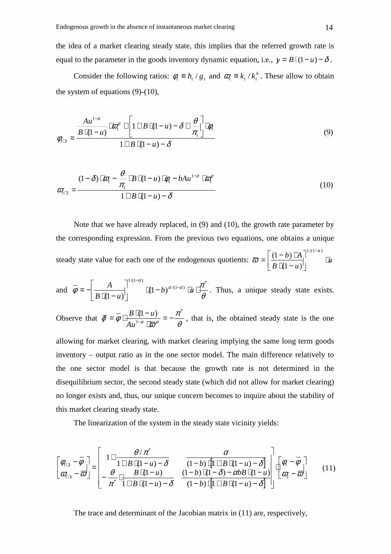
Consider the following ratios: ttt gh /≡φ and httt kk /≡ω . These allow to obtain

the system of equations (9)-(10),

δ

φπθδω

φ

αα

−−⋅+

⋅

+−−⋅++⋅

−⋅=

−

+ )1(1

)1(1)1(

1

1 uB

uBuB

Aut

tt

t (9)

δ

ωφπθωδ

ω

αα

−−⋅+

⋅−⋅−⋅⋅−⋅−=

−

+ )1(1

)1()1( 1

1 uB

bAuuB ttt

t

t (10)

Note that we have already replaced, in (9) and (10), the growth rate parameter by

the corresponding expression. From the previous two equations, one obtains a unique

steady state value for each one of the endogenous quotients: uuB

Ab ⋅

−⋅⋅−=

− )1/(1

)1(

)1(α

ω

and θπφ αα

α *)1/(

)1/(1

)1()1(

⋅⋅−⋅

−⋅−= −

−

ubuB

A. Thus, a unique steady state exists.

Observe that θπ

ωφϕ αα

*

1

)1( −=⋅−⋅⋅= −Au

uB, that is, the obtained steady state is the one

allowing for market clearing, with market clearing implying the same long term goods

inventory – output ratio as in the one sector model. The main difference relatively to

the one sector model is that because the growth rate is not determined in the

disequilibrium sector, the second steady state (which did not allow for market clearing)

no longer exists and, thus, our unique concern becomes to inquire about the stability of

this market clearing steady state.

The linearization of the system in the steady state vicinity yields:

[ ]

[ ]

−−

⋅

−−⋅+⋅−−⋅−−⋅−

−−⋅+−⋅⋅−

−−⋅+⋅−−−⋅++

=

−−

+

+

ωωφφ

δαδ

δπθ

δα

δπθ

ωωφφ

t

t

t

t

uBb

ubBb

uB

uBuBbuB

)1(1)1(

)1()1()1(

)1(1

)1()1(1)1()1(1

/1

*

*

1

1 (11)

The trace and determinant of the Jacobian matrix in (11) are, respectively,

Endogenous growth in the absence of instantaneous market clearing 15

[ ]δαπθδ

−−⋅+⋅−−⋅−+−⋅−+=

)1(1)1(

)1()/1()1(1)(

*

uBb

ubBbJTr ;

[ ] [ ]2* )1(1

)1(1

)1(1)1(

)1()1()1()(

δδα

πθ

δαδ

−−⋅+−−⋅+⋅+

−−⋅+⋅−−⋅−−⋅−=

uB

uB

uBb

ubBbJDet .

Trace and determinant expressions tell us that a positive ratio */πθ requires

)(1)( JDetJTr >− , i.e., feasible long term results imply that stability (two eigenvalues

inside the unit circle) will not exist, since the stability condition 0)()(1 >+− JDetJTr

is violated.

Replacing the */πθ ratio in the determinant expression by the corresponding

value in terms of the trace, one obtains )()1(1

)1(1)( JTr

uB

uBJDet ⋅

−−⋅+−−⋅++=δδαν , with ν a

combination of parameters b, B, u, α and δ. The previous expression indicates the

presence of a determinant – trace relation with a positive but lower than one slope.

Thus, the dynamics of the system is given by a relation that starts immediately after the

bifurcation point 1)()( −= JTrJDet and with a slope lower than the one of the

bifurcation line. This is depicted in figure 2. This figure reveals that the system is

saddle-path stable for a relatively low value of the ratio */πθ , undergoing then a

bifurcation that leads to instability.

*** Figure 2 ***

The saddle-path stability condition is:

[ ] [ ][ ]δα

δαπθ

−−⋅+⋅−−−⋅+⋅⋅−−⋅−⋅<<

)1(1)1(

)1(1)1(1)1(0

* uBb

uBbuB. If the upper bound of the

double inequality is crossed, then we no longer have 1)( <JDet and the stability

possibility vanishes.

The two-sector model, that involves the presence of two forms of capital and

where no control variable is considered, has a unique market clearing steady state

which, for relatively low values of */πθ , is saddle-path stable. Thus, convergence to

the steady state is not guaranteed independently of the initial point. The combination

between the initial quantities of physical and human capital must be such that it puts the

system on the stable trajectory allowing for convergence to the steady state; otherwise,

variables will depart from the long run equilibrium.

Endogenous growth in the absence of instantaneous market clearing 16 5. Getting Closer to the Classics: Non-Equilibrium

Intertemporal Optimization

In the previous sections, one has assumed that the representative agent does not

optimize consumption or the distribution of inputs across sectors in order to obtain the

best feasible intertemporal utility of consumption. However, non optimization is not a

pre-requisite of the non market clearing analysis. In this section, we develop a one

sector model similar to the one in sections 2 and 3 where, nevertheless, the constant

marginal propensity to consume is replaced by a process of intertemporal utility

maximization.

Let the representative consumer maximize

[ ]∑+∞

=

⋅=0

0 )(t

tt cuU β (12)

Parameter β∈(0,1) is the discount factor and u(ct) is the instantaneous utility

function. We consider a simple continuous and differentiable utility function with

diminishing marginal consumption utility of the logarithmic form, u(ct)=ln(ct). The

maximization of U0 is subject to resource constraints (1) and (2) and to the inflation

equations (4) and (6). The main distinctive feature relatively to the problem of section 2,

is that now consumption is not a fixed proportion of income, but the result of an

optimization process.

Besides consumption, it is assumed that the inflation rate is also a control variable

of the problem. The private economy is, after all, the first responsible by determining

price changes. However, recall that the proposed framework gives a determinant role to

the monetary authority in what concerns price setting: it is chosen an interest rate rule

that makes prices to converge to a specified target. Thus, the assumption of optimization

of the inflation rate, in order to maximize utility, by the representative agent is relevant

if the monetary authority sets its policy taking into account the best interest of the

private economy. In practical terms, the analytical treatment of the model will show that

the possibility of control of inflation will not impose any constraint on the action of the

central bank; it just sets a relation between shadow-prices capable of simplifying the

problem’s dynamics.

The Hamiltonian function of the problem is:

Endogenous growth in the absence of instantaneous market clearing 17

⋅

++⋅+

+

+⋅⋅⋅−=

+

+

tt

tht

tttt

ytt

ht

yttttt

hyp

ychApcuppchyH

πθγβ

δπθβπ

1

1)(),,,,,(

ht

yt pp , ∈IR are the co-state variables of yt and ht, respectively.

First-order optimality conditions are:

yttu pAcH 1/10 +=⇒= β ;

ht

yt pApH 110 ++ =⇒=π ;

ht

yt

yty

yt

yt pppHpp 111 )1( +++ −=−⋅−⇒−=− ββδβ ;

( ) yt

ht

hth

ht

ht pAppHpp 1

*1

*1 )/(/1 +++ ⋅⋅=−⋅++⇒−=− βπθβπθγβ ;

0lim =+∞→

yt

tt

tpy β (transversality condition);

0lim =+∞→

ht

tt

tph β (transversality condition).

From the first three optimality conditions, it is obtained a constant growth rate for

consumption:

1)1(1 −−+⋅=−+ δβ A

c

cc

t

tt (13)

Note that, as we have remarked, the second optimality condition does not impose

any constraint that the central bank must obey when acting over the inflation rate; it just

generates a relation between co-state variables such that consumption will grow in every

period at a same rate.

The dynamic analysis will proceed by recovering the goods inventory – output

ratio of section 2, ϕt, and by defining the consumption – output ratio ttt yc /≡ψ . Once

again, the steady state is defined as the state in which all real variables grow at a same

constant rate and, thus, ϕ and ψ are constant values. A pair of difference equations

describes the dynamics of the problem under study,

)/(1

/)1(11

ttt

tttt A ψπϕθδ

πϕθϕγϕ+⋅⋅−−

⋅+⋅++=+ (14)

Endogenous growth in the absence of instantaneous market clearing 18

tttt

t A

A ψψπϕθδ

δβψ ⋅+⋅⋅−−

−+⋅=+ )/(1

)1(1 (15)

The definition of steady state implies that the steady state growth rate must be the

one presented in equation (13). The definition of market clearing steady state requires,

as seen in section 3, that the long run growth rate is γ. Hence, for the case in

appreciation, since one wants to discuss the possibility of convergence to market

clearing, it is true that 1)1( −−+⋅= δβγ A . Replacing γ in system (14)-(15), we get a

unique solution θπϕ /*−= , )1(1 δβψ −+⋅−= A

A. This steady state point allows for

market clearing.

The stability of this equilibrium point is now addressed. In the vicinity of ),( ψϕ ,

the system takes the linearized form:

−−

⋅

⋅−−+⋅

−−+⋅

−+=

−−

+

+

ψψϕϕ

βπθ

ββ

δβθπ

δβπθ

ψψϕϕ

t

t

t

t A

A

A

A

11)1(

/

)1(

/1

*

**

1

1 (16)

The trace and the determinant of the Jacobian matrix in (16) are, respectively,

)1(

/1)(

*

δβπθ

ββ

−+⋅−++=

A

AJTr ;

)1(

/1)(

2

*

δββπθ

β −+⋅−+=A

AJDet .

Stability conditions come,

021

)1(

112)()(1

*>

−⋅+⋅−+⋅

++⋅=++ AA

JDetJTrπθ

ββ

δβββ

;

0)1(

11)()(1

*>⋅

−+⋅⋅−=+−

πθ

δβββ

AJDetJTr ;

0)1(

/1)(1

2

*

>−+⋅

−−−−=−δβ

βπθβ

βA

AJDet .

The second condition is satisfied for any positive π* (we continue to consider that

the inflation target is positive and, thus, the steady state goods inventory is a negative

amount). The other two conditions may hold or may not hold, depending on parameter

values. A diagram drawn in the trace-determinant referential will allow to understand

under which conditions stability prevails.

Endogenous growth in the absence of instantaneous market clearing 19

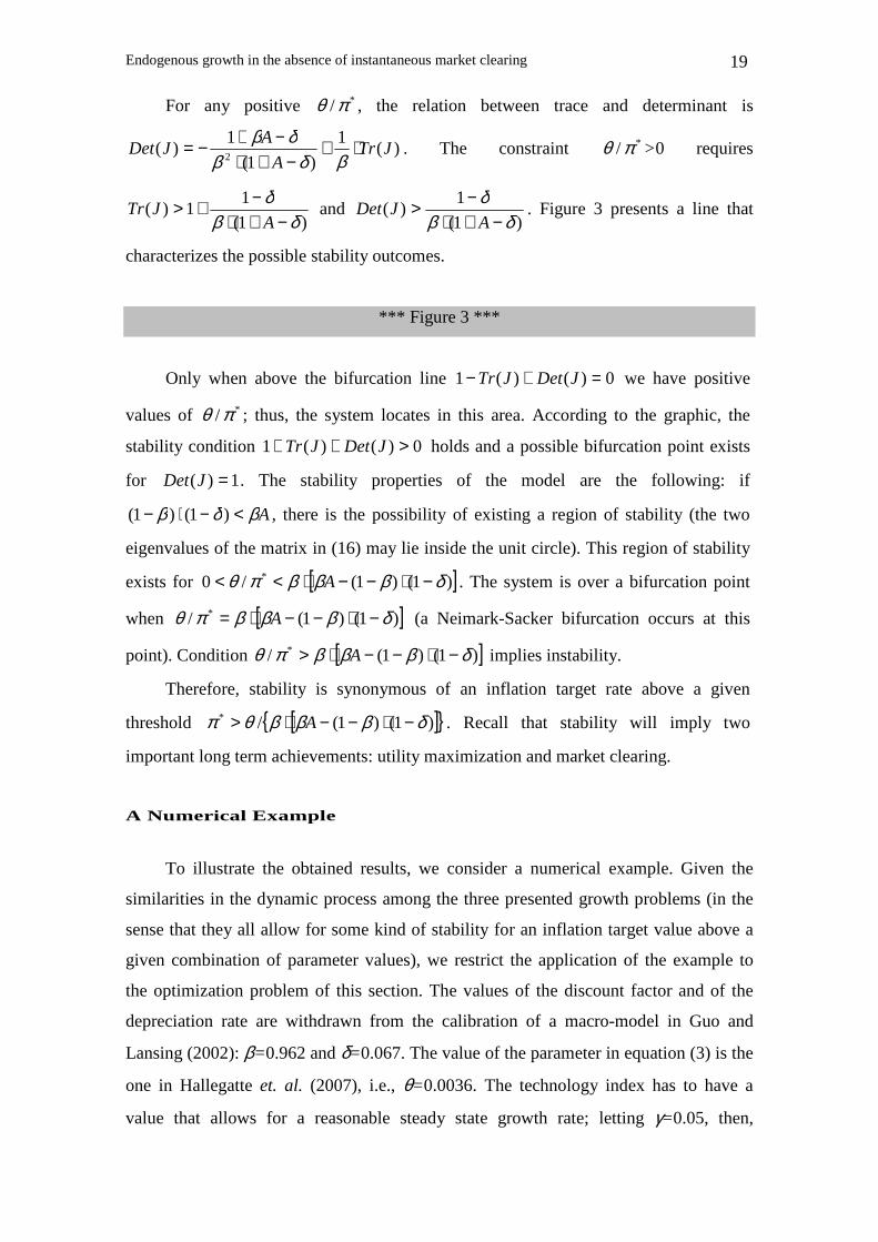
For any positive */πθ , the relation between trace and determinant is

)(1

)1(

1)(

2JTr

A

AJDet ⋅+

−+⋅−+−=

βδβδβ

. The constraint */πθ >0 requires

)1(

11)(

δβδ

−+⋅−+>

AJTr and

)1(

1)(

δβδ

−+⋅−>

AJDet . Figure 3 presents a line that

characterizes the possible stability outcomes.

*** Figure 3 ***

Only when above the bifurcation line 0)()(1 =+− JDetJTr we have positive

values of */πθ ; thus, the system locates in this area. According to the graphic, the

stability condition 0)()(1 >++ JDetJTr holds and a possible bifurcation point exists

for 1)( =JDet . The stability properties of the model are the following: if

Aβδβ <−⋅− )1()1( , there is the possibility of existing a region of stability (the two

eigenvalues of the matrix in (16) may lie inside the unit circle). This region of stability

exists for [ ])1()1(/0 * δβββπθ −⋅−−⋅<< A . The system is over a bifurcation point

when [ ])1()1(/ * δβββπθ −⋅−−⋅= A (a Neimark-Sacker bifurcation occurs at this

point). Condition [ ])1()1(/ * δβββπθ −⋅−−⋅> A implies instability.

Therefore, stability is synonymous of an inflation target rate above a given

threshold [ ]{ })1()1(/* δβββθπ −⋅−−⋅> A . Recall that stability will imply two

important long term achievements: utility maximization and market clearing.

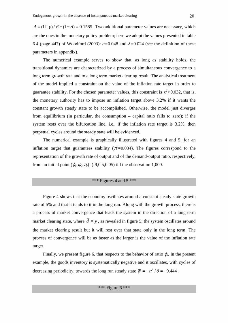
A Numerical Example

To illustrate the obtained results, we consider a numerical example. Given the

similarities in the dynamic process among the three presented growth problems (in the

sense that they all allow for some kind of stability for an inflation target value above a

given combination of parameter values), we restrict the application of the example to

the optimization problem of this section. The values of the discount factor and of the

depreciation rate are withdrawn from the calibration of a macro-model in Guo and

Lansing (2002): β=0.962 and δ=0.067. The value of the parameter in equation (3) is the

one in Hallegatte et. al. (2007), i.e., θ=0.0036. The technology index has to have a

value that allows for a reasonable steady state growth rate; letting γ=0.05, then,

Endogenous growth in the absence of instantaneous market clearing 20

1585.0)1(/)1( =−−+= δβγA . Two additional parameter values are necessary, which

are the ones in the monetary policy problem; here we adopt the values presented in table

6.4 (page 447) of Woodford (2003): a=0.048 and λ=0.024 (see the definition of these

parameters in appendix).

The numerical example serves to show that, as long as stability holds, the

transitional dynamics are characterized by a process of simultaneous convergence to a

long term growth rate and to a long term market clearing result. The analytical treatment

of the model implied a constraint on the value of the inflation rate target in order to

guarantee stability. For the chosen parameter values, this constraint is π*>0.032, that is,

the monetary authority has to impose an inflation target above 3.2% if it wants the

constant growth steady state to be accomplished. Otherwise, the model just diverges

from equilibrium (in particular, the consumption – capital ratio falls to zero); if the

system rests over the bifurcation line, i.e., if the inflation rate target is 3.2%, then

perpetual cycles around the steady state will be evidenced.

The numerical example is graphically illustrated with figures 4 and 5, for an

inflation target that guarantees stability (π*=0.034). The figures correspond to the

representation of the growth rate of output and of the demand-output ratio, respectively,

from an initial point (ϕ0,ψ0,π0)=(-9,0.5,0.05) till the observation 1,000.

*** Figures 4 and 5 ***

Figure 4 shows that the economy oscillates around a constant steady state growth

rate of 5% and that it tends to it in the long run. Along with the growth process, there is

a process of market convergence that leads the system in the direction of a long term

market clearing state, where yd = , as revealed in figure 5; the system oscillates around

the market clearing result but it will rest over that state only in the long term. The

process of convergence will be as faster as the larger is the value of the inflation rate

target.

Finally, we present figure 6, that respects to the behavior of ratio ϕt. In the present

example, the goods inventory is systematically negative and it oscillates, with cycles of

decreasing periodicity, towards the long run steady state 444.9/* −=−= θπϕ .

*** Figure 6 ***

Endogenous growth in the absence of instantaneous market clearing 21 6. Policy Implications and Discussion

Mainstream growth theory, including endogenous growth models, has always

involved a time paradox; while the process of resource accumulation and generation of

wealth is subject to an evolution from an initial state to a steady state, no similar process

is found in what concerns market adjustment. Market equilibrium is instantaneous and

no place is left for a dynamic transition from an initial state of excess demand or excess

supply to a market clearing outcome.

The possibility of market adjustment is easily introduced by considered a goods

inventory that is filled with increased output and emptied with increased demand.

Establishing, then, a relation between the goods inventory and the growth of the price

level, the framework of simultaneous growth and market disequilibrium becomes ready

to the dynamic analysis. The behavior of the inflation rate can be understood, following

the observed reality in modern economies, as the strict result of a monetary policy that

uses the nominal interest rate as an instrument to directly determine the evolution of the

price level.

The non equilibrium endogenous growth model was analyzed under three different

settings. First, a simple consumption function, in which consumption is a constant share

of the income level, was considered. This allowed addressing dynamics under a one-

dimensional difference equation. Assuming that the representative agent aims at a

market clearing steady state, one observes that there are two steady state points; one of

them guarantees long term market clearing alongside with endogenous growth at a

given rate, while the other leads to situations of excess demand or excess supply.

The study of stability indicates that the two points represent different stability

outcomes (when one is stable, the other is unstable); in particular, the market clearing

steady state prevails when the inflation rate target set by the central bank is bounded in a

given interval; the boundaries of this interval are dependent on the technology index of

the production function, on the depreciation rate of capital, on the marginal propensity

to consume and on the elasticity between inflation and the goods inventory per unit of

demand. In this way, we understand the relevant role of monetary policy over growth,

which is absent in conventional growth models; the central bank may change the

inflation target in order to guarantee a situation of long term market equilibrium (a

situation where long term growth is compatible with a coincidence of interests between

demand and supply agents).

Endogenous growth in the absence of instantaneous market clearing 22

On a second stage, an education sector was introduced. This has changed

significantly the dynamics of the system because while the disequilibrium continues

associated with the final goods sector, the source of endogenous growth is now linked to

the linear shape of the human capital production function. A unique steady state exists

when the representative agent searches for a market clearing equilibrium. The stability

of this steady state point requires two important types of policy measures. First, the

monetary authority should set the inflation rate target above a combination of

parameters that involve the inflation – inventory sensitivity parameter, the capital

depreciation rate, the marginal propensity to consume, the output – physical capital

elasticity, the share of human capital allocated to the production of physical goods and

the education sector technology (but not the goods sector technology). This relatively

high value of the inflation target guarantees the existence of a saddle-path steady state.

The second policy measure has to do with the need of putting the system in the

stable trajectory in order to converge to the long run equilibrium. Because the system

does not involve any control variable, the private economy cannot produce this

coincidence between an initial state and the convergence path. It has to be artificially

generated by means of, for instance, a fiscal policy that drives the incentives for the

accumulation of inputs. Basically, policy should be aimed at the formation of a relation

between the amount of physical capital and human capital that puts the system over the

saddle path.

Finally, a third model has abandoned the simple linear consumption function,

replacing it by an optimization behavior of the private economy representative agent.

This controls, as a household, the level of consumption and, as a firm, the way prices

evolve over time. With these two control variables, the agent maximizes consumption

utility. Once again, we have looked at the eventual existence of a market clearing steady

state. It exists and it is unique. The analysis of local dynamics allows to find two

possible stability outcomes: instability, for relatively low values of the inflation rate

target (below a combination of parameters involving the technology of production, the

parameter of the inflation – goods inventory per unit of demand equation, the

depreciation of capital and the rate of discount of future utility), and stability (that exists

regardless of the initial state) for relatively high values of the inflation rate target. Here,

as in the other models, a low inflation rate target is advantageous because it allows for a

not too negative steady state level of the goods inventory (i.e., the delivery lag is

straightened if price increases are kept low); nevertheless, it can lead to an unstable

Endogenous growth in the absence of instantaneous market clearing 23 outcome and therefore a divergence from the market clearing endogenous growth steady

state.

The conclusion is that if one departs from the strong assumption of instantaneous

market clearing when analyzing growth processes, monetary policy becomes relevant

since price changes are an important influence over the real economy. Monetary policy

should be such that the selected interest rate rule allows for a convergence to an

inflation target. In turn, the inflation target must be low (to avoid cases of too high

instantaneous underproduction) but not so low that it prevents convergence to the

desired long run state.

A final point of interest concerns the comparison of the proposed setup with the

basic AK growth model with instantaneous market clearing; this has plain and

straightforward transitional dynamics, i.e., output grows in every time moment at

exactly the same rate and the study of stability becomes irrelevant. In this sense, the

assumption of a market adjustment process alongside with the growth process

introduces the possibility of appealing dynamics otherwise absent and in which, as seen

in the figures of the numerical example of section 5, periods of excess demand alternate

with periods of excess supply, producing sequential phases of low growth and high

growth (relatively to the long run rate).

Appendix – Derivation of the Optimal and Stable

Interest Rate Rule

The goal of this appendix is to derive the inflation equation of motion (6) from a

standard new Keynesian monetary policy model, presented as a fully deterministic

problem in discrete time.

Consider that the monetary authority maximizes the value of function V0,

[ ]

−+−⋅⋅⋅−= ∑

+∞

=0

2*2*00 )()(

2

1

ttt

t xxaEV ππβ (a1)

Variables tπ ,xt∈IR represent the inflation rate and the output gap; this last variable

is defined as the difference, in logs, between effective and potential output. Parameters

π* and x* are the target values for each one of the variables; these values are selected by

the central bank according to its policy goals. The constant a≥0 represents the weight

Endogenous growth in the absence of instantaneous market clearing 24 attributed to the real stabilization of the economy in the objective function, and β∈(0,1)

is the discount factor.

The two constraints of the problem are the usual IS dynamic equation (a2) and a

new Keynesian Phillips curve, (a3),

11)( ++ +−⋅−= tttttt xEErx πζ , x0 given. (a2)

1+⋅+= tttt Ex πβλπ , π0 given. (a3)

Terms Etπt+1 and Etxt+1 correspond to the private agents’ expectations concerning

next period inflation and output gap. Parameters ζ>0 and λ∈(0,1) are, respectively, the

output gap – interest rate elasticity and a measure of price stickiness (the closer λ is

from 0, the higher is the degree of price stickiness). Variable rt∈IR , the nominal interest

rate, is the control variable of the problem – the central bank will choose rt in order to

attain an optimal result, given the intertemporal objective function V0.

Considering perfect foresight (Etπt+1=πt+1 and Etxt+1=xt+1), as one implicitly does

in the analysis of the real economy across the text, and defining pt and qt as the co-state

variables associated to xt and tπ , respectively, one writes the Hamiltonian function of

the problem,

[ ]

⋅−⋅−⋅+

⋅+⋅−⋅−⋅+

−+−⋅⋅−=

+

+

ttt

tttt

ttttttt

xq

xrp

xxaqprxH

βλπ

βββ

βλπ

βζβ

πππ

1

1

)()(2

1),,,,(

1

1

2*2*

The first-order conditions are,

00 =⇒= tr pH ;

)( *11 xx

aqHpp ttxtt −⋅−=⇒−=−⋅ ++ λ

β ;

*11 ππβ π −=−⇒−=−⋅ ++ ttttt qqHqq ;

0lim =⋅⋅+∞→ t

tt

tpx β (transversality condition);

0lim =⋅⋅+∞→ t

tt

tqβπ (transversality condition).

From the optimality conditions, one computes the following difference equation,

Endogenous growth in the absence of instantaneous market clearing 25

*2

1 1 πλπβλ

βλ ⋅+⋅−⋅

+=+ aa

xa

x ttt (a4)

Equation (a4) and the Phillips curve constitute a two-equation – two-endogenous

variables linear system, which is presentable as,

−−

⋅

−

−+=

−−

+

+

ππββ

λβλ

βλ

ππ t

t

t

t xxaaxx

1

12

1

1 (a5)

By imposing tt xxx =≡ +1 and tt πππ =≡ +1 , one obtains the steady state pair

⋅−= ** ;1

);( ππλ

βπx . The eigenvalues of the Jacobian matrix in (a5) are 0<ε1<1

and ε2>1,

ββλβ

βλβεε 1

2

)1(

2

)1(,

222

21 −

++⋅++⋅=a

a

a

am (a6)

Because one of the eigenvalues locates inside the unit circle and the other does

not, the system is characterized by a saddle-path stable equilibrium: there is one stable

dimension in the two-dimensional space that defines the system. Therefore, we can

compute the saddle-path, i.e., the stable trajectory. This is )(1

2 xxp

ptt −⋅=− ππ , with

p1 and p2 the elements of an eigenvector associated to the eigenvalue inside the unit

circle. One finds the expression ttx πλβεπ

λεβ ⋅−−⋅−⋅= 1*1 1)1(

. Replacing the output

gap expression just found into the Phillips curve, we obtain the inflation equation in (6).

We have obtained equation (6) in two steps:

i) First, the central bank builds an objective function and it adopts an optimizing

behavior;

ii) Optimization leads to an infinite number of trajectories in the two dimensional

space of the system, but only one of these trajectories is stable. Thus, the central bank

Endogenous growth in the absence of instantaneous market clearing 26 also chooses to put the economy in the stable path, which guarantees the convergence to

the inflation steady state value (that coincides with the target defined by the central

bank).

The two previous goals are attained through the manipulation of the monetary

policy instrument: the nominal interest rate. Note that from the IS equation (a2), the

interest rate corresponds to the expression

11 )(1

++ +−⋅= tttt xxr πζ

(a7)

Hence, imposing the interest rate rule in (a8), one obtains the inflation dynamic

equation that simultaneously translates a situation of intertemporal optimization and

selection of an inflation stable path,

*111 )1()(

1 πεπεζ

⋅−+⋅+−⋅= + tttt xxr (a8)

Optimality and stability require the central bank to increase the nominal interest

rate whenever there is an expected positive change in the output gap and whenever

contemporaneous inflation rises (the opposite changes imply an interest rate decrease).

Observe that under rule (a8), the steady state real interest rate is zero: ** π=r .

References

Asada, T.; C. Chiarella and P. Flaschel (2003). “Keynes-Metzler-Goodwin Model

Building: The Closed Economy.” UTS School of Finance and Economics Working

Paper No. 124.

Barro R. J. and H. I. Grossman (1971). “A General Disequilibrium Model of Income

and Employment.” American Economic Review, vol. 61, pp. 82-93.

Bénassy, J. P. (1975). “Neo-Keynesian Disequilibrium in a Monetary Economy.”

Review of Economic Studies, vol. 42, pp. 503-523.

Bénassy, J. P. (1993). “Nonclearing Markets: Microeconomic Concepts and

Macroeconomic Applications.” Journal of Economic Literature, vol. 31, pp. 732-

761.

Endogenous growth in the absence of instantaneous market clearing 27 Bénassy, J. P. (2002). The Macroeconomics of Imperfect Competition and Nonclearing

Markets. Cambridge, MA: MIT Press.

Blackburn, K. (1999). “Can Stabilization Policy Reduce Long-run Growth?” Economic

Journal, vol. 109, pp. 67–77.

Bond, E.; P. Wang and C. Yip (1996). “A General Two-Sector Model of Endogenous

Growth with Human and Physical Capital: Balanced Growth and Transitional

Dynamics.” Journal of Economic Theory, vol. 68, pp. 149-173.

Caballé, J. and M. S. Santos (1993). “On Endogenous Growth with Physical and Human

Capital.” Journal of Political Economy, vol. 101, pp. 1042-1067.

Cellarier, L. (2006). “Constant Gain Learning and Business Cycles.” Journal of

Macroeconomics, vol. 28, pp. 51-85.

Chiarella, C. and P. Flaschel (2000). The Dynamics of Keynesian Monetary Growth:

Macro Foundations. Cambridge, UK: Cambridge University Press.

Chiarella, C.; P. Flaschel and R. Franke (2005). Foundations for a Disequilibrium

Theory of the Business Cycle. Cambridge, UK: Cambridge University Press.

Clarida, R.; J. Gali and M. Gertler (1999). “The Science of Monetary Policy: A New

Keynesian Perspective.” Journal of Economic Literature, vol. 37, pp. 1661-1707.

Clower R. (1965). “The Keynesian Counter-Revolution: a Theoretical Appraisal.” In: F.

H. Hahn and F. P. R. Brechling (eds.), The Theory of Interest Rates (Proceedings

of a Conference held by the International Economic Association). London:

MacMillan.

Dutt, A. K. (2006). “Aggregate Demand, Aggregate Supply and Economic Growth.”

International Review of Applied Economics, vol. 20, pp. 319-336.

Flaschel, P.; R. Franke and W. Semmler (1997). Dynamic Macroeconomics: Instability,

Fluctuations and Growth in Monetary Economies. Cambridge, MA: the MIT

Press.

Geanakoplos, J. D. and H. M. Polemarchakis (1986). “Walrasian Indeterminacy and

Keynesian Macroeconomics.” Review of Economic Studies, vol. 53, pp. 755-793.

Gómez, M. A. (2003). “Optimal Fiscal Policy in the Uzawa-Lucas Model with

Externalities.” Economic Theory, vol. 22, pp. 917-925.

Gómez, M. A. (2004). “Optimality of the Competitive Equilibrium in the Uzawa-Lucas

Model with Sector-specific Externalities.” Economic Theory, vol. 23, pp. 941-948.

Goodfriend, M. and R. G. King (1997). "The New Neoclassical Synthesis and the Role

of Monetary Policy." in B. Bernanke and J. Rotemberg (eds.), NBER

Macroeconomics Annual 1997, Cambridge, Mass.: MIT Press, pp. 231-282.

Endogenous growth in the absence of instantaneous market clearing 28 Guo, J. T. and K. J. Lansing (2002). “Fiscal Policy, Increasing Returns and Endogenous

Fluctuations.” Macroeconomic Dynamics, vol. 6, pp. 633-664.

Hallegatte, S. and M. Ghil (2007). “Endogenous Business Cycles and the Economic

Response to Exogenous Shocks.” Fondazione Enrico Mattei, nota di lavoro

20.2007.

Hallegatte, S.; M. Ghil; P. Dumas and J. C. Hourcade (2007). “Business Cycles,

Bifurcations and Chaos in a Neo-Classical Model with Investment Dynamics.”

Journal of Economic Behavior and Organization, forthcoming.

Ladrón-de-Guevara, A.; S. Ortigueira and M. S. Santos (1997). “Equilibrium Dynamics

in Two-sector Models of Endogenous Growth.” Journal of Economic Dynamics

and Control, vol. 21, pp. 115-143.

Leijonhufvud, A. (1968). On Keynesian Economics and the Economics of Keynes: a

Study in Monetary Theory, New York and London: Oxford University Press.

Lucas, R. E. (1988). “On the Mechanics of Economic Development.” Journal of

Monetary Economics, vol. 22, pp. 3-42.

Mankiw, N. G. (2006). “The Macroeconomist as Scientist and Engineer.” Journal of

Economic Perspectives, vol. 20, pp. 29-46.

Malinvaud E. (1977). The Theory of Unemployment Reconsidered. Oxford: Basil

Blackwell.

Mulligan, C. B. and X. Sala-i-Martin (1993). “Transitional Dynamics in Two-Sector

Models of Endogenous Growth.” Quarterly Journal of Economics, vol. 108, pp.

739-773.

Palley, T. I. (1996). “Growth Theory in a Keynesian Model: Some Keynesian

Foundations for New Growth Theory.” Journal of Post Keynesian Economics, vol.

19, pp. 113–135.

Palley, T. I. (2003). “Pitfalls in the Theory of Growth: an Application to the Balance of

Payments Constrained Growth Model.” Review of Political Economy, vol. 15, pp.

75–84.

Patinkin, D. (1965). Money, Interest and Prices, 2nd edition, New York: Harper and

Row.

Raberto, M.; A. Teglio and S. Cincotti (2006). “A Dynamic General Disequilibrium

Model of a Sequential Monetary Production Economy.” Chaos, Solitons and

Fractals, vol. 29, pp. 566-577.

Rebelo, Sérgio (1991). “Long-Run Policy Analysis and Long-Run Growth.” Journal of

Political Economy, vol. 99, nº 3, pp. 500-521.

Endogenous growth in the absence of instantaneous market clearing 29 Woodford, M. (2003). Interest and Prices: Foundations of a Theory of Monetary

Policy. Princeton, New Jersey: Princeton University Press.

Tables and Figures

Cases Stable

steady state Market clearing

12

)1(2

−

−⋅>

bA

δ

)1(2)12(

*

δθ

πθ

−⋅−⋅−<<

AbA

1ϕ Yes

12

)1(2

−

−⋅>

bA

δ

A

θπ << *0 ∨

)1(2)12(

*

δθ

π−⋅−⋅−

>Ab

2ϕ

No

−⋅−⋅−><

<>

)1(2)12(

* if

* if

δθ

π

θπ

Abyd

Ayd

12

)1(2

−

−⋅<

bA

δ

A

θπ >*

1ϕ Yes

12

)1(2

−

−⋅<

bA

δ

A

θπ << *0

2ϕ No

yd >

Table 1 – Steady state stability.

Endogenous growth in the absence of instantaneous market clearing 2

Figure 1 – Stability results in the constant propensity to consume one-sector model.

Figure 2 – Trace-determinant diagram in the two-sector model.

1-Det(J)=0

Tr(J)

Det(J) 1+Tr(J)+Det(J)=0 1-Tr(J)+Det(J)=0

-π*/θ

-1/A

-1/A

-π*/θ ϕt+1

ϕt

stable

unstable

π*<θ/A

-1/A

-1/A

-π*/θ

-π*/θ

ϕt+1

ϕt

stable

unstable

π*>θ/A

Endogenous growth in the absence of instantaneous market clearing 3

Figure 3 – Trace-determinant diagram in the optimization problem.

gr y

-0,1

-0,05

0

0,05

0,1

0,15

1 61 121 181 241 301 361 421 481 541 601 661 721 781 841 901 961

Figure 4 – Numerical example: output growth rate dynamics.

)1(

1

δβδ

−+⋅−

A

1-Det(J)=0

Tr(J)

Det(J) 1+Tr(J)+Det(J)=0 1-Tr(J)+Det(J)=0

)1(

11

δβδ

−+⋅−+

A

Endogenous growth in the absence of instantaneous market clearing 4

d/y

0

0,5

1

1,5

2

2,5

1 60 119 178 237 296 355 414 473 532 591 650 709 768 827 886 945

Figure 5 – Numerical example: demand-output ratio dynamics.

fi

-25

-20

-15

-10

-5

0

1 59 117 175 233 291 349 407 465 523 581 639 697 755 813 871 929 987

Figure 6 – Numerical example: goods inventory-output ratio dynamics.