Endogenous Debt Constraints in a Life-Cycle Modelwith an Application to Social Security∗

David AndolfattoSimon Fraser University

Rimini Centre for Economic Analysisdandolfa@sfu.ca

Martin GervaisUniversity of Southampton

gervais@soton.ac.uk

December 17, 2007

Abstract

This paper develops a simple life-cycle model that embeds a theory of debtrestrictions based on the existence of inalienable property rights a la Kehoeand Levine (1993, 2001). In our environment, net debtors have the option ofdefaulting on unsecured debt at the cost of being subjected to wage garnish-ment and/or having some or all of their future assets seized by creditors. Oneadvantage of our framework is that it encompasses two standard versions of thelife-cycle model: one with perfect capital markets and one with a non-negativenet worth restriction. We study the impact of a payroll financed social securitysystem to illustrate the role of endogenous debt constraints and compare our re-sults to a model with exogenous debt constraints. Whereas the aggregate effectsare similar under both types of constraints, the distributional consequences arefound to be significantly different across debt regimes.

Journal of Economic Literature Classification Numbers: E21; E62; H55keywords: Life-cycle; Debt Constraints; Social Security

∗We would like to thank seminar participants at the NBER Summer Institute, The SED confer-ence in Costa Rica, The University of Western Ontario and the Richmond Fed for helpful commentsand suggestions. Both authors gratefully acknowledge financial support from the Social Sciencesand Humanities Research Council of Canada.

1 Introduction

This paper develops a simple life-cycle model that embeds a theory of debt restrictions

based on the existence of inalienable property rights (Kehoe and Levine (1993, 2001)).

In our environment, net debtors (typically young individuals with bright futures)

have the option of defaulting on unsecured debt at the cost of being subjected to

wage garnishment and/or having some or all of their future assets seized by creditors.

One advantage of our framework is that it encompasses two standard versions of the

life-cycle model: one with perfect capital markets and one with a non-negative net

worth restriction.

Our environment differs in two important ways from typical models with ‘en-

dogenous debt constraints’, such as Kehoe and Levine (1993, 2001), Kocherlakota

(1996), Alvarez and Jermann (2000), and Krueger and Perri (2005). First, the in-

come fluctuations which give rise to our debt constraint emanate purely from life-cycle

considerations. Since these papers use the infinitely-lived agent abstraction, individ-

uals need to face other kinds of fluctuations in order for the default option to be

meaningful. In our framework, debt constraints arise from the simple fact that young

individuals with bright futures want to smooth their life-cycle consumption. But do-

ing so potentially entails contracting large amounts of unsecured loans. Once in their

peak earning years, these individuals may find defaulting on their loans an attractive

option. Since rational creditors take these incentives into account in their supply of

loans, individuals may find themselves debt constrained early in their life-cycle.

Second, whereas debt constraints in our environment arise from a default option,

the default option does not correspond to autarky.1 The default option in our frame-

work is meant to capture in a crude way the main aspects of the bankruptcy law.2

In essence, bankruptcy laws restrict the extent to which creditors can garnishee wage

income and seize an individual’s assets (current and future). Upon default—which

does not occur in equilibrium in the model—the rights to a fraction of an individ-

ual’s current and future assets and/or wage income that can be legally garnisheed

1In the typical framework, the penalty of defaulting is to be banned from future participation inthe financial market forever. This type of setup implies not only that individual defaulters can nolonger borrow, but also that they cannot lend.

2See Livshits et al. (2007) and Chatterjee et al. (2007) for detailed analyses of consumerbankruptcy.

2

are transferred to the creditors. The permanent nature of the punishment implies

that creditors will refrain from lending to individuals with a history of default. A by-

product of our theory, then, is that individuals face a non-negative net worth restric-

tion conditional on default—a familiar problem—rather than a lending constraint,

which obtains when autarky is assumed following loan default. In our framework,

the garnishment limits naturally translate into debt limits at the individual level: the

more creditors can garnishee, the more credit is extended to individuals. In other

words, harsher punishment upon default imply higher levels of debt, consistent with

the work of Mateos-Planas and Seccia (2006).

Following the work of Bulow and Rogoff (1989) on sovereign debt, it is well known

that the possibility of savings upon default in standard models implies that no credit

will ever be extended. In other words, ‘merely denying credit is not a sufficient threat

to create a loan market’ as Kehoe and Levine (2001) put it. The reason is simple:

since no individual would ever pay back a loan during their last period of life, no

credit will be extended to such an individual. But since it is known that default

would occur in the last period of life, there is no point in extending credit the period

before since individuals would default there as well, and so on. The reason why this

does not occur in our economy is because of the long lasting effect of default: when

an individual defaults, there is always some resources that creditors can garnishee in

future periods. This feature is what makes credit markets operational from the first

periods of individuals’ life.

Our framework offers a simple way of modeling debt constraints which respond

endogenously to exogenous changes in the environment. As an application of our

setup, we illustrate the role of endogenous debt constraints by studying the impact

of introducing a payroll-tax financed social security system. We compare our results

to those of the Hubbard and Judd (1987), who were among the first to examine the

welfare implications of a social security system in the context of a life-cycle model

with exogenous debt constraints. Because the U.S. social security systems is financed

primarily through a payroll tax, the burden of finance falls disproportionately on the

young and middle-aged members of the population who are approaching, or are in,

their peak earning years. The provision of social security is likely to reduce the de-

sired private saving (increase desired borrowing) among individuals in these younger

cohorts. But to the extent that individuals in this subgroup are debt-constrained, a

3

proportional payroll tax reduces consumption expenditures dollar for dollar, and as a

consequence, increases the welfare cost (reduces the benefit) of the government pro-

gram. Hubbard and Judd (1987) demonstrate that these effects can be quantitatively

important.

Through a parameterized version of our model, we show that the introduction of

a redistributive fiscal policy such as a pay-as-you-go social security system does affect

the functioning of private credit markets by tightening individuals’ debt constraints

(as the supply of private loans contracts). Thus, in contrast to exogenous non-negative

net-worth constraints, the consumption of debt constrained individuals may respond

more than one for one in the face of a payroll tax. Our findings indicate that whereas

the aggregate effect of introducing a social security system are similar whether the

debt constraint is endogenous or exogenous, its distributional effects are significantly

different. Rojas and Urrutia (2007) extend our analysis and show that our aggregate

results are robust to the introduction of idiosyncratic uncertainty. Furthermore, they

show that the transition following the elimination of social security is monotonic and

that while individuals alive at the time of the announcement suffer significant losses,

these losses are invariant to whether the debt constraint is endogenous or exogenous.

The rest of the paper is organized as follows. The next section lays down the

economic environment and studies the consumer’s problem under endogenous debt

constraints. In Section 3 we parameterize the model and investigate its behavior

under different parameters governing the bankruptcy code. The impact of a payroll

financed social security system under endogenous and exogenous debt constraints is

the subject of Section 4. Finally, concluding remarks are offered in section 5.

2 The Economic Environment

2.1 Consumers

Consider an economy populated by overlapping generations of individuals who live for

J periods, indexed by j = 1, 2, . . . , J . The population is assumed to grow at a constant

rate n per period, and we denote the share of age-j individuals in the population by

µj, which is time-invariant and satisfies µj = (1 + n)−1µj−1 for j = 2, 3, . . . , J and

4

∑Jj=1 µj = 1.

Individuals have preferences defined over deterministic sequences of consump-

tion cj; these preferences are represented by a utility function U(c1, c2, . . . , cJ) of

the following form:

U =J∑

j=1

βj−1u(cj), (1)

where u(·), the per-period felicity function, has the usual properties, and β > 0

represents the subjective discount factor.

Individuals are endowed with one unit of time in each period of their life, which

they supply inelastically. Individuals are able to transform one unit of time into ej

efficiency units of labor. The ability level of individuals within age cohort j varies

according to the density function fj(x). Note that these human capital endowments

evolve deterministically and are assumed to be observable by all parties.3 Although we

do not wish to diminish the role of idiosyncratic uncertainty, the idea we model here

is that the most important component of life-cycle variation in earnings-capabilities

is largely forecastable.

Individuals are born with zero assets and will leave the economy with zero assets;

there are no bequests. Let w denote the (after-tax) price of one raw unit of labor and

let R denote the gross real rate of interest. As well let aj denote the net beginning-of-

period asset position of an age-j individual. Individuals face the following sequence

of budget constraints:

cj + aj+1 ≤ wej + Raj + Tj, j = 1, 2, . . . , J ; (2)

where a0 = 0 and Tj represents a lump-sum government transfer which we later inter-

pret as a social security payment, that is, Tj will be zero for working-age individuals

and positive for retired individuals.

In the absence of any debt restrictions, the problem faced by individuals is to

maximize life-time utility (1) subject to the sequence of budget constraints (2). When

aj < 0, however, an age-j individual may find it optimal to default on his debt

obligations. An individual will choose to default if the utility associated with that

3See Andolfatto and Gervais (2006) for a life-cycle model with human capital accumulation andendogenous debt constraints.

5

alternative is higher than that of honoring his debt, if

Vs(as) ≡J∑

j=s

βj−su(cj) ≥ V ds , s = 2, . . . , J, (3)

where Vs and V ds denote the continuation payoff accruing to an age-s individual under

alternative strategies of not defaulting and defaulting, respectively. We will refer to

this inequality as the individual rationality constraint.

Default Option The consequences of defaulting on a loan depend on the structure

of the legal system, which limits the set of actions that creditors can take against

defaulters. In the context of this model, creditors can take two actions against de-

faulters: garnishee their wages (current and future) and seize their assets (future).

Accordingly, let 0 ≤ πw ≤ 1 denote the fraction of wage income that a creditor is

feasibly (or legally) able to garnishee and 0 ≤ πa ≤ 1 denote the fraction of physical

and/or financial assets that a creditor can feasibly seize (exclusive of the value of the

social security entitlement).

We now turn to the analysis of the model. We show that given the legal struc-

ture, computing the value of the default option involves solving a familiar consumer

problem with a non-negative net-worth restriction. We also show that, as one would

expect, the individual rationality constraint (3) implies an age-dependent borrowing

restriction.

Consumer Problem at age J The problem that an individual faces at age J

depends on whether default occurred in the past. Consider first the problem faced by

an individual who has never defaulted in the past and enters the last period of life with

assets aJ . If the asset position is positive, consuming all his income is his only option.

If aJ < 0, the individual has to choose between (i) consuming his income minus the

loan repayment (weJ + RaJ + TJ) or (ii) defaulting on his loan and consuming the

fraction of his income that cannot be garnisheed by creditors ((1 − πw)weJ + TJ).

There is thus a value of aJ under which both options are equally attractive, that is,

there exists aJ such that the individual rationality constraint (3) holds with equality:

VJ(aJ) = V dJ when

aJ = −πwweJ

R. (4)

6

Defaulting is optimal when assets are sufficiently low (aJ < aJ) for the loan repayment

(principal plus interest) to be larger than the amount of resources that creditors

can legally garnishee. Since this is known by creditors, the individual rationality

constraint at age-J effectively limits the set of asset positions that can be chosen at

age J − 1; this constraint is given by aJ ≥ aJ .

Next consider the problem faced by an age-J individual with a history of default.

First note that when default occurred, the property rights to the defaulter’s earnings

that can legally be garnisheed were transferred to creditors. Since the remainder of

the defaulter’s earnings is inalienable, an individual who has defaulted in the past

will default again on any loan that is extended to him. Anticipating this strategy,

no credit will ever be extended to an age-J individual who has defaulted in the past.

Note that the exact timing of the default is irrelevant for this borrowing constraint:

if an individual defaulted at some point in the past, today’s earnings are being gar-

nisheed. To summarize, the individual rationality constraint (3) implies the following

borrowing constraint:

aJ ≥−πwweJ

Rno default history,

0 default history.(5)

Generalization to Earlier Periods To make their decisions, younger individuals

need to consider the impact of defaulting on future earnings and future capital market

participation in addition to the direct impact on today’s consumption. As before, we

need to separate the problem according to default histories.

Consider first the problem faced by an age-s individual with a history of default,

entering the period with assets as. This problem is simplified by the fact that as ≥ 0,

so that no default decision needs to be made. To see this, note that defaulting is

optimal for any as < 0, for the property rights to all the defaulter’s earnings that can

legally be garnisheed were transferred to previous creditors. It follows that no creditor

will extend any credit to an individual with a history of default. An individual with

a history of default thus faces a non-negative net worth restriction for the rest of his

life. As a result, we need not concern ourselves with the possibility that an individual

may have defaulted many times in the past nor with the possibility that an individual

may default again in the future.

7

The above argument is very helpful in analyzing the default decision of an age-

s individual who has never defaulted in the past. We have just established that

in addition to having a fraction of earnings garnisheed, defaulting today eliminates

an individual’s ability to borrow in the future. Hence, the continuation value of

defaulting at age s (V ds ) is the solution to the following problem:

V ds ≡ max

J∑j=s

βj−su(cj) (6)

subject to

cs + as+1 ≤(1− πw)wes + Ts (7)

cj + aj+1 ≤(1− πw)wej + (1− πa)Raj + Tj, j = s + 1, . . . , J (8)

aj+1 ≥0, j = s, . . . , J − 1. (9)

Note that V ds does not vary with as, but that Vs(as) is strictly increasing in as.

4

There must therefore exist an asset position as such that Vs(as) = V ds . This asset

position is the smallest amount of asset (largest amount of debt) that can be chosen

at age s− 1. To summarize, the individual rationality constraint (3) at age s implies

the following borrowing constraint at age-s− 1:

as ≥

as no default in history,

0 default in history.(10)

The above analysis emphasizes that the individual rationality constraint faced by

an age-(j + 1) individual translates into a restriction on the set of asset positions

that can be chosen at age j. Naturally, this borrowing constraint, or the maximum

amount of debt that can be extended to an individual, depends on the same factors

that affect the incentive to default (age, current asset position, and legal structure).

4This result only requires the utility function to be increasing in consumption. In general, in-creasing as increases consumption in all remaining periods. However, an increase in as may onlyincrease current consumption if the individual is constrained. In any case, it must increase thepresent discounted value of utility.

8

2.2 Technology and Feasibility

In a steady-state, the per capita stock of capital is given by:

K = (1 + n)−1

J∑j=1

µj

∫aj+1(x)dfj(x),

and the per capita level of hours measured in efficiency units is given by:

H =J∑

j=1

µj

∫ej(x)dfj(x).

Output is produced according to a constant returns to scale production technology

Y = F (K, H), where

F (K,H) = AKαH1−α, 0 < α < 1, A > 0.

Equilibrium factor prices are determined competitively; i.e.,

w = FH(K, H);

R− 1 = FK(K, H)− δ,

where 0 ≤ δ ≤ 1 is the rate at which physical capital depreciates every period. Note

that the after-tax wage rate is equal to (1− τ)w. Goods-market clearing requires:

C + (n + δ)K = Y,

where C =∑J

j=1 µj

∫cj(x)dfj(x). Finally, government budget-balance requires that

all the proceed from the payroll tax be redistributed to individuals in the form of

lump-sum transfers,

τwH =J∑

j=1

µjTj.

3 Calibration

3.1 Parameter Selection

The model’s parameters are those that describe: demographics (n, J , as well as the

endowment process); preferences (β, σ); technology (A,α, δ); and the legal institution

9

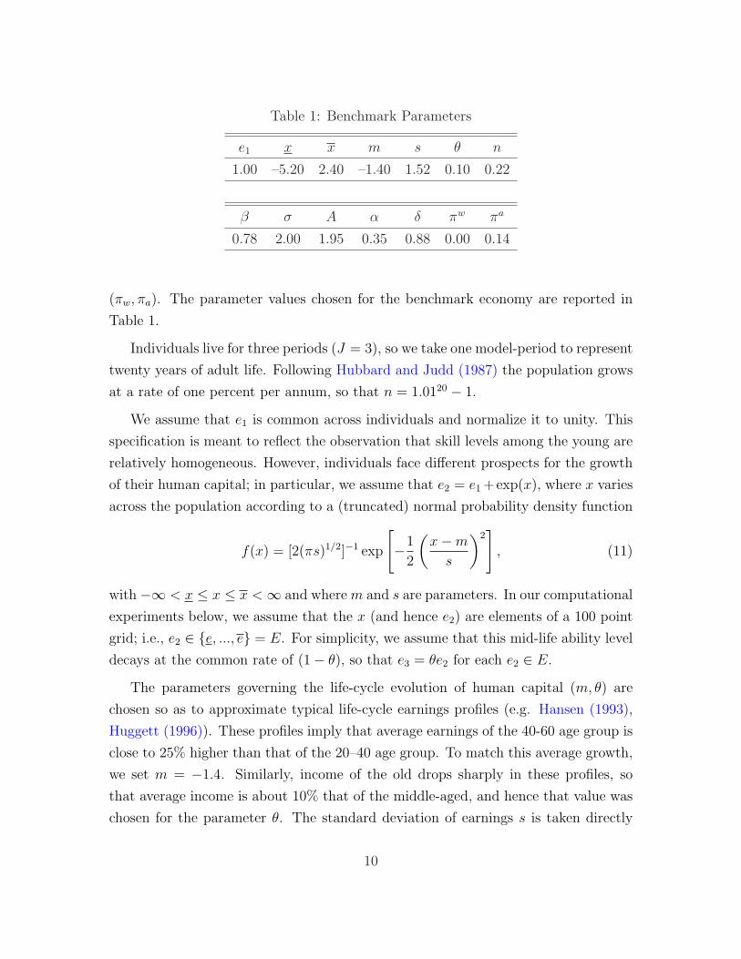
Table 1: Benchmark Parameters

e1 x x m s θ n

1.00 –5.20 2.40 –1.40 1.52 0.10 0.22

β σ A α δ πw πa

0.78 2.00 1.95 0.35 0.88 0.00 0.14

(πw, πa). The parameter values chosen for the benchmark economy are reported in

Table 1.

Individuals live for three periods (J = 3), so we take one model-period to represent

twenty years of adult life. Following Hubbard and Judd (1987) the population grows

at a rate of one percent per annum, so that n = 1.0120 − 1.

We assume that e1 is common across individuals and normalize it to unity. This

specification is meant to reflect the observation that skill levels among the young are

relatively homogeneous. However, individuals face different prospects for the growth

of their human capital; in particular, we assume that e2 = e1 +exp(x), where x varies

across the population according to a (truncated) normal probability density function

f(x) = [2(πs)1/2]−1 exp

[−1

2

(x−m

s

)2]

, (11)

with−∞ < x ≤ x ≤ x < ∞ and where m and s are parameters. In our computational

experiments below, we assume that the x (and hence e2) are elements of a 100 point

grid; i.e., e2 ∈ {e, ..., e} = E. For simplicity, we assume that this mid-life ability level

decays at the common rate of (1− θ), so that e3 = θe2 for each e2 ∈ E.

The parameters governing the life-cycle evolution of human capital (m, θ) are

chosen so as to approximate typical life-cycle earnings profiles (e.g. Hansen (1993),

Huggett (1996)). These profiles imply that average earnings of the 40-60 age group is

close to 25% higher than that of the 20–40 age group. To match this average growth,

we set m = −1.4. Similarly, income of the old drops sharply in these profiles, so

that average income is about 10% that of the middle-aged, and hence that value was

chosen for the parameter θ. The standard deviation of earnings s is taken directly

10

from PSID data.5 Starting with all households whose head is around 40 in 1980 (we

used a 5 year age band—from 38 to 42—because of sample size), we added labor

earnings until 1997 (after 1997 the survey is no longer yearly) and divided by the

number of years for which income wasn’t missing—we threw out individuals who’s

income was missing for 5 or more years. We then computed the standard deviation

of log earnings of that sample. We set s to the value found in the data, 1.52. Finally,

since we have 100 individuals representing percentile of that distribution, we chose

the lowest and highest values of income to be ± 2.5 standard deviations away from

the mean.

The subjective discount factor β is chosen to have a capital to output ratio of 3.0

in the benchmark economy. The annual discount factor which achieves this goal is

0.988, so that β = 0.998820. The coefficient of relative risk aversion σ is fixed at 2.0.

The scaling technology parameter A is chosen to make output in the benchmark

economy equal to one. We fix the annual rate of depreciation of capital at 0.10, so

that δ = 1 − (1 − 0.1)20, and set α to 0.35, the capital share of total income in the

data, which produces an annual interest rate equal to 4.6%.

The parameter πw measures the degree to which creditors can recoup debt via

wage garnishment, should a debtor choose to default. In the United States, Federal

law stipulates that a minimum of 75% of wages or 30 times the Federal minimum

hourly wage per week, whichever is higher, be exempt from garnishment. Some states

(Texas, Pennsylvania, Alaska, South Dakota and Florida) prohibit wage garnishment

entirely; see Fay et al. (2002). Of course, legal stipulations are one thing and their

enforcement is another. In practice, it is likely very difficult for creditors to enforce

debt repayment through wage garnishment, even with a court order granting them

title to some of the debtor’s wage income. The primary reason for this state of affairs

likely resides in the fact that indentured servitude is legally prohibited in the United

States.6 Consequently, debtors can escape wage garnishment by reallocating time

to an activity that generates an excludable consumption flow (e.g., leisure or home

production), or perhaps to some underground activity. These considerations lead us

to set πw = 0.7

5We use the Cross National Equivalent Files (CNEF) produced by the Department of PolicyAnalysis and Management at Cornell University.

6This was not always the case; see Galenson (1981).7As discussed in Section 4, our results are robust to changes in this parameter value as long as

11

Debtors have a more difficult time protecting their physical and financial assets

(relative to their human capital) from seizure by creditors. Kehoe and Levine (2001)

effectively assume πa = 1.00, so that creditors can seize all assets (in value up to

the amount owed). This restriction effectively excludes defaulters from future par-

ticipation in financial markets. In reality, the ability of creditors to seize property

is limited. Even in the absence of personal bankruptcy laws, courts will typically

limit the amount of assets that can be seized (especially if their seizure results in

‘below subsistence’ living standards). In addition, since the Bankruptcy Reform Act

of 1978, generous exemptions for ‘rich debtors’ have been possible. This law allowed

bankrupts to keep $7500 in homestead equity and $4000 in non-homestead property

from creditors. In 1994, these exemption levels were doubled. Furthermore, many

states have adopted even more generous exemption levels (e.g., an unlimited home-

stead equity feature is not uncommon). Consequently, debtors can to some extent

avoid asset seizure by allocating their assets and savings to these exempt categories.

In one extreme case, we could set πa = 0, but this would result in a non-negative net

worth constraint since debtors could default with impunity. While this case represents

the norm commonly adopted in the literature, it is also somewhat counterfactual; in

reality, a considerable amount of unsecured debt is extended by creditors. For the

benchmark economy studied here, πa primarily determines the level of the debt that

individuals can obtain. We thus calibrate πa to replicate the average debt to income

ratio observed in the data. Livshits et al. (2007) report that the ratio of unsecured

debt to disposable income over the 1995 to 1999 period was 8.4%. Since disposable

income over the same period was 72.7% of GDP, we set πa = 0.14 to achieve a target

debt to income ratio of 6.1%. To put the level of asset garnishment in perspective, it

is useful to think of the implicit interest rate that individuals face upon default. In

the benchmark economy, the level of πa implies that individuals who defaulted in the

past keep around 65% of their interest income.8

the same calibration strategy is used.8This level is substantially higher than the 25% used in Rojas and Urrutia (2007). One reason

is that they calibrate their economy under a social security system and perform the opposite ex-periment, i.e. the removal of the system. As we will see in the next section, debt levels are muchlower under a social security system. Hence they need a harsher punishment to sustain any givenlevel of debt, even if their target debt/income ratio is about half of ours—this is simply becausethe level of unsecured debt has increased substantially from the 80’s—the period they use for theircalibration—to the late 90’s.

12

3.2 Welfare Measures

A government policy regime essentially boils down to the choice of τ . Let cj(x, τ) for

j = 1, 2, 3 be the equilibrium consumption allocation for a type x individual under

regime τ and define the function:

W (λ, τ) =

∫ 3∑j=1

βj−1u((1 + λ)cj(x, τ)

)df(x).

We interpret W (0, τ) as the ranking that a ‘representative’ individual (behind the

veil of ignorance) would attach to living in an economy under policy regime τ .

Our benchmark economy is that of a laissez-faire regime; i.e., τ = 0. Our ‘com-

pensating variation’ measure λ is computed according to:

W (λ, τ) = W (0, 0).

That is, λ has the interpretation of being the fraction of per-period consumption

that one would have to compensate the representative individual for moving from the

laissez-faire policy regime to the policy regime τ . Accordingly, positive values imply

that a representative individual would rather live in the laissez-faire world, and a

negative value implies that a representative individual would rather live in a world

with the alternative policy regime.

Below, we also present compensating variations conditional on ability. In this

case, redefine the function

W (x, λ, τ) =3∑

j=1

βj−1u((1 + λ)cj(x, τ)

)

and compute the type-contingent compensating variation λ(x) according to:

W (x, λ, τ) = W (x, 0, 0).

3.3 Properties of the Calibrated Model

In Table 2, we report a number of statistics produced by our calibrated model across

a range of parameter values for πa (where πa = 0.14 corresponds to the benchmark

13

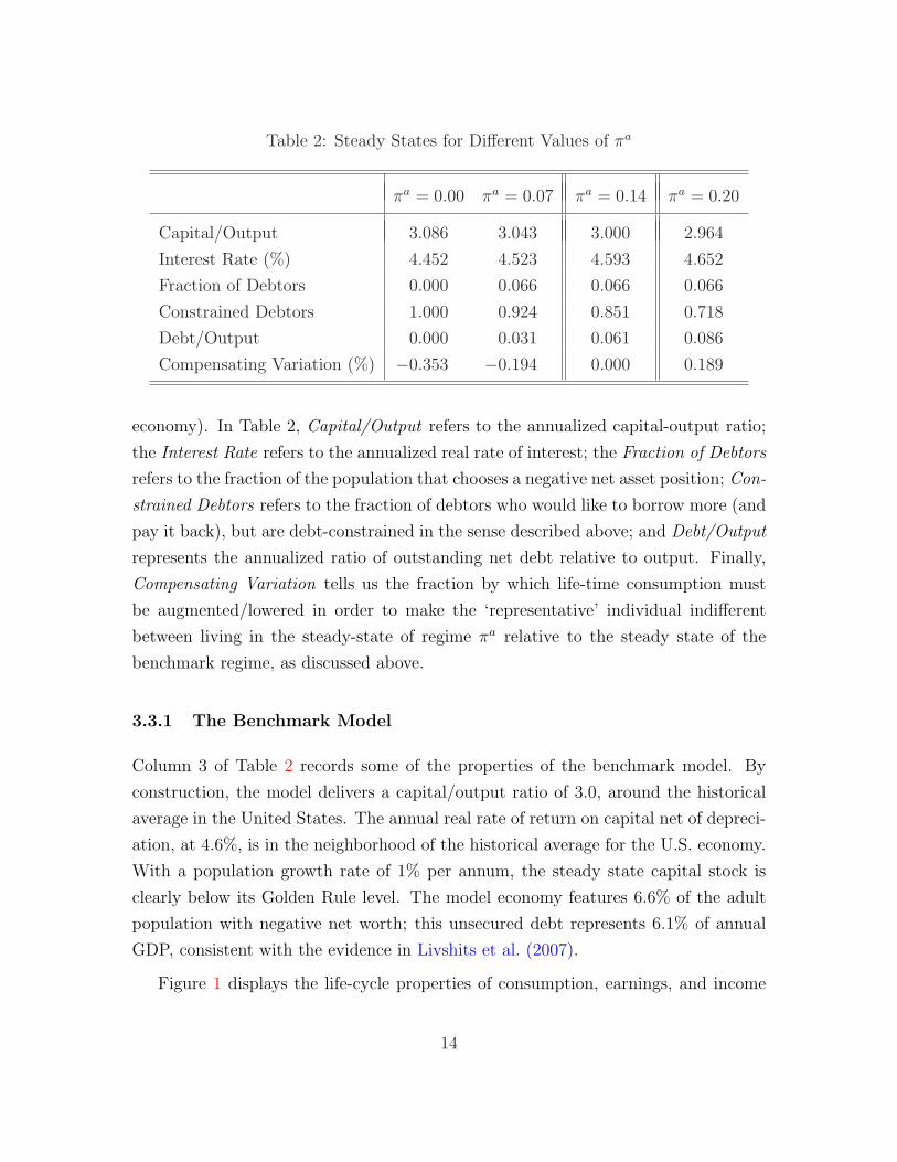
Table 2: Steady States for Different Values of πa

πa = 0.00 πa = 0.07 πa = 0.14 πa = 0.20

Capital/Output 3.086 3.043 3.000 2.964

Interest Rate (%) 4.452 4.523 4.593 4.652

Fraction of Debtors 0.000 0.066 0.066 0.066

Constrained Debtors 1.000 0.924 0.851 0.718

Debt/Output 0.000 0.031 0.061 0.086

Compensating Variation (%) −0.353 −0.194 0.000 0.189

economy). In Table 2, Capital/Output refers to the annualized capital-output ratio;

the Interest Rate refers to the annualized real rate of interest; the Fraction of Debtors

refers to the fraction of the population that chooses a negative net asset position; Con-

strained Debtors refers to the fraction of debtors who would like to borrow more (and

pay it back), but are debt-constrained in the sense described above; and Debt/Output

represents the annualized ratio of outstanding net debt relative to output. Finally,

Compensating Variation tells us the fraction by which life-time consumption must

be augmented/lowered in order to make the ‘representative’ individual indifferent

between living in the steady-state of regime πa relative to the steady state of the

benchmark regime, as discussed above.

3.3.1 The Benchmark Model

Column 3 of Table 2 records some of the properties of the benchmark model. By

construction, the model delivers a capital/output ratio of 3.0, around the historical

average in the United States. The annual real rate of return on capital net of depreci-

ation, at 4.6%, is in the neighborhood of the historical average for the U.S. economy.

With a population growth rate of 1% per annum, the steady state capital stock is

clearly below its Golden Rule level. The model economy features 6.6% of the adult

population with negative net worth; this unsecured debt represents 6.1% of annual

GDP, consistent with the evidence in Livshits et al. (2007).

Figure 1 displays the life-cycle properties of consumption, earnings, and income

14

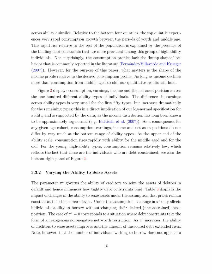
across ability quintiles. Relative to the bottom four quintiles, the top quintile experi-

ences very rapid consumption growth between the periods of youth and middle age.

This rapid rise relative to the rest of the population is explained by the presence of

the binding debt constraints that are more prevalent among this group of high-ability

individuals. Not surprisingly, the consumption profiles lack the ‘hump-shaped’ be-

havior that is commonly reported in the literature (Fernandez-Villaverde and Krueger

(2007)). However, for the purpose of this paper, what matters is the shape of the

income profile relative to the desired consumption profile. As long as income declines

more than consumption from middle-aged to old, our qualitative results will hold.

Figure 2 displays consumption, earnings, income and the net asset position across

the one hundred different ability types of individuals. The differences in earnings

across ability types is very small for the first fifty types, but increases dramatically

for the remaining types; this in a direct implication of our log-normal specification for

ability, and is supported by the data, as the income distribution has long been known

to be approximately log-normal (e.g. Battistin et al. (2007)). As a consequence, for

any given age cohort, consumption, earnings, income and net asset positions do not

differ by very much at the bottom range of ability types. At the upper end of the

ability scale, consumption rises rapidly with ability for the middle aged and for the

old. For the young, high-ability types, consumption remains relatively low, which

reflects the fact that these are the individuals who are debt-constrained; see also the

bottom right panel of Figure 2.

3.3.2 Varying the Ability to Seize Assets

The parameter πa governs the ability of creditors to seize the assets of debtors in

default and hence influences how tightly debt constraints bind. Table 3 displays the

impact of changes in the ability to seize assets under the assumption that prices remain

constant at their benchmark levels. Under this assumption, a change in πa only affects

individuals’ ability to borrow without changing their desired (unconstrained) asset

position. The case of πa = 0 corresponds to a situation where debt constraints take the

form of an exogenous non-negative net worth restriction. As πa increases, the ability

of creditors to seize assets improves and the amount of unsecured debt extended rises.

Note, however, that the number of individuals wishing to borrow does not appear to

15

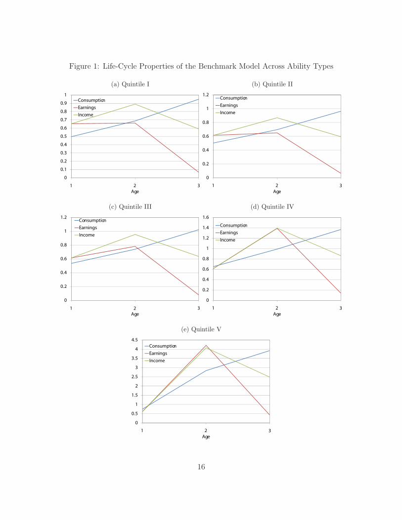
Figure 1: Life-Cycle Properties of the Benchmark Model Across Ability Types

(a) Quintile I

0 5

0.6

0.7

0.8

0.9

1Consumption

Earnings

Income

0

0.1

0.2

0.3

0.4

0.5

3

Age

1 2

(b) Quintile II

0 6

0.8

1

1.2Consumption

Earnings

Income

0

0.2

0.4

0.6

3

Age

1 2

(c) Quintile III

0 6

0.8

1

1.2Consumption

Earnings

Income

0

0.2

0.4

0.6

3

Age

1 2

(d) Quintile IV

0 8

1

1.2

1.4

1.6

Consumption

Earnings

Income

0

0.2

0.4

0.6

0.8

3

Age

1 2

(e) Quintile V

2.5

3

3.5

4

4.5

Consumption

Earnings

Income

0

0.5

1

1.5

2

3

Age

1 2

16

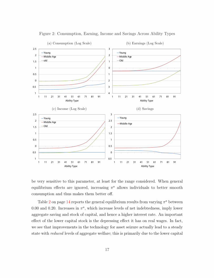
Figure 2: Consumption, Earning, Income and Savings Across Ability Types

(a) Consumption (Log Scale)

1

1.5

2

2.5

Young

Middle Age

old

1

0.5

0

0.5

1 11 21 31 41 51 61 71 81 91

Ability Type

(b) Earnings (Log Scale)

0

1

2

3

Young

Middle Age

Old

4

3

2

1

1 11 21 31 41 51 61 71 81 91

Ability Type

(c) Income (Log Scale)

1

1.5

2

2.5

Young

Middle Age

Old

1

0.5

0

0.5

1 11 21 31 41 51 61 71 81 91

Ability Type

(d) Savings

1.5

2

2.5

3

Young

Middle Age

0.5

0

0.5

1

1 11 21 31 41 51 61 71 81 91

Ability Type

be very sensitive to this parameter, at least for the range considered. When general

equilibrium effects are ignored, increasing πa allows individuals to better smooth

consumption and thus makes them better off.

Table 2 on page 14 reports the general equilibrium results from varying πa between

0.00 and 0.20. Increases in πa, which increase levels of net indebtedness, imply lower

aggregate saving and stock of capital, and hence a higher interest rate. An important

effect of the lower capital stock is the depressing effect it has on real wages. In fact,

we see that improvements in the technology for asset seizure actually lead to a steady

state with reduced levels of aggregate welfare; this is primarily due to the lower capital

17

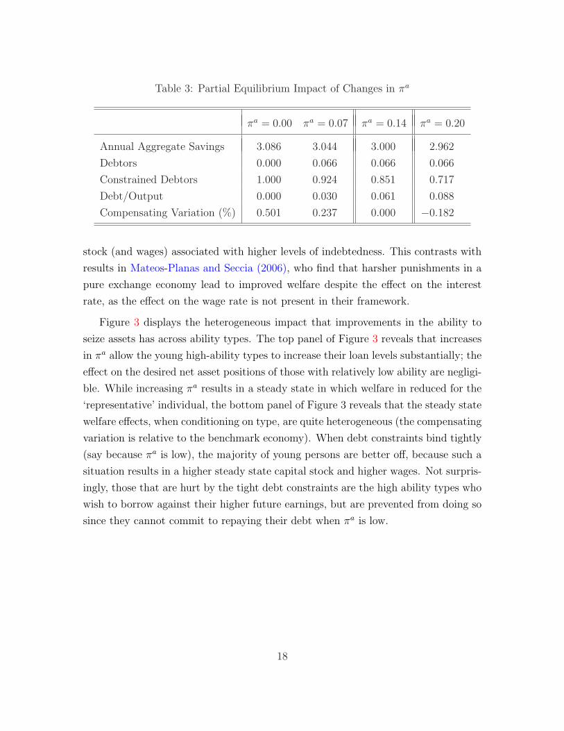
Table 3: Partial Equilibrium Impact of Changes in πa

πa = 0.00 πa = 0.07 πa = 0.14 πa = 0.20

Annual Aggregate Savings 3.086 3.044 3.000 2.962

Debtors 0.000 0.066 0.066 0.066

Constrained Debtors 1.000 0.924 0.851 0.717

Debt/Output 0.000 0.030 0.061 0.088

Compensating Variation (%) 0.501 0.237 0.000 −0.182

stock (and wages) associated with higher levels of indebtedness. This contrasts with

results in Mateos-Planas and Seccia (2006), who find that harsher punishments in a

pure exchange economy lead to improved welfare despite the effect on the interest

rate, as the effect on the wage rate is not present in their framework.

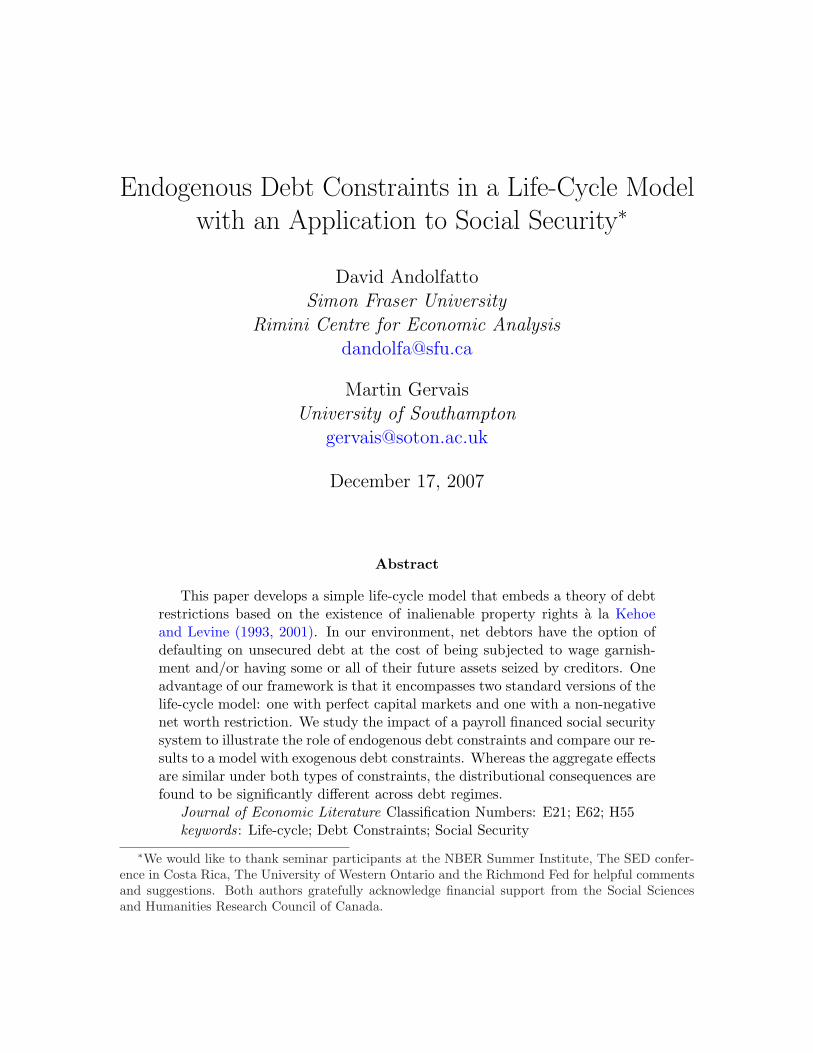
Figure 3 displays the heterogeneous impact that improvements in the ability to

seize assets has across ability types. The top panel of Figure 3 reveals that increases

in πa allow the young high-ability types to increase their loan levels substantially; the

effect on the desired net asset positions of those with relatively low ability are negligi-

ble. While increasing πa results in a steady state in which welfare in reduced for the

‘representative’ individual, the bottom panel of Figure 3 reveals that the steady state

welfare effects, when conditioning on type, are quite heterogeneous (the compensating

variation is relative to the benchmark economy). When debt constraints bind tightly

(say because πa is low), the majority of young persons are better off, because such a

situation results in a higher steady state capital stock and higher wages. Not surpris-

ingly, those that are hurt by the tight debt constraints are the high ability types who

wish to borrow against their higher future earnings, but are prevented from doing so

since they cannot commit to repaying their debt when πa is low.

18

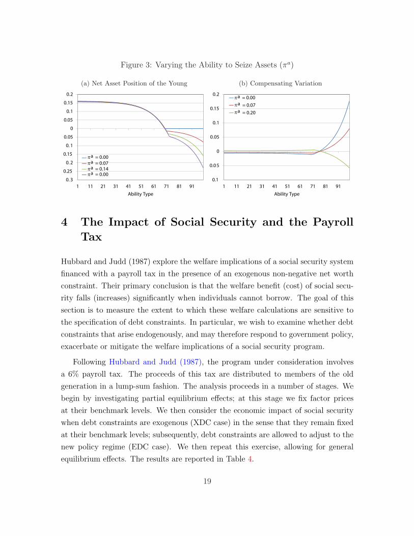
Figure 3: Varying the Ability to Seize Assets (πa)

(a) Net Asset Position of the Young

0 05

0

0.05

0.1

0.15

0.2

0. 3

0.25

0. 2

0.15

0. 1

0.05

1 11 21 31 41 51 61 71 81 91

Ability Type

π = 0.00a

π = 0.00a

π = 0.07a

π = 0.14a

(b) Compensating Variation

0 05

0.1

0.15

0.2π = 0.00

= 0.07

= 0.20

0.1

0.0 5

0

0.05

1 11 21 31 41 51 61 71 81 91

Ability Type

a

π a

π a

4 The Impact of Social Security and the Payroll

Tax

Hubbard and Judd (1987) explore the welfare implications of a social security system

financed with a payroll tax in the presence of an exogenous non-negative net worth

constraint. Their primary conclusion is that the welfare benefit (cost) of social secu-

rity falls (increases) significantly when individuals cannot borrow. The goal of this

section is to measure the extent to which these welfare calculations are sensitive to

the specification of debt constraints. In particular, we wish to examine whether debt

constraints that arise endogenously, and may therefore respond to government policy,

exacerbate or mitigate the welfare implications of a social security program.

Following Hubbard and Judd (1987), the program under consideration involves

a 6% payroll tax. The proceeds of this tax are distributed to members of the old

generation in a lump-sum fashion. The analysis proceeds in a number of stages. We

begin by investigating partial equilibrium effects; at this stage we fix factor prices

at their benchmark levels. We then consider the economic impact of social security

when debt constraints are exogenous (XDC case) in the sense that they remain fixed

at their benchmark levels; subsequently, debt constraints are allowed to adjust to the

new policy regime (EDC case). We then repeat this exercise, allowing for general

equilibrium effects. The results are reported in Table 4.

19

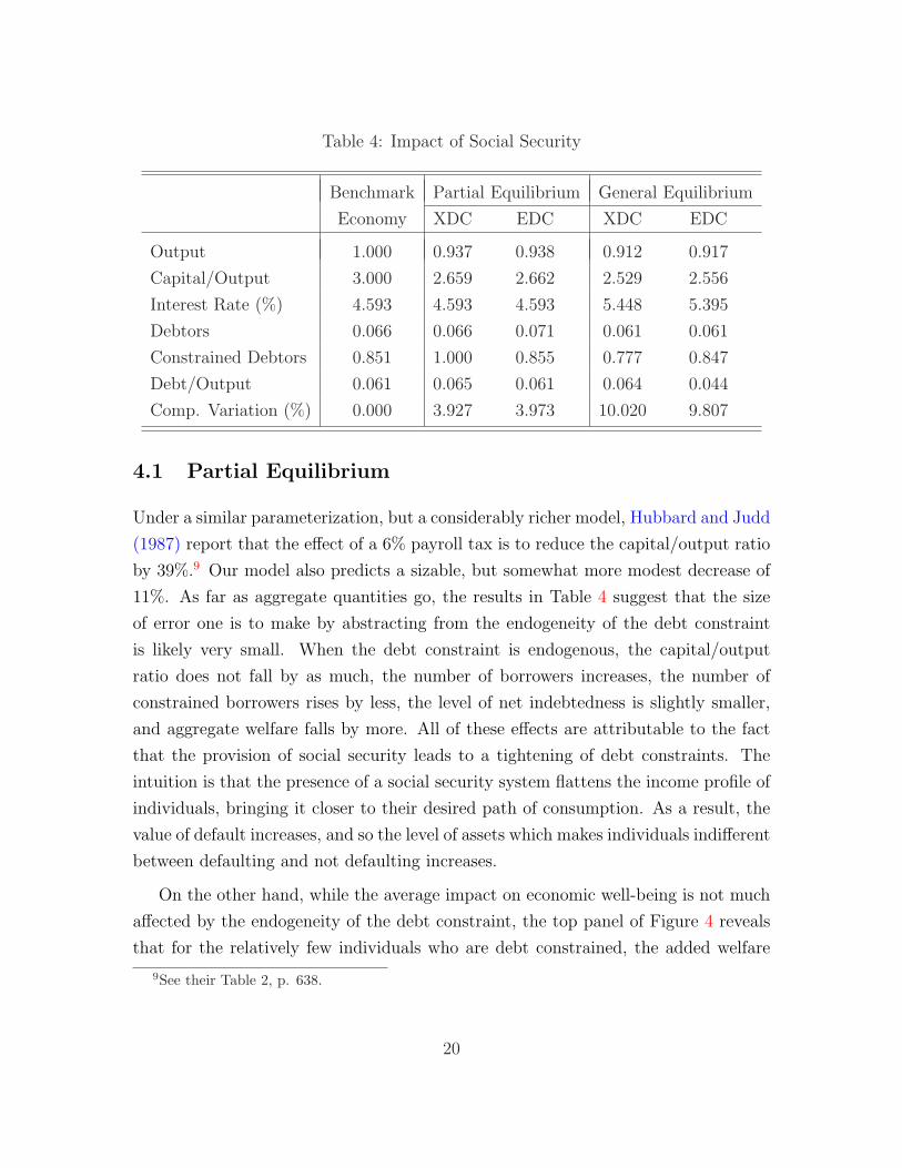
Table 4: Impact of Social Security

Benchmark Partial Equilibrium General Equilibrium

Economy XDC EDC XDC EDC

Output 1.000 0.937 0.938 0.912 0.917

Capital/Output 3.000 2.659 2.662 2.529 2.556

Interest Rate (%) 4.593 4.593 4.593 5.448 5.395

Debtors 0.066 0.066 0.071 0.061 0.061

Constrained Debtors 0.851 1.000 0.855 0.777 0.847

Debt/Output 0.061 0.065 0.061 0.064 0.044

Comp. Variation (%) 0.000 3.927 3.973 10.020 9.807

4.1 Partial Equilibrium

Under a similar parameterization, but a considerably richer model, Hubbard and Judd

(1987) report that the effect of a 6% payroll tax is to reduce the capital/output ratio

by 39%.9 Our model also predicts a sizable, but somewhat more modest decrease of

11%. As far as aggregate quantities go, the results in Table 4 suggest that the size

of error one is to make by abstracting from the endogeneity of the debt constraint

is likely very small. When the debt constraint is endogenous, the capital/output

ratio does not fall by as much, the number of borrowers increases, the number of

constrained borrowers rises by less, the level of net indebtedness is slightly smaller,

and aggregate welfare falls by more. All of these effects are attributable to the fact

that the provision of social security leads to a tightening of debt constraints. The

intuition is that the presence of a social security system flattens the income profile of

individuals, bringing it closer to their desired path of consumption. As a result, the

value of default increases, and so the level of assets which makes individuals indifferent

between defaulting and not defaulting increases.

On the other hand, while the average impact on economic well-being is not much

affected by the endogeneity of the debt constraint, the top panel of Figure 4 reveals

that for the relatively few individuals who are debt constrained, the added welfare

9See their Table 2, p. 638.

20

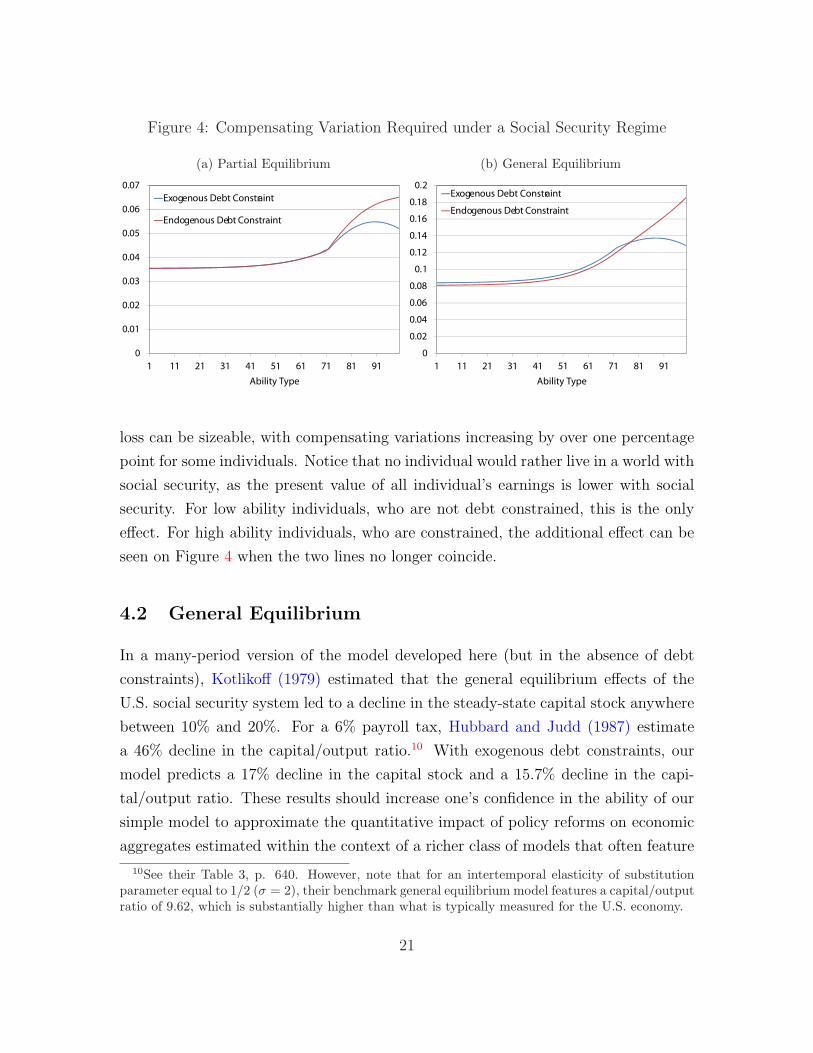
Figure 4: Compensating Variation Required under a Social Security Regime

(a) Partial Equilibrium

0.04

0.05

0.06

0.07

Exogenous Debt Constraint

Endogenous Debt Constraint

0

0.01

0.02

0.03

1 11 21 31 41 51 61 71 81 91

Ability Type

(b) General Equilibrium

0 1

0.12

0.14

0.16

0.18

0.2Exogenous Debt Constraint

Endogenous Debt Constraint

0

0.02

0.04

0.06

0.08

0.1

1 11 21 31 41 51 61 71 81 91

Ability Type

loss can be sizeable, with compensating variations increasing by over one percentage

point for some individuals. Notice that no individual would rather live in a world with

social security, as the present value of all individual’s earnings is lower with social

security. For low ability individuals, who are not debt constrained, this is the only

effect. For high ability individuals, who are constrained, the additional effect can be

seen on Figure 4 when the two lines no longer coincide.

4.2 General Equilibrium

In a many-period version of the model developed here (but in the absence of debt

constraints), Kotlikoff (1979) estimated that the general equilibrium effects of the

U.S. social security system led to a decline in the steady-state capital stock anywhere

between 10% and 20%. For a 6% payroll tax, Hubbard and Judd (1987) estimate

a 46% decline in the capital/output ratio.10 With exogenous debt constraints, our

model predicts a 17% decline in the capital stock and a 15.7% decline in the capi-

tal/output ratio. These results should increase one’s confidence in the ability of our

simple model to approximate the quantitative impact of policy reforms on economic

aggregates estimated within the context of a richer class of models that often feature

10See their Table 3, p. 640. However, note that for an intertemporal elasticity of substitutionparameter equal to 1/2 (σ = 2), their benchmark general equilibrium model features a capital/outputratio of 9.62, which is substantially higher than what is typically measured for the U.S. economy.

21

many periods, bequests, and uninsured idiosyncratic uncertainty.

As is consistent with the results reported in Hubbard and Judd (1987), the adverse

consequences of a payroll-tax financed social security program in the presence of debt

constraints is greatly exacerbated when general equilibrium forces come into play.

However, the aggregate differences that arise owing to the endogeneity of the debt

constraints remain small. With endogenous debt constraints, the steady state level

of indebtedness in the economy does shrink considerably (the debt/output ratio is

30% lower in this case), owing to the tightening of credit market conditions. But

the impact that this difference makes on the aggregate capital stock is rather small,

with endogeneity resulting in a capital stock that is ‘only’ 1.6% larger. The average

welfare differences that arise owing to endogeneity of the debt constraint are also

quite small, although note that general equilibrium reverses the partial equilibrium

results reported above; i.e., with endogenous debt constraints, steady state welfare

does not fall by as much under general equilibrium as it does when debt constraints

are exogenous (the reverse is true under partial equilibrium).

Once again, however, we note that these aggregate implications mask a consid-

erable amount of differences that occur at the individual level. The bottom panel

of Figure 4 displays the compensating variations required across ability types un-

der general equilibrium for both exogenous and endogenous debt constraints. Since

we are only comparing utility across steady state, one must interpret these numbers

as whether an individual would rather live in an alternative world rather than live

in the world described by the benchmark economy. Evidently, the endogeneity of

the debt constraint leaves lower ability types better off relative to the case where

debt constraints are assumed to be exogenous. These individuals are not directly

affected by the increased tightness of the constraint and the resulting (relative) in-

crease in capital implies a higher return for their labor. The high ability individuals

also benefit from the increased return to labor, but these gains are swamped by the

tighter debt constraints that afflict this set of individuals. At the aggregate level,

this differential impact across ability types more or less washes out, leaving us with

the conclusion that in terms of aggregate measures of welfare, endogenizing the debt

constraint makes little difference.

22

4.3 Alternative Bankruptcy Code

Given a calibration strategy in which the debt to income ratio is kept constant, setting

πa to zero and choosing πw to achieve that level of debt results in the exact same

steady state as the benchmark economy. Furthermore, the results in this section are

essentially identical under this alternative calibration.

5 Conclusions

This paper investigates whether the welfare calculations usually found in the literature

with regard to the introduction of a social security system (eg. Hubbard and Judd

(1987)) are sensitive to the specification of the borrowing constraint. We develop

an overlapping generations model in which, in the spirit of Kehoe and Levine (1993),

debt restrictions arise endogenously due to the existence of inalienable property rights.

The legal structure we consider is one in which creditors lay claims to a fraction of a

defaulter’s assets (either current or future). Although an improvement in the ability

of creditors to seize assets helps debt constrained individuals to obtain credit, it also

lowers the level of the capital stock as well as the wage rate, leading to lower aggregate

welfare. This is in contrast to pure exchange economies, as in Mateos-Planas and

Seccia (2006), where the effect on wages does not arise.

The results of this paper suggest that if one is only interested in the aggregate

impact of social security, then an exogenous specification of the borrowing constraint

is not a bad approximation. Indeed, results in Rojas and Urrutia (2007) suggest that

our results generalize to economies where individuals face uninsurable idiosyncratic

uncertainty, not only in steady state but also during the transition. These aggregate

results, however, mask important heterogeneous effects at the individual level.

23

References

Alvarez, F. and U. J. Jermann (2000). Efficiency, equilibrium, and asset pricing with

risk of default. Econometrica 68 (4), 775–797.

Andolfatto, D. and M. Gervais (2006). Human capital investment and debt con-

straints. Review of Economic Dynamics 9 (1), 52–67.

Battistin, E., R. Blundell, and A. Lewbel (2007). Why is consumption more log

normal than income? Gibrat’s Law revisited. Institute for Fiscal Studies Working

Paper 08/07.

Bulow, J. and K. Rogoff (1989). Sovereign debt; Is to forgive to forget. American

Economnic Review 79 (1), 43–50.

Chatterjee, S., D. Corbae, M. Nakajima, and J.-V. Rıos-Rull (2007). A quantitative

theory of unsecured consumer credit with risk of default. Econometrica 75 (6),

1525–1589.

Fay, S., E. Hurst, and M. J. White (2002). The household bankruptcy decision.

American Economic Review 92 (3), 708–718.

Fernandez-Villaverde, J. and D. Krueger (2007). Consumption over the life cycle:

Facts from Consumer Expenditure Survey data. Review of Economics and Statis-

tics 89 (3), 552–565.

Galenson, D. W. (1981). The market evaluation of human capital: The case of

indentured servitude in colonial america. Journal of Political Economy 89 (3),

446–467.

Hansen, G. D. (1993). The cyclical and secular behaviour of the labour input: Com-

paring efficiency units and hours worked. Journal of Applied Economics 8 (1),

71–80.

Hubbard, G. R. and K. L. Judd (1987). Social security and individual welfare: Pre-

cautionary saving, borrowing constraints, and the payroll tax. American Economic

Review 77 (4), 630–646.

24

Huggett, M. (1996). Wealth distribution in life-cycle economies. Journal of Monetary

Economics 38 (3), 469–494.

Kehoe, T. J. and D. K. Levine (1993). Debt constrained asset markets. Review of

Economic Studies 60 (4), 865–888.

Kehoe, T. J. and D. K. Levine (2001). Liquidity constrained markets versus debt

constrained markets. Econometrica 69 (3), 575–598.

Kocherlakota, N. R. (1996). Implications of efficient risk sharing without commitment.

Review of Economic Studies 63 (4), 595–609.

Kotlikoff, L. J. (1979). Social security and equilibrium capital intensity. Quarterly

Journal of Economics 94, 233–253.

Krueger, D. and F. Perri (2005). Public versus private risk sharing. Unpublished

manuscript.

Livshits, I., J. MacGee, and M. Tertilt (2007). Consumer bankruptcy: A fresh start.

American Economic Review 97 (1), 402–418.

Mateos-Planas, X. and G. Seccia (2006). Welfare implications of endogenous credit

limits with bankruptcy. Journal of Economic Dynamics & Control 30 (11), 2081–

2115.

Rojas, J. A. and C. Urrutia (2007). Social security reform with uninsurable income

risk and endogenous borrowing constraints. Forthcoming in Review of Economic

Dynamics.

25