Embed Size (px)
Citation preview

End-to-End Tracing Models:
Analysis and Unification
Jonathan Leavitt
Department of Computer Science
Brown University
May 5, 2014
i

Abstract
Many applications today require distributed systems to store and process massive amounts
of data. The complexity of these applications grows as the systems running them become more
complex, and as the applications require more systems in order to run. End-to-end tracing
is the process of following a request through the network of machines running one or more
distributed systems in order to aid in the maintenance, debugging, and optimization of the
systems. We will analyze the two primary models used for end-to-end tracing systems, the
span model and the event model. We will show that spans are the less powerful model through
a formal proof and a practical implementation of the proof, as well as discuss the consequences
of using the span model. We will finish by proposing a joint model that incorporates both spans
and events.
1

Contents
1 Introduction 3
1.1 Uses . . . . . . . . . . . . . . . . . . . . . . . . . . . . . . . . . . . . . . . . . . 3
2 Tracing Models 5
2.1 Spans . . . . . . . . . . . . . . . . . . . . . . . . . . . . . . . . . . . . . . . . . 5
2.2 Events . . . . . . . . . . . . . . . . . . . . . . . . . . . . . . . . . . . . . . . . . 8
3 The Span Model Is Less Powerful Than The Event Model 9
3.1 Proof That Events Are Fully Expressive And Spans Are Not . . . . . . . . . . . . 9
3.2 Proof By Reduction That Events Are More Powerful Than Spans . . . . . . . . . . 11
3.2.1 Proof . . . . . . . . . . . . . . . . . . . . . . . . . . . . . . . . . . . . . 11
3.2.2 Practical Implementation Of The Reduction . . . . . . . . . . . . . . . . . 14
4 Unification 17
4.1 Motivation . . . . . . . . . . . . . . . . . . . . . . . . . . . . . . . . . . . . . . . 17
4.2 X-Trace With Spans . . . . . . . . . . . . . . . . . . . . . . . . . . . . . . . . . . 20
4.2.1 Execution . . . . . . . . . . . . . . . . . . . . . . . . . . . . . . . . . . . 20
4.3 Results . . . . . . . . . . . . . . . . . . . . . . . . . . . . . . . . . . . . . . . . . 21
4.3.1 Differences . . . . . . . . . . . . . . . . . . . . . . . . . . . . . . . . . . 21
4.3.2 Example . . . . . . . . . . . . . . . . . . . . . . . . . . . . . . . . . . . 23
5 Conclusion 23
2

Figure 1: Simple depiction of the path taken through a system to service a request requiring mul-tiple processes’ cooperation (each lettered node in the graph represents a process in the system).Taken from [8].
1 Introduction
Many distributed systems have been created in recent years to store and process massive amounts
of data. These systems are extremely complex and require the careful coordination of several
processes1 to accomplish even simple tasks. Applications often rely on more than one of these
systems, considerably increasing the complexity. End-to-end tracing is the process of following a
particular request through this network of processes in order to gain more understanding into how
the system works and what may be going wrong, specifically with respect to the causal relation-
ships among different events and processes. The image in Figure 1, taken from Google’s Dapper
paper [8], provides a high level illustration of the type of information we seek when tracing dis-
tributed systems. The trace being displayed is of a simple web request from a user that requires
communication to multiple backend systems in order to service the request.
1.1 Uses
End-to-end tracing information is useful for debugging these systems because it provides an im-
portant axis of logging information that transcends the standard logging done by each process. In
addition to viewing logging information through the standard process and time axes, tracing pro-
vides a third axis based on requests. The ability to see exactly which processes were involved in
servicing a particular request, as well as the causal relationships among those processes, is invalu-
able in maintaining, debugging, and improving these systems.
1Note that these processes may be on the same machine or span across multiple machines.
3

Figure 2: A trace of an HDFS put operation created with HTrace (from HDFS-5275 [2]).
Additionally, end-to-end request tracing can be very useful for profiling and improving perfor-
mance of distributed systems. With a set of trace information for a system, one can see exactly
how much time the system is spending on various types of tasks and optimize appropriately. See
Figure 2 for a trace of a put request in a Hadoop Distributed Filesystem (HDFS) cluster created
using HTrace [3] and visualized using Zipkin’s [9] visualization tools; the image itself is taken
from HDFS-5274 [2].
With end-to-end tracing, damage control and preemptive performance tuning on one’s cluster
is significantly simplified. In lieu of GREP’ing log files in order to find anomalous behavior, one
can simply inspect visualizations of traces for faulty executions to find the problem. For example,
consider HBase, the column-oriented distributed database built on HDFS. An important part of
correctly configuring an HBase cluster is choosing a proper row-key schema. Rows in HBase are
sorted by their row-keys. Row-keys that are lexicographically close are kept physically close in the
4

cluster. If the row-key schema is poorly chosen, too many requests might be routed to a particular
machine which could become overloaded. While standard machine monitoring would detect an
overloaded machine in the cluster, it would only detect it once the machine is already overloaded.
With end-to-end tracing in the same situation, automated tools could analyze the tracing data and
see that a proportionally high percentage of requests are being routed through one machine and
suggest that perhaps the row-key scheme was poorly designed.
A very important feature of any tracing library is the ability to trace both within a system and
across systems. The more tracing coverage that exists across systems, the fewer ‘black holes’ there
are in the information collected, and the more useful the information becomes. It would thus be
beneficial to create or standardize one primary tracing model and library that would easily allow
the coalescence of tracing information collected from many different systems.
2 Tracing Models
There are many tracing implementations, including Dapper [8], HTrace [3], X-Trace [5], Accu-
mulo’s Cloudtrace [1], and Zipkin [9]. These libraries represent tracing information with different
models, and provide different APIs to the developer trying to instrument a system. HTrace and
Zipkin follow the model introduced in Dapper and represent the distributed computation as a tree
of spans, while X-Trace uses a model of logging a graph of events.
2.1 Spans
The span model was first introduced by Google [8], and has since found a fairly good mindshare,
with HTrace, Zipkin, and Cloudtrace all using the span model as the basis for their end-to-end
tracing systems.
The span model represents a computation as a collection of spans, each of which represents a
chunk of work in the computation. Because spans represent an interval of time in the computation,
they require a start and an end time. Additionally, each span has information on which other span
in the trace started it, representing the causality in the system. If SpanA started SpanB, SpanA
is called the parent of SpanB. In most systems, each span knows the identity of its parent with a
field storing the unique identifier of its parent.
5

A trace is a collection of spans that were created from the same computation. If we consider
each span as a node, and a parent relationship as a directed edge from the parent to the child, a trace
can be easily interpreted and understood as a graph. Because the parent relationship represents
causality, it is not possible for a cycle to exist in the graph. A cycle would transitively imply that
there is some event that caused itself, and also caused the event that caused it – a contradiction.
Thus span graphs are just trees with directed edges pointing from the root down toward the leaves.
An important part of the span model is that spans only have a single parent. Tracing systems
that use the span model generally keep a stack of the spans that have yet to be ‘stopped’. The span
at the top of the stack is the current span. When the current span, call it SpanA, is stopped, it is
delivered (generally to a database), and the next span in the stack, SpanA’s parent, is the new
current span. Such a stack would be impossible if spans could have multiple parents (what span
would be current after a span with two parents is popped?).
The stack is kept local to each thread so that parallel computations can be accurately repre-
sented. When a remote procedure call (RPC) is sent across the wire, a unique identifier for the
span that was current when the RPC was sent and the unique identifier for the entire trace is sent
along with the RPC (these identifiers are generally two sixty-four bit unsigned integers). When a
new span is started on the machine receiving the RPC, it sets its parent field to the identifier for the
span in the RPC and its overall trace identifier (the field for which all spans of the same trace share
the same value) to the trace identifier from the RPC. Figure 3 shows a pseudocode example, and
Figure 4 depicts the span graph that would be generated by the code in Figure 3.
The span implementation outlined above and used in the example in Figure 3 has a symmetry
problem. When several spans are started on the same machine, the stack is maintained and the
programmer using the tracing library can ‘pop’ spans indiscriminately. Once the computation
crosses to a new machine, the stack is lost and the programmer can no longer pop spans as he
could on one machine. This asymmetry could be solved by sending the entire stack along with
each RPC, but this is not feasible because the size of the metadata attached to each RPC would be
unbounded. Asymmetry is not necessarily a bad thing, but it can be confusing for the user.
The span model is easy to understand for the programmer using the model in order to instru-
ment a system. The single point of causality provides a call-stack type view of the computation
that is conceptually easy for the user of the library to understand. Unfortunately, the span model
6

// running on machine 1:
// assume doingWhatever has span identifier and trace identifier values// of 1 and 5 respectivelySpan doingWhatever = Trace.startSpan("doing whatever");
// assume ’sendPing’ has span identifier and trace identifier values// of 1 and 2. its parent span field would be 5 because// the doingWhatever span is its parent.Span sendPing = Trace.startSpan("sending ping");
// rpcPing would append the information (trace: 2,span: 1)// along with the RPC informationrpcPing();// end the spans and deliver them to some source for processing etc.sendPing.stop();doingWhatever.stop();
// running on machine 2:rpcReceivePing(RPC rpc) {
if (rpc.hasTracingInformation()) {// pingSpan’s trace id would be 2, its span id would// be randomly generated, and its parent id would be 1,// signifying that sendPing is its parent because// sendPing’s span id is 1uint64 traceId = rpc.getTraceId(); // 2uint64 spanId = rpc.getSpanId(); // 1Span pingSpan = Trace.startSpan(traceId=traceId,
parentSpanId=spanId,description="rcvd ping");
// do some stuff then stop and deliver the spanpingSpan.stop();
}}
Figure 3: Code example of how the span model might be integrated into a system’s RPC mecha-nism.
7

Figure 4: The span graph that would be generated by the code provided in Figure 3
is not powerful enough to represent all aspects of computation. In particular, the span model has
trouble representing certain types of computations, particularly those involving events that cannot
occur unless more than one other event has already taken place. Many asynchronous computations
have such dependencies.
Spans can represent any activation pattern because activation, by definition, is only some action
directly causing another action to occur (activating the new action). This activation relationship
can be represented by the parent relationship in the span model. Activation patterns do not fully
describe the nuances of many computations. For example, some action may only be activated
by one other action, but may actually depend on multiple other events occurring before it can be
activated. The span model cannot capture this relationship.
2.2 Events
The event model was originally used in the X-Trace end-to-end tracing system [5]. An X-Trace
event represents a single point in time in the computation. Causality is represented with edges
drawn between events. Edges can be drawn arbitrarily between any two events. Specifically,
an edge represents the happens-before relationship among arbitrary events, introduced by Leslie
Lamport, that signifies that some event could have influenced some other event [6].
Unlike the span model, in which a span can only have a single ‘parent’ that activated it, events
can have multiple incoming edges representing possible dependence on several other events oc-
8

curring. The ability to have multiple incoming edges for a particular event is beneficial because it
allows a more complete representation of some aspects of computations, particularly those involv-
ing the joining of multiple threads.
While the relationship among spans is pure activation, the relationship among events is the
more general concept of happens-before. All that happens-before represents is that some event
happened before some other event, but not necessarily that that ordering is always the case, or is
necessary to the computation. For example, EventA might happen before EventB, but there
may be some non-determinism and EventB might happen before EventA in some executions of
the program.
Dependency relationships are a subset of happens-before relationships. A dependency relation-
ship means that some event must happen before some other event in all executions. The differences
among activation, dependency and the happens-before relationship are subtle but extremely impor-
tant.
The downside of the X-Trace model is that it is not necessarily as intuitive for programmers to
use as the span model. The call-stack view that the span model provides has a level of simplicity
that the event model cannot match.
3 The Span Model Is Less Powerful Than The Event Model
We will show that the span model is strictly less powerful than the event model. We will do this two
ways. We will first prove that the event model is fully expressive and can accurately represent any
possible computation, and that the span model is not fully expressive. We will then prove that the
event model is more powerful than the span model by reducing from the span model to the event
model, and providing two examples (one contrived, one from a real system) of computations that
spans could not represent and events can represent. After discussing the reduction and examples,
we will describe our implementation of the reduction within the X-Trace tracing library.
3.1 Proof That Events Are Fully Expressive And Spans Are Not
Proof. An algorithm, whether it is executed with one or several processes, is fundamentally a
series of steps that, when taken, will produce some result. Assume we have an algorithm A we
9

want to carry out that requires n steps, S = {s1, s2, . . . , sn}. Assume without loss of generality
that s1 is just some generic start step that does not actually progress the computation. Also assume
that executing the steps in order (s1 → s2 → · · · → sn) would yield the desired result.
In the computation A, some of the steps depend on each other and some do not. That is to say
that some of the computation can be done in parallel. We could imagine creating a directed graph,
G, for which the nodes will be the set S = {s1, s2, . . . , sn}, and the set of edges, E, represents
dependence. That is to say that there is a directed edge from si to sj if and only if sj directly
depends on the results of si. In such a graph, there can be no self-loops because a step cannot
depend on itself (we will assume that the computation is deterministic and loops are unrolled).
Similarly, there can be no cycles in the graph at all because that would transitively imply that
a step depends on itself, which is a contradiction. We use the phrase ‘directly depends’ so that
for some arbitrary step si, the set {sj : (sj, si) ∈ E} represents the smallest possible subset of
S such that if all the steps in the subset are computed, it is possible to safely compute si. This
restriction makes the graph the transitive reduction of the dependency graph. For example, the
transitive reduction prevents all events from necessarily depending on s1 because no event in the
computation can occur until the computation has started. The idea for the transitive reduction was
taken from [4].
G is both directed and ayclic; G is a DAG (directed acyclic graph). To produce a trace rep-
resentable by the event model given the graph G, log one event for each node in S, and draw the
same directed edges between events that exist in G. That is, produce the same graph with events
that was made originally with the steps of the computation. This graph fully represents the compu-
tation’s dependency structure. Thus, every computation’s dependency structure can be completely
represented by the event model.
As a corollary to the above proof, note that the span model could not completely represent any
arbitrary computation because the graphs the span model produces can not have multiple incoming
edges representing dependency on multiple events that the DAG, G, created in the proof may have.
Thus the span model is not fully expressive.
10

3.2 Proof By Reduction That Events Are More Powerful Than Spans
3.2.1 Proof
Proof. To show that the event model is strictly more powerful than the span model, we will first
show a reduction from spans to events. Reproducing the span model with only events shows that
the event model is at least as powerful as the span model because it shows that any computation
the span model can represent can be represented by the event model via the reduction provided.
Second we will provide an example of a computation that the event model can represent and
the span model cannot represent. This example, combined with the reduction, will show that the
set of computations that the event model can represent is a strict superset of the set of computations
the span model can represent.
Reduction
The reduction from spans to events is as follows:
Whenever a span is started with spanID=S, log a special event that contains some metadata that
says this event represents the start of of the span with ID of S. The event must be timestamped, as
is generally the case for implementations of the event model. When the span is ended, log a similar
event with metadata that describes that the event represents the end of the span with ID of S. The
parent relationship critical to the span model can be represented in the event model by drawing
causality edges from each event representing the start of a span to the event representing the start
of the child span.
More simply, the reduction requires that for each span that is started and stopped, there are two
events created: one marking the start of the span, and the other marking the end of the span. The
parent relationship of the span model is maintained using the happens-before edges of the event
model.
Computation That Events Can Represent And Spans Cannot
As mentioned above, the second part of this proof involves an example of an execution that the
event model can represent and the span model cannot represent. This example can trivially be an
execution such as the following:
11

R
E1 E2
E3
In the image, each node is an event, and the directed edges are the causality edges. If E3 could
not occur without both E1 and E2 occurring, the multiple incoming edges to E3 are necessary to
accurately represent the computation’s dependencies. Because the span model represents causal-
ity with the singular parent relationship, the execution depicted in the image above could not be
accurately represented with the span model.
Instead, the resulting span graph would either look like:
R
E1 E2
E3
OR
12

R
E1 E2
E3
In the images above, each node represents a span, and the directed edges represent the par-
ent relationship (a directed edge from NodeA to NodeB means that NodeA is NodeB’s parent).
Note that in neither case is the computation accurately represented. These graphs serve as a good
example of how the parent relationship is not powerful enough to fully describe all executions.
Computations carried out in a multi-process environment require a more powerful construct than
just storing which part of the computation started each other part. Such a construct is the edge used
in the event model that does not represent pure causality, but instead represents the happens-before
relationship.
We modified the X-Trace tracing library to illustrate the reduction described, implementing a
span model with the events provided by X-Trace. We will describe the details of this practical
reduction later, as well as explain the results.
The contrived example provided above is sufficient for the purposes of our formal proof. On
the other hand, the question arises of whether such examples ever occur in real world systems. If
they do not, the difference in expressibility of spans and events is less important. Unfortunately for
the real world and fortunately for this document, such executions do occur in real world systems.
Such an example can be found in the Hadoop Distributed Filesystem (HDFS). See Figure 5 for
an image representing the relevant part of an HDFS get operation. Note the PacketReceiver
node that has two incoming edges from both a BlockSender event and a PacketReceiver
event. This is an example of an event that can only occur if two other events occur before it. A
span model of the same computation would not capture this dual dependence. The figure shows the
13

Figure 5: Portion of a trace of an HDFS get operation created with X-Trace.
portion of the request during which there is a pipelining of data blocks through a chain of nodes.
The dual dependence is showing that the PacketReceiver cannot receive an additional block
until its ACK has been received and another block is ready to be sent.
Thus we have shown, through a formal reduction and two counterexamples (one practical, one
contrived), that the span model is strictly less expressive than the event model.
3.2.2 Practical Implementation Of The Reduction
The goal of our practical implementation of the reduction described in the proof in the previous
section was to produce an API providing the semantics expected from a tracing library imple-
menting the span model using only the events in the X-Trace tracing library. This endeavor was
successful.
It is important to note that a non-goal of this practical implementation of the reduction was
the ability to use both spans and events together. For the purposes of the reduction it is sufficient
to only provide an API giving span model semantics. Thus this implementation does not work
properly if spans and events are used in the same trace.
As described in the proof above, the reduction logs a special startSpan event when a span
is started and a corresponding stopSpan event when the span is stopped. Without any type of
14

post-processing, the graph produced with this reduction is very difficult to interpret because there
are often edges connecting endSpan events to unrelated startSpan events. See Figure 6 for
the code used to create a trace with the reduction and the resulting event graph. Note that the
directions of the edges in the graph shown in Figure 6 are downward. The top three nodes in the
chain are the startSpan events and the bottom three nodes are the stopSpan events. The
event with label C89420ABC1A02A20 has an END SPAN field set to 11B2A8AE71AC2861,
signifying that it is the stopSpan event for the event labeled important work 2. The event
with the label 892E741A6CE28EE8 stops the event labeled important work 1, and the
event labeled 48D3D4568FDD424D stops the event labeled tracecreator.
Post-processing is required to complete the reduction and convert the graph of events into a
graph of spans. A span requires a start time, end time, unique span ID, trace ID, and a parent ID.
The ID of the entire trace is taken from the X-Trace ID for the trace. To create the spans given
the X-Trace events from the reduction, we find every startSpan event and its corresponding
endSpan event. The start time is the timestamp on the startSpan events and the end time is
the timestamp on the stopSpan event. The spanID is the event ID of the startSpan event.
The final remaining field necessary in order to have a complete span is the ID of the span’s
parent. Simply using the edges drawn between events is incorrect. Instead a traversal of the graph
is necessary. The code in Figure 7 illustrates how to find a span’s parent given its startSpan
event, and the event graph of the entire trace.
All the code does is traverse ‘up’ the edges from the event until an event is found that is neither
an endSpan event nor a startSpan event for which the corresponding stopSpan event was
already encountered in the traversal. The second part of the conditional prevents a span that was
stopped before the span for which we are finding a parent was started from being selected as the
span’s parent. Figure 8 illustrates a case for which the second part of the conditional is necessary.
In Figure 6, we see that for all of the startSpan events, the event directly ‘above’ it is its parent,
but that is not necessarily the case. Figure 8 is an example of such a trace.
Note the assumption that events only have one incoming edge. This assumption is only safe
because of the reduction, which prevents any event from having more than one incoming edge.
15
startSimpleTrace() {Span s = startSpan("tracecreator");importantWork1();s.stop();
}importantWork1() {
Span s = startSpan("important work 1");importantWork2();s.stop();
}importantWork2() {
Span s = startSpan("important work 2");sleepForSomeShortInterval();s.stop();
}
Figure 6: A simple trace created to demonstrate the results of the reduction (top) and a shortenedversion of the code that produced it (bottom). The dark grey lines in the top image connectstartSpan events with their corresponding stopSpan events.
16

def getParentId(startSpanEvent, eventGraph):if isRootEvent(startSpanEvent, eventGraph):
startSpanEvent.parentID = ROOT_SPAN_ID# edges = list of events this event is dependent oncur_event = startSpanEvent.edges[0]ends_seen = []
# Keep traversing ‘up’ the graph until we find a# startSpan event that has not been ‘stopped’ by an event# we have already encountered in the traversal.while (cur_event.isStopSpanEvent() or
cur_event.spanID inmap(lambda x : x.getIdOfSpanThisEventEnds(), ends_seen)):if cur_event.isStopSpanEvent():
ends_seen.append(cur_event)cur_event = cur_event.edge[0]
startSpanEvent.parentID = cur_event.spanID
Figure 7: Pseudocode necessary for the reduction from spans to events. The getParentIdfunction takes an event representing a startSpan and an eventGraph and appropriately setsstartSpanEvent’s parent span.
4 Unification
The span model and the event model both have unique advantages and disadvantages. While
spans cannot fully represent all types of computations, they provide a nice call-stack view of the
computation that experience has shown to be intuitive for users. Events on the other hand can
represent all types of computations (Section 3.1), but it is not always as obvious to users how to
best represent their computation with events. Additionally, the span model has a larger mindshare,
as evidenced by its use in Google’s Dapper (Dapper originally coined the term ‘span’) [8], Twitter’s
Zipkin [9], and Cloudera’s HTrace [3].
4.1 Motivation
The span model’s advantages (ease-of-use and greater mindshare in comparison to the event model)
do not outweigh its major disadvantage of not being able to fully express all aspects of a computa-
tion. Google’s paper titled, ‘Modeling the Parallel Execution of Black-Box Services’ [7] serves as
evidence of such a tradeoff’s practical implications. The paper attempts to estimate RPC latencies
17

Span s1 = startSpan("tracecreator");
Span s2 = startSpan("important work 1");
s2.stop();
Span s3 = startSpan("important work 1");
s3.stop();
s1.stop();
Figure 8: Top is an example of an event graph generated with the reduction for which a span’sparent is not always the event directly above it in the chain of causality. Bottom is the codegenerating the graph. The dark grey lines in the top image connect startSpan events with theircorresponding stopSpan events.
18

Figure 9: Image from Google’s paper, ‘Modeling the Parallel Execution of Black-Box Services’[7],showing the information they are working with (top), and the information they are seeking (bot-tom).
of computations that are “modeled by an ‘execution flow’, a direct acyclic graph.” Their goal is
to learn the execution flows by running statistical analysis on many thousands of traces produced
using Dapper [8] and its span model.
The graphic in Figure 9 shows the goal of the project behind the paper. Note how the top image
is the type of trace created with the span model and the bottom image more closely represents a
DAG that could easily be represented with events, and created with X-Trace. The paper describes
how using a lot of data can help obtain the necessary information to convert a span graph into
an event graph. Had Dapper [8] been built using the event model, the paper would never have
been written. The paper shows that the spans Google used in Dapper are not powerful enough to
represent the complex interactions that occur in their data centers.
It is possible to have both the simplicity of spans and the power of events. The ideal tracing
model would combine the flexibility and power of events, with the call-stack like simplicity of the
span model. The simplest solution is to produce a library that allows the user to use both spans and
events.
19

4.2 X-Trace With Spans
Our proposal is that events become the ‘assembly language’ of end-to-end tracing, and spans a
higher level construct built on top of events, similar to the reduction described in Section 3.2.2.
That reduction however is unsuitable for actual use because it breaks down if spans and events are
mixed.
Ideally the developer would instrument his system with spans whenever possible in order to
have the simplest and most understandable tracing information, and with events when the extra
expressive power is needed. When viewing traces, the developer should be able to view the trace at
a higher span level, and then drill deeper to view the more complex interactions represented with
the events. In the next section we describe our attempt to modify the X-Trace [5] tracing library to
include such features.
4.2.1 Execution
The X-Trace library has option fields, similar to those in many other networking services, that
allow easy extension of the protocol. Option fields are 〈key, value〉 pairs that are propagated along
with the standard X-Trace metadata. Option fields are the perfect place to store the information
necessary to properly add spans to the library.
The goal with the extension to the library is to allow the use of both spans and events in the
same trace. Unfortunately, the method used in the reduction in Section 3.2.2 is unsuitable because
the strategy of walking up the event graph in post-processing to find a span’s parent does not
work. Without the restriction of the reduction that prevents otherwise, events can be dependent on
multiple other events, and when that occurs it is not possible to deterministically walk up the graph
to find a parent because there are multiple paths that might lead to different answers for the span’s
parent.
To solve this problem, we chose to store the ID of the current span (if there is a current span) in
the current event’s option fields. Because the ‘current event’ is local to each thread and propagated
across machines, the correct span information is also kept thread-local and maintained across ma-
chines. The developer can use the existing X-Trace API as normal whenever he pleases, calling
the essential functions, such as logEvent, logMerge, joinContext, etc. When he wants to
20

begin a higher level span, he calls the startSpan function, which is presented (cleaned up for
clarity) in Figure 10. The startSpan function returns an XTraceSpan object, which stores
two ID’s: the ID of the span that was just created, and the ID of the span that was current before
that span was created (i.e. the newly created span’s parent). This object is necessary to stop the
span.
Stopping a span is as easy as calling the stop function on the XTraceSpan object returned
from the startSpan function. See Figure 11 for the code for the stopSpan function. The
function takes the XTraceSpan object representing the span to be stopped. The function first
logs an event with the END SPAN field set to the ID of the span stored in the XTraceSpan,
which effectively stops the span. Next, the function updates the current span option field in
the current event’s option fields to be the ID of the parent of the span being stopped, which makes
it possible to correctly start new spans in the future with the correct parent.
4.3 Results
4.3.1 Differences
There are some differences between the use of the X-Trace library with the span modifications and
a tracing library that natively supports spans. Namely, with X-Trace and the spans addition the
programmer cannot pop spans in the same manner that he can in a library, such as HTrace [3].
In HTrace, the library user can call a generic pop function that pops the current span and sets its
parent to be the current span, without having to keep a reference to the current span. In X-Trace
with spans, such actions are not possible, and the user of the library must maintain the ‘stack’ of
spans himself. Often however, the ‘stack’ is just the XTraceSpan objects that are created in each
new function called.
An example from a real world use of the span model provides evidence that developers do not
often use the ‘pop’ functionality mentioned above. Specifically, in the currently proposed patch
to integrate HTrace into HDFS, there are no cases in which a span is started but no references are
kept to the newly started span [2]. Thus, the requirement of X-Trace with spans that stipulates
that programmers must keep references to the spans they create in order to stop them does not
constitute a serious disadvantage with the library.
21

public static XTraceSpan startSpan(String description) {// Creates a new event with the description passed in,// and sets it as the current event.// does not yet send the report that// describes the event to the database.XTraceEvent event = XTraceContext.createEvent(description);
// Get the spanID of the current spanString curSpanString = getCurrentSpanFromOptionFields();// X-Trace events support arbitrary key-value pairs.// We insert in the event two mappings before we send the report// to the database.// The first signifies that this event is a special startSpan// event.// The second stores the spanID of this new span’s parent.event.put(START_SPAN_FIELDKEY, START_SPAN_STRING);event.put(PARENT_SPAN_FIELDKEY, curSpanString);event.sendReport();// Get the spanID of the span we just createdString newSpanString =
getFirstCurrentXTraceMetadata().getOpIdString();// and set it in the options for future spans// that might be started.setCurrentSpanInOptions(newSpanString);// Return a container object storing the ID of the// span that was just created, and the ID of the// span that was current before the new span// was created.// This object is necessary to properly stop the span.return new XTraceSpan(newSpanString, curSpanString);
}
Figure 10: The startSpan function that uses X-Trace’s option fields to store the current span’sID, and allows users to use spans and events in their systems.
22

public static void stopSpan(XTraceSpan toStop) {// Log the event signifying the end of the toStop// span.XTraceContext.logEvent(SPAN_AGENT,
NO_DESC_GIVEN,END_SPAN_FIELDKEY,toStop.getSpan());
// Set the option field storing the current span,// to be toStop’s parent (essentially a pop operation).setCurrentSpanInOptions(toStop.getSavedSpan());
}
Figure 11: The stopSpan function that takes an XTraceSpan, which stores the ID of the spanto be stopped and the ID of the parent span of the span to be stopped.
4.3.2 Example
As an example, we created a simple ‘chat’ program with two threads. The program simulates
two RPCs, with one saying ‘hello’ and the other replying back. We instrumented the example
program with X-Trace’s events and the spans we added to the X-Trace library to illustrate a trace
that contains both spans and events.
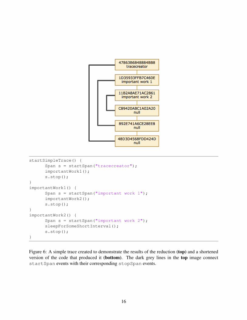
In Figure 12 and Figure 13 we can see the X-Trace event graph representing an execution of the
chat test program and the span graph created as a result of processing the event graph. Note that in
Figure 13, CR2 and CR1 stand for Chat Runnable 2 and Chat Runnable 1 respectively,
which are the two threads simulating the chat clients. recv1 is the second thread receiving the
first message, while send1 is the first thread sending the first message. The same applies for
resp2 and recv2.
Note that while the span representation shows the high level structure of the computation, the
specific details of how the greeting and response join together are missing. Figure 14 shows a
‘swim lane’ style representation of the trace that shows both the events and the spans.
5 Conclusion
End-to-end tracing systems are very useful for maintaining and debugging complicated distributed
systems and are consequently becoming more widely used among distributed systems developers.
23

As these tracing systems gain more traction, it is important to ensure the systems are built using
the correct models.
The span model is insufficient to represent all aspects of all computations and is thus not a
good choice for end-to-end tracing systems. While some developers may find the span model to be
sufficient for their current uses, they may encounter problems as their systems grow and produce
executions that cannot be modeled with spans. The event model is more powerful than the span
model, but is not as simple to use. Distributed systems developers should think carefully when
selecting a model for their own end-to-end tracing systems.
As just shown, it is possible to use both spans and events together when representing a compli-
cated computation. The spans can be used to show the activation hierarchy of the execution, and
the events can be used to represent the more intricate portions of the execution, as well as serving
as the lower level building block on which spans are constructed.
In the future it would be interesting to explore the visualizations and data analysis made pos-
sible with systems instrumented with spans and events. The visualization in Figure 14 is a good
example of the types of visualizations that could be created with spans and events. A tool that
initially shows a trace as only spans and allows the user to zoom in to see the events making up
those spans would be very useful in understanding systems’ executions.
24
Figure 12: X-Trace event graph for an execution of the test chat program.
chat
CR2 CR1
recv1 send1resp2 recv2
Figure 13: Span graph for an execution of the test chat program.
25

Figure 14: A ‘swimlane’ visualization that shows both the events and spans for an execution ofthe test chat program. Black dots are events and purple lines are edges between events. The greyrectangles represent spans. Each of the three large horizontal bars in the background represent thethree threads in the program. On top is the main thread, in the middle is the thread that receivesa message first, and on bottom is the thread that sends the first message. Note how the rectanglesrepresenting spans match the span tree in Figure 13. The nested lighter rectangles in the secondand third lanes are the spans created for sending and receiving the messages.
26

References
[1] Apache accumulo. http://accumulo.apache.org/.
[2] Elliot Clark. Hdfs-5274.
[3] Cloudera HTrace. http://github.com/cloudera/htrace.
[4] Rodrigo Fonseca. Improving Visibility of Distributed Systems through Execution Tracing. PhD thesis, EECS
Department, University of California, Berkeley, Dec 2008.
[5] Rodrigo Fonseca, George Porter, Randy Katz, Scott Shenker, and Ion Stoica. X-Trace: A Pervasive Network
Tracing Framework. In Proceedings of 4th USENIX Symposium on Networked Systems Design & Implementation
(NSDI 2007), April 2007.
[6] Leslie Lamport. Time, clocks, and the ordering of events in a distributed system. Commun. ACM, 21(7):558–565,
1978.
[7] Gideon Mann, Mark Sandler, Darja Krushevskaja, Sudipto Guha, and Eyal Even-Dar. Modeling the parallel exe-
cution of black-box services. In Proceedings of the 3rd Workshop on HotTopics in Cloud Computing, HotCloud,
Portland, Oregon, USA, 2011. USENIX Association.
[8] Benjamin H. Sigelman, Luiz Andre Barroso, Mike Burrows, Pat Stephenson, Manoj Plakal, Donald Beaver, Saul
Jaspan, and Chandan Shanbhag. Dapper, a large-scale distributed systems tracing infrastructure. Technical report,
Google, Inc., 2010.
[9] Twitter Zipkin. https://github.com/twitter/zipkin.
27


![On the relativistic unification of electricity and …arXiv:1111.7126v3 [physics.hist-ph] 19 Feb 2013 On the relativistic unification of electricity and magnetism Marco Mamone Capria∗and](https://img.pdfslide.us/doc/110x75/5fc972400ce514539242a038/on-the-relativistic-uniication-of-electricity-and-arxiv11117126v3-19-feb.jpg)
![On the relativistic unification of electricity and magnetism · arXiv:1111.7126v2 [physics.hist-ph] 18 Jul 2012 On the relativistic unification of electricity and magnetism Marco](https://img.pdfslide.us/doc/110x75/5b5adf3e7f8b9a302a8cbeb8/on-the-relativistic-unication-of-electricity-and-magnetism-arxiv11117126v2.jpg)