End-to-End Differentiable Adversarial Imitation Learningproceedings.mlr.press/v70/baram17a/baram17a.pdf · End-to-End Differentiable Adversarial Imitation Learning 2.3. Generative

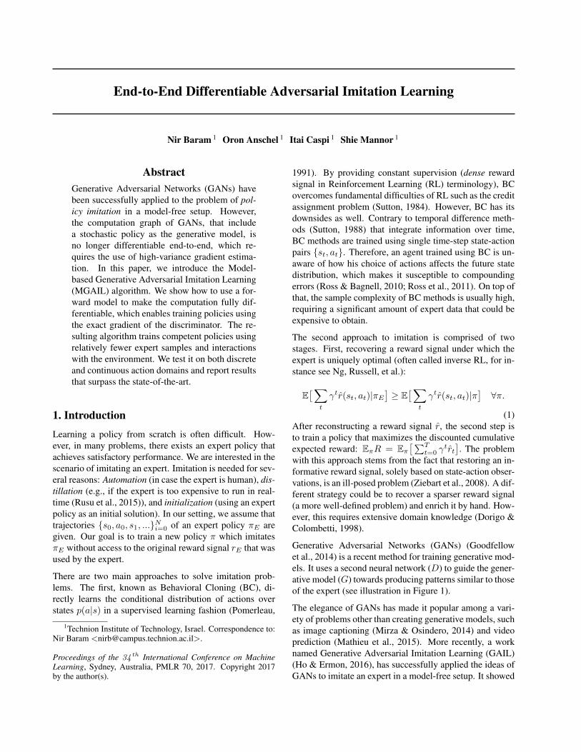
End-to-End Differentiable Adversarial Imitation Learning

Nir Baram 1 Oron Anschel 1 Itai Caspi 1 Shie Mannor 1

AbstractGenerative Adversarial Networks (GANs) havebeen successfully applied to the problem of pol-icy imitation in a model-free setup. However,the computation graph of GANs, that includea stochastic policy as the generative model, isno longer differentiable end-to-end, which re-quires the use of high-variance gradient estima-tion. In this paper, we introduce the Model-based Generative Adversarial Imitation Learning(MGAIL) algorithm. We show how to use a for-ward model to make the computation fully dif-ferentiable, which enables training policies usingthe exact gradient of the discriminator. The re-sulting algorithm trains competent policies usingrelatively fewer expert samples and interactionswith the environment. We test it on both discreteand continuous action domains and report resultsthat surpass the state-of-the-art.

1. IntroductionLearning a policy from scratch is often difficult. How-ever, in many problems, there exists an expert policy thatachieves satisfactory performance. We are interested in thescenario of imitating an expert. Imitation is needed for sev-eral reasons: Automation (in case the expert is human), dis-tillation (e.g., if the expert is too expensive to run in real-time (Rusu et al., 2015)), and initialization (using an expertpolicy as an initial solution). In our setting, we assume thattrajectories {s0, a0, s1, ...}Ni=0 of an expert policy πE aregiven. Our goal is to train a new policy π which imitatesπE without access to the original reward signal rE that wasused by the expert.

There are two main approaches to solve imitation prob-lems. The first, known as Behavioral Cloning (BC), di-rectly learns the conditional distribution of actions overstates p(a|s) in a supervised learning fashion (Pomerleau,

1Technion Institute of Technology, Israel. Correspondence to:Nir Baram <[email protected]>.

Proceedings of the 34 th International Conference on MachineLearning, Sydney, Australia, PMLR 70, 2017. Copyright 2017by the author(s).

1991). By providing constant supervision (dense rewardsignal in Reinforcement Learning (RL) terminology), BCovercomes fundamental difficulties of RL such as the creditassignment problem (Sutton, 1984). However, BC has itsdownsides as well. Contrary to temporal difference meth-ods (Sutton, 1988) that integrate information over time,BC methods are trained using single time-step state-actionpairs {st, at}. Therefore, an agent trained using BC is un-aware of how his choice of actions affects the future statedistribution, which makes it susceptible to compoundingerrors (Ross & Bagnell, 2010; Ross et al., 2011). On top ofthat, the sample complexity of BC methods is usually high,requiring a significant amount of expert data that could beexpensive to obtain.

The second approach to imitation is comprised of twostages. First, recovering a reward signal under which theexpert is uniquely optimal (often called inverse RL, for in-stance see Ng, Russell, et al.):

E[∑

t

γtr(st, at)|πE]≥ E

[∑t

γtr(st, at)|π]∀π.

(1)After reconstructing a reward signal r, the second step isto train a policy that maximizes the discounted cumulativeexpected reward: EπR = Eπ

[∑Tt=0 γ

trt]. The problem

with this approach stems from the fact that restoring an in-formative reward signal, solely based on state-action obser-vations, is an ill-posed problem (Ziebart et al., 2008). A dif-ferent strategy could be to recover a sparser reward signal(a more well-defined problem) and enrich it by hand. How-ever, this requires extensive domain knowledge (Dorigo &Colombetti, 1998).

Generative Adversarial Networks (GANs) (Goodfellowet al., 2014) is a recent method for training generative mod-els. It uses a second neural network (D) to guide the gener-ative model (G) towards producing patterns similar to thoseof the expert (see illustration in Figure 1).

The elegance of GANs has made it popular among a vari-ety of problems other than creating generative models, suchas image captioning (Mirza & Osindero, 2014) and videoprediction (Mathieu et al., 2015). More recently, a worknamed Generative Adversarial Imitation Learning (GAIL)(Ho & Ermon, 2016), has successfully applied the ideas ofGANs to imitate an expert in a model-free setup. It showed


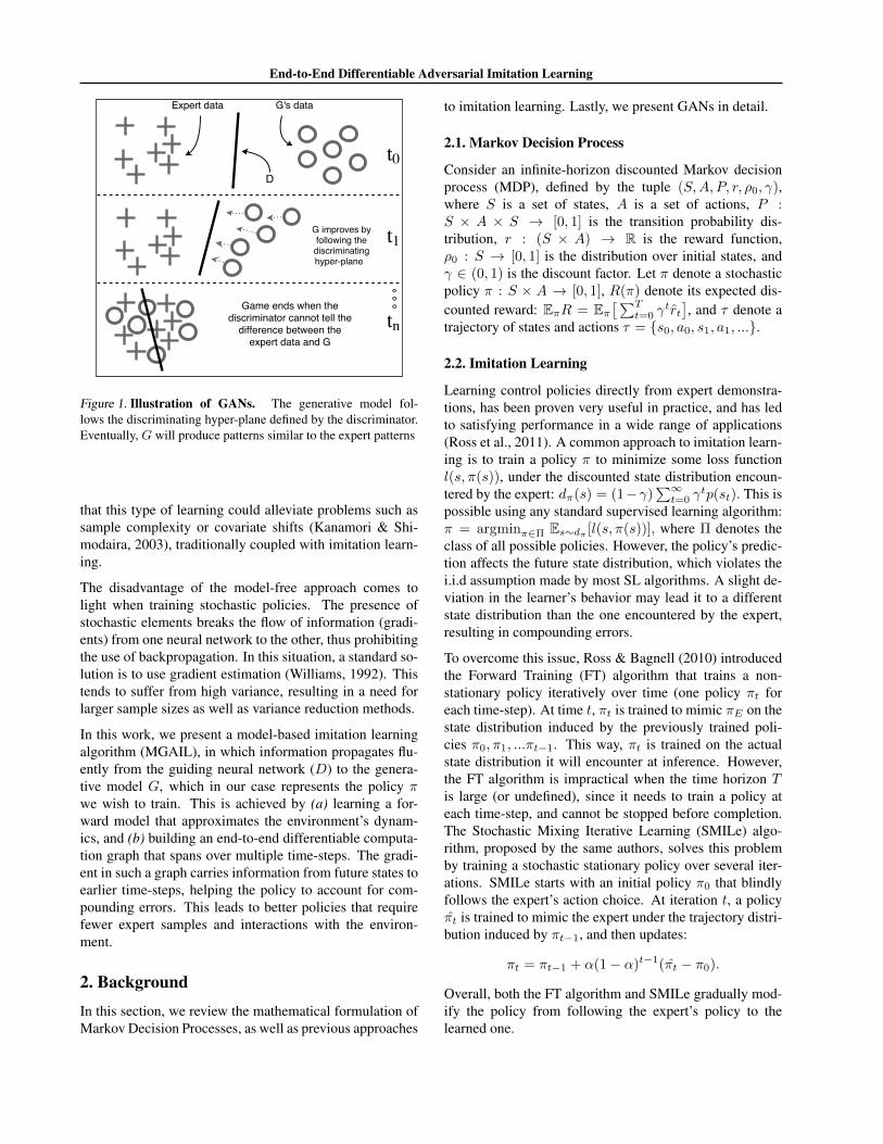
Figure 1. Illustration of GANs. The generative model fol-lows the discriminating hyper-plane defined by the discriminator.Eventually, G will produce patterns similar to the expert patterns

that this type of learning could alleviate problems such assample complexity or covariate shifts (Kanamori & Shi-modaira, 2003), traditionally coupled with imitation learn-ing.

The disadvantage of the model-free approach comes tolight when training stochastic policies. The presence ofstochastic elements breaks the flow of information (gradi-ents) from one neural network to the other, thus prohibitingthe use of backpropagation. In this situation, a standard so-lution is to use gradient estimation (Williams, 1992). Thistends to suffer from high variance, resulting in a need forlarger sample sizes as well as variance reduction methods.

In this work, we present a model-based imitation learningalgorithm (MGAIL), in which information propagates flu-ently from the guiding neural network (D) to the genera-tive model G, which in our case represents the policy πwe wish to train. This is achieved by (a) learning a for-ward model that approximates the environment’s dynam-ics, and (b) building an end-to-end differentiable computa-tion graph that spans over multiple time-steps. The gradi-ent in such a graph carries information from future states toearlier time-steps, helping the policy to account for com-pounding errors. This leads to better policies that requirefewer expert samples and interactions with the environ-ment.

2. BackgroundIn this section, we review the mathematical formulation ofMarkov Decision Processes, as well as previous approaches

to imitation learning. Lastly, we present GANs in detail.

2.1. Markov Decision Process

Consider an infinite-horizon discounted Markov decisionprocess (MDP), defined by the tuple (S,A, P, r, ρ0, γ),where S is a set of states, A is a set of actions, P :S × A × S → [0, 1] is the transition probability dis-tribution, r : (S × A) → R is the reward function,ρ0 : S → [0, 1] is the distribution over initial states, andγ ∈ (0, 1) is the discount factor. Let π denote a stochasticpolicy π : S × A → [0, 1], R(π) denote its expected dis-counted reward: EπR = Eπ

[∑Tt=0 γ

trt], and τ denote a

trajectory of states and actions τ = {s0, a0, s1, a1, ...}.

2.2. Imitation Learning

Learning control policies directly from expert demonstra-tions, has been proven very useful in practice, and has ledto satisfying performance in a wide range of applications(Ross et al., 2011). A common approach to imitation learn-ing is to train a policy π to minimize some loss functionl(s, π(s)), under the discounted state distribution encoun-tered by the expert: dπ(s) = (1−γ)

∑∞t=0 γ

tp(st). This ispossible using any standard supervised learning algorithm:π = argminπ∈Π Es∼dπ [l(s, π(s))], where Π denotes theclass of all possible policies. However, the policy’s predic-tion affects the future state distribution, which violates thei.i.d assumption made by most SL algorithms. A slight de-viation in the learner’s behavior may lead it to a differentstate distribution than the one encountered by the expert,resulting in compounding errors.

To overcome this issue, Ross & Bagnell (2010) introducedthe Forward Training (FT) algorithm that trains a non-stationary policy iteratively over time (one policy πt foreach time-step). At time t, πt is trained to mimic πE on thestate distribution induced by the previously trained poli-cies π0, π1, ...πt−1. This way, πt is trained on the actualstate distribution it will encounter at inference. However,the FT algorithm is impractical when the time horizon Tis large (or undefined), since it needs to train a policy ateach time-step, and cannot be stopped before completion.The Stochastic Mixing Iterative Learning (SMILe) algo-rithm, proposed by the same authors, solves this problemby training a stochastic stationary policy over several iter-ations. SMILe starts with an initial policy π0 that blindlyfollows the expert’s action choice. At iteration t, a policyπt is trained to mimic the expert under the trajectory distri-bution induced by πt−1, and then updates:

πt = πt−1 + α(1− α)t−1(πt − π0).

Overall, both the FT algorithm and SMILe gradually mod-ify the policy from following the expert’s policy to thelearned one.


2.3. Generative Adversarial Networks

GANs learn a generative model using a two-player zero-sum game:

argminG

argmaxD∈(0,1)

ExvpE [logD(x)]+

Ezvpz[

log(1−D(G(z))

)],

(2)

where pz is some noise distribution. In this game, player Gproduces patterns (denoted as x), and the second one (D)judges their authenticity. It does so by solving a binaryclassification problem where G’s patterns are labeled as 0,and expert patterns are labeled as 1. At the point whenD (the judge) can no longer discriminate between the twodistributions, the game ends since G has learned to mimicthe expert.

The two players are modeled by neural networks (with pa-rameters θd, θg respectively), therefore, their combinationcreates an end-to-end differentiable computation graph.For this reason, G can train by generating patterns, feed-ing it to D, and minimize the probability that D assigns tothem:

l(z, θg) = log(1−D(Gθg (z))

),

The benefit of GANs is that it relieves us from the need todefine a loss function or to handle complex models such asRBM’s and DBN’s (Lee et al., 2009). Instead, GANs relyon basic ideas (binary classification), and basic algorithms(backpropagation). The judge D trains to solve a binaryclassification problem by ascending at the following gradi-ent:

∇θd1

m

m∑i=1

[logDθd

(x(i))

+ log(

1−Dθd

(G(z(i)

))],

interchangeably while G descends at the following direc-tion:

∇θg1

m

m∑i=1

log(

1−D(Gθg (z(i))

)).

Ho & Ermon (2016) (GAIL) proposed to apply GANs toan expert policy imitation task in a model-free approach.GAIL draws a similar objective function like GANs, exceptthat here pE stands for the expert’s joint distribution overstate-action tuples:

argminπ

argmaxD∈(0,1)

Eπ[logD(s, a)]+

EπE [log(1−D(s, a))]− λH(π),(3)

where H(λ) , Eπ[− log π(a|s)] is the entropy.

The new game defined by Eq. 3 can no longer be solvedusing the standard tools mentioned above because playerG(i.e., the policy π) is now stochastic. Following this mod-ification, the exact form of the first term in Eq. 3 is given

by Es∼ρπ(s)Ea∼π(·|s)[logD(s, a)], instead of the followingexpression if π was deterministic: Es∼ρ[logD(s, π(s))].The resulting game depends on the stochastic properties ofthe policy. So, assuming that π = πθ, it is no longer clearhow to differentiate Eq. 3 w.r.t. θ. A standard solution isto use score function methods (Fu, 2006), of which RE-INFORCE is a special case (Williams, 1992), to obtain anunbiased gradient estimation:

∇θEπ[logD(s, a)] ∼= Eτi [∇θ log πθ(a|s)Q(s, a)], (4)

where Q(s, a) is the score function of the gradient:

Q(s, a) = Eτi [logD(s, a) | s0 = s, a0 = a]. (5)

Although unbiased, REINFORCE gradients tend to sufferhigh variance, which makes it hard to work with even afterapplying variance reduction techniques (Ranganath et al.,2014; Mnih & Gregor, 2014). In the case of GANs, the dif-ference between using the exact gradient and REINFORCEcan be explained in the following way: with REINFORCE,G asks D whether the pattern it generates are authentic ornot. D in return provides a brief Yes/No answer. On theother hand, using the exact gradient, G gets access to theinternal decision making logic of D. Thus it is better ableto understand the changes needed to foolD. Such informa-tion is present in the Jacobian of D.

In this work, we show how a forward model utilizes theJacobian of D when training π, without resorting to high-variance gradient estimations. The challenge of this ap-proach is that it requires learning a differentiable approx-imation to the environment’s dynamics. Errors in the for-ward model introduce a bias to the policy gradient whichimpairs the ability of π to learn robust and competent poli-cies. We share our insights regarding how to train forwardmodels, and in subsection 3.5 present an architecture thatwas found empirically adequate in modeling complex dy-namics.

3. AlgorithmWe start this section by analyzing the characteristics of thediscriminator. Then, we explain how a forward model canalleviate problems that arise when using GANs for policyimitation. Afterward, we present our model-based adver-sarial imitation algorithm. We conclude this section by pre-senting a forward model architecture that was found empir-ically adequate.

3.1. The discriminator network

The discriminator network is trained to predict the con-ditional distribution: D(s, a) = p(y|s, a) where y ∈{πE , π}. Put in words, D(s, a) represents the likelihoodratio that the pair {s, a} is generated by π rather than by


(a)

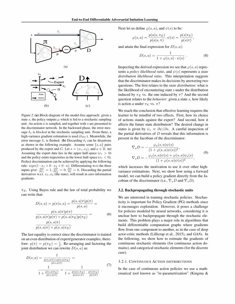
Figure 2. (a) Block-diagram of the model-free approach: given astate s, the policy outputs µ which is fed to a stochastic samplingunit. An action a is sampled, and together with s are presented tothe discriminator network. In the backward phase, the error mes-sage δa is blocked at the stochastic sampling unit. From there, ahigh-variance gradient estimation is used (δHV ). Meanwhile, theerror message δs is flushed. (b) Discarding δs can be disastrousas shown in the following example. Assume some {s, a} pairsproduced by the expert and G. Let s = (x1, x2), and a ∈ R. (c)Assuming the expert data lies in the upper half-space (x1 > 0)and the policy emits trajectories in the lower half-space (x1 < 0).Perfect discrimination can be achieved by applying the followingrule: sign(1 · x1 + 0 · x2 + 0 · a). Differentiating w.r.t the threeinputs give: ∂D

∂x1= 1, ∂D

∂x2= 0, ∂D

∂a= 0. Discarding the partial

derivatives w.r.t. x1, x2 (the state), will result in zero informationgradients.

πE . Using Bayes rule and the law of total probability wecan write that:

D(s, a) = p(π|s, a) =p(s, a|π)p(π)

p(s, a)=

p(s, a|π)p(π)

p(s, a|π)p(π) + p(s, a|πE)p(πE)=

p(s, a|π)

p(s, a|π) + p(s, a|πE).

(6)

The last equality is correct since the discriminator is trainedon an even distribution of expert/generator examples, there-fore: p(π) = p(πE) = 1

2 . Re-arranging and factoring thejoint distribution we can rewrite D(s, a) as:

D(s, a) =1

p(s,a|π)+p(s,a|πE)p(s,a|π)

=

1

1 + p(s,a|πE)p(s,a|π)

=1

1 + p(a|s,πE)p(a|s,π) ·

p(s|πE)p(s|π)

.

(7)

Next let us define ϕ(s, a), and ψ(s) to be:

ϕ(s, a) =p(a|s, πE)

p(a|s, π), ψ(s) =

p(s|πE)

p(s|π),

and attain the final expression for D(s, a):

D(s, a) =1

1 + ϕ(s, a) · ψ(s). (8)

Inspecting the derived expression we see that ϕ(s, a) repre-sents a policy likelihood ratio, and ψ(s) represents a statedistribution likelihood ratio. This interpretation suggeststhat the discriminator makes its decisions by answering twoquestions. The first relates to the state distribution: what isthe likelihood of encountering state s under the distributioninduced by πE vs. the one induced by π? And the secondquestion relates to the behavior: given a state s, how likelyis action a under πE vs. π?

We reach the conclusion that effective learning requires thelearner to be mindful of two effects. First, how its choiceof actions stands against the expert? And second, how itaffects the future state distribution? The desired change instates is given by ψs ≡ ∂ψ/∂s. A careful inspection ofthe partial derivatives of D reveals that this information ispresent in the Jacobian of the discriminator:

∇aD = − ϕa(s, a)ψ(s)

(1 + ϕ(s, a)ψ(s))2,

∇sD = −ϕs(s, a)ψ(s) + ϕ(s, a)ψs(s)

(1 + ϕ(s, a)ψ(s))2,

(9)

which increases the motivation to use it over other high-variance estimations. Next, we show how using a forwardmodel, we can build a policy gradient directly from the Ja-cobian of the discriminator (i.e.,∇aD and ∇sD).

3.2. Backpropagating through stochastic units

We are interested in training stochastic policies. Stochas-ticity is important for Policy Gradient (PG) methods sinceit encourages exploration. However, it poses a challengefor policies modeled by neural networks, considering it isunclear how to backpropagate through the stochastic ele-ments. This problem plays a major role in algorithms thatbuild differentiable computation graphs where gradientsflow from one component to another, as in the case of deepactor-critic methods (Lillicrap et al., 2015), and GANs. Inthe following, we show how to estimate the gradients ofcontinuous stochastic elements (for continuous action do-mains), and categorical stochastic elements (for the discretecase).

3.2.1. CONTINUOUS ACTION DISTRIBUTIONS

In the case of continuous action policies we use a math-ematical tool known as ”re-parametrization” (Kingma &


Welling, 2013; Rezende et al., 2014), which enables com-puting the derivatives of stochastic models. Assume astochastic policy with a Gaussian distribution1, where themean and variance are given by some deterministic func-tions µθ and σθ, respectively: πθ(a|s) ∼ N (µθ(s), σ

2θ(s)).

It is possible to re-write π as πθ(a|s) = µθ(s) + ξσθ(s),where ξ ∼ N (0, 1). In this way, we are able to get a Monte-Carlo estimator of the derivative of the expected value ofD(s, a) with respect to θ:

∇θEπ(a|s)D(s, a) =Eρ(ξ)∇aD(a, s)∇θπθ(a|s) ∼=

1

M

M∑i=1

∇aD(s, a)∇θπθ(a|s)∣∣∣ξ=ξi

.

(10)

3.2.2. CATEGORICAL ACTION DISTRIBUTIONS

For the case of discrete action domains, we suggest tofollow the idea of categorical re-parametrization withGumbel-Softmax (Maddison et al., 2016; Jang et al.,2016). This approach relies on the Gumbel-Max trick(Gumbel & Lieblein, 1954); a method to draw samplesfrom a categorical distribution with class probabilitiesπ(a1|s), π(a2|s), ...π(aN |s):

aargmax = argmaxi

[gi + log π(ai|s)],

where gi ∼ Gumbel(0, 1). Gumbel-Softmax provides adifferentiable approximation of the hard sampling proce-dure in the Gumbel-Max trick, by replacing the argmaxoperation with a softmax:

asoftmax =exp[

1τ (gi + log π(ai|s))

]∑kj=1 exp

[1τ (gj + log π(ai|s))

] ,where τ is a ”temperature” hyper-parameter that trades biaswith variance. When τ approaches zero, the softmax oper-ator acts like argmax (asoftmax ≈ aargmax) resulting in lowbias. However, the variance of the gradient ∇θasoftmax in-creases. Alternatively, when τ is set to a large value, thesoftmax operator creates a smoothing effect. This leadsto low variance gradients, but at the cost of a high bias(asoftmax 6= aargmax).

We use asoftmax, that is not necessarily ”one-hot”, to inter-act with the environment, which expects a single (”pure”)action. We solve this by applying argmax over asoftmax, butuse the continuous approximation in the backward passby using the estimation: ∇θaargmax ≈ ∇θasoftmax.

1A general version of the re-parametrization trick for otherdistributions such as beta or gamma was recently proposed byRuiz et al. (2016)

3.3. Backpropagating through a Forward model

So far we showed the changes necessary to use the exactpartial derivative ∇aD. Incorporating the use of ∇sD aswell is a more involved and constitutes the crux of thiswork. To understand why, we can look at the block dia-gram of the model-free approach in Figure 2. There, s istreated as fixed (it is given as an input), therefore ∇sD isdiscarded. On the contrary, in the model-based approach,st can be written as a function of the previous state and ac-tion: st = f(st−1, at−1), where f is the forward model.This way, using the law of total derivatives, we get that:

∇θD(st, at)

∣∣∣∣∣s=st,a=at

=∂D

∂a

∂a

∂θ

∣∣∣∣∣a=at

+∂D

∂s

∂s

∂θ

∣∣∣∣∣s=st

=

∂D

∂a

∂a

∂θ

∣∣∣∣∣a=at

+∂D

∂s

(∂f

∂s

∂s

∂θ

∣∣∣∣∣s=st−1

+∂f

∂a

∂a

∂θ

∣∣∣∣∣a=at−1

).

(11)

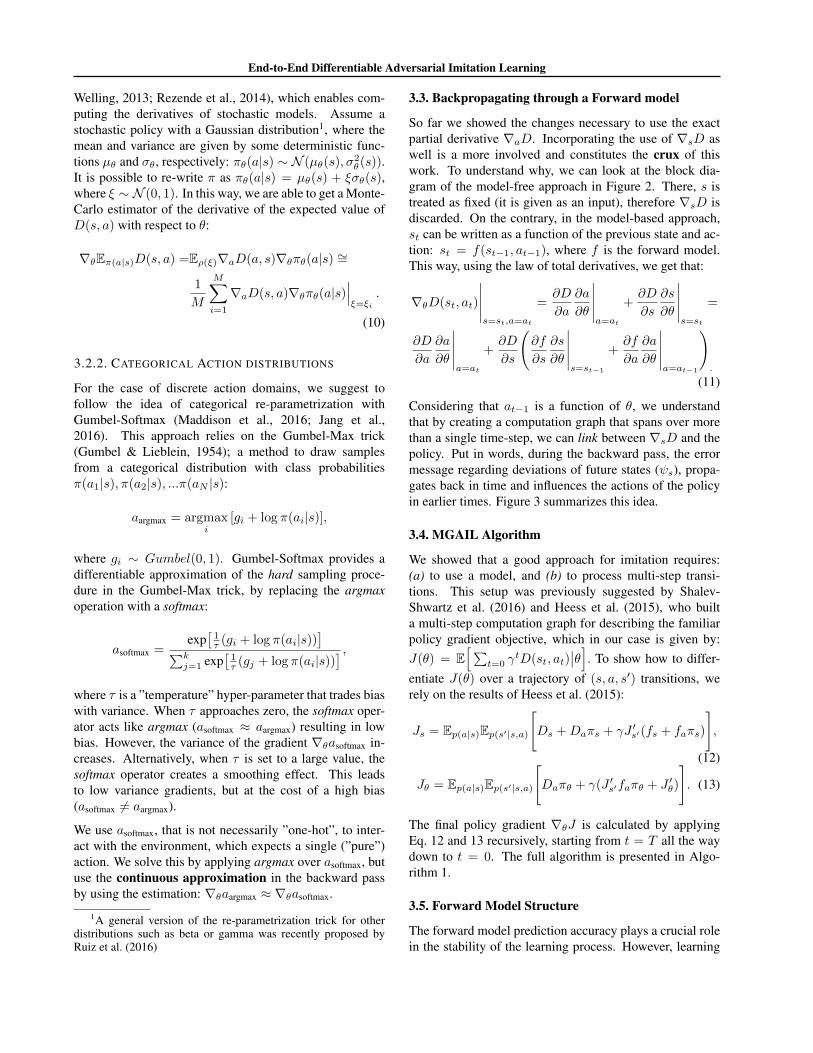
Considering that at−1 is a function of θ, we understandthat by creating a computation graph that spans over morethan a single time-step, we can link between ∇sD and thepolicy. Put in words, during the backward pass, the errormessage regarding deviations of future states (ψs), propa-gates back in time and influences the actions of the policyin earlier times. Figure 3 summarizes this idea.

3.4. MGAIL Algorithm

We showed that a good approach for imitation requires:(a) to use a model, and (b) to process multi-step transi-tions. This setup was previously suggested by Shalev-Shwartz et al. (2016) and Heess et al. (2015), who builta multi-step computation graph for describing the familiarpolicy gradient objective, which in our case is given by:J(θ) = E

[∑t=0 γ

tD(st, at)∣∣θ]. To show how to differ-

entiate J(θ) over a trajectory of (s, a, s′) transitions, werely on the results of Heess et al. (2015):

Js = Ep(a|s)Ep(s′|s,a)

[Ds +Daπs + γJ ′s′(fs + faπs)

],

(12)

Jθ = Ep(a|s)Ep(s′|s,a)

[Daπθ + γ(J ′s′faπθ + J ′θ)

]. (13)

The final policy gradient ∇θJ is calculated by applyingEq. 12 and 13 recursively, starting from t = T all the waydown to t = 0. The full algorithm is presented in Algo-rithm 1.

3.5. Forward Model Structure

The forward model prediction accuracy plays a crucial rolein the stability of the learning process. However, learning


Figure 3. Block diagram of model-based adversarial imitation learning. This diagram describes the computation graph for trainingthe policy (i.e. G). The discriminator network D is fixed at this stage and is trained separately. At time t of the forward pass, π outputsa distribution over actions: µt = π(st), from which an action at is sampled. For example, in the continuous case, this is done using there-parametrization trick: at = µt + ξ · σ, where ξ ∼ N (0, 1). The next state st+1 = f(st, at) is computed using the forward model(which is also trained separately), and the entire process repeats for time t+ 1. In the backward pass, the gradient of π is comprised ofa.) the error message δa (Green) that propagates fluently through the differentiable approximation of the sampling process. And b.) theerror message δs (Blue) of future time-steps, that propagate back through the differentiable forward model.

Algorithm 1 Model-based Generative Adversarial Imi-tation Learning

1: Input: Expert trajectories τE , experience buffer B, ini-tial policy and discriminator parameters θg , θd

2: for trajectory = 0 to∞ do3: for t = 0 to T do4: Act on environment: a = π(s, ξ; θg)5: Push (s, a, s′) into B6: end for7: train forward model f using B8: train discriminator model Dθd using B9: set: j′s = 0, j′θg = 0

10: for t = T down to 0 do11: jθg = [Daπθg + γ(j′s′faπθg + j′θg )]

∣∣ξ

12: js = [Ds +Daπs + γj′s′(fs + faπθg )]∣∣ξ

13: end for14: Apply gradient update using j0

θg15: end for

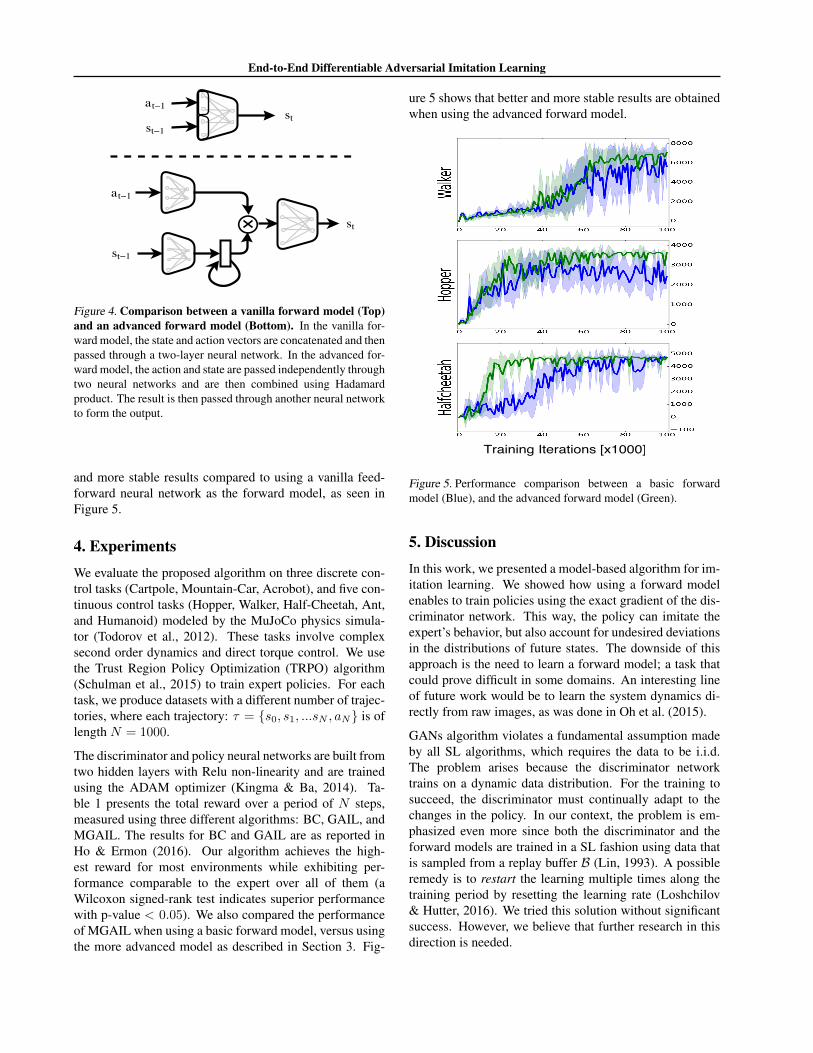
an accurate forward model is a challenging problem by it-self. We found that the performance of the forward modelcan be improved by considering the following two aspectsof its functionality. First, the forward model should learn touse the action as an operator over the state space. Actionsand states are sampled from entirely different distributions,so it would be preferable to first represent both in a sharedspace. Therefore, we first encode the state and action withtwo separate neural networks and then combine them toform a single vector. We found empirically that using aHadamard product to combine the encoded state and actionachieves the best performance. Additionally, predicting thenext state based on the current state alone requires the envi-ronment to be representable as a first order MDP. Instead,we can assume the environment to be representable as ann’th order MDP and use multiple previous states to pre-dict the next state. To model the multi-step dependencies,we use a recurrent connection from the previous state byincorporating a GRU layer (Cho et al., 2014) as part ofthe state encoder. Introducing these two modifications (seeFigure 4), we found the complete model to achieve better


Figure 4. Comparison between a vanilla forward model (Top)and an advanced forward model (Bottom). In the vanilla for-ward model, the state and action vectors are concatenated and thenpassed through a two-layer neural network. In the advanced for-ward model, the action and state are passed independently throughtwo neural networks and are then combined using Hadamardproduct. The result is then passed through another neural networkto form the output.

and more stable results compared to using a vanilla feed-forward neural network as the forward model, as seen inFigure 5.

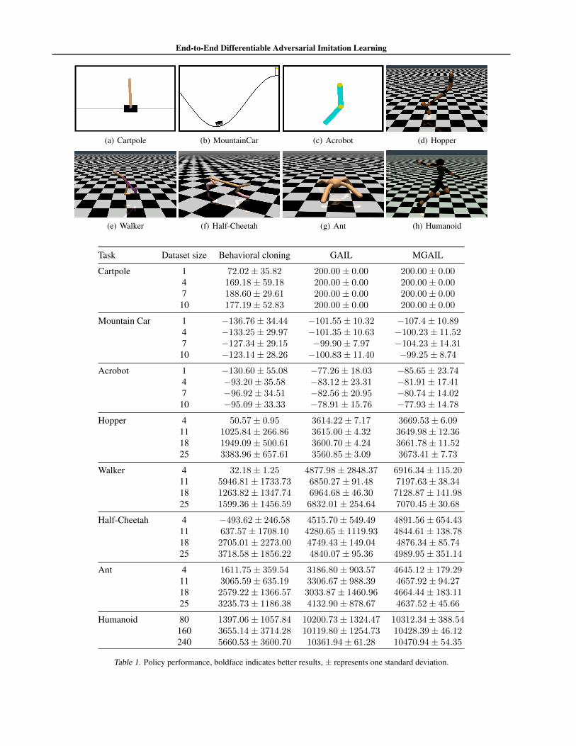
4. ExperimentsWe evaluate the proposed algorithm on three discrete con-trol tasks (Cartpole, Mountain-Car, Acrobot), and five con-tinuous control tasks (Hopper, Walker, Half-Cheetah, Ant,and Humanoid) modeled by the MuJoCo physics simula-tor (Todorov et al., 2012). These tasks involve complexsecond order dynamics and direct torque control. We usethe Trust Region Policy Optimization (TRPO) algorithm(Schulman et al., 2015) to train expert policies. For eachtask, we produce datasets with a different number of trajec-tories, where each trajectory: τ = {s0, s1, ...sN , aN} is oflength N = 1000.

The discriminator and policy neural networks are built fromtwo hidden layers with Relu non-linearity and are trainedusing the ADAM optimizer (Kingma & Ba, 2014). Ta-ble 1 presents the total reward over a period of N steps,measured using three different algorithms: BC, GAIL, andMGAIL. The results for BC and GAIL are as reported inHo & Ermon (2016). Our algorithm achieves the high-est reward for most environments while exhibiting per-formance comparable to the expert over all of them (aWilcoxon signed-rank test indicates superior performancewith p-value < 0.05). We also compared the performanceof MGAIL when using a basic forward model, versus usingthe more advanced model as described in Section 3. Fig-

ure 5 shows that better and more stable results are obtainedwhen using the advanced forward model.

Figure 5. Performance comparison between a basic forwardmodel (Blue), and the advanced forward model (Green).

5. DiscussionIn this work, we presented a model-based algorithm for im-itation learning. We showed how using a forward modelenables to train policies using the exact gradient of the dis-criminator network. This way, the policy can imitate theexpert’s behavior, but also account for undesired deviationsin the distributions of future states. The downside of thisapproach is the need to learn a forward model; a task thatcould prove difficult in some domains. An interesting lineof future work would be to learn the system dynamics di-rectly from raw images, as was done in Oh et al. (2015).

GANs algorithm violates a fundamental assumption madeby all SL algorithms, which requires the data to be i.i.d.The problem arises because the discriminator networktrains on a dynamic data distribution. For the training tosucceed, the discriminator must continually adapt to thechanges in the policy. In our context, the problem is em-phasized even more since both the discriminator and theforward models are trained in a SL fashion using data thatis sampled from a replay buffer B (Lin, 1993). A possibleremedy is to restart the learning multiple times along thetraining period by resetting the learning rate (Loshchilov& Hutter, 2016). We tried this solution without significantsuccess. However, we believe that further research in thisdirection is needed.


(a) Cartpole (b) MountainCar (c) Acrobot (d) Hopper

(e) Walker (f) Half-Cheetah (g) Ant (h) Humanoid

Task Dataset size Behavioral cloning GAIL MGAIL

Cartpole 1 72.02± 35.82 200.00± 0.00 200.00± 0.004 169.18± 59.18 200.00± 0.00 200.00± 0.007 188.60± 29.61 200.00± 0.00 200.00± 0.0010 177.19± 52.83 200.00± 0.00 200.00± 0.00

Mountain Car 1 −136.76± 34.44 −101.55± 10.32 −107.4± 10.894 −133.25± 29.97 −101.35± 10.63 −100.23± 11.527 −127.34± 29.15 −99.90± 7.97 −104.23± 14.3110 −123.14± 28.26 −100.83± 11.40 −99.25± 8.74

Acrobot 1 −130.60± 55.08 −77.26± 18.03 −85.65± 23.744 −93.20± 35.58 −83.12± 23.31 −81.91± 17.417 −96.92± 34.51 −82.56± 20.95 −80.74± 14.0210 −95.09± 33.33 −78.91± 15.76 −77.93± 14.78

Hopper 4 50.57± 0.95 3614.22± 7.17 3669.53± 6.0911 1025.84± 266.86 3615.00± 4.32 3649.98± 12.3618 1949.09± 500.61 3600.70± 4.24 3661.78± 11.5225 3383.96± 657.61 3560.85± 3.09 3673.41± 7.73

Walker 4 32.18± 1.25 4877.98± 2848.37 6916.34± 115.2011 5946.81± 1733.73 6850.27± 91.48 7197.63± 38.3418 1263.82± 1347.74 6964.68± 46.30 7128.87± 141.9825 1599.36± 1456.59 6832.01± 254.64 7070.45± 30.68

Half-Cheetah 4 −493.62± 246.58 4515.70± 549.49 4891.56± 654.4311 637.57± 1708.10 4280.65± 1119.93 4844.61± 138.7818 2705.01± 2273.00 4749.43± 149.04 4876.34± 85.7425 3718.58± 1856.22 4840.07± 95.36 4989.95± 351.14

Ant 4 1611.75± 359.54 3186.80± 903.57 4645.12± 179.2911 3065.59± 635.19 3306.67± 988.39 4657.92± 94.2718 2579.22± 1366.57 3033.87± 1460.96 4664.44± 183.1125 3235.73± 1186.38 4132.90± 878.67 4637.52± 45.66

Humanoid 80 1397.06± 1057.84 10200.73± 1324.47 10312.34± 388.54160 3655.14± 3714.28 10119.80± 1254.73 10428.39± 46.12240 5660.53± 3600.70 10361.94± 61.28 10470.94± 54.35

Table 1. Policy performance, boldface indicates better results, ± represents one standard deviation.


This research was supported in part by the European Com-munitys Seventh Framework Programme (FP7/2007-2013)under grant agreement 306638 (SUPREL) and the IntelCollaborative Research Institute for Computational Intel-ligence (ICRI-CI).

ReferencesCho, Kyunghyun, van Merrienboer, Bart, Gulcehre, Caglar,

Bougares, Fethi, Schwenk, Holger, and Bengio, Yoshua.Learning phrase representations using RNN encoder-decoderfor statistical machine translation. CoRR, abs/1406.1078,2014.

Dorigo, Marco and Colombetti, Marco. Robot shaping: an exper-iment in behavior engineering. MIT press, 1998.

Fu, Michael C. Gradient estimation. Handbooks in operationsresearch and management science, 13:575–616, 2006.

Goodfellow, Ian, Pouget-Abadie, Jean, Mirza, Mehdi, Xu, Bing,Warde-Farley, David, Ozair, Sherjil, Courville, Aaron, andBengio, Yoshua. Generative adversarial nets. In Advances inNeural Information Processing Systems, pp. 2672–2680, 2014.

Gumbel, Emil Julius and Lieblein, Julius. Statistical theory ofextreme values and some practical applications: a series of lec-tures. 1954.

Heess, Nicolas, Wayne, Gregory, Silver, David, Lillicrap, Tim,Erez, Tom, and Tassa, Yuval. Learning continuous control poli-cies by stochastic value gradients. In Advances in Neural In-formation Processing Systems, pp. 2944–2952, 2015.

Ho, Jonathan and Ermon, Stefano. Generative adversarial imita-tion learning. arXiv preprint arXiv:1606.03476, 2016.

Jang, Eric, Gu, Shixiang, and Poole, Ben. Categoricalreparameterization with gumbel-softmax. arXiv preprintarXiv:1611.01144, 2016.

Kanamori, Takafumi and Shimodaira, Hidetoshi. Active learn-ing algorithm using the maximum weighted log-likelihood es-timator. Journal of statistical planning and inference, 116(1):149–162, 2003.

Kingma, Diederik and Ba, Jimmy. Adam: A method for stochas-tic optimization. arXiv preprint arXiv:1412.6980, 2014.

Kingma, Diederik P and Welling, Max. Auto-encoding variationalbayes. arXiv preprint arXiv:1312.6114, 2013.

Lee, Honglak, Grosse, Roger, Ranganath, Rajesh, and Ng, An-drew Y. Convolutional deep belief networks for scalable unsu-pervised learning of hierarchical representations. In Proceed-ings of the 26th annual international conference on machinelearning, pp. 609–616. ACM, 2009.

Lillicrap, Timothy P, Hunt, Jonathan J, Pritzel, Alexander, Heess,Nicolas, Erez, Tom, Tassa, Yuval, Silver, David, and Wierstra,Daan. Continuous control with deep reinforcement learning.arXiv preprint arXiv:1509.02971, 2015.

Lin, Long-Ji. Reinforcement learning for robots using neural net-works. Technical report, DTIC Document, 1993.

Loshchilov, Ilya and Hutter, Frank. Sgdr: Stochastic gradientdescent with restarts. arXiv preprint arXiv:1608.03983, 2016.

Maddison, Chris J, Mnih, Andriy, and Teh, Yee Whye. The con-crete distribution: A continuous relaxation of discrete randomvariables. arXiv preprint arXiv:1611.00712, 2016.

Mathieu, Michael, Couprie, Camille, and LeCun, Yann. Deepmulti-scale video prediction beyond mean square error. arXivpreprint arXiv:1511.05440, 2015.

Mirza, Mehdi and Osindero, Simon. Conditional generative ad-versarial nets. arXiv preprint arXiv:1411.1784, 2014.

Mnih, Andriy and Gregor, Karol. Neural variational inference andlearning in belief networks. arXiv preprint arXiv:1402.0030,2014.

Ng, Andrew Y, Russell, Stuart J, et al. Algorithms for inversereinforcement learning. In Icml, pp. 663–670, 2000.

Oh, Junhyuk, Guo, Xiaoxiao, Lee, Honglak, Lewis, Richard L,and Singh, Satinder. Action-conditional video prediction usingdeep networks in atari games. In Advances in Neural Informa-tion Processing Systems, pp. 2863–2871, 2015.

Pomerleau, Dean A. Efficient training of artificial neural networksfor autonomous navigation. Neural Computation, 3(1):88–97,1991.

Ranganath, Rajesh, Gerrish, Sean, and Blei, David M. Black boxvariational inference. In AISTATS, pp. 814–822, 2014.

Rezende, Danilo Jimenez, Mohamed, Shakir, and Wierstra, Daan.Stochastic backpropagation and approximate inference in deepgenerative models. arXiv preprint arXiv:1401.4082, 2014.

Ross, Stephane and Bagnell, Drew. Efficient reductions for imi-tation learning. In AISTATS, pp. 661–668, 2010.

Ross, Stephane, Gordon, Geoffrey J, and Bagnell, Drew. A reduc-tion of imitation learning and structured prediction to no-regretonline learning. In AISTATS, volume 1, pp. 6, 2011.

Ruiz, Francisco R, AUEB, Michalis Titsias RC, and Blei, David.The generalized reparameterization gradient. In Advances inNeural Information Processing Systems, pp. 460–468, 2016.


Rusu, Andrei A, Colmenarejo, Sergio Gomez, Gulcehre, Caglar,Desjardins, Guillaume, Kirkpatrick, James, Pascanu, Razvan,Mnih, Volodymyr, Kavukcuoglu, Koray, and Hadsell, Raia.Policy distillation. arXiv preprint arXiv:1511.06295, 2015.

Schulman, John, Levine, Sergey, Moritz, Philipp, Jordan,Michael I, and Abbeel, Pieter. Trust region policy optimiza-tion. CoRR, abs/1502.05477, 2015.

Shalev-Shwartz, Shai, Ben-Zrihem, Nir, Cohen, Aviad, andShashua, Amnon. Long-term planning by short-term predic-tion. arXiv preprint arXiv:1602.01580, 2016.

Sutton, Richard S. Learning to predict by the methods of temporaldifferences. Machine learning, 3(1):9–44, 1988.

Sutton, Richard Stuart. Temporal credit assignment in reinforce-ment learning. 1984.

Todorov, Emanuel, Erez, Tom, and Tassa, Yuval. Mujoco: Aphysics engine for model-based control. In Intelligent Robotsand Systems (IROS), 2012 IEEE/RSJ International Conferenceon, pp. 5026–5033. IEEE, 2012.

Williams, Ronald J. Simple statistical gradient-following al-gorithms for connectionist reinforcement learning. Machinelearning, 8(3-4):229–256, 1992.

Ziebart, Brian D, Maas, Andrew L, Bagnell, J Andrew, and Dey,Anind K. Maximum entropy inverse reinforcement learning.In AAAI, pp. 1433–1438, 2008.

Documents

End-to-End Differentiable Adversarial Imitation Learningproceedings.mlr.press/v70/baram17a/baram17a.pdf · End-to-End Differentiable Adversarial Imitation Learning 2.3. Generative