Annu. Rev. Neurosci. 2003. 26:X--Xdoi: 10.1146/annurev.neuro.26.041002.131112

Copyright © 2003 by Annual Reviews. All rights reserved<DOI>10.1146/annurev.neuro.26.041002.131112</DOI>0147-006X/03/0721-0000$14.00POUGET  DAYAN  ZEMEL

[AU: PLEASE CHOOSE A RUNNING HEAD FEWER THAN 38 CHARACTERS AND SPACES

CODING AND COMPUTATION]POPULATION CODING AND COMPUTATION]

INFERENCE AND COMPUTATION WITH POPULATION CODES

A. Pouget,1 P. Dayan,2 R.S. Zemel3[AU: is this how you want your names in the book

and on the front cover? YES]1 Department of Brain and Cognitive Sciences, Meliora Hall, University of Rochester,

Rochester, New York, 14627; email: alex@bcs.rochester.edu;2 Gatsby Computational Neuroscience Unit, Alexandra House, 17 Queen Square,

London WC1N 3AR, United Kingdom; email: dayan@gatsby.ucl.ac.uk;3Department of Computer Science, University of Toronto, Toronto, Ontario M5S 1A4

Canada; email: zemel@cs.toronto.edu

Key Words Firing rate, noise, decoding, Bayes rule, basis functions, probability

distribution, probabilistic inference

 Abstract [AU: Please write a 100-150-word abstract.]

In the vertebrate nervous system, sensory stimuli are typically encoded through the concerted activity of large populations of neurons. Classically, these patterns of activity have been treated as encoding the value of the stimulus (e.g. the orientation of a contour) and computation has been formalized in terms of function approximation. More recently, there have been several suggestions that neural computation is akin to a Bayesian inference process, with population activity patterns representing uncertainty about stimuli in the form of probability distributions (e.g. the probability density function over the orientation of a contour). This paper reviews both approaches, with a particular emphasis on the latter, which we see as a very promising framework for future modeling and experimental work.

INTRODUCTION

The way that neural activity represents sensory and motor information has been the

subject of intense investigation. A salient finding is that single aspects of the world (i.e.,

single variables) induce activity in multiple neurons. For instance, the direction of an air

current caused by movement of a nearby predator of a cricket is encoded in the concerted

1

activity of several neurons, called cercal interneurons (Theunissen & Miller 1991).

Further, each neuron is activated to a greater or lesser degree by different wind directions.

Evidence exists for this form of coding at the sensory input areas of the brain (e.g.,

retinotopic and tonotopic maps), as well as at the motor output level, and in many other

intermediate neural processing areas, including superior colliculus neurons encoding

saccade direction (Lee et al. 1988), MT[AU: please spell out on first instance Mmiddle

temporal] :Mmiddle temporal]cells responding to local velocity (Maunsell & Van Essen

1983), MST[AU: please spell out on first instance: mimiddle ssuperior ttemporal] : cells

sensitive to global motion parameters (Graziano et al. 1994), inferotemporal (IT) neurons

responding to human faces (Perrett et al. 1985), hippocampal place cells responding to

the location of a rat in an environment (O'Keefe & Dostrovsky 1971), and cells in

primary motor cortex of a monkey responding to the direction it is to move its arm

(Georgopoulos et al. 1982).

A major focus of theoretical neuroscience has been to understanding how populations

of neurons encode information about single variables; how this information can be

decoded from the population activity; how population codes support nonlinear

computations over the information they represent; how populations may offer a rich

representation of such things as uncertainty in the aspects of the stimuli they represent;

how multiple aspects of the world are represented in single populations; and what

computational advantages (or disadvantages) such schemes have. [AU: AR house style

does not use italics for emphasis or key words.]

Section 1The first section below, entitled The Standard Model, of this review considers

the standard model of population coding that is now part of the accepted canon of

systems neuroscience. Section 2The second section following, entitled Encoding

Probability Distributions, considers more recent proposals that extend the scope of the

standard model.

1  THE STANDARD MODEL

1.1 Coding and Decoding 

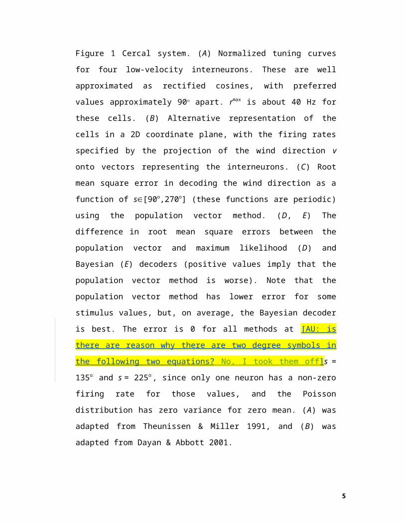
Figure 1A shows the normalized mean firing rates of the four low-velocity interneurons

of the cricket cercal system as a function of a stimulus variable s, which is the direction

2

of an air current that could have been induced by the movement of a nearby predator

(Theunissen & Miller 1991). This firing is induced by the activity of the primary sensory

neurons for the system, the hair cells on the cerci.

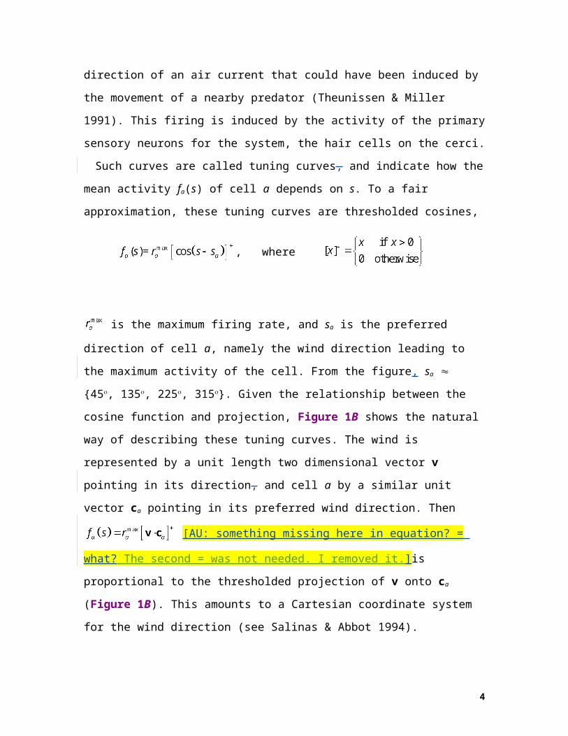
Such curves are called tuning curves, and indicate how the mean activity fa(s) of cell a

depends on s. To a fair approximation, these tuning curves are thresholded cosines,

, where

is the maximum firing rate, and sa is the preferred direction of cell a, namely the

wind direction leading to the maximum activity of the cell. From the figure, sa {45,

135, 225, 315}. Given the relationship between the cosine function and projection,

Figure 1B shows the natural way of describing these tuning curves. The wind is

represented by a unit length two dimensional vector v pointing in its direction, and cell a

by a similar unit vector ca pointing in its preferred wind direction. Then

[AU: something missing here in equation? = what? The second =

was not needed. I removed it.]is proportional to the thresholded projection of v onto ca

(Figure 1B). This amounts to a Cartesian coordinate system for the wind direction (see

Salinas & Abbot 1994).

Figure 1 Cercal system. (A) Normalized tuning curves for four low-velocity

interneurons. These are well approximated as rectified cosines, with preferred

values approximately 90 apart. rmax is about 40 Hz for these cells. (B) Alternative

representation of the cells in a 2D coordinate plane, with the firing rates specified

by the projection of the wind direction v onto vectors representing the

interneurons. (C) Root mean square error in decoding the wind direction as a

function of s[90o,270o] (these functions are periodic) using the population

vector method. (D, E) The difference in root mean square errors between the

population vector and maximum likelihood (D) and Bayesian (E) decoders

(positive values imply that the population vector method is worse). Note that the

population vector method has lower error for some stimulus values, but, on

average, the Bayesian decoder is best. The error is 0 for all methods at [AU: is

3

there are reason why there are two degree symbols in the following two

equations? No, I took them off]s = 135o and s = 225o, since only one neuron has

a non-zero firing rate for those values, and the Poisson distribution has zero

variance for zero mean. (A) was adapted from Theunissen & Miller 1991, and (B)

was adapted from Dayan & Abbott 2001.

The Cartesian population code uses just four preferred values; an alternative,

homogeneous form of coding allocates the neurons more evenly over the range of

variable values. One example of this is the representation of orientation in striate cortex

(Hubel & Wiesel 1962). Figure 2A (see color insert) shows an (invented) example of the

tuning curves of a population of orientation-tuned cells in V1 in response to small bars of

light of different orientations, presented at the best position on the retina. These can be

roughly characterized as Gaussians (or, more generally, bell-shaped curves), with a

standard deviation of = 15o. The highlighted cell has preferred orientation s = 180o,;

and preferred values are spread evenly across the circle. As we shall see, homogeneous

population codes are important because they provide the substrate for a wide range of

nonlinear computations.

For either population code, the actual activity on any particular occasion, for instance

the firing rate ra = na/t computed as the number of spikes na fired in a short time window

t, is not exactly fa(s), because neural activity is almost invariably noisy. Rather, it is a

random quantity (called a random variable) with mean ra = fa(s) (using to indicate

averaging over the randomness). We mostly consider the simplest reasonable model of

this for which the number of spikes na has a Poisson distribution. For this distribution, the

variance is equal to the mean, and there are no correlations in the noise that corrupting s

s[AU: ok? ‘no correlations that corrupt’. Or do you mean ‘in the noise that corrupts’? Is

the subject of ‘corrupt’ ‘correlations’ or ‘noise’? ‘noise’ is the subject in this case] the

activity of each member of the setpopulation of neurons contains no correlations (this is

indeed a good fair approximation to the noise found in the nervous system;, see, for

instance, Gershon et al. 1998, Shadlen et al. 1996, Tolhurst et al. 1982). In this review,

we also restrict our discussion to rate-based descriptions, ignoring the details of precise

spike -timing.

4

Equation 1, coupled with the Poisson assumption, is called an encoding model for the

wind direction s. One natural question, that we cannot yet answer, is how the activities of

the myriad hair cells actually give rise to such simple tuning. A more immediately

tractable question is how the wind direction s can be read out of, i.e., decoded, from the

noisy rates r. Decoding can be used as a computational tool, for instance, to assess the

fidelity with which the population manages to code for the stimulus, or (at least a lower

bound to) the information contained in the activities (Borst & Theunissen 1999, Rieke et

al. 1999). However, decoding is not an essential neurobiological operation, asbecause

there is almost never a reason to decode the stimulus explicitly. Rather, the population

code is used to support computations involving s, whose outputs are represented in the

form of yet more population codes over the same or different collections of neurons.

WeThe reader will see some Some examples of this will shortly be presented; for the

moment we consider the narrower, but still important, computational question of

extracting approximations to s.

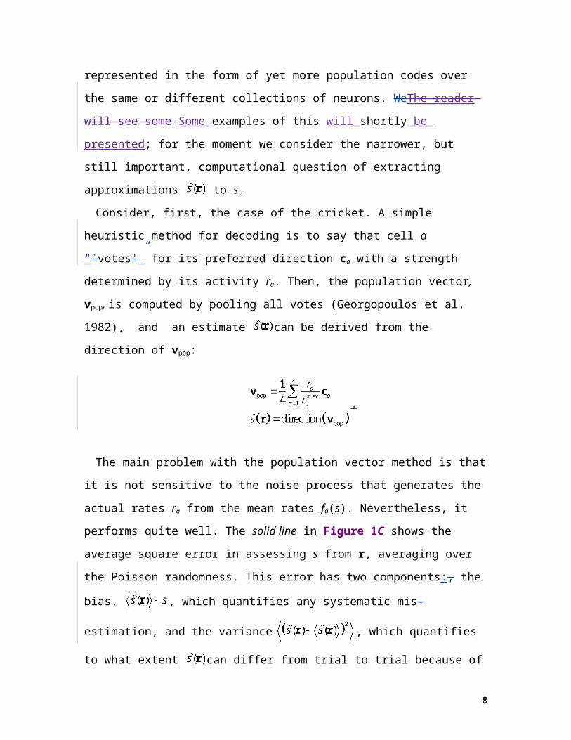
Consider, first, the case of the cricket. A simple heuristic method for decoding is to say

that cell a “`votes'” for its preferred direction ca with a strength determined by its activity

ra. Then, the population vector, vpop, is computed by pooling all votes (Georgopoulos et

al. 1982), and an estimate can be derived from the direction of vpop:

.

The main problem with the population vector method is that it is not sensitive to the

noise process that generates the actual rates ra from the mean rates fa(s). Nevertheless, it

performs quite well. The solid line in Figure 1C shows the average square error in

assessing s from r, averaging over the Poisson randomness. This error has two

components:, the bias, , which quantifies any systematic mis-estimation, and

the variance , which quantifies to what extent can differ from trial

to trial because of the random activities. In this case, the bias is small, but the variance is

5

appreciable. Nevertheless, with just 4 noisy neurons, estimation of wind direction to

within a few degrees is possible.

In order tTo evaluate the quality of the population vector method, we need to know the

fidelity with which better decoding methods can extract s from r. A particularly

important result from classical statistics is the Cramér-Rao lower bound (Papoulis 1991),

which provides a minimum value for the variance of any estimator as a function of

two quantities: the bias of the estimator, and an estimator-independent quantity called the

Fisher information IF for the population code, which is a measure of how different the

recorded activities are likely to be when two slightly different stimuli are presented. The

greater is the Fisher information, is, the smaller is the minimum variance is, and the better

is the potential quality of any estimator is (Paradiso 1988, Seung & Sompolinsky 1993).

The Fisher information is interestingly related to the Shannon information (s;r), which

quantifies the deviation from independence of the stimulus s and the noisy activities r

(see Brunel & Nadal 1998).

A particularly important estimator that in some limiting circumstances achieves the

Cramér-Rao lower bound is the maximum likelihood estimator (Papoulis 1991). This

estimator starts from the full probabilistic encoding model, which, by taking into account

the noise corrupting the activities of the neurons, specifies the probability P[r|s] of

observing activities r if the stimulus is s. For the Poisson encoding model, this is the so-

called likelihood :

.

Values of s for which P[r| s] is high are directions which that are likely to have produced

the observed activities r; values of s for which P[r|s] is low are unlikely. The maximum

likelihood estimate is the value that maximizes P[r|s]. Figure 1D shows, as a

function of s, how much better or worse the maximum likelihood estimator is than the

population vector. By taking correct account of the noise, it does a little better on

average.

When its estimates are based on the activity of many neurons (as is the case in an

homogeneous code), (Figure 2A), the maximum likelihood estimator can be shown to

6

possess many properties, such as being unbiased (Paradiso 1988, Seung & Sompolinsky

1993). Although the cercal system, and indeed most other invertebrate population codes,

involves only a few cells, most mammalian cortical population codes are homogeneous

and involve sufficient neurons for this theory to apply.

The final class of estimators, called Bayesian estimators, combine the likelihood P[r|s]

(Equation 2) with any prior information about the stimulus s (for instance, that some

wind directions are intrinsically more likely than others for predators) to produce a

posterior distribution P[sr] (Foldiak 1993, Sanger 1996):

.

When the prior distribution P[s] is a flat, that is when there is no specific prior

information about s, this is a renormalized version of the likelihood, where the

renormalization ensures that it is a proper probability distribution (i.e., integrates to 1).

The posterior distribution summarizes everything that the neural activity and any prior

information have to say about s, and so is the most complete basis for decoding. Bayesian

inference proceeds using a loss function L(s,s), which indicates the cost of reporting s

when the true value is s; it is optimal to decode to the value , thatwhich minimizes

the cost, averaged over the posterior distribution (DeGroot 1970). Figure 1E shows the

comparative quality of the Bayesian estimator. By including information from the whole

likelihood, and not just its peak, the Bayesian estimator does a little better than the

maximum likelihood and population vector methods. However, all methods work well

here.

Exactly the same set of methods applies to decoding homogeneous population codes as

Cartesian ones, with the Bayesian and maximum likelihood decoding typically

outperforming the population vector approach by a rather larger margin. In fact, some

calculations are easier, because the mean sum activity across the whole population is the

same whatever the value of the stimulus s. Also, in general, the greater is the number of

cells is, the greater is the accuracy with which the stimulus can be decoded by any

method, since more cells can provide more information about s. However, this conclusion

does depend on the way, if at all, that the noise corrupting the activity is correlated

7

between the cells (Abbott & Dayan 1999, Oram et al. 1998, Snippe & Koenderink 1992b,

Sompolinsky et al. 2001, Wilke & Eurich 2002, Yoon & Sompolinsky 1999), and the

way that information about these correlations is used by the decoders.

The reader should Nnote the relationship between Tthe Bayesian estimator and the

population vector method bear a subtle relationship to each other. In this simple case, the

former averages possible stimulus values s weighted by their (renormalized) likelihoods

P[r|s], rather than averaging preferred stimulus values ca weighted by the spike rates ra.

1.2 Computation with Population Codes

1.2.1 DISCRIMINATION One important computation based on population codes

involves using the spiking rates of the cells r to discriminate between different stimuli,

for instance, telling between orientations s* + s and s* s, where s is a small angle. It

is formally possible to perform discrimination by first decoding, say finding the Bayesian

posterior P[s|r], and then reporting whether it is more likely that s < s* or s > s*.

However, assuming the prior distribution does not favor either outcome, it is also

possible to perform discrimination based directly on the activities by computing a linear,

feedforward, test:

+ ,

where is usually 0 for a homogeneous population code, and wa = fa(s)/fa(s) (Figure.

2B). The appropriate report is s* + s if t(r) > 0 and s* s if t(r) < 0 (Pouget & Thorpe

1991, Seung & Sompolinsky 1993, Snippe & Koenderink 1992a). Figure 2B shows the

discrimination weights for the case that s* = 210o. The weight wa for cell a is proportional

to the slope of the tuning curve, fa(s), because the slope determines the amount by which

the mean activity of neuron a varies when the stimulus changes from s* - s to s* s:

the larger is the activity change is, the more informative the neuron is about the change in

the stimulus, and the larger is its weight is. Note an interesting consequence of this

principle: tThe neuron whose preferred value is actually the value about which the task is

set (sa = s*) has a weight of 0. This finding isoccurs because its slope is zero for s*, i.e.,

its mean activity is the same for s* + s and s* s, and so it is unhelpful for performing

the discrimination. The weight wa is also inversely proportional to the variance of the

8

activity of cell a, which is the same as the mean, fa(s). Psychophysical and

neurophysiological data indicate that this pattern of weights is indeed used in humans and

animals alike when performing fine discrimination (Hol & Treue 2001, Regan &

Beverley 1985).

Signal detection theory (Green & Swets 1966) underpins the use of population codes

for discrimination. Signal detection’s standard measure of discriminability, called d, is a

function of the Fisher information---, the same quantity that determines the quality of the

population code for decoding.

1.2.2 NOISE REMOVAL As discussed above, although the maximum likelihood

estimator is mathematically attractive, its neurobiological relevance is unclear. First,

finding a single scalar value seems unreasonable, sincebecause population codes seem to

be used almost throughout the brain. Second, in general, finding the maximum likelihood

value requires a solving a non-quadratic optimization problem (Bishop 1995).

Both of these problems can be addressed by utilizing recurrent connections within the

population to make it behave like an auto-associative memory (Hopfield 1982). Auto-

associative memories use nonlinear recurrent interactions to find the stored pattern that

most closely matches a noisy input. One can roughly characterize these devices in the

physical terms of a mountainous landscape. The pattern of neural activities at any time

(characterized by the firing rates of the neurons) is represented by a point on the surface.

The recurrent interactions have the effect of moving the point downhill (Cohen &

Grossberg 1983), and the stored memories induce dips or wells. In this case, a noisy

version of one of the inputs lies at a point displaced from the bottom of a well; the

nonlinear recurrent interactions move the state to the bottom of the closest well, and thus

perform retrieval. The bottoms of the wells are stable points for the recurrent dynamics.

Ben-Yishai et al. (1995),; Zhang (1996), and Seung (1996) constructed auto-

associative devices (called continuous, line or surface attractor networks) whose

landscapes have the structure of perfectly flat and one-dimensional (or perhaps higher-

dimensional) valleys. Points at the bottom of a valley represent perfectly smooth bell-

shaped activity profiles in the network. There is one point for each possible location s of

the peak (e.g., each possible orientation), with activities ra = fa(s). In this case, starting

from a noisy initial pattern r, the recurrent dynamics finds a point at the bottom of the

9

valley, and thus takes r into a perfectly smooth bell-shaped activity pattern fa(ŝ(r))

(Figure 3A, see color insert). This is how the scheme answers the first objection to

decoding: Iit does not directly find a scalar value, but instead integrates all the

information in the input and provides the answer in the form of another, but more perfect,

population code. Note that such recurrent networks are themselves used to model

activity-based short -term or working memory (Compte et al. 2000).

Pouget et al. (19989, Deneve, Latham Pouget19998) proved that a wide variety of

recurrent networks with continuous attractors can implement a close approximation to

maximum likelihood decoding, i.e., turning r into activities , with the smooth

bump centered at the maximum likelihood value. This result holds regardless of the

activation functions of the units (which determine how the input to a unit determines its

output firing rate), and includes networks that use biologically inspired activation

functions, such as divisive normalization (Heeger 1992, Nelson 1994). This approach

therefore answers the second objection to maximum likelihood decoding: Iif necessary,

once the noise has been removed, a simple inference method such as the population

vector can be used to determine the location of the peak of the activity pattern.

For this maximum likelihood noise removal method to work, it is critical that all

stimulus values should be (almost) equivalently represented. This is not true of the

Cartesian population code, asbecause the activity patterns for s = 45o and s = 90o have

structurally different forms. It is true of the homogeneous population code, with a dense

distribution of preferred values and stereotypical response patterns.

1.2.3 BASIS FUNCTION COMPUTATIONS Many computations can ultimately be

cast in terms of function approximation, that is computing the output of functions t = g(s)

of variable s, or, more generally, t = g(s), for the case of multiple stimulus dimensions. A

particularly influential example has been relating (the horizontal coordinate of) the head-

centered direction to a target sh, with the eye-centered (i.e., retinal) direction sr and the

position of the eyes in the head se. The relationship between these variables has the

simple form sh = sr+se (Mazzoni & Andersen 1995). Computations associated with this

coordinate transformation are believed to take place in the parietal cortex of monkeys

(Andersen et al. 1985), and there is substantial electrophysiological evidence as to the

nature of the population codes involved (Andersen et al. 1985).

10

Since Because the stimulus variables and the outputs of these computations are

represented in the form of population codes, the task is to understand how population

codes support computations such as these. Fortuitously, there is a whole mathematical

theory of basis functions devoted to this topic (e.g., Poggio 1990). We first consider the

implementation of a simple function t = g(s) as a mapping from one population code to

another. Ignoring noise for the moment, consider generating the mean activity of

the ath neuron in a population code representation of t from the activities in a

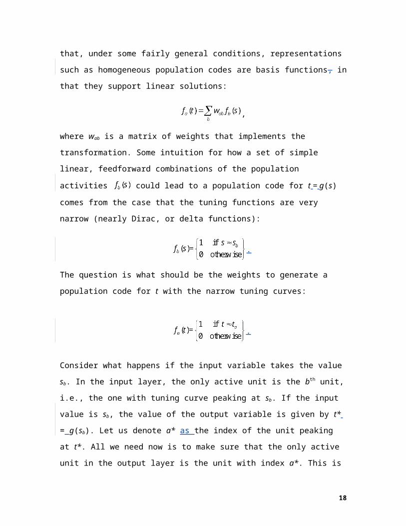
population code for s. It turns out that, under some fairly general conditions,

representations such as homogeneous population codes are basis functions, in that they

support linear solutions:

,

where wab is a matrix of weights that implements the transformation. Some intuition for

how a set of simple linear, feedforward combinations of the population activities

could lead to a population code for t = g(s) comes from the case that the tuning functions

are very narrow (nearly Dirac, or delta functions):

.

The question is what should be the weights to generate a population code for t with the

narrow tuning curves:

.

Consider what happens if the input variable takes the value sb. In the input layer, the only

active unit is the bth unit, i.e., the one with tuning curve peaking at sb. If the input value is

sb, the value of the output variable is given by t* = g(sb). Let us denote a* as the index of

the unit peaking at t*. All we need now is to make sure that the only active unit in the

output layer is the unit with index a*. This is done by setting the weight wa*b to one, and

11

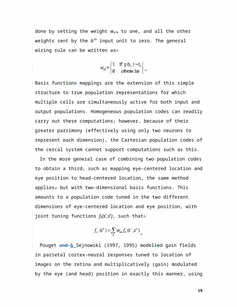
all the other weights sent by the bth input unit to zero. The general wiring rule can be

written as:

.

Basis functions mappings are the extension of this simple structure to true population

representations for which multiple cells are simultaneously active for both input and

output populations. Homogeneous population codes can readily carry out these

computations; however, because of their greater parsimony (effectively using only two

neurons to represent each dimension), the Cartesian population codes of the cercal system

cannot support computations such as this.

In the more general case of combining two population codes to obtain a third, such as

mapping eye-centered location and eye position to head-centered location, the same

method applies, but with two-dimensional basis functions. This amounts to a population

code tuned in the two different dimensions of eye-centered location and eye position,

with joint tuning functions fb(sr,se), such that:

.

Pouget and & Sejnowski (1997, 1995) modelled gain fields in parietal cortex-neural

responses tuned to location of images on the retina and multiplicatively (gain) modulated

by the eye (and head) position in exactly this manner, using tuning functions that are the

products of Gaussians for eye-centered position sr and monotonic sigmoids for eye

position se (for which preferred values are really points of inflectxion). In theory, one

would need a huge number of basis functions, one for each combination of preferred

value of eye-centered location and eye position;, but in practice, the actual number

depends on the required fidelity. Salinas and & Abbott (1995) proposed a similar scheme

and subsequently showed that these gain fields could arise from a standard network

model (Salinas & Abbott 1996). In this model, simple additive synaptic inputs to a

recurrently connected population, with excitatory synapses between similarly -tuned

neurons and inhibitory synapses between differently -tuned neurons, approximate a

12

product operation, which allowsing additive inputs from retinal position and eye position

signals to be combined multiplicatively.

Two aspects of these proposals make them incomplete as neural models. First is noise:

Eequations such as Equation 4 are true for the tuning functions themselves, but the

recorded activities are only noisy versions of these tuning functions. Second is the

unidirectional nature of the computation: Iin cases such as the parietal cortex, there is

nothing privileged about computing head-centered location from eye-centered location,

as the inverse computation sr = sh se is just as relevant (for instance, this computation is

required to predict the visual location of a sound source).

It is possible to solve the problem of noise using the recurrent network of the previous

section to eliminate the noise, effectively producing , and then using this in

computations such as eEquation . 4. However, Deneve et al. (2001) suggested a variant of

this recurrent network that solves the second problem too, thus combining noise removal,

basis function computation, and also cue integration in a population- coding framework.

In this final scheme, the inverse problems t = g(s) and s = g1(t) (or, in the case of the

parietal cortex, sh = sr + se and sr = sh se) are treated symmetrically. This implies the use

of a joint population code in all three variables, with tuning functions fa(sh, sr, se). From

this representation, population codes for any of the individual sh, sr, and se can be

generated as in eEquation . 5. In the recurrent maximum likelihood decoding scheme of

the previous section, there is a point along the bottom of the valley that represents any

value of the stimuli s = {sh, sr, se}. In Deneve et al.’s suggestion, the recurrent weights are

designed so that only values of s that satisfy the relationship sh = sr + se lie at the bottom

of the valley (which, in this case, has the structure of a two-dimensional plane). Thus,

only these values of s , and so these weights [AU: ok? NO, s is the subject in this case]are

stable points of the recurrent dynamics. Now, starting from noisy activity pattern, the

recurrent dynamics will lead to a smooth population code, which represents nearly the

maximum likelihood values of sh, sr, se that satisfy sh = sr + se, and thus solves any of the

three equivalent addition/subtraction problems.

Figure 3 shows an implementation of this scheme, including bidirectional weights

between the individual population codes and the joint population code. Crucially, tThe

recurrent dynamics work in such a crucial wayfashion that if there is no initial activity in

13

one of the population codes, say if only eye-centered and eye- position information is

available, then the position on the valley found by the network is determined only by the

noisy activities representing sr and se. This findingimplies that the network implements

noise removal and basis function computation. If noisy information about all three

variables is available, as in the case of cue integration (e.g., when an object can be seen

and heard at the same time), then the recurrent dynamics will combine them. If one

population has smaller activities than the others, then it will exert less influence over the

overall maximum likelihood solution. This ideaoutcome [AU: or better word?]is

statistically appropriate, if less- certain input variables are represented by lower

population activity (as they exactly are for the Poisson noise model for spiking, for which

the standard deviation of the activity of a neuron is equal to the square root of its mean).

Deneve et al. (2001) showed that this network could perform statistically near optimal

cue integration, together with coordinate transformation. Furthermore, the full, three-

dimensional, tuning functions in this scheme have very similar tuning properties to those

of parietal cells (Pouget et al. 2002).

1.3 Discussion of Standard Model

We have reviewed the standard models of Cartesian and homogeneous population codes,

showing how they encode information about stimulus variables, how information can be

decoded and used for discrimination, and how homogeneous population codes, because

of their close relationship with basis function approximation schemes, can support

nonlinear computations, such as coordinate transformations, and statistical computations,

such as cue integration. Dayan and & Abbott (2001) reviews most of the methods in more

detail.

Various issues about the standard model are actively debated. First, it might be thought

that population codes should have the characteristic of enabling the most accurate

decoding across a range of stimulus values. In fact, maximizing the Fisher information is

not always a good strategy, especially when short time windows are being considered

(Bethge et al. 2002). Moreover, non-homogeneity in tuning widths can improve coding

accuracy in some cases (Eurich & Wilke 2000).

A second area of active debate is the existence and effect of noise correlations (Abbott

& Dayan 1999, Oram et al. 1998, Pouget et al. 1999, Snippe & Koenderink 1992b,

14

Sompolinsky et al. 2001, Wilke & Eurich 2002, Wu et al. 2001, Yoon & Sompolinsky

1999). The little available experimental data suggests that correlations decrease

information content (Lee et al. 1998, Zohary et al. 1994), but theoretical studies have

shown that correlations can, in principle, greatly increase Fisher information (Abbott &

Dayan 1999, Oram et al. 1998, Sompolinsky et al. 2001, Wilke & Eurich 2002, Yoon &

Sompolinsky 1999). Also, decoding a correlated population code under the assumption

that the noise is independent (a common practice in experimental studies because

correlations are hard to measure) can (though need not necessarily) have dire deleterious

consequences on for decoding accuracy, and can even removeing the good properties of

the maximum likelihood estimator (Wu et al. 2001). [Peter: Wu et al show that

unfaithful decoding is actually not catastrophic].Another important issue for the recurrent network population coding methods is that it

is not reasonable to eliminate noise completely in the way we have discussed; rather,

population codes are continually noisy. It is thus important to assess the effect of

introducing noise into the recurrent dynamics, and to thusby understanding how it

propagates through the computations.

A final issue is that of joint coding. In the discussion of basis functions, we have

assumed that there are neurons with tuning functions that depend on all possible stimulus

variables, and with preferred values that are evenly distributed. This is obviously

implausible, and only some combinations can afford to be represented, perhaps in a

hierarchical scheme. In the case of V1, there are some ideas from natural scene statistics

(e.g. Li & Atick 1994) and also from general symmetry principles (e.g. Bressloff &

Cowan 2002) as to which combinations should exist; however, these have yet to be put

together with the basis function approximation schemes.

The standard model treats population codes as noisily representing certain information

about only one particular value of the stimulus s. This is a substantial simplification, and

in the next section, we consider recent extensions that require a radical change in the

conception of the population code.

2 ENCODING PROBABILITY DISTRIBUTIONS

2.1 Motivation

15

The treatment in the previous section has two main restrictions. First, we only considered

a single source of uncertainty coming from noisy neural activities, which is often referred

to as internal noise. In fact, as we see below, uncertainty is inherent in the structure of

most relevant computations, independent of the presence of internal noise. The second

restriction is that, although we considered how noise in the activities leads to uncertainty

in the Bayesian posterior distribution P[s|r] over a stimulus given neural responses, we

doid not consider anything other than estimating the single value underlying such a

distribution. Preserving and utilizing the full information contained in the posterior, such

as the uncertainty and possibly multi-modality, is computationally critical. We use the

term distributional population codes for population code representations of such

probability distributions.

In the computer vision literature, the way that uncertainty is inherent in computations

has been studied for quite some time in terms of “"ill-posed problems"” (Kersten 1999,

Marr 1982, Poggio et al. 1985). Most questions of interest that one may want to ask about

an image are ill-posed, in the sense that the images do not contain enough information to

provide unambiguous answers. Perhaps the best-known example of such an ill-posed

problem is the aperture problem in motion processing. When a bar moves behind an

aperture, there is an infinite number of 2D motions consistent with the image (Figure

4A). In other words, the image by itself does not specify unambiguously the motion of

the object. This may appear to be a highly artificial example, sincebecause most images

are not limited to bars moving behind apertures. Yet, this is a real problem for the

nervous system because all visual cortical neurons see the world through the apertures of

their visual receptive fields. Moreover, similar problems arise in the computation of the

3D structure of the world, the localization of auditory sources, and many other

computations (Knill & Richards 1996).

Figure 4 (A) The aperture problem. Two successive snapshots (at time t and t + 1)

of an edge moving behind an aperture. An infinite number of motion vectors is

consistent with this image sequence, some of them shown with red arrows. (B)

Probability distribution over all velocities given the image sequence shown in

(A). All velocities have zero probability except for the ones corresponding to the

black line, which have an equal non-zero probability. (C) Same as in (A) but for

16

noisy images of a blurred moving contour. This time, possible motions differ not

only in direction but also in speed. (D) The corresponding probability

distribution takes the form of an approximately gaussian ridge whose width is a

function of the noise and blurring level in the image sequence.

What can be done to deal with this uncertainty? The first part of the solution is to adopt

a probabilistic approach. Within this framework, we no longer seek a single value of the

variable of interest, since this does not exist; rather, perception is conceived as statistical

inference giving rise to probability distributions over the values. For the aperture

problem, the idea is to recover the probability distribution over all possible motions s

given the sequence of images I. This posterior distribution P[s|I] is analogous to the

posterior distribution P[s|r] over the stimulus s, given the responses that we discussed

above, except that uncertainty here does not arise from the fact that multiple stimuli can

lead to the same neural responses due owing to internal noise, but rather, it comes from

the fact that many different underlying motions give rise to the same observed image. For

In the case of no strong prior and a simple bar moving behind an aperture, the posterior

distribution takes the form indicated in Figure 4B. Only the motions lying on a particular

line in a 2D plane of velocities have non-zero probabilities; all are equally likely in the

absence of any further information.

This is actually an idealized case. In reality, the image itself is likely to be corrupted by

noise, and the moving object may not have very well- defined contours. For instance,

Figure 4C shows two snapshots of a blurred contour moving through an aperture. This

time, the speed, as well as the direction of the stimulus, is ambiguous. As a result, the

posterior becomes a diffuse (e.g., Gaussian) ridge instead, centered on the idealized line

(Figure 4D).

These posterior probability distributions capture everything there is to know about the

variables of interest given the image. This[AU: what does ‘this’ refer to? Reword as

shown] leads to aAt least two critical questions then arise: dDoes the brain work with

probability distributions? And, if so, how are they encoded in neural activities? The first

part of this section reviews psychophysical evidence suggesting that the answer to the

first question is very likely to be yes. These experiments attempt to refute the null

17

hypothesis that only a single aspect of such distributions (such as their means or the

locations of their peaks) plays any role in perception, as opposed to an alternative

hypothesis that other information, notably the width of the distributions, is also

important. Having established the importance of distributional encoding, we will

consider how populations of neurons might encode, and compute, probability

distributions. We then study some experimental neurobiological evidence supporting this

view, and finally discuss how these probabilistic population codes can be used for

computation.

Psychophysical Evidence

Many experiments support the notion that perception is the result of a statistical inference

process (Knill & Richards 1996). Perhaps one of the simplest demonstrations of this

phenomenon is the way that contrast influences speed perception. It has been known for

quite some time that the perceived speed of a grating increases with contrast (Blakemore

& Snowden 1999, Stone & Thompson 1992, Thompson 1982). This effect is easy to

explain within a probabilistic framework. The idea is that the nervous system seeks the

posterior distribution of velocity given the image sequence, obtained through Bayes rule:

.

In this example, the prior distribution P[s] represents any prior knowledge the nervous

system has about the velocity of objects in the real world, independently of any particular

image. For convenience, we consider velocity in only one dimension (say horizontal for

a vertical grating, thus eliminating the aperture problem). Experimental measurements

suggest that the prior distribution of 1D velocity in movies of natural scenes takes the

form of a Gaussian distribution centered at zero ([AU: first initial? R.]dDe RuytersRuyter

van Steveninck, personal communation;, red curve in Figure 4A5A). In other words, in

natural movies, most motions tend to be slow. Note that the observation that slow

motions tend to be more common in real images is independent of seeing any particular

image, which is precisely what the prior is about.

To compute the likelihood P[I|s] as a function of s, one needs to know the type of

noise corrupting natural movies, and its dependence on contrast (Weiss et al. 2002).

Fortunately, we do not need to venture into those technical details, as intuitive notions are

18

sufficient. The likelihood always peaks near the veridical velocity. However, the width of

this peak (compared to its height) is a function of the extent to which the presented image

outweighs the noise. This is a function of contrast; as the contrast increases, the image

more strongly outweighs the noise, and the peak gets narrower (compare the green curve

in Figure 4A 5A and B).

Given this knowledge of the prior and likelihood functions, we can examine the

posterior distribution over velocity, which is simply proportional to the product of these

two functions (Equation 6). At high contrast, the posterior distribution peaks at about the

same velocity as the likelihood function, because the likelihood function is narrow and

dominates the product. At low contrast, the likelihood function widens, and the product is

more strongly influenced by the prior. Since Because the prior favors slow speeds, the

result is a posterior peaking at slower velocity than the likelihood function. If the

perceived velocity corresponds to either the peak (mode), or the mean, of the posterior

distribution, it is clear that it[AU: what? The prreceived velocity, how about this

wording?I’m not sure it should be repeated.] will clearly decrease with contrast.

Experimental evidence concerning human perception of speed directly follows this

prediction (Blakemore & Snowden 1999, Hurlimann et al. 2002, Stone & Thompson

1992, Thompson 1982). Note that to model this effect, it is critical to have a

representation of the likelihood function, or at least its width. If we knew only its peak

position, it would be impossible to reproduce the experimental data, sincebecause the

peak remains at the same position across contrast. Such experiments provide compelling

evidence that the nervous system, by some means, represents probability distributions.

This example alone is not an ironclad proof, but what is remarkable is that this basic

set of assumptions (i.e., with no additional parameters) can account for a very wide large

body of experimental data regarding velocity perception---, a feat that no other model can

achieve (Weiss et al. 2002).

There are many other demonstrations as to how perception can be interpreted as a

statistical inference problem requiring the explicit manipulation of uncertainty (Jacobs

2002, Knill 1998, Knill & Richards 1996). One compelling example concerns how

humans combine visual and haptic cues to assess the shape of objects (Ernst & Banks

2002). In this experiment, subjects were asked to judge the height of a bar, which they

19

could see and touch. First, subjects viewed with both eyes a visual stimulus consisting of

many dots, displayed as if glued to the surface of the bar. To make the task harder, each

dot was moved in depth away from the actual depth of the bar, according to a noise term

drawn from a Gaussian distribution. As the width of the noise distribution was increased,

subjects found it harder and harder to estimate the height of the bar accurately. Ernst and

& Banks (2002) suggested that observers recover a posterior distribution over heights

given the visual image, and that this distribution widens as the noise in the image

increases. Next, haptic information as to the height was also provided through a force-

feedback robot, allowing subjects the chance to integrate it with the variably uncertain

visual information. Ernst and & Banks reported that humans behave as predicted by

Bayes law in combining visual and haptic information. That is, in estimating the height of

the bar, subjects take into account the reliability of the two different cues. This again

suggests that the human brain somehow represents and manipulates the widths of the

likelihood functions for vision and touch.

2.2 Encoding and Decoding Probability Distributions 

Several schemes have been proposed for encoding and decoding probability distributions

in populations of neurons. As for the standard account covered in the first section of this

reviewof section 1, there is a difference between mechanistic and descriptive models.

Mechanistic models set out to explain the sensory processing path by which neurons

come to code for aspects of a probability distribution. The only example of this that we

consider is the log likelihood model of Weiss and & Fleet (2002). Descriptive models,

which are our main focus, offer a more abstract account of the activities of cells, ignoring

the mechanistic details. There are also important differences in the scope of the models.

Some, such as the gain and log-likelihood models, are more or less intimately tied to the

idea that the only important aspect of uncertainty is the width of a single peaked

likelihood (which often translates into the variance of the distribution). Others, more

ambitiously, attempt to represent probability distributions in rich and multi-modal glory.

2.2.1 LOG-LIKELIHOOD METHOD A major question for distributional population

codes is where the distributions come from?. Sensory organs sense physical features of

the external world, such as light or sound waves, not probability distributions. How are

the probability distributions inferred from photons or sound waves? Weiss and & Fleet

20

(2002) have suggested a very promising answer to this question. They considered the

motion-energy filter model, which is one of the most popular accounts of motion

processing in the visual system (Adelson & Bergen 1985). Under their interpretation, the

activity of a neuron tuned to prefer velocity v (ignoring its other preferences for retinal

location, spatial frequency, etc.) is viewed as reporting the logarithm of the likelihood

function of the image given the motion, log(P[I|v]). This suggestion is intrinsically

elegant, neatly providing a statistical interpretation for conventional filter theory. Further,

in the case that there is only a single motion in the image, decoding only involves the

simple operation of (summing and) exponentiating to find the full likelihood. A variety of

schemes for computing based on the likelihood are made readily possible by this scheme,

although some of these require that the likelihood only have one peak for them to work.

2.2.2 GAIN ENCODING FOR GAUSSIAN DISTRIBUTIONS We have already

met the simplest distributional population code. When a Bayesian approach is used to

decode a population pattern of activity (Equation 3), the result is a a posterior distribution

P[s|r] over the stimulus. If the noise in the response of neurons in a large population is

assumed to be independent, the law of large numbers dictates that this posterior

distribution converges to a Gaussian (Papoulis 1991). Like any Gaussian distribution, it

is fully characterized by its mean and standard deviation. The mean of this posterior

distribution is controlled by the position of the noisy hill of activity. If the noisy hill is

centered around a different stimulus value, so will be the posterior distribution. By

contrast, when the noise follows a Poisson distribution, the standard deviation of the

posterior distribution is controlled by the amplitude of the hill. These effects are

illustrated in Figure 6 (see color insert). [AU: you don’t appear to have called out Figure

5. Please call it out before Figure 6 is called out. We called out Fig 4 rather than Fig 5

above by mistake.]

Figure 5 Bayesian estimation of the speed of an object moving at 10 deg/s for low

and high contrast. For visual clarity, the amplitudes of all distributions have been

normalized to one (A). At low contrast, the likelihood function (light gray curve)

is wide because the image provides unreliable data about the motion. When this

likelihood function is multiplied with the prior (dotted curve) to obtain the

21

posterior distribution (solid black curve), the peak of the posterior distribution

(arrow) ends up indicating a slower speed than the veridical speed (10 deg/s). (B)

For a high contrast, the likelihood function is narrower, because the image

provides more reliable information. As a result, the posterior distribution is

almost identical to the likelihood function and peaks closer to the veridical speed.

This could explain why humans perceive faster speeds for higher contrasts.

This observation [AU: what? observation, finding? observation] implies that the gain

of the population activity controls the standard deviation of the posterior distribution,

which is the main quantity required to account for the simple psychophysical examples

above. For instance, that lower contrast leads to lower population activities is exactly a

mechanistic implementation of increased uncertainty in the quantity encoded.

This method is subject to some strong limitations. In particular, although one can

imagine a mechanism that substitutes carefully chosen activities for the random Poisson

noise so that the posterior distribution takes on a different form, the central limit theorem

argument above implies that it is not a viable way of encoding distributions other than

simple Gaussians.

2.2.3 CONVOLUTION ENCODING For non-Gaussian distributions P[s|I] (strictly

densities) that cannot be characterized by a few parameters such as their means and

variances, more complicated solutions must be devised. One possibility inspired by the

encoding of nonlinear functions is to represent the distribution using a convolution code,

obtained by convolving the distribution with a particular set of kernel functions.

The canonical kernel is the sine, as used in Fourier transforms. Most nonlinear

functions of interest can be recovered from their Fourier transforms, which implies that

they can be characterized by their Fourier coefficients. To specify a function with

infinite accuracy one needs an infinite number of coefficients, but for most practical

applications, a few coefficients suffice (say, 50 or so). One could therefore use a large

neuronal population of neurons to encode any function by devoting each neuron to the

encoding of one particular coefficient. With N neurons, ignoring noise and negative firing

rates, one can encode N coefficients. The activity of neuron a is computed by taking the

22

dot product between a sine function assigned to that neuron and the function being

encoded (as is done in a Fourier transform):

,

where neuron a is characteriszed by its parameters wa and .

Many other kernel functions may be used for convolution codes. For instance, one

could use Gaussian kernels, in which case the activity of the neurons is obtained through:

.

Gaussian kernels are usually better than sine kernels for learning and computation when

the distributions are concentrated around one or a small number of values.

If a large population of neurons is used, and their Gaussian kernels are translated

copies of one another, eEquation 7 becomes a discrete convolution. In other words, the

pattern of activity across the neuronal population is simply the original distribution,

filtered by a Gaussian kernel.

Note that when there is no uncertainty associated with the encoded variable, i.e., the

encoded probability distribution is a Dirac function, P[s|I] = (s,s*), eEquation 7 reduces

to:

.

This is simply the equation for the response to orientation s* of a neuron with a Gaussian

tuning curve centered on sa. In other words, the classical framework we reviewed in the

first half of this paper is a subcase of this more general approach.

With the convolution code, one solution to decoding is to use deconvolution, a linear

filtering operation which that reverses the application of the kernel functions. There is no

exact solution to this problem; buthowever, a close approximation to the original function

can be obtained by applying a band pass filter, which typically takes the form of a

Mexican hat kernel. The problem with this approach is that it fails miserably when the

23

original distribution is sharply peaked, such as a Dirac function. Indeed, a band pass filter

cannot recover the high frequencies, which are critical for sharply peaked functions.

Moreover, linear filters do not perform well in the realistic case of noisy encoding

neurons.

Anderson (1994) took this approach a step further, making the seminal suggestion of

convolutional decoding rather than convolutional encoding. In one version of this scheme

(which bears an interesting relationship to the population vector), activity ra of neuron a is

considered to be a vote for a particular (usually probabilistic) decoding basis function

Pa[s]. Then, the overall distribution decoded from r is

.

The advantage of this scheme is the straightforward decoding model; one disadvantage is

the concomitant difficulty of encoding. A second disadvantage of this scheme is shared

with the linear deconvolution approach: Iit cannot readily recover the high frequencies

that are important for sharply peaked distributions P[s|I], which arise in the case of ample

information in I.

An alternative to these linear decoding schemes for convolution codes, which is

consistent with the theme of this review, is to adopt a probabilistic approach. For

instance, given the noisy activity of a population of neurons, one should not try to recover

the most likely value of s, but rather the most likely distribution over s, P[s|I] (Zemel et

al. 1998). This can be achieved using a nonlinear regression method such as the

Expectation-Minimization Maximization altgorithm[AU: Is it standard for this to be

capitalized? Yes - it's often called just EM] (Dempster et al. 1977).

In the decoding schemes of both Anderson and Zemel et al., the key concept is to treat

a population pattern of activity as a representation of a probability distribution, as

opposed to a single value (as is done in the standard approach reviewed in the first

section). To see the difference, consider a situation in which the neurons are noise free. If

the population code is encoding a single value, we can now recover the value of s with

absolute certainty. In the case of Anderson and Zemel et al, we can now recover the

distribution, P[s|I], with absolute certainty. As discussed earlier, in many real-world

24

situations P[s|I] is not a Dirac function;, so optimal decoding recovers the distribution

P[s|I] with absolute certainty, but the inherent uncertainty about s remains.

One trouble problem with the convolutional encoding (and indeed the other encodings

that we have described) is that there is no systematic way of representing multiple values

as well as uncertainty. For instance, a wealth of experiments on population coding is

based on random dot kinematograms, for which some fraction of the dots move in

randomly selected directions, with and the rest (the correlated dots) moveing in one

particular direction, which is treated as the stimulus s*. It is not obviously reasonable to

treat this stimulus as a probability distribution P[s|I] over a single direction s (with a peak

at s*), since, in fact, there is actual motion in many directions. Rather, the population

should be thought of encoding a weighting or multiplicity function (s), which indicates

the strength of direction s in the stimulus. We consider below a particularly interesting

case of this below (Treue et al. 2000), in which multiplicity functions were used to probe

motion metamers.

In some situations both multiple values and uncertainty apply. Consider viewing a

random grating kinematogram through an aperture: wWhat should be encoded is actually

a distribution P[(s)|I] over possible functions (s), given the image sequence I. [AU:

first initials?] M. Sahani and P. Dayan (manuscript in preparationsubmission) noted this

problem, and suggested a variant of the convolution code, called the doubly distributional

population code (DDPC), to cope with this., In their scheme, the mean activity of neuron

a (to be compared with that of eEquation 7) comes from averaging the convolutional

encoding of the multiplicity functions (s) over the distribution P[(s)|I]

.

Here, ga() is an activation function which that must be non-linear in order for the scheme

to work correctly. Decoding is more complex still, but demonstrably effective at least in

simple cases. ([AU: first initials?] M. Sahani and P. Dayan, manuscript in preparation).

2.3 Examples in Neurophysiology

In this section we review some neurophysiological studies that pertain to the hypothesis

that neurons encode probability distributions. The case of the log likelihood encoding

25

scheme is particularly straightforward, sincebecause it amounts to a probabilistic

interpretation of motion-energy filters, and there is ample evidence that such filters offer

at least a close approximation to the responses of neurons in area V1 and MT (Adelson &

Bergen 1985, Emerson et al. 1992).

Since Because it is only fairly recently that neurophysiologists have started testing

whether neurons encode probability distributions, evidence relating to other coding

schemes is limited. In almost all cases, the tests have been limited to probability

distributions over a set of discrete possibilities such as two particular directions of motion

rather than a probability density function over a continuous variable like motion velocity.

We thus treat this case first.

2.3.1 UNCERTAINTY IN 2-AFC EXPERIMENTS Gold & Shadlen et al. (2001)

have trained monkeys to indicate whether a visual stimulus is moving in one of two

possible directions, e.g., up or down (Gold & Shadlen 2001). In this 2-alternative forced

choice (2-AFC) experiment, the stimulus was composed of a set of moving dots, some

moving randomly and the rest moving either up or down, depending on the trial. The

difficulty of the task can be controlled by changing the percentage of the dots moving

coherently upward, or downward.

The optimal strategy for the nervous system is to pick the motion with the highest

probability given the activity r of the motion- sensitive neurons in early visual areas,.

Tthat is, to decide that motion is upward if: . Applying Bayes

Rule, we can rewrite the test in terms of log-ratios:

The term (above) on the right-hand side is a constant that depends on the conditions of

the experiment; in Shadlen's experiment, the two motions were equally likely, so this

term was 0. This equation shows that a Bayesian decision process only requires

comparing the term on the left-hand side, the log likelihood ratio, against a fixed

threshold. The exact relationship between single- cells responses and the log likelihood

ratio remains to be precisely established, but Shadlen's data suggest that neurons in

26

parietal and frontal “"association cortex"”, in particular in areas LIP (lateral intra parietal)

or the FEF (frontal eye field) [AU: please spell out these terms once], may represent the

log likelihood ratio (see Gold & Shadlen 2001 for an overview). This is some of the first

experimental evidence suggesting that association areas are indeed representing and

manipulating probabilities.

A second set of experiments also pertains to this hypothesis. Anastasio et al. (2000)

have recently proposed that superior colliculus neurons compute the probability that a

stimulus is present in their receptive field given the image, ,

where xi and yi are the eye-centered coordinates of the cell's receptive field. Note that this

probability distribution is defined over a binary variable, which can take only the value

“'present'” or “'absent'.” Therefore, a neuron only needs to encode one number, say

, because the other probability, ], is constrained to follow

the relation . Anastasio et al. suggested that this is

indeed what collicular neurons do: Ttheir activity is proportional to .

Evidence for their hypothesis derives from the responses of multimodal collicular

neurons, which appear to be using Bayes rule when combining visual and auditory inputs.

This is indeed the optimal strategy for multimodal integration if the neurons are

representing probability distributions.

Platt and & Glimcher (1999) have made a related proposal in the case of LIP neurons.

They trained monkeys to saccade to one of two possible locations while manipulating the

prior probabilities of those locations. They found that responses of sensory and motor LIP

neurons are proportional to the prior probability of making a saccade to the location of

the particular cell's receptive field. In addition, they manipulated the probability of

reward for each saccade and found that neuronal responses are proportional to the reward

probability.

None of these examples deals with continuous variables. However, they offer

preliminary evidence that neurons represent probability distributions or related quantities,

such as log likelihood ratios. Is there any evidence that neurons go the extra step and

actually encode continuous distributions at the population level, using any of the schemes

reviewed above? Is representing probability distributions a general feature of all cortical

27

areas? As far as we know, thoese questions have not been directly addressed with

experimental techniques. However, as we review below, some data are already strongly

supporting a probabilistic interpretation of cortical activity in all areas.

2.3.1 EXPERIMENTS SUPPORTING GAIN ENCODING Does the brain use the

gain of the responses of population codes to represent certainty? In other words, as the

reliability of a stimulus is increased, is it the case that the gain of its population code in

the brain increases as well? The answer appears to be yes in some cases. For instance, as

the contrast of an image increases, visual features, such as orientation, and direction of

motion or color, can be estimated with higher certainty. This higher certainty is reflected

in the cortex by the fact that the gain of neurons increases with contrast. This is true in

particular in the case of orientation, or direction of motion, for which contrast is known to

have a purely multiplicative effect (Dean 1981, McAdams & Maunsell 1999, Sclar &

Freeman 1982, Skottun et al. 1987). Loudness of sounds plays a similar role to contrast in

audition and also controls the gain of auditory neurons. It is important to keep in mind

that an increase in gain implies an increase in reliability only for certain noise

distributions. For instance, it is true for independent noise following a Poisson

distribution (or the near-Poisson distribution typically found in cortex). In the case of

contrast, the noise does remain near-Poisson regardless of the contrast in the image

(McAdams & Maunsell 1999). Unfortunately, the noise is certainly not independent (Lee

et al. 1998, Zohary et al. 1994), and, worse, we do not know how the correlations are

affected by contrast. It is also not clear how the neural mechanisms interpreting the

population activity treat the increased gain. It is therefore too early to tell for sure

whether gain is used to encode reliability,; but given the improvement in performance on

perceptual tasks as contrast is increased (e.g. Regan & Beverley 1985), it seems a

reasonable hypothesis.

2.3.2 EXPERIMENTS SUPPORTING CONVOLUTION CODES According to the

convolution code scheme, the profile of activity across the neuronal population should

closely mimic the profile of the encoded distribution, since it is simply a filtered version

of the distribution. Therefore, as a stimulus becomes more unreliable, that is, as its

probability distribution widens, the population pattern of activity should also widen. We

saw that this was not the case with contrast: aAs contrast decreases, the gain of the

28

population patterns of activity decreases but the width remains identical (at least in the

case in which it has been measured, like orientation).

However, in other cases, this scheme might be at work. For instance, it is known that

humans are much better at localizing visual targets than auditory ones, which indicatesing

that vision is more reliable than audition (at least in broad day light). Interestingly,

sSpatial receptive fields of visual neurons tend to be much smaller than the spatial

receptive field of auditory neurons. This interesting tendency implies that population

patterns of activity for visual stimuli are sharper than those for sounds. If these patterns

are low pass versions of the underlying distributions, the posterior distribution for visual

stimuli is narrower than the one for auditory stimuli (Equation. 7), which would account

for the fact that visual stimuli are more reliably localized.

A number of physiological studies on transparent motion also provide support for the

convolution code hypothesis. Stimuli composed of two patterns sliding across each other

can create the impression of two separate surfaces moving in different directions. The

general neurophysiological finding is that an MT cell's response to these stimuli can be

characterized as the average of its responses to the individual components (Recanzone et

al. 1997, van Wezel et al. 1996). This is consistent with the convolution of the cell's

tuning function with a multi-modal distribution, with peaks corresponding to the two

underlying directions of motion.

2.3.3 EXPERIMENTS SUPPORTING DDPC Transparent motion experiments not

only provide support for convolution coding, but also for doubly distributional population

codes (DDPC). In a recent experiment, Treue et al. (2000) monitored the response of

motion sensitive neurons while manipulating the distribution of motion in random

kinematograms. For instance, they tested neurons with a display in which half of the dots

move coherently in one direction and the other half move coherently in another direction.

In this case, the motion multiplicity function is simply the sum of two Dirac functions

peaking at the two positions, respectively. They also employed more complicated

multiplicities in other experiments, including up to five separate motions. In each case,

they found that the responses of MT neurons could be roughly approximated as following

a relationship of the form of Eequation 8, albeit with a hint that the activity across the

whole population may be normalized rather than involving individual non-linearities.

29

In other cases such as binocular rivalry (Blake 2001), multiplicity in input stimuli leads

to (alternating) perceptual selection rather than transparency. However, there is

neurophysiological evidence (Blake & Logothetis 2002, Leopold & Logothetis 1996) that

an equivalent of transparency may be operating at early stages of visual processing,

whose an account of which would require a theory of the form of DDPC.

2.4 Computations Using Probabilistic Population Codes

The psychophysical evidence we have reviewed earlier, such as the effect of contrast on

velocity perception, suggests that the brain not only represents probability distributions,

but also manipulates and combines these distributions according to Bayes rule (or a

reasonably close approximation). A few models have examined how neural networks

could implement Bayes rule for the various encoding schemes that have been proposed.

As an example, we once again use the experiment performed by Ernst and & Banks

(2002). Recall that this experiment required subjects to judge the width of a bar. The

optimal strategy in this case consists of recovering the posterior distribution over the

width, w, given the image (V) and haptic (H) information. As usual this is done using

Bayes rule:

.

This simple example shows that we need two critical ingredients to perform Bayesian

inferences in cortical networks: a representation of the prior and likelihood functions,

and a mechanism to multiply the distributions together.

If we use a convolution code for all distributions, we can simply multiply all the

population codes together term by term. This calculation automatically leads to a pattern

of activity corresponding to a convolved version of the posterior (Fig.ure 7, see color

insert). This solution requires neurons that can multiply their inputs, a readily achievable

neural operation (Chance et al. 2002, Salinas & Abbott 1996). If we consider neurons as

representing the logarithm of the probability distributions, as suggested by Weiss and &

Fleet (2002), then Bayes rule only requires adding the distributions together (because the

30

logarithm of a product is simply the sum of the individual logarithms). Addition is

another basic operation that neurons can easily perform.

When the probability distributions are encoded using the position and gain of

population codes, the only solution that has been proposed so far is that of Deneve et al.,

(2001), which we reviewed in the first half of this manuscriptpaper. This approach has

three major limitations. First, it does not currently incorporate prior probabilities; second,

it works only with Gaussian distributions; and third, the network only computes the peak

of the posterior but not the posterior itself. This last limitation comes from the fact that

the stable hills in this model are noise-free and have fixed amplitudes (Figure, 3, see

color insert). As such they can only encode the mean of the posterior distribution but not

its variance. This makes it hard to use the network to represent uncertainty in

intermediate computations.

On the other hand, this solution has several advantages. First, it performs a Bayesian

inference using noisy population codes, whereasile, in the previous schemes, it remains to

be seen whether multiplication or addition of distributions can be performed robustly in

the presence of noise. In fact, the assumption of variability in the Deneve et al. (2001)

approach is key: iIt is used to encode the certainty associated with each variable. In other

words, in this network, noise is a feature allowing the system to perform Bayesian

inferences.

The other advantage of this network is that it can deal with more general inferences

than those investigated by Ernst and & Banks (2002). In their experiment, touch and

vision are assumed to provide evidence for the same variable, namely, the width of the

bar. In the coordinate transform problem investigated by Deneve et al., the evidence

comes in different frames of reference: eye-centered for vision and head-centered for

audition. Therefore, the various sources of evidence must be remapped into a common

format before they can be combined. This is a very general problem in cue integration:

eEvidence rarely comes commonly encoded, and must be remapped first. A classical

example is depth perception, which relies on widely different cues such as shading,

stereopsis, and shape from motion, each involving its own representational scheme. In

Deneve et al.'s network, remapping is performed through the basis function layer.

31

Whether, and how, such remappings could be performed using convolution or log codes

is presently unknown.

3 CONCLUSION

Population codes are coming of age as representational devices, in that there is a widely

accepted standard encoding and decoding model together with a mature understanding of

its properties. However, there remain many areas of active investigation. One in

particular one that we have highlighed is the way that continuous attractor networks are

ideally suited to implement important computations with population codes, including

noise removal, basis function approximations, and statistically sound cue integration.

Another focus has been population codes for more general aspects of stimulus

representations, including computational uncertainty and multiplicity. With the notable

exception of the log likelihood model of Weiss and & Fleet (2002), which shows how

motion-energy filters provide an appropriate substrate for statistical computations, these

proposals are more computational than mechanistic. However, the inexorable inundation

of psychophysical results showing the sophisticated ways that observers extract, learn,

and manipulate uncertainty, acts as a significant spur to the further refinement and

development of such models.

ACKNOWLEDGMENTS

[AU: do you wish to thank or acknowledge anyone?] We are grateful to Sophie Deneve,

Peter Latham, Jonathan Pillow, Maneesh Sahani and Terrence Sejnowski for their

collaboration on various of the studies mentioned. Funding was from the NIH (AP), the

Gatsby Charitable Foundation (PD) and the ONR (RSZ).

REFERENCES

Abbott L, Dayan P. 1999. The effect of correlated variability on the accuracy of a

population code. Neural Comput. 11:91--101

Adelson EH, Bergen JR. 1985. Spatiotemporal energy models for the perception of

motion. J. Opt. Soc. Am. A 2:284--99

32

Anastasio TJ, Patton PE, Belkacem-Boussaid K. 2000. Using Bayes' rule to model

multisensory enhancement in the superior colliculus. Neural Comput. 12:1165--87

Andersen R, Essick G, Siegel R. 1985. Encoding of spatial location by posterior parietal

neurons. Science 230:456--58

Anderson C. 1994. Neurobiological computational systems. In Computational

Intelligence Imitating Life, pp. 213--22. New York: IEEE Press

Ben-Yishai R, Bar-Or RL, Sompolinsky H. 1995. Theory of orientation tuning in visual

cortex. Proc. Natl. Acad. Sci. USA 92:3844--48

Bethge M, Rottermund D, Pawelzik K. 2002. Optimal short-term population coding:

when Fisher information fails. Neural Comput. 14:2317--52

Bishop CM. 1995. Neural Networks for Pattern Recognition. Oxford, UK: Oxford Univ.

Press

Blake R. 2001. A primer on binocular rivalry, including current controversies. Brain

Mind 2:5--38

Blake R, Logothetis NK. 2002. Visual competition. Nat. Rev. Neurosci. 3(1):13--21

Blakemore MR, Snowden RJ. 1999. The effect of contrast upon perceived speed: a

general phenomenon? Perception 28:33--48

Borst A, Theunissen FE. 1999. Information theory and neural coding. Nat. Neurosci.

2:947--57

Bressloff P, Cowan JD. 2002. The visual cortex as a crystal. Physica D. In press

173 :226-258 (2002). [AU: update?]

Brunel N, Nadal JP. 1998. Mutual information, Fisher information, and population

coding. Neural Comput. 10:1731--57

Chance FS, Abbott LF, Reyes AD. 2002. Gain modulation from background synaptic

input. Neuron 35:773--82

Cohen M, Grossberg S. 1983. Absolute stability of global pattern formation and parallel

memory storage by competitive neural network. IEEE Trans. SMC 13:815--26

Compte A, Brunel N, Goldman-Rakic PS, Wang XJ. 2000. Synaptic mechanisms and

network dynamics underlying spatial working memory in a cortical network model.

Cereb. Cortex 10:910--23

Dayan P, Abbott LF. 2001. Theoretical Neuroscience. Cambridge, MA: MIT Press

33

Dean AF. 1981. The relationship between response amplitude and contrast for cat striate

cortical neurones. J. Physiol. 318:413--27

DeGroot MH. 1970. Optimal Statistical Decisions.[AU: location of publisher?] New

York, NY: McGraw-Hill

Dempster AP, Laird NM, Rubin DB. 1977. Maximum likelihood from incomplete data

via the EM algorithm. J. R. Stat. Soc. B39:1--38

Deneve S, Latham P, Pouget A. 1999. Reading population codes: a neural

implementation of ideal observers. Nat. Neurosci. 2:740—45[AU: I don’t see where

you’ve cited this. Please cite in text or delete here. Thanks.It was cited but under

Pouget et al. This is now fixed.]

Deneve S, Latham P, Pouget A. 2001. Efficient computation and cue integration with

noisy population codes. Nat. Neurosci. 4:826--31

Emerson RC, Bergen JR, Adelson EH. 1992. Directionally selective complex cells and

the computation of motion energy in cat visual cortex. Vis. Res. 32:203--18

Ernst MO, Banks MS. 2002. Humans integrate visual and haptic information in a

statistically optimal fashion. Nature 415:429--33

Eurich CW, Wilke SD. 2000. Multidimensional encoding strategy of spiking neurons.

Neural Comput. 12:1519--29

Foldiak P. 1993. The 'ideal homunculus': statistical inference from neural population

responses. In Computation and Neural Systems, ed. F Eeckman, J Bower, pp. 55--60.

Norwell, MA: Kluwer Acad. Publ.

Georgopoulos A, Kalaska J, Caminiti R. 1982. On the relations between the direction of

two-dimensional arm movements and cell discharge in primate motor cortex. J.

Neurosci. 2:1527--37

Gershon ED, Wiener MC, Latham PE, Richmond BJ. 1998. Coding strategies in monkey

V1 and inferior temporal cortices. J. Neurophysiol. 79:1135--44

Gold JI, Shadlen MN. 2001. Neural computations that underlie decisions about sensory

stimuli. Trends Cogn. Sci. 5:10--16

Graziano MS, Andersen RA, Snowden RJ. 1994. Tuning of MST neurons to spiral

motions. J. Neurosci. 14:54--67

34

Green DM, Swets JA. 1966. Signal Detection Theory and Psychophysics.Los Altos,

CA[AU: location of publisher?]: Wiley

Heeger DJ. 1992. Normalization of cell responses in cat striate cortex. Vis. Neurosci.

9:181--97

Hol K, Treue S. 2001. Different populations of neurons contribute to the detection and

discrimination of visual motion. Vis. Res. 41:685--89

Hopfield JJ. 1982. Neural networks and physical systems with emergent collective

computational abilities. Proc. Natl. Acad. Sci. USA 79:2554--58

Hubel D, Wiesel T. 1962. Receptive fields, binocular interaction and functional

architecture in the cat's visual cortex. J. Physiol. (Lond.) 160:106--54

Hurlimann F, Kiper D, Carandini M. 2002. Testing the Bayesian model of perceived

speed. Vis. Res. 42:2253-7[AU: only one page?]

Jacobs RA. 2002. What determines visual cue reliability? Trends Cogn. Sci. 6:345--50

Kersten D. 1999. High level vision as statistical inference. In The New Cognitive

Neurosciences, ed. MS Gazzaniga. Cambridge: MIT Press

Knill DC. 1998. Surface orientation from texture: ideal observers, generic observers and

the information content of texture cues. Vis. Res. 38:1655--82

Knill DC, Richards W. 1996. Perception as Bayesian Inference. New York: Cambridge

Univ. Press

Lee C, Rohrer WH, Sparks DL. 1988. Population coding of saccadic eye movements by

neurons in the superior colliculus. Nature 332:357--60

Lee D, Port NL, Kruse W, Georgopoulos AP. 1998. Variability and correlated noise in

the discharge of neurons in motor and parietal areas of the primate cortex. J. Neurosci.

18:1161--70

Leopold DA, Logothetis NK. 1996. Activity-changes in early visual cortex reflect

monkeys' percepts during binocular rivalry. Nature 379:549--53

Li Z, Atick JJ. 1994. Toward a theory of the striate cortex. Neural Comput. 6:127--46

Marr D. 1982. Vision. Cambridge, MA: MIT Press

Maunsell JHR, Van Essen DC. 1983. Functional properties of neurons in middle

temporal visual area of the macaque monkey. I. Selectivity for stimulus direction,

speed, and orientation. J. Neurophysiol. 49:1127--47

35

Mazzoni P, Andersen R. 1995. Gaze coding in the posterior parietal cortex. In The

Handbook of Brain Theory, ed. M Arbib, pp. 423--26. Cambridge, MA: MIT Press

McAdams CJ, Maunsell JRH. 1999. Effects of attention on orientation-tuning functions

of single neurons in macaque cortical area V4. J. Neurosci. 19:431--41

Nelson ME. 1994. A mechanism for neuronal gain control by descending pathways.

Neural Comput. 6:242--54

O'Keefe J, Dostrovsky J. 1971. The hippocampus as a spatial map. Preliminary evidence

from unit activity in the freely moving rat. Brain Res. 34:171--75

Oram M, Foldiak P, Perrett D, Sengpiel F. 1998. The 'Ideal Homunculus': decoding

neural population signals. Trends Neurosci. 21:359-365[AU: only one page?]

Papoulis A. 1991. Probability, Random Variables, and Stochastic Process. New York

[AU: Place of publication?]McGraw-Hill

Paradiso M. 1988. A theory of the use of visual orientation information which exploits

the columnar structure of striate cortex. Biol. Cybern. 58:35--49

Perrett DI, Smith PA, Potter DD, Mistlin AJ, Head AS, et al. 1985. Visual cells in the

temporal cortex sensitive to face view and gaze direction. Proc. R. Soc. Lond. B Biol.

Sci. 223:293--317

Platt ML, Glimcher PW. 1999. Neural correlates of decision variables in parietal cortex.

Nature 400:233--38

Poggio T. 1990. A theory of how the brain might work. Cold Spring Harbor Symp.

Quant. Biol. 55:899--910

Poggio T, Torre V, Koch C. 1985. Computational vision and regularization theory.

Nature 317:314--19

Pouget A, Deneve S, Ducom J, Latham P. 1999. Narrow vs wide tuning curves: What's

best for a population code? Neural Comput. 11:85--90

Pouget A, Deneve S, Duhamel JR. 2002. A computational perspective on the neural basis

of multisensory spatial representations. Nat. Rev. Neurosci. 3:741--47

Pouget A, Sejnowski T. 1997. Spatial transformations in the parietal cortex using basis

functions. J. Cogn. Neurosci. 9:222--37

36

Pouget A, Sejnowski TJ. 1995. Spatial representations in the parietal cortex may use

basis functions. In Advances in Neural Information Processing Systems, ed. G

Tesauro, DS Touretzky, TK Leen. Cambridge, MA: MIT Press

Pouget A, Thorpe S. 1991. Connectionist model of orientation identification. Connect.

Sci. 3:127--42

Pouget A, Zhang K, Deneve S, Latham PE. 1998. Statistically efficient estimation using

population codes. Neural Comput. 10:373--401

Recanzone G, Wurtz R, Schwarz U. 1997. Responses of MT and MST neurons to one

and two moving objects in the receptive field. J. Neurophysiol. 78:2904--15

Regan D, Beverley K. 1985. Postadaptation orientation discrimination. J. Opt. Soc. Am.

[A] 2:147--55

Rieke F, Warland D, De Ruyter van Steveninck R, Bialek W. 1999. Exploring the Neural

Code. Cambridge: MIT Press

Salinas E, Abbot L. 1994. Vector reconstruction from firing rate. J. Comput. Neurosci.

1:89--107

Salinas E, Abbot L. 1995. Transfer of coded information from sensory to motor

networks. J. Neurosci. 15:6461--74

Salinas E, Abbott LF. 1996. A model of multiplicative neural responses in parietal cortex.

Proc. Natl. Acad. Sci. USA 93:11,956--61

Sanger T. 1996. Probability density estimation for the interpretation of neural population

codes. J. Neurophysiol. 76:2790--93

Sclar G, Freeman R. 1982. Orientation selectivity in the cat's striate cortex is invariant

with stimulus contrast. Exp. Brain Res. 46:457--61

Seung H. 1996. How the brain keeps the eyes still. Proc. Natl. Acad. Sci. USA

93:13,339--44

Seung H, Sompolinsky H. 1993. Simple model for reading neuronal population codes.

Proc. Natl. Acad. Sci. USA 90:10,749--53

Shadlen M, Britten K, Newsome W, Movshon T. 1996. A computational analysis of the

relationship between neuronal and behavioral responses to visual motion. J. Neurosci.

16:1486--510

37

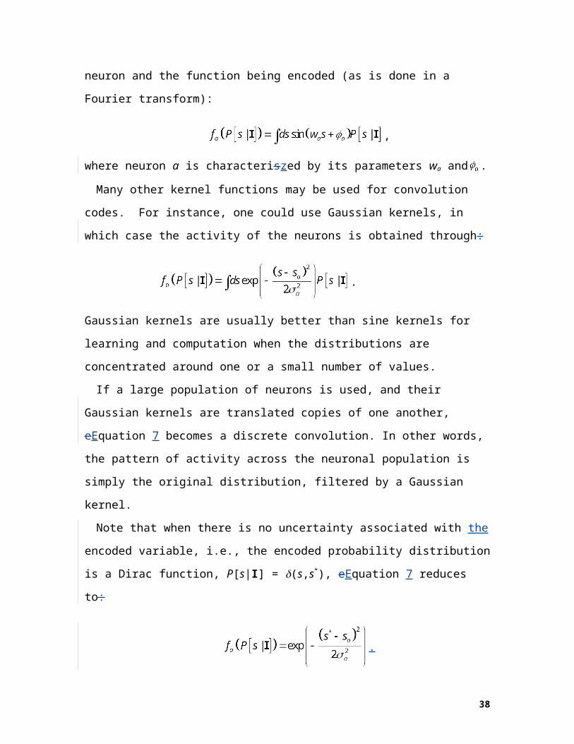
Skottun BC, Ohzawa I, Sclar G, Freeman RD. 1987. The effects of contrast on visual

orientation and spatial frequency discrimination: a comparison of single cells and

behavior. J. Neurophysiol. 57:773--86

Snippe HP, Koenderink JJ. 1992a. Discrimination thresholds for channel-coded systems.

Biol. Cybern. 66:543--51

Snippe HP, Koenderink JJ. 1992b. Information in channel-coded systems: correlated

receivers. Biol. Cybern. 67:183--90

Sompolinsky H, Yoon H, Kang K, Shamir M. 2001. Population coding in neuronal

systems with correlated noise. Phys. Rev. E Station. Nonlinear Soft Matter Phys.

64:051904

Stone LS, Thompson P. 1992. Human speed perception is contrast dependent. Vis. Res.

32:1535--49

Theunissen F, Miller J. 1991. Representation of sensory information in the cricket cercal

sensory system. II. Information theoretic calculation of system accuracy and optimal

tuning-curve widths of four primary interneurons. J. Neurophysiol. 66:1690--703

Thompson P. 1982. Perceived rate of movement depends on contrast. Vis. Res. 22:377--

80

Tolhurst D, Movshon J, Dean A. 1982. The statistical reliability of signals in single

neurons in cat and monkey visual cortex. Vis. Res. 23:775--85

Treue S, Hol K, Rauber H. 2000. Seeing multiple directions of motion-physiology and

psychophysics. Nat. Neurosci. 3:270--76

van Wezel RJ, Lankheet MJ, Verstraten FA, Maree AF, van de Grind WA. 1996.

Responses of complex cells in area 17 of the cat to bi-vectorial transparent motion.

Vis. Res. 36:2805--13

Weiss Y, Fleet DJ. 2002. Velocity likelihoods in biological and machine vision. In

Statistical Theories of the Cortex, ed. R Rao, T SejnowskiB, Olshausen, M.S. Lewicki,

[AU: page range? Not available77-96]. Cambridge: MIT Press

Weiss Y, Simoncelli EP, Adelson EH. 2002. Motion illusions as optimal percepts. Nat.

Neurosci. 5:598--604

Wilke SD, Eurich CW. 2002. Representational accuracy of stochastic neural populations.

Neural Comput. 14(1):155--89

38

Wu S, Nakahara H, Amari S. 2001. Population coding with correlation and an unfaithful

model. Neural Comput. 13:775--97

Yoon H, Sompolinsky H. 1999. The effect of correlations on the {F}isher information of

population codes. In Advances in Neural Information Processing Systems, ed. MS

Kearns, S Solla, DA Cohn, pp. 167--73. Cambridge, MA: MIT Press

Zemel R, Dayan P, Pouget A. 1998. Probabilistic interpretation of population code.

Neural Comput. 10:403--30

Zhang K. 1996. Representation of spatial orientation by the intrinsic dynamics of the

head-direction cell ensemble: a theory. J. Neurosci. 16:2112--26

Zohary E, Shadlen M, Newsome W. 1994. Correlated neuronal discharge rate and its

implication for psychophysical performance. Nature 370:140--43

39