Embed Size (px)
Citation preview
Enabling the Use of Heterogeneous Computing for Bioinformatics.
Ramakrishna Bijanapalli Chakri
Thesis submitted to the Faculty of theVirginia Polytechnic Institute and State University
in partial fulfillment of the requirements for the degree of
Master of Sciencein
Computer Engineering
Peter M. Athanas, ChairWu-chun Feng
Allan Dickerman
September 16, 2013Blacksburg, Virginia
Keywords: FPGA, Hardware Acceleration, High Performance Computing, DNAAlignment, LabVIEW, Heterogeneous Computing, GP-GPUs.
Copyright 2013, Ramakrishna Bijanapalli Chakri

Enabling the Use of Heterogeneous Computing for Bioinformatics
Ramakrishna Bijanapalli Chakri
(ABSTRACT)
The huge amount of information in the encoded sequence of DNA and increasing interestin uncovering new discoveries has spurred interest in accelerating the DNA sequencing andalignment processes. The use of heterogeneous systems, that use di↵erent types of compu-tational units, has seen a new light in high performance computing in recent years; Howeverexpertise in multiple domains and skills required to program these systems is causing anhindrance to bioinformaticians in rapidly deploying their applications into these heteroge-neous systems. This work attempts to make an heterogeneous system, Convey HC-1, withan x86-based host processor and FPGA-based co-processor, accessible to bioinformaticians.First, a highly e�cient dynamic programming based Smith-Waterman kernel is implementedin hardware, which is able to achieve a peak throughput of 307.2 Giga Cell Updates per Sec-ond (GCUPS) on Convey HC-1. A dynamic programming accelerator interface is providedto any application that uses Smith-Waterman. This implementation is also extended toGeneral Purpose Graphics Processing Units (GP-GPUs), which achieved a peak throughputof 9.89 GCUPS on NVIDIA GTX580 GPU. Second, a well known graphical programmingtool, LabVIEW is enabled as a programming tool for the Convey HC-1. A connection isestablished between the graphical interface and the Convey HC-1 to control and monitor theapplication running on the FPGA-based co-processor.
This work was supported in part by the I/UCRC Program of the National Science Foundation(NSF) within the NSF Center for High-Performance Reconfigurable Computing (CHREC),Grant No. IIP-0804155.

Dedication
I dedicate this work to my parents and to my uncle & aunt who brought me up.
iii
Acknowledgments
This thesis would not have been possible without the guidance and help of several individuals.I would like to take this opportunity to acknowledge them.
First and foremost, I would like to express my sincere gratitude to my advisor, Dr. PeterAthanas, for giving me the opportunity to be a part of the Configurable Computing Lab(CCM). He has been an immense source of inspiration to me throughout the process. I amgrateful for his patience and his continued support of me at every stage of my academic lifeat Virginia Tech. It would have been great to pursue a course work taught by him, which Iunfortunately could not take.
Dr. Alan Dickerman and Dr. Wu-chun Feng, for graciously agreeing to serve on my thesiscommittee on a short notice. I also had the privilege of taking the computer architecturecourse taught by Dr Feng, which was inspiring and provided me with a great learning expe-rience.
Dr. Krzystof Kepa, for his valuable insights and for helping me complete my work on time.It was great to meet a person with strong dedication and amazing wit like him.
David Uliana, for all his help over the two years, for inviting me to his home for a thanksgivingdinner and introducing me to his warm and generous family members.
Shaver Deyerle, for all the fun we had together and for the insightful interactions on severalacademic and non academic matters.
Kavya Shagrithaya, for introducing me to this lab, for helping me choose my course workand for guiding me during my admission process.
My other lab mates: Ali, for all the endless conversations about the world of technology,Tannous, for all the advice and technical support in using my lab computer, Andrew, forincluding me in his meal plan at D2 over the summer and for sharing several interestingfacts on daily basis, Ritesh, for being supportive as a batch-mate and giving me companyand support on various issues over the two years, Kaiwan, for his generous help and forbeing very approachable anytime I seek information from him, Kevin, for his support duringthe project and all the valuable interactions we had. My former lab members Abhay andUmang, for their support and guidance.
iv

All my CCM lab mates for all the endless fun we had with bike rides, Foosball tournaments,picnics and lunch at El Rodeo and Happy Wok. Members of Wearable lab for their supporton various occasions, particularly Jacob for driving his pickup truck to help me move.
The administrative sta↵ of the Graduate School and the Bradley Department of Electricaland Computer Engineering for their timely help and cooperation.
My amazing friends at Virginia Tech, Apoorva, Aruna, Dilip, Harish, Rashmi, Shuchi,Supratik and many others, for their support in every aspect of my academic life here. Mynumerous other friends in various parts of the world for extending their help from far.
My parents, my uncle and aunt, my siblings and my cousins for their unconditional love andsupport during my graduate school life.
Last but not the least, God for showering His blessings on me.
v

Contents
List of Figures ix
List of Tables xi
1 Introduction 1
1.1 Motivation . . . . . . . . . . . . . . . . . . . . . . . . . . . . . . . . . . . . . 1
1.2 Contributions . . . . . . . . . . . . . . . . . . . . . . . . . . . . . . . . . . . 2
1.3 Organization . . . . . . . . . . . . . . . . . . . . . . . . . . . . . . . . . . . 3
2 Background 4
2.1 DNA Sequencing . . . . . . . . . . . . . . . . . . . . . . . . . . . . . . . . . 4
2.2 Sequence Alignment . . . . . . . . . . . . . . . . . . . . . . . . . . . . . . . 5
2.2.1 Indexing Based Approach . . . . . . . . . . . . . . . . . . . . . . . . 5
2.2.2 Burrows Wheeler Transform Based Approach . . . . . . . . . . . . . 5
2.2.3 Dynamic Programming and Smith-Waterman . . . . . . . . . . . . . 6
2.3 Field Programmable Gate Arrays . . . . . . . . . . . . . . . . . . . . . . . . 7
2.3.1 FPGA Architecture . . . . . . . . . . . . . . . . . . . . . . . . . . . . 8
2.3.2 FPGA Tools . . . . . . . . . . . . . . . . . . . . . . . . . . . . . . . . 9
2.3.3 Programming FPGAs . . . . . . . . . . . . . . . . . . . . . . . . . . . 9
2.4 Convey HC-1 . . . . . . . . . . . . . . . . . . . . . . . . . . . . . . . . . . . 10
2.4.1 Host Processor . . . . . . . . . . . . . . . . . . . . . . . . . . . . . . 10
2.4.2 Application Engine Hub (AEH) . . . . . . . . . . . . . . . . . . . . . 10
vi

2.4.3 Application Engines (AEs) . . . . . . . . . . . . . . . . . . . . . . . . 12
2.4.4 Dispatch Interface . . . . . . . . . . . . . . . . . . . . . . . . . . . . 12
2.4.5 Memory Interface . . . . . . . . . . . . . . . . . . . . . . . . . . . . . 13
2.4.6 Management Interface . . . . . . . . . . . . . . . . . . . . . . . . . . 13
2.4.7 Personality . . . . . . . . . . . . . . . . . . . . . . . . . . . . . . . . 14
2.5 LabVIEW FPGA . . . . . . . . . . . . . . . . . . . . . . . . . . . . . . . . . 15
2.6 GP-GPUs and CUDA . . . . . . . . . . . . . . . . . . . . . . . . . . . . . . 16
2.6.1 Streaming Multiprocessors and CUDA Cores . . . . . . . . . . . . . . 17
2.6.2 CUDA Memories . . . . . . . . . . . . . . . . . . . . . . . . . . . . . 17
2.7 Related Work . . . . . . . . . . . . . . . . . . . . . . . . . . . . . . . . . . . 19
2.7.1 Attempts for Hardware Acceleration of Bioinformatics Applications . 19
2.7.2 Work on GP-GPUs . . . . . . . . . . . . . . . . . . . . . . . . . . . . 20
2.7.3 Unconventional Hardware Programming . . . . . . . . . . . . . . . . 21
3 High Performance Smith-Waterman Implementation 23
3.1 Smith-Waterman Processing Element . . . . . . . . . . . . . . . . . . . . . . 23
3.2 Systolic Array . . . . . . . . . . . . . . . . . . . . . . . . . . . . . . . . . . . 24
3.3 FIFO Interface . . . . . . . . . . . . . . . . . . . . . . . . . . . . . . . . . . 26
3.4 Dispatch Interface . . . . . . . . . . . . . . . . . . . . . . . . . . . . . . . . . 26
3.5 Interface to the Bio-applications . . . . . . . . . . . . . . . . . . . . . . . . . 27
3.6 General Purpose-GPUs . . . . . . . . . . . . . . . . . . . . . . . . . . . . . . 28
3.6.1 One Thread per Cell . . . . . . . . . . . . . . . . . . . . . . . . . . . 28
3.6.2 One Thread per Row . . . . . . . . . . . . . . . . . . . . . . . . . . . 28
4 Convey-LabVIEW Interface 30
4.1 LabVIEW FPGA Communication . . . . . . . . . . . . . . . . . . . . . . . . 30
4.2 Connections and Bit-Mapping . . . . . . . . . . . . . . . . . . . . . . . . . . 31
4.3 Simulation of ConVI . . . . . . . . . . . . . . . . . . . . . . . . . . . . . . . 32
4.4 LabVIEW HDL Wrapper . . . . . . . . . . . . . . . . . . . . . . . . . . . . . 32
vii

4.5 Designing using LabVIEW . . . . . . . . . . . . . . . . . . . . . . . . . . . . 36
5 Results and Analysis 38
5.1 High Performance Smith-Waterman . . . . . . . . . . . . . . . . . . . . . . . 38
5.1.1 Area Occupancy . . . . . . . . . . . . . . . . . . . . . . . . . . . . . 39
5.1.2 Bandwidth Requirements . . . . . . . . . . . . . . . . . . . . . . . . . 43
5.1.3 Simulation . . . . . . . . . . . . . . . . . . . . . . . . . . . . . . . . . 45
5.2 Performance with GP-GPU . . . . . . . . . . . . . . . . . . . . . . . . . . . 45
5.3 Performance Compared With Recent Work . . . . . . . . . . . . . . . . . . . 48
5.4 LabVIEW Convey Interface . . . . . . . . . . . . . . . . . . . . . . . . . . . 49
5.4.1 Comparing ConVI with Bflow . . . . . . . . . . . . . . . . . . . . . . 50
5.4.2 Comparison with OpenCL Smith-Waterman . . . . . . . . . . . . . . 50
6 Conclusion and Future Scope 51
6.1 Dynamic Programming Environment on Convey . . . . . . . . . . . . . . . . 51
6.1.1 Burrows-Wheeler Aligner Smith-Waterman (BWASW) . . . . . . . . 52
6.1.2 BLAT like Fast and Accurate Search Tool (BFAST) . . . . . . . . . . 53
6.2 Dynamic Parallelism using Kepler GP-GPUs . . . . . . . . . . . . . . . . . . 53
6.3 Unified Programming with LabVIEW for Convey . . . . . . . . . . . . . . . 54
Bibliography 55
A Smith-Waterman State Machine 60
B Smith-Waterman PE and Pipeline Modules 63
C Smith-Waterman Host Code 65
D LabVIEW HDL Connection 69
viii

List of Figures
2.1 Smith-Waterman Alignment Score Matrix. . . . . . . . . . . . . . . . . . . . 7
2.2 Convey Architecture. Source: [1]. Used under fair use guidelines, 2011. . . . 11
2.3 Convey AE Hub and the Dispatch Interface. Source: [2]. Used under fair useguidelines, 2011. . . . . . . . . . . . . . . . . . . . . . . . . . . . . . . . . . . 12
2.4 Convey Memory Connections. Source: [2]. Used under fair use guidelines, 2011. 14
2.5 Convey Management interface with Signals. Source: [2]. Used under fair useguidelines, 2011. . . . . . . . . . . . . . . . . . . . . . . . . . . . . . . . . . . 15
2.6 NVIDIA GP-GPU Architecture. . . . . . . . . . . . . . . . . . . . . . . . . . 17
3.1 A single Smith-Waterman Processing Element. . . . . . . . . . . . . . . . . . 24
3.2 Cascading of the Smith-Waterman PEs. . . . . . . . . . . . . . . . . . . . . 25
3.3 Hierarchical design of PEs and their interface to FIFOs in each of the AEs. . 25
3.4 FIFO Interface . . . . . . . . . . . . . . . . . . . . . . . . . . . . . . . . . . 26
3.5 Final structure of the Smith-Waterman design showing the connections to thememory and the dispatch on Convey HC-1. . . . . . . . . . . . . . . . . . . . 27
3.6 One Thread per cell. . . . . . . . . . . . . . . . . . . . . . . . . . . . . . . . 28
3.7 One Thread per Row. . . . . . . . . . . . . . . . . . . . . . . . . . . . . . . . 29
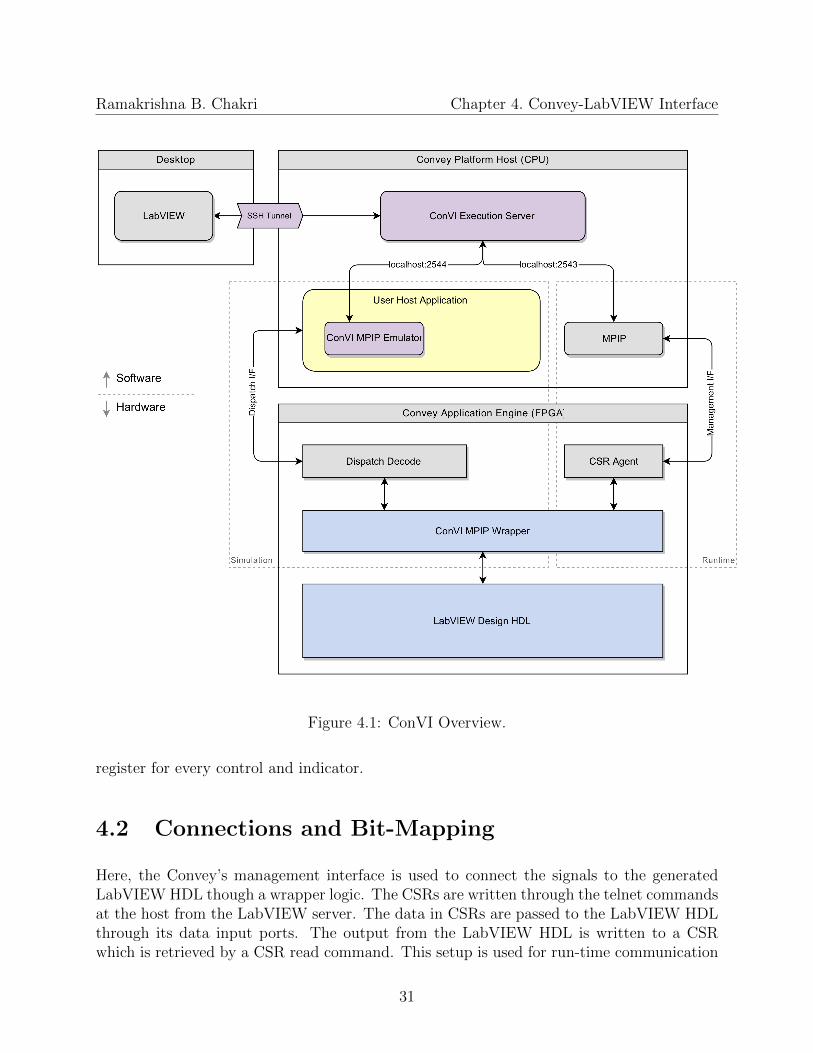
4.1 ConVI Overview. . . . . . . . . . . . . . . . . . . . . . . . . . . . . . . . . . 31
4.2 Non-blocking copcall in Convey assembly code . . . . . . . . . . . . . . . . . 33
4.3 Wrapper interfacing LabVIEW-generated HDL to Convey’s top-level CAE pers. 35
4.4 Smith-Waterman PE designed using LabVIEW. . . . . . . . . . . . . . . . . 36
4.5 A 16-PE pipeline generated using LabVIEW VI Scripting. . . . . . . . . . . 37
ix
4.6 LabVIEW front panel with controls and indicators for Smith-Waterman ap-plication running on Convey HC-1. . . . . . . . . . . . . . . . . . . . . . . . 37
5.1 Resource consumption by the Smith-Waterman accelerator on Convey HC-1. 39
5.2 Resource allocation for each of the components in the design. . . . . . . . . . 42
5.3 Timing diagram showing the alignment score calculations. . . . . . . . . . . 44
5.4 The output of the accelerator: the sequence numbers with the scores of theirpairwise alignment. . . . . . . . . . . . . . . . . . . . . . . . . . . . . . . . . 45
5.5 Kernel speedup with number of target and search sequences over x86. . . . . 46
5.6 Overall speedup attained by using the GP-GPU over x86 processor. . . . . . 47
5.7 Throughput comparison of recent work on high performance Smith-WaterImplementation. . . . . . . . . . . . . . . . . . . . . . . . . . . . . . . . . . . 49
6.1 Proposed BWA-SW on Convey HC systems. . . . . . . . . . . . . . . . . . . 52
6.2 Proposed BFAST on Convey HC systems. . . . . . . . . . . . . . . . . . . . 53
x
List of Tables
2.1 Convey HC-1 Specifications . . . . . . . . . . . . . . . . . . . . . . . . . . . 11
2.2 The AEs Compared . . . . . . . . . . . . . . . . . . . . . . . . . . . . . . . . 13
4.1 Request and Response formats . . . . . . . . . . . . . . . . . . . . . . . . . . 32
4.2 The Bit Mapping for LabVIEW Commands through 64-bit CSR and AEGRegisters. . . . . . . . . . . . . . . . . . . . . . . . . . . . . . . . . . . . . . 34
5.1 Key features of the platforms used . . . . . . . . . . . . . . . . . . . . . . . 46
5.2 Performance comparison with related work on heterogeneous computers. . . 48
xi

Chapter 1
Introduction
Genomics is one of the emerging fields that o↵ers a huge challenge to both biologists andcomputer scientists due to the magnitude of data involved in a genome. For instance, thehuman genome has three billion nucleotide base pairs, and it holds a great deal of information.This huge amount of data requires constant processing for researchers all over the world tomake new discoveries in the field of genomics. These computationally intensive problemstake up a huge amount of time to execute on a serial computer. Programmers all overthe world are trying to find new ways to accelerate this process, either by formulating newalgorithms or by deploying them on unconventional systems and custom hardware to solvethese problems.
Heterogeneous computing systems are an example for these unconventional systems. Thesesystems use a variety of di↵erent types of computational units like a Graphics ProcessingUnit (GPU), a co-processor, or a Field-Programmable Gate Array (FPGA) along with aCentral Processing Unit (CPU). Unfortunately, these heterogeneous systems bring in newand unexplored territories to bioinformaticians and programmers, making it arduous forthem to rapidly deploy applications on these heterogeneous platforms.
1.1 Motivation
This work is motivated by the fact that the heterogeneous systems based on FPGAs witha high potential for reconfigurability and application acceleration has been out of reach ofbioinformaticians. Programming the accelerator requires training in digital logic design,expertise in HDL programming and a working knowledge of heterogeneous architecturesincluding several interfaces that are specific to these machines.
Some of the prior work involving the use of heterogeneous architectures for bioinformaticshave been made primarily for benchmarking the performance of the machine and is of little
1

Ramakrishna B. Chakri Chapter 1. Introduction
use for the bioinformaticians. The hardware design engineer lacks the skills to deciphervarious biological requirements and parameters, which brings the need for bioinformaticiansto use the low level hardware interfaces from the accelerator in their applications.
The Virginia Bioinformatics Institute (VBI) owns several nodes of FPGA-based heteroge-neous computers from Convey Computers called HC-1 and HC-1ex. Convey demonstrateda huge performance gain with a dynamic programming based alignment algorithm calledSmith-Waterman, on their HC-1ex platform [3]. This work involves the development of ac-celerator for Smith-Waterman. The following are the reasons for designing a custom versionof dynamic programming personality.
1. Dynamic programming kernels can be mapped e�ciently in hardware by employingsystolic arrays.
2. A custom design can be altered for one’s own benefits.
3. This can be used as a template to implement any dynamic programming solutionby modifying the source thats already there. Ex Needleman-Wunch [4] , CLUSTAL,GeneScan.
4. Applications can be created in the host that make use of dynamic programming inhardware. Algorithms such as BWASW [5], Swift [6] and BFAST [7] directly useSmith-Waterman. There could be several other such algorithms that benefit from anaccelerator for dynamic programming.
Need for an Unconventional ApproachUse of conventional approach to programming heterogeneous systems involves skills in multi-ple programming paradigms and is complicated by di↵erent platforms and di↵erent program-ming languages. The components of the heterogeneous systems often involve sub-systemsintegrated from di↵erent vendors. These often lead to di�culty in timing, synchronizationand handshake protocols. All of these problems inherent in these system provide a hindranceto bio-scientists from using them. Thus, providing a intuitive and unified solution to pro-gram the heterogeneous systems enables the bioinformaticians to develop applications forthese systems.
1.2 Contributions
In this work, a two-fold approach to solve the problem is proposed. One approach is to useheterogeneous architectures for bioinformatics. Several levels of possible optimization weremade to achieve highest performance achievable. The other approach is to use unconventionalmethods to make this huge computation power available to computational biologists.
2

Ramakrishna B. Chakri Chapter 1. Introduction
For the first task, a highly e�cient dynamic programming kernel for Smith-Waterman isbuilt. Interfaces are defined and tested for its functionality. This interface is made availableto any application that requires dynamic programming. The performance is compared witha serial computer as well as with a similar implementation on General Purpose-GraphicsProcessing Units (GP-GPUs).
For the second task, a versatile and mature graphical programming language is chosen. Itis made to work with an heterogeneous environment and tested for the functionality. Acommunication channel is formed between the Graphical User Interface (GUI) based front-end and a back-end design running on the heterogeneous system. This is finally tested fromend-to-end with hardware simulation as well as the run-time execution.
1.3 Organization
The crux of this thesis consists of four major chapters which is organized as follows,
Chapter 2 - Background: This chapter familiarizes the concepts behind DNA sequencingand alignments, FPGA architecture, programming and its tools, Convey architecture and itspersonality development environment, LabVIEW and its FPGA programming capabilities,and finally the General Purpose Graphics Processing Units and its programming paradigm,CUDA.
This chapter also highlights some of the previous work in the field of hardware based accel-erations for bioinformatics applications, GP-GPU based Smith-Waterman implementationsand graphical and high level programming models for hardware.
Chapter 3 - High Performance Smith-Waterman Implementation: The implemen-tation of first part of the contribution along with the approach taken, is provided in thischapter. This chapter details the implementation of the Smith-Waterman cell to the finalintegration with the Convey memory. This chapter ends with a description of the implemen-tation of the Smith-Waterman algorithm on GP-GPUs.
Chapter 4 - Convey LabVIEW Interface: The implementation of the second part of thecontribution along with the approach taken is provided in this chapter. This chapter containselaborate details on the LabVIEW generated HDL, its interface to the Convey environmentand finally its connections to the LabVIEW VI front panel through specific interfaces.
Chapter 5 - Results and Analysis: This chapter exhibits the results obtained, and theanalysis of those results. The performance of the FPGA based Smith-Waterman is comparedto that of the GP-GPU. Finally it compares this work with some of the previous work donein this area.
3

Chapter 2
Background
2.1 DNA Sequencing
DNA carries the genetic information in the cell and is capable of self-replication and synthesisof RNA. DNA consists of two long chains of nucleotides twisted into a double helix andjoined by hydrogen bonds between the complementary bases adenine (A) and thymine (T)or cytosine (C) and guanine (G). In order to read and analyze any genetic sequence, biologistsmust first determine a sample DNA sequence by reading the sequence of nucleotide basesand must compare them to a reference or a known genome. Since the human DNA is a threebillion base pair sequence, this becomes a di�cult computational problem.
To determine the sequence of base pairs, the DNA sample is first replicated to produceapproximately thirty copies of the original DNA sequence. The copies of the replicated se-quence are then cut at random points throughout the entire length of the genome, producingshort lengths of intact chains of base pairs known as short reads [8]. DNA sequencing tech-nology began with Sanger sequencing in 1977 and evolved to many new massively parallelsequencing technologies such as Illumina. The Illumina/Solexa sequencing technology typi-cally produces 50 to 200 million 32 to 100 base pair reads on a single run of the machine [9].However, other new sequencing techniques such as Roche/454 sequencing technology has pro-duced long reads > 400 base pair in production, Illumina is gradually increasing read length> 100 base pair, and Pacific Bioscience generates 1000 base pair reads in early testing [5]requiring a need for both short and long read alignments.
These massively parallel sequencing technologies produce a large volume of short reads, thatmapping all these short reads to a large genome presents a great demand to develop fastersequence alignment programs.
4
Ramakrishna B. Chakri Chapter 2. Background
2.2 Sequence Alignment
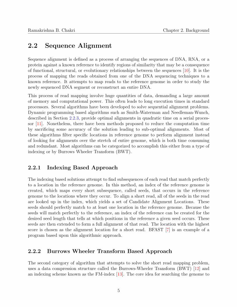
Sequence alignment is defined as a process of arranging the sequences of DNA, RNA, or aprotein against a known reference to identify regions of similarity that may be a consequenceof functional, structural, or evolutionary relationships between the sequences [10]. It is theprocess of mapping the reads obtained from one of the DNA sequencing techniques to aknown reference. It attempts to map reads to the reference genome in order to study thenewly sequenced DNA segment or reconstruct an entire DNA.
This process of read mapping involve huge quantities of data, demanding a large amountof memory and computational power. This often leads to long execution times in standardprocessors. Several algorithms have been developed to solve sequential alignment problems.Dynamic programming based algorithms such as Smith-Waterman and Needleman-Wunch,described in Section 2.2.3, provide optimal alignments in quadratic time on a serial proces-sor [11]. Nonetheless, there have been methods proposed to reduce the computation timeby sacrificing some accuracy of the solution leading to sub-optimal alignments. Most ofthese algorithms filter specific locations in reference genome to perform alignment insteadof looking for alignments over the stretch of entire genome, which is both time consumingand redundant. Most algorithms can be categorized to accomplish this either from a type ofindexing or by Burrows Wheeler Transform (BWT).
2.2.1 Indexing Based Approach
The indexing based solutions attempt to find subsequences of each read that match perfectlyto a location in the reference genome. In this method, an index of the reference genome iscreated, which maps every short subsequence, called seeds, that occurs in the referencegenome to the locations where they occur. To align a short read, all of the seeds in the readare looked up in the index, which yields a set of Candidate Alignment Locations. Theseseeds should perfectly match to at least one location in the reference genome. Because theseeds will match perfectly to the reference, an index of the reference can be created for thedesired seed length that tells at which positions in the reference a given seed occurs. Theseseeds are then extended to form a full alignment of that read. The location with the highestscore is chosen as the alignment location for a short read. BFAST [7] is an example of aprogram based upon this algorithmic approach.
2.2.2 Burrows Wheeler Transform Based Approach
The second category of algorithm that attempts to solve the short read mapping problem,uses a data compression structure called the Burrows-Wheeler Transform (BWT) [12] andan indexing scheme known as the FM-index [13]. The core idea for searching the genome to
5

Ramakrishna B. Chakri Chapter 2. Background
find the exact alignment for a read is rooted in the su�x trie theory [14]. The BWT of asequence of characters is constructed by creating a square matrix containing every possiblerotation of the desired string, with one rotated instance of the string in each row. The ma-trix is then sorted lexicographically, and the BWT is the sequence of characters in the lastcolumn, starting from the top.
This solution uses the FM-index, a data structure that synergistically combines the Burrows-Wheeler transform and the su�x array, to e�ciently store information required to traversea su�x tree for a reference sequence. These solutions can quickly find a set of matchinglocations in a reference genome for short reads that match the reference genome with a limitednumber of di↵erences. However, the running time of this class of algorithm is exponentialwith respect to the allowed number of di↵erences; therefore BWT-based algorithms tend tobe less sensitive than others. Bowtie and BWA [9] are examples of programs based uponthis algorithmic approach.
2.2.3 Dynamic Programming and Smith-Waterman
The problem of sequence alignment can be characterized to be solved by dynamic program-ming algorithms where the bigger problem is broken into smaller similar problems. Becauseof the similar nature of the smaller problems, one can take advantage of a highly data parallelhardware designs. It is especially beneficial when a large amount of data has to be processedwhile dealing with long sequences or a large number of smaller sequences.
Dynamic programming is used in many areas of computing and finds a great application infinding best alignments in genome sequences. The disadvantages of DNA alignments usingdynamic programming are quadratic time and space complexities [15]. The use of parallelexecution can reduce the time complexity to linear time. One solution is to use a highly dataparallel processor like a GPU. Another solution is to design a specific processing kernel inhardware and replicate it several times using a FPGA. These solutions can achieve massiveamounts of parallelism. Hence FPGAs and GPUs form an excellent platform for genomealignment using dynamic programming.
Smith-Waterman [16], based on dynamic programming, is the one of the popular algorithmsfor finding local alignments given a query and a reference sequence. It calculates the scorematrix for two given sequences using the equations 2.1a to 2.1d that describe the working ofthe algorithm. It involves the use of a score matrix that keeps the track of the scores as thecomputations are being done. The alignments are performed by tracing the path from thehighest score in the matrix to a point where the score drops to zero. This is termed as thetrace-back. Figure 2.1 shows the alignment of two sequences TTTACGT and GCCACCGTwith the score matrix for the alignment and its trace-back. Based on the score matrix, thethreshold point is chosen from where the trace-back starts to find all the possible optimal
6

Ramakrishna B. Chakri Chapter 2. Background
Figure 2.1: Smith-Waterman Alignment Score Matrix.
alignments.
H(i, 0) = 0, 0 i m.......................................................................................... (2.1a)
H(0, j) = 0, 0 j n.......................................................................................... (2.1b)
if ai = bj then w(ai, bj) = w(match) or if ai 6= bj then w(ai, bj) = w(mismatch) (2.1c)
H(i, j) = max
8>>><
>>>:
0 ,
H(i� 1, j � 1) + w(ai, bj) Match/Mismatch,
H(i� 1, j) + w(ai,�) Deletion,
H(i, j � 1) + w(�, bj) Insertion.
(2.1d)
Needless to mention, dealing with huge genome sequences is a highly computation intensivetask. With the advent of parallel computing technologies in general and massively dataparallel architectures like FPGAs and GP-GPUs in particular, there has been a breakthroughin solving the above mentioned alignment problem in reasonable time without sacrificing theaccuracy.
2.3 Field Programmable Gate Arrays
Field Programmable Gate Arrays or FPGAs in short are the class of semiconductor devicesthat are based around a matrix of configurable logic blocks connected via programmable
7

Ramakrishna B. Chakri Chapter 2. Background
interconnects. This hardware can be reconfigured for specific applications even after theproduct has been installed in the field, hence the name ”field-programmable” [17]. FPGAscan be used to implement any logical function that an application-specific integrated cir-cuit (ASIC) could perform, but the ability to update the functionality after shipping o↵ersadvantages for many applications.
Xilinx and Altera are the largest producers of FPGA at the time of writing. FPGA are thecrux of the user programmable accelerators which is the characteristic feature of the ConveyHC-1, the platform that is being used in this work.
2.3.1 FPGA Architecture
FPGAs have a uniform layout of logic blocks, input/output blocks and the interconnectsbetween them. Xilinx and Altera FPGAs have the same basic architecture but they usedi↵erent sets of tools and terminologies. As Xilinx FPGAs are used in Convey Computers,the components and tools are defined in the context of Xilinx FPGAs.
Configurable Logic Block (CLB), the basic logic elements for Xilinx FPGAs, providecombinatorial and synchronous logic as well as distributed memory and SRL32 shift registercapability [18]. A single CLB in Virtex-5 family of FPGAs consists of two slices: SLICEL(logic) and SLICEM (memory). Each CLB is connected to a switch matrix which can accessa general routing (global) matrix. Every slice contains four Look-Up Tables (LUTs), widefunction MUXs, carry logic, and configurable memory elements. SLICEM support storingdata using distributed RAM and data shifting with 32-bit shift registers. Look-up tables,implement the entries of a logic functions truth table. LUTs are used for combinationalfunctions or can also be used to implement small Random Access Memories (RAM). FlipFlops (FFs)/Latches are the memory elements with programmable clock edges, set/resetand clock enable. These memory elements can also be configured as shift registers.
I/O blocks (IOBs) provide the interface between package pins and the internal configurablelogic. Most popular and leading-edge I/O standards are supported by programmable I/Oblocks (IOBs). The IOBs can be connected to a flexible ChipSync logic for enhanced source-synchronous interfacing. Source-synchronous optimizations include per-bit deskew (on bothinput and output signals), data serializers/deserializers, clock dividers, and dedicated I/Oand local clocking resources. The Input Output Bu↵ers (IOB) are programmable for inputsor outputs at the periphery of the FPGA chip. The I/O voltages and currents are alsoconfigurable.
Block RAM modules provide flexible 36 Kbit true dual-port RAM that are cascadableto form larger memory blocks. In addition, Virtex-5 FPGA block RAMs contain optionalprogrammable FIFO logic for increased device utilization. Each block RAM can also beconfigured as two independent 18 Kbit true dual-port RAM blocks, providing memory gran-ularity for designs needing smaller RAM blocks.
8

Ramakrishna B. Chakri Chapter 2. Background
Programmable Interconnect Network contains horizontal and vertical mesh of wiresegments interconnected by programmable switches called programmable interconnect points(PIPs). These PIPs are implemented using a transmission gate controlled by a memory bitsfrom the configuration memory.
2.3.2 FPGA Tools
Described here are the tools that are used during the various stages of an application devel-opment on FPGAs.
Simulation Tools are either the tools provided by the FPGA vendors or third party com-panies that help in testing the functionality of the design before being downloaded on tothe FPGA. This helps in saving development time between iterations and also aids in en-capsulating the logic flow in the design. For Convey designs, Synopses VCS is used forsimulation.
Waveform Analyzers are the tools that gather the dump files from the simulation toolsand draw the timing diagrams for the programmer to analyze the flow of data and signalsbetween the various design components. Convey supports Synopsys DVE tool to analyzethe waveforms.
Synthesis tools are most often provided by the FPGA vendors and is used for the entiredesign flow from compilation of the source code, generation of the schematic from the source,logic placement, routing to generation of the bit-stream that finally programs the FPGA. Inthis work, Xilinx ISE 14.1 is used for all the synthesis purposes.
Debug tools, are used alike probes to debug the design on the actual hardware. Severalprobing points are incorporated at the time of design and these tools lets the designers lookinto the logic fabric to debug hangs and incorrect functionalities in the design. Chipscope,a Xilinx tool, is used to debug issues on Convey HC-1 hardware.
2.3.3 Programming FPGAs
Traditionally, FPGAs were programmed using Hardware Descriptions Languages (HDLs),but recently several high level techniques were introduced to for programming FPGAs. De-scribed below are some of the techniques available today, to program FPGAs.
Hardware Description Languages are the traditional and most often used design lan-guage for FPGA. VHDL and Verilog are two popularly used Hardware description languages.The use of HDLs allow the designer to control every minute detail in the design and howits being configured by a resource on FPGA. However programming in HDL requires theknowledge of hardware and Digital design, which is not accessible to all.
9

Ramakrishna B. Chakri Chapter 2. Background
High Level Synthesis is a designing approach where the programmer develops hardwarein high level language such as C. Xilinx AutoESL is a tool developed by Xilinx to accomplishthis. Although this in not used in this work, it is provided here for completion.
OpenCL is similar to AutoESL with additional support to the OpenCL libraries. This isstill an area of research and no commercial tool is available at the time of writing.
CORE Generator is another high level design tool from Xilinx, primarily developed togenerate e�cient cores for some regularly used complex functions such as a floating pointcomputation.
Azido is one of the graphical entry tools developed by a 3rd party vendor, Data IO. Thiswas the tool used in the design of Bflow [19], which is used as reference for LabVIEW basedConVI in this work.
LabVIEW is another graphical programming environment developed by National Instru-ments primarily for their data acquisition devices. However NI extends its LabVIEW supportto various FPGA boards. This work involved use of LabVIEW for designing the acceleratorsin Convey.
2.4 Convey HC-1
The Convey HC-1 is hybrid-core computer, one that improves application performance bycombining an x86 processor with hardware that implements application-specific instructions.It uses a commodity two-socket motherboard to combine a reconfigurable, FPGA-based co-processor with an industry standard Intel Xeon serving as the host processor. Convey usesa mezzanine connector to extend the Front Side Bus (FSB) interface to a large co-processorboard. The architecture is shown in Figure 2.2. Convey HC-1 combines Intel Xeons CPUand four Xilinx Virtex 5 FPGAs in its Application Engines (AE) [2].
2.4.1 Host Processor
The Host, an Intel Xeon processor executes standard x86 applications in a Linux environ-ment. The host application communicates to the hardware accelerator by passing parametersto the Convey assembly code which are in turn directed to the application engine throughthe scalar processor and the dispatch interface.
2.4.2 Application Engine Hub (AEH)
The Application Engine Hub is made of two non-user programmable FPGAs, one that in-terfaces to the host processor through the FSB and the other containing the scalar soft core
10

Ramakrishna B. Chakri Chapter 2. Background
Figure 2.2: Convey Architecture. Source: [1]. Used under fair use guidelines, 2011.
Table 2.1: Convey HC-1 Specifications
Parameter HC-1 HC-1exClock Speed 2.13 Ghz Dual Core 2.13 Ghz Quad CoreHost Memory 4-16 DIMM max 128 GB 4-16 DIMM max 128 GBCo-Processor Memory 8-16 DIMM max 128 8-16 DIMM max 128AE-AE 668 MBps full duplex ring 668 MBps full duplex ringCo-Processor (FPGAs) 4*Virtex 5 (XC5VLX330) 4*Virtex 6 (XC6VLX760)AE-Memory 2.5 GBps link 2.5 GBps linkSG DIMM 5 GBps 5 GBpsPeak Bandwidth 20 GBps with striding 20 GBps with stridingCo-Processor Memory 16 GB 16 GBCo-Processor Clock Speed 150 MHz 150 MHz
11

Ramakrishna B. Chakri Chapter 2. Background
and its interface to the application engines called the dispatch interface. The scalar proces-sor runs the Convey assembly code and executes the instructions defined in the assemblylanguage. It then sends data and signals decoded from the instructions to the applicationengine FPGAs though the dispatch interface as shown in Figure 2.3.
Figure 2.3: Convey AE Hub and the Dispatch Interface. Source: [2]. Used under fair useguidelines, 2011.
2.4.3 Application Engines (AEs)
Four user programmable FPGAs that constitute the compute core for the co-processor arecalled the Application Engines. Detailed description of the Convey application engines areprovided in Table 2.2 for the HC-1 and HC-1ex systems. The FPGA used here are the XilinxVirtex family of high performance FPGAs [18]. The AEs themselves are interconnected ina ring configuration with 668 MB/s, full duplex links for AE-to-AE communication.
2.4.4 Dispatch Interface
The host processor communicates with the AEs through the Dispatch Interface. The com-ponents of the dispatch interface are shown in Figure 2.3. In order to communicate with theAEs, the host code uses API functions called co-processor calls or copcalls. The host CPUuses this mechanism to send parameters to the AEs and receive status information from theAEs [20]. Copcalls can either be a blocking copcall or a non-blocking copcall. In case of a
12

Ramakrishna B. Chakri Chapter 2. Background
Table 2.2: The AEs Compared
Parameters Virtex 5 (XC5VLX330) Virtex 6 (XC6VLX760)Slices 51840 118560LUTs Slices*4, 6 input Slices*4Flip Flops Slices*4 Slices*8Distributed RAM 3420Kb 8280KbDSP Slices 192 864Block RAM 11664Kb 25920KbI/O Banks 27 30Max I/O 960 1200
blocking call, the host application stalls until the co-processor returns control to the hostapplication, whereas in case of a non-blocking copcall, the host application continuous toexecute the instructions following the copcall and does not to wait for the co-processor tocomplete the execution. Non-blocking copcalls execute faster and are used in certain casesto avoid stalling the host processor.
2.4.5 Memory Interface
Convey co-processor contains eight memory controllers which are physically implemented innon user programmable FPGAs on the co-processor board. The four AEs interface with theeight memory controllers through a full crossbar. Each memory controller FPGA controlstwo DDR2 DIMMs. Each AE has a 2.5 GB/s link to a memory controller which in turnhas a 5 GB/s link to its DIMMs. Each AE can achieve a theoretical peak bandwidth of20 Gbyte/s when striding across eight di↵erent memory controllers. Figure 2.4 shows thememory connections in Convey [21].
2.4.6 Management Interface
Convey HC-1 includes an independent port to the application engines called the managementor the debug interface. The management interface provides the communication path betweenthe Management Processor (MP) [2] and the application engines. It was designed to be usedfor debugging and monitoring the status of the the FPGAs. Since this path is independentof the instruction dispatch path from the host processor, it can be useful in interfacing theLabVIEW VI by allowing access to the internal hardware design generated by LabVIEWwithout having to interrupt the host processor. This interface is made of registers calledControl and Status Register (CSR) and these registers are grouped together to form a CSR
13

Ramakrishna B. Chakri Chapter 2. Background
Figure 2.4: Convey Memory Connections. Source: [2]. Used under fair use guidelines, 2011.
agent. This interface is instantiated in the Convey supplied libraries, along with CSR agentsin a ring topology as shown in Figure 2.5.
2.4.7 Personality
Personality is the Convey’s term for the co-processor configuration consisting of hardwaremodules callable from the host by a copcall. Convey provides a personality development kitthat enables the designer to develop custom personality for application engine. Convey pro-vides logic libraries in the PDK to interface with the scalar processor, the memory controllersand the management processor. The developer develops the logic within this environment.The following are the Convey provided components as the part of the custom PDK.
1. Makefiles for both synthesis and simulation design flows.
2. Support for Verilog HDL. VHDL can be incorporated by adding commands to theexisting Makefile. This comes to use while interfacing the LabVIEW modules.
3. Simulation modules for all the default interfaces provided by Convey.
4. A Programming-Language Interface (PLI) to let the host code interface with a behav-ioral HDL simulator such as Modelsim or Synopsys.
14

Ramakrishna B. Chakri Chapter 2. Background
Figure 2.5: Convey Management interface with Signals. Source: [2]. Used under fair useguidelines, 2011.
2.5 LabVIEW FPGA
LabVIEW (short for Laboratory Virtual Instrument Engineering Workbench) is a graph-ical development platform from National Instruments. It has a front-end graphical inter-face called a Virtual Instrument (VI), which contains controls and indicators to interactwith a program running in the back-end. The NI LabVIEW FPGA Module extends theLabVIEW visual programming language to target FPGAs on NI Reconfigurable I/O (RIO)hardware [22]. It was primarily created to configure the behavior of the reconfigurable FPGAto match the requirements of a specific measurement and control system. This specific VIcreated to run on an FPGA device is called the FPGA VI while the VI running on the hostis called Host VI. In the remainder of the document, LabVIEW HDL (LV HDL) refers tothe HDL (VHDL) generated from LabVIEW VI. The FPGA Module creates a register map,specific to the FPGA VI, that translates to a hardware register for every control and indica-tor used in VI. LabVIEW uses the register map internally to communicate with the FPGAVI from the interactive front panel, host VI, through the programmatic FPGA interfacecommunication.
In this work, LabVIEW was chosen for the Convey’s application engines design flow, and
15
Ramakrishna B. Chakri Chapter 2. Background
its called ConVI. Designing the accelerator with LabVIEW has its inherit advantages overconventional hardware design with HDL programming that can serve as a great benefit forthe bioinformatics community for designing their own accelerators. The following are someof the benefits from using LabVIEW:
1. LabVIEW clearly represents parallelism in data flow, so users who are inexperienced intraditional FPGA design can productively apply the power of reconfigurable hardware.
2. No knowledge of HDL is required to design a specific hardware solution.
3. The user can design and rapidly develop hardware components with the power ofLabVIEW graphical programming.
4. The user can use the Interactive Front Panel to communicate with the FPGAs fromthe host computer to control and test the algorithm running on the FPGA device.
5. LabVIEW also allows encapsulation of common sections of code as subVIs to facilitatetheir reuse on the block diagram.
6. The user can get to control and monitor data directly from the FPGA device usingInteractive Front Panel Communication by reading and writing indicators and controls.
7. Indicators can be added to the FPGA VI block diagram to monitor the internal stateof the FPGA VI. Indicators here serve the same purpose as probes for a non-HDLdesigner. An indicator can be placed anywhere on the block diagram where the userneeds to see data to verify the functionality of the VI.
However, the use of LabVIEW for this work has some drawbacks. LabVIEW FPGA wasgeared towards embedded systems and not towards the heterogeneous systems like the Con-vey HC-1. There is also no prior work related to the use of LabVIEW to design the acceler-ators of a heterogeneous systems. Thus, these challenges had to be overcome before takingthe advantage of using LabVIEW to design the accelerators for the Convey HC-1.
2.6 GP-GPUs and CUDA
Driven by the insatiable market demand for real time, high-definition 3D graphics, theprogrammable Graphic Processor Unit or GPU has evolved into a highly parallel, multi-threaded, many-core processor with tremendous computational horsepower and a high mem-ory bandwidth. The GPU is especially well-suited to address problems that can be expressedas data-parallel computations. Because the same program is executed for each data element,there is a lower requirement for sophisticated flow control, and because it is executed onmany data elements and has high arithmetic intensity, the memory access latency can behidden with calculations instead of big data caches [23].
16

Ramakrishna B. Chakri Chapter 2. Background
Figure 2.6: NVIDIA GP-GPU Architecture.
In November 2006, NVIDIA introduced CUDA, a general purpose parallel computing plat-form and programming model that leverages the parallel compute engine in NVIDIA GPUsto solve many complex computational problems in a more e�cient manner than on a CPU.The various techniques and the programming methods described in NVIDIA CUDA Pro-gramming Guide 2.0 [24] are used in this work to enable the use of NVIDIA General PurposeGraphics processing units (GP-GPUs) for this application.
2.6.1 Streaming Multiprocessors and CUDA Cores
Streaming Multiprocessors (SMs) are the physical execution units within the NVIDIA GP-GPUs. Each Streaming Multiprocessor has its own set of CUDA Cores (32 in Fermi Ar-chitecture), registers and shared memory which double up as the L1 caches for these cores.Each CUDA core is responsible for execution of a CUDA thread and each SM is responsiblefor scheduling and execution of entire CUDA thread block.
2.6.2 CUDA Memories
NVIDIA GP-GPUs have a hierarchy of di↵erent types of memories that serve the purpose ofmaking GPUs e�ciently execute data intensive application thereby increasing its throughput.
17

Ramakrishna B. Chakri Chapter 2. Background
Figure 2.6 shows the relationship among various memories in a GPU.
Global memory is the Graphics-DDR (GDDR) DRAM residing outside the GPU on theGraphics card. These are made of GDDR memory as they have a wider data bus and higherclock frequency to crater to the higher bandwidth of data required by the computation coresof the GPU. Each access to the global memory takes approximately, 200 to 400 clock cycles,hence the latency is high while each access can provide 128 bytes of data increasing thethroughput of access. Global memory is also the only memory accessible by the host CPU.
Local memory is a part of the GDDR DRAM that is dedicated to each of the streamingmultiprocessor. These are not accessible by the host CPU and is generally cached.
Texture and Constant memories are read only memories that reside on the GDDR DRAMand are accessible to the host processor. Texture memory provides convenient indexing andfiltering for certain applications thereby higher bandwidth can be achieved provided there islocality in the texture fetches.
Shared memory is the SRAM built into each of the Streaming Multiprocessors and servesas the high speed memory for data access. The shared memory is organized into multiplebanks and avoiding bank conflicts is the key while accessing the shared memory. Sharedmemory is not accessible by the host and it is dedicated only to the cores in that SM. Sharedmemory is allocated either before the kernel call or at the time of the kernel call and it alsodoubles up as a L2 Cache.
18
Ramakrishna B. Chakri Chapter 2. Background
2.7 Related Work
This section briefly describes some of the previous contributions in the area of the workpresented here. This section is divided into three areas: one in the area of FPGA andheterogeneous computing based acceleration, second, acceleration of Smith-Waterman onGP-GPUs, third, the alternate methods to program the hardware accelerators.
2.7.1 Attempts for Hardware Acceleration of Bioinformatics Ap-plications
Due to its data and compute intensive nature, several attempts have been made in recentyears to port the bio-applications on custom hardware accelerators. While some of the workdescribe implementation on just the hardware platforms, the others are on heterogeneoussystems like the Convey HC-1. These provide a good picture for porting bio-applications onto the application engines of Convey HC-1.
Altera’s white paper on the implementation of Smith-Waterman [25] on XD1000 providesa good insight into the implementation of Smith-Waterman on a reconfigurable hardware.XD1000, a reconfigurable supercomputing platform similar to Convey HC-1, has a dualOpteron motherboard with Altera Stratix II FPGA inserted directly into one of the sockets.Due to its clear and concise description, this white paper is a good reference for hardwareimplementation. The work presented here derives several low level implementation ideasfrom this paper and it is described later in Section 3.1.
Another research paper presents the use of hybrid system for short read mapping employingboth FPGA-based hardware and CPU-based software [26]. The CPU handles simple tasksof read coding, transferring the coded reads to the aligner along with its operating com-mands and receiving the alignment results. The alignment engine designed using the customhardware on FPGA, accelerates the alignment process.
Several algorithms in sequence alignment that require BWT, use FM indexing. The work onthe hardware implementation of string matching using FM-Index [27], is helpful in providinghardware acceleration to those applications that employ the use of BWT. It states thatexecution of Bowtie using this approach saw two orders of magnitude increase in speedup.
Another recent work involved the implementation of BFAST on Hardware, by University ofWashington on the M501 board [28]. Of the five stages in the BFAST algorithm, two of themost time consuming stages, ”match” and ”local align”, have been implemented in hardware.This led to two orders of magnitude speedup versus the BFAST software, consuming just2.16% of the energy consumed by the BFAST software.
The extended Smith-Waterman using Associative Massive Parallelism, SWAMP+ [29], showsBLAST like sub alignments with Smith-Waterman like sensitivity. This was introduced in
19

Ramakrishna B. Chakri Chapter 2. Background
three di↵erent parallel architectures: Associative Computing (ASC), the ClearSpeed co-processor, and the Convey Computer FPGA co-processor. Here the unmodified ConveySmith-Waterman program, cnysws, was called in a python script to perform the sub align-ments.
Grigorios Chrysos et al. [30] presented an in-dept look at the potential for FPGA in bioin-formatics algorithms. Here the NCBI BLAST was profiled and the most time consumingpart of the software was mapped on to the Convey HC-1’s AEs and the results validated.Although it is yet to be optimized, it is expected to o↵er atleast one order of magnitudespeedup against the NCBI implementation running on the Host Processor.
Bakos et al. [20] extended the BEAGLE API for Phylogenetic Likelihood Function (PLF) onConvey HC-1. These APIs include optimized algorithms for various parallel architectures.Due to a high arithematic intensity of 130 floating point operations per 64 bytes of data,this implementation gave 78 GFOPS of performance, which is a 40x speedup compared tothe CPU implementation on the Convey host.
Oliver et al. [31] performed the SW algorithm on a standard Virtex II FPGA board, usinga linear systolic array, achieving a peak performance of about 5 GCUPS using a�ne gappenalties.
Li et al. [32] used the Altera Nios II soft-processor to implement the algorithm. This wasoptimized by using the FPGA fabric to compute the value of each cell of the score matrixthrough a custom instruction. This accelerated the algorithm’s computation time by up to160 folds compared to a pure software implementation.
Allred et al. [33] demonstrated an implementation of the Smith-Waterman algorithm ina novel FSB module using the Intel Accelerator Abstraction Layer. They modified theSSEARCH35, an industry standard open-source implementation of the Smith-Watermanalgorithm, to transparently introduce a hardware accelerated option to users. They demon-strated a performance of nine billion cell updates per second using this technique.
2.7.2 Work on GP-GPUs
Recently, many GP-GPU implementations of Smith Waterman [34] have been proposed withthe advent of CUDA and general purpose computing on CUDA. Most of them involve findingthe most similar sequence in a genomic database for a given query sequence. When necessary,the full alignment is obtained in CPU, which does not cause a bottleneck when the sizes ofthe sequences are small.
One of the early CUDA Smith-Waterman implementations [35], saw the potential of GP-GPUin genome alignment and it was claimed to be 2 to 30 times faster than the implementationsof Smith-Waterman on commodity hardware. Speeds of more than 3.5 GCUPS (Giga CellUpdates Per Second) was achieved on a workstation running two GeForce 8800 GTX.
20

Ramakrishna B. Chakri Chapter 2. Background
Smith-Waterman programs like CUDA SW++ [36] optimizes the algorithm using variousGPU centric techniques such as coalesced access of the global memory and the use of tex-ture memories for a faster access. The same was further improved using SIMT abstractionand partitioned vectorized algorithm in CUDA SW++ 2.0 [15] to achieve up to 1.76 timesperformance improvement compared to CUDA SW++. Finally their latest version, CUDASW++3.0 [34] uses GPU PXT SIMD instructions and CPU SSE instructions to achieve aspeedup of around 2.9 over CUDA SW++ 2.0 on NVIDIA Kepler Architecture.
However some of the recent work involved dealing with specific problems like aligning longersequences and dealing with trace-back on GP-GPUs.
A GPU algorithm, CUDAlign [37], that is able to compare Megabase biological sequenceswith an exact Smith-Waterman a�ne gap variant was proposed. CUDAlign was implementedin CUDA and tested on two GPU boards, separately. A peak performance of 20.375 GCUPSwas reported showing potential scalability of this approach.
Later in 2011, the same authors obtained alignment on GPU in linear space [38]. Here, theemphasis was to obtain a complete alignment for long sequences on GPU. This work solves aspecific case of aligning a long genome sequence to another in steps to conserve the memoryusage.
Another recent work [39] introduces stripped and chunked alignments to align a pair of longsequences. They reduced the shared memory usage, global memory per SM and the I/Otra�c between them, in turn achieving an order of magnitude reduction in run time relativeto competing GPU algorithms.
Sequence Alignment on the PlayStation-3, CBESW [40], was designed for the Cell/BE-based PlayStation-3 (PS3) by Warawan et al. This achieved a peak performance of about3.6 GCUPS demonstrating that the PlayStation-3 console can be used as an e�cient lowcost computational platform for high performance sequence alignment applications.
Another implementation of Smith-Waterman on Cell-Broadband Engine [41] involved scalingof the algorithm across multiple Cell-BE nodes on both the IBM QS20 and the PlayStation-3Cell cluster platforms to achieve a maximum speedup of 44, when compared to the executiontimes on a single Cell node. Here, the Smith-Waterman algorithm was also optimized on GP-GPU by including optimal data layout strategies, coalesced memory accesses and blockeddata decomposition techniques to achieve a maximum speedup of 3.6 on the NVIDIA GP-GPU when compared to the performance of the naive implementation of Smith-Waterman.
2.7.3 Unconventional Hardware Programming
The project ConVI, described in Chapter 4, was inspired by an application called Bflow [19],developed a year ago. Bflow uses a specific graphical entry tool tailored for hardware design,called Azido. The hardware designed from Azido was deployed on Convey HC-1 and was
21

Ramakrishna B. Chakri Chapter 2. Background
interfaced with the Azido’s front-end graphical interface. Below is the the Azido-Conveyinterface involving the use of COM objects to communicate with the telnet server in Bflow.The MPIP is the telnet server that communicates with the management processor.
Azido <=> COM Object <=(SSH Tunnel)=> Relay (Convey) <=> MPIP Telnet Server<=> Management Interface (CSR Ring)
The COM object makes a connection to a local socket, which is tunneled to a port on theConvey box, on which the azprobe utility listens.
Another approach to programming accelerators involved the use of OpenCL [42]. OpenCLlibraries were used to program the Convey HC-1 system. This work was later extendedto incorporate systolic arrays and Smith-Waterman in hardware [43]. This approach hasthe high level programming characteristics against which the current proposed work can becompared.
22

Chapter 3
High Performance Smith-WatermanImplementation
In this implementation, an attempt has been made to harness the re-configurable hardwareof the Convey systems. Dynamic programming was chosen as it maps e�ciently with thehardware and for all the advantages discussed in Section 1.1. The design was implementedusing the bottom-up approach.
At first, a single cell of Smith-Waterman Processing Element (PE), is built in hardware. Thedesign is then extended to a cascade of PEs to form a systolic array. Then the systolic arraysare duplicated to occupy the entire fabric of the FPGAs. Every systolic array is connected tothe memory controllers through the Convey-provided FIFOs. The AEs are finally interfacedto the dispatch interface to receive the source and destination pointers. The flow of data toand from the dispatch interface, memory controllers and the systolic arrays are controlledby a state machine.
3.1 Smith-Waterman Processing Element
The Processing Element (PE) is the smallest module in this design. Each PE controls thevalue of a single cell of the scoring matrix at a time. The block diagram of the PE is shownin Figure 3.1. It takes values from three neighboring cells in the scoring matrix, computestheir respective scores, compares the results and stores the maximum.
Each PE then moves on to compute the value of the cell that is immediately below the cellthat was just computed. Di↵erent PEs have the task of computing the values of the cellsin di↵erent columns in the scoring matrix. The PEs are cascaded to one another as shownin Figure 3.2. Each PE gets the value of the neighboring cells to the cell being executed asfollows,
23

Ramakrishna B. Chakri Chapter 3. High Performance Smith-Waterman Implementation
• Value of upper cell from itself, delayed by a clock cycle.
• Value of the left cell from the adjacent PE.
• Value of the diagonal cell from the adjacent PE delayed by a clock cycle.
Figure 3.1: A single Smith-Waterman Processing Element.
3.2 Systolic Array
The cascade of PEs continue such that the number of PEs in the cascade is equal to thelength of the query sequence. This cascade of PEs computes the entire Smith-Watermanscoring matrix in hardware and its termed as the ”systolic array”. The systolic array is amodule thats holding the Smith-Waterman PEs together. Each application engine has severalindependent systolic arrays, each capable of computing 32 base pair sequence alignments.
24

Ramakrishna B. Chakri Chapter 3. High Performance Smith-Waterman Implementation
Figure 3.2: Cascading of the Smith-Waterman PEs.
AE 0
Systolic Arrays
SW Cell SW Cell SW CellSW CellSW Cell SW Cell SW CellSW Cell
SW Cell SW Cell SW CellSW CellSW Cell SW Cell SW CellSW Cell
SW Cell SW Cell SW CellSW CellSW Cell SW Cell SW CellSW Cell
SW Cell SW Cell SW CellSW CellSW Cell SW Cell SW CellSW Cell
SW Cell SW Cell SW CellSW CellSW Cell SW Cell SW CellSW Cell PE Cascade
PE PE PEPE
Refe
renc
e Se
quen
ce
Query Sequence
Scores
Figure 3.3: Hierarchical design of PEs and their interface to FIFOs in each of the AEs.
Each column in the score matrix is controlled by the same PE. This implementation is basedon the white paper by Altera Corp [25].
Each application engine in Convey has multiple systolic arrays to compute the scores ofmultiple sequences in parallel. This was done to optimize the resource usage in the FPGAwhile utilizing the maximum memory bandwidth. Figure 3.3 shows each application enginewith systolic arrays where each systolic array has its own independent memory interface.
25
Ramakrishna B. Chakri Chapter 3. High Performance Smith-Waterman Implementation
3.3 FIFO Interface
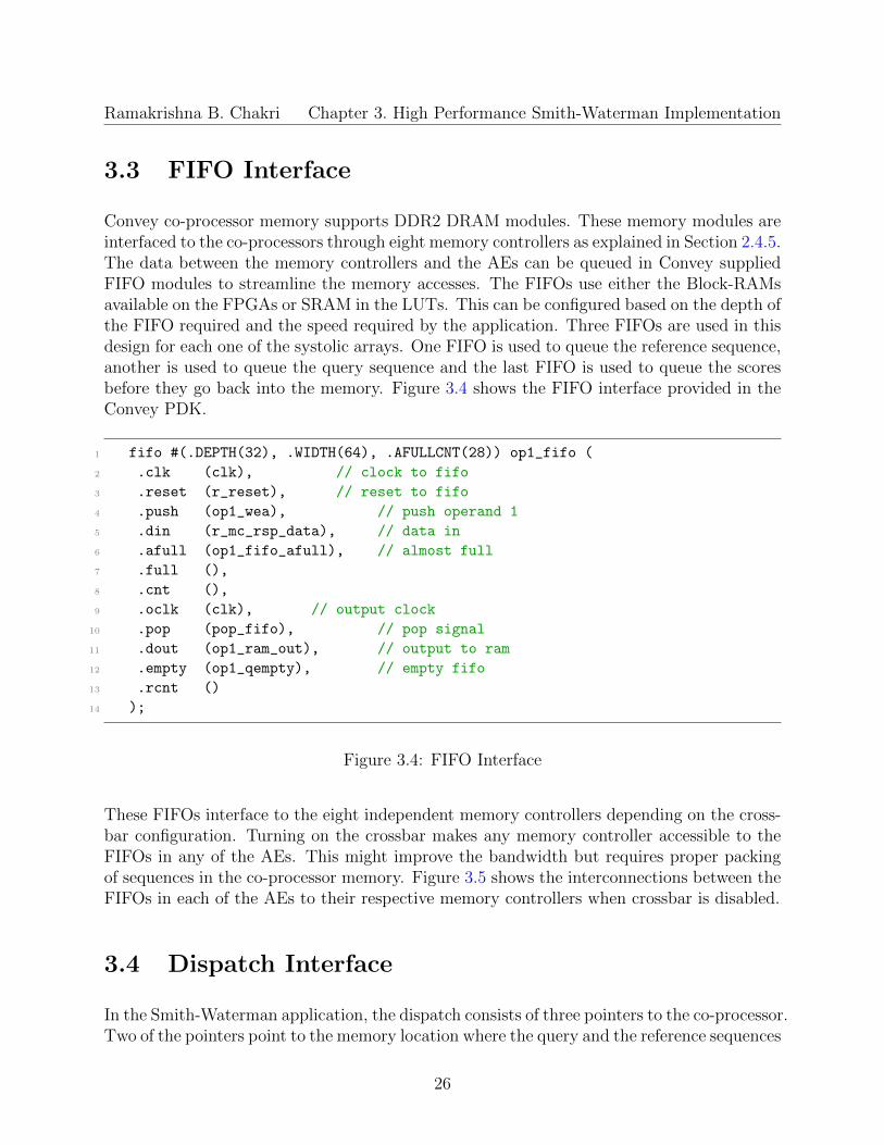
Convey co-processor memory supports DDR2 DRAM modules. These memory modules areinterfaced to the co-processors through eight memory controllers as explained in Section 2.4.5.The data between the memory controllers and the AEs can be queued in Convey suppliedFIFO modules to streamline the memory accesses. The FIFOs use either the Block-RAMsavailable on the FPGAs or SRAM in the LUTs. This can be configured based on the depth ofthe FIFO required and the speed required by the application. Three FIFOs are used in thisdesign for each one of the systolic arrays. One FIFO is used to queue the reference sequence,another is used to queue the query sequence and the last FIFO is used to queue the scoresbefore they go back into the memory. Figure 3.4 shows the FIFO interface provided in theConvey PDK.
1 fifo #(.DEPTH(32), .WIDTH(64), .AFULLCNT(28)) op1_fifo (
2 .clk (clk), // clock to fifo
3 .reset (r_reset), // reset to fifo
4 .push (op1_wea), // push operand 1
5 .din (r_mc_rsp_data), // data in
6 .afull (op1_fifo_afull), // almost full
7 .full (),
8 .cnt (),
9 .oclk (clk), // output clock
10 .pop (pop_fifo), // pop signal
11 .dout (op1_ram_out), // output to ram
12 .empty (op1_qempty), // empty fifo
13 .rcnt ()
14 );
Figure 3.4: FIFO Interface
These FIFOs interface to the eight independent memory controllers depending on the cross-bar configuration. Turning on the crossbar makes any memory controller accessible to theFIFOs in any of the AEs. This might improve the bandwidth but requires proper packingof sequences in the co-processor memory. Figure 3.5 shows the interconnections between theFIFOs in each of the AEs to their respective memory controllers when crossbar is disabled.
3.4 Dispatch Interface
In the Smith-Waterman application, the dispatch consists of three pointers to the co-processor.Two of the pointers point to the memory location where the query and the reference sequences
26

Ramakrishna B. Chakri Chapter 3. High Performance Smith-Waterman Implementation
Memory Controllers
and Modules
x86Host
AE 0
Systolic Arrays
SW Cell SW Cell SW CellSW CellSW Cell SW Cell SW CellSW Cell
SW Cell SW Cell SW CellSW CellSW Cell SW Cell SW CellSW Cell
SW Cell SW Cell SW CellSW CellSW Cell SW Cell SW CellSW Cell
SW Cell SW Cell SW CellSW CellSW Cell SW Cell SW CellSW Cell
SW Cell SW Cell SW CellSW CellSW Cell SW Cell SW CellSW Cell PE Cascade
PE PE PEPE
Refe
renc
e Se
quen
ce
Query Sequence
Scores
AE 2
Systolic Arrays
SW Cell SW Cell SW CellSW CellSW Cell SW Cell SW CellSW Cell
SW Cell SW Cell SW CellSW CellSW Cell SW Cell SW CellSW Cell
SW Cell SW Cell SW CellSW CellSW Cell SW Cell SW CellSW Cell
SW Cell SW Cell SW CellSW CellSW Cell SW Cell SW CellSW Cell
SW Cell SW Cell SW CellSW CellSW Cell SW Cell SW CellSW Cell PE Cascade
PE PE PEPE
Refe
renc
e Se
quen
ce
Query Sequence
Scores
AE 1
Systolic Arrays
SW Cell SW Cell SW CellSW CellSW Cell SW Cell SW CellSW Cell
SW Cell SW Cell SW CellSW CellSW Cell SW Cell SW CellSW Cell
SW Cell SW Cell SW CellSW CellSW Cell SW Cell SW CellSW Cell
SW Cell SW Cell SW CellSW CellSW Cell SW Cell SW CellSW Cell
SW Cell SW Cell SW CellSW CellSW Cell SW Cell SW CellSW CellPE Cascade
PE PE PEPE
Refe
renc
e Se
quen
ce
Query Sequence
Scores
AE 3
Systolic Arrays
SW Cell SW Cell SW CellSW CellSW Cell SW Cell SW CellSW Cell
SW Cell SW Cell SW CellSW CellSW Cell SW Cell SW CellSW Cell
SW Cell SW Cell SW CellSW CellSW Cell SW Cell SW CellSW Cell
SW Cell SW Cell SW CellSW CellSW Cell SW Cell SW CellSW Cell
SW Cell SW Cell SW CellSW CellSW Cell SW Cell SW CellSW Cell PE Cascade
PE PE PEPE
Refe
renc
e Se
quen
ce
Query Sequence
Scores
M1
M1E
M1O
M2
M2E
M2O
M3
M3E
M3O
M5
M5E
M5O
M4
M4E
M4O
M8
M8E
M8O
M6
M6E
M6O
M7
M7E
M7O
Application Engine
Hub(AEH)
Figure 3.5: Final structure of the Smith-Waterman design showing the connections to thememory and the dispatch on Convey HC-1.
are stored in the co-processor memory and the third pointer points to the location in the co-processor memory where the resultant scores are stored. A blocking copcall is made to passthese parameters to the AEs through the dispatch interface. The host processor stalls untilthe AEs complete the execution and returns control to the host. The host application thencopies the scores from co-processor memory and writes it to a file as shown in Figure 5.4.
3.5 Interface to the Bio-applications
In this work, one of the primary goals of the Smith-Waterman application is to provide accel-erated dynamic programming API to any bio-application that has a dynamic programmingphase. Many bio-applications can be partitioned into segments where the dynamic program-ming portion of the application is ported into Convey co-processor through the copcalls,while the rest of the code can reside and execute on the host processor.
27

Ramakrishna B. Chakri Chapter 3. High Performance Smith-Waterman Implementation
3.6 General Purpose-GPUs
The design for Smith-Waterman is implemented in NVIDIA GP-GPUs, GTX 580 and GT440 using the Fermi architecture. This work began with two implementations for computingthe score matrix. One where each thread computes the score for a single cell and the otherwhere each thread computes the score for the an entire row of the Smith-Waterman scorematrix. In both cases the implementation was first done on a global memory and thentransferred to a shared memory location for a faster memory access. CUDA 5.0 was usedfor these implementation.
Since only the maximum scores are tracked, the transfer of the score matrix back and forthbetween host and the GPU is not required and the matrix is used as a scratch pad.
3.6.1 One Thread per Cell
This is a simpler implementation as shown in Figure 3.6 where each thread continuouslyupdates a single cell of the matrix. As each cell is processed by its own thread, the indexingis simpler and there is no change in the index with iterations over a kernel call.
Figure 3.6: One Thread per cell.
However this implementation has an inherit disadvantage that most of the threads are idle.For a m� length query and a n� length reference, the total number of threads required ism ⇤ n while the number of threads in use is limited to the size of the query m. Thus, at anygiven time, (m � 1) ⇤ n threads are idle. The thread requirement also scales quadraticallywith the query and the reference sizes.
3.6.2 One Thread per Row
This is one of the solutions to utilize threads e↵ectively. Here the entire row of cells iscomputed by a single thread. Hence the number of threads launched is equal to the numberof rows which is in turn equal to the query length m. In Figure 3.7, the thread numbercomputing each cell is shown, the thread number is constant across a row as seen.
28

Ramakrishna B. Chakri Chapter 3. High Performance Smith-Waterman Implementation
Figure 3.7: One Thread per Row.
This approach is similar to the Altera’s implementation [25] on a FPGA. This approach hasan index update with each iteration within a kernel. The number of threads are fixed andare equal to the size of the queries. The reference sequences of any size can be used as thenumber of threads does not depend on the size of the reference sequences.
29

Chapter 4
Convey-LabVIEW Interface
This work plays a part in the development of Convey with Virtual Instruments (ConVI)design flow. Here, the LabVIEW programming environment is demonstrated as a viableplatform to build bio-applications on Convey. This work tries to simplify the task of usingheterogeneous systems with re-configurable devices for bioinformatics researchers.
While LabVIEW o↵ers one of the potential design environment for non-hardware designengineers, it is naively supported to only run on National Instruments FPGA targets, calledthe Re-configurable I/O (RIO) devices. It is built to work on embedded platforms and noton data centers. Thus, comes the challenge to interface LabVIEW to high performancesystem such as Convey. The Interactive Front Panel communication on LabVIEW uses apolling-based method of communicating between the Host VI and the FPGA VI by readingand writing indicators and controls [22]. This feature also calls for a robust low latencycommunication channel between the host VI and the FPGA VI.
To accomplish this task, this work builds on the existing work on the Bflow applicationworking on the Azido-Convey interface. Going further, the JTAG interface is exploited toenable the remote access of the application from the LabVIEW front panel.
4.1 LabVIEW FPGA Communication
The LabVIEW front panel communicates with FPGA with constant monitoring of the status,command and data registers in its generated HDL. An Host VI can control and monitor datapassed through the FPGA VI front panel. The values that do not have controls or indicatorscannot be accessed on the wires on the FPGA VI block diagram unless the data is storedin a DMA FIFO. Read/Write Control function reads and writes controls and indicators inthe order they appear in the Read/Write Control function on the block diagram [22]. TheFPGA Module creates a register map, specific to the FPGA VI, that includes a hardware
30
Ramakrishna B. Chakri Chapter 4. Convey-LabVIEW Interface
Figure 4.1: ConVI Overview.
register for every control and indicator.
4.2 Connections and Bit-Mapping
Here, the Convey’s management interface is used to connect the signals to the generatedLabVIEW HDL though a wrapper logic. The CSRs are written through the telnet commandsat the host from the LabVIEW server. The data in CSRs are passed to the LabVIEW HDLthrough its data input ports. The output from the LabVIEW HDL is written to a CSRwhich is retrieved by a CSR read command. This setup is used for run-time communication
31

Ramakrishna B. Chakri Chapter 4. Convey-LabVIEW Interface
Table 4.1: Request and Response formats
Request
Bits : 00� 32 : 4-byte data for the LabVIEW registersBits : 33� 42 : 11-bit Address of the LabVIEW registersBit : 48 : Read StrobeBit : 52 : Write StrobeBits : 56� 57 : 2-bit Message ID
Response
Bits : 00� 32 : 4-byte data for the LabVIEW registersBit : 48 : ReadyBit : 52 : Data ValidBits : 56� 57 : 2-bit Message ID
between Convey and the LabVIEW front panel.
The bit encoding for both CSR and AEG registers, that carry the commands from the MPIPtelnet server to the LabVIEW HDL are shown in Table 4.1 and in Table 4.2.
Here, the Message ID can take four values: 0,1,2,3 and they need to be cycled betweenconsecutive messages to be taken in as a new request. The Message ID for the response willbe the same as the message ID for the request.
4.3 Simulation of ConVI
During simulation, the AEG registers in the dispatch are used in place of CSR for thetransactions due to the lack of interface from the simulator to the management interface.The AEG registers are written through non-blocking copcalls thereby not a↵ecting the hostapplication code running on the x86 processor. Figure 4.2 shows the Convey assemblycode implementing a non-blocking copcall to write and read values from AEG registers thatconnect to the ports of LabVIEW HDL.
4.4 LabVIEW HDL Wrapper
A wrapper is a piece of code that abstracts the use of another piece of code. Wrappers areused to adapt an existing design to have a di↵erent interface. Due to the heterogeneous
32

Ramakrishna B. Chakri Chapter 4. Convey-LabVIEW Interface
1 ##----------------------------------
2 .globl lvload
3 .type lvload. @function
4 .signature pdk=4
5
6 lvload: # function that loads the personality and polls for read/write requests
7 loop:
8 ld.uq $run(%a0),%a20 # Exit the loop if run = 0
9 cmp.uq %a20, %a0, %ac0 # Check for loop complete
10 br %ac0.eq, done # Stop
11
12 ld.uq $mode(%a0),%a22 # load the mode register to decide which action to
be performed
13
14 cmp.uq %a22, $0, %ac0 # 0 for polling back for a different mode
15 br %ac0.eq, loop # Poll
16
17 br loop # stall
18 ##----------------------------------
19 write_lv:
20 ld.uq $Payload_In(%a0),%a30 # load the payload into a30
21 mov.ae0 %a30,$0,%aeg # move the payload into aeg0 to dataport in
22 st.uq %a0, $mode(%a0) # change mode back to 0 for polling
23 br loop # stall and wait for next request
24
25 read_lv:
26 mov.ae0 %aeg,$0,%a30 # read the dataport out through aeg0
27 st.uq %a30,$Data_Out(%a0) # store the value into Data out
28 st.uq %a0, $mode(%a0) # change mode back to 0 for polling
29 br loop # stall and wait for next request
30 ##----------------------------------
31 done:
32 rtn
33
34 lvloadEnd:
35 .globl lvload
36 .type lvload. @function
37 .cend
38 ##----------------------------------
Figure 4.2: Non-blocking copcall in Convey assembly code
33

Ramakrishna B. Chakri Chapter 4. Convey-LabVIEW Interface
Table 4.2: The Bit Mapping for LabVIEW Commands through 64-bit CSR and AEG Reg-isters.
64 bits of the CSR/AEG registers CSR 0x8007 CSR 0x8008 Mask
7 6 5 4 3 2 1 0 Data-LSB Data-LSB FF15 14 13 12 11 10 9 8 Data-LSB Data-LSB FF23 22 21 20 19 18 17 16 Data-MSB Data-MSB FF31 30 29 28 27 26 25 24 Data-MSB Data-MSB FF39 38 37 36 35 34 33 32 Address-LSB X/X FF47 46 45 44 43 42 41 40 X/Address-MSB X/X 0755 54 53 52 51 50 49 48 Write/Read Valid/Ready 1163 62 61 60 59 58 57 56 X/Msg-ID X/ Msg-ID 03
nature of Convey, LabVIEW does not have a built-in support to interface the peripheralsof the Convey computers. Hence, a wrapper is used to interface the LabVIEW generatedHDL to Convey’s top-level HDL called cae pers. Figure 4.3 gives the block diagram of thewrapper. The wrapper serves the purpose of interfacing the HDL generated from LabVIEWto the Convey environment. The LV HDL has three input ports, and three output ports.Each of the three pairs of input/output ports are used to interface to the memory, dispatchand the management interfaces. As shown in Figure 4.3, the wrapper consists of these parts:
1. A stub to connect to all the I/O ports coming out of LabVIEW HDL that connects tothe originally intended Spartan-3E board: This stub simulates the environment of theSpartan-3E board for the LabVIEW HDL.
2. An interface to the streamer source and sink HDLs to stream data in and out of theco-processor memory: The input port interfaces with the source streamer that streamsthe data from the co-processor memory into FPGAs, which in turn is streamed to theLV HDL block. This interface is used to fetch the sequences from memory. The outputport interfaces with the sink streamer which streams the alignment scores generatedin the LV HDL to the co-processor memory.
3. Interface to the AEG registers through the I/O in the modified XML resource file:These are used to interface the LV HDL to the dispatch interface. These are used totransfer data from the host application to the LV HDL. In this application, the inputdata can be a pointer to the memory location where the sequences are stored.
4. Interface to the BPORT IN and BPORT OUT ports, which are the interfaces to theLabVIEW HDL from the VI Front panel: These are interfaced to the managementprocessor. Here the input port is used to send the commands to read/write the registers
34
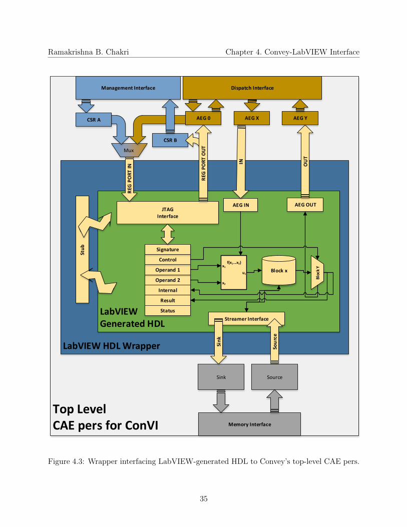
Ramakrishna B. Chakri Chapter 4. Convey-LabVIEW Interface
Top LevelCAE pers for ConVI
LabVIEW HDL Wrapper
LabVIEW Generated HDL
Operand 2
Internal
Result
Operand 1
Control
Signature
Status
JTAGInterface
u1
x2
x1f(x1...x2)
Bloc
k Y
AEG IN AEG OUT
Block x
Streamer Interface
Sour
ce
Stub
Memory Interface
Dispatch InterfaceManagement Interface
Sink Source
Sink
OU
T
REG
PO
RT IN
Mux
CSR B
AEG YAEG X
REG
PO
RT O
UT
AEG 0CSR A
Figure 4.3: Wrapper interfacing LabVIEW-generated HDL to Convey’s top-level CAE pers.
35

Ramakrishna B. Chakri Chapter 4. Convey-LabVIEW Interface
from the LabVIEW front panel and an output port is used to send the data back tothe front panel as explained in Section 4.2.
4.5 Designing using LabVIEW
After designing the LabVIEW-Convey communication channel and the wrapper, LabVIEWis used for designing applications for the hardware accelerator. To demonstrate this designflow using LabVIEW, a 16-PE Smith-Waterman pipeline is designed in LabVIEW. First,a single PE of Smith-Waterman is designed using the LabVIEW graphical programminglanguage as shown in Figure 4.4. This PE is replicated using LabVIEW VI scripting [44] togenerate a 16-PE pipeline as shown in Figure 4.5. Running this application generates theHDLs for this design, which are copied to a directory with other files from Convey PDKfor simulation and synthesis using Convey tools. This design runs on the Convey HC-1accelerator and communicates with the LabVIEW front panel thereby providing the user tocontrol and monitor the accelerator using the LAbVIEW’s graphical interface as shown inFigure 4.6. Thus, the complex job of designing the accelerator for Convey HC-1 is simplifiedby using LabVIEW.
Figure 4.4: Smith-Waterman PE designed using LabVIEW.
36

Ramakrishna B. Chakri Chapter 4. Convey-LabVIEW Interface
Figure 4.5: A 16-PE pipeline generated using LabVIEW VI Scripting.
Figure 4.6: LabVIEW front panel with controls and indicators for Smith-Waterman appli-cation running on Convey HC-1.
37

Chapter 5
Results and Analysis
This chapter focuses on the results of the high performance Smith-Waterman implemen-tations and the implementation of LabVIEW’s interface to Convey HC-1. This chapter isdivided into the following sections. The first and the second sections deal with the results ofthe high performance Smith-Waterman on Convey HC-1 and NVIDIA GP-GPU respectively.Then the performance of these implementations are compared with the recent work done inthis area. Finally, the results of the LabVIEW based interface to Convey, called ConVI, isdiscussed.
5.1 High Performance Smith-Waterman
The Smith-Waterman algorithm was designed for the Convey HC-1 accelerator with a singleSmith-Waterman PE first, then the design was cascaded into a pipeline to form a com-plete systolic array. The pipelines were replicated as much as possible to take the completeadvantage of the available logic resources and the memory bandwidth in the system.
As the number of PEs in a FPGA directly translates to the performance, emphasis here isto maximize the number of PEs contained in each of the AEs. Hence, the Section 5.1.1 dealswith the area and resources in the fabric used for building the accelerator. The amount ofdata consumed per cycle by the application engines is directly proportional to the numberof PEs in the design; thus, a theoretical estimate of the bandwidth is presented in the Sec-tion 5.1.2. Finally, this design is tested by simulating it using the Convey’s HDL simulator.The waveforms in the timing diagram are analyzed using the Synopsys DVE tool to verifythe assumptions. These are reported in the Section 5.1.3.
38
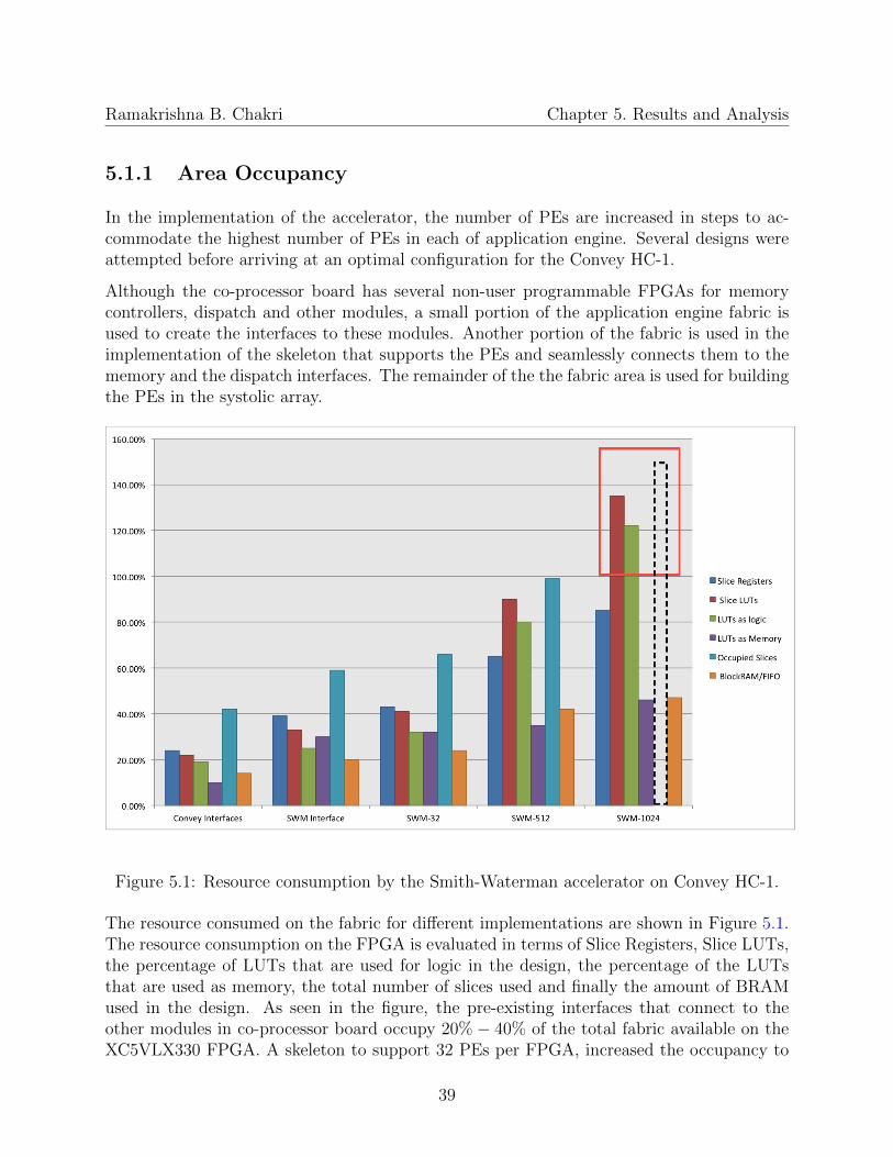
Ramakrishna B. Chakri Chapter 5. Results and Analysis
5.1.1 Area Occupancy
In the implementation of the accelerator, the number of PEs are increased in steps to ac-commodate the highest number of PEs in each of application engine. Several designs wereattempted before arriving at an optimal configuration for the Convey HC-1.
Although the co-processor board has several non-user programmable FPGAs for memorycontrollers, dispatch and other modules, a small portion of the application engine fabric isused to create the interfaces to these modules. Another portion of the fabric is used in theimplementation of the skeleton that supports the PEs and seamlessly connects them to thememory and the dispatch interfaces. The remainder of the the fabric area is used for buildingthe PEs in the systolic array.
Figure 5.1: Resource consumption by the Smith-Waterman accelerator on Convey HC-1.
The resource consumed on the fabric for di↵erent implementations are shown in Figure 5.1.The resource consumption on the FPGA is evaluated in terms of Slice Registers, Slice LUTs,the percentage of LUTs that are used for logic in the design, the percentage of the LUTsthat are used as memory, the total number of slices used and finally the amount of BRAMused in the design. As seen in the figure, the pre-existing interfaces that connect to theother modules in co-processor board occupy 20% � 40% of the total fabric available on theXC5VLX330 FPGA. A skeleton to support 32 PEs per FPGA, increased the occupancy to
39

Ramakrishna B. Chakri Chapter 5. Results and Analysis
40%� 60%. This design was populated with 32 PEs to increase the occupancy by 5%� 10%greater than the existing skeleton. This structure was replicated in the design until it couldsupport 512 PEs per AE with an occupancy of 80%� 99%.
This implementation involved a pipeline with 32 processing elements, and 16 pipelines perAE, giving rise to 16 ⇤ 4 ⇤ 32 = 2048 processing elements to achieve a peak theoreticalthroughput of 2048 PE * 150 MHz = 307 GCUPS (Giga Cell Updates per Second). Thesynthesis report of this design on the AEs is attached below. The report shows that this isa proper fit for the XC5VLX330 FPGA.
1 Release 14.1 Map P.15xf (lin64)
2 Xilinx Mapping Report File for Design ’cae_fpga’
3
4 Design Information
5 ------------------
6 Command Line : map -intstyle xflow -pr b -detail -ignore_keep_hierarchy -xe n
-w -t 1 -ol high -o cae_fpga.ncd
7 cae_fpga.ngd
8 Target Device : xc5vlx330
9 Target Package : ff1760
10 Target Speed : -2
11 Mapper Version : virtex5 -- $Revision: 1.55 $
12 Mapped Date : Wed Apr 17 19:28:48 2013
13
14 Design Summary
15 --------------
16 Number of errors: 0
17 Number of warnings: 425
18 Slice Logic Utilization:
19 Number of Slice Registers: 136,336 out of 207,360 65%
20 Number used as Flip Flops: 135,792
21 Number used as Latches: 544
22 Number of Slice LUTs: 187,057 out of 207,360 90%
23 Number used as logic: 166,244 out of 207,360 80%
24 Number using O6 output only: 127,283
25 Number using O5 output only: 5,744
26 Number using O5 and O6: 33,217
27 Number used as Memory: 19,578 out of 54,720 35%
28 Number used as Dual Port RAM: 19,290
29 Number using O6 output only: 2,098
30 Number using O5 output only: 1,153
31 Number using O5 and O6: 16,039
32 Number used as Shift Register: 288
33 Number using O5 and O6: 288
34 Number used as exclusive route-thru: 1,235
40

Ramakrishna B. Chakri Chapter 5. Results and Analysis
35 Number of route-thrus: 7,307
36 Number using O6 output only: 6,866
37 Number using O5 output only: 328
38 Number using O5 and O6: 113
39
40 Slice Logic Distribution:
41 Number of occupied Slices: 51,652 out of 51,840 99%
42 Number of LUT Flip Flop pairs used: 200,442
43 Number with an unused Flip Flop: 64,106 out of 200,442 31%
44 Number with an unused LUT: 13,385 out of 200,442 6%
45 Number of fully used LUT-FF pairs: 122,951 out of 200,442 61%
46 Number of unique control sets: 4,732
47 Number of slice register sites lost
48 to control set restrictions: 8,591 out of 207,360 4%
49
50 A LUT Flip Flop pair for this architecture represents one LUT paired with
51 one Flip Flop within a slice. A control set is a unique combination of
52 clock, reset, set, and enable signals for a registered element.
53 The Slice Logic Distribution report is not meaningful if the design is
54 over-mapped for a non-slice resource or if Placement fails.
55 OVERMAPPING of BRAM resources should be ignored if the design is
56 over-mapped for a non-BRAM resource or if placement fails.
57
58 IO Utilization:
59 Number of bonded IOBs: 861 out of 1,200 71%
60 Number of LOCed IOBs: 861 out of 861 100%
61 IOB Flip Flops: 1,016
62 IOB Master Pads: 20
63 IOB Slave Pads: 20
64
65 Specific Feature Utilization:
66 Number of BlockRAM/FIFO: 122 out of 288 42%
67 Number using BlockRAM only: 122
68 Total primitives used:
69 Number of 36k BlockRAM used: 97
70 Number of 18k BlockRAM used: 33
71 Total Memory used (KB): 4,086 out of 10,368 39%
72 Number of BUFG/BUFGCTRLs: 26 out of 32 81%
73 Number used as BUFGs: 2
74 Number used as BUFGCTRLs: 24
75 Number of IDELAYCTRLs: 18 out of 34 52%
76 Number of DCM_ADVs: 1 out of 12 8%
77 Number of LOCed DCM_ADVs: 1 out of 1 100%
78 Number of ISERDESs: 356
79 Number of OSERDESs: 20
41

Ramakrishna B. Chakri Chapter 5. Results and Analysis
80 Number of PLL_ADVs: 2 out of 6 33%
81 Number of LOCed PLL_ADVs: 2 out of 2 100%
82 Number of SYSMONs: 1 out of 1 100%
83
84 Number of RPM macros: 72
85 Average Fanout of Non-Clock Nets: 3.65
86
87 Peak Memory Usage: 5857 MB
88 Total REAL time to MAP completion: 3 hrs 25 mins 30 secs
89 Total CPU time to MAP completion: 3 hrs 24 mins 33 secs
Figure 5.2: Resource allocation for each of the components in the design.
Figure 5.2 shows the allocation of resources for each of those components in the optimumdesign for HC-1 with 512 PEs per AE. It can be seen that the major chunk of the fabric isoccupied by the 512 PEs. Most of the LUTs (55%) are used to implement logic functionsand few of them (5%) are used for memory in the PE designs while the opposite is true inthe case of the systolic array skeleton. The Convey-provided interface has up to 40% of usedslices as seen before.
Figure 5.1 also shows a final implementation with 1024 PEs per FPGA. This attempt involveda pipeline with 64 processing elements, and 16 pipelines per AE, giving rise to 16⇤4⇤64 = 4096processing elements to achieve a peak theoretical throughput of 4096 PE * 150 MHz = 614
42

Ramakrishna B. Chakri Chapter 5. Results and Analysis
GCUPS (Giga Cell Updates per Second). The red box in the figure indicates that the designgoes out of bounds for the XC5VLX330 FPGA. However this design can be used to programthe Convey HC-1ex platform, since it contains the XC6VLX760 FPGA, which has more thantwice the number of resources as the XC5VLX330 [45].
5.1.2 Bandwidth Requirements
As both HC-1 and the HC-1ex have the same memory bandwidth capacity, both the plat-forms have the same calculation.
InputsEach PE requires 4 bits from memory: 2 for query and 2 for database.Each PE requires a single byte character from the block RAM for scoring.Each PE requires a 2-byte short integer max score and five scores for computation.
OutputsEach PE sends out a 3-bit direction vector to memory.Each PE sends out its own value.
AssumptionsEach PE update is done in one clock cycle.The design runs at maximum clock speed of 150 MHz.The entire query sequence resides on the FPGA after a initial phase.With striding enabled, the peak bandwidth available = 20 GB/sec [1].Aggregate bandwidth for 4 AEs = 640 Gigabits/sec.
AE-Memory bandwidth required without trace-backNumber of bits per cycle per AE = 4 bits.Number of bits for all the 4 AEs = 16 bits.Therefore bandwidth required = 150 ⇤ 106 ⇤ 16 = 2.4 Gigabits/sec.This fits well within the maximum supported bandwidth.
Bandwidth required to store the trace-back vectorsNumber of bits to send the directions information per cell = 3 bits.Bandwidth required for Trace-back Vectors = 150 ⇤ 106 ⇤ 3 ⇤ 2048 = 921.6 Gigabits/sec.This is a high value to be practically incorporated on Convey HC systems.Hence, trace-back is not used.
Thus, this is a compute-bound problem in Convey when trace-back is not performed inhardware. With trace-back, memory bandwidth becomes the bottleneck in the system.
43

Ramakrishna B. Chakri Chapter 5. Results and Analysis
Figure 5.3: Timing diagram showing the alignment score calculations.
44

Ramakrishna B. Chakri Chapter 5. Results and Analysis
Figure 5.4: The output of the accelerator: the sequence numbers with the scores of theirpairwise alignment.
5.1.3 Simulation
The designs were simulated on Convey HDL simulator using the Synopsys tools. Figure 5.3shows the timing diagram for the resultant scores being stored back to the memory. Everyspike in the lower part of the diagram represents the availability at the compute cores andthe start of an alignment. The steady and continuous flow of data and availability of results,represents a streamlined memory access. Thus, the assumptions made in the previous sectionare verified here.
Figure 5.4 shows the resultant scores generated from the simulation of 2000 sequences againstanother 2000 sequences. Each systolic array in the accelerator finds the pairwise alignmentscores between two sequences and stores the scores in order in the co-processor memory.The scores were read from the co-processor memory and printed on to a file. These scoreswere verified from a software implementation and was tested for 100% accuracy in the valuesobtained.
5.2 Performance with GP-GPU
The GP-GPU programs were executed on two di↵erent devices, the NVIDIA GeForce GTX580 and the NVIDIA GeForce GT 440. Both of these units are based on the NVIDIA FermiArchitecture [46]. However, some of the di↵erences between them is highlighted in Table 5.1.Analysis were performed on the time taken for the program execution. The results and theiranalysis is discussed below.
The speedup is calculated by comparing the parallel version of the program on GPU over theserial version of the program running on a x86 processor with the following specifications:
45

Ramakrishna B. Chakri Chapter 5. Results and Analysis
Table 5.1: Key features of the platforms usedFeatures GT440 GTX580
CUDA Capability 2.1 2.0Total no of MPs 3 16CUDA Cores/MP 48 32GPU Clock Rate 1189 MHz 1544 MHz
Shared Memory per Block 49152 bytes 49152 bytesMax Threads per Multiprocessor 1536 1536
Max Threads per Block 1024 bytes 1024Registers Per Block 32768 32768
Model name : Intel(R) Core(TM) i7 CPUCPU frequency : 960 @ 3.20GHzCache size : 8192 KB
The parallel version of the program was executed on GTX580 and Figure 5.5 shows the
Figure 5.5: Kernel speedup with number of target and search sequences over x86.
raw kernel speedup attained with various query and reference database sizes over the serial
46

Ramakrishna B. Chakri Chapter 5. Results and Analysis
x86 processor. Speedup of up to 4500x were observed as seen in Figure 5.5. The overhead of
Figure 5.6: Overall speedup attained by using the GP-GPU over x86 processor.
transferring the data back and forth between the host and the device memory and the over-head of memory allocations on the GPU were considered while analyzing the overall tradeo↵ of using GPU parallel application. The graph plotted is seen in Figure 5.6. Speedupof up to 1100x have been attained for specific configurations of query and database sizes.This is partly due to the fact that in this approach, the score matrix is not involved in thememory copy overhead.
47

Ramakrishna B. Chakri Chapter 5. Results and Analysis
5.3 Performance Compared With Recent Work
This section compares the Smith-Waterman implemented in this work with some of theother recent contributions discussed in Section 2.7. The Table 5.2 compares the maximumthroughput in GCUPS that can be attained with these implementations. Of the total sixteenimplementations, seven of them are based on GP-GPUs, eight of them are based on FPGAsand one of them on Cell Broadband Engine. Of the seven GP-GPU based implementations,two of them are dual GPUs on a single graphics card.
Figure 5.7 shows the plot of these values on a bar chart. Logarithmic scale is used toaccommodate the large scale ranging from 3.5 GCUPS on GeForce 8800 GP-GPU to 768GCUPS in Convey HC-1ex with four Virtex-6 FPGAs. The red colored bars indicates theimplementations from this work. It can be seen that Convey’s implementation of theirapplication cnysws comes close in performance to the Smith-Waterman implemented in thiswork. The graph however is dominated by the Convey’s cnysws on HC-1ex with a throughputof 768 GCUPS followed by two other implementations on HC-1. The performance in theGTX 580 falls short of the other GP-GPU implementation, due to the lack of any changesto the native algorithm.
Table 5.2: Performance comparison with related work on heterogeneous computers.Name Platform Peak Performance (GCUPS)
Issac et al. [32] Altera Stratix EP1S40 23.8Wirawan et al. [40] Cell-Broadband Engine (BE) 3.6
Convey [3] Convey HC-1 259This Work Convey HC-1 307.2Convey [3] Convey HC-1ex 768
CUDA++ [36] NVIDIA GTX 295 (dual) 16.087CUDA++3.0 [34] NVIDIA GTX690 (dual) 185.6Svetlin et al. [35] NVIDIA GeForce 8800 GTX 3.5
This Work NVIDIA GTX 580 9.98CUDA Align 2.0 [38] NVIDIA GTX285 23
CUDA++ [36] NVIDIA GTX 280 9.66CUDA++2.0 [15] NVIDIA GTX 280 17CUDA++3.0 [34] NVIDIA GTX680 119
Altera white paper [25] XtremeData XD1000 25.6Allred et al. [33] XtremeData IXD2000i 9.0Oliver et al. [31] Xilinx XC2V6000 5.0
48

Ramakrishna B. Chakri Chapter 5. Results and Analysis
Figure 5.7: Throughput comparison of recent work on high performance Smith-Water Im-plementation.
5.4 LabVIEW Convey Interface
The LabVIEW Convey interface was successfully deployed with the ConVI design flow. Awrapper was built around the LabVIEW generated HDL, it was interfaced to the AEGregisters and streamers successfully. The BPORT IN and the BPORT OUT were connectedto the CSR and AEG registers. The updates from the VI front panel controls are passedthrough the ConVI execution server to the CSR/AEG resisters to update the values withinthe LabVIEW HDL. The values of the indicators were transferred from the LV HDL to thefront panel.
ConVI as a design flow and LabVIEW as a HDL design tool was put to test during the VBI-NSF workshop. A team of five participants from di↵erent backgrounds were provided witha half-day training on NI LabVIEW. The team was provided with a basic Smith-WatermanLabVIEW implementation and was asked to make modifications to the design. The teamwas able to successfully come up with the modifications without any detailed knowledge ofConvey PDK or HDL experience. Finally, the use of this tool for accelerator developmentreceived a positive response from the team.
49

Ramakrishna B. Chakri Chapter 5. Results and Analysis
The following subsections compare ConVI to other high level programming paradigms dis-cussed in Section 2.7.
5.4.1 Comparing ConVI with Bflow
Design Environment: LabVIEW was primarily made for Virtual Instruments while Azidowas specific to HDL design on Xilinx FPGA. Although Azido seems to have an advantagehere, the LabVIEW design environment is more mature and stable and has a library ofmodules specially designed for FPGA implementations.
Design Files: ConVI runs on LabVIEW generated HDL while Bflow runs on Azido gener-ated EDIF files. HDL files have the advantage where the source can be analyzed and can bemodified. Wrappers can be easily designed for HDL files. EDIF files are netlists and theycannot be modified and does not have the flexibility that is present in HDL source files.
Interface Objects: Bflow connects to the hardware through COM objects while LabVIEWgenerates registers in hardware for every control and indicator. LabVIEW again has theadvantage here since the register interface is independent of the design. This makes it easierto design the wrappers for the design as the interface is left unchanged and the LabVIEWcommunicates directly with the registers.
5.4.2 Comparison with OpenCL Smith-Waterman
OpenCL is another high level programming model that is used to program the di↵erent typesof processors in an heterogeneous computer in a single programming paradigm. OpenCLwas initially developed by Apple inc to support general purpose computing on GPUs acrossdi↵erent vendors. This was later being extended to other platforms. Although OpenCL is aproven solution to program heterogeneous systems, the programmer still requires skill setsin parallel programming and must be architecture aware to deploy an application e↵ectively.
LabVIEW o↵ers the advantages of visualizing the modules and the parallelism in the al-gorithm. Architecture independent programming, real time monitoring and the ability togenerate C code, places LabVIEW above OpenCL programming paradigm for FPGAs andFPGA based heterogeneous systems.
50

Chapter 6
Conclusion and Future Scope
This work demonstrated some of the ways of enabling the use of heterogeneous systems forbio-informatics applications. Here is an abridgment of the contributions from this work.
1. An e�cient implementation of dynamic programming based Smith-Waterman wasachieved. This work aimed to accelerate bio-applications by e�cient usage of het-erogeneous systems. The performance in GCUPS attained is higher than Convey’spersonality on HC-1.
2. A similar approach was used to implement Smith-Waterman on NVIDIA GP-GPUsusing CUDA. This was compared to the performance of Smith-Waterman on ConveyHC-1 and other GP-GPU/FPGA based systems.
3. The design of accelerator using LabVIEW was demonstrated. This proved to be ahighly viable option to design and control the accelerator without of the domain knowl-edge and HDL skills. The ultimate aim of this work is to enable the bioinformaticiansto be able to work free of hardware design engineers.
There is however many potential enhancements that can be incorporated in the future. Thenext three sections discusses the scope for future improvements in each of the tasks performedin this work.
6.1 Dynamic Programming Environment on Convey
With a dynamic programming personality being setup in Convey, one may use it for a widevariety of applications that have dynamic programming phase in them. BFAST and BWASWare the examples of two algorithms that accelerates the native Smith-Waterman. BFASTuses indexes to filter seeds while BWASW uses BWT to filter the number of alignment
51

Ramakrishna B. Chakri Chapter 6. Conclusion and Future Scope
locations. Following is the description of the di↵erent phases of these two algorithms andhow the Smith-Waterman hardware implementation can be incorporated. A similar approachcan be followed for any algorithm with a Smith-Waterman phase in it.
6.1.1 Burrows-Wheeler Aligner Smith-Waterman (BWASW)
BWASW [5] involves the use of Burrows Wheelers Transform [47] to pre-process the genomesequences. A prefix tree is built from the reference sequence and a Prefix Dynamic AcyclicWord Graph (DAWG) is formed from the query sequence. The prefix DAWG is parsedover the prefix tree to find the alignment locations. The seeds are expanded using theSmith-Waterman algorithm making it suitable for long reads up to 100,000 base pair fromRoche/454 sequencing technologies. The following are the steps in this algorithm,
1. Formation of Prefix trie of the reference sequence.
2. Formation of the Prefix-DAWG of the query sequence.
3. Aligning Prefix trie against Prefix DAWG.
4. Acceleration by the standard Smith-Waterman algorithm.
Figure 6.1: Proposed BWA-SW on Convey HC systems.
Figure 6.1 shows the proposed implementation of BWASW on Convey HC-1. As seen in thefigure, the Hardware Align phase consists of Smith-Waterman which can be e�ciently accel-erated in the FPGA. The dotted line indicates a further enhancement to the applications.Depending on the load distribution, BWT phase can also be mapped to hardware [48] tooptimize the performance.
52

Ramakrishna B. Chakri Chapter 6. Conclusion and Future Scope
6.1.2 BLAT like Fast and Accurate Search Tool (BFAST)
BFAST [7] aims to attain more accuracy by employing Smith-Waterman expansion. BFASTpre-computes an index of all non overlapping k-mers in the genome. This index fits inside theRAM of inexpensive computers, and need only be computed once for each genome assembly.It supports both Illumina and ABI’s SOLiD reads. The following are the steps followed byBFAST,
1. Preprocessing the reference sequence.
2. Indexing process for the reference genome.
3. Matching the query with the indexed reference genome.
4. Local alignment using the Smith-Waterman algorithm.
5. Post processing and performing the alignments.
Figure 6.2: Proposed BFAST on Convey HC systems.
Figure 6.2 shows the proposed implementation of BFAST on Convey. The Align stage ofBFAST can benefit from this Smith-Waterman implementation in the hardware. Dependingon the parameters used, the match phase can be time consuming and would benefit fromo✏oading it to hardware as demonstrated by Corey et al. [28].
6.2 Dynamic Parallelism using Kepler GP-GPUs
Dynamic Parallelism in CUDA is supported via an extension to the CUDA programmingmodel that enables a CUDA kernel to create and synchronize new nested work [49]. Basically,
53

a child CUDA kernel can be called from within a parent CUDA kernel and then optionallysynchronize on the completion of that child CUDA kernel. The parent CUDA kernel canconsume the output produced from the child CUDA kernel, all without the CPU involvement.Use of dynamic parallelism in Kepler architecture can further eliminate use of more threadsby dynamically making decisions for launching threads within a kernel call. This would alsoenable the reuse of the scoring matrix.
6.3 Unified Programming with LabVIEW for Convey
Apart from the HDL generating capabilities of LabVIEW, it can create a C code thatrepresents the algorithm developed graphically in LabVIEW [50]. With the LabVIEW CGenerator, no target knowledge is required because the software generates ANSI C codefrom a LabVIEW application instead of generating target-specific binary code. This canbe used to the advantage in generating the host code for Convey along with the hardwaredesign. This enables the unification of the development platforms for both host and theFPGAs in Convey HC-1. Thus, LabVIEW has a great potential to be the development toolfor programming heterogeneous platforms.

Bibliography
[1] Convey HC Reference Manual. Convey Computer, 2012.
[2] Convey Personality Development Kit Reference Manual. Convey Computer, 2012.
[3] Smith-Waterman Datasheet. Convey Computer, 2011.
[4] S. B. Needleman and C. D. Wunsch, “A general method applicable to thesearch for similarities in the amino acid sequence of two proteins,” Journal ofMolecular Biology, vol. 48, no. 3, pp. 443 – 453, 1970. [Online]. Available:http://www.sciencedirect.com/science/article/pii/0022283670900574
[5] H. Li and R. Durbin, “Fast and accurate long-read alignment with Burrows Wheelertransform,” vol. 26, no. 5, pp. 589–595, 2010.
[6] P. Gupta, “Swift: A GPU-based Smith-Waterman Sequence Alignment Program,” May2012.
[7] N. Homer, B. Merriman, and S. F. Nelson, “BFAST: an alignment toolfor large scale genome resequencing.” PloS one, vol. 4, no. 11, p. e7767, Jan.2009. [Online]. Available: http://www.pubmedcentral.nih.gov/articlerender.fcgi?artid=2770639&tool=pmcentrez&rendertype=abstract
[8] “Isolating, Cloning, and Sequencing DNA,” 2002. [Online]. Available: http://www.ncbi.nlm.nih.gov/books/NBK26837/
[9] H. Li and R. Durbin, “Fast and accurate short read alignment with Burrows Wheelertransform,” vol. 25, no. 14, pp. 1754–1760, 2009.
[10] D. W. Mount, Bioinformatics: Sequence and Genome Analysis, 2nd ed. Cold SpringHarbor Press, 2004.
[11] A. Khalafallah, H. Elbabb, O. Mahmoud, and A. Elshamy, “Optimizing smith-watermanalgorithm on graphics processing unit,” in Computer Technology and Development (IC-CTD), 2010 2nd International Conference on, 2010, pp. 650–654.
55

[12] S. Arming, R. Fenkhuber, and T. Handl, “Data Compression in Hardware The Burrows-Wheeler Approach,” pp. 60–65, 2010.
[13] P. Ferragina and G. Manzini, “Opportunistic data structures with applications,” inProceedings of the 41st Annual Symposium on Foundations of Computer Science, ser.FOCS ’00. Washington, DC, USA: IEEE Computer Society, 2000, pp. 390–. [Online].Available: http://dl.acm.org/citation.cfm?id=795666.796543
[14] R. A. Baeza-Yates and G. H. Gonnet, “Fast text searching for regular expressionsor automaton searching on tries,” J. ACM, vol. 43, no. 6, pp. 915–936, Nov. 1996.[Online]. Available: http://doi.acm.org/10.1145/235809.235810
[15] Y. Liu, B. Schmidt, and D. Maskell, “Cudasw++2.0: enhanced smith-watermanprotein database search on cuda-enabled gpus based on simt and virtualized simdabstractions,” BMC Research Notes, vol. 3, no. 1, p. 93, 2010. [Online]. Available:http://www.biomedcentral.com/1756-0500/3/93
[16] T. Smith and M. Waterman, “Identification of common molecular subsequences,”Journal of Molecular Biology, vol. 147, no. 1, pp. 195 – 197, 1981. [Online]. Available:http://www.sciencedirect.com/science/article/pii/0022283681900875
[17] “FPGAs,” http://www.altera.com/products/fpga.html.
[18] Virtex-5 Family Overview. Xilinx, february 2009.
[19] D. Uliana, K. Kepa, and P. Athanas, “Fpga-based hpc application design for non-experts (abstract only),” in Proceedings of the ACM/SIGDA international symposiumon Field programmable gate arrays, ser. FPGA ’13. New York, NY, USA: ACM, 2013,pp. 274–274. [Online]. Available: http://doi.acm.org/10.1145/2435264.2435334
[20] Z. Jin and J. D. Bakos, “Extending the BEAGLE library to a multi-FPGAplatform.” BMC bioinformatics, vol. 14, no. 1, p. 25, Jan. 2013. [Online]. Available:http://www.biomedcentral.com/1471-2105/14/25
[21] Convey Coprocessor Memory Ordering. Convey Computer, january 2012.[Online]. Available: http://www.conveysupport.com/alldocs/WhitePapers/PDK/WP Coprocessor Memory Order.pdf
[22] LabVIEW 2012 FPGA Module Help. National Instruments.
[23] D. Kirk and W. Hwu, Programming Massively Parallel Processors: A Hands-on Ap-proach, 1st ed. Morgan Kaufmann, 2010.
[24] NVIDIA CUDA Programming Guide 2.0. NVIDIA, 2008.
[25] “Implementation of the smith-waterman algorithm on a reconfigurable supercomputingplatform,” ALTERA Whitepaper, 2007.

[26] Y. Chen, B. Schmidt, and D. L. Maskell, “Accelerating short read mapping on an fpga(abstract only),” in Proceedings of the ACM/SIGDA international symposium on FieldProgrammable Gate Arrays, ser. FPGA ’12. New York, NY, USA: ACM, 2012, pp.265–265. [Online]. Available: http://doi.acm.org/10.1145/2145694.2145740
[27] E. Fernandez, W. Najjar, and S. Lonardi, “String matching in hardware using thefm-index,” in Proceedings of the 2011 IEEE 19th Annual International Symposiumon Field-Programmable Custom Computing Machines, ser. FCCM ’11. Washington,DC, USA: IEEE Computer Society, 2011, pp. 218–225. [Online]. Available:http://dx.doi.org/10.1109/FCCM.2011.55
[28] C. B. Olson, M. Kim, C. Clauson, B. Kogon, C. Ebeling, S. Hauck, and W. L. Ruzzo,“Hardware Acceleration of Short Read Mapping,” 2012 IEEE 20th InternationalSymposium on Field-Programmable Custom Computing Machines, pp. 161–168,Apr. 2012. [Online]. Available: http://ieeexplore.ieee.org/lpdocs/epic03/wrapper.htm?arnumber=6239809
[29] S. I. Steinfadt, “SWAMP+: Enhanced Smith-Waterman Search for Parallel Models,”in 2012 41st International Conference on Parallel Processing Workshops. IEEE,Sep. 2012, pp. 62–70. [Online]. Available: http://ieeexplore.ieee.org/lpdocs/epic03/wrapper.htm?arnumber=6337464
[30] G. Chrysos, E. Sotiriades, C. Rousopoulos, A. Dollas, A. Papadopoulos, I. Kirmitzoglou,V. Promponas, T. Theocharides, G. Petihakis, J. Lagnel, P. Vavylis, and G. Kotoulas,“Opportunities from the use of fpgas as platforms for bioinformatics algorithms,” inBioinformatics Bioengineering (BIBE), 2012 IEEE 12th International Conference on,2012, pp. 559–565.
[31] T. Oliver, B. Schmidt, and D. Maskell, “Reconfigurable architectures for bio-sequencedatabase scanning on FPGAs,” IEEE Transactions on Circuits and Systems II:Express Briefs, vol. 52, no. 12, pp. 851–855, Dec. 2005. [Online]. Available:http://ieeexplore.ieee.org/lpdocs/epic03/wrapper.htm?arnumber=1556805
[32] I. T. S. Li, W. Shum, and K. Truong, “160-fold acceleration of the Smith-Waterman algorithm using a field programmable gate array (FPGA).” BMCbioinformatics, vol. 8, no. 1, p. 185, Jan. 2007. [Online]. Available: http://www.biomedcentral.com/1471-2105/8/185
[33] J. Allred, J. Coyne, W. Lynch, V. Natoli, J. Grecco, and J. Morrissette,“Smith-Waterman implementation on a FSB-FPGA module using the IntelAccelerator Abstraction Layer,” in 2009 IEEE International Symposium onParallel & Distributed Processing. IEEE, May 2009, pp. 1–4. [Online]. Available:http://ieeexplore.ieee.org/lpdocs/epic03/wrapper.htm?arnumber=5161214

[34] Y. Liu, A. Wirawan, and B. Schmidt, “Cudasw++ 3.0: accelerating smith-waterman protein database search by coupling cpu and gpu simd instructions,”BMC Bioinformatics, vol. 14, no. 1, p. 117, 2013. [Online]. Available: http://www.biomedcentral.com/1471-2105/14/117
[35] S. Manavski and G. Valle, “Cuda compatible gpu cards as e�cient hardware acceleratorsfor smith-waterman sequence alignment,” BMC Bioinformatics, vol. 9, no. Suppl 2, p.S10, 2008. [Online]. Available: http://www.biomedcentral.com/1471-2105/9/S2/S10
[36] Y. Liu, D. Maskell, and B. Schmidt, “Cudasw++: optimizing smith-watermansequence database searches for cuda-enabled graphics processing units,” BMCResearch Notes, vol. 2, no. 1, p. 73, 2009. [Online]. Available: http://www.biomedcentral.com/1756-0500/2/73
[37] E. F. O. Sandes and A. C. M. de Melo, “Cudalign: using gpu to accelerate thecomparison of megabase genomic sequences,” SIGPLAN Not., vol. 45, no. 5, pp.137–146, Jan. 2010. [Online]. Available: http://doi.acm.org/10.1145/1837853.1693473
[38] E. de O Sandes and A. de Melo, “Smith-waterman alignment of huge sequences withgpu in linear space,” in Parallel Distributed Processing Symposium (IPDPS), 2011 IEEEInternational, 2011, pp. 1199–1211.
[39] J. Li, S. Ranka, and S. Sahni, “Pairwise sequence alignment for very long sequences ongpus,” in Computational Advances in Bio and Medical Sciences (ICCABS), 2012 IEEE2nd International Conference on, 2012, pp. 1–6.
[40] A. Wirawan, C. K. Kwoh, N. T. Hieu, and B. Schmidt, “CBESW: sequence alignmenton the Playstation 3.” BMC bioinformatics, vol. 9, no. 1, p. 377, Jan. 2008. [Online].Available: http://www.biomedcentral.com/1471-2105/9/377
[41] A. M. Aji, “Exploiting Multigrain Parallelism in Pairwise Sequence Search on EmergentCMP Architectures,” Aug. 2008. [Online]. Available: http://scholar.lib.vt.edu/theses/available/etd-06162008-171147/
[42] K. S. Shagrithaya, “Enabling Development of OpenCL Applications on FPGAplatforms,” Sep. 2012. [Online]. Available: http://scholar.lib.vt.edu/theses/available/etd-08202012-095025/
[43] K. Kepa, R. Soni, and P. Athanas, “OpenCL2FPGA,” Dec. 2012.
[44] “Ni labs: Labview vi scripting,” 2012. [Online]. Available: http://sine.ni.com/nips/cds/view/p/lang/en/nid/209110
[45] Virtex-6 Family Overview. Xilinx, january 2012.
[46] FERMI Compute Architecture White Paper. NVIDIA, 2009.

[47] M. Burrows and D. Wheeler, “A block-sorting lossless data compression algorithm,”1994. [Online]. Available: http://citeseerx.ist.psu.edu/viewdoc/summary?doi=10.1.1.141.5254
[48] J. Mart́ınez, R. Cumplido, C. Feregrino, L. Enrique, E. Sta, and M. Tonantzintla, “AnFPGA-based Parallel Sorting Architecture for the Burrows Wheeler Transform,” no.ReConFig, pp. 0–6, 2005.
[49] NVIDIA CUDA Dynamic Parallelism Programming Guide. NVIDIA, 2012.
[50] LabVIEW C Code Generation Technology Basics. National Instruments, Dec. 2010.[Online]. Available: http://www.ni.com/white-paper/11784/en/

Appendix A
Smith-Waterman State Machine
1 // State machine for Smith Waterman
2 always @*
3 begin
4 case(sw_pstate)
5 INITIAL:
6 begin // Initial state to begin at every reset
7 sw_hold = 1’b1; // the pipe is on hold
8 push_result = 1’b0; // the fifo are not used
9 pop_fifo = 1’b0;
10 sw_enable = 1’b0;
11 if(c_result_vld) // when the valid signal is seen , FSM goes
to IDLE
12 begin
13 sw_nstate = IDLE;
14 pop_fifo = 1’b1;
15 end
16 else
17 sw_nstate = INITIAL;
18 end
19
20 IDLE: // Default state ar every wait time
21 begin
22 sw_hold = 1’b1; // the pipe is on hold
23 push_result = 1’b0; // the fifo are not used
24 pop_fifo = 1’b0;
25 if(c_result_vld) // When both the fifo have the data
26 begin
27 sw_nstate = LD_PIPE; // go to load the pipe
28 end
29 else
60

30 sw_nstate = IDLE;
31 end
32
33 LD_PIPE: // state to load the pipes with data
34 begin
35 sw_enable = 1’b1; // the pipes are enabled
36 pop_fifo = 1’b1; // the value from the fifo are popped out
37 sw_nstate = START; //go to start of processing
38 end
39
40 START:
41 begin
42 pop_fifo = 1’b0;
43 sw_hold = 1’b0;
44 sw_enable = 1’b1;
45 if (sw_count > 6’d32) // stay in start until all the data is pushed
into the pipes
46 sw_nstate = STOP; // move to stop after all data is streamed into the
pipes
47 else
48 sw_nstate = START;
49 end
50
51 STOP:
52 begin
53 sw_enable = 1’b0 ; // Set enable to zero to disable the cells in the
pipes one by one
54 if (pipe_done) // Wait until the computation is done
55 begin
56 sw_hold = 1’b1; // hold the values
57 sw_score[63:0] = {49’b0,pipe_score[UMAX:0]}; // get the maximum score
from the pipe
58 sw_nstate = STORE; // store the score
into the fifo
59 end
60 else
61 begin
62 sw_nstate = STOP;
63 end
64 end
65
66 STORE: // four
67 begin
68 r_result[63:0] = sw_score[63:0]; // copy the result to the
fifo register

69 push_result = 1’b1; // push the result into the fifl
70 sw_nstate = IDLE; // go back to idle
71 end
72
73 default: sw_nstate = IDLE;
74 endcase
75 end

Appendix B
Smith-Waterman PE and PipelineModules
1 // Systolic Array: Cascaded Smith-Waterman Processing Elements
2 genvar i;
3 generate
4 for (i = 0; i < NUM_CELLS; i = i + 1)
5 begin:SW_Cell
6
7 // SW Cell
8 sw_cell swc (
9 .t_in (pipe_t_in[i]), // target sequence in from
previous cell
10 .max_in (pipe_max_in[i]), // maximum in from previous cell
11 .v_in (pipe_v_in[i]), // cell value in from previous
cell
12 .st_in (pipe_st_in[i]), // search sequence in from
previous cell
13 .clr_in (pipe_clr_in[i]), // clear signal in from previous
cell
14 .hold_in(pipe_hold_in[i]), // hold signal in from
previous cell
15 .s_in (s),
16 .clk (clk), // clock to the cell
17 .t_out (pipe_t_in[i+1]), // target out to the next cell
18 .max_out(pipe_max_in[i+1]), // max out to the next cell
19 .v_out (pipe_v_in[i+1]), // score out to the next cell
20 .st_out (pipe_st_in[i+1]), // search sequence out to the next
cell
21 .clr_out(pipe_clr_in[i+1]), // clear out to the next cell
63

22 .hold_out(pipe_hold_in[i+1]) // hold signal in from
previous cell
23 );
24
25 end
26 endgenerate
27
28 //------------------------------------------------------------
29
30 // Smith-Waterman Pipeline
31 sw_pipe swp(
32 .t(pipe_t), // operand 1
33 .s(pipe_s), // operand 2
34 .en(sw_enable), // enable signal
35 .hold(sw_hold), // hold signal
36 .start(sw_start), // start signal
37 .clk(clk), // clock signal
38 .score(pipe_score), // operand 3
39 .done(pipe_done) // pipe done signal
40 );
41 defparam swp.NUM_CELLS = NUM_CELLS;
42 defparam swp.SMAX = SMAX;
43 defparam swp.UMAX = UMAX;
44 defparam swp.GAP_OPEN = GAP_OPEN;
45 defparam swp.GAP_EXT = GAP_EXT;
46 //------------------------------------------------------------

Appendix C
Smith-Waterman Host Code
1 //-------------------------------------------------------------------------------
2 // Institute: Virginia Tech
3 // Author: Ramakrishna
4 //-------------------------------------------------------------------------------
5 #include <convey/usr/cny_comp.h>
6 #include <ctype.h>
7 #include <stdlib.h>
8 #include <string.h>
9
10 #undef DEBUG
11
12 typedef unsigned long long uint64;
13 extern long cpSWM();
14 extern int cpXbar();
15 void usage (char *);
16 void load_memory(uint64 *a1, long , char* );
17
18 int main(int argc, char *argv[])
19 {
20 long i;
21 long size;
22 uint64 *a1, *a2, *a3;
23 uint64 act_sum;
24 uint64 exp_sum=0;
25 int index;
26 char* filename = "scores.txt";
27 FILE *output_file;
28
29 // check command line args
30 if (argc == 1)
65

31 size = 2000; // default size
32 else if (argc == 2)
33 {
34 size = atoi(argv[1]);
35 if (size > 0)
36 {
37 printf("Running SmithWaterman.exe with size = %lld\n", size);
38 }
39 else
40 {
41 usage (argv[0]);
42 return 0;
43 }
44 }
45 else
46 {
47 usage (argv[0]);
48 return 0;
49 }
50
51 // Get personality signature
52 cny_image_t sig2;
53 cny_image_t sig;
54 int stat;
55 if (cny_get_signature)
56 cny_get_signature("pdk", &sig, &sig2, &stat);
57 else
58 fprintf(stderr,"ERROR: cny_get_signature not found\n");
59
60 if (stat) {
61 printf("***ERROR: cny_get_signature() Failure: %d\n", stat);
62 exit(1);
63 }
64
65 // check interleave
66 // this example requires binary interleave
67 if (cny_cp_interleave() == CNY_MI_3131) {
68 printf("ERROR - interleave set to 3131, this personality requires binary
interleave\n");
69 exit (1);
70 }
71
72 // read AEG control register to see if crossbar is present
73 int crossbar_enabled = 0;
74 crossbar_enabled = i_copcall_fmt(sig, cpXbar, "");

75 #ifdef DEBUG
76 printf("UserApp: crossbar_enabled = %d\n", crossbar_enabled);
77 #endif
78
79 // Allocate memory
80 // if the crossbar is enabled in the hardware, use malloc
81 // if no crossbar, the memory must be aligned on MC 0
82 if (crossbar_enabled) {
83 if (cny_cp_malloc) {
84 a1 = (uint64 *) (cny_cp_malloc)(size*8);
85 a2 = (uint64 *) (cny_cp_malloc)(size*8);
86 a3 = (uint64 *) (cny_cp_malloc)(size*8);
87 }
88 else
89 printf("malloc failed\n");
90 }
91 else {
92 cny_cp_posix_memalign((void**)&a1, 512, size*8);
93 cny_cp_posix_memalign((void**)&a2, 512, size*8);
94 cny_cp_posix_memalign((void**)&a3, 512, size*8);
95 }
96
97 #ifdef DEBUG
98 printf("a1 = %llx MC = %lld \n", a1, ((uint64)a1>>6)&7);
99 printf("a2 = %llx MC = %lld \n", a2, ((uint64)a2>>6)&7);
100 printf("a3 = %llx MC = %lld \n", a3, ((uint64)a3>>6)&7);
101 #endif
102
103 // populate operand arrays with sequences, initialize a3
104 load_memory(a1, size , "sequences1.fasta");
105 load_memory(a2, size , "sequences2.fasta");
106
107 // Smith-Waterman copcall
108 act_sum = l_copcall_fmt(sig, cpSWM, "AAAA", a1, a2, a3, size);
109 output_file = fopen(filename, "w+"); // write mode
110
111 for ( index =0; index < size ; index+=4)
112 fprintf(output_file,"\na3[%d]= %lld,%lld,%lld,%lld",index,
a3[index],a3[index+1],a3[index+2],a3[index+4]);
113 fclose(output_file);
114
115 for ( index =0; index < 20 ; index++)
116 printf("\na1[%d]= %lld a2[%d]=%lld",index,
a1[index],index,a2[index]);
117

118 return 0;
119 }
120
121 // Print usage message and exit with error.
122 void
123 usage (char* p)
124 {
125 printf("usage: %s [count (default 100)] \n", p);
126 exit (1);
127 }
128
129 void load_memory(uint64 *a1, long size , char* filename)
130 {
131 char ch[80];
132 FILE *in;
133 long i;
134 int n=0,m=0;
135 unsigned long zero = 0 ,one = 1 ,two = 2 ,three = 3;
136
137 in = fopen(filename,"r+"); // read mode
138
139 if( in == NULL )
140 {
141 perror("Error while opening the file.\n");
142 exit(EXIT_FAILURE);
143 }
144
145 for(n=0;fgets(ch,80,in) && n < size;)
146 {
147 if((ch[0] != ’a’) && (ch[0] != ’g’) && (ch[0] != ’t’) && (ch[0] != ’c’))
148 continue ;
149
150 a1[n] = 0;
151 for( i=0 ; i<32; i++)
152 {
153 if (ch[i] == ’a’) a1[n] = a1[n]|(zero<<(2*i));
154 else if (ch[i] == ’t’) a1[n] = a1[n]|(one<<(2*i));
155 else if (ch[i] == ’g’) a1[n] = a1[n]|(two<<(2*i));
156 else if (ch[i] == ’c’) a1[n] = a1[n]|(three<<(2*i));
157 }
158 n++;
159 }
160 }

Appendix D
LabVIEW HDL Connection
1 assign aeg_flag = aeg_lv_in[60];
2 always @(posedge clk) begin
3
4 new_aeg_id [1:0] <= aeg_lv_in[57:56];
5 old_aeg_id [1:0] <= new_aeg_id [1:0];
6 new_csr_id [1:0] <= csr_lv_in[57:56];
7 old_csr_id [1:0] <= new_csr_id [1:0];
8
9 if (new_aeg_id != old_aeg_id) begin
10 data_in[31:0] <= aeg_lv_in[31:0];
11 rd_in <= aeg_lv_in[48];
12 wr_in <= aeg_lv_in[52];
13 address_in[10:0] <= aeg_lv_in[42:32];
14 ret_id <= new_aeg_id;
15 end
16 else if (new_csr_id != old_csr_id) begin
17
18 data_in[31:0] <= csr_lv_in[31:0];
19 rd_in <= csr_lv_in[48];
20 wr_in <= csr_lv_in[52];
21 address_in[10:0] <= csr_lv_in[42:32];
22 ret_id <= new_csr_id;
23 end
24 else begin
25 rd_in <= 1’b0;
26 wr_in <= 1’b0;
27 end
28 end
29
30 always @(posedge clk) begin
69

31 if (valid) begin
32 csr_lv_out[31:0] <= data_out[31:0];
33 csr_lv_out[57:56] <= ret_id[1:0];
34 end
35 csr_lv_out[48] <= ready;
36 csr_lv_out[52] <= valid;
37
38 end
39