EN530.603 Applied Optimal Control

Lecture 2: Unconstrained Optimization Basics

September 1, 2021

Lecturer: Marin Kobilarov

1 Optimality Conditions

• Find the value of x ∈ Rn which minimizes f(x)

• We will generally assume that f is at least twice-differentiable

• Local and Global Minima

Strict Local Minimum Local Minima Strict Global Minimum

f(x)

x

• Small variations ∆x yield a cost variation (using a Taylor’s series expansion)

f(x∗ + ∆x)− f(x∗) ≈ ∇f(x∗)T∆x ≥ 0,

to first order, or two second order:

f(x∗ + ∆x)− f(x∗) ≈ ∇f(x∗)T∆x+1

2∆xT∇2f(x∗)∆x ≥ 0,

• Then ∇f(x∗)∆x ≥ 0 for arbitrary ∆x ⇒ ∇f = 0

• Then ∇f = 0 ⇒ 12∆xT∇2f(x∗)∆x ≥ 0 for arbitrary ∆x ⇒ ∇2f(x∗) ≥ 0

Proposition 1. (Necessary Optimality Conditions) [1] Let x∗ be an unconstrained localminimum of f : Rn → R that it is continuously differentiable in a set S containing x∗. Then

∇f = 0 (First-order Necessary Conditions)

If in addition, f is twice-differentiable within S then

∇2f ≥ 0 : positive semidefinite (Second-order Necessary Conditions)

1

Proof: Let d ∈ Rn and examine the change of the function f(x + αd) with respect to thescalar α

0 ≤ limα→0

f(x∗ + αd)− f(x∗)

α= ∇f(x∗)Td,

The same must hold if we replace d by −d, i.e.

0 ≤ −∇f(x∗)Td ⇒ ∇f(u)Td ≤ 0,

for all d which is only possible if ∇f(u) = 0.

The second-order Taylor expansion is

f(x∗ + αd)− f(x∗) = α∇f(x∗)d+α2

2dT∇2f(x∗)d+ o(α2)

Using ∇f(x∗) = 0 we have

0 ≤ limα→0

f(x∗ + αd)− f(x∗)

α2=

1

2dT∇2f(x∗)d,

hence ∇2f must be positive semidefinite.

Note: small-o notation means that o(g(x)) goes to zero faster than g(x), i.e. limg(x)→0o(g(x))g(x) =

0

Proposition 2. (Second Order Sufficient Optimality Conditions) Let f : Rn → R betwice continuously differentiable in an open set S. Suppose that a vector x∗ ∈ S satisfies theconditions

∇f(x∗) = 0, ∇2f(x∗) > 0 : positive definite

Then, x∗ is a strict unconstrained local minimum of f . In particular, there exist scalars γ > 0and ε > 0 such that

f(x) ≥ f(x∗) +γ

2‖x− x∗‖2, ∀x with ‖x− x∗‖ ≤ ε.

Proof: Let λ be the smallest eigenvalue of ∇2f(x∗) then we have

dT∇2f(x∗)d ≥ λ‖d‖2 for all d ∈ Rm,

The Taylor expansion, and using the fact that ∇f(x∗) = 0

f(x∗ + d)− f(x∗) = ∇f(x∗)d+1

2dT∇2f(x∗)d+ o(‖d‖2)

≥ λ

2‖d‖2 + o(‖d‖2)

=

(λ

2+o(‖d‖2)‖d‖2

)‖d‖2.

This is satisfied for any ε > 0 and γ > 0 such that

λ

2+o(‖d‖2)‖d‖2

≥ γ

2, ∀d with ‖d‖ ≤ ε.

2

1.1 Examples

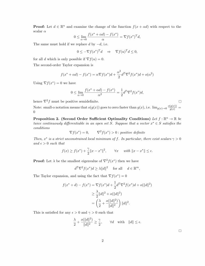
• Convex function with strict minimum

f(x) =1

2xT[

1 −1−1 4

]x

The critical point is the origin x = (0, 0), while the Hessian is

∇2f =

[1 −1−1 4

]and has eigenvalues λ1 ≈ 0.70 and λ2 ≈ 4.30 corresponding to eigenvectors v1 ≈ (−0.96,−0.29)and v2 ≈ (−0.29, 0.96).

−5

0

5

−5

0

5

0

20

40

60

80

100

120

140

160

180

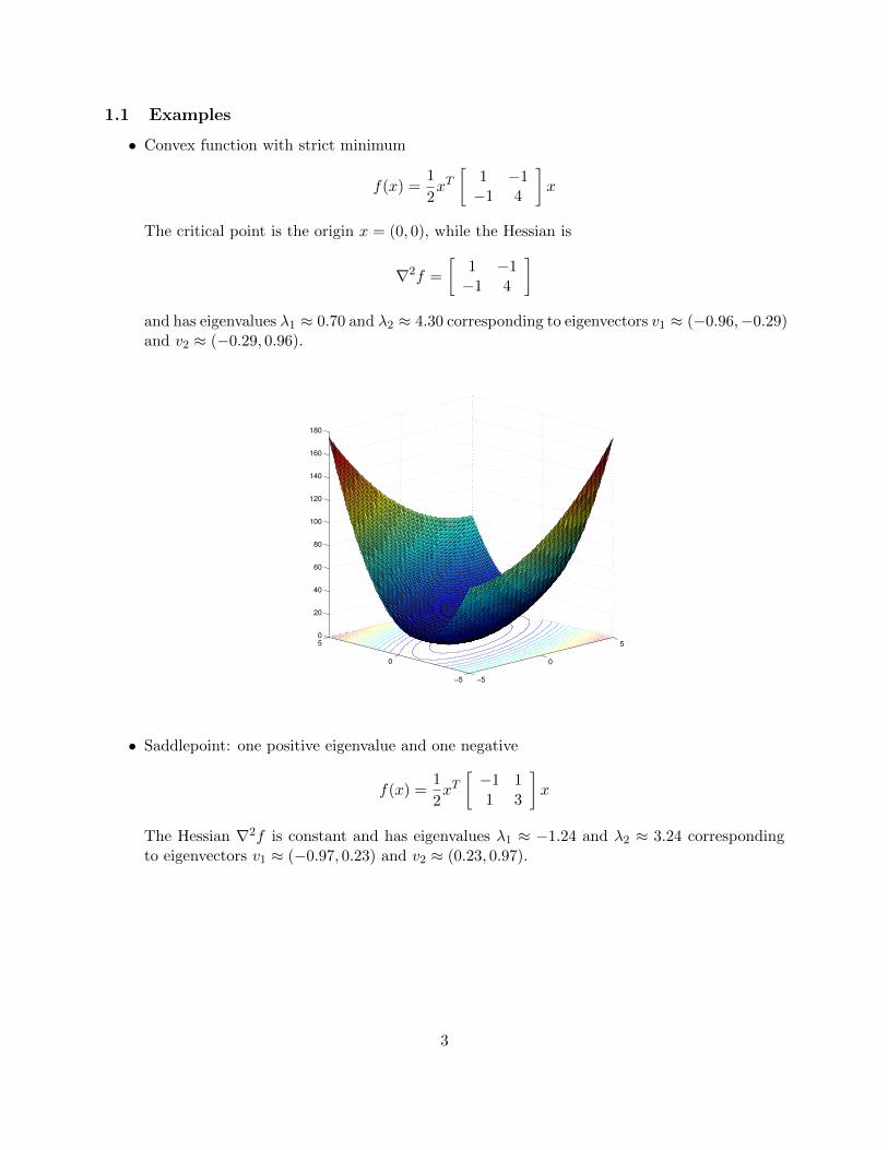
• Saddlepoint: one positive eigenvalue and one negative

f(x) =1

2xT[−1 11 3

]x

The Hessian ∇2f is constant and has eigenvalues λ1 ≈ −1.24 and λ2 ≈ 3.24 correspondingto eigenvectors v1 ≈ (−0.97, 0.23) and v2 ≈ (0.23, 0.97).

3

−5

0

5

−5

0

5

−40

−20

0

20

40

60

80

100

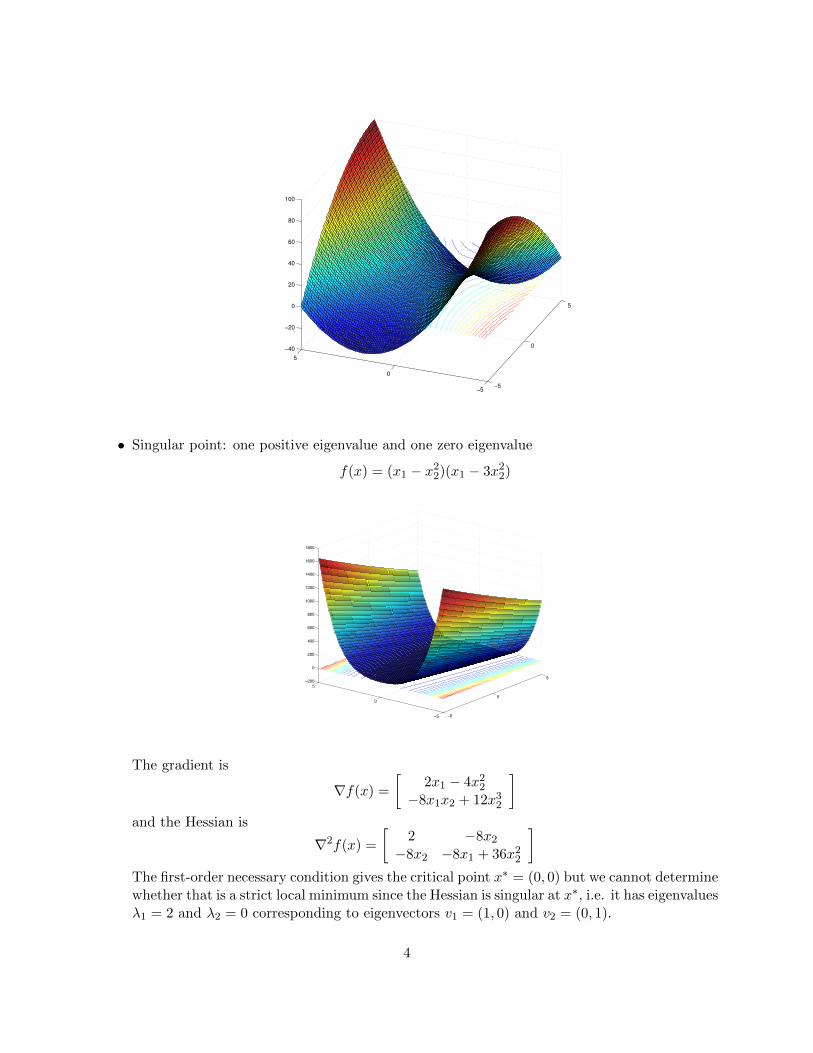
• Singular point: one positive eigenvalue and one zero eigenvalue

f(x) = (x1 − x22)(x1 − 3x22)

−5

0

5

−5

0

5

−200

0

200

400

600

800

1000

1200

1400

1600

1800

The gradient is

∇f(x) =

[2x1 − 4x22

−8x1x2 + 12x32

]and the Hessian is

∇2f(x) =

[2 −8x2−8x2 −8x1 + 36x22

]The first-order necessary condition gives the critical point x∗ = (0, 0) but we cannot determinewhether that is a strict local minimum since the Hessian is singular at x∗, i.e. it has eigenvaluesλ1 = 2 and λ2 = 0 corresponding to eigenvectors v1 = (1, 0) and v2 = (0, 1).

4

• a complicated function with multiple local minima

2 Numerical Solution: gradient-based methods

In general, optimality conditions for general nonlinear functions cannot be solved in closed-form.It is necessary to use an iterative procedure starting with some initial guess x = x0, i.e.

xk+1 = xk + αkdk, k = 0, 1, . . .

until f(xk) converges. Here dk ∈ Rn is called the descent direction (or more generally “searchdirection”) and αk > 0 is called the stepsize. The most common methods for finding αk and dk aregradient-based. Some use only first-order information (the gradient only) while other additionallyuse higher-order (gradient and Hessian) information.

• Gradient-based methods follow the general guidelines:

1. Choose direction dk so that whenever ∇f(xk) 6= 0 we have

∇f(xk)Tdk < 0,

i.e. the direction and negative gradient make an angle < 90◦

2. Choose stepsize αk > 0 so that

f(xk + αdk) < f(xk),

i.e. cost decreases

• Cost reduction is guaranteed (assuming ∇f(xk) 6= 0) since we have

f(xk+1) = f(xk) + αk∇f(xk)Tdk + o(αk)

and there always exist αk small enough so that

αk∇f(xk)Tdk + o(αk) < 0.

5

2.1 Selecting Descent Direction d

Descent direction choices

• Many gradient methods are specified in the form

xk+1 = xk − αkDk∇f(xk),

where Dk is positive definite symmetric matrix.

• Since dk = −Dk∇f(xk) and Dk > 0 the descent condition

−∇f(xk)TDk∇f(xk) < 0,

is satisfied.

We have the following general methods:

Steepest Descent

Dk = I, k = 0, 1, . . . ,

where I is the identity matrix. We have

∇f(xk)Tdk = −‖∇f(xk)‖2 < 0, when ∇f(xk) 6= 0

Furthermore, the direction ∇f(xk) results in the fastest decrease of f at α = 0 (i.e. near xk).

Newton’s Method

Dk = [∂2f(xk)]−1, k = 0, 1, . . . ,

provided that ∂2f(xk) > 0.

• The idea behind Newton’s method is to minimize a quadratic approximation of f around xk

fk(x) = f(xk) +∇f(xk)T (x− xk) +1

2(x− xk)T∇2f(xk)(x− xk),

and solve the condition ∇fk(x) = 0

• This is equivalent to∇f(xk) +∇2f(xk)(x− xk) = 0

and results in the Newton iteration

xk+1 = xk − [∇2f(xk)]−1∇f(xk)

6

Diagonally Scaled Steepest Descent

Dk =

dk1 0 0 · · · 0 0 00 dk2 0 · · · 0 0 0...

......

. . ....

...0 0 0 · · · 0 dkn−1 00 0 0 · · · 0 0 dkn

≡ diag([dk1, · · · , dkn]),

for some dki > 0. Usually these are the inverted diagonal elements of the hessian ∇2f , i.e.

dki =

[∂2f(xk)

(∂xi)2

]−1, k = 0, 1, . . . ,

Gauss-Newton Method

When the cost has a special least squares form

f(x) =1

2‖g(x)‖2 =

1

2

m∑i=1

(gi(x))2

we can choose

Dk =[∇g(xk)∇g(xk)T

]−1, k = 0, 1, . . .

Conjugate-Gradient Methods

Idea is to choose linearly independent (i.e. conjugate) search directions dk at each iteration. Forquadratic problems convergence is guaranteed by at most n iterations. Since there are at most nindependent directions, the independence condition is typically reset every k ≤ n steps for generalnonlinear problems.

The directions are computed according to

dk = −∇f(xk) + βkdk−1.

The most common way to compute βk is

βk =∇f(xk)T

(∇f(xk)−∇f(xk−1)

)∇f(xk−1)T∇f(xk−1)

It is possible to show that the choice βk ensures the conjugacy condition.

2.2 Selecting Stepsize α

• Minimization Rule: choose αk ∈ [0, s] so that f is minimized, i.e.

f(xk + αkdk) = minα∈[0,s]

f(xk + αdk)

which typically involves a one-dimensional optimization (i.e. a line-search) over [0, s].

7

• Successive Stepsize Reduction - Armijo Rule: idea is to start with initial stepsize s and ifxk + sdk does not improve cost then s is reduced:

Choose: s > 0, 0 < β < 1, 0 < σ < 1

Increase: m = 0, 1, ...

Until: f(xk)− f(xk + βmsdk) ≥ −σβms∇f(xk)Tdk

where β is the rate of decrease (e.g. β = .25) and σ is the acceptance ratio (e.g. σ = .01).

• Constant Stepsize: use a fixed step-size s > 0

αk = s, k = 0, 1, . . .

while simple it can be problematic: too large step-size can result in divergence; too small inslow convergence

• Diminishing Stepsize: use a stepsize converging to 0

αk → 0

under a condition∑∞

k=0 αk =∞, xk will converge theoretically but in practice is slow.

2.3 Example

• Consider the function f : R2 → R

f(x) = x1 exp(−(x21 + x22)) + (x21 + x22)/20

The gradient and Hessian are

∇f(x) =

[x1/10 + exp(−x21 − x22)(1− 2x21)x2/10− 2x1x2 exp(−x21 − x22)

],

∇2f(x) =

[(4x31 − 6x1) exp(−x21 − x22) + 1/10 (4x21x2 − 2x2) exp(−x12 − x22)

(4x21x2 − 2x2) exp(−x21 − x22) (4x1x22 − 2x1) exp(−x21 − x22) + 1/10

].

−2

−1

0

1

2

−2

−1

0

1

2−0.5

0

0.5

x1

x1 exp(−x

1

2−x

2

2)+...+x

2

2 (1.0/2.0e1)

x2

8

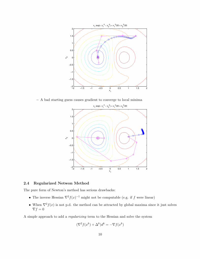
• The function has a strict global minimum around x∗ = (−2/3, 0) but also local minima

• There are also saddle points around x = (1, 1.5)

• We compare gradient-method (blue) and Newton method (magenta)

– Gradient converges (but takes many steps); ∇2f is not p.d. and Newton get stuck

x1

x2

x1 exp(− x

1

2 − x

2

2) + x

1

2/20 + x

2

2/20

−2 −1.5 −1 −0.5 0 0.5 1 1.5 2−2

−1.5

−1

−0.5

0

0.5

1

1.5

2

– Both methods converge if started near optimum; gradient zigzags

x1

x2

x1 exp(− x

1

2 − x

2

2) + x

1

2/20 + x

2

2/20

−1 −0.9 −0.8 −0.7 −0.6 −0.5 −0.4 −0.3 −0.2 −0.1 0

−0.5

0

0.5

1

– Newton’s methods with regularization (trust-region) now works

9

x1

x2

x1 exp(− x

1

2 − x

2

2) + x

1

2/20 + x

2

2/20

−2 −1.5 −1 −0.5 0 0.5 1 1.5 2−2

−1.5

−1

−0.5

0

0.5

1

1.5

2

– A bad starting guess causes gradient to converge to local minima

x1

x2

x1 exp(− x

1

2 − x

2

2) + x

1

2/20 + x

2

2/20

−2 −1.5 −1 −0.5 0 0.5 1 1.5 2−2

−1.5

−1

−0.5

0

0.5

1

1.5

2

2.4 Regularized Netwon Method

The pure form of Newton’s method has serious drawbacks:

• The inverse Hessian ∇2f(x)−1 might not be computable (e.g. if f were linear)

• When ∇2f(x) is not p.d. the method can be attracted by global maxima since it just solves∇f = 0

A simple approach to add a regularizing term to the Hessian and solve the system

(∇2f(xk) + ∆k)dk = −∇f(xk)

10

where the matrix ∆k is chosen so that

∇2f(xk) + ∆k > 0.

There are several ways to choose ∆k. In trust-region methods one sets

∆k = δkI,

where δk > 0 and I is the identity matrix.Newton’s method is derived by finding the direction d which minimizes the local quadratic

approximation fk of f at xk) defined by

fk(d) = f(xk) +∇f(xk)Td+1

2dT∇2f(xk)d.

It can be shown that the resulting method

(∇2f(xk) + δkI)dk = −∇f(xk)

is equivalent to solving the the optimization problem

dk ∈ arg min‖d‖≤γk

fk(d).

The restricted direction d must satisfy ‖d‖ ≤ γk, which is referred to as the trust region.

References

[1] D. P. Bertsekas. Nonlinear Programming, 2nd ed. Athena Scientific, Belmont, MA, 2003.

11