Embed Size (px)
Citation preview
Partnership for AiR Transportation Noise and Emissions ReductionAn FAA/NASA/Transport Canada-sponsored Center of Excellence
En Route Traffic Optimization to Reduce Environmental Impact
PARTNER Project 5 report
prepared by
John-Paul Clarke, Marcus Lowther, Liling Ren, William Singhose, Senay Solak, Adan Vela, Lawrence Wong
July 2008
REPORT NO. PARTNER-COE-2008-005
En Route Traffic Optimization
to Reduce Environmental Impact
Dr. John-Paul Clarke
Marcus Lowther Dr. Liling Ren
Dr. William Singhose Dr. Senay Solak
Adan Vela Lawrence Wong
PARTNER Report No.: PARTNER-COE-2008-001
July 2008
This work was funded by the U.S. Federal Aviation Administration Office of Environment and Energy, under Grant 03-C-NE-MIT, Amendment Nos. 028 and 30. The En Route Traffic Optimization to Reduce Environmental Impact Project is managed by Dr. John-Paul Clarke. Opinions, findings, and conclusions or recommendations expressed in this material are those of the authors and do not necessarily reflect the views of the FAA, NASA, or Transport Canada. The Partnership for AiR Transportation Noise and Emissions Reduction — PARTNER — is a cooperative aviation research organization, and an FAA/NASA/Transport Canada-sponsored Center of Excellence. PARTNER fosters breakthrough technological, operational, policy, and workforce advances for the betterment of mobility, economy, national security, and the environment. The organization's operational headquarters is at the Massachusetts Institute of Technology.
The Partnership for AiR Transportation Noise and Emissions Reduction Massachusetts Institute of Technology, 77 Massachusetts Avenue, 37-395
Cambridge, MA 02139 USA http://www.partner.aero
En Route Traffic Optimization
to Reduce Environmental Impact
Dr. John-Paul Clarke
Marcus Lowther Dr. Liling Ren
Dr. William Singhose Dr. Senay Solak
Adan Vela Lawrence Wong
PARTNER-COE-2008-005
This work was funded by the U.S. Federal Aviation Administration Office of Environment and Energy, under Grant 03-C-NE-MIT, Amendment Nos. 028 and 30. The En Route Traffic
Optimization to Reduce Environmental Impact Project is managed by Dr. John-Paul Clarke.
Any opinions, findings, and conclusions or recommendations expressed in this material are those of the author(s) and do not necessarily reflect the views of the FAA, NASA or Transport Canada
1
TABLE OF CONTENTS
1. PROJECT OVERVIEW..........................................................................................................................4 2. EN ROUTE TRAFFIC OPTIMIZATION .................................................................................................5
2.1. PRIOR RESEARCH IN CONFLICT RESOLUTION......................................................................................5 2.2. METHODOLOGY OVERVIEW................................................................................................................5 2.3. PROBLEM DESCRIPTION.....................................................................................................................6 2.4. SEPARATION CONSTRAINTS ...............................................................................................................8 2.5. COST FORMULATION .......................................................................................................................10
2.5.1. Fuel Costs due to Change in Airspeed ..................................................................................10 2.5.2. Fuel Costs due to Change in Heading Angle.........................................................................13 2.5.3. Total Cost Function................................................................................................................16
2.6. COMPUTATIONAL STUDY FOR STATIC CONFLICT RESOLUTION ...........................................................16 2.7. DYNAMIC CONFLICT RESOLUTION ALGORITHM..................................................................................18 2.8. COMPUTATIONAL STUDY FOR DYNAMIC CONFLICT RESOLUTION USING CLEVELAND ARTCC DATA .....19
2.8.1. Case Study Results ...............................................................................................................21 2.8.2. Generating Fuel Curves with Wind Field Effect .....................................................................24
2.9. EN ROUTE TRAFFIC OPTIMIZATION CONCLUSIONS ...........................................................................25 3. EN ROUTE SPEED CHANGE OPTIMIZATION FOR CONTINUOUS DESCENT ARRIVALS..........27
3.1. STATE OF THE ART LIMITATIONS.......................................................................................................28 3.2. EN ROUTE SPEED ALTERATION FORMULATIONS ...............................................................................29
3.2.1. One Speed-Change Formulation...........................................................................................29 3.2.2. One Speed Change Algorithm While Minimizing Initial and Final ETA Difference................31 3.2.3. Fairness Considerations in Speed Alteration Algorithms ......................................................33 3.2.4. Variable Sequence Constraints .............................................................................................34
3.3. COMPUTATIONAL STUDY FOR THE EN ROUTE SPACING PROGRAM.....................................................35 3.3.1. Sample CDA Flight Test Case...............................................................................................35 3.3.2. Test Case Results..................................................................................................................36
3.4. CONCLUSIONS AND FUTURE WORK FOR EN ROUTE SPEED CHANGE OPTIMIZATION............................45 4. FUTURE WORK ..................................................................................................................................47 ACKNOWLEDGEMENTS...........................................................................................................................48 APPENDIX A-DERIVATION OF MACH-TIME RELATIONSHIP...............................................................49 APPENDIX B- NOMENCLATURE FOR EN ROUTE TRAFFIC OPTIMIZATION .....................................52 APPENDIX C- NOMENCLATURE FOR EN ROUTE SPREED CHANGE OPTIMIZATION FOR CONTINUOUS DESCENT ARRIVALS ......................................................................................................53 REFERENCES............................................................................................................................................54
2
Principal Investigator
John-Paul Clarke, Ph.D. Associate Professor
School of Aerospace Engineering Georgia Institute of Technology
Members of the Project Team
Marcus Lowther Graduate Research Assistant
School of Aerospace Engineering Georgia Institute of Technology
Liling Ren, Sc.D. Research Engineer
School of Aerospace Engineering Georgia Institute of Technology
William Singhose, Ph.D. Associate Professor
School of Mechanical Engineering Georgia Institute of Technology
Senay Solak, Ph.D. Independent Consultant
Adan Vela Graduate Research Assistant
School of Mechanical Engineering Georgia Institute of Technology
Lawrence Wong Undergraduate Research Assistant School of Aerospace Engineering Georgia Institute of Technology
3
1. Project Overview
Air traffic delays due to congestion in the National Airspace System (NAS) are a source of unnecessary cost to airlines, passengers, and air transportation dependent businesses. Congestion is estimated to cost the aviation industry, passengers, and shippers approximately $10 billion per year [Deehan, 2006]. This cost can be further segregated into a $6 billion impact upon direct airline operating costs and a $4 billion impact upon the value of collective passenger time.
Delays also have an environmental cost. Because of congestion, aircraft are often forced to fly far from the cruise altitude and/or the cruise speed for which they are designed. Such sub-optimality results in unnecessary fuel burn and gaseous emission that give rise to environmental concerns both globally and locally at ground level. The significant magnitude of air traffic delays presently observed is an indication that the current air traffic control infrastructure is not capable of handing current traffic levels. Given the forecast growth in aviation over the next decade there is an urgent need air traffic control decision-support or automation tools to address the problem of congestion in the NAS.
In this report, we propose methods to investigate and quantify the economic and environmental benefits of optimization tools that en route air traffic controllers could use. More specifically, we develop mathematical models for conflict-free optimal trajectories over a volume of airspace and for continuous descent arrivals. We present computational studies and demonstrate savings due to proposed algorithms using traffic through Cleveland Air Route Traffic Control Center (ARTCC), one of the most congested airspaces in the US.
We also determine the environmental benefits in terms of the change in the amount of emissions that are produced by aircraft. The fuel burn is determined using data for aircraft performance and fuel burn that has been made available through an on-going nondisclosure agreement with Boeing, and using Base of Aircraft Data (BADA) in the case of other aircraft where this data is not available.
Overall, prototype algorithms for a tool that air traffic controllers could use to optimally control aircraft are developed. This also enables the quantification of the economic and environmental benefits of optimization in en route airspace. The two main sections of this report are structured as follows: In Section 2, we study en route traffic optimization and develop static and dynamic conflict resolution algorithms to optimally route aircraft. In Section 3, we consider arriving aircraft only, and describe a speed-change based optimization procedure for use in a continuous descent arrival context.
4
5
2. En Route Traffic Optimization
Development of advanced air traffic conflict detection and resolution algorithms is important to the overall improvement of the air traffic management (ATM) system. This is especially true when one considers issues of safety and capacity within the context of growing air traffic, as well as their environmental implications.
In this section, we consider optimizing tactical control of aircraft to maintain separation while considering associated fuel costs with any heading deviation or speed changes. Safety requirements are considered as hard constraints that must be maintained. The objective function of the optimization program focuses on minimizing fuel costs, and hence the resulting environmental impact.
A conflict in air traffic occurs when two or more aircraft encroach the minimum required separation, as defined by the regulator. Conflict detection is the identification of potential conflicts through prediction of future aircraft trajectories based on their current positions, headings and flight plans. Once a conflict is detected, it is resolved by changing the flight plan of one or more aircraft so that the minimum separation requirements are satisfied. However, the overall goal is to ensure conflict-free optimal trajectories for all aircraft from entrance to exit within a volume of airspace. In this regard, we first develop a static conflict resolution algorithm, and then use it to dynamically create conflict-free trajectories for aircraft.
2.1. Prior Research in Conflict Resolution
Aircraft conflict detection and resolution has been studied extensively in the literature. A comprehensive survey of the proposed models is presented in Kuchar and Yang (2000). Since the publication of that survey, several other methods have been introduced. The approaches developed over the past few years include a 3D model based on a collision cone approach (Goss et al. 2004). However, the solution of the model requires significant computational effort. Another computationally intensive approach, suggested by the authors of Hu et al. (2002), requires the identification of all conflict-free maneuvers, and the selection of the best such maneuver. In another recent study, the authors of Vivona et al. (2006) suggest a genetic algorithm approach based on a predefined set of maneuvers for aircraft, while the authors of Idris et al. (2003) describe a time-based conflict resolution algorithm.
There exist two recent conflict resolution models that are directly related to the approach described in this study. Both of these methods contain integer programming models, which enable relatively fast calculations of an optimal conflict resolution procedure. In the first study, Pallottino et al. (2002), an integer programming model is developed by assuming that aircraft can perform either a speed change or a heading change, but not both. The objective of the conflict resolution algorithm is defined as the minimization of the maximum deviation in the changes made. In the second study, Hylkema and Visser (2003), a similar integer programming model, that also accounts for controller workload is discussed. However, the model again assumes that only heading changes are allowed to resolve conflict.
2.2. Methodology Overview
In this report, we significantly extend ideas presented in Pallottino et al. (2002) to a more general case where both heading and speed changes are allowed, and where more complex objectives are considered, including minimization of fuel costs required to return to the desired flight path after a heading change.
In Kuchar and Yang (2000), the existing conflict detection and resolution methods are characterized according to considered scope, dimensions, resolution methodology and maneuvers. Following this categorization, our proposed approach is a global conflict resolution procedure for all aircraft that are involved in a conflict. Although, the conflict resolution procedure is described in the horizontal plane only, adaptation to vertical planes is done simply by assuming multiple horizontal layers and introducing variables modeling the movements between these layers.
The developed mathematical model, resulting in a mixed integer linear program, provides a broad framework for resolving conflicts through fast numerical optimization methods, and allows for both heading and speed changes. Particular focus has been placed on reducing fuel costs involved in conflict resolution. As noted earlier, this is important given the significant role that fuel plays in the operating cost of aircraft and the growing concern regarding the impact of gaseous emissions on the environment. Another significant aspect of the proposed approach is the ability to solve a complex problem in near real-time for conflicts involving a large number of aircraft. Hence, in addition to real time implementations, the proposed model can be used within test and simulation environments for air traffic control such as in capacity calculations of sectors or in studies of the free flight concept.
The following subsections provide a general description of the problem; the mathematical descriptions of the separation constraints required for conflict resolution; linear approximations of the complex fuel cost structures; results of the computational studies performed; method for real-time implementation in a center environment, and subsequent analysis.
2.3. Problem Description
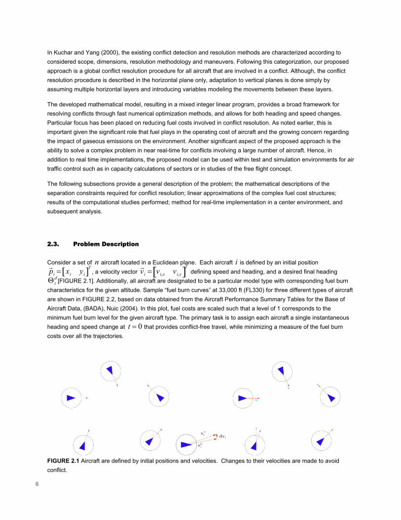
Consider a set of aircraft located in a Euclidean plane. Each aircraft i is defined by an initial position , a velocity vector
defining speed and heading, and a desired final heading
[
n]
r p i = xi yi[ T
Θ id
r v i = vi,x vi,y[ T
0
]FIGURE 2.1]. Additionally, all aircraft are designated to be a particular model type with corresponding fuel burn
characteristics for the given altitude. Sample “fuel burn curves” at 33,000 ft (FL330) for three different types of aircraft are shown in FIGURE 2.2, based on data obtained from the Aircraft Performance Summary Tables for the Base of Aircraft Data, (BADA), Nuic (2004). In this plot, fuel costs are scaled such that a level of 1 corresponds to the minimum fuel burn level for the given aircraft type. The primary task is to assign each aircraft a single instantaneous heading and speed change at that provides conflict-free travel, while minimizing a measure of the fuel burn costs over all the trajectories.
t =
FIGURE 2.1 Aircraft are defined by initial positions and velocities. Changes to their velocities are made to avoid conflict.
6
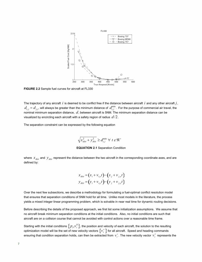
FIGURE 2.2 Sample fuel curves for aircraft at FL330
The trajectory of any aircraft is deemed to be conflict free if the distance between aircraft and any other aircrafti i j ,
, will always be greater than the minimum distance of . For the purpose of commercial air travel, the nominal minimum separation distance, , between aircraft is 5NM. The minimum separation distance can be visualized by encircling each aircraft with a safety region of radius .
di, j = d j,i di, jmin
d /2d
The separation constraint can be expressed by the following equation
xdist2 + ydist
2 ≥ di, jmin ∀ t ε ℜ+
EQUATION 2.1 Separation Condition
where xdist and represent the distance between the two aircraft in the corresponding coordinate axes, and are defined by:
ydist
xdist = xi + vi,xt( )− x j + v j,xt( )
ydist = yi + vi,yt( )− y j + v j,yt( ) Over the next few subsections, we describe a methodology for formulating a fuel-optimal conflict resolution model that ensures that separation conditions of 5NM hold for all time. Unlike most models in the literature, the process yields a mixed integer linear programming problem, which is solvable in near real time for dynamic routing decisions.
Before describing the details of the proposed approach, we first list some initialization assumptions. We assume that no aircraft break minimum separation conditions at the initial conditions. Also, no initial conditions are such that aircraft are on a collision course that cannot be avoided with control actions over a reasonable time frame.
Starting with the initial conditions , the position and velocity of each aircraft, the solution to the resulting optimization model will be the set of new velocity vectors
pi,vi0{ }
vi+{ } for all aircraft. Speed and heading commands
ensuring that condition separation holds, can then be extracted from vi+ . The new velocity vector represents the vi
+
7
solution for an instantaneous change in the trajectory. The model does not take into account the time to execute heading and speed changes. It is assumed that deviations are small and the time to complete any maneuver fix is small in comparison to time to the conflict. However, the safety region about each aircraft can be expanded to handle uncertainty from resulting maneuver changes, wind variation, or other unmodeled phenomena.
2.4. Separation Constraints
For conflict-free trajectories, each pair of aircraft must satisfy the separation constraints (EQUATION 2.1). In this section, the separation condition is deconstructed into a set of linear constraints that ensure no aircraft encroaches another aircraft's safety region. This approach is similar to the one used in Pallottino et al. (2002) to determine the separation constraints.
Consider a pair of aircraft and i j with initial position and velocity states:
pi = xi,yi( ), vi
0 = vi,x0 ,vi,y
0( )
p j = x j ,y j( ), v j0 = v j,x
0 ,v j,y0( )
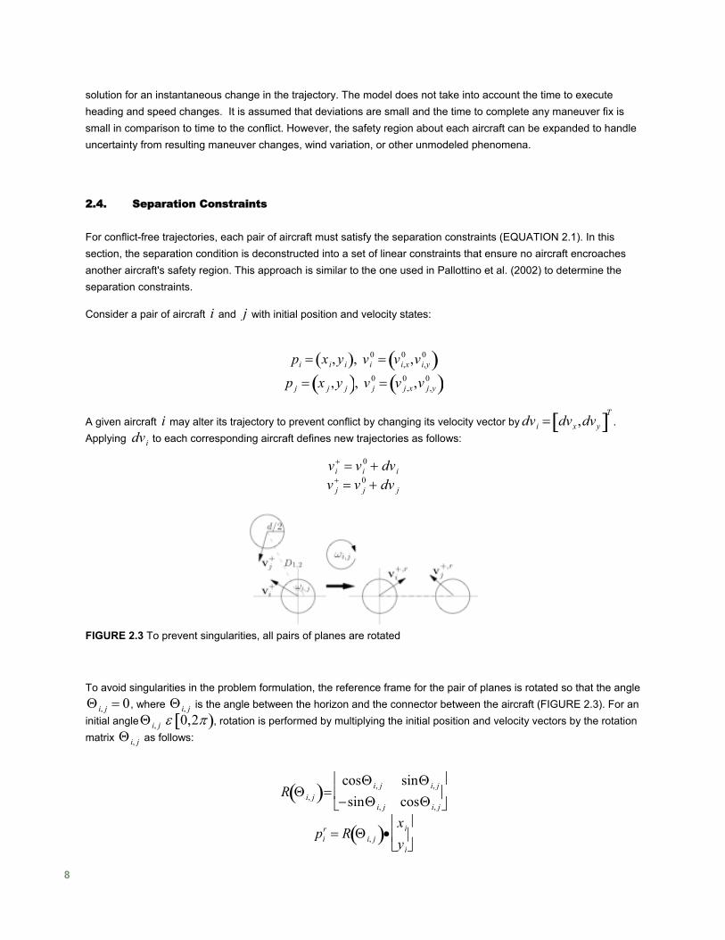
A given aircraft may alter its trajectory to prevent conflict by changing its velocity vector by . Applying to each corresponding aircraft defines new trajectories as follows:
i dvi = dvx ,dvy[ ]T
dvi
vi+ = vi
0 + dvi v j
+ = v j0 + dv j
FIGURE 2.3 To prevent singularities, all pairs of planes are rotated
To avoid singularities in the problem formulation, the reference frame for the pair of planes is rotated so that the angle
, where Θ is the angle between the horizon and the connector between the aircraft (Θ i, j = 0 i, j FIGURE 2.3). For an initial angle Θ i, j ε 0,2π[ ), rotation is performed by multiplying the initial position and velocity vectors by the rotation matrix as follows: Θ i, j
R Θ i, j( )=cosΘ i, j sinΘ i, j
−sinΘ i, j cosΘ i, j
⎡
⎣ ⎢
⎤
⎦ ⎥
pir = R Θ i, j( )•
xi
yi
⎡
⎣ ⎢
⎤
⎦ ⎥
8
vi+,r = R Θ i, j( )• vi
+
p jr = R Θ i, j( )•
x j
y j
⎡
⎣ ⎢
⎤
⎦ ⎥
v j+,r = R Θ i, j( )• v j
+ Once the rotation is performed, a set of linear constraints to ensure that a pair of aircraft maintains separation is derived from the relative velocity of aircraft i to aircraft˜ v i, j j , i.e.
˜ v i, j = vi
+,r − v j+,r
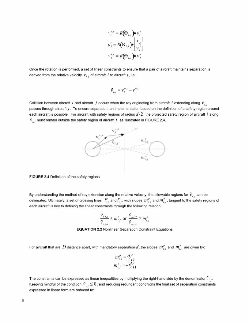
Collision between aircraft i and aircraft j occurs when the ray originating from aircraft i extending along passes through aircraft
˜ v i, jj . To ensure separation, an implementation based on the definition of a safety region around
each aircraft is possible. For aircraft with safety regions of radius , the projected safety region of aircraft along must remain outside the safety region of aircraft
d /2 i˜ v i, j j , as illustrated in FIGURE 2.4.
FIGURE 2.4 Definition of the safety regions
By understanding the method of ray extension along the relative velocity, the allowable regions for can be delineated. Ultimately, a set of crossing lines, and , with slopes and , tangent to the safety regions of each aircraft is key to defining the linear constraints through the following relation:
˜ v i, jli, j
p li, jn mi, j
p mi, jn
˜ v i, j ,y
˜ v i, j ,x
≤ mi, jn or
˜ v i, j ,y
˜ v i, j ,x
≥ mi, jp
EQUATION 2.2 Nonlinear Separation Constraint Equations
For aircraft that are distance apart, with mandatory separation , the slopes and are given by: D d mi, j
p mi, jn
mi, jp = d
D
mi, jn = −d
D
The constraints can be expressed as linear inequalities by multiplying the right-hand side by the denominator . Keeping mindful of the condition , and reducing redundant conditions the final set of separation constraints expressed in linear form are reduced to:
˜ v i, j˜ v i, j ≤ 0
9

˜ v i, j,y ≤ ˜ v i, j,xmi, j
n
˜ v i, j,x ≥ 0 or or
˜ v i, j,y ≥ ˜ v i, j,xmi, jp
˜ v i, j,x ≥ 0˜ v i, j,x ≤ 0
EQUATION 2.3 Linear separation constraints
The above constraints (EQUATION 2.3) are expressed as linear inequalities of the decisions variables and
, which are functions of the speed and heading changes, , to be made to ensure separation. Furthermore, the condition allows for the case of aircrafts trailing one another, i.e. the singularity of in the slope is admissible for this formulation. The constraints are then applied to all pairs of aircraft. As the constraints are reciprocal, only one set of constraints is required for each pair.
˜ v i, j ,x
= 0˜ v i, j ,y dvi,
˜ v i, j,x ≤ 0 ˜ v i, j,x
Note that if avoidance is required to route an aircraft around a no-fly region, moving weather formation, or any type of obstacle, then the same process can be used to form the set of linear constraints. For a non-moving obst cle, it is assumed that . The slopes for and are given by
advobs = 0 li, j
p li, jn mi, j
p =d + dobs
2D, and mi, j
p = −d + dobs
2D, where
can be selected as the diameter of the smallest circle encircling the obstacle. dobs
2.5. Cost Formulation
In line with the primary goal of providing a framework in which fuel costs are considered in conflict resolution and aircraft routing, an appropriate cost function G0 s,Θ( ) can be defined as:
G0 s,Θ( )= gs s( )+ gh Θ( )
where and are nonlinear scalar functions of the airspeeds , and the headings of the aircraft. The function measures the fuel burn percentage of an aircraft, while
gs s( )gs s(
gh Θ( ) sh
Θ) g Θ( ) accounts for the scaled increase in
distance traveled due to a deviation from the desired route. Considering both parts, G0 s,Θ( ) is the fuel consumption percentage with respect to the optimal path at a desired airspeed when there are no obstacles.
The measures and Θ, and thus the cost functions s gs s( ) and gh Θ( ), are nonlinear nonconvex functions of the decision variables . In the following sections, we develop tight convex linear approximations for these functions, and show that the underlying optimization problem can be modeled.
dvi
2.5.1. Fuel Costs due to Change in Airspeed
Previous conflict resolution research has focused on minimizing the velocity deviation, , that an aircraft is required to make to ensure separation. Noting that any such deviation incurs costs, a measure of airspeed is required to provide a broader framework to understand and study the fairness and costs associated with routing of the aircraft. The final airspeed of aircraft ,
dvi
i si+ , for determination of fuel burn can be calculated according to a first-
order approximation:
10
si+ ~ si
0 +1si
0 vi,x0 vi,y
0[ ]dvi = ˆ s i
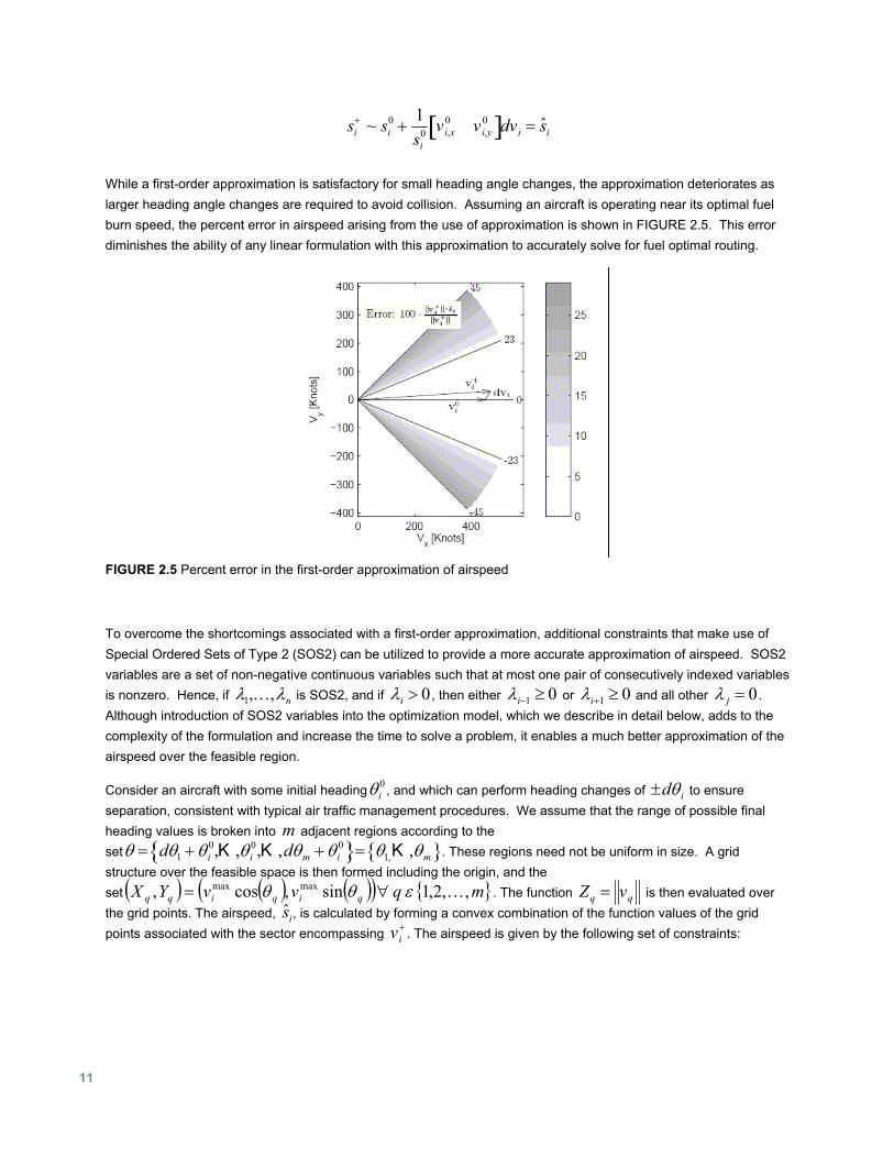
While a first-order approximation is satisfactory for small heading angle changes, the approximation deteriorates as larger heading angle changes are required to avoid collision. Assuming an aircraft is operating near its optimal fuel burn speed, the percent error in airspeed arising from the use of approximation is shown in FIGURE 2.5. This error diminishes the ability of any linear formulation with this approximation to accurately solve for fuel optimal routing.
FIGURE 2.5 Percent error in the first-order approximation of airspeed
To overcome the shortcomings associated with a first-order approximation, additional constraints that make use of Special Ordered Sets of Type 2 (SOS2) can be utilized to provide a more accurate approximation of airspeed. SOS2 variables are a set of non-negative continuous variables such that at most one pair of consecutively indexed variables is nonzero. Hence, if λ1,K,λn is SOS2, and if λi > 0 , then either λi−1 ≥ 0 or λi+1 ≥ 0 and all other λ j = 0 . Although introduction of SOS2 variables into the optimization model, which we describe in detail below, adds to the complexity of the formulation and increase the time to solve a problem, it enables a much better approximation of the airspeed over the feasible region.
Consider an aircraft with some initial headingθi0 , and which can perform heading changes of ±dθi to ensure
separation, consistent with typical air traffic management procedures. We assume that the range of possible final heading values is broken into adjacent regions according to the set
m,dθθ = dθ1 + θi
0,K ,θi0,K m + θi
0{ }= K ,θmθ1,{ }. These regions need not be uniform in size. A grid structure over the feasible spa e is then form including the origin, and the set
c ed( ) ( ) ( )( ) { }m,KqvYX qqiqq ,2,1 sincos, maxmax εθθ= vi, ∀ . The function Zq = vq is then evaluated over
the grid points. The airspeed, , is calculated by forming a convex combination of the function values of the grid points associated with the sector encompassing v
ˆ s ii+ . The airspeed is given by the following set of constraints:
11
ˆ v i,x+ = Xqλq
q= 0
m
∑
ˆ v i,y+ = Yqλq
q= 0
m
∑
ˆ s i = Zqλqq= 0
m
∑
λqq= 0
m
∑ =1
λq ε SOS2 ∀ q
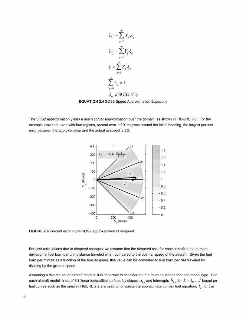
EQUATION 2.4 SOS2 Speed Approximation Equations
The SOS2 approximation yields a much tighter approximation over the domain, as shown in FIGURE 2.6. For the example provided, even with four regions, spread over ±45 degrees around the initial heading, the largest percent error between the approximation and the actual airspeed is 2%.
FIGURE 2.6 Percent error in the SOS2 approximation of airspeed
For cost calculations due to airspeed changes, we assume that the airspeed cost for each aircraft is the percent deviation in fuel burn per unit distance traveled when compared to the optimal speed of the aircraft. Given the fuel burn per minute as a function of the true airspeed, this value can be converted to fuel burn per NM traveled by dividing by the ground speed.
Assuming a diverse set of aircraft models, it is important to consider the fuel burn equations for each model type. For each aircraft model, a set of $l$ linear inequalities defined by slopes and intercepts b for ak,i k,i k =1,K, l based on fuel curves such as the ones in FIGURE 2.2 are used to formulate the approximate convex fuel equation, , for the ti
12
ith aircraft:
a1,iˆ s i + b1,i ≤ ti
a2,iˆ s i + b2,i ≤ ti
M
al,iˆ s i + bl,i ≤ ti
2.5.2. Fuel Costs due to Change in Heading Angle
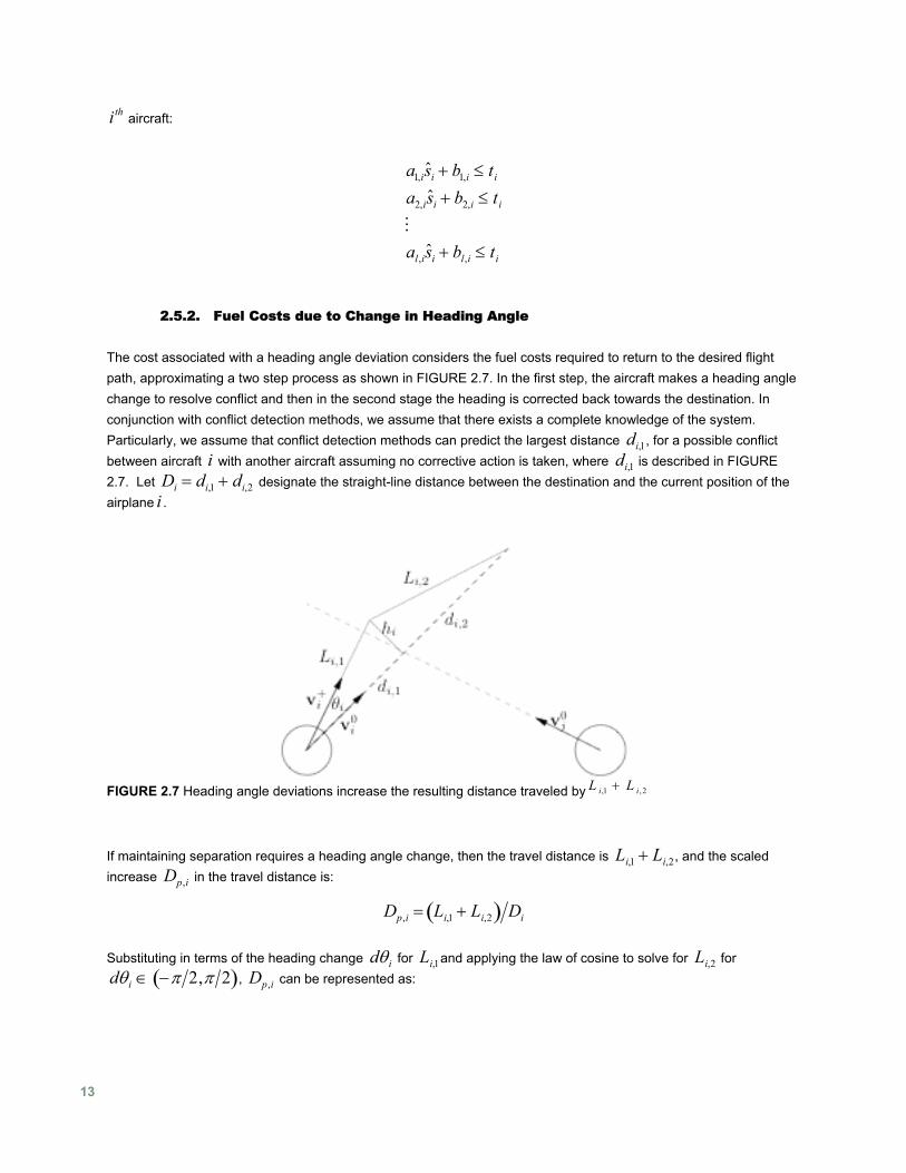
The cost associated with a heading angle deviation considers the fuel costs required to return to the desired flight path, approximating a two step process as shown in FIGURE 2.7. In the first step, the aircraft makes a heading angle change to resolve conflict and then in the second stage the heading is corrected back towards the destination. In conjunction with conflict detection methods, we assume that there exists a complete knowledge of the system. Particularly, we assume that conflict detection methods can predict the largest distance , for a possible conflict between aircraft with another aircraft assuming no corrective action is taken, where is described in
di,1di,1i
i,1
FIGURE 2.7. Let designate the straight-line distance between the destination and the current position of the airplane .
Di = d + di,2i
FIGURE 2.7 Heading angle deviations increase the resulting distance traveled by L i,1 + L i , 2
If maintaining separation requires a heading angle change, then the travel distance is , and the scaled increase in the travel distance is:
Li,1 + Li,2Dp,i
Dp,i = Li,1 + Li,2( ) Di Substituting in terms of the heading change dθi for and applying the law of cosine to solve for for Li,1 Li,2dθi ∈ −π 2,π 2( ) p,i, D can be represented as:
13
Dp,i =di,1 cos dθi( )+ di,1 cos dθi( )( )2
+ Di2 − 2di,1Di
Di
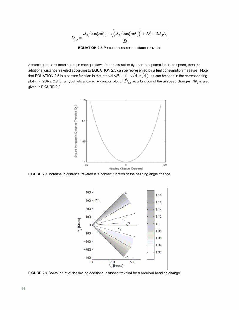
EQUATION 2.5 Percent increase in distance traveled
Assuming that any heading angle change allows for the aircraft to fly near the optimal fuel burn speed, then the additional distance traveled according to EQUATION 2.5 can be represented by a fuel consumption measure. Note that EQUATION 2.5 is a convex function in the interval dθi ∈ −π 4,π 4( ), as can be seen in the corresponding plot in FIGURE 2.8 for a hypothetical case. A contour plot of as a function of the airspeed changes is also given in
Dp,i dviFIGURE 2.9.
FIGURE 2.8 Increase in distance traveled is a convex function of the heading angle change
FIGURE 2.9 Contour plot of the scaled additional distance traveled for a required heading change
14
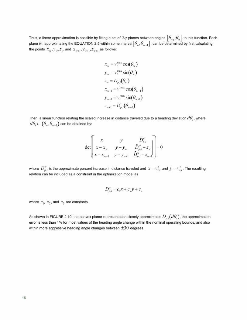
Thus, a linear approximation is possible by fitting a set of planes between angles 2q θ−q ,θq[ ] to this function. Each plane , approximating the w EQUATION 2.5 within some interval θw,θw+1[ ], can be determined by first calculating the points xw, yw,zw and xw+1, yw+1,zw+1 as follows:
xw = vi
max cos θw( )yw = vi
max sin θw( )zw = Dp,i θw( )xw+1 = vi
max cos θw+1( )yw+1 = vi
max sin θw+1( )zw+1 = Dp,i θw+1( )
Then, a linear function relating the scaled increase in distance traveled due to a heading deviation dθi , where dθi ∈ θw,θw+1( ) can be obtained by:
detx y ˆ D p,i
w
x − xw y − ywˆ D p,i
w − zw
x − xw+1 y − yw+1ˆ D p,i
w − zw+1
⎡
⎣
⎢ ⎢ ⎢
⎤
⎦
⎥ ⎥ ⎥
⎛
⎝
⎜ ⎜ ⎜
⎞
⎠
⎟ ⎟ ⎟
= 0
where is the approximate percent increase in distance traveled and Dp,i
w x = vi,x+ and . The resulting
relation can be included as a constraint in the optimization model as y = vi,y
+
Dp,i
w = c1x + c2y + c3 where , c , and are constants. c1 2 c3
As shown in FIGURE 2.10, the convex planar representation closely approximates Dp,i dθi( ), the approximation error is less than 1% for most values of the heading angle change within the nominal operating bounds, and also within more aggressive heading angle changes between ±30 degrees.
15
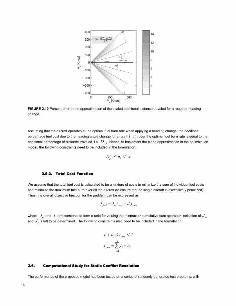
FIGURE 2.10 Percent error in the approximation of the scaled additional distance traveled for a required heading change.
Assuming that the aircraft operates at the optimal fuel burn rate when applying a heading change, the additional percentage fuel cost due to the heading angle change for aircraft i , , over the optimal fuel burn rate is equal to the additional percentage of distance traveled, i.e. . Hence, to implement the plane approximation in the optimization model, the following constraints need to be included in the formulation:
uiDp,i
ˆ D p,iw ≤ ui ∀ w
2.5.3. Total Cost Function
We assume that the total fuel cost is calculated to be a mixture of costs to minimize the sum of individual fuel costs and minimize the maximum fuel burn over all the aircraft (to ensure that no single aircraft is excessively penalized). Thus, the overall objective function for the problem can be expressed as:
f fuel = Jmtmax + Jstsum
where Jm and Js are constants to form a ratio for valuing the minmax or cumulative sum approach; selection of Jm and Js is left to be determined. The following constraints also need to be included in the formulation:
ti + ui ≤ tmax ∀ i
tsum = ti + uii=1
n
∑
2.6. Computational Study for Static Conflict Resolution
The performance of the proposed model has been tested on a series of randomly generated test problems, with
16
varying levels of complexity. The complexity of the generated models was measured according to the number of planes involved, and the density of the aircraft. Several different levels were considered for each of these two complexity measures, which resulted with the 30 configurations listed in Table 1. The number following the letter N in the test problem label represents the number of aircraft, while the number after the letter D is the length in nautical miles of a side of the square area considered for the problem. The instances were generated by positioning the aircraft randomly in the considered area according to a uniform distribution. In addition, the initial headings of the aircraft were selected such that the aircraft fly within a 90 degree angle towards the center of the area. Each of the test instances assumes a separation requirement of d = 5 NM.
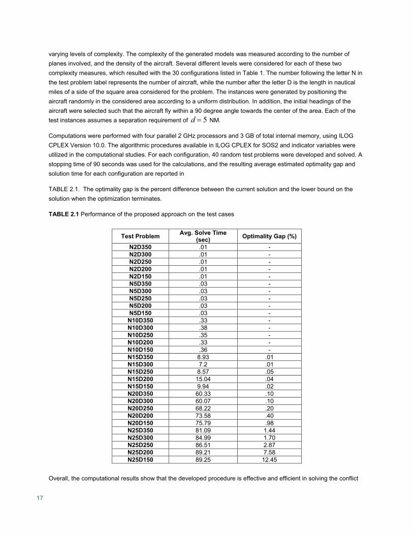
Computations were performed with four parallel 2 GHz processors and 3 GB of total internal memory, using ILOG CPLEX Version 10.0. The algorithmic procedures available in ILOG CPLEX for SOS2 and indicator variables were utilized in the computational studies. For each configuration, 40 random test problems were developed and solved. A stopping time of 90 seconds was used for the calculations, and the resulting average estimated optimality gap and solution time for each configuration are reported in
TABLE 2.1. The optimality gap is the percent difference between the current solution and the lower bound on the solution when the optimization terminates.
TABLE 2.1 Performance of the proposed approach on the test cases
Test Problem Avg. Solve Time (sec) Optimality Gap (%)
N2D350 .01 - N2D300 .01 - N2D250 .01 - N2D200 .01 - N2D150 .01 - N5D350 .03 - N5D300 .03 - N5D250 .03 - N5D200 .03 - N5D150 .03 -
N10D350 .33 - N10D300 .38 - N10D250 .35 - N10D200 .33 - N10D150 .36 - N15D350 8.93 .01 N15D300 7.2 .01 N15D250 8.57 .05 N15D200 15.04 .04 N15D150 9.94 .02 N20D350 60.33 .10 N20D300 60.07 .10 N20D250 68.22 .20 N20D200 73.58 .40 N20D150 75.79 .98 N25D350 81.09 1.44 N25D300 84.99 1.70 N25D250 86.51 2.87 N25D200 89.21 7.58 N25D150 89.25 12.45
Overall, the computational results show that the developed procedure is effective and efficient in solving the conflict
17
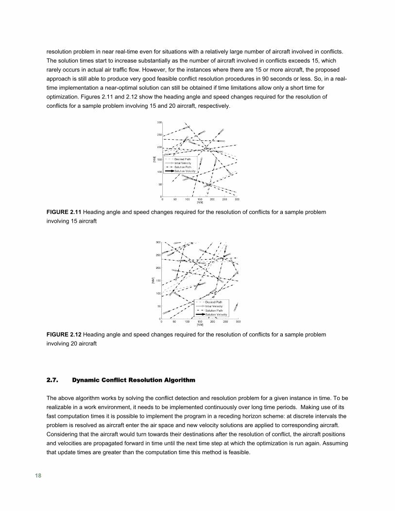
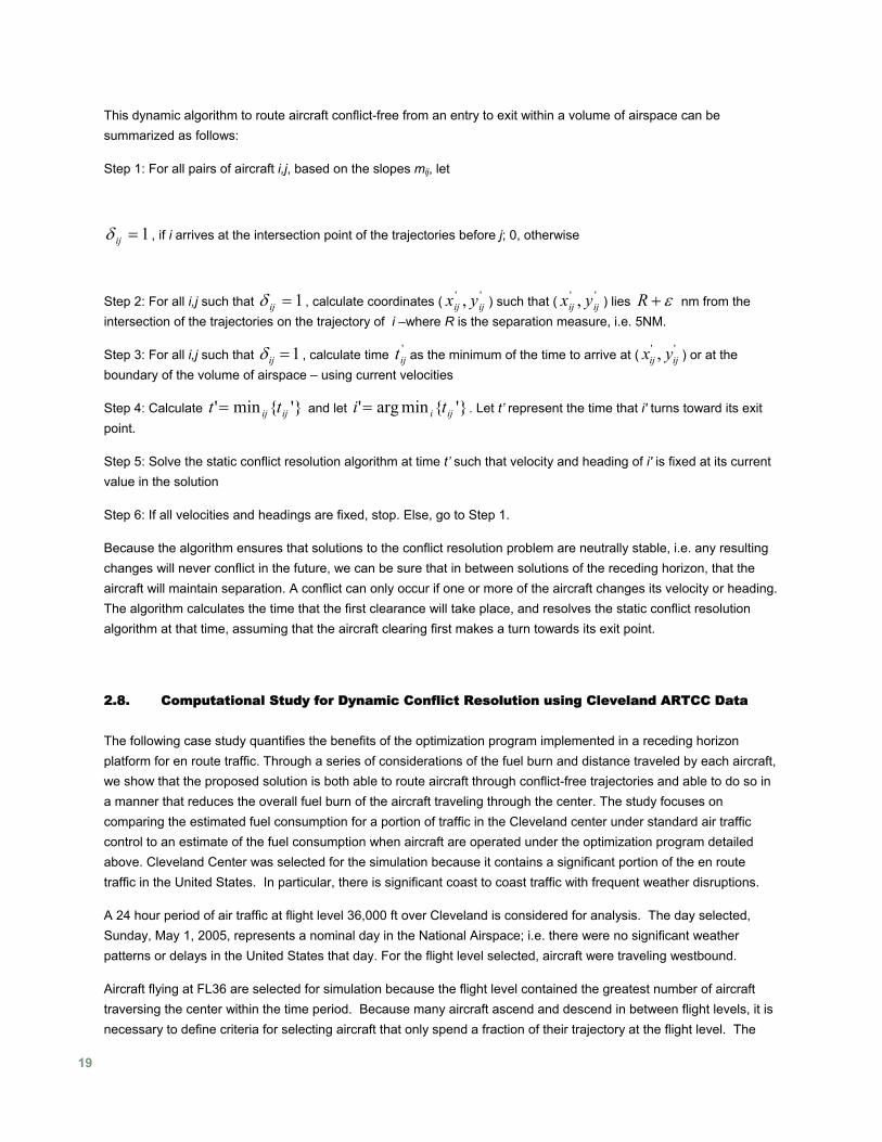
resolution problem in near real-time even for situations with a relatively large number of aircraft involved in conflicts. The solution times start to increase substantially as the number of aircraft involved in conflicts exceeds 15, which rarely occurs in actual air traffic flow. However, for the instances where there are 15 or more aircraft, the proposed approach is still able to produce very good feasible conflict resolution procedures in 90 seconds or less. So, in a real-time implementation a near-optimal solution can still be obtained if time limitations allow only a short time for optimization. Figures 2.11 and 2.12 show the heading angle and speed changes required for the resolution of conflicts for a sample problem involving 15 and 20 aircraft, respectively.
FIGURE 2.11 Heading angle and speed changes required for the resolution of conflicts for a sample problem involving 15 aircraft
FIGURE 2.12 Heading angle and speed changes required for the resolution of conflicts for a sample problem involving 20 aircraft
2.7. Dynamic Conflict Resolution Algorithm
The above algorithm works by solving the conflict detection and resolution problem for a given instance in time. To be realizable in a work environment, it needs to be implemented continuously over long time periods. Making use of its fast computation times it is possible to implement the program in a receding horizon scheme: at discrete intervals the problem is resolved as aircraft enter the air space and new velocity solutions are applied to corresponding aircraft. Considering that the aircraft would turn towards their destinations after the resolution of conflict, the aircraft positions and velocities are propagated forward in time until the next time step at which the optimization is run again. Assuming that update times are greater than the computation time this method is feasible.
18
This dynamic algorithm to route aircraft conflict-free from an entry to exit within a volume of airspace can be summarized as follows:
Step 1: For all pairs of aircraft i,j, based on the slopes mij, let
1=ijδ , if i arrives at the intersection point of the trajectories before j; 0, otherwise
Step 2: For all i,j such that 1=ijδ , calculate coordinates ( ) such that ( ) lies '' , ijij yx '' , ijij yx ε+R nm from the intersection of the trajectories on the trajectory of i –where R is the separation measure, i.e. 5NM.
Step 3: For all i,j such that 1=ijδ , calculate time as the minimum of the time to arrive at ( ) or at the boundary of the volume of airspace – using current velocities
'ijt '' , ijij yx
Step 4: Calculate and let }'{min' ijij tt = }'{minarg' iji ti = . Let t’ represent the time that i' turns toward its exit point.
Step 5: Solve the static conflict resolution algorithm at time t’ such that velocity and heading of i' is fixed at its current value in the solution
Step 6: If all velocities and headings are fixed, stop. Else, go to Step 1.
Because the algorithm ensures that solutions to the conflict resolution problem are neutrally stable, i.e. any resulting changes will never conflict in the future, we can be sure that in between solutions of the receding horizon, that the aircraft will maintain separation. A conflict can only occur if one or more of the aircraft changes its velocity or heading. The algorithm calculates the time that the first clearance will take place, and resolves the static conflict resolution algorithm at that time, assuming that the aircraft clearing first makes a turn towards its exit point.
2.8. Computational Study for Dynamic Conflict Resolution using Cleveland ARTCC Data
The following case study quantifies the benefits of the optimization program implemented in a receding horizon platform for en route traffic. Through a series of considerations of the fuel burn and distance traveled by each aircraft, we show that the proposed solution is both able to route aircraft through conflict-free trajectories and able to do so in a manner that reduces the overall fuel burn of the aircraft traveling through the center. The study focuses on comparing the estimated fuel consumption for a portion of traffic in the Cleveland center under standard air traffic control to an estimate of the fuel consumption when aircraft are operated under the optimization program detailed above. Cleveland Center was selected for the simulation because it contains a significant portion of the en route traffic in the United States. In particular, there is significant coast to coast traffic with frequent weather disruptions.
A 24 hour period of air traffic at flight level 36,000 ft over Cleveland is considered for analysis. The day selected, Sunday, May 1, 2005, represents a nominal day in the National Airspace; i.e. there were no significant weather patterns or delays in the United States that day. For the flight level selected, aircraft were traveling westbound.
Aircraft flying at FL36 are selected for simulation because the flight level contained the greatest number of aircraft traversing the center within the time period. Because many aircraft ascend and descend in between flight levels, it is necessary to define criteria for selecting aircraft that only spend a fraction of their trajectory at the flight level. The
19
requirement for selecting flights required that aircraft spend at least 50% of their trajectory at FL36. For simulation purposes the complete trajectory is then assumed to be at FL36. Entry and exit point were checked to ensure that such a change to the flight path does not yield conflicts with other aircraft. The process yielded 199 flights selected for simulation. In the simulation, each aircraft would correspond directly to the historical data: entry and exit points are the same, and the same or closely similar aircraft type is assigned (e.g. Boeing 737, AirBus320, etc.).
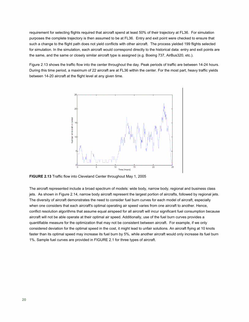
Figure 2.13 shows the traffic flow into the center throughout the day. Peak periods of traffic are between 14-24 hours. During this time period, a maximum of 22 aircraft are at FL36 within the center. For the most part, heavy traffic yields between 14-20 aircraft at the flight level at any given time.
FIGURE 2.13 Traffic flow into Cleveland Center throughout May 1, 2005
The aircraft represented include a broad spectrum of models: wide body, narrow body, regional and business class jets. As shown in Figure 2.14, narrow body aircraft represent the largest portion of aircrafts, followed by regional jets. The diversity of aircraft demonstrates the need to consider fuel burn curves for each model of aircraft, especially when one considers that each aircraft's optimal operating air speed varies from one aircraft to another. Hence, conflict resolution algorithms that assume equal airspeed for all aircraft will incur significant fuel consumption because aircraft will not be able operate at their optimal air speed. Additionally, use of the fuel burn curves provides a quantifiable measure for the optimization that may not be consistent between aircraft. For example, if we only considered deviation for the optimal speed in the cost, it might lead to unfair solutions. An aircraft flying at 10 knots faster than its optimal speed may increase its fuel burn by 5%, while another aircraft would only increase its fuel burn 1%. Sample fuel curves are provided in FIGURE 2.1 for three types of aircraft.
20
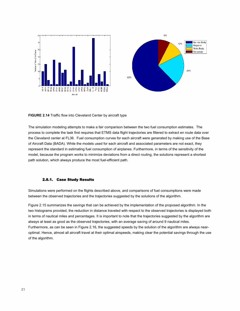
FIGURE 2.14 Traffic flow into Cleveland Center by aircraft type
The simulation modeling attempts to make a fair comparison between the two fuel consumption estimates. The process to complete the task first requires that ETMS data flight trajectories are filtered to extract en route data over the Cleveland center at FL36. Fuel consumption curves for each aircraft were generated by making use of the Base of Aircraft Data (BADA). While the models used for each aircraft and associated parameters are not exact, they represent the standard in estimating fuel consumption of airplanes. Furthermore, in terms of the sensitivity of the model, because the program works to minimize deviations from a direct routing, the solutions represent a shortest path solution, which always produce the most fuel-efficient path.
2.8.1. Case Study Results
Simulations were performed on the flights described above, and comparisons of fuel consumptions were made between the observed trajectories and the trajectories suggested by the solutions of the algorithm.
Figure 2.15 summarizes the savings that can be achieved by the implementation of the proposed algorithm. In the two histograms provided, the reduction in distance traveled with respect to the observed trajectories is displayed both in terms of nautical miles and percentages. It is important to note that the trajectories suggested by the algorithm are always at least as good as the observed trajectories, with an average saving of around 9 nautical miles. Furthermore, as can be seen in Figure 2.16, the suggested speeds by the solution of the algorithm are always near-optimal. Hence, almost all aircraft travel at their optimal airspeeds, making clear the potential savings through the use of the algorithm.
21
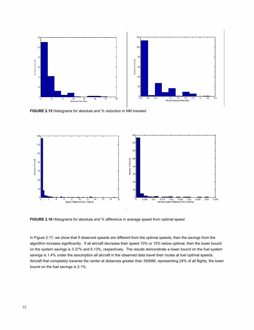
FIGURE 2.15 Histograms for absolute and % reduction in NM traveled
FIGURE 2.16 Histograms for absolute and % difference in average speed from optimal speed
In Figure 2.17, we show that if observed speeds are different from the optimal speeds, then the savings from the algorithm increase significantly. If all aircraft decrease their speed 10% or 15% below optimal, then the lower bound on the system savings is 3.37% and 6.13%, respectively. The results demonstrate a lower bound on the fuel system savings is 1.4% under the assumption all aircraft in the observed data travel their routes at fuel optimal speeds. Aircraft that completely traverse the center at distances greater than 350NM, representing 24% of all flights, the lower bound on the fuel savings is 2.1%.
22
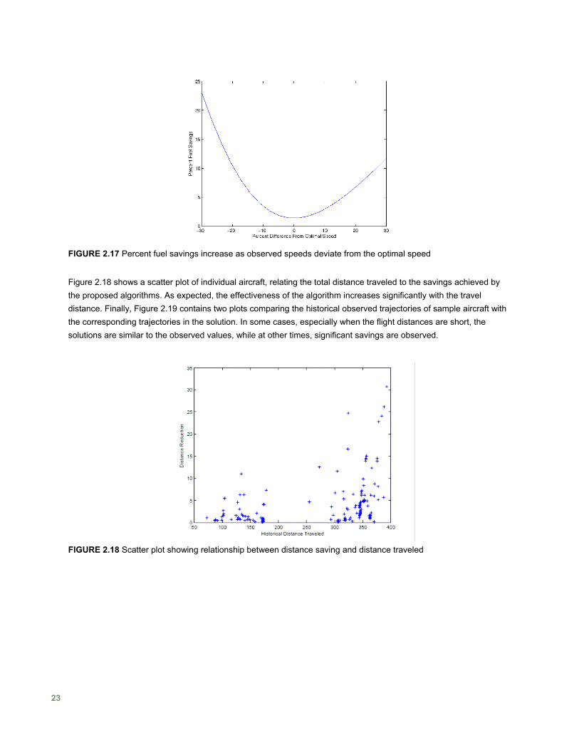
FIGURE 2.17 Percent fuel savings increase as observed speeds deviate from the optimal speed
Figure 2.18 shows a scatter plot of individual aircraft, relating the total distance traveled to the savings achieved by the proposed algorithms. As expected, the effectiveness of the algorithm increases significantly with the travel distance. Finally, Figure 2.19 contains two plots comparing the historical observed trajectories of sample aircraft with the corresponding trajectories in the solution. In some cases, especially when the flight distances are short, the solutions are similar to the observed values, while at other times, significant savings are observed.
FIGURE 2.18 Scatter plot showing relationship between distance saving and distance traveled
23
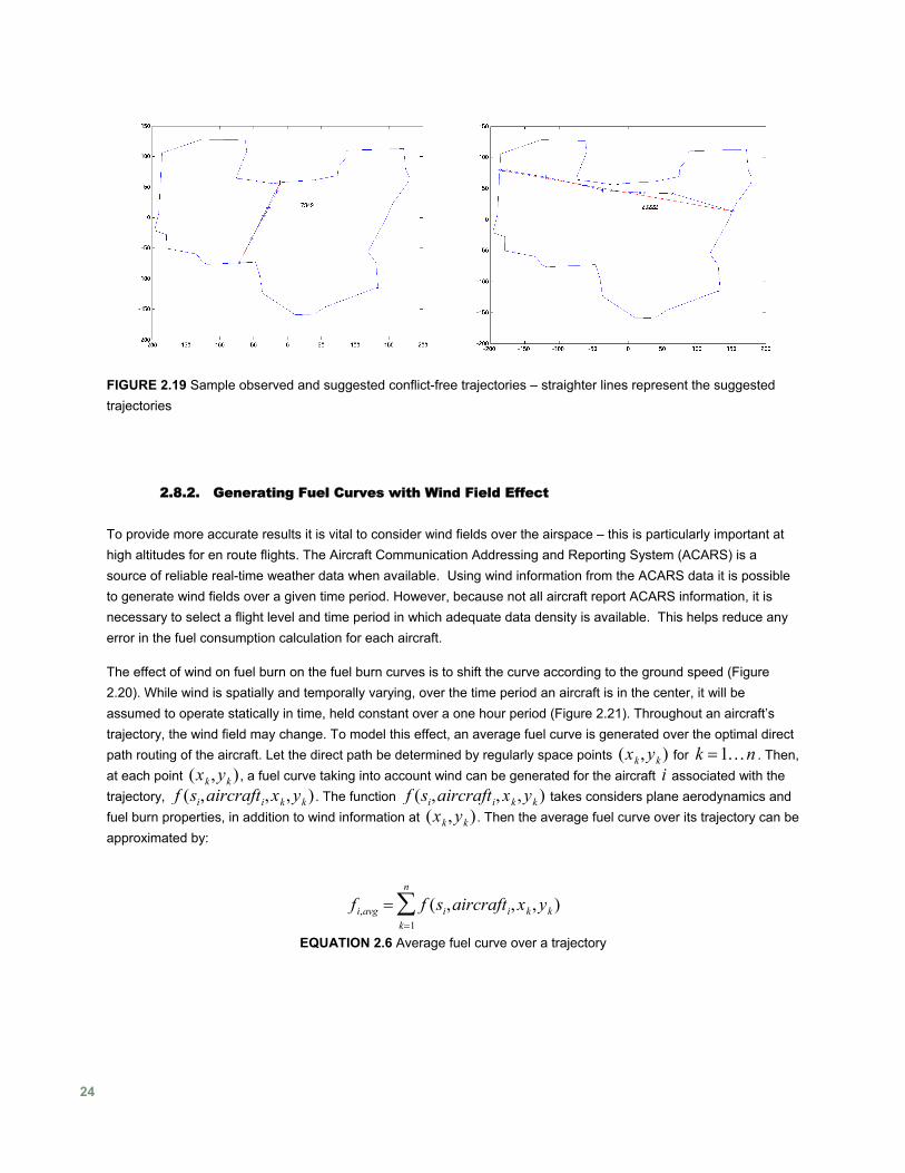
FIGURE 2.19 Sample observed and suggested conflict-free trajectories – straighter lines represent the suggested trajectories
2.8.2. Generating Fuel Curves with Wind Field Effect
To provide more accurate results it is vital to consider wind fields over the airspace – this is particularly important at high altitudes for en route flights. The Aircraft Communication Addressing and Reporting System (ACARS) is a source of reliable real-time weather data when available. Using wind information from the ACARS data it is possible to generate wind fields over a given time period. However, because not all aircraft report ACARS information, it is necessary to select a flight level and time period in which adequate data density is available. This helps reduce any error in the fuel consumption calculation for each aircraft.
The effect of wind on fuel burn on the fuel burn curves is to shift the curve according to the ground speed (Figure 2.20). While wind is spatially and temporally varying, over the time period an aircraft is in the center, it will be assumed to operate statically in time, held constant over a one hour period (Figure 2.21). Throughout an aircraft’s trajectory, the wind field may change. To model this effect, an average fuel curve is generated over the optimal direct path routing of the aircraft. Let the direct path be determined by regularly space points (xk , yk ) for . Then, at each point (
k =1Knxk , yk ), a fuel curve taking into account wind can be generated for the aircraft i associated with the
trajectory, f (si,aircrafti, xk , yk ) . The function f (si,aircrafti, xk , yk ) takes considers plane aerodynamics and fuel burn properties, in addition to wind information at (xk , yk ). Then the average fuel curve over its trajectory can be approximated by:
fi,avg = f (si,aircrafti,xk ,yk )k=1
n
∑
EQUATION 2.6 Average fuel curve over a trajectory
24
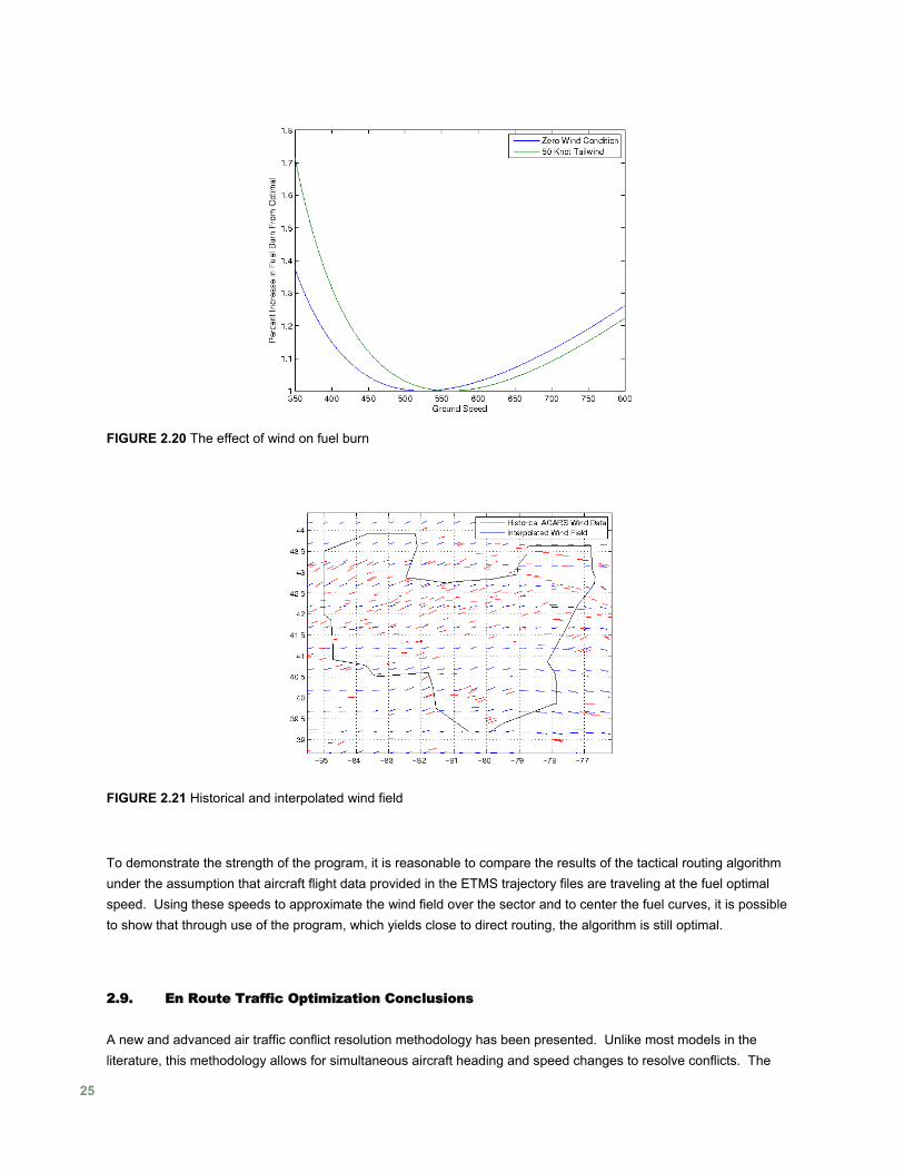
FIGURE 2.20 The effect of wind on fuel burn
FIGURE 2.21 Historical and interpolated wind field
To demonstrate the strength of the program, it is reasonable to compare the results of the tactical routing algorithm under the assumption that aircraft flight data provided in the ETMS trajectory files are traveling at the fuel optimal speed. Using these speeds to approximate the wind field over the sector and to center the fuel curves, it is possible to show that through use of the program, which yields close to direct routing, the algorithm is still optimal.
2.9. En Route Traffic Optimization Conclusions
A new and advanced air traffic conflict resolution methodology has been presented. Unlike most models in the literature, this methodology allows for simultaneous aircraft heading and speed changes to resolve conflicts. The
25

maneuvers are determined such that the fuel costs incurred due to the changes are minimized. The nonconvex cost functions of airspeeds and headings have been modeled using linear approximations, which lead to very accurate representations of the actual cost functions. A significant characteristic of the proposed approach is that the optimal conflict resolution maneuvers are identified in only a few seconds, which enables implementation of the developed methodology in real-time traffic flow management.
The simulations performed similar to a near-real time implementation in a receding horizon format demonstrate the ability for the proposed method to effectively deconflict and route aircraft through an airspace while reducing fuel consumption for aircraft over current methods. While some improvement margins are small, they clearly demonstrate an overall improvement.
Future work considered is for the developed procedure to be extended to three dimensions by modeling multiple flight levels, and introducing new variables in the mixed integer programming formulation to represent allowable movements between these levels. This extension is important and will especially add value to the described approach, given the additional flexibility to be gained to resolve conflicts. Also, additional work will focus on routing aircraft along non-direct routes. Focusing on non-direct routing will allow for a conflict resolution algorithm to take into consideration inclement weather and more complex wind fields. Furthermore, the model can be compared with existing heuristic procedures, and the results from the fully implemented optimization procedure can be used as a baseline in evaluating other proposed methods. In addition, computational performance for instances involving a very large number of aircraft can be improved by using different parallelization schemes and advanced integer programming solution techniques.
26
3. En Route Speed Change Optimization for Continuous Descent Arrivals
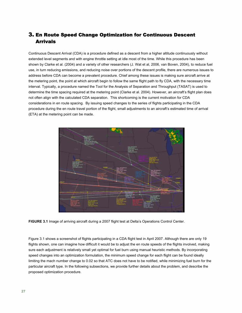
Continuous Descent Arrival (CDA) is a procedure defined as a descent from a higher altitude continuously without extended level segments and with engine throttle setting at idle most of the time. While this procedure has been shown by Clarke et al. (2004) and a variety of other researchers (J. Wat et al, 2006, van Boven, 2004), to reduce fuel use, in turn reducing emissions, and reducing noise over portions of the descent profile, there are numerous issues to address before CDA can become a prevalent procedure. Chief among these issues is making sure aircraft arrive at the metering point, the point at which aircraft begin to follow the same flight path to fly CDA, with the necessary time interval. Typically, a procedure named the Tool for the Analysis of Separation and Throughput (TASAT) is used to determine the time spacing required at the metering point (Clarke et al. 2004). However, an aircraft’s flight plan does not often align with the calculated CDA separation. This shortcoming is the current motivation for CDA considerations in en route spacing. By issuing speed changes to the series of flights participating in the CDA procedure during the en route travel portion of the flight, small adjustments to an aircraft’s estimated time of arrival (ETA) at the metering point can be made.
FIGURE 3.1 Image of arriving aircraft during a 2007 flight test at Delta’s Operations Control Center.
Figure 3.1 shows a screenshot of flights participating in a CDA flight test in April 2007. Although there are only 19 flights shown, one can imagine how difficult it would be to adjust the en route speeds of the flights involved, making sure each adjustment is relatively small yet optimal for fuel burn using manual heuristic methods. By incorporating speed changes into an optimization formulation, the minimum speed change for each flight can be found ideally limiting the mach number change to 0.02 so that ATC does not have to be notified, while minimizing fuel burn for the particular aircraft type. In the following subsections, we provide further details about the problem, and describe the proposed optimization procedure.
27
3.1. State of the Art Limitations
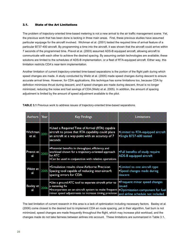
The problem of trajectory-oriented time-based metering is not a new arrival to the air traffic management scene. Yet, the previous work that has been done is lacking in three main areas. First, these previous studies have assumed particular equipage for the aircraft involved. Wichman et al. (2001) tested the required time of arrival feature of a particular B737-400 aircraft. By programming a time into the aircraft, it was shown that the aircraft could arrive within 7 seconds of the programmed time. Prevot et al. (2003) assumed ADS-B equipped aircraft, allowing aircraft to communicate with each other to achieve the desired spacing. By assuming certain technologies are available; these solutions are limited to the schedules of ADS-B implementation, or a fleet of RTA-equipped aircraft. Either way, this limitation restricts CDA’s near-term implementation.
Another limitation of current trajectory-oriented time-based separations is the portion of the flight path during which speed changes are made. A study conducted by Weitz et al. (2005) made speed changes during descent to ensure accurate arrival times. However, for CDA applications, this technique has some limitations too, because CDA by definition minimizes thrust during descent, and if speed changes are made during descent, thrust is no longer minimized, reducing the noise and fuel savings of CDA (Weitz et al. 2005). In addition, the amount of spacing adjustment is limited by the amount of speed adjustment available to the pilot.
TABLE 3.1 Previous work to address issues of trajectory-oriented time-based separations.
The last limitation of current research in this area is a lack of optimization including necessary factors. Baxley et al. (2006) come closest to the desired tool to implement CDA en route spacing, yet in their algorithm, fuel burn is not minimized, speed changes are made frequently throughout the flight, which may increase pilot workload, and the changes made do not take fairness between airlines into account. These limitations are summarized in Table 3.1.
28
With the background for CDA en route considerations set, and the limitations in current solutions, the goals of en route spacing to implement CDA are as follows:
• Capable of implementation for a variety of aircraft • Does not assume ADS-B equipage (near-term implementation) • Minimum number of speed changes made to limit the workload for the flight crew • Speed changes should be optimized to limit the increase in fuel burn • Speed changes should not favor one airline over another, i.e. include fairness considerations • Automate the optimization process as much as possible
Consideration of fairness is necessary to any implementation of CDA, as both pilots and airlines must agree to perform the procedure. If each party acknowledges and accepts that fuel burn and scheduling of participating flights are altered as fairly as possible, it is assumed that parties will be willing to participate. For this problem, fairness is defined as the allocation of speed changes that ensure a proportional (divided in proportion to the claimant’s contribution), envy-free (each claimant satisfied with his share), equitable (all parties thinking they received the same portion of the total), efficient (Pareto efficiency), and truthful (one party cannot lie about the facts determining their resource allocation) measuring and allocation of additional fuel used per airline. Further explanations of these fairness descriptions can be found in the Brams and Taylor references and in Section 3.3.3. The ensuing subsections describe how these goals have been met.
3.2. En Route Speed Alteration Formulations
While developing a computer program to meet the previously mentioned performance goals, several iterations of algorithms were developed. Each of the formulations, a one-speed change formulation, a two-speed change formulation, and variations of those two formulations including fairness considerations, are described in this subsection.
3.2.1. One Speed-Change Formulation
The one-change formulation was developed in order to test the feasibility of the solution procedure and provide a baseline for future optimization results. In addition, the basic derivations of the one speed-change formulation hold for the ensuing two speed-change and two speed-change with fairness solutions. The first part of the equation is the cost function, which simply states that the fuel burn should be minimized for the entire aircraft fleet.
(3.1)
Following this equation are the necessary constraints on the objective function. It is first necessary to linearize the fuel burn curve for each aircraft involved in the CDA procedure. Performance data describing these fuel burn curves was provided through a partnership with Delta Air Lines. The aircraft involved in this sample CDA flight test for which the fuel burn data was collected were Boeing 767-400, 767-300, 757-200, and Boeing 737-800 aircraft. This process is equivalent to the following series of constraints:
29
(3.2a-2c)
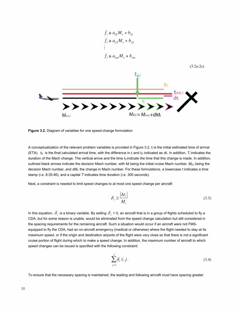
Figure 3.2. Diagram of variables for one speed-change formulation
A conceptualization of the relevant problem variables is provided in Figure 3.2. ti is the initial estimated time of arrival (ETA). tD is the final calculated arrival time, with the difference in ti and tD indicated as dti. In addition, Ti indicates the duration of the Mach change. The vertical arrow and the time t0 indicate the time that this change is made. In addition, outlined black arrows indicate the decision Mach number, with Mi being the initial cruise Mach number, MD,i being the decision Mach number, and dMi, the change in Mach number. For these formulations, a lowercase t indicates a time stamp (i.e. 8:35:46), and a capital T indicates time duration (i.e. 300 seconds).
Next, a constraint is needed to limit speed changes to at most one speed change per aircraft:
i
ii M
tΔ≥δ (3.3)
In this equation, iδ is a binary variable. By setting iδ = 0, an aircraft that is in a group of flights scheduled to fly a CDA, but for some reason is unable, would be eliminated from the speed change calculation but still considered in the spacing requirements for the remaining aircraft. Such a situation would occur if an aircraft were not FMS-equipped to fly the CDA, had an on-aircraft emergency (medical or otherwise) where the flight needed to stay at its maximum speed, or if the origin and destination airports of the flight were very close so that there is not a significant cruise portion of flight during which to make a speed change. In addition, the maximum number of aircraft to which speed changes can be issued is specified with the following constraint:
. (3.4) δi ≤ jj=1∑
J
To ensure that the necessary spacing is maintained, the leading and following aircraft must have spacing greater
30
than or equal to their TASAT-calculated1 separation:
(ti+1 − Δti+1) − (ti − Δti+1) ≥ Si,i+1. (3.5)
It is then necessary to relate the change in the estimated time of arrival (ETA) to the change in Mach number, assuming the change in velocity is much less than the cruise velocity, with winds considered. With these assumptions and a complete derivation explained in Appendix A, a relationship between time and Mach number can be derived:
Δti = TiΔMi
Mi
. (3.6)
Lastly, it is necessary to limit the possible change in Mach number and calculate the net time during which the speed change is made, the final (decision) Mach number, and the final ETA. These tasks are performed by the following three constraints:
ΔMi ≤ 0.02, (3.7)
Md iMi = − ΔMi , and (3.8)
t fiti ti . (3.9) = − Δ
3.2.2. One Speed Change Algorithm While Minimizing Initial and Final ETA Difference
The objective function, Equation 3.1 above, does not take into account the fact that if there is a speed change for each aircraft, the time duration during which the speed change occurs is no longer fixed. The previous objective function amounts to finding the speed change for each aircraft which brings it as close as possible to the aircraft’s maximum endurance cruise speed. While this objective function would seem to reduce the overall fuel burn, as explained by Abad (2004), “Further consider that the coupling between fuel burn and flight time is complex due to the occasional trade-off in optimizing for one at the expense of the other. This coupling is obvious when considering the causality of flight time upon fuel burn: a longer flight time necessitates a greater fuel burn”. This scenario is exactly the case in the present problem.
If the flights in question all had initial cruise speeds below the speed of minimum fuel burn rate, the above objective function, Equation 3.1, would be adequate. The flights would all increase speed by some amount so that they reach the required separation, the flights would arrive earlier, and fuel would be saved during the en route segment of the flight, as well as during the CDA. However, this is not the reality. Most flights during the 2007 flight test were cruising above the maximum endurance speed, close to the cruise speed for maximum range. Since this higher cruise speed was the observed scenario, the above objective function decreased the speed of each flight, actually resulting in increased fuel burn for each flight. With this result, the objective function was reexamined, and it was necessary to include the time change in the objective function as well. A simple addition to the above function is
( )∑=
⎟⎠⎞
⎜⎝⎛ Δ−=
N
iiiMi tTfZ
id1min & . (3.10)
1 Tool for Analysis of Separation and Throughput (TASAT) is a tool running simulations of various aircraft and wind conditions to find an optimal aircraft spacing. It is described in further detail by Clarke et al. 2004.
31
While this addition of t is straightforward in terms of logic, the resulting math is not as simple. Including two unknowns in the objective function when multiplied, create a nonconvex problem. Fortunately, the problem has been encountered previously, and Babayev (1997) has provided a way to deal with such a situation by adding additional constraints.
The approximation method is equivalent to creating a new variable which replaces the nonlinear terms,
iMi tfrid
Δ= & . (3.11)
The following approximations create a series of planes outlining the values of the function. It is then necessary to create a grid for the possible values of ri. These grid points are denoted by
λkli≈ FkΔTl (3.12)
with each being a grid point for a specific ri value. The remaining constraints for this approximation are then
i
idkl
k lkM
Ff λ∑∑=& (3.13)
Δti = ΔTll
∑k
∑ λkli (3.14)
ri = FkΔTl( )l
∑k
∑ λkli (3.15)
λkli=1
l∑
k∑ (3.16)
μki= λkli
l∑ (3.17)
ηli= λkli
k∑ (3.18)
≥ 0 (3.19) λkli
SOS2 (3.20) μki∈
SOS2 (3.21) ηli∈
ri free . (3.22) →
In the above equations, k and l are the number of grid points in the fuel burn and time ranges respectively. In this case, the range of possible fuel burn rate values is needed, as well as the range of t’s. In order to keep the
32
calculation capable of being solved in a reasonable amount of time, a small range of t’s are used. It is assumed that the maximum range for t is within ten minutes of the original ETA, meaning the range of t is -300 seconds < t < 300 seconds. The range of
idMf& is from the lowest possible fuel burn rate for which there is data to the highest fuel burn
rate for which there is data for all aircraft types. By summing these grid values, and enforcing the condition that at most four adjacent weights are nonzero (by SOS2 variables), the appropriate portion of the function can be approximated.
3.2.3. Fairness Considerations in Speed Alteration Algorithms
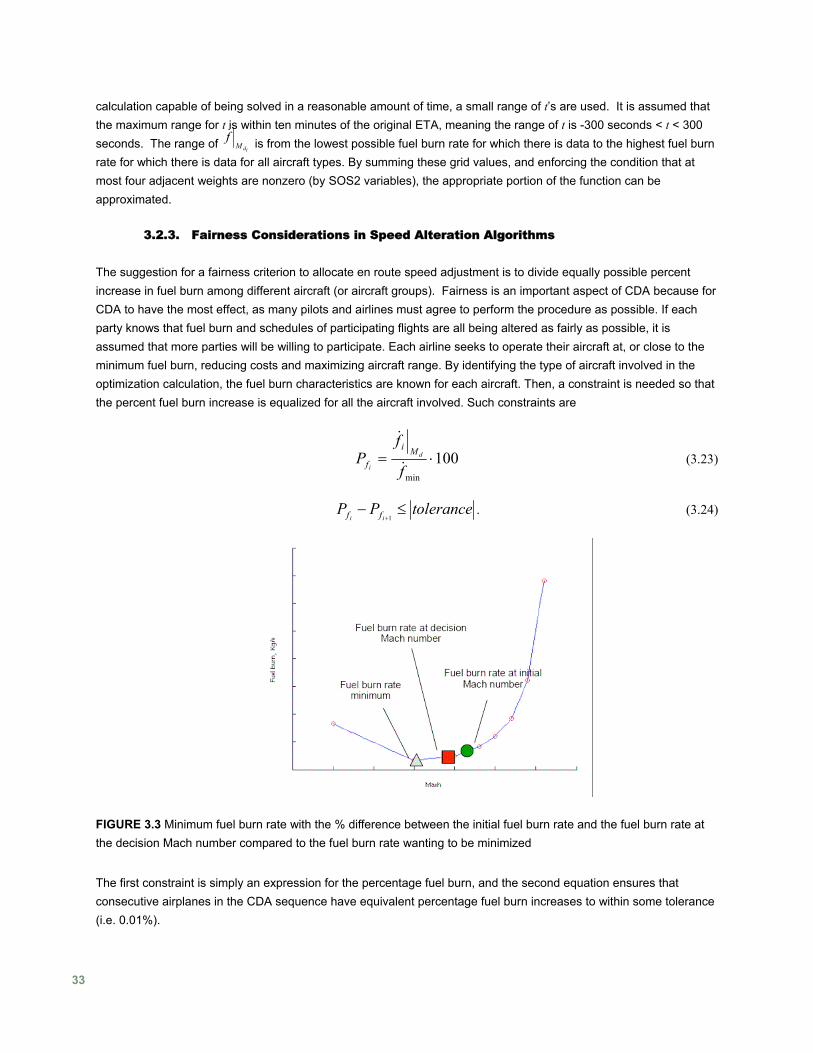
The suggestion for a fairness criterion to allocate en route speed adjustment is to divide equally possible percent increase in fuel burn among different aircraft (or aircraft groups). Fairness is an important aspect of CDA because for CDA to have the most effect, as many pilots and airlines must agree to perform the procedure as possible. If each party knows that fuel burn and schedules of participating flights are all being altered as fairly as possible, it is assumed that more parties will be willing to participate. Each airline seeks to operate their aircraft at, or close to the minimum fuel burn, reducing costs and maximizing aircraft range. By identifying the type of aircraft involved in the optimization calculation, the fuel burn characteristics are known for each aircraft. Then, a constraint is needed so that the percent fuel burn increase is equalized for all the aircraft involved. Such constraints are
100min
⋅=f
fP d
i
Mi
f &
&
(3.23)
PfiPfi+1
tolerance . (3.24) − ≤
FIGURE 3.3 Minimum fuel burn rate with the % difference between the initial fuel burn rate and the fuel burn rate at the decision Mach number compared to the fuel burn rate wanting to be minimized
The first constraint is simply an expression for the percentage fuel burn, and the second equation ensures that consecutive airplanes in the CDA sequence have equivalent percentage fuel burn increases to within some tolerance (i.e. 0.01%).
33
An example fuel burn curve is shown in Figure 3.3. The highlighted area shows an example of a range of possible values, centering on the initial cruise Mach of the aircraft (indicated by the circle). The percentage deviation from the triangle, the fuel burn minimum to the square will be equalized for each flight in the CDA-performing fleet. These constraints are a part of the optimization model so that each aircraft has the same percentage increase in fuel burn for their re-routings.
3.2.4. Variable Sequence Constraints
It was initially thought that keeping a fixed sequence of aircraft, based on the initial ETA’s of the aircraft group, would help to simplify the optimization problem. Such was the assumption explained in Equation 3.5. By keeping a fixed sequence, it is only necessary to know the required separation between pairs of leading and following aircraft. These n-1 constraints are easy to work with, and minimal coordination with TASAT is necessary, since only a few combinations of leading and following aircraft are needed.
However, by freezing the sequence of the aircraft, the many combinations of aircraft ordering are ignored, and the solution giving the lowest possible increase in fuel burn may be missed entirely. In addition, for terminal area landing scenarios where there is limited time to set up aircraft with a necessary separation, enabling a variable sequence in the formulation is even more important. The easiest way to see how a series of variable sequence constraints can be implemented can be seen by examining just three aircraft. For three aircraft, one sets a separation distance between all three for each leading and following scenario. The conditions to be satisfied are:
TSC1− TSC2
≥ α1,2 (3.25)
TSC1− TSC3
≥ α1,3 (3.26)
TSC2− TSC3
≥ α2,3, (3.27)
with alpha being the required separation distance based on aircraft type. Here, the separation time is written as being the same regardless of the aircraft order, but there will be a different αi,i value depending on the order of the aircraft. For example, the separation time for a B767-300 following a B737-800 would be significant lower than for the case where the B737-800 follows the B767-300, due to the size difference of the aircraft. However, absolute values create a non-convex problem and these constraints must be rewritten as
T2 − T1 + α1,2 ≤ Pz1 (3.28)
2α2,1 − (T2 T1 P z )1 (3.29) ) (1− + α2,1 ≤ −
T3 T1− + α1,3 ≤ Pz
2
2 (3.30)
α3,1 − (T3 T1 P z )2 (3.31) ) (1− + α3,1 ≤ −
T3 T2− + α2,3 ≤ Pz
2
3 (3.32)
α3,2 − (T3 T2 P z )3 , (3.33) ) (1− + α3,2 ≤ −
where z1, z2, and z3 are binary variables, and P is sufficiently large so that one constraint is made invalid. In addition,
34
the different separation time for the reciprocal aircraft orders are indicated by αi,j and αj,i for each pair of constraints. Only one separation constraint will be active because of the binary variables and large value of P.
For multiple aircraft, determining all possible combinations of orders and the necessary separation adds many constraints, but does not change the solution time of the problem significantly. For n aircraft, it is necessary to have
constraints (3 aircraft necessitates 6 constraints, 5 aircraft necessitates 15 constraints, 16 aircraft necessitates 120 constraints, etc.). ∑
N
i1
3.3. Computational Study for the En Route Spacing Program
In this section, we describe the computational tests conducted. The following assumptions were used in the implementation of the models:
• The earliest possible time for a speed change is two hours prior to arrival at the metering point • All aircraft in the simulation are able to make a speed change (this can be adjusted in actual flight tests
for nonparticipating aircraft) • The tolerance for fairness equalization is 0.0001 (expressed as a decimal, not a percentage) • It is assumed that discrete Mach number changes can be made with thousandth accuracy (i.e. increase
Mach 0.005). Although this is not a hard constraint in the results presented, it is assumed that rounding to this accuracy will not affect the calculation results
• In order to ensure the Mach change is allowable by ATC, the maximum possible deviation in Mach is 0.02.
• Participating aircraft types are limited to Boeing 767-400, 767-300, 757-200, and 737-800 aircraft, as those were the only aircraft types flown by Delta during this flight test. The fuel burn data was obtained through a Non Disclosure Agreement with Boeing Aircraft. (The algorithm can handle other aircraft types; so long as the fuel burn information is obtained ahead of time from the aircraft manufacturer.)
3.3.1. Sample CDA Flight Test Case
During the April-May 2007 flight test, CDA operations were observed for a period of 4 weeks. During this time, 31 days of flights flying early morning operations from the west coast were observed to fly a CDA path shown in the figure below. While the fuel savings and noise data are still currently unavailable for these flights, this flight scenario provides a range of sample scenarios for late night CDA operations. A range of aircraft—B737-800, B757-200, B767-300, and B767-400—were involved in the flight tests, as well as a range of wind conditions for each night. The information collected from each day’s flight test was the date, flight number, tail number, origin airport of the flight, whether the plane flew the CDA or not, the runway to which the flight was directed, cruising altitude, cruising Mach, takeoff weight, required time of arrival at the metering point RMG, the actual time of arrival at RMG, the scheduled arrival time for the destination (ATL), the ATA at ATL, and wheels on time at ATL.
With this information, cases mirroring what was observed could be tested using the spacing tool developed, En route Speed Change Optimization Relay Tool (ESCORT). On one day, due to the tight initial spacing of the flights (among other factors not recorded), 10 of the 16 flights were unable to fly the CDA. A key usefulness test for this study is to show the ease with which ESCORT provides a solution to previous problems encountered, and also to show that more complex scenarios than what has currently been observed can also be handled. On this sample, worst-case scenario day, there were 15 flights, all scheduled to arrive over the metering point RMG, between 9:06 AM and 11:40 AM. While on that night, care was taken to space these flights as well as possible, there were too many factors to take into account during a live flight test. With such tight groupings, knowing how to increase and decrease the speeds of the flights without creating new separation conflicts was beyond the capacity of myself and the other flight test researchers present. While this day shows the limitation of heuristic approaches to spacing, it also provides a scenario to showcase ESCORT’s usefulness. The details of the difficult May 22, 2007 scenario that will be the basis
35
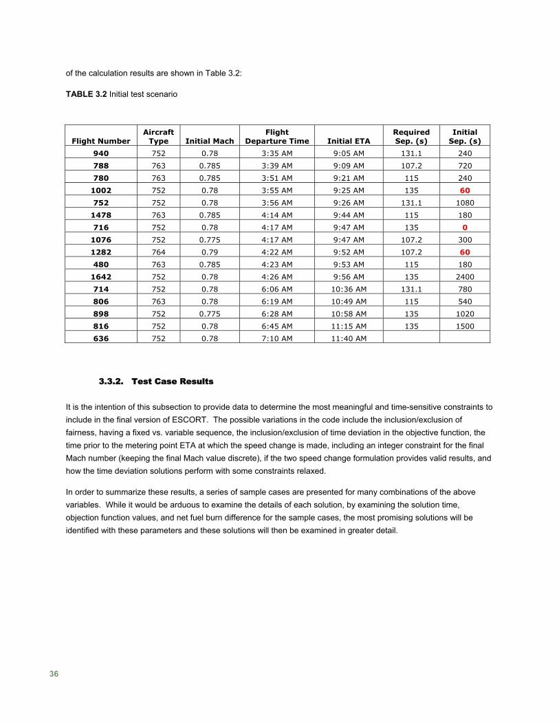
of the calculation results are shown in Table 3.2:
TABLE 3.2 Initial test scenario
Flight Number Aircraft
Type Initial Mach Flight
Departure Time Initial ETA Required Sep. (s)
Initial Sep. (s)
940 752 0.78 3:35 AM 9:05 AM 131.1 240
788 763 0.785 3:39 AM 9:09 AM 107.2 720
780 763 0.785 3:51 AM 9:21 AM 115 240
1002 752 0.78 3:55 AM 9:25 AM 135 60
752 752 0.78 3:56 AM 9:26 AM 131.1 1080
1478 763 0.785 4:14 AM 9:44 AM 115 180
716 752 0.78 4:17 AM 9:47 AM 135 0
1076 752 0.775 4:17 AM 9:47 AM 107.2 300
1282 764 0.79 4:22 AM 9:52 AM 107.2 60
480 763 0.785 4:23 AM 9:53 AM 115 180
1642 752 0.78 4:26 AM 9:56 AM 135 2400
714 752 0.78 6:06 AM 10:36 AM 131.1 780
806 763 0.78 6:19 AM 10:49 AM 115 540
898 752 0.775 6:28 AM 10:58 AM 135 1020
816 752 0.78 6:45 AM 11:15 AM 135 1500
636 752 0.78 7:10 AM 11:40 AM
3.3.2. Test Case Results
It is the intention of this subsection to provide data to determine the most meaningful and time-sensitive constraints to include in the final version of ESCORT. The possible variations in the code include the inclusion/exclusion of fairness, having a fixed vs. variable sequence, the inclusion/exclusion of time deviation in the objective function, the time prior to the metering point ETA at which the speed change is made, including an integer constraint for the final Mach number (keeping the final Mach value discrete), if the two speed change formulation provides valid results, and how the time deviation solutions perform with some constraints relaxed.
In order to summarize these results, a series of sample cases are presented for many combinations of the above variables. While it would be arduous to examine the details of each solution, by examining the solution time, objection function values, and net fuel burn difference for the sample cases, the most promising solutions will be identified with these parameters and these solutions will then be examined in greater detail.
36
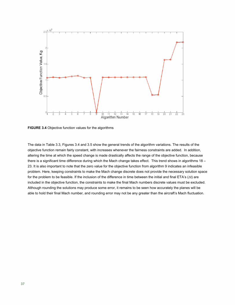
FIGURE 3.4 Objective function values for the algorithms
The data in Table 3.3, Figures 3.4 and 3.5 show the general trends of the algorithm variations. The results of the objective function remain fairly constant, with increases whenever the fairness constraints are added. In addition, altering the time at which the speed change is made drastically affects the range of the objective function, because there is a significant time difference during which the Mach change takes effect. This trend shows in algorithms 18 – 23. It is also important to note that the zero value for the objective function from algorithm 9 indicates an infeasible problem. Here, keeping constraints to make the Mach change discrete does not provide the necessary solution space for the problem to be feasible. If the inclusion of the difference in time between the initial and final ETA’s (Δt) are included in the objective function, the constraints to make the final Mach numbers discrete values must be excluded. Although rounding the solutions may produce some error, it remains to be seen how accurately the planes will be able to hold their final Mach number, and rounding error may not be any greater than the aircraft’s Mach fluctuation.
37

FIGURE 3.5 Run time and fuel burn differences for the algorithms
Other general trends include a drastic increase in run time with increasing numbers of grid points for the Δt inclusion. The outlying point in the run time results corresponds to selecting 6 grid points for the Δt inclusion. While a finer grid results in an increased fuel savings (~3 kg), the run time of nearly 2 hrs makes grids with an increased resolution difficult to run the program in real time. However, it is assumed that increased computing power will decrease these solution times. The calculations were made on a computer with a quad-core 2 GHz processor.
Because the motivation for this research is primarily an environmental one, with projected goals of fuel savings and reduced costs/emissions via this reduction, the algorithm which gives results with the lowest net fuel burn increase and solving in a reasonable amount of time, will be considered the best. It would be tempting to simply use the algorithm which gives the minimum objective function, in this case Algorithm 1. However, although this is the lowest objective value, it was mentioned previously that this algorithm does not take into account the added travel time in the calculation of its objective function. By using the lowest net fuel burn increase as the utility measure, the analyst avoids falling into this trap.
The net fuel burn displayed in Figure 3.5 is the sum of the fuel burn difference for each aircraft compared to the fuel burned had the aircraft remained at its initial cruise Mach. It is interesting to note that several of the algorithms result in a net fuel savings for the en route portion of the flight, and this fuel savings is independent of the CDA benefits, which have yet to be taken into account. While the fuel savings is modest (~10 kg per aircraft), due to the concern that CDA spacing may induce greater fuel burn before descent, this may not necessarily be the case.
38
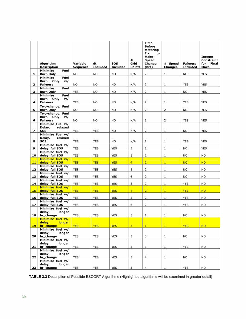
Algorithm Description
Variable Sequence
dt Included
SOS Included
# Grid Points
Time Before Metering Fix to Make Speed Change (hrs)
# Speed Changes
Fairness Included
Integer Constraint for Final Mach
1 Minimize Fuel Burn Only NO NO NO N/A 2 1 NO YES
2
Minimize Fuel Burn Only w/ Fairness NO NO NO N/A 2 1 YES YES
3 Minimize Fuel Burn Only YES NO NO N/A 2 1 NO YES
4
Minimize Fuel Burn Only w/ Fairness YES NO NO N/A 2 1 YES YES
5 Two-change, Fuel Burn Only NO NO NO N/A 2 2 NO YES
6
Two-change, Fuel Burn Only w/ Fairness NO NO NO N/A 2 2 YES YES
7
Minimize Fuel w/ Delay, relaxed SOS YES YES NO N/A 2 1 NO YES
8
Minimize Fuel w/ Delay, relaxed SOS YES YES NO N/A 2 1 YES YES
9 Minimize fuel w/ delay, full SOS YES YES YES 3 2 1 NO YES
10 Minimize fuel w/ delay, full SOS YES YES YES 3 2 1 NO NO
11 Minimize fuel w/ delay, full SOS YES YES YES 4 2 1 NO NO
12 Minimize fuel w/ delay, full SOS YES YES YES 5 2 1 NO NO
13 Minimize fuel w/ delay, full SOS YES YES YES 6 2 1 NO NO
14 Minimize fuel w/ delay, full SOS YES YES YES 3 2 1 YES NO
15 Minimize fuel w/ delay, full SOS YES YES YES 4 2 1 YES NO
16 Minimize fuel w/ delay, full SOS YES YES YES 5 2 1 YES NO
17 Minimize fuel w/ delay, full SOS YES YES YES 6 2 1 YES NO
18
Minimize fuel w/ delay, longer hr_change YES YES YES 3 1 1 NO NO
19
Minimize fuel w/ delay, longer hr_change YES YES YES 3 1 1 YES NO
20
Minimize fuel w/ delay, longer hr_change YES YES YES 3 3 1 NO NO
21
Minimize fuel w/ delay, longer hr_change YES YES YES 3 3 1 YES NO
22
Minimize fuel w/ delay, longer hr_change YES YES YES 3 4 1 NO NO
23
Minimize fuel w/ delay, longer hr_change YES YES YES 3 4 1 YES NO
TABLE 3.3 Description of Possible ESCORT Algorithms (Highlighted algorithms will be examined in greater detail)
39
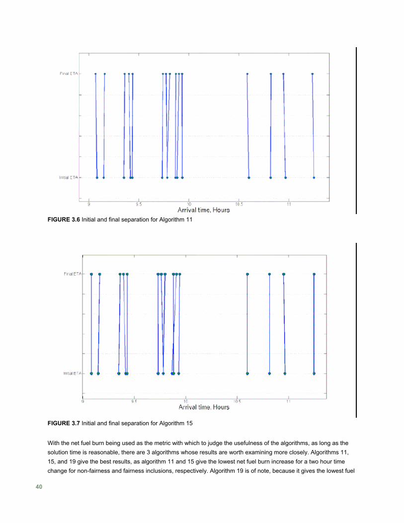
FIGURE 3.6 Initial and final separation for Algorithm 11
FIGURE 3.7 Initial and final separation for Algorithm 15
With the net fuel burn being used as the metric with which to judge the usefulness of the algorithms, as long as the solution time is reasonable, there are 3 algorithms whose results are worth examining more closely. Algorithms 11, 15, and 19 give the best results, as algorithm 11 and 15 give the lowest net fuel burn increase for a two hour time change for non-fairness and fairness inclusions, respectively. Algorithm 19 is of note, because it gives the lowest fuel
40
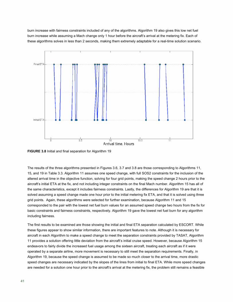
burn increase with fairness constraints included of any of the algorithms. Algorithm 19 also gives this low net fuel burn increase while assuming a Mach change only 1 hour before the aircraft’s arrival at the metering fix. Each of these algorithms solves in less than 2 seconds, making them extremely adaptable for a real-time solution scenario.
FIGURE 3.8 Initial and final separation for Algorithm 19
The results of the three algorithms presented in Figures 3.6, 3.7 and 3.8 are those corresponding to Algorithms 11, 15, and 19 in Table 3.3. Algorithm 11 assumes one speed change, with full SOS2 constraints for the inclusion of the altered arrival time in the objective function, solving for four grid points, making the speed change 2 hours prior to the aircraft’s initial ETA at the fix, and not including integer constraints on the final Mach number. Algorithm 15 has all of the same characteristics, except it includes fairness constraints. Lastly, the differences for Algorithm 19 are that it is solved assuming a speed change made one hour prior to the initial metering fix ETA, and that it is solved using three grid points. Again, these algorithms were selected for further examination, because Algorithm 11 and 15 corresponded to the pair with the lowest net fuel burn values for an assumed speed change two hours from the fix for basic constraints and fairness constraints, respectively. Algorithm 19 gave the lowest net fuel burn for any algorithm including fairness.
The first results to be examined are those showing the initial and final ETA separation calculated by ESCORT. While these figures appear to show similar information, there are important features to note. Although it is necessary for aircraft in each Algorithm to make a speed change to meet the separation constraints provided by TASAT, Algorithm 11 provides a solution offering little deviation from the aircraft’s initial cruise speed. However, because Algorithm 15 endeavors to fairly divide the increased fuel usage among the sixteen aircraft, treating each aircraft as if it were operated by a separate airline, more movement is necessary to still meet the separation requirements. Finally, in Algorithm 19, because the speed change is assumed to be made so much closer to the arrival time, more drastic speed changes are necessary indicated by the slopes of the lines from initial to final ETA. While more speed changes are needed for a solution one hour prior to the aircraft’s arrival at the metering fix, the problem still remains a feasible
41
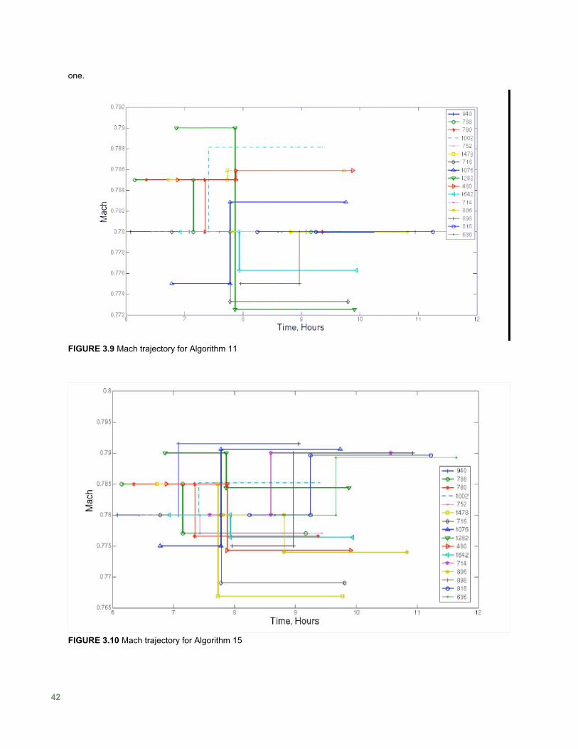
one.
FIGURE 3.9 Mach trajectory for Algorithm 11
FIGURE 3.10 Mach trajectory for Algorithm 15
42
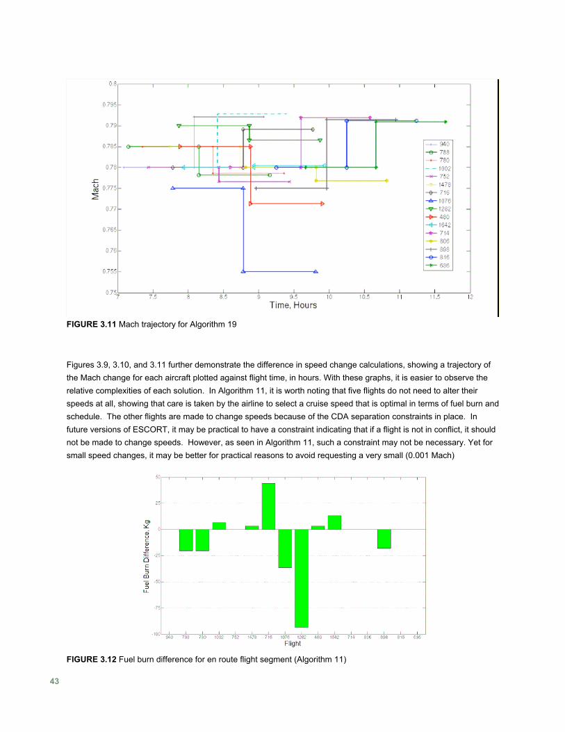
FIGURE 3.11 Mach trajectory for Algorithm 19
Figures 3.9, 3.10, and 3.11 further demonstrate the difference in speed change calculations, showing a trajectory of the Mach change for each aircraft plotted against flight time, in hours. With these graphs, it is easier to observe the relative complexities of each solution. In Algorithm 11, it is worth noting that five flights do not need to alter their speeds at all, showing that care is taken by the airline to select a cruise speed that is optimal in terms of fuel burn and schedule. The other flights are made to change speeds because of the CDA separation constraints in place. In future versions of ESCORT, it may be practical to have a constraint indicating that if a flight is not in conflict, it should not be made to change speeds. However, as seen in Algorithm 11, such a constraint may not be necessary. Yet for small speed changes, it may be better for practical reasons to avoid requesting a very small (0.001 Mach)
FIGURE 3.12 Fuel burn difference for en route flight segment (Algorithm 11)
43
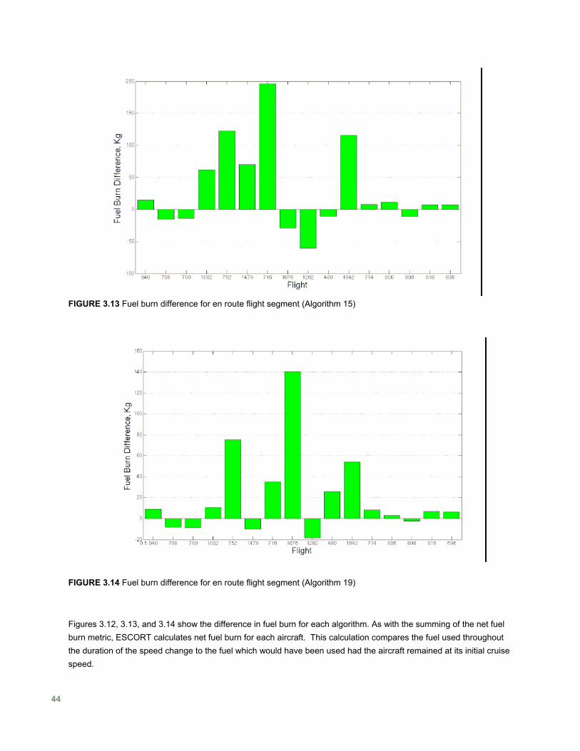
FIGURE 3.13 Fuel burn difference for en route flight segment (Algorithm 15)
FIGURE 3.14 Fuel burn difference for en route flight segment (Algorithm 19)
Figures 3.12, 3.13, and 3.14 show the difference in fuel burn for each algorithm. As with the summing of the net fuel burn metric, ESCORT calculates net fuel burn for each aircraft. This calculation compares the fuel used throughout the duration of the speed change to the fuel which would have been used had the aircraft remained at its initial cruise speed.
44
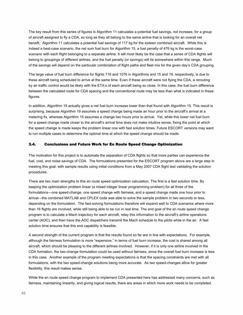
The key result from this series of figures is Algorithm 11 calculates a potential fuel savings, not increase, for a group of aircraft assigned to fly a CDA, so long as they all belong to the same airline that is looking for an overall net benefit. Algorithm 11 calculates a potential fuel savings of 117 kg for the sixteen combined aircraft. While this is indeed a best-case scenario, the net sum fuel burn for Algorithm 15, a fuel penalty of 476 kg is the worst-case scenario with each flight belonging to a separate airline. It will most likely be the case that a series of CDA flights will belong to groupings of different airlines, and the fuel penalty (or savings) will lie somewhere within this range. Much of the savings will depend on the particular combination of flight paths and fleet mix for the given day’s CDA grouping.
The large value of fuel burn difference for flights 716 and 1076 in Algorithms and 15 and 19, respectively, is due to these aircraft being scheduled to arrive at the same time. Even if these aircraft were not flying the CDA, a rerouting by air traffic control would be likely with the ETA’s of each aircraft being so close. In this case, the fuel burn difference between the calculated route for CDA spacing and the conventional route may be less than what is indicated in these figures.
In addition, Algorithm 19 actually gives a net fuel burn increase lower than that found with Algorithm 15. This result is surprising, because Algorithm 19 assumes a speed change being made an hour prior to the aircraft’s arrival at a metering fix, whereas Algorithm 15 assumes a change two hours prior to arrival. Yet, while this lower net fuel burn for a speed change made closer to the aircraft’s arrival time does not make intuitive sense, fixing the point at which the speed change is made keeps the problem linear one with fast solution times. Future ESCORT versions may want to run multiple cases to determine the optimal time at which the speed change should be made.
3.4. Conclusions and Future Work for En Route Speed Change Optimization
The motivation for this project is to automate the separation of CDA flights so that more parties can experience the fuel, cost, and noise savings of CDA. The formulations presented for the ESCORT program above are a large step in meeting this goal, with sample results using initial conditions from a May 2007 CDA flight test validating the solution procedures.
There are two main strengths to this en route speed optimization calculation. The first is a fast solution time. By keeping the optimization problem linear (a mixed integer linear programming problem) for all three of the formulations—one speed-change, one speed change with fairness, and a speed change made one hour prior to arrival—the combined MATLAB and CPLEX code was able to solve the sample problem in two seconds or less, depending on the formulation. The fast-solving formulations therefore will expand well to CDA scenarios where more than 16 flights are involved, while still being able to be run in real time. The end goal of the en route speed change program is to calculate a Mach trajectory for each aircraft, relay this information to the aircraft’s airline operations center (AOC), and then have the AOC dispatchers transmit the Mach schedule to the pilots while in the air. A fast solution time ensures that this end capability is feasible.
A second strength of the current program is that the results found so far are in line with expectations. For example, although the fairness formulation is more “expensive,” in terms of fuel burn increase, the cost is shared among all aircraft, which should be pleasing to the different airlines involved. However, if it is only one airline involved in the CDA formation, the two-change formulation could be used without fairness, since the overall fuel burn increase is less in this case. Another example of the program meeting expectations is that the spacing constraints are met with all formulations, with the two speed-change solutions being more accurate. As two speed-changes allow for greater flexibility, this result makes sense.
While the en route speed change program to implement CDA presented here has addressed many concerns, such as fairness, maintaining linearity, and giving logical results, there are areas in which more work needs to be completed.
45
For example, it was assumed that the ETA was an absolute discrete time. However, observations during the 2007 flight test showed that a constant ETA is not nearly the case, and these estimations could vary widely during the course of a flight. This en route spacing tool is being developed concurrently with an improved ETA estimator at Georgia Tech so that the ETA variation can be minimized. Future versions of the en route speed change tool must handle ETA’s as a mean arrival time with a probability distribution as opposed to the current discrete ETA assumption. Lastly, the sample case presented here assumed the first speed change being made two hours prior to arrival at the metering point. This was done to ensure feasibility of the solution in all formulations and was a generous assumption. However, a more realistic time to make the first speed change will depend on the flight scenario for that day. Future versions of this code must work iteratively from a two-hour speed change solution to one that begins prior, with the output being the solution that gives the lowest net fuel burn. This inclusion will need to be an iterative procedure outside of the optimization itself.
Although there are many future steps to full-scale implementation of this en route speed change program to implement CDA, the groundwork has been laid. Development of the speed change will continue with real time data being tested in an airline’s AOC, as well as a future flight test using the program in 2008. This tool will go a long way toward expanding the cost, fuel, and emissions savings of CDA to many more air transportation parties once the current limitations have been addressed.
46

4. Future Work
Each technology presented demonstrates how optimization programs can be utilized to reduce fuel burn and emissions. Through research, implementation, and testing we have identified promising future work that will significantly advance the state of the art in each. However, while the methods outlined operated independently, there is clearly an imperative to link the two. If they are not considered together, it is possible that fuel savings en route will be offset if CDA procedures cannot be implemented. Furthermore, an optimization program that assigns arrival times and spacing for CDA might yield infeasible solutions if aircraft are unable to achieve arrival times due to conflicts en route. Thus it is proposed, that by properly timing aircraft during the routing and conflict resolution portions, it is possible to ensure that CDA spacing can be achieved so that fuel savings will be possible.
47

Acknowledgements
This work was funded by the under Federal Aviation Administration (FAA) Cooperative Agreement No. 05-C-NE-GIT, Amendment Nos. 004 and 006. The authors are deeply grateful to Angel Morales of FAA for his support throughout the study. This project also greatly benefited from the support of PARTNER, an FAA/NASA/TC sponsored Center of Excellence.
48
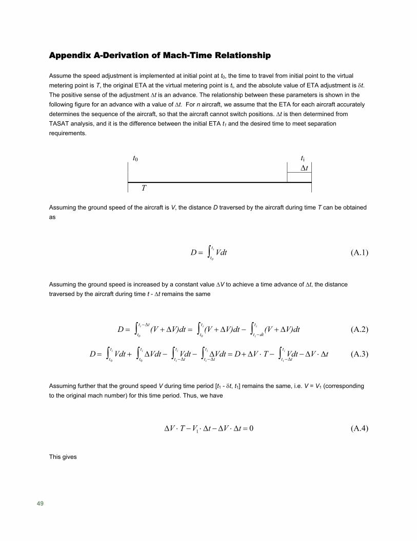
Appendix A-Derivation of Mach-Time Relationship
Assume the speed adjustment is implemented at initial point at t0, the time to travel from initial point to the virtual metering point is T, the original ETA at the virtual metering point is ti, and the absolute value of ETA adjustment is δt. The positive sense of the adjustment Δt is an advance. The relationship between these parameters is shown in the following figure for an advance with a value of Δt. For n aircraft, we assume that the ETA for each aircraft accurately determines the sequence of the aircraft, so that the aircraft cannot switch positions. Δt is then determined from TASAT analysis, and it is the difference between the initial ETA t1 and the desired time to meet separation requirements.
t0 ti
Δt T
Assuming the ground speed of the aircraft is V, the distance D traversed by the aircraft during time T can be obtained as
D = Vdt
t0
ti∫ (A.1)
Assuming the ground speed is increased by a constant value ΔV to achieve a time advance of Δt, the distance traversed by the aircraft during time t - Δt remains the same
D = (V + ΔV)dt
t0
ti −Δt∫ = (V + ΔV)dtt0
ti∫ − (V + ΔV)dtti −dt
ti∫ (A.2)
D = Vdtt0
∫ + ΔVdtt0
∫ − Vdtti −Δt
ti ti ti∫ − ΔVdtti −Δt
ti∫ = D + ΔV ⋅ T − Vdtti −Δt
ti∫ − ΔV ⋅ Δt (A.3)
Assuming further that the ground speed V during time period [t1 - δt, t1] remains the same, i.e. V = V1 (corresponding to the original mach number) for this time period. Thus, we have
ΔV ⋅ T −V1 ⋅ Δt − ΔV ⋅ Δt = 0 (A.4)
This gives
49
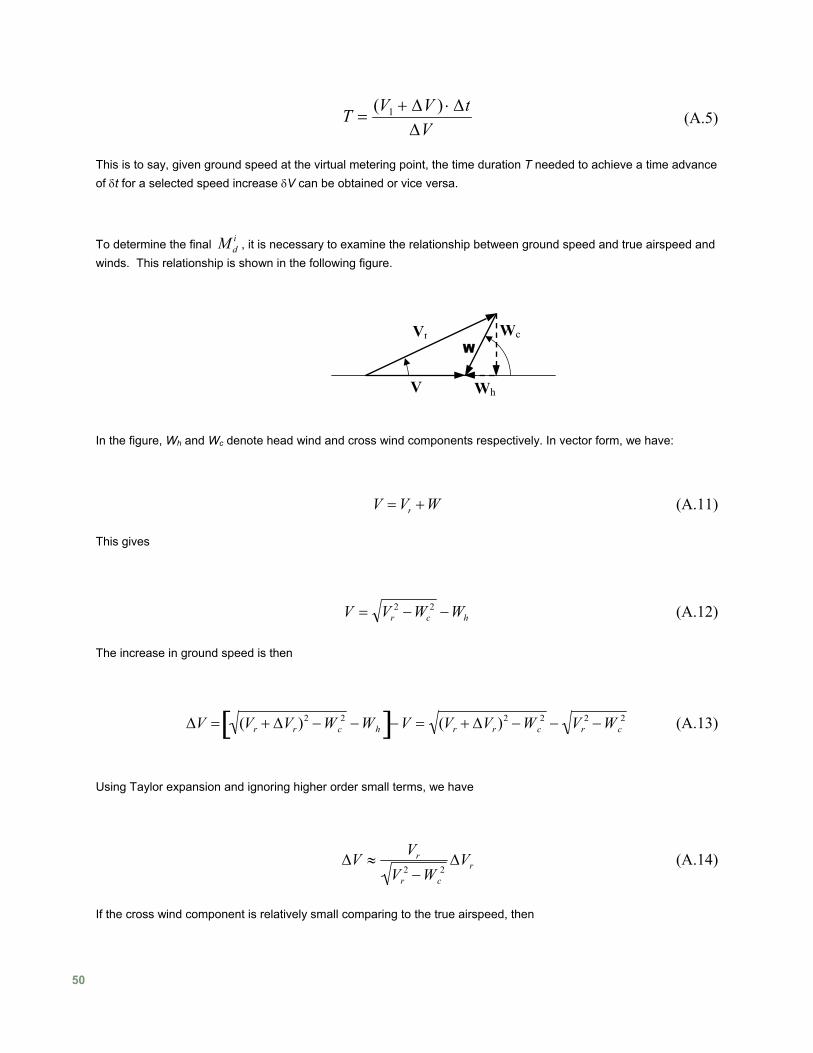
T =(V1 + ΔV ) ⋅ Δt
ΔV (A.5)
This is to say, given ground speed at the virtual metering point, the time duration T needed to achieve a time advance of δt for a selected speed increase δV can be obtained or vice versa.
To determine the final , it is necessary to examine the relationship between ground speed and true airspeed and winds. This relationship is shown in the following figure.
idM
In the figure, Wh and Wc denote head wind and cross wind components respectively. In vector form, we have:
V = Vr +W (A.11)
This gives
hcr WWVV −−= 22 (A.12)
The increase in ground speed is then
ΔV = (Vr + ΔVr)2 −Wc
2 −Wh[ ]−V = (Vr + ΔVr)2 −Wc
2 − Vr2 −Wc
2 (A.13)
Using Taylor expansion and ignoring higher order small terms, we have
ΔV ≈Vr
Vr2 −Wc
2ΔVr (A.14)
If the cross wind component is relatively small comparing to the true airspeed, then
VrW
V
Wh
Wc
50
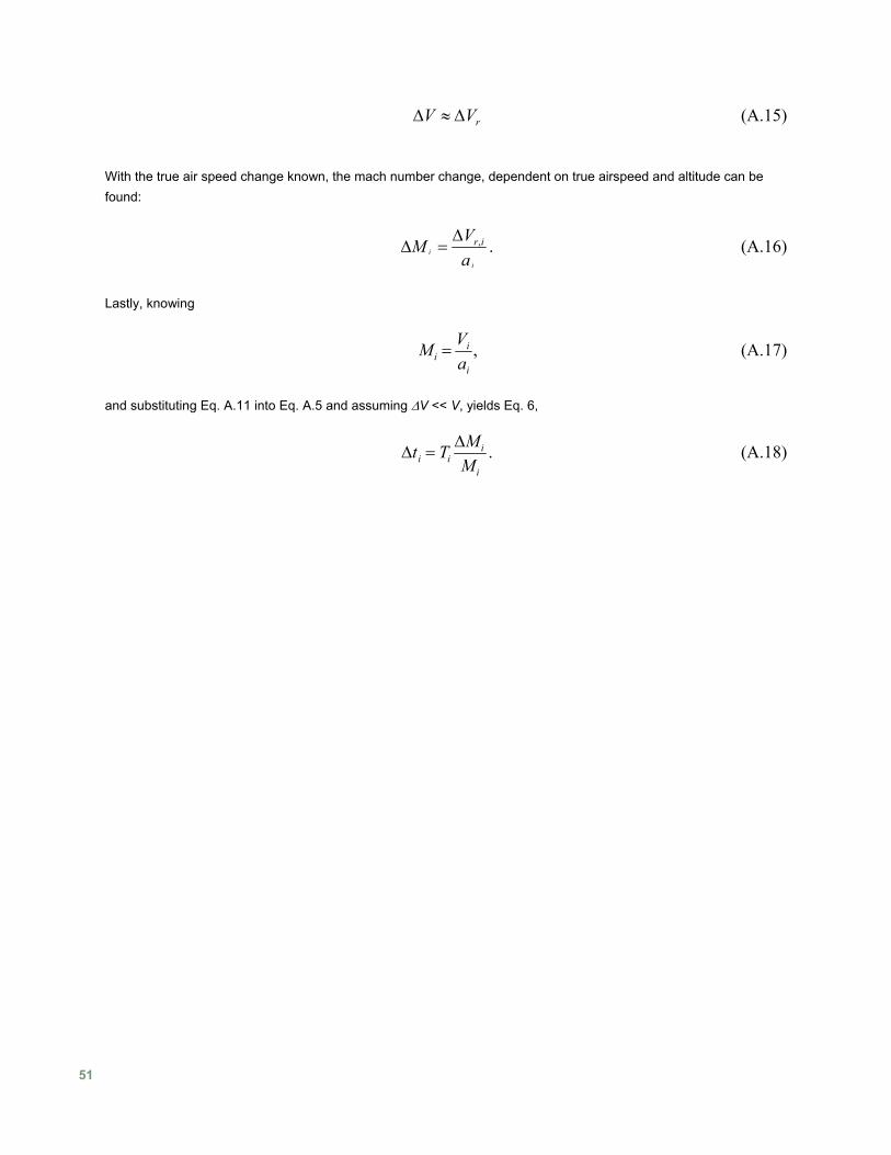
ΔV ≈ ΔVr (A.15)
With the true air speed change known, the mach number change, dependent on true airspeed and altitude can be found:
ΔM i =ΔVr,i
a i
. (A.16)
Lastly, knowing
Mi =Vi
ai
, (A.17)
and substituting Eq. A.11 into Eq. A.5 and assuming ΔV << V, yields Eq. 6,
Δti = TiΔMi
Mi
. (A.18)
51
Appendix B- Nomenclature for En Route Traffic Optimization
ila , : Slope of linear segment of the fuel curve for aircraft i thl
ilb , : Y-intercept of linear segment of the fuel curve for aircraft thl i
iD : Distance aircraft must travel to destination iw
ipD , : Estimated percent increase in distance traveled for aircraft
i
di,1: Distance until the last possible conflict for aircraft i min, jid : Minimum separation between aircraft i and aircraft j
[ iyxi dvdvdv ,= ] : Change in velocity of aircraft between initial condition and final solution. i
D : Initial distance between two aircraft
fuelf : Total cost of objective function
mJ : Infinity Norm weighting cost total fuel burn
sJ : 1-Norm weighting cost for fuel burn
nλλ ,,1 Kr
: SOS2 variables used to estimate speed of an aircraft
[ Tiii yxp = ] : Position of aircraft i
rip : Rotated position of aircraft in relation to angle i ji,Θ
( )jiR ,Θ : Rotation matrix for linear transformation
is : Speed estimate of aircraft i using SOS2 variables
it : Fuel burn for aircraft corresponding to speed changes i
sumt : Sum of total aircraft fuel burn
maxt : Maximum fuel burn over all aircraft
: Estimated fuel costs for aircraft for a heading change i0iθ : Initial heading of aircraft i
ji,Θ : Angle between aircraft i and aircraft and an arbitrary reference line. Used for rotation of variable to
prevent singularities in the solution.
j
( )0,
0,
0 , yixii vvv = : Initial velocity of aircraft i
+iv
r : New velocity command for aircraft i to solve conflict resolution problem
[ Tyixii vvv ,,= ] : Velocity of aircraft i
riv ,+ : Rotated velocity vector of aircraft i in relation to angel ji,Θ
jiv ,~ : Relative velocity between aircraft i and aircraft in rotated frame. j
52
Appendix C- Nomenclature for En Route Spreed Change Optimization for Continuous Descent Arrivals
α
p, q : Sample separation between aircraft p and aircraft q
δi : Binary variable indicating whether this aircraft has a change in Mach
ΔMi : Change in Mach number
Δti : Change in time from initial ETA
ΔT : at grid point λ Δtiη
ki
: Special ordered set 2 (SOS2) indicating which planes corresponding to the fuel burn rate will be used as
approximations
λ1,K,λn : SOS2 variables used to estimate speed of an aircraft λ
kli
: Variable specifying the grid position for ri
μli
: Special ordered set 2 (SOS2) indicating which planes corresponding to Δti will be used as approximations
ai : Speed of sound ai,m : Slope of the mth linear segment of a fuel curve bi,m : y-intercept of the mth linear segment of a fuel curve D : Distance traveled by aircraft
Ý f i : Fuel burn rate for an aircraft at a given Mach number Ý f min : Minimum fuel burn rate
Fk : Fuel burn rate at grid point λ j : Selected number of aircraft able to make a speed change m : Number of lines in the linear interpolation Mbound,I : Maximum or minimum bound on the Mach number change M di
: Final Mach number Mi : Initial Mach number Pfi
: Percentage difference in fuel burn rate change
ri : Variable replacing bilinear term iMtf
id
Δ&
t0,I : Start time of first Mach change tD : Calculated ETA ti : Initial ETA Ti : Total time of Mach speed change Ti,r : Time interval during which the aircraft returns to its original Mach tr : Time at which aircraft returns to its original Mach V : Ground speed of aircraft Vr : Resultant ground speed W : Wind vector WC : Cross wind component of wind vector WH : Head wind component of wind vector
53
54
References
B.T. Baxley, B.E. Barmore, T.S. Abbott, and W.R. Capron. Operational Concept for Flight Crews to Anticipate in Merging and Spacing of Aircraft. 6th AIAA Aviation Technology, Integration and Operations Conference. September 2006. AIAA 2006-7722.
M. van Boven. Development of Noise Abatement Approach Procedures. 10th AIAA/CEAS Aeroacoustics
Conference , Manchester, Great Britain, May 10-12, 2004. AIAA-2004-2810 S.J. Brams and A.D. Taylor. The Win-Win Solution: Guaranteeing Fair Shares to Everybody. W. W. Norton &
Company. 2000. S.J. Brams and A.D. Taylor. Fair Division: From Cake-Cutting to Dispute Resolution. Cambridge: Cambridge
University Press. 1996. J-P. B. Clarke, N.T. Ho, L. Ren, J.A. Brown, K.R. Elmer, K-O. Tong, and J.K. Wat. Continuous Descent
Approach: Design and Flight Test for Louisville International Airport. Journal of Aircraft. Vol. 41, No. September 2004.
R. Deehan. Remarks. Greater Miami Chamber of Commerce Transportation Summit Miami, Florida, November 29, 2006
J. Goss, R. Rajvanshi, and K. Sabarrao, “Aircraft Conflict Detection and Resolution using Mixed Geometric and Collision Cone Approaches,” in Proceedings of the AIAA Guidance, Navigation, and Control Conference and Exhibit, 2004.
J. Hu, M. Prandini, and S. Sastry, “Optimal Coordinated Maneuvers for Three Dimensional Aircraft Conflict
Resolution,” Journal of Guidance, Control and Dynamics, vol. 25, 2002 W. Hylkema and H. Visser, “Aircraft Conflict Resolution Taking into Account Controller Workload using Mixed
Integer Linear Programming,” in Proceedings of the AIAA Guidance, Navigation, and Control Conference and Exhibit, 2003.
H. Idris, T. Hsu, and R. Vivona, “Time Based Conflict Resolution Algorithm and Application to Descent Conflicts,”
in Proceedings of the AIAA Guidance, Navigation, and Control Conference and Exhibit, 2003. J. Kuchar and L. Yang, “A Review of Conflict Detection and Resolution Modeling Methods,” IEEE Transactions on
Intelligent Transportation Systems, vol. 1, 2000. Y. Lebbah, C. Michel, and M. Rueher. “A Rigorous Global Filtering Algorithm for Quadratic Constraints.”
Constraints, 2005. Vol. 10, p. 47-65. A. Nuic, “Aircraft Performance Summary Tables for the Base of Aircraft Data,” EUROCONTROL, Tech. Rep.,
2004. L. Pallottino, E. M. Feron, and A. Bicchi, “Conflict Resolution Problems for Air Traffic Management Systems
Solved With Mixed Integer Programming,” IEEE Transactions on Intelligent Transportation Systems, vol. 3, Mar. 2002.
T. Prevot, .L. Lee, T. Callantine, and N. Smith. “Trajectory-Oriented Time-Based Arrival Operations: Results and
Recommendations.” 4th USA/Europe Air Traffic Management Research and Development Seminar, Air-Ground Cooperation Track, Budapest, Hungary, 2003.
R. Vivona, D. Karr, and D. Roscoe, “Pattern Based Genetic Algorithm for Airborne Conflict Resolution,” in
Proceedings of the AIAA Guidance, Navigation, and Control Conference and Exhibit, 2006. J. Wat, J. Follet, R. Mead, J. Brown R. Kok, F. Dijkstra, and J. Vermeij. In Service Demonstration of Advanced
Arrival Techniques at Schiphol Airport. 6th AIAA Aviation Technology, Integration and Operations Conference (ATIO), Wichita, Kansas, Sep. 25-27, 2006. AIAA-2006-7753.

L.A. Weitz, J.E. Hurtado, and F. J. L. Bussink. Increasing Runway Capacity for Continuous Descent Approaches
Through Airborne Precision Spacing. AIAA Guidance, Navigation, and Control Conference and Exhibit 15-18 August 2005, San Francisco, California. AIAA 2005-6142.
K.D. Wichman, G. Carlsson, and L.G. V. Lindberg. Flight trials: “runway-to-runway” required time of arrival
evaluations for time-based ATM environment. Digital Avionics Systems, 2001. DASC. The 20th Conference. October 2001. Vol. 2, 7F6/1-7F6/13.
.
55