EMULATION OF ANALOG CONTROLLERSmocha-java.uccs.edu/ECE5540/ECE5540-CH02.pdf · ECE4540/5540, EMULATION OF ANALOG CONTROLLERS 2–9 Performance not great, so tried again with T = 0.1ms.Much

ECE4540/5540: Digital Control Systems 2–1

EMULATION OF ANALOG CONTROLLERS

2.1: Control design via time-domain emulation

■ There are two main approaches to digital controller design:

1. Emulation—we look at this now (two methods).

2. Direct digital design—subject of the rest of the course.

■ Emulation is when a digital computer approximates an analog

controller design.

■ Analog:

D(s) G(s) y(t)r (t)u(t)e(t)

■ Digital:

zohD2AA2D

]

D(z) G(s)Q

w(t)

v(t)

y(t)r (t)u(t)u[k]e(t) e[k]

■ Analog controller computes u(t) from e(t) using differential equations.

■ Digital controller computes u(kT ) from e(kT ) using difference

equations.

■ To interface the computer controller to the “real world” we need an

analog-to-digital converter (to measure analog signals) and

digital-to-analog converter (to output signals).

Lecture notes prepared by Dr. Gregory L. Plett. Copyright © 2017, 2009, 2004, 2002, 2001, 1999, Gregory L. Plett

ECE4540/5540, EMULATION OF ANALOG CONTROLLERS 2–2

■ Sampling and outputting usually done synchronously, at a constant

rate. If sampling period = T, frequency = 1/T .

■ The signals inside the computer (the sampled signals) are noted as

y(kT ), or simply y [k]. y [k] is a discrete-time signal, where y(t) is a

continuous-time signal.

(system

y(t) y(kT )

■ Discrete-time signals are usually converted to continuous-time

signals using a zero-order hold:

e.g., to convert u [k] to u(t).

■ We will spend more time on these topics as the course progresses.

Only a conceptual understanding is needed now.

“Digitization”

■ Continuous-time controllers are designed with Laplace-transform

techniques. The resulting controller is a function of “s”.

y(t) =dx(t)

dtx(t) s

■ So, “s” is a derivative operator. There are several ways of

approximating this in discrete time. We look at one now called the

“forward rectangular” rule.

x(t)!= lim

δt→0

δx(t)

δt= lim

δt→0

x(t + δt) − x(t)

δt.



■ If T is small,

x(kT ) ≈x((k + 1)T ) − x(kT )

Ti.e., x[k] ≈

x[k + 1] − x[k]T

.

■ To use this approximation, we set T = tk+1 − tk = sampling interval.

■ We “digitize” a controller D(s) by

1. Noting that controller output is related to controller input via

U (s) = D(s)E(s).

2. Performing term-by-term inverse Laplace transform to get a

differential equation relationship between u(t) and e(t)n∑

k=0

ak

dku(t)

dt k=

m∑

k=0

bk

dke(t)

dt k.

3. Replace derivatives with differences.

EXAMPLE:

■ Consider D(s) =U (s)

E(s)= k0

s + a

s + b. . . a lead or lag controller.

1. (s + b)U (s) = k0(s + a)E(s).

2. u(t) + bu(t) = k0e(t) + ak0e(t).

3. Use “forward rectangular rule” to digitizeu[k + 1] − u[k]

T+ bu[k] = k0

(

e[k + 1] − e[k]T

+ ae[k])

u[k + 1] = u[k] +

T

[

−bu[k] + k0

(

e[k + 1] − e[k]T

+ ae[k])]

u[k + 1] = (1 − bT )u[k] + k0(aT − 1)e[k] + k0e[k + 1].

■ Note that we often re-index the difference equation to be in more

familiar terms of “k” instead of “k + 1”

u[k] = (1 − bT )u[k − 1] + k0(aT − 1)e[k − 1] + k0e[k].



■ Present output of digital controller u[k] depends on previous output

u[k − 1] as well as the previous and current errors e[k − 1] and e[k].

Real-Time Controller Implementation

x = 0. (initialization of “past” values for first loop through)

Define constants:

α1 = 1 − bT .

α2 = k0(aT − 1).

READ A/D to obtain y[k] and r [k].

e[k] = r [k] − y[k].

u[k] = x + k0e[k].

OUTPUT u[k] to D/A and ZOH.

Now compute x for the next loop through:

x = α1u[k] + α2e[k].

Go back to “READ” when T seconds have elapsed since last READ.

■ Code is optimized to minimize latency between A2D read and D2A

write.

R = read. W = write.C = compute. I = idle.

R RR CCC WWW III

T

■ Rule of thumb: Sampling frequency must be ≈ 30 times the

bandwidth of the analog system for comparable performance.

EXAMPLE: This one with numbers:

■ Let D(s) = 70(s + 2)

(s + 10), G(s) =

1

s(s + 1).

■ Choose to try a sample rate of 20 Hz and also try 40 Hz.



(Note, BW of analog system is ≈ 1 Hz or so).

➠ Use formula from before to digitize D(s).

■ 20 Hz: u[k + 1] = 0.5u[k] + 70e[k + 1] − 63e[k].

■ 40 Hz: u[k + 1] = 0.75u[k] + 70e[k + 1] − 66.5e[k].

0 0.2 0.4 0.6 0.8 10

0.5

1

1.5

analogdigital

]1

Time (sec)

Pla

nt

outp

ut

Sampled at 20Hz

0 0.2 0.4 0.6 0.8 10

0.5

1

1.5

analogdigital

Time (sec)

Pla

ntoutp

ut

Sampled at 40Hz

■ IMPORTANT NOTE: The closed loop system with digital controller

has poorer damping than the original analog system. This will always

be true when emulating an analog controller. We see why next . . .



2.2: The importance of the D2A “hold” operation

u(t)

avg. u(t)

u(kT )u

■ Even if u(kT ) is a perfect re-creation of the output of the analog

controller at t = kT , the “hold” in the D2A causes an “effective delay.”

■ The delay is approximately equal to half of the sampling period: T/2.

■ Recall from frequency-response analysis and design, the magnitude

of a delayed response stays the same, but the phase changes:

!phase = −ωT

2.

■ For the previous example, sampling now at 10 Hz, we have:

10−1

100

101

102

10−1

100

101

10−1

100

101

102

−180

−160

−140

−120

−100

Frequency (rad/sec)

Magnitu

de

Phase

(Deg)

■ The PM has changed from ≈ 50◦ to ≈ 30◦.

■ ζ ≈PM

100. . . ζ changed from 0.5 to 0.3 . . . much less damping.



■ Mp from about 20% to about

30% . . .

■ Faster sampling. . . smaller T . . .

smaller delay. . . smaller change

in response.0 0.2 0.4 0.6 0.8 1

0

0.5

1

1.5

Time (sec)

Pla

nt

outp

ut

Root-locus view of the delay

■ Recall that we can model a delay using a Padé approximation.

T

2delay −→ e−sT/2 ≈

1 − sT/4

1 + sT/4.

■ Poles and zeros reflected about the jω-axis.

−4

T

4

T

I(s)

R(s)As T → 0, delay dynamics → ∞.

■ Impact of delay: Suppose D(s)G(s) =1

s + a.

Nominal

−a

I(s)

R(s)

With

delay

➠ −4

T

4

T

−a

I(s)

R(s)



■ Does the delayed locus make sense?

1 − sT/4

1 + sT/4= −

(sT/4 − 1)

(sT/4 + 1).

■ Gain is negative! We need to draw a 0◦ root locus, not the 180◦ locus

we are more familiar with.

■ Conclusion: Delay destabilizes the system.

PID Control via Emulation

P: u(t) = K e(t)

I: u(t) =∫ t

0

K

TI

e(τ ) dτ

D: u(t) = K TDe(t)

⎫

⎪⎪⎪⎬

⎪⎪⎪⎭

PID: u(t) = K

[

e(t) +1

TI

∫ t

0

e(τ ) dτ + TDe(t)

]

or, u(t) = K

[

e(t) +1

TI

e(t) + TDe(t)

]

.

■ Convert to discrete-time (use rule twice for e(t)).

u[k] = u[k−1]+K

[(

1 +T

TI

+TD

T

)

e[k] −(

1 +2TD

T

)

e[k − 1] +TD

Te[k − 2]

]

.

EXAMPLE:

G(s) =360000

(s + 60)(s + 600)K = 5, TD = 0.0008, TI = 0.003.

■ Bode plot of cts-time OL system D(s)G(s) with the above PID D(s)

shows that BW ≈ 1800 rad s−1 ≈ 320 Hz.

10 × BW ➠ T = 0.3 ms.

■ From above,

u[k] = u[k − 1] + 5

[

3.7667e[k] − 6.333e[k − 1] + 2.6667e[k − 2]]

.



■ Performance not great, so tried

again with T = 0.1 ms. Much

better.

■ Note, however, that the error is

mostly due to the rise time

being too fast, and the damping

too low.0 2 4 6 8 10

0

0.2

0.4

0.6

0.8

1

1.2

1.4

continuousdigital: T=0.3msecdigital: T=0.1msec

Time (msec)

Speed

(rads/

sec)

■ FIDDLE with parameters ➠

increase K to slow the system

down; Increase TD to increase

damping. ➠ New K = 3.2, new

TD = 0.3 ms.0 2 4 6 8 10

0

0.5

1

1.5

continuousdigital: T=0.3msec

Time (msec)

Speed

(rads/

sec)

KEY POINT: We can emulate a desired analog response using the

forward-rectangular rule, but the delay added to the system due to the

D2A hold circuit will decrease damping. This could even destabilize

the system!!! This delay can be minimized by sampling at a high rate.

(EXPENSIVE). Or, we can change the digital controller parameters,

as in the last example, to achieve the desired system performance

BUT NOT BY emulating the specific analog controller D(s).

■ How do we design the digital controller if we cannot use D(s) as a

prototype? Need Laplace-like tools for discrete-time.

THE z-TRANSFORM!



2.3: Definition of the z-transform

■ In ECE4510/5510, we saw that the Laplace transform is a very

powerful tool for analysis and design of analog control systems.

■ We are now looking at discrete-time (digital) control systems, and we

need a similar tool. Enter the z-transform. . .

DEFINITION: The (one-sided or unilateral) z-transform is defined as

X (z) = x(0) + x(T )z−1 + x(2T )z−2 + x(3T )z−3 + · · ·

=∞∑

k=0

x(kT )z−k

(

or, X (z) =∞∑

k=0

x[k]z−k.

)

■ Like the Laplace-transform variable “s,” the z-transform variable “z” is

a complex number.

■ Like the Laplace-transform, convergence of the transform is an

important consideration.

• For the above definition of the z-transform, convergence is always

of the form

X (z) = something, |z| > ρ,

where ρ is a disc on the z-plane.



EXAMPLE: Define the digital impulse (unit pulse) function to be

δ[k] =

{

1, k = 0;0, otherwise.

−4 −2 0 2 4 6 8■ Note: This is very different from an analog impulse (e.g., δ[0] is

defined), but plays a similar role.

so, let x[k] = δ[k]

X (z) =∞∑

k=0

x[k]z−k

= x[0]z0 + x[1]z−1 + x[2]z−2 + · · ·

= x[0] = 1.

■ Since this sum converges to 1 regardless of the value of z,

ROC = {|z| > 0}.

EXAMPLE: Consider a delayed impulse:

−4 −2 0 2 4 6 8

x[k] = δ[k − kd]

X (z) =∞∑

k=0

x[k]z−k

= x[0] + x[1]z−1 + · · · + x[kd]z−kd + · · ·

= x[kd]z−kd = z−kd .

■ Again, ROC = {|z| > 0}.



EXAMPLE: Let x[k] be the discrete unit-step function.

x[k] = 1[k] =

{

1, k ≥ 0;0, otherwise.

1(z) =∞∑

k=0

1[k]z−k

=∞∑

k=0

z−k = 1 + z−1 + z−2 + · · ·

−4−2 0 2 4 6 8

■ Multiply both sides of this equation by (z − 1).

(z − 1)1(z) = (z + 1 + z−1 + z−2 + · · · ) − (1 + z−1 + z−2 + · · · )

= z − z−∞ (in the limit)

= z if |z| > 1.

so 1(z) =z

z − 1, ROC = {|z| > 1}.

EXAMPLE: Let x[k] = ak1[k] where a is a complex number.

X (z) =∞∑

k=0

akz−k

= 1 + az−1 + a2z−2 + · · · −4−2 0 2 4 6 8

■ Multiply both sides of this equation by (z − a).

(z − a)X (z) = (z + a + a2z−1 + · · · ) − (a + a2z−1 + a3z−2 + · · · )

= z − a∞z−∞ (in the limit)

= z if |z| > |a|

so X (z) =z

z − a, ROC = {|z| > |a|}.



2.4: Delay properties of the z-transform

Linearity:

■ The standard linearity rule:

• If x[k] ↔ X (z) and v[k] ↔ V (z),

• Then ax[k] + bv[k] ↔ aX (z) + bV (z). (prove for yourself)

EXAMPLE: Let y[k] = 1[k] + ak1[k].

■ Then,

Y (z) =z

z − 1+

z

z − a=

2z2 − (1 + a)z

(z − 1)(z − a).

Right shift in time (delay); Theorem 1:

■ Suppose x[k] ↔ X (z), and q is a positive integer.

y[k] = x[k − q]1[k − q]

Y (z) =∞∑

k=0

x[k − q]1[k − q]z−k let k = k − q

=∞∑

k=−q

x[k]1[k]z−(k+q)

= z−q

∞∑

k=0

x[k]z−k

= z−q X (z).

■ So, a delay of q samples multiplies the z-transform by z−q.

EXAMPLE:

p[k] =

{

1, k = 0, 1, . . . N − 1;0, otherwise.



■ Note that p[k] = 1[k] − 1[k − N ].

■ By linearity and by the right-shift theorem,

P(z) = 1(z) − z−N 1(z)

=z

z − 1− z−N z

z − 1

=zN − 1

zN−1(z − 1).

Right shift in time (delay); Theorem 2:

■ The first delay theorem states: x[k − q]1[k − q] ⇐⇒ z−q X (z).

■ The second delay theorem states: x[k − q] ⇐⇒ . . .

■ The first version is generally used on causal signals. The second

version is generally used on non-causal signals or when analyzing

effect of systems that may have initial conditions.

x[k − 1] ⇐⇒ z−1X (z) + x[−1]

x[k − 2] ⇐⇒ z−2X (z) + x[−2] + z−1x[−1]

...

x[k − q] ⇐⇒ z−q X (z) + x[−q] + z−1x[−q + 1] + · · · + z−q+1x[−1].

■ Proof for the first case:

x[k − 1] ⇐⇒∞∑

k=0

x[k − 1]z−k let k = k − 1

=∞∑

k=−1

x[k]z−(k+1)



= x[−1] +∞∑

k=0

x[k]z−(k+1)

= x[−1] + z−1X (z). Proof of other cases by induction.

EXAMPLE: z-transform of LCCDE.

■ Many discrete-time systems are described by Linear Constant

Coefficient Difference Equations (LCCDEs). These are of the formn∑

i=0

ai y[k − i] =m∑

i=0

bi x[k − i],

where n > m.

■ We can find the transfer function of this system by taking the

z-transform of both sides of this equation.

■ System transfer functions always assume zero initial conditions, so

we can use Delay Theorem 1.n∑

i=0

ai z−iY (z) =

m∑

i=0

bi z−i X (z),

H(z) =Y (z)

X (z)

=∑m

i=0 bi z−i

∑ni=0 ai z−i

.

■ We can multiply numerator and denominator by zn to get it in terms of

positive powers of z.

EXAMPLE: Find the output of a system described by difference equation

y[k] + 0.5y[k − 1] = x[k],

where x[k] = 1[k] and y[−1] = 6.



■ There are initial conditions, so we use Delay Theorem 2,

Y (z) + 0.5[

z−1Y (z) + y[−1]]

= X (z)

Y (z)[1 + 0.5z−1] =z

z − 1− 3

Y (z) =z − 3(z − 1)

(z − 1)(1 + 0.5z−1)

=3z − 2z2

(z − 1)(z + 0.5)

=−(8/3)z

z + 0.5+

(2/3)z

z − 1

y[k] =2

3· 1[k] −

8

3(−0.5)k1[k].



2.5: Time multiplication and the z-transform

Multiplication by k and k2.

■ What happens when we multiply a time sequence x[k] by k or k2?

■ Recall:

X (z) =∞∑

k=0

x[k]z−k.

■ Then,

d

dzX (z) =

∞∑

k=0

−kx[k]z−k−1

= −z−1

∞∑

k=0

kx[k]z−k

︸︷︷︸

Y (z)

.

■ Thus,

kx[k] ⇐⇒ −zd

dzX (z).

■ Also

k2x[k] ⇐⇒ zd

dzX (z) + z2 d2

dz2X (z).

EXAMPLE: Recall that ak1[k] ↔z

z − a.

d

dz

(

z

z − a

)

=[

−z

(z − a)2+

1

z − a

]

=−a

(z − a)2

so, kak1[k] ↔az

(z − a)2

and, k1[k] ↔z

(z − 1)2. (ramp)



Multiplication by ak:

■ Multiply a time sequence x[k] by ak (a complex).

akx[k] ↔∞∑

k=0

akx[k]z−k

=∞∑

k=0

x[k]( z

a

)−k

= X (z/a).

Multiplication by cos[ωk] and sin[ωk].

■ Multiply a time sequence x[k] by cos[ωk] or sin[ωk].

■ Recall from Euler’s theorem

cos[ωk] =e jωk + e− jωk

2and sin[ωk] =

e jωk − e− jωk

2 j.

■ So,

cos[ωk]x[k] ⇐⇒1

2X(

e− jωz)

+1

2X(

e jωz)

sin[ωk]x[k] ⇐⇒1

2 jX(

e− jωz)

−1

2 jX(

e jωz)

.

EXAMPLE: Find the z-transform of x[k] = cos[ωk]1[k].

■ Recall that 1[k] ⇐⇒z

z − 1.

X (z) =1

2

(

e jωz

e jωz − 1+

e− jωz

e− jωz − 1

)

=1

2

(

e jωz(e− jωz − 1) + e− jωz(e jωz − 1)

(e jωz − 1)(e− jωz − 1)

)



=1

2

(

z2 − e jωz + z2 − e− jωz

z2 − (e jω + e− jω)z + 1

)

cos[ωk]1[k] ⇐⇒z2 − cos[ω]z

z2 − (2 cos[ω])z + 1.

■ Also,

sin[ωk]1[k] ⇐⇒z sin[ω]

z2 − (2 cos[ω])z + 1.



2.6: Convolution, initial/final value and the z-transform

Convolution

■ Discrete-time convolution is analogous to continuous-time

convolution:

(x ∗ v)[k] =k∑

i=0

x[i]v[k − i] k ≥ 0

or, =k∑

i=0

v[i]x[k − i]. k ≥ 0.

■ Assuming that x[k] and v[k] are zero for negative k,

(x ∗ v)[k] =∞∑

i=0

x[i]v[k − i] k ≥ 0

⇐⇒∞∑

k=0

[∞∑

i=0

x[i]v[k − i]

]

z−k

=∞∑

i=0

∞∑

k=0

x[i]v[k − i]z−k

=∞∑

i=0

x[i]

[∞∑

k=0

v[k − i]z−k

]

k = k − i

=∞∑

i=0

x[i]

⎡

⎣

∞∑

k=−i

v[k]z−(k+i)

⎤

⎦

=∞∑

i=0

x[i]

⎡

⎣

∞∑

k=0

v[k]z−k

⎤

⎦ z−i

= X (z)V (z).



Initial-value theorem

■ If x[k] ⇐⇒ X (z), x[0] = limz→∞

X (z).

■ Proof:

X (z) =∞∑

k=0

x[k]z−k

= x[0] + x[1]z−1 + x[2]z−2 + · · ·

as z → ∞, = x[0] + x[1] · 0 + x[2] · 0 + · · ·

= x[0].

■ Also,

x[1] = limz→∞

(zX (z) − zx[0])

x[2] = limz→∞

(

z2 X (z) − z2x[0] − zx[1])

...

Final value theorem

■ Proof not too enlightening:

limk→∞

x[k] = limz→1

(z − 1)X (z)

assuming the limit on the left exists! Conditions for existence: All

poles of X (z) must be inside unit circle |pi | < 1 ∀ i , except possibly a

single pole on the unit circle at z = 1. The residue of the pole at z = 1

is the final value and is found from above.

EXAMPLE:

■ Suppose X (z) =3z2 − 2z + 4

z3 − 2z2 + 1.5z − 0.5.



■ Factoring the denominator:

X (z) =3z2 − 2z + 4

(z − 1)(z2 − z + 0.5)

xss =3z2 − 2z + 4

(z2 − z + 0.5)

∣∣∣∣z=1

=5

0.5= 10.



2.7: The inverse z-transform

1.] Power-series method:

■ Suppose X (z) =z2 − 1

z3 + 2z + 4,

■ Dividing:

z−1 +0z−2 −3z−3 −4z−4 · · ·z3 + 2z + 4

)

z2 −1

z2 +2 +4z−1

−3 −4z−1

−3 −6z−2 −12z−3

−4z−1 +6z−2 +12z−3

−4z−1 −8z−3 −16z−4

6z−2 +20z−3 +16z−4

...

■ So, X (z) = z−1 − 3z−3 − 4z−4 · · · .

■ and x[0] = 0, x[1] = 1, x[2] = 0, x[3] = −3, x[4] = −4, . . .

2.] Partial-fraction expansion

■ Recall that partial-fraction expansion was used to take

inverse-Laplace transforms of things like:

H(s) =num(s)

den(s),

where the order of num(s) <order of den(s).

■ z-transforms almost always have the same order numerator and

denominator which requires modifying the technique slightly.

■ Let X (z) =N (z)

D(z)and let D(z) have distinct poles.



■ Do partial-fraction expansion onX (z)

z=

N (z)

zD(z).

X (z)

z=

r0

z+

r1

z − p1

+r2

z − p2

+ · · · +rn

z − pn

r0 =[

zX (z)

z

]

z=0

= X (0)

ri =[

(z − pi)X (z)

z

]

z=pi

i = 1, . . . , n.

■ So,

X (z) = r0 +r1z

z − p1

+r2z

z − p2

+ · · · +rnz

z − pn

.

• Transforming: r0 ⇐⇒ r0δ[k].

• Transforming:ri z

z − pi

⇐⇒ ri pki 1[k].

• Note:

r1 pk1 + r1 pk

1 = 2 |r1| |p1|k cos[

k p1 + r1

]

k = 0, 1, . . .

if r1 and p1 complex.

EXAMPLE:

■ Suppose

X (z) =z3 + 1

z3 − z2 − z − 2

=z3 + 1

(z − 2)(

z + 12+ j

√3

2

) (

z + 12− j

√3

2

)

X (z)

z=

r0

z+

r1

z + 12+ j

√3

2

+r1

z + 12− j

√3

2

+r2

z − 2.



■ Find the residues:

r0 = X (0) =−1

2

r1 =

⎡

⎢

⎣

z3 + 1

(z − 2)(

z + 12− j

√3

2

)

1

z

⎤

⎥

⎦

z=−12− j

√3

2

=3

7+ j

√3

21

r2 =[

(z − 2)X (z)

z

]

z=2

=9

14.

■ So,

x[k] = −1

2δ[k]+r1

(

−1

2− j

√3

2

)k

1[k]+r1

(

−1

2+ j

√3

2

)k

1[k]+9

142k1[k].

■ Note: |p1| = 1, p1 = 4π/3. |r1| = 0.436, r1 = 10.89◦.

■ So,

x[k] = −1

2δ[k] + 0.873 cos

(

4π

3k + 10.89◦

)

1[k] +9

14(2)k 1[k].

Repeated poles:

■ There is a special rule for repeated poles, just as with

Laplace-transform partial-fraction expansion.

■ Suppose p1 is repeated “n” times.

X (z)

z=

r0

z+

r1,1

z − p1

+r1,2

(z − p1)2+ · · · +

r1,n

(z − p1)n+ other poles

■ Then, the residues are calculated as

r1,n =[

(z − p1)n X (z)

z

]

z=p1

r1,n−1 =1

1!

[

d

dz

(

(z − p1)n X (z)

z

)]

z=p1



r1,n−2 =1

2!

[

d2

dz2

(

(z − p1)n X (z)

z

)]

z=p1

...

r1,1 =1

(n − 1)!

[

dn−1

dzn−1

(

(z − p1)n X (z)

z

)]

z=p1

.

■ MATLAB’s residue command automates partial-fraction expansion:

num=[ ] % coefficients of numerator.

den=[] % coefficients of denominator.

[r,p,k]=residue(num,[den 0]) % don't forget '1/z'!

■ Or, there is a somewhat easier way:

num=[ ] % coefficients of numerator.

den=[] % coefficients of denominator.

[r,p,k]=residuez(num,den)

■ Be sure to type help residue or help residuez if there are

repeated roots to understand the format of the results that MATLAB

returns.

3.] Inversion formula:

■ A third way to invert a z-transform is to use the relationship:

x[k] =1

2π j

∮

)

X (z)zk−1 dz

where this is a counter-clockwise contour integral over the path ) in

the z-plane. ) must be in the region of convergence.

■ This looks terrible, but the theorem of residues makes it simpler. It

reduces to:

x[k] =

⎡

⎢

⎣

∑

all poles of X (z)zk−1

[residues of X (z)zk−1]

⎤

⎥

⎦ 1[k].



■ For a simple pole of X (z)zk−1 at a, the residue is:

[residue]z=a = (z − a)X (z)zk−1∣∣z=a

.

■ For a repeated pole of X (z)zk−1 at a, repeated m times,

[residue]z=a =1

(m − 1)!dm−1

dzm−1

[

(z − a)m X (z)zk−1]

z=a.

EXAMPLE:

X (z) =z

(z − 1)(z − 2).

■ So,

x[k] =[

zk

z − 2

∣∣∣∣z=1

+zk

z − 1

∣∣∣∣z=2

]

1[k]

=[

−1 + 2k]

1[k].

EXAMPLE:

X (z) =z

(z − 1)2.

x[k] =[

1

(2 − 1)!d2−1

dz2−1

[

(z − 1)2 z

(z − 1)2zk−1

]

z=1

]

1[k]

=[

d

dzzk

∣∣∣∣z=1

]

1[k]

= kzk−1∣∣z=1

1[k]

= k1[k].


ECE4540/5540, EMULATION OF ANALOG CONTROLLERS 2–28L

apla

cetr

ansf

orm

Tim

efu

nct

ion

z-T

ran

sfo

rmM

od

ified

z-tr

ansf

orm

E(s

)e(

t)E

(z)

E(z

,m)

1 s1(t

)z

z−1

1z−

1

1 s2t1

(t)

Tz

(z−

1)2

mT

z−1

+T

(z−

1)2

1 s3t2 2

1(t

)T

2z(

z+1)

2(z

−1)3

T2 2

[

m2

z−1

+2m

+1

(z−

1)2

+2

(z−

1)3

]

(k−

1)!

sktk

−11(t

)li

ma→

0(−

1)k

−1

∂k−

1

∂a

k−

1

[

zz−

e−a

T

]

lim

a→

0(−

1)k

−1

∂k−

1

∂a

k−

1

[

e−a

mT

z−e−

aT

]

1s+

ae−

at 1

(t)

zz−

e−a

Te−

am

T

z−e−

aT

1(s

+a)2

te−

at 1

(t)

Tze

−a

T

(z−

e−a

T)2

Te−

am

T[e

−a

T+

m(z

−e−

aT)]

(z−

e−a

T)2

(k−

1)!

(s+

a)k

tke−

at 1

(t)

(−1)k

∂k

∂a

k

[

zz−

e−a

T

]

(−1)k

∂k

∂a

k

[

e−a

mT

z−e−

aT

]

as(

s+a)

1−

e−a

tz(

1−

e−a

T)

(z−

1)(

z−e−

aT)

1z−

1−

e−a

mT

z−e−

aT

as2

(s+

a)

t−

1−

e−a

T

az[

(aT

−1+

e−a

T)z

+(a

−e−

aT−

aT

e−a

T)]

a(z

−1)2

(z−

e−a

T)

T(z

−1)2

+a

mT

−1

a(z

−1)

+e−

am

T

a(z

−e−

aT)

a2

s(s+

a)2

1−

(1+

at)

e−a

tz

z−1

−z

z−e−

aT

−a

Te−

aT

z(z

−e−

aT)2

1z−

1−[

1+

am

Tz−

e−a

T+

aT

e−a

T

(z−

e−a

T)2

]

e−a

mT

b−

a(s

+a)(

s+b)

e−a

T−

e−b

T(e

−a

T−

e−b

T)z

(z−

e−a

T)(

z−e−

bT)

e−a

mT

z−e−

aT

−e−

bm

T

z−e−

bT

as2

+a

2si

n(a

t)z

sin(a

T)

z2−

2z

cos(

aT

)+1

zsi

n(a

mT

)+si

n((

1−

m)a

T)

z2−

2z

cos(

aT

)+1

ss2

+a

2co

s(a

t)z(

z−co

s(a

T))

z2−

2z

cos(

aT

)+1

zco

s(a

mT

)−co

s((1

−m

)aT

)z2

−2

zco

s(a

T)+

1

b(s

+a)2

+b

2e−

at

sin(b

t)ze

−a

Tsi

n(b

T)

z2−

2ze

−a

Tco

s(b

T)+

e−2a

Te−

am

T[z

sin(b

mT

)+e−

aT

sin((

1−

m)b

T)]

z2−

2ze

−a

Tco

s(b

T)+

e−2a

T

s+a

(s+

a)2

+b

2e−

atco

s(b

t)z2

−ze

−a

Tco

s(b

T)

z2−

2ze

−a

Tco

s(b

T)+

e−2a

Te−

am

T[z

cos(

bm

T)+

e−a

Tsi

n((

1−

m)b

T)]

z2−

2ze

−a

Tco

s(b

T)+

e−2a

T

a2+

b2

s[(s

+a)2

+b

2]

1−

e−a

t(

cos(

bt)

+a b

sin(b

t))

z(A

z+B

)(z

−1)(

z2−

2ze

−a

Tco

s(b

T)+

e−2a

T)

1z−

1−

...

A=

1−

e−a

T(

cos(

bT

)+

a bsi

n(b

T))

e−a

mT[z

cos(

bm

T)+

e−a

Tsi

n((

1−

m)b

T)]

z2−

2ze

−a

Tco

s(b

T)+

e−2a

T+

...

B=

e−2a

T+

e−a

T(

a bsi

n(b

T)−

cos(

bT

))a b(e

−a

mT[z

sin(b

mT

)−e−

aT

sin((

1−

m)b

T)])

z2−

2ze

−a

Tco

s(b

T)+

e−2a

T

1s(

s+a)(

s+b)

1 ab

+e−

at

a(a

−b)+

e−b

t

b(b

−a)

(Az+

B)z

(z−

e−a

T)(

z−e−

bT)(

z−1)

A=

b(1

−e−

aT)−

a(1

−e−

bT)

ab(b

−a)

B=

ae−

aT(1

−e−

bT)−

be−

bT(1

−e−

aT)

ab(b

−a)



2.8: Time responses versus pole locations

■ We found that the Laplace-transform pole locations determined time

response. The same is true of the z-transform.

Unit step:

■ x[k] = 1[k].

■ X (z) =z

z − 1, |z| > 1.

−4−2 0 2 4 6 8

Exponential (geometric):

■ x[k] = ak1[k], |a| < 1.

■ X (z) =z

z − a, |z| > |a|.

−4−2 0 2 4 6 8

General cosinusoid:

■ x[k] = ak cos[ωk]1[k], |a| < 1.

■ X (z) =z(z − a cos ω)

z2 − 2a(cos ω)z + a2, |z| > |a|. −4−2 0 2 4 6 8

■ The radius to the two poles is a.

■ The angle to the poles is ω.

■ The zero (not at the origin) has the same real part as the two poles.

■ Note: If ω = 0, X (z) =z

z − a. . . exponential!

■ If ω = 0, a = 1, X (z) =z

z − 1. . . step!



■ Radius of pole locations is the exponential factor, and determines

settling time.

1. |a| > 1, Growing signal which will not decay.

2. |a| = 1, Signal with constant amplitude; either step or cosine.

3. |a| < 1, Decaying signal. Small a = fast decay (see below).

a ≈ duration N

0.9 43

0.8 21

0.6 9

0.4 5

4. |a| = 0, Finite-duration response. e.g., δ[k − N ] ⇐⇒ z−N .

■ Angle of pole locations, ω, determines number of samples per

oscillation.

• That is, require cos[ωk] = cos[ω(k + N )].

N =2π

ω

∣∣∣∣rad

=360

ω

∣∣∣∣deg

samples/cycle.

N = 2

N = 3

N = 4 N = 5

N = 8N = 10

N = 20

■ Solid lines are constant damping ratio ζ .

■ Dashed lines are constant natural frequency ωn.



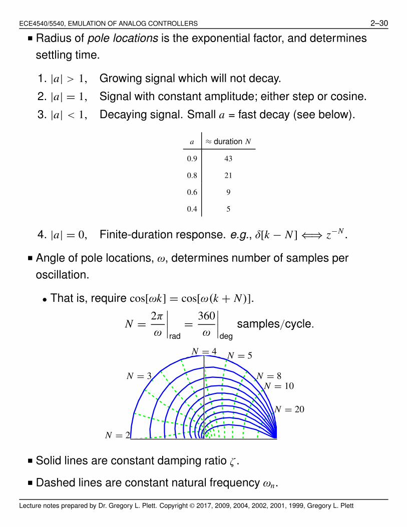
Discrete Impulse Responses versus Pole Locations

R(z)

I(z)

Correspondence with continuous signals

■ Let x(t) = e−at cos(bt)1(t).

■ Supposea = 0.3567/T

b =π/4

T

⎫

⎬

⎭

T = sampling period.

■ Then,

x[k] = x(kT ) =(

e−0.3567)k

cos

(

πk

4

)

1[k]

= 0.7k cos

(

πk

4

)

1[k].



(This is the example used previously).

■ X (s) has poles at s1,2 = −a + jb and −a − jb.

■ X (z) has poles at radius e−aT angle ω = ±bT or at e−aT ± jbT .

• So, z1,2 = es1T and es2T .

■ In general, poles convert between the s-plane and z-plane via

z = esT .

EXAMPLE: Some corresponding pole locations:

jπ

T

− jπ

T

s-plane z-plane

■ jω-axis maps to unit circle.

■ Constant damping ratio ζ maps to strange spiral.

Good Good Good

Damping ζ Frequency ωn Settling Time



■ Higher-order systems:

• Pole moving toward z = 1, system slows down.

• Zero moving toward z = 1, overshoot.

• Pole and zero moving close to each other cancel.

Where from here?

■ We have now seen the most important aspects of z-transform theory.

■ Our next step is to start applying this theory to digital-controller

analysis and design.

■ We begin by revisiting the concept of emulating an analog

controller—what insight and techniques can we gain now that we

understand the z transform?

■ We then move on to direct digital control analysis and design.



2.9: Emulation in frequency domain

■ With a further understanding of the z-transform, we are now in a

better position to understand “design-by-emulation”.

■ Can we design better D(z) to “emulate” D(s)?

• Qualified “yes”.

• Method: Numerical integration.

EXAMPLE: ConsiderU (s)

E(s)= D(s) =

a

s + a,

or

u(t) + au(t) = ae(t).

■ Rewrite as

u(t) =∫ t

0

(−au(τ ) + ae(τ )) dτ

u(kT ) =∫ (k−1)T

0

(−au(τ ) + ae(τ )) dτ +∫ kT

(k−1)T

(−au(τ ) + ae(τ )) dτ

= u ((k − 1)T ) +∫ kT

(k−1)T

(−au(τ ) + ae(τ )) dτ

︸︷︷︸

area of −au(τ )+ae(τ ) over kT −T ≤τ≤kT

.

■ Can approximate this area several ways:



f (t)

f (t)

f (t)

t

t

t

kT

kT

kT

Forward Rectangular Rule

Area ≈ f ((k − 1)T ) · T

Backward Rectangular Rule

Area ≈ f (kT ) · T

Trapezoid Rule

(a.k.a., Tustin Rule or Bilinear Rule)

Area ≈f ((k − 1)T ) + f (kT )

2· T

Method 1: Use the forward-rectangular rule

■ Using the forward rectangular rule on our example:

u(kT ) ≈ u ((k − 1)T ) + T [−au ((k − 1)T ) + ae ((k − 1)T )]

= (1 − aT ) u ((k − 1)T ) + aT e ((k − 1)T )

■ The transfer function of this is :

U (z) = (1 − aT )z−1U (z) + aT z−1E(z)

U (z) [z − 1 + aT ] = aT E(z)

U (z)

E(z)=

az−1

T+ a

.

• “s” has been replaced by “z − 1

T”. Seen already as Euler’s rule.

Method 2: Use the backward-rectangular rule

■ Using the backward rectangular rule, we get a different result:



u(kT ) ≈ u ((k − 1)T ) + T [−au(kT ) + ae(kT )]

u(kT )(1 + aT ) = u ((k − 1)T ) + aT e(kT )

u(kT ) =u ((k − 1)T ) + aT e(kT )

1 + aT.

■ Finding the transfer function:

(1 + aT )U (z) = z−1U (z) + aT E(z)

U (z)[

1 + aT − z−1]

= aT E(z)

U (z)

E(z)=

aT

1 + aT − z−1=

a1−z−1

T+ a

=a

z−1T z

+ a.

• “s” has been replaced by “z − 1

T z”.

Method 3: Use the bilinear/Tustin/trapezoid rule

■ Using the bilinear rule:

u(kT ) ≈ u((k − 1)T ) + (T/2) [−au((k − 1)T ) + ae((k − 1)T )

−au(kT ) + ae(kT )]

u(kT )

[

1 +aT

2

]

= u((k − 1)T )

[

1 −aT

2

]

+aT

2[e ((k − 1)T ) + e(kT )] .

■ Finding the transfer function:

U (z)

[

1 +aT

2

]

= z−1U (z)

[

1 −aT

2

]

+aT

2E(z)

[

z−1 + 1]

U (z)

E(z)=

aT (z + 1)

(2 + aT )z + aT − 2=

a2T

[z−1z+1

]

+ a.

• “s” has been replaced by “2

T

(

z − 1

z + 1

)

”.



2.10: Stability and prewarping

■ Each of these transformations maps the s-plane to the z-plane. How

do they compare?

■ Consider mapping s = jω (the stability boundary).

1. Forward rectangular rule:

s =z − 1

T

z = 1 + T s

= 1 + T jω.2. Backward rectangular rule:

s =z − 1

T z➠ z(T s − 1) = −1

z =1

1 − T s=

1

1 − T jω

=1

2+(

1

1 − T jω−

1

2

)

=1

2+

1

2

(

1 + T jω

1 − T jω

)

.

• The term in the parenthesis has magnitude 1 for all ω.

3. Bilinear rule:

s =2

T

(

z − 1

z + 1

)

zT s + T s = 2z − 2

z(T s − 2) = −2 − T s

z =2 + T s

2 − T s=

2 + T jω

2 − T jω.

• Constant magnitude 1 for all ω.



COMMENTS:

■ Rule (1) may possibly map a stable D(s) into an unstable D(z) (!!)

■ Rule (2) always maintains stability (can even map an unstable D(s)

into a stable D(z) (!) but does not do a good job of mapping

frequency response, especially at high frequencies.

■ Rule (3) maps stability information EXACTLY (important later in the

course). The jω-axis in the s-plane mapped directly to the unit circle

in the z-plane. ω from 0 . . . ∞ mapped to an angle 0 . . . π . Frequency

compression/warping.

■ Since the bilinear/Tustin rule is by far the most used, let us examine

the frequency warping some more.

■ Let frequency in the digital domain be ωz, and corresponding

frequency in the analog domain be ωs.

■ Convert H(s) to H(z).

H(z) = H(s)|s= 2T

z−1z+1 .

■ Let z = e jωzT (a sinusoid of frequency ωz).

H(

e jωzT)

= H(s)|s= 2

Te jωz T −1

e jωz T +1

= H(s)|s= 2

T

(

e jωz T/2−e− jωz T/2

e jωz T/2+e− jωz T/2

)

= H(s)|s= j 2

Ttan(

ωz T2

)

■ So, ωs =2

Ttan

(

ωzT

2

)

and ωz =2

Ttan−1

(

ωsT

2

)

.



■ Near ωz = 0, ωs ≈ ωz, but

frequencies do not match

anywhere else. Important?

■ What if H(s) is designed using

Bode techniques to have a certain

bandwidth? This bandwidth will be

warped!−π

πwz T

ws

■ One solution: Redesign H(s) to take into account eventual warping.

1. We want our controller to have bandwidth = ωz1.

2. “Pre-warp” our design spec. ωs1 =2

Ttan

ωz1T

2.

3. Design H(s) to have bandwidth ωs1.

4. Convert H(s) to H(z) via bilinear transform. Bandwidth = ωz1.

■ Note: ωz1 is just some critical frequency to be matched. It does not

need to be bandwidth.

■ Another solution: Force warped frequency axis to match at desired

frequency:

let s = αz − 1

z + 1

H(z) = H(s)|s=α z−1z+1

H(

e jωzT)

= H(s)|s=α e jωz T −1

e jωz T +1

= H(s)|s=α

(

e jωz T/2−e− jωz T/2

e jωz T/2+e− jωz T/2

)

= H(s)|s= jα tan

(ωz T

2

) .

■ So, ωs = α tan(ωzT/2). Let α =ω1

tan(ω1T/2).



■ Then, at frequency ωz = ω1,

ωs =ω1

tan(ω1T/2)tan(ω1T/2) = ω1.

■ A match! Drawback: Can match at only one frequency.

■ In MATLAB:

sysd=c2d(sys,T,'tustin'); % bilinear

sysd=c2d(sys,T,'prewarp',w1); % w/ freq. match.



2.11: Examples and hold-based methods

EXAMPLE: Convert H(s) =1

s3 + 2s2 + 2s + 1to digital.

Method 1) s =z − 1

T.

H(z) =1

(z−1)3

T 3 + 2(z−1)2

T 2 + 2(z−1)T

+ 1

=T 3

(z3 − 3z2 + 3z1 − 1) + 2T (z2 − 2z + 1) + 2T 2(z − 1) + T 3

=T 3

z3 + z2(2T − 3) + z1(3 − 4T + 2T 2) + (2T − 2T 2 + T 3 − 1).

Method 2) s =z − 1

T z. Gives: H(z) =

1(z−1)3

(T z)3 + 2(z−1)2

(T z)2 + 2(z−1)T z

+ 1.

■ The rest of the math is up to you...

Method 3) s =2

T

z − 1

z + 1. Gives: H(z) =

18

T 3(z−1)3

(z+1)3 + 2 4T 2

(z−1)2

(z+1)2 + 2 2T

(z−1)(z+1)

+ 1.

■ Again, the rest of the math is up to you.

■ For a fast sampling rate, these compare as:

ctsbilinrwarpbackwdfwd

0

0

0

0.5ωp

0.5ωp

ωp

ωp

1.5ωp

1.5ωp

2ωp

2ωp

2.5ωp

2.5ωp0

0.5

1

1.5

−100

−200

−300

T = 0.1, ωs = 2π/0.1 = 20π , ωs = 63ωp



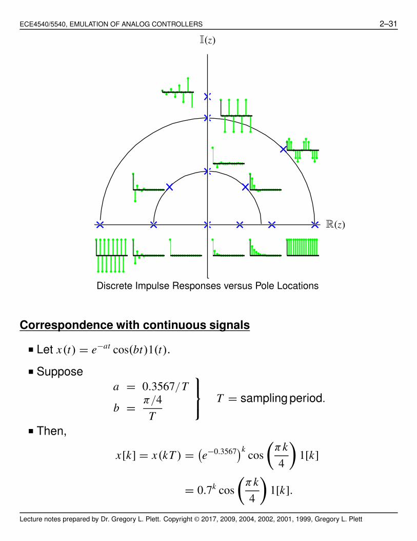
■ For a medium sampling rate, these compare as:


0

0

0

0.5ωp

0.5ωp

ωp

ωp

1.5ωp

1.5ωp

2ωp

2ωp

2.5ωp

2.5ωp0

0.5

1

−50−100−150−200−250

T = 1, ωs = 2π/1 = 2π , ωs = 6.3ωp

■ For a slow sampling rate, these compare as:


(system

0

0

0

0.5ωp

0.5ωp

ωp

ωp

1.5ωp

1.5ωp

2ωp

2ωp

2.5ωp

2.5ωp0

0.5

1

−50−100−150−200−250

T = 2, ωs = π , ωs = 3.14ωp

Zero-pole matching

■ There are other methods for emulating continuous-time systems with

discrete-time systems.

■ For example, we have seen before that if we take the z-transform of a

signal, the poles of the z-transform are related to the poles of the

s-transform via z = esT .



■ There was no direct mapping of zeros.

■ Now, we consider transforming a system. Rules:

1. Poles map as z = esT .

2. Finite zeros map as z = esT .

3. Zeros at ∞ (high freq.) map to z = −1 (high freq).

(but, may want to move one zero from z = −1 to ∞ to give

processing time: zero at ∞ = pole at 0 = 1/z = delay).

4. Match the gain of H(s) and H(z) at dc.

EXAMPLE: First method: move zero at ∞ to z = −1:

H(s) =a

s + a➠ pole at − a, zero at ∞

H(z) = kz + 1

z − e−aT.

■ Match at dc: Hs(0) = 1, Hz(1) =2k

1 − e−aT. . . k =

1 − e−aT

2.

H(z) =(z + 1)(1 − e−aT )

2(z − e−aT ).

EXAMPLE: Second method: move zero at ∞ to origin:

H(z) =k

(z − e−aT ).

■ Match at dc: Hs(0) = 1, Hz(1) =k

1 − e−aT. . . k = 1 − e−aT .

H(z) =(

1 − e−aT

z − e−aT

)

.

sysd=c2d(sys,T,'matched');



Hold equivalents

■ Two other methods I won’t discuss in detail.

■ ZOH: sysd=c2d(sys,T,’zoh’) H(z) =z − 1

zZ

{

H(s)

s

}

■ FOH: sysd=c2d(sys,T,’foh’) H(z) =(z − 1)2

T zZ

{

H(s)

s2

}

• The Z{·} notation will be explored in detail in Chapter 3.

■ System from pg. 2–41 revisited. . .

ctszohmatchedfoh

0

0

0

0.5ωp

0.5ωp

ωp

ωp

1.5ωp

1.5ωp

2ωp

2ωp

2.5ωp

2.5ωp0

0.5

1

1.5

−100

−200

−300

−400

T = 1, ωs = 2π/1 = π , ωs = 6.3ωp

ctszohmatchedfoh

0

0

0

0.5ωp

0.5ωp

ωp

ωp

1.5ωp

1.5ωp

2ωp

2ωp

2.5ωp

2.5ωp0

0.5

1

1.5

−200

−400

−600

−800

T = 2, ωs = 2π/2 = π , ωs = 3.14ωp



2.12: Design by emulation

■ These emulation techniques approximate an open-loop system D(s)

with an open-loop system D(z).

■ What happens when D(z) is placed in a feedback loop?

zohD2AA2D

D(z) G(s)Q

w(t)

v(t)

y(t)r (t)u(t)u[k]e(t) e[k]

■ We will look at this in more detail later.

■ Recall, though, that the biggest difference in performance will be due

to the T/2 second delay in the ZOH.

EXAMPLE:

G(s) =1

s(10s + 1).

■ Specifications for the design:

1. Mp < 16%.

2. ts < 10 s to 1%.

3. ess for ramp input < 0.01, slope of ramp = 0.01.

4. Sampling time to give ≥ 10 samples in rise time.

■ Step 1: Design D(s).

“1” ➠ ζ ≥ 0.5.

“2” ➠ σ ≥ 0.46.

“3” ➠ Kv =0.01

0.01= 1.0.



Choose D(s) to cancel plant pole approximately.

D(s) =10s + 1

s + 1.

−2 −1.5 −1 −0.5

1

−1

K = 1 . . . ➠ . . . Kv = 1 and good pole locations.

ωn ≈ 1 for pole locations, so tr ≈ 1.8 sec.

“4” T = tr/10 = 0.18 ➠ choose T = 0.2.

■ Step 2: D(s) ⇒ D(z): Use pole-zero matching.

• D(s) has zero at −1/10 ➠ D(z) has zero at z = e−0.1T .

• D(s) has pole at −1 ➠ D(z) has pole at z = e−T .

• D(s) has dc-gain 1 ➠ D(z) has dc-gain 1.

D(z) = K(z − 0.9802)

(z − 0.8187).

• DC-gain of D(z) = limz→1

D(z) = K(1 − 0.9802)

(1 − 0.8187). . . K = 9.15.

D(z) = 9.15(z − 0.9802)

(z − 0.8187).



Zero−OrderHold

ydisc

To Workspace2

udisc

To Workspace1

ycont

To Workspace

Sum1

SumStep

1

10s +s2

Plant2

1

10s +s2

Plant

9.15(z−0.9802)

(z−0.8187)

D(z)

10s+1

s+1

D(s)

(system dela

■ Try again, but with 1.0 sec sampling period.

D(z) = 6.64(z − 0.9048)

(z − 0.3679).

■ Much more overshoot, poorer damping.

0 5 10 15 20−0.5

0

0.5

1

1.5

Time (sec)

Outp

ut

u/10

Cont.

Disc.

Simulation for T = 0.2

0 5 10 15 20−0.5

0

0.5

1

1.5

Time (sec)

Outp

ut

u/10

Cont.

Disc.

Simulation for T = 1

Where to from here?

■ We have completed our look at design by emulation.

■ We now move in the direction of direct digital-control design.

■ First, we need to spend some time understanding the D2A and A2D

operations thoroughly.


Documents

EMULATION OF ANALOG CONTROLLERSmocha-java.uccs.edu/ECE5540/ECE5540-CH02.pdf · ECE4540/5540, EMULATION OF ANALOG CONTROLLERS 2–9 Performance not great, so tried again with T = 0.1ms.Much