Employment Effects of Unemployment InsuranceGenerosity During the Pandemic

Joseph Altonji, Zara Contractor, Lucas Finamor, Ryan Haygood,Ilse Lindenlaub, Costas Meghir, Cormac O’Dea,

Dana Scott, Liana Wang, and Ebonya WashingtonTobin Center for Economic Policy

Yale University ∗

July 14, 2020

Abstract

The CARES Act expanded unemployment insurance (UI) benefits by providing a $600weekly payment in addition to state unemployment benefits. Most workers thus became eligi-ble to receive unemployment benefits that exceed their weekly wages. It has been hypothesizedthat such high benefits encourage employers to lay off workers and discourage workers fromreturning to work. In this note, we test whether changes in UI benefit generosity are associatedwith decreased employment, both at the onset of the benefits expansion and as businesses lookto reopen. We use weekly data from Homebase, a private firm that provides scheduling andtime clock software to small businesses, which allows us to exploit high-frequency changesin state and federal policies to understand how firms and workers respond to policy changesin real time. Additionally, we benchmark our results from the Homebase data to employmentoutcomes in the Current Population Survey (CPS). We find that that the workers who experi-enced larger increases in UI generosity did not experience larger declines in employment whenthe benefits expansion went into effect. Additionally, we find that workers facing larger ex-pansions in UI benefits have returned to their previous jobs over time at similar rates as others.We find no evidence that more generous benefits disincentivized work either at the onset ofthe expansion or as firms looked to return to business over time. In future research, it will beimportant to assess whether the same results hold when states move to reopen, and to analyzethe effects of high UI replacement rates on reallocation of labor both within and across firms.

∗Dana Scott is the primary author of this report. We are very grateful to Homebase for making the data available forthis research and thank Ray Sandza and Andrew Vogeley at Homebase for assisting us in understanding the data. Weare also grateful to the Cowles Foundation and the Tobin Center for Economic Policy at Yale University for funding.Mistakes and opinions are our responsibility.

1

1 Introduction

The Coronavirus Aid, Relief, and Economic Stimulus (CARES) Act instituted a variety of eco-nomic policy responses to the Covid-19 pandemic. One such policy was a large, temporary ex-pansion of unemployment insurance (UI) benefits known as the Federal Pandemic UnemploymentCompensation (FPUC). The expansion provided a $600 weekly payment in addition to any stateunemployment benefits for which a worker would have already been eligible. The payment wasdesigned to replace 100 percent of the mean U.S. wage when combined with existing UI benefits.

When the CARES Act was passed, the UI expansion was set to continue until July 31, 2020.However, as the Coronavirus pandemic has continued into the summer, many states are experienc-ing surges in virus transmission as they move to reopen. Given the current public health context,policymakers are debating how best to provide social insurance against economic dislocations inthe pandemic. The current policy debate on expanded unemployment benefits is focused on bothwhether such expanded benefits should continue past their original expiration date and whether thefixed $600 payment is the appropriate form for such benefits to take.

Many academic, journalistic, and anecdotal sources have documented that the extra $600weekly payment provided under CARES yields a total UI benefit that is greater than weekly earn-ings when working for the median worker. This results from the fact that the earnings distributionin the U.S. is right-skewed, so the median worker earns less than mean earnings. Ganong et al.

(2020) estimate ex post replacement rates over 100 percent for 68 percent of unemployed workerswho are eligible for UI, as well as a median replacement rate of 134 percent. Given these factsabout the distribution of replacement rates, it is natural to ask whether such high replacement rates(a) encourage employers to lay off workers and (b) discourage workers from returning to workwhile they are still able to receive UI benefits.

In this note we build on previous work on UI replacement rates under the CARES Act to testwhether changes in UI benefit generosity are associated with decreased employment, both at theonset of the benefits expansion and as businesses look to return to work over time. We use data fromHomebase, a private firm that provides scheduling and time clock software to small businesses,which allows us to exploit high-frequency changes in state and federal policies to understand howfirms and workers respond to policy changes in real time. Many groups are studying the labormarket effects of the Covid-19 pandemic, several of which conduct exercises using the data fromHomebase. In particular, Bartik et al. (2020) analyze relationships between UI expansion in labormarket outcomes using Homebase data. We contribute to this developing literature in two ways.First, we propose a new measure to more effectively capture workers’ exposure to increased UIgenerosity. Namely, we measure the ratio of a worker’s post-CARES UI replacement rate to theirpre-CARES replacement rate. This has the effect of measuring the extent to which the FPUC

2

increased a worker’s unemployment benefits, rather than just measuring the generosity of benefitsonce the CARES Act became law. Second, we leverage this measure of treatment intensity in anevent study design to test whether the expansion of UI benefits decreased employment. To the bestof our knowledge, this note is the first to analyze the effect of differential changes to UI benefitgenerosity on employment.

We find that that the workers who differed in exposure to changes in UI generosity did notexperience different declines in employment from the week of March 22 – immediately prior tothe passage of the CARES Act – to any of the subsequent weeks. In fact, if anything, groupsfacing larger increases in benefit generosity experience slight gains in employment relative to theleast-treated group by early May. We show results from an event study that controls flexibly forthe severity of the Covid-19 pandemic as well as heterogeneous state-level business restrictions.We also perform a series of simplified comparisons between the week of March 22 to each of thesubsequent six weeks. Our results are robust to benchmarks using data from the Current PopulationSurvey (CPS). These results provide suggestive evidence that, in the aggregate, the expansion inUI benefit generosity did not disincentivize work at the outset, and that high replacement rates didnot differentially deter workers from returning to work.

2 Institutional background

2.1 UI benefits eligibility

While the CARES Act greatly expanded eligibility for unemployment insurance, several institu-tional features that restrict eligibility remained intact. In this section we discuss those features thatare directly relevant to the question of the effect of UI generosity on labor supply.

First, even under CARES, a worker who quits her job is ineligible for UI. While workers whoquit due to exceptional circumstances related to Covid-19 – e.g. having a respiratory conditionthat heightens one’s own risk or caring for an elderly relative – are exempted from this, those whoquit for no reason other than general concern about contracting Covid-19 are not eligible for UI.However, it is plausible that at small firms like the ones represented in Homebase, employers andworkers could cooperate to lay off workers who would receive higher incomes from UI benefitsthan from earned wages.

Second, once a person receives a “suitable offer of employment,” they are no longer eligiblefor UI even if they reject the offer. The Department of Labor specifically states that “a requestthat a furloughed employee return to his or her job very likely constitutes an offer of suitableemployment that the employee must accept” (U.S. Department of Labor (2020)). In practice, it islikely that compliance with this rule is determined by the level of formality of hiring and reporting

3

structures at a given firm; compliance may be lower at small firms where employers interact withworkers more informally. Additionally, this feature may lead to overestimates of re-employmentsince workers with an offer to return would face a stronger incentive to begin working again thanthose who would have to search for a job to become re-employed.

Together, these features of UI benefits eligibility suggest that if UI expansion decreases laborsupply through the mechanism described by critics, it is likely to do so to a greater extent at smallfirms than at large ones. It is particularly instructive, then, to test for such an effect in a sample ofsmall firms such as those represented in Homebase, because any observed effect could plausiblyserve as an upper bound for labor supply’s sensitivity to UI generosity.1

2.2 Timing of the CARES Act

On Thursday, March 19, 2020, Senate Republicans introduced a $1 trillion economic relief pack-age. The bill in its original form did not include supplemental unemployment insurance (Sullivan(19 March 2020)). News coverage of the progress of the bill indicates that legislators agreed to in-clude supplemental unemployment benefits on Monday, March 22 (Cochrane et al. (22 March2020)). The structure of unemployment benefits continued to be contested as the bill stalledthroughout the week, particularly over the issue of whether benefits would be extended for threemonths or four. The bill ultimately passed the Senate on Wednesday, March 25. It passed theHouse of Representatives on Thursday, March 26 and was signed into law on Friday, March 27.

The timing of events in the passage of the stimulus bill is important for the establishmentof employers’ and workers’ plausible responses to the policy intervention. Since supplementalunemployment insurance did not appear in the draft bill until Monday of the week in which it waspassed, and was contested in subsequent days, it is unlikely that employers or workers anticipatedenhanced unemployment benefits in their extensive-margin labor market decisions that week. Thatis, it is unlikely that the decision to open a firm in the week beginning March 21 or to lay offa worker prior to the start of work in that week could have been influenced by anticipation ofenhanced unemployment benefits.

Furthermore, as Ganong et al. (2020) note, the $600 size of the supplemental payment wasdesigned to replace 100 percent of the mean U.S. wage when combined with mean state UI ben-efits. Journalistic discourse about the supplemental insurance reflects this intention, rather thanthe practical effect of replacing more than 100 percent of median wages. For example, Cochraneand Fandos (23 March 2020) wrote on March 24, ”The two sides had previously agreed to expandthe program considerably, to include self-employed and part-time workers who traditionally havenot been eligible, and to cover 100 percent of wages to the average worker.” While there has been

1The effects of UI generosity on lost output, as opposed to employment, depend on the skill levels of those affectedas well as labor supply responses.

4

significant academic, journalistic, and anecdotal coverage of replacement rates above 100 percentsince the CARES Act passed, the timing of events and language used in the week leading up toits passage indicate that anticipation effects of replacement rates over 100 percent, at least on theextensive margin, are unlikely in the week beginning March 21.

3 Data and Sampling

3.1 Homebase

Homebase is a private firm that provides scheduling and time clock software to small businesses,covering a sample of hundreds of thousands of workers across the U.S. and Canada. Homebasehas made these data available to several teams of researchers. Further discussions of the Homebasedata can be found in Altonji et al. (2020), Bartik et al. (2020), Chetty et al. (2020), and Kurmannet al. (2020).

As other researchers have noted, the firms in the Homebase dataset are not representative ofthe entire US labor market. Homebase’s clients are primarily small firms that require time clocksfor their day-to-day operations, over half of which are in the food and drink industry. Addition-ally, workers in our sample of the data are hourly workers, not salaried employees.2 Because ofthese limitations, insights about the Homebase sample should not be viewed as representative ofthe entire labor market. Indeed, replication of this analysis on different and more representativesamples is an important area for future work. However, as Bartik et al. (2020) note, the popula-tion covered by Homebase is of particular policy interest since it represents a segment of the labormarket disproportionately affected by the pandemic. In the context of unemployment benefits gen-erosity, the Homebase sample is particularly valuable because it covers workers with relativelylow wages – most are in the first and second quintiles of national earnings as reported in the CPS.These workers experience relatively large changes in benefits generosity from the addition of the$600 supplemental payment compared to higher-earning workers. Therefore, we would expectour results from this sample to overestimate the effects of more generous benefits on labor marketresponses. That is, if there is no evidence of moral hazard in this group, there is unlikely to beany in a more representative sample. On the other hand, the drop in labor demand stemming fromthe decline in consumer demand and operating restrictions were especially pronounced in the foodand drink industry. This would have made moral hazard less relevant.

In addition to the sample selection caveats, the Homebase data is subject to some additionallimitations. Notably, workers who have been furloughed (i.e. are still employed by a firm but

2While some firms list their salaried employees in the data (primarily managers), their wages are coded at zero andthey do not clock in and out. Since Homebase’s software is not designed to consistently track these workers’ earnings,we exclude them from our analysis.

5

are not working any hours) are not distinguishable from workers who have been formally laid off.In the context of labor market responses to changes in unemployment insurance generosity, thisdistinction is important. For instance, consider a firm that furloughs its employees at t = 1 when astate mandates that the firm shut down, but then moves to lay off some or all of its workers at t = 2when the unemployment insurance available to its employees increases substantially. We wouldnot be able to observe the layoff at t = 2 and would code the workers’ exit from the firm as a layoffat t = 1. While this data limitation will lead us to underestimate the effect of changes in unemploy-ment benefit generosity on employment, this effect is mitigated by the specific policy implicationsin which we are interested. Namely, we aim to understand the implications of generous UI benefitsfor workers’ choices between paid work and unemployment in which they receive UI. As states be-gin to reopen and policymakers consider whether increased UI generosity disincentivizes workersfrom returning to productive work, the choice between UI benefits and furlough is not of particularimportance.

3.2 Current Population Survey (CPS)

We supplement our results from the Homebase data with benchmarks from the Current PopulationSurvey (CPS), a more representative sample of the US labor market. The CPS is administeredmonthly and asks about labor market activities in the second week of a given month. Participantsrespond to the CPS for a period of 4 consecutive months, then rotate out for 8 months, then rotateback in for another period of 4 consecutive months before rotating out permanently. For example,a respondent in our sample may be in the data in February, March, April, And May 2019; theywould then rotate in for February, March, April, and May 2020 before rotating out permanently.

While the CPS is administered monthly, the reference-week structure allows us to exploit spe-cific questions about employment to impute weekly employment data in weeks between surveys.We observe respondents in the CPS in the weeks of February 9, March 8, April 12, and May 10.We impute employment in the intervening weeks as follows. If a respondent is employed in boththe first and second month, we code them as employed in all intervening weeks. If a respondentis unemployed in both the first and second month, we code them as unemployed in all interveningweeks. If a respondent is employed in the first week and unemployed in the second, we use thenumber of weeks of continuous unemployment reported in the second month’s survey to imputethe week in which she became unemployed. If a respondent is unemployed in the first week andemployed in the second week, we exclude her from the sample in the intervening weeks. Thatis, she will appear in the weeks in which she was surveyed, but we drop her from the interveningweeks because we cannot observe in which week she became employed.

In our preferred specification we classify a respondent as employed if she was at work in the

6

reference week or if she reports that she has a job but was not at work in the reference week. Thismeans that we may count as employed some workers who were on furlough, who would havebeen counted as unemployed in the Homebase data as described in section 3.1. Our definition ofemployment in the CPS is consistent with eligibility requirements for UI (i.e. a person cannot beemployed, but furloughed, and receive UI). However, this means that employment levels in theCPS data will tend to be higher than those in the Homebase data. We expect that, if furlough ratesdiffer across replacement rate ratio categories, they are if anything likely to be lower among thosefacing more generous UI. To verify this, we show additional results in Appendix Figure 1 andAppendix Table 1 in which we define as unemployed any worker who reports that they had a jobbut were not at work in the reference week. Our results in the CPS are robust to this alternativedefinition.

3.3 UI benefits calculator

We compute pre- and post-CARES UI benefit replacement rates using the calculator developed byGanong et al. (2020). To compute an individual’s eligibility for unemployment benefits, all statesmake use of a worker’s four-quarter earning history. Most states compute benefits as a percentageof the worker’s highest quarter earnings, second-highest quarter earnings, or annual earnings in thefour most recent completed quarters prior to filing, subject to a minimum and maximum benefitlevel. In our case, to compute UI benefits, we use workers’ earnings histories in the four completedquarters of 2019.

To improve precision in our simulations of individuals’ UI benefits, we restrict our Homebasesample to only those workers who worked at a given firm for at least 10 weeks in each quarter atan average of at least 30 hours in each week worked – that is, only those workers who worked full-time at Homebase firms for all of 2019. Since we only observe an individual’s work history whentheir firm is in the Homebase data, this restriction aims to exclude individuals who worked in otherjobs during the period over which UI benefits are calculated, either in a full-time capacity prior totheir employment at the Homebase member firm or in a part-time capacity concurrently with theiremployment at the Homebase member firm. In addition, we further restrict our sample to workerswho: (1) worked at least 16 hours in the base period, defined as the two weeks from January 19 toFebruary 1; (2) worked at a firm in the base period that recorded at least 40 worker-hours duringthat period; and worked at the same firm both throughout 2019 and during the base period.

We note that by imposing this restriction we necessarily exclude the shortest-tenured workers ata given firm, as well as workers at newly established firms. It is plausible that our sampled workersare less likely to be laid off in an economic downturn than shorter-tenured workers. Furthermore,firms established in the last year may be more likely to shut down than longer-running ones. This

7

selection problem may lead us to underestimate the effect of UI expansion on employment. How-ever, while excluded workers and firms may be more sensitive to the economic shock imposed bythe pandemic, conditional on wages there is no a priori reason to believe that they will be morelikely to lay off workers in response to the change in unemployment benefits in particular.

In the CPS data, we impose sampling restrictions to be able to compute UI benefits. To com-pute benefits, as described in section 3.3, we need to observe quarterly earnings history, which isnot available in the monthly CPS. We thus restrict our sample to respondents in the 2020 CPS whoanswered the 2019 CPS Annual Social and Economic Supplement (ASEC). The 2019 ASEC is ad-ministered in February, March, and April of 2019 and asks about labor market activities in calendaryear 2018. Following Ganong et al. (2020), we restrict our analysis to 2019 ASEC respondentswho (1) are US citizens, (2) report hourly earnings in the ASEC of at least the federal minimumwage of $7.25, and (3) would have been eligible for UI benefits prior to the passage of the CARESAct in their state of residence on the basis of their 2018 earnings. Additionally, to ensure that weare comparing similar outcomes in the CPS and in Homebase, we further restrict our sample toworkers who were employed as of the February 2020 survey.

3.4 State policies and Covid-19 incidence

To track start and end dates of various state-level restrictions in response to the pandemic, we usethe COVID-19 US state policy database (CUSP) maintained by Raifman et al. (2020). We usethree types of restrictions. First, we use stay-at-home orders, which restrict people’s movementoutside the home to visits to essential businesses and public services. Second, we use requiredclosure of non-essential businesses as a proxy for restrictions on business activity. Third, we userestrictions of restaurants to takeout-only, which is of particular value in our data set given thesubstantial overrepresentation of bars and restaurants in our sample. Fourth, we use mandatoryclosures of gyms, since these saw particularly stringent shutdown requirements and there are manyHomebase firms in the health and fitness industry. Additionally, we use data on new Covid-19cases per capita from the Johns Hopkins University Center for Systems Science and Engineering(CSSE) to measure the severity of the pandemic in each state.

4 Empirical approach

4.1 Measurement of UI benefits generosity

The UI replacement rate is determined by two inputs: first, the individual’s earnings history fromthe four prior completed quarters; and second, their state’s schedule of benefits. When studying

8

the effects and policy implications of changes to the UI replacement rate, it is important to notethat the variation in treatment comes not from the replacement rate per se, but from the change inbenefits generosity that results from the CARES Act. For individual i in state s the replacementrate under CARES is given by:

replCARES,is =UICARES,is

w2019,is=

UI2019,is +600w2019,is

= repl2019,is +600

w2019,is(1)

where UI2019,is is the benefit amount for which they would have been eligible in January 2020and w2019,is is the average weekly wage in 2019, the reference period for calculating UI benefits.The variation we aim to exploit comes from the differential change in replacement rates from theincremental $600. To measure increases in UI generosity, we compute the ratio of an individual’sreplacement rate under CARES to their replacement rate prior to CARES. We refer to this measureas the replacement rate ratio for worker i in state s:

ris =replCARES,is

repl2019,is=

UICARES,is

UI2019,is= 1+

600UI2019,is

(2)

Using this measure instead of the raw replacement rate has the effect of directly measuring thechange in UI generosity rather than either the ex ante or ex post generosity. See Table 4 for anillustrative example of how replacement rates are determined by both state-level benefit generosityand workers’ wages. We note that using this measure does not in itself resolve the central endo-geneity problem inherent in studying replacement rates. Since the replacement rate ratio is stillcorrelated with workers’ wages, we control for wages in our main specification. However, futurework should explore alternative identification strategies to address wage endogeneity.

4.2 Event study

To analyze the effects of the passage of the CARES Act on employment for workers facing differentchanges to UI benefits generosity, we show results from a linear probability event study model. Weestimate the probability of employment for individual i in replacement ratio group g, industry j,state k, at time t

yig jkt = ∑s 6=3

αs1{s = t}+∑b

βb1{b = g}+

∑s 6=3

∑b

γb,s1{b = g}1{s = t}+ ∑s 6=3

δsig jk1{s = t}Xig jk + εig jkt (3)

where 1{s = t} is a full set of week dummies, 1{b = g} are dummies indicating membership inreplacement ratio group g, and Xig jk is a vector of controls containing pre-CARES replacement

9

rate, baseline wage, and industry in the baseline specification. In an additional specification weadd time-varying controls for (a) new Covid-19 cases per capita reported in a given state-weekand (b) indicators for whether states had active policies of each of the following types in a givenweek: stay-at-home orders, mandatory closures of non-essential businesses, mandatory closures ofrestaurants except for takeout, and mandatory closures of gyms. In all specifications we allow theeffect of the controls to vary over time by interacting them with the full set of week dummies.3

5 Results

Figure 2 plots the γgt coefficients on the interaction between the week indicators t and the replace-ment rate ratio bins g in equation 3. Conceptually, the coefficients indicate the change in probabil-ity of employment relative to the reference group in a given week. The reference group is definedas workers who have a replacement rate ratio less than 2.5, i.e. workers whose replacement rateincreases by less than 150 percent. The base period is defined as the two weeks from January 19to February 1. The outcome variable of interest is an indicator for employment. We code a workeras employed when they record nonzero hours in a given week. We control for industry, baselinereplacement rate, baseline wage in both panels. In panel (b) we add controls for the number of newcases of Covid-19, and whether the state had instituted each of the following business restrictions:(1) stay-at-home order, (2) mandatory closure of non-essential businesses, (3) mandatory closureof restaurants except for takeout service, and (4) mandatory closure of gyms. The shaded areasaround each line represent 90% confidence intervals.

The figure shows that the workers who differed in exposure to changes in UI generosity didnot experience different declines in employment from the week of March 22 – immediately priorto the passage of the CARES Act – to any of the subsequent weeks. While the workers withthe largest changes in UI generosity experience the largest declines in employment relative to theJanuary baseline, the differential decline occurs entirely in the weeks prior to the passage of theCARES Act. As discussed in section 2.2 it is unlikely that firms and workers could have acted inanticipation of expanded UI replacement rates, so the null result comparing the week of March 22to subsequent weeks is the relevant one to assess. Furthermore, the figure suggests that workerswith larger increases in benefit generosity are no slower to return to work than others with moremodest UI increases.

If there were an aggregate negative effect of incremental UI generosity on employment atHomebase firms, one would expect to observe two patterns: (1) a significant drop in relative em-

3We obtain qualitatively similar results using a logit model of the probability of employment. We also obtainqualitatively similar results when we measure the change in UI generosity using the difference replCARES,is−repl2019,israther than the replacement rate ratio ris.

10

ployment from the week of March 22 (immediately prior to the passage of CARES) to the first fullweek in which the Act was law (March 29) and (2) decreases in relative employment over timeas workers with more-generous UI expansions were slower to return to work over time. Even if,as has been documented, many states experienced implementation delays for several weeks after-ward, we could expect at least some drop in the first full week and a significant drop relative to thebaseline once all states had implemented the expanded UI benefits, when controlling for variationin states’ business operation restrictions over time. However, figure 2 shows no drop at all afterthe passage of CARES – if anything there appears to be a small, though statistically insignificant,increase in employment in the early weeks. Furthermore, workers facing larger UI expansionsappear to be quicker to return to work than others, not slower. While they do not fully catch up topre-Covid levels of relative employment conditional on controls, the gap has diminished over time.This serves as suggestive evidence against concerns that UI generosity disincentivizes returns towork.

Figure 3 shows that these results are robust to the CPS data. While there appears to be a small,but insignificant, drop in employment following the passage of the CARES Act, this is mitigatedby controlling for state-level business restrictions and new Covid-19 cases. Furthermore, workersfacing larger UI expansions generally appear to be quicker to return to work than others, not slower(though the group with replacement rate ratios of 3.0-3.5 is an exception). While they do not fullycatch up to pre-Covid levels of relative employment conditional on controls, the gap has diminishedover time. This provides corroborating evidence of our main result in the Homebase data.

We supplement the graphical evidence with a series of simplified DiD linear probability modelsto estimate the effect of increased UI generosity on employment by comparing employment inthe week of March 22, immediately prior to the passage of the CARES Act, to each of the sixsubsequent weeks. We compare to each of the following six weeks to account for the fact thatmany states experienced implementation delays in expanding their UI systems. We use the samecontrols as in the main specification. Standard errors are clustered at the worker level.

Table 5 shows that in each two-way comparison, an increase in replacement rate ratio is as-sociated with an increase in employment relative to the week immediately prior to the passage ofthe CARES Act. In the first three weeks, the replacement rate ratio is associated with a small andinsignificant decrease in employment relative to the week of March 22; however, the coefficientsare positive and insignificant in the fourth and fifth weeks, and positive and significant in the weekof May 3. Column (1) reports effects of the replacement rate ratio on employment is 0.003 lower inthe week of March 29 than it was in the week of March 22. In the week of May 3, the effect of thereplacement rate ratio on employment is 0.019 higher than it was in the week of March 22. In earlyweeks the relative differences in employment are economically small and statistically insignificant,but in the week of May 3 higher replacement rate ratios predict a higher rate of employment. Table

11

6 shows that there is not a significant difference by replacement rate ratio in employment relativeto the week immediately prior to the passage of the CARES Act for workers in the CPS sample.All reported coefficients are economically small and statistically insignificant.

Together, these results provide suggestive evidence that, in the aggregate, expansions in UIbenefit generosity did not disincentivize work at Homebase firms or for workers in the CPS, eitherat the onset of the expansion or as firms looked to return to business over time. This is consistentwith descriptive evidence in Bartik et al. (2020) and diminishes concerns that replacement ratessignificantly above 100 percent could cause a decline in labor supply or discourage workers fromreturning to work.

6 Conclusion

As policymakers consider whether to extend the expansion of UI generosity past its initial July 31expiration date, it is important to holistically consider the economic and public health impacts ofsuch a policy. This note provides preliminary evidence that expansions in UI replacement ratesdid not increase layoffs at the outset of the pandemic or discourage workers from returning to theirjobs over time. We note that our results do not necessarily imply that such responses do not exist –rather, they suggest that expanding UI generosity has not depressed employment in the aggregate.As many states struggle with surges in Covid-19 cases as they move to reopen, there are still goodreasons to not incentivize everyone to return to work and to continue to support displaced workersregardless of the labor market effects of such social insurance. However, we find no evidence tosupport concerns about adverse aggregate labor supply effects of expanded UI generosity in thecontext of the current pandemic.

We qualify our work with several caveats. First, it is impossible to directly estimate the extentto which firms and workers chose not to work as a result of UI expansion, since the effect is offsetby the economic stimulus of income expansion that indirectly boosts employment. However, in theaggregate, there is no evidence that the present UI expansion has decreased employment. Finally,our specification does not account for possible confounding effects. While we do control for Covid-19 cases as a proxy for the severity of the pandemic in each state, as well as for state businessrestrictions, there could be additional sources of unobserved state-level variation in employmentoutcomes that we do not account for here. Future research might explore alternative identificationstrategies to attempt to address this issue.

We emphasize that our results do not speak to the disemployment effects of UI generosityduring more normal times, which is the subject of a vast literature (Schmieder and von Wachter(2016)). The severity of the decline in labor demand and the health risks to workers make thecurrent pandemic different. Rather, our results offer a first step toward understanding the causal

12

dynamics of UI incentives in the context of the current pandemic. We propose to expand ourwork here in a few ways. First, future work should test for similar effects using event studiesaround states’ reopenings to assess whether workers with larger expansions in UI generosity areless likely to return to work when business restrictions are loosened. Second, we propose to extendour analysis to study firm-level employment to shed light on firms’ ability to hire workers to theirdesired capacity, whether those workers had previously been employed at the firm or not.

Additionally, future work on expanded UI generosity under the CARES Act will have impor-tant implications for the reallocation of labor during the pandemic. It has been hypothesized thatdisincentivizing people from going back to work may hinder reallocation in the labor market. Bar-rero et al. (2020) note that there are many businesses with both net and gross hiring. While ourinitial event study shows some suggestive evidence that firms in Homebase are in fact rehiring ex-isting workers, and that UI generosity does not predict slower rates of rehiring in either Homebaseor the CPS sample, further work to test the effects of expanded UI generosity on (a) whether firmschange the headcount or composition of their workforces and (b) whether laid-off workers moveto new jobs will be valuable.

13

ReferencesALTONJI, J., CONTRACTOR, Z., FINAMOR, L., HAYGOOD, R., LINDENLAUB, I., MEGHIR,

C., O’DEA, C., SCOTT, D., WANG, L. and WASHINGTON, E. (2020). The Effects of theCoronavirus on Hours of Work in Small Businesses, Yale Tobin Center for Economic Policy,June 11.

BARRERO, J. M., BLOOM, N. and DAVIS, S. J. (2020). COVID-19 Is Also a Reallocation Shock,Working Paper, June 5.

BARTIK, A. W., BERTRAND, M., LIN, F., ROTHSTEIN, J. and UNRATH, M. (2020). Measuringthe labor market at the onset of the COVID-19 crisis. Brookings Papers on Economic Activity,June 25.

CAJNER, T., CRANE, L. D., DECKER, R. A., GRIGSBY, J., HAMINS-PUERTOLAS, A., HURST,E., KURZ, C. and YILDIRMAZ, A. (2020). The U.S. labor market during the beginning of thepandemic recession, Working paper, June 14.

CHETTY, R., FRIEDMAN, J. N., HENDREN, N., STEPNER, M. and THE OPPORTUNITY IN-SIGHTS TEAM (2020). How did COVID-19 and stabilization policies affect spending and em-ployment? A new real-time economic tracker based on private sector data, Working paper, June17.

COCHRANE, E. and FANDOS, N. (23 March 2020). Top Senate Democrat and Treasury SecretarySay They Are Near a Stimulus Deal. The New York Times.

— and — (24 March 2020). Democrats Near Deal With White House on Stimulus Package. TheNew York Times.

—, TANKERSLEY, J. and SMIALEK, J. (22 March 2020). Emergency Economic Rescue Plan inLimbo as Democrats Block Action. The New York Times.

GANONG, P., NOEL, P. and VAVRA, J. (2020). US Unemployment Insurance Replacement RatesDuring the Pandemic, Becker Friedman Institute Working Paper 2020-62, May.

HULSE, C. (21 March 2020). Push for Cash in Rescue Package Came From Unlikely Source:Conservatives. The New York Times.

JOHNS HOPKINS UNIVERSITY CENTER FOR SYSTEMS SCIENCE AND ENGINEERING(CSSE) (2020). 2019 Novel Coronavirus Visual Dashboard. https://github.com/CSSEGISandData/.

KURMANN, A., LALE, E. and TA, L. (2020). The impact of COVID-19 on U.S. employment andhours: Real-time estimates with Homebase data, Working paper, May.

RAIFMAN, J., NOCKA, K., JONES, D., BOR, J., LIPSON, S., JAY, J. and CHAN, P. (2020).COVID-19 US state policy database. www.tinyurl.com/statepolicies.

SCHMIEDER, J. F. and VON WACHTER, T. (2016). The Effects of Unemployment Insurance Ben-efits: New Evidence and Interpretation. Annual Review of Economics, 8 (1), 547–581.

SULLIVAN, E. (19 March 2020). 5 Takeaways From the Coronavirus Economic Relief Package.The New York Times.

U.S. DEPARTMENT OF LABOR (2020). Unemployment Insurance Relief During COVID-19 Out-break. https://www.dol.gov/coronavirus/unemployment-insurance.

14

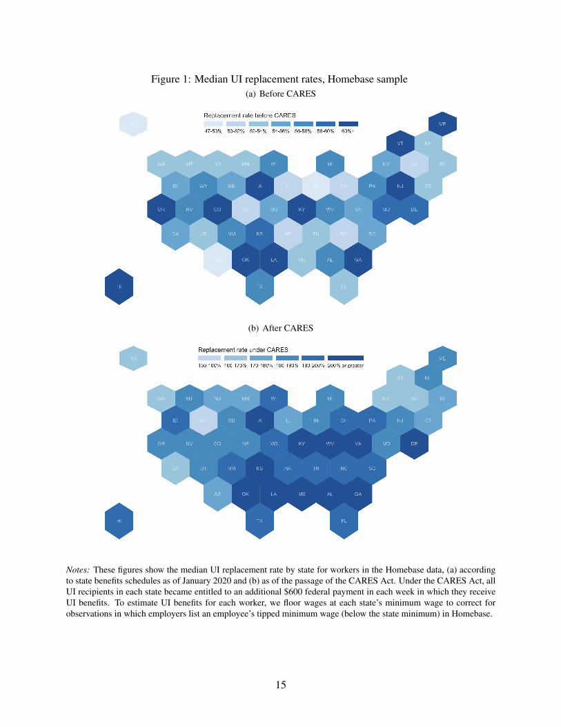
Figure 1: Median UI replacement rates, Homebase sample(a) Before CARES

(b) After CARES

Notes: These figures show the median UI replacement rate by state for workers in the Homebase data, (a) accordingto state benefits schedules as of January 2020 and (b) as of the passage of the CARES Act. Under the CARES Act, allUI recipients in each state became entitled to an additional $600 federal payment in each week in which they receiveUI benefits. To estimate UI benefits for each worker, we floor wages at each state’s minimum wage to correct forobservations in which employers list an employee’s tipped minimum wage (below the state minimum) in Homebase.

15

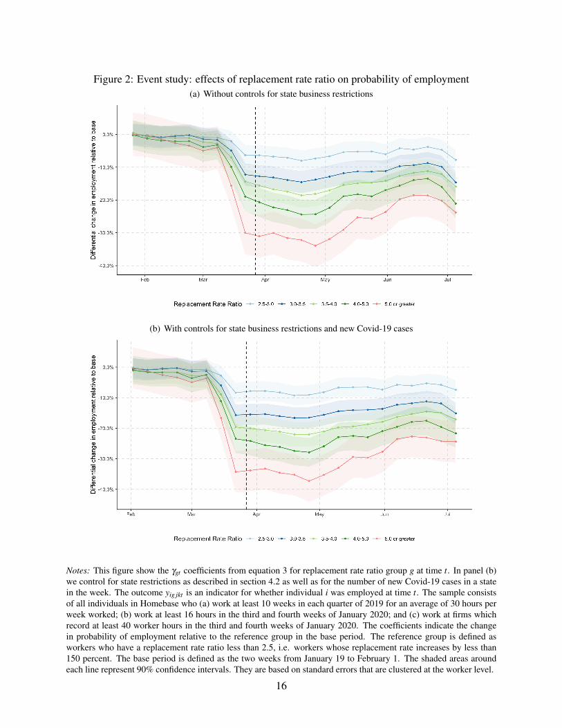
Figure 2: Event study: effects of replacement rate ratio on probability of employment(a) Without controls for state business restrictions

(b) With controls for state business restrictions and new Covid-19 cases

Notes: This figure show the γgt coefficients from equation 3 for replacement rate ratio group g at time t. In panel (b)we control for state restrictions as described in section 4.2 as well as for the number of new Covid-19 cases in a statein the week. The outcome yig jkt is an indicator for whether individual i was employed at time t. The sample consistsof all individuals in Homebase who (a) work at least 10 weeks in each quarter of 2019 for an average of 30 hours perweek worked; (b) work at least 16 hours in the third and fourth weeks of January 2020; and (c) work at firms whichrecord at least 40 worker hours in the third and fourth weeks of January 2020. The coefficients indicate the changein probability of employment relative to the reference group in the base period. The reference group is defined asworkers who have a replacement rate ratio less than 2.5, i.e. workers whose replacement rate increases by less than150 percent. The base period is defined as the two weeks from January 19 to February 1. The shaded areas aroundeach line represent 90% confidence intervals. They are based on standard errors that are clustered at the worker level.

16

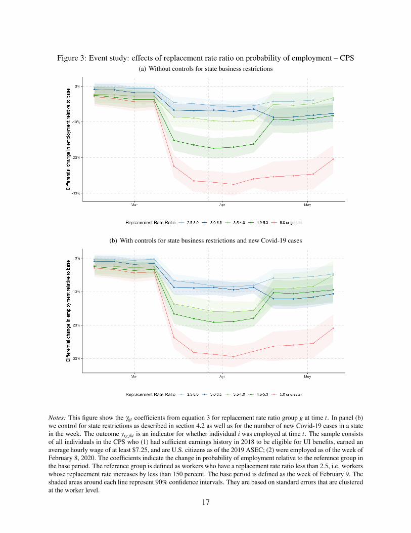
Figure 3: Event study: effects of replacement rate ratio on probability of employment – CPS(a) Without controls for state business restrictions

(b) With controls for state business restrictions and new Covid-19 cases

Notes: This figure show the γgt coefficients from equation 3 for replacement rate ratio group g at time t. In panel (b)we control for state restrictions as described in section 4.2 as well as for the number of new Covid-19 cases in a statein the week. The outcome yig jkt is an indicator for whether individual i was employed at time t. The sample consistsof all individuals in the CPS who (1) had sufficient earnings history in 2018 to be eligible for UI benefits, earned anaverage hourly wage of at least $7.25, and are U.S. citizens as of the 2019 ASEC; (2) were employed as of the week ofFebruary 8, 2020. The coefficients indicate the change in probability of employment relative to the reference group inthe base period. The reference group is defined as workers who have a replacement rate ratio less than 2.5, i.e. workerswhose replacement rate increases by less than 150 percent. The base period is defined as the week of February 9. Theshaded areas around each line represent 90% confidence intervals. They are based on standard errors that are clusteredat the worker level.

17

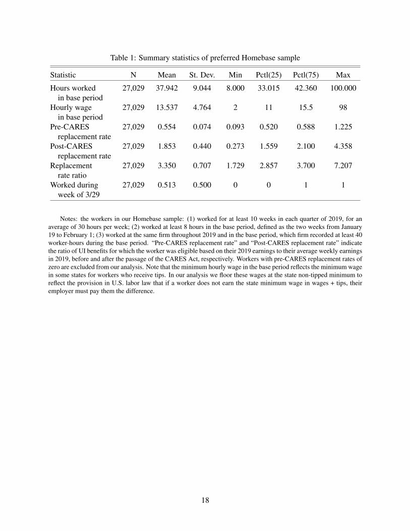
Table 1: Summary statistics of preferred Homebase sample

Statistic N Mean St. Dev. Min Pctl(25) Pctl(75) Max

Hours worked 27,029 37.942 9.044 8.000 33.015 42.360 100.000in base period

Hourly wage 27,029 13.537 4.764 2 11 15.5 98in base period

Pre-CARES 27,029 0.554 0.074 0.093 0.520 0.588 1.225replacement rate

Post-CARES 27,029 1.853 0.440 0.273 1.559 2.100 4.358replacement rate

Replacement 27,029 3.350 0.707 1.729 2.857 3.700 7.207rate ratio

Worked during 27,029 0.513 0.500 0 0 1 1week of 3/29

Notes: the workers in our Homebase sample: (1) worked for at least 10 weeks in each quarter of 2019, for anaverage of 30 hours per week; (2) worked at least 8 hours in the base period, defined as the two weeks from January19 to February 1; (3) worked at the same firm throughout 2019 and in the base period, which firm recorded at least 40worker-hours during the base period. “Pre-CARES replacement rate” and “Post-CARES replacement rate” indicatethe ratio of UI benefits for which the worker was eligible based on their 2019 earnings to their average weekly earningsin 2019, before and after the passage of the CARES Act, respectively. Workers with pre-CARES replacement rates ofzero are excluded from our analysis. Note that the minimum hourly wage in the base period reflects the minimum wagein some states for workers who receive tips. In our analysis we floor these wages at the state non-tipped minimum toreflect the provision in U.S. labor law that if a worker does not earn the state minimum wage in wages + tips, theiremployer must pay them the difference.

18

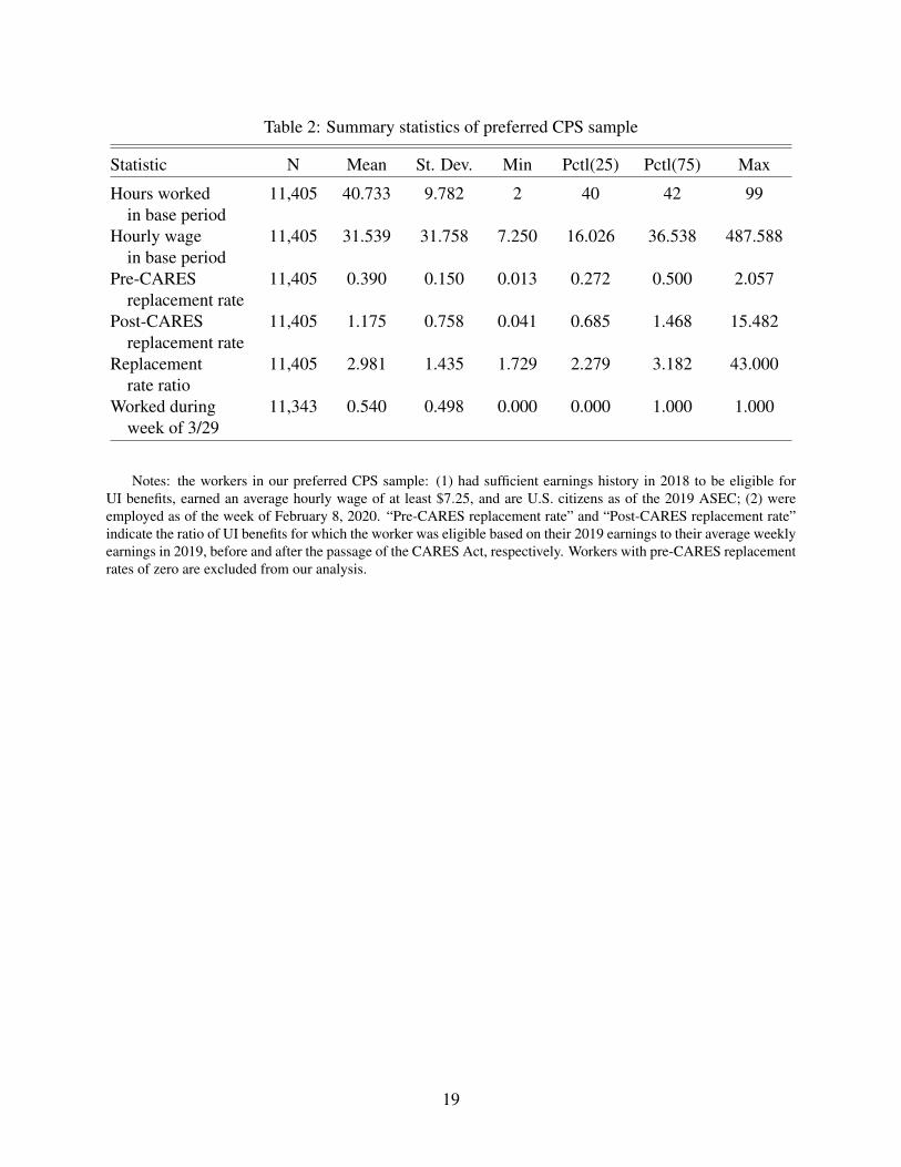
Table 2: Summary statistics of preferred CPS sample

Statistic N Mean St. Dev. Min Pctl(25) Pctl(75) Max

Hours worked 11,405 40.733 9.782 2 40 42 99in base period

Hourly wage 11,405 31.539 31.758 7.250 16.026 36.538 487.588in base period

Pre-CARES 11,405 0.390 0.150 0.013 0.272 0.500 2.057replacement rate

Post-CARES 11,405 1.175 0.758 0.041 0.685 1.468 15.482replacement rate

Replacement 11,405 2.981 1.435 1.729 2.279 3.182 43.000rate ratio

Worked during 11,343 0.540 0.498 0.000 0.000 1.000 1.000week of 3/29

Notes: the workers in our preferred CPS sample: (1) had sufficient earnings history in 2018 to be eligible forUI benefits, earned an average hourly wage of at least $7.25, and are U.S. citizens as of the 2019 ASEC; (2) wereemployed as of the week of February 8, 2020. “Pre-CARES replacement rate” and “Post-CARES replacement rate”indicate the ratio of UI benefits for which the worker was eligible based on their 2019 earnings to their average weeklyearnings in 2019, before and after the passage of the CARES Act, respectively. Workers with pre-CARES replacementrates of zero are excluded from our analysis.

19

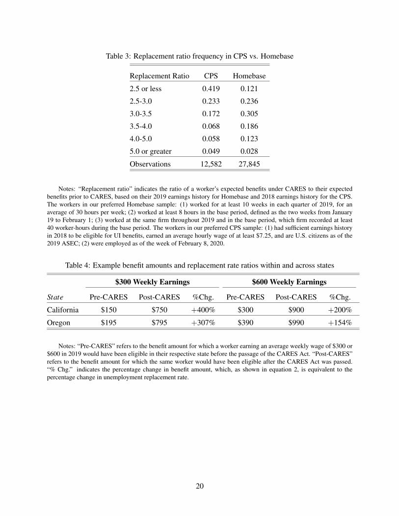
Table 3: Replacement ratio frequency in CPS vs. Homebase

Replacement Ratio CPS Homebase

2.5 or less 0.419 0.121

2.5-3.0 0.233 0.236

3.0-3.5 0.172 0.305

3.5-4.0 0.068 0.186

4.0-5.0 0.058 0.123

5.0 or greater 0.049 0.028

Observations 12,582 27,845

Notes: “Replacement ratio” indicates the ratio of a worker’s expected benefits under CARES to their expectedbenefits prior to CARES, based on their 2019 earnings history for Homebase and 2018 earnings history for the CPS.The workers in our preferred Homebase sample: (1) worked for at least 10 weeks in each quarter of 2019, for anaverage of 30 hours per week; (2) worked at least 8 hours in the base period, defined as the two weeks from January19 to February 1; (3) worked at the same firm throughout 2019 and in the base period, which firm recorded at least40 worker-hours during the base period. The workers in our preferred CPS sample: (1) had sufficient earnings historyin 2018 to be eligible for UI benefits, earned an average hourly wage of at least $7.25, and are U.S. citizens as of the2019 ASEC; (2) were employed as of the week of February 8, 2020.

Table 4: Example benefit amounts and replacement rate ratios within and across states

$300 Weekly Earnings $600 Weekly Earnings

State Pre-CARES Post-CARES %Chg. Pre-CARES Post-CARES %Chg.

California $150 $750 +400% $300 $900 +200%

Oregon $195 $795 +307% $390 $990 +154%

Notes: “Pre-CARES” refers to the benefit amount for which a worker earning an average weekly wage of $300 or$600 in 2019 would have been eligible in their respective state before the passage of the CARES Act. “Post-CARES”refers to the benefit amount for which the same worker would have been eligible after the CARES Act was passed.“% Chg.” indicates the percentage change in benefit amount, which, as shown in equation 2, is equivalent to thepercentage change in unemployment replacement rate.

20

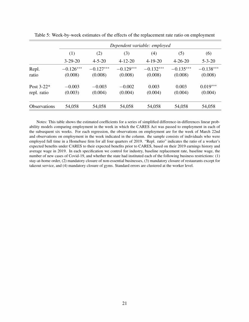
Table 5: Week-by-week estimates of the effects of the replacement rate ratio on employment

Dependent variable: employed

(1) (2) (3) (4) (5) (6)

3-29-20 4-5-20 4-12-20 4-19-20 4-26-20 5-3-20

Repl. −0.126∗∗∗ −0.127∗∗∗ −0.129∗∗∗ −0.132∗∗∗ −0.135∗∗∗ −0.138∗∗∗

ratio (0.008) (0.008) (0.008) (0.008) (0.008) (0.008)

Post 3-22* −0.003 −0.003 −0.002 0.003 0.003 0.019∗∗∗

repl. ratio (0.003) (0.004) (0.004) (0.004) (0.004) (0.004)

Observations 54,058 54,058 54,058 54,058 54,058 54,058

Notes: This table shows the estimated coefficients for a series of simplified difference-in-differences linear prob-ability models comparing employment in the week in which the CARES Act was passed to employment in each ofthe subsequent six weeks. For each regression, the observations on employment are for the week of March 22ndand observations on employment in the week indicated in the column. the sample consists of individuals who wereemployed full time in a Homebase firm for all four quarters of 2019. “Repl. ratio” indicates the ratio of a worker’sexpected benefits under CARES to their expected benefits prior to CARES, based on their 2019 earnings history andaverage wage in 2019. In each specification we control for industry, baseline replacement rate, baseline wage, thenumber of new cases of Covid-19, and whether the state had instituted each of the following business restrictions: (1)stay-at-home order, (2) mandatory closure of non-essential businesses, (3) mandatory closure of restaurants except fortakeout service, and (4) mandatory closure of gyms. Standard errors are clustered at the worker level.

21

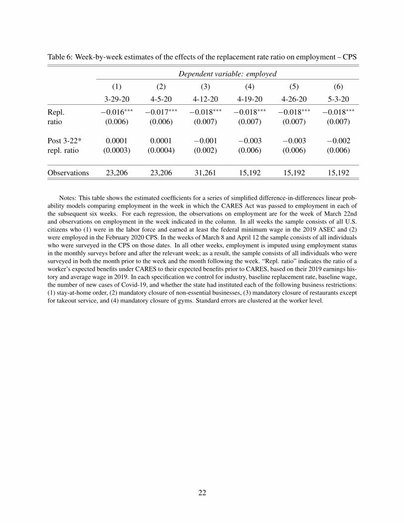
Table 6: Week-by-week estimates of the effects of the replacement rate ratio on employment – CPS

Dependent variable: employed

(1) (2) (3) (4) (5) (6)

3-29-20 4-5-20 4-12-20 4-19-20 4-26-20 5-3-20

Repl. −0.016∗∗∗ −0.017∗∗∗ −0.018∗∗∗ −0.018∗∗∗ −0.018∗∗∗ −0.018∗∗∗

ratio (0.006) (0.006) (0.007) (0.007) (0.007) (0.007)

Post 3-22* 0.0001 0.0001 −0.001 −0.003 −0.003 −0.002repl. ratio (0.0003) (0.0004) (0.002) (0.006) (0.006) (0.006)

Observations 23,206 23,206 31,261 15,192 15,192 15,192

Notes: This table shows the estimated coefficients for a series of simplified difference-in-differences linear prob-ability models comparing employment in the week in which the CARES Act was passed to employment in each ofthe subsequent six weeks. For each regression, the observations on employment are for the week of March 22ndand observations on employment in the week indicated in the column. In all weeks the sample consists of all U.S.citizens who (1) were in the labor force and earned at least the federal minimum wage in the 2019 ASEC and (2)were employed in the February 2020 CPS. In the weeks of March 8 and April 12 the sample consists of all individualswho were surveyed in the CPS on those dates. In all other weeks, employment is imputed using employment statusin the monthly surveys before and after the relevant week; as a result, the sample consists of all individuals who weresurveyed in both the month prior to the week and the month following the week. “Repl. ratio” indicates the ratio of aworker’s expected benefits under CARES to their expected benefits prior to CARES, based on their 2019 earnings his-tory and average wage in 2019. In each specification we control for industry, baseline replacement rate, baseline wage,the number of new cases of Covid-19, and whether the state had instituted each of the following business restrictions:(1) stay-at-home order, (2) mandatory closure of non-essential businesses, (3) mandatory closure of restaurants exceptfor takeout service, and (4) mandatory closure of gyms. Standard errors are clustered at the worker level.

22

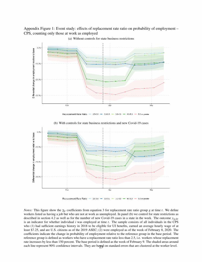
Appendix Figure 1: Event study: effects of replacement rate ratio on probability of employment –CPS, counting only those at work as employed

(a) Without controls for state business restrictions

(b) With controls for state business restrictions and new Covid-19 cases

Notes: This figure show the γgt coefficients from equation 3 for replacement rate ratio group g at time t. We defineworkers listed as having a job but who are not at work as unemployed. In panel (b) we control for state restrictions asdescribed in section 4.2 as well as for the number of new Covid-19 cases in a state in the week. The outcome yig jktis an indicator for whether individual i was employed at time t. The sample consists of all individuals in the CPSwho (1) had sufficient earnings history in 2018 to be eligible for UI benefits, earned an average hourly wage of atleast $7.25, and are U.S. citizens as of the 2019 ASEC; (2) were employed as of the week of February 8, 2020. Thecoefficients indicate the change in probability of employment relative to the reference group in the base period. Thereference group is defined as workers who have a replacement rate ratio less than 2.5, i.e. workers whose replacementrate increases by less than 150 percent. The base period is defined as the week of February 9. The shaded areas aroundeach line represent 90% confidence intervals. They are based on standard errors that are clustered at the worker level.23

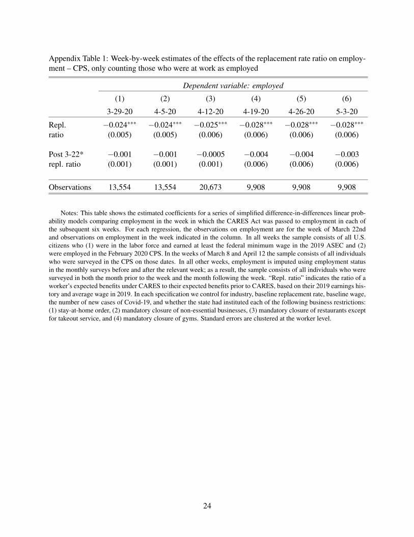
Appendix Table 1: Week-by-week estimates of the effects of the replacement rate ratio on employ-ment – CPS, only counting those who were at work as employed

Dependent variable: employed

(1) (2) (3) (4) (5) (6)

3-29-20 4-5-20 4-12-20 4-19-20 4-26-20 5-3-20

Repl. −0.024∗∗∗ −0.024∗∗∗ −0.025∗∗∗ −0.028∗∗∗ −0.028∗∗∗ −0.028∗∗∗

ratio (0.005) (0.005) (0.006) (0.006) (0.006) (0.006)

Post 3-22* −0.001 −0.001 −0.0005 −0.004 −0.004 −0.003repl. ratio (0.001) (0.001) (0.001) (0.006) (0.006) (0.006)

Observations 13,554 13,554 20,673 9,908 9,908 9,908

Notes: This table shows the estimated coefficients for a series of simplified difference-in-differences linear prob-ability models comparing employment in the week in which the CARES Act was passed to employment in each ofthe subsequent six weeks. For each regression, the observations on employment are for the week of March 22ndand observations on employment in the week indicated in the column. In all weeks the sample consists of all U.S.citizens who (1) were in the labor force and earned at least the federal minimum wage in the 2019 ASEC and (2)were employed in the February 2020 CPS. In the weeks of March 8 and April 12 the sample consists of all individualswho were surveyed in the CPS on those dates. In all other weeks, employment is imputed using employment statusin the monthly surveys before and after the relevant week; as a result, the sample consists of all individuals who weresurveyed in both the month prior to the week and the month following the week. “Repl. ratio” indicates the ratio of aworker’s expected benefits under CARES to their expected benefits prior to CARES, based on their 2019 earnings his-tory and average wage in 2019. In each specification we control for industry, baseline replacement rate, baseline wage,the number of new cases of Covid-19, and whether the state had instituted each of the following business restrictions:(1) stay-at-home order, (2) mandatory closure of non-essential businesses, (3) mandatory closure of restaurants exceptfor takeout service, and (4) mandatory closure of gyms. Standard errors are clustered at the worker level.

24