Embed Size (px)
Citation preview
SAIMAA UNIVERSITY OF APPLIED SCIENCES Technology/Lappeenranta Degree Programme in Mechanical Engineering and Production Technology
Joni Sipponen
EMPLOYING MACHINE VISION TO A MANUFACTURING LINE
Final thesis 2010
ABSTRACT Joni Sipponen Employing machine vision to a manufacturing line, 49 pages, 4 appendices Saimaa University of Applied Sciences, Lappeenranta Technology, Mechanical Engineering and Production Technology Automation and Information Technology Final Thesis 2010 Instructor: Senior lecturer Timo Eloranta, Saimaa University of Applied Sciences The purpose of this thesis was to implement a machine vision system to an assembly line to fix an incorrect placement of a part. If the part is incorrectly positioned, the robot cannot pick it up and the assembly line will come to a stop. The machine vision is connected to a programmable logic controller and the robot. This system is configured to work seamlessly as part of the assembly line. Machine vision will detect if the part is not correctly placed and a flow of air will push the part to the correct position. This thesis was done for the Saimaa University of Applied Sciences. Part of the thesis was to make simple instructions for students, so they are able to quickly learn how to configure the machine vision. The thesis was structured into studying the background of the problem, presenting methods for solving the problem, selecting the method, configuring machine vision, programming the system, and creating the system for fixing the position. Keywords: Machine vision, automation, programmable logic controller

TIIVISTELMÄ Joni Sipponen Konenäön käyttöönotto tuotantolinjalle, 49 sivua, 4 liitettä Saimaan ammattikorkeakoulu, Lappeenranta Tekniikka, Mechanical Engineering and Production Technology Automation and Information Technology Ohjaaja: Lehtori Timo Eloranta, Saimaan ammattikorkeakoulu Lopputyön tavoite oli käyttää konenäköä korjaamaan kokoonpanolinjalla esiintyvä ongelma, jossa osa on väärässä asennossa. Jos osa ei ole kunnolla paikallaan, robotti ei voi nostaa sitä ja kokoonpanolinjan tuotanto pysähtyy. Konenäkö liitettiin ohjelmoitavaan logiikkaan sekä robottiin ja järjestelmä konfiguroitiin toimimaan saumattomasti osana kokoonpanolinjaa. Konenäkö havaitsee jos osa on väärässä asennossa ja ilmasuihku työntää sen paikoilleen. Tämä opinnäytetyö tehtiin Saimaan ammattikorkeakoululle. Osa työtä oli tehdä opiskelijoille yksinkertaiset ohjeet, joista he voivat nopeasti oppia kuinka konfiguroida tämä konenäköjärjestelmä. Opinnäytetyö on rakenteellisesti jaoteltu seuraaviin aiheisiin: ongelman taustatutkimus, ratkaisuvaihtoehdot, vaihtoehdon valinta, konenäön konfigurointi, järjestelmän ohjelmointi ja asennonkorjausjärjestelmän luonti. Asiasanat: Konenäkö, automaatio, ohjelmoitava logiikka
CONTENTS
1 INTRODUCTION ............................................................................................. 6
1.1 Description of the work .............................................................................. 6
1.2 The objective ............................................................................................. 7
2 MANUFACTURING LINE AND MACHINE VISION ......................................... 8
2.1 Manufacturing line ..................................................................................... 8
2.2 Machine vision ........................................................................................... 9
2.2.1 Comparing machine vision and human vision ..................................... 9
2.2.2 CCD-sensor ...................................................................................... 12
2.2.3 Controlling lighting ............................................................................ 13
2.3 F150 Machine vision ................................................................................ 14
3 CAUSE OF THE PROBLEM AND HOW TO PREVENT IT ............................ 15
3.1 Analyzing the failure situation .................................................................. 15
3.2 Reducing loss in momentum ................................................................... 16
3.3 Helping the part to reach the holder......................................................... 17
3.4 Reducing the friction ................................................................................ 18
3.4.1 Friction coefficients ........................................................................... 18
3.4.2 Air resistance .................................................................................... 21
3.4.3 The force needed to reach the holder ............................................... 22
3.4.4 The required reduction of friction ...................................................... 23
4. FIXING INCORRECT POSITION .................................................................. 25
4.1 Dumb system ........................................................................................... 25
4.2 Smart system ........................................................................................... 25
4.3 Comparison of methods ........................................................................... 26
5 IMPLEMENTING MACHINE VISION ............................................................. 28
5.1 Equipment placement .............................................................................. 28
5.1.1 Equipment list ................................................................................... 29
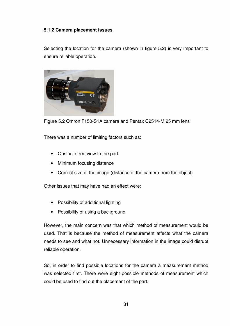
5.1.2 Camera placement issues ................................................................ 31
5.1.3 Equipment locations ......................................................................... 33
5.2 Configuring the machine vision measurement ......................................... 35
5.3 Position correction system ....................................................................... 36
5.4 Wiring of the devices ............................................................................... 38
5.5 Programming of the PLC and the robot ................................................... 39
5.5.1 PLC program .................................................................................... 40
5.5.2 Modifications to the robot program ................................................... 45
6 CONCLUSION ............................................................................................... 45

FIGURES .......................................................................................................... 48
TABLES ............................................................................................................ 48
REFERENCES ................................................................................................. 49
APPENDICES Appendix 1 Test slide measurement results Appendix 2 Symbol table of the PLC program Appendix 3 Mind map for structuring the work Appendix 4 Quick start instructions on configuring F150-3 Vision Sensor
6
1 INTRODUCTION
This thesis concentrates on implementing an automatic visual inspection
system to a production line. Machine vision is technology which belongs to
factory automation, it is a system that takes pictures and interprets them to find
defects or categorize products.
Machine vision systems started to be used widely in the 1980s but the systems
were expensive and required a deep knowledge in computer programming. The
use of machine vision has increased and continues to increase in the industry
due to development of smart cameras which do not need a computer. They
possess all the necessary equipment for machine vision system. These smart
cameras are small, durable and easy to configure by production engineers
(Connolly 2003).
1.1 Description of the work
The purpose of this final thesis is to implement a machine vision system to a
production line to fix a possible problem situation. The production line consists
of Festo’s educational MPS (Modular Production System) equipment which is
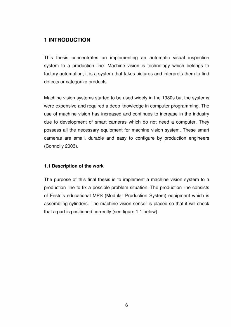
assembling cylinders. The machine vision sensor is placed so that it will check
that a part is positioned correctly (see figure 1.1 below).
7
Figure 1.1 Festo MPS assembly line and a correctly positioned part
If the part is incorrectly positioned the assembly line cannot continue working
and will come to a halt. Part of the thesis is to create a mechanism which fixes
the incorrect position so the assembly line can continue working.
1.2 The objective
The objectives of the final thesis are to study and understand the background of
the problem, find out possible solutions and implement a machine vision system
to solve the problem. The most important part of the thesis is to study and
implement a machine vision system, and to find a way to correct the position of
the part. Implementing the machine vision consists of planning the placement of
the equipment, configuring the machine vision, connecting the machine vision to
work together with a programmable logic controller (PLC) and creating a system
that fixes incorrect position. Also part of the thesis is to create instructions for
automation students on how to configure the machine vision system.
8
2 MANUFACTURING LINE AND MACHINE VISION
This chapter introduces the manufacturing line equipment related to the thesis,
following an explanation of the basic working principles of machine vision and
description of the smart camera which is to be implemented.
2.1 Manufacturing line
For understanding the problem, it is relevant to know how the manufacturing
line equipment works adjacent to the problem. The working area and equipment
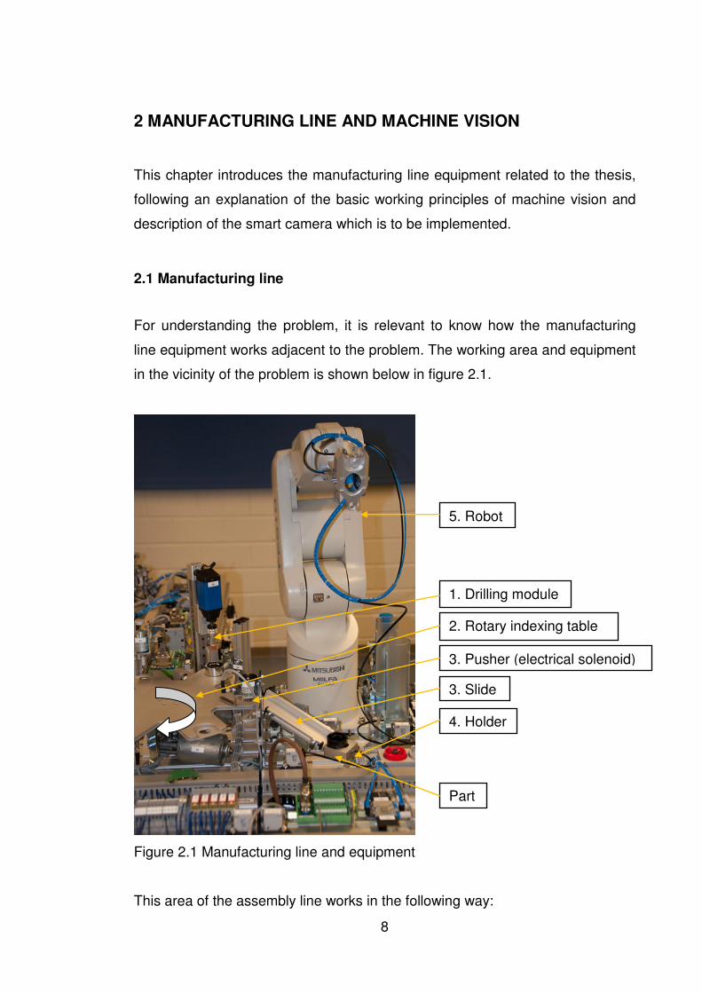
in the vicinity of the problem is shown below in figure 2.1.
Figure 2.1 Manufacturing line and equipment
This area of the assembly line works in the following way:
Part
5. Robot
3. Pusher (electrical solenoid)
3. Slide
1. Drilling module
4. Holder
2. Rotary indexing table
9
1. The part is drilled in the drilling module.
2. The rotary indexing table rotates the part next to the pusher.
3. The pusher pushes the part down the slide.
4. The part reaches the holder.
5. The robot picks up the part. The cycle starts again.
Problem situation occurs when a part does not reach the holder completely but
stays partly on the slider. When the part is not in correct position the robot will
fail to pick up the part.
2.2 Machine vision
When talking about machine vision it means a computer vision system that is
used to replace a worker by taking pictures and processing them. The basic
working principle of machine vision is that a camera takes a picture, and sends
it to a computer. The computer will accept or reject the status according to the
rules programmed in it. That decision will be sent to another device which will
then function according to that information. Smart cameras are machine vision
systems that do not need an external computer but have a controller which acts
as the computer.
Black and white machine vision systems have replaced humans in many areas
but color machine vision has a reputation for being expensive and difficult to
use. This assumption is based on experience with older systems. (Soloman,
p.543.)
There is a wide variety of applications ranging from manufacturing line product
inspection, to helping AGVs (Automated Guided Vehicles) to find their way in a
warehouse (Sarviluoma 2009).
2.2.1 Comparing machine vision and human vision
In this chapter the term human vision is used to indicate human performing an
inspection. It is easy to understand machine vision by comparing machine
10
vision system to a worker. Many parts of the machine vision system are
analogous to human vision.
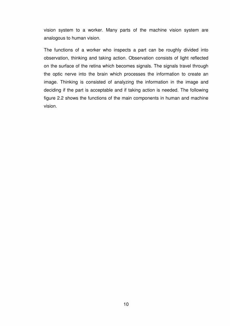
The functions of a worker who inspects a part can be roughly divided into
observation, thinking and taking action. Observation consists of light reflected
on the surface of the retina which becomes signals. The signals travel through
the optic nerve into the brain which processes the information to create an
image. Thinking is consisted of analyzing the information in the image and
deciding if the part is acceptable and if taking action is needed. The following
figure 2.2 shows the functions of the main components in human and machine
vision.
11
Figure 2.2 Function of machine and human vision
The arrow in the middle of the figure shows the flow of information which is
affecting the output, based on programmed rules on the vision system. The
difference in camera and human eye is that camera takes a picture, while
human eye is constantly monitoring the image like a video camera.
When comparing human vision with machine vision on a “solution to a problem”
basis they are very different. The image processing capabilities of the brain are
greatly superior to any machine vision controller/computer software. The brain
12
can adjust well to under/over lighted images and constant adjusting of the
image quality ensures function in changing environments. (Hornberg 2006,
pp.29 - 31.)
To ensure reliable operation for machine vision, the lighting conditions must
usually be highly controlled. Machine vision is better in that the camera does not
get tired, distracted, bored or sick, and in a controlled environment machine
vision is cheaper, less risky and more reliable. Using machine vision it is
possible to calculate distances and areas, gain accurate numerical values and it
enables high speed examination of defects that may be difficult for a worker to
notice.
2.2.2 CCD-sensor
Machine vision system cannot function without a clear image, so it is very
important to guarantee a steady environment for the camera to work. The
previous chapter explained the overview of machine vision components and this
chapter explains how a camera works to be able to understand issues that
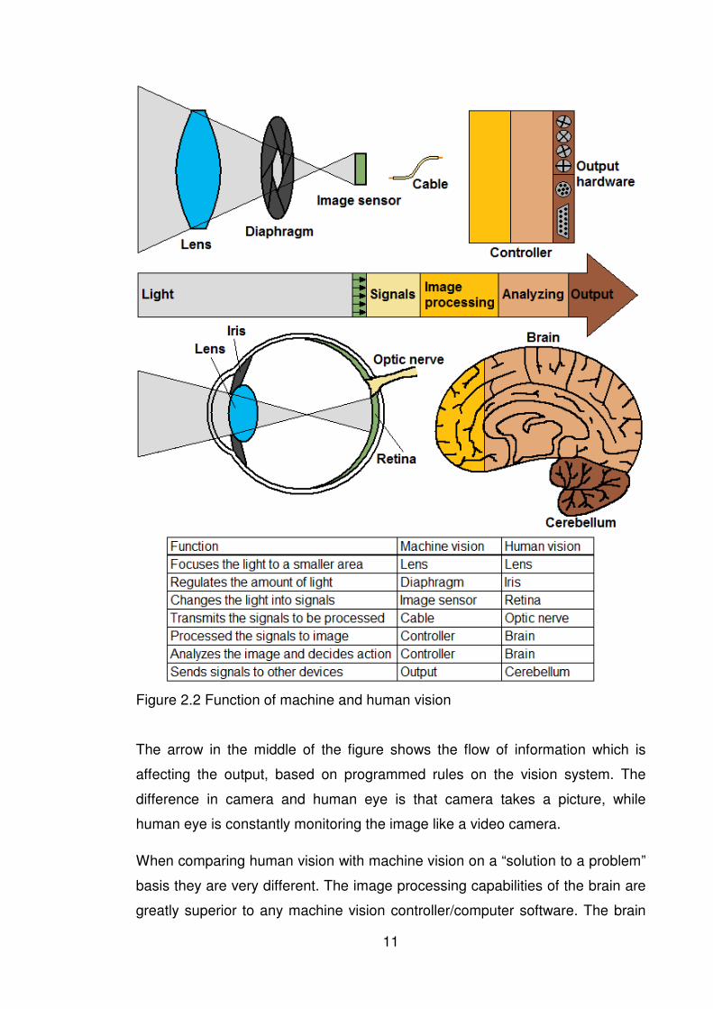
affect image quality. Digital cameras have an image sensor which is responsible
for capturing the image, equivalent to a film on a traditional camera. The most
used image sensor type in digital cameras is CCD (charge-coupled device)
sensor (figure 2.3).
Figure 2.3 CCD sensor and shutter inside a camera
13
CCD sensor consists of cells and each cell obtains an electric charge
proportional to the intensity of light projected on to it. The charges are converted
into voltages which are used to form a black and white image. (Ochi et al.
1997.)
A shutter is a device inside the camera which opens for a period of time to let
light pass into the image sensor. The time the shutter remains open, allowing
more light to pass onto the sensor, is called shutter speed. In lower light
conditions the shutter needs to stay open longer and if the object or the camera
is moving, it can blur the image. A bigger aperture, which is adjusted by the
diaphragm (see figure 2.2), allows more light to reach the sensor in shorter time
but causes loss in depth of field (the area of a picture that is sharp).
2.2.3 Controlling lighting
Depending on the application the need for lighting is very different. Lighting is
used to help the camera get accurate information about issues important for the
examining.
When examining the shape or position of an object, often back lighting is used
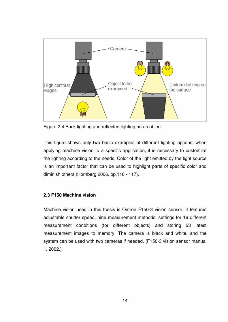
to highlight the edges for easy recognition (figure 2.4). Reflected lighting is used
when performing surface inspections, to gain uniform light distribution on the
surface of the object. (F150-3 vision sensor manual 1, 2002, pp.23-24.)
14
Figure 2.4 Back lighting and reflected lighting on an object
This figure shows only two basic examples of different lighting options, when
applying machine vision to a specific application, it is necessary to customize
the lighting according to the needs. Color of the light emitted by the light source
is an important factor that can be used to highlight parts of specific color and
diminish others (Hornberg 2006, pp.116 - 117).
2.3 F150 Machine vision
Machine vision used in this thesis is Omron F150-3 vision sensor. It features
adjustable shutter speed, nine measurement methods, settings for 16 different
measurement conditions (for different objects) and storing 23 latest
measurement images to memory. The camera is black and white, and the
system can be used with two cameras if needed. (F150-3 vision sensor manual
1, 2002.)
15
3 CAUSE OF THE PROBLEM AND HOW TO PREVENT IT
This chapter describes how the failure occurs and what mechanical reasons are
behind it. It also illustrates possible methods for preventing the problem.
3.1 Analyzing the failure situation
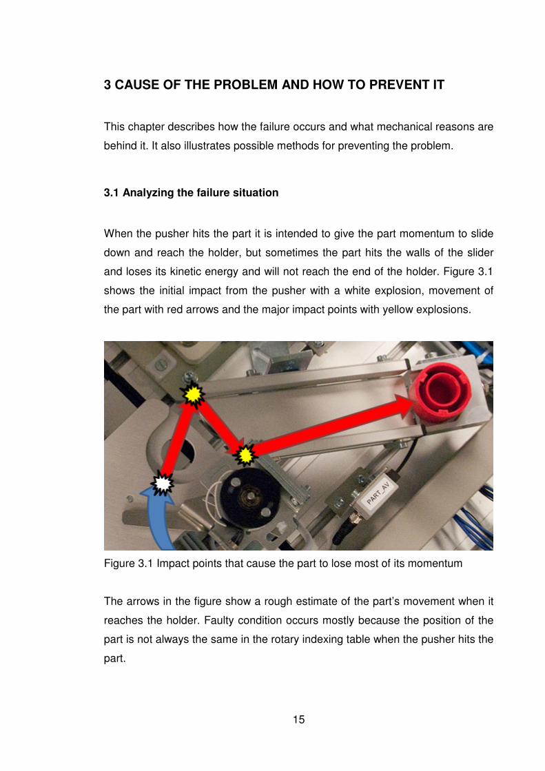
When the pusher hits the part it is intended to give the part momentum to slide
down and reach the holder, but sometimes the part hits the walls of the slider
and loses its kinetic energy and will not reach the end of the holder. Figure 3.1
shows the initial impact from the pusher with a white explosion, movement of
the part with red arrows and the major impact points with yellow explosions.
Figure 3.1 Impact points that cause the part to lose most of its momentum
The arrows in the figure show a rough estimate of the part’s movement when it
reaches the holder. Faulty condition occurs mostly because the position of the
part is not always the same in the rotary indexing table when the pusher hits the
part.
16
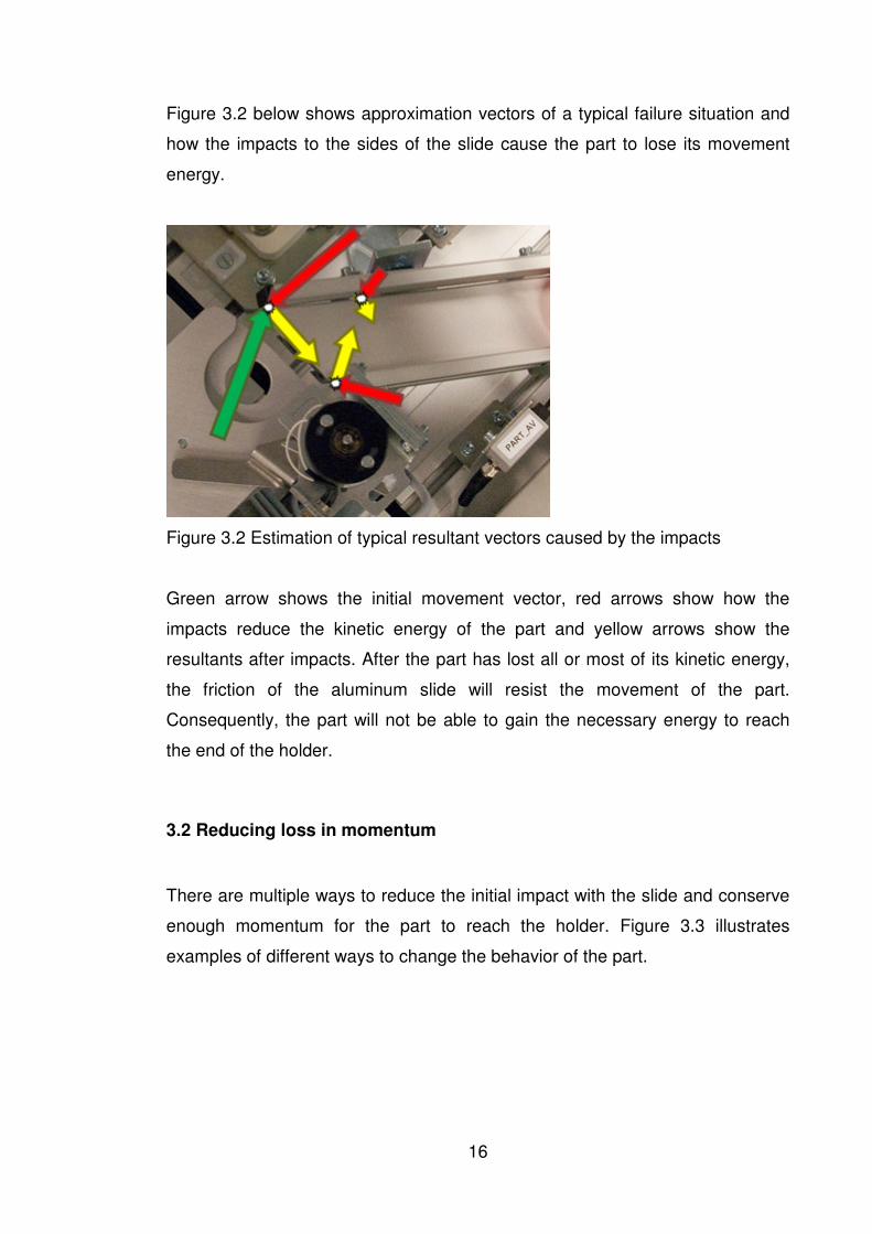
Figure 3.2 below shows approximation vectors of a typical failure situation and
how the impacts to the sides of the slide cause the part to lose its movement
energy.
Figure 3.2 Estimation of typical resultant vectors caused by the impacts
Green arrow shows the initial movement vector, red arrows show how the
impacts reduce the kinetic energy of the part and yellow arrows show the
resultants after impacts. After the part has lost all or most of its kinetic energy,
the friction of the aluminum slide will resist the movement of the part.
Consequently, the part will not be able to gain the necessary energy to reach
the end of the holder.
3.2 Reducing loss in momentum
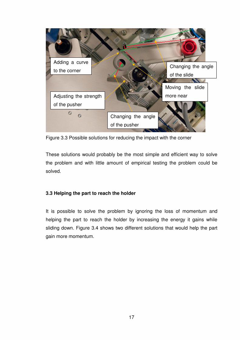
There are multiple ways to reduce the initial impact with the slide and conserve
enough momentum for the part to reach the holder. Figure 3.3 illustrates
examples of different ways to change the behavior of the part.
17
Figure 3.3 Possible solutions for reducing the impact with the corner
These solutions would probably be the most simple and efficient way to solve
the problem and with little amount of empirical testing the problem could be
solved.
3.3 Helping the part to reach the holder
It is possible to solve the problem by ignoring the loss of momentum and
helping the part to reach the holder by increasing the energy it gains while
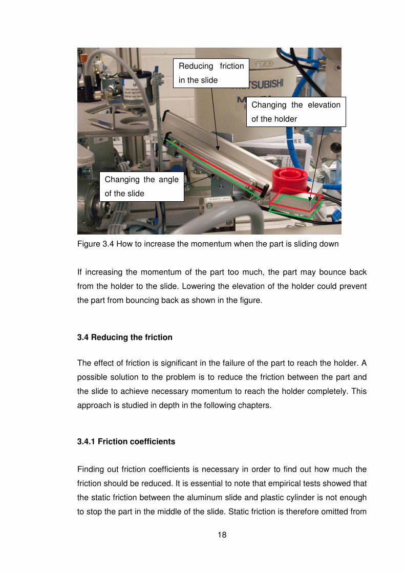
sliding down. Figure 3.4 shows two different solutions that would help the part
gain more momentum.
Changing the angle
of the pusher
Changing the angle
of the slide
Adding a curve
to the corner
Moving the slide
more near Adjusting the strength
of the pusher
18
Figure 3.4 How to increase the momentum when the part is sliding down
If increasing the momentum of the part too much, the part may bounce back
from the holder to the slide. Lowering the elevation of the holder could prevent
the part from bouncing back as shown in the figure.
3.4 Reducing the friction
The effect of friction is significant in the failure of the part to reach the holder. A
possible solution to the problem is to reduce the friction between the part and
the slide to achieve necessary momentum to reach the holder completely. This
approach is studied in depth in the following chapters.
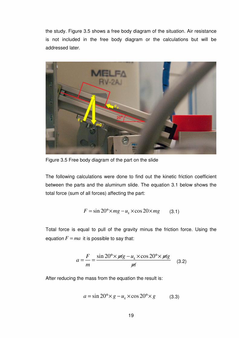
3.4.1 Friction coefficients
Finding out friction coefficients is necessary in order to find out how much the
friction should be reduced. It is essential to note that empirical tests showed that
the static friction between the aluminum slide and plastic cylinder is not enough
to stop the part in the middle of the slide. Static friction is therefore omitted from
Changing the angle
of the slide
Changing the elevation
of the holder
Reducing friction
in the slide
19
the study. Figure 3.5 shows a free body diagram of the situation. Air resistance
is not included in the free body diagram or the calculations but will be
addressed later.
Figure 3.5 Free body diagram of the part on the slide
The following calculations were done to find out the kinetic friction coefficient
between the parts and the aluminum slide. The equation 3.1 below shows the
total force (sum of all forces) affecting the part:
sin 20 cos 20kF mg u mg= °× − × × (3.1)
Total force is equal to pull of the gravity minus the friction force. Using the
equation F ma= it is possible to say that:
sin 20 cos 20k
mg u mgFa
m m
°× − × °×= = (3.2)
After reducing the mass from the equation the result is:
sin 20 cos 20ka g u g= °× − × °× (3.3)
20
It is possible to add the previous equation (3.3) to the following:
2
0 0
1
2x x v t at= + + (3.4)
As the initial position 0x and velocity 0
v are zero the equation will be:
21(sin 20 cos 20 )
2k
x g u g t= °× − × °× (3.5)
Solving the kinetic friction will change the equation into the following form:
22 sin 20
cos 20k
xg
tu
g
− °×
= −
°× (3.6)
It is now possible to calculate the estimated kinetic friction coefficient using this
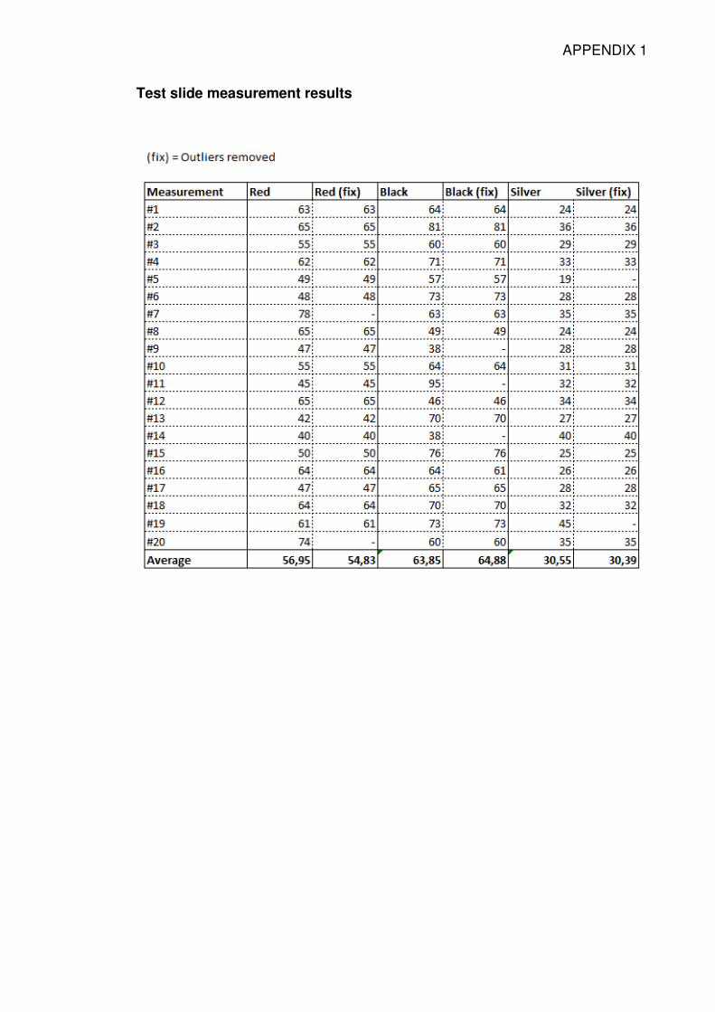
equation. To find out the time a total of 20 test slides were done for each three
different plastic parts. After removing the outliers from the results (See appendix
1) the average times were calculated. When knowing the time and distance the
coefficients were calculated. The resulting kinetic friction coefficients of the
parts are listed in the table 3.1
Table 3.1 Kinetic friction coefficients of the parts
The paint on the red and black parts seem to have about the same kinetic
friction coefficient with the aluminum slide, but the silver colored part has
definitely a lower coefficient and the difference in time is significant. It must be
taken into account that these are rough estimates which are heavily influenced
21
by unstable measuring circumstances, dropping the part by hand to the slide
and measuring the time manually. The calculations also do not take into
account the air resistance which may have an effect on the lightweight plastic
cylinder bottom and thus affect the estimated coefficients.
3.4.2 Air resistance
The air resistance is necessary to evaluate, because of the possible effect it has
on the calculation of the friction coefficient. The force of the air resistance
encountered by the parts is calculated using drag equation:
21
2d w
F c A vρ= × (3.7)
Figure 3.6 illustrates the behavior of the air flow on the part.
Figure 3.6 Air flow around the part when it is sliding in a 20 degree slope
This figure shows that when the part is sliding down in an angle, part of the air
resisting the movement travels inside the cavities of the cylinder bottom, while
other part of the air circles the cylinder smoothly. These are the reasons why
drag coefficient wc is estimated to be 0.9.
22
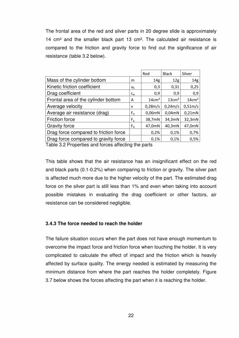
The frontal area of the red and silver parts in 20 degree slide is approximately
14 cm² and the smaller black part 13 cm². The calculated air resistance is
compared to the friction and gravity force to find out the significance of air
resistance (table 3.2 below).
Red Black Silver
Mass of the cylinder bottom m 14g 12g 14g
Kinetic friction coefficient uk 0,3 0,31 0,25
Drag coefficient cw 0,9 0,9 0,9
Frontal area of the cylinder bottom A 14cm² 13cm² 14cm²
Average velocity v 0,28m/s 0,24m/s 0,51m/s
Average air resistance (drag) Fd 0,06mN 0,04mN 0,21mN
Friction force Fμ 38,7mN 34,3mN 32,3mN
Gravity force FG 47,0mN 40,3mN 47,0mN
Drag force compared to friction force 0,2% 0,1% 0,7%
Drag force compared to gravity force 0,1% 0,1% 0,5%
Table 3.2 Properties and forces affecting the parts
This table shows that the air resistance has an insignificant effect on the red
and black parts (0.1-0.2%) when comparing to friction or gravity. The silver part
is affected much more due to the higher velocity of the part. The estimated drag
force on the silver part is still less than 1% and even when taking into account
possible mistakes in evaluating the drag coefficient or other factors, air
resistance can be considered negligible.
3.4.3 The force needed to reach the holder
The failure situation occurs when the part does not have enough momentum to
overcome the impact force and friction force when touching the holder. It is very
complicated to calculate the effect of impact and the friction which is heavily
affected by surface quality. The energy needed is estimated by measuring the
minimum distance from where the part reaches the holder completely. Figure
3.7 below shows the forces affecting the part when it is reaching the holder.
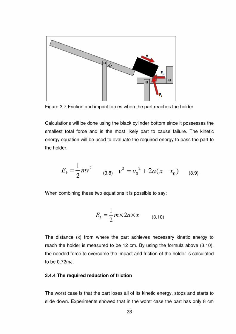
23
Figure 3.7 Friction and impact forces when the part reaches the holder
Calculations will be done using the black cylinder bottom since it possesses the
smallest total force and is the most likely part to cause failure. The kinetic
energy equation will be used to evaluate the required energy to pass the part to
the holder.
21
2k
E mv= (3.8) 2 2
0 02 ( )v v a x x= + − (3.9)
When combining these two equations it is possible to say:
12
2kE m a x= × × (3.10)
The distance (x) from where the part achieves necessary kinetic energy to
reach the holder is measured to be 12 cm. By using the formula above (3.10),
the needed force to overcome the impact and friction of the holder is calculated
to be 0.72mJ.
3.4.4 The required reduction of friction
The worst case is that the part loses all of its kinetic energy, stops and starts to
slide down. Experiments showed that in the worst case the part has only 8 cm
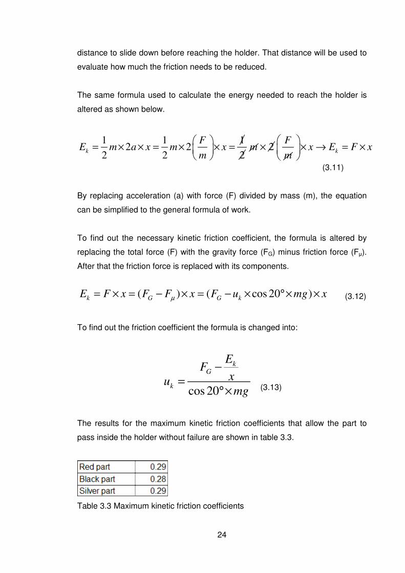
24
distance to slide down before reaching the holder. That distance will be used to
evaluate how much the friction needs to be reduced.
The same formula used to calculate the energy needed to reach the holder is
altered as shown below.
1 1 12 2 2
2 2 2k k
F FE m a x m x m x E F x
m m
= × × = × × = × × → = ×
(3.11)
By replacing acceleration (a) with force (F) divided by mass (m), the equation
can be simplified to the general formula of work.
To find out the necessary kinetic friction coefficient, the formula is altered by
replacing the total force (F) with the gravity force (FG) minus friction force (Fµ).
After that the friction force is replaced with its components.
( ) ( cos 20 )k G G k
E F x F F x F u mg xµ= × = − × = − × °× × (3.12)
To find out the friction coefficient the formula is changed into:
cos 20
kG
k
EF
xumg
−
=°× (3.13)
The results for the maximum kinetic friction coefficients that allow the part to
pass inside the holder without failure are shown in table 3.3.
Table 3.3 Maximum kinetic friction coefficients
25
Note that the silver part already has a much lower kinetic friction coefficient (see
table 3.1) and does not experience the problem situation. The black part has a
bit lower value. This is because it has less mass and it needs more velocity to
achieve the same kinetic energy as the other parts. These values represent the
maximum kinetic friction coefficients that allow the part pass in to the holder
reliably. They could be achieved using for example painting the surface of the
slide, using another material than aluminum for the slide, sanding the surface to
be smoother, etc.
4. FIXING INCORRECT POSITION
This chapter does not focus on preventing the problem but instead presents
logic driven solutions for fixing the problem. The chapter presents different logic
systems for fixing the incorrect position and evaluates them. The method used
for mechanically fixing the position is selected later.
4.1 Dumb system
The idea of dumb system is that the logic does not know if the part is correctly
placed or not. The system would try to fix the position always, forcing the part to
reach the holder. The weak point of the system is that it has no way of knowing
if the position was fixed correctly. This could be done using either the robot or a
programmable logic controller.
4.2 Smart system
This system would know when the part is correctly placed by using a sensor.
Only when there is a problem it would attempt to fix the position. After fixing the
position, the system checks the position again and gives a go-signal for the
robot.
26
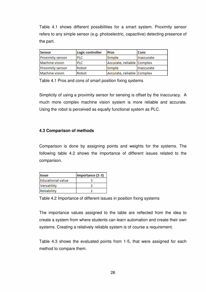
Table 4.1 shows different possibilities for a smart system. Proximity sensor
refers to any simple sensor (e.g. photoelectric, capacitive) detecting presence of
the part.
Table 4.1 Pros and cons of smart position fixing systems
Simplicity of using a proximity sensor for sensing is offset by the inaccuracy. A
much more complex machine vision system is more reliable and accurate.
Using the robot is perceived as equally functional system as PLC.
4.3 Comparison of methods
Comparison is done by assigning points and weights for the systems. The
following table 4.2 shows the importance of different issues related to the
comparison.
Table 4.2 Importance of different issues in position fixing systems
The importance values assigned to the table are reflected from the idea to
create a system from where students can learn automation and create their own
systems. Creating a relatively reliable system is of course a requirement.
Table 4.3 shows the evaluated points from 1-5, that were assigned for each
method to compare them.
27
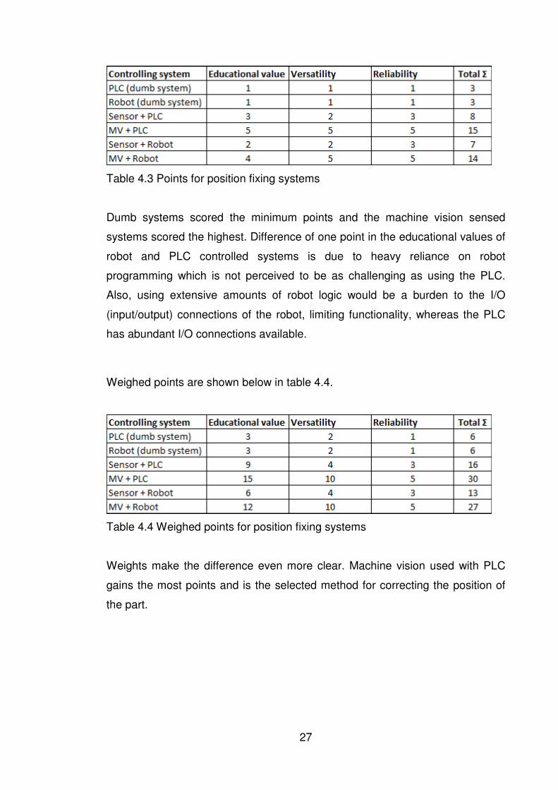
Table 4.3 Points for position fixing systems
Dumb systems scored the minimum points and the machine vision sensed
systems scored the highest. Difference of one point in the educational values of
robot and PLC controlled systems is due to heavy reliance on robot
programming which is not perceived to be as challenging as using the PLC.
Also, using extensive amounts of robot logic would be a burden to the I/O
(input/output) connections of the robot, limiting functionality, whereas the PLC
has abundant I/O connections available.
Weighed points are shown below in table 4.4.
Table 4.4 Weighed points for position fixing systems
Weights make the difference even more clear. Machine vision used with PLC
gains the most points and is the selected method for correcting the position of
the part.
28
5 IMPLEMENTING MACHINE VISION
The main part of this thesis is to create a functioning fault recognition/fixing
system via the aid of machine vision and this chapter will describe the work
done from scratch to a working system. The subchapters will be describing the
following topics:
• 5.1 Equipment placement
• 5.2 Configuring the machine vision
• 5.3 Methods for position correction
• 5.4 Programming of the PLC and the robot
The chapters are not in chronological order, because in reality the work was
done in many levels at the same time and it is much more feasible for the
reader to understand them when presented individually.
5.1 Equipment placement
When choosing the placement for the equipment it was necessary to consider
the following basic prerequisites:
• Ability of the machinery to work as expected
• Rigid attaching
• Environmental disruptions
• Obstacle free access to nearby equipment
• Safety issues for the users
The equipment was placed considering these issues.
The installation environment is very stable as it is a school automation
laboratory. There are no problems arising from temperature, condensation,
29
humidity, dust, vibration, chemicals, gases or other possibly hazardous issues
for the equipment. As the equipment is designed to be used in much worse
environment (factory) the surroundings are very reliable. The only concerns the
environment brings are the other equipment in close proximity, power cables
and users.
5.1.1 Equipment list
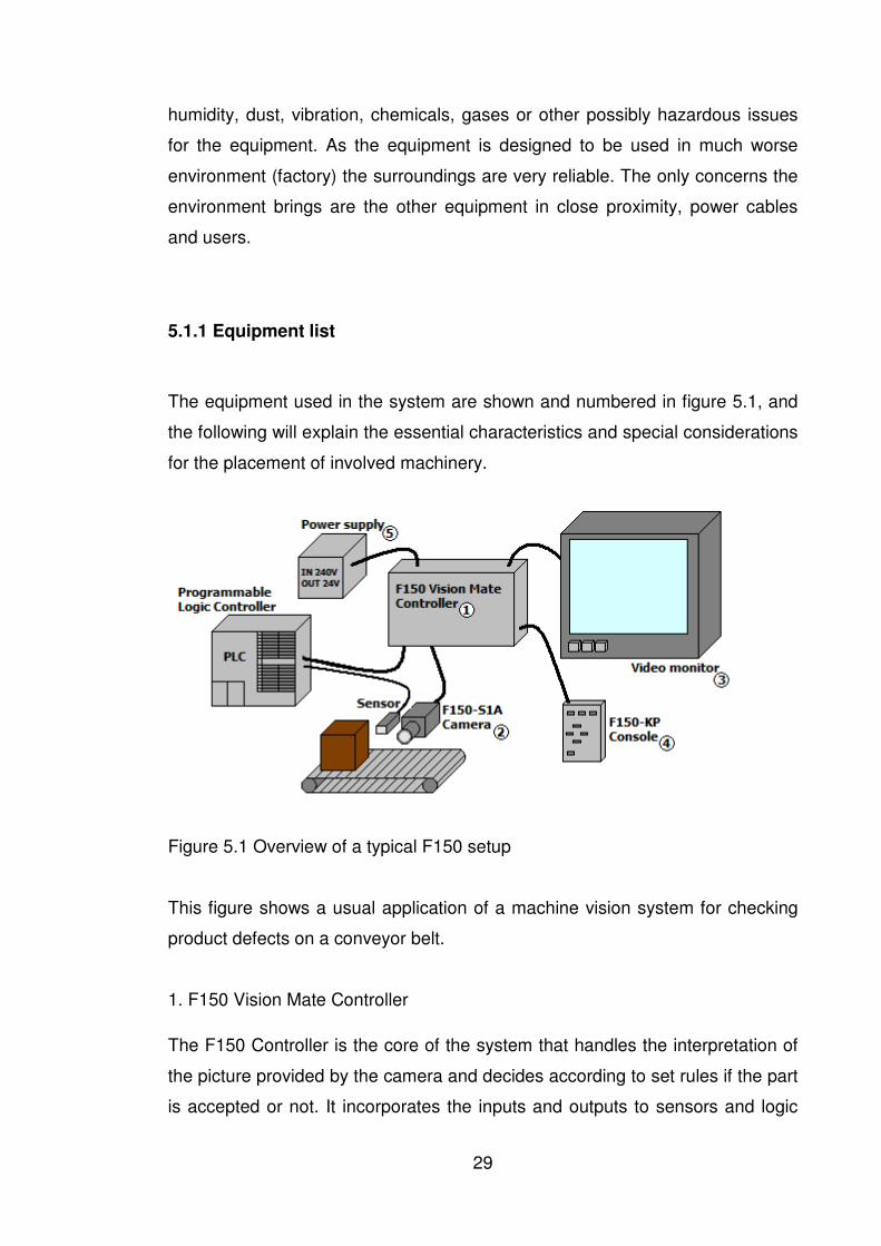
The equipment used in the system are shown and numbered in figure 5.1, and
the following will explain the essential characteristics and special considerations
for the placement of involved machinery.
Figure 5.1 Overview of a typical F150 setup
This figure shows a usual application of a machine vision system for checking
product defects on a conveyor belt.
1. F150 Vision Mate Controller
The F150 Controller is the core of the system that handles the interpretation of
the picture provided by the camera and decides according to set rules if the part
is accepted or not. It incorporates the inputs and outputs to sensors and logic
30
controllers, so it should be located in a place which allows easy connection to
this equipment.
F150 must be installed in a specific orientation and needs to have a minimum
clearance of 50 mm above and below to improve heat dissipation. There should
be 200 mm space between the controller and power cables to avoid electrical
noise. (F150-3 vision sensor manual 1, 2002, pp.2-4.)
2. F150-S1A Camera
The camera is responsible for taking the pictures and sending them to the F150
Controller. Special consideration for the placement of the camera must be done
due to the importance of clear image and gaining the needed information from
the picture. Due to the environment (students) accidental knocks may change
the orientation of the camera. Rigid attaching is important. Camera case is
connected to internal circuit 0V line and should not be grounded to avoid noise
interference (F150-3 vision sensor manual 1, 2002, p.4).
3. Ikegami Video Monitor
The video monitor is to be placed in an accessible place to be able to monitor
the function of the camera and to adjust the settings of the controller.
4. F150-KP Console
The console is used to configure the controller. It should be readily available for
using and have a location where it can be put safely when not in use.
5. S82K-03024 Power supply
Care must be taken in the placement of the power supply as hazardous
voltages are involved (230VAC).
31
5.1.2 Camera placement issues
Selecting the location for the camera (shown in figure 5.2) is very important to
ensure reliable operation.
Figure 5.2 Omron F150-S1A camera and Pentax C2514-M 25 mm lens
There was a number of limiting factors such as:
• Obstacle free view to the part
• Minimum focusing distance
• Correct size of the image (distance of the camera from the object)
Other issues that may have had an effect were:
• Possibility of additional lighting
• Possibility of using a background
However, the main concern was that which method of measurement would be
used. That is because the method of measurement affects what the camera
needs to see and what not. Unnecessary information in the image could disrupt
reliable operation.
So, in order to find possible locations for the camera a measurement method
was selected first. There were eight possible methods of measurement which
could be used to find out the placement of the part.
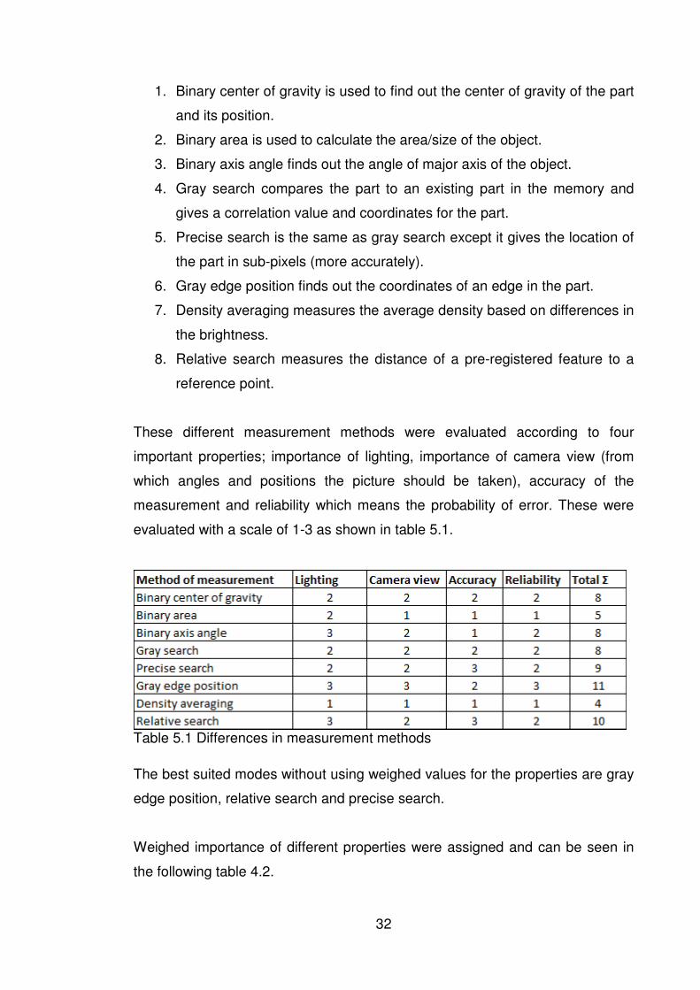
32
1. Binary center of gravity is used to find out the center of gravity of the part
and its position.
2. Binary area is used to calculate the area/size of the object.
3. Binary axis angle finds out the angle of major axis of the object.
4. Gray search compares the part to an existing part in the memory and
gives a correlation value and coordinates for the part.
5. Precise search is the same as gray search except it gives the location of
the part in sub-pixels (more accurately).
6. Gray edge position finds out the coordinates of an edge in the part.
7. Density averaging measures the average density based on differences in
the brightness.
8. Relative search measures the distance of a pre-registered feature to a
reference point.
These different measurement methods were evaluated according to four
important properties; importance of lighting, importance of camera view (from
which angles and positions the picture should be taken), accuracy of the
measurement and reliability which means the probability of error. These were
evaluated with a scale of 1-3 as shown in table 5.1.
Table 5.1 Differences in measurement methods
The best suited modes without using weighed values for the properties are gray
edge position, relative search and precise search.
Weighed importance of different properties were assigned and can be seen in
the following table 4.2.
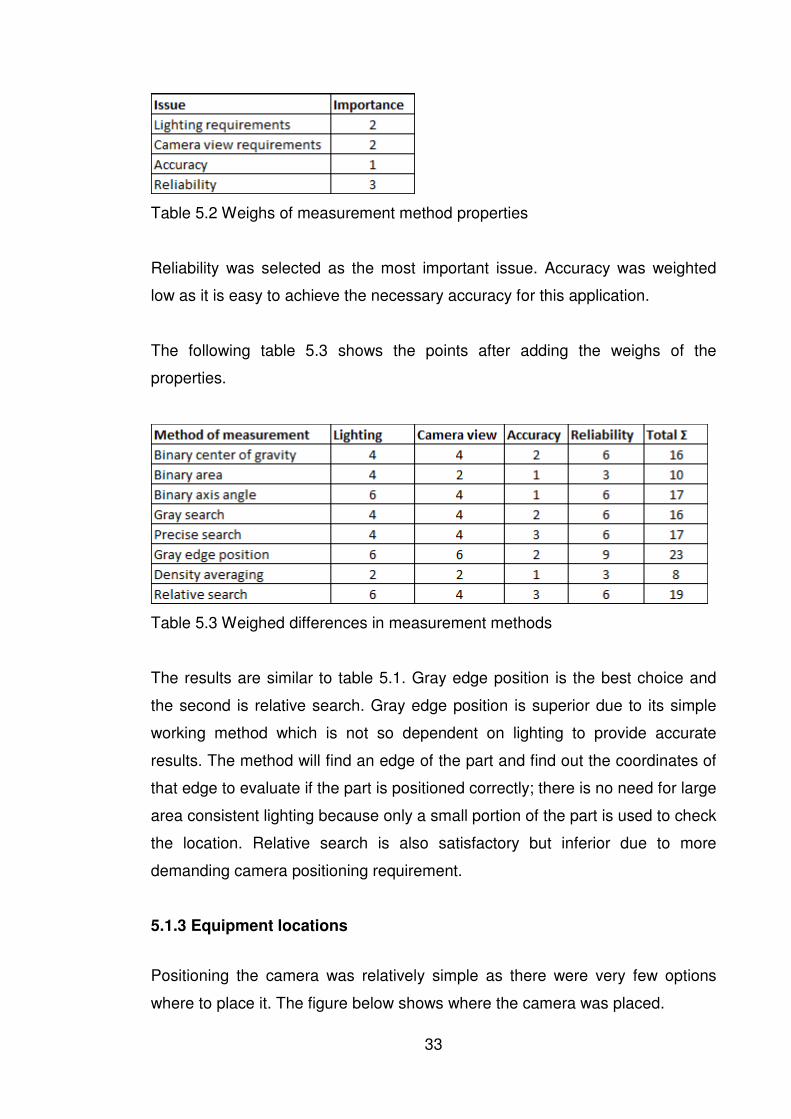
33
Table 5.2 Weighs of measurement method properties
Reliability was selected as the most important issue. Accuracy was weighted
low as it is easy to achieve the necessary accuracy for this application.
The following table 5.3 shows the points after adding the weighs of the
properties.
Table 5.3 Weighed differences in measurement methods
The results are similar to table 5.1. Gray edge position is the best choice and
the second is relative search. Gray edge position is superior due to its simple
working method which is not so dependent on lighting to provide accurate
results. The method will find an edge of the part and find out the coordinates of
that edge to evaluate if the part is positioned correctly; there is no need for large
area consistent lighting because only a small portion of the part is used to check
the location. Relative search is also satisfactory but inferior due to more
demanding camera positioning requirement.
5.1.3 Equipment locations
Positioning the camera was relatively simple as there were very few options
where to place it. The figure below shows where the camera was placed.
34
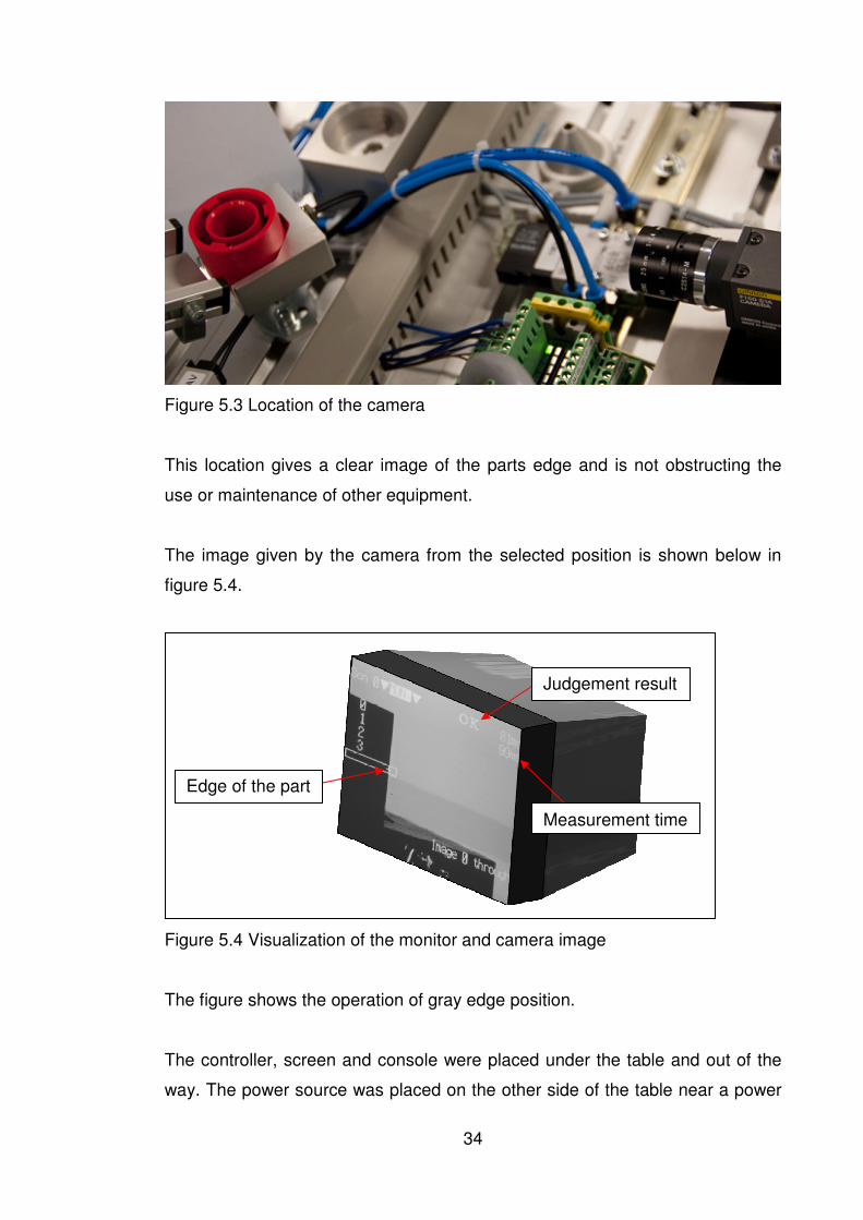
Figure 5.3 Location of the camera
This location gives a clear image of the parts edge and is not obstructing the
use or maintenance of other equipment.
The image given by the camera from the selected position is shown below in
figure 5.4.
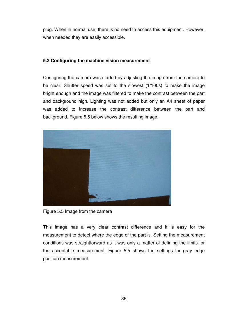
Figure 5.4 Visualization of the monitor and camera image
The figure shows the operation of gray edge position.
The controller, screen and console were placed under the table and out of the
way. The power source was placed on the other side of the table near a power
Edge of the part
Judgement result
Measurement time
35
plug. When in normal use, there is no need to access this equipment. However,
when needed they are easily accessible.
5.2 Configuring the machine vision measurement
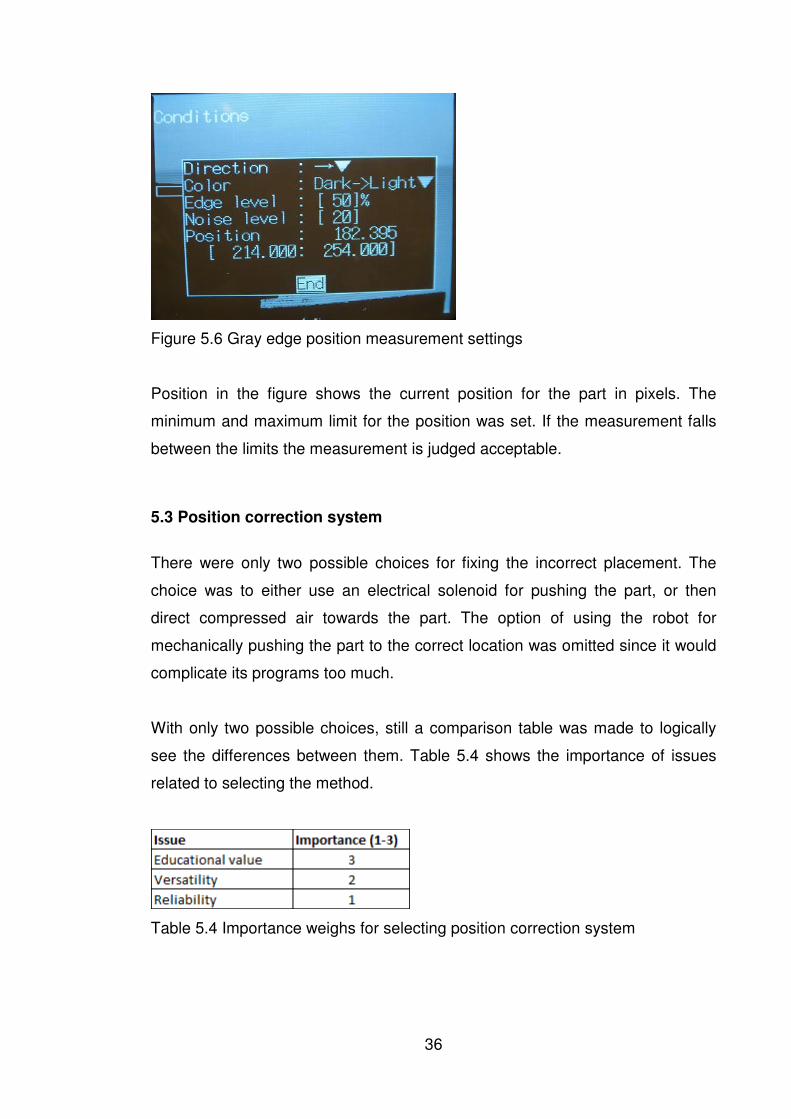
Configuring the camera was started by adjusting the image from the camera to
be clear. Shutter speed was set to the slowest (1/100s) to make the image
bright enough and the image was filtered to make the contrast between the part
and background high. Lighting was not added but only an A4 sheet of paper
was added to increase the contrast difference between the part and
background. Figure 5.5 below shows the resulting image.
Figure 5.5 Image from the camera
This image has a very clear contrast difference and it is easy for the
measurement to detect where the edge of the part is. Setting the measurement
conditions was straightforward as it was only a matter of defining the limits for
the acceptable measurement. Figure 5.5 shows the settings for gray edge
position measurement.
36
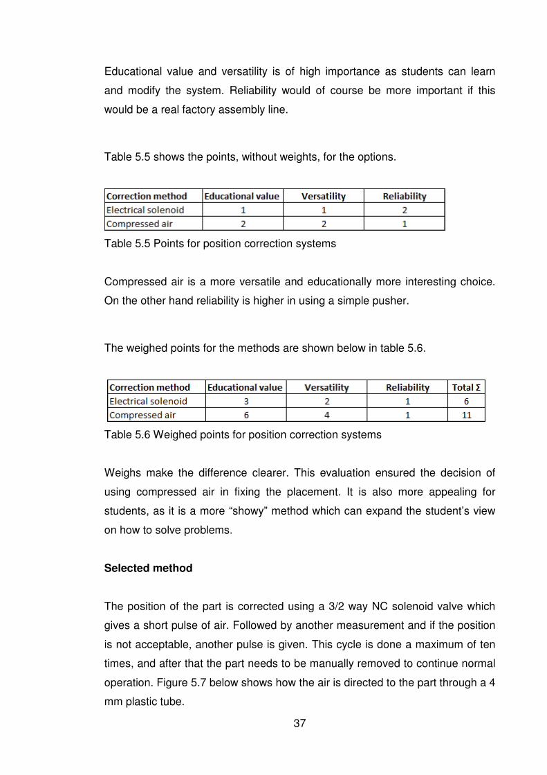
Figure 5.6 Gray edge position measurement settings
Position in the figure shows the current position for the part in pixels. The
minimum and maximum limit for the position was set. If the measurement falls
between the limits the measurement is judged acceptable.
5.3 Position correction system
There were only two possible choices for fixing the incorrect placement. The
choice was to either use an electrical solenoid for pushing the part, or then
direct compressed air towards the part. The option of using the robot for
mechanically pushing the part to the correct location was omitted since it would
complicate its programs too much.
With only two possible choices, still a comparison table was made to logically
see the differences between them. Table 5.4 shows the importance of issues
related to selecting the method.
Table 5.4 Importance weighs for selecting position correction system
37
Educational value and versatility is of high importance as students can learn
and modify the system. Reliability would of course be more important if this
would be a real factory assembly line.
Table 5.5 shows the points, without weights, for the options.
Table 5.5 Points for position correction systems
Compressed air is a more versatile and educationally more interesting choice.
On the other hand reliability is higher in using a simple pusher.
The weighed points for the methods are shown below in table 5.6.
Table 5.6 Weighed points for position correction systems
Weighs make the difference clearer. This evaluation ensured the decision of
using compressed air in fixing the placement. It is also more appealing for
students, as it is a more “showy” method which can expand the student’s view
on how to solve problems.
Selected method
The position of the part is corrected using a 3/2 way NC solenoid valve which
gives a short pulse of air. Followed by another measurement and if the position
is not acceptable, another pulse is given. This cycle is done a maximum of ten
times, and after that the part needs to be manually removed to continue normal
operation. Figure 5.7 below shows how the air is directed to the part through a 4
mm plastic tube.
38
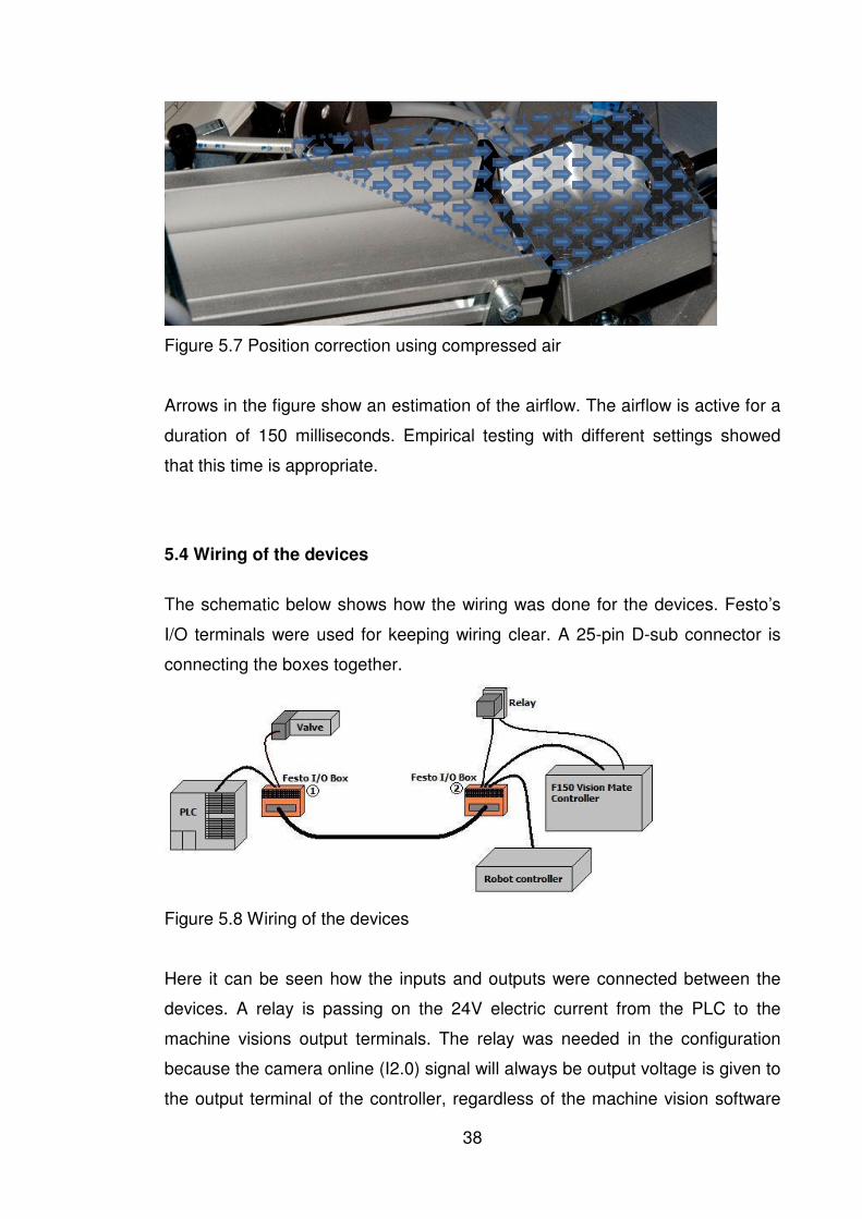
Figure 5.7 Position correction using compressed air
Arrows in the figure show an estimation of the airflow. The airflow is active for a
duration of 150 milliseconds. Empirical testing with different settings showed
that this time is appropriate.
5.4 Wiring of the devices
The schematic below shows how the wiring was done for the devices. Festo’s
I/O terminals were used for keeping wiring clear. A 25-pin D-sub connector is
connecting the boxes together.
Figure 5.8 Wiring of the devices
Here it can be seen how the inputs and outputs were connected between the
devices. A relay is passing on the 24V electric current from the PLC to the
machine visions output terminals. The relay was needed in the configuration
because the camera online (I2.0) signal will always be output voltage is given to
the output terminal of the controller, regardless of the machine vision software
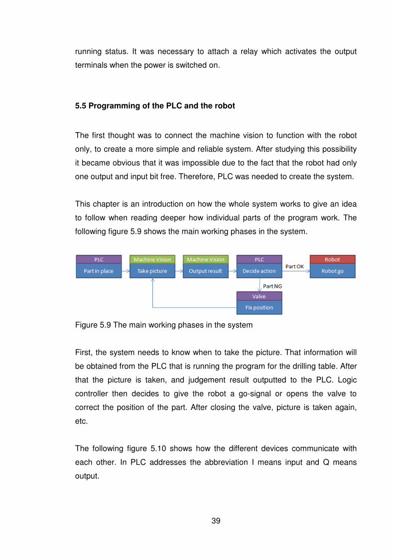
39
running status. It was necessary to attach a relay which activates the output
terminals when the power is switched on.
5.5 Programming of the PLC and the robot
The first thought was to connect the machine vision to function with the robot
only, to create a more simple and reliable system. After studying this possibility
it became obvious that it was impossible due to the fact that the robot had only
one output and input bit free. Therefore, PLC was needed to create the system.
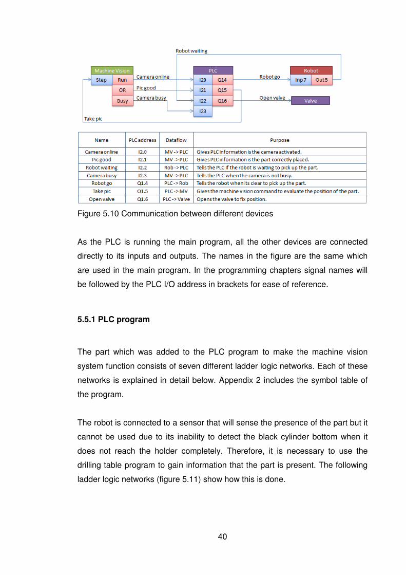
This chapter is an introduction on how the whole system works to give an idea
to follow when reading deeper how individual parts of the program work. The
following figure 5.9 shows the main working phases in the system.
Figure 5.9 The main working phases in the system
First, the system needs to know when to take the picture. That information will
be obtained from the PLC that is running the program for the drilling table. After
that the picture is taken, and judgement result outputted to the PLC. Logic
controller then decides to give the robot a go-signal or opens the valve to
correct the position of the part. After closing the valve, picture is taken again,
etc.
The following figure 5.10 shows how the different devices communicate with
each other. In PLC addresses the abbreviation I means input and Q means
output.
40
Figure 5.10 Communication between different devices
As the PLC is running the main program, all the other devices are connected
directly to its inputs and outputs. The names in the figure are the same which
are used in the main program. In the programming chapters signal names will
be followed by the PLC I/O address in brackets for ease of reference.
5.5.1 PLC program
The part which was added to the PLC program to make the machine vision
system function consists of seven different ladder logic networks. Each of these
networks is explained in detail below. Appendix 2 includes the symbol table of
the program.
The robot is connected to a sensor that will sense the presence of the part but it
cannot be used due to its inability to detect the black cylinder bottom when it
does not reach the holder completely. Therefore, it is necessary to use the
drilling table program to gain information that the part is present. The following
ladder logic networks (figure 5.11) show how this is done.
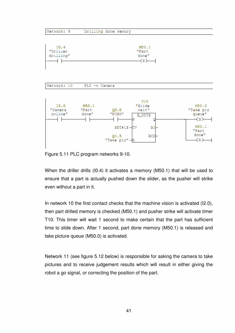
41
Figure 5.11 PLC program networks 9-10.
When the driller drills (I0.4) it activates a memory (M50.1) that will be used to
ensure that a part is actually pushed down the slider, as the pusher will strike
even without a part in it.
In network 10 the first contact checks that the machine vision is activated (I2.0),
then part drilled memory is checked (M50.1) and pusher strike will activate timer
T10. This timer will wait 1 second to make certain that the part has sufficient
time to slide down. After 1 second, part done memory (M50.1) is released and
take picture queue (M50.0) is activated.
Network 11 (see figure 5.12 below) is responsible for asking the camera to take
pictures and to receive judgement results which will result in either giving the
robot a go signal, or correcting the position of the part.
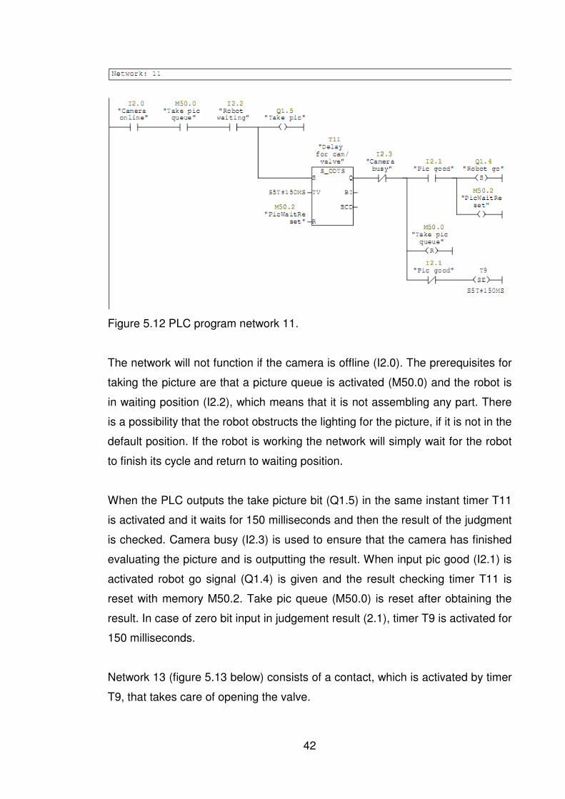
42
Figure 5.12 PLC program network 11.
The network will not function if the camera is offline (I2.0). The prerequisites for
taking the picture are that a picture queue is activated (M50.0) and the robot is
in waiting position (I2.2), which means that it is not assembling any part. There
is a possibility that the robot obstructs the lighting for the picture, if it is not in the
default position. If the robot is working the network will simply wait for the robot
to finish its cycle and return to waiting position.
When the PLC outputs the take picture bit (Q1.5) in the same instant timer T11
is activated and it waits for 150 milliseconds and then the result of the judgment
is checked. Camera busy (I2.3) is used to ensure that the camera has finished
evaluating the picture and is outputting the result. When input pic good (I2.1) is
activated robot go signal (Q1.4) is given and the result checking timer T11 is
reset with memory M50.2. Take pic queue (M50.0) is reset after obtaining the
result. In case of zero bit input in judgement result (2.1), timer T9 is activated for
150 milliseconds.
Network 13 (figure 5.13 below) consists of a contact, which is activated by timer
T9, that takes care of opening the valve.
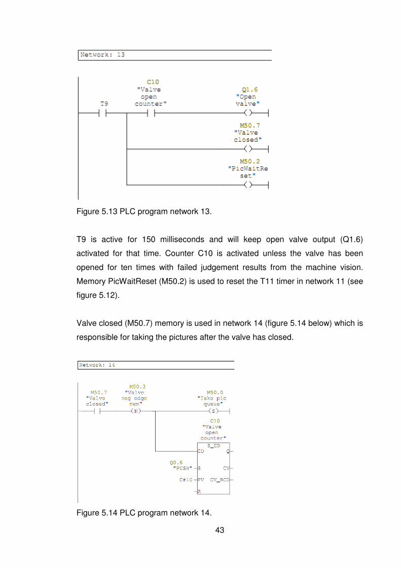
43
Figure 5.13 PLC program network 13.
T9 is active for 150 milliseconds and will keep open valve output (Q1.6)
activated for that time. Counter C10 is activated unless the valve has been
opened for ten times with failed judgement results from the machine vision.
Memory PicWaitReset (M50.2) is used to reset the T11 timer in network 11 (see
figure 5.12).
Valve closed (M50.7) memory is used in network 14 (figure 5.14 below) which is
responsible for taking the pictures after the valve has closed.
Figure 5.14 PLC program network 14.
44
This network also has the timer C10 for counting the number of valve openings.
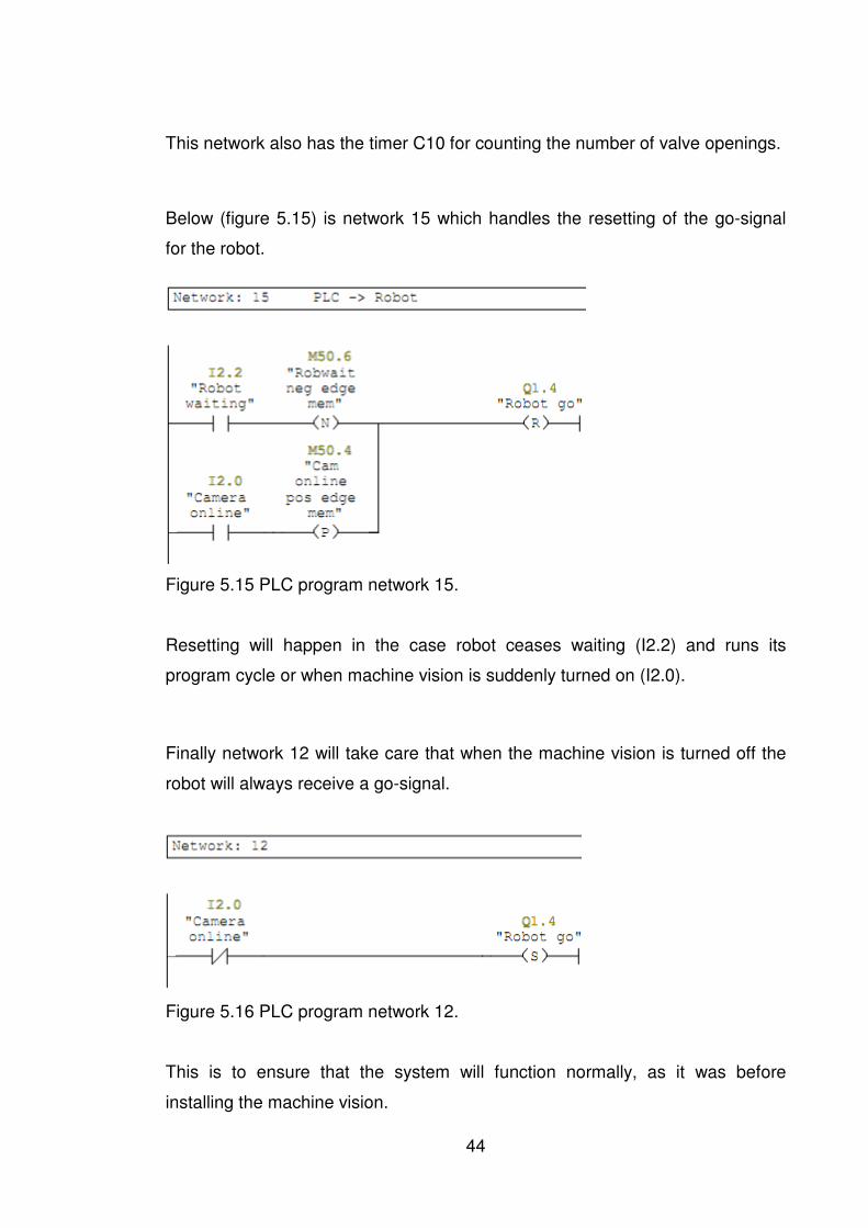
Below (figure 5.15) is network 15 which handles the resetting of the go-signal
for the robot.
Figure 5.15 PLC program network 15.
Resetting will happen in the case robot ceases waiting (I2.2) and runs its
program cycle or when machine vision is suddenly turned on (I2.0).
Finally network 12 will take care that when the machine vision is turned off the
robot will always receive a go-signal.
Figure 5.16 PLC program network 12.
This is to ensure that the system will function normally, as it was before
installing the machine vision.
45
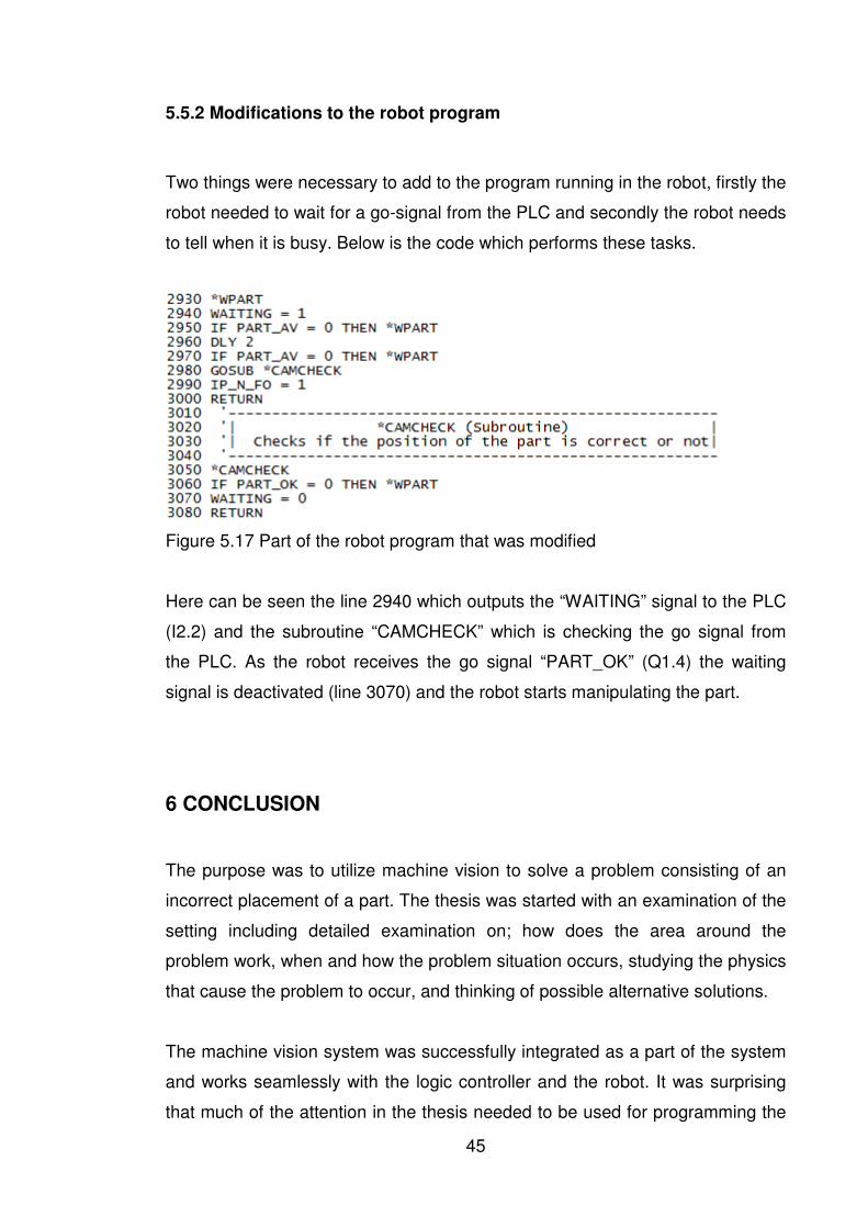
5.5.2 Modifications to the robot program
Two things were necessary to add to the program running in the robot, firstly the
robot needed to wait for a go-signal from the PLC and secondly the robot needs
to tell when it is busy. Below is the code which performs these tasks.
Figure 5.17 Part of the robot program that was modified
Here can be seen the line 2940 which outputs the “WAITING” signal to the PLC
(I2.2) and the subroutine “CAMCHECK” which is checking the go signal from
the PLC. As the robot receives the go signal “PART_OK” (Q1.4) the waiting
signal is deactivated (line 3070) and the robot starts manipulating the part.
6 CONCLUSION
The purpose was to utilize machine vision to solve a problem consisting of an
incorrect placement of a part. The thesis was started with an examination of the
setting including detailed examination on; how does the area around the
problem work, when and how the problem situation occurs, studying the physics
that cause the problem to occur, and thinking of possible alternative solutions.
The machine vision system was successfully integrated as a part of the system
and works seamlessly with the logic controller and the robot. It was surprising
that much of the attention in the thesis needed to be used for programming the
46
logic controller and robot. Configuring machine vision was easy. As expected, a
significant amount of time was used for finding the correct I/O connections
between devices, especially the robot. This thesis supports well the view
described in the introduction chapter by Connolly (2003) which states that smart
cameras are easy to configure.
After the work was finished an instruction manual on how to configure the
machine vision for automation students was made (see appendix 4). It explains
in a simple way how to use the machine vision, so that students may quickly
understand the steps required for configuring.
The work successfully met its goals; the incorrect positioning is detected,
placement fixed, and the robot continues working without interruptions.
Evaluating the consistent functioning was sufficiently checked, but the work
failed in rigid connection of the camera. Only two months later when I came to
check if the system works, somebody had already knocked the camera and the
picture was offset so it would not function as it was intended. The work
remained unfinished with relation to selecting a more permanent background for
the camera image and remains to be used with a blank paper sheet as
background.
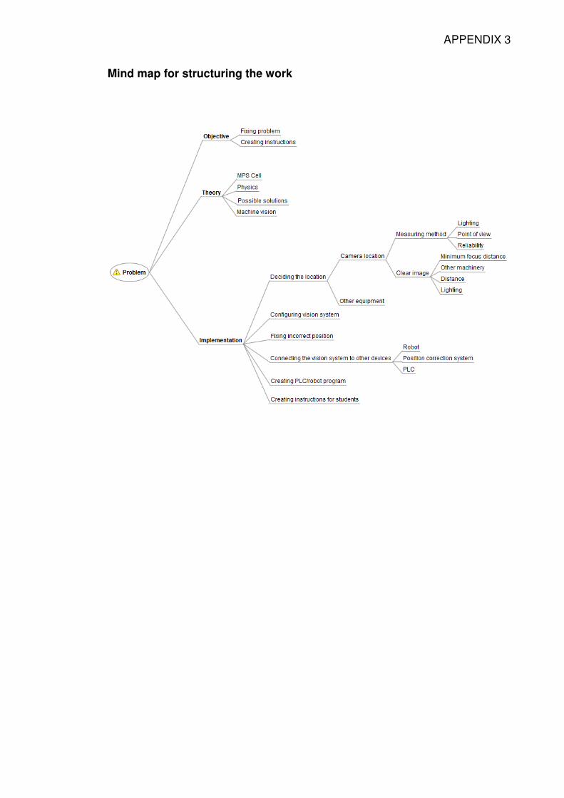
The work done in the final thesis was interesting as it gave the opportunity to
truly work independently and apply knowledge of automation gained through
courses. In the start of the work I created a mind map using FreeMind software
(see appendix 3) and it helped a lot in structuring and understanding different
parts of the work.
The biggest issue while working with the thesis was time management. While
doing courses the thesis got much less attention. What mostly disappointed me
was the configuration of the machine vision measurements, as it was too easy. I
was hoping that it would be more challenging. Working with the robot and PLC
was exciting as the working sequence was relatively unorthodox and
demanding.
47
Problems that I encountered during the work taught me a great deal. Machine
vision as a theme was fascinating and it gave me a lot of very valuable
information. In my opinion the problem solved in the thesis was very simple
compared to what could be done using machine vision. When used correctly
machine vision can be very productive and save many working hours in many
applications.
Future prospects
It would be possible to extend the use of the machine vision within this
assembly line. The following lists some views that could be done.
Mount the machine vision on the robot to create a mobile camera. With this
system it would be possible to check if the part is correctly placed and also to
check if there is sufficient amount of cylinder pistons for the robot to assemble
the cylinder. At the moment, the robot does not know if there really exists a
piston when it goes to pick it up.
The system could be modified not to use the terminal block but RS232C
connection for I/O communication between the machine vision and PLC. This
would reduce the amount of wiring and create a more complex process for data
transfer that could enhance the skills and knowledge of the students about
automation.
Instead of fixing the position the camera could measure the exact location of the
part and tell it to the robot which would then pick up the part from that location.
This would need good studying of the communication between the machine
vision and the robot. Also a deep understanding of programming the robot
would be required.
The system could adjust the length of the air burst, which fixes the position, by
gaining the information of the part’s position from the machine vision. This
would create a more accurate position fixing system.
48
FIGURES
Figure 1.1 Festo MPS assembly line and a correctly positioned part, p.7 Figure 2.1 Manufacturing line and equipment, p8 Figure 2.2 Function of machine and human vision, p11 Figure 2.3 CCD sensor and shutter inside a camera, p12 Figure 2.4 Back lighting and reflected lighting on an object, p14 Figure 3.1 Impact points that cause the part to lose most of its momentum, p15 Figure 3.2 Estimation of typical resultant vectors caused by the impacts, p16 Figure 3.3 Possible solutions for reducing the impact with the corner, p17 Figure 3.4 How to increase the momentum when the part is sliding down, p18 Figure 3.5 Free body diagram of the part on the slide, p19 Figure 3.6 Air flow around the part when it is sliding in a 20 degree slope, p21 Figure 3.7 Friction and impact forces when the part reaches the holder, p23 Figure 5.1 Overview of a typical F150 setup, p29 Figure 5.2 Omron F150-S1A Camera and Pentax C2514-M25mm lens, p31 Figure 5.3 Location of the camera, p34 Figure 5.4 Visualization of the monitor and camera image, p34 Figure 5.5 Image from the camera, p35 Figure 5.6 Gray edge position measurement settings, p36 Figure 5.7 Position correction using compressed air, p38 Figure 5.8 Wiring of the devices, p38 Figure 5.9 Main working phases in the system, p39 Figure 5.10 Communication between different devices, p40 Figure 5.11 PLC program networks 9-10, p41 Figure 5.12 PLC program network 11, p42 Figure 5.13 PLC program network 13, p43 Figure 5.14 PLC program network 14, p43 Figure 5.15 PLC program network 15, p44 Figure 5.16 PLC program network 12, p44 Figure 5.17 Part of the robot program that was modified, p45 TABLES
Table 3.1 Kinetic friction coefficients of the parts, p20 Table 3.2 Properties and forces affecting the parts, p22 Table 3.3 Maximum kinetic friction coefficients, p24 Table 4.1 Pros and cons of smart position fixing systems, p26 Table 4.2 Importance of different issues in position fixing systems, p26 Table 4.3 Points for position fixing systems, p27 Table 4.4 Weighted points for position fixing systems, p27 Table 5.1 Differences in measurement methods, p32 Table 5.2 Weights of measurement method properties, p33 Table 5.3 Weighted differences in measurement methods, p33 Table 5.4 Importance weights for selecting position correction system, p36 Table 5.5 Points for position correction systems, p37 Table 5.6 Weighted points for position correction systems, p37
49
REFERENCES
Connolly, C. 2003. Using machine vision in assembly applications. Assembly Automation Vol 23, pp 233-234. F150-3 vision sensor manual 1: setup manual. 2002. Omron Co. Hornberg, A. 2006. Handbook of machine vision. [e-book] Weinheim: WILEY-VCH. Available at: http://books.google.fi/books?id=KOBE93z4Eu4C [Accessed 19 May 2010]. Ochi, S. et al. 1996. Charge-coupled device technology. [e-book] Amsterdam: OPA. Available at: http://books.google.fi/books?id=fVJ5txTE0mIC [Accessed 19 May 2010]. Sarviluoma, J. 2009. Using camera to guide AGV to a pallet. Machine Vision News Vol 14, p11. Soloman, S. 2010. Sensors handbook. 2nd edition. [e-book] The USA: McGraw-Hill. Available at: http://books.google.fi/books?id=-wtmaJEeQTUC [Accessed 19 May 2010].
APPENDIX 1
Test slide measurement results

APPENDIX 2
Symbol table of the PLC program
APPENDIX 3
Mind map for structuring the work
APPENDIX 4 1 (12)
Quick start instructions on how to configure F150-3 Vision Sensor
Joni Sipponen 2010
APPENDIX 4 2 (12)
TABLE OF CONTENTS
1 INTRODUCTION ............................................................................................. 3
1.1 General information about machine vision ................................................. 3
2 PLACE AND CONNECT DEVICES ................................................................. 3
2.1 Before placing the equipment .................................................................... 5
3 CONFIGURE THE MACHINE VISION ............................................................. 6
3.1 Adjust the image from the camera ............................................................. 7
3.2 Select measurement method ..................................................................... 8
3.3 Ensure consistent functioning .................................................................... 9
4 CONNECT TO OTHER DEVICES ................................................................. 10
4.1 Basics of F150 Terminal block ................................................................. 11
4.2 Machine vision configured ....................................................................... 12
APPENDIX 4 3 (12)
1 INTRODUCTION
This instruction manual will give a general idea how to configure F150-3 Vision
sensor for measurements. It does not replace the 300 paged Expert menu
operation manual but gives an easy start and a general idea on how to apply
the vision sensor to use.
1.1 General information about machine vision
Machine vision is technology which belongs to factory automation, it is a system
that takes pictures and interprets them to find defects or categorize products.
Machine vision systems started to be used widely in the 1980s but the systems
were expensive and required a deep knowledge in computer programming. The
use of machine vision has increased and continues to increase in the industry
due to development of smart cameras which do not need a computer. They
possess all the necessary equipment for machine vision system. These smart
cameras are small, durable and easy to configure by production engineers.
2 PLACE AND CONNECT DEVICES
This chapter shows a typical machine vision setup and tells the issues you need
to think before placing the equipment. F150 Setup manual covers this chapter.
The equipment used in the system are shown and numbered in figure 2.1
below. This figure shows an example of a typical application and connections of
machine vision system.
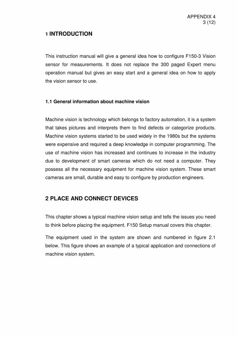
APPENDIX 4 4 (12)
Figure 2.1 Using the F150 to check for package defects.
Devices in the figure are numbered and the following will introduce and explain
the essential characteristics and special considerations for the placement of the
devices.
1. F150 Vision Mate Controller
The F150 Controller is the core of the system that handles the interpretation of
the picture provided by the camera and decides according to set rules if the part
is accepted or not. It incorporates the inputs and outputs to sensors and logic
controllers, so it should be located in a place that allows easy connection to this
equipment. F150 must be installed in a specific orientation and have a minimum
clearance of 50 mm above and below to improve heat dissipation. There should
be 200 mm space between the controller and power cables to avoid electrical
noise.
2. F150-S1A Camera
The camera is responsible for taking the pictures and sending them to the F150
Controller. Special consideration for the placement of the camera must be given
due to the importance of clear image and gaining the needed information from
the picture. Accidental knocks may change the orientation of the camera so
APPENDIX 4 5 (12)
rigid attaching is important. Camera case is connected to internal circuit 0V line
and should not be grounded to avoid noise interference.
3. Ikegami Video Monitor
The video monitor is to be placed in an accessible place to be able to monitor
the function of the camera and to adjust the settings of the controller. The
monitor is encased in a metal cover which is connected to the internal circuit 0V
line and it should not be grounded to avoid interference. Attaching should be
done avoiding metal screws/fasteners.
4. F150-KP Console
The console is used to configure the controller to function as needed. It should
be readily available for using and have a location where it can be put safely
when not in use.
5. S82K-03024 Power supply
Care must be taken in the placement of the power supply as hazardous
voltages are involved (230VAC). Ask your supervisor first, as you may not have
authorization to handle 230V equipment.
2.1 Before placing the equipment
When choosing the placement for the equipment, think at least the following
basic prerequisites:
• Can the equipment function as needed?
• Is there concern that accidental knocks may happen?
• Can other machinery disturb the equipment?
• Does the equipment obstruct access to other equipment?
• Can the equipment placement cause danger to people?
APPENDIX 4 6 (12)
These are just examples of possible questions. Mostly try to use your common
sense to assess practical locations.
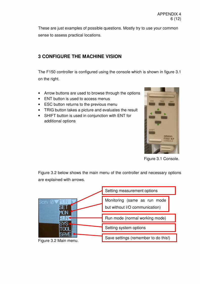
3 CONFIGURE THE MACHINE VISION
The F150 controller is configured using the console which is shown in figure 3.1
on the right.
• Arrow buttons are used to browse through the options • ENT button is used to access menus • ESC button returns to the previous menu • TRIG button takes a picture and evaluates the result • SHIFT button is used in conjunction with ENT for
additional options
Figure 3.1 Console.
Figure 3.2 below shows the main menu of the controller and necessary options
are explained with arrows.
Figure 3.2 Main menu.
Monitoring (same as run mode
but without I/O communication)
Setting measurement options
Save settings (remember to do this!)
Setting system options
Run mode (normal working mode)
APPENDIX 4 7 (12)
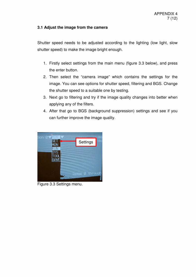
3.1 Adjust the image from the camera
Shutter speed needs to be adjusted according to the lighting (low light, slow
shutter speed) to make the image bright enough.
1. Firstly select settings from the main menu (figure 3.3 below), and press
the enter button.
2. Then select the “camera image” which contains the settings for the
image. You can see options for shutter speed, filtering and BGS. Change
the shutter speed to a suitable one by testing.
3. Next go to filtering and try if the image quality changes into better when
applying any of the filters.
4. After that go to BGS (background suppression) settings and see if you
can further improve the image quality.
Figure 3.3 Settings menu.
Settings
APPENDIX 4 8 (12)
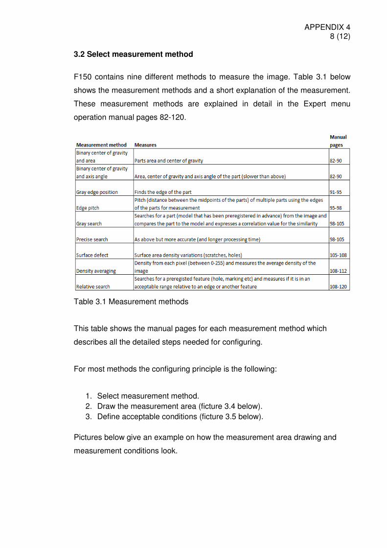
3.2 Select measurement method
F150 contains nine different methods to measure the image. Table 3.1 below
shows the measurement methods and a short explanation of the measurement.
These measurement methods are explained in detail in the Expert menu
operation manual pages 82-120.
Table 3.1 Measurement methods
This table shows the manual pages for each measurement method which
describes all the detailed steps needed for configuring.
For most methods the configuring principle is the following:
1. Select measurement method. 2. Draw the measurement area (ficture 3.4 below). 3. Define acceptable conditions (ficture 3.5 below).
Pictures below give an example on how the measurement area drawing and
measurement conditions look.
APPENDIX 4 9 (12)
Figure 3.4 Measurement area Figure 3.5 Measurement settings
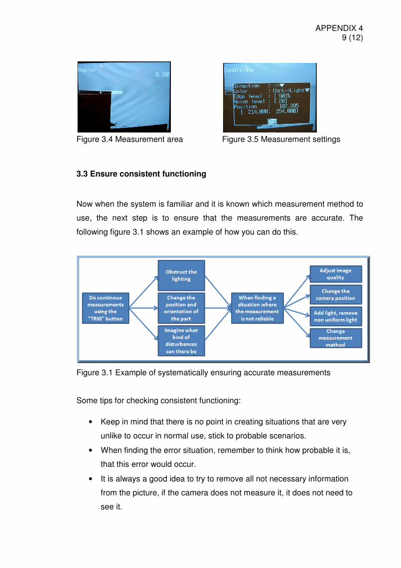
3.3 Ensure consistent functioning
Now when the system is familiar and it is known which measurement method to
use, the next step is to ensure that the measurements are accurate. The
following figure 3.1 shows an example of how you can do this.
Figure 3.1 Example of systematically ensuring accurate measurements
Some tips for checking consistent functioning:
• Keep in mind that there is no point in creating situations that are very
unlike to occur in normal use, stick to probable scenarios.
• When finding the error situation, remember to think how probable it is,
that this error would occur.
• It is always a good idea to try to remove all not necessary information
from the picture, if the camera does not measure it, it does not need to
see it.
APPENDIX 4 10 (12)
• If some measurement method seems to work unreliably with the
available equipment, think of another measurement method.
4 CONNECT TO OTHER DEVICES
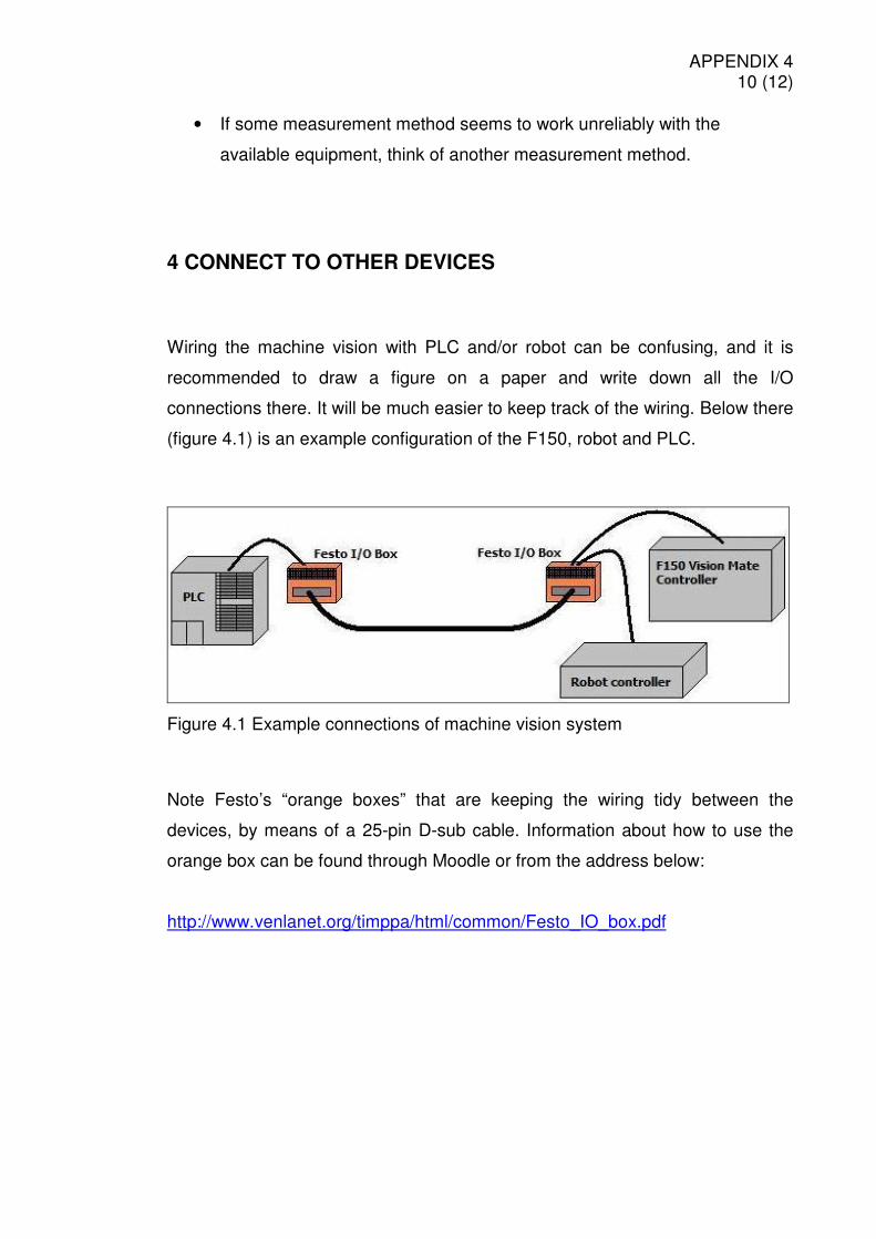
Wiring the machine vision with PLC and/or robot can be confusing, and it is
recommended to draw a figure on a paper and write down all the I/O
connections there. It will be much easier to keep track of the wiring. Below there
(figure 4.1) is an example configuration of the F150, robot and PLC.
Figure 4.1 Example connections of machine vision system
Note Festo’s “orange boxes” that are keeping the wiring tidy between the
devices, by means of a 25-pin D-sub cable. Information about how to use the
orange box can be found through Moodle or from the address below:
http://www.venlanet.org/timppa/html/common/Festo_IO_box.pdf
APPENDIX 4 11 (12)
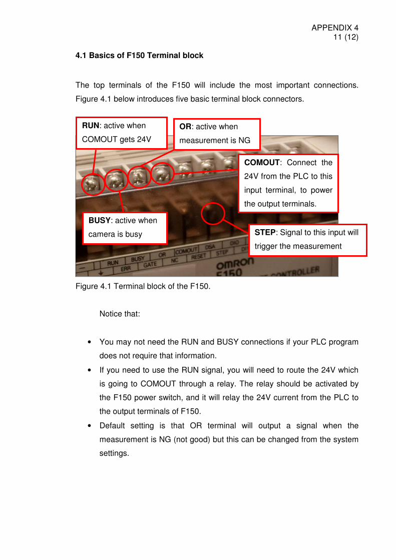
4.1 Basics of F150 Terminal block
The top terminals of the F150 will include the most important connections.
Figure 4.1 below introduces five basic terminal block connectors.
Figure 4.1 Terminal block of the F150.
Notice that:
• You may not need the RUN and BUSY connections if your PLC program
does not require that information.
• If you need to use the RUN signal, you will need to route the 24V which
is going to COMOUT through a relay. The relay should be activated by
the F150 power switch, and it will relay the 24V current from the PLC to
the output terminals of F150.
• Default setting is that OR terminal will output a signal when the
measurement is NG (not good) but this can be changed from the system
settings.
RUN: active when
COMOUT gets 24V
BUSY: active when
camera is busy
OR: active when
measurement is NG
COMOUT: Connect the
24V from the PLC to this
input terminal, to power
the output terminals.
STEP: Signal to this input will
trigger the measurement

APPENDIX 4 12 (12)
Detailed information about the terminal blocks and additional connectors can be
found from the Setup manual pages 29-34, and Expert menu operation manual
pages 183-195.
4.2 Machine vision configured
Now the system should be ready to be used with the PLC and/or robot.
Continue by creating the programs and enjoy the results of your work.