Embed Size (px)
Citation preview

Employee Turnover: Less is Not Necessarily More?*
Mark N. Harris#, Kam Ki Tang‡ and Yi-Ping Tseng†
# Department of Econometrics and Business Statistics, Monash University, Australia
† Melbourne Institute of Applied Economic and Social Research, University of Melbourne, Australia
‡ School of Economics, University of Queensland, Australia
September 2003
JEL Classification: J41, J63 Key words: Employee turnover, productivity, firm specific human capital, job matching, panel data, coordination.
* This paper is the result of work being undertaken as part of a collaborative research program entitled: “The
Performance of Australian Enterprises: Innovation, Productivity and Profitability”. The project is generously
supported by the Australian Research Council and the following collaborative partners: the Australian Tax
Office, the Commonwealth Office of Small Business, IBIS Business Information Pty Ltd, the Productivity
Commission, and the Victorian Department of State Development. The views expressed in this paper,
however, represent those of the authors and are not necessarily shared by the collaborative partners.
Corresponding author: Kam-Ki Tang. School of Economics, University of Queensland, QLD 4072, Australia.
Telephone: (617) 3365 9796; fax: (617) 3365 7299; email: [email protected]

1
Abstract
Theoretical studies have suggested firm specific human capital and job matching as the
major, but opposite, mechanisms through which employee turnover affects labour
productivity. This study finds that the former dominates when turnover is high, while the
latter dominates when turnover is low. The optimal turnover rate that maximises productivity
is about 0.22 per annum. Bringing the observed turnover rates in the sample to the optimal
level increases the average productivity by 1.1 per cent. The large gap between the observed
and the optimal rate could be explained by the lack of decision coordination between agents
in labour markets.
1 Introduction
It is widely acknowledged in the business community that human resources are an invaluable
firm asset (see, for example, Business Asia, 1999; Business Times, 2000). Therefore, it is
logical to assume that the flow of this valuable asset − employee turnover − will play a
crucial role in firm performance. Indeed, firms (and employees) are burdened with turnover
problems in both good and adverse economic climates. During economic upturns, employee
churning represents one of the greatest difficulties in business management. For instance,
during the “new economy” boom in the U.S., nearly a quarter of workers were reported to
have average tenure of less than a year (Economist 2000).1 On the other hand, during
economic downturns, trimming operating costs through job retrenchment in order to maintain
a firm’s share value is a typical phenomenon. Nevertheless, downsizing is not a painless
option for firms, as they are likely to suffer adverse consequences, such as low levels of
morality and loyalty amongst the remaining staff. Moreover, firms also bear the risk of not

2
being able to quickly re-establish the workforce should the economy rebound more swiftly
than anticipated.
As a consequence, employee turnover has been extensively researched across a number of
disciplines, including: psychology; sociology; management; and economics. Each discipline
has its own focus and, accordingly, employs different research methodologies. Psychologists
and sociologists, for example, are generally interested in the motivations behind quitting,
such as job satisfaction, organisational commitment and job involvement (Carsten and
Spector, 1987; Muchinsky and Tuttle, 1979). Empirical work in these fields typically
involves case studies using survey data of individual firms or organisations.
In the discipline of management study, high staff turnover has been of great and continuous
concern (as typified by Mok and Luk, 1995, and the symposium in Human Resource
Management Review, 9(4), 1999). Similar to the practice in psychology and sociology,
researchers heavily draw on event, or case, studies. While reducing employee turnover is a
managerial objective for some firms, the converse is true for others. For example, legal
restrictions and obligations in recruitment and dismissal could prohibit firms from
maintaining a flexible workforce size, a situation more common in unionised sectors
(Lucifora 1998). The industrial reforms and privatisation in many developed nations were
aimed, at least in part, at increasing the flexibility of labour markets.
In contrast, economists focus mainly on the implications of turnover on unemployment. A
strand of matching theories has been developed extensively to explain equilibrium
unemployment, wages and vacancies (Lucas and Prescott 1974; Lilien 1982). National
aggregate time series data are typically employed in this line of research. For recent surveys
1 High-tech industries as well as the low-tech ones, such as retailing, food services and call centres, experienced
the problem.

3
on matching theories and their applications see Petrongolo and Pissarides (2001) and the
symposium in Review of Economic Studies, 61(3) 1994.
Despite turnover being considered crucial to human resource management and production,
there is little quantitative research on the effect of turnover on labour productivity (hereafter
“productivity” unless specified otherwise).2 This omission is possibly due to the lack of firm
level data on both production and turnover. Moreover, firm level data are typically restricted
to individual organisations, prohibiting researchers from drawing general conclusions.3
Utilizing a recently released firm-level panel data set, based on the Australian Business
Longitudinal Survey (BLS), this paper is therefore able to provide a new dimension to the
literature. The BLS data provide an objective measure of value-added, which is comparable
across firms operating in a broad spectrum of industries. Conditional on firm level factor
inputs and other firm characteristics, the impacts of employee turnover on productivity are
investigated. The results suggest that employee turnover has a statistically significant and
quantitatively large, but more importantly, non-linear effect on productivity. From the results
it is possible to estimate the optimal turnover rate − the rate that maximises productivity,
keeping other factors constant − which was found to be around 0.22 per annum. As the
employee turnover rate is defined here as the average of total number of employees newly
recruited and departed within a period, relative to the average number of employees over the
2 McLaughlin (1990) examines the relationship between turnover type (quit or layoff) and economy-wide
general productivity growth, but not productivity of individual firms. Shepard et al. (1996) make use of
survey data to estimate the total factor productivity of the pharmaceutical industry; nevertheless, their study is
only concerned with the effect of flexible working hours and not turnover.
3 For instance, Borland (1997) studies the turnover of a medium-size city-based law firm, Iverson (1999)
examines voluntary turnover of an Australian public hospital, and Glenn, McGarrity and Weller (2001) focus
on major league baseball in the U.S. However, all three studies do not cover the production aspect of the
examined organisation.

4
period, the highest productivity is where about 22 per cent of total employees changed over
the one-year period. The estimated optimal rate is much higher than that typically observed in
the sample (the median turnover rate is about 14 per cent). Using a theoretical model, it is
shown that the lack of coordination between agents in labour markets can lead them choosing
a turnover rate far below the optimal level. The intuition is that the possibility for an
employer to find a more productive staff (or an employee for a more rewarding job) is related
to the rate of job-worker separations in other firms. Without sufficient information about the
intended decisions of others, agents will make changes at sub-optimal rates.
The empirical results also suggest that if firms bring their turnover rates to the optimal level,
average productivity will increase by just over 1 per cent. These results have clear policy
implications. For instance, if the observed turnover rate is substantially below the estimated
optimal rate and if institutional rigidity in the labour market is the main cause of that,
deregulation may be warranted.
The rest of the paper is structured as follows. Section 2 reviews two main contending theories
about the linkage between employee turnover and productivity, and formulates the concept of
the optimal turnover rate. In Section 3 the econometric model and the data are briefly
described. Section 4 presents the empirical results and Section 5 concludes. Appendix A
provides details of the data, including summary statistics. Appendix B presents a theoretical
model to account for the empirical findings.
2 Theories of Employee Turnover and Productivity
There are two main theories on how employee turnover can affect productivity. Firstly, there
is the firm specific human capital (FSHC) theory, pioneered by Becker (1975). This asserts
that if firms need to bear the cost of training, their incentives to provide staff training will be
lowered by high turnover rates. The incentive will be even weaker when firm specific and

5
general training are less separable, as employees have lower opportunity costs of quitting
(Lynch 1993). Consequently, productivity falls as turnover increases. Even if FSHC is bred
through learning-by-doing, its accumulation remains positively related to employees’ tenure.
As a result, a higher turnover rate will still lead to lower productivity.
In addition to the direct loss of human capital embodied in the leavers, there are other
negative impacts of turnover on productivity. Besides the output forgone during the vacant
and training period, the administrative resources used in separation, recruitment and training
could have been invested in other aspects of the production process.4 Moreover, high
employee turnover could adversely affect the morale of the organisation. Using a controlled
experiment, Sheehan (1993) records that the leavers alter the perceptions of the stayers about
the organisation and therefore negatively affect its productivity. As a consequence, warranted
(from an employer’s perspective) but involuntary job separation could trigger unwarranted
voluntary employee departure − a snowball effect.5
On the opposite side of the debate, is the job matching theory established by Burdett (1978)
and Jovanovic (1979a; 1979b). The key insight of this theory is that firms will search for
employees and job seekers will search for firms until there is a good match for both parties.
However, the conditions for an optimal matching may change over time, leading to
continuous reallocation of labour. For instance, a firm that has upgraded its production
technology will substitute skilled for unskilled labour (for a recent survey on this topic, see
4 It has been reported that the cost of losing an employee is between half to one and a half times the employee’s
annual salary (Economist 2000).
5 During the economic downturn in the U.S. in 2001, executives in Charles Schwab and Cisco were reportedly
cutting down their own salaries and setting up charitable funds for laid off staff in order to maintain the
morale of the remaining employees (Economist 2001). Both companies’ efforts were apparently well
received. Fortune (2002) ranked Cisco and Charles Schwab as the 15th and 46th best companies to work for in
2001, respectively, despite Cisco was reported laying off 5,500 staff while Charles Schwab 3,800 staff.

6
Ahn, 2001). Moreover, established firms also need ‘new blood’ to provide fresh stimulus to
the status quo. On the other hand, a worker who has acquired higher qualifications via
education, training, or learning-by-doing may seek a better career opportunity.
Regular employee turnover helps both employers and employees avoid being locked in sub-
optimal matches permanently. For instance, the estimated cost of a poor hiring decision is 30
per cent of the first year’s potential earning and even higher if the mistake is not corrected
within six months, according to a study by the U.S. Department of Labor (cited in Abbasi and
Hollman 2000).
Another factor that compounds the effect of turnover on productivity is knowledge spillover
between firms (Cooper 2001). Knowledge spillover is more significant if human capital is
portable across firms or even industries. Megna and Klock (1993) find that increasing
research input by one semi-conductor firm will increase the productivity of rival firms due to
labour migration. Finally, Borland (1997) suggests that involuntary turnover can be used as a
mechanism to maintain employees’ incentives. In short, matching theory suggests that higher
turnover aids productivity.
Although FSHC theory and job matching theory suggest opposite effects of turnover on
productivity, one does not necessarily invalidate the other. In fact, there is empirical evidence
supporting the coexistence of both effects, albeit the effect of FSHC appears to dominate
(Glenn et al. 2001). The two theories essentially answer the question of how to balance the
stability and flexibility of the labour force. It is the contention here, that given that FSHC and
job matching have opposite effects on productivity, there is a distinct possibility that a certain
turnover rate will maximise productivity. A scenario, in which such an optimal turnover rate
exists, is where productivity is a non-linear – specifically quadratic concave function, of
turnover.

7
3 Data, Empirical Model and Estimation Method
3.1 Business Longitudinal Survey
The BLS is a random sample of business units selected from the Australian Bureau of
Statistics business register for inclusion in the first year of the survey. The sample was
stratified by industry and firm size. The sample was selected with the aim of being
representative of all businesses (excluding government agents, public utilities and public
services). The focus is on a balanced panel of small and medium sized businesses. After
excluding businesses with deficient data records, 2,435 businesses are left in our sample.
Summary statistics and variable definitions are presented in Appendix A.
This data source is unique in that it provides firm-level data, including an objective measure
of value-added, and structural firm characteristics. Moreover, individual firms are tracked
over a four-year period from 1994/5 to 1997/8. The panel nature of the data allows us to
investigate the correlation between firm characteristics and productivity, whilst
simultaneously taking into account unobserved firm heterogeneity.
Due to data inconsistencies however, focus is on a sub-two-year panel. Also, some firms
reported employee turnover rates well in excess of 1 (the maximum value of turnover rate in
the data set is 41!). Since the figure is supposed to measure the turnover of non-causal
workers only, the accuracy of these high value responses is questionable. It is suspected that
most of those firms that reported a high turnover rate might have mistakenly included the
number of newly hired and ceased “casual” employees in their counting. In that case,
considerable measurement errors would be introduced. There is no clear pattern on the
characteristics of firms with very high reported turnover rates. Thus, observations whose
employee turnover rates are greater than 0.8 (equivalent to 5% of total sample) are excluded

8
from the estimations. As the cut-off point of 0.8 is relatively arbitrary, different cut-off points
are experimented with as robustness checks.
3.2 The Empirical Model
The empirical model is a productivity function derived from a Cobb-Douglas production
function. Using capital-labour ratio, employee turnover and other firm characteristics to
explain productivity, the regression model has the following form:6
20 1 2 1 2( / ) ln( / ) lnit it it it it it it i it i itln V L K L L T T u eβ β β δ δ= + + + + + + + +φW θZ (1)
where itV is value-added of firm i in year t, and itK , itL and itT denote capital, labour
(effective full time employees) and employee turnover rate, respectively. Employee turnover
rate is measured by the average of new employees and ceased non-casual employees divided
by average non-casual employees at the end of year t and t-1. Unobserved firm heterogeneity
and idiosyncratic disturbances, are respectively denoted iu and ite . Wi is a vector of time
invariant firm characteristics, including dummies for family business, incorporation, industry,
and firm age and firm size at the first observation year. Zit denotes a vector of time variant
covariates including employment arrangements (ratios of employment on individual contract,
unregistered and registered enterprise agreements), other employee related variables
(managers to total employees ratio, part-time to total employees ratio, union dummies) and
6 It has been verified that terms with orders higher than two are insignificant. Furthermore, if there are feedback
effects of productivity on the turnover rate, one should include lagged terms of T in the equation and/or set up
a system of equations. For instance, using U.S. data, Azfar and Danninger (2001) find that employees
participating in profit-sharing schemes are less likely to separate from their jobs, facilitating the accumulation
of FSHC. However, the short time span of our panel data prohibits us from taking this into account in the
empirical analysis.

9
other firm characteristics (innovation status in the previous year, borrowing rate at the end of
previous financial year, and export status).
Equation (1) can be viewed as a (conditional) productivity-turnover curve (PT).7 The five
scenarios regarding the signs of δ1 and δ2 and, thus, the shape of the PT curve and the optimal
turnover rate are summarised in Table 1.
Table 1. Various Scenarios of the Productivity-Turnover Curve
Scenario Shape of PT curve
( 0T ≥ )
Interpretation Optimal
turnover rate
1 2 0δ δ= = Horizontal FSHC and job matching effects
cancel each other
Undefined
1 20, 0δ δ> < n-shaped Job matching effects dominate
when T is small, while FSHC
effects dominate when T is large
1
22δδ
−
1 20, 0δ δ< > U-shaped FSHC effects dominate when T is
small, while job matching effects
dominate when T is large
Undefined
1 2
1 2
0, 0,0
δ δδ δ≥ ≥+ ≠
Upward sloping Job matching effects dominate Undefined
1 2
1 2
0, 0,0
δ δδ δ≤ ≤+ ≠
Downward sloping FSHC effects dominate 0

10
A priori, one would expect δ1 > 0 and δ2 < 0, giving rise to an n-shaped PT curve. This is
because, when turnover is very low, job-worker match is unlikely to be optimal as technology
and worker characteristics change continuously. Hence, the marginal benefit of increasing the
labour market flexibility overwhelms the marginal cost of forgoing some FSHC. As a result,
productivity rises with the turnover rate. Due to the law of diminishing marginal returns, the
gain in productivity lessens as turnover increases. Eventually the two effects will net out;
further increases in turnover will then lead to a fall in productivity.
In the case of an n-shaped PT curve, the optimal turnover rate is equal to 0.5δ1/δ2. The rate is
not necessarily optimal from the perspective of firms, as competent employees may leave for
a better job opportunity. Neither is it necessarily optimal from the perspective of employees,
as there may be involuntary departure. In essence, turnover represents the fact that firms are
sorting workers and, reciprocally, workers are sorting firms. As a result, the estimated
optimal rate should be interpreted from the production perspective of the economy as a
whole. Moreover, the measurement does not take into account the hidden social costs of
turnover, such as public expenses on re-training and unemployment benefits, and the
searching costs borne by job seekers, and for that matter, hidden social benefits such as
higher social mobility.
3.3 Estimation Methods
Following Wooldridge (2002, p.252) the unobserved effects of equation (2) are treated as
random, since the cross-sectional component of the data is a random drawing from the full
population. Moreover, a fixed-effects approach precludes the identification of the effects of
7 The effects of turnover on productivity are essentially the same as those on value-added as factor inputs have
been controlled for.

11
any time-invariant variables in the model. Consistency of this approach relies on the
assumption that, conditional on all of the explanatory variables in the model, the expected
value of the unobserved effect is zero. Hausman tests suggested that there was some evidence
that this assumption might not be valid. If this is the case, it is possible to gain consistent
parameter estimates within a random effects framework following the Generalised Method of
Moments estimators suggested by Hausman and Taylor (1981), Amemiya and MaCurdy
(1986) and Breusch, Mizon and Schmidt (1989). However, possibly due to a lack of across-
time variation in most of the explanatory variables, none of these methods yielded
appropriate parameter estimates according to the Sargan criteria of appropriate moment
conditions.
4 Empirical Results
4.1 Results of Production Function Estimation
Table 2 reports the estimation results for the base case – the sample with cut-off point of 0.8
– and also results for the full sample. For the base case, two models are estimated; with and
without the restriction of constant returns to scale (CRS). The results indicate that the CRS
restriction cannot be rejected, as the coefficient of log labour in the unrestricted model is not
significantly different from zero. Accordingly, focus is on the CRS results for the base case in
the following discussion (the middle two columns).
The coefficient of log capital is very small. This is not surprising due to the use of non-
current assets as a proxy of capital (see Appendix A for details). This argument gains support
from the negative coefficients of firm age dummies in that the under-estimation of capital is

12
larger for older firms.8 Since both capital and firm age variables are included as control
variables, the mismeasurement of capital should not unduly bias the coefficient of employee
turnover.
The coefficient of the ratio of employees on individual contract is significantly positive. This
is expected as individual contracts and agreements tend to be more commonly used with
more skilled employees, and also because such agreements tend to be used in tandem with
performance-based pay incentives. Although it is widely believed that registered enterprise
agreements are positively correlated with productivity (Tseng and Wooden 2001), the results
here exhibit the expected sign but the effect is not precisely estimated. Interestingly,
productivity is higher for unionised firms and it is particularly significant for those with more
than 50 per cent of employees being union members.
The coefficient of the lagged borrowing rate is, as expected, positive, and significant. It is
consistent with the theory that the pressure of paying back debts motivates greater efforts in
production (Nickell, Wadhwani and Wall 1992). Manager to total employee ratio appears to
have no effect on productivity, while the negative effects of part-time to full-time employee
ratio is marginally significant. The latter result is probably due to the fact that part-time
workers accumulate less human capital than their full-time counterparts.
The coefficient of innovation in the previous year is insignificant, possibly due to the
potentially longer lags involved. Export firms have higher productivity; highly productive
businesses are more likely to survive in highly competitive international markets and trade
may prompt faster absorption of new foreign technologies. Non-family businesses, on
average, exhibit 16 per cent higher (labour) productivity than family businesses, whereas
8 If there is no underestimation of capital stock, other things equal, older firms are likely to have higher
productivity due to accumulation of experience.

13
incorporated firms are 13 per cent higher than non-incorporated ones. The result signifies the
importance of corporate governance, as non-family businesses and incorporated firms are
typically subject to tighter scrutiny than their counterparts. Medium and medium large firms
have 15 and 20 per cent higher productivity, respectively, than small firms.

14
Table 2 Estimation Results from Random Effect Models
Restrict CRS Restrict CRS Not restrict CRS Full sample Turnover<0.8 Turnover<0.8 Coef. Std. err. Coef. Std. err. Coef. Std. err. Log Capital-labour ratio 0.189* 0.009 0.188* 0.009 0.184* 0.009 Log Labour 0.031 0.023 Turnover Rate -0.016 0.027 0.182 0.113 0.169 0.112 Turnover Rate squared -0.001 0.004 -0.418* 0.182 -0.399* 0.181 Ratio of employment on 0.131* 0.025 0.133* 0.026 0.128* 0.026
Ratio of employment on -0.006 0.031 0.004 0.032 0.001 0.032
Ratio of Employment on 0.057 0.045 0.062 0.047 0.056 0.047
Ratio of manager to total 0.095 0.076 0.098 0.078 0.144# 0.084 Ratio of part-time to total -0.044 0.040 -0.075# 0.041 -0.055 0.043 Union Dummy (1-49%) 0.031 0.025 0.026 0.025 0.022 0.026 Union Dummy (50%+) 0.086* 0.038 0.082* 0.038 0.077* 0.039 Family business -0.163* 0.024 -0.164* 0.024 -0.166* 0.025 Incorporated 0.135* 0.026 0.132* 0.027 0.130* 0.027 Export 0.106* 0.023 0.103* 0.024 0.097* 0.024 Innovation (t-1) 0.005 0.015 0.000 0.016 0.000 0.016 Borrowing rate (t-1) 0.011* 0.005 0.011* 0.005 0.011 0.005 Size: medium 0.154* 0.028 0.153* 0.029 0.116* 0.041 Size: medium-Large 0.199* 0.052 0.191* 0.053 0.125# 0.075 Age (less than 2 years) -0.171* 0.050 -0.171* 0.051 -0.170* 0.052 Age (2 to less than 5 years) -0.060 0.038 -0.061 0.040 -0.057 0.040 Age (5 to less than 10 years) -0.017 0.032 -0.014 0.033 -0.013 0.033 Age (10 to less than 20 years) -0.018 0.030 -0.022 0.031 -0.020 0.032 Constant 3.282* 0.056 3.289* 0.058 3.229* 0.080 Industry dummies Yes Yes Yes
uσ 0.472 0.481 0.482
eσ 0.301 0.297 0.287
ρ σ σ σ= +u u e2 2 2c h 0.711 0.725 0.739
Number of observations 4472 4249 4249 Number of firms 2357 2311 2311
231χ test for overall significance 1295.21 1235 1194.84
Note: * and # indicate significance at 5% and 10% level, respectively.

15
4.2 Employee Turnover and Productivity
Focus now turns to the impact of turnover on productivity. The coefficients of employee
turnover rate and its square are jointly significant at 5 per cent significance level, although
individually the coefficient of the turnover rate has not been precisely estimated. The two
coefficients are positively and negatively signed, respectively, implying an n-shaped PT
profile. It indicates that, job matching effects dominate when turnover is low, whereas FSHC
effects dominate as turnover increases. For the base case, the imputed optimal turnover rate is
equal to 0.22.9 This figure changes very little even if the restriction of constant returns to
scale is imposed in estimations.
Although the coefficients of other explanatory variables for the full and trimmed samples are
not markedly different, the same is not true of those of turnover rate and turnover rate
squared. This indicates that the extremely large turnover rates are likely to be genuine
outliers, justifying their exclusion. However, notwithstanding this result, the estimated
optimal turnover rates are remarkably stable across samples with different cut-off points
(Table 3), lying between 0.214 and 0.231, even though the coefficient are sensitive to the
choice of estimation sample. Firms with a turnover rate higher than 0.5 are likely to be
“outliers” as our definition of turnover excluded casual workers.10 Since the measurement
errors are likely to be larger at the top end of the distribution, the effect of employee turnover
rate weakens as the cut-off point increases. To balance between minimizing the measurement
9 Using 1,000 Bootstrap replications, 93.1 per cent of the replications yielded n-shaped PT curves. The 95 per
cent confidence interval for the base case optimal turnover rate is (0.052, 0.334).
10 As a casual benchmark, policy advisers working for the Australian Government are reported to have very high
turnover rates, mainly due to long hours, high stress and lack of a clear career path (Patrick 2002). Their
turnover rate was found to range from 29 per cent to 47 per cent under the Keating government (1991−1996).
16
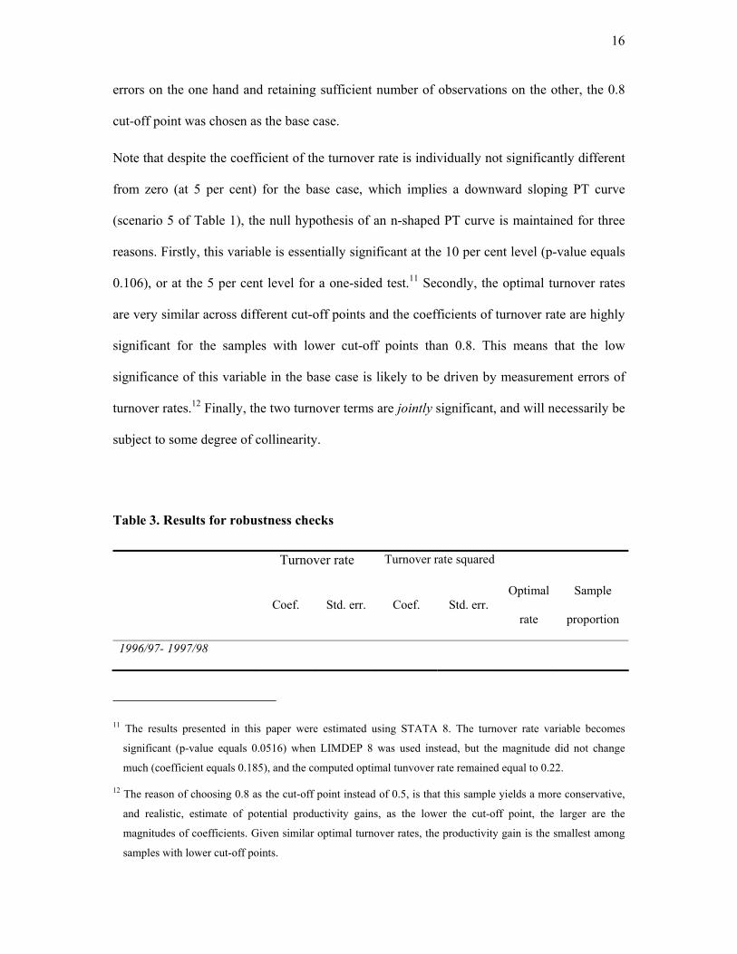
errors on the one hand and retaining sufficient number of observations on the other, the 0.8
cut-off point was chosen as the base case.
Note that despite the coefficient of the turnover rate is individually not significantly different
from zero (at 5 per cent) for the base case, which implies a downward sloping PT curve
(scenario 5 of Table 1), the null hypothesis of an n-shaped PT curve is maintained for three
reasons. Firstly, this variable is essentially significant at the 10 per cent level (p-value equals
0.106), or at the 5 per cent level for a one-sided test.11 Secondly, the optimal turnover rates
are very similar across different cut-off points and the coefficients of turnover rate are highly
significant for the samples with lower cut-off points than 0.8. This means that the low
significance of this variable in the base case is likely to be driven by measurement errors of
turnover rates.12 Finally, the two turnover terms are jointly significant, and will necessarily be
subject to some degree of collinearity.
Table 3. Results for robustness checks
Turnover rate Turnover rate squared
Coef. Std. err. Coef. Std. err. Optimal
rate
Sample
proportion
1996/97- 1997/98
11 The results presented in this paper were estimated using STATA 8. The turnover rate variable becomes
significant (p-value equals 0.0516) when LIMDEP 8 was used instead, but the magnitude did not change
much (coefficient equals 0.185), and the computed optimal tunvover rate remained equal to 0.22.
12 The reason of choosing 0.8 as the cut-off point instead of 0.5, is that this sample yields a more conservative,
and realistic, estimate of potential productivity gains, as the lower the cut-off point, the larger are the
magnitudes of coefficients. Given similar optimal turnover rates, the productivity gain is the smallest among
samples with lower cut-off points.

17
Turnover<0.5 0.435 0.175 -1.001 0.422 0.217 0.872
Turnover<0.6 0.411 0.146 -0.962 0.298 0.214 0.914
Turnover<0.7 0.178 0.124 -0.385 0.219 0.231 0.938
Turnover<0.8 (base case) 0.182 0.113 -0.418 0.182 0.218 0.950
Full sample -0.016 0.027 -0.001 0.004 0 1.0
1995/6 - 1997/98
Turnover<0.8 0.153 0.084 -0.244 0.136 0.313 0.951
Table 4. Estimation results by industry and firm size
Turnover rate Turnover rate squared
Coef. Std. err. Coef. Std. err.Optimal
rate
Number of
observations
Manufacturing 0.393 0.140 -0.821 0.226 0.239 1825
Wholesale trade 0.317 0.326 -0.711 0.550 0.223 792
Retail trade 0.834 0.301 -1.251 0.473 0.333 440
Small firms 0.398 0.144 -0.925 0.240 0.215 2082
Medium and medium-large
firms -0.170 0.176 0.254 0.273 − 2167
The model is also estimated by industry and firm size (with the choices of such being driven
by effective sample sizes) and the results are presented in Table 4. The retail trade industry
has the highest optimal turnover rate of 0.33, compared to 0.24 and 0.22 of the manufacturing
and wholesale trade industries, respectively. The retail trade industry also faces the greatest
productivity loss from deviating from the optimal rate as it has the steepest PT curve. Figure
1 illustrates the PT curve for three different samples (all, manufacturing and small firms). The

18
diagram is a plot of log productivity against turnover rate. The PT curve can be read as that,
in the base case, increasing employee turnover rate from 0 to the optimal point (0.22), on
average, raises productivity by 1.95 per cent.
Figure 1. Productivity-Turnover Curve
-0.02
0
0.02
0.04
0.06
0 0.05 0.1 0.15 0.2 0.25 0.3 0.35 0.4 0.45 0.5
turnover rate
log
labo
ur p
rodu
ctiv
ity
all firms (base case)
manufacturing
small firms
The median turnover rate for the base case sample is 0.136, which is well below the optimal
rate.13 A possible explanation for the large gap between the estimated optimal rate and the
sample median is the lack of coordination between agents (employers and employees) in the
labour market. For instance, when an employer is pondering whether to layoff an
unproductive employee, he/she needs to consider the chance of finding a better replacement
within a certain period of time. The chance depends on, amongst other factors, the turnover
13 The average turnover rate of the base case sample is 0.183. However, median is a more useful concept here
because the average figure is dominated by the high turnover rates of a handful of firms.
19
rates in other firms. Without sufficient information about the employment plan of each other,
agents will make changes at a rate lower than what would have been if information were fully
revealed. In Appendix B, a formal model is presented to elaborate this explanation. Another
plausible explanation is that there is an enormous amount of friction in the dismissal and
hiring process, such as legal restrictions. Yet another possible explanation is that employers
may be concerned about non-pecuniary compensation, such as a harmonious working
environment, which may or may not sufficiently compensate for inferior job matching. This
scenario is likely to be important for small and medium sized firms, which characterise the
BLS data.
While the finding cannot pin down exactly what factors attribute to the gap, it indicates how
much can be gained by bringing the turnover rate towards the optimal level. The average
productivity gain from closing the gap is equal to 1.1 per cent, which is the average increment
of productivity for the firms in the base sample if their turnover rates shift from observed to
the optimal values, weighted by the firms’ value added.14 Given that the steepest of the PT
curve increases with lower cut-off point, 1.1 per cent should be viewed as a lower bound
value.
Note that as the analysis in this paper is based on small and medium firms, it is not possible
to draw inferences to the population of all firms. Very large firms typically consist of many
sub-units, which could all be considered smaller “firms”. Therefore, within-firm mobility
14 Note that there is the possibility that lower productivity might lead to payroll retrenchment. However, if so,
this is likely to have an impact on staffing decisions with lags (for example, due to uncertainty in
distinguishing cyclical effects from long run declines in productivity, and measurement error in identifying
individual worker’s productivity in team production). Since the estimations use contemporaneous turnover
and productivity figures, any potential endogeneity will be alleviated.

20
may substitute between-firm mobility.15 Also, it is not possible to test the potential long-term
effects of turnover on productivity here due to data restrictions. For instance, unfavourable
comments on a firm spread by its involuntarily separated employees may damage its
corporate image and, thus, weaken its attraction to quality potential employees. Therefore,
employee turnover may have slightly stronger negative effect in the long run. However, this
reputation effect should not be significant for small and medium firms because of their
relative size in the labour market. To examine this long run effect (as well as any potential
reverse causation effect discussed in footnoted 11) requires the use of a longer panel.
5 Conclusions
This paper sets out to quantify the impact of employee turnover on productivity. Of the two
major theoretical arguments, FSHC theory asserts that high turnover lowers firms’ incentives
to provide staff training programs and consequently, reduces productivity. On the other hand,
job matching theory postulates that turnover can help employers and employees avoid being
locked in sub-optimal matches permanently, and therefore increases productivity. The
conflict between retaining workforce stability on the one hand, and flexibility on the other,
gives rise to the potential existence of an “optimal” turnover rate.
Using an Australian longitudinal data set, productivity was found to be a quadratic function
of turnover. The n-shaped PT curve is consistent with the intuition that job matching effects
dominate while turnover is low, whereas FSHC effects dominate while turnover is high. The
optimal turnover rate is estimated to be about 0.22. This result was robust to both estimation
method and sample (with the possible exception of the retail trade sector).
15 In a case study, Lazear (1992) finds that the pattern of within-firm turnover from job to job resembles that of
between-firm turnover.

21
The fact that the estimated optimal rate is much higher than the sample median of 0.14 raises
questions about whether there are institutional rigidities hindering resource allocation in the
labour market. Using a theoretical model, it is shown that the large turnover gap can be
explained by the lack of decision coordination between agents in the market. The empirical
results also indicate that higher productivity can be gained from narrowing this gap - average
productivity increase was estimated to be at least 1.1 per cent if the turnover rates across the
sampled firms are brought to the optimal level.

22
Appendix A: The Working Sample and Variable Definitions
The first wave of BLS was conducted in 1994/5, with a total effective sample size of 8,745
cases. The selection into the 1995/6 sample was not fully random. Businesses that had been
innovative in 1994/95, had exported goods or services in 1994/95, or had increased
employment by at least 10 per cent or sales by 25 per cent between 1993/94 and 1994/95,
were included in the sample. A random selection was then made on all remaining businesses.
These businesses were traced in the surveys of the subsequent two years. In order to maintain
the cross-sectional representativeness of each wave, a sample of about 800 businesses were
drawn from new businesses each year. The sample size in the second, third and fourth waves
are around 5,600. For detailed description of the BLS data set, see Tseng and Wooden
(2001). Due to confidentiality considerations, the complete BLS is not released to the public,
only the Confidentialised Unit Record File (CURF) is available. In the CURF, businesses
exceed 200 employees and another 30 businesses that are regarded as large enterprises using
criteria other than employment are excluded. This leaves around 4,200 businesses in the
balanced panel.
Deleting observations that had been heavily affected by imputation, as their inclusion would
impose artificial stability, further reduced the number of cases available for analysis.
Moreover, businesses in the finance and insurance industries were excluded because of
substantial differences in the measures of value-added and capital for these firms (and
effective sample sizes too small to undertake separate analyses on these groups). In addition,
observations with negative sales and negative liabilities were dropped, as were a small
number of cases where it was reported that there were no employees. In total, this left just
2,435 businesses in our sample. Summary statistics are presented in Table A.
The dependent and explanatory variables are briefly described as follows:

23
• ln itV (log value-added): Value-added is defined as sales − purchase + closing stock −
opening stock, in financial year t.
• ln itK (log capital): Capital is measured as the total book value of non-current assets plus
imputed leasing capital. As reported in Rogers (1999), the importance of leasing capital
relative to owned capital varies significantly with firm size and industry, suggesting that
leasing capital should be included if we are to accurately approximate the total value of
capital employed in the production process. Leasing capital is imputed from data on the
estimated value of rent, leasing and hiring expenses.16
• ln itL (log labour): Labour input is measured as the number of full-time equivalent
employees.17 Since employment is a point in time measure, measured at the end of the
survey period (the last pay period in June of each year), we use the average numbers of
full-time equivalent employees in year t and year t-1 for each business as their labour
input in year t.18
• itT (employee turnover rate): Employee turnover rate is measured by the average of new
employees and ceased non-casual employees divided by average non-casual employees at
the end of year t and t-1. The variables are only available from 1995/6 onwards.
16 Leasing capital is imputed using the following formula: leasing capital = leasing expenses/(0.05+r). The
depreciation rate of leasing capital is assumed to be 0.05. Ten-year Treasury bond rate is used as the discount
rate (r). See Rogers (1999) for more detailed discussion.
17 The BLS only provides data on the number of full-time and part-time employees while the number of work
hours is not available. The full-time equivalent calculation is thus based on estimated average work hours of
part-time and full-time employees for the workforce as a whole, as published by the ABS in its monthly
Labour Force publication (cat. no. 6203.0).
18 Capital is also a point in time measure. However, capital is far less variable than labour (especially when
measured in terms of its book value), and hence the coefficient of capital is not sensitive to switching between
flow and point-in-time measures.

24
Moreover, the questions for the calculation of labour turnover rate are slightly different in
1995/6 questionnaires.
• iW (time invariant control variables):
- Firm age dummies: this variable is to control for any bias associated with the
mismeasurement of capital, as well as to control for industry specific knowledge.19
- Industry dummies: industry dummies are included to control for industry specific
factors that may not be captured by the above variables.
• itZ (time variant control variables):
- Employment arrangement: there are three variables included in the regression
proportion of employees covered by individual contracts, by registered enterprise
agreements, and by unregistered enterprise agreements. The proportion of employees
covered by award only is omitted due to perfect multi-collinearity.
- Union dummies: these dummies indicate whether a majority or a minority of
employees are union members, respectively. A majority is defined as more than 50
per cent and a minority being more than zero but less than 50 per cent. The reference
category is businesses without any union members at all.
- Part-time employee to total employee ratio and manager to total employee ratio: the
effect of manager to total employee ratio is ambiguous because a higher ratio implies
employees being better monitored on the one hand, while facing more red tape on the
19 A source of measurement bias is the use of the book value of non-current assets. Using the book value will, in
general, lead to the underestimation of the true value of capital due to the treatment of depreciation. As firms get
older, the book value of capital is generally depreciated at a rate greater than the diminution in the true value of
the services provided by the capital stock.

25
other. The effect of part-time to total employee ratio is also ambiguous because part-
timers may be more efficient due to shorter work hours, but they may be less
productive due to less accumulation of human capital.
- A dummy variable that indicates whether a business was “innovative” in the previous
year: Innovation potentially has a long lag effect on productivity. Since the panel is
relatively short, in order to avoid losing observations, we include only a one-year lag.
Moreover, the definition of innovation is very board in the BLS. The coefficient of
innovation dummy is expected to be less significant than it should be.
- Dummy variables that indicate whether a business is a family business, or an
incorporated enterprise. The questions are asked at the first wave of the survey, so
both variables are time invariant.
- Borrowing rate: It is measured at the end of the previous financial year. This variable
is used to measure how highly geared a firm is.

26
Table A: Summary statistics
Full sample Trimmed sample
Variable Mean Std. Dev. Mean Std. Dev.
Log labour productivity 4.281 0.695 4.289 0.694
Log Capital-labour ratio 3.968 1.091 3.972 1.086
Log Labour 2.823 1.119 2.845 1.114
Turnover Rate 0.252 0.470 0.183 0.181
Ratio of Employment on individual
contract
0.251 0.365 0.254 0.367
Ratio of Employment on Unregistered
agreement
0.085 0.249 0.084 0.248
Ratio of Employment on Registered
agreement
0.068 0.218 0.069 0.218
Manager to total employee ratio 0.255 0.169 0.252 0.168
Ratio of part-time to total employee 0.202 0.282 0.195 0.276
Union Dummy (1-49%) 0.206 0.405 0.209 0.407
Union Dummy (50%+) 0.079 0.270 0.082 0.274
Family business 0.514 0.500 0.512 0.500
Incorporated 0.715 0.451 0.717 0.450
Export 0.271 0.444 0.272 0.445
Innovation (t-1) 0.292 0.455 0.293 0.455
Borrowing rate (t-1) 0.746 1.395 0.746 1.397
Medium 0.443 0.497 0.445 0.497
Medium-Large 0.066 0.248 0.065 0.247
Age (less than 2) 0.062 0.241 0.062 0.241
Age (2 to less than 5 years) 0.129 0.335 0.129 0.335
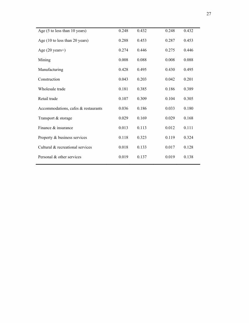
27
Age (5 to less than 10 years) 0.248 0.432 0.248 0.432
Age (10 to less than 20 years) 0.288 0.453 0.287 0.453
Age (20 years+) 0.274 0.446 0.275 0.446
Mining 0.008 0.088 0.008 0.088
Manufacturing 0.428 0.495 0.430 0.495
Construction 0.043 0.203 0.042 0.201
Wholesale trade 0.181 0.385 0.186 0.389
Retail trade 0.107 0.309 0.104 0.305
Accommodations, cafes & restaurants 0.036 0.186 0.033 0.180
Transport & storage 0.029 0.169 0.029 0.168
Finance & insurance 0.013 0.113 0.012 0.111
Property & business services 0.118 0.323 0.119 0.324
Cultural & recreational services 0.018 0.133 0.017 0.128
Personal & other services 0.019 0.137 0.019 0.138

28
Appendix B: A Simple Model of Optimal Turnover Rate and Coordination
The objective of developing this model is to provide a theoretical explanation for the
empirical finding in the main text. The model is not supposed to exhaust all possible
explanations. It focuses on only one element, namely the coordination problem between
firms.20 This element alone, as shown below, is sufficient to account for the apparently large
gap between the estimated optimal turnover rate and the sample median rate.
The model focuses on the steady state optimal employee turnover rate for a representative
firm. Therefore, it abstracts from adjustment issues. To simplify the analysis, we make a
number of assumptions:
(a) All separations are initiated and controlled by the firm. So there is no employee
churning. As explained later, churning can be modelled separately using a similar
framework.
(b) Production uses a Cobb-Douglas technology with a fixed capital to labour ratio for
both incumbents and newcomers. All workers use the same type of capital.
(c) The real wages received by both types of worker are fixed.
(d) The degree of job matching is random so that a worker who matches a vacancy in one
firm does not necessarily match the vacancies in other firms equally well. As a result,
firms are not competing with each other, and all firms benefit from having a larger
pool of job seekers.
(e) In every period the firm lays off a certain proportion of incumbents, in the hope of
replacing them with better-matched workers.
20 One can formulate similar arguments using the notion of imperfect information in the labour market and risk
adverseness of agents.

29
(f) All incumbents are identical and have the equal chance of being laid off. Therefore, in
terms of FSHC, there is a difference between incumbents and newcomers but not
amongst incumbents themselves. As a consequence, the output of incumbents depends
only on their average tenure but not on the distribution of tenures.21
The total number of staff for a representative firm, N, is normalized to one:
1 I H LN N N N= = + − (2)
where IN is the number of incumbents; HN the number of newly hired staff; LN the number
of incumbents being laid off in each period. In steady state, the total number of staff remains
constant, implying that H LN N= .
The turnover rate is
2
H LH
N N NN
θ += = . (3)
Given that the total number of staff is normalized to one and the capital to labour ratio is
constant, it implies that the capital stock is fixed. Therefore, the profit of the firm can be
written as a function of labour input:
( ) ( ) ( ) ( )2I L H I I L H H H LcA N N B N w N N w N N Nλ λπ = − + − − − − + (4)
where A is the productivity factor of incumbents; B the productivity factor of newcomers; Iw
and Hw are the real wage rates for incumbents and newcomers, respectively; c/2 the real cost
of hiring and laying off staff. Output price is normalized to one.
21 A possible justification for this assumption is that FSHC reaches its satiation level within a short tenure, so
that all incumbents are very similar.

30
The amount of FSHC an average incumbent can accumulate is negatively related to the
chance that she will be laid off in any given period and, thus, to the turnover rate. Here we
specify the productivity factor of incumbents as
(1 )A ασ θ= − (5)
where σ is a positive coefficient, and its value is positively related to the stock of capital. A
larger value of α represents a greater FSHC effect.
The productivity factor of newcomers is not a constant. The firm will try to select candidates
with a better job-match than an average incumbent. Otherwise, there would be no gain to lay
off experienced staff and find an inexperienced replacement. The average productivity of a
newcomer depends on the size of the pool of talent from which firms can pick their
candidates.22 If all firms are identical, then the size of the pool will be positively related to the
turnover rate in a representative firm. We specify an ad hoc relationship between them as
B βσθ= . (6)
The specifications of A and B have the same coefficient σ, because if there are not FSHC and
job matching effects, incumbents and freshmen are identical. A larger value of β represents a
greater job-matching effect. It is assumed that 1λ α+ < and 1λ β+ < .23
If there is no coordination between firms, each firm will treat B as a constant rather than a
function of θ. In the followings, we consider the two cases that firms do not coordinate and
coordinate, respectively.
Without coordination, the problem faced by the firm can be formulated as:
22 Here we implicitly assume that searching cost is independent of the pool size.

31
max (1 ) 'IB w cλ α λ
θπ σ θ θ θ+= − + − − (7)
where ' H Ic c w w= + − is the net cost of turnover.
The profit maximizing turnover rate θ is given by
1 1( )(1 ) '/ 0cλ α λ βλ α θ λθ σ+ − + −+ − − + = . (8)
Consider 1 1( ) ( )(1 ) '/x cα λ βθ λ α θ λθ σ− + −= + − − + , which has the following properties: (1)
'( ) 0x θ > ; (2) ( )x θ → −∞ as 0θ → and; (3) ( )x θ →∞ as 1θ → . So there must exist a
solution θ for (8) such that (0,1)θ ∈ .
With coordination, the firm treats B as an endogenous variable, and its problem is
reformulated as:
max (1 ) 'Iw cλ α λ β
θπ σ θ σθ θ+ += − + − − (9)
The profit-maximizing turnover rate *θ is given by
* 1 * 1( )(1 ) ( ) '/ 0cλ α λ βλ α θ λ β θ σ+ − + −+ − − + + = . (10)
By comparing (8) and (10), it is easy to work out that *θ θ> . This is because the marginal
revenue is decreasing in θ , while the marginal cost is constant. With coordination, at the
point θ θ= , the marginal revenue is greater than the marginal cost by an amount equal to
1λ βσβθ + − . So the turnover rate under coordination must be greater than θ .
Using (8) and (10), it can be worked out that
23 These two inequalities are sufficient but not necessary conditions for an interior solution of the profit-
maximizing turnover rate to exist within [0,1].

32
1
2 2
(1 ) 1 ( ) ln(1 )0
( )(1 )(1 ) (1 )dd
λ α
λ α λ β
θ λ α θθα λ α λ α θ λ λ β θ
+ −
+ − + −
− − + + − = <+ − − − + − −
(11)
* 1 **
* 2 * 2
(1 ) 1 ( ) ln(1 )0
( )(1 )(1 ) ( )(1 )dd
λ α
λ α λ β
θ λ α θθα λ α λ α θ λ β λ β θ
+ −
+ − + −
− − + + − = <+ − − − + + − −
(12)
2 2
1/ 0' ( )(1 )(1 ) (1 )
ddc λ α λ β
θ σλ α λ α θ λ λ β θ+ − + −
−= <
+ − − − + − − (13)
*
* 2 * 2
1/ 0' ( )(1 )(1 ) ( )(1 )
ddc λ α λ β
θ σλ α λ α θ λ β λ β θ+ − + −
−= <
+ − − − + + − − (14)
1
2 2
ln 0( )(1 )(1 ) (1 )
dd
λ β
λ α λ β
θ λθ θβ λ α λ α θ λ λ β θ
+ −
+ − + −= <+ − − − + − −
(15)
* 1 **
* 2 * 2
1 ( ) ln0
( )(1 )(1 ) ( )(1 )dd
λ β
λ α λ β
θ λ β θθβ λ α λ α θ λ β λ β θ
+ −
+ − + −
+ + = >+ − − − + + − −
. (16)
Equations (11) and (12) imply that a greater FSHC effect will expectedly lower the turnover
rate under both scenarios. However, the impact of a greater FSHC effect on the gap between
*θ and θ is ambiguous. Equations (13) and (14) suggest that a higher net cost of turnover
will, also expectedly, reduce the turnover rate for both scenarios; nevertheless, the effect on
the gap between *θ and θ is ambiguous.
The more important result is from (15) and (16). The two equations asset that a greater job-
matching effect will lower the turnover rate in the scenario of no coordination but raise that in
the opposite scenario. Consequently, the gap between *θ and θ will widen with greater job-
matching effect. The intuition of the result is that, when all firms increase their turnover
rates, the probability for each firm to find a worker with a better job-match to fill a vacancy is

33
also higher. A greater job-matching effect will give firms more incentives to initiate
departures under coordination.
Using Taylor expansions, it can be shown that 1(1 ) 1 (1 )λ αθ λ α θ+ −− ≈ + − − ,
1 (2 ) (1 )λ βθ λ β λ β θ+ − ≈ − − − − − . Also, using the fact that all θ , β and (1 )λ β− − are
small, it can be stated that (1 ) 0β λ β θ− − ≈ . Applying these to (8) and (10), we can obtain
* (2 )( )(1 ) ( )(1 )
β λ βθ θλ α λ α λ β λ β
− −− ≈
+ − − + + − −. (17)
In this equation, λ represents the effect of “pure” labour input, α the effect of FSHC, and β
the effect of job matching.
In our empirical study, the sample median is 0.14. This figure corresponds to the case that
firms and workers cannot coordinate their decisions, as each individual agent is atomic in the
labour market. On the other hand, the estimated optimal turnover rate is about 0.22. This is
the figure that a central planner will choose. Therefore, it corresponds to the case that agents
can coordinate their decisions. If all turnovers were initiated by firms and profit are highly
correlated to labour productivity, the empirical finding suggests that *θ θ− is in the order of
0.08 (= 0.22 – 0.14). The value of equation (17) is much less sensitive to the values of λ and
α than to that of β. Thus, we arbitrarily set λ = 0.7 and α = 0.02.24 The figures indicate a very
small FSHC effect relative to the pure labour effect. As β increases from 0.01 to 0.02 to 0.03,
the imputed value of *θ θ− from equation (17) increases from 0.03 to 0.06 to 0.10. Hence we
show that the empirical findings in the main text can be readily explained by just the lack of
coordination between firms alone, without even resorting to those between workers and
between firms and workers.

34
Although the model does not incorporate employee churning or quitting, an analogy can be
made. The cost of separation for an average worker is positively related to the amount of
FSHC she has accumulated and, hence, negatively related to the rate of quitting. On the other
side, the probability of this worker to find a job with a better match is positively related on
the availability of those jobs and, therefore, other workers’ willingness to quit their jobs.
Consequently, the quitting rate in an uncoordinated labour market will, again, be higher than
that in a coordinated market.
A further analogy can also be made to the coordination between firms and employees. If
firms are more willing to lay off incumbents and create vacancies, with coordination, it
should encourage workers to quit their jobs, and vice versa. Obviously, incorporating the
coordination problems between workers and between firms and workers will only further
strengthen the results obtained herein.
Lastly, the comparative statics results of equations (11) to (16) have some other empirical
implications. Firstly, it is expected that staff in smaller firms incur relatively more FSHC than
their counterparts in larger firms, because there are less opportunities for specialization by
occupation. Secondly, the cost of firing and hiring is likely to be smaller (relative to output
price) for a bigger firm. Thirdly, as the size of a firm grows, it has more influence over the
(segmented) labour market in its own sector. These imply that turnover rate should be
positively related to firm size. However, there is a possible counteracting element in that a
bigger firm also has a larger internal labour market and, therefore, is more ready to use
reshuffling to substitute for turnover.
Reference
24 Many empirical studies find that the coefficient of labour is about 0.7 in a Cobb-Douglas production function.

35
Abbasi, S. M. and K. W. Hollman (2000). "Turnover: The real bottom line." Public Personnel Management 29(3): 333-42.
Amemiya, T. and T. MaCurdy (1986). "Instrumental estimation of an error components model." Econometrica 54(869-81).
Azfar, O. and S. Danninger (2001). "Profit-sharing, employment stability, and wage growth." Industrial and Labor Relations Review 54(3): 619-30.
Becker, G. S. (1975). Human Capital: A Theoretical and Empirical Analysis, with Special Reference to Education. New York, National Bureau of Economic Research.
Borland, J. (1997). "Employee turnover: Evidence from a case study." Australian Bulletin of Labour 23(2): 118-32.
Breusch, T., G. Mizon and P. Schmidt (1989). "Efficient estimation using panel data." Econometrica 57(695-700).
Burdett, K. (1978). "A theory of employee job search and quit rates." American Economic Review 68(1): 212-20.
Business Asia (1999). "People are Assets, Too." (September 6): 1-2. Business Times (2000). "Labor market can absorb retrenched workers, says Fong." (February
11). Carsten, J. M. and P. E. Spector (1987). "Unemployment, job satisfaction and employee
turnover: A meta-analytic test of the Muchinshky Model." Journal of Applied Psychology: 374-81.
Cooper, D. P. (2001). "Innovation and reciprocal externalities: information transmission via job mobility." Journal of Economic Behavior and Organization 45: 403-25.
Economist (2000). "Employee turnover: Labours lost". Economist (2001). "Corporate downsizing in America: The jobs challenge". Fortune (2002). "The 100 best companies to work for": 21-39. Glenn, A., J. P. McGarrity and J. Weller (2001). "Firm-specific human capital, job matching,
and turnover: Evidence from major league baseball, 1900-1992." Economic Inquiry 39(1): 86-93.
Hausman, J. and W. Taylor (1981). "Panel data and unobservable individual effect." Econometrica 49: 1377-98.
Iverson, R. D. (1999). "An event history analysis of employee turnover: The case of hospital employees in Australia." Human Resource Management Review 9(4): 397-418.
Jovanovic, B. (1979a). "Job matching and the theory of turnover." Journal of Political Economy 87(5): 972-90.
Jovanovic, B. (1979b). "Firm-specific capital and turnover." Journal of Political Economy 87(6): 1246-60.
Lazear, E. (1992). The Job as a Concept. Performance Measurement, Evaluation, and Incentives. J. William J. Bruns. Boston, Harvard Business School: 183-215.
Lilien, D. M. (1982). "Sectoral shifts and cycllical unemployment." Journal of Political Economy 90(4): 777-93.
Lucas, R. E. and E. C. Prescott (1974). "Equilibrium search and unemployment." Journal of Economic Theory 7(2): 188-209.
Lucifora, C. (1998). "The impact of unions on labour turnover in Italy: Evidence from establishment level data." International Journal of Industrial Organization 16(3): 353-76.
Lynch, L. M. (1993). "The economics of youth training in the United States." The Economic Journal 103(420): 1292-1302.
McLaughlin, K. J. (1990). "General productivity growth in a theory of quits and layoffs." Journal of Labor Economics 8(1): 75-98.

36
Megna, P. and M. Klock (1993). "The impact of intangible capital on Tobin's q in the semiconductor industry." American Economic Review 83(2): 265-69.
Mok, C. and Y. Luk (1995). "Exit interviews in hotels: Making them a more powerful management tool." International Journal of Hospitality Management 14(2): 187-94.
Muchinsky, P. M. and M. L. Tuttle (1979). "Employee turnover: An empirical and methodological assessment." Journal of Vocational Behaviour 14(43-77).
Nickell, S., S. Wadhwani and M. Wall (1992). "Productivity growth in U.K. companies, 1975-1986." European Economic Review 36(5): 1055-91.
Patrick, A. (2002). "PM tightens grip on Canberra". The Australian Financial Review: 6. Petrongolo, B. and C. A. Pissarides (2001). "Looking into the black box: A survey of the
matching function." Journal of Economic Literature 39(2): 390-431. Rogers, M. (1999). "The performance of small and medium enterprises: An overview using
the growth and performance survey." Melbourne Institute Working Paper (1/99). Sheehan, E. P. (1993). "The effects of turnover on the productivity of those who stay."
Journal of Social Psychology 133(5): 699. Shepard, E. M., T. J. Clifton and D. Kruse (1996). "Flexible working hours and productivity:
Some evidence from the pharmaceutical industry." Industrial Relationship 35(1): 123-39.
Tseng, Y.-P. and M. Wooden (2001). "Enterprise bargaining and productivity: Evidence from the business longitudinal survey." Melbourne Institute Working Paper (8/01).