Embed Size (px)
Citation preview
FAKULTAT II - DEPARTMENT FUR INFORMATIKAbteilung Software Engineering
Diplomarbeit
Empirische Bewertung von
Performance-Analyseverfahren fur
Software-Architekturen
14. Januar 2005
Bearbeitet von:Heiko KoziolekSchutzenweg 4226129 [email protected]
Betreut von:Erstgutachter: Jun.-Prof. Dr. Ralf ReussnerZweitgutachter: Prof. Dr. Wilhelm HasselbringDipl.-Wirtsch.-Inform. Steffen BeckerDipl.-Math. Viktoria Firus

ii
Inhaltsverzeichnis
Contents iv
1. Introduction 1
1.1. Goals of the Work . . . . . . . . . . . . . . . . . . . . . . . . . . . . . . . . . . . 11.2. Research Method . . . . . . . . . . . . . . . . . . . . . . . . . . . . . . . . . . . . 1
2. Methodology 3
2.1. Research Method . . . . . . . . . . . . . . . . . . . . . . . . . . . . . . . . . . . . 32.2. Questions and Metrics . . . . . . . . . . . . . . . . . . . . . . . . . . . . . . . . . 3
2.2.1. Validity of the Predictions . . . . . . . . . . . . . . . . . . . . . . . . . . . 32.2.2. Effort/Costs for the Performance Prediction . . . . . . . . . . . . . . . . . 42.2.3. Methodical in relation to Intuitive Manner . . . . . . . . . . . . . . . . . 52.2.4. Evaluation of Individual Characteristics . . . . . . . . . . . . . . . . . . . 52.2.5. Summary . . . . . . . . . . . . . . . . . . . . . . . . . . . . . . . . . . . . 5
3. Concept and Realisation of the Case Study 7
3.1. Boundary Conditions . . . . . . . . . . . . . . . . . . . . . . . . . . . . . . . . . . 73.2. Experiment . . . . . . . . . . . . . . . . . . . . . . . . . . . . . . . . . . . . . . . 7
3.2.1. Webserver-Architecture . . . . . . . . . . . . . . . . . . . . . . . . . . . . 73.2.2. Task . . . . . . . . . . . . . . . . . . . . . . . . . . . . . . . . . . . . . . . 93.2.3. Design-alternatives . . . . . . . . . . . . . . . . . . . . . . . . . . . . . . . 123.2.4. Implementation . . . . . . . . . . . . . . . . . . . . . . . . . . . . . . . . . 13
3.3. Performance Analysis of the Implementation . . . . . . . . . . . . . . . . . . . . 13
4. Results 17
4.1. Validity of the prediction . . . . . . . . . . . . . . . . . . . . . . . . . . . . . . . 174.1.1. Predictions with SPE . . . . . . . . . . . . . . . . . . . . . . . . . . . . . 174.1.2. Prediction with Capacity Planning . . . . . . . . . . . . . . . . . . . . . . 194.1.3. Prediction with umlPSI-approach . . . . . . . . . . . . . . . . . . . . . . . 224.1.4. Measurement Results of the Implementation . . . . . . . . . . . . . . . . 224.1.5. Comparison of Predictions and Measurements . . . . . . . . . . . . . . . . 26
4.2. Methodical opposite the Intuitive Manner . . . . . . . . . . . . . . . . . . . . . . 28
5. Conclusions and Perspectives 31
5.1. Summary . . . . . . . . . . . . . . . . . . . . . . . . . . . . . . . . . . . . . . . . 31
iii
Inhaltsverzeichnis
Literaturverzeichnis 33
A. Vergleichstabelle Performance-Analyseverfahren i
B. Folien der Ubungen vii
C. Ubungszettel xli
D. Musterlosung Ubungen xlv
E. Tasks of the experiment li
E.1. Task . . . . . . . . . . . . . . . . . . . . . . . . . . . . . . . . . . . . . . . . . . . liE.2. Component-diagram . . . . . . . . . . . . . . . . . . . . . . . . . . . . . . . . . . liiE.3. Sequence-diagram . . . . . . . . . . . . . . . . . . . . . . . . . . . . . . . . . . . . liiE.4. Further settings . . . . . . . . . . . . . . . . . . . . . . . . . . . . . . . . . . . . . liiE.5. Software Resources . . . . . . . . . . . . . . . . . . . . . . . . . . . . . . . . . . . liiE.6. Processing Overhead . . . . . . . . . . . . . . . . . . . . . . . . . . . . . . . . . . liiiE.7. Resourcedistribution (just for illustration) . . . . . . . . . . . . . . . . . . . . . . liiiE.8. Design-alternatives . . . . . . . . . . . . . . . . . . . . . . . . . . . . . . . . . . . liii
F. Losung des Experiments lxi
G. Rohdaten der Ergebnisse lxix
H. Diagramme zur Veranschaulichung lxxxiii
I. Messungen am Prototypen lxxxix
iv
1. Introduction
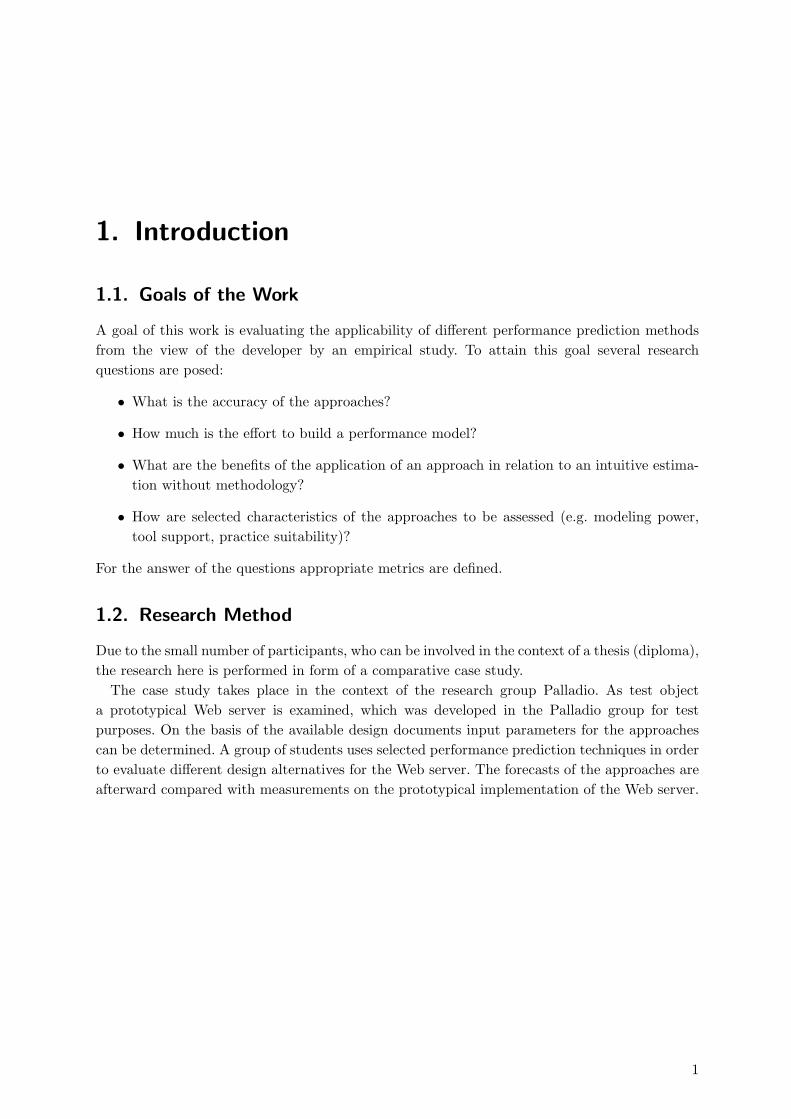
1.1. Goals of the Work
A goal of this work is evaluating the applicability of different performance prediction methodsfrom the view of the developer by an empirical study. To attain this goal several researchquestions are posed:
• What is the accuracy of the approaches?
• How much is the effort to build a performance model?
• What are the benefits of the application of an approach in relation to an intuitive estima-tion without methodology?
• How are selected characteristics of the approaches to be assessed (e.g. modeling power,tool support, practice suitability)?
For the answer of the questions appropriate metrics are defined.
1.2. Research Method
Due to the small number of participants, who can be involved in the context of a thesis (diploma),the research here is performed in form of a comparative case study.
The case study takes place in the context of the research group Palladio. As test objecta prototypical Web server is examined, which was developed in the Palladio group for testpurposes. On the basis of the available design documents input parameters for the approachescan be determined. A group of students uses selected performance prediction techniques in orderto evaluate different design alternatives for the Web server. The forecasts of the approaches areafterward compared with measurements on the prototypical implementation of the Web server.
1

2
2. Methodology
2.1. Research Method
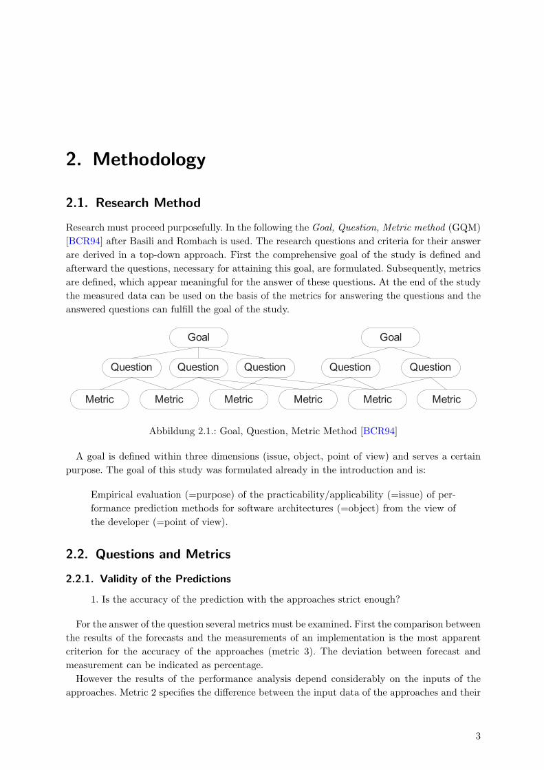
Research must proceed purposefully. In the following the Goal, Question, Metric method (GQM)[BCR94] after Basili and Rombach is used. The research questions and criteria for their answerare derived in a top-down approach. First the comprehensive goal of the study is defined andafterward the questions, necessary for attaining this goal, are formulated. Subsequently, metricsare defined, which appear meaningful for the answer of these questions. At the end of the studythe measured data can be used on the basis of the metrics for answering the questions and theanswered questions can fulfill the goal of the study.
Goal Goal
Question
Metric Metric Metric Metric Metric Metric
Question Question Question Question
Abbildung 2.1.: Goal, Question, Metric Method [BCR94]
A goal is defined within three dimensions (issue, object, point of view) and serves a certainpurpose. The goal of this study was formulated already in the introduction and is:
Empirical evaluation (=purpose) of the practicability/applicability (=issue) of per-formance prediction methods for software architectures (=object) from the view ofthe developer (=point of view).
2.2. Questions and Metrics
2.2.1. Validity of the Predictions
1. Is the accuracy of the prediction with the approaches strict enough?
For the answer of the question several metrics must be examined. First the comparison betweenthe results of the forecasts and the measurements of an implementation is the most apparentcriterion for the accuracy of the approaches (metric 3). The deviation between forecast andmeasurement can be indicated as percentage.
However the results of the performance analysis depend considerably on the inputs of theapproaches. Metric 2 specifies the difference between the input data of the approaches and their
3

2. Methodology
output data. Due to the heterogeneity of input and output data their difference can only withdifficulty be expressed in numbers and is therefore indicated on a rough scale (highly, means,low).
Input data for the approaches can be obtained in different way. In an experiment with severalparticipants can be examined, how strongly the input data of different participants differ fromeach other, if these are determined by them due to same basic informations (metric 1).
The authors of the approaches for the early performance analysis often stress that it is not theobjective of the approaches to predict exact absolute performance values. Rather the evaluationof different design alternatives is the center of attention. Therefore several design alternatives ofthe test object must be examined in the study and the participants must be asked for favoringone of the alternatives. The performance of the alternatives must then also be measured onan implementation. Afterward, it can be proportionally indicated how many participants havefavored the best design alternative concerning the performance (metric 4). If the forecasts ofthe participants are so inaccurate that in each case different alternatives are selected then theapproaches would be useless for normal developers and performance experts would have to beconsulted.
The metrics for the answer to first question are summarised in table 2.1. This table is usedalso later for the evaluation.
Difference ininput andoutput dataof differentparticipant
Difference ininput andoutput data
Difference ininput data andmeasurements
percentage ofcorrect designdecisions
(metric 1) (metric 2) (metric 3) (metric 4)approach 1approach 2. . .approach n
Tabelle 2.1.: Validity of prediction
2.2.2. Effort/Costs for the Performance Prediction
An argument of practitioners to neglect performance analysis during the design process is stillthe high investment of time, which the application of these techniques require. The secondquestion is therefore to examine this circumstances more near and is:
2. What is the effort for the performance prediction?
Performance prediction methods are deployed in practice only if the expenditure of the costsis justified. A comparison of the costs for the performance analysis with the saved time byadditional changes of design is not possible in the context of this case study. Nevertheless atleast the learning expenditure for the approaches (metric 5) and the time for the transformationof a design specification into a performance model (metric 6) can be measured.
4
2.2. Questions and Metrics
2.2.3. Methodical in relation to Intuitive Manner
3. What are the advantages of applying of performance prediction techniques inrelation to an intuitive manner?
In the study an untrained control group gets the same tasks as the participants, who applythe performance prediction approaches. The recommendations for the best design alternativesby the control group are compared with the recommended alternatives, which were obtainedwith application of the approaches (metric 7).
2.2.4. Evaluation of Individual Characteristics
The quality and the degree of mature of the approaches is examined with a further question:
4. How are selected characteristics of the performance analysis methods to be asses-sed?
This general question can be answered by means of a set of concrete criteria. The followingcriterion pattern was developed (metric 8, partly following [?]):
• Notation, used software and performance models
– Power (Which constructs can be specified, which not?)
– Structuring (Are the representations understandable? Is there a modularity of theperformance model?)
– Specification of performance values (In which form estimations or measurements getinto the performance model?)
• Tool support
– User interface, ergonomics (How user-friendly are the tools?)
– Robustness related to incorrect inputs (How robust are the tools in relation to usageerrors?)
– Presentation of the results (Is the comprehensibleness for the developer ensured?)
– practice suitability (Are the software tools sophisticated for application in the softwareindustry?)
• Suitability for different domains
• Evaluation method (which methods are used, which are the assets and drawbacks?)
• Process integration (Is there a process model, what is the degree of integration into thesoftware development process?)
2.2.5. Summary
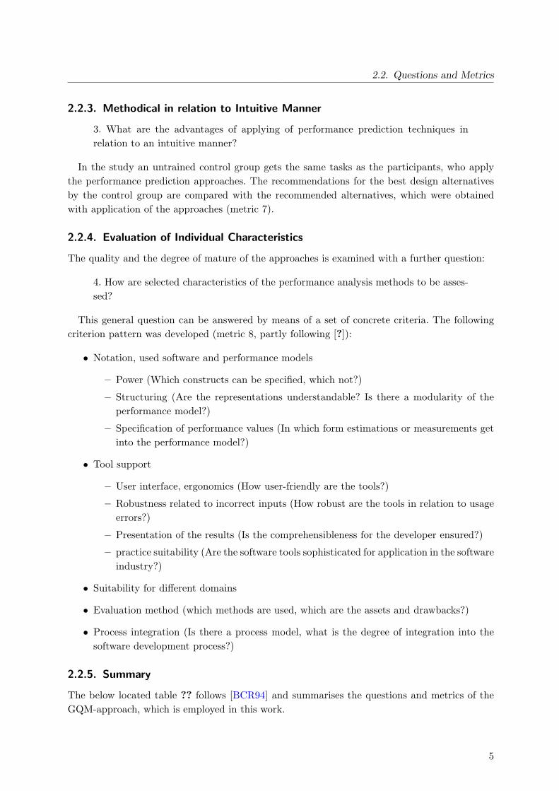
The below located table ?? follows [BCR94] and summarises the questions and metrics of theGQM-approach, which is employed in this work.
5
2. Methodology
Goal Purpose Empirical EvaluationIssue of applianceObject of performance prediction approachesPoint ofview
from the view of the developer. Scale
Question F1 What is the accuracy of the prediction with the ap-proaches?
Metric M1 Deviation of input data of different participants secondsM2 Deviation of input and output data low, mean,
highM3 Deviation of output data and measurements percentageM4 Percentage of correct predicted design alternatives percentage
Question F2 What is the effort for the performance prediction?Metric M5 Learning expenditure hours
M6 Duration of performance modeling hours
Question F3 What advantages have performance evaluation tech-niques over the intuitive way?
Metric M7 Deviation of percentage of correct predicted design de-cisions
percentage
Question F4 How are selected characteristics of the performanceanalysis methods to be assessed?
Metric M8 Criterion schema
Tabelle 2.2.: Summary GQM
6
3. Concept and Realisation of the Case Study
The core of this case study is the experimental study of an prototypical Web server with threeselected performance analysis approaches (SPE, umlPSI, Capacity Planning).
3.1. Boundary Conditions
The participants of the case study were 24 students of the lecture ”Component based softwaredevelopment“ at the University of Oldenburg in the summer term 2004. The participants weredistributed into 3 groups of 8 persons.
The participants had two hours to examine one of the software-architectures of a web serverwith varying input parameters for the approaches. Additionally they evaluated with the help ofthe performance prediction approaches five different design alternatives for the Web server inrespect of their performance behavior. Details about the experiment can be found in section 3.2.
To have a reference group, seven further participants took part in the experiment withoutknowing the performance-analysis approaches. Their recommendation are given in section 4.2.
All design-alternatives have been implemented for the web server. Using this implementationsit was possible to evaluate the predictions of the performance-approaches. The results can befound in section 4.1.4.
3.2. Experiment
3.2.1. Webserver-Architecture
The experiment focused on a experimental web server, which was developed in the palladio-group. The first version of the implementation was done in a completely object-oriented way,based on the .NET-Framework under Microsoft Visual Studio. Within a student work the serverhad been transformed to a component based web server. This includes the introduction ofremovable components and interfaces to connect to external applications and databases. So theweb server could be used as a component based example system.
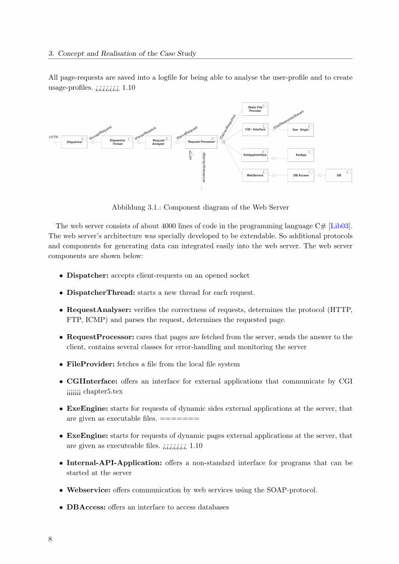
¡¡¡¡¡¡¡ chapter5.tex The server accepts client-request by the HTTP-protocol and delivers therequested web pages (e. g. HTML- or image-files). It is constructed multi-threaded, so that foreach request a own program-thread is created to be able to handle multiple parallel requests.HTML-files can be created dynamically as well, e. g. to include user-dependent information. Allpage-requests are saved into a log file for being able to analyse the user-profile and to createusage-profiles. ======= The server accepts client-request by the HTTP-protocol and deliver-es the requested pages (e. g. HTML- or image-files). It is constructed multi-threaded, so that foreach request a own programm-thread is created to be able to handle multiple parallel requests.HTML-files can be created dynamically as well, e. g. to include user-dependant information.
7
3. Concept and Realisation of the Case Study
All page-requests are saved into a logfile for being able to analyse the user-profile and to createusage-profiles. ¿¿¿¿¿¿¿ 1.10
Dispatcher DispatcherThread
Request ProcessorRequest Analyzer
Static File Provider
CGI - Interface
ExtAppInterface
WebService DB Access DB
Exe - Engin
HTTP IAccep
tReque
st
IParse
Reques
t
IServe
Reque
st
HTT
P IMonitorW
ebserver
IDeliverResponse
IGetRe
sponse
Stream
ExtApp
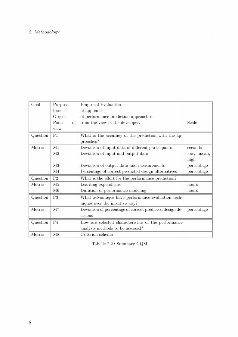
Abbildung 3.1.: Component diagram of the Web Server
The web server consists of about 4000 lines of code in the programming language C# [Lib03].The web server’s architecture was specially developed to be extendable. So additional protocolsand components for generating data can integrated easily into the web server. The web servercomponents are shown below:
• Dispatcher: accepts client-requests on an opened socket
• DispatcherThread: starts a new thread for each request.
• RequestAnalyser: verifies the correctness of requests, determines the protocol (HTTP,FTP, ICMP) and parses the request, determines the requested page.
• RequestProcessor: cares that pages are fetched from the server, sends the answer to theclient, contains several classes for error-handling and monitoring the server
• FileProvider: fetches a file from the local file system
• CGIInterface: offers an interface for external applications that communicate by CGI¡¡¡¡¡¡¡ chapter5.tex
• ExeEngine: starts for requests of dynamic sides external applications at the server, thatare given as executable files. =======
• ExeEngine: starts for requests of dynamic pages external applications at the server, thatare given as executeable files. ¿¿¿¿¿¿¿ 1.10
• Internal-API-Application: offers a non-standard interface for programs that can bestarted at the server
• Webservice: offers communication by web services using the SOAP-protocol.
• DBAccess: offers an interface to access databases
8
3.2. Experiment
Requests from the RequestProcessor are passed to further components by the IDeliverResponse-interface. This components are organized according to the ”Chain of Responsibility“ design-pattern [GHJV95]. The results of the performance-analysis of the implementation can be foundin chapter 4.1.4.
3.2.2. Task
For the experiment a task had to be found, that could give answers to the research questions fromchapter 2. As a typical use-case for performance-analysis-approaches the evaluation of design-decisions should be focused. The absolute performance measuring using the web server wouldhave been possible with the examined approach, but in this experiment the participants didnot have the implementation, as the performance-analysis for early stages of the design-processshould be examined.
The task orientated on the given design-documents of the web server. For each design-alternative a UML-component-diagram war given. This diagram had to be prepared to be of usefor the experiment. The diagrams should be usable as direct input parameters for the approa-ches, because the participants of the experiment should do as little routine work as possible.The following artefacts had been created:
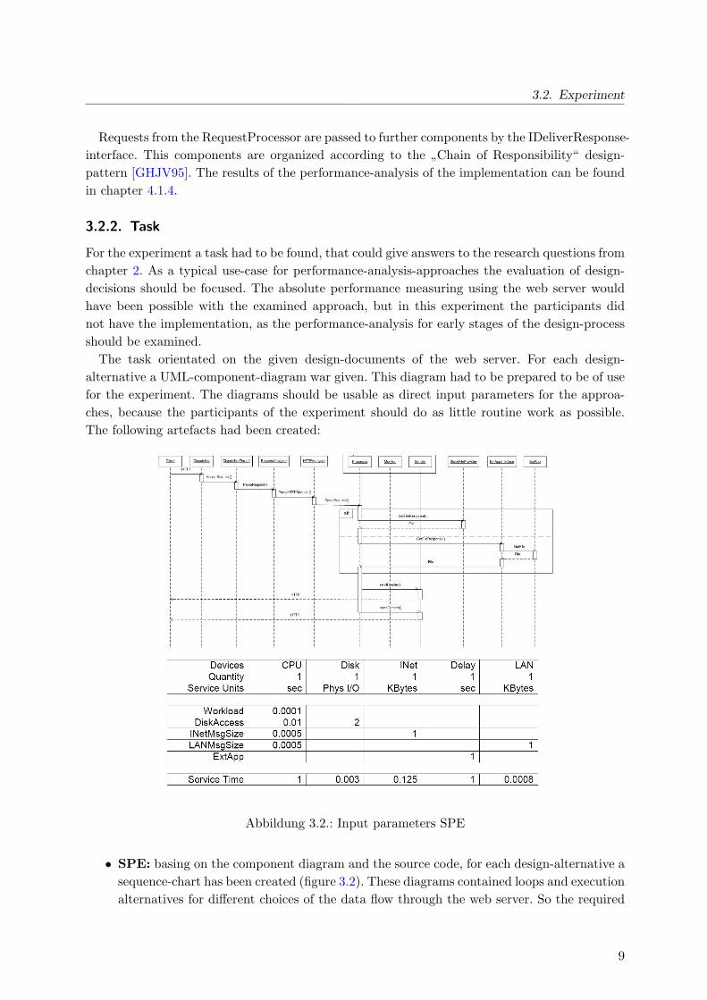
Abbildung 3.2.: Input parameters SPE
• SPE: basing on the component diagram and the source code, for each design-alternative asequence-chart has been created (figure 3.2). These diagrams contained loops and executionalternatives for different choices of the data flow through the web server. So the required
9
3. Concept and Realisation of the Case Study
execution graphs could be easily created with the SPE-ED-tool. The ”software-resources“were given. The ”processing-overhead“ (a table in which the requirements of the software-resources were depicted to the hardware-resources) was given as well. The preset of thesevalues is usual in practice, as the values are given by performance-experts. The valueswere determined by measuring different kinds of network-connections and by using typicalvalues for e. g. ISDN-connections to the client or 10 MBit-connections between the webserver and an external server. This hardware-settings were simulated for later performancemeasuring with the web server. Additionally a queuing-model for distributing resourceswas given, which in fact was simply illustrating the settings, but could not be used withthe SPE-ED-tool.
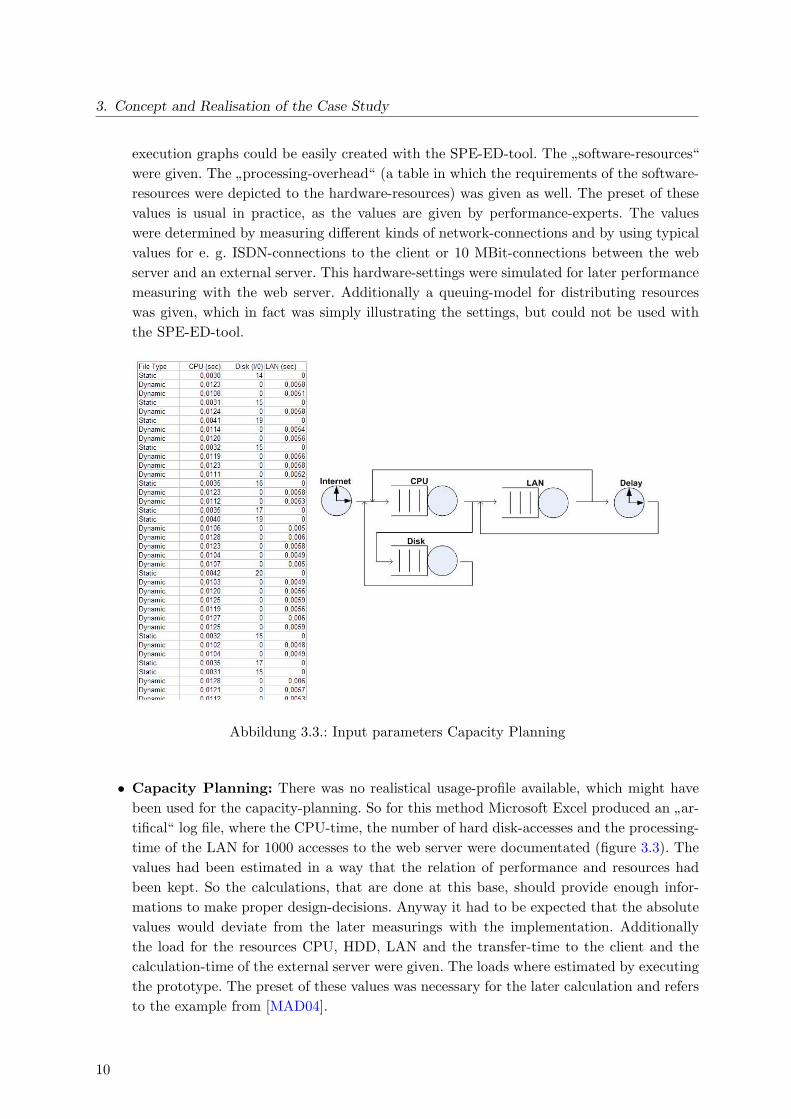
Abbildung 3.3.: Input parameters Capacity Planning
• Capacity Planning: There was no realistical usage-profile available, which might havebeen used for the capacity-planning. So for this method Microsoft Excel produced an ”ar-tifical“ log file, where the CPU-time, the number of hard disk-accesses and the processing-time of the LAN for 1000 accesses to the web server were documentated (figure 3.3). Thevalues had been estimated in a way that the relation of performance and resources hadbeen kept. So the calculations, that are done at this base, should provide enough infor-mations to make proper design-decisions. Anyway it had to be expected that the absolutevalues would deviate from the later measurings with the implementation. Additionallythe load for the resources CPU, HDD, LAN and the transfer-time to the client and thecalculation-time of the external server were given. The loads where estimated by executingthe prototype. The preset of these values was necessary for the later calculation and refersto the example from [MAD04].
10
3.2. Experiment
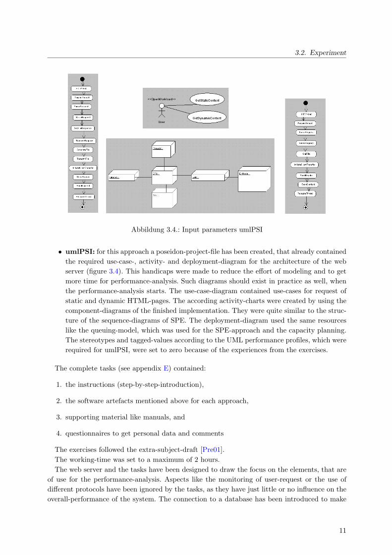
Abbildung 3.4.: Input parameters umlPSI
• umlPSI: for this approach a poseidon-project-file has been created, that already containedthe required use-case-, activity- and deployment-diagram for the architecture of the webserver (figure 3.4). This handicaps were made to reduce the effort of modeling and to getmore time for performance-analysis. Such diagrams should exist in practice as well, whenthe performance-analysis starts. The use-case-diagram contained use-cases for request ofstatic and dynamic HTML-pages. The according activity-charts were created by using thecomponent-diagrams of the finished implementation. They were quite similar to the struc-ture of the sequence-diagrams of SPE. The deployment-diagram used the same resourceslike the queuing-model, which was used for the SPE-approach and the capacity planning.The stereotypes and tagged-values according to the UML performance profiles, which wererequired for umlPSI, were set to zero because of the experiences from the exercises.
The complete tasks (see appendix E) contained:
1. the instructions (step-by-step-introduction),
2. the software artefacts mentioned above for each approach,
3. supporting material like manuals, and
4. questionnaires to get personal data and comments
The exercises followed the extra-subject-draft [Pre01].The working-time was set to a maximum of 2 hours.The web server and the tasks have been designed to draw the focus on the elements, that are
of use for the performance-analysis. Aspects like the monitoring of user-request or the use ofdifferent protocols have been ignored by the tasks, as they have just little or no influence on theoverall-performance of the system. The connection to a database has been introduced to make
11
3. Concept and Realisation of the Case Study
the performance-analysis more complex and less obviously. The two-tier architecture of the webserver with the database on a separate server is quite easily but usual in practice. For the tasksthe number of threads and the size of the used files were given, because this aspect probablywould have had a big influence to the performance.
The tasks for the experiment had to be designed in a way, that none of the examined approa-ches could take advantages. In this study none of the three approaches should be disadvantaged,because the input parameters had been customized for each process.
3.2.3. Design-alternatives
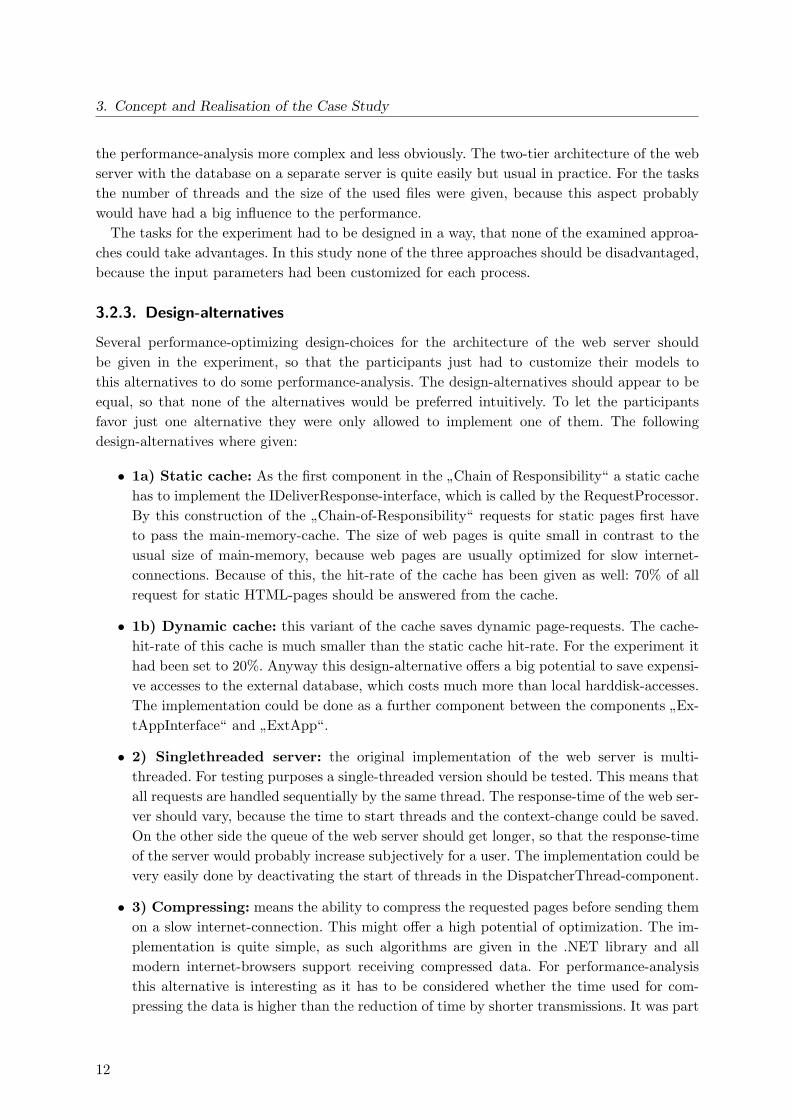
Several performance-optimizing design-choices for the architecture of the web server shouldbe given in the experiment, so that the participants just had to customize their models tothis alternatives to do some performance-analysis. The design-alternatives should appear to beequal, so that none of the alternatives would be preferred intuitively. To let the participantsfavor just one alternative they were only allowed to implement one of them. The followingdesign-alternatives where given:
• 1a) Static cache: As the first component in the ”Chain of Responsibility“ a static cachehas to implement the IDeliverResponse-interface, which is called by the RequestProcessor.By this construction of the ”Chain-of-Responsibility“ requests for static pages first haveto pass the main-memory-cache. The size of web pages is quite small in contrast to theusual size of main-memory, because web pages are usually optimized for slow internet-connections. Because of this, the hit-rate of the cache has been given as well: 70% of allrequest for static HTML-pages should be answered from the cache.
• 1b) Dynamic cache: this variant of the cache saves dynamic page-requests. The cache-hit-rate of this cache is much smaller than the static cache hit-rate. For the experiment ithad been set to 20%. Anyway this design-alternative offers a big potential to save expensi-ve accesses to the external database, which costs much more than local harddisk-accesses.The implementation could be done as a further component between the components ”Ex-tAppInterface“ and ”ExtApp“.
• 2) Singlethreaded server: the original implementation of the web server is multi-threaded. For testing purposes a single-threaded version should be tested. This means thatall requests are handled sequentially by the same thread. The response-time of the web ser-ver should vary, because the time to start threads and the context-change could be saved.On the other side the queue of the web server should get longer, so that the response-timeof the server would probably increase subjectively for a user. The implementation could bevery easily done by deactivating the start of threads in the DispatcherThread-component.
• 3) Compressing: means the ability to compress the requested pages before sending themon a slow internet-connection. This might offer a high potential of optimization. The im-plementation is quite simple, as such algorithms are given in the .NET library and allmodern internet-browsers support receiving compressed data. For performance-analysisthis alternative is interesting as it has to be considered whether the time used for com-pressing the data is higher than the reduction of time by shorter transmissions. It was part
12
3.3. Performance Analysis of the Implementation
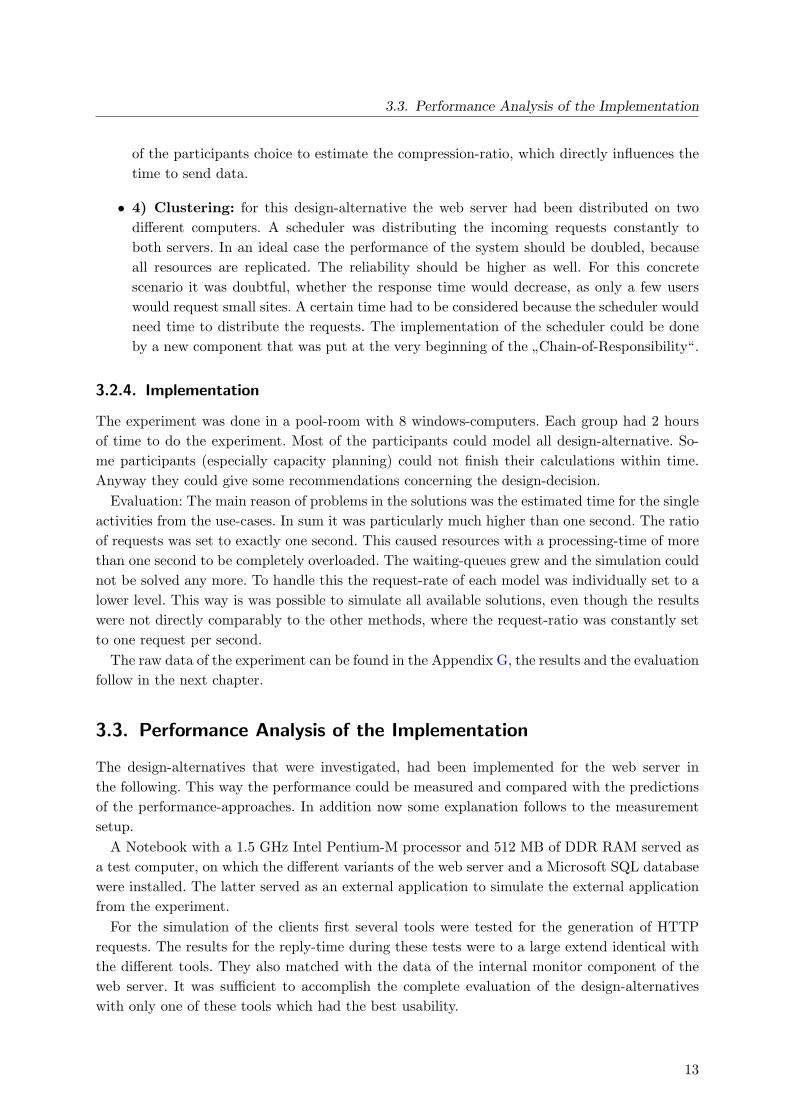
of the participants choice to estimate the compression-ratio, which directly influences thetime to send data.
• 4) Clustering: for this design-alternative the web server had been distributed on twodifferent computers. A scheduler was distributing the incoming requests constantly toboth servers. In an ideal case the performance of the system should be doubled, becauseall resources are replicated. The reliability should be higher as well. For this concretescenario it was doubtful, whether the response time would decrease, as only a few userswould request small sites. A certain time had to be considered because the scheduler wouldneed time to distribute the requests. The implementation of the scheduler could be doneby a new component that was put at the very beginning of the ”Chain-of-Responsibility“.
3.2.4. Implementation
The experiment was done in a pool-room with 8 windows-computers. Each group had 2 hoursof time to do the experiment. Most of the participants could model all design-alternative. So-me participants (especially capacity planning) could not finish their calculations within time.Anyway they could give some recommendations concerning the design-decision.
Evaluation: The main reason of problems in the solutions was the estimated time for the singleactivities from the use-cases. In sum it was particularly much higher than one second. The ratioof requests was set to exactly one second. This caused resources with a processing-time of morethan one second to be completely overloaded. The waiting-queues grew and the simulation couldnot be solved any more. To handle this the request-rate of each model was individually set to alower level. This way is was possible to simulate all available solutions, even though the resultswere not directly comparably to the other methods, where the request-ratio was constantly setto one request per second.
The raw data of the experiment can be found in the Appendix G, the results and the evaluationfollow in the next chapter.
3.3. Performance Analysis of the Implementation
The design-alternatives that were investigated, had been implemented for the web server inthe following. This way the performance could be measured and compared with the predictionsof the performance-approaches. In addition now some explanation follows to the measurementsetup.
A Notebook with a 1.5 GHz Intel Pentium-M processor and 512 MB of DDR RAM served asa test computer, on which the different variants of the web server and a Microsoft SQL databasewere installed. The latter served as an external application to simulate the external applicationfrom the experiment.
For the simulation of the clients first several tools were tested for the generation of HTTPrequests. The results for the reply-time during these tests were to a large extend identical withthe different tools. They also matched with the data of the internal monitor component of theweb server. It was sufficient to accomplish the complete evaluation of the design-alternativeswith only one of these tools which had the best usability.
13
3. Concept and Realisation of the Case Study
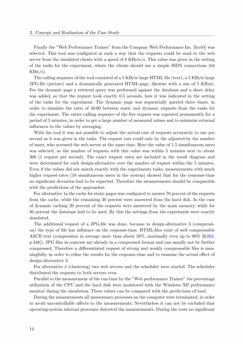
Finally the ”Web Performance Trainer” from the Company Web Performance Inc. [Inc04] wasselected. This tool was configured in such a way that the requests could be send to the webserver from the simulated clients with a speed of 8 KByte/s. This value was given in the settingof the tasks for the experiment, where the clients should use a simple ISDN connections (64KBit/s).
The calling sequence of the tool consisted of a 5 KByte large HTML file (text), a 5 KByte largeJPG-file (picture) and a dynamically generated HTML-page, likewise with a size of 5 KByte.For the dynamic page a retrieval query was performed against the database and a short delaywas added, so that the request took exactly 0.5 seconds, how it was indicated in the settingof the tasks for the experiment. The dynamic page was sequentially queried three times, inorder to simulate the ratio of 40:60 between static and dynamic requests from the tasks forthe experiment. The entire calling sequence of the five request was repeated permanently for aperiod of 5 minutes, in order to get a large number of measured values and to minimize externalinfluences to the values by averaging.
With the tool it was not possible to adjust the arrival rate of requests accurately to one persecond as it was given in the tasks. The request rate could only by the adjusted by the numberof users, who accessed the web server at the same time. Here the value of 1.5 simultaneous userswas selected, as the number of requests with this value was within 5 minutes next to about300 (1 request per second). The exact request rates are included in the result diagram andwere determined for each design-alternative over the number of request within the 5 minutes.Even if the values did not match exactly with the experiments tasks, measurements with muchhigher request-rates (10 simultaneous users in the system) showed that for the response-timeno significant deviation had to be expected. Therefore the measurements should be comparablewith the predictions of the approaches.
For alternative 1a the cache for static pages was configured to answer 70 percent of the requestsfrom the cache, while the remaining 30 percent were answered from the hard disk. In the caseof dynamic caching 20 percent of the requests were answered by the main memory, while for80 percent the database had to be used. By this the settings from the experiment were exactlysimulated.
The additional request of a JPG-file was done, because in design-alternative 3 (compressi-on) the type of file has influence on the response-time. HTML-files exist of well compressableASCII text (compression in average more than about 50%, maximally even up to 90% [Kil02,p.348]). JPG files in contrast are already in a compressed format and can usually not be furthercompressed. Therefore a differentiated request of strong and weakly compressable files is mea-ningfully, in order to refine the results for the response-time and to examine the actual effect ofdesign-alternative 3.
For alternative 4 (clustering) two web servers and the scheduler were started. The schedulerdistributed the requests to both servers even.
Parallel to the measurement of the run-time by the ”Web performance Trainer” the percentageutilization of the CPU and the hard disk were monitored with the Windows XP performancemonitor during the simulation. These values can be compared with the predictions of load.
During the measurements all unnecessary processes on the computer were terminated, in orderto avoid uncontrollable affects to the measurements. Nevertheless it can not be excluded thatoperating-system internal processes distorted the measurements. During the tests no significant
14
3.3. Performance Analysis of the Implementation
events occured. The measurement took 5 minutes. The average response-times was calculatedfor each case. The raw data of all measurements can be found in the appendix I, diagrams withthe average values follow in section 4.1.4.
15

16
4. Results
In chapter 2 4 questions about performance evaluation approaches were posed. In this chapterthe collected data are illustrated and interpreted in respect of this questions.
4.1. Validity of the prediction
1. What is the accuracy of the forecasting with the performance prediction approa-ches?
In order to come up to this question, four metrics were specified: the deviation in the inputdata of different participants (metric 1), the discrepancy in the input and output data of dif-ferent approaches (metric 2), the discrepancy of output data of the approaches in relation tomeasurements (metric 3) and the percentage of proper design decisions (metric 4).
As with the approaches equal input data are mapped to identical outputs it is sufficient toconsider the output data in order to analyse metric 1.
During the experiment response time and throughput(utilisation) were predicted with thethree approaches.
4.1.1. Predictions with SPE
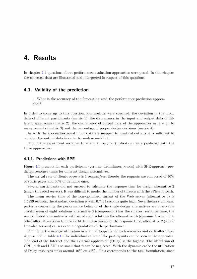
Figure 4.1 presents for each participant (german: Teilnehmer, x-axis) with SPE-approach pre-dicted response times for different design alternatives.
The arrival rate of client-requests is 1 request/sec, thereby the requests are composed of 40%of static pages and 60% of dynamic ones.
Several participants did not succeed to calculate the response time for design alternative 2(single threaded servers). It was difficult to model the number of threads with the SPE-approach.
The mean service time of the non-optimised variant of the Web server (alternative 0) is1.5999 seconds, the standard deviation is with 0.7431 seconds quite high. Nevertheless significantpatterns concerning the performance behavior of the single design alternatives are observable. With seven of eight solutions alternative 3 (compression) has the smallest response time, thesecond fastest alternative is with six of eight solutions the alternative 1b (dynamic Cache). Theother alternatives seem to provide little improvements of the response time, alternative 2 (singlethreaded servers) causes even a degradation of the performance.
For clarity the average utilization over all participants for each resources and each alternativeis presented in table 4.1. The individual values of the participants can be seen in the appendix.The load of the Internet and the external application (Delay) is the highest. The utilization ofCPU, disk and LAN is so small that it can be neglected. With the dynamic cache the utilizationof Delay resources sinks around 10% on 42% . This corresponds to the task formulation, since
17
4. Results
0,0
0,5
1,0
1,5
2,0
2,5
3,0
3,5
Teilnehmer
Dur
chla
ufze
it in
Sek
unde
n
Alternative 0 1,1928 2,9415 0,9562 1,3168 1,5503 1,8476 2,3094 0,6845
Alternative 1a 1,1883 2,9338 0,9499 1,3108 1,5196 1,8204 2,3030 0,6200
Alternative 1b 1,1317 2,8670 0,8981 1,2545 1,4868 1,7826 2,1478 0,5800
Alternative 2 0,9546 1,3482 1,5477 1,8428 2,3944
Alternative 3 0,8188 1,6856 0,7096 0,8766 1,2979 1,1221 1,8822 0,6089
Alternative 4 1,1952 2,9367 0,9588 1,3152 1,5323 1,8421 1,9892 0,6878
1 2 3 4 5 6 7 8
Abbildung 4.1.: Predicted response times with SPE-approach
CPU Disk LAN Delay InetAlternative 0: no optimisation 5% 2% 0% 53% 125%Alternative 1a: statical cache 4% 2% 0% 52% 125%Alternative 1b: dynamical cache 4% 3% 0% 42% 124%Alternative 2: single-threaded Server 8% 4% 0% 102% 178%Alternative 3: compressing 5% 3% 0% 48% 78%Alternative 4: clustering 3% 1% 0% 48% 125%
Tabelle 4.1.: Predicted utilization with SPE-approach (mean)
18
4.1. Validity of the prediction
the data now can be accessed directly from the main storage of the Web server and the externalapplication is addressed more rarely.
4.1.2. Prediction with Capacity Planning
0,00,20,40,60,81,01,21,41,61,82,0
Teilnehmer
Dur
chla
ufze
it in
Sek
unde
n
Alternative 0 1,50536 1,50536 1,50533 1,50524 1,50510 1,50522
Alternative 1a 1,50536 1,50536 1,50533 1,50524 1,50510 1,50522
Alternative 1b 1,40399 1,40399 1,40397 1,40387 1,40373 1,40386
Alternative 2 1,49110 1,49190
Alternative 3 1,21125 1,26893 1,18273 1,40061 1,98167 1,10916
Alternative 4 1,45336 1,45336 1,44094 1,44089 1,44082 1,44089
1 2 3 4 5 6
Abbildung 4.2.: Predicted response times with CP-approach (dynamical site requests)
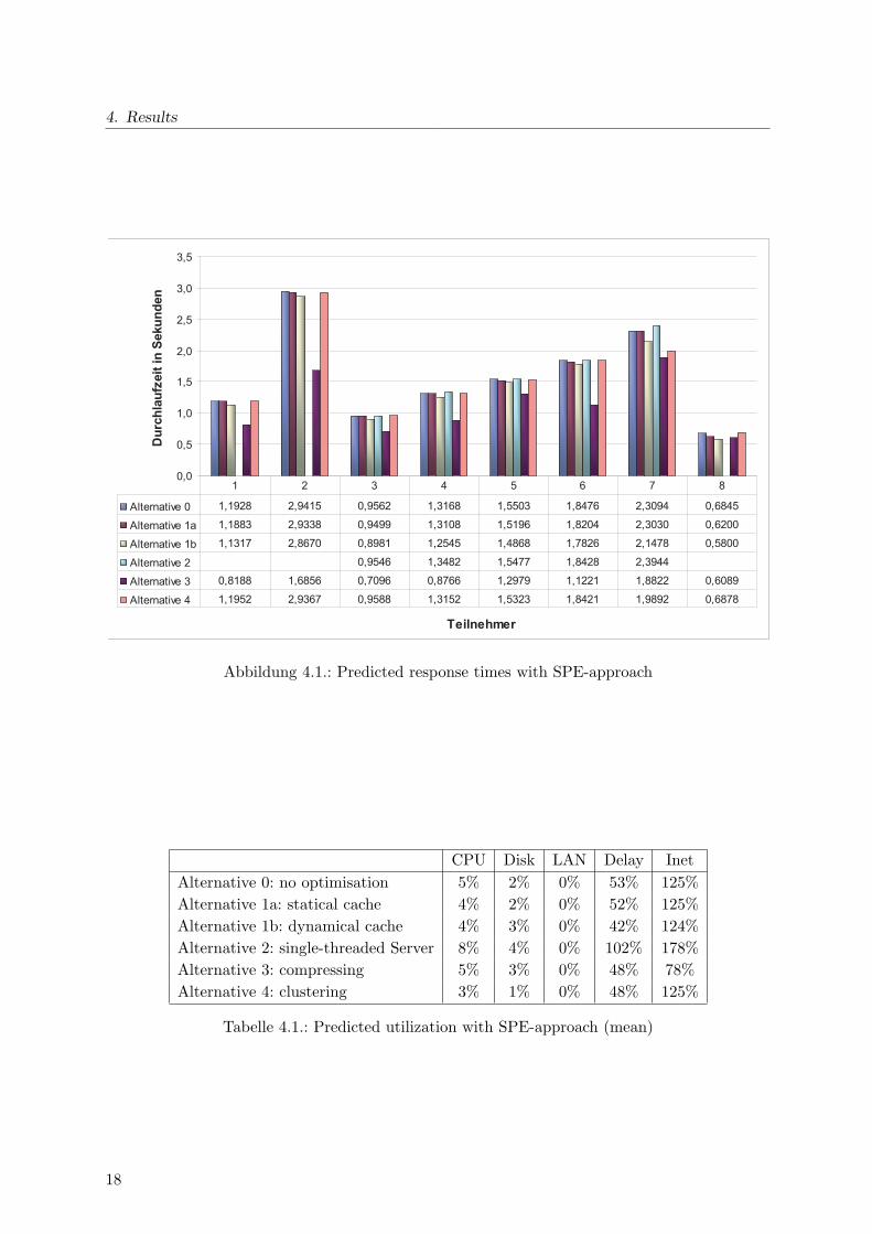
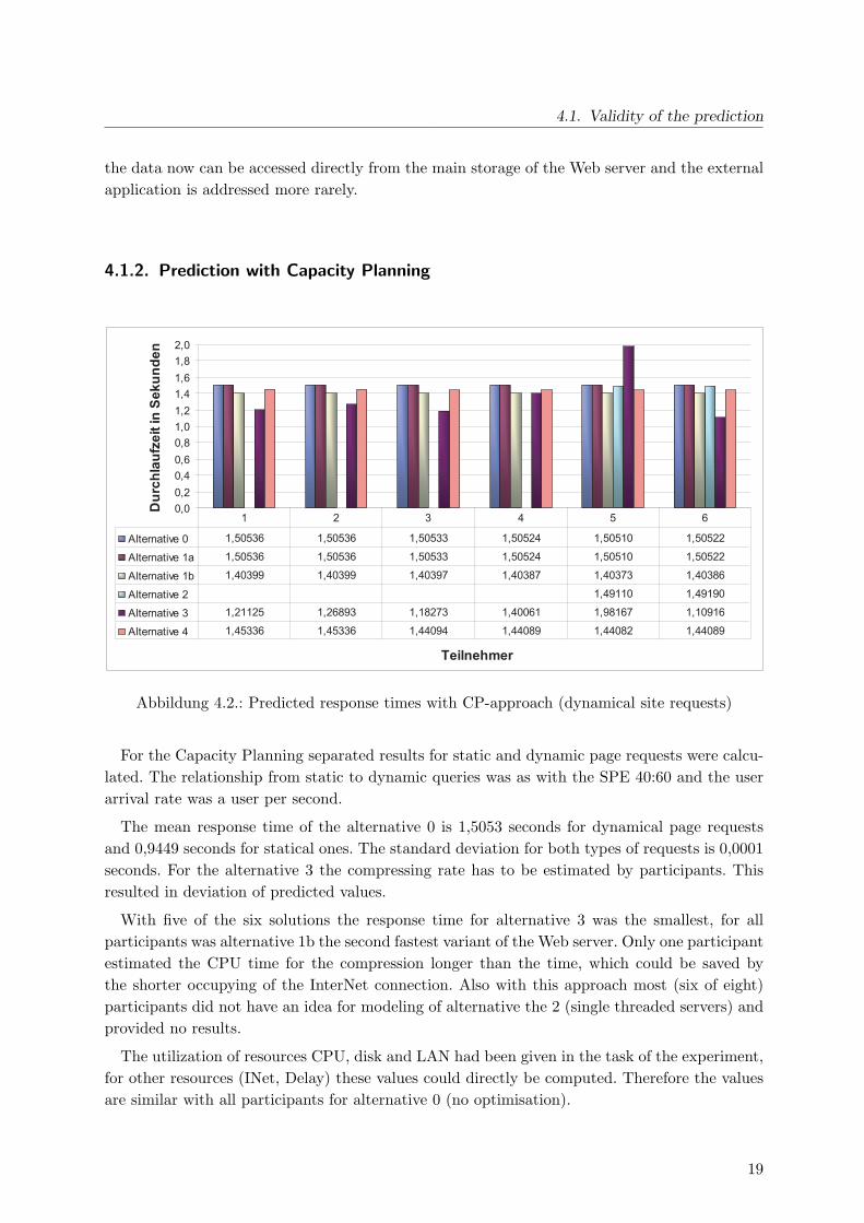
For the Capacity Planning separated results for static and dynamic page requests were calcu-lated. The relationship from static to dynamic queries was as with the SPE 40:60 and the userarrival rate was a user per second.
The mean response time of the alternative 0 is 1,5053 seconds for dynamical page requestsand 0,9449 seconds for statical ones. The standard deviation for both types of requests is 0,0001seconds. For the alternative 3 the compressing rate has to be estimated by participants. Thisresulted in deviation of predicted values.
With five of the six solutions the response time for alternative 3 was the smallest, for allparticipants was alternative 1b the second fastest variant of the Web server. Only one participantestimated the CPU time for the compression longer than the time, which could be saved bythe shorter occupying of the InterNet connection. Also with this approach most (six of eight)participants did not have an idea for modeling of alternative the 2 (single threaded servers) andprovided no results.
The utilization of resources CPU, disk and LAN had been given in the task of the experiment,for other resources (INet, Delay) these values could directly be computed. Therefore the valuesare similar with all participants for alternative 0 (no optimisation).
19
4. Results
0,00,10,20,30,40,50,60,70,80,91,0
Teilnehmer
Dur
chla
ufze
it in
Sek
unde
n
Alternative 0 0,94486 0,94486 0,94489 0,94485 0,94506 0,94464
Alternative 1a 0,92410 0,92410 0,92413 0,92423 0,92424 0,92395
Alternative 1b 0,94486 0,94486 0,94489 0,94485 0,94506 0,94464
Alternative 2 0,93770 0,94329
Alternative 3 0,51495 0,69929 0,60383 0,79294 0,86023 0,52064
Alternative 4 0,91304 0,91304 0,90899 0,90897 0,90907 0,90888
1 2 3 4 5 6
Abbildung 4.3.: Predicted response times with CP-approach (statical site requests)
CPU Disk LAN Delay InetAlternative 0: no optimisation 8,2% 1,2% 0,4% 29,5% 87,5%Alternative 1a: statical cache 8,2% 0,36% 0,4% 29,5% 87,5%Alternative 1b: dynamical cache 8,2% 1,2% 0,3% 23,6% 87,5%Alternative 2: single-threaded server 7,92% 1,2% 0,4% 29,5% 87,5%Alternative 3: compressing 15,63% 1,1% 0,4% 28,8% 48,5%Alternative 4: clustering 4,4% 0,6% 0,4% 29,5% 87,5%
Tabelle 4.2.: Predicted throughputs with CP-approach (mean)
20

4.1. Validity of the prediction
0,0
5,0
10,0
15,0
20,0
25,0
Teilnehmer
Dur
chla
ufze
it in
Sek
unde
n
Alternative 0 2,3932 5,4211 10,5690 12,2504 21,1166 6,3678 16,0072 8,7612
Alternative 1a 2,3922 5,6192 10,5812 11,6949 21,4039 5,9798 14,3145 8,6219
Alternative 1b 2,1750 5,2493 9,7972 10,4271 20,7919 5,9458 13,3239 7,1867
Alternative 2 3,2306 6,0873
Alternative 3 1,4886 3,1577 8,3245 5,2539 22,2858 5,7347 7,4177 9,3413
Alternative 4 2,3103 5,0517 9,4992 10,4794 15,3719 5,1540 16,0813 8,2451
1 2 3 4 5 6 7 8
0,5 Anfr/sec 0,5 Anfr/sec 0,2 Anfr/sec 0,17 Anfr/sec 0,06 Anfr/sec 0,2 Anfr/sec 0,2 Anfr/sec 0,17 Anfr/sec
Abbildung 4.4.: Predicted Response times with umlPSI-approach (dynamical)
0,0
5,0
10,0
15,0
20,0
Teilnehmer
Dur
chla
ufze
it in
Sek
unde
n
Alternative 0 1,6542 4,8946 8,5177 9,5530 16,5900 3,9858 14,8026 3,7014
Alternative 1a 1,6285 4,8108 7,8333 8,3332 16,2966 3,7857 11,5626 3,6322
Alternative 1b 1,6742 4,8831 7,2854 9,7705 16,0725 3,6201 11,7189 3,6938
Alternative 2 2,5957 3,8117
Alternative 3 0,8839 2,6538 7,3874 5,2539 17,3815 3,4865 5,9705 4,4117
Alternative 4 1,5086 4,3526 7,1448 10,4794 10,9589 2,8569 11,8371 3,2515
1 2 3 4 5 6 7 8
0,5 Anfr/sec 0,5 Anfr/sec 0,2 Anfr/sec 0,17 Anfr/sec 0,06 Anfr/sec 0,2 Anfr/sec 0,2 Anfr/sec 0,17 Anfr/sec
Abbildung 4.5.: Predicted Response times with umlPSI-approach (statical)
21

4. Results
4.1.3. Prediction with umlPSI-approach
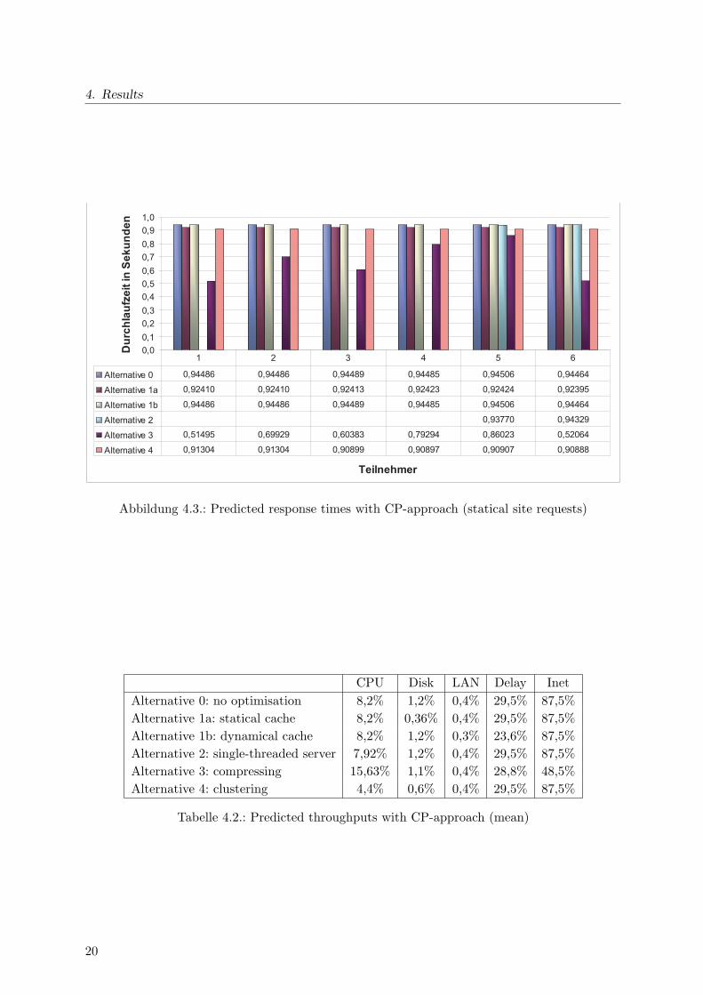
The umlPSI-approach provides also separate performance-results for statical and dynamical pagerequests in relation 40:60. For the simulation of the performance models another arrival rate forthe incoming requests had to be given than with the other approaches (there it was a query persecond). Otherwise the simulator routine due to the high estimations for the input data wouldbe overloaded. The arrival rate for requests was therefore adapted individually in each case foreach participant, so that the simulation was not overloaded. Therefore the response times andutilization predicted with this approach are only conditionally comparable with those of theother approaches.
For the non-optimised version of the web server (alternative 0) the predicted mean responsetime is 10,3608 seconds for dynamical page requests and 7,9624 for statical ones. The standarddeviation is 6,0659 (dynamic) and 5,4411 (static).
All participants were able to model the alternative 2 (single threaded servers). Therefor on-ly the appropriate entry of a parameter in resources ’ ’ Threads ” was required. During thesimulation of the models with umlPSI it turned out however that in most cases no responsetime for this design alternative could be determined. Reason for it was the strong overloadingof resources ’ ’ Threads ”, which can be observe in table ?? for utilization, where this resourcesare utilised with 100 percent (alternative 2).
CPU Disk LAN Delay Inet ThreadsAlternative 0: no optimisation 19,3% 4,0% 10,0% 9,4% 52,2% 25,8%Alternative 1a: statical Cache 19,6% 1,4% 10,2% 9,4% 52,0% 25,4%Alternative 1b: dynamical Cache 19,0% 4,0% 8,2% 7,5% 51,5% 24,4%Alternative 2: single-threaded Server 17,8% 3,6% 9,5% 8,9% 49,7% 100,0%Alternative 3: compressing 29,9% 3,9% 10,0% 9,4% 34,1% 21,6%Alternative 4: Clustering 12,0% 2,0% 10,0% 9,4% 52,0% 21,2%
Tabelle 4.3.: predicted utilisation with umlPSI-approach (mean)
4.1.4. Measurement Results of the Implementation
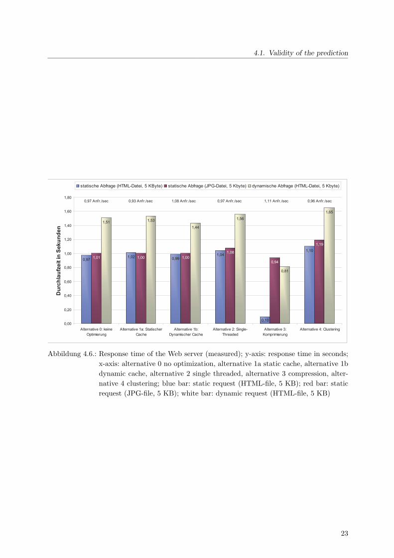
The tests setting for performance measuring of the implementation, for the different variants ofthe web server, have been discussed in section 3.3. Now the results of the measuring will follow.The average values for response time (figure 4.6) and the load (fugure 4.7) of the web server willbe presented for each variant.
For the non-optimized version of the web server the response times for both types of staticpages (HTML-document and the JPG-image from the hard disk, each with a size of 5 KByte)was nearly identically. The request of the dynamic page (HTML-document from the database,5 KByte of size) took quite exactly 0.5 seconds more of time. This fits to the settings from thetask of the experiment and can be used as a initial position.
The measuring of the variant with the static cache shows, that within the measuring precisionno deviation (at most a little rise of time) of the response time for static pages, comparedwith the non-optimized variant, could be found. This is surprising, as at least 70 percent of thestatic requests for this alternative had to be answered from the main memory, which causes no
22
4.1. Validity of the prediction
0,971,02 0,99
1,041,10
1,01 1,00 1,001,08
0,94
1,19
1,51 1,53
1,44
1,56
0,81
1,65
0,100,00
0,20
0,40
0,60
0,80
1,00
1,20
1,40
1,60
1,80
Alternative 0: keineOptimierung
Alternative 1a: StatischerCache
Alternative 1b:Dynamischer Cache
Alternative 2: Single-Threaded
Alternative 3:Komprimierung
Alternative 4: Clustering
Dur
chla
ufze
it in
Sek
unde
n
statische Abfrage (HTML-Datei, 5 KByte) statische Abfrage (JPG-Datei, 5 Kbyte) dynamische Abfrage (HTML-Datei, 5 Kbyte)
0,93 Anfr./sec0,97 Anfr./sec 0,97 Anfr./sec 1,11 Anfr./sec 0,96 Anfr./sec1,08 Anfr./sec
Abbildung 4.6.: Response time of the Web server (measured); y-axis: response time in seconds;x-axis: alternative 0 no optimization, alternative 1a static cache, alternative 1bdynamic cache, alternative 2 single threaded, alternative 3 compression, alter-native 4 clustering; blue bar: static request (HTML-file, 5 KB); red bar: staticrequest (JPG-file, 5 KB); white bar: dynamic request (HTML-file, 5 KB)
23
4. Results
expensive harddisk-access. For the more precisely investigation of this observation the WindowsXP Performance Monitor was used to measure the number of reading accesses to the harddisk ofthe non-optimized version of the server. It became clear, that from the 50 repeating requests onlythe very first caused a harddisk access at the beginning, though the static cache was deactivated.This phenomenon is caused by the operating system windows itself, which puts the called filesto a system cache in the main memory, from which the following request were answered. Sothe implementation of the static cache was useless, as the operating system did the caching. Amanual deactivation of the system cache is not performable, as this option is anchored deep insideof the operating system. For the file opening methods from the .NET-classlibrary which wereused for the implementation this cache is fully transparent. The suggested design-alternative,that used the static cache was fully irrelevant for practice. This behaviour could not be predictedby the performance-analysis-approaches.
For the use of a dynamic cache a reduction of response time of dynamic page requests wasdetermined as expected (from 1.51 seconds to 1.44 seconds). From the raw data in appendix I iscan be easily seen, that the dynamic cache was activated after about 80 percent of the requests.The response time for the following dynamic request reduced to about 1 second and correspondsto the response time of static requests that are answered from the main memory. The averagevalue of cached and non-cached requests for this alternative only reveals a little performance-winof 0.07 seconds. This value is tightly coupled to the handicap, that only 20 percent of the requestsare cached, so this values is strongly dependent on the used application. If a web-applicationallows to cache much more dynamic content, the response time would decrease, whereas thelower limit is the response time of static pages. For static pages this variant does not improvethe response time.
The single threaded server (alternative 2) shows a slightly higher response time in the com-parison to the non-optimized multi-threaded version of the web server. The requests retain andthe response time increases, as only one request can be processed at the same time by the server.With the multi-threaded version the times for the start of new Threads and the context changedo not preponderate that much, and no significant degradation of the performance results. Inthis scenario the server is loaded still too little, as maximally two request are handled at thesame time. For the examined use-case design-alternative 2 thus offers no performance advantagein comparison to the non-optimized version of the web server.
Partly very clear Performance-wins result however in the case of alternative 3 (compression).Both the static and the dynamically produced HTML-page could be well compressed, the timefor sending the files reduced proportionally to the compression factor. With the JPG file onlya slight compression is possible, here the response time only reduced about a few milliseconds.The computations, which are used for the compression, here hardly fall into weight, becausewith the compression of small files works extremely fast with the used algorithms.
With the Clustering minor performance-loss was determined, the service times increases mini-mal with all queried pages. This can be explained with the time the scheduler uses to distributethe requests to the two web servers. In the given setting of the system it is not that heavilyloaded, so the performance could not be improved by clustering.
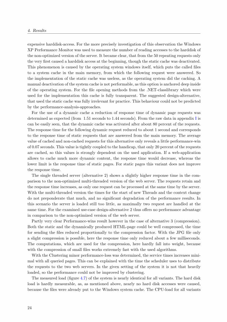
The measured load (figure 4.7) of the system is nearly identical for all variants. The hard diskload is hardly measurable, as, as mentioned above, nearly no hard disk accesses were caused,because the files were already put to the Windows system cache. The CPU-load for all variants
24
4.1. Validity of the prediction
7,36%7,86% 8,01%
7,07%
8,20%
6,27%
0,28% 0,25% 0,11%
0,84%
0,15%0,41%
0,00%
1,00%
2,00%
3,00%
4,00%
5,00%
6,00%
7,00%
8,00%
9,00%
10,00%
Alternative 0: keineOptimierung
Alternative 1a:Statischer Cache
Alternative 1b:Dynamischer Cache
Alternative 2: SingleThreaded
Alternative 3:Komprimierung
Alternative 4:Clustering
Aus
last
ung
in P
roze
nt
CPU Disk
Abbildung 4.7.: Load of the web server (measured); y-axis: load in percent; x-axis: alternative0 no optimization, alternative 1a static cache, alternative 1x dynamic cache,alternative 2 single threaded, alternative 3 compression, alternative 4 clustering;blue bar: CPU; red bar: disk
25
4. Results
is at the same level (within the measuring precision). For the single-threaded server the CPU-load is slightly less in comparison to the non-optimized variant. This could result from the factthat with this alternative in each case only one request is answered at the same time and theCPU is not used for the context change of threads, but the minor load of the CPU causes higherresponse-times. In the case of clustering the load is reduced as well. This can be explained by thedistribution of load to two servers. However the deviation of load is so little (about 1%) with both,the single threaded the server and the clustered server, that simple measurement inaccuraciescould be present, which can never be completely excluded with such an experimental setup.
4.1.5. Comparison of Predictions and Measurements
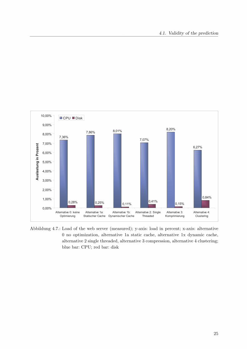
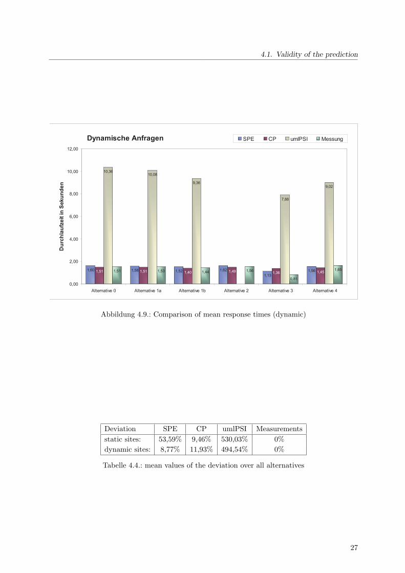
In figures 4.8 and 4.9 the predicted response times are displayed along with measurements ofthe implementation. The values for each individual prediction approach are the average valuesover the predictions of all participants, who predicted with this approach. With the SPE thereis only one value both for static and dynamic queries, this value appears in both diagrams.
Statische Anfragen
1,60 1,58 1,52 1,621,13
1,56
0,94 0,92 0,94 0,94 0,67 0,91
7,96
7,24 7,34
5,93
6,55
0,99 1,01 1,00 1,060,52
1,15
0,00
2,00
4,00
6,00
8,00
10,00
12,00
Alternative 0 Alternative 1a Alternative 1b Alternative 2 Alternative 3 Alternative 4
Dur
chla
ufze
it in
Sek
unde
n
SPE CP umlPSI Messung
Abbildung 4.8.: Comparison of mean response times (static)
With the SPE and the CP approaches the response times were predicted in each case witha user arrival rate by a user per second. With the umlPSI approach the user arrival rate hadto be individually tuned for each participant because of the problematic simulation. During themeasurements of the Web server the queries could not be generated by the test tool accurately inthe one-second pulse, however we tried to keep the deviation as small as possible. User requestswith higher arrival rates did not show large deviations in the results of measurement, so thatthe obtained results are sufficient for the comparison with the predictions. The high values forthe umlPSI stand out obviously in these diagrams. The proportional deviations of the responsetimes over all variants of the Web server can be seen in table ??.
26
4.1. Validity of the prediction
Dynamische Anfragen
1,60 1,58 1,52 1,621,13
1,561,51 1,51 1,40 1,49 1,36 1,45
10,3610,08
9,36
7,88
9,02
1,51 1,53 1,44 1,56
0,81
1,65
0,00
2,00
4,00
6,00
8,00
10,00
12,00
Alternative 0 Alternative 1a Alternative 1b Alternative 2 Alternative 3 Alternative 4
Dur
chla
ufze
it in
Sek
unde
n
SPE CP umlPSI Messung
Abbildung 4.9.: Comparison of mean response times (dynamic)
Deviation SPE CP umlPSI Measurementsstatic sites: 53,59% 9,46% 530,03% 0%dynamic sites: 8,77% 11,93% 494,54% 0%
Tabelle 4.4.: mean values of the deviation over all alternatives
27
4. Results
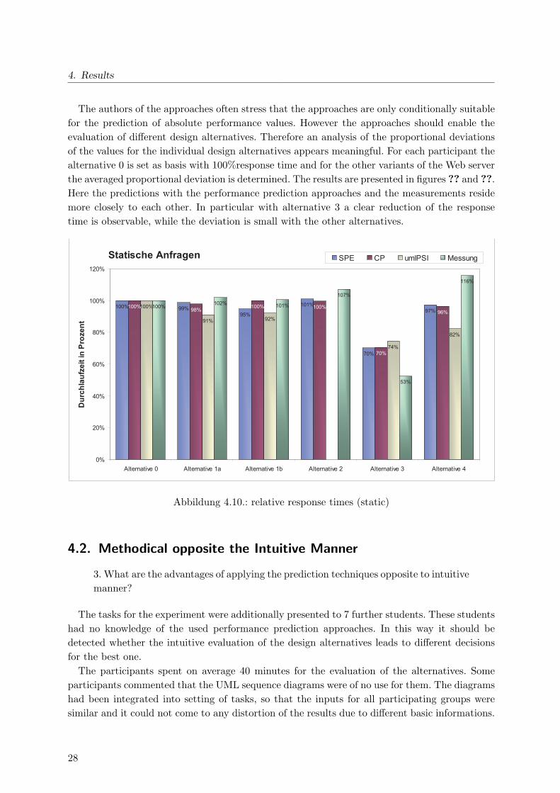
The authors of the approaches often stress that the approaches are only conditionally suitablefor the prediction of absolute performance values. However the approaches should enable theevaluation of different design alternatives. Therefore an analysis of the proportional deviationsof the values for the individual design alternatives appears meaningful. For each participant thealternative 0 is set as basis with 100%response time and for the other variants of the Web serverthe averaged proportional deviation is determined. The results are presented in figures ?? and ??.Here the predictions with the performance prediction approaches and the measurements residemore closely to each other. In particular with alternative 3 a clear reduction of the responsetime is observable, while the deviation is small with the other alternatives.
Statische Anfragen
100% 99%95%
101%
70%
97%100% 98% 100% 100%
70%
96%100%
91% 92%
74%
82%
100% 102% 101%
107%
53%
116%
0%
20%
40%
60%
80%
100%
120%
Alternative 0 Alternative 1a Alternative 1b Alternative 2 Alternative 3 Alternative 4
Dur
chla
ufze
it in
Pro
zent
SPE CP umlPSI Messung
Abbildung 4.10.: relative response times (static)
4.2. Methodical opposite the Intuitive Manner
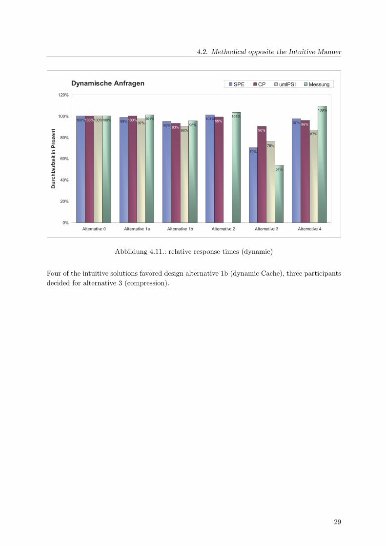
3. What are the advantages of applying the prediction techniques opposite to intuitivemanner?
The tasks for the experiment were additionally presented to 7 further students. These studentshad no knowledge of the used performance prediction approaches. In this way it should bedetected whether the intuitive evaluation of the design alternatives leads to different decisionsfor the best one.
The participants spent on average 40 minutes for the evaluation of the alternatives. Someparticipants commented that the UML sequence diagrams were of no use for them. The diagramshad been integrated into setting of tasks, so that the inputs for all participating groups weresimilar and it could not come to any distortion of the results due to different basic informations.
28
4.2. Methodical opposite the Intuitive Manner
Dynamische Anfragen
100% 99%95%
101%
70%
97%100% 100%
93%
99%
90%96%
100%97%
90%
76%
87%
100% 101%
95%
103%
54%
109%
0%
20%
40%
60%
80%
100%
120%
Alternative 0 Alternative 1a Alternative 1b Alternative 2 Alternative 3 Alternative 4
Dur
chla
ufze
it in
Pro
zent
SPE CP umlPSI Messung
Abbildung 4.11.: relative response times (dynamic)
Four of the intuitive solutions favored design alternative 1b (dynamic Cache), three participantsdecided for alternative 3 (compression).
29

30
5. Conclusions and Perspectives
The following chapter sums up this work and its results.
5.1. Summary
Each participant proposed one alternative out of the five given design-alternatives. The biggerpart (72%) favourised alternative 3, the compression of HTTP-requests. This design-alternativehad in fact (implementation) the slightest response-time of all alternatives.
The predicted absolute response-time gained by the approaches, particularly for some parti-cipants, differed several seconds from the measured data. The estimation of some performance-values of actions and resources was quite difficult for some participants. Anyway they couldevaluate the design-alternatives realistically by their relative differences. The predicted percen-tual performance-profit of the different design-alternatives could be determined with less than15% deviation to the measurements of the implementation.
The independent control-group of seven students, who didn’t know the performance-approachesfavourised a different design-alternative than the participants of the experiment. The majoritypreferred alternative 1b, which was the second fast alternative of the measured alternatives.This means that the tasks did not intuitively lead to alternative 3 from the 5 available design-alternatives.
A lot of properties of the approaches, like mightiness of the notation, the ergonomics ofthe tools or the evaluation-methods, have already been discussed. Most of the approaches areformally quite elaborated, but their practical usability and the availability of efficient tools isvery poor. The developers had to put a lot of manpower into the analyses to get realisticalresults and predictions. Especially the availability of UML and the UML performance-profilesis a starting-points that might let await a better integration of performance-analysis into theobject-oriented software-engineering.
The SPE-Approach of Smith and Williams is very usable for early performance-analysis ofsoftware-architectures. It is a approach which makes performance-predictions out of little input.The method is well evaluated after 20 years of research. The basical waiting-queue-model is wellencapsulated to reduce the complexity. At all this approach is easily usable for developers.
Anyway this approach reveals a break between software-modeling and performance-modeling.The used execution-graphs have to be created manually from the software-specification (e. g.UML), a automatic transformation is not offered by SPE-ED. As well a back-transformation ofthe performance-results to the software-specification is not intended. SPE-ED is not integratableinto other (CASE-) tools. Even there is no possibility to model the run-time-environment likein Java or to model the influence of application servers. The results of already measured andimplemented parts have be added manually to the performance-model. Not at least the GUIshould be improved.
31
5. Conclusions and Perspectives
The CP-approach is tightly coupled to the classical waiting-queue and is not useful for earlyperformance-prediction, but more for existing systems. After more than 30 years of research inwaiting-queues there exist a lot of algorithms and formulas to evaluate a big number of realcomputer systems. Often only approximated solutions can be created. For early performanceprediction it often is not worth creating complex models and employing with the mathematicalbackgrounds. The input parameters in the most cases are measured data and not estimations.The analysis mostly takes only the hardware-layer into account. A integration of software-modelsis not intended as well as coupling to software-tools.
umlPSI is a interesting approach. It uses UML diagrams out of which an automatically gene-rated simulation of performance-behaviour for a given architecture is done. Therefore the dia-gramms first have to be annotated with performance-data in the standardised UML PerformanceProfile. It is the first approach that uses this standard for simulations. After the simulation theresults can be transferred back to the diagrams. This approach is the only one which supportsa feedback-mechanism. It should not be underrated that the processing of raw data consumesa lot time. umlPSI is the approach out of the three which is the very most like ”real“ software-engineering. Developers might be convinced the easiest way of this performance-approach. Theyjust have to learn UML Performance Profile but no evaluation-methods.
Anyway umlPSI is just a prototype which does not work completely stable.Extensions for this tool might be a support for other types of UML-diagrams. The support
of further UML Profiles e. g. for reliability, safety and other Quality-of-Service-properties. Theprofiler allows to measure the run-time for readily implemented code-fragments. This way theestimation in the diagrams can be stated more precisely, the models can create improved overall-results.
32
Literaturverzeichnis
[BCR94] Victor R. Basili, Gianluigi Caldiera, and H. Dieter Rombach. The goal questionmetric approach. Encyclopedia of Software Engineering - 2 Volume Set, pages 528–532, 1994.
[GHJV95] E. Gamma, R. Helm, R. Johnson, and J. Vlissides. Design Patterns: Elements ofReusable Object-Oriented Systems. Addison-Wesley, 1995.
[Inc04] Web Performance Inc. Web performance trainer. http://www.webperformanceinc.com, 2004.
[Kil02] Patrick Killelea. Web Performance Tuning. O’Reilly, 2nd edition, 2002.
[Lib03] Jesse Liberty. Programming #. O’Reilly, 3rd edition, June 2003.
[MAD04] Daniel A. Menasce, Virgilio A.F. Almeida, and Lawrence W. Dowdy. Performanceby Design. Prentice Hall, 2004.
[Mar04] Moreno Marzolla. Simulation-Based Performance Modeling of UML Software Archi-tectures. PhD thesis, Universit‘a Ca Foscari di Venezia, 2004.
[Pre01] Lutz Prechelt. Kontrollierte Experimente in der Softwaretechnik. Springer Verlag,2001.
[Smi02] Connie U. Smith. Performance Solutions: A Practical Guide To Creating Responsive,Scalable Software. Addison-Wesley, 2002.
33

34
A. Vergleichstabelle
Performance-Analyseverfahren
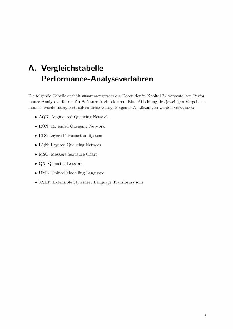
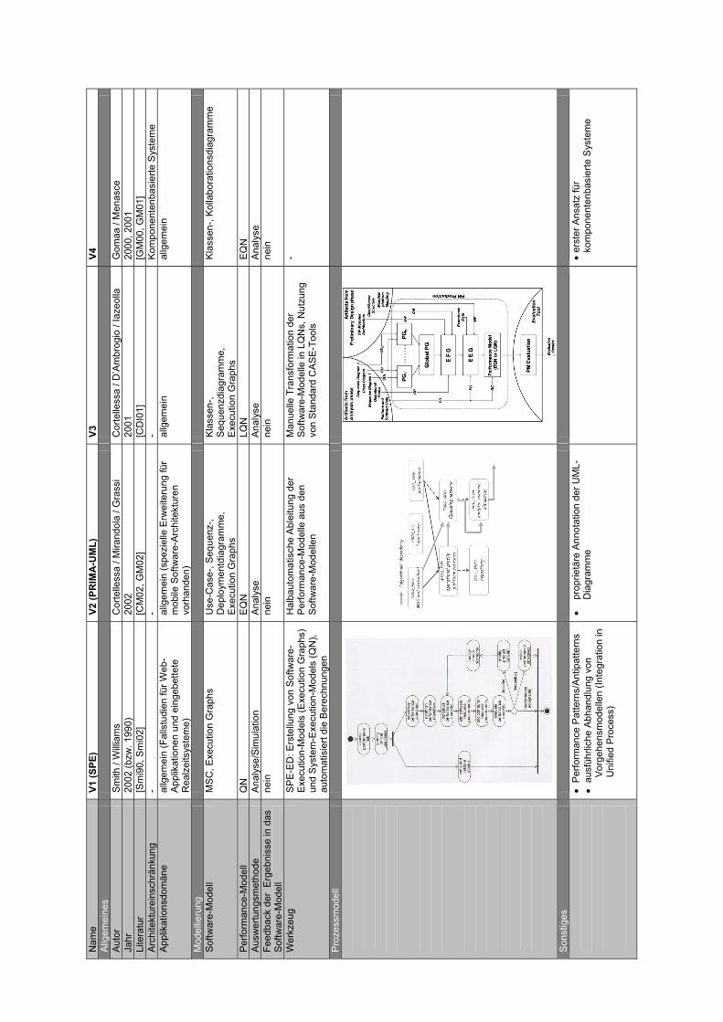
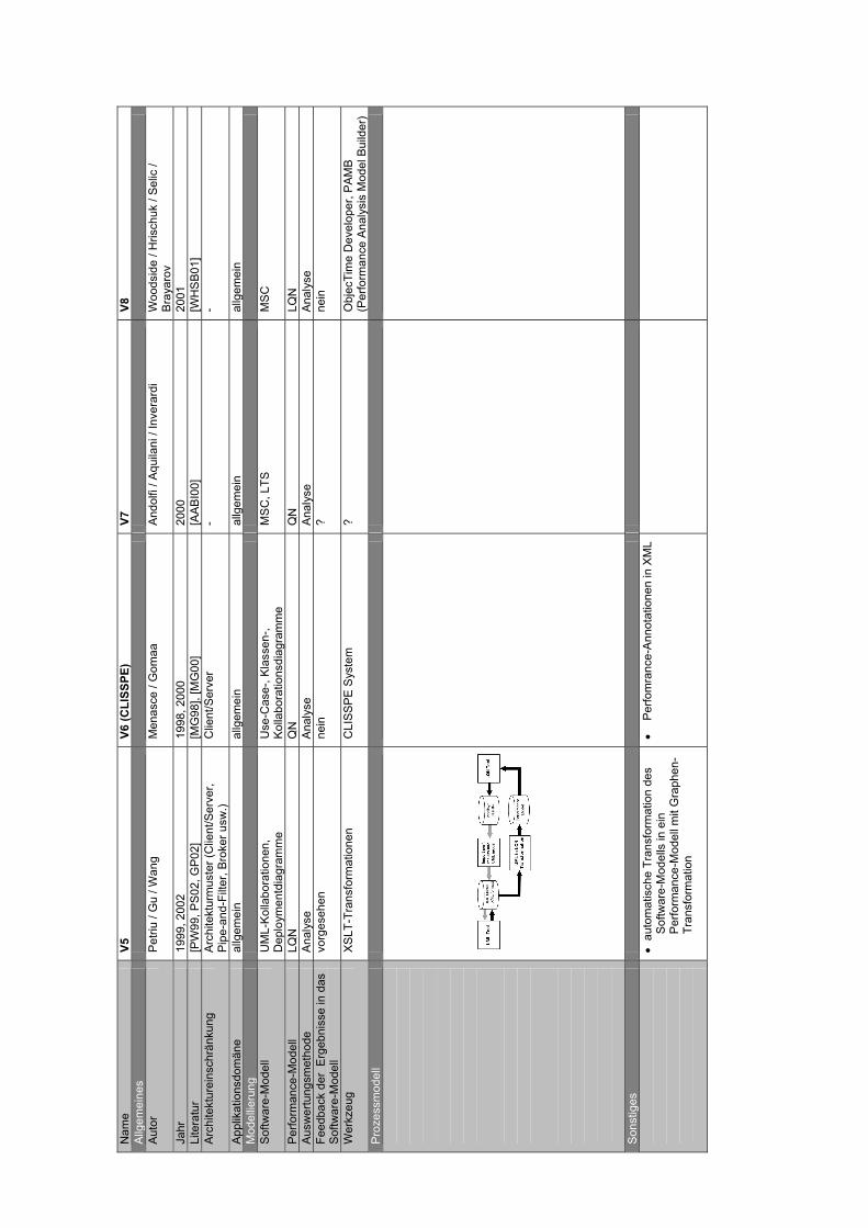
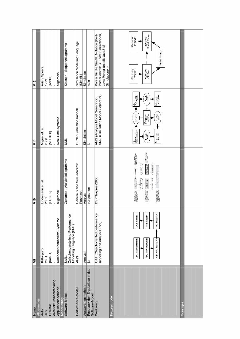
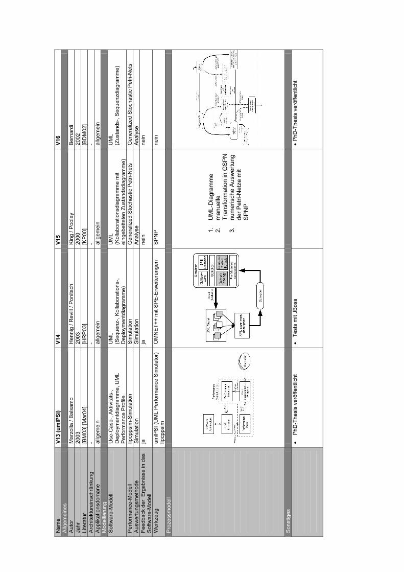
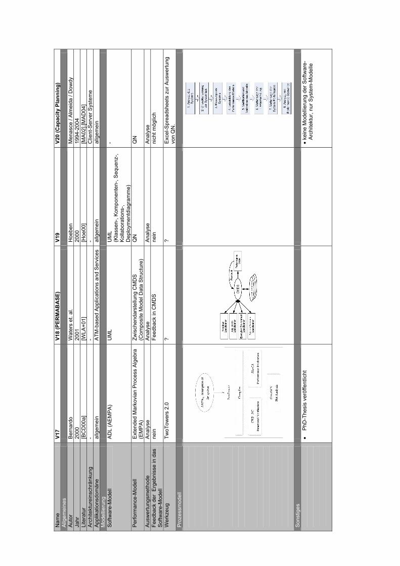
Die folgende Tabelle enthalt zusammengefasst die Daten der in Kapitel ?? vorgestellten Perfor-mance-Analyseverfahren fur Software-Architekturen. Eine Abbildung des jeweiligen Vorgehens-modells wurde intergriert, sofern diese vorlag. Folgende Abkurzungen werden verwendet:
• AQN: Augmented Queueing Network
• EQN: Extended Queueing Network
• LTS: Layered Transaction System
• LQN: Layered Queueing Network
• MSC: Message Sequence Chart
• QN: Queueing Network
• UML: Unified Modelling Language
• XSLT: Extensible Stylesheet Language Transformations
i
Nam
e V1
(SPE
) V2
(PR
IMA
-UM
L)
V3
V4
Allg
emei
nes
Aut
or
Sm
ith /
Will
iam
s C
orte
lless
a / M
irand
ola
/ Gra
ssi
Cor
telle
ssa
/ D’A
mbr
ogio
/ Ia
zeol
la
Gom
aa /
Men
asce
Ja
hr
2002
(bzw
. 199
0)
2002
20
01
2000
, 200
1 Li
tera
tur
[Sm
i90,
Sm
i02]
[C
M02
, GM
02]
[CD
I01]
[G
M00
, GM
01]
Arc
hite
ktur
eins
chrä
nkun
g -
- -
Kom
pone
nten
basi
erte
Sys
tem
e A
pplik
atio
nsdo
män
e al
lgem
ein
(Fal
lstu
dien
für W
eb-
App
likat
ione
n un
d ei
ngeb
ette
te
Rea
lzei
tsys
tem
e)
allg
emei
n (s
pezi
elle
Erw
eite
rung
für
mob
ile S
oftw
are-
Arc
hite
ktur
en
vorh
ande
n)
allg
emei
n al
lgem
ein
Mod
ellie
rung
S
oftw
are-
Mod
ell
MS
C, E
xecu
tion
Gra
phs
Use
-Cas
e-, S
eque
nz-,
Dep
loym
entd
iagr
amm
e,
Exe
cutio
n G
raph
s
Kla
ssen
-,
Seq
uenz
diag
ram
me,
E
xecu
tion
Gra
phs
Kla
ssen
-, K
olla
bora
tions
diag
ram
me
Per
form
ance
-Mod
ell
QN
E
QN
LQ
N
EQ
N
Aus
wer
tung
smet
hode
A
naly
se/S
imul
atio
n A
naly
se
Ana
lyse
A
naly
se
Feed
back
der
Erg
ebni
sse
in d
as
Sof
twar
e-M
odel
l ne
in
nein
ne
in
nein
Wer
kzeu
g S
PE
-ED
: Ers
tellu
ng v
on S
oftw
are-
Exe
cutio
n-M
odel
s (E
xecu
tion
Gra
phs)
un
d S
yste
m-E
xecu
tion-
Mod
els
(QN
), au
tom
atis
iert
die
Ber
echn
unge
n
Hal
baut
omat
isch
e A
blei
tung
der
P
erfo
rman
ce-M
odel
le a
us d
en
Sof
twar
e-M
odel
len
Man
uelle
Tra
nsfo
rmat
ion
der
Sof
twar
e-M
odel
le in
LQ
Ns,
Nut
zung
vo
n S
tand
ard
CA
SE
-Too
ls
-
Pro
zess
mod
ell
Son
stig
es
• P
erfo
rman
ce P
atte
rns/
Ant
ipat
tern
s •
ausf
ührli
che
Abh
andl
ung
von
Vor
gehe
nsm
odel
len
(Inte
grat
ion
in
Uni
fied
Pro
cess
)
• pr
oprie
täre
Ann
otat
ion
der U
ML-
Dia
gram
me
•
erst
er A
nsat
z fü
r ko
mpo
nent
enba
sier
te S
yste
me
Nam
e V5
V6
(CLI
SSPE
) V7
V8
A
llgem
eine
s
A
utor
P
etriu
/ G
u / W
ang
Men
asce
/ G
omaa
A
ndol
fi / A
quila
ni /
Inve
rard
i W
oods
ide
/ Hris
chuk
/ S
elic
/ B
raya
rov
Jahr
19
99, 2
002
1998
, 200
0 20
00
2001
Li
tera
tur
[PW
99, P
S02
, GP
02]
[MG
98],
[MG
00]
[AA
BI0
0]
[WH
SB
01]
Arc
hite
ktur
eins
chrä
nkun
g A
rchi
tekt
urm
uste
r (C
lient
/Ser
ver,
Pip
e-an
d-Fi
lter,
Bro
ker u
sw.)
Clie
nt/S
erve
r -
-
App
likat
ions
dom
äne
allg
emei
n al
lgem
ein
allg
emei
n al
lgem
ein
Mod
ellie
rung
S
oftw
are-
Mod
ell
UM
L-K
olla
bora
tione
n,
Dep
loym
entd
iagr
amm
e U
se-C
ase-
, Kla
ssen
-, K
olla
bora
tions
diag
ram
me
MS
C, L
TS
MS
C
Per
form
ance
-Mod
ell
LQN
Q
N
QN
LQ
N
Aus
wer
tung
smet
hode
A
naly
se
Ana
lyse
A
naly
se
Ana
lyse
Fe
edba
ck d
er E
rgeb
niss
e in
das
S
oftw
are-
Mod
ell
vorg
eseh
en
nein
?
nein
Wer
kzeu
g X
SLT
-Tra
nsfo
rmat
ione
n C
LIS
SP
E S
yste
m
? O
bjec
Tim
e D
evel
oper
, PA
MB
(P
erfo
rman
ce A
naly
sis
Mod
el B
uild
er)
Pro
zess
mod
ell
Son
stig
es
• au
tom
atis
che
Tran
sfor
mat
ion
des
Sof
twar
e-M
odel
ls in
ein
P
erfo
rman
ce-M
odel
l mit
Gra
phen
-Tr
ansf
orm
atio
n
• P
erfo
mra
nce-
Ann
otat
ione
n in
XM
L
Nam
e V9
V1
0 V1
1 V1
2 A
llgem
eine
s
A
utor
K
ähki
puro
Li
ndem
ann
et. a
l. M
igue
l et.
al.
Arie
f / S
pear
s Ja
hr
2001
20
02
2000
19
99
Lite
ratu
r [K
äh01
] [L
TK+0
2]
[MLH
+00]
[A
S99
] A
rchi
tekt
urei
nsch
ränk
ung
- -
- -
App
likat
ions
dom
äne
Kom
pone
nten
basi
erte
Sys
tem
e al
lgem
ein
Rea
l-Tim
e-S
yste
ms
allg
emei
n M
odel
lieru
ng
Sof
twar
e-M
odel
l U
ML,
Zw
isch
enda
rste
llung
Per
form
ance
M
odel
ling
Lang
uage
(PM
L)
Zust
ands
-, A
ktiv
itäts
diag
ram
me
UM
L K
lass
en-,
Seq
uenz
diag
ram
me
Per
form
ance
-Mod
ell
AQ
N
Gen
eral
isie
rte S
emi-M
arko
w
Pro
zess
e O
PN
et S
imul
atio
nsm
odel
l S
imul
atio
n M
odel
ling
Lang
uage
(S
imM
L)
Aus
wer
tung
smet
hode
A
naly
se
Ana
lyse
S
imul
atio
n S
imul
atio
n Fe
edba
ck d
er E
rgeb
niss
e in
das
S
oftw
are-
Mod
ell
ja
vorg
eseh
en
ja
nein
Wer
kzeu
g O
AT
(Obj
ect-o
rient
ed p
erfo
rman
ce
mod
ellin
g an
d A
naly
sis
Tool
) D
SP
Nex
pres
s200
0 A
MG
(Ana
lysi
s M
odel
Gen
erat
or)
SM
G (S
imul
atio
n M
odel
Gen
erat
or)
Par
ser f
ür d
ie S
imM
L N
otat
ion
(Per
l-P
arse
r ers
tellt
C++
SIM
Sim
ulat
ione
n,
Java
-Par
ser e
rste
llt J
avaS
IM
Sim
ulat
ione
n)
Pro
zess
mod
ell
Son
stig
es
Nam
e V1
3 (u
mlP
SI)
V14
V15
V16
Allg
emei
nes
Aut
or
Mar
zolla
/ B
alsa
mo
Hen
nig
/ Rev
ill /
Pon
itsch
K
ing
/ Poo
ley
B
erna
rdi
Jahr
20
03
2003
20
00
2002
Li
tera
tur
[BM
03] [
Mar
04]
[HR
P03
] [K
P00
] [B
DM
02]
Arc
hite
ktur
eins
chrä
nkun
g -
- -
- A
pplik
atio
nsdo
män
e al
lgem
ein
allg
emei
n al
lgem
ein
allg
emei
n M
odel
lieru
ng
Sof
twar
e-M
odel
l U
se-C
ase-
, Akt
ivitä
ts-,
Dep
loym
entd
iagr
amm
e, U
ML
Per
form
ance
Pro
file
UM
L (S
eque
nz-,
Kol
labo
ratio
ns-,
Dep
loym
entd
iagr
amm
e)
UM
L (K
olla
bora
tions
diag
ram
me
mit
eing
ebet
tete
n Zu
stan
dsdi
agra
mm
e)
UM
L (Z
usta
nds-
, Seq
uenz
diag
ram
me)
Per
form
ance
-Mod
ell
lipcp
psim
-Sim
ulat
ion
Sim
ulat
ion
Gen
eral
ized
Sto
chas
tic P
etri-
Net
s G
ener
aliz
ed S
toch
astic
Pet
ri-N
ets
Aus
wer
tung
smet
hode
S
imul
atio
n S
imul
atio
n A
naly
se
Ana
lyse
Fe
edba
ck d
er E
rgeb
niss
e in
das
S
oftw
are-
Mod
ell
ja
ja
nein
ne
in
Wer
kzeu
g um
lPS
I (U
ML
Per
form
ance
Sim
ulat
or)
lipcp
psim
O
MN
ET+
+ m
it S
PE
-Erw
eite
rung
en
SP
NP
ne
in
Pro
zess
mod
ell
1.
UM
L-D
iagr
amm
e 2.
m
anue
lle
Tran
sfor
mat
ion
in G
SP
N
3.
num
eris
che
Aus
wer
tung
de
r Pet
ri-N
etze
mit
SP
NP
Son
stig
es
• P
hD-T
hesi
s ve
röffe
ntlic
ht
• Te
sts
mit
JBos
s
• P
hD-T
hesi
s ve
röffe
ntlic
ht
Nam
e V1
7 V1
8 (P
ERM
AB
ASE
) V1
9 V2
0 (C
apac
ity P
lann
ing)
A
llgem
eine
s
A
utor
B
erna
rdo
Wat
ers
et. a
l. H
oebe
n M
enas
ce /
Alm
eida
/ D
owdy
Ja
hr
2000
20
01
2000
19
94-2
004
Lite
ratu
r [B
CD
00a]
[W
LA+0
1]
[Hoe
00]
[MA
02],[
MA
D04
] A
rchi
tekt
urei
nsch
ränk
ung
- -
- C
lient
-Ser
ver S
yste
me
App
likat
ions
dom
äne
allg
emei
n A
TM-b
ased
App
licat
ions
and
Ser
vice
s al
lgem
ein
allg
emei
n M
odel
lieru
ng
Sof
twar
e-M
odel
l A
DL
(AE
MP
A)
UM
L U
ML
(Kla
ssen
-, K
ompo
nent
en-,
Seq
uenz
-, K
olla
bora
tions
-, D
eplo
ymen
tdia
gram
me)
-
Per
form
ance
-Mod
ell
Ext
ende
d M
arko
vian
Pro
cess
Alg
ebra
(E
MP
A)
Zwis
chen
dars
tellu
ng C
MD
S
(Com
posi
te M
odel
Dat
a S
truct
ure)
Q
N
QN
Aus
wer
tung
smet
hode
A
naly
se
Ana
lyse
A
naly
se
Ana
lyse
Fe
edba
ck d
er E
rgeb
niss
e in
das
S
oftw
are-
Mod
ell
nein
Fe
edba
ck in
CM
DS
ne
in
nich
t mög
lich
Wer
kzeu
g Tw
oTow
ers
2.0
? ?
Exc
el-S
prea
dshe
ets
zur A
usw
ertu
ng
von
QN
. P
roze
ssm
odel
l
S
onst
iges
• P
hD-T
hesi
s ve
röffe
ntlic
ht
• ke
ine
Mod
ellie
rung
der
Sof
twar
e-A
rchi
tekt
ur, n
ur S
yste
m-M
odel
le
B. Folien der Ubungen
Zum Training der Versuchsteilnehmer wurde fur jedes untersuchte Verfahren ein Foliensatz zu-sammengestellt. Die enthaltenen Abbildungen und Beispiele entstammen jeweils aus der zu-gehorigen Literatur [Smi02], [MAD04], [Mar04]. Mit den Folien kann nachvollzogen werden, aufwelcher Wissenbasis die Versuchsteilnehmer ihre Performance-Analysen durchfuhrten.
vii
1
Software Performance Engineering (SPE)
Smith/Williams
31.08.2004 Software Performance Engineering 2
Inhalt• Allgemeines• Vorgehensmodell• SPE und UML
– erweiterte Sequenzdiagramme• Software Execution Models
– Execution Graphs• System Execution Models
– Queueing Network• Performance-orientiertes Design• Beispiel
31.08.2004 Software Performance Engineering 3
Allgemeines
• 1981: Prägung des Begriffs „Software Performance Engineering“ durch Connie U. Smith
• 1990: Buch „Performance Engineering of Software Systems“– erste vollständige Methode zur Performance-
Analyse von Software-Systemen während des Entwurfs
• 2002: Buch „Performance Solutions“– Integration der UML– Anpassungen für verteilte bzw. eingebettete
Systeme– Tool SPE-ED– Performance-Patterns/Antipatterns
31.08.2004 Software Performance Engineering 4
SPE-Vorgehensmodell
31.08.2004 Software Performance Engineering 5
Vorgehensmodell• Beispiel: Entwurf eines
Geldautomaten
31.08.2004 Software Performance Engineering 6
Vorgehensmodell• Festlegung des Umfangs des SPE-
Projekts je nach Signifikanz der Performance
• Erstellung eines detaillierterenModells bei Performance-kritischeren Anwendungen
• Beispiel Geldautomat: geringes Performance-Risiko, einfaches Modell ausreichend
2
31.08.2004 Software Performance Engineering 7
Vorgehensmodell
31.08.2004 Software Performance Engineering 8
Vorgehensmodell
31.08.2004 Software Performance Engineering 9
Vorgehensmodell• Konkrete Vorgaben für z.B.
Antwortszeiten, Durchsatz, Ressourcennutzung usw.
• Beispiel Geldautomat: „Die Bedienung darf nicht länger als 30 Sekunden dauern.“
31.08.2004 Software Performance Engineering 10
Vorgehensmodell• Transformation der Sequenzdiagramme in
Ausführungsgraphen
31.08.2004 Software Performance Engineering 11
Vorgehensmodell• Transformation der Sequenzdiagramme in
Ausführungsgraphen
31.08.2004 Software Performance Engineering 12
Vorgehensmodell• Bestimmung der Anforderungen von
Software-Elementen
3
31.08.2004 Software Performance Engineering 13
Vorgehensmodell• Bestimmung der Anforderungen von
Hardware-Elementen
31.08.2004 Software Performance Engineering 14
Vorgehensmodell• Berechnung der Performance-Werte• Beispiel Geldautomat: „Die
Bedienung dauert 29 Sekunden und ist somit knapp innerhalb der Vorgaben“
• bei Nichteinhaltung der Vorgaben:– Modifikation der Software– Modifikation der Szenarien– Überarbeitung der Performance-Ziele
31.08.2004 Software Performance Engineering 15
SPE und UML
31.08.2004 Software Performance Engineering 16
SPE und UML• UML: Standard-Notation für die Modellierung
objektorientierter Systeme• Basis für die Erstellung des Performance-
Modells • Erweiterungen der UML für Performance-
spezifische Informationen (angelehnt an Message Sequence Charts)– hierarchische Strukturierung von
Sequenzdiagrammen– graphische Repräsentation von Schleifen und
Auswahlknoten in Sequenzdiagrammen– Nebenläufigkeit in Sequenzdiagrammen
31.08.2004 Software Performance Engineering 17
Beispiel: Erweiterte Sequenzdiagramme
Schleife: gebunden an Schleifenklausel
Auswahl: gebunden an Bedingungsklausel
Referenz:verzweigt in ein weiteres Sequenzdiagramm
31.08.2004 Software Performance Engineering 18
Sequenzdiagramme: Kontrollfluss
• Prozeduraufrufe: Fortsetzung der Ausführung erst nach Beendigung aller verschachtelten Aufrufe
• Nichtprozeduraler Aufruf: nächster Schritt in der Sequenz
• Asynchrone Kommunikationen zwischen zwei Objekten
• return-Anweisung eines Prozeduraufrufs

4
31.08.2004 Software Performance Engineering 19
Erweiterte Features für Sequenzdiagramme:
• Referenz– Details in einem weiteren Sequenzdiagramm
• Iteration– n-malige Wiederholung des eingeschlossenen
Abschnitts• Alternative
– Ausführung genau eines Abschnittes gemäßder Bedingungsklausel
• Optionale Abschnitte– Ausführung des eingeschlossenen Abschnitts
optional gemäß der Bedingungsklausel• Parallele Abschnitte
– gleichzeitige Ausführung der eingeschlossenen Abschnitte
loop
alt
opt
par
31.08.2004 Software Performance Engineering 20
Software Execution Models
31.08.2004 Software Performance Engineering 21
Vom Sequenzdiagramm zum Ausführungsgraph
• Execution Graph– Modell zur vereinfachten Aufnahme von
Performance-Informationen– Ähnlichkeit mit UML-Aktivitätsdiagrammen
• Umwandlung jedes Aufrufes im Sequenzdiagramm in einen Knoten
• Zusammenfassung verwandter bzw. Performance-unkritischer Aufrufe in einen einzigen Knoten
• Ergänzung von Ausführungshäufigkeiten / -wahrscheinlichkeiten
31.08.2004 Software Performance Engineering 22
Beispiel: Sequenzdiagramm -> Ausführungsgraph
31.08.2004 Software Performance Engineering 23
Beispiel: Sequenzdiagramm -> Ausführungsgraph
31.08.2004 Software Performance Engineering 24
Ausführungsgraphen• Basisknoten
– Funktionale Komponente• Erweiterter Knoten
– Verfeinerte Funktion in einem Subgraphen• Wiederholungsknoten
– Schleife: n-malige Wiederholung einer Reihe von Knoten• Entscheidungsknoten
– Ausführung geknüpft an Bedingung– versehen mit Wahrscheinlichkeit
• Parallelknoten– parallele Ausführung von Knoten– Fortsetzung des Kontrollflusses erst nach Berechnung aller
Knoten• Spaltungsknoten
– parallele Ausführung von Knoten– Fortsetzung des Kontrollflusses auch wenn nicht alle Knoten
berechnet wurden
n
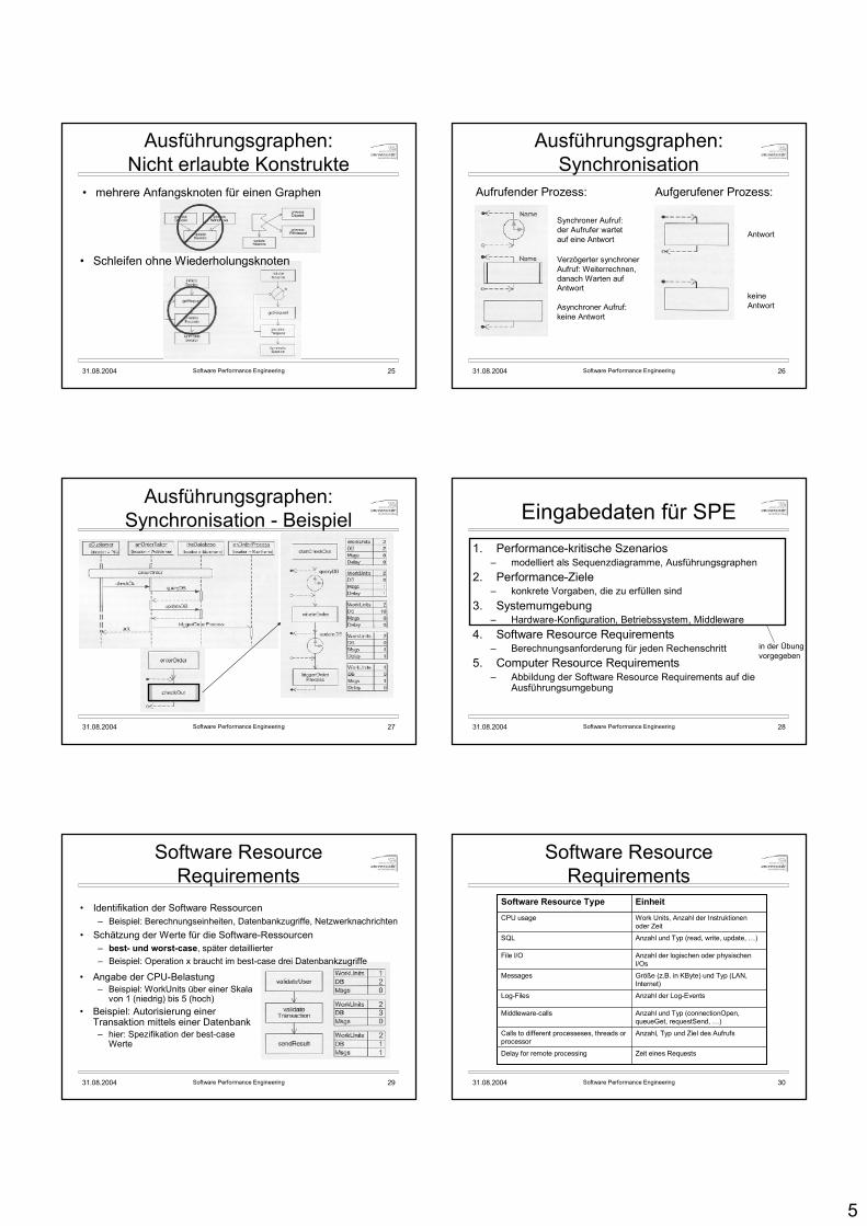
5
31.08.2004 Software Performance Engineering 25
Ausführungsgraphen:Nicht erlaubte Konstrukte
• mehrere Anfangsknoten für einen Graphen
• Schleifen ohne Wiederholungsknoten
31.08.2004 Software Performance Engineering 26
Ausführungsgraphen: Synchronisation
Aufrufender Prozess:
Synchroner Aufruf: der Aufrufer wartet auf eine Antwort
Verzögerter synchroner Aufruf: Weiterrechnen, danach Warten auf Antwort
Asynchroner Aufruf: keine Antwort
Aufgerufener Prozess:
Antwort
keine Antwort
31.08.2004 Software Performance Engineering 27
Ausführungsgraphen: Synchronisation - Beispiel
31.08.2004 Software Performance Engineering 28
Eingabedaten für SPE1. Performance-kritische Szenarios
– modelliert als Sequenzdiagramme, Ausführungsgraphen2. Performance-Ziele
– konkrete Vorgaben, die zu erfüllen sind3. Systemumgebung
– Hardware-Konfiguration, Betriebssystem, Middleware4. Software Resource Requirements
– Berechnungsanforderung für jeden Rechenschritt5. Computer Resource Requirements
– Abbildung der Software Resource Requirements auf die Ausführungsumgebung
in der Übungvorgegeben
31.08.2004 Software Performance Engineering 29
Software ResourceRequirements
• Angabe der CPU-Belastung – Beispiel: WorkUnits über einer Skala
von 1 (niedrig) bis 5 (hoch)• Beispiel: Autorisierung einer
Transaktion mittels einer Datenbank– hier: Spezifikation der best-case
Werte
• Identifikation der Software Ressourcen – Beispiel: Berechnungseinheiten, Datenbankzugriffe, Netzwerknachrichten
• Schätzung der Werte für die Software-Ressourcen – best- und worst-case, später detaillierter– Beispiel: Operation x braucht im best-case drei Datenbankzugriffe
31.08.2004 Software Performance Engineering 30
Software ResourceRequirements
Zeit eines RequestsDelay for remote processing
Anzahl, Typ und Ziel des AufrufsCalls to different processeses, threads orprocessor
Anzahl und Typ (connectionOpen, queueGet, requestSend, …)
Middleware-calls
Anzahl der Log-EventsLog-Files
Größe (z.B. in KByte) und Typ (LAN, Internet)
Messages
Anzahl der logischen oder physischen I/Os
File I/O
Anzahl und Typ (read, write, update, …)SQL
Work Units, Anzahl der Instruktionen oder Zeit
CPU usage
EinheitSoftware Resource Type
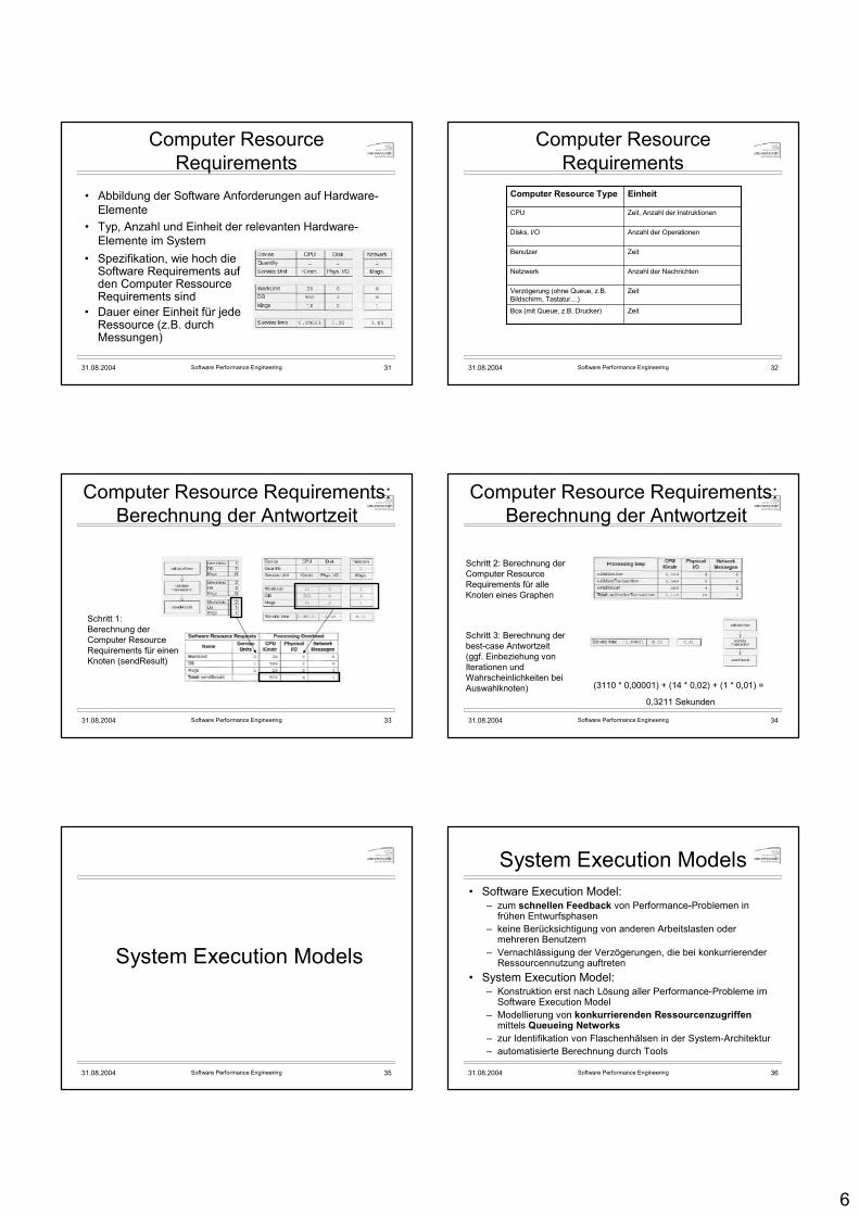
6
31.08.2004 Software Performance Engineering 31
Computer ResourceRequirements
• Abbildung der Software Anforderungen auf Hardware-Elemente
• Typ, Anzahl und Einheit der relevanten Hardware-Elemente im System
• Spezifikation, wie hoch die Software Requirements auf den Computer Ressource Requirements sind
• Dauer einer Einheit für jede Ressource (z.B. durch Messungen)
31.08.2004 Software Performance Engineering 32
Computer ResourceRequirements
ZeitBox (mit Queue, z.B. Drucker)
ZeitVerzögerung (ohne Queue, z.B. Bildschirm, Tastatur…)
Anzahl der NachrichtenNetzwerk
ZeitBenutzer
Anzahl der OperationenDisks, I/O
Zeit, Anzahl der InstruktionenCPU
EinheitComputer Resource Type
31.08.2004 Software Performance Engineering 33
Computer Resource Requirements: Berechnung der Antwortzeit
Schritt 1:Berechnung der Computer ResourceRequirements für einen Knoten (sendResult)
31.08.2004 Software Performance Engineering 34
Computer Resource Requirements:Berechnung der Antwortzeit
Schritt 2: Berechnung der Computer ResourceRequirements für alle Knoten eines Graphen
Schritt 3: Berechnung der best-case Antwortzeit (ggf. Einbeziehung von Iterationen und Wahrscheinlichkeiten bei Auswahlknoten) (3110 * 0,00001) + (14 * 0,02) + (1 * 0,01) =
0,3211 Sekunden
31.08.2004 Software Performance Engineering 35
System Execution Models
31.08.2004 Software Performance Engineering 36
System Execution Models• Software Execution Model:
– zum schnellen Feedback von Performance-Problemen in frühen Entwurfsphasen
– keine Berücksichtigung von anderen Arbeitslasten oder mehreren Benutzern
– Vernachlässigung der Verzögerungen, die bei konkurrierender Ressourcennutzung auftreten
• System Execution Model:– Konstruktion erst nach Lösung aller Performance-Probleme im
Software Execution Model– Modellierung von konkurrierenden Ressourcenzugriffen
mittels Queueing Networks– zur Identifikation von Flaschenhälsen in der System-Architektur– automatisierte Berechnung durch Tools
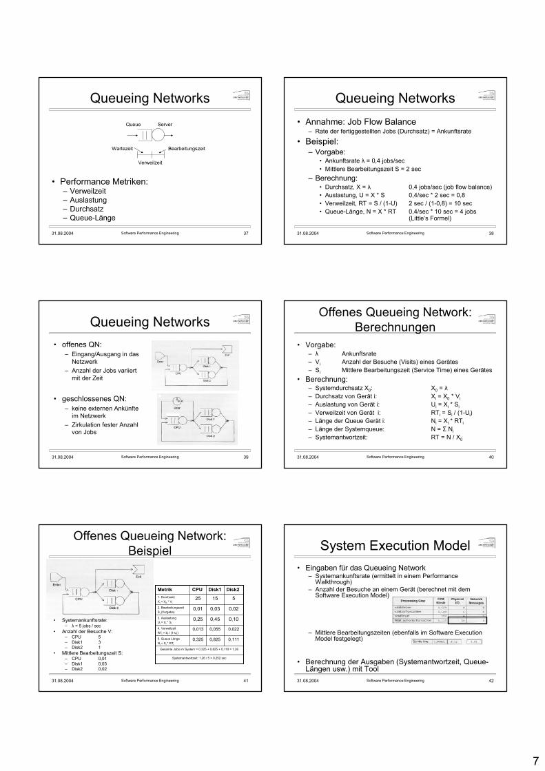
7
31.08.2004 Software Performance Engineering 37
Queueing Networks
• Performance Metriken:– Verweilzeit– Auslastung– Durchsatz– Queue-Länge
Queue Server
Wartezeit Bearbeitungszeit
Verweilzeit
31.08.2004 Software Performance Engineering 38
Queueing Networks• Annahme: Job Flow Balance
– Rate der fertiggestellten Jobs (Durchsatz) = Ankunftsrate
• Beispiel:– Vorgabe:
• Ankunftsrate λ = 0,4 jobs/sec• Mittlere Bearbeitungszeit S = 2 sec
– Berechnung:• Durchsatz, X = λ 0,4 jobs/sec (job flow balance)• Auslastung, U = X * S 0,4/sec * 2 sec = 0,8• Verweilzeit, RT = S / (1-U) 2 sec / (1-0,8) = 10 sec• Queue-Länge, N = X * RT 0,4/sec * 10 sec = 4 jobs
(Little‘s Formel)
31.08.2004 Software Performance Engineering 39
Queueing Networks• offenes QN:
– Eingang/Ausgang in das Netzwerk
– Anzahl der Jobs variiert mit der Zeit
• geschlossenes QN:– keine externen Ankünfte
im Netzwerk– Zirkulation fester Anzahl
von Jobs
31.08.2004 Software Performance Engineering 40
Offenes Queueing Network: Berechnungen
• Vorgabe:– λ Ankunftsrate– Vi Anzahl der Besuche (Visits) eines Gerätes– Si Mittlere Bearbeitungszeit (Service Time) eines Gerätes
• Berechnung:– Systemdurchsatz X0: X0 = λ– Durchsatz von Gerät i: Xi = X0 * Vi– Auslastung von Gerät i: Ui = Xi * Si– Verweilzeit von Gerät i: RTi = Si / (1-Ui)– Länge der Queue Gerät i: Ni = Xi * RTi– Länge der Systemqueue: N = Σ Ni– Systemantwortzeit: RT = N / X0
31.08.2004 Software Performance Engineering 41
Offenes Queueing Network: Beispiel
• Systemankunftsrate: – λ = 5 jobs / sec
• Anzahl der Besuche V:– CPU 5– Disk1 3– Disk2 1
• Mittlere Bearbeitungszeit S:– CPU 0,01– Disk1 0,03– Disk2 0,02
Systemantwortzeit: 1,26 / 5 = 0,252 sec
Gesamte Jobs im System = 0,325 + 0,825 + 0,110 = 1,26
0,1110,8250,3255. Queue LängeNi = Xi * RTi
0,0220,0550,0134. VerweilzeitRTi = Si / (1-Ui)
0,100,450,253. AuslastungUi = Xi * Si
0,020,030,012. BearbeitungszeitSi (Vorgabe)
515251. Durchsatz Xi = X0 * Vi
Disk2Disk1CPUMetrik
31.08.2004 Software Performance Engineering 42
System Execution Model• Eingaben für das Queueing Network
– Systemankunftsrate (ermittelt in einem Performance Walkthrough)
– Anzahl der Besuche an einem Gerät (berechnet mit dem Software Execution Model)
– Mittlere Bearbeitungszeiten (ebenfalls im Software ExecutionModel festgelegt)
• Berechnung der Ausgaben (Systemantwortzeit, Queue-Längen usw.) mit Tool
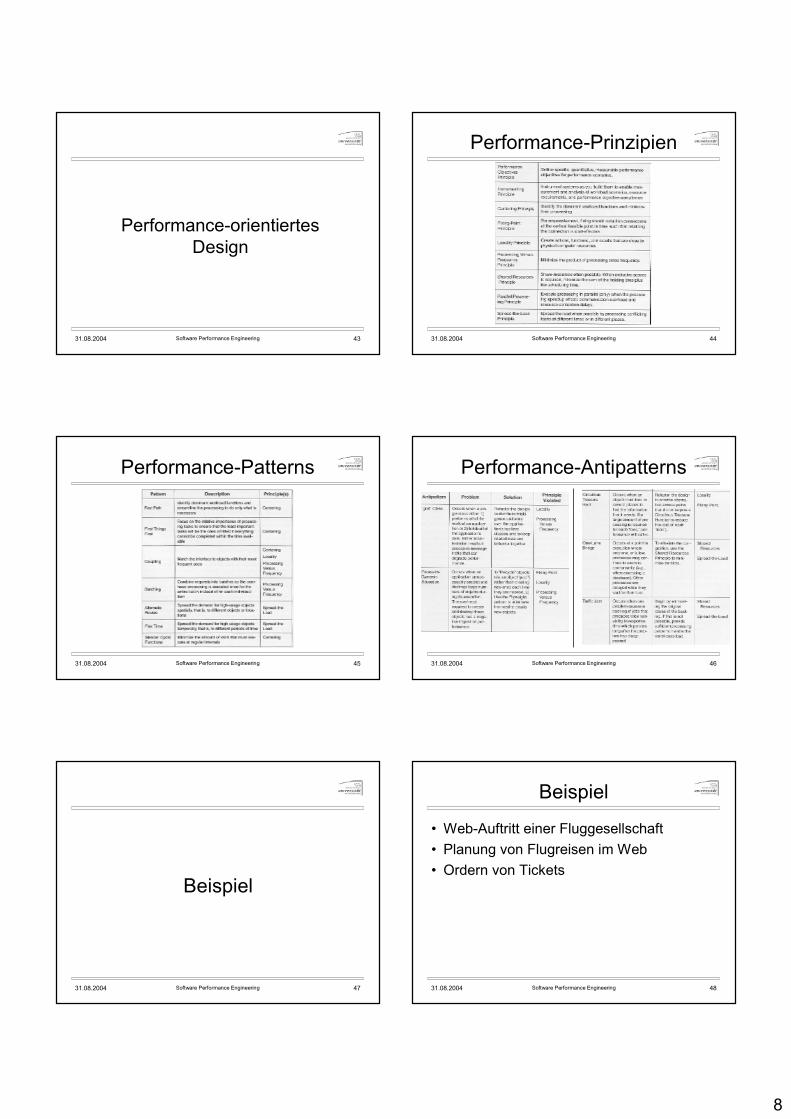
8
31.08.2004 Software Performance Engineering 43
Performance-orientiertes Design
31.08.2004 Software Performance Engineering 44
Performance-Prinzipien
31.08.2004 Software Performance Engineering 45
Performance-Patterns
31.08.2004 Software Performance Engineering 46
Performance-Antipatterns
31.08.2004 Software Performance Engineering 47
Beispiel
31.08.2004 Software Performance Engineering 48
Beispiel
• Web-Auftritt einer Fluggesellschaft• Planung von Flugreisen im Web• Ordern von Tickets

9
31.08.2004 Software Performance Engineering 49
1. Eingrenzen des Performance-Risikos
• mittleres Performance-Risiko• bei schlechter Performance: keine
Benutzung der Website -> Umsatzeinbußen
31.08.2004 Software Performance Engineering 50
2. Performance-kritische Use-Cases
31.08.2004 Software Performance Engineering 51
3. Modellierung von SzenarienplanItinerary
31.08.2004 Software Performance Engineering 52
3. Modellierung von Szenarien
login
31.08.2004 Software Performance Engineering 53
3. Modellierung von Szenarien
getFlightPlanningPage
31.08.2004 Software Performance Engineering 54
4. Festlegung von Performance-Zielen
• maximale Login-Zeit: 8 Sekunden• ansonsten zunächst keine Vorgaben
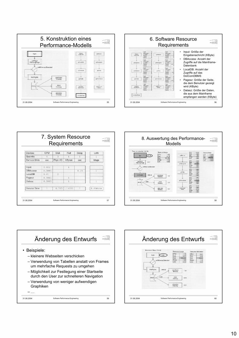
10
31.08.2004 Software Performance Engineering 55
5. Konstruktion eines Performance-Modells
31.08.2004 Software Performance Engineering 56
6. Software ResourceRequirements
• Input: Größe der Eingabenachricht (KByte)
• DBAccess: Anzahl der Zugriffe auf die Mainframe-Datenbank
• LocalDB: Anzahl der Zugriffe auf das DotComDBMS
• Pagesz: Größe der Seite, die dem Benutzer gezeigt wird (KByte)
• Datasz: Größe der Daten, die aus dem Mainframe empfangen werden (KByte)
31.08.2004 Software Performance Engineering 57
7. System ResourceRequirements
31.08.2004 Software Performance Engineering 58
8. Auswertung des Performance-Modells
31.08.2004 Software Performance Engineering 59
Änderung des Entwurfs
• Beispiele:– kleinere Webseiten verschicken– Verwendung von Tabellen anstatt von Frames
um mehrfache Requests zu umgehen– Möglichkeit zur Festlegung einer Startseite
durch den User zur schnelleren Navigation– Verwendung von weniger aufwendigen
Graphiken– …
31.08.2004 Software Performance Engineering 60
Änderung des Entwurfs

11
31.08.2004 Software Performance Engineering 61
Fazit: Lernziele der Übung
• Verstehen des SPE-Prozesses• Wissen, wie ein Sequenzdiagramm in einen
Ausführungsgraphen transformiert wird• Wissen, wie Software Resource Requirements
festgelegt werden• Wissen, wie Computer Resource Requirements
festgelegt werden, und wie damit Performance-Werte berechnet werden können
1
Capacity Planning
Menasce / Almeida
31.08.2004 Performance by Design 2
Inhalt
• Allgemeines• Vorgehensmodell• Workload-Modellierung• Queueing Networks
– qualitative Aspekte– quantitative Aspekte
• Beispiel
31.08.2004 Performance by Design 3
Allgemeines• seit Anfang der 70er: Einsatz von Queueing
Networks in der Performance-Analyse• 1994: „Capacity Planning and Performance
Modeling: from mainframes to client-serversystems“
• 1998: „Capacity Planning for Web Performance: metrics, models, and methods“
• 2000: „Scaling for E-Business: technologies, models, performance, and capacity planning“
• 2002: „Capacity Planning for Web Services“• 2004: „Performance by Design“
31.08.2004 Performance by Design 4
Vorgehensmodell
31.08.2004 Performance by Design 5
Vorgehensmodell
• Beispiel: Performance-Modellierung eines einfachen Web-Servers
31.08.2004 Performance by Design 6
Vorgehensmodell• Verstehen der Systemarchitektur• Welche Arten von Hardware /
Software werden benutzt?
• Beispiel: ein Web-Server bestehend aus einer CPU und einer Festplatte
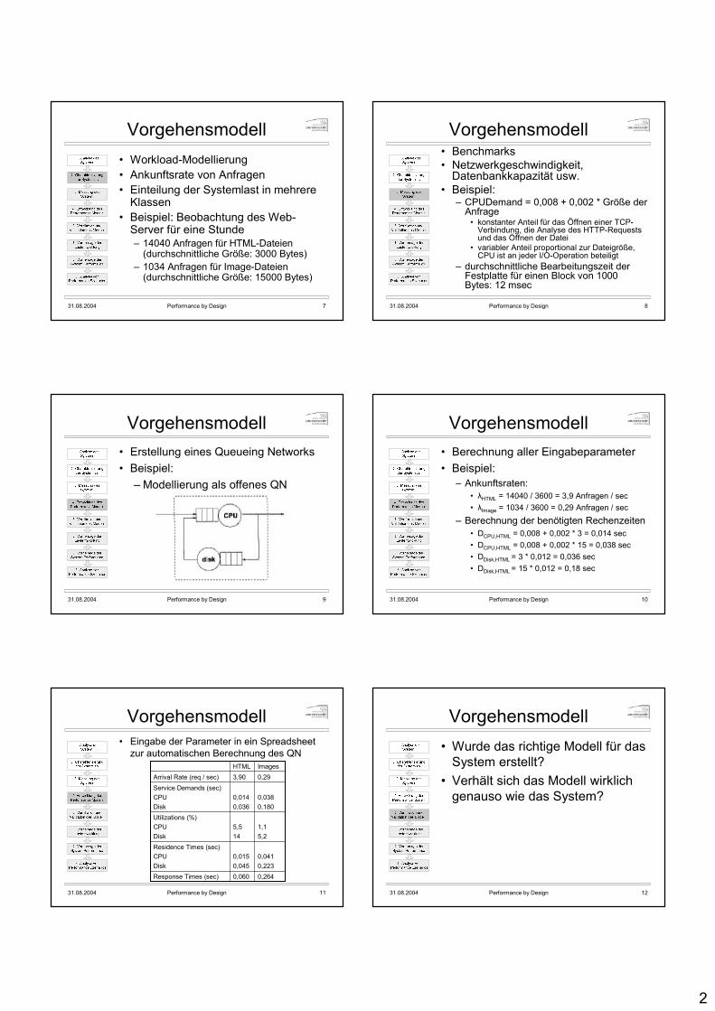
2
31.08.2004 Performance by Design 7
Vorgehensmodell• Workload-Modellierung• Ankunftsrate von Anfragen• Einteilung der Systemlast in mehrere
Klassen• Beispiel: Beobachtung des Web-
Server für eine Stunde – 14040 Anfragen für HTML-Dateien
(durchschnittliche Größe: 3000 Bytes)– 1034 Anfragen für Image-Dateien
(durchschnittliche Größe: 15000 Bytes)
31.08.2004 Performance by Design 8
Vorgehensmodell• Benchmarks• Netzwerkgeschwindigkeit,
Datenbankkapazität usw.• Beispiel:
– CPUDemand = 0,008 + 0,002 * Größe der Anfrage
• konstanter Anteil für das Öffnen einer TCP-Verbindung, die Analyse des HTTP-Requestsund das Öffnen der Datei
• variabler Anteil proportional zur Dateigröße, CPU ist an jeder I/O-Operation beteiligt
– durchschnittliche Bearbeitungszeit der Festplatte für einen Block von 1000 Bytes: 12 msec
31.08.2004 Performance by Design 9
Vorgehensmodell• Erstellung eines Queueing Networks• Beispiel:
– Modellierung als offenes QN
31.08.2004 Performance by Design 10
Vorgehensmodell• Berechnung aller Eingabeparameter• Beispiel:
– Ankunftsraten:• λHTML = 14040 / 3600 = 3,9 Anfragen / sec• λImage = 1034 / 3600 = 0,29 Anfragen / sec
– Berechnung der benötigten Rechenzeiten• DCPU,HTML = 0,008 + 0,002 * 3 = 0,014 sec• DCPU,HTML = 0,008 + 0,002 * 15 = 0,038 sec• DDisk,HTML = 3 * 0,012 = 0,036 sec • DDisk,HTML = 15 * 0,012 = 0,18 sec
31.08.2004 Performance by Design 11
Vorgehensmodell• Eingabe der Parameter in ein Spreadsheet
zur automatischen Berechnung des QN
0,0410,223
0,0150,045
Residence Times (sec)CPUDisk
0,2640,060Response Times (sec)
1,15,2
5,514
Utilizations (%)CPUDisk
0,0380,180
0,0140,036
Service Demands (sec)CPUDisk
0,293,90Arrival Rate (req / sec)ImagesHTML
31.08.2004 Performance by Design 12
Vorgehensmodell• Wurde das richtige Modell für das
System erstellt?• Verhält sich das Modell wirklich
genauso wie das System?

3
31.08.2004 Performance by Design 13
Vorgehensmodell• Statistische Methoden zur
Ermittlung zukünftiger Workloads
• Beispiel: Erhöhung der Systemlast um das 5-fache– Ankunftsraten:
• λHTML = 5 * 3,9 = 19,5 Anfragen / sec• λImage = 5 * 0,29 = 1,45 Anfragen / sec
31.08.2004 Performance by Design 14
Vorgehensmodell• erneute Berechnung des QN• Response Time:
– HTML: 0,93 sec (das 15,5 fache)– Images: 4,61 sec (das 17,5 fache)
• Utilization (disk):– 96 % (vorher: 19,2 %)
�Erreichung der Maximalkapazität bei 5-facher Systemlast
31.08.2004 Performance by Design 15
Vorgehensmodell• Testen verschiedener
Entwurfsalternativen• jeweils Modifikation des QN
• Beispiel: „Wie wirkt sich eine doppelt so schnelle CPU auf die Performance des Systems aus?“
31.08.2004 Performance by Design 16
Vorgehensmodell
in der Übungvorgegeben
31.08.2004 Performance by Design 17
Workload-Modellierung
31.08.2004 Performance by Design 18
Workload-Modellierung• Typen von Workloads
– Natürliche Modelle (Traces, Logs von Webservern)
– Künstliche Modelle• Instruction Mixes• Kernels• Synthetic Programs• Artificial Benchmarks• Drivers
– ausführbare / nicht-ausführbare Modelle

4
31.08.2004 Performance by Design 19
Workload-Modellierung• Systemlast gekennzeichnet durch
– Intensität• Ankunftsrate (z.B. 5 Anfragen / sec)• Anzahl der Clients und Think Times• Anzahl der gleichzeitig ausgeführten Prozesse und
Threads– Service-Anforderungen (Di1, Di2, …, Din),
wobei Dij die Anforderung der Last i an Ressource j ist (z.B. Anfrage i braucht 2 sec auf Ressource j)
31.08.2004 Performance by Design 20
Workload-Modellierung
• Anfragen an ein System– unterschiedliche Anforderungen bzgl. CPU-
Zeit, I/O, Speicherverbrauch, Netzwerkbelastung
– z.B. Abfrage statischer HTML-Seite gegenüber Datenbanktransaktion
– Mittelung der Anforderungen über alle Anfragen -> ungenaue Modellbildung
31.08.2004 Performance by Design 21
Workload-Modellierung�Einteilung aller Anfragen in Klassen
– z.B. einfache, mittlere, komplexe Anfragen• Kriterien
– Ressourcenverbrauch (hoch, niedrig)– Anwendungen (ftp, http)– Dokumenttyp (html, jpg, avi)– Herkunft (.de, .uk, .fr)– …
• bei ähnlichen Objekten: Mittelwertbildung• bei unterschiedlichen Objekten: Cluster-Analyse
31.08.2004 Performance by Design 22
Workload-Modellierung: Cluster-Analyse
• Darstellung der Anfragen eines Beispieldurchlaufs als Punkte in einem mehrdimensionalen Raum (z.B. bzgl. Anzahl der I/O Operationen und CPU-Zeit)
………
10107.6007
1832.8006
1225.4005
………
……...
I/O-Count
CPU-Time
ID
31.08.2004 Performance by Design 23
• Berechnung – Euklidischer Abstands der Punkte– Koordinaten der Mittelpunkte von Clustern
• k-means-Algorithmus1. Setze die Anzahl der Cluster auf k.2. Wähle k Startpunkte als initiale Mittelpunkte.3. Ordne jedem weiteren Punkt den jeweils nahsten
Mittelpunkt zu und berechne dabei den Mittelpunkt neu.4. Wiederhole 3. bis sich kein Mittelpunkt mehr ändert oder
eine maximale Anzahl an Durchläufen erfolgt ist.
Workload-Modellierung: Cluster-Analyse
31.08.2004 Performance by Design 24
Queueing-Networks
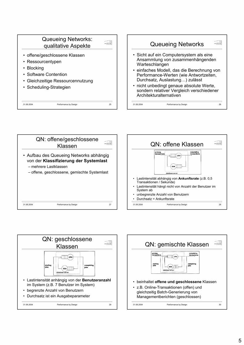
5
31.08.2004 Performance by Design 25
Queueing Networks:qualitative Aspekte
• offene/geschlossene Klassen• Ressourcentypen• Blocking• Software Contention• Gleichzeitige Ressourcennutzung• Scheduling-Strategien
31.08.2004 Performance by Design 26
Queueing Networks• Sicht auf ein Computersystem als eine
Ansammlung von zusammenhängenden Warteschlangen
• einfaches Modell, das die Berechnung von Performance-Werten (wie Antwortzeiten, Durchsatz, Auslastung…) zulässt
• nicht unbedingt genaue absolute Werte, sondern relativer Vergleich verschiedener Architekturalternativen
31.08.2004 Performance by Design 27
QN: offene/geschlossene Klassen
• Aufbau des Queueing Networks abhängig von der Klassifizierung der Systemlast– mehrere Lastklassen– offene, geschlossene, gemischte Systemlast
31.08.2004 Performance by Design 28
QN: offene Klassen
• Lastintensität abhängig von Ankunftsrate (z.B. 0,5 Transaktionen / Sekunde)
• Lastintensität hängt nicht von Anzahl der Benutzer im System ab
• unbegrenzte Anzahl von Benutzern• Durchsatz = Ankunftsrate
31.08.2004 Performance by Design 29
QN: geschlossene Klassen
• Lastintensität anhängig von der Benutzeranzahl im System (z.B. 7 Benutzer im System)
• begrenzte Anzahl von Benutzern• Durchsatz ist ein Ausgabeparameter
31.08.2004 Performance by Design 30
QN: gemischte Klassen
• beinhaltet offene und geschlossene Klassen • z.B. Online-Transaktionen (offen) und
gleichzeitig Batch-Generierung von Managementberichten (geschlossen)
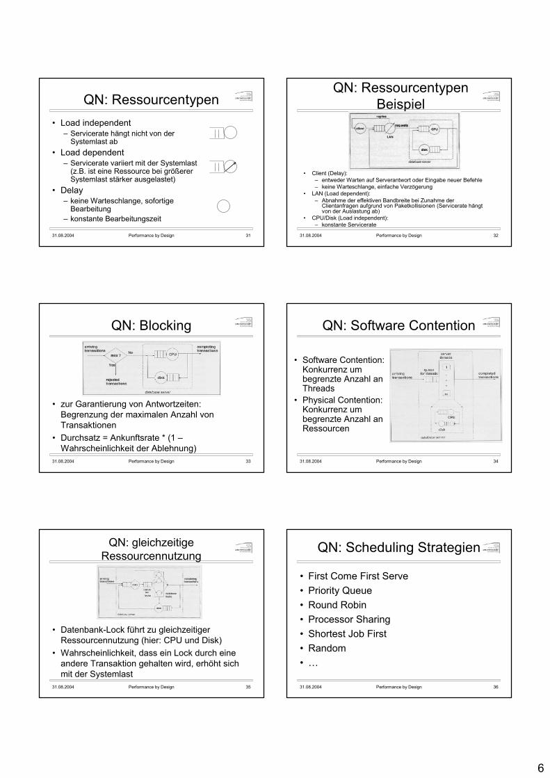
6
31.08.2004 Performance by Design 31
QN: Ressourcentypen• Load independent
– Servicerate hängt nicht von der Systemlast ab
• Load dependent– Servicerate variiert mit der Systemlast
(z.B. ist eine Ressource bei größerer Systemlast stärker ausgelastet)
• Delay– keine Warteschlange, sofortige
Bearbeitung– konstante Bearbeitungszeit
31.08.2004 Performance by Design 32
QN: Ressourcentypen Beispiel
• Client (Delay): – entweder Warten auf Serverantwort oder Eingabe neuer Befehle– keine Warteschlange, einfache Verzögerung
• LAN (Load dependent):– Abnahme der effektiven Bandbreite bei Zunahme der
Clientanfragen aufgrund von Paketkollisionen (Servicerate hängt von der Auslastung ab)
• CPU/Disk (Load independent):– konstante Servicerate
31.08.2004 Performance by Design 33
QN: Blocking
• zur Garantierung von Antwortzeiten: Begrenzung der maximalen Anzahl von Transaktionen
• Durchsatz = Ankunftsrate * (1 –Wahrscheinlichkeit der Ablehnung)
31.08.2004 Performance by Design 34
QN: Software Contention
• Software Contention: Konkurrenz um begrenzte Anzahl an Threads
• Physical Contention: Konkurrenz um begrenzte Anzahl an Ressourcen
31.08.2004 Performance by Design 35
QN: gleichzeitige Ressourcennutzung
• Datenbank-Lock führt zu gleichzeitiger Ressourcennutzung (hier: CPU und Disk)
• Wahrscheinlichkeit, dass ein Lock durch eine andere Transaktion gehalten wird, erhöht sich mit der Systemlast
31.08.2004 Performance by Design 36
QN: Scheduling Strategien
• First Come First Serve• Priority Queue• Round Robin• Processor Sharing• Shortest Job First• Random• …
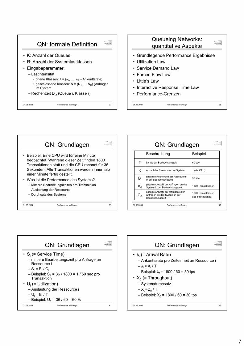
7
31.08.2004 Performance by Design 37
QN: formale Definition
• K: Anzahl der Queues • R: Anzahl der Systemlastklassen• Eingabeparameter:
– Lastintensität• offene Klassen: λ = (λ1, …, λR) (Ankunftsrate)• geschlossene Klassen: N = (N1, … NR) (Anfragen
im System– Rechenzeit Di,r (Queue i, Klasse r)
31.08.2004 Performance by Design 38
Queueing Networks:quantitative Aspekte
• Grundlegende Performance Ergebnisse• Utilization Law• Service Demand Law• Forced Flow Law• Little‘s Law• Interactive Response Time Law• Performance-Grenzen
31.08.2004 Performance by Design 39
QN: Grundlagen• Beispiel: Eine CPU wird für eine Minute
beobachtet. Während dieser Zeit finden 1800 Transaktionen statt und die CPU rechnet für 36 Sekunden. Alle Transaktionen werden innerhalb einer Minute fertig gestellt.
• Was ist die Performance des Systems? – Mittlere Bearbeitungszeiten pro Transaktion– Auslastung der Ressource– Durchsatz des Systems
31.08.2004 Performance by Design 40
QN: GrundlagenBeispielBeschreibung
1800 Transaktionen(job-flow-balance)
gesamte Anzahl der fertiggestelltenAnfragen an das System in der Beobachtungszeit
C0
1800 Transaktionengesamte Anzahl der Anfragen an das System in der BeobachtungszeitA0
36 secgesamte Rechenzeit der Ressource i in der BeobachtungszeitBi
1 (die CPU)Anzahl der Ressourcen im SystemK
60 secLänge der BeobachtungzeitT
31.08.2004 Performance by Design 41
QN: Grundlagen• Si (= Service Time)
– mittlere Bearbeitungszeit pro Anfrage an Ressource i
– Si = Bi / Ci– Beispiel: S1 = 36 / 1800 = 1 / 50 sec pro
Transaktion• Ui (= Utilization)
– Auslastung der Ressource i– Ui = Bi / T– Beispiel: U1 = 36 / 60 = 60 %
31.08.2004 Performance by Design 42
QN: Grundlagen• λi (= Arrival Rate)
– Ankunftsrate pro Zeiteinheit an Ressource i– λi = Ai / T– Beispiel: λ1= 1800 / 60 = 30 tps
• X0 (= Throughput)– Systemdurchsatz– X0=C0 / T– Beispiel: X0 = 1800 / 60 = 30 tps
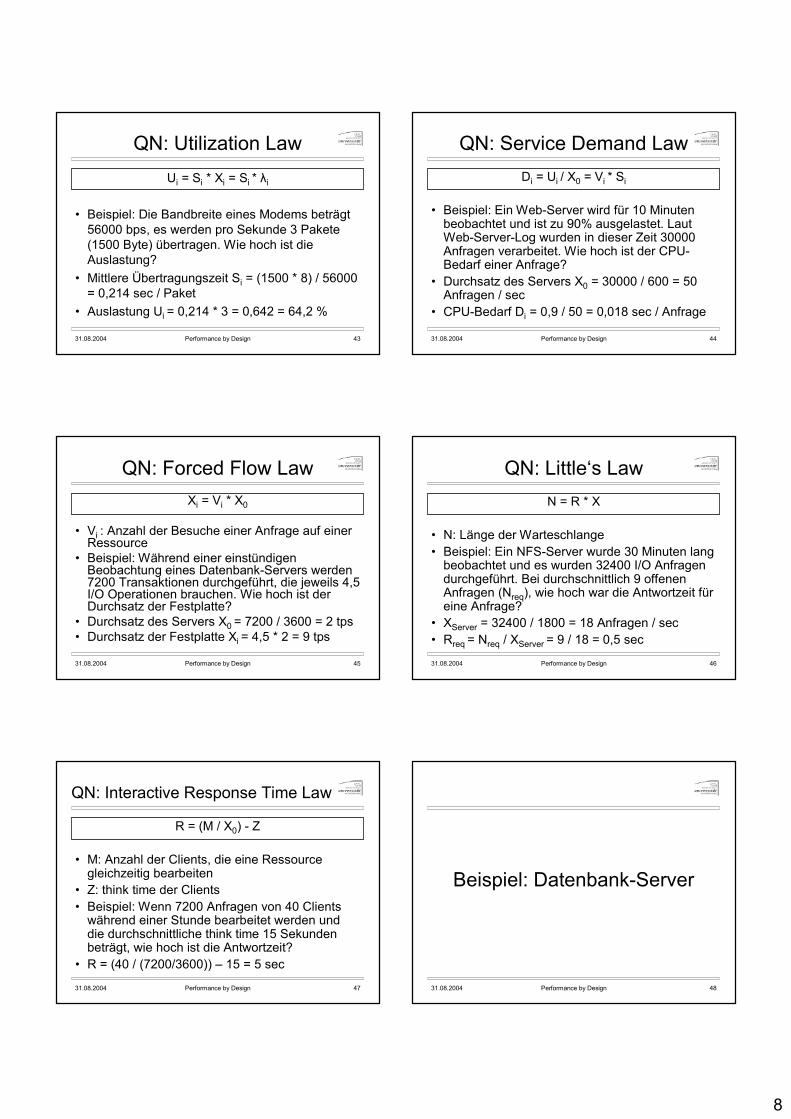
8
31.08.2004 Performance by Design 43
QN: Utilization LawUi = Si * Xi = Si * λi
• Beispiel: Die Bandbreite eines Modems beträgt 56000 bps, es werden pro Sekunde 3 Pakete (1500 Byte) übertragen. Wie hoch ist die Auslastung?
• Mittlere Übertragungszeit Si = (1500 * 8) / 56000 = 0,214 sec / Paket
• Auslastung Ui = 0,214 * 3 = 0,642 = 64,2 %
31.08.2004 Performance by Design 44
QN: Service Demand LawDi = Ui / X0 = Vi * Si
• Beispiel: Ein Web-Server wird für 10 Minuten beobachtet und ist zu 90% ausgelastet. Laut Web-Server-Log wurden in dieser Zeit 30000 Anfragen verarbeitet. Wie hoch ist der CPU-Bedarf einer Anfrage?
• Durchsatz des Servers X0 = 30000 / 600 = 50 Anfragen / sec
• CPU-Bedarf Di = 0,9 / 50 = 0,018 sec / Anfrage
31.08.2004 Performance by Design 45
QN: Forced Flow LawXi = Vi * X0
• Vi : Anzahl der Besuche einer Anfrage auf einer Ressource
• Beispiel: Während einer einstündigen Beobachtung eines Datenbank-Servers werden 7200 Transaktionen durchgeführt, die jeweils 4,5 I/O Operationen brauchen. Wie hoch ist der Durchsatz der Festplatte?
• Durchsatz des Servers X0 = 7200 / 3600 = 2 tps• Durchsatz der Festplatte Xi = 4,5 * 2 = 9 tps
31.08.2004 Performance by Design 46
QN: Little‘s LawN = R * X
• N: Länge der Warteschlange• Beispiel: Ein NFS-Server wurde 30 Minuten lang
beobachtet und es wurden 32400 I/O Anfragen durchgeführt. Bei durchschnittlich 9 offenen Anfragen (Nreq), wie hoch war die Antwortzeit für eine Anfrage?
• XServer = 32400 / 1800 = 18 Anfragen / sec• Rreq = Nreq / XServer = 9 / 18 = 0,5 sec
31.08.2004 Performance by Design 47
QN: Interactive Response Time Law
R = (M / X0) - Z
• M: Anzahl der Clients, die eine Ressource gleichzeitig bearbeiten
• Z: think time der Clients• Beispiel: Wenn 7200 Anfragen von 40 Clients
während einer Stunde bearbeitet werden und die durchschnittliche think time 15 Sekunden beträgt, wie hoch ist die Antwortzeit?
• R = (40 / (7200/3600)) – 15 = 5 sec
31.08.2004 Performance by Design 48
Beispiel: Datenbank-Server
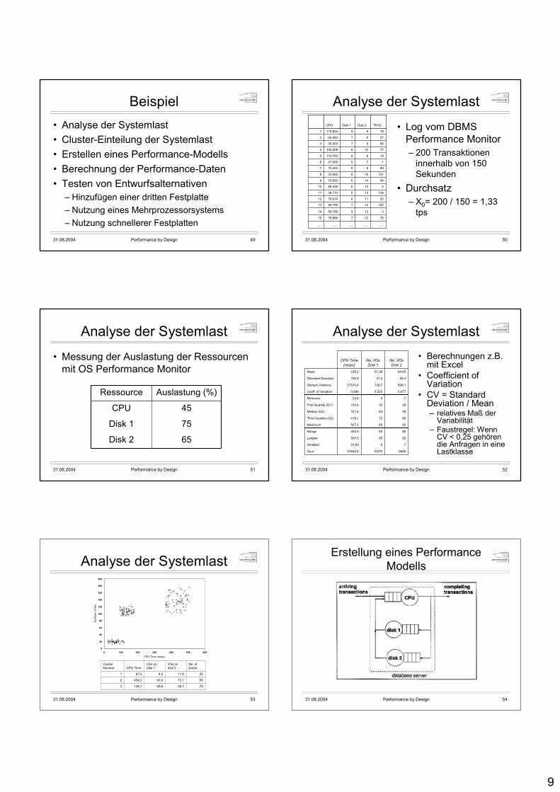
9
31.08.2004 Performance by Design 49
Beispiel• Analyse der Systemlast• Cluster-Einteilung der Systemlast• Erstellen eines Performance-Modells• Berechnung der Performance-Daten• Testen von Entwurfsalternativen
– Hinzufügen einer dritten Festplatte– Nutzung eines Mehrprozessorsystems– Nutzung schnellerer Festplatten
31.08.2004 Performance by Design 50
Analyse der Systemlast
• Log vom DBMS Performance Monitor – 200 Transaktionen
innerhalb von 150 Sekunden
• Durchsatz – X0= 200 / 150 = 1,33
tps7812776,88915
……………
312958,78914
10010759,79513
2011676,01812
13913539,71011
213686,32910
3814670,9009
12115633,8008
998972,4537
17547,9566
1989119,7935
77128104,4094
589735,4033
379764,3832
1899116,8241
TR ID Disk 2Disk 1CPU
31.08.2004 Performance by Design 51
Analyse der Systemlast
• Messung der Auslastung der Ressourcen mit OS Performance Monitor
65Disk 2
75Disk 1
45CPU
Auslastung (%)Ressource
31.08.2004 Performance by Design 52
Analyse der Systemlast
89691027547640,8Sum
7523,60Smallest
9285507,5Largest
8580483,9Range
9285507,5Maximum
6872418,1Third Quartile (Q3)
3963151,6Median (Q2)
2633104,4First Quartile (Q1)
7523,6Minimum
0,6770,5250,696Coeff. of Variation
698,1728,727510,4Sample Variance
26,427,0165,9Standard Deviation
44,8551,38238,2Mean
No. I/Os Disk 2
No. I/Os Disk 1
CPU Time (msec)
• Berechnungen z.B. mit Excel
• Coefficient of Variation
• CV = Standard Deviation / Mean– relatives Maß der
Variabilität– Faustregel: Wenn
CV < 0,25 gehören die Anfragen in eine Lastklasse
31.08.2004 Performance by Design 53
Analyse der Systemlast
0
20
40
60
80
100
120
140
160
180
200
0 100 200 300 400 500 600
CPU Time (msec)
Num
bero
fIO
s
7036,769,8136,13
8073,162,4434,22
5011,08,067,51
No. of points
I/Os on disk 2
I/Os on disk 1CPU Time
Cluster Number
31.08.2004 Performance by Design 54
Erstellung eines Performance Modells

10
31.08.2004 Performance by Design 55
Erstellen eines Performance Modells
• Gegeben:– Ankunftsrate: 1,33 tps (vom DBMS
Performance Monitor)– Auslastung (vom OS Performance Monitor)– Durchsatz (= Ankunftsrate)– Einteilung der Systemlast in drei Klassen
• Gesucht für das QN:– Rechenzeiten für jede Klasse (Service
Demands)
31.08.2004 Performance by Design 56
Erstellen eines Performance Modells
• Service Demand Law– Di,r = Ui,r / X0
– (i ist die Ressource, r die Lastklasse)• Berechnung der Auslastung für die
einzelnen Lastklassen:– Ui,r = Ui * fi,r– fi,r ist ein Faktor, der von Ressourcentyp und
Lastklasse abhängt
31.08.2004 Performance by Design 57
Erstellen eines Performance Modells
• Faktoren für die CPU– fCPU,r = Gesamte CPU-Zeit für Klasse r /
Gesamte CPU Zeit für alle Klassen– fCPU,1 = (67,5 * 50) / 47640,8 = 0,071– fCPU,2 = (434,2 * 80) / 47640,8 = 0,729– fCPU,3 = (136,1 * 70) / 47640,8 = 0,200
31.08.2004 Performance by Design 58
Erstellen eines Performance Modells
• Faktoren für Disk1• fdisk i,r = Gesamte Anzahl an I/Os für Klasse
r / Gesamte Anzahl an I/Os für alle Klassen
• fdisk 1,1 = (8,0 * 50) / 10275 = 0,039• fdisk 1,2 = (62,4 * 80) / 10275 = 0,486• fdisk 1,3 = (69,8 * 70) / 10275 = 0,475
31.08.2004 Performance by Design 59
Erstellen eines Performance Modells
• Faktoren für Disk2• fdisk i,r = Gesamte Anzahl an I/Os für Klasse
r / Gesamte Anzahl an I/Os für alle Klassen
• fdisk 2,1 = (11,0 * 50) / 8969 = 0,061• fdisk 2,2 = (73,1 * 80) / 8969 = 0,652• fdisk 2,3 = (36,7 * 70) / 8969 = 0,287
31.08.2004 Performance by Design 60
Erstellen eines Performance Modells
• Auslastung einer Lastklasse: Ui,r = Ui * fi,r• UCPU,1 = UCPU * fCPU,1 = 0,45 * 0,071 = 0,032• UCPU,2 = UCPU * fCPU,2 = 0,45 * 0,729 = 0,328• UCPU,3 = UCPU * fCPU,3 = 0,45 * 0,200 = 0,090• analog für Disk1 und Disk2
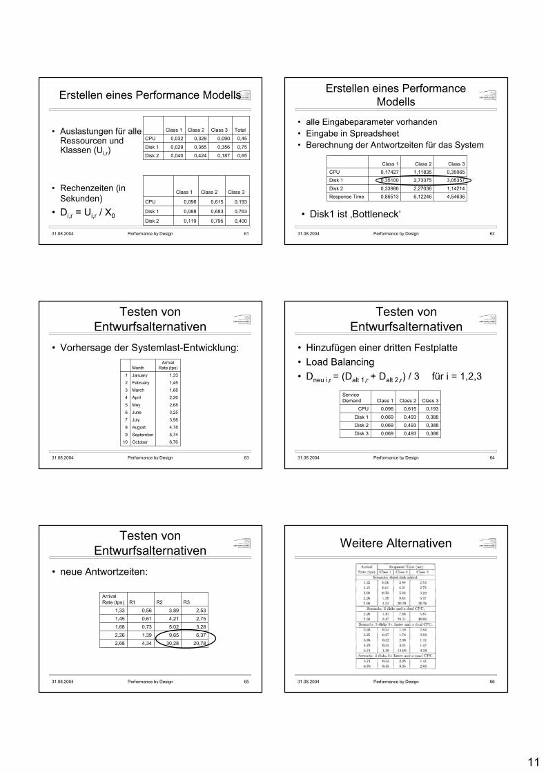
11
31.08.2004 Performance by Design 61
Erstellen eines Performance Modells
• Auslastungen für alle Ressourcen und Klassen (Ui,r) 0,650,1870,4240,040Disk 2
0,750,3560,3650,029Disk 1
0,450,0900,3280,032CPU
TotalClass 3Class 2Class 1
0,4000,7950,119Disk 2
0,7630,6830,088Disk 1
0,1930,6150,096CPU
Class 3Class 2Class 1• Rechenzeiten (in Sekunden)
• Di,r = Ui,r / X0
31.08.2004 Performance by Design 62
Erstellen eines Performance Modells
• alle Eingabeparameter vorhanden• Eingabe in Spreadsheet• Berechnung der Antwortzeiten für das System
4,546366,122460,86513Response Time1,142142,270360,33986Disk 2
3,053572,733750,35100Disk 10,350651,118350,17427CPUClass 3Class 2Class 1
• Disk1 ist ‚Bottleneck‘
31.08.2004 Performance by Design 63
Testen von Entwurfsalternativen
• Vorhersage der Systemlast-Entwicklung:
6,76October10
5,74September9
4,78August8
3,98July7
3,25June6
2,68May5
2,26April4
1,68March3
1,45February2
1,33January1
Arrival Rate (tps)Month
31.08.2004 Performance by Design 64
Testen von Entwurfsalternativen
• Hinzufügen einer dritten Festplatte• Load Balancing• Dneu i,r = (Dalt 1,r + Dalt 2,r) / 3 für i = 1,2,3
0,3880,4930,069Disk 3
0,3880,4930,069Disk 20,3880,4930,069Disk 1
0,1930,6150,096CPUClass 3Class 2Class 1
Service Demand
31.08.2004 Performance by Design 65
Testen von Entwurfsalternativen
• neue Antwortzeiten:
20,7830,284,342,686,379,651,392,26
3,285,020,731,682,754,210,611,45
2,533,890,561,33R3R2R1
Arrival Rate (tps)
31.08.2004 Performance by Design 66
Weitere Alternativen
12
31.08.2004 Performance by Design 67
Fazit: Lernziele der Übung
• Verstehen wie das Vorgehensmodell aufgebaut ist
• Wissen, wie man Workloads in Klassen einteilt
• Wissen, wie man die Eingabeparameter für ein Queueing Network berechnet
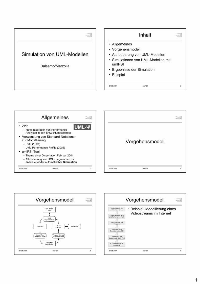
1
Simulation von UML-Modellen
Balsamo/Marzolla
31.08.2004 umlPSI 2
Inhalt
• Allgemeines• Vorgehensmodell• Attributierung von UML-Modellen• Simulationen von UML-Modellen mit
umlPSI• Ergebnisse der Simulation• Beispiel
31.08.2004 umlPSI 3
Allgemeines• Ziel:
– nahe Integration von Performance-Analysen in den Entwicklungsprozess
• Verwendung von Standard-Notationen zur Modellierung– UML (1997)– UML Performance Profile (2002)
• umlPSI-Tool– Thema einer Dissertation Februar 2004– Attributierung von UML-Diagrammen mit
anschließender automatischer Simulation
31.08.2004 umlPSI 4
Vorgehensmodell
31.08.2004 umlPSI 5
Vorgehensmodell
31.08.2004 umlPSI 6
Vorgehensmodell
• Beispiel: Modellierung eines Videostreams im Internet
1. Spezifikation der Architektur mit UML
2. Parametrisierung mit UML Performance Profile
3. Konfiguration der Simulation
4. Automatische Simulation mit umlPSI
5. Feedback der Ergebnisse in CASE-Tool
6. Überarbeitung der Architektur
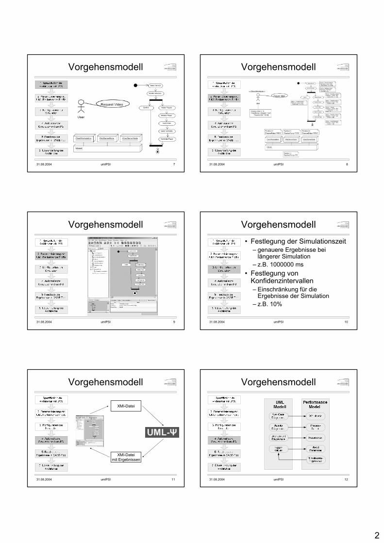
2
31.08.2004 umlPSI 7
Vorgehensmodell
31.08.2004 umlPSI 8
Vorgehensmodell
31.08.2004 umlPSI 9
Vorgehensmodell
31.08.2004 umlPSI 10
Vorgehensmodell• Festlegung der Simulationszeit
– genauere Ergebnisse bei längerer Simulation
– z.B. 1000000 ms• Festlegung von
Konfidenzintervallen– Einschränkung für die
Ergebnisse der Simulation– z.B. 10%
31.08.2004 umlPSI 11
Vorgehensmodell
XMI-Dateimit Ergebnissen
XMI-Datei
31.08.2004 umlPSI 12
Vorgehensmodell

3
31.08.2004 umlPSI 13
Vorgehensmodell
31.08.2004 umlPSI 14
Vorgehensmodell
• Ergebnisse:– Auslastungen von Ressourcen– Durchsatz von Ressourcen– Mittlere Ausführungszeiten für
Aktionen und Use-Cases• spezielle Attribute zur
Speicherung der Ergebnisse im UML-Modell
31.08.2004 umlPSI 15
Vorgehensmodell
31.08.2004 umlPSI 16
Vorgehensmodell
• Ergebnisse:
• Internet-Ressource am stärksten belastet (~76%)
• Testen verschiedener Entwurfsalternativen
31.08.2004 umlPSI 17
Attributierung von UML-Diagrammen
UML Performance Profile
31.08.2004 umlPSI 18
Erweiterungsmechanismen für UML
• Stereotypes– Definition von Subklassen für existierenden Metamodell-
Elemente– Gleiche Struktur wie Original, Erweiterungen– graphische Repräsentierung: <<stereotype>>
• Tagged-Values– Attribute für Modell-Elemente– Beispiel: PAhost = „Workstation“
• Constraints– Einschränkungen für ein Attribut– Beispiel: PArespTime < 1.5
• Profile– Paket mit speziell für eine Domäne angepassten Modell-
Elementen– Definition von Stereotypes, Tagged Values und Constraints
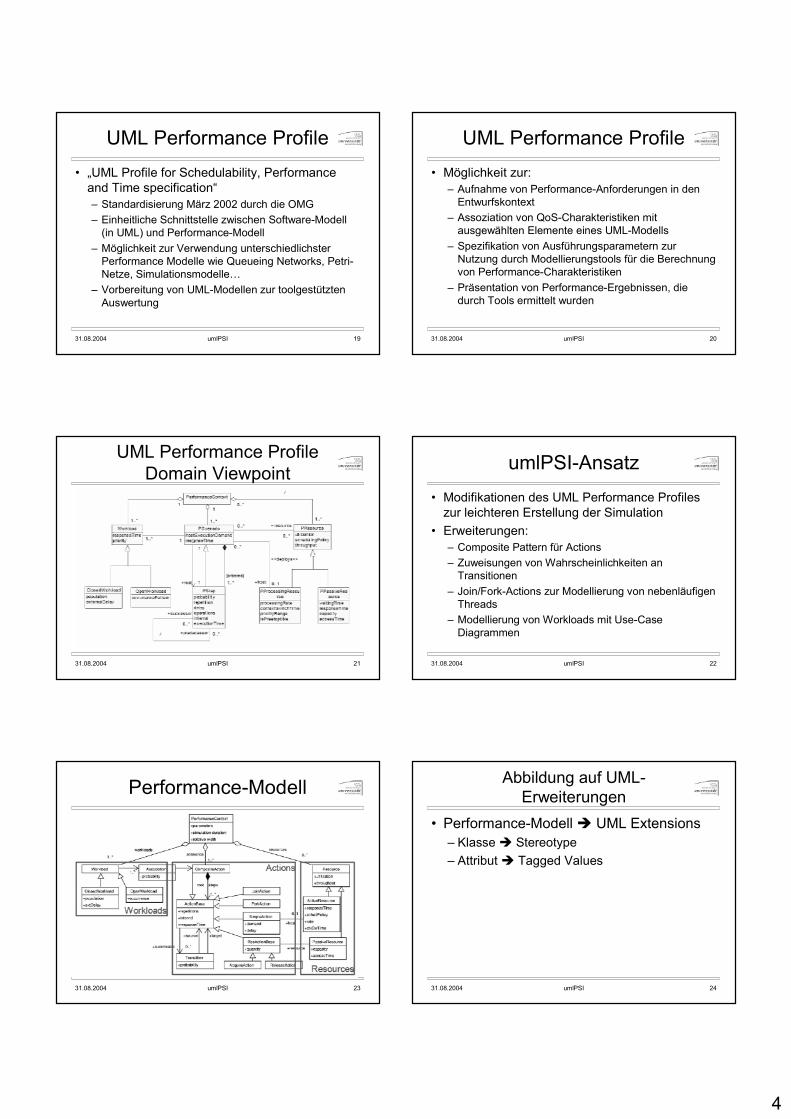
4
31.08.2004 umlPSI 19
UML Performance Profile• „UML Profile for Schedulability, Performance
and Time specification“– Standardisierung März 2002 durch die OMG– Einheitliche Schnittstelle zwischen Software-Modell
(in UML) und Performance-Modell– Möglichkeit zur Verwendung unterschiedlichster
Performance Modelle wie Queueing Networks, Petri-Netze, Simulationsmodelle…
– Vorbereitung von UML-Modellen zur toolgestützten Auswertung
31.08.2004 umlPSI 20
UML Performance Profile• Möglichkeit zur:
– Aufnahme von Performance-Anforderungen in den Entwurfskontext
– Assoziation von QoS-Charakteristiken mit ausgewählten Elemente eines UML-Modells
– Spezifikation von Ausführungsparametern zur Nutzung durch Modellierungstools für die Berechnung von Performance-Charakteristiken
– Präsentation von Performance-Ergebnissen, die durch Tools ermittelt wurden
31.08.2004 umlPSI 21
UML Performance ProfileDomain Viewpoint
31.08.2004 umlPSI 22
umlPSI-Ansatz• Modifikationen des UML Performance Profiles
zur leichteren Erstellung der Simulation• Erweiterungen:
– Composite Pattern für Actions– Zuweisungen von Wahrscheinlichkeiten an
Transitionen– Join/Fork-Actions zur Modellierung von nebenläufigen
Threads– Modellierung von Workloads mit Use-Case
Diagrammen
31.08.2004 umlPSI 23
Performance-Modell
31.08.2004 umlPSI 24
Abbildung auf UML-Erweiterungen
• Performance-Modell � UML Extensions– Klasse � Stereotype– Attribut � Tagged Values

5
31.08.2004 umlPSI 25
Modellierung von Workloads: offene Systemlastklassen
Wahrscheinlichkeit, dass eine Transition genommen wirdPAprob
Ankunftsrate für Anfragen an das SystemPAoccurrence
31.08.2004 umlPSI 26
Modellierung von Workloads: geschlossene Systemlastklassen
Wahrscheinlichkeit, dass eine Transition genommen wirdPAprob
externe Verzögerung zwischen zwei Anfragen (think time)PAextDelayAnzahl der Anfragen im SystemPApopulation
31.08.2004 umlPSI 27
Modellierung von Szenarien: einfache Zustände
Service Demand: die benötigte Rechenzeit für diesen SchrittPAdemand
Anzahl der WiederholungenPArepIntervallzeit zwischen zwei WiederholungenPAinterval
Ressource, auf der dieser Schritt ausgeführt wird (diese muss im Deployment-Diagramm enthalten sein)
PAhost
Antwortzeit für diesen Schritt (berechnet umlPSI)PArespTime
Verzögerung (z.B. für eine Benutzerinteraktion)PAdelay
31.08.2004 umlPSI 28
Modellierung von Szenarien: Akquirierung von passiven Ressourcen
Aquire/Release<<GRMaquire>> / <<GRMrelease>>
PAresource = „Memory“PAquantity = [„assm“, „dist“, [„constant“, 2]]
Ressource, die besetzt oder freigegeben wirdPAresource
Anzahl der Ressourcen, die besetzt oder freigegeben werden PAquantity
31.08.2004 umlPSI 29
Modellierung von Ressourcen: Aktive Ressourcen
Workstation
<<PAhost>>
PAschedPolicy = „FIFO“PActxSwT = [„constant“, 0,1]PArate = 2.0PAutilization = @xx@PAthroughput = @xx@
Scheduling-Strategie: (FIFO, LIFO, PS(=Processor Sharing))PAschedPolicyZeit für eine Kontextwechsel (nur falls Scheduling-Strategie PS)PActxSwT
Rechengeschwindigkeit im Verhältnis zum Referenz-Prozessor (benötigt 1 sec Rechenzeit für 1 sec Service Demand)
PArate
Durchsatz der Ressource (berechnet umlPSI)PAthroughput
Auslastung der Ressource (berechnet umlPSI)PAutilization
31.08.2004 umlPSI 30
Modellierung von Ressourcen: Passive Ressourcen
maximale Anzahl von InstanzenPAcapacity
physikalische Zugriffszeit, Zeit zwischen Besetzung der Ressource und ihrer Einsatzfähigkeit (Freigabe verbraucht keine Zeit)
PAaxTime
Durchsatz der Ressource (berechnet umlPSI)PAthroughputAuslastung der Ressource (berechnet umlPSI)PAutilization
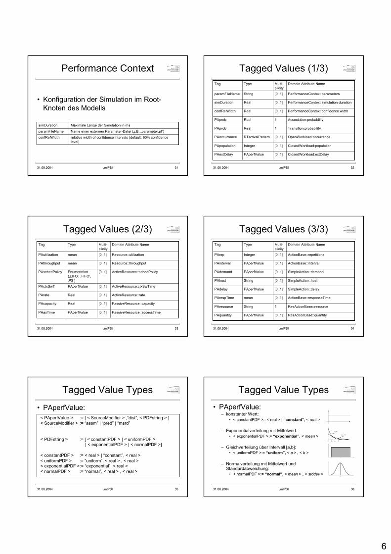
6
31.08.2004 umlPSI 31
Performance Context
• Konfiguration der Simulation im Root-Knoten des Modells
Maximale Länge der Simulation in mssimDuration
Name einer externen Parameter-Datei (z.B. „parameter.pl“)paramFileName
relative width of confidence intervals (default: 90% confidencelevel)
confRelWidth
31.08.2004 umlPSI 32
Tagged Values (1/3)
ClosedWorkload:extDelay[0..1]PAperfValuePAextDelay
ClosedWorkload:population[0..1]IntegerPApopulation
OpenWorkload:occurrence[0..1]RTarrivalPatternPAoccurrence
Transition:probability1RealPAprob
Association:probability1RealPAprob
PerformanceContext:confidence width[0..1]RealconfRelWidth
PerformanceContext:simulation duration[0..1]RealsimDuration
PerformanceContext:parameters[0..1]StringparamFileName
Domain Attribute NameMulti-plicity
TypeTag
31.08.2004 umlPSI 33
Tagged Values (2/3)
PassiveResource::accessTime[0..1]PAperfValuePAaxTime
PassiveResource::capacity[0..1]RealPAcapacity
ActiveResource::rate[0..1]RealPArate
ActiveResource:ctxSwTime[0..1]PAperfValuePActxSwT
ActiveResource::schedPolicy[0..1]Enumeration{‚LIFO‘, ‚FIFO‘, ‚PS‘}
PAschedPolicy
Resource::throughput[0..1]meanPAthroughput
Resource::utilization[0..1]meanPAutilization
Domain Attribute NameMulti-plicity
TypeTag
31.08.2004 umlPSI 34
Tagged Values (3/3)
ResActionBase::resource1StringPAresource
ResActionBase::quantity[0..1]PAperfValuePAquantity
ActionBase::responseTime[0..1]meanPArespTime
SimpleAction::delay[0..1]PAperfValuePAdelay
SimpleAction::host[0..1]StringPAhost
SimpleAction::demand[0..1]PAperfValuePAdemand
ActionBase::interval[0..1]PAperfValuePAinterval
ActionBase::repetitions[0..1]IntegerPArep
Domain Attribute NameMulti-plicity
TypeTag
31.08.2004 umlPSI 35
Tagged Value Types
< PAperfValue > := [ < SourceModifier > ,“dist”, < PDFstring > ]< SourceModifier > := “assm” | “pred” | “msrd”
< PDFstring > := [ < constantPDF > | < uniformPDF >| < exponentialPDF > | < normalPDF >]
< constantPDF > := < real > | “constant”, < real >< uniformPDF > := “uniform”, < real > , < real >< exponentialPDF >:= “exponential”, < real >< normalPDF > := “normal”, < real > , < real >
• PAperfValue:
31.08.2004 umlPSI 36
Tagged Value Types• PAperfValue:
– konstanter Wert: • < constantPDF >:=< real > | “constant”, < real >
– Exponentialverteilung mit Mittelwert: • < exponentialPDF >:= “exponential”, < mean >
– Gleichverteilung über Intervall [a,b]: • < uniformPDF >:= “uniform”, < a > , < b >
– Normalverteilung mit Mittelwert und Standardabweichung:
• < normalPDF >:= “normal”, < mean > , < stddev >
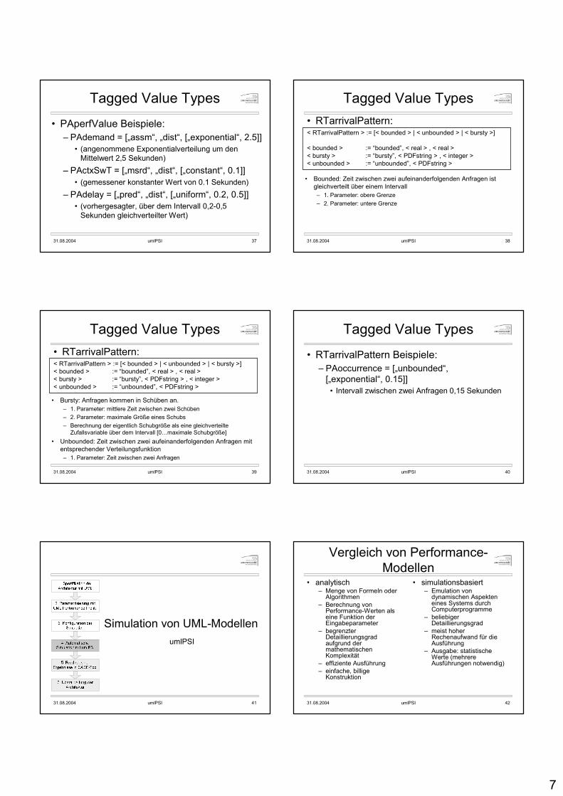
7
31.08.2004 umlPSI 37
Tagged Value Types
• PAperfValue Beispiele: – PAdemand = [„assm“, „dist“, [„exponential“, 2.5]]
• (angenommene Exponentialverteilung um den Mittelwert 2,5 Sekunden)
– PActxSwT = [„msrd“, „dist“, [„constant“, 0.1]]• (gemessener konstanter Wert von 0.1 Sekunden)
– PAdelay = [„pred“, „dist“, [„uniform“, 0.2, 0.5]]• (vorhergesagter, über dem Intervall 0,2-0,5
Sekunden gleichverteilter Wert)
31.08.2004 umlPSI 38
Tagged Value Types• RTarrivalPattern:< RTarrivalPattern > := [< bounded > | < unbounded > | < bursty >]
< bounded > := “bounded”, < real > , < real >< bursty > := “bursty”, < PDFstring > , < integer >< unbounded > := “unbounded”, < PDFstring >
• Bounded: Zeit zwischen zwei aufeinanderfolgenden Anfragen ist gleichverteilt über einem Intervall– 1. Parameter: obere Grenze– 2. Parameter: untere Grenze
31.08.2004 umlPSI 39
Tagged Value Types• RTarrivalPattern:< RTarrivalPattern > := [< bounded > | < unbounded > | < bursty >]< bounded > := “bounded”, < real > , < real >< bursty > := “bursty”, < PDFstring > , < integer >< unbounded > := “unbounded”, < PDFstring >
• Bursty: Anfragen kommen in Schüben an. – 1. Parameter: mittlere Zeit zwischen zwei Schüben– 2. Parameter: maximale Größe eines Schubs– Berechnung der eigentlich Schubgröße als eine gleichverteilte
Zufallsvariable über dem Intervall [0…maximale Schubgröße]• Unbounded: Zeit zwischen zwei aufeinanderfolgenden Anfragen mit
entsprechender Verteilungsfunktion– 1. Parameter: Zeit zwischen zwei Anfragen
31.08.2004 umlPSI 40
Tagged Value Types
• RTarrivalPattern Beispiele:– PAoccurrence = [„unbounded“,
[„exponential“, 0.15]]• Intervall zwischen zwei Anfragen 0,15 Sekunden
31.08.2004 umlPSI 41
Simulation von UML-ModellenumlPSI
31.08.2004 umlPSI 42
Vergleich von Performance-Modellen
• analytisch– Menge von Formeln oder
Algorithmen– Berechnung von
Performance-Werten als eine Funktion der Eingabeparameter
– begrenzter Detaillierungsgrad aufgrund der mathematischen Komplexität
– effiziente Ausführung– einfache, billige
Konstruktion
• simulationsbasiert– Emulation von
dynamischen Aspekten eines Systems durch Computerprogramme
– beliebiger Detaillierungsgrad
– meist hoher Rechenaufwand für die Ausführung
– Ausgabe: statistische Werte (mehrere Ausführungen notwendig)
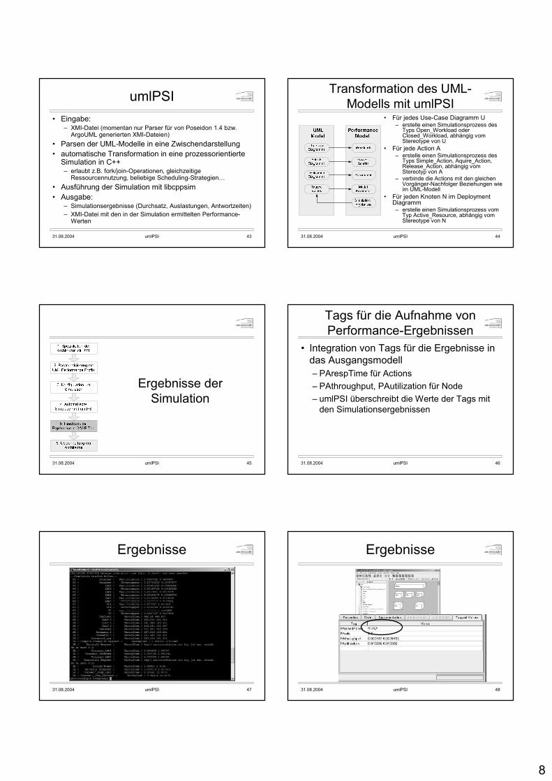
8
31.08.2004 umlPSI 43
umlPSI• Eingabe:
– XMI-Datei (momentan nur Parser für von Poseidon 1.4 bzw. ArgoUML generierten XMI-Dateien)
• Parsen der UML-Modelle in eine Zwischendarstellung• automatische Transformation in eine prozessorientierte
Simulation in C++– erlaubt z.B. fork/join-Operationen, gleichzeitige
Ressourcennutzung, beliebige Scheduling-Strategien…• Ausführung der Simulation mit libcppsim• Ausgabe:
– Simulationsergebnisse (Durchsatz, Auslastungen, Antwortzeiten)– XMI-Datei mit den in der Simulation ermittelten Performance-
Werten
31.08.2004 umlPSI 44
Transformation des UML-Modells mit umlPSI
• Für jedes Use-Case Diagramm U– erstelle einen Simulationsprozess des
Typs Open_Workload oder Closed_Workload, abhängig vom Stereotype von U
• Für jede Action A– erstelle einen Simulationsprozess des
Typs Simple_Action, Aquire_Action, Release_Action, abhängig vom Stereotyp von A
– verbinde die Actions mit den gleichen Vorgänger-Nachfolger Beziehungen wie im UML-Modell
• Für jeden Knoten N im DeploymentDiagramm– erstelle einen Simulationsprozess vom
Typ Active_Resource, abhängig vom Stereotype von N
31.08.2004 umlPSI 45
Ergebnisse der Simulation
31.08.2004 umlPSI 46
Tags für die Aufnahme von Performance-Ergebnissen
• Integration von Tags für die Ergebnisse in das Ausgangsmodell– PArespTime für Actions– PAthroughput, PAutilization für Node– umlPSI überschreibt die Werte der Tags mit
den Simulationsergebnissen
31.08.2004 umlPSI 47
Ergebnisse
31.08.2004 umlPSI 48
Ergebnisse
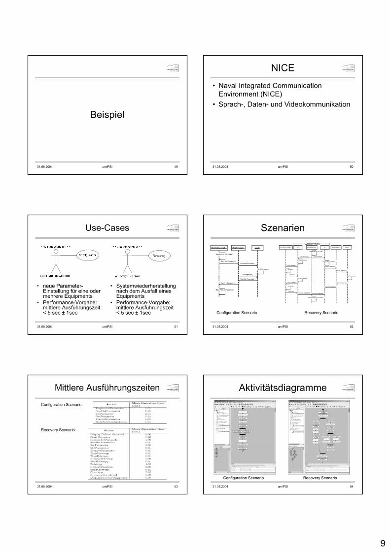
9
31.08.2004 umlPSI 49
Beispiel
31.08.2004 umlPSI 50
NICE
• Naval Integrated CommunicationEnvironment (NICE)
• Sprach-, Daten- und Videokommunikation
31.08.2004 umlPSI 51
Use-Cases
• neue Parameter-Einstellung für eine oder mehrere Equipments
• Performance-Vorgabe: mittlere Ausführungszeit < 5 sec ± 1sec
• Systemwiederherstellung nach dem Ausfall eines Equipments
• Performance-Vorgabe: mittlere Ausführungszeit < 5 sec ± 1sec
31.08.2004 umlPSI 52
Szenarien
Configuration Scenario Recovery Scenario
31.08.2004 umlPSI 53
Mittlere Ausführungszeiten
Configuration Scenario:
Recovery Scenario:
31.08.2004 umlPSI 54
Aktivitätsdiagramme
Recovery ScenarioConfiguration Scenario
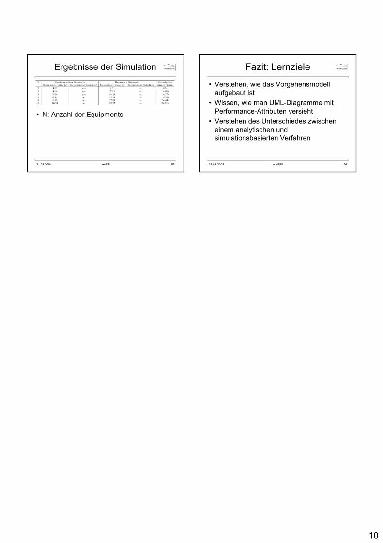
10
31.08.2004 umlPSI 55
Ergebnisse der Simulation
• N: Anzahl der Equipments
31.08.2004 umlPSI 56
Fazit: Lernziele
• Verstehen, wie das Vorgehensmodell aufgebaut ist
• Wissen, wie man UML-Diagramme mit Performance-Attributen versieht
• Verstehen des Unterschiedes zwischen einem analytischen und simulationsbasierten Verfahren
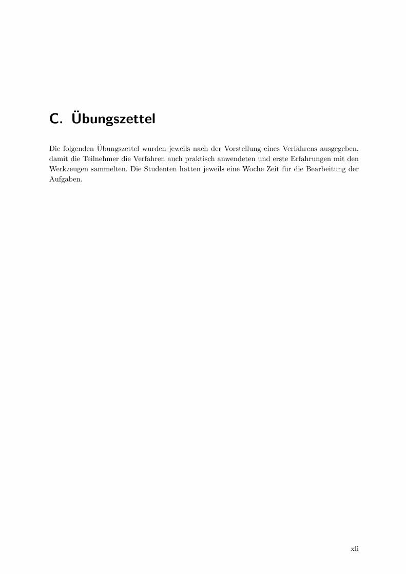
C. Ubungszettel
Die folgenden Ubungszettel wurden jeweils nach der Vorstellung eines Verfahrens ausgegeben,damit die Teilnehmer die Verfahren auch praktisch anwendeten und erste Erfahrungen mit denWerkzeugen sammelten. Die Studenten hatten jeweils eine Woche Zeit fur die Bearbeitung derAufgaben.
xli
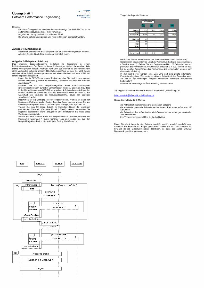
Übungsblatt 1 Software Performance Engineering
Hinweise: • Für diese Übung wird ein Windows-Rechner benötigt. Das SPE-ED-Tool ist für
andere Betriebssysteme leider nicht verfügbar. • Abgabe der Lösung per Mail (s.u.) bis zum 22.06. • Die Übung soll als Einzelperson und nicht in Gruppen bearbeitet werden.
Aufgabe 1 (Einarbeitung) • Installieren Sie das SPE-ED-Tool (kann von Stud-IP heruntergeladen werden). • Arbeiten Sie die „Quick-Start-Anleitung“ gründlich durch.
Aufgabe 2 (Beispielarchitektur) Das folgende Sequenzdiagramm modelliert die Recherche in einem Bibliotheksverzeichnis. Der Benutzer kann Suchanfragen stellen, die an das lokale DBMS weitergeleitet werden. Alternativ kann über das Internet die Zentraldatenbank eines Verbundes mehrerer anderer Bibliotheken abgefragt werden. Der Web-Server und das lokale DBMS werden gemeinsam auf einem Rechner mit einer CPU und einer Festplatten ausgeführt.
• Legen Sie in SPE-ED ein neues Projekt an, das Sie nach ihrem eigenen Namen benennen („Markus Mustermann“). Erstellen Sie darin ein Szenario „bookSearch“.
• Erstellen Sie für das Sequenzdiagramm einen Execution-Graphen (Synchronisation kann zunächst vernachlässigt werden). Beachten Sie, dass in der Demo-Version von SPE-ED nur maximal 4 Subgraphen erstellt werden können. Gehen Sie davon aus, dass die Suche nach einem Buchtitel 10 mal wiederholt wird (Schleife im Sequenzdiagramm), bevor der Benutzer „viewDetails“ aufruft.
• Bestimmen Sie die Software Resource Requirements. Wählen Sie dazu den Menüpunkt (Software Model / Assign Template Spec) aus und weisen Sie aus den Beispiel-Projekten (Button „Show All“) die Vorlage „Distr sys spec“ zu.
• Tragen Sie nun für jeden Schritt im Execution Graph die jeweiligen geschätzten Werte ein (Software Model / Specify values). Versuchen Sie möglichst realistische Werte anzugeben und modifizieren Sie dazu diese Werte ggf. nachträglich.
• Weisen Sie die Computer Resource Requirements zu. Wählen Sie dazu den Menüpunkt (Overhead / Facility template) aus und weisen Sie aus den Beispiel-Projekten (Button „Show All“) die Facility „WebServer“ zu.
• Tragen Sie folgende Werte ein:
• Berechnen Sie die Antwortzeiten des Szenarios (No Contention-Solution). • Spezifizieren Sie den Service-Level der Architektur (Software Execution Model
/ Service level…). Geben Sie als Performance-Ziel 120 Sekunden an und probieren Sie verschiedene Ankunftsraten zwischen 0-1 aus. Stellen Sie fest, bis zu welcher Ankunftsrate das Performance-Ziel eingehalten werden kann (Contention-Solution).
• In den Web-Server werden eine Dual-CPU und eine zweite (identische) Festplatte eingebaut. Wie verändert sich die Antwortzeit des Szenarios, wenn Sie die in der vorherigen Aufgabe ermitteltete maximale Ankunftsrate beibehalten?
• Machen Sie Vorschläge zur Überarbeitung der Architektur.
Zur Abgabe: Schreiben Sie eine E-Mail mit dem Betreff „SPE-Übung“ an [email protected]
Geben Sie im Body der E-Mail an: • die Antwortzeit des Szenarios (No Contention-Solution), • die ermittelte maximale Ankunftsrate bei einem Performance-Ziel von 120
Sekunden, • die Antwortzeit des aufgerüsteten Web-Servers bei der vorherigen maximalen
Ankunftsrate und • ihre Verbesserungsvorschläge für die Architektur.
Fügen Sie als Anhang die vier Dateien (spedb0, spedb1, spedb2, spedb3) hinzu, nachdem Sie Szenario und Projekt gespeichert haben. (In der Demo-Version von SPE-ED ist die Exportfunktionalität deaktiviert, so dass die ganze SPE-ED-Datenbank geschickt werden muss.)
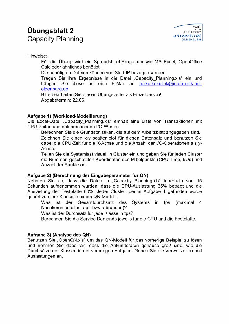
Übungsblatt 2 Capacity Planning
Hinweise: • Für die Übung wird ein Spreadsheet-Programm wie MS Excel, OpenOffice
Calc oder ähnliches benötigt. • Die benötigten Dateien können von Stud-IP bezogen werden. • Tragen Sie ihre Ergebnisse in die Datei „Capacity_Planning.xls“ ein und
hängen Sie diese an eine E-Mail an [email protected]
• Bitte bearbeiten Sie diesen Übungszettel als Einzelperson! • Abgabetermin: 22.06.
Aufgabe 1) (Workload-Modellierung) Die Excel-Datei „Capacity_Planning.xls“ enthält eine Liste von Transaktionen mit CPU-Zeiten und entsprechenden I/O-Werten.
• Berechnen Sie die Grundstatistiken, die auf dem Arbeitsblatt angegeben sind. • Zeichnen Sie einen x-y scatter plot für diesen Datensatz und benutzen Sie
dabei die CPU-Zeit für die X-Achse und die Anzahl der I/O-Operationen als y-Achse.
• Teilen Sie die Systemlast visuell in Cluster ein und geben Sie für jeden Cluster die Nummer, geschätzten Koordinaten des Mittelpunkts (CPU Time, I/Os) und Anzahl der Punkte an.
Aufgabe 2) (Berechnung der Eingabeparameter für QN) Nehmen Sie an, dass die Daten in „Capacity_Planning.xls“ innerhalb von 15 Sekunden aufgenommen wurden, dass die CPU-Auslastung 35% beträgt und die Auslastung der Festplatte 80%. Jeder Cluster, der in Aufgabe 1 gefunden wurde gehört zu einer Klasse in einem QN-Modell.
• Was ist der Gesamtdurchsatz des Systems in tps (maximal 4 Nachkommastellen, auf- bzw. abrunden)?
• Was ist der Durchsatz für jede Klasse in tps? • Berechnen Sie die Service Demands jeweils für die CPU und die Festplatte.
Aufgabe 3) (Analyse des QN) Benutzen Sie „OpenQN.xls“ um das QN-Modell für das vorherige Beispiel zu lösen und nehmen Sie dabei an, dass die Ankunftsraten genauso groß sind, wie die Durchsätze der Klassen in der vorherigen Aufgabe. Geben Sie die Verweilzeiten und Auslastungen an.
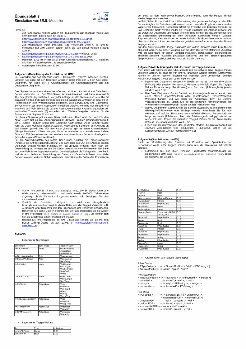
Übungsblatt 3 Simulation von UML-Modellen Hinweise:
• Zur Performance-Analyse werden die Tools umlPSI und libcppsim (beide Unix only) benötigt (gibt es auch auf StudIP).
• http://www.dsi.unive.it/~marzolla/software/libcppsim-0.2.2.tar.gz • http://www.dsi.unive.it/~marzolla/software/umlPSI-0.5.1.tar.gz • Zur Modellierung muss Poseidon 1.41 verwendet werden, da umlPSI
momentan nur XMI-Dateien parsen kann, die von dieser Version erzeugt wurden.
• ftp://ftp.gentleware.org/1.4.1/PoseidonCE-1.4.1.zip (Windows, Linux) • ftp://ftp.gentleware.org/1.4.1/PoseidonCE-1.4.1.dmg.tar.gz (Mac) • Poseidon 1.4.1 ist in der ARBI unter /usr/local/java/poseidon1.4.1 installiert
und kann mit startPoseidon141 gestartet werden. • Abgabe per E-Mail bis zum 22.06.
Aufgabe 1) (Modellierung der Architektur mit UML) Im Folgenden soll das Szenario eines E-Commerce Systems modelliert werden. Erstellen Sie dazu mit den folgenden Angaben unter Poseidon 1.4 ein Use Case-Diagramm, für jeden der 4 Anwendungfälle ein Aktivitätsdiagramm und ein Deployment Diagramm. Das System besteht aus einem Web-Server, der über LAN mit einem Datenbank-Server verbunden ist. Der Web-Server ist multi-threaded und kann maximal 5 Threads gleichzeitig ausführen. Vor jeder Anfrage an das System muss ein Thread akquiriert werden. Falls alle Threads belegt sind, werden die Anfragen in einer FIFO-Reihenfolge in eine Warteschlange eingereiht. Web-Server, LAN und Datenbank-Server können als aktive Ressourcen modelliert werden, während der Thread-Pool innerhalb des Web-Servers als passive Ressource mit einer Kapazität äquivalent zur maximalen Threadanzahl (5) modelliert wird. Weitere Vorgaben müssen für die Ressourcen nicht gemacht werden. Für dieses Szenario gibt es zwei Benutzerklassen: „User“ und „Service“. Für den Aktor „User“ gibt es drei Anwendungsfälle: „Browse Product“ (Wahrscheinlichkeit: 80%), „Select Product“ (10%) und „Checkout Cart“ (10%). Diese Benutzerklasse kann als Open Workload modelliert werden, wobei alle 60 Sekunden eine Anfrage an das System gestellt wird. Für den Aktor „Service“ gibt es einen Anwendungsfall („Purge Database“). Dieser Vorgang findet in Intervallen von jeweils einer halben Stunde (1800 Sekunden) statt und wird nur von einem festen Benutzer durchgeführt (Modellierung als Closed Workload). Für alle Anwendungsfälle des Aktors „User“ muss zunächst ein Thread akquiriert (Action1), die Anfrage geparst (Action2) und dann über das LAN eine Anfrage an den DB-Server gestellt werden (Action3). Im Fall „Browse Product“ kann nach der Übermittlung der Anfrage an den DB-Server bereits mit dem Formatieren der Seite auf dem Web-Server begonnen werden. Gleichzeitig läuft die Abfrage der Datenbank und die anschließende Übermittlung der Daten vom Datenbank-Server zum Web-Server. In einem weiteren Schritt wird nach Übermittlung der Daten das Formatieren
der Seite auf dem Web-Server beendet. Anschließend kann der belegte Thread wieder freigegeben werden. Im Fall „Select Product“ wird nach Übermittlung der geparsten Anfrage an den DB-Server lediglich die Datenbank aktualisiert, danach wird das Ergebnis zurück an den Web-Server transferiert. Schließlich erfolgt die Freigabe des belegten Threads. Im Fall „Checkout Cart“ werden wieder ein Thread eingeholt, die Anfrage geparst und die Daten zur Datenbank übertragen. Anschließend können die Bezahlmethode und die Bestelldaten gleichzeitig auf dem DB-Server kontrolliert werden (Validate Payment einmal, Validate Order für jeden Artikel). Die Ergebnisse werden wieder über das LAN zurück an den Web-Server geliefert, worauf im Anschluss der Thread freigegeben wird. Für den Anwendungsfall „Purge Database“ des Aktors „Service“ muss kein Thread akquiriert werden, da dieser Vorgang nur auf dem DB-Server stattfindet. Zunächst wird die Datenbank für diesen Vorgang initialisiert, dann werden gleichzeitig die aktuellen Sessions invalidiert (Invalidate Sessions) und die Tabellen gesäubert (Empty Charts). Anschließend folgt noch ein Schritt Cleanup. Aufgabe 2) (Attributierung der UML-Elemente mit Tagged-Values) Nun sollen alle Elemente des UML-Modells mit Stereotypes bzw. Tagged-Values versehen werden, so dass sie von umlPSI analysiert werden können. Stereotypes können im unteren rechten Abschnitt von Poseidon unter „Properties“ definiert werden. Für Tagged Values gibt es ein eigenes Tab.
• Deployment Diagramm: Geben Sie jeweils an, ob es sich um eine aktive (PAhost) oder passive (PAresource) Ressource handelt. Fügen Sie Tagged Values für Auslastung (PAutilization) und Durchsatz (PAthroughput) jeweils mit dem Wert 0 ein.
• Use Case Diagramm: Geben Sie bei den Aktoren jeweils an, ob es sich um einen offenen (OpenWorkload) oder geschlossenen (ClosedWorkload) Workload handelt und wie hoch die Ankunftrate bzw. die externe Verzögerungsrate ist. Legen Sie für die einzelnen Anwendungsfälle die Wahrscheinlichkeiten (PAprob) jeweils an den Transitionen fest.
• Activity Diagramme: Geben Sie für die Schritte jeweils an, ob es sich um einen GRMaquire/GRMrelease oder PAStep handelt. Spezifieren Sie für jede Aktivität, auf welcher Ressource sie stattfindet (PAhost, PAresource) wie lange sie dauert (PAdemand, hier bitte Schätzungen!) und ggf. wie oft sie wiederholt wird. Fügen Sie zusätzlich Tagged Values für die Antwortzeiten (PArespTime) jeweils mit dem Wert 0 ein.
• Legen Sie im Wurzelknoten des gesamten Modells die Simulationszeit auf 4000000 Zeiteinheiten fest (simduration = 4000000). Geben Sie als Konfidenzintervall 10% an (confrelwidth = 0.1).
Aufgabe 3) (Simulation mit umlPSI) Nach der Modellierung des Systems mit Poseidon und Spezifikation der Performance-Werte über Tagged Values kann nun die Simulation mit umlPSI erfolgen.
• Extrahieren Sie aus Ihrer Poseidon Projektdatei (example.zargo) die gleichnamige XMI-Datei (unzip example.zargo example.xmi). Diese dient umlPSI als Eingabe.
• Starten Sie umlPSI mit (umlPSI example.xmi). Die Simulation kann eine Weile dauern, zwischenzeitlich wird nach jeweils 1000000 Zeiteinheiten abgefragt, ob die Simulation fortgesetzt werden soll. Bestätigen Sie dies mindestens dreimal.
• Verläuft die Simulation erfolgreich, so wird eine Ausgabedatei (example.xmi.result) erzeugt. In dieser Datei sind die Tagged Values für z.B. Auslastung oder Durchsatz mit den Ergebnissen der Simulation beschrieben. Benennen Sie diese Datei in example.xmi um, und integrieren Sie sie wieder in ihre Projektdatei (zip example.zargo example.xmi). Sie können sich nun die Ergebnisse unter Poseidon anschauen.
• Hängen Sie ihre Projektdatei an eine E-Mail und senden Sie sie mit dem Betreff „umlPSI-Übung“ bis zum 22.06. an [email protected]
ANHANG:
• Legende für Stereotypes Stereotype Base Class Tagged Values <<PAContext>> Model paramFileName
simDuration confRelWidth
<<OpenWorkload>> Actor PAoccurrence <<ClosedWorkload>> Actor PApopulation
PAextDelay <<PAhost>> Node PAutilization
PAthrougput PAschedPolicy PActxSwT PArate
<<PAresource>> Node PAutilization PAthroughput PAaxTime
<<PAStep>> ActionState PArep PAinterval PAdemand PAhost PAdelay PArespTime
<<PACompositeStep>> ActionState PArep PAinterval PArespTime
<<GRMaquire>> ActionState PAresource PAquantity
<<GRMrelease>> ActionState PAresource PAquantity
• Legende für Tagged Values Tag Type Multiplicity paramFileName String [0..1] simDuration Real [0..1]
confRelWidth Real [0..1] PAprob Real 1 PAprob Real 1 PAoccurrence RTarrivalPattern [0..1] PApopulation Integer [0..1] PAextDelay PAperfValue [0..1] PAutilization mean [0..1] PAthroughput mean [0..1] PAschedPolicy Enumeration{‚LIFO‘,
‚FIFO‘, ‚PS‘} [0..1]
PActxSwT PAperfValue [0..1] PArate Real [0..1] PAcapacity Real [0..1] PAaxTime PAperfValue [0..1] PArep Integer [0..1] PAinterval PAperfValue [0..1] PAdemand PAperfValue [0..1] PAhost String [0..1] PAdelay PAperfValue [0..1] PArespTime mean [0..1] PAresource String 1 PAquantity PAperfValue [0..1]
• Grammatiken von Tagged Value Types PAperfValue < PAperfValue > := [ < SourceModifier > ,“dist”, < PDFstring > ] < SourceModifier > := “assm” | “pred” | “msrd” RTArrivalPattern < RTarrivalPattern > := [< bounded > | < unbounded > | < bursty >] < bounded > := “bounded”, < real > , < real > < bursty > := “bursty”, < PDFstring > , < integer > < unbounded > := “unbounded”, < PDFstring > PDFstring < PDFstring > := [ < constantPDF > | < uniformPDF > | < exponentialPDF > | < normalPDF >] < constantPDF > := < real > | “constant”, < real > < uniformPDF > := “uniform”, < real > , < real > < exponentialPDF >:= “exponential”, < real > < normalPDF > := “normal”, < real > , < real >

D. Musterlosung Ubungen
Die folgende Musterlosung wurde den Studenten nach der Ruckgabe ihrer korrigierten Aufga-benzettel vorgestellt. Beim SPE-Verfahren wurden Screenshots der Ergebnisse einer moglichenModellierung des untersuchten Verfahrens gemacht. Fur das Capacity-Planning finden sich dieBerechnung in Form von PowerPoint-Folien. Die UML-Diagramme fur das umlPSI-Verfahrenwurden mit dem CASE-Werkzeug Poseidon der Firma Gentleware erstellt. Naheres zur Auswer-tung der Ergebnisse der Ubungen findet sich in Abschnitt ??.
xlv
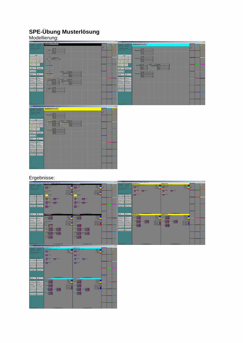
SPE-Übung Musterlösung Modellierung:
Ergebnisse:
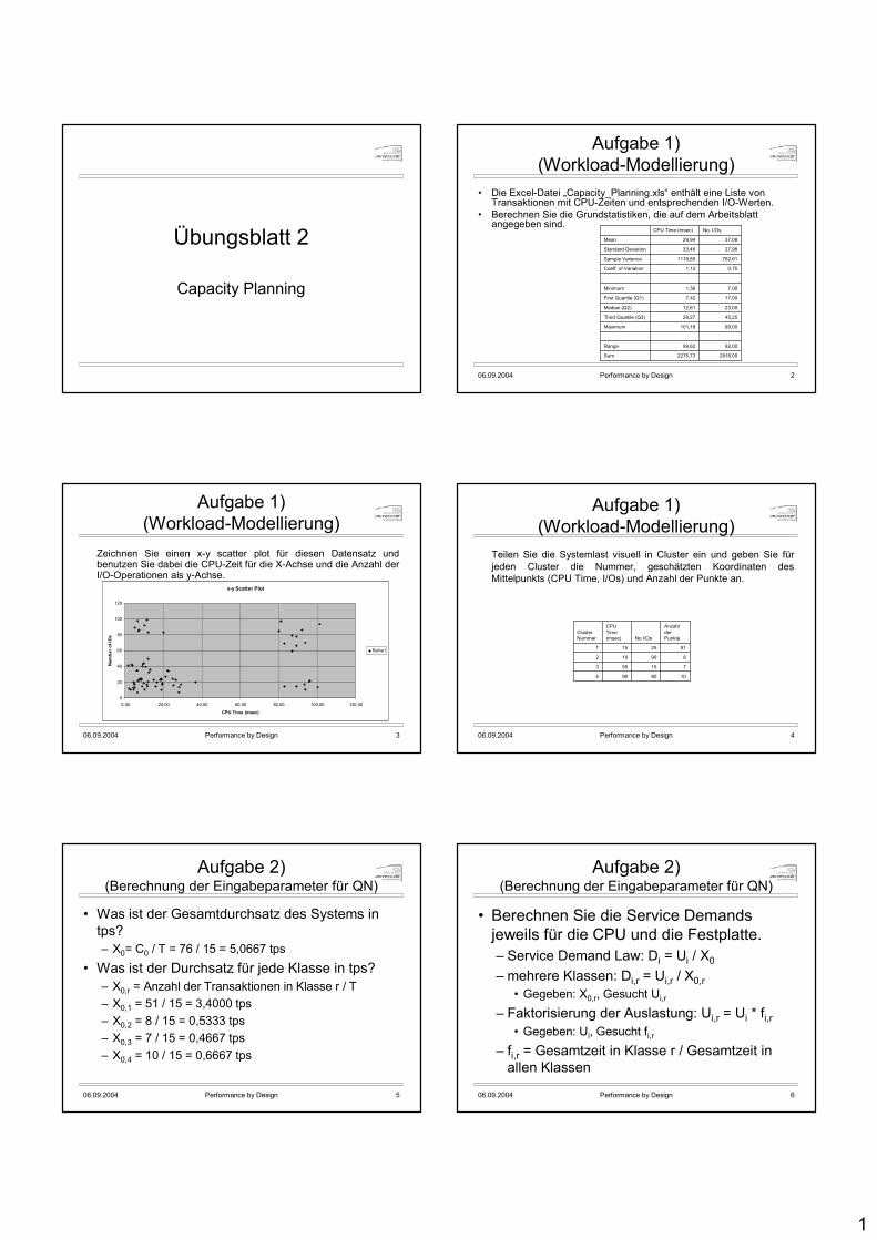
1
Übungsblatt 2
Capacity Planning
06.09.2004 Performance by Design 2
Aufgabe 1) (Workload-Modellierung)
• Die Excel-Datei „Capacity_Planning.xls“ enthält eine Liste von Transaktionen mit CPU-Zeiten und entsprechenden I/O-Werten.
• Berechnen Sie die Grundstatistiken, die auf dem Arbeitsblatt angegeben sind.
2818,002275,73Sum
92,0099,62Range
99,00101,18Maximum
45,2528,27Third Quartile (Q3)
23,0012,61Median (Q2)
17,007,42First Quartile (Q1)
7,001,56Minimum
0,751,12Coeff. of Variation
782,611119,85Sample Variance
27,9833,46Standard Deviation
37,0829,94Mean
No. I/OsCPU Time (msec)
06.09.2004 Performance by Design 3
Aufgabe 1) (Workload-Modellierung)
• Zeichnen Sie einen x-y scatter plot für diesen Datensatz und benutzen Sie dabei die CPU-Zeit für die X-Achse und die Anzahl der I/O-Operationen als y-Achse.
x-y Scatter Plot
0
20
40
60
80
100
120
0,00 20,00 40,00 60,00 80,00 100,00 120,00
CPU Time (msec)
Num
bero
fIO
s
Reihe1
06.09.2004 Performance by Design 4
Aufgabe 1) (Workload-Modellierung)
• Teilen Sie die Systemlast visuell in Cluster ein und geben Sie für jeden Cluster die Nummer, geschätzten Koordinaten des Mittelpunkts (CPU Time, I/Os) und Anzahl der Punkte an.
1080904
715953
890102
5125151
Anzahl der PunkteNo I/Os
CPU Time (msec)
Cluster Nummer
06.09.2004 Performance by Design 5
Aufgabe 2) (Berechnung der Eingabeparameter für QN)
• Was ist der Gesamtdurchsatz des Systems in tps? – X0= C0 / T = 76 / 15 = 5,0667 tps
• Was ist der Durchsatz für jede Klasse in tps? – X0,r = Anzahl der Transaktionen in Klasse r / T– X0,1 = 51 / 15 = 3,4000 tps– X0,2 = 8 / 15 = 0,5333 tps– X0,3 = 7 / 15 = 0,4667 tps– X0,4 = 10 / 15 = 0,6667 tps
06.09.2004 Performance by Design 6
Aufgabe 2) (Berechnung der Eingabeparameter für QN)
• Berechnen Sie die Service Demandsjeweils für die CPU und die Festplatte. – Service Demand Law: Di = Ui / X0
– mehrere Klassen: Di,r = Ui,r / X0,r• Gegeben: X0,r, Gesucht Ui,r
– Faktorisierung der Auslastung: Ui,r = Ui * fi,r• Gegeben: Ui, Gesucht fi,r
– fi,r = Gesamtzeit in Klasse r / Gesamtzeit in allen Klassen
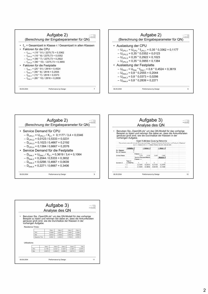
2
06.09.2004 Performance by Design 7
Aufgabe 2) (Berechnung der Eingabeparameter für QN)
• fi,r = Gesamtzeit in Klasse r / Gesamtzeit in allen Klassen• Faktoren für die CPU
– fCPU,1 = (15 * 51) / 2275,73 = 0,3362– fCPU,2 = (10 * 8) / 2275,73 = 0,0352– fCPU,3 = (95 * 7) / 2275,73 = 0,2922– fCPU,4 = (90 * 10) / 2275,73 = 0,3955
• Faktoren für die Festplatte– fDisk,1 = (25 * 51) / 2818 = 0,4524– fDisk,2 = (90 * 8) / 2818 = 0,2555– fDisk,3 = (15 * 7) / 2818 = 0,0373– fDisk,4 = (80 * 10) / 2818 = 0,2839
06.09.2004 Performance by Design 8
Aufgabe 2) (Berechnung der Eingabeparameter für QN)
• Auslastung der CPU– UCPU,1 = UCPU * fCPU,1 = 0,35 * 0,3362 = 0,1177– UCPU,2 = 0,35 * 0,0352 = 0,0123– UCPU,3 = 0,35 * 0,2922 = 0,1023– UCPU,4 = 0,35 * 0,3955 = 0,1384
• Auslastung der Festplatte– UDisk,1 = UDisk * fDisk,1 = 0,8 * 0,4524 = 0,3619– UDisk,2 = 0,8 * 0,2555 = 0,2044– UDisk,3 = 0,8 * 0,0373 = 0,0298– UDisk,4 = 0,8 * 0,2839 = 0,2271
06.09.2004 Performance by Design 9
Aufgabe 2) (Berechnung der Eingabeparameter für QN)
• Service Demand für CPU– DCPU,1 = UCPU,1 / X0,1 = 0,1177 / 3,4 = 0,0346– DCPU,2 = 0,0123 / 0,5333 = 0,0231– DCPU,3 = 0,1023 / 0,4667 = 0,2192– DCPU,4 = 0,1384 / 0,6667 = 0,2076
• Service Demand für die Festplatte– DDisk,1 = UDisk,1 / X0,1 = 0,3619 / 3,4 = 0,1064– DDisk,2 = 0,2044 / 0,5333 = 0,3832– DDisk,3 = 0,0298 / 0,4667 = 0,0639– DDisk,4 = 0,2271 / 0,6667 = 0,3406
06.09.2004 Performance by Design 10
Aufgabe 3)Analyse des QN
• Benutzen Sie „OpenQN.xls“ um das QN-Modell für das vorherige Beispiel zu lösen und nehmen Sie dabei an, dass die Ankunftsraten genauso groß sind, wie die Durchsätze der Klassen in der vorherigen Aufgabe.
06.09.2004 Performance by Design 11
Aufgabe 3)Analyse des QN
• Benutzen Sie „OpenQN.xls“ um das QN-Modell für das vorherige Beispiel zu lösen und nehmen Sie dabei an, dass die Ankunftsraten genauso groß sind, wie die Durchsätze der Klassen in der vorherigen Aufgabe.
2,254520,709442,202020,65621Response Time
1,924590,361072,165300,60122Disk
0,329940,348370,036710,05499CPU
Class 4Class 3Class 2Class 1
Residence Times:
0,823030,227180,029840,204250,36176Disk
0,370790,138470,102370,012310,11764CPU
TotalClass 4Class 3Class 2Class 1
Utilizations:

umlPSI Musterlösung

l
E. Tasks of the experiment
The task for the experiment contains design-documents for the investigated prototypical webser-ver. It was tried to arrange the inputs as equal as possible for all approaches, but e. g. theUML-diagramms are not contained into the task for Capacity Planning, as it would be uselessfor it. Further details are available in section 3.2.
Remark: For this translation the task for SPE is translated exemplarily. The following textrefers to original tasks beginning with the side ”Studie Performance-Evaluationstechniken –Software Performance Engineering“.
E.1. Task
[”Studie Performance-Evaluationstechniken“ – Software Performance Engineering – Task, trans-lation from the original documents below]
A novel componentbased webserver shall be developed. During the design the developersdiscuss the different alternatives for the architecture. As they are familiar with performance-analysis, they are adviced to evaluated the performance-properties of each design-alternative.
The developers present a component- and sequence-diagram for the design-alternative. Asystem-administrator delivers the data about hardware for the webserver. Your task is to usethe skilled approach of Software Performance Engineering (SPE) to determine the performance-values of the given design-alternatives. Afterwards you should give a recommendation, whichdesign-alternative would probably be the best from the performance-oriented point of view.Your tasks are:
• Create, according to the sequence-diagramm, the neccessary execution-graph using thetool SPE-ED.
• Choose the menu ”overhead/specify overhes“, select in the dialog ”select spec template“the button ”new“ and in the dialog ”select facility template“ the button ”show all“. Choosefrom the list the facility template ”NachtF Server“. Put the data (see below: ProcessingOverhead) to the shown table.
• Determine for each node from the execution-graph the ”Software Resource Requirements“.If no default values are given, try to estimate the values, try to estimate realistically.
• Calculate the Residence Times, Resource Usages and Utilizations for all design-alternativesand put your results in the foreseen table. Note advantages and disadvantages for eachalternative.
• Favourize one of the modeled design-decisions and give reasons for your decision. Do notonly orient to the calculated performance-values, take all available factors into account.
li

E. Tasks of the experiment
E.2. Component-diagram
[see below: original document]
E.3. Sequence-diagram
[see below: original document]
E.4. Further settings
• The ”HTTP“-calls in the sequence-diagramm model HTTP-get requests, which come fromthe client respectively the answer from the server. The connection uses the internet.
• For statical HTML-pages the webserver accesses (probability 40%) its local harddisk.
• Requests for dynamic HTML-pages (probalility 60%) get their data from external appli-cations (by a local area network), which are executed on a different server. The externalapplication takes averaged 0.5 seconds to collect the required data.
• There is no delay for user input in this modell. Only the performance of single requests,not a full sequence is measuresd. The delay given in the process overhead should be usedas calculating-time for the external application.
• Average size of send files: about 5 KByte.
• The arrival rate of new request will be about 1 per second.
• The webserver is multithreaded and starts in the component ”DispatcherThread“ a newthread for each request.
E.5. Software Resources
• Workload: the time for calculation on the CPU (Example: value ”5“ means, that thecalculation takes 500 microsecond on the CPU)
• DiskAccess: the number of harddisk-accesses
• INetMsgSize: the size of a request (in KByte), that is send over the internet
• LANMsgSize: the size of a request, that is send over LAN in KByte
• ExtApp: the time of calculation for the external application in seconds
lii

E.6. Processing Overhead
E.6. Processing Overhead
[See the table for values.]The service times have been determined as follows:
• CPU: by measuring
• Disk: specification: 3 ms per I/O
• INet: 64 KBit/sec (ISDN) → 8 KB/sec → 0,125 sec/KB
• LAN: 10 MBit/sec (Ethernet) → 1250 KB/sec → 0,0008 sec/KB
• Delay: arbitrary setting, might be changed
E.7. Resourcedistribution (just for illustration)
[”Ressourcenverteilung (nur zur Illustration)“]
E.8. Design-alternatives
[”Entwurfsalternativen“ – For each alternative the sequence-diagramm, the componente-diagrammand a description are given. The alternatives are described in chapter 3.2.3.]
liii
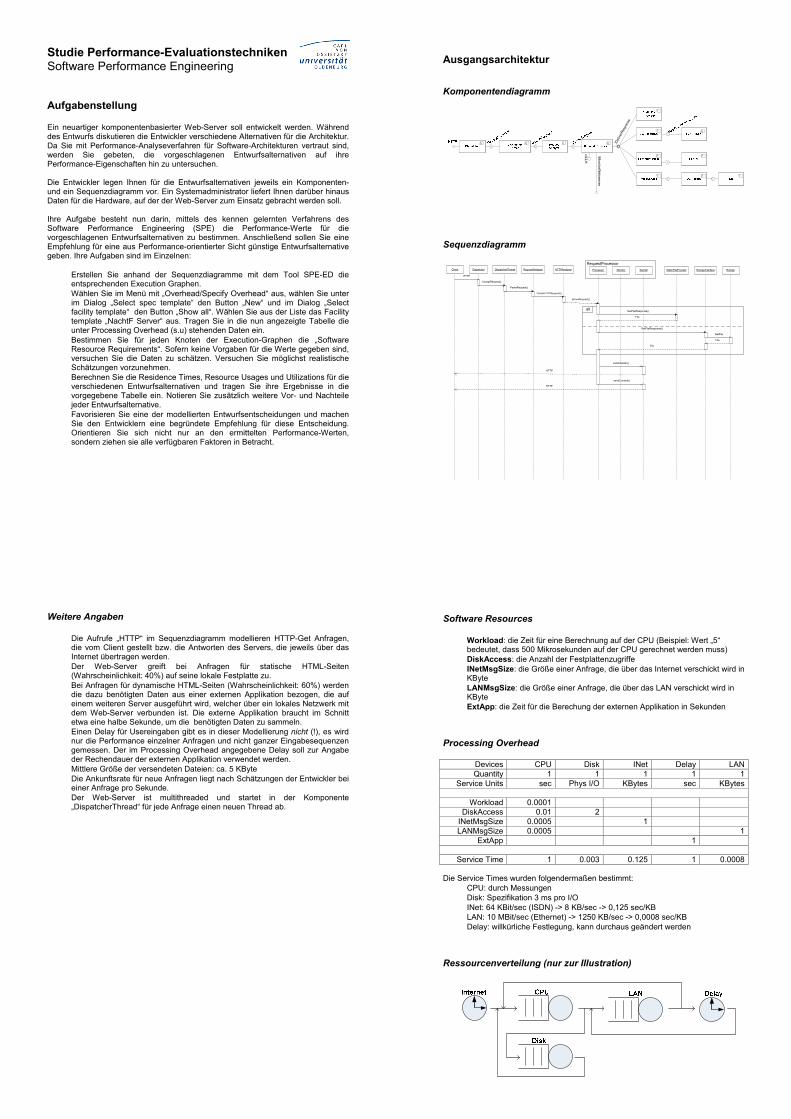
Studie Performance-Evaluationstechniken Software Performance Engineering
Aufgabenstellung Ein neuartiger komponentenbasierter Web-Server soll entwickelt werden. Während des Entwurfs diskutieren die Entwickler verschiedene Alternativen für die Architektur. Da Sie mit Performance-Analyseverfahren für Software-Architekturen vertraut sind, werden Sie gebeten, die vorgeschlagenen Entwurfsalternativen auf ihre Performance-Eigenschaften hin zu untersuchen. Die Entwickler legen Ihnen für die Entwurfsalternativen jeweils ein Komponenten- und ein Sequenzdiagramm vor. Ein Systemadministrator liefert Ihnen darüber hinaus Daten für die Hardware, auf der der Web-Server zum Einsatz gebracht werden soll. Ihre Aufgabe besteht nun darin, mittels des kennen gelernten Verfahrens des Software Performance Engineering (SPE) die Performance-Werte für die vorgeschlagenen Entwurfsalternativen zu bestimmen. Anschließend sollen Sie eine Empfehlung für eine aus Performance-orientierter Sicht günstige Entwurfsalternative geben. Ihre Aufgaben sind im Einzelnen:
• Erstellen Sie anhand der Sequenzdiagramme mit dem Tool SPE-ED die entsprechenden Execution Graphen.
• Wählen Sie im Menü mit „Overhead/Specify Overhead“ aus, wählen Sie unter im Dialog „Select spec template“ den Button „New“ und im Dialog „Select facility template“ den Button „Show all“. Wählen Sie aus der Liste das Facility template „NachtF Server“ aus. Tragen Sie in die nun angezeigte Tabelle die unter Processing Overhead (s.u) stehenden Daten ein.
• Bestimmen Sie für jeden Knoten der Execution-Graphen die „Software Resource Requirements“. Sofern keine Vorgaben für die Werte gegeben sind, versuchen Sie die Daten zu schätzen. Versuchen Sie möglichst realistische Schätzungen vorzunehmen.
• Berechnen Sie die Residence Times, Resource Usages und Utilizations für die verschiedenen Entwurfsalternativen und tragen Sie ihre Ergebnisse in die vorgegebene Tabelle ein. Notieren Sie zusätzlich weitere Vor- und Nachteile jeder Entwurfsalternative.
• Favorisieren Sie eine der modellierten Entwurfsentscheidungen und machen Sie den Entwicklern eine begründete Empfehlung für diese Entscheidung. Orientieren Sie sich nicht nur an den ermittelten Performance-Werten, sondern ziehen sie alle verfügbaren Faktoren in Betracht.
Ausgangsarchitektur
Komponentendiagramm
HTT
P IMonitorW
ebserver
IDeli
verR
espo
nse
Sequenzdiagramm
alt
Client Dispatcher DispatcherThread RequestAnalyzer Processor StaticFileProviderHTTPAnalyser Monitor Sender
RequestProcessor
File
HTTP
HTTP
sendHeader()
sendContent()
HTTP
ParseHTTPRequest()
ServeRequest()
ParseRequest()
AcceptRequest()
ExtAppInterface ExtApp
GetFile
File
File
GetFileResponse()
GetFileResponse()
Weitere Angaben
• Die Aufrufe „HTTP“ im Sequenzdiagramm modellieren HTTP-Get Anfragen, die vom Client gestellt bzw. die Antworten des Servers, die jeweils über das Internet übertragen werden.
• Der Web-Server greift bei Anfragen für statische HTML-Seiten (Wahrscheinlichkeit: 40%) auf seine lokale Festplatte zu.
• Bei Anfragen für dynamische HTML-Seiten (Wahrscheinlichkeit: 60%) werden die dazu benötigten Daten aus einer externen Applikation bezogen, die auf einem weiteren Server ausgeführt wird, welcher über ein lokales Netzwerk mit dem Web-Server verbunden ist. Die externe Applikation braucht im Schnitt etwa eine halbe Sekunde, um die benötigten Daten zu sammeln.
• Einen Delay für Usereingaben gibt es in dieser Modellierung nicht (!), es wird nur die Performance einzelner Anfragen und nicht ganzer Eingabesequenzen gemessen. Der im Processing Overhead angegebene Delay soll zur Angabe der Rechendauer der externen Applikation verwendet werden.
• Mittlere Größe der versendeten Dateien: ca. 5 KByte • Die Ankunftsrate für neue Anfragen liegt nach Schätzungen der Entwickler bei
einer Anfrage pro Sekunde. • Der Web-Server ist multithreaded und startet in der Komponente
„DispatcherThread“ für jede Anfrage einen neuen Thread ab.
Software Resources
• Workload: die Zeit für eine Berechnung auf der CPU (Beispiel: Wert „5“ bedeutet, dass 500 Mikrosekunden auf der CPU gerechnet werden muss)
• DiskAccess: die Anzahl der Festplattenzugriffe • INetMsgSize: die Größe einer Anfrage, die über das Internet verschickt wird in
KByte • LANMsgSize: die Größe einer Anfrage, die über das LAN verschickt wird in
KByte • ExtApp: die Zeit für die Berechung der externen Applikation in Sekunden
Processing Overhead
Devices CPU Disk INet Delay LANQuantity 1 1 1 1 1
Service Units sec Phys I/O KBytes sec KBytes
Workload 0.0001DiskAccess 0.01 2
INetMsgSize 0.0005 1LANMsgSize 0.0005 1
ExtApp 1
Service Time 1 0.003 0.125 1 0.0008
Die Service Times wurden folgendermaßen bestimmt: • CPU: durch Messungen • Disk: Spezifikation 3 ms pro I/O • INet: 64 KBit/sec (ISDN) -> 8 KB/sec -> 0,125 sec/KB • LAN: 10 MBit/sec (Ethernet) -> 1250 KB/sec -> 0,0008 sec/KB • Delay: willkürliche Festlegung, kann durchaus geändert werden
Ressourcenverteilung (nur zur Illustration)
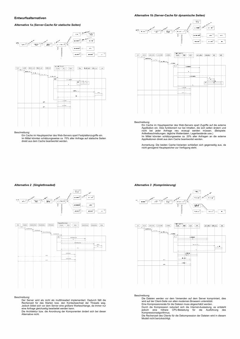
Entwurfsalternativen Alternative 1a (Server-Cache für statische Seiten)
HTT
P IMonitorW
ebserver
IDel
iverR
espo
nse
Beschreibung: • Ein Cache im Hauptspeicher des Web-Servers spart Festplattenzugriffe ein. • Im Mittel könnten schätzungsweise ca. 70% aller Anfrage auf statische Seiten
direkt aus dem Cache beantwortet werden.
Alternative 1b (Server-Cache für dynamische Seiten)
HTT
P IMonitorW
ebserver
IDeli
verR
espo
nse
Beschreibung: • Ein Cache im Hauptspeicher des Web-Servers spart Zugriffe auf die externe
Applikation ein. Dies funktioniert nur bei Inhalten, die sich selten ändern und nicht bei jeder Anfrage neu erzeugt werden müssen. (Beispiele: Artikelbeschreibungen, tägliche Wetterdaten, Lagerbestände usw.)
• Im Mittel könnten schätzungsweise ca. 20% aller Anfragen an die externe Applikationen direkt aus dem Cache beantwortet werden.
• Anmerkung: Die beiden Cache-Varianten schließen sich gegenseitig aus, da
nicht genügend Hauptspeicher zur Verfügung steht.
Alternative 2 (Singlethreaded)
HTT
P IMonitorW
ebserver
IDeli
verR
espo
nse
alt
Client Dispatcher DispatcherThread RequestAnalyzer Processor StaticFileProviderHTTPAnalyser Monitor Sender
RequestProcessor
File
HTTP
HTTP
sendHeader()
sendContent()
HTTP
ParseHTTPRequest()
ServeRequest()
ParseRequest()
AcceptRequest()
ExtAppInterface ExtApp
GetFile
File
File
GetFileResponse()
GetFileResponse()
Beschreibung: • Der Server wird als nicht als multihreaded implementiert. Dadurch fällt die
Rechenzeit für das Starten bzw. den Kontextwechsel der Threads weg. Jedoch bildet sich vor dem Server eine größere Warteschlange, da immer nur eine Anfrage gleichzeitig bearbeitet werden kann.
• Die Architektur bzw. die Anordnung der Komponenten ändert sich bei dieser Alternative nicht.
Alternative 3 (Komprimierung)
HTT
P IMonitorW
ebserver
IDeli
verR
espo
nse
IGetDatabaseContent
Beschreibung: • Die Dateien werden vor dem Versenden auf dem Server komprimiert, dies
wird auf der Client-Seite von allen modernen Browsern unterstützt. • Eine Kompressionsrate für die Dateien muss abgeschätzt werden. • Durch die Kompression reduziert sich die Internet-Auslastung, es entsteht
jedoch eine höhere CPU-Belastung für die Ausführung des Kompressionsalgorithmus.
• Die Rechenzeit des Clients für die Dekompression der Dateien wird in diesem Modell nicht berücksichtigt.
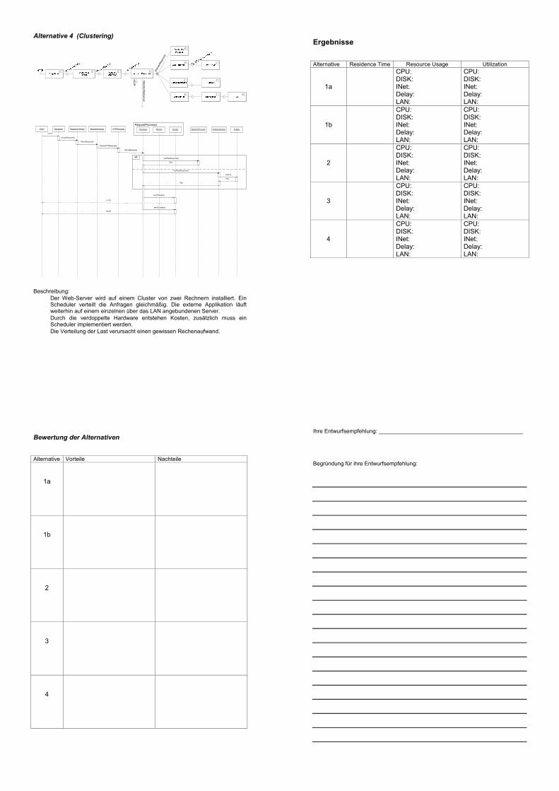
Alternative 4 (Clustering)
HTT
P IMonitorW
ebserver
IDeli
verR
espo
nse
alt
Client Dispatcher DispatcherThread RequestAnalyzer Processor StaticFileProviderHTTPAnalyser Monitor Sender
RequestProcessor
File
HTTP
HTTP
sendHeader()
sendContent()
HTTP
ParseHTTPRequest()
ServeRequest()
ParseRequest()
AcceptRequest()
ExtAppInterface ExtApp
GetFile
File
File
GetFileResponse()
GetFileResponse()
Beschreibung: • Der Web-Server wird auf einem Cluster von zwei Rechnern installiert. Ein
Scheduler verteilt die Anfragen gleichmäßig. Die externe Applikation läuft weiterhin auf einem einzelnen über das LAN angebundenen Server.
• Durch die verdoppelte Hardware entstehen Kosten, zusätzlich muss ein Scheduler implementiert werden.
• Die Verteilung der Last verursacht einen gewissen Rechenaufwand.
Ergebnisse
Alternative Residence Time Resource Usage Utilization
1a
CPU: DISK: INet: Delay: LAN:
CPU: DISK: INet: Delay: LAN:
1b
CPU: DISK: INet: Delay: LAN:
CPU: DISK: INet: Delay: LAN:
2
CPU: DISK: INet: Delay: LAN:
CPU: DISK: INet: Delay: LAN:
3
CPU: DISK: INet: Delay: LAN:
CPU: DISK: INet: Delay: LAN:
4
CPU: DISK: INet: Delay: LAN:
CPU: DISK: INet: Delay: LAN:
Bewertung der Alternativen
Alternative Vorteile Nachteile
1a
1b
2
3
4
Ihre Entwurfsempfehlung: ______________________________________________
Begründung für ihre Entwurfsempfehlung:
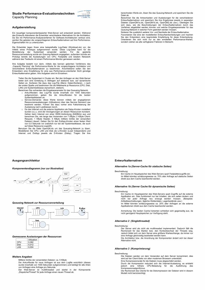
Studie Performance-Evaluationstechniken Capacity Planning
Aufgabenstellung Ein neuartiger komponentenbasierter Web-Server soll entwickelt werden. Während des Entwurfs diskutieren die Entwickler verschiedene Alternativen für die Architektur. Da Sie mit Performance-Analyseverfahren für Software-Architekturen vertraut sind, werden Sie gebeten die vorgeschlagenen Entwurfsalternativen auf ihre Performance-Eigenschaften hin zu untersuchen. Die Entwickler legen Ihnen eine beispielhafte Log-Datei (Workload.xls) vor, die mittels eines Prototyps aufgenommen wurde. Diese Log-Datei kann für die Modellierung der Systemlast verwendet werden. Für die geplante Ressourcenverteilung wurde ein Queuing-Network angegeben, außerdem konnte am Prototyp bereits die Auslastungen von CPU, Festplatte und lokalem Netzwerk während des Testlaufs mit einem Performance-Monitor gemessen werden. Ihre Aufgabe besteht nun darin, mittels des kennen gelernten Verfahrens des „Capacity Planning“ die Performance-Werte für die vorgeschlagene Architektur und verschiedene Entwurfsalternativen zu bestimmen. Anschließend sollen Sie den Entwicklern eine Empfehlung für eine aus Performance-orientierter Sicht günstige Entwurfsalternative geben. Ihre Aufgaben sind im Einzelnen:
• Teilen Sie die Systemlast in Cluster ein. Bei den Anfragen an den Web-Server bietet sich eine Einteilung in Abfragen auf statische bzw. auf dynamische Seiten an. Sortieren Sie dazu das Log-File (Menü: Daten/Sortieren…) nach der ersten Spalte und bestimmen Sie die Mittelwerte je Ressource (CPU, Disk, LAN) und Systemlastklasse (dynamisch, statisch).
• Berechnen Sie vorhanden die Eingabeparameter für das Queueing Network. o Ankunftsraten: das Log-File wurde innerhalb von 1000 Sekunden
aufgenommen, geben Sie die Ankunftsraten für die beiden Systemlastklassen an.
o Service-Demands: diese Werte können mittels der angegebenen Ressourcenauslastungen (Utilizations) über das Service Demand Law bestimmt werden. Führen Sie dazu vorher eine Faktorisierung der Auslastung nach Lastklassen durch.
o Da das Internet und die externe Applikation als Delay-Knoten modelliert wurden (s.u.), sind die Verzögerungen an diesen Ressourcen konstant. Gehen beim Internet von einer ISDN-Verbindung (64KBit/s) aus und berechnen Sie, wie lange das Versenden von 7 KByte (1 KByte Client-Request, 1 KByte Header, 5 KByte mittlere Größe der versandten Dateien) dauert. Geben Sie für den ExtApp-Knoten einen festen Wert von 0,5 Sekunde vor (natürlich nur bei der Systemlastklasse, die auch auf diese Ressource zugreift).
• Benutzen Sie die Datei OpenQN.xls um das Queueing-Network zu lösen. Modellieren Sie CPU, LAN und Disk als LI-Knoten (Load Independent) und Internet und ExtApp jeweils als D-Knoten (Delay). Tragen Sie ihre
berechneten Werte ein, lösen Sie das Queuing-Network und speichern Sie die Datei ab.
• Berechnen Sie die Antwortzeiten und Auslastungen für die verschiedenen Entwurfsalternativen und speichern Sie ihre Ergebnisse jeweils in separaten Dateien (OpenQN1a.xls, OpenQN1b.xls, OpenQN2.xls usw.). Überlegen Sie sich dazu, wie die Beschreibungen der Entwurfsalternativen durch das Verfahren abgebildet werden können und welche Eingabeparameter für das Queuing-Network in welcher Form geändert werden müssen.
• Notieren Sie zusätzlich weitere Vor- und Nachteile der Entwurfsalternative. • Favorisieren Sie eine der modellierten Entwurfsentscheidungen und machen
Sie den Entwicklern eine begründete Empfehlung für diese Entscheidung. Orientieren Sie sich nicht nur an den ermittelten Performance-Werten, sondern ziehen sie alle verfügbaren Faktoren in Betracht.
Ausgangsarchitektur
Komponentendiagramm (nur zur Illustration)
HTT
P IMonitorW
ebserver
IDeli
verR
espo
nse
Queueing Network zur Ressourcenverteilung
Gemessene Auslastungen der Ressourcen Utilization CPU 0,082 Disk 0,012 LAN 0,004
Weitere Angaben • Mittlere Größe der versendeten Dateien: ca. 5 KByte • Die Ankunftsrate für neue Anfragen ist aus dem Logfile ersichtlich (dieses
wurde innerhalb von 1000 Sekunden aufgenommen) und beträgt für alle Arten von Anfragen eine Anfrage pro Sekunde.
• Der Web-Server ist multithreaded und startet in der Komponente „DispatcherThread“ für jede Anfrage einen neuen Thread ab.
Entwurfsalternativen Alternative 1a (Server-Cache für statische Seiten) Beschreibung:
• Ein Cache im Hauptspeicher des Web-Servers spart Festplattenzugriffe ein. • Im Mittel könnten schätzungsweise ca. 70% aller Anfrage auf statische Seiten
direkt aus dem Cache beantwortet werden.
Alternative 1b (Server Cache für dynamische Seiten) Beschreibung:
• Ein Cache im Hauptspeicher des Web-Servers spart Zugriffe auf die externe Applikation ein. Dies funktioniert nur bei Inhalten, die sich selten ändern und nicht bei jeder Anfrage neu erzeugt werden müssen. (Beispiele: Artikelbeschreibungen, tägliche Wetterdaten, Lagerbestände usw.)
• Im Mittel könnten schätzungsweise ca. 20% aller Anfragen an die externe Applikationen direkt aus dem Cache beantwortet werden.
• Anmerkung: Die beiden Cache-Varianten schließen sich gegenseitig aus, da
nicht genügend Hauptspeicher zur Verfügung steht.
Alternative 2 (Singlethreaded) Beschreibung:
• Der Server wird als nicht als multihreaded implementiert. Dadurch fällt die Rechenzeit für das Starten bzw. den Kontextwechsel der Threads weg. Jedoch bildet sich vor dem Server eine größere Warteschlange, da immer nur eine Anfrage gleichzeitig bearbeitet werden kann.
• Die Architektur bzw. die Anordnung der Komponenten ändert sich bei dieser Alternative nicht.
Alternative 3 (Komprimierung) Beschreibung:
• Die Dateien werden vor dem Versenden auf dem Server komprimiert, dies wird auf der Client-Seite von allen modernen Browsern unterstützt.
• Eine Kompressionsrate für die Dateien muss abgeschätzt werden. • Durch die Kompression reduziert sich die Internet-Auslastung, es entsteht
jedoch eine höhere CPU-Belastung für die Ausführung des Kompressionsalgorithmus.
• Die Rechenzeit des Clients für die Dekompression der Dateien wird in diesem Modell nicht berücksichtigt.
Alternative 4 (Clustering) Beschreibung:
• Der Web-Server wird auf einem Cluster von zwei Rechnern installiert. Ein Scheduler verteilt die Anfragen gleichmäßig. Die externe Applikation läuft weiterhin auf einem einzelnen über das LAN angebundenen Server.
• Durch die verdoppelte Hardware entstehen Kosten, zusätzlich muss ein Scheduler implementiert werden.
• Die Verteilung der Last verursacht einen gewissen Rechenaufwand. • Hinweis: die LI-Knoten im QN für CPU und Disk können in MP2-Knoten
umgewandelt werden
Ergebnisse Alternative Vorteile Nachteile
1a
1b
2
3
4
Bewertung der Alternativen
Ihre Entwurfsempfehlung: ______________________________________________
Begründung für ihre Entwurfsempfehlung:
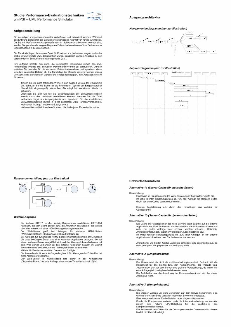
Studie Performance-Evaluationstechniken umlPSI – UML Performance Simulator
Aufgabenstellung Ein neuartiger komponentenbasierter Web-Server soll entwickelt werden. Während des Entwurfs diskutieren die Entwickler verschiedene Alternativen für die Architektur. Da Sie mit Performance-Analyseverfahren für Software-Architekturen vertraut sind, werden Sie gebeten die vorgeschlagenen Entwurfsalternativen auf ihre Performance-Eigenschaften hin zu untersuchen. Die Entwickler legen Ihnen eine Datei für Poseidon vor (webserver.zargo), in der der grobe Entwurf mittels UML dokumentiert wurde. Zusätzlich wurden Angaben zu den verschiedenen Entwurfsalternativen gemacht (s.u.). Ihre Aufgabe besteht nun darin, die vorgelegten Diagramme mittels des UML Performance Profiles mit sinnvollen Performance-Werten zu attributieren. Danach erstellen Sie Modelle für die einzelnen Entwurfsalternativen und speichern diese jeweils in separaten Dateien ab. Die Simulation der Modelle kann im Rahmen dieses Versuchs nicht durchgeführt werden und erfolgt nachträglich. Ihre Aufgaben sind im Einzelnen:
• Tragen Sie die noch fehlenden Werte in den Tagged-Values der Diagramme ein. Schätzen Sie die Dauer für die PAdemand-Tags (in der Eingabedatei ist überall 0.0 eingetragen!). Versuchen Sie möglichst realistische Werte zu schätzen.
• Überlegen Sie sich wie Sie die Beschreibungen der Entwurfsalternativen jeweils durch das Verfahren modellieren können. Nehmen Sie die Datei ‚webserver.zargo’ als Ausgangsbasis und speichern Sie die modellierten Entwurfsalternativen jeweils in einer separaten Datei (‚webserver1a.zargo’, ‚webserver1b.zargo’, webserver2.zargo usw.).
• Notieren Sie zusätzlich weitere Vor- und Nachteile jeder Entwurfsalternative.
Ausgangsarchitektur
Komponentendiagramm (nur zur Illustration)
HTT
P IMonitorW
ebserver
IDeli
verR
espo
nse
IGetDatabaseContent
Sequenzdiagramm (nur zur Illustration)
Ressourcenverteilung (nur zur Illustration)
Weitere Angaben
• Die Aufrufe „HTTP“ in den Activity-Diagrammen modellieren HTTP-Get Anfragen, die vom Client gestellt bzw. die Antworten des Servers, die jeweils über das Internet mit einer ISDN-Leitung übertragen werden.
• Der Web-Server greift bei Anfragen für statische HTML-Seiten (Wahrscheinlichkeit: 40%) auf seine lokale Festplatte zu.
• Bei Anfragen für dynamische HTML-Seiten (Wahrscheinlichkeit: 60%) werden die dazu benötigten Daten aus einer externen Applikation bezogen, die auf einem weiteren Server ausgeführt wird, welcher über ein lokales Netzwerk mit dem Web-Server verbunden ist. Die externe Applikation braucht im Schnitt etwa eine halbe Sekunde, um die benötigten Daten zu sammeln.
• Mittlere Größe der versendeten Dateien: ca. 5 KByte • Die Ankunftsrate für neue Anfragen liegt nach Schätzungen der Entwickler bei
einer Anfrage pro Sekunde. • Der Web-Server ist multithreaded und startet in der Komponente
„DispatcherThread“ für jede Anfrage einen neuen Thread (maximal 10) ab.
Entwurfsalternativen Alternative 1a (Server-Cache für statische Seiten) Beschreibung:
• Ein Cache im Hauptspeicher des Web-Servers spart Festplattenzugriffe ein. • Im Mittel könnten schätzungsweise ca. 70% aller Anfrage auf statische Seiten
direkt aus dem Cache beantwortet werden.
• Hinweis: Modellierung z.B. durch das Hinzufügen eine Aktivität für Cachezugriffe
Alternative 1b (Server-Cache für dynamische Seiten) Beschreibung:
• Ein Cache im Hauptspeicher des Web-Servers spart Zugriffe auf die externe Applikation ein. Dies funktioniert nur bei Inhalten, die sich selten ändern und nicht bei jeder Anfrage neu erzeugt werden müssen. (Beispiele: Artikelbeschreibungen, tägliche Wetterdaten, Lagerbestände usw.)
• Im Mittel könnten schätzungsweise ca. 20% aller Anfragen an die externe Applikationen direkt aus dem Cache beantwortet werden.
• Anmerkung: Die beiden Cache-Varianten schließen sich gegenseitig aus, da
nicht genügend Hauptspeicher zur Verfügung steht.
Alternative 2 (Singlethreaded) Beschreibung:
• Der Server wird als nicht als multihreaded implementiert. Dadurch fällt die Rechenzeit für das Starten bzw. den Kontextwechsel der Threads weg. Jedoch bildet sich vor dem Server eine größere Warteschlange, da immer nur eine Anfrage gleichzeitig bearbeitet werden kann.
• Die Architektur bzw. die Anordnung der Komponenten ändert sich bei dieser Alternative nicht.
Alternative 3 (Komprimierung) Beschreibung:
• Die Dateien werden vor dem Versenden auf dem Server komprimiert, dies wird auf der Client-Seite von allen modernen Browsern unterstützt.
• Eine Kompressionsrate für die Dateien muss abgeschätzt werden. • Durch die Kompression reduziert sich die Internet-Auslastung, es entsteht
jedoch eine höhere CPU-Belastung für die Ausführung des Kompressionsalgorithmus.
• Die Rechenzeit des Clients für die Dekompression der Dateien wird in diesem Modell nicht berücksichtigt.

Alternative 4 (Clustering)
Beschreibung: • Der Web-Server wird auf einem Cluster von zwei Rechnern installiert. Ein
Scheduler verteilt die Anfragen gleichmäßig. Die externe Applikation läuft weiterhin auf einem einzelnen über das LAN angebundenen Server.
• Durch die verdoppelte Hardware entstehen Kosten, zusätzlich muss ein Scheduler implementiert werden.
• Die Verteilung der Last verursacht einen gewissen Rechenaufwand.
• Hinweis: Modellierung der verdoppelten Hardware z.B. durch das PArate-Tag in den NodeInstances im Deployment-Diagramm, zusätzlich sollte der Scheduler möglichst einfach modelliert werden (zusätzliche Activity)
Ergebnisse
Alternative
Antwortzeiten
Auslastung
1a
Static: Dynamic:
CPU: Disk: Internet: ExtNode: LAN:
1b
Static: Dynamic:
CPU: Disk: Internet: ExtNode: LAN:
2
Static: Dynamic:
CPU: Disk: Internet: ExtNode: LAN:
3
Static: Dynamic:
CPU: Disk: Internet: ExtNode: LAN:
4
Static: Dynamic:
CPU: Disk: Internet: ExtNode: LAN:
Alternative Vorteile Nachteile
1a
1b
2
3
4
Bewertung der Alternativen
Ihre Entwurfsempfehlung: ______________________________________________
Begründung für ihre Entwurfsempfehlung:
F. Losung des Experiments
Im Folgenden findet sich fur jedes Verfahren eine mogliche Losung der Aufgabenstellung des Ex-periments. Leicht abweichende Modellierungen konnen ebenfalls gultig sein, denn es fließen z.T.individuelle Schatzungen des Entwicklers ein. Die Losung wurde vor dem Experiment erstellt,um die Durchfuhrbarkeit der Aufgabenstellung zu testen. Enthalten sind hier die Ausfuhrungs-graphen des SPE-ED-Werkzeugs jeweils mit Durchlaufzeiten, die Berechnungen fur das CP-Verfahren und die UML-Diagramme, die in Poseidon verwendet wurden.
lxi

SPE - Lösung Alternative 0 Alternative 1a Alternative 1b
Alternative 3 Alternative 4
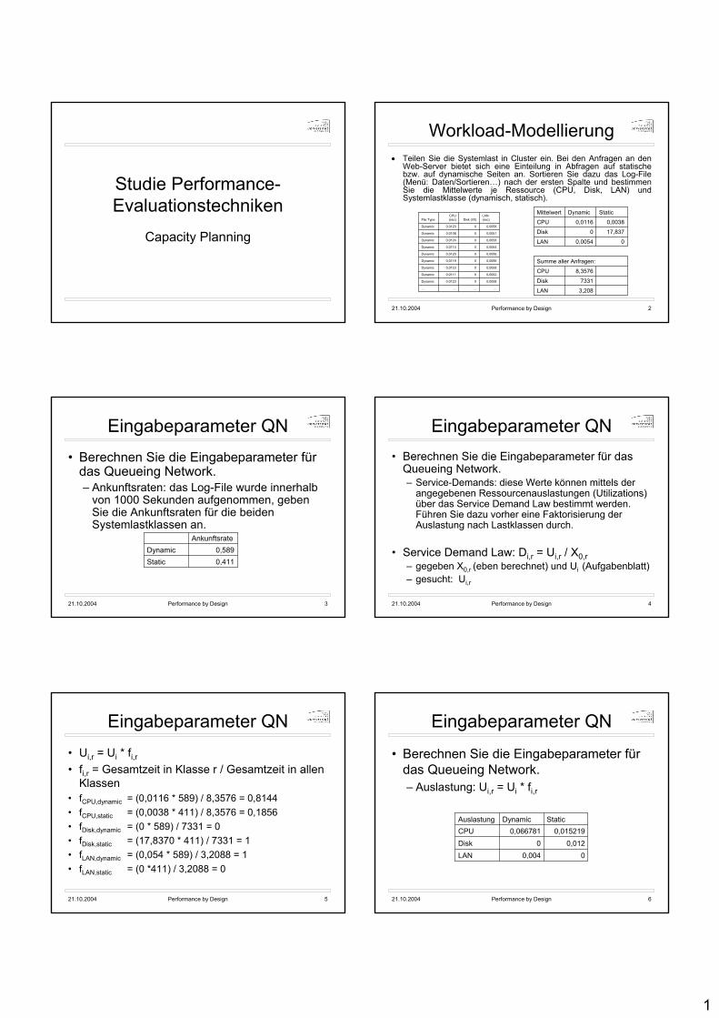
1
Studie Performance-Evaluationstechniken
Capacity Planning
21.10.2004 Performance by Design 2
Workload-Modellierung• Teilen Sie die Systemlast in Cluster ein. Bei den Anfragen an den
Web-Server bietet sich eine Einteilung in Abfragen auf statische bzw. auf dynamische Seiten an. Sortieren Sie dazu das Log-File (Menü: Daten/Sortieren…) nach der ersten Spalte und bestimmen Sie die Mittelwerte je Ressource (CPU, Disk, LAN) und Systemlastklasse (dynamisch, statisch).
7331Disk
00,0054LAN
Summe aller Anfragen:
8,3576CPU
3,208LAN
17,8370Disk
0,00380,0116CPU
StaticDynamicMittelwert
…………
0,005800,0123Dynamic
0,005200,0111Dynamic
0,005800,0123Dynamic
0,005600,0119Dynamic
0,005600,0120Dynamic
0,005400,0114Dynamic
0,005800,0124Dynamic
0,005100,0108Dynamic
0,005800,0123Dynamic
LAN (sec)Disk (I/0)
CPU (sec)File Type
21.10.2004 Performance by Design 3
Eingabeparameter QN• Berechnen Sie die Eingabeparameter für
das Queueing Network.– Ankunftsraten: das Log-File wurde innerhalb
von 1000 Sekunden aufgenommen, geben Sie die Ankunftsraten für die beiden Systemlastklassen an.
0,411Static0,589Dynamic
Ankunftsrate
21.10.2004 Performance by Design 4
Eingabeparameter QN• Berechnen Sie die Eingabeparameter für das
Queueing Network.– Service-Demands: diese Werte können mittels der
angegebenen Ressourcenauslastungen (Utilizations) über das Service Demand Law bestimmt werden. Führen Sie dazu vorher eine Faktorisierung der Auslastung nach Lastklassen durch.
• Service Demand Law: Di,r = Ui,r / X0,r– gegeben X0,r (eben berechnet) und Ui (Aufgabenblatt)– gesucht: Ui,r
21.10.2004 Performance by Design 5
Eingabeparameter QN• Ui,r = Ui * fi,r• fi,r = Gesamtzeit in Klasse r / Gesamtzeit in allen
Klassen• fCPU,dynamic = (0,0116 * 589) / 8,3576 = 0,8144• fCPU,static = (0,0038 * 411) / 8,3576 = 0,1856• fDisk,dynamic = (0 * 589) / 7331 = 0• fDisk,static = (17,8370 * 411) / 7331 = 1• fLAN,dynamic = (0,054 * 589) / 3,2088 = 1• fLAN,static = (0 *411) / 3,2088 = 0
21.10.2004 Performance by Design 6
Eingabeparameter QN
• Berechnen Sie die Eingabeparameter für das Queueing Network.– Auslastung: Ui,r = Ui * fi,r
00,004LAN0,0120Disk
0,0152190,066781CPUStaticDynamicAuslastung
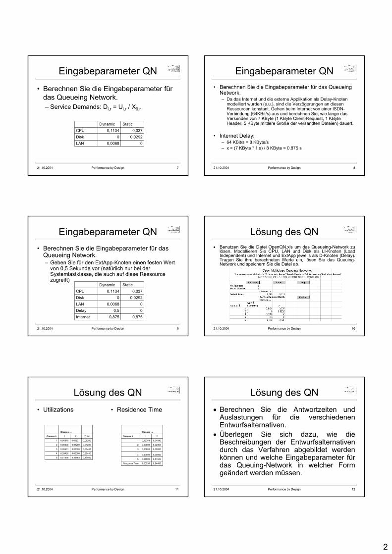
2
21.10.2004 Performance by Design 7
Eingabeparameter QN
• Berechnen Sie die Eingabeparameter für das Queueing Network.– Service Demands: Di,r = Ui,r / X0,r
00,0068LAN0,02920Disk
0,0370,1134CPUStaticDynamic
21.10.2004 Performance by Design 8
Eingabeparameter QN• Berechnen Sie die Eingabeparameter für das Queueing
Network.– Da das Internet und die externe Applikation als Delay-Knoten
modelliert wurden (s.u.), sind die Verzögerungen an diesen Ressourcen konstant. Gehen beim Internet von einer ISDN-Verbindung (64KBit/s) aus und berechnen Sie, wie lange das Versenden von 7 KByte (1 KByte Client-Request, 1 KByte Header, 5 KByte mittlere Größe der versandten Dateien) dauert.
• Internet Delay:– 64 KBit/s = 8 KByte/s– x = (7 KByte * 1 s) / 8 KByte = 0,875 s
21.10.2004 Performance by Design 9
Eingabeparameter QN• Berechnen Sie die Eingabeparameter für das
Queueing Network.– Geben Sie für den ExtApp-Knoten einen festen Wert
von 0,5 Sekunde vor (natürlich nur bei der Systemlastklasse, die auch auf diese Ressource zugreift)
00,0068LAN
0,8750,875Internet00,5Delay
0,02920Disk0,0370,1134CPU
StaticDynamic
21.10.2004 Performance by Design 10
Lösung des QN• Benutzen Sie die Datei OpenQN.xls um das Queueing-Network zu
lösen. Modellieren Sie CPU, LAN und Disk als LI-Knoten (LoadIndependent) und Internet und ExtApp jeweils als D-Knoten (Delay). Tragen Sie ihre berechneten Werte ein, lösen Sie das Queuing-Network und speichern Sie die Datei ab.
21.10.2004 Performance by Design 11
Lösung des QN• Utilizations • Residence Time
0,944861,50536Response Time
0,875000,875005
0,000000,500004
0,000000,006833
0,029550,000002
0,040300,123531
21Queues ↓
Classes→
0,875000,359630,515385
0,294500,000000,294504
0,004010,000000,004013
0,012000,012000,000002
0,082000,015210,066791
Total21Queues ↓
Classes→
21.10.2004 Performance by Design 12
Lösung des QN• Berechnen Sie die Antwortzeiten und
Auslastungen für die verschiedenen Entwurfsalternativen.
• Überlegen Sie sich dazu, wie die Beschreibungen der Entwurfsalternativen durch das Verfahren abgebildet werden können und welche Eingabeparameter für das Queuing-Network in welcher Form geändert werden müssen.
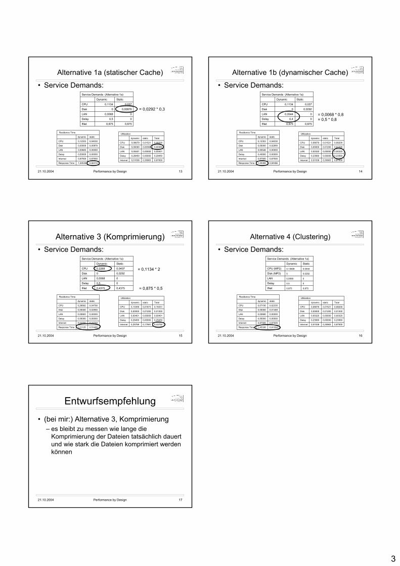
3
21.10.2004 Performance by Design 13
Alternative 1a (statischer Cache)
• Service Demands:
0,8750,875INet
00,5Delay
00,0068LAN
0,008760Disk
0,0370,1134CPU
StaticDynamic
Service Demands (Alternative 1a)
= 0,0292 * 0,3
0,924101,50536Response Time
0,875000,87500Internet
0,000000,50000Delay
0,000000,00683LAN
0,008790,00000Disk
0,040300,12353CPU
staticdynamic
Residence Time
0,875000,359630,51538Internet
0,294500,000000,29450Delay
0,004010,000000,00401LAN
0,003600,003600,00000Disk
0,082000,015210,06679CPU
Totalstaticdynamic
Utilization
21.10.2004 Performance by Design 14
Alternative 1b (dynamischer Cache)
• Service Demands:
0,8750,875INet
00,4Delay
00,0544LAN
0,02920Disk
0,0370,1134CPU
StaticDynamic
Service Demands (Alternative 1a)
= 0,0068 * 0,8= 0,5 * 0,8
0,944861,40399Response Time
0,875000,87500Internet
0,000000,40000Delay
0,000000,00546LAN
0,029550,00000Disk
0,040300,12353CPU
staticdynamic
Residence Time
0,875000,359630,51538Internet
0,235600,000000,23560Delay
0,003200,000000,00320LAN
0,012000,012000,00000Disk
0,082000,015210,06679CPU
Totalstaticdynamic
Utilization
21.10.2004 Performance by Design 15
Alternative 3 (Komprimierung)• Service Demands:
0,43750,4375INet
00,5Delay
00,0068LAN
0,02920Disk
0,04070,2268CPU
StaticDynamic
Service Demands (Alternative 1a)
= 0,1134 * 2
0,514951,21125Response Time
0,437500,43750Internet
0,000000,50000Delay
0,000000,00683LAN
0,029550,00000Disk
0,047900,26692CPU
staticdynamic
Residence Time
0,437500,179810,25769Internet
0,294500,000000,29450Delay
0,004010,000000,00401LAN
0,012000,012000,00000Disk
0,150310,016730,13359CPU
Totalstaticdynamic
Utilization
= 0,875 * 0,5
21.10.2004 Performance by Design 16
Alternative 4 (Clustering)
• Service Demands:
0,8750,875INet
00,5Delay
00,0068LAN
0,02920Disk (MP2)
0,04440,13608CPU (MP2)
StaticDynamic
Service Demands (Alternative 1a)
0,913041,45336Response Time
0,875000,87500Internet
0,000000,50000Delay
0,000000,00680LAN
0,014690,00000Disk
0,023350,07156CPU
staticdynamic
Residence Time
0,875000,359630,51538Internet
0,235600,000000,23560Delay
0,003200,000000,00320LAN
0,012000,012000,00000Disk
0,082000,015210,06679CPU
Totalstaticdynamic
Utilization
21.10.2004 Performance by Design 17
Entwurfsempfehlung
• (bei mir:) Alternative 3, Komprimierung– es bleibt zu messen wie lange die
Komprimierung der Dateien tatsächlich dauert und wie stark die Dateien komprimiert werden können
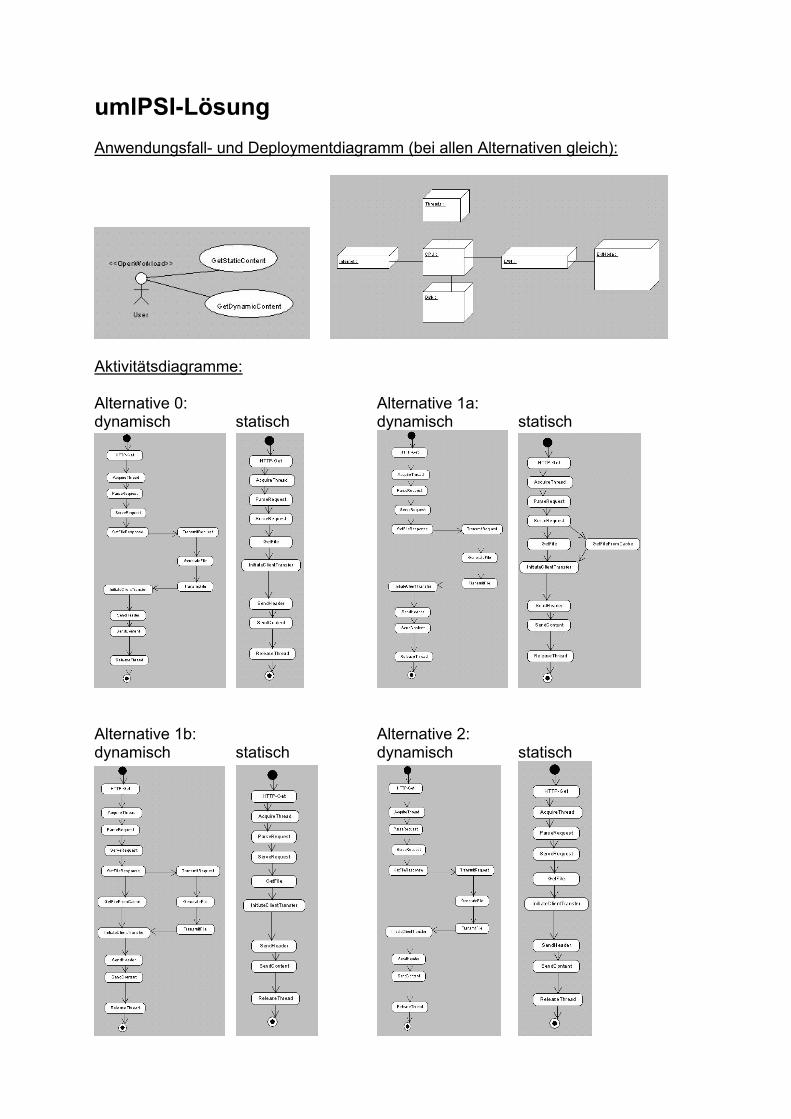
umlPSI-Lösung Anwendungsfall- und Deploymentdiagramm (bei allen Alternativen gleich):
Aktivitätsdiagramme: Alternative 0: Alternative 1a: dynamisch statisch dynamisch statisch
Alternative 1b: Alternative 2: dynamisch statisch dynamisch statisch
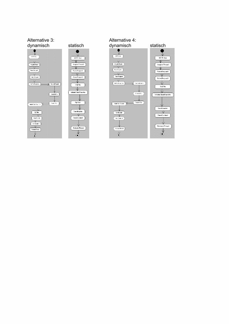
Alternative 3: Alternative 4: dynamisch statisch dynamisch statisch

lxviii
G. Rohdaten der Ergebnisse
Um eine nachtragliche, unabhangige Auswertung der Ergebnisse des Experimente zu ermogli-chen, wurden die Rohdaten jedes Teilnehmers in diese Ausarbeitung integriert. Fur jedes Verfah-ren werden die Durchlaufzeiten und Auslastungen fur jede Alternative angegeben. Beim SPE-Verfahren wird genau eine Durchlaufzeit angegeben, beim CP-Verfahren wird zusatzlich die Zeitangegeben, die auf jeder Ressource verbracht wird. Die Ausgaben des umlPSI-Werkzeugs zurSimulation der UML-Diagramme schließen sich an. Dabei wird fur jede Aktivitat eine Durch-laufzeit angegeben. Farblich hervorgehoben sind dort die Gesamtdurchlaufzeiten (blau) fur diebeiden Anwendungsfalle (statische bzw. dynamische Seitenabfragen) und die Ressourcenaus-lastungen (gelb). Diese Werte werden auch in den Auswertungsdiagrammen im Hauptteil derAusarbeitung verwendet.
lxix
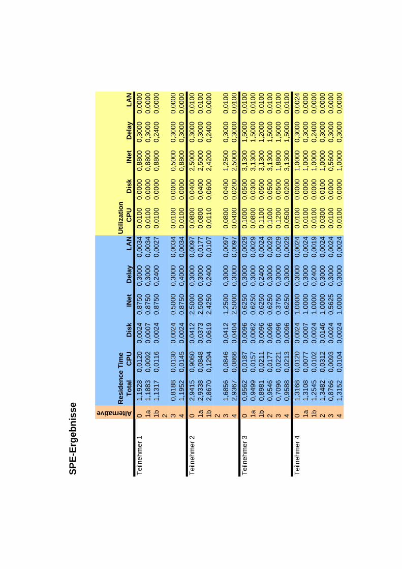
SPE-
Erge
bnis
se
Tota
lC
PUD
isk
INet
Del
ayLA
NC
PUD
isk
INet
Del
ayLA
NTe
ilneh
mer
10
1,19
280,
0120
0,00
240,
8750
0,30
000,
0034
0,01
000,
0000
0,88
000,
3000
0,00
001a
1,18
830,
0092
0,00
070,
8750
0,30
000,
0034
0,01
000,
0000
0,88
000,
3000
0,00
001b
1,13
170,
0116
0,00
240,
8750
0,24
000,
0027
0,01
000,
0000
0,88
000,
2400
0,00
002 3
0,81
880,
0130
0,00
240,
5000
0,30
000,
0034
0,01
000,
0000
0,50
000,
3000
0,00
004
1,19
520,
0145
0,00
240,
8750
0,40
000,
0034
0,01
000,
0000
0,88
000,
3000
0,00
00Te
ilneh
mer
20
2,94
150,
9060
0,04
122,
5000
0,30
000,
0097
0,08
000,
0400
2,50
000,
3000
0,01
001a
2,93
380,
0848
0,03
732,
5000
0,30
000,
0177
0,08
000,
0400
2,50
000,
3000
0,01
001b
2,86
700,
1294
0,06
192,
4250
0,24
000,
0107
0,01
100,
0600
2,42
000,
2400
0,00
002 3
1,68
560,
0846
0,04
121,
2500
0,30
000,
0097
0,08
000,
0400
1,25
000,
3000
0,01
004
2,93
670,
0866
0,04
042,
5000
0,30
000,
0097
0,04
000,
0200
2,50
000,
3000
0,01
00Te
ilneh
mer
30
0,95
620,
0187
0,00
960,
6250
0,30
000,
0029
0,10
000,
0500
3,13
001,
5000
0,01
001a
0,94
990,
0157
0,00
620,
6250
0,30
000,
0029
0,08
000,
0300
3,13
001,
5000
0,01
001b
0,89
810,
0211
0,00
960,
6250
0,24
000,
0024
0,11
000,
0500
3,13
001,
2000
0,01
002
0,95
460,
0177
0,00
960,
6250
0,30
000,
0029
0,10
000,
0500
3,13
001,
5000
0,01
003
0,70
960,
0221
0,00
960,
3750
0,30
000,
0029
0,12
000,
0500
1,88
001,
5000
0,01
004
0,95
880,
0213
0,00
960,
6250
0,30
000,
0029
0,05
000,
0200
3,13
001,
5000
0,01
00Te
ilneh
mer
40
1,31
680,
0120
0,00
241,
0000
0,30
000,
0024
0,01
000,
0000
1,00
000,
3000
0,00
241a
1,31
080,
0077
0,00
071,
0000
0,30
000,
0024
0,01
000,
0000
1,00
000,
3000
0,00
001b
1,25
450,
0102
0,00
241,
0000
0,24
000,
0019
0,01
000,
0000
1,00
000,
2400
0,00
002
1,34
820,
0312
0,01
461,
0000
0,30
000,
0024
0,03
000,
0100
1,00
000,
3000
0,00
003
0,8
766
0,00
930,
0024
0,56
250,
3000
0,00
240,
0100
0,00
000,
5600
0,30
000,
0000
4 1
,315
20,
0104
0,00
241,
0000
0,30
000,
0024
0,01
000,
0000
1,00
000,
3000
0,00
00
Res
iden
ce T
ime
Util
izat
ion
Alternative

Tota
lC
PUD
isk
INet
Del
ayLA
NC
PUD
isk
INet
Del
ayLA
NTe
ilneh
mer
50
1,55
030,
1633
0,08
461,
0000
0,30
000,
0024
0,14
000,
0800
1,00
000,
3000
0,00
001a
1,51
960,
1424
0,07
481,
0000
0,30
000,
0024
0,12
000,
0700
1,00
000,
3000
0,00
001b
1,48
680,
1603
0,08
461,
0000
0,24
000,
0019
0,14
000,
0800
1,00
000,
2400
0,00
002
1,54
770,
1607
0,08
461,
0000
0,30
000,
0024
0,14
000,
0800
1,00
000,
3000
0,00
003
1,29
790,
1629
0,08
460,
7500
0,30
000,
0024
0,14
000,
0800
0,75
000,
3000
0,00
004
1,53
230,
1488
0,08
121,
0000
0,30
000,
0024
0,07
000,
0400
1,00
000,
3000
0,00
00Te
ilneh
mer
60
1,84
760,
0351
0,01
201,
5000
0,30
000,
0005
0,00
000,
0000
0,02
000,
0000
0,00
001a
1,82
040,
0163
0,00
361,
5000
0,30
000,
0005
0,00
000,
0000
0,02
000,
0000
0,00
001b
1,78
260,
0302
0,01
201,
5000
0,20
000,
0004
0,00
000,
0000
0,02
000,
0000
0,00
002
1,8
428
0,03
030,
0120
1,50
000,
3000
0,00
050,
0000
0,00
000,
0200
0,00
000,
0000
3 1
,122
10,
0476
0,02
400,
7500
0,30
00 0
,000
50,
0000
0,00
000,
0100
0,00
000,
0000
4 1
,842
10,
0296
0,01
201,
5000
0,30
000,
0005
0,00
000,
0000
0,02
000,
0000
0,00
00Te
ilneh
mer
70
2,30
940,
0424
0,01
981,
1250
1,12
000,
0022
0,04
000,
0200
1,13
001,
2000
0,00
001a
2,30
300,
0376
0,01
821,
1250
1,12
000,
0022
0,04
000,
0200
1,13
001,
2000
0,00
001b
2,14
780,
0411
0,01
981,
1250
0,96
000,
0020
0,04
000,
0200
1,13
000,
9600
0,00
002
2,39
440,
0450
0,02
211,
1250
1,20
000,
0022
0,04
000,
0200
1,13
001,
2000
0,00
003
1,88
220,
0533
0,02
711,
0000
0,80
000,
0018
0,05
000,
0300
1,00
000,
8000
0,00
004
1,98
920,
0416
0,02
081,
1250
0,80
000,
0018
0,02
000,
0200
1,13
000,
8000
0,00
00Te
ilneh
mer
80
0,68
450,
0132
0,00
240,
3515
0,31
640,
0010
0,01
300,
0020
0,35
100,
3160
0,00
101a
0,62
000,
0132
0,00
070,
3515
0,25
880,
0010
0,01
300,
0010
0,35
100,
2590
0,00
101b
0,58
000,
0186
0,00
240,
3410
0,22
000,
0080
0,01
700,
0020
0,34
100,
2290
0,00
102 3
0,60
890,
0220
0,00
240,
2671
0,31
640,
0010
0,02
200,
0020
0,26
200,
3160
0,00
104
0,68
780,
0038
0,00
110,
3656
0,31
560,
0017
0,00
400,
0010
0,36
600,
3280
0,00
20
Alternative
Res
iden
ce T
ime
Util
izat
ion
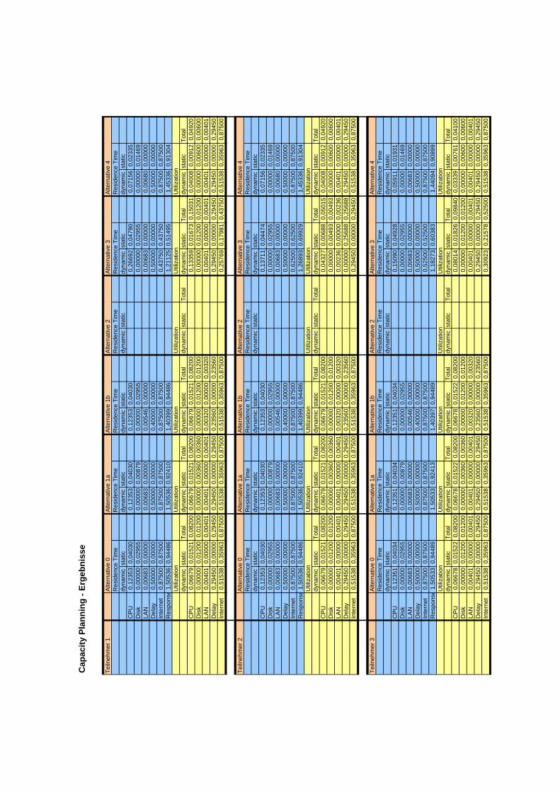
Cap
acity
Pla
nnin
g - E
rgeb
niss
e
Teiln
ehm
er 1
Res
iden
ce T
ime
Res
iden
ce T
ime
Res
iden
ce T
ime
Res
iden
ce T
ime
Res
iden
ce T
ime
Res
iden
ce T
ime
dyna
mic
stat
icdy
nam
icst
atic
dyna
mic
stat
icdy
nam
icst
atic
dyna
mic
stat
icdy
nam
icst
atic
CP
U0,
1235
30,
0403
00,
1235
30,
0403
00,
1235
30,
0403
00,
2669
20,
0479
00,
0715
60,
0233
5D
isk
0,00
000
0,02
955
0,00
000
0,00
879
0,00
000
0,02
955
0,00
000
0,02
955
0,00
000
0,01
469
LAN
0,00
683
0,00
000
0,00
683
0,00
000
0,00
546
0,00
000
0,00
683
0,00
000
0,00
680
0,00
000
Del
ay0,
5000
00,
0000
00,
5000
00,
0000
00,
4000
00,
0000
00,
5000
00,
0000
00,
5000
00,
0000
0In
tern
et0,
8750
00,
8750
00,
8750
00,
8750
00,
8750
00,
8750
00,
4375
00,
4375
00,
8750
00,
8750
0R
espo
nse
1,50
536
0,94
486
1,50
536
0,92
410
1,40
399
0,94
486
1,21
125
0,51
495
1,45
336
0,91
304
Util
izat
ion
Util
izat
ion
Util
izat
ion
Util
izat
ion
Util
izat
ion
Util
izat
ion
dyna
mic
stat
icTo
tal
dyna
mic
stat
icTo
tal
dyna
mic
stat
icTo
tal
dyna
mic
stat
icTo
tal
dyna
mic
stat
icTo
tal
dyna
mic
stat
icTo
tal
CP
U0,
0667
90,
0152
10,
0820
00,
0667
90,
0152
10,
0820
00,
0667
90,
0152
10,
0820
00,
1335
90,
0167
30,
1503
10,
0400
80,
0091
20,
0492
0D
isk
0,00
000
0,01
200
0,01
200
0,00
000
0,00
360
0,00
360
0,00
000
0,01
200
0,01
200
0,00
000
0,01
200
0,01
200
0,00
000
0,00
600
0,00
600
LAN
0,00
401
0,00
000
0,00
401
0,00
401
0,00
000
0,00
401
0,00
320
0,00
000
0,00
320
0,00
401
0,00
000
0,00
401
0,00
401
0,00
000
0,00
401
Del
ay0,
2945
00,
0000
00,
2945
00,
2945
00,
0000
00,
2945
00,
2356
00,
0000
00,
2356
00,
2945
00,
0000
00,
2945
00,
2945
00,
0000
00,
2945
0In
tern
et0,
5153
80,
3596
30,
8750
00,
5153
80,
3596
30,
8750
00,
5153
80,
3596
30,
8750
00,
2576
90,
1798
10,
4375
00,
5153
80,
3596
30,
8750
0
Teiln
ehm
er 2
Alte
rnat
ive
0A
ltern
ativ
e 1a
Alte
rnat
ive
1bA
ltern
ativ
e 2
Alte
rnat
ive
3A
ltern
ativ
e 4
Res
iden
ce T
ime
Res
iden
ce T
ime
Res
iden
ce T
ime
Res
iden
ce T
ime
Res
iden
ce T
ime
Res
iden
ce T
ime
dyna
mic
stat
icdy
nam
icst
atic
dyna
mic
stat
icdy
nam
icst
atic
dyna
mic
stat
icdy
nam
icst
atic
CP
U0,
1235
30,
0403
00,
1235
30,
0403
00,
1235
30,
0403
00,
1371
10,
0447
40,
0715
60,
0233
5D
isk
0,00
000
0,02
955
0,00
000
0,00
879
0,00
000
0,02
955
0,00
000
0,02
955
0,00
000
0,01
469
LAN
0,00
683
0,00
000
0,00
683
0,00
000
0,00
546
0,00
000
0,00
683
0,00
000
0,00
680
0,00
000
Del
ay0,
5000
00,
0000
00,
5000
00,
0000
00,
4000
00,
0000
00,
5000
00,
0000
00,
5000
00,
0000
0In
tern
et0,
8750
00,
8750
00,
8750
00,
8750
00,
8750
00,
8750
00,
6250
00,
6250
00,
8750
00,
8750
0R
espo
nse
1,50
536
0,94
486
1,50
536
0,92
410
1,40
399
0,94
486
1,26
893
0,69
929
1,45
336
0,91
304
Util
izat
ion
Util
izat
ion
Util
izat
ion
Util
izat
ion
Util
izat
ion
Util
izat
ion
dyna
mic
stat
icTo
tal
dyna
mic
stat
icTo
tal
dyna
mic
stat
icTo
tal
dyna
mic
stat
icTo
tal
dyna
mic
stat
icTo
tal
dyna
mic
stat
icTo
tal
CP
U0,
0667
90,
0152
10,
0820
00,
0667
90,
0152
10,
0820
00,
0667
90,
0152
10,
0820
00,
0432
70,
0068
80,
0501
50,
0400
80,
0091
20,
0492
0D
isk
0,00
000
0,01
200
0,01
200
0,00
000
0,00
360
0,00
360
0,00
000
0,01
200
0,01
200
0,00
000
0,00
493
0,00
493
0,00
000
0,00
600
0,00
600
LAN
0,00
401
0,00
000
0,00
401
0,00
401
0,00
000
0,00
401
0,00
320
0,00
000
0,00
320
0,00
236
0,00
000
0,00
236
0,00
401
0,00
000
0,00
401
Del
ay0,
2945
00,
0000
00,
2945
00,
2945
00,
0000
00,
2945
00,
2356
00,
0000
00,
2356
00,
0000
00,
2568
80,
2568
80,
2945
00,
0000
00,
2945
0In
tern
et0,
5153
80,
3596
30,
8750
00,
5153
80,
3596
30,
8750
00,
5153
80,
3596
30,
8750
00,
2945
00,
0000
00,
2945
00,
5153
80,
3596
30,
8750
0
Teiln
ehm
er 3
Alte
rnat
ive
0A
ltern
ativ
e 1a
Alte
rnat
ive
1bA
ltern
ativ
e 2
Alte
rnat
ive
3A
ltern
ativ
e 4
Res
iden
ce T
ime
Res
iden
ce T
ime
Res
iden
ce T
ime
Res
iden
ce T
ime
Res
iden
ce T
ime
Res
iden
ce T
ime
dyna
mic
stat
icdy
nam
icst
atic
dyna
mic
stat
icdy
nam
icst
atic
dyna
mic
stat
icdy
nam
icst
atic
CP
U0,
1235
10,
0403
40,
1235
10,
0403
40,
1235
10,
0403
40,
1509
00,
0492
80,
0591
10,
0193
1D
isk
0,00
000
0,02
955
0,00
000
0,00
879
0,00
000
0,02
955
0,00
000
0,02
955
0,00
000
0,01
469
LAN
0,00
683
0,00
000
0,00
683
0,00
000
0,00
546
0,00
000
0,00
683
0,00
000
0,00
683
0,00
000
Del
ay0,
5000
00,
0000
00,
5000
00,
0000
00,
4000
00,
0000
00,
5000
00,
0000
00,
5000
00,
0000
0In
tern
et0,
8750
00,
8750
00,
8750
00,
8750
00,
8750
00,
8750
00,
5250
00,
5250
00,
8750
00,
8750
0R
espo
nse
1,50
533
0,94
489
1,50
533
0,92
413
1,40
397
0,94
489
1,18
273
0,60
383
1,44
094
0,90
899
Util
izat
ion
Util
izat
ion
Util
izat
ion
Util
izat
ion
Util
izat
ion
Util
izat
ion
dyna
mic
stat
icTo
tal
dyna
mic
stat
icTo
tal
dyna
mic
stat
icTo
tal
dyna
mic
stat
icTo
tal
dyna
mic
stat
icTo
tal
dyna
mic
stat
icTo
tal
CP
U0,
0667
80,
0152
20,
0820
00,
0667
80,
0152
20,
0820
00,
0667
80,
0152
20,
0820
00,
0801
40,
0182
60,
0984
00,
0333
90,
0076
10,
0410
0D
isk
0,00
000
0,01
200
0,01
200
0,00
000
0,00
360
0,00
360
0,00
000
0,01
200
0,01
200
0,00
000
0,01
200
0,01
200
0,00
000
0,00
600
0,00
600
LAN
0,00
401
0,00
000
0,00
401
0,00
401
0,00
000
0,00
401
0,00
320
0,00
000
0,00
320
0,00
401
0,00
000
0,00
401
0,00
401
0,00
000
0,00
401
Del
ay0,
2945
00,
0000
00,
2945
00,
2945
00,
0000
00,
2945
00,
2356
00,
0000
00,
2356
00,
2945
00,
0000
00,
2945
00,
2945
00,
0000
00,
2945
0In
tern
et0,
5153
80,
3596
30,
8750
00,
5153
80,
3596
30,
8750
00,
5153
80,
3596
30,
8750
00,
3092
30,
2157
80,
5250
00,
5153
80,
3596
30,
8750
0
Alte
rnat
ive
3A
ltern
ativ
e 4
Alte
rnat
ive
0A
ltern
ativ
e 1a
Alte
rnat
ive
1bA
ltern
ativ
e 2
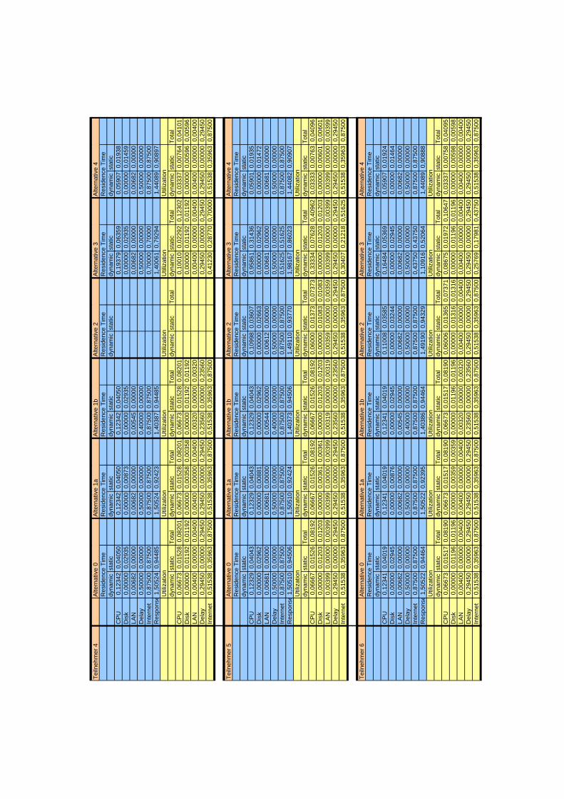
Teiln
ehm
er 4
Alte
rnat
ive
0A
ltern
ativ
e 1a
Alte
rnat
ive
1bA
ltern
ativ
e 2
Alte
rnat
ive
3A
ltern
ativ
e 4
Res
iden
ce T
ime
Res
iden
ce T
ime
Res
iden
ce T
ime
Res
iden
ce T
ime
Res
iden
ce T
ime
Res
iden
ce T
ime
dyna
mic
stat
icdy
nam
icst
atic
dyna
mic
stat
icdy
nam
icst
atic
dyna
mic
stat
icdy
nam
icst
atic
CP
U0,
1234
20,
0405
00,
1234
20,
0405
00,
1234
20,
0405
00,
1937
90,
0635
90,
0590
70,
0193
8D
isk
0,00
000
0,02
935
0,00
000
0,00
873
0,00
000
0,02
935
0,00
000
0,02
935
0,00
000
0,01
459
LAN
0,00
682
0,00
000
0,00
682
0,00
000
0,00
545
0,00
000
0,00
682
0,00
000
0,00
682
0,00
000
Del
ay0,
5000
00,
0000
00,
5000
00,
0000
00,
4000
00,
0000
00,
5000
00,
0000
00,
5000
00,
0000
0In
tern
et0,
8750
00,
8750
00,
8750
00,
8750
00,
8750
00,
8750
00,
7000
00,
7000
00,
8750
00,
8750
0R
espo
nse
1,50
524
0,94
485
1,50
524
0,92
423
1,40
387
0,94
485
1,40
061
0,79
294
1,44
089
0,90
897
Util
izat
ion
Util
izat
ion
Util
izat
ion
Util
izat
ion
Util
izat
ion
Util
izat
ion
dyna
mic
stat
icTo
tal
dyna
mic
stat
icTo
tal
dyna
mic
stat
icTo
tal
dyna
mic
stat
icTo
tal
dyna
mic
stat
icTo
tal
dyna
mic
stat
icTo
tal
CP
U0,
0667
30,
0152
80,
0820
10,
0667
30,
0152
80,
0820
10,
0667
30,
0152
80,
0820
10,
1001
00,
0229
20,
1230
20,
0333
70,
0076
40,
0410
1D
isk
0,00
000
0,01
192
0,01
192
0,00
000
0,00
358
0,00
358
0,00
000
0,01
192
0,01
192
0,00
000
0,01
192
0,01
192
0,00
000
0,00
596
0,00
596
LAN
0,00
400
0,00
000
0,00
400
0,00
400
0,00
000
0,00
400
0,00
320
0,00
000
0,00
320
0,00
400
0,00
000
0,00
400
0,00
400
0,00
000
0,00
400
Del
ay0,
2945
00,
0000
00,
2945
00,
2945
00,
0000
00,
2945
00,
2356
00,
0000
00,
2356
00,
2945
00,
0000
00,
2945
00,
2945
00,
0000
00,
2945
0In
tern
et0,
5153
80,
3596
30,
8750
00,
5153
80,
3596
30,
8750
00,
5153
80,
3596
30,
8750
00,
4123
00,
2877
00,
7000
00,
5153
80,
3596
30,
8750
0
Teiln
ehm
er 5
Alte
rnat
ive
0A
ltern
ativ
e 1a
Alte
rnat
ive
1bA
ltern
ativ
e 2
Alte
rnat
ive
3A
ltern
ativ
e 4
Res
iden
ce T
ime
Res
iden
ce T
ime
Res
iden
ce T
ime
Res
iden
ce T
ime
Res
iden
ce T
ime
Res
iden
ce T
ime
dyna
mic
stat
icdy
nam
icst
atic
dyna
mic
stat
icdy
nam
icst
atic
dyna
mic
stat
icdy
nam
icst
atic
CP
U0,
1232
90,
0404
30,
1232
90,
0404
30,
1232
90,
0404
30,
1099
80,
0360
70,
9586
10,
3143
60,
0590
10,
0193
5D
isk
0,00
000
0,02
962
0,00
000
0,00
881
0,00
000
0,02
962
0,00
000
0,02
663
0,00
000
0,02
962
0,00
000
0,01
472
LAN
0,00
681
0,00
000
0,00
681
0,00
000
0,00
544
0,00
000
0,00
612
0,00
000
0,00
681
0,00
000
0,00
681
0,00
000
Del
ay0,
5000
00,
0000
00,
5000
00,
0000
00,
4000
00,
0000
00,
5000
00,
0000
00,
5000
00,
0000
00,
5000
00,
0000
0In
tern
et0,
8750
00,
8750
00,
8750
00,
8750
00,
8750
00,
8750
00,
8750
00,
8750
00,
5162
50,
5162
50,
8750
00,
8750
0R
espo
nse
1,50
510
0,94
506
1,50
510
0,92
424
1,40
373
0,94
506
1,49
110
0,93
770
1,98
167
0,86
023
1,44
082
0,90
907
Util
izat
ion
Util
izat
ion
Util
izat
ion
Util
izat
ion
Util
izat
ion
Util
izat
ion
dyna
mic
stat
icTo
tal
dyna
mic
stat
icTo
tal
dyna
mic
stat
icTo
tal
dyna
mic
stat
icTo
tal
dyna
mic
stat
icTo
tal
dyna
mic
stat
icTo
tal
CP
U0,
0666
70,
0152
60,
0819
20,
0666
70,
0152
60,
0819
20,
0666
70,
0152
60,
0819
20,
0600
00,
0137
30,
0737
30,
3333
40,
0762
80,
4096
20,
0333
30,
0076
30,
0409
6D
isk
0,00
000
0,01
203
0,01
203
0,00
000
0,00
361
0,00
361
0,00
000
0,01
203
0,01
203
0,00
000
0,01
083
0,01
083
0,00
000
0,01
203
0,01
203
0,00
000
0,00
601
0,00
601
LAN
0,00
399
0,00
000
0,00
399
0,00
399
0,00
000
0,00
399
0,00
319
0,00
000
0,00
319
0,00
359
0,00
000
0,00
359
0,00
399
0,00
000
0,00
399
0,00
399
0,00
000
0,00
399
Del
ay0,
2945
00,
0000
00,
2945
00,
2945
00,
0000
00,
2945
00,
2356
00,
0000
00,
2356
00,
2945
00,
0000
00,
2945
00,
2945
00,
0000
00,
2945
00,
2945
00,
0000
00,
2945
0In
tern
et0,
5153
80,
3596
30,
8750
00,
5153
80,
3596
30,
8750
00,
5153
80,
3596
30,
8750
00,
5153
80,
3596
30,
8750
00,
3040
70,
2121
80,
5162
50,
5153
80,
3596
30,
8750
0
Teiln
ehm
er 6
Alte
rnat
ive
0A
ltern
ativ
e 1a
Alte
rnat
ive
1bA
ltern
ativ
e 2
Alte
rnat
ive
3A
ltern
ativ
e 4
Res
iden
ce T
ime
Res
iden
ce T
ime
Res
iden
ce T
ime
Res
iden
ce T
ime
Res
iden
ce T
ime
Res
iden
ce T
ime
dyna
mic
stat
icdy
nam
icst
atic
dyna
mic
stat
icdy
nam
icst
atic
dyna
mic
stat
icdy
nam
icst
atic
CP
U0,
1234
10,
0401
90,
1234
10,
0401
90,
1234
10,
0401
90,
1100
80,
0358
50,
1648
40,
0536
90,
0590
70,
0192
4D
isk
0,00
000
0,02
945
0,00
000
0,00
876
0,00
000
0,02
945
0,00
000
0,03
244
0,00
000
0,02
945
0,00
000
0,01
464
LAN
0,00
682
0,00
000
0,00
682
0,00
000
0,00
545
0,00
000
0,00
682
0,00
000
0,00
682
0,00
000
0,00
682
0,00
000
Del
ay0,
5000
00,
0000
00,
5000
00,
0000
00,
4000
00,
0000
00,
5000
00,
0000
00,
5000
00,
0000
00,
5000
00,
0000
0In
tern
et0,
8750
00,
8750
00,
8750
00,
8750
00,
8750
00,
8750
00,
8750
00,
8750
00,
4375
00,
4375
00,
8750
00,
8750
0R
espo
nse
1,50
522
0,94
464
1,50
522
0,92
395
1,40
386
0,94
464
1,49
190
0,94
329
1,10
916
0,52
064
1,44
089
0,90
888
Util
izat
ion
Util
izat
ion
Util
izat
ion
Util
izat
ion
Util
izat
ion
Util
izat
ion
dyna
mic
stat
icTo
tal
dyna
mic
stat
icTo
tal
dyna
mic
stat
icTo
tal
dyna
mic
stat
icTo
tal
dyna
mic
stat
icTo
tal
dyna
mic
stat
icTo
tal
CP
U0,
0667
30,
0151
70,
0819
00,
0667
30,
0151
70,
0819
00,
0667
30,
0151
70,
0819
00,
0600
60,
0136
50,
0737
10,
0867
50,
0197
20,
1064
70,
0333
70,
0075
80,
0409
5D
isk
0,00
000
0,01
196
0,01
196
0,00
000
0,00
359
0,00
359
0,00
000
0,01
196
0,01
196
0,00
000
0,01
316
0,01
316
0,00
000
0,01
196
0,01
196
0,00
000
0,00
598
0,00
598
LAN
0,00
400
0,00
000
0,00
400
0,00
400
0,00
000
0,00
400
0,00
320
0,00
000
0,00
320
0,00
400
0,00
000
0,00
400
0,00
400
0,00
000
0,00
400
0,00
400
0,00
000
0,00
400
Del
ay0,
2945
00,
0000
00,
2945
00,
2945
00,
0000
00,
2945
00,
2356
00,
0000
00,
2356
00,
2945
00,
0000
00,
2945
00,
2945
00,
0000
00,
2945
00,
2945
00,
0000
00,
2945
0In
tern
et0,
5153
80,
3596
30,
8750
00,
5153
80,
3596
30,
8750
00,
5153
80,
3596
30,
8750
00,
5153
80,
3596
30,
8750
00,
2576
90,
1798
10,
4375
00,
5153
80,
3596
30,
8750
0
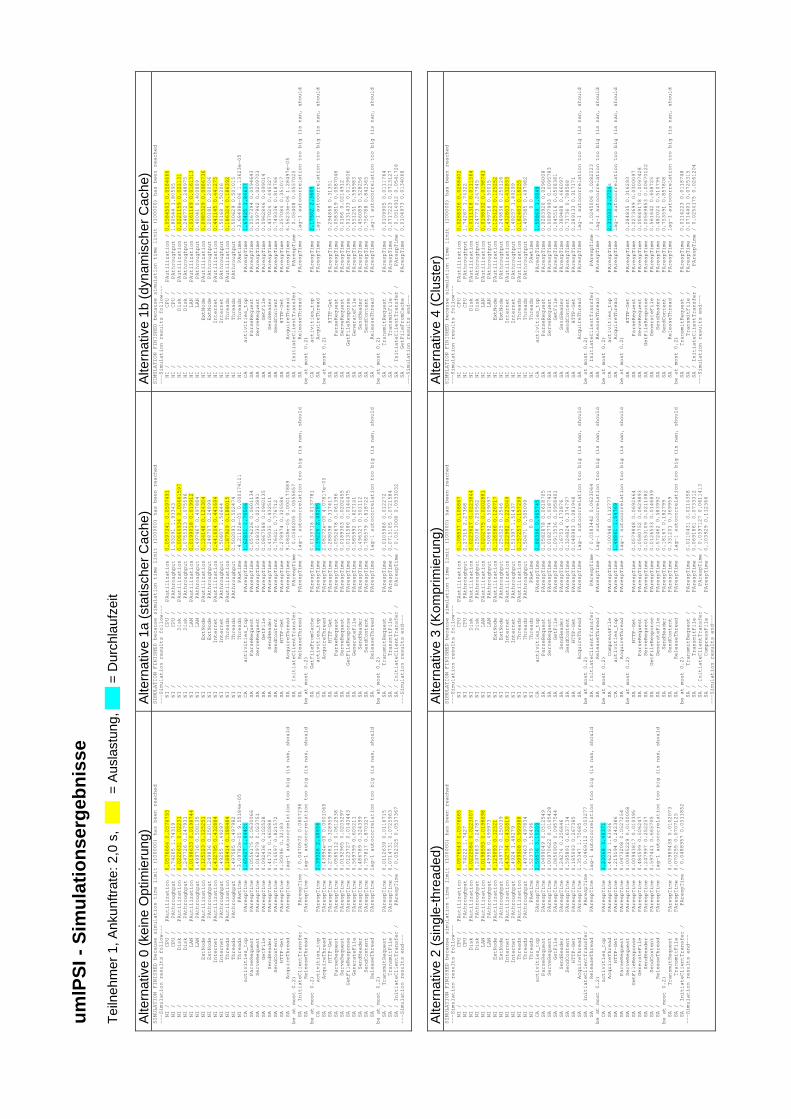
umlP
SI -
Sim
ulat
ions
erge
bnis
se
Teiln
ehm
er 1
, Ank
unftr
ate:
2,0
s,
___
= A
usla
stun
g, _
__ =
Dur
chla
ufze
it A
ltern
ativ
e 0
(kei
ne O
ptim
ieru
ng)
Alte
rnat
ive
1a (s
tatis
cher
Cac
he)
Alte
rnat
ive
1b (d
ynam
isch
er C
ache
) SIMULATION FINISHED because simulation time limit (100000) has been reached
---Simulation results follow---
NI / CPU / PAutilization / 0.0576664 0.0576793
NI / CPU / PAthroughput / 1.74265 1.74319
NI / Disk / PAutilization / 0.0222631 0.02231
NI / Disk / PAthroughput / 0.247726 0.247931
NI / LAN / PAutilization / 0.0198633 0.0198744
NI / LAN / PAthroughput / 0.499716 0.500135
NI / ExtNode / PAutilization / 0.125123 0.125251
NI / ExtNode / PAthroughput / 0.249836 0.250122
NI / Internet / PAutilization / 0.432795 0.432884
NI / Internet / PAthroughput / 1.49255 1.49297
NI / Threads / PAutilization / 0.188414 0.188484
NI / Threads / PAthroughput / 0.497585 0.497982
NI / Threads / PAwtime / -3.09782e-05 9.55184e-05
CA / activities_top / PArespTime / 1.65427 1.84421
SA / ParseRequest / PArespTime / 0.0556175 0.0630066
SA / ServeRequest / PArespTime / 0.0162979 0.023751
SA / GetFile / PArespTime / 0.092436 0.102528
SA / SendHeader / PArespTime / 0.41721 0.460888
SA / SendContent / PArespTime / 0.714597 0.821572
SA / HTTP-Get / PArespTime / 0.30096 0.32183
SA / AcquireThread / PArespTime / lag-1 autocorrelation too big (is nan, should
be at most 0.2)
SA / InitiateClientTransfer / PArespTime / 0.0470572 0.0607296
SA / ReleaseThread / PArespTime / lag-1 autocorrelation too big (is nan, should
be at most 0.2)
CA / activities_top / PArespTime / 2.39326 2.48656
SA / AcquireThread / PArespTime / 5.43894e-05 0.0001065
SA / HTTP-Get / PArespTime / 0.278981 0.328959
SA / ParseRequest / PArespTime / 0.0565112 0.0612538
SA / ServeRequest / PArespTime / 0.0192965 0.0205297
SA / GetFileResponse / PArespTime / 0.0123727 0.0143443
SA / GenerateFile / PArespTime / 0.569799 0.605211
SA / SendHeader / PArespTime / 0.486789 0.524399
SA / SendContent / PArespTime / 0.757817 0.870327
SA / ReleaseThread / PArespTime / lag-1 autocorrelation too big (is nan, should
be at most 0.2)
SA / TransmitRequest / PArespTime / 0.0112639 0.0116715
SA / TransmitFile / PArespTime / 0.0714731 0.0725963
SA / InitiateClientTransfer / PArespTime / 0.052325 0.0537367
---Simulation results end---
SIMULATION FINISHED because simulation time limit (100000) has been reached
---Simulation results follow---
NI / CPU / PAutilization / 0.0597341 0.0597491
NI / CPU / PAthroughput / 1.93291 1.93343
NI / Disk / PAutilization / 0.00660934 0.00661597
NI / Disk / PAthroughput / 0.0755323 0.075596
NI / LAN / PAutilization / 0.0199018 0.019912
NI / LAN / PAthroughput / 0.497467 0.497884
NI / ExtNode / PAutilization / 0.124148 0.124304
NI / ExtNode / PAthroughput / 0.248707 0.24899
NI / Internet / PAutilization / 0.441604 0.441694
NI / Internet / PAthroughput / 1.50607 1.50644
NI / Threads / PAutilization / 0.187929 0.188015
NI / Threads / PAthroughput / 0.502091 0.502474
NI / Threads / PAwtime / -4.21102e-05 0.000174111
CA / activities_top / PArespTime / 1.62851 1.70566
SA / ParseRequest / PArespTime / 0.0576226 0.0601134
SA / ServeRequest / PArespTime / 0.018335 0.0213891
SA / GetFile / PArespTime / 0.0867588 0.0960135
SA / SendHeader / PArespTime / 0.415035 0.432511
SA / SendContent / PArespTime / 0.76421 0.776712
SA / HTTP-Get / PArespTime / 0.278974 0.325586
SA / AcquireThread / PArespTime / 9.0848e-05 0.000177889
SA / InitiateClientTransfer / PArespTime / 0.0540205 0.0555657
SA / ReleaseThread / PArespTime / lag-1 autocorrelation too big (is nan, should
be at most 0.2)
SA / GetFileFromCache / PArespTime / 0.0135716 0.0137781
CA / activities_top / PArespTime / 2.39226 2.48285
SA / AcquireThread / PArespTime / 2.08272e-05 4.07817e-05
SA / HTTP-Get / PArespTime / 0.288098 0.317417
SA / ParseRequest / PArespTime / 0.0552678 0.061396
SA / ServeRequest / PArespTime / 0.0189303 0.0202455
SA / GetFileResponse / PArespTime / 0.0131586 0.0144475
SA / GenerateFile / PArespTime / 0.585992 0.627141
SA / SendHeader / PArespTime / 0.496327 0.501112
SA / SendContent / PArespTime / 0.785579 0.818722
SA / ReleaseThread / PArespTime / lag-1 autocorrelation too big (is nan, should
be at most 0.2)
SA / TransmitRequest / PArespTime / 0.0105986 0.012272
SA / TransmitFile / PArespTime / 0.0715105 0.0721584
SA / InitiateClientTransfer / PArespTime / 0.0513008 0.0533032
---Simulation results end---
SIMULATION FINISHED because simulation time limit (100000) has been reached
---Simulation results follow---
NI / CPU / PAutilization / 0.0584503 0.0584666
NI / CPU / PAthroughput / 1.80544 1.80595
NI / Disk / PAutilization / 0.0221159 0.022131
NI / Disk / PAthroughput / 0.248772 0.248975
NI / LAN / PAutilization / 0.0161169 0.0161313
NI / LAN / PAthroughput / 0.40041 0.400889
NI / ExtNode / PAutilization / 0.0985329 0.0986736
NI / ExtNode / PAthroughput / 0.200181 0.200506
NI / Internet / PAutilization / 0.441145 0.441275
NI / Internet / PAthroughput / 1.50168 1.50206
NI / Threads / PAutilization / 0.186324 0.186392
NI / Threads / PAthroughput / 0.500629 0.501015
NI / Threads / PAwtime / -3.68498e-06 1.13623e-05
CA / activities_top / PArespTime / 1.67425 1.84637
SA / ParseRequest / PArespTime / 0.0567394 0.0594643
SA / ServeRequest / PArespTime / 0.0197942 0.0209703
SA / GetFile / PArespTime / 0.0962846 0.099014
SA / SendHeader / PArespTime / 0.437024 0.445327
SA / SendContent / PArespTime / 0.749336 0.818766
SA / HTTP-Get / PArespTime / 0.257084 0.351017
SA / AcquireThread / PArespTime / 6.56233e-06 1.28497e-05
SA / InitiateClientTransfer / PArespTime / 0.05408 0.0557025
SA / ReleaseThread / PArespTime / lag-1 autocorrelation too big (is nan, should
be at most 0.2)
CA / activities_top / PArespTime / 2.17502 2.3605
SA / AcquireThread / PArespTime / lag-1 autocorrelation too big (is nan, should
be at most 0.2)
SA / HTTP-Get / PArespTime / 0.294868 0.31351
SA / ParseRequest / PArespTime / 0.0583819 0.0587046
SA / ServeRequest / PArespTime / 0.0186 0.0214912
SA / GetFileResponse / PArespTime / 0.0131433 0.0139606
SA / GenerateFile / PArespTime / 0.551251 0.595983
SA / SendHeader / PArespTime / 0.456089 0.528256
SA / SendContent / PArespTime / 0.756788 0.842365
SA / ReleaseThread / PArespTime / lag-1 autocorrelation too big (is nan, should
be at most 0.2)
SA / TransmitRequest / PArespTime / 0.0109905 0.0111764
SA / TransmitFile / PArespTime / 0.0717223 0.0723127
SA / InitiateClientTransfer / PArespTime / 0.0514912 0.0541726
SA / GetFileFromCache / PArespTime / 0.0104973 0.0134068
---Simulation results end---
Alte
rnat
ive
2 (s
ingl
e-th
read
ed)
Alte
rnat
ive
3 (K
ompr
imie
rung
) A
ltern
ativ
e 4
(Clu
ster
) SIMULATION FINISHED because simulation time limit (100000) has been reached
---Simulation results follow---
NI / CPU / PAutilization / 0.0576543 0.0576665
NI / CPU / PAthroughput / 1.74222 1.7427
NI / Disk / PAutilization / 0.0222584 0.0223007
NI / Disk / PAthroughput / 0.247683 0.24787
NI / LAN / PAutilization / 0.0198593 0.0198698
NI / LAN / PAthroughput / 0.49958 0.499973
NI / ExtNode / PAutilization / 0.125093 0.12521
NI / ExtNode / PAthroughput / 0.249772 0.250039
NI / Internet / PAutilization / 0.432734 0.432819
NI / Internet / PAthroughput / 1.4924 1.49279
NI / Threads / PAutilization / 0.999908 0.999988
NI / Threads / PAthroughput / 0.497463 0.497834
NI / Threads / PAwtime / 1.52379 1.56496
CA / activities_top / PArespTime / 2.59576 3.10209
SA / ParseRequest / PArespTime / 0.0499049 0.0512549
SA / ServeRequest / PArespTime / 0.00970622 0.0105428
SA / GetFile / PArespTime / 0.0850909 0.0957544
SA / SendHeader / PArespTime / 0.24274 0.256846
SA / SendContent / PArespTime / 0.595891 0.637134
SA / HTTP-Get / PArespTime / 0.185093 0.267385
SA / AcquireThread / PArespTime / 1.35347 1.75685
SA / InitiateClientTransfer / PArespTime / 0.0469112 0.053277
SA / ReleaseThread / PArespTime / lag-1 autocorrelation too big (is nan, should
be at most 0.2)
CA / activities_top / PArespTime / 3.23068 3.48371
SA / AcquireThread / PArespTime / 1.46232 1.63936
SA / HTTP-Get / PArespTime / 0.215194 0.242386
SA / ParseRequest / PArespTime / 0.0473208 0.0527254
SA / ServeRequest / PArespTime / 0.00985229 0.0100058
SA / GetFileResponse / PArespTime / 0.00943817 0.010395
SA / GenerateFile / PArespTime / 0.484599 0.506247
SA / SendHeader / PArespTime / 0.247997 0.252257
SA / SendContent / PArespTime / 0.597441 0.665705
SA / ReleaseThread / PArespTime / lag-1 autocorrelation too big (is nan, should
be at most 0.2)
SA / TransmitRequest / PArespTime / 0.00989438 0.0102073
SA / TransmitFile / PArespTime / 0.070255 0.0707125
SA / InitiateClientTransfer / PArespTime / 0.0488957 0.0511852
---Simulation results end---
SIMULATION FINISHED because simulation time limit (100000) has been reached
---Simulation results follow---
NI / CPU / PAutilization / 0.108837 0.108867
NI / CPU / PAthroughput / 2.27315 2.27368
NI / Disk / PAutilization / 0.0223627 0.0223844
NI / Disk / PAthroughput / 0.25036 0.250562
NI / LAN / PAutilization / 0.0202775 0.0202881
NI / LAN / PAthroughput / 0.508692 0.509097
NI / ExtNode / PAutilization / 0.126586 0.126717
NI / ExtNode / PAthroughput / 0.254325 0.2546
NI / Internet / PAutilization / 0.222982 0.223049
NI / Internet / PAthroughput / 1.51397 1.51437
NI / Threads / PAutilization / 0.157257 0.157299
NI / Threads / PAthroughput / 0.50471 0.505099
NI / Threads / PAwtime / 0 0
CA / activities_top / PArespTime / 0.88396 0.965745
SA / ParseRequest / PArespTime / 0.0582878 0.0618705
SA / ServeRequest / PArespTime / 0.0182774 0.0187421
SA / GetFile / PArespTime / 0.0913536 0.0958401
SA / SendHeader / PArespTime / 0.16753 0.172876
SA / SendContent / PArespTime / 0.324824 0.374797
SA / HTTP-Get / PArespTime / 0.048983 0.081948
SA / AcquireThread / PArespTime / lag-1 autocorrelation too big (is nan, should
be at most 0.2)
SA / InitiateClientTransfer / PArespTime / 0.0583442 0.0623064
SA / ReleaseThread / PArespTime / lag-1 autocorrelation too big (is nan, should
be at most 0.2)
SA / CompressFile / PArespTime / 0.100948 0.112777
CA / activities_top / PArespTime / 1.48861 1.54769
SA / AcquireThread / PArespTime / lag-1 autocorrelation too big (is nan, should
be at most 0.2)
SA / HTTP-Get / PArespTime / 0.0579848 0.0692664
SA / ParseRequest / PArespTime / 0.0580752 0.0629893
SA / ServeRequest / PArespTime / 0.0153109 0.0211082
SA / GetFileResponse / PArespTime / 0.0126533 0.0146839
SA / GenerateFile / PArespTime / 0.572462 0.583992
SA / SendHeader / PArespTime / 0.18167 0.182799
SA / SendContent / PArespTime / 0.331201 0.369959
SA / ReleaseThread / PArespTime / lag-1 autocorrelation too big (is nan, should
be at most 0.2)
SA / TransmitRequest / PArespTime / 0.0110431 0.0114358
SA / TransmitFile / PArespTime / 0.0691861 0.0733312
SA / InitiateClientTransfer / PArespTime / 0.0597127 0.0611413
SA / CompressFile / PArespTime / 0.103929 0.112366
---Simulation results end---
SIMULATION FINISHED because simulation time limit (100000) has been reached
---Simulation results follow---
NI / CPU / PAutilization / 0.0288336 0.0288402
NI / CPU / PAthroughput / 1.74267 1.74322
NI / Disk / PAutilization / 0.0111318 0.0111564
NI / Disk / PAthroughput / 0.24773 0.247945
NI / LAN / PAutilization / 0.0198632 0.0198743
NI / LAN / PAthroughput / 0.499716 0.50015
NI / ExtNode / PAutilization / 0.125123 0.125252
NI / ExtNode / PAthroughput / 0.249836 0.250126
NI / Internet / PAutilization / 0.432803 0.432893
NI / Internet / PAthroughput / 1.49257 1.49299
NI / Threads / PAutilization / 0.182483 0.18255
NI / Threads / PAthroughput / 0.497585 0.497982
NI / Threads / PAwtime / 0 0
CA / activities_top / PArespTime / 1.50869 1.6848
SA / ParseRequest / PArespTime / 0.0283926 0.0296008
SA / ServeRequest / PArespTime / 0.00897993 0.0095783
SA / GetFile / PArespTime / 0.045516 0.0508381
SA / SendHeader / PArespTime / 0.389488 0.466097
SA / SendContent / PArespTime / 0.71736 0.788588
SA / HTTP-Get / PArespTime / 0.289133 0.317171
SA / AcquireThread / PArespTime / lag-1 autocorrelation too big (is nan, should
be at most 0.2)
SA / InitiateClientTransfer / PArespTime / 0.0245006 0.0282523
SA / ReleaseThread / PArespTime / lag-1 autocorrelation too big (is nan, should
be at most 0.2)
CA / activities_top / PArespTime / 2.31033 2.3724s
SA / AcquireThread / PArespTime / lag-1 autocorrelation too big (is nan, should
be at most 0.2)
SA / HTTP-Get / PArespTime / 0.284835 0.316293
SA / ParseRequest / PArespTime / 0.0273699 0.0300097
SA / ServeRequest / PArespTime / 0.00849178 0.0097428
SA / GetFileResponse / PArespTime / 0.00589853 0.00670122
SA / GenerateFile / PArespTime / 0.561642 0.608725
SA / SendHeader / PArespTime / 0.482024 0.510796
SA / SendContent / PArespTime / 0.753591 0.857808
SA / ReleaseThread / PArespTime / lag-1 autocorrelation too big (is nan, should
be at most 0.2)
SA / TransmitRequest / PArespTime / 0.0114223 0.0118748
SA / TransmitFile / PArespTime / 0.0714401 0.0725315
SA / InitiateClientTransfer / PArespTime / 0.0254175 0.0261204
---Simulation results end---
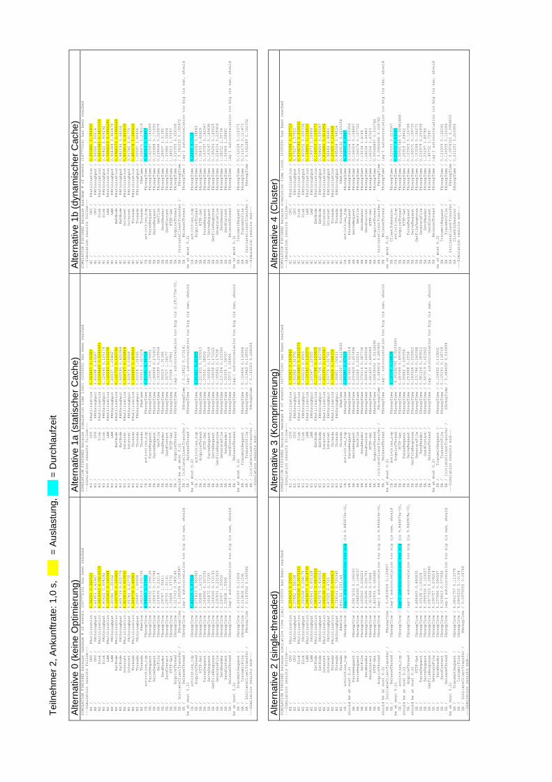
Teiln
ehm
er 2
, Ank
unftr
ate:
1,0
s,
___
= A
usla
stun
g, _
__ =
Dur
chla
ufze
it A
ltern
ativ
e 0
(kei
ne O
ptim
ieru
ng)
Alte
rnat
ive
1a (s
tatis
cher
Cac
he)
Alte
rnat
ive
1b (d
ynam
isch
er C
ache
) SIMULATION FINISHED because maximum # of events (16777216) has been reached
---Simulation results follow---
NI / CPU / PAutilization / 0.36251 0.362522
NI / CPU / PAthroughput / 3.61953 3.61967
NI / Disk / PAutilization / 0.0810463 0.0810559
NI / Disk / PAthroughput / 0.40422 0.404292
NI / LAN / PAutilization / 0.120363 0.120368
NI / LAN / PAthroughput / 1.20344 1.20352
NI / ExtNode / PAutilization / 0.120785 0.120802
NI / ExtNode / PAthroughput / 0.601719 0.601779
NI / Internet / PAutilization / 0.823813 0.823832
NI / Internet / PAthroughput / 3.01761 3.01772
NI / Threads / PAutilization / 0.469778 0.46983
NI / Threads / PAthroughput / 1.00597 1.00606
NI / Threads / PAwtime / 0.282019 0.291739
CA / activities_top / PArespTime / 4.89465 5.07582
SA / ParseRequest / PArespTime / 0.165332 0.166126
SA / ServeRequest / PArespTime / 0.165473 0.172784
SA / GetFile / PArespTime / 0.216935 0.22218
SA / SendHeader / PArespTime / 1.29767 1.30411
SA / SendContent / PArespTime / 1.29733 1.35141
SA / HTTP-Get / PArespTime / 1.33658 1.37732
SA / AcquireThread / PArespTime / 0.213743 0.349146
SA / InitiateClientTransfer / PArespTime / 0.165284 0.168947
SA / ReleaseThread / PArespTime / lag-1 autocorrelation too big (is nan, should
be at most 0.2)
CA / activities_top / PArespTime / 5.42115 5.87354
SA / AcquireThread / PArespTime / 0.171413 0.385463
SA / HTTP-Get / PArespTime / 1.30898 1.41723
SA / ParseRequest / PArespTime / 0.166066 0.167252
SA / ServeRequest / PArespTime / 0.164872 0.17295
SA / GetFileResponse / PArespTime / 0.166346 0.172193
SA / GenerateFile / PArespTime / 0.230931 0.231929
SA / SendHeader / PArespTime / 1.29397 1.35652
SA / SendContent / PArespTime / 1.50838 1.5906
SA / ReleaseThread / PArespTime / lag-1 autocorrelation too big (is nan, should
be at most 0.2)
SA / TransmitRequest / PArespTime / 0.115193 0.11606
SA / TransmitFile / PArespTime / 0.113836 0.11541
SA / InitiateClientTransfer / PArespTime / 0.163502 0.165582
---Simulation results end---
SIMULATION FINISHED because simulation time limit (100000) has been reached
---Simulation results follow---
NI / CPU / PAutilization / 0.363807 0.36384
NI / CPU / PAthroughput / 3.63248 3.63287
NI / Disk / PAutilization / 0.0244669 0.0244991
NI / Disk / PAthroughput / 0.124065 0.124179
NI / LAN / PAutilization / 0.120283 0.120298
NI / LAN / PAthroughput / 1.20437 1.20462
NI / ExtNode / PAutilization / 0.120733 0.120782
NI / ExtNode / PAthroughput / 0.602185 0.602364
NI / Internet / PAutilization / 0.826767 0.826816
NI / Internet / PAthroughput / 3.02973 3.03004
NI / Threads / PAutilization / 0.469459 0.469569
NI / Threads / PAthroughput / 1.01018 1.01045
NI / Threads / PAwtime / 0.30912 0.327378
CA / activities_top / PArespTime / 4.81081 4.98704
SA / ParseRequest / PArespTime / 0.15891 0.175651
SA / ServeRequest / PArespTime / 0.166604 0.174403
SA / GetFile / PArespTime / 0.193389 0.219944
SA / SendHeader / PArespTime / 1.30023 1.31186
SA / SendContent / PArespTime / 1.30727 1.36277
SA / HTTP-Get / PArespTime / 1.37068 1.37951
SA / AcquireThread / PArespTime / lag-1 autocorrelation too big (is 2.291775e-01,
should be at most 0.2)
SA / InitiateClientTransfer / PArespTime / 0.16822 0.173141
SA / ReleaseThread / PArespTime / lag-1 autocorrelation too big (is nan, should
be at most 0.2)
CA / activities_top / PArespTime / 5.61921 5.81855
SA / AcquireThread / PArespTime / 0.211931 0.393013
SA / HTTP-Get / PArespTime / 1.37853 1.38609
SA / ParseRequest / PArespTime / 0.160085 0.175244
SA / ServeRequest / PArespTime / 0.169008 0.171021
SA / GetFileResponse / PArespTime / 0.165891 0.17538
SA / GenerateFile / PArespTime / 0.231304 0.231582
SA / SendHeader / PArespTime / 1.31955 1.34767
SA / SendContent / PArespTime / 1.5573 1.56964
SA / ReleaseThread / PArespTime / lag-1 autocorrelation too big (is nan, should
be at most 0.2)
SA / TransmitRequest / PArespTime / 0.116436 0.116966
SA / TransmitFile / PArespTime / 0.113969 0.118551
SA / InitiateClientTransfer / PArespTime / 0.160323 0.168264
---Simulation results end---
SIMULATION FINISHED because maximum # of events (16777216) has been reached
---Simulation results follow---
NI / CPU / PAutilization / 0.350481 0.350493
NI / CPU / PAthroughput / 3.50002 3.50016
NI / Disk / PAutilization / 0.0810463 0.0810559
NI / Disk / PAthroughput / 0.40422 0.404292
NI / LAN / PAutilization / 0.0966219 0.0966281
NI / LAN / PAthroughput / 0.964389 0.964479
NI / ExtNode / PAutilization / 0.0966371 0.0966569
NI / ExtNode / PAthroughput / 0.482194 0.48226
NI / Internet / PAutilization / 0.823816 0.823835
NI / Internet / PAthroughput / 3.01762 3.01773
NI / Threads / PAutilization / 0.460576 0.460626
NI / Threads / PAthroughput / 1.00597 1.00606
NI / Threads / PAwtime / 0.268671 0.278119
CA / activities_top / PArespTime / 4.88313 5.05957
SA / ParseRequest / PArespTime / 0.162567 0.164669
SA / ServeRequest / PArespTime / 0.161688 0.171093
SA / GetFile / PArespTime / 0.218646 0.220876
SA / SendHeader / PArespTime / 1.28607 1.31395
SA / SendContent / PArespTime / 1.31586 1.34634
SA / HTTP-Get / PArespTime / 1.34613 1.37257
SA / AcquireThread / PArespTime / 0.210355 0.324166
SA / InitiateClientTransfer / PArespTime / 0.162212 0.165472
SA / ReleaseThread / PArespTime / lag-1 autocorrelation too big (is nan, should
be at most 0.2)
CA / activities_top / PArespTime / 5.2493 5.7149
SA / AcquireThread / PArespTime / 0.162062 0.36549
SA / HTTP-Get / PArespTime / 1.30433 1.42429
SA / ParseRequest / PArespTime / 0.163767 0.164547
SA / ServeRequest / PArespTime / 0.163147 0.169498
SA / GetFileResponse / PArespTime / 0.165254 0.169526
SA / GenerateFile / PArespTime / 0.224104 0.225904
SA / SendHeader / PArespTime / 1.28252 1.35734
SA / SendContent / PArespTime / 1.50989 1.58685
SA / ReleaseThread / PArespTime / lag-1 autocorrelation too big (is nan, should
be at most 0.2)
SA / TransmitRequest / PArespTime / 0.112169 0.112371
SA / TransmitFile / PArespTime / 0.111175 0.111473
SA / InitiateClientTransfer / PArespTime / 0.162289 0.162332
---Simulation results end---
Alte
rnat
ive
2 (s
ingl
e-th
read
ed)
Alte
rnat
ive
3 (K
ompr
imie
rung
) A
ltern
ativ
e 4
(Clu
ster
) SIMULATION FINISHED because simulation time limit (10000) has been reached
---Simulation results follow---
NI / CPU / PAutilization / 0.256416 0.25655
NI / CPU / PAthroughput / 2.57892 2.58038
NI / Disk / PAutilization / 0.0571036 0.0573161
NI / Disk / PAthroughput / 0.293168 0.294175
NI / LAN / PAutilization / 0.0818677 0.0819795
NI / LAN / PAthroughput / 0.850041 0.851328
NI / ExtNode / PAutilization / 0.083141 0.0835026
NI / ExtNode / PAthroughput / 0.425079 0.426053
NI / Internet / PAutilization / 0.643138 0.64332
NI / Internet / PAthroughput / 2.47025 2.4721
NI / Threads / PAutilization / 0.999355 0.999915
NI / Threads / PAthroughput / 0.718141 0.720345
NI / Threads / PAwtime / 1493.52 1533.64
CA / activities_top / PArespTime / lag-1 autocorrelation too big (is 9.845870e-01,
should be at most 0.2)
SA / ParseRequest / PArespTime / 0.0917233 0.106155
SA / ServeRequest / PArespTime / 0.0985265 0.104157
SA / GetFile / PArespTime / 0.193542 0.206221
SA / SendHeader / PArespTime / 0.253696 0.281703
SA / SendContent / PArespTime / 0.357658 0.37864
SA / HTTP-Get / PArespTime / 0.422091 0.560469
SA / AcquireThread / PArespTime / lag-1 autocorrelation too big (is 9.845843e-01,
should be at most 0.2)
SA / InitiateClientTransfer / PArespTime / 0.0819025 0.120807
SA / ReleaseThread / PArespTime / lag-1 autocorrelation too big (is nan, should
be at most 0.2)
CA / activities_top / PArespTime / lag-1 autocorrelation too big (is 9.846875e-01,
should be at most 0.2)
SA / AcquireThread / PArespTime / lag-1 autocorrelation too big (is 9.846909e-01,
should be at most 0.2)
SA / HTTP-Get / PArespTime / 0.486445 0.486835
SA / ParseRequest / PArespTime / 0.10128 0.103226
SA / ServeRequest / PArespTime / 0.0965934 0.103227
SA / GetFileResponse / PArespTime / 0.0977323 0.0993645
SA / GenerateFile / PArespTime / 0.190757 0.204214
SA / SendHeader / PArespTime / 0.237686 0.280547
SA / SendContent / PArespTime / 0.529643 0.577692
SA / ReleaseThread / PArespTime / lag-1 autocorrelation too big (is nan, should
be at most 0.2)
SA / TransmitRequest / PArespTime / 0.0841757 0.113378
SA / TransmitFile / PArespTime / 0.0945222 0.10164
SA / InitiateClientTransfer / PArespTime / 0.0975555 0.09784
---Simulation results end---
SIMULATION FINISHED because maximum # of events (16777216) has been reached
---Simulation results follow---
NI / CPU / PAutilization / 0.56383 0.563846
NI / CPU / PAthroughput / 3.61962 3.61976
NI / Disk / PAutilization / 0.0810483 0.0810579
NI / Disk / PAthroughput / 0.404231 0.4043
NI / LAN / PAutilization / 0.120365 0.120371
NI / LAN / PAthroughput / 1.20347 1.20355
NI / ExtNode / PAutilization / 0.120788 0.120805
NI / ExtNode / PAthroughput / 0.601734 0.601795
NI / Internet / PAutilization / 0.603351 0.603367
NI / Internet / PAthroughput / 3.01779 3.01791
NI / Threads / PAutilization / 0.34828 0.348308
NI / Threads / PAthroughput / 1.00601 1.00611
NI / Threads / PAwtime / 0.0103507 0.0113635
CA / activities_top / PArespTime / 2.65381 2.67313
SA / ParseRequest / PArespTime / 0.317895 0.323314
SA / ServeRequest / PArespTime / 0.254929 0.257496
SA / GetFile / PArespTime / 0.22085 0.22511
SA / SendHeader / PArespTime / 0.376516 0.387736
SA / SendContent / PArespTime / 0.505918 0.506948
SA / HTTP-Get / PArespTime / 0.481603 0.495999
SA / AcquireThread / PArespTime / 0.00839551 0.0134496
SA / InitiateClientTransfer / PArespTime / 0.469914 0.480905
SA / ReleaseThread / PArespTime / lag-1 autocorrelation too big (is nan, should
be at most 0.2)
CA / activities_top / PArespTime / 3.15775 3.24838
SA / AcquireThread / PArespTime / -0.00242781 0.0233285
SA / HTTP-Get / PArespTime / 0.487069 0.497933
SA / ParseRequest / PArespTime / 0.30682 0.335058
SA / ServeRequest / PArespTime / 0.253968 0.2554
SA / GetFileResponse / PArespTime / 0.249328 0.255922
SA / GenerateFile / PArespTime / 0.231786 0.240398
SA / SendHeader / PArespTime / 0.381224 0.389512
SA / SendContent / PArespTime / 0.507019 0.522922
SA / ReleaseThread / PArespTime / lag-1 autocorrelation too big (is nan, should
be at most 0.2)
SA / TransmitRequest / PArespTime / 0.116652 0.119001
SA / TransmitFile / PArespTime / 0.115161 0.118749
SA / InitiateClientTransfer / PArespTime / 0.484608 0.516694
---Simulation results end---
SIMULATION FINISHED because simulation time limit (100000) has been reached
---Simulation results follow---
NI / CPU / PAutilization / 0.327696 0.327729
NI / CPU / PAthroughput / 4.57507 4.57553
NI / Disk / PAutilization / 0.0396763 0.039692
NI / Disk / PAthroughput / 0.400152 0.400336
NI / LAN / PAutilization / 0.118801 0.118825
NI / LAN / PAthroughput / 1.18973 1.18999
NI / ExtNode / PAutilization / 0.119503 0.119573
NI / ExtNode / PAthroughput / 0.594864 0.595047
NI / Internet / PAutilization / 0.816884 0.816956
NI / Internet / PAthroughput / 2.98449 2.98481
NI / Threads / PAutilization / 0.23355 0.233668
NI / Threads / PAthroughput / 0.995089 0.99534
NI / Threads / PAwtime / 0.0169122 0.0215556
CA / activities_top / PArespTime / 4.35255 4.9967
SA / ParseRequest / PArespTime / 0.122556 0.123354
SA / ServeRequest / PArespTime / 0.106559 0.108887
SA / GetFile / PArespTime / 0.106576 0.107722
SA / SendHeader / PArespTime / 1.19134 1.4169
SA / SendContent / PArespTime / 1.24256 1.44483
SA / HTTP-Get / PArespTime / 1.26356 1.47123
SA / AcquireThread / PArespTime / 0.00548697 0.010744
SA / InitiateClientTransfer / PArespTime / 0.0964666 0.106742
SA / ReleaseThread / PArespTime / lag-1 autocorrelation too big (is nan, should
be at most 0.2)
SA / ClientScheduler / PArespTime / 0.210553 0.213167
CA / activities_top / PArespTime / 5.05172 5.83161
SA / AcquireThread / PArespTime / 0.00501746 0.00982468
SA / HTTP-Get / PArespTime / 1.22916 1.49042
SA / ParseRequest / PArespTime / 0.123303 0.124768
SA / ServeRequest / PArespTime / 0.106571 0.109733
SA / GetFileResponse / PArespTime / 0.103288 0.104271
SA / GenerateFile / PArespTime / 0.231679 0.254858
SA / SendHeader / PArespTime / 1.23197 1.45786
SA / SendContent / PArespTime / 1.46752 1.7265
SA / ReleaseThread / PArespTime / lag-1 autocorrelation too big (is nan, should
be at most 0.2)
SA / TransmitRequest / PArespTime / 0.121009 0.122241
SA / TransmitFile / PArespTime / 0.116935 0.124184
SA / InitiateClientTransfer / PArespTime / 0.0976121 0.0984005
SA / ClientScheduler / PArespTime / 0.211253 0.214966
---Simulation results end---

Teiln
ehm
er 3
, Ank
unftr
ate:
5,0
s,
___
= A
usla
stun
g, _
__ =
Dur
chla
ufze
it A
ltern
ativ
e 0
(kei
ne O
ptim
ieru
ng)
Alte
rnat
ive
1a (s
tatis
cher
Cac
he)
Alte
rnat
ive
1b (d
ynam
isch
er C
ache
) SIMULATION FINISHED because simulation time limit (100000) has been reached
---Simulation results follow---
NI / CPU / PAutilization / 0.204195 0.204283
NI / CPU / PAthroughput / 0.737924 0.738317
NI / Disk / PAutilization / 0.0619177 0.0619866
NI / Disk / PAthroughput / 0.0836522 0.0838524
NI / LAN / PAutilization / 0.179028 0.179145
NI / LAN / PAthroughput / 0.243448 0.243705
NI / ExtNode / PAutilization / 0.0606258 0.0607675
NI / ExtNode / PAthroughput / 0.121728 0.121919
NI / Internet / PAutilization / 0.573517 0.573656
NI / Internet / PAthroughput / 0.615932 0.616248
NI / Threads / PAutilization / 0.248193 0.248386
NI / Threads / PAthroughput / 0.205431 0.205746
NI / Threads / PAwtime / 0.000962391 0.00342478
CA / activities_top / PArespTime / 8.51769 8.66858
SA / ParseRequest / PArespTime / 0.417956 0.444965
SA / ServeRequest / PArespTime / 0.313282 0.373031
SA / GetFile / PArespTime / 0.762823 0.896971
SA / SendHeader / PArespTime / 1.71824 1.91504
SA / SendContent / PArespTime / 2.93647 3.02724
SA / HTTP-Get / PArespTime / 1.79606 1.9275
SA / AcquireThread / PArespTime / 0.00114336 0.00223881
SA / InitiateClientTransfer / PArespTime / 0.318688 0.334617
SA / ReleaseThread / PArespTime / lag-1 autocorrelation too big (is nan, should
be at most 0.2)
CA / activities_top / PArespTime / 10.569 11.4244
SA / AcquireThread / PArespTime / 0.00171447 0.00335709
SA / HTTP-Get / PArespTime / 1.81855 1.86269
SA / ParseRequest / PArespTime / 0.397397 0.480229
SA / ServeRequest / PArespTime / 0.333536 0.356515
SA / GetFileResponse / PArespTime / 0.628583 0.65104
SA / GenerateFile / PArespTime / 0.535121 0.573905
SA / SendHeader / PArespTime / 1.86832 2.04204
SA / SendContent / PArespTime / 2.86144 3.19359
SA / ReleaseThread / PArespTime / lag-1 autocorrelation too big (is nan, should
be at most 0.2)
SA / TransmitRequest / PArespTime / 0.670718 0.749118
SA / TransmitFile / PArespTime / 1.13029 1.24122
SA / InitiateClientTransfer / PArespTime / 0.27787 0.316116
---Simulation results end---
SIMULATION FINISHED because simulation time limit (100000) has been reached
---Simulation results follow---
NI / CPU / PAutilization / 0.204196 0.204284
NI / CPU / PAthroughput / 0.737926 0.738319
NI / Disk / PAutilization / 0.0178547 0.0179584
NI / Disk / PAthroughput / 0.0253165 0.0254013
NI / LAN / PAutilization / 0.179027 0.179144
NI / LAN / PAthroughput / 0.243447 0.243704
NI / ExtNode / PAutilization / 0.0606257 0.060767
NI / ExtNode / PAthroughput / 0.121728 0.121919
NI / Internet / PAutilization / 0.57353 0.57367
NI / Internet / PAthroughput / 0.615942 0.616258
NI / Threads / PAutilization / 0.241139 0.241324
NI / Threads / PAthroughput / 0.20543 0.205745
NI / Threads / PAwtime / 0.000788317 0.00309506
CA / activities_top / PArespTime / 7.83335 8.0986
SA / ParseRequest / PArespTime / 0.426244 0.440651
SA / ServeRequest / PArespTime / 0.302469 0.382497
SA / GetFile / PArespTime / 0.685521 0.868667
SA / SendHeader / PArespTime / 1.55497 1.97141
SA / SendContent / PArespTime / 2.97533 2.992
SA / HTTP-Get / PArespTime / 1.79091 1.92163
SA / AcquireThread / PArespTime / 0.0012889 0.00252379
SA / InitiateClientTransfer / PArespTime / 0.334657 0.345343
SA / ReleaseThread / PArespTime / lag-1 autocorrelation too big (is nan, should
be at most 0.2)
CA / activities_top / PArespTime / 10.5812 11.351
SA / AcquireThread / PArespTime / 0.00153684 0.00300929
SA / HTTP-Get / PArespTime / 1.80703 1.83452
SA / ParseRequest / PArespTime / 0.398252 0.478753
SA / ServeRequest / PArespTime / 0.327564 0.361535
SA / GetFileResponse / PArespTime / 0.629701 0.656539
SA / GenerateFile / PArespTime / 0.53349 0.575967
SA / SendHeader / PArespTime / 1.86236 2.01925
SA / SendContent / PArespTime / 2.89202 3.17717
SA / ReleaseThread / PArespTime / lag-1 autocorrelation too big (is nan, should
be at most 0.2)
SA / TransmitRequest / PArespTime / 0.666409 0.751983
SA / TransmitFile / PArespTime / 1.12573 1.23555
SA / InitiateClientTransfer / PArespTime / 0.276285 0.317515
---Simulation results end---
SIMULATION FINISHED because simulation time limit (100000) has been reached
---Simulation results follow---
NI / CPU / PAutilization / 0.195735 0.195859
NI / CPU / PAthroughput / 0.732487 0.732897
NI / Disk / PAutilization / 0.0610117 0.0610828
NI / Disk / PAthroughput / 0.0827551 0.0829572
NI / LAN / PAutilization / 0.14302 0.143153
NI / LAN / PAthroughput / 0.193968 0.194223
NI / ExtNode / PAutilization / 0.0480408 0.0482011
NI / ExtNode / PAthroughput / 0.0969876 0.0971828
NI / Internet / PAutilization / 0.561391 0.561531
NI / Internet / PAthroughput / 0.61121 0.611545
NI / Threads / PAutilization / 0.229764 0.22997
NI / Threads / PAthroughput / 0.203852 0.204179
NI / Threads / PAwtime / -0.000166503 0.00183788
CA / activities_top / PArespTime / 7.28547 8.85254
SA / ParseRequest / PArespTime / 0.408598 0.432441
SA / ServeRequest / PArespTime / 0.319837 0.341643
SA / GetFile / PArespTime / 0.760469 0.860385
SA / SendHeader / PArespTime / 1.37883 1.9348
SA / SendContent / PArespTime / 2.52117 3.14318
SA / HTTP-Get / PArespTime / 1.57449 1.83672
SA / AcquireThread / PArespTime / 0.00130516 0.00255563
SA / InitiateClientTransfer / PArespTime / 0.300823 0.320773
SA / ReleaseThread / PArespTime / lag-1 autocorrelation too big (is nan, should
be at most 0.2)
CA / activities_top / PArespTime / 9.79729 9.87512
SA / AcquireThread / PArespTime / 0.000313246 0.000613367
SA / HTTP-Get / PArespTime / 1.66223 1.73337
SA / ParseRequest / PArespTime / 0.394367 0.439204
SA / ServeRequest / PArespTime / 0.292045 0.352183
SA / GetFileResponse / PArespTime / 0.618453 0.629501
SA / GenerateFile / PArespTime / 0.520544 0.5508
SA / SendHeader / PArespTime / 1.68466 1.85103
SA / SendContent / PArespTime / 2.81993 2.99006
SA / ReleaseThread / PArespTime / lag-1 autocorrelation too big (is nan, should
be at most 0.2)
SA / TransmitRequest / PArespTime / 0.602444 0.724238
SA / TransmitFile / PArespTime / 1.12967 1.15788
SA / InitiateClientTransfer / PArespTime / 0.2683 0.29898
SA / Cachezugriff / PArespTime / 0.242266 0.402211
---Simulation results end---
Alte
rnat
ive
2 (s
ingl
e-th
read
ed)
Alte
rnat
ive
3 (K
ompr
imie
rung
) A
ltern
ativ
e 4
(Clu
ster
) SIMULATION FINISHED because simulation time limit (100000) has been reached
---Simulation results follow---
NI / CPU / PAutilization / 0.198011 0.198053
NI / CPU / PAthroughput / 0.715666 0.715861
NI / Disk / PAutilization / 0.0600714 0.0601531
NI / Disk / PAthroughput / 0.0811965 0.0813218
NI / LAN / PAutilization / 0.173548 0.173647
NI / LAN / PAthroughput / 0.236062 0.236212
NI / ExtNode / PAutilization / 0.0587531 0.058853
NI / ExtNode / PAthroughput / 0.118042 0.118157
NI / Internet / PAutilization / 0.558283 0.558357
NI / Internet / PAthroughput / 0.603711 0.603928
NI / Threads / PAutilization / 0.999763 0.999965
NI / Threads / PAthroughput / 0.199228 0.199475
NI / Threads / PAwtime / 1404.94 1429.89
CA / activities_top / PArespTime / lag-1 autocorrelation too big (is 9.847208e-01,
should be at most 0.2)
SA / ParseRequest / PArespTime / 0.287981 0.305191
SA / ServeRequest / PArespTime / 0.197999 0.201043
SA / GetFile / PArespTime / 0.730477 0.769578
SA / SendHeader / PArespTime / 0.519339 0.554919
SA / SendContent / PArespTime / 1.97627 2.20161
SA / HTTP-Get / PArespTime / 1.10657 1.37447
SA / AcquireThread / PArespTime / lag-1 autocorrelation too big (is 9.847148e-01,
should be at most 0.2)
SA / InitiateClientTransfer / PArespTime / 0.195943 0.208495
SA / ReleaseThread / PArespTime / lag-1 autocorrelation too big (is nan, should
be at most 0.2)
CA / activities_top / PArespTime / lag-1 autocorrelation too big (is 9.845879e-01,
should be at most 0.2)
SA / AcquireThread / PArespTime / lag-1 autocorrelation too big (is 9.845852e-01,
should be at most 0.2)
SA / HTTP-Get / PArespTime / 1.15731 1.28347
SA / ParseRequest / PArespTime / 0.277554 0.331059
SA / ServeRequest / PArespTime / 0.203683 0.205152
SA / GetFileResponse / PArespTime / 0.486003 0.511615
SA / GenerateFile / PArespTime / 0.470101 0.550776
SA / SendHeader / PArespTime / 0.489544 0.55245
SA / SendContent / PArespTime / 1.87311 2.18421
SA / ReleaseThread / PArespTime / lag-1 autocorrelation too big (is nan, should
be at most 0.2)
SA / TransmitRequest / PArespTime / 0.485859 0.506281
SA / TransmitFile / PArespTime / 1.00317 1.00649
SA / InitiateClientTransfer / PArespTime / 0.19305 0.207143
---Simulation results end---
SIMULATION FINISHED because simulation time limit (100000) has been reached
---Simulation results follow---
NI / CPU / PAutilization / 0.351708 0.351883
NI / CPU / PAthroughput / 0.931007 0.931449
NI / Disk / PAutilization / 0.0602413 0.0603721
NI / Disk / PAthroughput / 0.0819025 0.0820875
NI / LAN / PAutilization / 0.178852 0.179018
NI / LAN / PAthroughput / 0.241346 0.241611
NI / ExtNode / PAutilization / 0.0605147 0.0607104
NI / ExtNode / PAthroughput / 0.120676 0.120872
NI / Internet / PAutilization / 0.420166 0.420322
NI / Internet / PAthroughput / 0.607571 0.607906
NI / Threads / PAutilization / 0.236897 0.237146
NI / Threads / PAthroughput / 0.202659 0.202992
NI / Threads / PAwtime / -0.000119552 0.000737407
CA / activities_top / PArespTime / 7.38748 7.56078
SA / ParseRequest / PArespTime / 0.546129 0.561967
SA / ServeRequest / PArespTime / 0.367474 0.424401
SA / GetFile / PArespTime / 0.769955 0.849728
SA / SendHeader / PArespTime / 1.02461 1.07307
SA / SendContent / PArespTime / 2.36841 2.37068
SA / HTTP-Get / PArespTime / 0.949647 0.958295
SA / AcquireThread / PArespTime / 7.29646e-05 0.000142872
SA / InitiateClientTransfer / PArespTime / 0.370641 0.487179
SA / ReleaseThread / PArespTime / lag-1 autocorrelation too big (is nan, should
be at most 0.2)
SA / CompressPage / PArespTime / 0.837752 0.988108
CA / activities_top / PArespTime / 8.32451 9.03204
SA / AcquireThread / PArespTime / 0.000292718 0.000573171
SA / HTTP-Get / PArespTime / 0.90806 1.0069
SA / ParseRequest / PArespTime / 0.488428 0.624394
SA / ServeRequest / PArespTime / 0.345372 0.447371
SA / GetFileResponse / PArespTime / 0.622945 0.722955
SA / GenerateFile / PArespTime / 0.471846 0.597953
SA / SendHeader / PArespTime / 1.08544 1.1445
SA / SendContent / PArespTime / 1.13374 1.25596
SA / ReleaseThread / PArespTime / lag-1 autocorrelation too big (is nan, should
be at most 0.2)
SA / TransmitRequest / PArespTime / 0.667063 0.698883
SA / TransmitFile / PArespTime / 1.05497 1.24569
SA / InitiateClientTransfer / PArespTime / 0.390353 0.481789
SA / CompressPage / PArespTime / 0.907677 1.05341
---Simulation results end---
SIMULATION FINISHED because simulation time limit (100000) has been reached
---Simulation results follow---
NI / CPU / PAutilization / 0.140776 0.140857
NI / CPU / PAthroughput / 0.931263 0.931756
NI / Disk / PAutilization / 0.0301224 0.0301976
NI / Disk / PAthroughput / 0.081907 0.0821228
NI / LAN / PAutilization / 0.178864 0.179033
NI / LAN / PAthroughput / 0.241364 0.241632
NI / ExtNode / PAutilization / 0.0605207 0.0607217
NI / ExtNode / PAthroughput / 0.120685 0.120885
NI / Internet / PAutilization / 0.570582 0.570798
NI / Internet / PAthroughput / 0.607589 0.607931
NI / Threads / PAutilization / 0.110712 0.110793
NI / Threads / PAthroughput / 0.202635 0.202944
NI / Threads / PAwtime / 0 0
CA / activities_top / PArespTime / 7.14483 7.34541
SA / ParseRequest / PArespTime / 0.173884 0.214528
SA / ServeRequest / PArespTime / 0.13533 0.146347
SA / GetFile / PArespTime / 0.379407 0.413956
SA / SendHeader / PArespTime / 1.50201 1.67068
SA / SendContent / PArespTime / 2.73451 2.87803
SA / HTTP-Get / PArespTime / 1.66215 1.84223
SA / AcquireThread / PArespTime / lag-1 autocorrelation too big (is nan, should
be at most 0.2)
SA / InitiateClientTransfer / PArespTime / 0.120369 0.159969
SA / ReleaseThread / PArespTime / lag-1 autocorrelation too big (is nan, should
be at most 0.2)
SA / Cluster-Zuweisung / PArespTime / 0.222539 0.23429
CA / activities_top / PArespTime / 9.49928 10.3822
SA / AcquireThread / PArespTime / lag-1 autocorrelation too big (is nan, should
be at most 0.2)
SA / HTTP-Get / PArespTime / 1.5658 1.951
SA / ParseRequest / PArespTime / 0.191346 0.199148
SA / ServeRequest / PArespTime / 0.137157 0.152168
SA / GetFileResponse / PArespTime / 0.281768 0.29778
SA / GenerateFile / PArespTime / 0.483531 0.612577
SA / SendHeader / PArespTime / 1.69263 1.95616
SA / SendContent / PArespTime / 2.79326 3.04104
SA / ReleaseThread / PArespTime / lag-1 autocorrelation too big (is nan, should
be at most 0.2)
SA / TransmitRequest / PArespTime / 0.652678 0.780323
SA / TransmitFile / PArespTime / 1.09785 1.2873
SA / InitiateClientTransfer / PArespTime / 0.123044 0.134897
SA / Cluster-Zuweisung / PArespTime / 0.209904 0.240083
---Simulation results end---
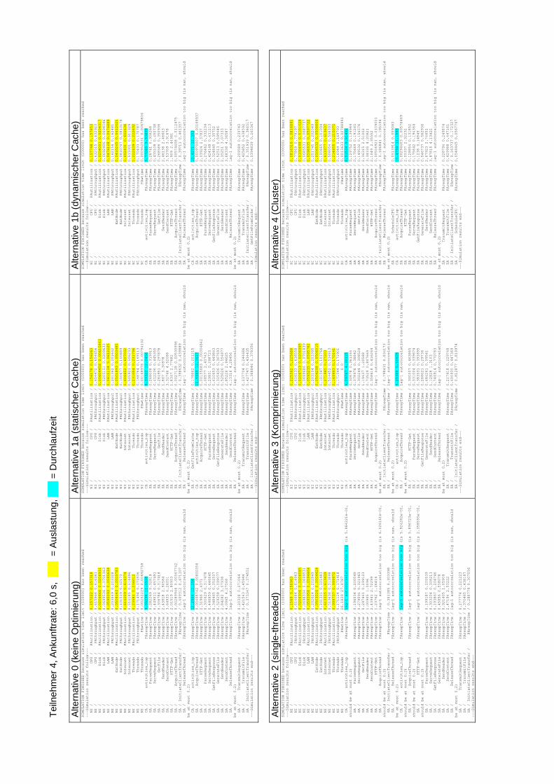
Teiln
ehm
er 4
, Ank
unftr
ate:
6,0
s,
___
= A
usla
stun
g, _
__ =
Dur
chla
ufze
it A
ltern
ativ
e 0
(kei
ne O
ptim
ieru
ng)
Alte
rnat
ive
1a (s
tatis
cher
Cac
he)
Alte
rnat
ive
1b (d
ynam
isch
er C
ache
) SIMULATION FINISHED because simulation time limit (100000) has been reached
---Simulation results follow---
NI / CPU / PAutilization / 0.157222 0.157318
NI / CPU / PAthroughput / 0.615966 0.616361
NI / Disk / PAutilization / 0.0206666 0.0206931
NI / Disk / PAthroughput / 0.0699536 0.0701363
NI / LAN / PAutilization / 0.0595093 0.0595634
NI / LAN / PAthroughput / 0.203049 0.203328
NI / ExtNode / PAutilization / 0.0504143 0.0505783
NI / ExtNode / PAthroughput / 0.101519 0.10173
NI / Internet / PAutilization / 0.614209 0.614374
NI / Internet / PAthroughput / 0.514185 0.514496
NI / Threads / PAutilization / 0.23581 0.236012
NI / Threads / PAthroughput / 0.171494 0.171836
NI / Threads / PAwtime / 0.00202229 0.00692758
CA / activities_top / PArespTime / 9.55298 11.5558
SA / ParseRequest / PArespTime / 0.282269 0.32819
SA / ServeRequest / PArespTime / 0.449011 0.457491
SA / GetFile / PArespTime / 0.306784 0.317418
SA / SendHeader / PArespTime / 2.43818 2.90584
SA / SendContent / PArespTime / 3.64933 4.26051
SA / HTTP-Get / PArespTime / 2.01519 2.80953
SA / AcquireThread / PArespTime / 0.00289946 0.00567742
SA / InitiateClientTransfer / PArespTime / 0.409312 0.471107
SA / ReleaseThread / PArespTime / lag-1 autocorrelation too big (is nan, should
be at most 0.2)
CA / activities_top / PArespTime / 12.2504 12.258
SA / AcquireThread / PArespTime / 0.00408742 0.00800356
SA / HTTP-Get / PArespTime / 2.31966 2.4371
SA / ParseRequest / PArespTime / 0.300629 0.317478
SA / ServeRequest / PArespTime / 0.446859 0.448645
SA / GetFileResponse / PArespTime / 0.348465 0.351557
SA / GenerateFile / PArespTime / 0.529258 0.599077
SA / SendHeader / PArespTime / 2.84282 3.07938
SA / SendContent / PArespTime / 4.0965 4.27568
SA / ReleaseThread / PArespTime / lag-1 autocorrelation too big (is nan, should
be at most 0.2)
SA / TransmitRequest / PArespTime / 0.20328 0.271064
SA / TransmitFile / PArespTime / 0.421543 0.45944
SA / InitiateClientTransfer / PArespTime / 0.373347 0.374551
---Simulation results end---
SIMULATION FINISHED because simulation time limit (100000) has been reached
---Simulation results follow---
NI / CPU / PAutilization / 0.156178 0.156263
NI / CPU / PAthroughput / 0.654472 0.654856
NI / Disk / PAutilization / 0.00604458 0.00615863
NI / Disk / PAthroughput / 0.0205151 0.0209633
NI / LAN / PAutilization / 0.0611134 0.0612225
NI / LAN / PAthroughput / 0.201362 0.201642
NI / ExtNode / PAutilization / 0.0501893 0.0503485
NI / ExtNode / PAthroughput / 0.100677 0.100889
NI / Internet / PAutilization / 0.606652 0.607032
NI / Internet / PAthroughput / 0.505923 0.506233
NI / Threads / PAutilization / 0.231054 0.231796
NI / Threads / PAthroughput / 0.168764 0.169113
NI / Threads / PAwtime / 0.00168978 0.00794132
CA / activities_top / PArespTime / 8.33322 12.0456
SA / ParseRequest / PArespTime / 0.288008 0.319913
SA / ServeRequest / PArespTime / 0.412236 0.445355
SA / GetFile / PArespTime / 0.284951 0.297878
SA / SendHeader / PArespTime / 1.867 3.30978
SA / SendContent / PArespTime / 3.31746 4.52088
SA / HTTP-Get / PArespTime / 1.8347 2.77682
SA / AcquireThread / PArespTime / 0.0027118 0.00530996
SA / InitiateClientTransfer / PArespTime / 0.398632 0.439889
SA / ReleaseThread / PArespTime / lag-1 autocorrelation too big (is nan, should
be at most 0.2)
SA / GetFileFromCache / PArespTime / 0.178862 0.201215
CA / activities_top / PArespTime / 11.6949 12.3617
SA / AcquireThread / PArespTime / 0.00155683 0.00304842
SA / HTTP-Get / PArespTime / 2.08577 2.43743
SA / ParseRequest / PArespTime / 0.29851 0.298723
SA / ServeRequest / PArespTime / 0.410653 0.449843
SA / GetFileResponse / PArespTime / 0.315436 0.367693
SA / GenerateFile / PArespTime / 0.525026 0.554877
SA / SendHeader / PArespTime / 2.85226 2.94625
SA / SendContent / PArespTime / 4.13316 4.28456
SA / ReleaseThread / PArespTime / lag-1 autocorrelation too big (is nan, should
be at most 0.2)
SA / TransmitRequest / PArespTime / 0.237704 0.244686
SA / TransmitFile / PArespTime / 0.427747 0.434435
SA / InitiateClientTransfer / PArespTime / 0.368846 0.378356
---Simulation results end---
SIMULATION FINISHED because simulation time limit (100000) has been reached
---Simulation results follow---
NI / CPU / PAutilization / 0.157748 0.157853
NI / CPU / PAthroughput / 0.632515 0.632923
NI / Disk / PAutilization / 0.0204001 0.0204317
NI / Disk / PAthroughput / 0.0692406 0.0694546
NI / LAN / PAutilization / 0.0476128 0.0476889
NI / LAN / PAthroughput / 0.162158 0.162481
NI / ExtNode / PAutilization / 0.0410245 0.0412021
NI / ExtNode / PAthroughput / 0.0810707 0.0813179
NI / Internet / PAutilization / 0.602431 0.602636
NI / Internet / PAthroughput / 0.511001 0.511329
NI / Threads / PAutilization / 0.222439 0.222692
NI / Threads / PAthroughput / 0.170433 0.170787
NI / Threads / PAwtime / 0.000952531 0.00679856
CA / activities_top / PArespTime / 9.77045 9.93899
SA / ParseRequest / PArespTime / 0.28741 0.308268
SA / ServeRequest / PArespTime / 0.435108 0.450738
SA / GetFile / PArespTime / 0.268586 0.350936
SA / SendHeader / PArespTime / 2.46138 2.46603
SA / SendContent / PArespTime / 3.53709 3.91678
SA / HTTP-Get / PArespTime / 1.909 2.44381
SA / AcquireThread / PArespTime / 0.00574408 0.0112475
SA / InitiateClientTransfer / PArespTime / 0.39711 0.461357
SA / ReleaseThread / PArespTime / lag-1 autocorrelation too big (is nan, should
be at most 0.2)
CA / activities_top / PArespTime / 10.4271 12.353
SA / AcquireThread / PArespTime / 0.000970007 0.00189937
SA / HTTP-Get / PArespTime / 2.03924 2.37837
SA / ParseRequest / PArespTime / 0.276462 0.332234
SA / ServeRequest / PArespTime / 0.424148 0.431213
SA / GetFileResponse / PArespTime / 0.324845 0.35752
SA / GenerateFile / PArespTime / 0.52513 0.595446
SA / SendHeader / PArespTime / 2.35251 3.07333
SA / SendContent / PArespTime / 3.68338 4.36587
SA / ReleaseThread / PArespTime / lag-1 autocorrelation too big (is nan, should
be at most 0.2)
SA / TransmitRequest / PArespTime / 0.209589 0.239743
SA / TransmitFile / PArespTime / 0.425852 0.438592
SA / InitiateClientTransfer / PArespTime / 0.351919 0.386517
SA / GetFileFromCache / PArespTime / 0.0394839 0.265367
---Simulation results end---
Alte
rnat
ive
2 (s
ingl
e-th
read
ed)
Alte
rnat
ive
3 (K
ompr
imie
rung
) A
ltern
ativ
e 4
(Clu
ster
) SIMULATION FINISHED because simulation time limit (100000) has been reached
---Simulation results follow---
NI / CPU / PAutilization / 0.1569 0.156963
NI / CPU / PAthroughput / 0.614684 0.614963
NI / Disk / PAutilization / 0.0206306 0.0206585
NI / Disk / PAthroughput / 0.0698334 0.0699531
NI / LAN / PAutilization / 0.0593958 0.0594464
NI / LAN / PAthroughput / 0.202624 0.202849
NI / ExtNode / PAutilization / 0.0503026 0.0504424
NI / ExtNode / PAthroughput / 0.101311 0.101483
NI / Internet / PAutilization / 0.613315 0.613439
NI / Internet / PAthroughput / 0.513638 0.513898
NI / Threads / PAutilization / 0.999737 0.999972
NI / Threads / PAthroughput / 0.171124 0.171418
NI / Threads / PAwtime / 26.1839 27.0787
CA / activities_top / PArespTime / lag-1 autocorrelation too big (is 5.984221e-01,
should be at most 0.2)
SA / ParseRequest / PArespTime / 0.196034 0.200549
SA / ServeRequest / PArespTime / 0.279591 0.321963
SA / GetFile / PArespTime / 0.297441 0.299123
SA / SendHeader / PArespTime / 1.00905 1.0096
SA / SendContent / PArespTime / 2.43941 2.72299
SA / HTTP-Get / PArespTime / 1.23762 1.46416
SA / AcquireThread / PArespTime / lag-1 autocorrelation too big (is 6.026161e-01,
should be at most 0.2)
SA / InitiateClientTransfer / PArespTime / 0.301385 0.303398
SA / ReleaseThread / PArespTime / lag-1 autocorrelation too big (is nan, should
be at most 0.2)
CA / activities_top / PArespTime / lag-1 autocorrelation too big (is 5.924282e-01,
should be at most 0.2)
SA / AcquireThread / PArespTime / lag-1 autocorrelation too big (is 5.896723e-01,
should be at most 0.2)
SA / HTTP-Get / PArespTime / lag-1 autocorrelation too big (is 2.358595e-01,
should be at most 0.2)
SA / ParseRequest / PArespTime / 0.199187 0.205539
SA / ServeRequest / PArespTime / 0.303204 0.308211
SA / GetFileResponse / PArespTime / 0.193867 0.204746
SA / GenerateFile / PArespTime / 0.45856 0.558078
SA / SendHeader / PArespTime / 0.921405 1.05909
SA / SendContent / PArespTime / 2.47194 2.53222
SA / ReleaseThread / PArespTime / lag-1 autocorrelation too big (is nan, should
be at most 0.2)
SA / TransmitRequest / PArespTime / 0.177774 0.221223
SA / TransmitFile / PArespTime / 0.370465 0.438187
SA / InitiateClientTransfer / PArespTime / 0.288779 0.307056
---Simulation results end---
SIMULATION FINISHED because simulation time limit (100000) has been reached
---Simulation results follow---
NI / CPU / PAutilization / 0.225562 0.225686
NI / CPU / PAthroughput / 0.616133 0.616558
NI / Disk / PAutilization / 0.0206713 0.0206995
NI / Disk / PAthroughput / 0.0699686 0.0701839
NI / LAN / PAutilization / 0.0595235 0.0595782
NI / LAN / PAthroughput / 0.203104 0.203395
NI / ExtNode / PAutilization / 0.0504298 0.0506015
NI / ExtNode / PAthroughput / 0.101547 0.101766
NI / Internet / PAutilization / 0.271945 0.27203
NI / Internet / PAthroughput / 0.514452 0.514813
NI / Threads / PAutilization / 0.169993 0.170141
NI / Threads / PAthroughput / 0.171544 0.171901
NI / Threads / PAwtime / 0 0
CA / activities_top / PArespTime / 4.09767 4.30115
SA / ParseRequest / PArespTime / 0.30878 0.361164
SA / ServeRequest / PArespTime / 0.378978 0.38842
SA / GetFile / PArespTime / 0.302244 0.308528
SA / SendHeader / PArespTime / 1.19437 1.20588
SA / SendContent / PArespTime / 0.73529 0.807669
SA / HTTP-Get / PArespTime / 0.358618 0.416264
SA / AcquireThread / PArespTime / lag-1 autocorrelation too big (is nan, should
be at most 0.2)
SA / InitiateClientTransfer / PArespTime / 0.798431 0.834173
SA / ReleaseThread / PArespTime / lag-1 autocorrelation too big (is nan, should
be at most 0.2)
CA / activities_top / PArespTime / 5.25388 5.50625
SA / AcquireThread / PArespTime / lag-1 autocorrelation too big (is nan, should
be at most 0.2)
SA / HTTP-Get / PArespTime / 0.300507 0.463865
SA / ParseRequest / PArespTime / 0.331004 0.339674
SA / ServeRequest / PArespTime / 0.383531 0.391895
SA / GetFileResponse / PArespTime / 0.288021 0.29736
SA / GenerateFile / PArespTime / 0.484261 0.59541
SA / SendHeader / PArespTime / 1.12828 1.3103
SA / SendContent / PArespTime / 0.746914 0.770783
SA / ReleaseThread / PArespTime / lag-1 autocorrelation too big (is nan, should
be at most 0.2)
SA / TransmitRequest / PArespTime / 0.217418 0.229748
SA / TransmitFile / PArespTime / 0.400935 0.447369
SA / InitiateClientTransfer / PArespTime / 0.812877 0.819974
---Simulation results end---
SIMULATION FINISHED because simulation time limit (100000) has been reached
---Simulation results follow---
NI / CPU / PAutilization / 0.0816316 0.0816891
NI / CPU / PAthroughput / 0.77869 0.779197
NI / Disk / PAutilization / 0.0100698 0.0101029
NI / Disk / PAthroughput / 0.0685531 0.0687737
NI / LAN / PAutilization / 0.0596935 0.0597722
NI / LAN / PAthroughput / 0.201745 0.202049
NI / ExtNode / PAutilization / 0.0506532 0.0508806
NI / ExtNode / PAthroughput / 0.100865 0.101094
NI / Internet / PAutilization / 0.613377 0.613637
NI / Internet / PAthroughput / 0.508054 0.508393
NI / Threads / PAutilization / 0.214855 0.215075
NI / Threads / PAthroughput / 0.16944 0.169793
NI / Threads / PAwtime / 0.0013633 0.00788991
CA / activities_top / PArespTime / 8.51534 9.81492
SA / ParseRequest / PArespTime / 0.129752 0.134944
SA / ServeRequest / PArespTime / 0.175669 0.191265
SA / GetFile / PArespTime / 0.149532 0.154576
SA / SendHeader / PArespTime / 2.36315 2.51002
SA / SendContent / PArespTime / 3.34335 4.20821
SA / HTTP-Get / PArespTime / 2.1049 2.35552
SA / AcquireThread / PArespTime / 0.00556921 0.0109051
SA / InitiateClientTransfer / PArespTime / 0.186841 0.195594
SA / ReleaseThread / PArespTime / lag-1 autocorrelation too big (is nan, should
be at most 0.2)
SA / ScheduleCPU / PArespTime / 0.0513914 0.059083
CA / activities_top / PArespTime / 10.4794 11.1593
SA / AcquireThread / PArespTime / 0.00294403 0.00576469
SA / HTTP-Get / PArespTime / 2.05337 2.32232
SA / ParseRequest / PArespTime / 0.128854 0.131852
SA / ServeRequest / PArespTime / 0.175642 0.194364
SA / GetFileResponse / PArespTime / 0.1238 0.14849
SA / GenerateFile / PArespTime / 0.546737 0.562936
SA / SendHeader / PArespTime / 2.67923 2.74651
SA / SendContent / PArespTime / 3.87816 4.13422
SA / ReleaseThread / PArespTime / lag-1 autocorrelation too big (is nan, should
be at most 0.2)
SA / TransmitRequest / PArespTime / 0.228794 0.249874
SA / TransmitFile / PArespTime / 0.429988 0.447161
SA / InitiateClientTransfer / PArespTime / 0.163737 0.172327
SA / ScheduleCPU / PArespTime / 0.0548445 0.0567767
---Simulation results end---
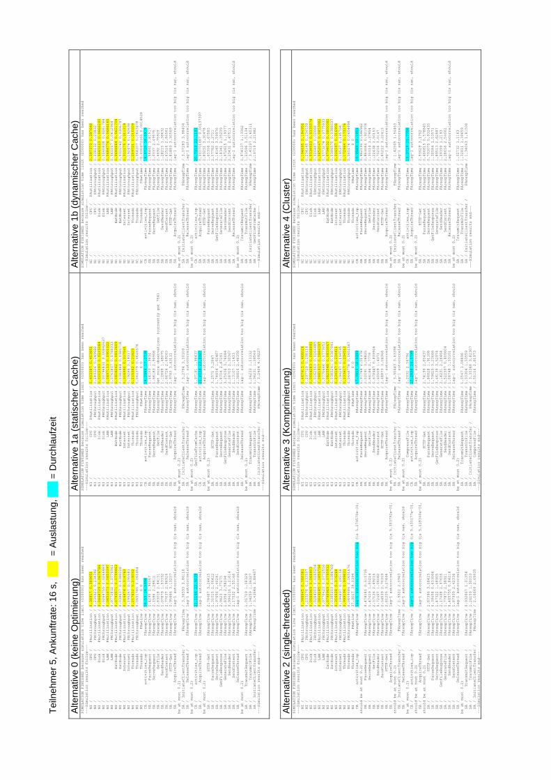
Teiln
ehm
er 5
, Ank
unftr
ate:
16
s, _
__ =
Aus
last
ung,
___
= D
urch
lauf
zeit
Alte
rnat
ive
0 (k
eine
Opt
imie
rung
) A
ltern
ativ
e 1a
(sta
tisch
er C
ache
) A
ltern
ativ
e 1b
(dyn
amis
cher
Cac
he)
SIMULATION FINISHED because simulation time limit (100000) has been reached
---Simulation results follow---
NI / CPU / PAutilization / 0.38917 0.389651
NI / CPU / PAthroughput / 0.234023 0.234392
NI / Disk / PAutilization / 0.0668729 0.0670786
NI / Disk / PAthroughput / 0.0264755 0.0266489
NI / LAN / PAutilization / 0.0851673 0.0853397
NI / LAN / PAthroughput / 0.0772832 0.0775361
NI / ExtNode / PAutilization / 0.0793571 0.0799463
NI / ExtNode / PAthroughput / 0.038637 0.0388228
NI / Internet / PAutilization / 0.316474 0.316763
NI / Internet / PAthroughput / 0.195267 0.195581
NI / Threads / PAutilization / 0.217612 0.218052
NI / Threads / PAthroughput / 0.0651785 0.065454
NI / Threads / PAwtime / 0 0
CA / activities_top / PArespTime / 16.59 18.5996
SA / ParseRequest / PArespTime / 1.4295 1.94567
SA / ServeRequest / PArespTime / 2.1586 2.29612
SA / GetFile / PArespTime / 2.83018 2.84151
SA / SendHeader / PArespTime / 1.07879 1.53332
SA / SendContent / PArespTime / 2.77037 2.96926
SA / HTTP-Get / PArespTime / 2.95666 3.15257
SA / AcquireThread / PArespTime / lag-1 autocorrelation too big (is nan, should
be at most 0.2)
SA / InitiateClientTransfer / PArespTime / 3.36593 3.86116
SA / ReleaseThread / PArespTime / lag-1 autocorrelation too big (is nan, should
be at most 0.2)
CA / activities_top / PArespTime / 21.1166 22.9039
SA / AcquireThread / PArespTime / lag-1 autocorrelation too big (is nan, should
be at most 0.2)
SA / HTTP-Get / PArespTime / 2.78467 3.24415
SA / ParseRequest / PArespTime / 1.31015 2.06422
SA / ServeRequest / PArespTime / 1.97656 2.40241
SA / GetFileResponse / PArespTime / 2.9823 3.77275
SA / GenerateFile / PArespTime / 1.8356 2.58294
SA / SendHeader / PArespTime / 0.994216 1.21614
SA / SendContent / PArespTime / 2.17532 2.55168
SA / ReleaseThread / PArespTime / lag-1 autocorrelation too big (is nan, should
be at most 0.2)
SA / TransmitRequest / PArespTime / 1.01719 1.08329
SA / TransmitFile / PArespTime / 1.34259 1.36327
SA / InitiateClientTransfer / PArespTime / 3.43646 3.88457
---Simulation results end---
SIMULATION FINISHED because simulation time limit (100000) has been reached
---Simulation results follow---
NI / CPU / PAutilization / 0.403387 0.403851
NI / CPU / PAthroughput / 0.249326 0.249682
NI / Disk / PAutilization / 0.0205093 0.0215084
NI / Disk / PAthroughput / 0.00796831 0.00842637
NI / LAN / PAutilization / 0.0897153 0.0901022
NI / LAN / PAthroughput / 0.0765837 0.0768333
NI / ExtNode / PAutilization / 0.0808262 0.0813609
NI / ExtNode / PAthroughput / 0.0382884 0.0384718
NI / Internet / PAutilization / 0.316992 0.317541
NI / Internet / PAthroughput / 0.19285 0.19317
NI / Threads / PAutilization / 0.215562 0.21623
NI / Threads / PAthroughput / 0.064379 0.0646576
NI / Threads / PAwtime / 0 0
CA / activities_top / PArespTime / 16.2966 17.2738
SA / ParseRequest / PArespTime / 1.44103 1.9834
SA / ServeRequest / PArespTime / 1.68183 2.90908
SA / GetFile / PArespTime / Get more observations (currently got 754)
SA / SendHeader / PArespTime / 1.12869 1.49075
SA / SendContent / PArespTime / 2.66724 2.69263
SA / HTTP-Get / PArespTime / 2.9783 3.43111
SA / AcquireThread / PArespTime / lag-1 autocorrelation too big (is nan, should
be at most 0.2)
SA / InitiateClientTransfer / PArespTime / 3.2794 3.50109
SA / ReleaseThread / PArespTime / lag-1 autocorrelation too big (is nan, should
be at most 0.2)
SA / GetFileFromCache / PArespTime / 1.97181 1.98437
CA / activities_top / PArespTime / 21.4039 23.8967
SA / AcquireThread / PArespTime / lag-1 autocorrelation too big (is nan, should
be at most 0.2)
SA / HTTP-Get / PArespTime / 3.2571 3.2847
SA / ParseRequest / PArespTime / 1.74854 1.82467
SA / ServeRequest / PArespTime / 1.8704 2.47291
SA / GetFileResponse / PArespTime / 3.25656 3.76684
SA / GenerateFile / PArespTime / 2.08703 2.30367
SA / SendHeader / PArespTime / 1.13107 1.1433
SA / SendContent / PArespTime / 2.38816 2.46158
SA / ReleaseThread / PArespTime / lag-1 autocorrelation too big (is nan, should
be at most 0.2)
SA / TransmitRequest / PArespTime / 1.06233 1.15132
SA / TransmitFile / PArespTime / 1.36231 1.39549
SA / InitiateClientTransfer / PArespTime / 3.2404 4.09227
---Simulation results end---
SIMULATION FINISHED because simulation time limit (200000) has been reached
---Simulation results follow---
NI / CPU / PAutilization / 0.397373 0.397648
NI / CPU / PAthroughput / 0.238132 0.23832
NI / Disk / PAutilization / 0.0665123 0.0666295
NI / Disk / PAthroughput / 0.0260838 0.0261784
NI / LAN / PAutilization / 0.0684776 0.0686165
NI / LAN / PAthroughput / 0.061157 0.0612964
NI / ExtNode / PAutilization / 0.0648864 0.0651704
NI / ExtNode / PAthroughput / 0.0305762 0.0306797
NI / Internet / PAutilization / 0.311175 0.311319
NI / Internet / PAthroughput / 0.192476 0.192638
NI / Threads / PAutilization / 0.209721 0.210009
NI / Threads / PAthroughput / 0.064207 0.0643478
NI / Threads / PAwtime / -0.000471165 0.0014528
CA / activities_top / PArespTime / 16.0725 18.5919
SA / ParseRequest / PArespTime / 1.58461 1.81517
SA / ServeRequest / PArespTime / 2.0337 2.49575
SA / GetFile / PArespTime / 2.6692 2.75929
SA / SendHeader / PArespTime / 1.28215 1.38632
SA / SendContent / PArespTime / 2.61516 2.84561
SA / HTTP-Get / PArespTime / 2.81483 3.30569
SA / AcquireThread / PArespTime / lag-1 autocorrelation too big (is nan, should
be at most 0.2)
SA / InitiateClientTransfer / PArespTime / 3.07283 3.98404
SA / ReleaseThread / PArespTime / lag-1 autocorrelation too big (is nan, should
be at most 0.2)
CA / activities_top / PArespTime / 20.7919 22.1191
SA / AcquireThread / PArespTime / 0.000701687 0.00137397
SA / HTTP-Get / PArespTime / 2.89251 3.30478
SA / ParseRequest / PArespTime / 1.65358 1.67585
SA / ServeRequest / PArespTime / 2.07782 2.2721
SA / GetFileResponse / PArespTime / 3.14145 3.59976
SA / GenerateFile / PArespTime / 2.18341 2.35239
SA / SendHeader / PArespTime / 0.972615 1.19377
SA / SendContent / PArespTime / 2.23431 2.47511
SA / ReleaseThread / PArespTime / lag-1 autocorrelation too big (is nan, should
be at most 0.2)
SA / TransmitRequest / PArespTime / 0.974537 1.13362
SA / TransmitFile / PArespTime / 1.21596 1.51134
SA / InitiateClientTransfer / PArespTime / 3.41237 3.65311
SA / GetFileFromCache / PArespTime / 2.19719 2.21982
---Simulation results end---
Alte
rnat
ive
2 (s
ingl
e-th
read
ed)
Alte
rnat
ive
3 (K
ompr
imie
rung
) A
ltern
ativ
e 4
(Clu
ster
) SIMULATION FINISHED because simulation time limit (100000) has been reached
---Simulation results follow---
NI / CPU / PAutilization / 0.388045 0.388381
NI / CPU / PAthroughput / 0.233278 0.233557
NI / Disk / PAutilization / 0.0666969 0.066903
NI / Disk / PAthroughput / 0.0264103 0.0265254
NI / LAN / PAutilization / 0.0849245 0.0850794
NI / LAN / PAthroughput / 0.0770423 0.0772556
NI / ExtNode / PAutilization / 0.0790969 0.0795912
NI / ExtNode / PAthroughput / 0.0385203 0.0386769
NI / Internet / PAutilization / 0.316028 0.316268
NI / Internet / PAthroughput / 0.194897 0.195158
NI / Threads / PAutilization / 0.999196 0.999831
NI / Threads / PAthroughput / 0.0649484 0.0651676
NI / Threads / PAwtime / 37.3017 39.3394
CA / activities_top / PArespTime / lag-1 autocorrelation too big (is 5.279570e-01,
should be at most 0.2)
SA / ParseRequest / PArespTime / 0.478181 0.511735
SA / ServeRequest / PArespTime / 1.47419 1.55214
SA / GetFile / PArespTime / 2.57126 2.69216
SA / SendHeader / PArespTime / 0.72457 1.06082
SA / SendContent / PArespTime / 2.54539 2.70359
SA / HTTP-Get / PArespTime / 2.81225 3.27446
SA / AcquireThread / PArespTime / lag-1 autocorrelation too big (is 5.353792e-01,
should be at most 0.2)
SA / InitiateClientTransfer / PArespTime / 2.5322 2.5943
SA / ReleaseThread / PArespTime / lag-1 autocorrelation too big (is nan, should
be at most 0.2)
CA / activities_top / PArespTime / lag-1 autocorrelation too big (is 5.430177e-01,
should be at most 0.2)
SA / AcquireThread / PArespTime / lag-1 autocorrelation too big (is 5.418340e-01,
should be at most 0.2)
SA / HTTP-Get / PArespTime / 2.87396 3.08415
SA / ParseRequest / PArespTime / 0.39458 0.633086
SA / ServeRequest / PArespTime / 1.47322 1.48905
SA / GetFileResponse / PArespTime / 2.17408 2.97656
SA / GenerateFile / PArespTime / 1.77873 2.38911
SA / SendHeader / PArespTime / 0.465755 0.84216
SA / SendContent / PArespTime / 1.87939 2.42336
SA / ReleaseThread / PArespTime / lag-1 autocorrelation too big (is nan, should
be at most 0.2)
SA / TransmitRequest / PArespTime / 0.932667 1.01356
SA / TransmitFile / PArespTime / 1.26159 1.30053
SA / InitiateClientTransfer / PArespTime / 2.16669 2.69935
---Simulation results end---
SIMULATION FINISHED because simulation time limit (100000) has been reached
---Simulation results follow---
NI / CPU / PAutilization / 0.467415 0.468026
NI / CPU / PAthroughput / 0.297729 0.298118
NI / Disk / PAutilization / 0.0664283 0.0668891
NI / Disk / PAthroughput / 0.0262569 0.0264485
NI / LAN / PAutilization / 0.0881917 0.0884397
NI / LAN / PAthroughput / 0.0770666 0.0773051
NI / ExtNode / PAutilization / 0.0825548 0.0833067
NI / ExtNode / PAthroughput / 0.0385291 0.0387041
NI / Internet / PAutilization / 0.234147 0.234411
NI / Internet / PAthroughput / 0.194297 0.194595
NI / Threads / PAutilization / 0.233617 0.234512
NI / Threads / PAthroughput / 0.0648778 0.0651567
NI / Threads / PAwtime / 0 0
CA / activities_top / PArespTime / 17.3815 18.9393
SA / ParseRequest / PArespTime / 1.97764 2.01178
SA / ServeRequest / PArespTime / 2.02091 3.06825
SA / GetFile / PArespTime / 2.66186 2.7779
SA / SendHeader / PArespTime / 0.678447 0.839946
SA / SendContent / PArespTime / 1.40509 1.4371
SA / HTTP-Get / PArespTime / 2.48873 3.04366
SA / AcquireThread / PArespTime / lag-1 autocorrelation too big (is nan, should
be at most 0.2)
SA / InitiateClientTransfer / PArespTime / 3.50443 3.63396
SA / ReleaseThread / PArespTime / lag-1 autocorrelation too big (is nan, should
be at most 0.2)
SA / CompressFile / PArespTime / 2.2032 2.56794
CA / activities_top / PArespTime / 22.2858 24.5799
SA / AcquireThread / PArespTime / lag-1 autocorrelation too big (is nan, should
be at most 0.2)
SA / HTTP-Get / PArespTime / 2.74199 2.85437
SA / ParseRequest / PArespTime / 1.86828 1.91108
SA / ServeRequest / PArespTime / 1.79615 3.23668
SA / GetFileResponse / PArespTime / 3.46139 3.52974
SA / GenerateFile / PArespTime / 2.14231 2.26464
SA / SendHeader / PArespTime / 0.522397 0.800604
SA / SendContent / PArespTime / 1.08748 1.33101
SA / ReleaseThread / PArespTime / lag-1 autocorrelation too big (is nan, should
be at most 0.2)
SA / TransmitRequest / PArespTime / 1.0547 1.08696
SA / TransmitFile / PArespTime / 1.33304 1.33559
SA / InitiateClientTransfer / PArespTime / 3.35388 3.82307
SA / CompressFile / PArespTime / 2.51116 2.81973
---Simulation results end---
SIMULATION FINISHED because simulation time limit (100000) has been reached
---Simulation results follow---
NI / CPU / PAutilization / 0.194695 0.194956
NI / CPU / PAthroughput / 0.234145 0.234539
NI / Disk / PAutilization / 0.0334503 0.0335574
NI / Disk / PAthroughput / 0.026487 0.02668
NI / LAN / PAutilization / 0.0852047 0.0853982
NI / LAN / PAthroughput / 0.0773274 0.0775933
NI / ExtNode / PAutilization / 0.0794032 0.0800381
NI / ExtNode / PAthroughput / 0.0386575 0.0388537
NI / Internet / PAutilization / 0.316597 0.316908
NI / Internet / PAthroughput / 0.19537 0.195704
NI / Threads / PAutilization / 0.172964 0.173176
NI / Threads / PAthroughput / 0.065176 0.0654494
NI / Threads / PAwtime / 0 0
CA / activities_top / PArespTime / 10.9589 12.1051
SA / ParseRequest / PArespTime / 0.462194 0.546962
SA / ServeRequest / PArespTime / 0.863064 0.921978
SA / GetFile / PArespTime / 1.35114 1.37954
SA / SendHeader / PArespTime / 1.22438 1.50153
SA / SendContent / PArespTime / 2.75256 3.0147
SA / HTTP-Get / PArespTime / 2.85212 3.22413
SA / AcquireThread / PArespTime / lag-1 autocorrelation too big (is nan, should
be at most 0.2)
SA / InitiateClientTransfer / PArespTime / 1.42505 1.54463
SA / ReleaseThread / PArespTime / lag-1 autocorrelation too big (is nan, should
be at most 0.2)
CA / activities_top / PArespTime / 15.3719 15.7756
SA / AcquireThread / PArespTime / lag-1 autocorrelation too big (is nan, should
be at most 0.2)
SA / HTTP-Get / PArespTime / 2.93629 3.1702
SA / ParseRequest / PArespTime / 0.406815 0.578845
SA / ServeRequest / PArespTime / 0.793075 0.932435
SA / GetFileResponse / PArespTime / 1.30584 1.53571
SA / GenerateFile / PArespTime / 1.89513 2.62887
SA / SendHeader / PArespTime / 1.09399 1.2193
SA / SendContent / PArespTime / 2.28658 2.54062
SA / ReleaseThread / PArespTime / lag-1 autocorrelation too big (is nan, should
be at most 0.2)
SA / TransmitRequest / PArespTime / 1.02732 1.1163
SA / TransmitFile / PArespTime / 1.32811 1.39659
SA / InitiateClientTransfer / PArespTime / 1.34043 1.61508
---Simulation results end---
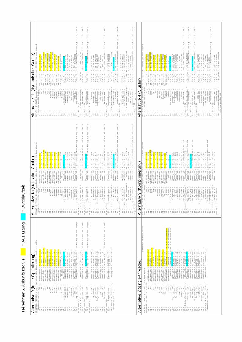
Teiln
ehm
er 6
, Ank
unftr
ate:
5 s
, __
_ =
Aus
last
ung,
___
= D
urch
lauf
zeit
Alte
rnat
ive
0 (k
eine
Opt
imie
rung
) A
ltern
ativ
e 1a
(sta
tisch
er C
ache
) A
ltern
ativ
e 1b
(dyn
amis
cher
Cac
he)
SIMULATION FINISHED because simulation time limit (100000) has been reached
---Simulation results follow---
NI / CPU / PAutilization / 0.245376 0.245507
NI / CPU / PAthroughput / 0.738005 0.738406
NI / Disk / PAutilization / 0.0495381 0.0495928
NI / Disk / PAthroughput / 0.0836587 0.0838539
NI / LAN / PAutilization / 0.119142 0.119226
NI / LAN / PAthroughput / 0.243483 0.243745
NI / ExtNode / PAutilization / 0.121259 0.121538
NI / ExtNode / PAthroughput / 0.121736 0.121927
NI / Internet / PAutilization / 0.286802 0.286882
NI / Internet / PAthroughput / 0.616118 0.616461
NI / Threads / PAutilization / 0.188267 0.188375
NI / Threads / PAthroughput / 0.20546 0.205814
NI / Threads / PAwtime / 0 0
CA / activities_top / PArespTime / 3.98577 4.13195
SA / ParseRequest / PArespTime / 0.411547 0.441909
SA / ServeRequest / PArespTime / 0.455867 0.60834
SA / GetFile / PArespTime / 0.585218 0.6821
SA / SendHeader / PArespTime / 0.51459 0.585894
SA / SendContent / PArespTime / 1.19747 1.20171
SA / HTTP-Get / PArespTime / 0.338601 0.428296
SA / AcquireThread / PArespTime / lag-1 autocorrelation too big (is nan, should
be at most 0.2)
SA / InitiateClientTransfer / PArespTime / 0.325771 0.340413
SA / ReleaseThread / PArespTime / lag-1 autocorrelation too big (is nan, should
be at most 0.2)
CA / activities_top / PArespTime / 6.36789 6.38932
SA / AcquireThread / PArespTime / lag-1 autocorrelation too big (is nan, should
be at most 0.2)
SA / HTTP-Get / PArespTime / 0.348176 0.399018
SA / ParseRequest / PArespTime / 0.397544 0.472467
SA / ServeRequest / PArespTime / 0.539708 0.547059
SA / GetFileResponse / PArespTime / 0.640599 0.646527
SA / GenerateFile / PArespTime / 1.12274 1.20887
SA / SendHeader / PArespTime / 0.574718 0.587629
SA / SendContent / PArespTime / 1.09597 1.22157
SA / ReleaseThread / PArespTime / lag-1 autocorrelation too big (is nan, should
be at most 0.2)
SA / TransmitRequest / PArespTime / 0.27381 0.299746
SA / TransmitFile / PArespTime / 0.816032 0.91436
SA / InitiateClientTransfer / PArespTime / 0.294718 0.355958
---Simulation results end---
SIMULATION FINISHED because simulation time limit (100000) has been reached
---Simulation results follow---
NI / CPU / PAutilization / 0.245042 0.24517
NI / CPU / PAthroughput / 0.735973 0.736375
NI / Disk / PAutilization / 0.0320284 0.0320742
NI / Disk / PAthroughput / 0.0819708 0.0822657
NI / LAN / PAutilization / 0.120995 0.121063
NI / LAN / PAthroughput / 0.244965 0.245192
NI / ExtNode / PAutilization / 0.122074 0.122287
NI / ExtNode / PAthroughput / 0.122483 0.122652
NI / Internet / PAutilization / 0.276434 0.276563
NI / Internet / PAthroughput / 0.613354 0.613707
NI / Threads / PAutilization / 0.185516 0.185626
NI / Threads / PAthroughput / 0.204529 0.204901
NI / Threads / PAwtime / 0 0
CA / activities_top / PArespTime / 3.78573 3.9617
SA / ParseRequest / PArespTime / 0.444721 0.467535
SA / ServeRequest / PArespTime / 0.488471 0.589405
SA / GetFile / PArespTime / 0.555654 0.684321
SA / SendHeader / PArespTime / 0.340748 0.488038
SA / SendContent / PArespTime / 1.12703 1.21341
SA / HTTP-Get / PArespTime / 0.285371 0.381355
SA / AcquireThread / PArespTime / lag-1 autocorrelation too big (is nan, should
be at most 0.2)
SA / InitiateClientTransfer / PArespTime / 0.310066 0.371303
SA / ReleaseThread / PArespTime / lag-1 autocorrelation too big (is nan, should
be at most 0.2)
CA / activities_top / PArespTime / 5.97984 6.53122
SA / AcquireThread / PArespTime / lag-1 autocorrelation too big (is nan, should
be at most 0.2)
SA / HTTP-Get / PArespTime / 0.263914 0.442044
SA / ParseRequest / PArespTime / 0.428611 0.43898
SA / ServeRequest / PArespTime / 0.538351 0.552778
SA / GetFileResponse / PArespTime / 0.608402 0.67146
SA / GenerateFile / PArespTime / 1.06646 1.17545
SA / SendHeader / PArespTime / 0.46322 0.63955
SA / SendContent / PArespTime / 1.02209 1.25803
SA / ReleaseThread / PArespTime / lag-1 autocorrelation too big (is nan, should
be at most 0.2)
SA / TransmitRequest / PArespTime / 0.261174 0.308109
SA / TransmitFile / PArespTime / 0.835488 0.88932
SA / InitiateClientTransfer / PArespTime / 0.31832 0.329313
CA / activities_top / PArespTime / 3.39333 3.59902
SA / HTTP-Get / PArespTime / 0.353033 0.372622
SA / Aquire Thread / PArespTime / lag-1 autocorrelation too big (is nan, should
be at most 0.2)
SA / Parse Request / PArespTime / 0.42406 0.427072
SA / Serve Request / PArespTime / 0.513291 0.556814
SA / Load FIle From Cache / PArespTime / 0.305654 0.33014
SA / Initiate Client Transfer / PArespTime / 0.333906 0.336704
SA / Send Header / PArespTime / 0.366435 0.459802
SA / Send Content / PArespTime / 1.04707 1.16575
SA / Release Thread / PArespTime / lag-1 autocorrelation too big (is nan, should
be at most 0.2)
---Simulation results end---
SIMULATION FINISHED because simulation time limit (100000) has been reached
---Simulation results follow---
NI / CPU / PAutilization / 0.227316 0.227439
NI / CPU / PAthroughput / 0.698756 0.699188
NI / Disk / PAutilization / 0.0550796 0.0552201
NI / Disk / PAthroughput / 0.104822 0.105129
NI / LAN / PAutilization / 0.0973758 0.097543
NI / LAN / PAthroughput / 0.192103 0.192337
NI / ExtNode / PAutilization / 0.0949433 0.0951577
NI / ExtNode / PAthroughput / 0.0960512 0.0962197
NI / Internet / PAutilization / 0.271381 0.271609
NI / Internet / PAthroughput / 0.602568 0.60296
NI / Threads / PAutilization / 0.1764 0.176561
NI / Threads / PAthroughput / 0.200932 0.201317
NI / Threads / PAwtime / 0 0
CA / activities_top / PArespTime / 3.62017 3.96434
SA / ParseRequest / PArespTime / 0.386674 0.42776
SA / ServeRequest / PArespTime / 0.483008 0.543496
SA / GetFile / PArespTime / 0.578345 0.699153
SA / SendHeader / PArespTime / 0.42546 0.428976
SA / SendContent / PArespTime / 1.03096 1.2377
SA / HTTP-Get / PArespTime / 0.297448 0.416991
SA / AcquireThread / PArespTime / lag-1 autocorrelation too big (is nan, should
be at most 0.2)
SA / InitiateClientTransfer / PArespTime / 0.313184 0.315346
SA / ReleaseThread / PArespTime / lag-1 autocorrelation too big (is nan, should
be at most 0.2)
CA / activities_top / PArespTime / 5.94575 6.32984
SA / AcquireThread / PArespTime / lag-1 autocorrelation too big (is nan, should
be at most 0.2)
SA / HTTP-Get / PArespTime / 0.310439 0.38875
SA / ParseRequest / PArespTime / 0.378186 0.434495
SA / ServeRequest / PArespTime / 0.452791 0.578686
SA / GetFileResponse / PArespTime / 0.553468 0.664517
SA / GenerateFile / PArespTime / 1.0445 1.18432
SA / SendHeader / PArespTime / 0.550142 0.58074
SA / SendContent / PArespTime / 1.11664 1.17713
SA / ReleaseThread / PArespTime / lag-1 autocorrelation too big (is nan, should
be at most 0.2)
SA / TransmitRequest / PArespTime / 0.249878 0.301986
SA / TransmitFile / PArespTime / 0.767988 0.935779
SA / InitiateClientTransfer / PArespTime / 0.301573 0.303588
CA / activities_top / PArespTime / 3.3633 3.57486
SA / HTTP-Get / PArespTime / 0.298352 0.439559
SA / Aquire Thread / PArespTime / lag-1 autocorrelation too big (is nan, should
be at most 0.2)
SA / Parse Request / PArespTime / 0.351545 0.450045
SA / Serve Request / PArespTime / 0.495101 0.518352
SA / Load From Cache / PArespTime / 0.319682 0.331638
SA / Initiate Client Transfer / PArespTime / 0.322752 0.34254
SA / Send Header / PArespTime / 0.375994 0.438909
SA / Send Content / PArespTime / 1.03888 1.21481
SA / Release Thread / PArespTime / lag-1 autocorrelation too big (is nan, should
be at most 0.2)
---Simulation results end---
Alte
rnat
ive
2 (s
ingl
e-th
read
ed)
Alte
rnat
ive
3 (K
ompr
imie
rung
) A
ltern
ativ
e 4
(Clu
ster
)
SIMULATION FINISHED because
simulation time limit (100000) has been reached
---Simulation results follow---
NI / CPU / PAutilization / 0.240858 0.240982
NI / CPU / PAthroughput / 0.728646 0.729066
NI / Disk / PAutilization / 0.0478526 0.0480071
NI / Disk / PAthroughput / 0.0817392 0.0819294
NI / LAN / PAutilization / 0.123079 0.123278
NI / LAN / PAthroughput / 0.241665 0.241943
NI / ExtNode / PAutilization / 0.121244 0.121423
NI / ExtNode / PAthroughput / 0.120831 0.121048
NI / Internet / PAutilization / 0.281857 0.282012
NI / Internet / PAthroughput / 0.607648 0.608004
NI / Threads / PAutilization / Computing the mean with no observations
NI / Threads / PAthroughput / Computing the mean with no observations
NI / Threads / PAwtime / Computing the mean with no observations
CA / activities_top / PArespTime / 3.81172 4.07612
SA / ParseRequest / PArespTime / 0.419042 0.439883
SA / ServeRequest / PArespTime / 0.523246 0.542734
SA / GetFile / PArespTime / 0.591306 0.669633
SA / SendHeader / PArespTime / 0.467062 0.563222
SA / SendContent / PArespTime / 1.05224 1.24144
SA / HTTP-Get / PArespTime / 0.290715 0.417956
SA / InitiateClientTransfer / PArespTime / 0.319909 0.349456
CA / activities_top / PArespTime / 6.08735 6.48724
SA / HTTP-Get / PArespTime / 0.318858 0.421201
SA / ParseRequest / PArespTime / 0.370522 0.483134
SA / ServeRequest / PArespTime / 0.510473 0.550982
SA / GetFileResponse / PArespTime / 0.551733 0.735234
SA / GenerateFile / PArespTime / 1.10755 1.21415
SA / SendHeader / PArespTime / 0.554285 0.554386
SA / SendContent / PArespTime / 1.1292 1.14581
SA / TransmitRequest / PArespTime / 0.250249 0.328034
SA / TransmitFile / PArespTime / 0.82059 0.915419
SA / InitiateClientTransfer / PArespTime / 0.277053 0.335728
---Simulation results end---
SIMULATION FINISHED because simulation time limit (100000) has been reached
---Simulation results follow---
NI / CPU / PAutilization / 0.341624 0.341802
NI / CPU / PAthroughput / 0.931162 0.931631
NI / Disk / PAutilization / 0.0482001 0.0483182
NI / Disk / PAthroughput / 0.0819127 0.0821327
NI / LAN / PAutilization / 0.118541 0.118643
NI / LAN / PAthroughput / 0.241384 0.241655
NI / ExtNode / PAutilization / 0.121041 0.121434
NI / ExtNode / PAthroughput / 0.120685 0.120881
NI / Internet / PAutilization / 0.132514 0.132568
NI / Internet / PAthroughput / 0.607765 0.608137
NI / Threads / PAutilization / 0.19374 0.193911
NI / Threads / PAthroughput / 0.202684 0.203056
NI / Threads / PAwtime / 0 0
CA / activities_top / PArespTime / 3.4865 3.71375
SA / ParseRequest / PArespTime / 0.484635 0.508955
SA / ServeRequest / PArespTime / 0.526999 0.631734
SA / GetFile / PArespTime / 0.606009 0.645973
SA / SendHeader / PArespTime / 0.230256 0.269561
SA / SendContent / PArespTime / 0.39377 0.398945
SA / HTTP-Get / PArespTime / 0.131449 0.152358
SA / AcquireThread / PArespTime / lag-1 autocorrelation too big
SA / InitiateClientTransfer / PArespTime / 0.401563 0.411404
SA / ReleaseThread / PArespTime / lag-1 autocorrelation too big
SA / Compress File / PArespTime / 0.632552 0.77409
CA / activities_top / PArespTime / 5.73465 6.03948
SA / AcquireThread / PArespTime / lag-1 autocorrelation too big
SA / HTTP-Get / PArespTime / 0.129102 0.148773
SA / ParseRequest / PArespTime / 0.4378 0.546339
SA / ServeRequest / PArespTime / 0.537954 0.626741
SA / GetFileResponse / PArespTime / 0.610472 0.735333
SA / GenerateFile / PArespTime / 0.998388 1.24386
SA / SendHeader / PArespTime / 0.242332 0.243685
SA / SendContent / PArespTime / 0.385637 0.405139
SA / ReleaseThread / PArespTime / lag-1 autocorrelation too big
SA / TransmitRequest / PArespTime / 0.272639 0.310592
SA / TransmitFile / PArespTime / 0.798856 0.913437
SA / InitiateClientTransfer / PArespTime / 0.38652 0.420507
SA / Compress File / PArespTime / 0.650298 0.729715
---Simulation results end---
[
SIMULATION FINISHED because simulation time limit (100000) has been reached
---Simulation results follow---
NI / CPU / PAutilization / 0.122704 0.122777
NI / CPU / PAthroughput / 0.738103 0.738529
NI / Disk / PAutilization / 0.0247721 0.0248006
NI / Disk / PAthroughput / 0.0836693 0.0838886
NI / LAN / PAutilization / 0.119155 0.11924
NI / LAN / PAthroughput / 0.243518 0.243792
NI / ExtNode / PAutilization / 0.121276 0.121572
NI / ExtNode / PAthroughput / 0.121751 0.12195
NI / Internet / PAutilization / 0.286851 0.286939
NI / Internet / PAthroughput / 0.616198 0.616558
NI / Threads / PAutilization / 0.165062 0.16516
NI / Threads / PAthroughput / 0.205459 0.205812
NI / Threads / PAwtime / 0 0
CA / activities_top / PArespTime / 2.85686 2.91466
SA / ParseRequest / PArespTime / 0.173393 0.189161
SA / ServeRequest / PArespTime / 0.19782 0.275075
SA / GetFile / PArespTime / 0.288307 0.332626
SA / SendHeader / PArespTime / 0.472142 0.510086
SA / SendContent / PArespTime / 1.14332 1.17388
SA / HTTP-Get / PArespTime / 0.365247 0.385044
SA / AcquireThread / PArespTime / lag-1 autocorrelation too big (is nan, should
be at most 0.2)
SA / InitiateClientTransfer / PArespTime / 0.12604 0.139369
SA / ReleaseThread / PArespTime / lag-1 autocorrelation too big (is nan, should
be at most 0.2)
CA / activities_top / PArespTime / 5.15404 5.29192
SA / AcquireThread / PArespTime / lag-1 autocorrelation too big (is nan, should
be at most 0.2)
SA / HTTP-Get / PArespTime / 0.359734 0.367967
SA / ParseRequest / PArespTime / 0.173325 0.194008
SA / ServeRequest / PArespTime / 0.233055 0.244038
SA / GetFileResponse / PArespTime / 0.281258 0.289674
SA / GenerateFile / PArespTime / 1.13445 1.21964
SA / SendHeader / PArespTime / 0.560563 0.563569
SA / SendContent / PArespTime / 1.09467 1.1581
SA / ReleaseThread / PArespTime / lag-1 autocorrelation too big (is nan, should
be at most 0.2)
SA / TransmitRequest / PArespTime / 0.270097 0.30248
SA / TransmitFile / PArespTime / 0.837675 0.908992
SA / InitiateClientTransfer / PArespTime / 0.126285 0.126381
---Simulation results end---
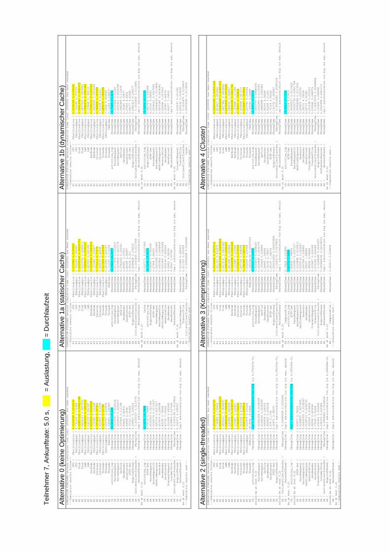
Teiln
ehm
er 7
, Ank
unftr
ate:
5.0
s,
___
= A
usla
stun
g, _
__ =
Dur
chla
ufze
it A
ltern
ativ
e 0
(kei
ne O
ptim
ieru
ng)
Alte
rnat
ive
1a (s
tatis
cher
Cac
he)
Alte
rnat
ive
1b (d
ynam
isch
er C
ache
) SIMULATION FINISHED because simulation time limit (200000) has been reached
---Simulation results follow---
NI / CPU / PAutilization / 0.0105998 0.0106033
NI / CPU / PAthroughput / 0.732248 0.732485
NI / Disk / PAutilization / 0.00821292 0.00821788
NI / Disk / PAthroughput / 0.0826143 0.0827262
NI / LAN / PAutilization / 0.0482894 0.0483222
NI / LAN / PAthroughput / 0.242199 0.242387
NI / ExtNode / PAutilization / 0.024568 0.0246066
NI / ExtNode / PAthroughput / 0.121085 0.121268
NI / Internet / PAutilization / 0.787828 0.787974
NI / Internet / PAthroughput / 0.610903 0.611058
NI / Threads / PAutilization / 0.327552 0.32788
NI / Threads / PAthroughput / 0.203707 0.203876
NI / Threads / PAwtime / 0.246431 0.291883
CA / activities_top / PArespTime / 14.8026 15.248
SA / ParseRequest / PArespTime / 0.0118761 0.0126134
SA / ServeRequest / PArespTime / 0.0200614 0.0226007
SA / GetFile / PArespTime / 0.107046 0.111188
SA / SendHeader / PArespTime / 3.69622 3.82472
SA / SendContent / PArespTime / 6.04569 6.0634
SA / HTTP-Get / PArespTime / 4.70313 4.91649
SA / AcquireThread / PArespTime / 0.189547 0.304012
SA / InitiateClientTransfer / PArespTime / 0.0105337 0.0113775
SA / ReleaseThread / PArespTime / lag-1 autocorrelation too big (is nan, should
be at most 0.2)
CA / activities_top / PArespTime / 16.0072 18.7499
SA / HTTP-Get / PArespTime / 4.79719 5.71489
SA / ParseRequest / PArespTime / 0.0193303 0.021394
SA / ServeRequest22 / PArespTime / 0.0106479 0.0110227
SA / GetFileResponse / PArespTime / 0.020719 0.0217617
SA / Generate / PArespTime / 0.213919 0.224098
SA / SendHeader / PArespTime / 3.89702 4.74694
SA / SendContent / PArespTime / 6.42715 7.23222
SA / TransmitRequest / PArespTime / 0.214328 0.245063
SA / TransmitFile / PArespTime / 0.229809 0.237645
SA / InitiateClientTransfer / PArespTime / 0.0101196 0.0110424
SA / AcquireThread / PArespTime / 0.152371 0.298357
SA / ReleaseThread / PArespTime / lag-1 autocorrelation too big (is nan, should
be at most 0.2)
---Simulation results end---
SIMULATION FINISHED because simulation time limit (100000) has been reached
---Simulation results follow---
NI / CPU / PAutilization / 0.010984 0.0109909
NI / CPU / PAthroughput / 0.783269 0.783687
NI / Disk / PAutilization / 0.00249308 0.00250751
NI / Disk / PAthroughput / 0.0243755 0.0245011
NI / LAN / PAutilization / 0.0489417 0.0490227
NI / LAN / PAthroughput / 0.240903 0.241194
NI / ExtNode / PAutilization / 0.0239856 0.0240616
NI / ExtNode / PAthroughput / 0.120446 0.120677
NI / Internet / PAutilization / 0.774512 0.77479
NI / Internet / PAthroughput / 0.605193 0.60545
NI / Threads / PAutilization / 0.311438 0.312569
NI / Threads / PAthroughput / 0.201892 0.202167
NI / Threads / PAwtime / 0.131037 0.171254
CA / activities_top / PArespTime / 11.5626 16.3677
SA / ParseRequest / PArespTime / 0.0117478 0.0123237
SA / ServeRequest / PArespTime / 0.0208806 0.0217174
SA / GetFile / PArespTime / 0.0782263 0.124361
SA / SendHeader / PArespTime / 2.89661 3.97252
SA / SendContent / PArespTime / 4.86305 6.86457
SA / HTTP-Get / PArespTime / 3.65436 5.311
SA / AcquireThread / PArespTime / 0.0694668 0.136023
SA / InitiateClientTransfer / PArespTime / 0.0103605 0.0117358
SA / ReleaseThread / PArespTime / lag-1 autocorrelation too big (is nan, should
be at most 0.2)
SA / Cache / PArespTime / 0.0107171 0.0117009
CA / activities_top / PArespTime / 14.3145 18.8171
SA / AcquireThread / PArespTime / 0.0834171 0.163339
SA / HTTP-Get / PArespTime / 4.27904 5.80252
SA / ParseRequest / PArespTime / 0.0203008 0.0203495
SA / ServeRequest22 / PArespTime / 0.0105412 0.0108049
SA / GetFileResponse / PArespTime / 0.0203691 0.0215182
SA / GenerateFile / PArespTime / 0.204136 0.220543
SA / SendHeader / PArespTime / 3.26821 4.90292
SA / SendContent / PArespTime / 5.9043 7.23796
SA / ReleaseThread / PArespTime / lag-1 autocorrelation too big (is nan, should
be at most 0.2)
SA / TransmitRequest / PArespTime / 0.231644 0.240433
SA / TransmitFile / PArespTime / 0.211325 0.257455
SA / InitiateClientTransfer / PArespTime / 0.00962898 0.0108968
---Simulation results end---
SIMULATION FINISHED because simulation time limit (100000) has been reached
---Simulation results follow---
NI / CPU / PAutilization / 0.0108168 0.0108242
NI / CPU / PAthroughput / 0.756595 0.757039
NI / Disk / PAutilization / 0.00813447 0.0081471
NI / Disk / PAthroughput / 0.0827542 0.0829921
NI / LAN / PAutilization / 0.0380674 0.0381484
NI / LAN / PAthroughput / 0.193846 0.194216
NI / ExtNode / PAutilization / 0.0196143 0.0197063
NI / ExtNode / PAthroughput / 0.0969089 0.0972043
NI / Internet / PAutilization / 0.766956 0.767099
NI / Internet / PAthroughput / 0.61108 0.611411
NI / Threads / PAutilization / 0.289079 0.289308
NI / Threads / PAthroughput / 0.2038 0.204099
NI / Threads / PAwtime / 0.11183 0.148237
CA / activities_top / PArespTime / 11.7189 17.3271
SA / ParseRequest / PArespTime / 0.0123364 0.01243
SA / ServeRequest / PArespTime / 0.0201613 0.0232398
SA / GetFile / PArespTime / 0.0982969 0.112635
SA / SendHeader / PArespTime / 2.76381 4.39677
SA / SendContent / PArespTime / 5.07493 6.9636
SA / HTTP-Get / PArespTime / 3.64177 5.62584
SA / AcquireThread / PArespTime / 0.0941613 0.184377
SA / InitiateClientTransfer / PArespTime / 0.0102659 0.0113641
SA / ReleaseThread / PArespTime / lag-1 autocorrelation too big (is nan, should
be at most 0.2)
CA / activities_top / PArespTime / 13.3239 19.0733
SA / AcquireThread / PArespTime / 0.0827671 0.162066
SA / HTTP-Get / PArespTime / 4.23131 5.58623
SA / ParseRequest / PArespTime / 0.0204161 0.0207892
SA / ServeRequest22 / PArespTime / 0.00969015 0.0119865
SA / GetFileResponse / PArespTime / 0.0207282 0.0214381
SA / GenerateFile / PArespTime / 0.202681 0.227603
SA / SendHeader / PArespTime / 2.33387 5.60679
SA / SendContent / PArespTime / 5.81677 7.39535
SA / ReleaseThread / PArespTime / lag-1 autocorrelation too big (is nan, should
be at most 0.2)
SA / TransmitRequest / PArespTime / 0.214197 0.231581
SA / TransmitFile / PArespTime / 0.220132 0.233438
SA / InitiateClientTransfer / PArespTime / 0.0104475 0.0104478
SA / Cache / PArespTime / 0.00978481 0.0114659
---Simulation results end---
Alte
rnat
ive
2 (s
ingl
e-th
read
ed)
Alte
rnat
ive
3 (K
ompr
imie
rung
) A
ltern
ativ
e 4
(Clu
ster
) SIMULATION FINISHED because simulation time limit (100000) has been reached
---Simulation results follow---
NI / CPU / PAutilization / 0.0106679 0.0106725
NI / CPU / PAthroughput / 0.736489 0.736852
NI / Disk / PAutilization / 0.00824215 0.00825215
NI / Disk / PAthroughput / 0.0835121 0.0836507
NI / LAN / PAutilization / 0.0484226 0.0484812
NI / LAN / PAthroughput / 0.242998 0.243329
NI / ExtNode / PAutilization / 0.0246041 0.0246719
NI / ExtNode / PAthroughput / 0.121467 0.121807
NI / Internet / PAutilization / 0.794093 0.794291
NI / Internet / PAthroughput / 0.615258 0.615518
NI / Threads / PAutilization / 0.999778 0.999974
NI / Threads / PAthroughput / 0.204978 0.205265
NI / Threads / PAwtime / 18.9092 19.5604
CA / activities_top / PArespTime / lag-1 autocorrelation too big (is 4.276327e-01,
should be at most 0.2)
SA / ParseRequest / PArespTime / 0.00932308 0.0104528
SA / ServeRequest / PArespTime / 0.0169418 0.0230293
SA / GetFile / PArespTime / 0.093978 0.106716
SA / SendHeader / PArespTime / 0.650402 0.678034
SA / SendContent / PArespTime / 3.079 3.1746
SA / HTTP-Get / PArespTime / 2.02971 2.38575
SA / AcquireThread / PArespTime / lag-1 autocorrelation too big (is 4.396345e-01,
should be at most 0.2)
SA / InitiateClientTransfer / PArespTime / 0.00985639 0.0103462
SA / ReleaseThread / PArespTime / lag-1 autocorrelation too big (is nan, should
be at most 0.2)
CA / activities_top / PArespTime / lag-1 autocorrelation too big (is 4.255162e-01,
should be at most 0.2)
SA / HTTP-Get / PArespTime / 2.63671 2.74226
SA / ParseRequest / PArespTime / 0.0188855 0.0207435
SA / ServeRequest22 / PArespTime / 0.00930931 0.0105567
SA / GetFileResponse / PArespTime / 0.0199713 0.0208715
SA / GenerateFile / PArespTime / 0.202392 0.204635
SA / SendHeader / PArespTime / 0.58306 0.620894
SA / SendContent / PArespTime / 2.73109 3.41204
SA / TransmitRequest / PArespTime / 0.191941 0.205293
SA / TransmitFile / PArespTime / 0.195153 0.201981
SA / InitiateClientTransfer / PArespTime / 0.0094952 0.0106526
SA / AcquireThread / PArespTime / lag-1 autocorrelation too big (is 4.308698e-01,
should be at most 0.2)
SA / ReleaseThread / PArespTime / lag-1 autocorrelation too big (is nan, should
be at most 0.2)
---Simulation results end---
SIMULATION FINISHED because simulation time limit (100000) has been reached
---Simulation results follow---
NI / CPU / PAutilization / 0.0506868 0.0507112
NI / CPU / PAthroughput / 0.931337 0.931875
NI / Disk / PAutilization / 0.00803356 0.00805644
NI / Disk / PAthroughput / 0.0819191 0.0821565
NI / LAN / PAutilization / 0.0485556 0.0486307
NI / LAN / PAthroughput / 0.241438 0.241828
NI / ExtNode / PAutilization / 0.0242598 0.0243328
NI / ExtNode / PAthroughput / 0.120688 0.121064
NI / Internet / PAutilization / 0.572814 0.573036
NI / Internet / PAthroughput / 0.607728 0.608098
NI / Threads / PAutilization / 0.186586 0.186719
NI / Threads / PAthroughput / 0.202639 0.202998
NI / Threads / PAwtime / 7.14023e-05 0.00107516
CA / activities_top / PArespTime / 5.97057 6.22062
SA / ParseRequest / PArespTime / 0.0244553 0.0258183
SA / ServeRequest / PArespTime / 0.0228845 0.0231775
SA / GetFile / PArespTime / 0.100426 0.106656
SA / SendHeader / PArespTime / 1.24663 1.54064
SA / SendContent / PArespTime / 2.76192 2.79817
SA / HTTP-Get / PArespTime / 1.50147 1.56278
SA / AcquireThread / PArespTime / 0.000231804 0.000453895
SA / InitiateClientTransfer / PArespTime / 0.0263172 0.0279902
SA / ReleaseThread / PArespTime / lag-1 autocorrelation too big (is nan, should
be at most 0.2)
SA / CompressFile / PArespTime / 0.19928 0.221882
CA / activities_top / PArespTime / 7.41772 7.6686
SA / HTTP-Get / PArespTime / 1.89699 1.94824
SA / ParseRequest / PArespTime / 0.030987 0.0327027
SA / ServeRequest22 / PArespTime / 0.0124898 0.0135813
SA / GetFileResponse / PArespTime / 0.0209116 0.022267
SA / Generate / PArespTime / 0.200364 0.218993
SA / SendHeader / PArespTime / 1.68007 1.68858
SA / SendContent / PArespTime / 2.90299 3.06964
SA / TransmitRequest / PArespTime / 0.210697 0.226169
SA / TransmitFile / PArespTime / 0.215308 0.226189
SA / InitiateClientTransfer / PArespTime / 0.0208268 0.0224257
SA / AcquireThread / PArespTime / 0.000664181 0.00130053
SA / ReleaseThread / PArespTime / lag-1 autocorrelation too big (is nan, should
be at most 0.2)
SA / CompressFile / PArespTime / 0.204115 0.219836
---Simulation results end---
SIMULATION FINISHED because simulation time limit (100000) has been reached
---Simulation results follow---
NI / CPU / PAutilization / 0.00830545 0.00831236
NI / CPU / PAthroughput / 0.853417 0.853956
NI / Disk / PAutilization / 0.00406699 0.00407315
NI / Disk / PAthroughput / 0.0827481 0.0829843
NI / LAN / PAutilization / 0.0478932 0.0479545
NI / LAN / PAthroughput / 0.242034 0.242407
NI / ExtNode / PAutilization / 0.0241155 0.0241741
NI / ExtNode / PAthroughput / 0.120988 0.121349
NI / Internet / PAutilization / 0.78357 0.783854
NI / Internet / PAthroughput / 0.610938 0.611277
NI / Threads / PAutilization / 0.316287 0.316964
NI / Threads / PAthroughput / 0.203764 0.204094
NI / Threads / PAwtime / 0.191093 0.24466
CA / activities_top / PArespTime / 11.8371 17.8719
SA / ParseRequest / PArespTime / 0.0063797 0.00680391
SA / ServeRequest / PArespTime / 0.0102991 0.0115295
SA / GetFile / PArespTime / 0.0480898 0.0542443
SA / SendHeader / PArespTime / 2.95255 4.28366
SA / SendContent / PArespTime / 4.91435 7.21261
SA / HTTP-Get / PArespTime / 3.71729 5.94262
SA / AcquireThread / PArespTime / 0.181731 0.355847
SA / InitiateClientTransfer / PArespTime / 0.00519382 0.00580126
SA / ReleaseThread / PArespTime / lag-1 autocorrelation too big (is nan, should
be at most 0.2)
CA / activities_top / PArespTime / 16.0813 17.7151
SA / HTTP-Get / PArespTime / 5.07554 5.17419
SA / ParseRequest / PArespTime / 0.00995017 0.0110426
SA / ServeRequest22 / PArespTime / 0.00530738 0.00601764
SA / GetFileResponse / PArespTime / 0.00969288 0.0113591
SA / Generate / PArespTime / 0.205871 0.222152
SA / SendHeader / PArespTime / 3.39172 4.76004
SA / SendContent / PArespTime / 6.54712 6.92383
SA / TransmitRequest / PArespTime / 0.231148 0.237223
SA / TransmitFile / PArespTime / 0.216941 0.248974
SA / InitiateClientTransfer / PArespTime / 0.00473478 0.00584868
SA / AcquireThread / PArespTime / 0.151421 0.296498
SA / Softwarescheduler / PArespTime / 0.0252494 0.0261115
SA / ReleaseThread / PArespTime / lag-1 autocorrelation too big (is nan, should
be at most 0.2)
---Simulation results end---

Teiln
ehm
er 8
, Ank
unftr
ate:
6,0
s,
___
= A
usla
stun
g, _
__ =
Dur
chla
ufze
it A
ltern
ativ
e 0
(kei
ne O
ptim
ieru
ng)
Alte
rnat
ive
1a (s
tatis
cher
Cac
he)
Alte
rnat
ive
1b (d
ynam
isch
er C
ache
) SIMULATION FINISHED because simulation time limit (100000) has been reached
---Simulation results follow---
NI / CPU / PAutilization / 0.117478 0.117558
NI / CPU / PAthroughput / 0.592776 0.593211
NI / Disk / PAutilization / 0.0085949 0.00860862
NI / Disk / PAthroughput / 0.0854969 0.0856695
NI / LAN / PAutilization / 0.167508 0.167773
NI / LAN / PAthroughput / 0.168102 0.168395
NI / ExtNode / PAutilization / 0.170535 0.171099
NI / ExtNode / PAthroughput / 0.0840385 0.0842507
NI / Internet / PAutilization / 0.340484 0.340678
NI / Internet / PAthroughput / 0.508534 0.508892
NI / Threads / PAutilization / 0.184782 0.184953
NI / Threads / PAthroughput / 0.169589 0.169903
NI / Threads / PAwtime / 0 0
CA / activities_top / PArespTime / 3.70142 3.7932
SA / ParseRequest / PArespTime / 0.215797 0.242034
SA / ServeRequest / PArespTime / 0.223038 0.227403
SA / GetFile / PArespTime / 0.0941426 0.104421
SA / SendHeader / PArespTime / 0.807768 0.846608
SA / SendContent / PArespTime / 1.24319 1.29636
SA / HTTP-Get / PArespTime / 0.831389 0.897928
SA / AcquireThread / PArespTime / lag-1 autocorrelation too big (is nan, should
be at most 0.2)
SA / InitiateClientTransfer / PArespTime / 0.219327 0.245219
SA / ReleaseThread / PArespTime / lag-1 autocorrelation too big (is nan, should
be at most 0.2)
CA / activities_top / PArespTime / 8.76124 8.85439
SA / AcquireThread / PArespTime / lag-1 autocorrelation too big (is nan, should
be at most 0.2)
SA / HTTP-Get / PArespTime / 0.83829 0.898936
SA / ParseRequest / PArespTime / 0.228652 0.229975
SA / ServeRequest / PArespTime / 0.210829 0.253007
SA / GetFileResponse / PArespTime / 0.22711 0.22978
SA / GenerateFile / PArespTime / 2.45265 2.49142
SA / SendHeader / PArespTime / 0.848513 0.852949
SA / SendContent / PArespTime / 1.17114 1.36601
SA / ReleaseThread / PArespTime / lag-1 autocorrelation too big (is nan, should
be at most 0.2)
SA / TransmitRequest / PArespTime / 0.678732 0.817008
SA / TransmitFile / PArespTime / 1.56264 1.80602
SA / InitiateClientTransfer / PArespTime / 0.212011 0.239966
---Simulation results end---
SIMULATION FINISHED because simulation time limit (100000) has been reached
---Simulation results follow---
NI / CPU / PAutilization / 0.123425 0.123502
NI / CPU / PAthroughput / 0.738583 0.73904
NI / Disk / PAutilization / 0.00260622 0.00263107
NI / Disk / PAthroughput / 0.0256056 0.0257754
NI / LAN / PAutilization / 0.172181 0.172505
NI / LAN / PAthroughput / 0.171424 0.171691
NI / ExtNode / PAutilization / 0.169731 0.170294
NI / ExtNode / PAthroughput / 0.0857041 0.0858993
NI / Internet / PAutilization / 0.341371 0.341575
NI / Internet / PAthroughput / 0.509771 0.510117
NI / Threads / PAutilization / 0.186847 0.187045
NI / Threads / PAthroughput / 0.170005 0.170314
NI / Threads / PAwtime / 0 0
CA / activities_top / PArespTime / 3.6322 3.93994
SA / ParseRequest / PArespTime / 0.220712 0.2339
SA / ServeRequest / PArespTime / 0.216397 0.230157
SA / GetFile / PArespTime / 0.0882553 0.118791
SA / SendHeader / PArespTime / 0.774941 0.883353
SA / SendContent / PArespTime / 1.19867 1.39604
SA / HTTP-Get / PArespTime / 0.873119 0.894642
SA / AcquireThread / PArespTime / lag-1 autocorrelation too big (is nan, should
be at most 0.2)
SA / InitiateClientTransfer / PArespTime / 0.202079 0.22553
SA / ReleaseThread / PArespTime / lag-1 autocorrelation too big (is nan, should
be at most 0.2)
SA / CheckCache / PArespTime / 0.0340203 0.0360827
SA / GetFileFromCache / PArespTime / 0.0637761 0.0651832
CA / activities_top / PArespTime / 8.6219 8.97577
SA / AcquireThread / PArespTime / lag-1 autocorrelation too big (is nan, should
be at most 0.2)
SA / HTTP-Get / PArespTime / 0.834763 0.900421
SA / ParseRequest / PArespTime / 0.221895 0.234704
SA / ServeRequest / PArespTime / 0.213441 0.241764
SA / GetFileResponse / PArespTime / 0.219888 0.22853
SA / GenerateFile / PArespTime / 2.29288 2.51658
SA / SendHeader / PArespTime / 0.797114 0.951008
SA / SendContent / PArespTime / 1.1993 1.35808
SA / ReleaseThread / PArespTime / lag-1 autocorrelation too big (is nan, should
be at most 0.2)
SA / TransmitRequest / PArespTime / 0.749844 0.78889
SA / TransmitFile / PArespTime / 1.58765 1.81012
SA / InitiateClientTransfer / PArespTime / 0.219992 0.230803
---Simulation results end---
---Simulation results follow---
NI / CPU / PAutilization / 0.119208 0.119283
NI / CPU / PAthroughput / 0.687264 0.687717
NI / Disk / PAutilization / 0.00884707 0.00887141
NI / Disk / PAthroughput / 0.0856772 0.0858561
NI / LAN / PAutilization / 0.138525 0.139037
NI / LAN / PAthroughput / 0.139369 0.139703
NI / ExtNode / PAutilization / 0.138538 0.139148
NI / ExtNode / PAthroughput / 0.0696724 0.0699169
NI / Internet / PAutilization / 0.342928 0.343112
NI / Internet / PAthroughput / 0.514983 0.515317
NI / Threads / PAutilization / 0.176855 0.177036
NI / Threads / PAthroughput / 0.171738 0.172042
NI / Threads / PAwtime / 0 0
CA / activities_top / PArespTime / 3.6938 3.81254
SA / ParseRequest / PArespTime / 0.230546 0.23056
SA / ServeRequest / PArespTime / 0.213373 0.234607
SA / GetFile / PArespTime / 0.101405 0.101628
SA / SendHeader / PArespTime / 0.76894 0.864524
SA / SendContent / PArespTime / 1.25273 1.32377
SA / HTTP-Get / PArespTime / 0.811268 0.917135
SA / AcquireThread / PArespTime / lag-1 autocorrelation too big (is nan, should
be at most 0.2)
SA / InitiateClientTransfer / PArespTime / 0.223242 0.232607
SA / ReleaseThread / PArespTime / lag-1 autocorrelation too big (is nan, should
be at most 0.2)
CA / activities_top / PArespTime / 7.18667 7.93409
SA / AcquireThread / PArespTime / lag-1 autocorrelation too big (is nan, should
be at most 0.2)
SA / HTTP-Get / PArespTime / 0.823194 0.863667
SA / ParseRequest / PArespTime / 0.227764 0.236998
SA / ServeRequest / PArespTime / 0.229267 0.230165
SA / GetFileResponse / PArespTime / 0.190311 0.243421
SA / GenerateFile / PArespTime / 2.22441 2.35568
SA / SendHeader / PArespTime / 0.776573 0.92462
SA / SendContent / PArespTime / 1.18322 1.35016
SA / ReleaseThread / PArespTime / lag-1 autocorrelation too big (is nan, should
be at most 0.2)
SA / TransmitRequest / PArespTime / 0.648206 0.716919
SA / TransmitFile / PArespTime / 1.52036 1.77488
SA / InitiateClientTransfer / PArespTime / 0.214195 0.235192
SA / GetFileFromCache / PArespTime / 0.0569012 0.0759312
SA / CheckCache / PArespTime / 0.0312388 0.0451033
---Simulation results end---
Alte
rnat
ive
2 (s
ingl
e-th
read
ed)
Alte
rnat
ive
3 (K
ompr
imie
rung
) A
ltern
ativ
e 4
(Clu
ster
) SIMULATION FINISHED because simulation time limit (100000) has been reached
---Simulation results follow---
NI / CPU / PAutilization / 0.117315 0.117374
NI / CPU / PAthroughput / 0.591931 0.592254
NI / Disk / PAutilization / 0.00858557 0.00859846
NI / Disk / PAthroughput / 0.0854055 0.0855288
NI / LAN / PAutilization / 0.167284 0.167502
NI / LAN / PAthroughput / 0.167855 0.168089
NI / ExtNode / PAutilization / 0.170291 0.170764
NI / ExtNode / PAthroughput / 0.083923 0.0840928
NI / Internet / PAutilization / 0.340177 0.340335
NI / Internet / PAthroughput / 0.508109 0.508405
NI / Threads / PAutilization / 0.999705 0.999943
NI / Threads / PAthroughput / 0.169349 0.169611
NI / Threads / PAwtime / 8.96099 9.30862
CA / activities_top / PArespTime / lag-1 autocorrelation too big (is 2.031842e-01,
should be at most 0.2)
SA / ParseRequest / PArespTime / 0.189109 0.208103
SA / ServeRequest / PArespTime / 0.195766 0.201274
SA / GetFile / PArespTime / 0.093497 0.103157
SA / SendHeader / PArespTime / 0.492948 0.639889
SA / SendContent / PArespTime / 1.00603 1.09604
SA / HTTP-Get / PArespTime / 0.743326 0.843524
SA / AcquireThread / PArespTime / lag-1 autocorrelation too big (is 2.024451e-01,
should be at most 0.2)
SA / InitiateClientTransfer / PArespTime / 0.200551 0.208981
SA / ReleaseThread / PArespTime / lag-1 autocorrelation too big (is nan, should
be at most 0.2)
CA / activities_top / PArespTime / lag-1 autocorrelation too big (is 2.087884e-01,
should be at most 0.2)
SA / AcquireThread / PArespTime / lag-1 autocorrelation too big (is 2.079104e-01,
should be at most 0.2)
SA / HTTP-Get / PArespTime / 0.746124 0.843277
SA / ParseRequest / PArespTime / 0.194044 0.208072
SA / ServeRequest / PArespTime / 0.185119 0.219151
SA / GetFileResponse / PArespTime / 0.185478 0.209827
SA / GenerateFile / PArespTime / 1.92141 2.12161
SA / SendHeader / PArespTime / 0.530754 0.553692
SA / SendContent / PArespTime / 0.980156 1.11369
SA / ReleaseThread / PArespTime / lag-1 autocorrelation too big (is nan, should
be at most 0.2)
SA / TransmitRequest / PArespTime / 0.500969 0.501883
SA / TransmitFile / PArespTime / 1.42509 1.58267
SA / InitiateClientTransfer / PArespTime / 0.181177 0.222444
---Simulation results end---
SIMULATION FINISHED because simulation time limit (100000) has been reached
---Simulation results follow---
NI / CPU / PAutilization / 0.280234 0.280419
NI / CPU / PAthroughput / 0.746279 0.746778
NI / Disk / PAutilization / 0.00828152 0.00830045
NI / Disk / PAthroughput / 0.0838462 0.084031
NI / LAN / PAutilization / 0.16383 0.163983
NI / LAN / PAthroughput / 0.164357 0.164666
NI / ExtNode / PAutilization / 0.167235 0.168021
NI / ExtNode / PAthroughput / 0.0821617 0.0823829
NI / Internet / PAutilization / 0.267048 0.267229
NI / Internet / PAthroughput / 0.497923 0.498301
NI / Threads / PAutilization / 0.205563 0.205778
NI / Threads / PAthroughput / 0.166083 0.16642
NI / Threads / PAwtime / -3.45937e-05 0.000272951
CA / activities_top / PArespTime / 4.4117 4.66491
SA / ParseRequest / PArespTime / 0.418056 0.444903
SA / ServeRequest / PArespTime / 0.304404 0.345026
SA / GetFile / PArespTime / 0.095291 0.10283
SA / SendHeader / PArespTime / 0.647532 0.747464
SA / SendContent / PArespTime / 0.771415 0.778917
SA / HTTP-Get / PArespTime / 0.646985 0.738717
SA / AcquireThread / PArespTime / lag-1 autocorrelation too big (is nan, should
be at most 0.2)
SA / InitiateClientTransfer / PArespTime / 0.380997 0.410302
SA / ReleaseThread / PArespTime / lag-1 autocorrelation too big (is nan, should
be at most 0.2)
SA / Compress / PArespTime / 1.02844 1.21533
CA / activities_top / PArespTime / 9.34136 9.91938
SA / AcquireThread / PArespTime / lag-1 autocorrelation too big (is nan, should
be at most 0.2)
SA / HTTP-Get / PArespTime / 0.654845 0.708985
SA / ParseRequest / PArespTime / 0.376614 0.492804
SA / ServeRequest / PArespTime / 0.306189 0.343591
SA / GetFileResponse / PArespTime / 0.279937 0.313789
SA / GenerateFile / PArespTime / 2.36768 2.46168
SA / SendHeader / PArespTime / 0.657632 0.714021
SA / SendContent / PArespTime / 0.785161 0.82548
SA / ReleaseThread / PArespTime / lag-1 autocorrelation too big (is nan, should
be at most 0.2)
SA / TransmitRequest / PArespTime / 0.666647 0.810341
SA / TransmitFile / PArespTime / 1.56977 1.85517
SA / InitiateClientTransfer / PArespTime / 0.372752 0.391021
SA / Compress / PArespTime / 1.1481 1.15756
---Simulation results end---
SIMULATION FINISHED because simulation time limit (100000) has been reached
---Simulation results follow---
NI / CPU / PAutilization / 0.0587431 0.0587867
NI / CPU / PAthroughput / 0.592815 0.593266
NI / Disk / PAutilization / 0.00429768 0.00430457
NI / Disk / PAthroughput / 0.0855009 0.0856834
NI / LAN / PAutilization / 0.167514 0.167781
NI / LAN / PAthroughput / 0.168111 0.168409
NI / ExtNode / PAutilization / 0.170544 0.171116
NI / ExtNode / PAthroughput / 0.0840425 0.0842562
NI / Internet / PAutilization / 0.3405 0.340695
NI / Internet / PAthroughput / 0.508558 0.508921
NI / Threads / PAutilization / 0.177088 0.177251
NI / Threads / PAthroughput / 0.16959 0.169906
NI / Threads / PAwtime / 0 0
CA / activities_top / PArespTime / 3.25146 3.38838
SA / ParseRequest / PArespTime / 0.0990693 0.112892
SA / ServeRequest / PArespTime / 0.102517 0.109711
SA / GetFile / PArespTime / 0.0469318 0.0519375
SA / SendHeader / PArespTime / 0.787192 0.846165
SA / SendContent / PArespTime / 1.25338 1.29492
SA / HTTP-Get / PArespTime / 0.824625 0.891845
SA / AcquireThread / PArespTime / lag-1 autocorrelation too big (is nan, should
be at most 0.2)
SA / InitiateClientTransfer / PArespTime / 0.106936 0.111725
SA / ReleaseThread / PArespTime / lag-1 autocorrelation too big (is nan, should
be at most 0.2)
CA / activities_top / PArespTime / 8.24519 8.4031
SA / AcquireThread / PArespTime / lag-1 autocorrelation too big (is nan, should
be at most 0.2)
SA / HTTP-Get / PArespTime / 0.861766 0.86533
SA / ParseRequest / PArespTime / 0.10459 0.11184
SA / ServeRequest / PArespTime / 0.0992656 0.118273
SA / GetFileResponse / PArespTime / 0.103339 0.109981
SA / GenerateFile / PArespTime / 2.45255 2.50016
SA / SendHeader / PArespTime / 0.842429 0.843238
SA / SendContent / PArespTime / 1.18824 1.36742
SA / ReleaseThread / PArespTime / lag-1 autocorrelation too big (is nan, should
be at most 0.2)
SA / TransmitRequest / PArespTime / 0.679586 0.815942
SA / TransmitFile / PArespTime / 1.56056 1.81057
SA / InitiateClientTransfer / PArespTime / 0.0979564 0.115263
---Simulation results end---

lxxxii
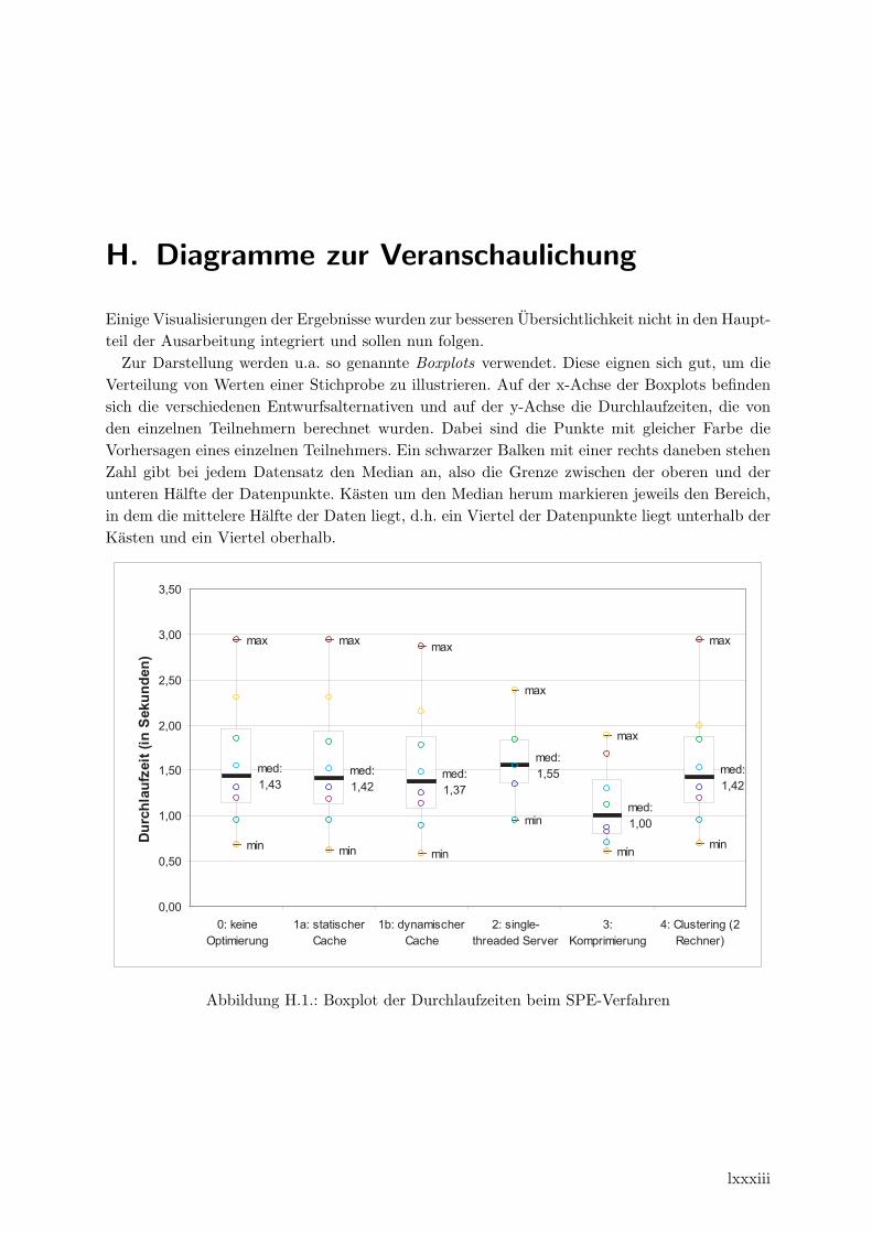
H. Diagramme zur Veranschaulichung
Einige Visualisierungen der Ergebnisse wurden zur besseren Ubersichtlichkeit nicht in den Haupt-teil der Ausarbeitung integriert und sollen nun folgen.
Zur Darstellung werden u.a. so genannte Boxplots verwendet. Diese eignen sich gut, um dieVerteilung von Werten einer Stichprobe zu illustrieren. Auf der x-Achse der Boxplots befindensich die verschiedenen Entwurfsalternativen und auf der y-Achse die Durchlaufzeiten, die vonden einzelnen Teilnehmern berechnet wurden. Dabei sind die Punkte mit gleicher Farbe dieVorhersagen eines einzelnen Teilnehmers. Ein schwarzer Balken mit einer rechts daneben stehenZahl gibt bei jedem Datensatz den Median an, also die Grenze zwischen der oberen und derunteren Halfte der Datenpunkte. Kasten um den Median herum markieren jeweils den Bereich,in dem die mittelere Halfte der Daten liegt, d.h. ein Viertel der Datenpunkte liegt unterhalb derKasten und ein Viertel oberhalb.
min min min
min
min min
med:1,43
med:1,42
med:1,37
med:1,55
med:1,00
med:1,42
max max max
max
max
max
0,00
0,50
1,00
1,50
2,00
2,50
3,00
3,50
0: keineOptimierung
1a: statischerCache
1b: dynamischerCache
2: single-threaded Server
3:Komprimierung
4: Clustering (2Rechner)
Durc
hlau
fzei
t (in
Sek
unde
n)
Abbildung H.1.: Boxplot der Durchlaufzeiten beim SPE-Verfahren
lxxxiii
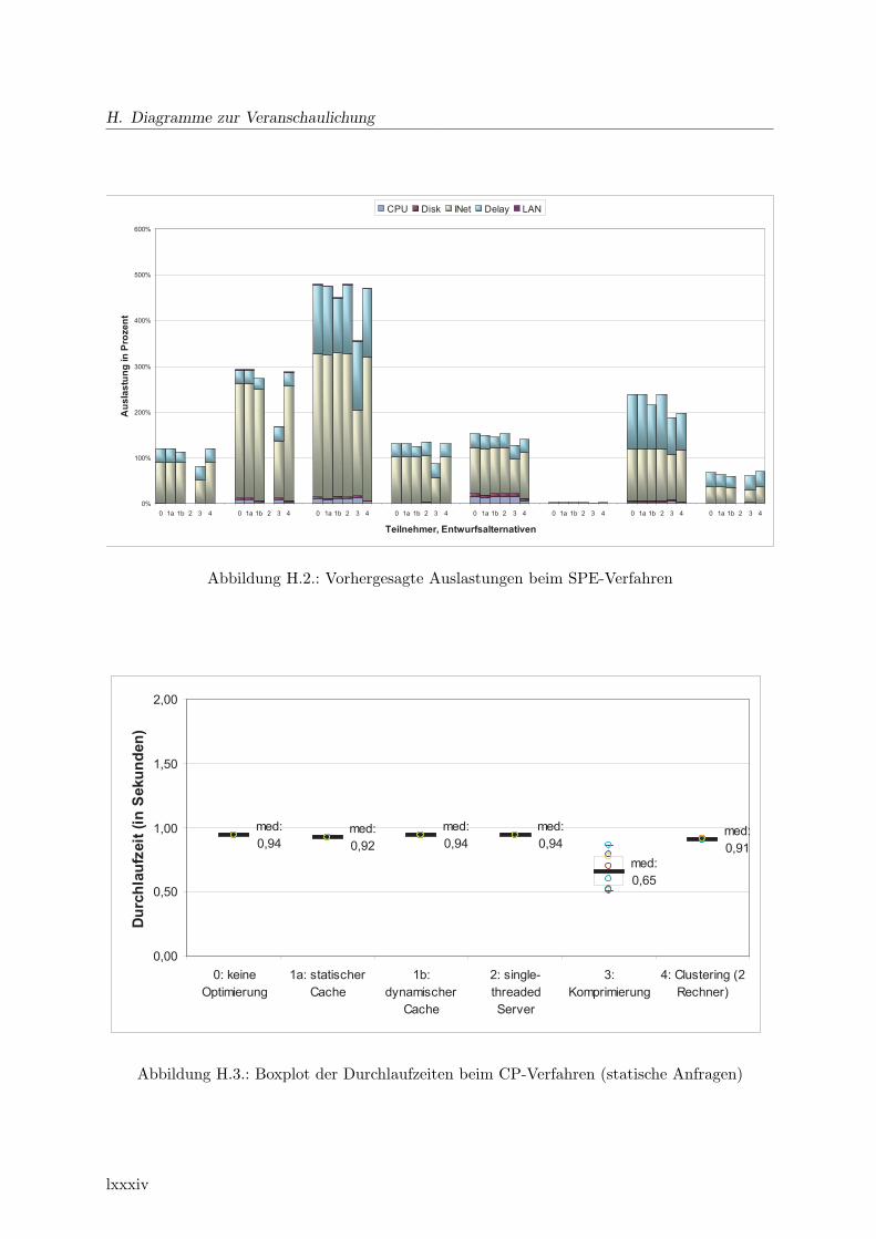
H. Diagramme zur Veranschaulichung
0%
100%
200%
300%
400%
500%
600%
0 1a 1b 2 3 4 0 1a 1b 2 3 4 0 1a 1b 2 3 4 0 1a 1b 2 3 4 0 1a 1b 2 3 4 0 1a 1b 2 3 4 0 1a 1b 2 3 4 0 1a 1b 2 3 4
Teilnehmer, Entwurfsalternativen
Aus
last
ung
in P
roze
nt
CPU Disk INet Delay LAN
Abbildung H.2.: Vorhergesagte Auslastungen beim SPE-Verfahren
med:0,94
med:0,92
med:0,94
med:0,94
med:0,65
med:0,91
0,00
0,50
1,00
1,50
2,00
0: keineOptimierung
1a: statischerCache
1b:dynamischer
Cache
2: single-threadedServer
3:Komprimierung
4: Clustering (2Rechner)
Durc
hlau
fzei
t (in
Sek
unde
n)
Abbildung H.3.: Boxplot der Durchlaufzeiten beim CP-Verfahren (statische Anfragen)
lxxxiv
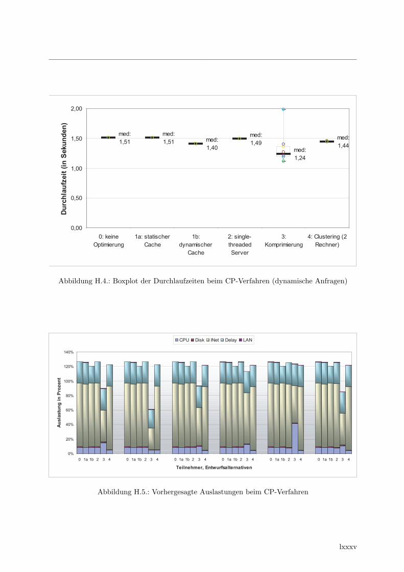
med:1,51
med:1,51 med:
1,40
med:1,49
med:1,24
med:1,44
0,00
0,50
1,00
1,50
2,00
0: keineOptimierung
1a: statischerCache
1b:dynamischer
Cache
2: single-threadedServer
3:Komprimierung
4: Clustering (2Rechner)
Durc
hlau
fzei
t (in
Sek
unde
n)
Abbildung H.4.: Boxplot der Durchlaufzeiten beim CP-Verfahren (dynamische Anfragen)
0%
20%
40%
60%
80%
100%
120%
140%
0 1a 1b 2 3 4 0 1a 1b 2 3 4 0 1a 1b 2 3 4 0 1a 1b 2 3 4 0 1a 1b 2 3 4 0 1a 1b 2 3 4
Teilnehmer, Entwurfsalternativen
Ausl
astu
ng in
Pro
zent
CPU Disk INet Delay LAN
Abbildung H.5.: Vorhergesagte Auslastungen beim CP-Verfahren
lxxxv
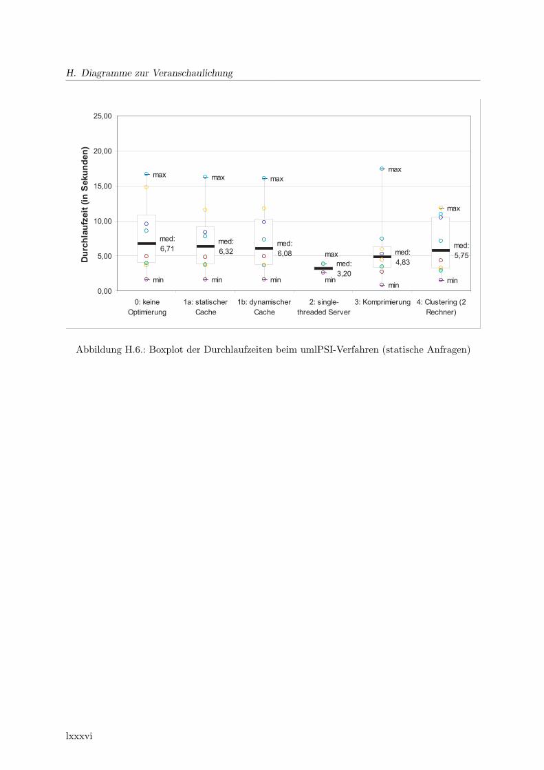
H. Diagramme zur Veranschaulichung
min min minmin min
med:6,71
med:6,32
med:6,08
med:3,20
med:4,83
med:5,75
max max maxmax
max
min
max
0,00
5,00
10,00
15,00
20,00
25,00
0: keineOptimierung
1a: statischerCache
1b: dynamischerCache
2: single-threaded Server
3: Komprimierung 4: Clustering (2Rechner)
Durc
hlau
fzei
t (in
Sek
unde
n)
Abbildung H.6.: Boxplot der Durchlaufzeiten beim umlPSI-Verfahren (statische Anfragen)
lxxxvi

min min minmin
minmin
med:9,67
med:9,60 med:
8,49
med:4,66
med:6,58
med:8,87
max max maxmax
max
max
0,00
5,00
10,00
15,00
20,00
25,00
0: keineOptimierung
1a: statischerCache
1b: dynamischerCache
2: single-threaded Server
3: Komprimierung 4: Clustering (2Rechner)
Durc
hlau
fzei
t (in
Sek
unde
n)
Abbildung H.7.: Boxplot der Durchlaufzeiten beim umlPSI-Verfahren (dynamische Anfragen)
0%
50%
100%
150%
200%
250%
0 1a 1b 2 3 4 0 1a 1b 2 3 4 0 1a 1b 2 3 4 0 1a 1b 2 3 4 0 1a 1b 2 3 4 0 1a 1b 2 3 4 0 1a 1b 2 3 4 0 1a 1b 2 3 4
Teilnehmer, Entwurfsalternativen
Aus
last
ung
in P
roze
nt
CPU Disk INet Delay LAN Threads
Abbildung H.8.: Vorhergesagte Auslastungen beim umlPSI-Verfahren
lxxxvii

lxxxviii
I. Messungen am Prototypen
Die Peformance-Messung des im Experiment untersuchten Webservers wird in Abschnitt 3.3naher erlautert. Es folgen die Rohdaten dieser Messungen. Die ausgewerteten Ergebnisse findensich in Abschnitt 4.1.4.
lxxxix
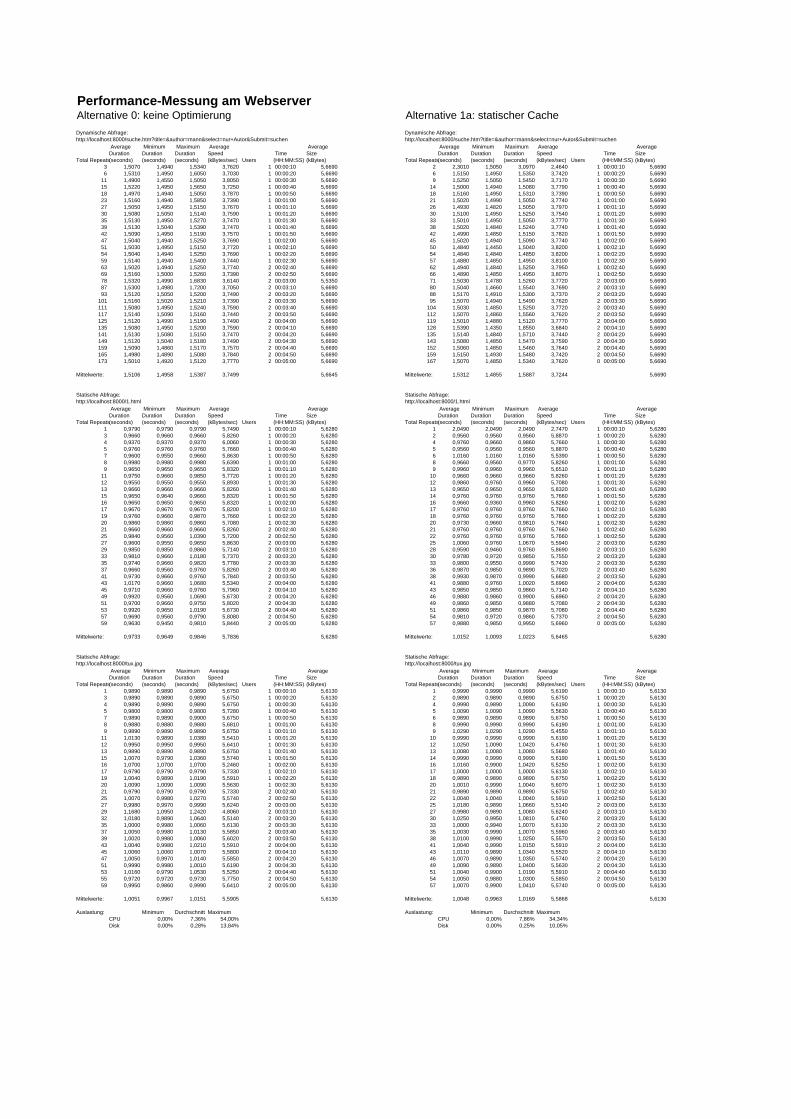
Performance-Messung am WebserverAlternative 0: keine Optimierung Alternative 1a: statischer CacheDynamische Abfrage: Dynamische Abfrage:http://localhost:8000/suche.htm?title=&author=mann&select=nur+Autor&Submit=suchen http://localhost:8000/suche.htm?title=&author=mann&select=nur+Autor&Submit=suchen
Total Repeats
Average Duration (seconds)
Minimum Duration (seconds)
Maximum Duration (seconds)
Average Speed (kBytes/sec) Users
Time (HH:MM:SS)
Average Size (kBytes) Total Repeats
Average Duration (seconds)
Minimum Duration (seconds)
Maximum Duration (seconds)
Average Speed (kBytes/sec) Users
Time (HH:MM:SS)
Average Size (kBytes)
3 1,5070 1,4940 1,5340 3,7620 1 00:00:10 5,6690 2 2,3010 1,5050 3,0970 2,4640 1 00:00:10 5,66906 1,5310 1,4950 1,6050 3,7030 1 00:00:20 5,6690 6 1,5150 1,4950 1,5350 3,7420 1 00:00:20 5,6690
11 1,4900 1,4550 1,5050 3,8050 1 00:00:30 5,6690 9 1,5250 1,5050 1,5450 3,7170 1 00:00:30 5,669015 1,5220 1,4950 1,5650 3,7250 1 00:00:40 5,6690 14 1,5000 1,4940 1,5080 3,7790 1 00:00:40 5,669018 1,4970 1,4940 1,5050 3,7870 1 00:00:50 5,6690 18 1,5160 1,4950 1,5310 3,7390 1 00:00:50 5,669023 1,5160 1,4940 1,5850 3,7390 1 00:01:00 5,6690 21 1,5020 1,4990 1,5050 3,7740 1 00:01:00 5,669027 1,5050 1,4950 1,5150 3,7670 1 00:01:10 5,6690 26 1,4930 1,4820 1,5050 3,7970 1 00:01:10 5,669030 1,5080 1,5050 1,5140 3,7590 1 00:01:20 5,6690 30 1,5100 1,4950 1,5250 3,7540 1 00:01:20 5,669035 1,5130 1,4950 1,5270 3,7470 1 00:01:30 5,6690 33 1,5010 1,4950 1,5050 3,7770 1 00:01:30 5,669039 1,5130 1,5040 1,5390 3,7470 1 00:01:40 5,6690 38 1,5020 1,4840 1,5240 3,7740 1 00:01:40 5,669042 1,5090 1,4950 1,5190 3,7570 1 00:01:50 5,6690 42 1,4990 1,4850 1,5150 3,7820 1 00:01:50 5,669047 1,5040 1,4940 1,5250 3,7690 1 00:02:00 5,6690 45 1,5020 1,4940 1,5090 3,7740 1 00:02:00 5,669051 1,5030 1,4950 1,5150 3,7720 1 00:02:10 5,6690 50 1,4840 1,4450 1,5040 3,8200 1 00:02:10 5,669054 1,5040 1,4940 1,5250 3,7690 1 00:02:20 5,6690 54 1,4840 1,4840 1,4850 3,8200 1 00:02:20 5,669059 1,5140 1,4940 1,5400 3,7440 1 00:02:30 5,6690 57 1,4880 1,4850 1,4950 3,8100 1 00:02:30 5,669063 1,5020 1,4940 1,5250 3,7740 2 00:02:40 5,6690 62 1,4940 1,4840 1,5250 3,7950 1 00:02:40 5,669069 1,5160 1,5000 1,5260 3,7390 2 00:02:50 5,6690 66 1,4890 1,4850 1,4950 3,8070 1 00:02:50 5,669078 1,5320 1,4990 1,6830 3,6140 2 00:03:00 5,5350 71 1,5030 1,4780 1,5260 3,7720 2 00:03:00 5,669087 1,5300 1,4980 1,7200 3,7050 2 00:03:10 5,6690 80 1,5040 1,4660 1,5540 3,7690 2 00:03:10 5,669093 1,5120 1,5050 1,5200 3,7490 2 00:03:20 5,6690 88 1,5170 1,4910 1,5300 3,7370 2 00:03:20 5,6690
101 1,5160 1,5020 1,5210 3,7390 2 00:03:30 5,6690 95 1,5070 1,4940 1,5490 3,7620 2 00:03:30 5,6690111 1,5080 1,4950 1,5240 3,7590 2 00:03:40 5,6690 104 1,5030 1,4850 1,5250 3,7720 2 00:03:40 5,6690117 1,5140 1,5090 1,5160 3,7440 2 00:03:50 5,6690 112 1,5070 1,4860 1,5560 3,7620 2 00:03:50 5,6690125 1,5120 1,4990 1,5190 3,7490 2 00:04:00 5,6690 119 1,5010 1,4880 1,5120 3,7770 2 00:04:00 5,6690135 1,5080 1,4950 1,5200 3,7590 2 00:04:10 5,6690 128 1,5390 1,4350 1,8550 3,6840 2 00:04:10 5,6690141 1,5130 1,5080 1,5150 3,7470 2 00:04:20 5,6690 135 1,5140 1,4840 1,5710 3,7440 2 00:04:20 5,6690149 1,5120 1,5040 1,5180 3,7490 2 00:04:30 5,6690 143 1,5080 1,4850 1,5470 3,7590 2 00:04:30 5,6690159 1,5090 1,4860 1,5170 3,7570 2 00:04:40 5,6690 152 1,5060 1,4850 1,5460 3,7640 2 00:04:40 5,6690165 1,4980 1,4890 1,5080 3,7840 2 00:04:50 5,6690 159 1,5150 1,4930 1,5480 3,7420 2 00:04:50 5,6690173 1,5010 1,4920 1,5120 3,7770 2 00:05:00 5,6690 167 1,5070 1,4850 1,5340 3,7620 0 00:05:00 5,6690
Mittelwerte: 1,5106 1,4958 1,5387 3,7499 5,6645 Mittelwerte: 1,5312 1,4855 1,5887 3,7244 5,6690
Statische Abfrage: Statische Abfrage:http://localhost:8000/1.html http://localhost:8000/1.html
Total Repeats
Average Duration (seconds)
Minimum Duration (seconds)
Maximum Duration (seconds)
Average Speed (kBytes/sec) Users
Time (HH:MM:SS)
Average Size (kBytes) Total Repeats
Average Duration (seconds)
Minimum Duration (seconds)
Maximum Duration (seconds)
Average Speed (kBytes/sec) Users
Time (HH:MM:SS)
Average Size (kBytes)
1 0,9790 0,9790 0,9790 5,7490 1 00:00:10 5,6280 1 2,0490 2,0490 2,0490 2,7470 1 00:00:10 5,62803 0,9660 0,9660 0,9660 5,8260 1 00:00:20 5,6280 2 0,9560 0,9560 0,9560 5,8870 1 00:00:20 5,62804 0,9370 0,9370 0,9370 6,0060 1 00:00:30 5,6280 4 0,9760 0,9660 0,9860 5,7660 1 00:00:30 5,62805 0,9760 0,9760 0,9760 5,7660 1 00:00:40 5,6280 5 0,9560 0,9560 0,9560 5,8870 1 00:00:40 5,62807 0,9600 0,9550 0,9660 5,8630 1 00:00:50 5,6280 6 1,0160 1,0160 1,0160 5,5390 1 00:00:50 5,62808 0,9980 0,9980 0,9980 5,6390 1 00:01:00 5,6280 8 0,9660 0,9560 0,9770 5,8260 1 00:01:00 5,62809 0,9650 0,9650 0,9650 5,8320 1 00:01:10 5,6280 9 0,9960 0,9960 0,9960 5,6510 1 00:01:10 5,6280
11 0,9750 0,9660 0,9850 5,7720 1 00:01:20 5,6280 10 0,9660 0,9660 0,9660 5,8260 1 00:01:20 5,628012 0,9550 0,9550 0,9550 5,8930 1 00:01:30 5,6280 12 0,9860 0,9760 0,9960 5,7080 1 00:01:30 5,628013 0,9660 0,9660 0,9660 5,8260 1 00:01:40 5,6280 13 0,9650 0,9650 0,9650 5,8320 1 00:01:40 5,628015 0,9650 0,9640 0,9660 5,8320 1 00:01:50 5,6280 14 0,9760 0,9760 0,9760 5,7660 1 00:01:50 5,628016 0,9650 0,9650 0,9650 5,8320 1 00:02:00 5,6280 16 0,9660 0,9360 0,9960 5,8260 1 00:02:00 5,628017 0,9670 0,9670 0,9670 5,8200 1 00:02:10 5,6280 17 0,9760 0,9760 0,9760 5,7660 1 00:02:10 5,628019 0,9760 0,9660 0,9870 5,7660 1 00:02:20 5,6280 18 0,9760 0,9760 0,9760 5,7660 1 00:02:20 5,628020 0,9860 0,9860 0,9860 5,7080 1 00:02:30 5,6280 20 0,9730 0,9660 0,9810 5,7840 1 00:02:30 5,628021 0,9660 0,9660 0,9660 5,8260 2 00:02:40 5,6280 21 0,9760 0,9760 0,9760 5,7660 1 00:02:40 5,628025 0,9840 0,9560 1,0390 5,7200 2 00:02:50 5,6280 22 0,9760 0,9760 0,9760 5,7660 1 00:02:50 5,628027 0,9600 0,9550 0,9650 5,8630 2 00:03:00 5,6280 25 1,0060 0,9760 1,0670 5,5940 2 00:03:00 5,628029 0,9850 0,9850 0,9860 5,7140 2 00:03:10 5,6280 28 0,9590 0,9460 0,9760 5,8690 2 00:03:10 5,628033 0,9810 0,9660 1,0180 5,7370 2 00:03:20 5,6280 30 0,9780 0,9720 0,9850 5,7550 2 00:03:20 5,628035 0,9740 0,9660 0,9820 5,7780 2 00:03:30 5,6280 33 0,9800 0,9550 0,9990 5,7430 2 00:03:30 5,628037 0,9660 0,9560 0,9760 5,8260 2 00:03:40 5,6280 36 0,9870 0,9850 0,9890 5,7020 2 00:03:40 5,628041 0,9730 0,9660 0,9760 5,7840 2 00:03:50 5,6280 38 0,9930 0,9870 0,9990 5,6680 2 00:03:50 5,628043 1,0170 0,9660 1,0680 5,5340 2 00:04:00 5,6280 41 0,9880 0,9760 1,0020 5,6960 2 00:04:00 5,628045 0,9710 0,9660 0,9760 5,7960 2 00:04:10 5,6280 43 0,9850 0,9850 0,9860 5,7140 2 00:04:10 5,628049 0,9920 0,9560 1,0690 5,6730 2 00:04:20 5,6280 46 0,9880 0,9860 0,9900 5,6960 2 00:04:20 5,628051 0,9700 0,9660 0,9750 5,8020 2 00:04:30 5,6280 49 0,9860 0,9850 0,9880 5,7080 2 00:04:30 5,628053 0,9920 0,9650 1,0190 5,6730 2 00:04:40 5,6280 51 0,9860 0,9850 0,9870 5,7080 2 00:04:40 5,628057 0,9690 0,9560 0,9790 5,8080 2 00:04:50 5,6280 54 0,9810 0,9720 0,9860 5,7370 2 00:04:50 5,628059 0,9630 0,9450 0,9810 5,8440 2 00:05:00 5,6280 57 0,9880 0,9850 0,9950 5,6960 0 00:05:00 5,6280
Mittelwerte: 0,9733 0,9649 0,9846 5,7836 5,6280 Mittelwerte: 1,0152 1,0093 1,0223 5,6465 5,6280
Statische Abfrage: Statische Abfrage:http://localhost:8000/tux.jpg http://localhost:8000/tux.jpg
Total Repeats
Average Duration (seconds)
Minimum Duration (seconds)
Maximum Duration (seconds)
Average Speed (kBytes/sec) Users
Time (HH:MM:SS)
Average Size (kBytes) Total Repeats
Average Duration (seconds)
Minimum Duration (seconds)
Maximum Duration (seconds)
Average Speed (kBytes/sec) Users
Time (HH:MM:SS)
Average Size (kBytes)
1 0,9890 0,9890 0,9890 5,6750 1 00:00:10 5,6130 1 0,9990 0,9990 0,9990 5,6190 1 00:00:10 5,61303 0,9890 0,9890 0,9890 5,6750 1 00:00:20 5,6130 2 0,9890 0,9890 0,9890 5,6750 1 00:00:20 5,61304 0,9890 0,9890 0,9890 5,6750 1 00:00:30 5,6130 4 0,9990 0,9890 1,0090 5,6190 1 00:00:30 5,61305 0,9800 0,9800 0,9800 5,7280 1 00:00:40 5,6130 5 1,0090 1,0090 1,0090 5,5630 1 00:00:40 5,61307 0,9890 0,9890 0,9900 5,6750 1 00:00:50 5,6130 6 0,9890 0,9890 0,9890 5,6750 1 00:00:50 5,61308 0,9880 0,9880 0,9880 5,6810 1 00:01:00 5,6130 8 0,9990 0,9990 0,9990 5,6190 1 00:01:00 5,61309 0,9890 0,9890 0,9890 5,6750 1 00:01:10 5,6130 9 1,0290 1,0290 1,0290 5,4550 1 00:01:10 5,6130
11 1,0130 0,9890 1,0380 5,5410 1 00:01:20 5,6130 10 0,9990 0,9990 0,9990 5,6190 1 00:01:20 5,613012 0,9950 0,9950 0,9950 5,6410 1 00:01:30 5,6130 12 1,0250 1,0090 1,0420 5,4760 1 00:01:30 5,613013 0,9890 0,9890 0,9890 5,6750 1 00:01:40 5,6130 13 1,0080 1,0080 1,0080 5,5680 1 00:01:40 5,613015 1,0070 0,9790 1,0360 5,5740 1 00:01:50 5,6130 14 0,9990 0,9990 0,9990 5,6190 1 00:01:50 5,613016 1,0700 1,0700 1,0700 5,2460 1 00:02:00 5,6130 16 1,0160 0,9900 1,0420 5,5250 1 00:02:00 5,613017 0,9790 0,9790 0,9790 5,7330 1 00:02:10 5,6130 17 1,0000 1,0000 1,0000 5,6130 1 00:02:10 5,613019 1,0040 0,9890 1,0190 5,5910 1 00:02:20 5,6130 18 0,9890 0,9890 0,9890 5,6750 1 00:02:20 5,613020 1,0090 1,0090 1,0090 5,5630 1 00:02:30 5,6130 20 1,0010 0,9990 1,0040 5,6070 1 00:02:30 5,613021 0,9790 0,9790 0,9790 5,7330 2 00:02:40 5,6130 21 0,9890 0,9890 0,9890 5,6750 1 00:02:40 5,613025 1,0070 0,9980 1,0270 5,5740 2 00:02:50 5,6130 22 1,0040 1,0040 1,0040 5,5910 1 00:02:50 5,613027 0,9980 0,9970 0,9990 5,6240 2 00:03:00 5,6130 25 1,0180 0,9890 1,0660 5,5140 2 00:03:00 5,613029 1,1680 1,0950 1,2420 4,8060 2 00:03:10 5,6130 27 0,9980 0,9890 1,0080 5,6240 2 00:03:10 5,613032 1,0180 0,9890 1,0640 5,5140 2 00:03:20 5,6130 30 1,0250 0,9950 1,0810 5,4760 2 00:03:20 5,613035 1,0000 0,9980 1,0060 5,6130 2 00:03:30 5,6130 33 1,0000 0,9940 1,0070 5,6130 2 00:03:30 5,613037 1,0050 0,9980 1,0130 5,5850 2 00:03:40 5,6130 35 1,0030 0,9990 1,0070 5,5960 2 00:03:40 5,613039 1,0020 0,9980 1,0060 5,6020 2 00:03:50 5,6130 38 1,0100 0,9990 1,0250 5,5570 2 00:03:50 5,613043 1,0040 0,9980 1,0210 5,5910 2 00:04:00 5,6130 41 1,0040 0,9990 1,0150 5,5910 2 00:04:00 5,613045 1,0060 1,0060 1,0070 5,5800 2 00:04:10 5,6130 43 1,0110 0,9890 1,0340 5,5520 2 00:04:10 5,613047 1,0050 0,9970 1,0140 5,5850 2 00:04:20 5,6130 46 1,0070 0,9890 1,0350 5,5740 2 00:04:20 5,613051 0,9990 0,9980 1,0010 5,6190 2 00:04:30 5,6130 49 1,0090 0,9890 1,0400 5,5630 2 00:04:30 5,613053 1,0160 0,9790 1,0530 5,5250 2 00:04:40 5,6130 51 1,0040 0,9900 1,0190 5,5910 2 00:04:40 5,613055 0,9720 0,9720 0,9730 5,7750 2 00:04:50 5,6130 54 1,0050 0,9880 1,0300 5,5850 2 00:04:50 5,613059 0,9950 0,9860 0,9990 5,6410 2 00:05:00 5,6130 57 1,0070 0,9900 1,0410 5,5740 0 00:05:00 5,6130
Mittelwerte: 1,0051 0,9967 1,0151 5,5905 5,6130 Mittelwerte: 1,0048 0,9963 1,0169 5,5868 5,6130
Auslastung: Minimum Durchschnitt Maximum Auslastung: Minimum Durchschnitt MaximumCPU 0,00% 7,36% 54,00% CPU 0,00% 7,86% 34,34%Disk 0,00% 0,28% 13,84% Disk 0,00% 0,25% 10,05%
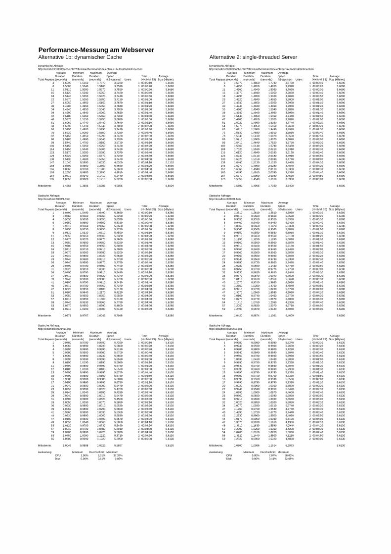
Performance-Messung am WebserverAlternative 1b: dynamischer Cache Alternative 2: single-threaded ServerDynamische Abfrage: Dynamische Abfrage:http://localhost:8000/suche.htm?title=&author=mann&select=nur+Autor&Submit=suchen http://localhost:8000/suche.htm?title=&author=mann&select=nur+Autor&Submit=suchen
Total Repeats
Average Duration (seconds)
Minimum Duration (seconds)
Maximum Duration (seconds)
Average Speed (kBytes/sec) Users
Time (HH:MM:SS)
Average Size (kBytes) Total Repeats
Average Duration (seconds)
Minimum Duration (seconds)
Maximum Duration (seconds)
Average Speed (kBytes/sec) Users
Time (HH:MM:SS)
Average Size (kBytes)
3 1,6090 1,5150 1,7970 3,5230 1 00:00:10 5,6690 3 1,5870 1,4850 1,7740 3,5720 1 00:00:10 5,66906 1,5080 1,5040 1,5180 3,7590 1 00:00:20 5,6690 6 1,4950 1,4950 1,4950 3,7920 1 00:00:20 5,6690
11 1,5110 1,5050 1,5270 3,7520 1 00:00:30 5,6690 11 1,4960 1,4940 1,5050 3,7890 1 00:00:30 5,669015 1,5120 1,5040 1,5250 3,7490 1 00:00:40 5,6690 15 1,4970 1,4940 1,5050 3,7870 1 00:00:40 5,669018 1,5140 1,5050 1,5320 3,7440 1 00:00:50 5,6690 18 1,4990 1,4950 1,5100 3,7820 1 00:00:50 5,669022 1,5270 1,5050 1,5850 3,7130 1 00:01:00 5,6690 23 1,4920 1,4840 1,4950 3,8000 1 00:01:00 5,669027 1,5050 1,4950 1,5150 3,7670 1 00:01:10 5,6690 27 1,4940 1,4850 1,5050 3,7950 1 00:01:10 5,669030 1,4980 1,4950 1,5050 3,7840 1 00:01:20 5,6690 30 1,4940 1,4940 1,4950 3,7950 1 00:01:20 5,669034 1,4940 1,4850 1,5040 3,7950 1 00:01:30 5,6690 35 1,4960 1,4940 1,5040 3,7890 1 00:01:30 5,669039 1,4990 1,4940 1,5060 3,7820 1 00:01:40 5,6690 39 1,4940 1,4940 1,4950 3,7950 1 00:01:40 5,669042 1,5180 1,5050 1,5460 3,7350 1 00:01:50 5,6690 42 1,5140 1,4950 1,5450 3,7440 1 00:01:50 5,669046 1,5370 1,5150 1,5750 3,6880 1 00:02:00 5,6690 47 1,4960 1,4950 1,5050 3,7890 1 00:02:00 5,669051 1,5060 1,4740 1,5440 3,7640 2 00:02:10 5,6690 51 1,5020 1,4950 1,5150 3,7740 1 00:02:10 5,669058 1,5290 1,5110 1,5640 3,7080 2 00:02:20 5,6690 54 1,5070 1,4950 1,5150 3,7620 2 00:02:20 5,669066 1,5150 1,4800 1,5790 3,7420 2 00:02:30 5,6690 63 1,6210 1,5680 1,9490 3,4970 2 00:02:30 5,669075 1,5220 1,5050 1,5550 3,7250 2 00:02:40 5,6690 72 1,5830 1,4880 1,6910 3,5810 2 00:02:40 5,669082 1,5150 1,4950 1,5290 3,7420 2 00:02:50 5,6690 78 1,5940 1,5410 1,6070 3,5560 2 00:02:50 5,669090 1,5180 1,4990 1,5540 3,7350 2 00:03:00 5,6690 86 1,5710 1,5000 1,6070 3,6090 2 00:03:00 5,669099 1,5440 1,4700 1,8180 3,6720 2 00:03:10 5,6690 95 1,5410 1,4640 1,7520 3,6790 2 00:03:10 5,6690
106 1,5150 1,5050 1,5250 3,7420 2 00:03:20 5,6690 102 1,5560 1,5140 1,5790 3,6430 2 00:03:20 5,6690114 1,5150 1,5040 1,5300 3,7420 2 00:03:30 5,6690 108 1,7020 1,5530 2,0210 3,3310 2 00:03:30 5,6690123 1,5170 1,5050 1,5390 3,7370 2 00:03:40 5,6690 116 1,6120 1,4840 2,0190 3,5170 2 00:03:40 5,6690129 1,5220 1,5050 1,5570 3,7250 2 00:03:50 5,6690 123 1,6240 1,5110 2,0180 3,4910 2 00:03:50 5,6690138 1,5130 1,4580 1,5950 3,7470 2 00:04:00 5,6690 130 1,6320 1,5150 2,0590 3,4740 2 00:04:00 5,6690147 1,1040 0,5890 1,6030 4,6300 2 00:04:10 5,1110 138 1,6440 1,5130 2,1150 3,4480 2 00:04:10 5,6690158 1,0390 0,9660 1,2660 5,4560 2 00:04:20 5,6690 145 1,6270 1,4950 2,0280 3,4840 2 00:04:20 5,6690166 1,0560 0,9700 1,1200 5,3680 2 00:04:30 5,6690 152 1,6060 1,4940 2,0110 3,5300 2 00:04:30 5,6690176 1,2650 0,9800 2,3790 4,4810 2 00:04:40 5,6690 160 1,6490 1,4910 2,0390 3,4380 2 00:04:40 5,6690184 1,0810 0,9940 1,1410 5,2440 2 00:04:50 5,6690 167 1,6370 1,5050 2,0980 3,4630 2 00:04:50 5,6690195 1,0650 0,9820 1,1210 5,3230 0 00:05:00 5,6690 173 1,5350 1,4540 1,6150 3,6930 2 00:05:00 5,6690
Mittelwerte: 1,4358 1,3806 1,5385 4,0025 5,6504 Mittelwerte: 1,5599 1,4995 1,7190 3,6400 5,6690
Statische Abfrage: Statische Abfrage:http://localhost:8000/1.html http://localhost:8000/1.html
Total Repeats
Average Duration (seconds)
Minimum Duration (seconds)
Maximum Duration (seconds)
Average Speed (kBytes/sec) Users
Time (HH:MM:SS)
Average Size (kBytes) Total Repeats
Average Duration (seconds)
Minimum Duration (seconds)
Maximum Duration (seconds)
Average Speed (kBytes/sec) Users
Time (HH:MM:SS)
Average Size (kBytes)
1 1,0490 1,0490 1,0490 5,3650 1 00:00:10 5,6280 1 1,2810 1,2810 1,2810 4,3930 1 00:00:10 5,62803 0,9660 0,9560 0,9760 5,8260 1 00:00:20 5,6280 3 0,9610 0,9560 0,9660 5,8560 1 00:00:20 5,62804 0,9650 0,9650 0,9650 5,8320 1 00:00:30 5,6280 4 0,9550 0,9550 0,9550 5,8930 1 00:00:30 5,62805 0,9650 0,9650 0,9650 5,8320 1 00:00:40 5,6280 5 0,9460 0,9460 0,9460 5,9490 1 00:00:40 5,62807 0,9610 0,9560 0,9660 5,8560 1 00:00:50 5,6280 7 1,0560 0,9660 1,1470 5,3300 1 00:00:50 5,62808 0,9750 0,9750 0,9750 5,7720 1 00:01:00 5,6280 8 0,9560 0,9560 0,9560 5,8870 1 00:01:00 5,62809 1,0310 1,0310 1,0310 5,4590 1 00:01:10 5,6280 9 0,9550 0,9550 0,9550 5,8930 1 00:01:10 5,6280
11 0,9650 0,9650 0,9660 5,8320 1 00:01:20 5,6280 11 0,9510 0,9460 0,9560 5,9180 1 00:01:20 5,628012 0,9770 0,9770 0,9770 5,7600 1 00:01:30 5,6280 12 1,1250 1,1250 1,1250 5,0030 1 00:01:30 5,628013 0,9650 0,9650 0,9650 5,8320 1 00:01:40 5,6280 13 0,9560 0,9560 0,9560 5,8870 1 00:01:40 5,628015 0,9700 0,9550 0,9850 5,8020 1 00:01:50 5,6280 15 0,9510 0,9460 0,9560 5,9180 1 00:01:50 5,628016 0,9710 0,9710 0,9710 5,7960 1 00:02:00 5,6280 16 0,9460 0,9460 0,9460 5,9490 1 00:02:00 5,628018 0,9670 0,9560 0,9780 5,8200 2 00:02:10 5,6280 17 0,9560 0,9560 0,9560 5,8870 1 00:02:10 5,628021 0,9940 0,9800 1,0020 5,6620 2 00:02:20 5,6280 20 0,9760 0,9560 0,9960 5,7660 2 00:02:20 5,628023 0,9740 0,9680 0,9810 5,7780 2 00:02:30 5,6280 22 0,9640 0,9560 0,9730 5,8380 2 00:02:30 5,628026 0,9740 0,9690 0,9770 5,7780 2 00:02:40 5,6280 24 0,9790 0,9730 0,9860 5,7490 2 00:02:40 5,628029 0,9790 0,9780 0,9800 5,7490 2 00:02:50 5,6280 28 1,0280 0,9560 1,1420 5,4750 2 00:02:50 5,628031 0,9920 0,9810 1,0030 5,6730 2 00:03:00 5,6280 30 0,9750 0,9730 0,9770 5,7720 2 00:03:00 5,628034 0,9790 0,9790 0,9810 5,7490 2 00:03:10 5,6280 32 0,9630 0,9620 0,9650 5,8440 2 00:03:10 5,628037 0,9810 0,9800 0,9820 5,7370 2 00:03:20 5,6280 35 0,9770 0,9540 1,0040 5,7600 2 00:03:20 5,628039 0,9740 0,9690 0,9800 5,7780 2 00:03:30 5,6280 37 1,0110 0,9670 1,0550 5,5670 2 00:03:30 5,628041 0,9800 0,9790 0,9810 5,7430 2 00:03:40 5,6280 40 1,2070 0,9740 1,5860 4,6630 2 00:03:40 5,628045 0,9810 0,9780 0,9860 5,7370 2 00:03:50 5,6280 42 1,2550 1,0360 1,4750 4,4840 2 00:03:50 5,628047 1,0020 0,9950 1,0100 5,6170 2 00:04:00 5,6280 45 0,9910 0,9730 1,0260 5,6790 2 00:04:00 5,628051 1,0380 0,9640 1,2170 5,4220 2 00:04:10 5,6280 47 1,3070 1,0560 1,5580 4,3060 2 00:04:10 5,628053 0,9950 0,9650 1,0250 5,6560 2 00:04:20 5,6280 49 1,0100 0,9740 1,0460 5,5720 2 00:04:20 5,628057 1,0210 0,9650 1,1360 5,5120 2 00:04:30 5,6280 52 1,0270 0,9770 1,0670 5,4800 2 00:04:30 5,628059 0,9740 0,9530 0,9960 5,7780 2 00:04:40 5,6280 54 1,1410 1,0760 1,2060 4,9330 2 00:04:40 5,628063 1,0270 0,9950 1,0990 5,4800 2 00:04:50 5,6280 57 1,2050 0,9830 1,5070 4,6710 2 00:04:50 5,628066 1,0210 1,0160 1,0300 5,5120 0 00:05:00 5,6280 59 1,2490 0,9870 1,5120 4,5060 2 00:05:00 5,6280
Mittelwerte: 0,9871 0,9767 1,0045 5,7048 5,6280 Mittelwerte: 1,0420 0,9874 1,1061 5,4609 5,6280
Statische Abfrage: Statische Abfrage:http://localhost:8000/tux.jpg http://localhost:8000/tux.jpg
Total Repeats
Average Duration (seconds)
Minimum Duration (seconds)
Maximum Duration (seconds)
Average Speed (kBytes/sec) Users
Time (HH:MM:SS)
Average Size (kBytes) Total Repeats
Average Duration (seconds)
Minimum Duration (seconds)
Maximum Duration (seconds)
Average Speed (kBytes/sec) Users
Time (HH:MM:SS)
Average Size (kBytes)
1 0,9780 0,9780 0,9780 5,7390 1 00:00:10 5,6130 1 0,9980 0,9980 0,9980 5,6240 1 00:00:10 5,61303 1,0060 0,9890 1,0230 5,5800 1 00:00:20 5,6130 3 0,9740 0,9590 0,9900 5,7630 1 00:00:20 5,61304 0,9990 0,9990 0,9990 5,6190 1 00:00:30 5,6130 4 0,9800 0,9800 0,9800 5,7280 1 00:00:30 5,61305 0,9900 0,9900 0,9900 5,6700 1 00:00:40 5,6130 5 0,9840 0,9840 0,9840 5,7040 1 00:00:40 5,61307 1,0060 0,9890 1,0240 5,5800 1 00:00:50 5,6130 7 0,9860 0,9780 0,9950 5,6930 1 00:00:50 5,61308 0,9590 0,9590 0,9590 5,8530 1 00:01:00 5,6130 8 1,0430 1,0430 1,0430 5,3820 1 00:01:00 5,61309 1,0190 1,0190 1,0190 5,5080 1 00:01:10 5,6130 9 0,9790 0,9790 0,9790 5,7330 1 00:01:10 5,6130
11 0,9890 0,9890 0,9890 5,6750 1 00:01:20 5,6130 11 0,9840 0,9790 0,9890 5,7040 1 00:01:20 5,613012 1,0100 1,0100 1,0100 5,5570 1 00:01:30 5,6130 12 0,9690 0,9690 0,9690 5,7930 1 00:01:30 5,613013 0,9890 0,9890 0,9890 5,6750 1 00:01:40 5,6130 13 0,9790 0,9790 0,9790 5,7330 1 00:01:40 5,613015 0,9890 0,9680 1,0100 5,6750 1 00:01:50 5,6130 15 0,9790 0,9790 0,9790 5,7330 1 00:01:50 5,613016 0,9880 0,9880 0,9880 5,6810 1 00:02:00 5,6130 16 0,9590 0,9590 0,9590 5,8530 1 00:02:00 5,613017 0,9890 0,9890 0,9890 5,6750 2 00:02:10 5,6130 17 0,9790 0,9790 0,9790 5,7330 1 00:02:10 5,613021 0,9940 0,9890 1,0000 5,6470 2 00:02:20 5,6130 20 1,0020 0,9960 1,0100 5,6020 2 00:02:20 5,613023 1,0250 0,9890 1,0620 5,4760 2 00:02:30 5,6130 22 0,9940 0,9940 0,9950 5,6470 2 00:02:30 5,613025 1,0340 1,0040 1,0650 5,4280 2 00:02:40 5,6130 24 1,0280 1,0000 1,0570 5,4600 2 00:02:40 5,613029 0,9940 0,9890 1,0010 5,6470 2 00:02:50 5,6130 26 0,9860 0,9690 1,0040 5,6930 2 00:02:50 5,613031 1,0300 0,9980 1,0620 5,4500 2 00:03:00 5,6130 30 0,9910 0,9690 1,0060 5,6640 2 00:03:00 5,613033 1,0050 1,0030 1,0070 5,5850 2 00:03:10 5,6130 32 1,0020 0,9850 1,0200 5,6020 2 00:03:10 5,613036 0,9930 0,9890 1,0010 5,6530 2 00:03:20 5,6130 34 1,0070 1,0030 1,0110 5,5740 2 00:03:20 5,613039 1,0060 0,9890 1,0290 5,5800 2 00:03:30 5,6130 37 1,1760 0,9790 1,5540 4,7730 2 00:03:30 5,613041 0,9960 0,9890 1,0030 5,6360 2 00:03:40 5,6130 40 1,4990 1,2730 1,6770 3,7440 2 00:03:40 5,613044 0,9930 0,9890 1,0000 5,6530 2 00:03:50 5,6130 42 1,2730 0,9960 1,5500 4,4090 2 00:03:50 5,613047 1,0100 0,9590 1,0590 5,5570 2 00:04:00 5,6130 44 1,0170 0,9950 1,0390 5,5190 2 00:04:00 5,613049 1,0050 1,0040 1,0060 5,5850 2 00:04:10 5,6130 47 1,3570 0,9970 1,5650 4,1360 2 00:04:10 5,613053 1,0120 0,9700 1,0730 5,5460 2 00:04:20 5,6130 49 1,3710 1,1830 1,5590 4,0940 2 00:04:20 5,613057 1,0040 0,9700 1,0480 5,5910 2 00:04:30 5,6130 52 1,2700 1,0250 1,5350 4,4200 2 00:04:30 5,613059 1,0200 0,9990 1,0420 5,5030 2 00:04:40 5,6130 54 1,0200 1,0160 1,0250 5,5030 2 00:04:40 5,613063 1,0450 1,0090 1,1220 5,3710 2 00:04:50 5,6130 56 1,3620 1,1440 1,5800 4,1210 2 00:04:50 5,613065 1,0600 0,9990 1,1220 5,2950 0 00:05:00 5,6130 59 1,2520 0,9980 1,5320 4,4830 2 00:05:00 5,6130
Mittelwerte: 1,0046 0,9898 1,0223 5,5897 5,6130 Mittelwerte: 1,0800 1,0096 1,1514 5,2873 5,6130
Auslastung: Minimum Durchschnitt Maximum Auslastung: Minimum Durchschnitt MaximumCPU 1,00% 8,01% 37,37% CPU 0,00% 7,07% 58,00%Disk 0,00% 0,11% 0,85% Disk 0,00% 0,41% 22,68%
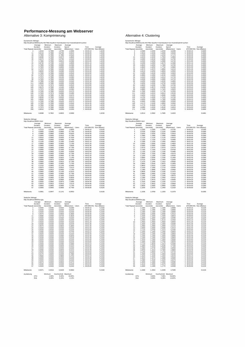
Performance-Messung am WebserverAlternative 3: Komprimierung Alternative 4: ClusteringDynamische Abfrage: Dynamische Abfrage:http://localhost:8000/suche.htm?title=&author=mann&select=nur+Autor&Submit=suchen http://localhost:8000/suche.htm?title=&author=mann&select=nur+Autor&Submit=suchen
Total Repeats
Average Duration (seconds)
Minimum Duration (seconds)
Maximum Duration (seconds)
Average Speed (kBytes/sec) Users
Time (HH:MM:SS)
Average Size (kBytes) Total Repeats
Average Duration (seconds)
Minimum Duration (seconds)
Maximum Duration (seconds)
Average Speed (kBytes/sec) Users
Time (HH:MM:SS)
Average Size (kBytes)
4 1,0210 0,7890 1,6790 1,5900 1 00:00:10 1,6230 3 1,5580 1,5250 1,6250 3,6390 1 00:00:10 5,669011 0,8110 0,7880 0,8790 2,0010 1 00:00:20 1,6230 6 1,5910 1,5240 1,6260 3,5630 1 00:00:20 5,669018 0,7900 0,7890 0,7990 2,0540 1 00:00:30 1,6230 9 1,5250 1,5250 1,5250 3,7170 1 00:00:30 5,669024 0,8280 0,7900 0,9370 1,9600 1 00:00:40 1,6230 14 1,6220 1,5240 1,7050 3,4950 1 00:00:40 5,669030 0,8470 0,7890 0,9780 1,9160 1 00:00:50 1,6230 18 1,6300 1,6240 1,6380 3,4780 1 00:00:50 5,669037 0,7960 0,7890 0,8010 2,0390 1 00:01:00 1,6230 21 1,6320 1,6250 1,6380 3,4740 1 00:01:00 5,669044 0,8730 0,7390 1,4220 1,8590 1 00:01:10 1,6230 24 1,6490 1,6350 1,6570 3,4380 1 00:01:10 5,669051 0,7960 0,7880 0,8090 2,0390 1 00:01:20 1,6230 28 1,6820 1,6250 1,7460 3,3700 1 00:01:20 5,669057 0,7920 0,7880 0,8000 2,0490 1 00:01:30 1,6230 32 1,6840 1,6250 1,7750 3,3660 1 00:01:30 5,669064 0,7970 0,7880 0,8180 2,0360 1 00:01:40 1,6230 36 1,6570 1,6370 1,6850 3,4210 1 00:01:40 5,669072 0,8020 0,7890 0,8390 2,0240 1 00:01:50 1,6230 39 1,6410 1,6250 1,6650 3,4550 1 00:01:50 5,669078 0,7900 0,7880 0,8000 2,0540 1 00:02:00 1,6230 42 1,6280 1,6240 1,6350 3,4820 1 00:02:00 5,669084 0,7870 0,7590 0,8080 2,0620 1 00:02:10 1,6230 48 1,6660 1,5260 1,9150 3,4030 2 00:02:10 5,669091 0,7970 0,7880 0,8190 2,0360 1 00:02:20 1,6230 56 1,6320 1,6290 1,6410 3,4740 2 00:02:20 5,669099 0,7920 0,7890 0,8100 2,0490 1 00:02:30 1,6230 63 1,6330 1,6280 1,6400 3,4720 2 00:02:30 5,6690
105 0,7980 0,7880 0,8200 2,0340 1 00:02:40 1,6230 69 1,6290 1,6280 1,6330 3,4800 2 00:02:40 5,6690111 0,8000 0,7880 0,8400 2,0290 1 00:02:50 1,6230 76 1,6450 1,6330 1,6750 3,4460 2 00:02:50 5,6690119 0,7910 0,7870 0,8000 2,0520 1 00:03:00 1,6230 84 1,6820 1,6330 1,7600 3,3700 2 00:03:00 5,6690126 0,8270 0,7890 1,0190 1,9630 1 00:03:10 1,6230 92 1,8160 1,6670 2,1030 3,1220 2 00:03:10 5,6690132 0,7970 0,7890 0,8190 2,0360 1 00:03:20 1,6230 99 1,6860 1,6290 1,7420 3,3620 2 00:03:20 5,6690138 0,7930 0,7880 0,8200 2,0470 1 00:03:30 1,6230 105 1,7000 1,6020 1,7740 3,3350 2 00:03:30 5,6690146 0,7920 0,7870 0,8080 2,0490 1 00:03:40 1,6230 111 1,9450 1,6310 3,4610 2,9150 2 00:03:40 5,6690153 0,7930 0,7890 0,7990 2,0470 1 00:03:50 1,6230 118 1,6450 1,6310 1,6580 3,4460 2 00:03:50 5,6690159 0,8030 0,7900 0,8200 2,0210 1 00:04:00 1,6230 126 1,6790 1,6330 1,7520 3,3760 2 00:04:00 5,6690165 0,8040 0,7700 0,8480 2,0190 1 00:04:10 1,6230 134 1,6490 1,5380 1,7380 3,4380 2 00:04:10 5,6690172 0,7930 0,7880 0,8100 2,0470 1 00:04:20 1,6230 141 1,5940 1,5360 1,6380 3,5560 2 00:04:20 5,6690180 0,7900 0,7890 0,8000 2,0540 1 00:04:30 1,6230 148 1,6170 1,5430 1,6800 3,5060 2 00:04:30 5,6690186 0,7950 0,7890 0,8090 2,0420 1 00:04:40 1,6230 156 1,4770 0,2640 1,7440 3,4130 2 00:04:40 5,0410192 0,7970 0,7880 0,8290 2,0360 1 00:04:50 1,6230 164 1,6380 1,6330 1,6530 3,4610 2 00:04:50 5,6690200 0,8010 0,7880 0,8360 2,0260 1 00:05:00 1,6230 171 1,7100 1,6450 1,9290 3,3150 0 00:05:00 5,6690
Mittelwerte: 0,8098 0,7852 0,8825 2,0090 1,6230 Mittelwerte: 1,6514 1,5582 1,7685 3,4263 5,6481
Statische Abfrage: Statische Abfrage:http://localhost:8000/1.html http://localhost:8000/1.html
Total Repeats
Average Duration (seconds)
Minimum Duration (seconds)
Maximum Duration (seconds)
Average Speed (kBytes/sec) Users
Time (HH:MM:SS)
Average Size (kBytes) Total Repeats
Average Duration (seconds)
Minimum Duration (seconds)
Maximum Duration (seconds)
Average Speed (kBytes/sec) Users
Time (HH:MM:SS)
Average Size (kBytes)
2 0,3210 0,0790 0,5640 1,9000 1 00:00:10 0,6100 1 1,2300 1,2300 1,2300 4,5760 1 00:00:10 5,62804 0,0900 0,0900 0,0900 6,7780 1 00:00:20 0,6100 3 1,0700 1,0250 1,1150 5,2600 1 00:00:20 5,62806 0,0880 0,0860 0,0900 6,9320 1 00:00:30 0,6100 4 1,0250 1,0250 1,0250 5,4910 1 00:00:30 5,62809 0,0900 0,0900 0,0910 6,7780 1 00:00:40 0,6100 5 1,1580 1,1580 1,1580 4,8600 1 00:00:40 5,6280
11 0,0910 0,0900 0,0930 6,7030 1 00:00:50 0,6100 6 1,1120 1,1120 1,1120 5,0610 1 00:00:50 5,628013 0,0900 0,0900 0,0900 6,7780 1 00:01:00 0,6100 7 1,1150 1,1150 1,1150 5,0480 1 00:01:00 5,628015 0,1100 0,0900 0,1300 5,5450 1 00:01:10 0,6100 9 1,1300 1,1150 1,1450 4,9810 1 00:01:10 5,628017 0,0850 0,0800 0,0900 7,1760 1 00:01:20 0,6100 10 1,0260 1,0260 1,0260 5,4850 1 00:01:20 5,628020 0,0860 0,0800 0,0900 7,0930 1 00:01:30 0,6100 11 1,0260 1,0260 1,0260 5,4850 1 00:01:30 5,628022 0,0900 0,0900 0,0900 6,7780 1 00:01:40 0,6100 12 1,0370 1,0370 1,0370 5,4270 1 00:01:40 5,628024 0,0950 0,0900 0,1000 6,4210 1 00:01:50 0,6100 13 1,1160 1,1160 1,1160 5,0430 1 00:01:50 5,628027 0,0930 0,0900 0,1000 6,5590 1 00:02:00 0,6100 15 1,1150 1,1150 1,1160 5,0480 1 00:02:00 5,628029 0,0900 0,0900 0,0900 6,7780 1 00:02:10 0,6100 17 1,1400 1,1320 1,1480 4,9370 2 00:02:10 5,628031 0,0900 0,0900 0,0900 6,7780 1 00:02:20 0,6100 19 1,1250 1,1180 1,1330 5,0030 2 00:02:20 5,628033 0,0850 0,0800 0,0910 7,1760 1 00:02:30 0,6100 22 1,0950 1,0330 1,1330 5,1400 2 00:02:30 5,628036 0,0890 0,0870 0,0900 6,8540 1 00:02:40 0,6100 25 1,0720 1,0340 1,1400 5,2500 2 00:02:40 5,628038 0,0900 0,0900 0,0910 6,7780 1 00:02:50 0,6100 27 1,1370 1,1340 1,1410 4,9500 2 00:02:50 5,628040 0,0850 0,0800 0,0900 7,1760 1 00:03:00 0,6100 29 1,0650 1,0340 1,0970 5,2850 2 00:03:00 5,628042 0,1010 0,0800 0,1230 6,0400 1 00:03:10 0,6100 31 1,0820 1,0310 1,1330 5,2010 2 00:03:10 5,628045 0,0870 0,0810 0,0910 7,0110 1 00:03:20 0,6100 34 1,1440 1,1260 1,1710 4,9200 2 00:03:20 5,628047 0,0850 0,0810 0,0900 7,1760 1 00:03:30 0,6100 37 1,1380 1,0680 1,2000 4,9460 2 00:03:30 5,628049 0,0950 0,0800 0,1100 6,4210 1 00:03:40 0,6100 39 1,0830 1,0340 1,1330 5,1970 2 00:03:40 5,628051 0,0900 0,0900 0,0900 6,7780 1 00:03:50 0,6100 41 1,0860 1,0400 1,1330 5,1820 2 00:03:50 5,628054 0,1030 0,0600 0,1600 5,9220 1 00:04:00 0,6100 43 1,1330 1,1330 1,1340 4,9670 2 00:04:00 5,628056 0,1200 0,0900 0,1500 5,0830 1 00:04:10 0,6100 45 1,1390 1,0340 1,2450 4,9410 2 00:04:10 5,628058 0,0880 0,0870 0,0900 6,9320 1 00:04:20 0,6100 48 1,1270 1,0470 1,1910 4,9940 2 00:04:20 5,628060 0,0830 0,0800 0,0870 7,3490 1 00:04:30 0,6100 51 1,1020 1,0400 1,1330 5,1070 2 00:04:30 5,628063 0,0870 0,0810 0,0910 7,0110 1 00:04:40 0,6100 53 1,1110 1,0910 1,1320 5,0660 2 00:04:40 5,628065 0,0850 0,0800 0,0900 7,1760 1 00:04:50 0,6100 55 1,0650 1,0400 1,0900 5,2850 2 00:04:50 5,628067 0,0900 0,0900 0,0900 6,7780 1 00:05:00 0,6100 58 1,1030 1,0370 1,1400 5,1020 0 00:05:00 5,6280
Mittelwerte: 0,0991 0,0847 0,1141 6,5553 0,6100 Mittelwerte: 1,1036 1,0769 1,1283 5,1079 5,6280
Statische Abfrage: Statische Abfrage:http://localhost:8000/tux.jpg http://localhost:8000/tux.jpg
Total Repeats
Average Duration (seconds)
Minimum Duration (seconds)
Maximum Duration (seconds)
Average Speed (kBytes/sec) Users
Time (HH:MM:SS)
Average Size (kBytes) Total Repeats
Average Duration (seconds)
Minimum Duration (seconds)
Maximum Duration (seconds)
Average Speed (kBytes/sec) Users
Time (HH:MM:SS)
Average Size (kBytes)
2 0,9300 0,9280 0,9320 5,6280 1 00:00:10 5,2340 1 1,1480 1,1480 1,1480 4,8890 1 00:00:10 5,61304 0,9330 0,9330 0,9330 5,6100 1 00:00:20 5,2340 2 1,1480 1,1480 1,1480 4,8890 1 00:00:20 5,61306 0,9320 0,9320 0,9320 5,6160 1 00:00:30 5,2340 4 1,1480 1,1480 1,1480 4,8890 1 00:00:30 5,61308 0,9570 0,9320 0,9830 5,4690 1 00:00:40 5,2340 5 1,0490 1,0490 1,0490 5,3510 1 00:00:40 5,6130
11 0,9580 0,9460 0,9720 5,4630 1 00:00:50 5,2340 6 1,1500 1,1500 1,1500 4,8810 1 00:00:50 5,613013 0,9320 0,9320 0,9320 5,6160 1 00:01:00 5,2340 7 1,1600 1,1600 1,1600 4,8390 1 00:01:00 5,613015 0,9320 0,9320 0,9320 5,6160 1 00:01:10 5,2340 9 1,2350 1,1600 1,3110 4,5450 1 00:01:10 5,613017 0,9320 0,9320 0,9330 5,6160 1 00:01:20 5,2340 10 1,4560 1,4560 1,4560 3,8550 1 00:01:20 5,613020 0,9330 0,9330 0,9330 5,6100 1 00:01:30 5,2340 11 1,1600 1,1600 1,1600 4,8390 1 00:01:30 5,613022 0,9570 0,9330 0,9820 5,4690 1 00:01:40 5,2340 12 1,2990 1,2990 1,2990 4,3210 1 00:01:40 5,613024 0,9320 0,9320 0,9330 5,6160 1 00:01:50 5,2340 13 1,0490 1,0490 1,0490 5,3510 1 00:01:50 5,613026 0,9330 0,9330 0,9330 5,6100 1 00:02:00 5,2340 15 1,1140 1,0780 1,1510 5,0390 1 00:02:00 5,613029 0,9390 0,9320 0,9430 5,5740 1 00:02:10 5,2340 17 1,1490 1,1490 1,1490 4,8850 2 00:02:10 5,613031 0,9320 0,9320 0,9320 5,6160 1 00:02:20 5,2340 19 1,1490 1,1490 1,1490 4,8850 2 00:02:20 5,613033 0,9340 0,9320 0,9360 5,6040 1 00:02:30 5,2340 21 1,1490 1,1490 1,1500 4,8850 2 00:02:30 5,613035 0,9330 0,9330 0,9330 5,6100 1 00:02:40 5,2340 24 1,1490 1,1490 1,1500 4,8850 2 00:02:40 5,613038 0,9320 0,9320 0,9330 5,6160 1 00:02:50 5,2340 27 1,1530 1,1490 1,1600 4,8680 2 00:02:50 5,613040 0,9330 0,9320 0,9340 5,6100 1 00:03:00 5,2340 29 1,1690 1,1690 1,1700 4,8020 2 00:03:00 5,613042 0,9400 0,9320 0,9490 5,5680 1 00:03:10 5,2340 31 1,1120 1,0630 1,1610 5,0480 2 00:03:10 5,613044 0,9480 0,9320 0,9640 5,5210 1 00:03:20 5,2340 33 1,1860 1,1540 1,2180 4,7330 2 00:03:20 5,613047 0,9320 0,9320 0,9330 5,6160 1 00:03:30 5,2340 36 1,1960 1,0730 1,2590 4,6930 2 00:03:30 5,613049 0,9480 0,9330 0,9640 5,5210 1 00:03:40 5,2340 38 1,9450 1,1610 2,7300 2,8860 2 00:03:40 5,613051 0,9320 0,9320 0,9320 5,6160 1 00:03:50 5,2340 41 1,1290 1,0550 1,1720 4,9720 2 00:03:50 5,613053 0,9170 0,9020 0,9320 5,7080 1 00:04:00 5,2340 43 1,1590 1,1540 1,1650 4,8430 2 00:04:00 5,613056 0,9560 0,9320 0,9800 5,4750 1 00:04:10 5,2340 45 1,1640 1,1630 1,1650 4,8220 2 00:04:10 5,613058 0,9320 0,9320 0,9320 5,6160 1 00:04:20 5,2340 47 1,1620 1,1570 1,1680 4,8300 2 00:04:20 5,613060 0,9320 0,9320 0,9320 5,6160 1 00:04:30 5,2340 51 1,1580 1,1540 1,1620 4,8470 2 00:04:30 5,613062 0,9470 0,9320 0,9620 5,5270 1 00:04:40 5,2340 53 1,1600 1,1560 1,1650 4,8390 2 00:04:40 5,613065 0,9330 0,9330 0,9330 5,6100 1 00:04:50 5,2340 55 1,1610 1,1550 1,1670 4,8350 2 00:04:50 5,613067 0,9320 0,9320 0,9330 5,6160 1 00:05:00 5,2340 58 1,1600 1,1480 1,1770 4,8390 0 00:05:00 5,6130
Mittelwerte: 0,9371 0,9316 0,9429 5,5860 5,2340 Mittelwerte: 1,1909 1,1504 1,2289 4,7695 5,6130
Auslastung: Minimum Durchschnitt Maximum Auslastung: Minimum Durchschnitt MaximumCPU 1,00% 8,20% 34,00% CPU 0,00% 7,36% 54,00%Disk 0,00% 0,15% 2,13% Disk 0,00% 0,28% 13,84%


![Vergleich und Bewertung von Clientarchitekturen und -technologien€¦ · des Unternehmens [7]. Würde bei der Entwicklung nur Programmcode aber keine dokumentierte Architektur entstehen,](https://img.pdfslide.us/doc/110x75/5f6d7f7fdde2b52cc75f70b9/vergleich-und-bewertung-von-clientarchitekturen-und-technologien-des-unternehmens.jpg)
![Index [] · Best Practices 21 Bewertung – Facebook 183 – YouTube 172 Blanchard, Olivier 32 Blog ... – in Social Media 55 – Konversionsereignisse 197 – Konversionsrate 199](https://img.pdfslide.us/doc/110x75/603de93732c1c631e051f20b/index-best-practices-21-bewertung-a-facebook-183-a-youtube-172-blanchard.jpg)