Stud. Geophys. Geod., 59 (2015), 1-xxx, DOI: 10.1007/s11200-014-1151-4 i © 2014 Inst. Geophys. AS CR, Prague

Empirical mode decomposition of long-term polar motion observations

GIORGIO SPADA1, GAIA GALASSI1 AND MARCO OLIVIERI2

1 DiSBeF, Università degli Studi di Urbino “Carlo Bo”, Urbino, Italy (giorgio.spada@gmail.com)

2 Istituto Nazionale di Geofisica e Vulcanologia (INGV), Bologna, Italy

Received: August 14, 2014; Revised: October 19, 2014; Accepted: November 12, 2014

ABSTRACT

We use the Empirical Mode Decomposition (EMD) method to study the decadal variations in polar motion and its long–term trend since year 1900. The existence of the so-called “Markowitz wobble”, a multidecadal fluctuation of the mean pole of rotation whose nature has long been debated since its discovery in 1960, is confirmed. In the EMD approach, the Markowitz wobble naturally arises as an empirical oscillatory term in polar motion, showing significant amplitude variations and a period of approximately 3 decades. The path of the time-averaged, non-cyclic component of polar motion matches the results of previous investigations based on classical spectral methods. However, our analysis also reveals previously unnoticed steep variations (change points) in the rate and the direction of secular polar motion. K e y w o r d s : secular polar motion, Markowitz wobble, decomposition, empirical

mode

1. INTRODUCTION

The very low frequency oscillations of the Earth’s mean pole of rotation first observed by Markowitz (1960) and referred to as Markowitz wobble (MW) in his honor, has long puzzled the Earth rotation community. Identified by Markowitz as a quasi-periodic 24-years “empirical term” in polar motion, it was subsequently considered as an artifact arising from local effects at the stations of the International Latitude Service (ILS, see McCarthy and Luzum, 1996 and citations therein). However, the reality and the oscillatory nature of the MW has been subsequently firmly established (Vicente and Currie, 1976; Dickman, 1981; Gross, 1990) and now it appears to be robust with respect to the Earth Orientation Parameter (EOP) solution adopted (Höpfner, 2004). The detection of the MW in long-term polar motion time series still remains

a challenge because of its small estimated amplitude (1020 mas, where 1 mas = 1 milliarcsecond 2.9 cm on the Earth’s surface) and long period (2040 years according to existing estimates) compared to the annual wobble and to the 435 days Chandler oscillation (Lambeck, 2005). Furthermore, time series mostly based on astrometric observations may contain systematic errors that alter the amplitude of the decadal

G. Spada et al.

ii Stud. Geophys. Geod., 59 (2015)

components of polar motion (Gross and Vondrák,1999). These features make the spectral properties of the MW rather sensitive to the numerical algorithms adopted and to the EOP solution employed. This essentially motivates the significant spread of previous determinations, reviewed by Poma (2000) and by the IERS (International Earth Rotation and Reference Systems Service) at http://hpiers.obspm.fr/eop-pc/models /PM/Markowitz.html. In spite of the efforts, reviewed by Dumberry (2008), a unique source for the MW has not been yet conclusively identified. If the MW is real, it is possible that several mechanisms are simultaneously contributing to its excitation, ranging from mantle-ocean coupling and ocean angular momentum variations (Dickman, 1983; Ponte et al., 2002) to gravitational and electromagnetic phenomena involving the inner core (Vicente and Currie, 1976; Dumberry and Bloxham, 2002; Dumberry, 2008). The MW has been traditionally investigated by classical spectral methods based on

Fourier analysis (see e.g. Dickman, 1981; Vondrák, 1985; Poma et al., 1991). However, for non-stationary and non-linear signals, local non-parametric time-domain methods as the Empirical Mode Decomposition (EMD, see Hunag et al., 1998) are more suitable since they are fully data-adaptive. In the EMD, a natural signal is decomposed into a limited number of quasi-orthogonal, oscillatory “Intrinsic Mode Functions” (IMF) of increasing characteristic period. Unlike usual spectral approaches, these modes are not assumed a-priori to have a constant amplitude nor a constant frequency. In this sense, the EMD constitutes a generalized Fourier expansion and represents the first step of the Hilbert-Huang transform (HHT) method, the second being the Hilbert spectral analysis (see Hunag et al., 1998). The IMFs are recursively sifted out until a non-cyclic residue remains, describing the “natural” trend of the signal over the time span considered (an insightful discussion of the meaning of “trend” has been given by Wu et al., 2007). So far, a number of applications of the HHT have been proposed in various fields of

science (see e.g. Huang and Shen, 2005 and references therein), including geophysics (Huang and Wu, 2008). However, as far as we know, in the context of polar motion studies the EMD has only been employed very recently to investigate very short-term rotational variations (Wang et al., 2012). In this short note, the EMD is used for the first time to analyze long term polar motion observations.

2. RESULTS

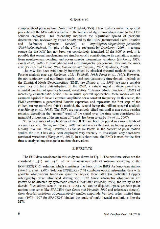
The EOP data considered in this study are shown in Fig. 1. The two time series are the

coordinates xt and yt of the instantaneous pole of rotation according to the EOP(IERS) C 01 solution, which constitutes the basis of the IERS for long-term studies (Vondrák et al., 1995). Solution EOP(IERS) C 01 combines optical astrometric data with geodetic observations based on space techniques; these latter (in particular, Doppler orbitography) were introduced starting with 1972. Since astrometric observations are known to be affected by systematic errors (Gross and Vondrák, 1999), the reality of the decadal fluctuations seen in the EOP(IERS) C 01 can be disputed. Space-geodetic polar motion time series like SPACE96 (see Gross and Vondrák, 1999 and references therein), show decadal variations of comparatively smaller amplitude, but their rather limited time span (19761997 for SPACE96) hinders the study of multi-decadal oscillations like the MW.

Empirical mode decomposition of long-term polar motion observations

Stud. Geophys. Geod., 59 (2015) iii

For the whole time period 1900present, the EOP(IERS) C 01 solution is given at 0.05-years time intervals. Since here we are concerned with rotational variations on time-scales of a few decades, we have applied to the original time series a low-pass Gaussian filter (see e.g. Young and Van Vliet, 1995) with full width at half maximum of 5 years. The Gaussian filter removes the high-frequency components of polar motion associated with the annual wobble and with the Chandler wobble (Höpfner, 2004) without

introducing high-frequency artifacts. The resulting smoothed time series sx t and

sy t are shown by thick curves in Fig. 1. Unfiltered time series would not be suitable

for the EMD analysis, since mode separation can be difficult when the signal contains components having adjacent periods (Chen and Feng, 2003; Kim and Oh, 2009), as it occurs for the annual and the Chandler wobbles. This mode mixing problem can be partly alleviated using a noise-assisted ensemble empirical mode decomposition (EEMD) (Wu and Huang, 2009; Torres et al., 2011). Since here we focus on multidecadal oscillations, mode mixing from high-frequency components of polar motion does not limit our analysis. However, below we have used EEMD in order to test the robustness of certain features of the MW.

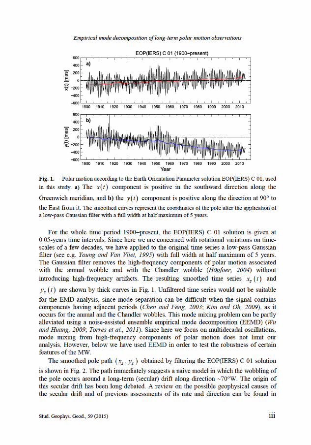
The smoothed pole path ,s sx y obtained by filtering the EOP(IERS) C 01 solution

is shown in Fig. 2. The path immediately suggests a naive model in which the wobbling of the pole occurs around a long-term (secular) drift along direction 70W. The origin of this secular drift has been long debated. A review on the possible geophysical causes of the secular drift and of previous assessments of its rate and direction can be found in

Fig. 1. Polar motion according to the Earth Orientation Parameter solution EOP(IERS) C 01, used

in this study. a) The xt component is positive in the southward direction along the

Greenwich meridian, and b) the yt component is positive along the direction at 90 to the East from it. The smoothed curves represent the coordinates of the pole after the application of a low-pass Gaussian filter with a full width at half maximum of 5 years.

G. Spada et al.

iv Stud. Geophys. Geod., 59 (2015)

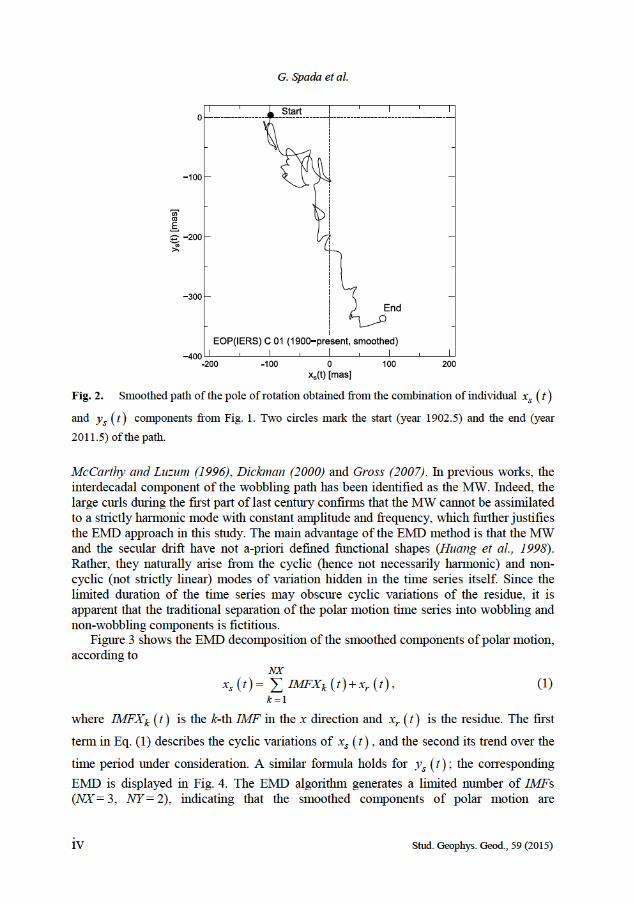
McCarthy and Luzum (1996), Dickman (2000) and Gross (2007). In previous works, the interdecadal component of the wobbling path has been identified as the MW. Indeed, the large curls during the first part of last century confirms that the MW cannot be assimilated to a strictly harmonic mode with constant amplitude and frequency, which further justifies the EMD approach in this study. The main advantage of the EMD method is that the MW and the secular drift have not a-priori defined functional shapes (Huang et al., 1998). Rather, they naturally arise from the cyclic (hence not necessarily harmonic) and non-cyclic (not strictly linear) modes of variation hidden in the time series itself. Since the limited duration of the time series may obscure cyclic variations of the residue, it is apparent that the traditional separation of the polar motion time series into wobbling and non-wobbling components is fictitious. Figure 3 shows the EMD decomposition of the smoothed components of polar motion,

according to

1

NX

s k rk

x t IMFX t x t

, (1)

where kIMFX t is the k-th IMF in the x direction and rx t is the residue. The first

term in Eq. (1) describes the cyclic variations of sx t, and the second its trend over the

time period under consideration. A similar formula holds for sy t; the corresponding

EMD is displayed in Fig. 4. The EMD algorithm generates a limited number of IMFs (NX = 3, NY = 2), indicating that the smoothed components of polar motion are

Fig. 2. Smoothed path of the pole of rotation obtained from the combination of individual sx t

and sy t components from Fig. 1. Two circles mark the start (year 1902.5) and the end (year

2011.5) of the path.

Empirical mode decomposition of long-term polar motion observations

Stud. Geophys. Geod., 59 (2015) v

characterized by a small number of characteristic time scales. Two of the modes found

(namely, 3IMFX and 2IMFY ) show a significant interdecadal variability and amplitudes

varying in the range of a few tens of mas. Thus, it is natural to identify these empirical modes (reminiscent of Markowitz’s “empirical term”), as those corresponding to the MW evidenced in previous studies. The IMFs with shorter periods describe sub-decadal wobblings, and could be interpreted as further components of the MW, or alternatively as oscillating features of the secular path of the pole.

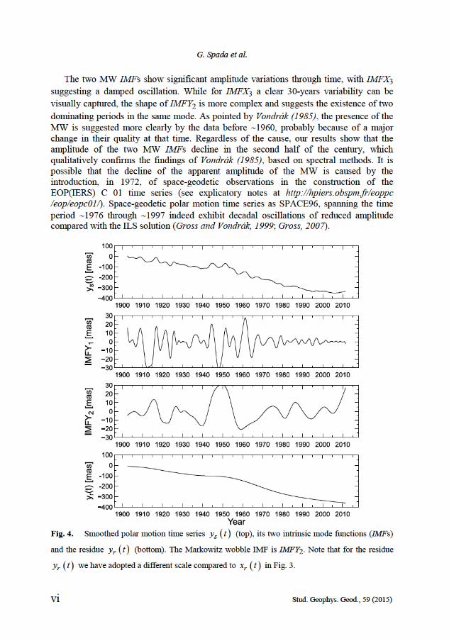
Fig. 3. Smoothed polar motion time series sx t (top), its three intrinsic mode functions (IMFs)

and the residue rx t (bottom). IMFX3, which corresponds to the Markowitz wobble IMF, is

shown by a thick curve.

G. Spada et al.

vi Stud. Geophys. Geod., 59 (2015)

The two MW IMFs show significant amplitude variations through time, with IMFX3

suggesting a damped oscillation. While for IMFX3 a clear 30-years variability can be

visually captured, the shape of IMFY2 is more complex and suggests the existence of two

dominating periods in the same mode. As pointed by Vondrák (1985), the presence of the MW is suggested more clearly by the data before 1960, probably because of a major change in their quality at that time. Regardless of the cause, our results show that the amplitude of the two MW IMFs decline in the second half of the century, which qualitatively confirms the findings of Vondrák (1985), based on spectral methods. It is possible that the decline of the apparent amplitude of the MW is caused by the introduction, in 1972, of space-geodetic observations in the construction of the EOP(IERS) C 01 time series (see explicatory notes at http://hpiers.obspm.fr/eoppc /eop/eopc01/). Space-geodetic polar motion time series as SPACE96, spanning the time period 1976 through 1997 indeed exhibit decadal oscillations of reduced amplitude compared with the ILS solution (Gross and Vondrák, 1999; Gross, 2007).

Fig. 4. Smoothed polar motion time series sy t (top), its two intrinsic mode functions (IMFs)

and the residue ry t (bottom). The Markowitz wobble IMF is IMFY2. Note that for the residue

ry t we have adopted a different scale compared to rx t in Fig. 3.

Empirical mode decomposition of long-term polar motion observations

Stud. Geophys. Geod., 59 (2015) vii

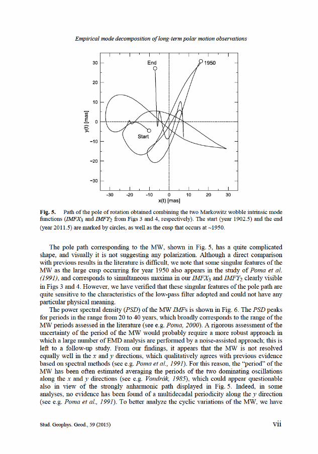
The pole path corresponding to the MW, shown in Fig. 5, has a quite complicated shape, and visually it is not suggesting any polarization. Although a direct comparison with previous results in the literature is difficult, we note that some singular features of the MW as the large cusp occurring for year 1950 also appears in the study of Poma et al. (1991), and corresponds to simultaneous maxima in our IMFX3 and IMFY2 clearly visible

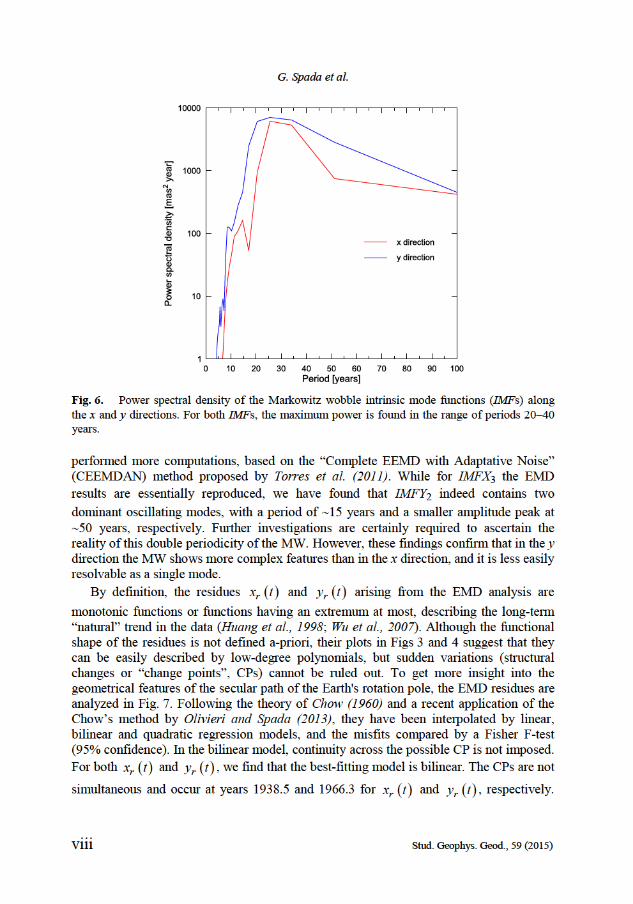
in Figs 3 and 4. However, we have verified that these singular features of the pole path are quite sensitive to the characteristics of the low-pass filter adopted and could not have any particular physical meaning. The power spectral density (PSD) of the MW IMFs is shown in Fig. 6. The PSD peaks

for periods in the range from 20 to 40 years, which broadly corresponds to the range of the MW periods assessed in the literature (see e.g. Poma, 2000). A rigorous assessment of the uncertainty of the period of the MW would probably require a more robust approach in which a large number of EMD analysis are performed by a noise-assisted approach; this is left to a follow-up study. From our findings, it appears that the MW is not resolved equally well in the x and y directions, which qualitatively agrees with previous evidence based on spectral methods (see e.g. Poma et al., 1991). For this reason, the “period” of the MW has been often estimated averaging the periods of the two dominating oscillations along the x and y directions (see e.g. Vondrák, 1985), which could appear questionable also in view of the strongly anharmonic path displayed in Fig. 5. Indeed, in some analyses, no evidence has been found of a multidecadal periodicity along the y direction (see e.g. Poma et al., 1991). To better analyze the cyclic variations of the MW, we have

Fig. 5. Path of the pole of rotation obtained combining the two Markowitz wobble intrinsic mode functions (IMFX3 and IMFY2 from Figs 3 and 4, respectively). The start (year 1902.5) and the end

(year 2011.5) are marked by circles, as well as the cusp that occurs at 1950.

G. Spada et al.

viii Stud. Geophys. Geod., 59 (2015)

performed more computations, based on the “Complete EEMD with Adaptative Noise” (CEEMDAN) method proposed by Torres et al. (2011). While for IMFX3 the EMD

results are essentially reproduced, we have found that IMFY2 indeed contains two

dominant oscillating modes, with a period of 15 years and a smaller amplitude peak at 50 years, respectively. Further investigations are certainly required to ascertain the reality of this double periodicity of the MW. However, these findings confirm that in the y direction the MW shows more complex features than in the x direction, and it is less easily resolvable as a single mode.

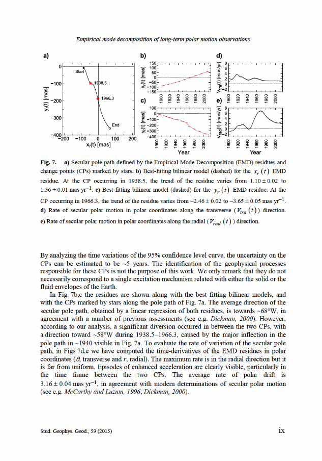
By definition, the residues rxt and ry t arising from the EMD analysis are

monotonic functions or functions having an extremum at most, describing the long-term “natural” trend in the data (Huang et al., 1998; Wu et al., 2007). Although the functional shape of the residues is not defined a-priori, their plots in Figs 3 and 4 suggest that they can be easily described by low-degree polynomials, but sudden variations (structural changes or “change points”, CPs) cannot be ruled out. To get more insight into the geometrical features of the secular path of the Earth's rotation pole, the EMD residues are analyzed in Fig. 7. Following the theory of Chow (1960) and a recent application of the Chow’s method by Olivieri and Spada (2013), they have been interpolated by linear, bilinear and quadratic regression models, and the misfits compared by a Fisher F-test (95% confidence). In the bilinear model, continuity across the possible CP is not imposed.

For both rxt and ry t, we find that the best-fitting model is bilinear. The CPs are not

simultaneous and occur at years 1938.5 and 1966.3 for rxt and ry t, respectively.

Fig. 6. Power spectral density of the Markowitz wobble intrinsic mode functions (IMFs) along the x and y directions. For both IMFs, the maximum power is found in the range of periods 2040 years.

Empirical mode decomposition of long-term polar motion observations

Stud. Geophys. Geod., 59 (2015) ix

By analyzing the time variations of the 95% confidence level curve, the uncertainty on the CPs can be estimated to be 5 years. The identification of the geophysical processes responsible for these CPs is not the purpose of this work. We only remark that they do not necessarily correspond to a single excitation mechanism related with either the solid or the fluid envelopes of the Earth. In Fig. 7b,c the residues are shown along with the best fitting bilinear models, and

with the CPs marked by stars along the pole path of Fig. 7a. The average direction of the secular pole path, obtained by a linear regression of both residues, is towards 68W, in agreement with a number of previous assessments (see e.g. Dickman, 2000). However, according to our analysis, a significant diversion occurred in between the two CPs, with a direction toward 58W during 1938.51966.3, caused by the major inflection in the pole path in 1940 visible in Fig. 7a. To evaluate the rate of variation of the secular pole path, in Figs 7d,e we have computed the time-derivatives of the EMD residues in polar coordinates (, transverse and r, radial). The maximum rate is in the radial direction but it is far from uniform. Episodes of enhanced acceleration are clearly visible, particularly in the time frame between the two CPs. The average rate of polar drift is

3.16 ± 0.04 mas yr1, in agreement with modern determinations of secular polar motion (see e.g. McCarthy and Luzum, 1996; Dickman, 2000).

Fig. 7. a) Secular pole path defined by the Empirical Mode Decomposition (EMD) residues and

change points (CPs) marked by stars. b) Best-fitting bilinear model (dashed) for the rx t EMD

residue. At the CP occurring in 1938.5, the trend of the residue varies from 1.10 ± 0.02 to

1.56 ± 0.01 mas yr1. c) Best-fitting bilinear model (dashed) for the ry t EMD residue. At the

CP occurring in 1966.3, the trend of the residue varies from 2.46 ± 0.02 to 3.65 ± 0.05 mas yr1.

d) Rate of secular polar motion in polar coordinates along the transverse ( traV t ) direction.

e) Rate of secular polar motion in polar coordinates along the radial ( radV t ) direction.

G. Spada et al.

x Stud. Geophys. Geod., 59 (2015)

3. CONCLUSIONS

A straightforward application of the EMD method to polar motion data confirms the existence of a variable wobbling of the Earth’s pole of rotation in astrometric time series, which we identify with the “empirical term” discovered by Markowitz (1960). Although both the amplitude and the period of the MW are subject to significant fluctuations, our analysis indicates that the first attains a maximum value of 25 mas while the second is estimated in the range of 20 to 40 years, in agreement with previous studies. Our analysis is based upon the assumption that the amplitude of systematic errors contained in the astrometric data is not large enough to disrupt the significance of the decadal oscillations we have found. Based on the results of Gross and Vondrák (1999) and Gross (2007), the decadal variations shown by space-geodetic have a smaller amplitude than those detected in the ILS series. Hence, following Gross (2007), the decadal variations we have evidenced could be considered as a possible upper bound of the effective size of the decadal variations. Since the EMD approach is totally independent from the traditional spectral methods

historically adopted to analyze polar motion data, our findings bring a strong evidence in support to the existence of the MW. However, this can be hardly described as an harmonic oscillation. Here, the secular polar motion is identified with the EMD residue, i.e. the non-cyclic component of the polar motion path. The time-averaged rate and direction of secular polar motion are found to be in in good agreement with previous analyses. An investigation of the geophysical causes of the abrupt variations (change points) that we have detected along the secular path of the pole would probably merit a follow-up study. Acknowledgments: We have benefited from very insightful comments from Richard Gross. The

figures have been drawn using GMT (Wessel and Smith, 1998). Some of the computations have been also been performed by GMT tools. The EMD analysis has been carried out using program EMD, made available by Lionel Loudet from http://sidstation.loudet.org/emd-en.xhtml and CEEMDAN, developed by Maria Eugenia Torres and available from http://bioingenieria.edu.ar/grupos/ldnlys/metorres/re_inter.htm. The EOP(IERS) C 01 time series is obtained from http://hpiers.obspm.fr/eoppc/eop/eopc01/ (file eopc01.1900-now, downloaded on July 16, 2014). Funded by a DiSBeF (Dipartimento di Scienze di Base e Fondamenti, Urbino University) research grant No. CUP H31J13000160001.

References

Chen Y. and Feng M.Q., 2003. A technique to improve the empirical mode decomposition in the Hilbert-Huang transform. Earthq. Eng. Eng. Vib., 2, 7585.

Chow G.C., 1960. Tests of equality between sets of coefficients in two linear regressions. Econometrica, 28, 591605.

Dickman S., 1981. Investigation of controversial polar motion features using homogeneous International Latitude Service data. J. Geophys. Res., 86(B6), 49044912.

Dickman S., 1983. The rotation of the ocean - solid Earth system. J. Geophys. Res., 88(B8), 63736394.

Empirical mode decomposition of long-term polar motion observations

Stud. Geophys. Geod., 59 (2015) xi

Dickman S., 2000. Tectonic and cryospheric excitation of the Chandler Wobble and a brief review of the secular motion of Earth’s rotation pole. In: Dick S., McCarthy D. and Luzum B. (Eds), Polar Motion: Historical and Scientific Problems, IAU Colloquium 178. Vol. 208, 421436.

Dumberry M., 2008. Gravitational torque on the inner core and decadal polar motion. Geophys. J. Int., 172, 903920.

Dumberry M. and Bloxham J., 2002. Inner core tilt and polar motion. Geophys. J. Int., 151, 377392.

Gross R.S., 1990. The secular drift of the rotation pole. In: Boucher C. and Wilkins G.A. (Eds), Earth Rotation and Coordinate Reference Frames. International Association of Geodesy Symposia 105. Springer-Verlag, Heidelberg, Germany, 146–153.

Gross R.S., 2007. Earth rotation variations - long period. In: Schubert G. (Ed.), Treatise on Geophysics 3, 239294. Elsevier, Amsterdam, The Netherlands, ISBN: 9780444527486, DOI: 10.1016/B978-044452748-6.00057-2.

Gross R.S. and Vondrák J., 1999. Astrometric and space-geodetic observations of polar wander. Geophys. Res. Lett., 26, 20852088.

Höpfner J., 2004. Low-frequency variations, Chandler and annual wobbles of polar motion as observed over one century. Surv. Geophys., 25, 154.

Huang N.E. and Shen S.S. (Eds), 2005. Hilbert-Huang Transform and its Aapplications. World Scientific, Singapore. ISBN: 978-981-256-376-7 (hardcover), 978-981-4480-06-2 (ebook).

Huang N.E., Shen Z., Long S.R.,Wu M.C., Shih H.H., Zheng Q., Yen N.-C., Tung C.C. and Liu H.H., 1998. The empirical mode decomposition and the Hilbert spectrum for nonlinear and non-stationary time series analysis. Proc. R. Soc. London A, 454, 903995.

Huang N.E. and Wu Z., 2008. A review on Hilbert-Huang transform: Method and its applications to geophysical studies. Rev. Geophys., 46, RG2006, DOI: 10.1029/2007RG000228.

Kim D. and Oh H.-S., 2009. EMD: a package for empirical mode decomposition and Hilbert spectrum. R Journal, 1, 4046.

Lambeck K., 2005. The Earth’s Variable Rotation: Geophysical Causes and Consequences. Cambridge University Press, Cambridge, U.K.

Markowitz W., 1960. Latitude and longitude, and the secular motion of the pole. In: Runcorn S.K. (Ed.), Methods and Techniques in Geophysics. Interscience Publishers, London, U.K., 325361.

McCarthy D.D. and Luzum B.J., 1996. Path of the mean rotational pole from 1899 to 1994. Geophys. J. Int., 125, 623629.

Olivieri M. and Spada G., 2013. Intermittent sea–level acceleration. Global Planet. Change, 109, 6472.

Poma A., 2000. The Markowitz wobble. In: Dick S., McCarthy D. and Luzum B. (Eds), Polar Motion: Historical and Scientific Problems, IAU Colloquium 178. Vol. 208, 351354.

Poma A., Proverbio E. and Uras S., 1991. Decade fluctuations in the Earth’s rate of rotation and long–term librations in polar motion. Il Nuovo Cimento, C14, 119125.

Ponte R., Rajamony J. and Gregory J., 2002. Ocean angular momentum signals in a climate model and implications for Earth rotation. Clim. Dyn., 19, 181190.

G. Spada et al.

xii Stud. Geophys. Geod., 59 (2015)

Torres M.E., Colominas M.A., Schlotthauer G. and Flandrin P., 2011. A complete ensemble empirical mode decomposition with adaptive noise. In: 2011 IEEE International Conference on Acoustics, Speech and Signal Processing (ICASSP). The Institute of Electrical and Electronics Engineers, Piscataway, NJ, 41444147, DOI: 10.1109/ICASSP.2011.5947265.

Vicente R. and Currie R., 1976. Maximum entropy spectrum of long-period polar motion. Geophys. J. Int., 46, 6773.

Vondrák J., 1985. Long-period behaviour of polar motion between 1900.0 and 1984.0. Ann. Geophys., 3, 351356.

Vondrák J., Ron C., Pešek I. and Čepek A., 1995. New global solution of earth orientation parameters from optical astrometry in 19001990. Astron. Astrophys., 297, 899906.

Wang X.H., Wang Q.J. and Liu J., 2012. Application of empirical mode decomposition in the ultra short-term prediction of polar motion. Acta Astronomica Sinica, 53, 519526.

Wessel P. and Smith W.H.F., 1998. New, improved version of Generic Mapping Tools released. EOS Trans. AGU, 79, 579.

Wu Z. and Huang N.E., 2009. Ensemble empirical mode decomposition: a noise-assisted data analysis method. Adv. Adapt. Data Anal., 1, 141.

Wu Z., Huang N.E., Long S.R. and Peng C.-K., 2007. On the trend, detrending, and variability of nonlinear and nonstationary time series. Proc. Nat. Acad. Sci., 104, 1488914894.

Young I.T. and Van Vliet L.J., 1995. Recursive implementation of the Gaussian filter. Signal Process., 44, 139151.