RESEARCH SEMINAR IN INTERNATIONAL ECONOMICS

Gerald R. Ford School of Public Policy The University of Michigan

Ann Arbor, Michigan 48109-1220

Discussion Paper No. 505

Empirical Analysis of Barriers to International Services Transactions

and the Consequences of Liberalization

Alan V. Deardorff and Robert M. Stern University of Michigan

January 2, 2004

Recent RSIE Discussion Papers are available on the World Wide Web at: http://www.fordschool.umich.edu/rsie/workingpapers/wp.html

2

TRADE IN SERVICES AND INTERNATIONAL TRADE AGREEMENTS: THE DEVELOPMENT DIMENSION

A World Bank Course

Module 2: Empirical Analysis of Barriers to International Services Transactions and the Consequences of Liberalization

Alan V. Deardorff and Robert M. Stern

University of Michigan Revised January 2, 2004 Address correspondence to: Robert M. Stern Department of Economics University of Michigan Ann Arbor, MI 48109-1220 Tel. 734-764-2373 FAX 810-277-4102 E-Mail rmstern@umich.edu URL http://www.umich.edu/~rmstern/

Empirical Analysis of Barriers to International Services Transactions and the Consequences of Liberalization

Alan V. Deardorff and Robert M. Stern

University of Michigan

Executive Summary

This module provides an overview of the methods that can be used to identify and quantify barriers to international trade in services. Trade in services is customarily classified into four “modes of supply”: Mode 1 – services that are traded internationally across borders; Mode 2 – services that require the consumer to be in the location of the producer; Mode 3 – services that require commercial presence in the form of foreign direct investment; and Mode 4 – services that require the temporary cross-border movement of workers. Barriers to any of these forms of trade typically take the form of regulations that either restrict supply or make it more costly. In either case, the economic impact of such a barrier can in principle be quantified as a “tariff equivalent,” defined as the percentage tax on foreign suppliers that would have the same effect on the domestic market for the service as is caused by the barrier.

Barriers to trade in services are extremely diverse, making it difficult to classify them in any simple yet detailed way. Broadly, they may be separated on the one hand into those that restrict entry of firms versus those that affect firms’ operations, and on the other hand into those that discriminate against foreign service providers versus those that do not. Within these broad categories, barriers have been classified much more finely in terms of characteristics that are appropriate to particular service industries.

Measurement of service barriers can be either direct or indirect. Direct measurement involves documenting barriers that are known to exist, either by extracting information about them from government documents or by questioning those market participants who confront them. Ideally, both of these methods should be based on detailed knowledge of the industries involved, since services differ greatly among themselves in the kinds of regulations that apply to them and in the rationales and effects of these regulations.

Indirect measurement attempts to infer the presence of barriers from their market effects, much as nontariff barriers on trade in goods are often inferred from price differences across borders. Unfortunately, most services do not cross a border in this way, and even those that do are often differentiated sufficiently that comparable prices do not exist inside and outside of countries. Thus indirect measurement has to be even more indirect, drawing heavily on theoretical models of activity in the absence of barriers.

We illustrate these various approaches by citing in some detail a number of studies that have been carried out, some for broad categories of service trade and others for particular sectors. We also, in an appendix, summarize a much larger number of studies. Procedures differ somewhat across studies, but most employ one or more of the following steps:

ii

• Collect the details of regulations and other policies affecting service firms in the countries and/or sectors being examined. Ideally, this information should be collected by systematic surveys of governments and/or firms. However, it may also be possible to infer it less directly from documents prepared for other purposes.

• For each type of regulation or policy, define degrees of restrictiveness and assign scores to each.

• Construct an index of restrictiveness by: weighting the above scores based on subjective judgments; using a statistical methodology; or designing proxy measures.

• Convert these indices of restrictiveness into a set of tariff equivalents by one or more of the following methods.

o Assign judgmental tariff-equivalent values to each component of the index.

o Use data on prices and their determinants in a regression model to estimate the effect on prices.

o Use data on quantities produced or traded in a regression model to estimates the effect on quantities, and convert to tariff equivalents.

• Use the above measures as inputs into a model of production and trade in order to ascertain the economic effects of the presence of changes in the services barriers involved.

Empirical Analysis of Barriers to International Services

Transactions and the Consequences of Liberalization

Alan V. Deardorff and Robert M. Stern University of Michigan

I. Introduction

Issues to be Addressed: • Modes of supply of services • Direct versus indirect measurement of barriers • Overview of the module

Barriers to trade interfere with the ability of firms from one country to compete with firms from

another. This is true of trade in goods, where a tariff or nontariff barrier (NTB) typically drives a wedge

between the price of the good on the world market and its domestic price. This wedge, or “tariff

equivalent,” provides a convenient and often observable measurement of the size of the impediment. In

the case of services, however, no such simple measurement is often observable. It remains true, though,

that the concept of a tariff equivalent – now thought of as the equivalent tax on foreign suppliers in their

competition with domestic suppliers – is a useful way of quantifying a barrier to trade even though it may

be much harder to observe. Both the role of barriers to trade in services and the possible meaning of a

tariff equivalent can be better understood in the context of each of the standard four “modes of supply”

that arise for traded services and are shown in Table 1 for 1997. The four modes of supply are:

• Mode 1 – services that are traded internationally across borders

• Mode 2 – services that require the consumer to be in the location of the producer

• Mode 3 – services that require commercial presence in the form of foreign direct investment

• Mode 4 – services that require the temporary cross-border movement of workers

To clarify further, Mode 1 refers to “separated” services such as telecommunications, which are

traded internationally across borders in a manner similar to cross-border trade in goods. Here, foreign

suppliers of a service provide it to domestic buyers through international means of communication and

2

perhaps transportation, with a unit of the service itself often unobservable as it crosses national borders.

A French telecoms company, for example, may provide telephone services to a customer in Mexico, in

competition with a Mexican-based provider. A trade barrier in this case might consist of Mexican

restrictions on the French firm’s access to phone lines in Mexico, discriminatory taxes on its operations,

or regulations on the ways that Mexican consumers are allowed to access the foreign firm’s services. A

tariff equivalent of all such impediments would be defined as the tax on the French firm’s operations in

Mexico that, if it replaced all other impediments, would cause it to operate at the same level and have the

same effects on the domestic telecoms providers and consumers within Mexico. As in the case of traded

goods, a single tariff equivalent may not capture all of these effects simultaneously, especially if

competition is imperfect. And even with perfect competition, such a tariff equivalent is unlikely to be

observable as a simple price difference. There is no world price of Mexican telephone services, for

example, with which to compare what Mexican firms are charging, since the nature and cost of a service

depend in part on the location of the consumer. Nonetheless, a tariff equivalent is a conceptually useful

way of quantifying barriers to trade in services as well as goods, and many studies have sought to express

their results in this form.

Mode 2 of services trade refers to services that require the consumer to be in the location of the

producer, as in the cases of tourism and education. Here again, the service provided is likely to be

differentiated by the location or identity of the provider, so that a world price of the service may not be

meaningful. It would be meaningless, for example, to try to compare the “world price” of a visit to the

Taj Mahal or an MBA degree from the Wharton School with the prices of these services within, say,

Brazil. But it remains the case that Brazilian restrictions on their citizens’ travel to India or the U.S. to

consume these services will alter the markets for other tourist attractions and educational institutions

within Brazil. Such restrictions again can in principle be quantified as equivalent to a tax on Brazilians’

visits abroad for these purposes.

Mode 3 of international services provision is arguably the most general and the most important:

provision through a commercial presence that is the result of foreign direct investment (FDI). Almost any

3

service can be provided by firms from one country to consumers in another if the firms are allowed to

establish a physical presence there. This is true even of tourism – think of Euro-Disney. In this case there

may well be a foreign price with which one could easily compare, but the comparison is unlikely to be

meaningful. It would be a mistake to infer a trade barrier from the higher price of admission to Euro-

Disney in Paris as compared to Florida, or the absence of a trade barrier from the lower price of a

McDonald’s hamburger in Argentina than in New York. In all such cases, prices depend on local costs of

labor and raw materials as much as they do on trade barriers. However, and once again, foreign service

providers may well face impediments, both to their establishment and to their ongoing operations, the

effects of which would be similar to a tax if only we could infer what it is.

The final mode of supply, Mode 4, refers to the temporary cross-border movement of workers.

Examples are the movement of computer programmers, engineers, management personnel, and lesser

skilled construction workers who are granted temporary visas to work in a host country. Most movement

that is actually permitted consists of workers within industries that produce traded goods or that produce

services that are primarily thought of as traded through other modes. Thus we do not think of many

industries as producing services that are primarily traded through Mode 4. On the other hand, labor itself

is a service that could be traded in this way, and occasionally it has been, in the form of guest-worker

programs and the like. The fact that Mode 4 service-provision figures appear to be relatively small in the

data on services trade in Table 1 is therefore symptomatic of the very high barriers that exist for Mode 4,

except within industries where it facilitates other kinds of trade. Mode 4 is the one mode in which the

tariff equivalent of barriers could most easily be measured, as simply the differences across countries in

the real wages of particular kinds of labor.

For all of the modes, then, one objective of empirical measurement is to deduce some sort of

tariff equivalent of the barrier to trade in particular services. Since direct price comparisons seldom serve

that purpose, however, researchers have pursued other means of inferring the presence and size of barriers

to trade. Some of these methods have been quite direct: they simply ask governments or participants in

markets what barriers they impose or face. The answers are usually only qualitative, indicating the

4

presence or absence of a particular type of barrier, but not its quantitative size or effect. Such qualitative

information takes on a quantitative dimension, however, when it is tabulated by sector, perhaps with

subjective weights to indicate severity. The result is a set of “frequency measures” of barriers to trade,

recording what the barriers are and where, and perhaps also the fraction of trade within a sector or country

that is subject to them. Frequency measures do not directly imply anything like the tariff equivalents of

trade barriers, but in order to use them for quantitative analysis, analysts have often converted them to

that form in rather ad hoc ways that we will indicate below.

Other, more indirect, measurements of trade barriers in service industries have also been used,

alone or in combination with frequency measures. These may be divided into two types: measurements

that use information about prices and/or costs; and measurements that observe quantities of trade or

production and attempt to infer how trade barriers have affected these quantities. In both cases, as we will

discuss, if one can also measure or assume an appropriate elasticity reflecting the response of quantity to

price, a measured effect on either can be translated into an effect on the other. Thus both price and

quantity measurements are also often converted into, and reported as, tariff equivalents.

In what follows, we begin in Section II with a conceptual framework for understanding

international services transactions and the barriers that may affect them. We then turn in Section III to a

discussion of the characteristics of services barriers, and we provide some examples of barriers for the

banking sector and for foreign direct investment in services sectors. This is followed in Section IV with a

discussion of methods of measurement of services barriers, including frequency measures and indexes of

restrictiveness, price-effect and quantity-effect measurements, gravity-model estimates, and financial-

based measurements. In each case, we provide information and examples of how the measurements are

constructed and an evaluation of their merits and limitations. We also provide in Appendix A brief

summaries of studies that have used these methods. In Section V, we consider how the various

measurements can be used in assessing the economic consequences of the liberalization of services

barriers. Since this module is designed for instructional purposes, we conclude in Section VI with a

presentation of guideline principles and recommended procedures for measuring services barriers and

5

assessing the consequences of their liberalization. Finally, we include two appendices, one containing

discussion of selected technical issues and summaries of literature pertinent to methods of measurement

of services barriers, and the second containing study questions and exercises for instructional use.

II. Conceptual Framework

Issues to be Addressed: • Service market equilibrium • Differentiated services • Imperfect competition

In this section, we use demand-and-supply analysis to show how the introduction of a services

barrier will affect the domestic price of a service, the quantity demanded, and the quantity supplied by

domestic and foreign firms. We show, using diagrammatic analysis, how the service barrier can be

measured as a tariff equivalent. Three cases are presented:

• Figure 1 -- domestic and foreign firms are highly competitive and their services are highly substitutable.

• Figure 2 -- the services of the domestic and foreign firms are not readily substitutable and have

distinctive prices.

• Figure 3 -- there is a single domestic firm with monopoly power and the entry of foreign firms is restricted.

The effects of a service barrier, and thus the tariff equivalent, in these various cases will depend on the

competitiveness of domestic and foreign firms and the degree of substitution between the services that

they provide.

Figure 1 illustrates the functioning of a domestic market for a service when there are domestic

and foreign suppliers present. It is assumed here that the suppliers are highly competitive and that their

services are readily substitutable. Other cases will be considered below. The foreign suppliers may be

serving the domestic market through any of the four modes of supply already discussed, although the

degree of substitution between the foreign and domestic services may vary for the different modes.

6

The horizontal axis in Figure 1 measures the quantity of the service supplied to and demanded by

domestic purchasers. This could include amounts purchased abroad, as in the case of Mode 2, which are

nonetheless regarded here as competing with domestic supplies. The demand schedule for the service is

downward sloping with respect to the price, P, which is the same for all suppliers. The supply schedules

for the two sets of suppliers, domestic and foreign, are upward sloping and shown by SD for domestic

firms and SF for foreign firms.1 In the absence of any impediments to trade, the relevant total supply

schedule in this market is the horizontal sum, labeled SD+SF. Price is determined where the total supply

schedule intersects the demand schedule at P0, with the quantity Q0 divided between domestic firms, 0DQ ,

and foreign firms, 0FQ .

Let us suppose now that a barrier is introduced that inhibits the ability of the foreign firms to

serve this market. This may raise foreign firms’ costs, shifting their supply schedule upward, or it may

reduce or constrain the quantity that they supply, shifting the schedule to the left. Either way, SF is shifted

up and to the left, as is the total supply schedule, SD+SF, to the positions shown as SF’ and SD+SF’. The

effect is to raise the price of the service to P1, reduce the total quantity purchased, and increase the

quantity sold by domestic firms. Sales by the foreign firms fall from 0FQ to 1

FQ , which is the decline in

imports of the service due to the barrier.

The tariff equivalent of this barrier may be defined as the ad valorem tax on foreign service

providers that would have caused the same effects as this barrier. Such a tax, by increasing the cost of

sales by foreign firms, would cause their supply schedule to shift up by the amount of the tax. Therefore,

a tax that shifts SF up so as to pass through point A is the tariff equivalent. That is, the tariff equivalent is

the percentage by which point A lies above point B. What should be noted in the case of Figure 1 is that

the tariff equivalent is not measurable from any observable price or price change. That is, the increase in

the price of the service on the domestic market is considerably smaller than the tariff equivalent of the

barrier that caused it. 1 Domestic supply is shown as further to the right (larger quantity for given price) than foreign supply, but this is not needed for any of the implications of the analysis.

7

There is, however, one special case in which the tariff equivalent would equal the price change.

This occurs when the foreign supply schedule is horizontal (i.e., infinitely elastic) at some price P0 so that

the effect of the barrier is to raise foreign firms’ cost to P1. Then the two foreign supply schedules are

horizontal at these prices, and the tariff equivalent would be just the amount by which they are shifted

upward. To the extent that empirical measurements of tariff equivalents are based on observed prices, a

horizontal foreign supply schedule will represent a special case that may exist for a small country that

faces a given world price for the service.

Figure 2 shows a case in which the services provided by domestic and foreign firms are not

readily substitutable and can therefore have different prices. In this case we must consider markets for the

two services separately, as is done in the two panels of Figure 2, and we must also allow for the two

services being imperfect substitutes. This is done by having each of the two demand schedules depend on

the price in the other market, as indicated. Once again, the figure shows supply and demand schedules,

quantities, and prices without any trade barrier with superscript 0, and those in the presence of a trade

barrier with superscript 1. The introduction of a barrier shifts the foreign supply schedule to the left and

up, as before, to 1FS and leads to higher prices in both markets, 1

FP and 1DP , which now cause both

demand schedules to shift somewhat to the right. As in the case of Figure 1, with close substitution of the

services, the domestic quantity supplied increases while the foreign quantity supplied declines. And here

again, the tariff equivalent can be observed in the figure as the percentage by which 1FS lies above 0

FS ,

that is, the percentage by which point A is above point B.

So far we have assumed that markets are highly competitive. But this is clearly inappropriate in

many service markets where an incumbent domestic firm may have a monopoly or only a very limited

number of competitors. In such markets, a barrier to service trade may be a limit on entry by new firms

that, though not explicitly discriminatory, favors the domestic incumbent firm and implicitly limits trade

more than domestic supply. We therefore now consider, in Figure 3, the case in which there is a single

domestic incumbent firm together with competing foreign suppliers. If there is unimpeded entry of firms,

8

the market price will be P0. In this case, the single domestic firm whose costs are increasing along MC

will produce 0DQ . Total sales are Q0, and the foreign firms will sell 0

FQ = Q0 − 0DQ in the domestic

market. Let us now suppose that a barrier is introduced that raises the cost of the foreign firms when they

sell in the domestic market. This would cause the domestic firm’s sales to rise along MC and foreign

sales to decline. If the foreign cost rises above Pa (the intersection of domestic MC and demand),

however, then foreign sales will fall to zero. The domestic firm can thus charge a price that just barely

undercuts the foreign cost, so that the domestic firm will be able to monopolize the market. The tariff

equivalent of the barrier in the case of Figure 3 is therefore the amount by which it increases foreign cost,

up to the limit of Pm−P0. However, if the foreign supply schedule were instead upward sloping rather

than horizontal, then both the analysis and the identification of the tariff equivalent would be accordingly

more difficult to measure. But the general conclusion is that the tariff equivalent of an entry restriction

will be measured by the excess of the monopoly price over the competitive price that would have

obtained if both trade and entry were free.

Figures 1-3 clearly do not exhaust all of the possible cases. The real world is bound to involve

further mixtures of imperfect substitution between the products of domestic and foreign services firms

and the degree of competition between these firms that have not been considered here. Also, many

service industries have numerous special features, both in the ways that they operate and in their

amenability to measurement, and simple theoretical models do not take these factors into account.

Empirical work is therefore essential to address the measurement of the various services barriers that

impede international services transactions. In what follows, we review and summarize many of the

studies that have been done.

9

III. Characteristics of Services Barriers

Issues to be Addressed: • Broad classifications of service barriers • Detailed classifications: example • Barriers on foreign direct investment • Legitimate versus illegitimate regulations

As noted by Hoekman and Primo Braga (1997, p. 288), border measures such as tariffs are

generally difficult to apply to services because customs agents cannot readily observe services as they

cross the border. It is also the case, as discussed above, that many services are provided in the country of

consumption rather than cross-border. Typically, therefore, services restrictions are designed in the form

of government regulations applied to the different modes of services transactions. Thus, for example,

regulations may affect the entry and operations of both domestic and foreign suppliers of services and in

turn increase the price or the cost of the services involved. Services barriers are therefore more akin to

NTBs than to tariffs, and their impact will depend on how the government regulation is designed and

administered.

These regulations can take many forms, and are usually specific to the type of service being

regulated. Therefore, since services themselves are so diverse, services barriers are also diverse, making

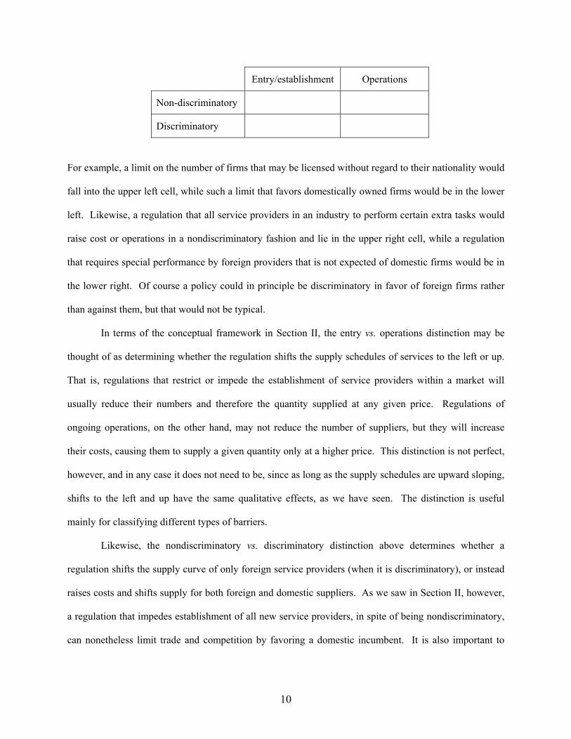
them somewhat difficult to classify in general terms. There are, however, two distinctions that that tend

to apply across many types of services and service barriers: regulations that apply to entry or

establishment of firms versus their operations; and regulations that are nondiscriminatory versus

discriminatory.2 That is, most barriers to trade in services can be placed in one of the four cells of the

following simple 2×2 classification:

2These distinctions are suggested by the Australian Productivity Commission, whose website can be consulted

for more details, (www.pc.gov.au/research/memoranda/servicesrestriction/index.html). See also Hoekman and Braga (1997, p. 288), who classify and provide examples of services barriers as follows: (1) quotas, local content, and prohibitions; (2) price-based instruments; (3) standards, licensing, and procurement; and (4) discriminatory access to distribution networks.

10

Entry/establishment Operations

Non-discriminatory

Discriminatory

For example, a limit on the number of firms that may be licensed without regard to their nationality would

fall into the upper left cell, while such a limit that favors domestically owned firms would be in the lower

left. Likewise, a regulation that all service providers in an industry to perform certain extra tasks would

raise cost or operations in a nondiscriminatory fashion and lie in the upper right cell, while a regulation

that requires special performance by foreign providers that is not expected of domestic firms would be in

the lower right. Of course a policy could in principle be discriminatory in favor of foreign firms rather

than against them, but that would not be typical.

In terms of the conceptual framework in Section II, the entry vs. operations distinction may be

thought of as determining whether the regulation shifts the supply schedules of services to the left or up.

That is, regulations that restrict or impede the establishment of service providers within a market will

usually reduce their numbers and therefore the quantity supplied at any given price. Regulations of

ongoing operations, on the other hand, may not reduce the number of suppliers, but they will increase

their costs, causing them to supply a given quantity only at a higher price. This distinction is not perfect,

however, and in any case it does not need to be, since as long as the supply schedules are upward sloping,

shifts to the left and up have the same qualitative effects, as we have seen. The distinction is useful

mainly for classifying different types of barriers.

Likewise, the nondiscriminatory vs. discriminatory distinction above determines whether a

regulation shifts the supply curve of only foreign service providers (when it is discriminatory), or instead

raises costs and shifts supply for both foreign and domestic suppliers. As we saw in Section II, however,

a regulation that impedes establishment of all new service providers, in spite of being nondiscriminatory,

can nonetheless limit trade and competition by favoring a domestic incumbent. It is also important to

11

note that some regulations may be designed to achieve certain social objectives, such as health and safety

or environmental requirements, and may not be protectionist in intent.

Of course, actual regulations differ greatly across service industries and are often based on

characteristics of the particular service being provided. Thus, within each cell of the table above we may

think of additional distinctions being made, usually distinctions that are peculiar to the service sector

under consideration.

To illustrate, we use the case of banking services based on a study by McGuire and Schuele

(2000) done under the auspices of the Australian Productivity Commission. Table 2 lists groupings of

restrictions that apply especially to Modes 3 and 4 of international banking services transactions. These

restrictions relate to commercial presence and “other restrictions” applied to banking services, together

with a brief indication of what these restrictions represent and how an index of them has been

constructed.3 As McGuire and Schuele note (p. 206): “The commercial presence grouping covers

restrictions on licensing, direct investment, joint venture arrangements, and the movement of people. The

‘other restrictions’ grouping covers restrictions on raising funds, lending funds, providing other lines of

business (insurance and securities services), expanding banking outlets, the composition of the board of

directors and the temporary movement of people.” Thus the top half of Table 2 corresponds roughly to

regulations of entry/establishment in the small table above, while the bottom half corresponds to roughly

to regulations of operations. For each type of restriction, separate columns also indicate whether they

apply to foreign and domestic firms, hence being discriminatory if they apply only to the former. An

indication of the restrictiveness of these regulations is also provided in Table 2 and will be discussed

below.

Just as different sub-classifications may be needed for different types of services, so too may the

appropriate classification depend on the purpose for which the classification will be used. This point is

made especially by Hardin and Holmes (1997) in their discussion of barriers affecting FDI (Mode 3).

3 See the Productivity Commission website for detailed listings by country of the categories of domestic and

foreign restrictions on establishment and ongoing operations for some selected services sectors, including: accountancy, architectural, and engineering services; banking; distribution; and maritime services.

12

Focusing, in effect, on the lower left cell of our table above – the establishment of a commercial presence

in many sectors in host countries – they define (p. 24) an FDI barrier as “…any government policy

measure which distorts decisions about where to invest and in what form.” In considering ways of

classifying such FDI barriers, they note (pp. 33-34):4

“The appropriate classification system may vary, depending on the purpose of the exercise. For example, if the purpose is to check and monitor compliance with some policy commitment, then the categories should reflect the key element of the commitment…. If the primary interest is instead the resource allocation implications of the barriers, some additional or different information may be useful. Barriers to FDI may distort international patterns and modes of…trade. They may also distort allocation of capital between different economies, between foreign and domestic investment, between different sectors, and between portfolio and direct investment. …the classification system…should highlight the key characteristics of the barriers that will determine their size and impact. Market access and national treatment are…relevant categories from a resource allocation perspective. …national treatment is generally taken to refer to measures affecting firms after establishment. A…way to classify barriers is therefore…according to what aspect of the investment they most affect: establishment, ownership and control; or operations. In addition…, some further information may be useful…on distinctions…between direct versus indirect restrictions on foreign controlled firms; and rules versus case-by-case decisions.”5

The main types of FDI barriers that have been identified by UNCTAD (1996) are noted in Table

3, which divides barriers into three groups, the first of which concerns entry and the last operations. The

middle group – ownership and control restrictions – illustrates the weakness of any simple classification

system since it seems to include elements of both. Further information on the barriers most commonly

used to restrict FDI especially in the APEC economies is provided in Hardin and Holmes (1997, esp. pp.

37-40 and 45-55). As they note (p. 40), some common characteristics appear to be:6

“application of some form of screening or registration process involving various degrees of burden for the foreign investor; restrictions on the level or share of foreign ownership, particularly in some service sectors, and often in the context of privatisations; widespread use of case-by-case judgments, often based on national interest criteria; widespread use

4 See also Holmes and Hardin (2000). 5 Direct restrictions include limitations on the total size or share of investment in a sector and requirements on

inputs used (e.g., local content). Indirect restrictions include net benefit or national interest criteria and limitations on membership of company boards. The distinction between rules and case-by-case decisions relates to issues of clarity in specification and transparency as compared to the exercise of administrative discretion.

6 Hardin and Holmes (pp. 40-43) also provide information on investment incentives, which are widely used and for the most part are not subject to multilateral disciplines.

13

of restrictions on ownership and control (e.g., restrictions on board membership), particularly in sectors such as telecommunications, broadcasting, banking; and relatively limited use of performance requirements on input controls in services sectors.”

It is evident from the foregoing discussion that services barriers exist in a variety of

forms, depending on the types of services involved, the country imposing the barriers, and the

sectors to which the barriers are applied. To help further the understanding of the different

services barriers, it would be useful accordingly to organize the available information by country

and sector, according to the four modes of international services transactions and whether or not

they are protectionist in intent. As already noted, these modes cover: cross-border services

(Mode 1); consumption abroad (Mode 2); FDI (Mode 3); and the temporary movement of

workers (Mode 4). Using this information, the next and difficult step will be to devise methods

of measurement of the various barriers and to integrate these measures within a framework

designed to assess their economic effects.

It should be emphasized, finally, that not all regulations of services should be viewed as

protectionist, even when they do serve to reduce service imports. Many regulations serve

legitimate purposes, such as protecting health and safety or preventing fraud and other

misconduct. Such a regulation, if applied in a nondiscriminatory manner, is not protectionist and

should not be viewed as a barrier to service trade, even though it may maintain a higher standard

than prevails abroad and thus reduce imports compared to what they would be without the

regulation. On the other hand, nondiscrimination is not by itself enough to absolve a regulation

from being protectionist if it, say, enforces a standard that has no legitimate purpose but happens

to be met by domestic providers and not by foreign ones. Distinguishing legitimate from

illegitimate regulations may not be easy, especially since it usually requires the sort of detailed

knowledge of the industry that can only be gotten from industry insiders who are unlikely to be

disinterested.

14

IV. Methods of Measurement of Services Barriers

Issues to be Addressed: • Direct and indirect measurement • Frequency studies • Indexes of restrictiveness • Price-impact measurements • Quantity-impact measurements • Gravity-model estimates • Financial-based measurements

Measurements of trade barriers, in markets for both goods and services, can be either direct or

indirect. Direct measurements start from the observation of an explicit policy or practice, such as an

import quota or a regulation of a foreign provider of services, and then attempt in some fashion to

measure its economic importance. Indirect measurements try instead to infer the existence of barriers

using observed discrepancies between actual economic performance and what would be expected if trade

were free. Direct measurements have the advantage that one knows what one is measuring, and the

disadvantage that they can only include those barriers that are in fact explicit and recognized. Indirect

measurements have the advantage that their quantitative importance is known, at least in the dimension

used to identify them, but the disadvantage that they may incorporate unrecognized frictions other than

the policy impediments that one seeks to identify.

In the case of trade in goods, direct measurements of NTBs typically take the form of inventories

of identified trade restrictions, such as those compiled in the United Nations Conference on Trade and

Development (UNCTAD) TRade Analysis and INformation System (TRAINS).7 Since NTBs usually

cover only some industries or products, a first step in quantifying them is often to measure the fraction of

trade that they cover in different sectors and countries. These fractions may then be used directly in

empirical work, even though they do not themselves say anything about how effective the NTBs have

been in restricting trade.8 Indirect measurements, on the other hand, can be fairly straightforward in the

7 TRAINS is available on-line at www.unctad.org. 8 In fact, they are somewhat perverse for this purpose, since the more restrictive is an NTB, the less will be the

trade that it permits.

15

case of goods, based either on their observed prices before and after they cross an international border or

on the quantities that cross it. For example, one can often infer both the presence of an import barrier and

its effect on price by simply comparing the price of a good inside a country to that outside, since in the

absence of any barrier one would expect competitive market forces to cause these prices to be the same.

Indirect measurements based on quantities are more difficult, since they depend on a theoretical

benchmark for comparability that is likely to be much less certain. Nonetheless, as we note in our

discussion below, such quantity-based measurements of NTBs have been used with some success.

For trade in services, direct measurements must be carefully done, since regulation in service

industries is so common that merely to document its presence would not be informative. A common

approach is therefore to complement the documentation of regulations by incorporating information about

the restrictiveness of the regulations, and then use this information to construct an index of restrictiveness

that can be compared across countries. We will provide further detail of how this may be done below,

together with examples from the literature.

Indirect measurements of restrictiveness are also possible with traded services, although simple

price comparisons are seldom of much use. This is because many services are differentiated by location

in a way that renders comparison of their prices inside and outside of a country meaningless. For

example, the cost of providing telephone service to consumers on the Texas side of the US-Mexican

border need bear no particular relationship to the cost, for the same firm, of providing it across the border

in Mexico, where wages are much lower but costs of infrastructure may be much higher. So even if trade

in the service were completely unimpeded, we would not expect these prices to be the same, and we

therefore cannot infer a trade barrier in either direction from the fact that they are not. Similar arguments

can be made about most traded services.

Indirect measurements of barriers to trade in services are therefore less common than for trade in

goods, although they do exist. As we will discuss below, there has been some success using the so-called

gravity model as a benchmark for quantities of trade in services, and the results of these models have

therefore been the basis for indirect measurement of barriers in the quantity dimension. Financial data

16

have also been the basis for inferring barriers from differences in the markups of price over cost, as we

will also discuss.

With indirect measurements of the presence of services barriers less common, however, there is

therefore the need for some other approach to quantifying the effects of barriers that have been identified.

In this connection, indexes of restrictiveness can be constructed that are typically measured on a scale of

zero to one, and they do not purport to say how much a barrier either raises price or reduces quantity. To

get such information, another step is needed. Commonly, this step involves using econometric analysis to

relate an index of restrictiveness to observed prices or quantities, thus translating the measures of the

presence of barriers into an estimate of their economic effect in particular services markets.

In what follows, then, we first discuss the construction of measures of the presence of barriers,

commonly referred to as frequency-based measurements, and the use of these measurements to construct

indexes of restrictiveness. This is followed by a discussion of how the effects on prices and quantities can

be derived. We then turn to methods that attempt to infer the presence of services barriers indirectly, first

from a gravity model of the quantities of trade, and second from financial data within service firms.

Frequency Studies and Indexes of Restrictiveness

Studies of frequency-based measures start by identifying the kinds of restriction that apply to a

particular service industry or to services in general. For particular industries, this requires considerable

industry-specific knowledge, since each industry has, at a minimum, its own terminology, and often also

its own distinctive reasons for regulatory concern. Regulations often serve an ostensibly valid purpose –

protecting health and safety, for example – and knowledge of the industry is also necessary to distinguish

such valid regulations from those that primarily offer protection. Thus, a frequency study is best carried

out by an industry specialist, or it must draw upon documents that have been prepared by such specialists.

Industry studies therefore often build upon the documentation provided by industry trade groups, such as

the International Telecommunications Union in the case of telecoms, bilateral air service arrangements in

the case of passenger air travel, or the TradePort website in the case of maritime services.

17

For broader studies of restrictions in services, covering multiple industries, some source must be

found that incorporates such expertise across sectors. An early approach to doing this was in the studies

by PECC (1995) and Hoekman (1995,1996) that we discuss below. These studies used information that

countries had submitted to the General Agreement on Trade in Services (GATS), to be used as the basis

for commitments to be made for services liberalization in the Uruguay Round negotiations. Such

measures are therefore not ideally suited for documenting trade barriers. Better information requires that

someone deliberately collect the details of actual barriers and regulatory practices, as in the data collected

by Asia Pacific Economic Cooperation (APEC) and used by Hardin and Holmes (1997), whose study we

also discuss below. In all cases, the goal is not just to assemble a complete list of barriers, but also to

know the restrictiveness of these barriers in terms such as the numbers of firms or countries to which they

apply and other characteristics. This latter information is then used to construct an Index of

Restrictiveness. Typically, each barrier is assigned a score between zero and one, with a score of one

being the most restrictive and a score of zero being the least restrictive. These scores are then averaged,

using weights that are intended to reflect the relative importance of each type of barrier.

There are several ways in which the weights on different barriers in a restrictiveness index may

be assigned. Most commonly, these reflect the judgments of knowledgeable investigators as to the

importance of each type of barrier. This may well be the best approach if the investigator really is

knowledgeable, as in the case when an index is being constructed for a specific, narrowly defined

industry.

An alternative that has been used by Nicoletti et al. (2000) and subsequently by Doove et al.

(2001) is to apply factor analysis to the data once they are assembled. This enables them to distinguish

those barriers that vary most independently among their data, and then to apply the largest weights to

them. This is a purely statistical technique that is not, in our view, necessarily an improvement on the use

of judgmental weights.

A third approach is not to construct an index at all, but rather to use the scores or proxy measures

for each barrier separately in an empirical analysis. The difficulty here is that these scores may be

18

interrelated, so that their independent influence on any variable of interest may be impossible to ascertain

using standard statistical methods. If this can be done, however, the advantage is that it allows for the fact

that barriers may differ in their importance for different aspects of economic performance, and this

approach allows these differences to make themselves known. Ideally, one would prefer an approach that

allows the weights in an index of restrictiveness to be estimated simultaneously with the importance of

that index for a particular economic outcome. Thus the construction of the index would be interlinked

with its use for estimating effects on prices and quantities, for example, which we will discuss below.

First, however, we discuss a few of the main studies that have constructed frequency

measurements and indexes of restrictiveness.

PECC and Hoekman

PECC (1995) and Hoekman (1995,1996) use information contained in the country schedules of

the GATS, referring to all four modes of supply of services, to construct frequency ratios that measure the

extent of liberalization promised by countries in their commitments to the GATS, as part of the Uruguay

Round negotiations completed in 1993-94. The frequency ratios are constructed based on the number of

commitments that were scheduled by individual countries designating sectors or sub-sectors as

unrestricted or partially restricted. The ratios that are calculated equal the number of actual commitments

in relation to the maximum possible number of commitments.9 Hoekman focused on commitments

relating to market access and national treatment. As he notes (1996, p. 101), there were 155 sectors and

sub-sectors and four modes of supply specified in the GATS. This yields 620 × 2 = 1,440 total

commitments on market access and national treatment for each of 97 countries.10 The frequency ratio for

a country or a sector is then defined as the fraction of these possible commitments that were in fact made,

implying an index of trade restrictiveness equal to one minus this fraction.

9 In counting commitments, the commitment for a sector or sub-sector to be unrestricted is counted as one,

whereas a listing of the restrictions that will continue to apply, so that the commitment to liberalization is only partial, is counted as one-half.

10 As noted in Hardin and Holmes (1997, p. 70), the GATS commitments are based on a “positive list” approach and therefore do not take into account sectors and restrictions that are unscheduled. In PECC (1995), it is assumed that all unscheduled sectors and commitments are unrestricted, which will then significantly raise the calculated frequency ratios compared to Hoekman (1996), who treats unscheduled sectors as fully restricted.

19

There are some important limitations to these calculations that are worth mentioning. Thus, as

Holmes and Hardin (2000, pp. 58-59) note, Hoekman’s method may be misleading or biased because it

assumes that the absence of positive country commitments in the GATS schedules can be interpreted as

indicating the presence of restrictions, which may not be the case in fact. Also, the different types of

restrictions are given equal weight.11

Hardin and Holmes

Hardin and Holmes (1997) and Holmes and Hardin (2000) have attempted to build on and

improve Hoekman’s methodology, though focusing only on restrictions on FDI in services (Mode 3). In

particular, they use information on the actual FDI restrictions taken from Asia Pacific Economic

Cooperation (APEC), rather than just the GATS commitments. Rather than treating all restrictions

equally, they devise a judgmental system of weighting that is designed, as in the case of the banking

restrictions noted in Table 2 above, to reflect the efficiency costs of the different barriers. The

components of their index and the weights assigned to the different sub-categories are given in Table 4. It

can be seen, for example, that foreign equity limits are given greater weights than the other barriers noted.

Their results for 15 APEC countries for the period 1996-98 are summarized in Table 5.12 It is evident that

communications and financial services are most subject to FDI restrictions, while business, distribution,

environmental, and recreational services are the least restricted. Korea, Indonesia, China, Thailand, and

the Philippines have relatively high restrictiveness indexes, while the United States and Hong Kong have

the lowest indexes.

McGuire and Schuele

Table 2 above indicated the restriction categories and weights applied to banking services in the

study by McGuire and Schuele (2000), which is based on a variety of data sources (pp. 202-03), including

the GATS schedules of commitments and a number of other reports and documentation pertaining to

11 More information is needed accordingly on the restrictions that may apply to both scheduled and unscheduled

services sectors in order to obtain a comprehensive measure of all existing restrictions. 12 Details on the construction of the indexes and their sensitivity to variations in the restrictiveness weights are

discussed in Hardin and Holmes (1997, esp. 103-11).

20

actual financial-sector restrictions in 38 economies for the period 1995-98. McGuire and Schuele (pp.

204-05) have assigned scores for different degrees of restriction, ranging between 0 (least restrictive) and

1 (most restrictive). The various categories are weighted judgmentally in terms of how great the costs

involved are assumed to be with respect to the effect on economic efficiency. Thus, it can be seen in

Table 2 that restrictions on the licensing of banks are taken to be more burdensome than restrictions on

the movement of people. Also, the scores are given separately for the restrictions applicable only to

foreign banks and the “domestic” restrictions applicable to all banks. The differences between the foreign

and domestic measures can then be interpreted as indicating the discrimination imposed on foreign banks.

Finally, it will be noted that the foreign scores sum to a maximum of 1 and the domestic scores to a

maximum of 0.808, because some of the restrictions noted apply only to foreign banks and not to

domestic banks.

Based on detailed information available, the scores for banking restrictions in individual countries

can be constructed. Using the category weights in Table 2, it is then possible to calculate “indexes of

restrictiveness” of the foreign and domestic regulations by country. These indexes are depicted

graphically for selected Asia-Pacific countries, South Africa, and Turkey in Figure 4 and for Western

Hemisphere countries in Figure 5. India, Indonesia, Malaysia, and the Philippines can be seen to have

relatively high foreign index scores, Korea, Singapore, Thailand, and Turkey have moderate foreign index

scores, and Australia, Hong Kong, Japan, New Zealand, and South Africa have the lowest foreign index

scores. The domestic index scores are indicative of the restrictions applied both to domestic and foreign

banks, and it appears that the domestic index scores are highest for Japan, Korea, Malaysia, and the

Philippines.

While the absolute values of the foreign and domestic index scores are not reported, the

differences in the scores can be interpreted visually as a measurement of the discrimination applied to

foreign banks. Thus, in Figure 4, India, Indonesia, Korea, Malaysia, the Philippines, Singapore, Thailand,

and Turkey appear to have the highest discrimination against foreign banks. In Figure 5, Brazil, Chile,

and Uruguay have the highest foreign index scores, Colombia, Mexico, and Venezuela have moderate

21

scores, and Argentina, Canada, and the United States have the lowest scores. Chile and Uruguay have the

highest domestic index scores, while Argentina, Canada, Mexico, the United States, and Venezuela have

domestic index scores of zero. Brazil, Colombia, and Uruguay have the most discriminatory regimes

against foreign banks.13 McGuire and Schuele (2000, pp. 212-13) further found that countries with less

restricted banking sectors tended to have higher GNP per capita.

The frequency measures and indexes of restriction that we have discussed thus far are especially

useful in identifying the types of barriers and the relative degrees of protection afforded to particular

services sectors across countries. In Appendix A below, we review briefly some other studies that are

based on measurements of this type. It is evident accordingly that there exists a considerable amount of

information on barriers covering a wide variety of services sectors, including financial services,

telecommunications, accountancy, distribution, air transport, and electricity supply. As such, the

compilation of such measurements and construction of such indexes are important first steps that can

provide the basis for the next step, which involves using available methodologies to assess the economic

effects of maintaining or eliminating the barriers.

Price-Impact Measurements14

As discussed above, the nature of services tends to prevent the use of price and quantity

differences across borders to measure their presence or size. Therefore, in order to construct

measurements of the price and/or quantity effects of barriers to trade in services, some other approach is

needed.

The simplest is just to make an informed guess. For example, having constructed a frequency

ratio for offers to liberalize services trade in the GATS as discussed above, Hoekman (1995,1996) then

assumed that failure to liberalize in a sector would be equivalent to some particular tariff level that he

13 The detailed scores for the components of the domestic and foreign banking restrictions are broken down by

individual countries and are available on the Productivity Commission website. 14See Bosworth, Findlay, Trewin, and Warren (2000) for a useful methodological discussion of the construction

and interpretation of price-impact measurements of impediments to services trade.

22

selected using knowledge of the sector. These maximum tariff equivalents ranged from a high of 200

percent for sectors in which market access was essentially prohibited in most countries (e.g., maritime

cabotage, air transport, postal services, voice telecommunications, and life insurance) to 20-50 percent for

sectors in which market access was less constrained. He then applied his frequency-ratio measurements

of liberalization to these maximum tariffs to construct tariff equivalents that differed by country based on

their offers in the GATS. Thus, for example, assuming a benchmark tariff equivalent of, say, 200% for

postal services, and a frequency ratio of 40 percent to reflect a country’s scheduled market access

commitments, the tariff equivalent for that sector and country is set at 200 − 0.4(200) = 120 percent.

Using the value of output by sector for a representative industrialized country, it is then possible

to construct weighted average measurements by sector and country. The resulting weighted-average tariff

equivalent “guesstimates” for 1-digit International Standard Industrial Classification (ISIC) sectors for

selected countries are indicated in Table 6. It can be seen that the tariff equivalents are highest for ISIC 7,

Transportation, Storage & Communication, reflecting the significant constraints applied within this

sector. There is also considerable variation within the individual sectors for the relatively highly

industrialized countries listed in Table 6.

It should be emphasized that Hoekman’s measurements are designed to indicate only the relative

degree of restriction. We refer to them as “guesstimates,” which are not to be taken literally as indicators

of absolute ad valorem tariff equivalents. That is, the tariff equivalent benchmarks are just judgmental

and are not distinguished according to their economic impact. Further, the benchmarks include only

market access restrictions and cover all of the different modes of service delivery.

An improved approach that has been used in more recent studies is to combine other data together

with an index or proxy measures of restrictiveness in order to estimate econometrically the effects of

barriers. For example, suppose that an index of restrictiveness has been constructed for a group of

countries, and that price data are also available for the services involved in this same group. Using

knowledge and data on the economic determinants of these prices, an econometric model can be

formulated to explain them. Then, if the restrictiveness index and/or proxy measures of restrictiveness

23

are included in this equation as additional explanatory variables, the estimated coefficient(s) will measure

the effect of the trade restrictions on prices, controlling for the other determinants of prices that have been

included in the model.

Use of this method of course requires data on more than just the barriers themselves, including

prices and other relevant determinants of prices. However, these additional data may be needed for only a

subset of the countries for which the restrictiveness measures have been constructed, so long as one can

assume that the effects of restrictions may be common across countries. The coefficients relating

restrictiveness to prices can be estimated for a subset of countries for which the requisite data are

available, and the estimated coefficients can then be applied to the other countries as well.

An example of this approach may be found in the study of the international air passenger

transport industry by Doove et al. (2001, Chapter 2), which is summarized in Appendix A. They built on

work by Gonenc and Nicoletti (2001), who had constructed an index of restrictiveness for this industry in

the manner already discussed, and who had also used an econometric model to estimate the effects of

restrictiveness for a group of 13 OECD countries. Doove et al. extended the index of restrictiveness to a

larger set of 35 OECD and non-OECD countries and applied this estimated coefficient to calculate price

effects.

The estimating equation used for this was the following:

ε+γ+β+α= EBRIp& (1)

where p& represents the price of air travel over a particular route, BRI is the index of restrictiveness for

that route, and E is a vector of variables for the determinants of prices, including indexes of market

structure both for the route and at the route ends, measurements of airport conditions, government control,

and propensity for air travel. The coefficients, α, β, and γ, are to be estimated econometrically, while ε is

the disturbance term. The price variable p& in this equation is of some interest, since it demonstrates the

not uncommon need to model particular features of a service industry. It is based on a separate analysis

of international airfares, relating them to distance and to other route-specific variables. The price that is

24

entered in equation (1) is then the percentage that the actual airfare lies above the price predicted from

this analysis.

Thus, holding this predicted price constant as unaffected by a particular trade restriction, the

estimated coefficient β measures the percentage by which the price – air fare in this case – is increased by

a restrictiveness of one, compared to the price at a restrictiveness of zero. Applying this estimated

coefficient to the values of the index of restrictiveness for the larger set of countries, Doove et al.

produced the price-effect estimates reported in Table 7. As can be seen, these tend to be largest for

developing economies and for business travel.

Other studies have been done using variations on this technique. These variations include the use

of separate indexes of restrictiveness or proxy measures for different types of trade barriers, including

individual modes of supply. A number of these other studies of price impacts of services restrictions are

summarized in Appendix A below. These studies cover several sectors, including international air

services, wholesale and retail food distributors, banks, maritime services, engineering services,

telecommunications, and industrial electricity supply in both developed and developing countries. These

various sectors are evidently distinctive in terms of their economic characteristics and the regulatory

measures that affect their operations. Specialized knowledge of the sectors is thus essential in designing

the conceptual framework and adapting the available data to calculate the price impacts of the regulatory

measures involved.

Quantity-Impact Measurements

Another approach, appropriate for some service industries, is to model the determination of

quantity rather than price, and then to include the trade restrictiveness index in a quantity equation. The

result, analogous to that for prices above, is an estimate of effects of trade barriers on quantities. This can

25

in turn be converted into an effect on prices by use of an assumed or an estimated price elasticity of

demand.15

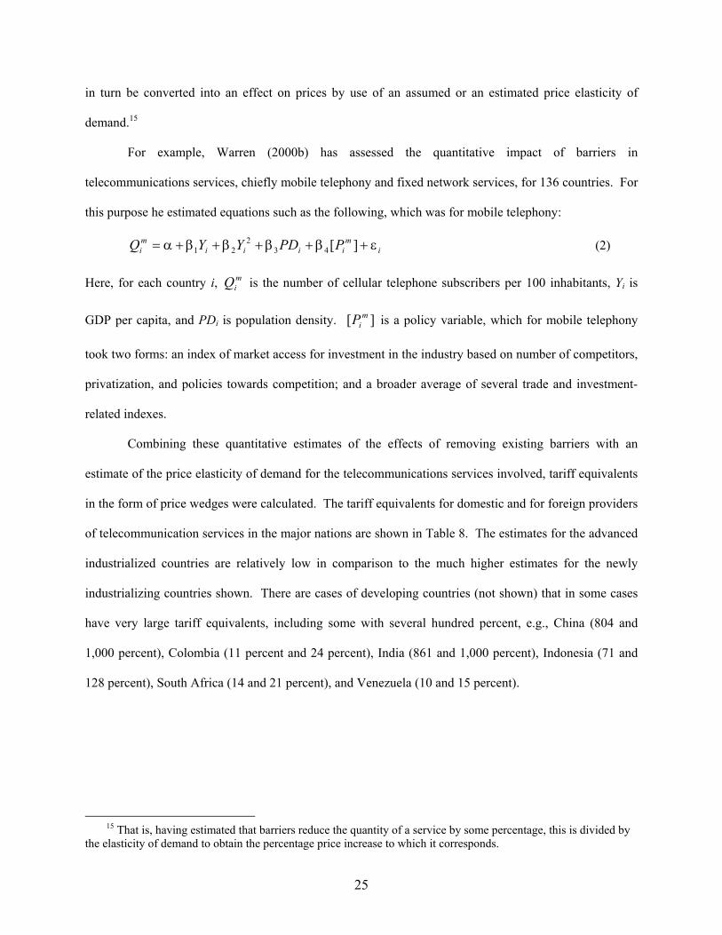
For example, Warren (2000b) has assessed the quantitative impact of barriers in

telecommunications services, chiefly mobile telephony and fixed network services, for 136 countries. For

this purpose he estimated equations such as the following, which was for mobile telephony:

im

iiiimi PPDYYQ ε+β+β+β+β+α= ][43

221 (2)

Here, for each country i, miQ is the number of cellular telephone subscribers per 100 inhabitants, Yi is

GDP per capita, and PDi is population density. ][ miP is a policy variable, which for mobile telephony

took two forms: an index of market access for investment in the industry based on number of competitors,

privatization, and policies towards competition; and a broader average of several trade and investment-

related indexes.

Combining these quantitative estimates of the effects of removing existing barriers with an

estimate of the price elasticity of demand for the telecommunications services involved, tariff equivalents

in the form of price wedges were calculated. The tariff equivalents for domestic and for foreign providers

of telecommunication services in the major nations are shown in Table 8. The estimates for the advanced

industrialized countries are relatively low in comparison to the much higher estimates for the newly

industrializing countries shown. There are cases of developing countries (not shown) that in some cases

have very large tariff equivalents, including some with several hundred percent, e.g., China (804 and

1,000 percent), Colombia (11 percent and 24 percent), India (861 and 1,000 percent), Indonesia (71 and

128 percent), South Africa (14 and 21 percent), and Venezuela (10 and 15 percent).

15 That is, having estimated that barriers reduce the quantity of a service by some percentage, this is divided by

the elasticity of demand to obtain the percentage price increase to which it corresponds.

26

Gravity-Model Estimates

Because the modeling of prices that is needed to estimate a price effect above is necessarily very

sector specific, the techniques described so far have limited use for quantifying barriers across sectors.

Likewise, they are not useful for comparing the overall levels of service trade barriers across countries.

For that, one needs a more general model of trade to use as a benchmark, and the natural choice is the so-

called gravity model. This model relates bilateral trade volumes positively to the incomes of both trading

partners, and also negatively to the distance between them.16 It has become a very popular tool in recent

years for eliciting the effects of a wide variety of policy and structural influences on trade in a manner

that controls for the obvious importance of income and distance.

Francois (1999) has fit a gravity model to bilateral services trade for the United States and its

major trading partners, taking Hong Kong and Singapore to be free trade benchmarks. The independent

variables, in addition to distance between trading partners, included per capita income, gross domestic

product (GDP), and a Western Hemisphere dummy variable. The differences between actual and

predicted imports were taken to be indicative of trade barriers and were then normalized relative to the

free trade benchmarks for Hong Kong and Singapore. Combining this with an assumed demand elasticity

of 4, tariff equivalents can be estimated. The results for business/financial services and for construction

are indicated in Table 9. Brazil has the highest estimated tariff equivalent for business/financial services

(35.7 percent), followed by Japan, China, Other South Asia, and Turkey at about 20 percent. The

estimated tariff equivalents are considerably higher for construction services, in the 40-60 percent range

for China, South Asia, Brazil, Turkey, Central Europe, Russia, and South Africa, and in the 10-30 percent

range for the industrialized countries. Further details are given in Appendix A on the limitations of the

use and interpretation of gravity models.

16 Typically, the log of the volume of total bilateral trade between two countries is regressed on the logs of their

national incomes, the log of distance between them, and other variables such as per capita income and dummy variables to reflect a common border, common language, etc.

27

Financial-Based Measurements

Hoekman (2000) has suggested that financial data on gross operating margins calculated by

sector and country may provide information about the effects of government policies on firm entry and

conditions of competition.17 As he notes (p. 36):

“In general, a large number of factors will determine the ability of firms to generate high margins, including market size (number of firms), the business cycle, the state of competition, policy enforcement, the substitutability of products, fixed costs, etc. Notwithstanding the impossibility of inferring that high margins are due to high barriers, there should be a correlation between the two across countries for any given sector. Data on operating margins provide some sense of the relative profitability of activities, and therefore, the relative magnitude (restrictiveness) of barriers to entry/exit that may exist.”

The country-region results of Hoekman’s analysis, averaged over firms and sectors for 1994-96,

are indicated for agriculture, manufacturing, and services in Table 10. Sectoral results for services only

are given in Table 11. Services margins are generally higher than manufacturing margins by 10-15

percentage points, and the services margins vary considerably across countries. Australia, Hong Kong,

and Singapore have the lowest services margins – in the neighborhood of 20 percent – while Chile, China,

Indonesia, Philippines, Taiwan, Thailand, and the United States have services margins in excess of 40

percent. The sectoral results indicate that the margins for hotels and financial services are relatively high,

and the margins for wholesale and retail trade are lower. The margins for several developing countries

appear to be relatively high in a number of sectors. Overall, as Hoekman suggests (p. 39):

“…business services, consultancy, and distribution do not appear to be among the most protected sectors. …barriers to competition are higher in transportation, finance, and telecommunications. These are also basic ‘backbone’ imports that are crucial for the ability of enterprises to compete internationally.”

Diversity of Methods

As should be clear from the foregoing, studies of services barriers have used a wide variety of

approaches. This is not surprising given the wide variety of the service industries themselves and the

variation across them in the data that may be available. In our concluding section, below, we will outline

17Gross operating margins are defined as total sales revenue minus total average costs divided by total average

costs.

28

the steps that seem to have been most commonly used and/or successful in the largest number of studies,

as a guide to those who intend to replicate their work in other industries and countries. However, it will

often be the case that one or more of these steps cannot be followed in particular cases. Research on

services barriers must therefore often make do with whatever information may be available. As

illustrated by the studies discussed here, this may require creative exploitation of seemingly heroic

assumptions in order to extract any information at all.

V. Measuring the Economic Consequences of Liberalizing Services Barriers

Issues to be Addressed: • Sectoral modeling • CGE modeling

While the various measurements of services barriers that we have reviewed are of interest in

themselves, they need to be incorporated into an explicit economic modeling framework in order to

determine how the existence or removal of the barriers will affect conditions of competition, productivity,

the allocation of resources, and economic welfare within or between sectors and countries. In this regard,

a modeling framework can be devised for individual sectors or on an economy-wide basis using

computable general equilibrium (CGE) modeling.

Sectoral Modeling

An example of sectoral modeling is provided by Fink, Mattoo, and Rathindram (2003), who

analyze the impact of policy reform on sectoral performance in basic telecommunications. Their data

cover 86 developing countries globally for the period, 1985-1999. They address three questions, covering

the impact of: (1) policy changes relating to ownership, competition, and regulation; (2) any one policy

reform coupled with the implementation of complementary reforms; and (3) the sequencing of reforms.

Their findings are: (1) privatization and the introduction of competition significantly increase

labor productivity and the density of telecommunication mainlines; (2) privatization and competition

work best through their interactions; and (3) there are more favorable effects from introducing

29

competition before privatization. They further conclude that autonomous technological progress

outweighs the effects of policy reforms in increasing the growth of teledensity.

What is especially noteworthy about this type of study is its focus on both the policy and market

structure of the sector and the econometric framework that is designed to measure the determinants of

teledensity and telecommunications productivity. The assessment of particular services barriers may

therefore be most effectively addressed when incorporated into a sectoral modeling framework.18

CGE Modeling

In contrast to sectoral modeling, CGE modeling provides a framework for multi-sectoral and

multi-country analysis of the economic effects of services barriers and related policies. Most CGE

modeling research to date has been focused on barriers to international trade in goods rather than trade in

services and FDI. The reasons for this stem in large part from the lack of comprehensive data on cross-

border services trade and FDI and the associated barriers, together with the difficult conceptual problems

of modeling that are encountered. Some indication of pertinent CGE modeling work relating to services

is provided in Hardin and Holmes (1996, p. 85), Brown and Stern (2001, pp. 272-74), and Stern (2002,

pp. 254-56). The approaches to modeling can be divided as follows: (1) analysis of cross-border services

trade liberalization in response to reductions in services barriers; (2) modeling in which FDI is assumed to

result from trade liberalization or other exogenous changes that generate international capital flows in the

form of FDI in response to changes in rates of return; and (3) modeling of links between multinational

corporations’ (MNCs) parents and affiliates and distinctions between foreign and domestic firms in a

given country/region.

The third type of CGE modeling study just noted comes closest to capturing the important role

played especially by MNCs and their foreign affiliates in providing Mode 3-type services. This, for

example, is the focus of the study by Brown and Stern (2001), some details of which are presented in

Appendix A below. Brown and Stern analyze the effects of removal of services barriers under alternative

18 See also Fink, Mattoo, and Neagu (2002) and Appendix A below for a summary of their study of the importance of restrictive trade policies and private anti-competitive practices relating to international maritime services.

30

conditions of international capital mobility and changes in the world capital stock due to increased

investment. Their results, presented in Table A-7, suggest that the welfare effects of removing services

barriers are sizable and vary across countries depending on how international capital movements and

changes in domestic investment respond to changes in rates of return. The largest potential benefits are

realized for all of the major developed and developing countries when allowance is made for changes in

investment that augment the stock of capital

.

VI. Guideline Principles and Recommended Procedures for Measuring Services Barriers and for Assessing the Consequences of Their Liberalization

As a summary of what we have reported in detail here about the methodologies for measuring

services barriers and using these measurements to assess the consequences of liberalization in services,

we conclude first with several principles to be kept in mind during this process and then with more

detailed procedural steps that we recommend should be followed:

Principles:

1. Most barriers to trade and investment in services take the form of domestic regulations, rather

than measures at the border.

2. No single methodology is sufficient for documenting and measuring barriers to trade in

services. Instead, investigators need to draw upon all available information, including both

direct observation of particular barriers and indirect inference of barriers using data on prices

and quantities.

3. Because of the special role of incumbent firms in many service industries, regulations do not

need to be explicitly discriminatory against foreign firms in order to have discriminatory

effects.

Procedures:

1. Collect the details of domestic regulations and related policies affecting services firms in the

countries and/or sectors being examined, including the manner in which they apply to foreign

31

versus domestic firms, plus quantitative details of their application, such as any percentage or

dollar limits that they impose.

2. Ideally, this information should be collected by systematic surveys of governments and/or

firms. However, it may also be possible to infer it less directly from documents prepared for

other purposes, such as the commitments that governments made to the GATS in the Uruguay

Round and subsequent negotiations.

3. For each type of regulation or policy, define degrees of restrictiveness and assign scores to

each, ranging from zero for least restrictive to one for most restrictive.

4. Construct a measure of restrictiveness by: weighting the scores from step 3 based on

judgments of the relative importance of each policy; using a statistical methodology such as

factor analysis that will serve to identify the weights; or designing proxy measures, such as

dummy variables, to represent particular restrictions. The resulting measures can then be

used directly for reporting the presence and importance of barriers across industries and

countries, as well as for providing an input to subsequent analysis.

5. Convert the measures of restrictiveness from step 4 into a set of tariff equivalents by one or

more of the following methods. Depending on the quality of information that goes into their

construction, these tariff equivalents may be superior to the measures themselves for

reporting about barriers and analyzing their effects.

a. Assign judgmental tariff-equivalent values to each of the component measures,

representing the percentage taxes on foreign suppliers to which each component is

thought to correspond at their most restrictive levels (index = 1).

b. Use data on prices and their determinants as the basis for a regression model that includes

an index or other measures of restrictiveness and that estimates the effect on prices.

c. Use data on quantities produced or traded as the basis for a regression model that

includes an index or other measures of restrictiveness and that estimates the effect on

32

quantities. This estimate can then be converted to tariff equivalents using an assumed or

estimated price elasticity of demand.

6. Use an index or other measures of restrictiveness or the tariff equivalents constructed above

as inputs into a model of production and trade in order to ascertain the effects of changes in

the barriers to which they correspond. The appropriate model for this purpose depends on

whether sectoral or economy-wide policy changes are to be analyzed. For economy-wide

policy changes, the model should be a general equilibrium one, incorporating the full effects

of barriers across sectors and countries. Ideally, too, the model should be designed to capture

the effects of service regulations in the form that they have been observed and quantified as

above.

33

Appendix A

Literature Summaries of Methods of Measurement

In this appendix, we provide a somewhat more technical discussion of the various methods of

measurement of services barriers, focusing especially on available studies that have been completed and

that can be consulted for more information on methodology and data and possible adaptation in further

research.

A-1: Frequency Studies and Indexes of Restrictiveness

In what follows, we summarize several studies that complement our discussion in the main text:

• Mattoo (1998) analyzed market access commitments in financial services, covering direct insurance and banking. His results indicated that Latin America was the most restricted in direct insurance and Asia the most restricted in banking services.

• Marko (1998) constructed frequency measures for the basic telecommunications markets, using Hoekman’s (1995) methodology. Marko found that 58% of the basic telecommunications services market for the 69 signatories of the February 1997 Agreement on Basic Telecommunications was covered by partial or full GATS commitments.

• McGuire (1998) showed that Australia’s impediments in financial services, including banking, securities, and insurance, were much lower as compared to other economies in Asia.

• Colecchia (2000) provided a methodological, pilot study of the barriers on accountancy services for Australia, France, the United Kingdom, and the United States, using OECD information on regulatory regimes for 1997. The United Kingdom was found to be the most liberal, the United States the least liberal.

• Kalirajan (2000) constructed restrictiveness indexes for 38 economies, using GATS schedules and a variety of other information on barriers to distribution services as of June 1999. The indexes covered the services of commission agents, wholesalers, retailers, and franchisers. The findings were that: (1) Belgium, India, Indonesia, France, Korea, Malaysia, the Philippines, Switzerland, and Thailand were the most restrictive economies and Singapore and Hong Kong the most open; and (2) the countries that were the most discriminatory against foreign firms included Malaysia, the Philippines, Venezuela, Brazil, the United States, and Greece. The detailed domestic and foreign restrictiveness indexes were broken down by country and are available on the Productivity Commission website.

• Kemp (2000) constructed restrictiveness indexes for the four modes of providing educational services, using GATS data on commitments for market access and national treatment for the five sub-sectors of educational services and covering 29 countries. While only a quarter of GATS member countries scheduled commitments, the evidence suggested that consumption abroad, which is the major mode of educational trade in terms of foreign-student tuition, fees, and expenditures, was comparatively the least restricted mode.

34

• McGuire, Schuele, and Smith (2000) developed indexes for restrictions on foreign maritime service suppliers and all maritime service suppliers covering 35 economies during the period 1994-98, using a variety of GATS and other data sources. They found that: (1) Brazil, Chile, India, Indonesia, Korea, Malaysia, the Philippines, and the United States had the most restricted markets against foreign maritime suppliers; and (2) Chile, the Philippines, Thailand, Turkey, and the United States were the most discriminatory in favoring domestic suppliers. The detailed domestic and foreign indexes of restrictiveness were broken down by country and are available on the Productivity Commission website.

• Nguyen-Hong (2000) constructed restrictiveness indexes for accountancy, architectural, and engineering services for 34 economies and legal services for 29 economies. The indexes were compiled from WTO, OECD, APEC, and a variety of other sources. The findings were that: (1) legal and accounting were the most highly restricted services; (2) Indonesia, Malaysia, Austria, Mexico, and Turkey were the most restrictive for the four professions, and Finland and the Netherlands the most open; (3) nationality requirements were the most extensive in legal and accountancy services; (4) residency requirements were common in accountancy services; (5) partnerships and practices between accountants and lawyers were commonly restricted; and (6) recognition of foreign qualifications and licenses was subject to a variety of restrictions among countries. The detailed domestic and foreign restrictiveness indexes were broken down and are available on the Productivity Commission website.

• Warren (2000a) used data for 136 countries from the International Telecommunications Union (ITU) to construct five indexes for the regulation of telecommunications policies that discriminate against: (1) all potential providers of cross-border telecommunications services; (2) foreign providers of cross-border services; (3) all potential providers of fixed network services; (4) all potential providers of cellular services via FDI; and (5) foreign providers of mobile services via FDI. He found: (1) significant variation across countries in all five indexes; (2) most countries relied only on foreign carriers to provide competition in mobile markets; (3) countries were less prepared to use majority-owned foreign carriers in their fixed network markets; (4) countries that liberalized their mobile networks were more likely to liberalize their fixed networks; (5) countries that limited commercial presence via FDI were more liberal in permitting cross-border entry; and (6) GATS-based indexes that tended to reflect legal conditions, as calculated by Marko (1998), were not altogether well correlated with ITU-based indexes that were designed to reflect economic conditions. The detailed domestic and foreign indexes by country are available on the Productivity Commission website.

• Doove, Gabbitas, Nguyen-Hong, and Owen (2001) constructed restrictiveness indexes for international air passenger transport, telecommunications, and electricity supply. The index for air transport was an average of the bilateral restrictiveness indexes applicable to pairs of countries. The data covered 875 airline routes for 35 economies and refered to the late 1990s. The bilateral restrictions included designation, capacity, fares, and charter services, with weights derived using factor analysis in an OECD study by Gonenc and Nicoletti (2001). The bilateral restrictions were generally not covered under the GATS, so that discriminatory restrictions on third countries may have been applied. The results are shown in column (2) of Table 7 and indicate substantial variation across countries as a consequence of the agreement-specific bilateral restrictions.

35

The restrictiveness index for telecommunications covered 24 OECD member countries and 23 non-OECD countries, using data for 1997. The telecommunications industry has been undergoing rapid technological change in recent decades, and there has been widespread regulatory reform and structural reform undertaken in many countries. Doove et al. built upon the OECD study by Boylaud and Nicoletti (2000), who focused on the four major telecommunications sectors: trunk (domestic long distance); international (international long distance); mobile (cellular); and leased-line services. The regulatory measures covered include: market share of new entrants; index of governmental control of the public telecommunications operators (PTOs); degree of internationalization of domestic markets; time to liberalization; and time to privatization. These measurements were incorporated into an econometric framework for the individual sectors in order to estimate the price impacts involved that are noted in Table A-1.

Electricity supply has also been undergoing significant deregulation and structural reform. Building upon OECD work by Steiner (2000), Doove et al. assembled data for 50 economies for 1996. The regulatory measures covered were: unbundling of electricity generation from transmission; third party access; presence of a wholesale electricity market; degree of private/public ownership; time to liberalization; and time to privatization. The price impacts of regulation were estimated and are indicated in Table A-2.

A-2: Price-Impact Studies We summarize below a number of other pertinent studies of price-impacts that may be consulted

for further technical details and results:

• Johnson, Gregan, Gentle, and Belin (2000) noted that international air services are regulated by means of bilateral agreements and are largely excluded from the GATS. They developed a partial-equilibrium, spatial econometric model that was used to analyze the effects on prices, quantities, and economic welfare, in Australia and foreign countries, of the entry of a new airline (Ansett) into the Australian market, as well as plurilateral reform for an “open club” for airlines among Australia, China, Hong Kong, and Japan. They showed that there were significant benefits realized from the entry of new competitors into the airline markets. Also, members of an open club gained, but at the expense of non-members.

• Kalirajan (2000) used firm-level accounting data for wholesale and retail food

distributors in 18 economies to indicate the relationship between trade restrictiveness and distributors’ price-cost margins. The results suggested that the restrictions were primarily cost creating rather than rent creating and were accounted for mainly by restrictions on establishment. Using the restrictiveness indexes, coefficient estimates, and sample means, the estimated cost impacts noted in Table A-3 range between 0 and 8 percent.

• Kalirajan, McGuire, Nguyen-Hong, and Schuele (2000) developed and estimated a

model applied to 694 banks in 27 economies for 1996-97 to assess the impact of non-prudential restrictions on the interest margins of banks. The net interest margin is the difference between a bank’s lending and deposit rates. A two-stage procedure

36

was used for estimation purposes. In the first stage, bank-specific variables were used to explain the interest margins in all the economies, and, in a second stage, cross-country estimation was used to take economy-wide variables into account. The foreign and domestic restrictiveness indexes calculated in McGuire and Schuele (2000) entered into the second-stage estimation. The foreign restrictiveness index was found to be a significant determinant of interest rate spreads, while the domestic restrictiveness index was not significant. The price impacts of the restrictions were calculated from the second-stage results and are presented in Table A-4. Chile, Indonesia, Malaysia, the Philippines, Singapore, South Korea, and Thailand have the highest price impacts due to the restrictions on foreign banks.

• Kang (2000) investigated the impact of restrictions on maritime services, using a

partial-equilibrium econometric model that incorporated cross-country and bilateral trade data as determinants of demand for these services. Shipping margins for manufactured goods were derived from FOB/CIF value differentials and were used as a proxy for price. The shipping margins were to be explained by bilateral restrictions, distance, and the scale of bilateral trade. Indexes for 23 countries were adapted from McGuire, Schuele, and Smith (2000), and the remaining data were from the 1995 database of the Global Trade Analysis Project (GTAP). The foreign index of restrictiveness was decomposed into measures affecting commercial presence and into other restrictions such as on cabotage and port services. Allowance was also made for different bilateral relationships as between industrialized and developing economies. The most important conclusion reached was that a low degree of restrictions in any trading partner was necessary in order to have low shipping charges. Further, low-income countries stood to gain the most from eliminating restrictions on shipping services.

• Nguyen-Hong (2000) estimated the influences of restrictions on the price-cost

margins of 84 engineering service firms in 20 economies, using 1996 company accounting data compiled from a variety of private and official sources. A model of firm behavior was developed to include the determinants of the observed price-cost margins, and a linear version using ordinary least squares was implemented with cross-section data. The index of foreign barriers to establishment was highly significant and had a positive and statistically significant impact on price-cost margins. The index of domestic barriers to establishment had a negative and significant impact. The price and cost impacts of the restrictions were calculated, using the actual indexes of restrictiveness, estimated coefficients, and the sample means of the independent variables. The price impacts, which are summarized by country in Table A-5, exceed 10 percent for Austria, Mexico, Malaysia, Indonesia, and Germany. The cost impacts are relatively small, ranging between 0.7 and 6.8 percent. The price and cost impacts were also calculated by types of barriers.

• Trewin (2000) used time-series data on the total costs of providing

telecommunications services for 37 countries obtained from the International Telecommunications Union (ITU) for the period 1982-92. He used a frontier cost method as a means of estimating the minimum possible costs that are expended from a given combination of inputs. The distance of an observation above the cost frontier is a measurement of the degree of technical inefficiency. The measurements of restrictiveness calculated by Marko (1998) and Warren (2000a) were used in the estimation process. The results suggested that countries that provide higher levels of FDI face lower costs. Making allowance for the quality-cost aspects of

37

telecommunication services reinforced the importance of the cost impacts of restrictions. When the sample was divided between low and high income countries, the average efficiency of the high income set was more than three times better than the low income set. The results are listed in Table A-6. It can be seen, in the high income set, that Luxembourg is close to the efficiency frontier whereas Portugal and Korea are relatively high cost countries.

• Doove, Gabbitas, Nguyen-Hong, and Owen (2001) constructed restrictiveness

indexes and estimates of price impacts for international air passenger transport, telecommunications, and electricity supply. Their indexes of bilateral restrictions on international air passenger transport referred to 35 economies in the Asia-Pacific, Americas, and European regions. Focusing on the discount segment of the air passenger market, they implement a procedure for estimating the price effects of the applicable restrictions, using fare data primarily for the end years of the 1990s. The results, which are shown above in Table 7, indicated that the higher price effects range from 12 to 22 percent in the Asia-Pacific economies, 9 to 18 percent in the Americas, and generally below 10 percent in the European economies. The price impacts for business and economy airfares were considerably higher but should be interpreted tentatively due to data constraints.

Measurements of the impact of telecommunications regulations were derived for 24 OECD and 23 other countries, using data for 1997. Price-impact measurements of regulation were calculated for four major sectors of telecommunications, including trunk, international, mobile, and leasing services and are listed by country and type of service in Table A-1. While the results suggested that countries with more stringent regulatory regimes tended to have higher telecommunications prices, the authors noted that there were several cases in which the results appeared to be counter intuitive and sensitive to small changes in the data. The reported results should therefore be treated with caution, pending further clarification and improvement of the model and data that were used. Measurements of regulation and impacts on industrial electricity prices for 50 economies, using 1996 data, were developed. The estimated price impacts are listed by country in Table A-2. The impacts ranged from 0 to 35 percent, with a mean of 13 percent and a standard deviation of 13 percent. The authors noted, however, that the estimated price impacts were quite sensitive to the methodology and data used and therefore should be treated as ordinal rankings rather than absolute values.

• Fink, Mattoo, and Neagu (2002) analyzed the importance of restrictive trade policies

and private anti-competitive practices for international maritime services. For this purpose, they used data on U.S. imports carried by liners from 59 countries that accounted for about 65 percent of the total value of U.S. maritime imports in 1998. While restrictions on the provision of port services were found to be significant, private anti-competitive practices involving collusion among international maritime cartels were shown to have a considerably greater influence on maritime transport prices.

38

A-3: Gravity-Model Estimates

Deardorff and Stern (1998, p. 24) have noted that measurements based on the gravity model are

useful mainly in identifying relative levels of protection across sectors and countries. But gravity models

have some important drawbacks. That is, by attributing to trade barriers all departures of trade from what

the included variables can explain, there is a great burden on the model being used. Thus, the worse the

model, the more likely it is that trade barrier estimates will have an upward bias.

An additional problem exists when this technique is used to infer barriers for separate industries.

The theoretical basis for the gravity equation, as in Anderson (1979) and Deardorff (1998), applies to total

trade, not to trade in individual sectors. The gravity equation makes sense at the sectoral level only if all

countries are equal in their capacity to produce in a sector, which of course would be a denial of the role

of comparative advantage. Thus, if a country were in fact to have a comparative advantage in a particular

service sector, so that its output would be high and its cost of serving its domestic market itself would be

low, then it will import less from abroad than would be expected based on income and distance alone.

Thus comparative advantage may show up as an implicit barrier to trade, when in fact none exists.

A-4: Computable General Equilibrium (CGE) Modeling

In the study by Brown and Stern (2001), each MNC is assumed to produce a differentiated

product and to allocate production to its various host-country locations. The monopolistically

competitive firms employ capital, labor, and intermediate inputs in their production, and they set prices as

an optimal mark-up of price over marginal cost. The number of firms is permitted to vary to hold MNC

profits at zero. Consumers are assumed to allocate their expenditure between goods and services that are

produced by firms domestically and varieties that are imported from each national source. Labor is taken

to be freely mobile among domestic sectors but not across borders. Capital, however, is mobile

internationally, although not perfectly so, because there is a risk premium that will vary depending on the

size of a country’s capital stock.

39

Barriers to FDI are assumed to take the form of an increased cost of locating investment in a host

country. For this purpose, Brown and Stern use the cost-price margins estimated by Hoekman (2000),

which have been discussed above and are listed in Tables 10 and 11, as indicative of barriers to FDI.

Since the cost-price gap is smallest in most sectors in Hong Kong, a country thought to be freely open to

foreign firms, the excess in any other country above the Hong Kong figure is taken to be due to barriers to

the establishment of foreign firms.

Using the aforementioned modeling structure with three sectors (agriculture, manufactures, and

services) and 18 countries/regions, Brown and Stern calculate the economic effects of removal of services

barriers according to the following three scenarios:19

Scenario A: Removal of services barriers, with perfect international capital mobility and fixed world capital stock.

Scenario B: Removal of services barriers, with risk-premium elasticity = 0.1 to allow for imperfect capital mobility, and fixed world capital stock.

Scenario C: Removal of services barriers, with risk-premium elasticity = 0.1 to allow for imperfect capital mobility, and world capital stock increased by 3%.

When barriers are lowered, international capital in the form of FDI will then be attracted to countries with

the relatively highest rates of return and away from other countries.

The welfare effects, as a percentage of GNP and in billions of dollars, resulting from the assumed

removal of the services barriers for each of the three scenarios are listed in Table A-7 for the

countries/regions covered by the model.20 When services barriers are lowered, international capital in the

form of FDI will then be attracted to countries with the highest rates of return and away from other

countries.

19 See also studies undertaken at the Australian Productivity Commission by Dee and Hanslow (2001) and

Verikios and Zhang (2001) for computational results based on a related modeling framework and with estimates of services barriers taken from Kalirajan et al. (2000) and Warren (2000 a,b).

20 See Brown and Stern (2001, pp. 277-78) for the results for the absolute changes in imports and exports, the percentage change in the terms of trade, and the percentage change in the real wage. The sectoral results for the three aggregated sectors for Scenario C are reported in Brown and Stern (pp. 281-82). They show that output increases economy-wide in just about every sector in all countries/regions, and there is a wide prevalence of the realization of economies of scale. There are also generally significant increases in activity by foreign-owned affiliates, especially in the countries that record large increases in output.

40

It is evident in Table A-7 that the welfare effects of removing the services barriers are sizable and

that they vary markedly across countries. For the industrialized countries in Scenario A with perfect

international capital mobility, the largest increases are for Canada, $84.0 billion (14.8% of GNP), the

European Union (EU), $42.4 billion (0.5% of GNP), and the United States, $35.0 billion (0.5% of GNP).

Because it loses capital, Japan has a decline of $103.7 billion (2.0% of GNP). Among the developing

countries, the largest increases are for Indonesia, $30.8 billion (15.6% of GNP), China, $26.9 billion

(3.8% of GNP), and Taiwan, $20.7 billion, $7.6% of GNP). It is also evident that there are declines in

welfare for a number of developing countries, in particular, Korea, Thailand, Chile, Mexico, and the Rest

of Cairns Group. What is reflected in the results is that welfare is affected by whether or not a country

attracts or loses capital as a result of services liberalization. Countries that lose capital become “smaller”

in the economic sense of the word. As the economy contracts, surviving firms produce less than before.

The fall in firm output generally occurs in order to avoid a large loss in variety of domestically produced

goods. The subsequent economy-wide reduction in scale economies is usually the source of the welfare

loss.

The results in Scenario A are sensitive to the assumption of perfect capital mobility. As noted

above, countries that import capital are assumed to pay a risk premium that is a function of capital

imports. The elasticity of the risk premium with respect to the volume of capital imports can be set

exogenously in the model. Thus, in Scenario B, Brown and Stern assume that capital imports that result

in a 1% increase in the capital stock generate an interest-rate risk premium of 0.1%. That is, the risk-

premium elasticity is 0.1%. It is apparent from the results for Scenario B in Table A-7 that the

introduction of a risk premium that reflects a decrease in international capital mobility has the effect of

reducing the welfare effects of services liberalization as compared to Scenario A, in which there was

perfect capital mobility.

In both Scenarios A and B, there is a rise in the real return to capital. Therefore, it is likely that,

over time, there will be an increase in the world’s capital stock as savers and investors respond to the

increased incentive to accumulate capital. To take this into account, in Scenario C, with the risk premium

41

elasticity remaining at 0.1%, Brown and Stern allow for an increase in the world’s capital stock by 3%.

This is the amount necessary to hold the real return to capital equal to the level in the base period. As can

be seen in Table A-7, the welfare effects of services liberalization are now positive for all of the countries

shown. For the world as a whole, welfare rises by $703.7 billion. Canada’s welfare increases by $85.0

billion (14.9% of GNP), the EU by $202.4 billion (2.5% of GNP), and the United States, $222.5 billion

(3.1% of GNP). There are also sizable absolute and percentage increases for the developing countries, in

particular China, Indonesia, Taiwan, and Hong Kong. It is further noteworthy that welfare increases for

all of the countries/regions shown.

It is evident accordingly that these welfare effects associated with an increase in the world’s

capital stock in response to an increase in the rate of return to capital are considerably larger than what is

commonly seen in CGE models in which capital is assumed to be internationally immobile.21 This may

not be surprising because it has been apparent from previous CGE analyses of trade liberalization that

have made allowance for international capital flows that the largest welfare gains stem from these flows

rather than from the removal of tariffs and other trade barriers that distort consumer choice in goods

trade.22

The understanding of the consequences of liberalizing services barriers thus is enhanced when

allowance is made for the behavior of multinational firms whose foreign affiliates are already located in

or attracted to host countries. When services liberalization occurs and the real return to capital is

increased, so that there are FDI (Mode 3) international capital flows and the world capital stock expands,

most countries stand to gain significantly in terms of economic welfare.

21 Compare, for example, the results of the Michigan Model reported in Brown, Deardorff, and Stern (2003). 22 See Brown, Deardorff, and Stern (1992).

42

References

Anderson, James E. 1979 "A Theoretical Foundation for the Gravity Equation," American Economic

Review 69, (March), pp. 106-116.

Bosworth, Malcolm, Christopher Findlay, Ray Trewin, and Tony Warren. 2000. “Price-impact Measures of Impediments to Services Trade,” in Christopher Findlay and Tony Warren (eds.), Impediments to Trade in Services: Measurement and Policy Implications. London and New York: Routledge.

Boylaud, O. and G. Nicoletti. 2000. “Regulation, Market Structure and Performance in Telecommunications,” Working Paper No. 237ECO/WKP (2000), 10, Economics Department, OECD, Paris, 12 April.

Brown, Drusilla and Robert M. Stern. 2001. “Measurement and Modeling of the Economic Effects of Trade and Investment Barriers in Services,” Review of International Economics 9:262-86

Colecchia, Alessandra. 2000. “Measuring Barriers to Market Access for Services: A Pilot Study on Accountancy Services,” in Christopher Findlay and Tony Warren (eds.), Impediments to Trade in Services: Measurement and Policy Implications. London and New York: Routledge.

Deardorff, Alan V. “Determinants of Bilateral Trade: Does Gravity Work in a Neoclassical World?” in Jeffrey A. Frankel, ed., The Regionalization of the World Economy, Chicago: University of Chicago Press, 1998.

Deardorff, Alan V. and Robert M. Stern. 1998. Measurement of Nontariff Barriers. Ann Arbor: University of Michigan Press.

Dee, Philippa and Kevin Hanslow. 2001. “Multilateral Liberalization of Services Trade,” in Robert M. Stern (ed.), Services in the International Economy. Ann Arbor: University of Michigan Press.

Dee, Philippa, Alexis Hardin, and Leanne Holmes. 2000. “Issues in the Application of CGE Models to Services Trade Liberalization,” in Christopher Findlay and Tony Warren (eds.), Impediments to Trade in Services: Measurement and Policy Implications. London and New York: Routledge.

Disclosure. 1998. Global Researcher – Worldschope Database. Bethesda, Maryland: Disclosure.

Doove, Samantha, Owen Gaabbitas, Duc Nguyen-Hong, and Joe Owen. 2001. “Price Effects of Regulation: Telecommunications, Air Passenger Transport and Electricity Supply,” Productivity Commission Staff Research Paper, AusInfo, Canberra (October).

Findlay, Christopher and Tony Warren (eds.). 2000. Impediments to Trade in Services: Measurement and Policy Implications. London and New York: Routledge.

Fink, Carsten, Aaditya Mattoo, and Ileana Cristina Neagu. 2002. “Trade in International Maritime Services: How Much Does Policy Matter?” World Bank Economic Review 16:81-108.

Fink, Carsten, Aaditya Mattoo, and Randeep Rathindran. 2003. “An Assessment of Telecommunications Reform in Developing Countries,” Information Economics and Policy 15:443-66.

43

Francois, Joseph. 1999. “Estimates of Barriers to Trade in Services,” Erasmus University, unpublished manuscript.

Gonenc, R. and G. Nicoletti. 2001. “Regulation, Market Structure and Performance in Air Passenger Transportation,” OECD Economic Studies, No. 32, OECD, Paris.

Hardin, Alexis and Leanne Holmes. 1997. Services Trade and Foreign Direct Investment. Staff Research Paper, Industry Commission. Canberra: Australian Government Publishing Services.

Hoekman, Bernard. 1995. “Assessing the General Agreement on Trade in Services,” in Will Martin and L. Alan Winters (eds.), The Uruguay Round and the Developing Countries, World Bank Discussion Paper No. 307. Washington, D.C.: The World Bank. Revised version published in Will Martin and L. Alan Winters (eds.), Cambridge University Press, 1996.

Hoekman, Bernard. 2000. “The Next Round of Services Negotiations: Identifying Priorities and Options,” Federal Reserve Bank of St. Louis Review 82:31-47.

Hoekman, Bernard and Carlos A. Primo Braga. 1997. “Protection and Trade in Services: A Survey,” Open Economies Review 8:285-308.

Holmes, Leanne and Alexis Hardin. 2000. “Assessing Barriers to Services Sector Investment,” in Christopher Findlay and Tony Warren (eds.), Impediments to Trade in Services: Measurement and Policy Implications. London and New York: Routledge.

Johnson, Martin, Tendar Gregan, Geraldine Gentle, and Paul Belin. 2000. “Modeling the Benefits of Increasing Competition in International Air Services,” in Christopher Findlay and Tony Warren (eds.), Impediments to Trade in Services: Measurement and Policy Implications. London and New York: Routledge

Kalirajan, Kaleeswaran. 2000. “Restrictions on Trade in Distribution Services,” Productivity Commission Staff Research Paper, AusInfo, Canberra (August).

Kalirajan, Kaleeswaran, Greg McGuire, Duc Nguyen-Hong, and Michael Schuele. 2000. “The Price Impact of Restrictions on Banking Services,” in Christopher Findlay and Tony Warren (eds.), Impediments to Trade in Services: Measurement and Policy Implications. London and New York: Routledge.

Kang, Jong-Soon. 2000. “Price Impact of Restrictions on Maritime Transport Services,” in Christopher Findlay and Tony Warren (eds.), Impediments to Trade in Services: Measurement and Policy Implications. London and New York: Routledge.

Karsenty, Guy. 2000. “Just How Big Are the Stakes? An Assessment of Trade in Services by Mode of Supply,” in Pierre Sauvé and Robert M. Stern (eds.), Services 2000: New Directions in Services Trade Liberalization. Washington, D.C.: Brookings Institution.

Kemp, Steven. 2000. “Trade in Education Services and the Impacts of Barriers on Trade,” in Christopher Findlay and Tony Warren (eds.), Impediments to Trade in Services: Measurement and Policy Implications. London and New York: Routledge.

Marko, M. 1998. “An Evaluation of the Basic Telecommunications Services Agreement, CIES Policy Discussion Paper 98/09, Centre for International Economic Studies, University of Adelaide.

44

Mattoo, Aaditya. 1998. “Financial Services and the WTO: Liberalization in the Developing and Transition Economies,” for presentation at the Workshop, “Measuring Impediments to Trade in Services,” Productivity Commission, Canberra, April 30 – May 1, 1998.

McGuire, Greg. 1998. Australia’s Restrictions on Trade in Financial Services. Staff Research Paper, Productivity Commission, Canberra.

McGuire, Greg and Michael Schuele. 2000. “Restrictiveness of International Trade in Banking Services,” in Christopher Findlay and Tony Warren (eds.), Impediments to Trade in Services: Measurement and Policy Implications. London

McGuire, Greg, Michael Schuele, and Tina Smith. 2000.. “Restrictiveness of International Trade in Maritime Services,” in Christopher Findlay and Tony Warren (eds.), Impediments to Trade in Services: Measurement and Policy Implication. London and New York: Routledge.

Nguyen-Hong, Duc. 2000. “Restrictions on Trade in Professional Services,” Productivity Commission, Staff Research Paper, Ausinfo, Canberra, August.

Nicoletti, G., S. Scarpetta, ad O. Boylaud. 2000. “Summary Indicators of Product Market Regulation with an Extension to Employment Protection Legislation,” Working Paper No. 226, Economics Department, ECO/WKP(99)18, OECD, Paris, 13 April (revised).

Pacific Economic Cooperation Council (PECC). 1995. Survey of Impediments to Trade and Investment in the APEC Region. Singapore: PECC.

Steiner, F. 2000. “Regulation, Industry Structure and Performance in the Electricity Supply Industry,” Working Paper No. 238, ECO/WKP (2000), Economics Department, OECD, Paris, 12 April.

Stern, Robert M. 2002. “Quantifying Barriers to Trade in Services,” in Bernard Hoekman, Aaditya Mattoo, and Philip English (eds.) Development, Trade, and the WTO: A Handbook. Washington, D.C: The World Bank.

Trewin, Ray. 2000. “A Price-Impact Measure of Impediments to Trade in Telecommunications Services,” in Christopher Findlay and Tony Warren (eds.), Impediments to Trade in Services: Measurement and Policy Implications. London and New York: Routledge.

United Nations Conference on Trade and Development (UNCTAD). 1996. World Investment Report 1996: Investment, Trade and International Policy Arrangements. New York and Geneva: UNCTAD.

Verikios, George and Xiao-guang Zhang. 2001. “Global Gains from Liberalising Trade in Telecommunications and Financial Services,” Productivity Commission Staff Research Paper, AusInfo, Canberra (October).

Warren, Tony. 2000a. The Identification of Impediments to Trade and Investment in Telecommunications Services,” in Christopher Findlay and Tony Warren (eds.), Impediments to Trade in Services: Measurement and Policy Implications. London and New York: Routledge.

Warren, Tony. 2000b. ”The Impact on Output of Impediments t Trade and Investment in Telecommunications Services,” in Christopher Findlay and Tony Warren (eds.), Impediments to Trade in Services: Measurement and Policy Implications. London and New York: Routledge.

45

Warren, Tony and Christopher Findlay. 2000. “How Significant Are the Barriers? Measuring Impediments to Trade in Services,” in Pierre Sauvé and Robert M. Stern (eds.), Services 2000: New Directions in Services Trade Liberalization. Washington, D.C.: Brookings Institution.

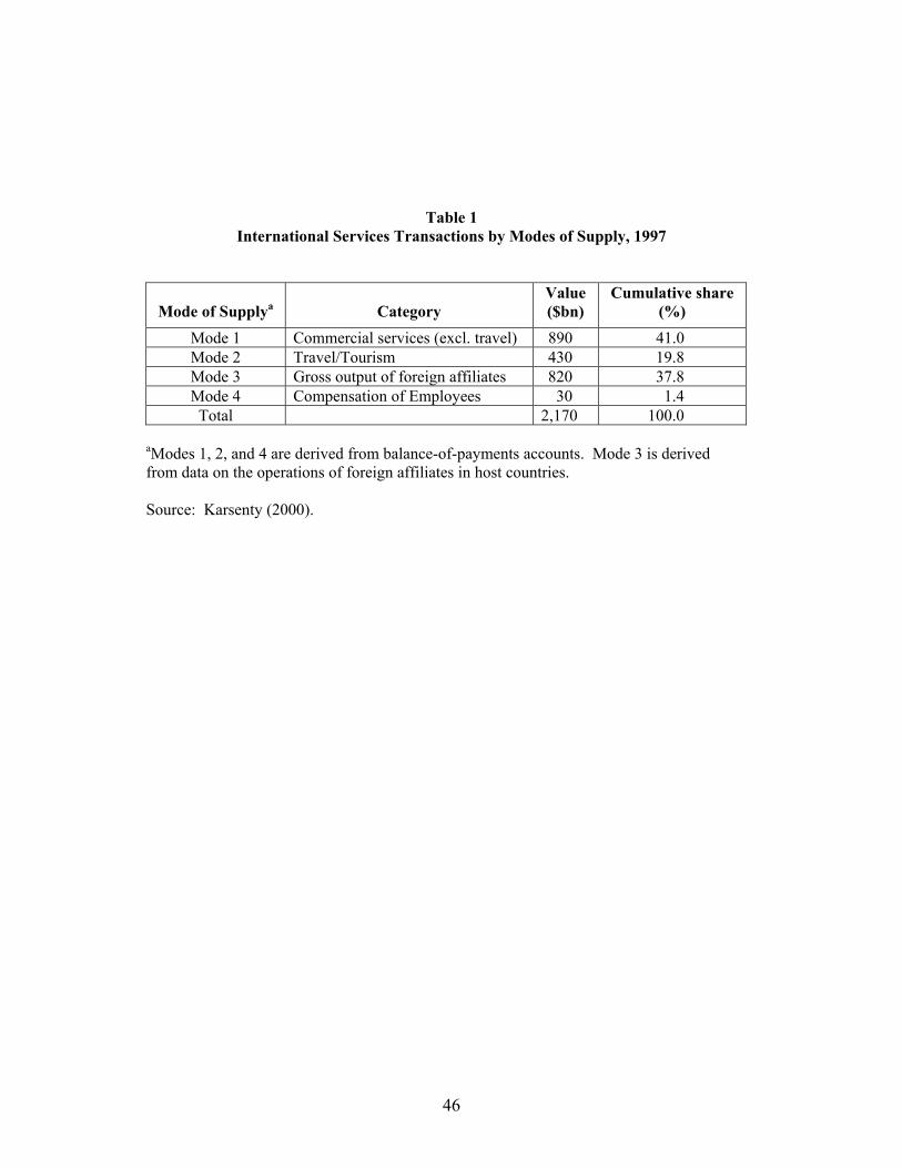
46

Table 1 International Services Transactions by Modes of Supply, 1997

Mode of Supplya

Category

Value ($bn)

Cumulative share (%)

Mode 1 Commercial services (excl. travel) 890 41.0 Mode 2 Travel/Tourism 430 19.8 Mode 3 Gross output of foreign affiliates 820 37.8 Mode 4 Compensation of Employees 30 1.4 Total 2,170 100.0

aModes 1, 2, and 4 are derived from balance-of-payments accounts. Mode 3 is derived from data on the operations of foreign affiliates in host countries. Source: Karsenty (2000).

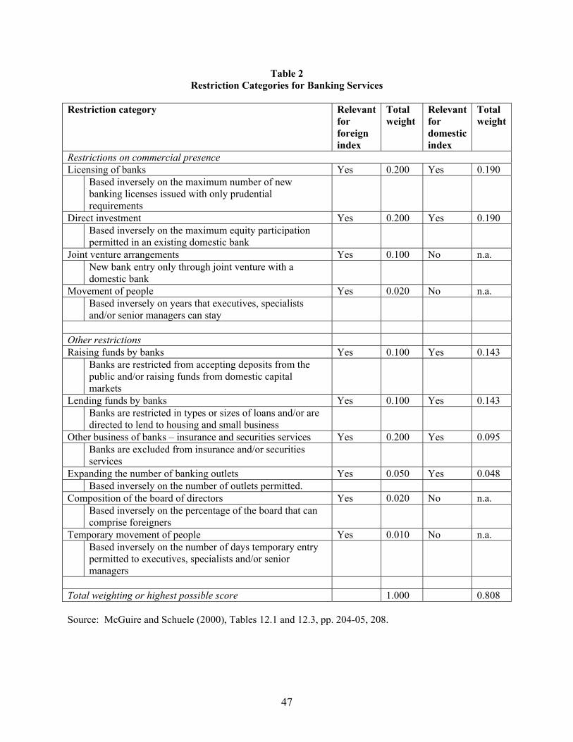
47

Table 2 Restriction Categories for Banking Services

Restriction category Relevant

for foreign index

Total weight

Relevant for domestic index

Total weight

Restrictions on commercial presence Licensing of banks Yes 0.200 Yes 0.190 Based inversely on the maximum number of new

banking licenses issued with only prudential requirements

Direct investment Yes 0.200 Yes 0.190 Based inversely on the maximum equity participation

permitted in an existing domestic bank

Joint venture arrangements Yes 0.100 No n.a. New bank entry only through joint venture with a

domestic bank

Movement of people Yes 0.020 No n.a. Based inversely on years that executives, specialists

and/or senior managers can stay

Other restrictions Raising funds by banks Yes 0.100 Yes 0.143 Banks are restricted from accepting deposits from the

public and/or raising funds from domestic capital markets

Lending funds by banks Yes 0.100 Yes 0.143 Banks are restricted in types or sizes of loans and/or are

directed to lend to housing and small business

Other business of banks – insurance and securities services Yes 0.200 Yes 0.095 Banks are excluded from insurance and/or securities

services

Expanding the number of banking outlets Yes 0.050 Yes 0.048 Based inversely on the number of outlets permitted. Composition of the board of directors Yes 0.020 No n.a. Based inversely on the percentage of the board that can

comprise foreigners

Temporary movement of people Yes 0.010 No n.a. Based inversely on the number of days temporary entry

permitted to executives, specialists and/or senior managers

Total weighting or highest possible score 1.000 0.808 Source: McGuire and Schuele (2000), Tables 12.1 and 12.3, pp. 204-05, 208.

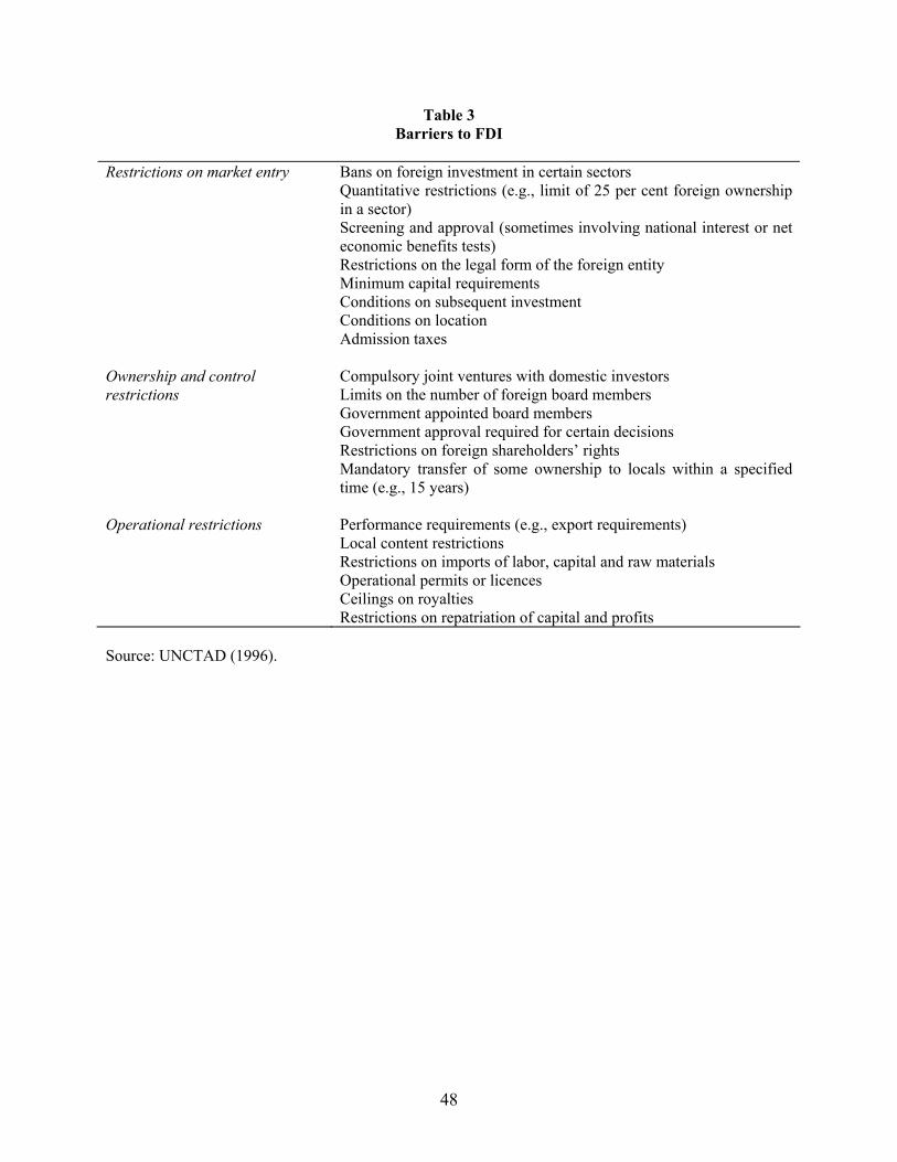
48

Table 3 Barriers to FDI

Restrictions on market entry Bans on foreign investment in certain sectors Quantitative restrictions (e.g., limit of 25 per cent foreign ownership

in a sector) Screening and approval (sometimes involving national interest or net

economic benefits tests) Restrictions on the legal form of the foreign entity Minimum capital requirements Conditions on subsequent investment Conditions on location Admission taxes Ownership and control Compulsory joint ventures with domestic investors restrictions Limits on the number of foreign board members Government appointed board members Government approval required for certain decisions Restrictions on foreign shareholders’ rights Mandatory transfer of some ownership to locals within a specified

time (e.g., 15 years) Operational restrictions Performance requirements (e.g., export requirements) Local content restrictions Restrictions on imports of labor, capital and raw materials Operational permits or licences Ceilings on royalties Restrictions on repatriation of capital and profits Source: UNCTAD (1996).

49

Table 4 Components of an Index of FDI Restrictions

Type of restriction Weight Foreign equity limits on all firms

No foreign equity permitted 1.000 Less than 50 per cent foreign equity permitted 0.500 More than 50 per cent and less than 100 per cent foreign equity permitted 0.250

Foreign equity limits on existing firms, none on greenfield

No foreign equity permitted 0.500 Less than 50 per cent foreign equity permitted 0.250 More than 50 per cent and less than 100 per cent foreign equity permitted 0.125

Screening and approval

Investor required to demonstrate net economic benefits 0.100 Approval unless contrary to national interest 0.075 Notification (pre or post) 0.050

Control and management restrictions

All firms 0.200 Existing firms, none for greenfield 0.100

Input and operational restrictions

All firms 0.200 Existing firms, none for greenfield 0.100

Source: Holmes and Hardin (2000, p. 62).

50

Table 5 FDI Restrictiveness Indexes for Selected APEC Economies and Selected Sectors, 1996-98 (Percentage)

Sectors Australia Canada China Hong Kong Indonesia Japan Korea Malaysia Business 0.183 0.225 0.360 0.015 0.560 0.062 0.565 0.316 Communications 0.443 0.514 0.819 0.350 0.644 0.350 0.685 0.416 Postal 1.000 1.000 1.000 1.000 1.000 1.000 1.000 1.000 Courier 0.175 0.200 0.275 0.000 0.525 0.050 0.550 0.075 Telecommunications 0.300 0.325 1.000 0.200 0.525 0.100 0.550 0.375 Audiovisual 0.295 0.530 1.000 0.200 0.525 0.250 0.640 0.215 Construction 0.175 0.200 0.400 0.000 0.525 0.050 0.750 0.775 Distribution 0.175 0.200 0.275 0.050 0.525 0.050 0.625 0.075 Education 0.175 0.200 0.525 0.000 0.525 0.200 0.550 0.075 Environmental 0.175 0.200 0.275 0.000 0.525 0.117 0.700 0.075 Financial 0.450 0.375 0.450 0.233 0.550 0.358 0.875 0.608 Insurance and related 0.275 0.425 0.475 0.400 0.575 0.450 0.838 0.600 Banking and other 0.625 0.325 0.425 0.067 0.525 0.267 0.913 0.617 Health 0.175 0.200 0.275 0.000 0.525 0.050 0.550 0.317 Tourism 0.175 0.200 0.283 0.000 0.525 0.050 0.617 0.542 Recreation 0.175 0.200 0.275 0.000 0.525 0.050 0.550 0.175 Transport 0.204 0.235 0.455 0.093 0.525 0.114 0.573 0.122

Mexico New Zealand Papua New Guinea Philippines Singapore Thailand United States Business 0.289 0.086 0.300 0.479 0.261 0.775 0.005 Communications 0.739 0.434 0.475 0.758 0.518 0.838 0.345 Postal 1.000 1.000 1.000 1.000 1.000 1.000 1.000 Courier 0.775 0.075 0.300 0.475 0.250 0.775 0.000 Telecommunications 0.705 0.425 0.300 0.975 0.571 0.804 0.200 Audiovisual 0.475 0.235 0.300 0.580 0.250 0.775 0.180 Construction 0.450 0.075 0.300 0.475 0.250 0.775 0.000 Distribution 0.325 0.075 0.300 0.475 0.250 0.775 0.000 Education 0.450 0.075 0.300 0.475 0.250 0.775 0.000 Environmental 0.075 0.075 0.300 0.475 0.250 0.775 0.000 Financial 0.554 0.200 0.300 0.954 0.378 0.875 0.200 Insurance and related 0.575 0.125 0.300 0.975 0.250 0.775 0.000 Banking and other 0.533 0.275 0.300 0.933 0.506 0.975 0.400 Health 0.408 0.075 0.300 0.475 0.250 0.775 0.000 Tourism 0.275 0.075 0.300 0.808 0.317 0.775 0.000 Recreational 0.075 0.075 0.300 0.475 0.250 0.775 0.000 Transport 0.283 0.131 0.300 0.975 0.250 0.780 0.025

Note: The higher the score, the greater the degree to which an industry is restricted. The maximum score is 100%. Because of data constraints on the value of output by sector, the indexes shown are based on simple averages of the sub-sectors involved in the individual countries. Source: Adapted from Holmes and Hardin (2000, pp. 63-64).

51

Table 6 Constructed Ad Valorem Tariff Equivalent “Guesstimates” by 1-Digit ISIC Services

Sectors for Selected Countries (Percentage)

Country

ISIC 5 Con-

struction

ISIC 6

Wholesale & Retail Distr.

ISIC 7 Transp.,

Storage & Communic.

ISIC 8

Business & Fin. Services

ISIC 9 Social & Personal Services

Australia 12.0 7.4 183.4 24.8 25.4 Austria 5.0 4.6 98.7 20.1 13.9 Canada 6.0 9.0 117.7 25.9 40.2 Chile 40.0 34.4 182.2 45.2 42.9 European Union

10.0 10.0 182.0 27.2 23.6

Finland 19.0 14.6 181.0 23.8 31.7 Hong Kong 32.0 31.5 149.8 39.0 42.9 Japan 5.0 4.6 142.0 28.9 32.3 Korea 16.0 21.4 164.9 36.3 40.7 Mexico 24.0 21.3 152.3 40.9 29.8 New Zealand 5.0 13.4 181.5 30.5 36.1 Norway 5.0 13.4 122.2 25.7 24.0 Singapore 12.0 34.4 138.8 35.9 33.7 Sweden 12.0 13.4 184.2 22.5 26.9 Switzerland 5.0 8.0 178.1 27.7 32.3 Turkey 5.0 34.4 31.6 35.4 35.9 United States 5.0 4.6 111.4 21.7 31.7

Source: Hoekman (1995, pp. 355-56).

52

Table 7 International Air Passenger Transport: Bilateral Restriction Indexes and Price Impacts

Price Impactsb

Number of Agreements

/Routes

Bilateral Restriction

Indexa Business Economy Discount Asia Pacific economies Australia 24 0.62 146.0 54.8 14.6 India 20 0.77 164.4 81.3 21.8 Indonesia 16 0.73 139.7 53.0 20.4 Japan 29 0.73 121.1 41.4 18.1 Korea 18 0.72 181.5 89.9 20.4 Malaysia 22 0.71 199.1 95.6 18.4 New Zealand 15 0.39 82.1 66.8 11.7 Philippines 20 0.79 207.5 70.1 20.9 Singapore 30 0.70 141.5 57.5 16.8 Thailand 25 0.68 124.5 71.3 16.2 Americas economies Argentina 12 0.74 161.7 62.0 17.5 Brazil 19 0.70 195.5 63.9 15.5 Canada 29 0.60 114.5 56.9 11.4 Chile 17 0.61 125.2 49.5 12.9 Mexico 19 0.82 224.7 92.2 18.4 Uruguay 32 0.52 96.9 38.5 12.3 USA 32 0.40 52.9 33.2 8.9 European economies Austria 28 0.32 47.2 20.6 6.1 Belgium 31 0.36 63.3 22.0 6.9 Denmark 30 0.34 53.1 21.1 7.0 Finland 22 0.23 33.6 11.5 3.8 France 32 0.35 57.0 20.8 8.3 Germany 32 0.37 56.5 20.3 8.1 Greece 26 0.31 72.1 24.9 7.2 Ireland 23 0.21 32.2 20.1 4.5 Italy 25 0.29 49.9 18.5 6.4 Luxembourg 23 0.24 36.9 15.0 4.2 Netherlands 31 0.39 104.0 20.0 10.0 Norway 28 0.32 62.1 16.4 4.4 Portugal 21 0.14 45.5 20.3 6.1 Spain 31 0.36 68.0 25.4 8.9 Sweden 29 0.32 45.5 20.3 6.1 Switzerland 32 0.75 102.5 42.6 13.8 Turkey 20 0.56 98.8 32.2 10.7 United Kingdom 32 0.30 46.3 21.5 7.6

a Unweighted average of the route-level bilateral restriction indexes for each economy based on the number of agreements/routes shown in the preceding column. Ranges from 0 to 0.97, with a higher score indicating more restrictions.

b Percentage increase in airfares compared to the benchmark regime. Source: Doove et al. (2001, p. 39).

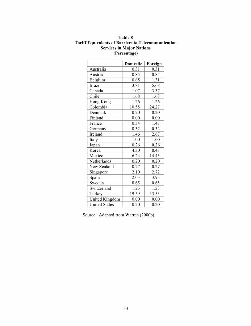
53

Table 8

Tariff Equivalents of Barriers to Telecommunication Services in Major Nations

(Percentage)

Domestic ForeignAustralia 0.31 0.31 Austria 0.85 0.85 Belgium 0.65 1.31 Brazil 3.81 5.68 Canada 1.07 3.37 Chile 1.68 1.68 Hong Kong 1.26 1.26 Colombia 10.55 24.27 Denmark 0.20 0.20 Finland 0.00 0.00 France 0.34 1.43 Germany 0.32 0.32 Ireland 1.46 2.67 Italy 1.00 1.00 Japan 0.26 0.26 Korea 4.30 8.43 Mexico 6.24 14.43 Netherlands 0.20 0.20 New Zealand 0.27 0.27 Singapore 2.10 2.72 Spain 2.03 3.93 Sweden 0.65 0.65 Switzerland 1.23 1.23 Turkey 19.59 33.53 United Kingdom 0.00 0.00 United States 0.20 0.20

Source: Adapted from Warren (2000b).

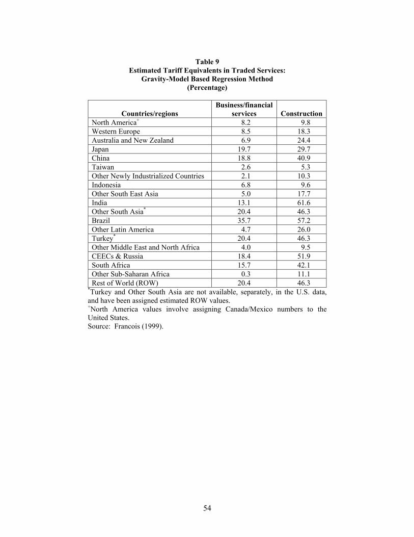
54

Table 9

Estimated Tariff Equivalents in Traded Services: Gravity-Model Based Regression Method

(Percentage)

Countries/regions

Business/financialservices

Construction

North America+ 8.2 9.8 Western Europe 8.5 18.3 Australia and New Zealand 6.9 24.4 Japan 19.7 29.7 China 18.8 40.9 Taiwan 2.6 5.3 Other Newly Industrialized Countries 2.1 10.3 Indonesia 6.8 9.6 Other South East Asia 5.0 17.7 India 13.1 61.6 Other South Asia* 20.4 46.3 Brazil 35.7 57.2 Other Latin America 4.7 26.0 Turkey* 20.4 46.3 Other Middle East and North Africa 4.0 9.5 CEECs & Russia 18.4 51.9 South Africa 15.7 42.1 Other Sub-Saharan Africa 0.3 11.1 Rest of World (ROW) 20.4 46.3

*Turkey and Other South Asia are not available, separately, in the U.S. data, and have been assigned estimated ROW values. +North America values involve assigning Canada/Mexico numbers to the United States. Source: Francois (1999).

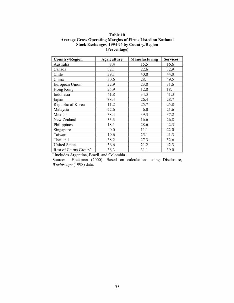
55

Table 10

Average Gross Operating Margins of Firms Listed on National Stock Exchanges, 1994-96 by Country/Region

(Percentage)

Country/Region Agriculture Manufacturing Services Australia 8.4 15.5 16.6 Canada 32.1 22.6 32.9 Chile 39.1 40.8 44.0 China 30.6 28.1 49.5 European Union 22.9 23.8 31.6 Hong Kong 25.9 12.8 18.1 Indonesia 41.8 34.3 41.3 Japan 38.4 26.4 28.7 Republic of Korea 11.2 25.7 25.8 Malaysia 22.6 6.0 21.6 Mexico 38.4 39.3 37.2 New Zealand 33.3 16.6 26.8 Philippines 18.1 28.6 42.3 Singapore 0.0 11.1 22.0 Taiwan 19.6 25.1 41.3 Thailand 38.2 27.3 52.6 United States 36.6 21.2 42.3 Rest of Cairns Groupa 36.3 31.1 39.0

a Includes Argentina, Brazil, and Colombia. Source: Hoekman (2000). Based on calculations using Disclosure, Worldscope (1998) data.

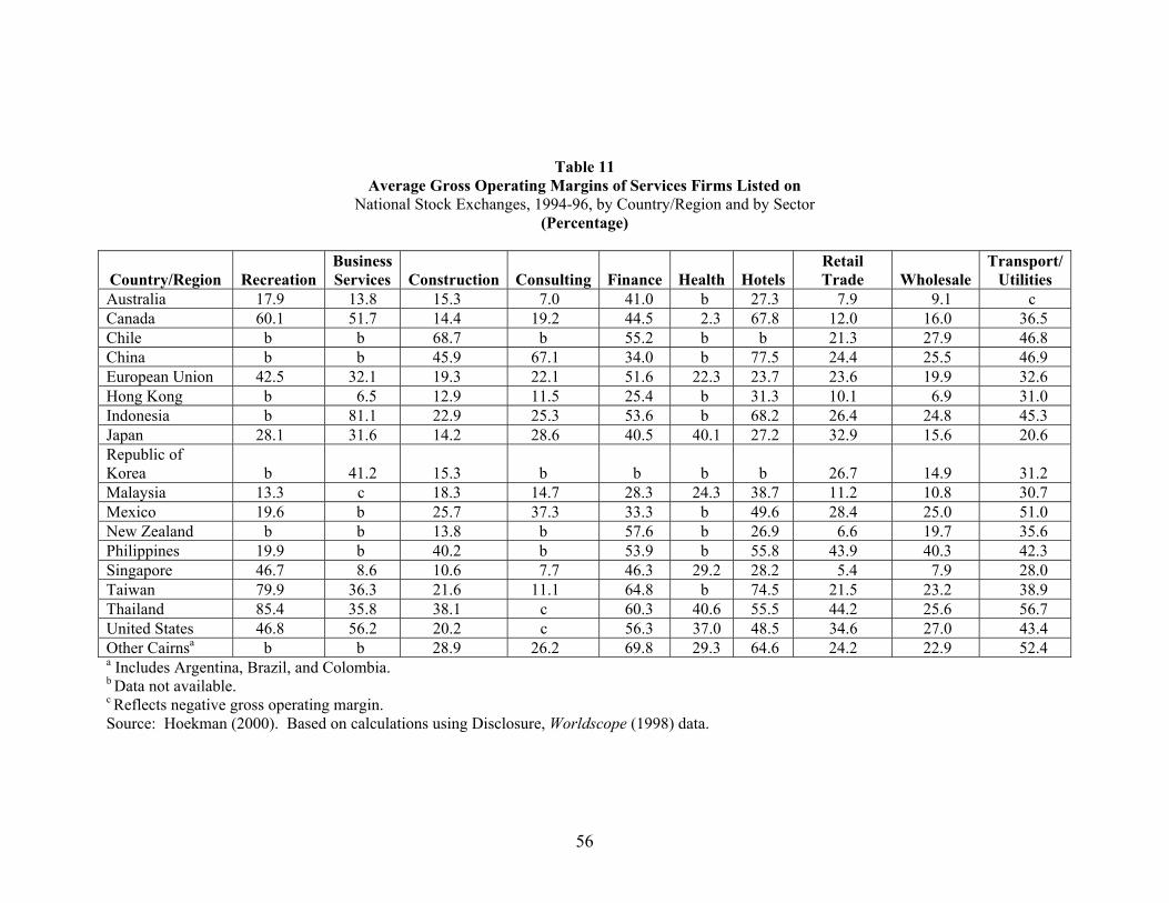
56

Table 11

Average Gross Operating Margins of Services Firms Listed on National Stock Exchanges, 1994-96, by Country/Region and by Sector

(Percentage)

Country/Region Recreation BusinessServices Construction Consulting Finance Health Hotels

Retail Trade Wholesale

Transport/Utilities

Australia 17.9 13.8 15.3 7.0 41.0 b 27.3 7.9 9.1 c

Canada 60.1 51.7 14.4 19.2 44.5 2.3 67.8 12.0 16.0 36.5 Chile b b 68.7 b 55.2 b b 21.3 27.9 46.8 China b b 45.9 67.1 34.0 b 77.5 24.4 25.5 46.9 European Union 42.5 32.1 19.3 22.1 51.6 22.3 23.7 23.6 19.9 32.6 Hong Kong b 6.5 12.9 11.5 25.4 b 31.3 10.1 6.9 31.0 Indonesia b 81.1 22.9 25.3 53.6 b 68.2 26.4 24.8 45.3 Japan 28.1 31.6 14.2 28.6 40.5 40.1 27.2 32.9 15.6 20.6 Republic of Korea b 41.2 15.3 b b b b 26.7 14.9 31.2 Malaysia 13.3 c 18.3 14.7 28.3 24.3 38.7 11.2 10.8 30.7 Mexico 19.6 b 25.7 37.3 33.3 b 49.6 28.4 25.0 51.0 New Zealand b b 13.8 b 57.6 b 26.9 6.6 19.7 35.6 Philippines 19.9 b 40.2 b 53.9 b 55.8 43.9 40.3 42.3 Singapore 46.7 8.6 10.6 7.7 46.3 29.2 28.2 5.4 7.9 28.0 Taiwan 79.9 36.3 21.6 11.1 64.8 b 74.5 21.5 23.2 38.9 Thailand 85.4 35.8 38.1 c 60.3 40.6 55.5 44.2 25.6 56.7 United States 46.8 56.2 20.2 c 56.3 37.0 48.5 34.6 27.0 43.4 Other Cairnsa b b 28.9 26.2 69.8 29.3 64.6 24.2 22.9 52.4 a Includes Argentina, Brazil, and Colombia. b Data not available. c Reflects negative gross operating margin. Source: Hoekman (2000). Based on calculations using Disclosure, Worldscope (1998) data.

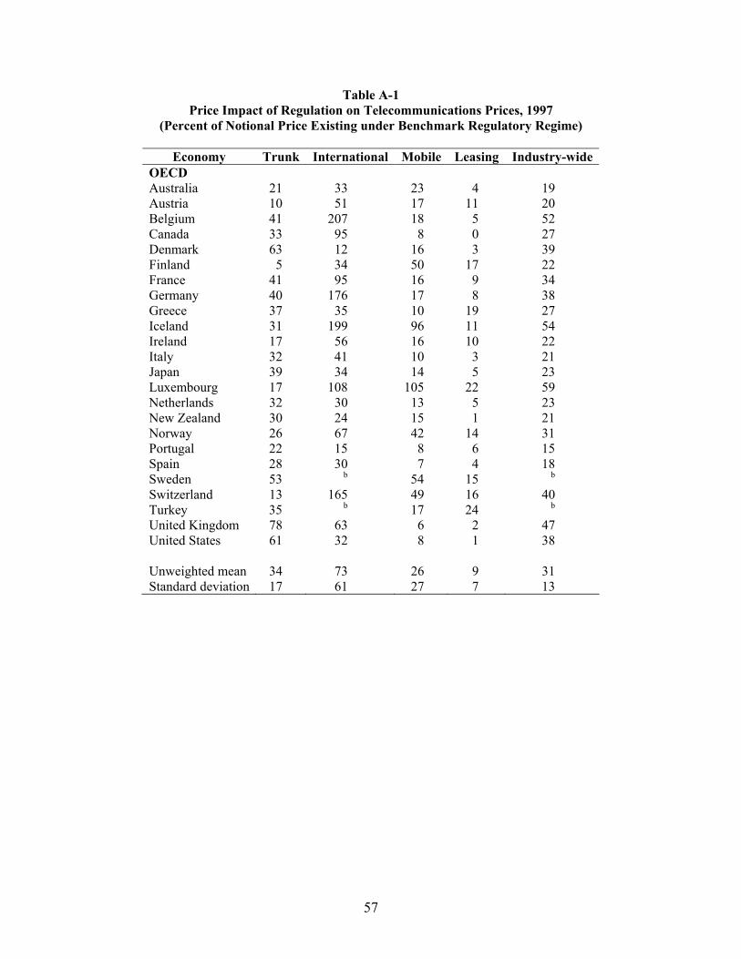
57

Table A-1 Price Impact of Regulation on Telecommunications Prices, 1997

(Percent of Notional Price Existing under Benchmark Regulatory Regime)

Economy Trunk International Mobile Leasing Industry-wide OECD Australia 21 33 23 4 19 Austria 10 51 17 11 20 Belgium 41 207 18 5 52 Canada 33 95 8 0 27 Denmark 63 12 16 3 39 Finland 5 34 50 17 22 France 41 95 16 9 34 Germany 40 176 17 8 38 Greece 37 35 10 19 27 Iceland 31 199 96 11 54 Ireland 17 56 16 10 22 Italy 32 41 10 3 21 Japan 39 34 14 5 23 Luxembourg 17 108 105 22 59 Netherlands 32 30 13 5 23 New Zealand 30 24 15 1 21 Norway 26 67 42 14 31 Portugal 22 15 8 6 15 Spain 28 30 7 4 18 Sweden 53 b 54 15 b

Switzerland 13 165 49 16 40 Turkey 35 b 17 24 b

United Kingdom 78 63 6 2 47 United States 61 32 8 1 38 Unweighted mean 34 73 26 9 31 Standard deviation 17 61 27 7 13

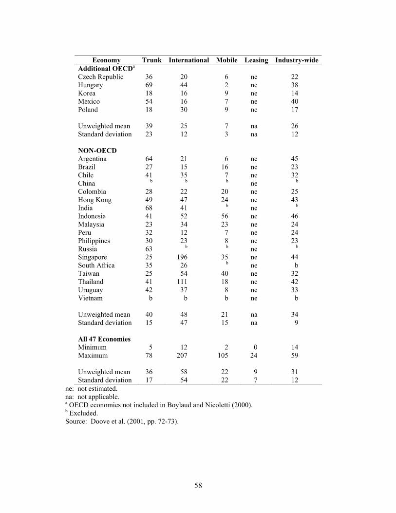
58

Economy Trunk International Mobile Leasing Industry-wide

Additional OECDa Czech Republic 36 20 6 ne 22 Hungary 69 44 2 ne 38 Korea 18 16 9 ne 14 Mexico 54 16 7 ne 40 Poland 18 30 9 ne 17 Unweighted mean 39 25 7 na 26 Standard deviation 23 12 3 na 12 NON-OECD Argentina 64 21 6 ne 45 Brazil 27 15 16 ne 23 Chile 41 35 7 ne 32 China b b b ne b

Colombia 28 22 20 ne 25 Hong Kong 49 47 24 ne 43 India 68 41 b ne b

Indonesia 41 52 56 ne 46 Malaysia 23 34 23 ne 24 Peru 32 12 7 ne 24 Philippines 30 23 8 ne 23 Russia 63 b b ne b

Singapore 25 196 35 ne 44 South Africa 35 26 b ne b Taiwan 25 54 40 ne 32 Thailand 41 111 18 ne 42 Uruguay 42 37 8 ne 33 Vietnam b b b ne b Unweighted mean 40 48 21 na 34 Standard deviation 15 47 15 na 9 All 47 Economies Minimum 5 12 2 0 14 Maximum 78 207 105 24 59 Unweighted mean 36 58 22 9 31 Standard deviation 17 54 22 7 12

ne: not estimated. na: not applicable. a OECD economies not included in Boylaud and Nicoletti (2000). b Excluded. Source: Doove et al. (2001, pp. 72-73).

59

Table A-2 Price Impacts of Regulation on Industrial Electricity Prices, 1996a

Economies in Original Study Percent Extended Coverage Percent Australia 0.0 Argentina 0.0 Belgium 15.4 Austria 13.2 Canada 8.8 Bolivia 16.5 Denmark 8.5 Brazil 15.6 Finland 0.0 Chile 0.0 France 16.0 China 17.2 Germany 8.3 Colombia 0.0 Greece 16.6 Czech Republic 13.6 Ireland 13.9 Hong Kong 15.6 Italy 17.1 Hungary 13.3 Japan 10.2 Iceland 35.3 Netherlands 15.5 India 17.2 New Zealand 0.0 Indonesia 16.8 Norway 0.0 Korea 15.4 Portugal 17.9 Luxembourg 13.8 Spain 9.5 Malaysia 16.6 Sweden 0.0 Mexico 17.3 United Kingdom 0.0 Peru 0.0 United States 7.5 Philippines 17.6 Poland 13.6 Russia 17.1 Slovak Republic 14.8 Singapore 15.6 South Africa 15.6 Switzerland 21.9 Taiwan 16.1 Thailand 16.3 Turkey 20.7 Uruguay 32.2 Venezuela 27.2 Vietnam 32.0

a Percentage increase in pre-tax industrial electricity prices relative to the estimated price under the benchmark regulatory regime. Source: Doove et al. (2001, p. 105).

60

Table A-3 Estimated Cost Impacts of Foreign and Domestic Barriers to Establishment

in Wholesale and Retail Food Distributors (Percent)

Economy Cost Impact of Foreign

Barriers to EstablishmentCost Impact of Domestic

Barriers to Establishment Australia 0.57 - Belgium 4.87 6.69 Canada 3.09 0.98 Chile 1.32 1.92 France 5.16 7.10 Greece 0.25 - Hong Kong 0.06 - Indonesia 3.66 - Ireland 2.70 - Japan 2.26 6.79 Malaysia 8.23 3.97 Netherlands 2.73 - New Zealand 0.77 - Singapore 0.03 - South Africa 0.47 - Switzerland 5.24 8.32 United Kingdom 2.76 - United States 2.26 -

- Zero. Source: Kalirajan (2000, p. 52).

61

Table A-4

Estimated Price Impacts of Foreign and Domestic Trade Restrictiveness Indexes (TRI) on Net Interest Margins of Banks

(Percent)

Economy Price Effect Usingthe Foreign TRIi

Price Effect Using the Domestic TRIi

b Argentina 5.34 0.00 Australia 9.30 0.00 Canada 5.34 0.00 Chile 34.00 23.67 Colombia 18.35 3.73 European Uniona 5.32 0.00 Hong Kong 6.91 2.97 Indonesia 49.32 5.26 Japan 15.26 9.99 Malaysia 60.61 21.86 Philippines 47.36 10.79 Singapore 31.45 8.39 South Korea 36.72 14.93 Switzerland 5.95 0.00 Thailand 33.06 0.00 United States 4.75 0.00

a The European Union grouping excludes Finland, Ireland and Luxembourg. b Uses the coefficient estimate for the foreign trade restrictiveness index as a proxy. Source: Kalirajan et al. (2000, p. 229).

62

Table A-5

Estimated Price and Cost Impacts of Restrictions on Engineering Services (Percent)

Price Impact Cost Impact

Foreign Barriers

to Establishment

Foreign Barriers to Ongoing Operations

All Foreign Barriers

Domestic Barriers toEstablishment

Austria 11.1 3.5 14.5 6.8 Mexico 13.9 0.2 14.2 1.9 Malaysia 11.3 0.7 12.0 5.3 Indonesia 9.9 0.3 10.2 3.2 Germany 4.7 5.5 10.2 2.9 Spain 5.1 3.7 8.7 3.9 United States 5.1 2.2 7.4 3.8 Sweden 5.9 0.9 6.8 0.7 Japan 3.1 3.4 6.6 2.2 Canada 3.1 2.2 5.3 2.7 Singapore 4.9 0.2 5.0 0.8 Hong Kong 3.6 1.5 5.1 2.3 South Africa 3.5 0.2 3.7 0.7 Netherlands 3.5 0.2 3.7 5.2 Australia 2.1 0.7 2.8 2.1 United Kingdom 2.3 0.2 2.5 1.4 Finland 1.8 0.5 2.3 0.7 Denmark 0.3 0.8 1.1 0.7 France 0.3 0.6 0.9 0.7 Belgium 0.3 0.2 0.5 0.7 a The price impact for all foreign barriers is the sum of the price impacts for foreign barriers to establishment and ongoing operations, respectively. Source: Nguyen-Hong (2000, p. 63).

63

Table A-6

Coefficient Estimates of Technical Efficiency in Telecommunications Services

Low Income Technical Efficiency High Income Technical Efficiency Chile 3.82 Australia 1.67 China 6.31 Austria 1.31 Hungary 2.61 Belgium 1.55 Iceland 1.16 Canada 1.34 Indonesia 11.96 Denmark 1.43 Ireland 3.22 Finland 1.24 Malaysia 4.31 France 1.74 Mexico 15.41 Germany 1.66 PNG 7.75 Greece 1.11 Philippines 3.06 Hong Kong 1.44 Poland 2.30 Italy 1.71 Thailand 5.25 Japan 1.21 Turkey 4.07 Korea 1.98 Luxembourg 1.03 Netherlands 1.43 New Zealand 1.83 Norway 1.75 Portugal 2.08 Singapore 1.57 Spain 1.75 Sweden 1.40 Switzerland 1.42 United Kingdom 1.67 United States 1.48 Mean 5.48 Mean 1.54

Note: A coefficient estimate equal to 1.00 indicates full technical efficiency in relation to the minimum-cost frontier. Source: Trewin (2000, p. 112).

64

Table A-7 Welfare Effects of Elimination of Services

(Percent and Billions of Dollars)

Country

Scenario A Perfect Int’l Capital Mobility and Fixed

World Capital Stock

Scenario B Risk-Premium

Elasticity=0.1 and Fixed World Capital Stock

Scenario C Risk-Premium

Elasticity=0.1 and World Capital Stock Increased by

3% Industrialized

Countries % GNP $Bill. % GNP $Bill. % GNP $Bill. Australia 1.8 6.0 1.5 5.0 4.9 16.8 Canada 14.8 84.0 12.9 73.7 14.9 85.0 European Union 0.5 42.4 0.5 38.0 2.5 202.4 Japan -2.0 -103.7 -1.7 -88.4 0.5 25.7 New Zealand 9.1 5.2 7.5 4.3 10.5 6.0 United States 0.5 35.0 0.3 23.2 3.1 222.5

Developing Countries

Asia China 3.8 26.9 3.2 22.9 6.0 42.8 Hong Kong 6.6 6.6 5.4 5.5 13.4 13.5 Indonesia 15.6 30.8 13.1 25.8 16.9 33.3 Korea -2.8 -12.3 -2.3 -10.1 1.4 6.4 Malaysia 2.3 2.1 1.9 1.8 4.7 4.4 Philippines 2.3 1.6 1.9 1.3 8.3 5.7 Singapore 1.7 1.0 1.3 0.7 4.3 2.5 Taiwan 7.6 20.7 6.8 18.5 7.7 21.2 Thailand -2.2 -3.6 -1.8 -2.9 4.4 7.1

Other

Chile -2.0 -1.3 -1.6 -1.0 2.7 1.7 Mexico -4.3 -11.7 -3.2 -8.8 0.2 0.5 Rest of Cairns -3.7 -39.6 -3.2 -34.1 0.6 6.2

Total 90.3 75.6 703.7 Source: Brown and Stern (2001, pp. 277-78).

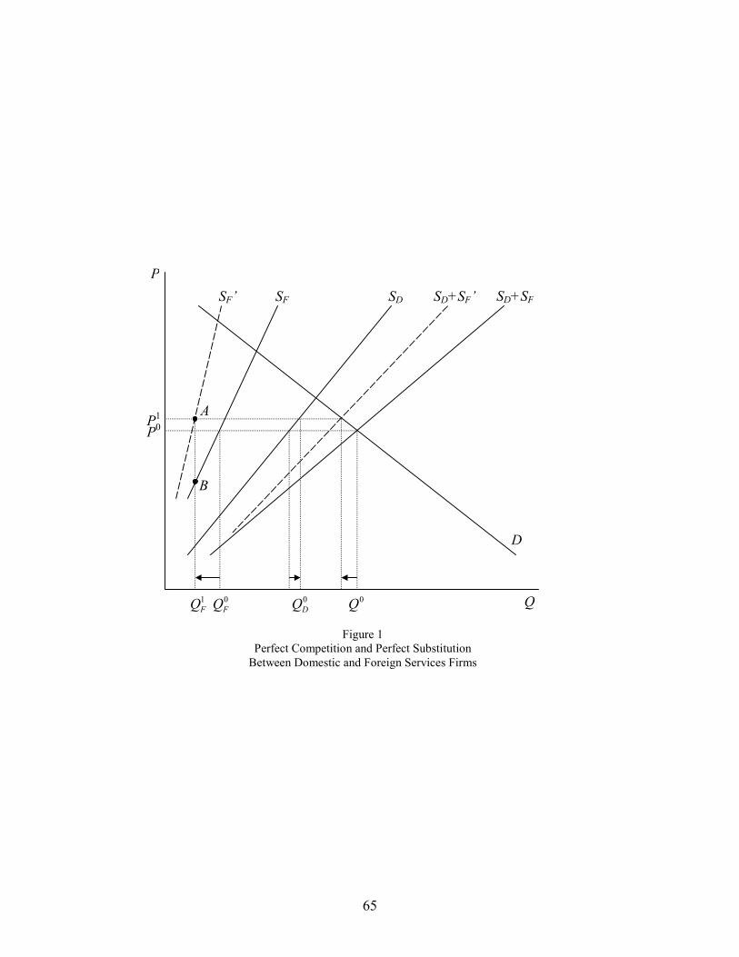
65

Q

P

D

SF SF’ SD SD+SF SD+SF’

P0 P1

B

A

Figure 1 Perfect Competition and Perfect Substitution

Between Domestic and Foreign Services Firms

0FQ 0

DQ 0Q 1FQ

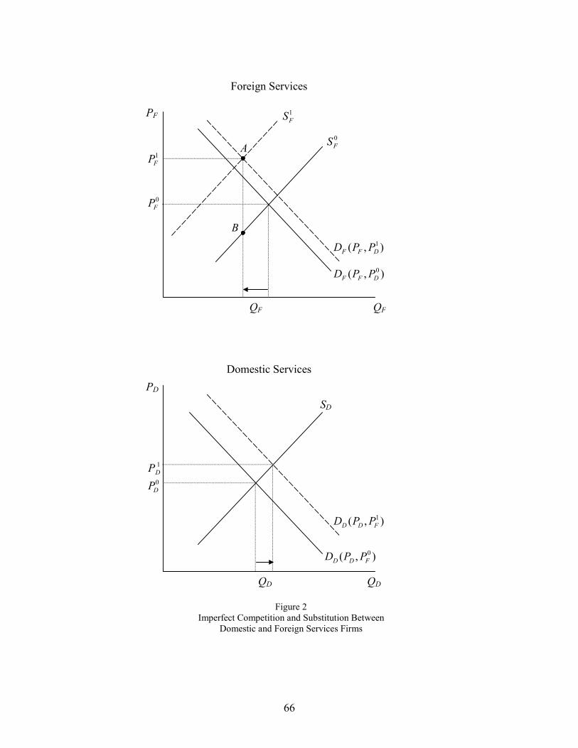
66

QF

PF

Figure 2 Imperfect Competition and Substitution Between

Domestic and Foreign Services Firms

),( 0FDD PPD

PD

Domestic Services

Foreign Services

),( 1FDD PPD

QD

SD

0DP

1DP

QD

),( 0DFF PPD

),( 1DFF PPD

0FP

1FP

A

B

QF

1FS

0FS

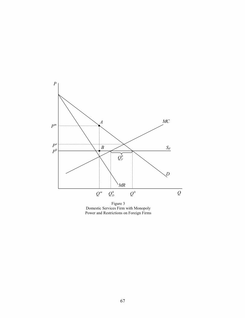
67

Q

P

Figure 3 Domestic Services Firm with Monopoly Power and Restrictions on Foreign Firms

D

SF

MC

MR

0DQ 0Q mQ

P0 Pa

Pm A

B

0FQ

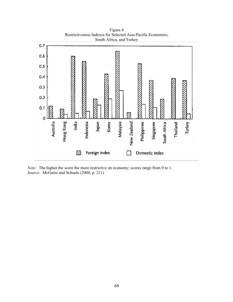
68

Figure 4 Restrictiveness Indexes for Selected Asia-Pacific Economies,

South Africa, and Turkey

Note: The higher the score the more restrictive an economy; scores range from 0 to 1. Source: McGuire and Schuele (2000, p. 211)

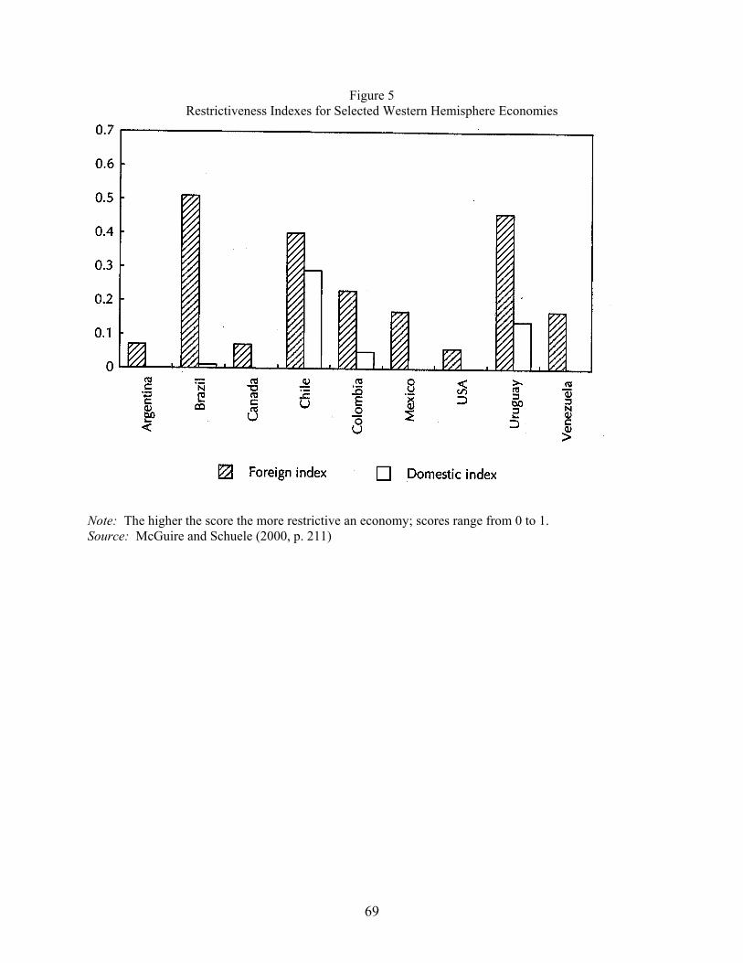
69

Figure 5 Restrictiveness Indexes for Selected Western Hemisphere Economies

Note: The higher the score the more restrictive an economy; scores range from 0 to 1. Source: McGuire and Schuele (2000, p. 211)

70

Appendix B

Study Questions and Exercises B-1: Study Questions

I. Introduction

1. What is the difference between a tariff and nontariff barrier (NTB)?

2. What is a tariff equivalent, and how is it measured?

3. What are the four modes of supply of traded services? To what extent can barriers to traded services be measured as tariff equivalents?

4. What are “frequency measures” of barriers to trade in services? Price and/or quantity

measurements?

II. Conceptual Framework

1. How can the demand and supply of services be depicted under conditions of competition and perfect substitution? What is the effect of an impediment to the foreign supply of services and the determination of the tariff equivalent of the impediment?

2. What are the effects when the services provided are imperfect substitutes? What are the

effects when there are impediments to entry of firms?

III. Characteristics of Services Barriers

1. Why are services barriers more akin to NTBs than tariffs?

2. What are the two dimensions of the government regulation of services, and how may the supply curve for services be affected?

3. In the case of banking services, what are the principal foreign and domestic services

restrictions that may be present, and how may the different degrees of restriction be scored and weighted? How can the discrimination against foreign banks be measured? What is an “index of restrictiveness,” and how is it calculated?

4. What are the main types and most prevalent characteristics of barriers to FDI in services?

IV. Methods of Measurement of Services Barriers

Frequency Studies and Indexes of Restrictiveness 1. What are direct and indirect measurements of barriers to trade in goods and services?

How may price comparisons be used?

2. What are the steps involved in carrying out frequency studies and constructing indexes of restrictiveness for specific services sectors or across multiple sectors? How are indexes of restrictiveness scored, weighted, and used in assessing economic performance?

71

3. How may commitments in the GATS be used in constructing frequency measurements

and indexes of restrictiveness? What is the “positive list” approach? What are the drawbacks of using data on GATS commitments? How are the data on actual FDI restrictions in the APEC countries weighted? Which services sectors appear to be the most subject to FDI restrictions? Which APEC countries?

4. What is the distinction between foreign and domestic restrictiveness indexes? Which

countries appear to have the greatest degree of discrimination against foreign banks?

5. How useful are restrictiveness indexes, and how can they be used in assessing the impacts of services barriers?

Price-Impact and Quantity-Impact Measurements 1. How did Hoekman calculate “guesstimates” of the tariff equivalents of services barriers?

What are the limitations of Hoekman’s methodology?

2. How can restrictiveness indexes be used in econometric estimation of the price effects of the restrictions? What additional information is needed to construct these estimates?

3. How can the quantitative impact of barriers on services trade be calculated and the

associated tariff equivalents?

Gravity-Model Estimates 1. What is a gravity model, and how can it be used to determine the levels of services trade

barriers across countries? What are the advantages and limitations of gravity-model estimates of services barriers?

Financial-Based Measurements 1. What are financial-based measurements, and how can they be used to determine the

levels of services trade barriers across countries? What are the advantages and limitations of these measurements?

V. Measuring the Economic Consequences of Liberalizing Services Barriers

1. What are the three approaches to the CGE modeling of services liberalization?

2. What are the characteristics and assumptions of the Brown and Stern CGE model of

services liberalization? How do they measure services barriers?

3. What are the computational scenarios that Brown and Stern investigate, and what are the results? What are the effects of international capital mobility and an increase in the world’s capital stock?

72

B-2: Exercises

These exercises use the hypothetical data presented in the accompanying tables below, which deal with four products in two industries in three countries. Table B1 describes the restrictions that apply to firms operating in these industries, while tables B2-B5 present data on their domestic and foreign sales, the price prevailing in their domestic markets, the wage rates paid to labor in each industry and country, and national income in each country. Note: Exercises 1 and 2 require no calculation and require instead interpretation of descriptions of restrictions. Exercise 3 requires a minimal amount of calculation, while exercises 4-7 are intended to be more challenging and calculation-intensive, as indicated by asterisks. 1. Which of the restrictions in Table B1 appear to be imposed on the establishment of firms, and which

deal with their operations? Which of the restrictions apply only to foreign firms, and which to all firms?

2. Construct an index of restrictiveness for each product and each country. (You will need to use your own judgment to assign scores to each of the restrictions listed. To maximize the chance that you will assign the same values that appear in the answers, below, limit your scores to 0.0, 0.5, and 1.0. For those industries with two types of restriction, give them equal weight in your index.)

3. Use total sales (domestic plus foreign, from Tables B2 and B3 below) to weight your indexes from question 2 in order to construct restrictiveness indexes for each industry-country pair, and also for each country for the industries combined.

*4. Assuming that the main determinant of prices is the wage rate of labor, use the data in the accompanying tables to estimate (with ordinary least squares, available in spreadsheet programs such as Excel) the following equation:

ijcijciiciijijc rawaap ε+++= 210 lnln

where ijcp is price of product j in industry i, country c, wic is the wage of labor in industry i of

country c, rijc is the restrictiveness index of product j in industry i, country c, and ijcε is a random disturbance. Note that while the wage is assumed to be the same across products within an industry and to have the same effect (in logs) on product prices in the same industry, the intercept of the equation, 0

ija , varies across products.

*5. Use your estimates from question 4 of the price effects of trade barriers to calculate the tariff equivalents that correspond to the restrictiveness indexes in question 2 for each product and country.

*6. Assuming that the main determinant of sales in a country is income, use the data in the accompanying tables to estimate (with ordinary least squares) the following equation:

ijcijciciijijc rbybbs µ+++= 210 lnln

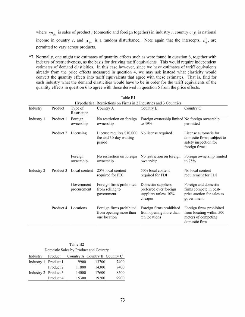
73

where ijcsp is sales of product j (domestic and foreign together) in industry i, country c, yc is national

income in country c, and ijcµ is a random disturbance. Note again that the intercepts, 0ijb , are

permitted to vary across products.

*7. Normally, one might use estimates of quantity effects such as were found in question 6, together with indexes of restrictiveness, as the basis for deriving tariff equivalents. This would require independent estimates of demand elasticities. In this case however, since we have estimates of tariff equivalents already from the price effects measured in question 4, we may ask instead what elasticity would convert the quantity effects into tariff equivalents that agree with these estimates. That is, find for each industry what the demand elasticities would have to be in order for the tariff equivalents of the quantity effects in question 6 to agree with those derived in question 5 from the price effects.

Table B1 Hypothetical Restrictions on Firms in 2 Industries and 3 Countries

Industry Product Type of Restriction

Country A Country B Country C

Industry 1 Product 1 Foreign ownership

No restriction on foreign ownership

Foreign ownership limited to 49%

No foreign ownership permitted

Product 2 Licensing License requires $10,000 fee and 30-day waiting period

No license required License automatic for domestic firms; subject to safety inspection for foreign firms.

Foreign ownership

No restriction on foreign ownership

No restriction on foreign ownership

Foreign ownership limited to 75%

Industry 2 Product 3 Local content 25% local content required for FDI

50% local content required for FDI

No local content requirement for FDI

Government procurement

Foreign firms prohibited from selling to government

Domestic suppliers preferred over foreign suppliers unless 10% cheaper

Foreign and domestic firms compete in best-price auction for sales to government

Product 4 Locations Foreign firms prohibited from opening more than one location

Foreign firms prohibited from opening more than ten locations

Foreign firms prohibited from locating within 500 meters of competing domestic firm

Table B2 Domestic Sales by Product and Country

Industry Product Country A Country B Country C Industry 1 Product 1 9900 13700 7400 Product 2 11800 14300 7400Industry 2 Product 3 14000 17600 8500 Product 4 15300 19200 9900

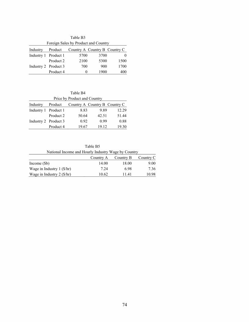
74

Table B3

Foreign Sales by Product and Country Industry Product Country A Country B Country C Industry 1 Product 1 5700 3700 0 Product 2 2100 5300 1500Industry 2 Product 3 700 900 1700 Product 4 0 1900 400

Table B4 Price by Product and Country

Industry Product Country A Country B Country C Industry 1 Product 1 8.83 9.89 12.29 Product 2 50.64 42.51 51.44Industry 2 Product 3 0.92 0.99 0.88 Product 4 19.67 19.12 19.30

Table B5 National Income and Hourly Industry Wage by Country

Country A Country B Country CIncome ($b) 14.00 18.00 9.00Wage in Industry 1 ($/hr) 7.24 6.98 7.36Wage in Industry 2 ($/hr) 10.62 11.41 10.98

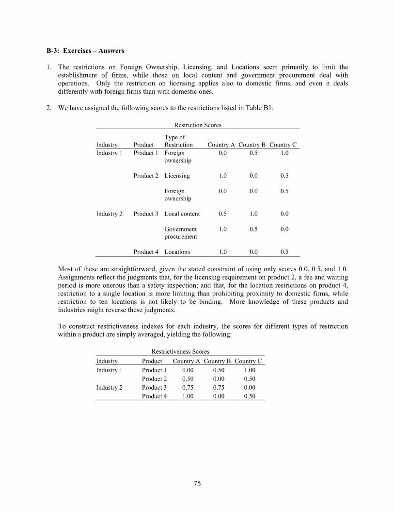
75

B-3: Exercises – Answers 1. The restrictions on Foreign Ownership, Licensing, and Locations seem primarily to limit the

establishment of firms, while those on local content and government procurement deal with operations. Only the restriction on licensing applies also to domestic firms, and even it deals differently with foreign firms than with domestic ones.

2. We have assigned the following scores to the restrictions listed in Table B1:

Restriction Scores

Industry Product Type of Restriction Country A Country B Country C

Industry 1 Product 1 Foreign ownership

0.0 0.5 1.0

Product 2 Licensing

1.0 0.0 0.5

Foreign ownership

0.0 0.0 0.5

Industry 2 Product 3 Local content

0.5 1.0 0.0

Government procurement

1.0 0.5 0.0

Product 4 Locations 1.0 0.0 0.5 Most of these are straightforward, given the stated constraint of using only scores 0.0, 0.5, and 1.0. Assignments reflect the judgments that, for the licensing requirement on product 2, a fee and waiting period is more onerous than a safety inspection; and that, for the location restrictions on product 4, restriction to a single location is more limiting than prohibiting proximity to domestic firms, while restriction to ten locations is not likely to be binding. More knowledge of these products and industries might reverse these judgments. To construct restrictiveness indexes for each industry, the scores for different types of restriction within a product are simply averaged, yielding the following:

Restrictiveness Scores Industry Product Country A Country B Country C Industry 1 Product 1 0.00 0.50 1.00 Product 2 0.50 0.00 0.50 Industry 2 Product 3 0.75 0.75 0.00 Product 4 1.00 0.00 0.50

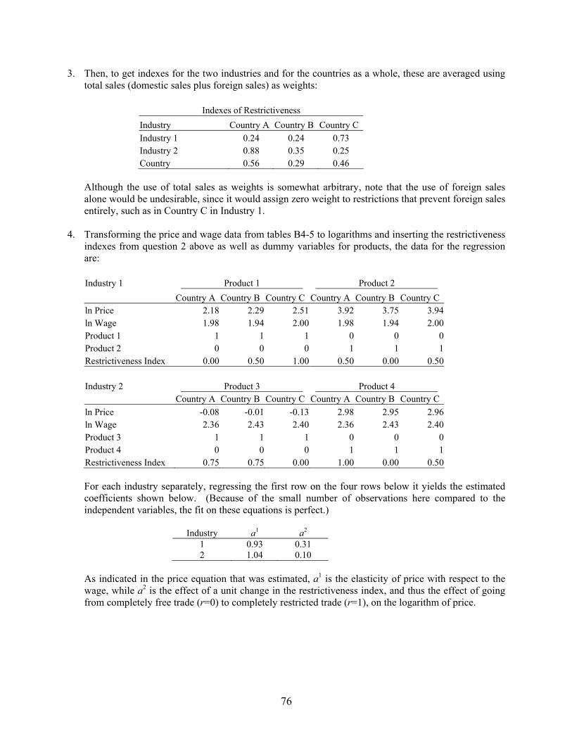
76

3. Then, to get indexes for the two industries and for the countries as a whole, these are averaged using total sales (domestic sales plus foreign sales) as weights:

Indexes of Restrictiveness Industry Country A Country B Country C Industry 1 0.24 0.24 0.73 Industry 2 0.88 0.35 0.25 Country 0.56 0.29 0.46

Although the use of total sales as weights is somewhat arbitrary, note that the use of foreign sales alone would be undesirable, since it would assign zero weight to restrictions that prevent foreign sales entirely, such as in Country C in Industry 1.

4. Transforming the price and wage data from tables B4-5 to logarithms and inserting the restrictiveness indexes from question 2 above as well as dummy variables for products, the data for the regression are:

Industry 1 Product 1 Product 2 Country A Country B Country C Country A Country B Country C ln Price 2.18 2.29 2.51 3.92 3.75 3.94 ln Wage 1.98 1.94 2.00 1.98 1.94 2.00 Product 1 1 1 1 0 0 0 Product 2 0 0 0 1 1 1 Restrictiveness Index 0.00 0.50 1.00 0.50 0.00 0.50 Industry 2 Product 3 Product 4 Country A Country B Country C Country A Country B Country C ln Price -0.08 -0.01 -0.13 2.98 2.95 2.96 ln Wage 2.36 2.43 2.40 2.36 2.43 2.40 Product 3 1 1 1 0 0 0 Product 4 0 0 0 1 1 1 Restrictiveness Index 0.75 0.75 0.00 1.00 0.00 0.50

For each industry separately, regressing the first row on the four rows below it yields the estimated coefficients shown below. (Because of the small number of observations here compared to the independent variables, the fit on these equations is perfect.)

Industry a1 a2

1 0.93 0.31 2 1.04 0.10

As indicated in the price equation that was estimated, a1 is the elasticity of price with respect to the wage, while a2 is the effect of a unit change in the restrictiveness index, and thus the effect of going from completely free trade (r=0) to completely restricted trade (r=1), on the logarithm of price.

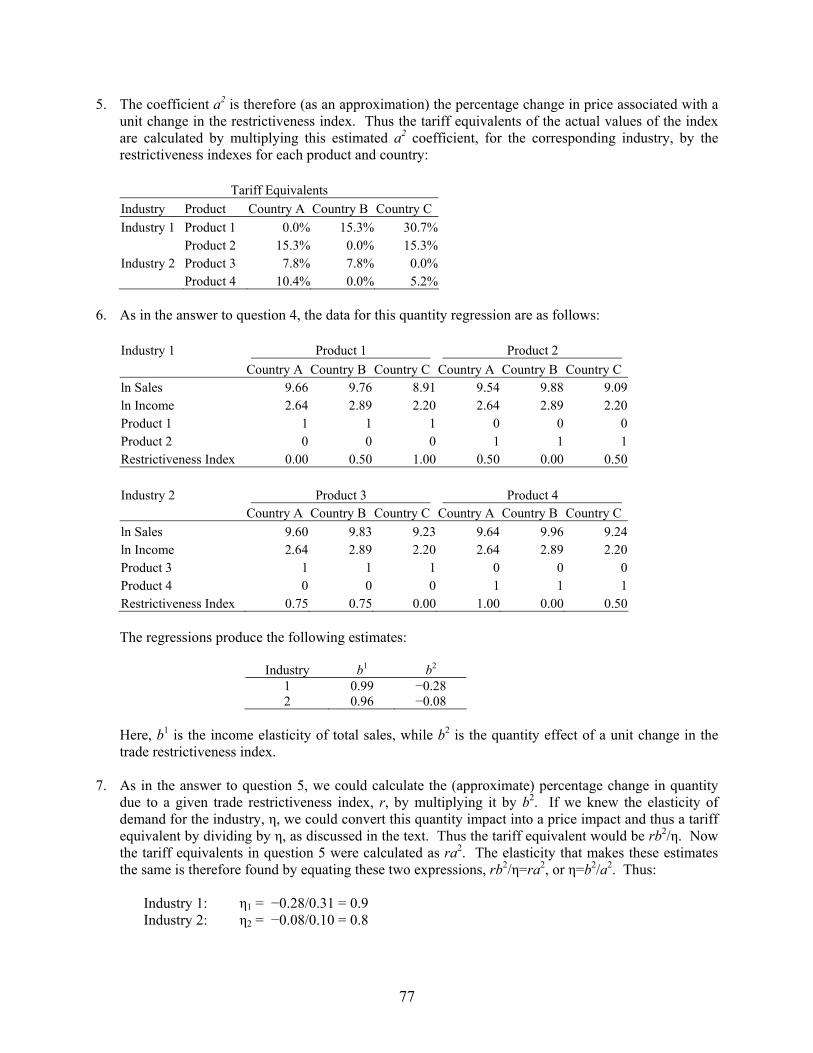
77

5. The coefficient a2 is therefore (as an approximation) the percentage change in price associated with a unit change in the restrictiveness index. Thus the tariff equivalents of the actual values of the index are calculated by multiplying this estimated a2 coefficient, for the corresponding industry, by the restrictiveness indexes for each product and country:

Tariff Equivalents

Industry Product Country A Country B Country C Industry 1 Product 1 0.0% 15.3% 30.7% Product 2 15.3% 0.0% 15.3%Industry 2 Product 3 7.8% 7.8% 0.0% Product 4 10.4% 0.0% 5.2%

6. As in the answer to question 4, the data for this quantity regression are as follows:

Industry 1 Product 1 Product 2 Country A Country B Country C Country A Country B Country C ln Sales 9.66 9.76 8.91 9.54 9.88 9.09 ln Income 2.64 2.89 2.20 2.64 2.89 2.20 Product 1 1 1 1 0 0 0 Product 2 0 0 0 1 1 1 Restrictiveness Index 0.00 0.50 1.00 0.50 0.00 0.50 Industry 2 Product 3 Product 4 Country A Country B Country C Country A Country B Country C ln Sales 9.60 9.83 9.23 9.64 9.96 9.24 ln Income 2.64 2.89 2.20 2.64 2.89 2.20 Product 3 1 1 1 0 0 0 Product 4 0 0 0 1 1 1 Restrictiveness Index 0.75 0.75 0.00 1.00 0.00 0.50

The regressions produce the following estimates:

Industry b1 b2

1 0.99 −0.28 2 0.96 −0.08

Here, b1 is the income elasticity of total sales, while b2 is the quantity effect of a unit change in the trade restrictiveness index.

7. As in the answer to question 5, we could calculate the (approximate) percentage change in quantity

due to a given trade restrictiveness index, r, by multiplying it by b2. If we knew the elasticity of demand for the industry, η, we could convert this quantity impact into a price impact and thus a tariff equivalent by dividing by η, as discussed in the text. Thus the tariff equivalent would be rb2/η. Now the tariff equivalents in question 5 were calculated as ra2. The elasticity that makes these estimates the same is therefore found by equating these two expressions, rb2/η=ra2, or η=b2/a2. Thus:

Industry 1: η1 = −0.28/0.31 = 0.9 Industry 2: η2 = −0.08/0.10 = 0.8