EmoPhoto: Identification of Emotions in Photos

Soraia Vanessa Meneses Alarcao Castelo

Thesis to obtain the Master of Science Degree in

Information Systems and Computer Engineering

Supervisor: Prof. Manuel Joao Caneira Monteiro da Fonseca

Examination Committee

Chairperson: Prof. Jose Carlos Martins DelgadoSupervisor: Prof. Manuel Joao Caneira Monteiro da Fonseca

Member of the Committee: Prof. Daniel Jorge Viegas Goncalves

October 2014

ii

Abstract

Nowadays, with the development in digital photography and the increasing easiness of acquiring cam-eras, taking pictures is a common task. Thus, the number of images in private collections of each personor in the Internet is becoming bigger.

Every time we use our collection of images, for example, to search for an image of a specific event,the images we receive will always be the same. However, our emotional state is not always the same:sometimes we are happy, and other times sad. Depending of the emotions perceived from the image,we are more receptive to some images than others. In the worst case, we will feel worse, which, giventhe importance of the emotions in our daily life, will lead to a significantly negative performance duringcognitive tasks such as attention or problem-solving.

Although it seems interesting to take advantage of the emotions that an image transmits, currentlythere is no way of knowing which emotions are associated with a given image. In order to identify theemotional content present in an image, as well as the category of those emotions (Negative, Positiveor Neutral), we describe in this document two approaches: one using Valence and Arousal information,and the other one using the content of the image.

The two developed recognizers achieved recognition rates of 89.20% and 68.68%, for the categoriesof emotions, and 80.13% for the emotions. Finally, we also describe a new dataset of images annotatedwith emotions, obtained from sessions with users.

Keywords: emotion recognition, emotions in images, fuzzy logic, content-based image retrieval, emotion-based image retrieval

iii

Resumo

Actualmente, com os desenvolvimentos na area da fotografia digital e a crescente facilidade de aquisicaode camaras fotograficas, tirar fotos tornou-se uma tarefa comum. Consequentemente, o numero de im-agens nas coleccoes particulares de cada pessoa, bem como das imagens disponıveis na Internet,aumentou.

Sempre que procuramos uma imagem de um determinado evento na nossa coleccao particular, asimagens apresentadas serao sempre as mesmas. No entanto, o nosso estado emocional nao per-manece igual: por vezes estamos felizes, e outras vezes tristes. Dependendo das emocoes percep-cionadas a partir de uma imagem, estamos mais receptivos a algumas imagens do que outras. Nopior caso, vamos sentir-nos pior, o que, dada a importancia das emocoes no nosso quotidiano, poderaconduzir a uma deterioracao no desempenho de tarefas a nıvel cognitivo, como atencao ou resolucaode problemas.

Embora pareca interessante aproveitar as emocoes transmitidas pelas imagens, actualmente naoexiste nenhuma forma de saber quais as emocoes que estao associadas a uma determinada imagem.A fim de identificar os conteudos emocionais presentes numa imagem, assim como a categoria dessesconteudos (negativa, positiva ou neutra), descrevemos neste documento duas abordagens: uma recor-rendo aos nıveis de Valencia e Excitacao da imagem, e uma outra utilizando o conteudo da mesma.

Os dois reconhecedores desenvolvidos alcancaram taxas de reconhecimento de 89.20% e 68.68%,para as categorias de emocoes, e 80.13% para as emocoes. Por fim, criamos um novo conjunto dedados de imagens anotadas com emocoes, obtidas a partir de sessoes com utilizadores.

Palavras-chave: reconhecimento de emocoes, emocoes em imagens, logica difusa, recuperacao deimagens baseada em conteudo, recuperacao de imagens baseada em emocoes

iv

Acknowledgments

I would like to thank my supervisor, Prof. Manuel Joao da Fonseca, not only for being an inspirationin the fields of Human-Computer Interaction and Multimedia Information Retrieval, but also for being asupportive and committed supervisor, who has always believed in my work, provided valuable feedbackand motivated me all the way through this journey. To Prof. Rui Santos Cruz, thank you for also encour-aging me to go even further in my academic choices and for being always available to sort out any issuethat I came across.

To my family, in general, thank you for forgiving my “absence” these past years due to my academiclife. To my brother Pedro Castelo, my sister Alexandra Castelo, and my sister-in-law Laura Pereira,thank you for all your support and care, and for making sure that I would withstand these past years. Tomy mother Carmo Meneses Alarcao, thank you for always believing in my success, and for being withgrandma when I was not able to. To Jorge Cabrita, thank you for being the “father” that I never had.To my second “mommy” Luısa Bravo da Mata, for encouraging me and always cheering me on eachdecision I took, thank you! My deepest, fondest and heartfelt thank you goes to my grandma AlcindaMeneses Alarcao, for all the sacrifices she made throughout her life in order to get me where I am now.Without her, I would not be who I am, and would not have gotten this far as I did.

In the last couple of years, I was fortunate to find true and amazing friends. Every time I washappy they were there to smile and celebrate with me. However, all the times I needed their support,they were also there: listening, helping, and most of the time, telling “our” silly jokes to cheer me up!Therefore, each one of you is the family that I chose: Ana Sousa, Andreia Ferrao, Bernardo Santos,Joana Condeco, Joao Murtinheira, Ines Bexiga, Ines Castelo, Ines Fernandes, Margarida Alberto, MariaJoao Aires, Miguel Coelho, Ricardo Carvalho, Rui Fabiano, and last, but not least, my “sister” VaniaMendonca.

A special thank you to my favorite “grammar-police” staff: Bernardo, Joao, Miguel, and Vania, foryour patience and availability to proof countless times for each part of this work. Thanks to all of you,this final version became much more complete and typo-free. I appreciate everything that you havetaught me, my English skills have improved so much! Catarina Moreira, Joao Vieira, and Joao SimoesPedro, thank you for your precious assistance with your knowledge of Machine Learning and Statistics.

Thank you to all the amazing people that I had the pleasure to work with these past years, whetherin class projects or other academic projects (especially NEIIST): David Duarte, David Silva, Fabio Alves,Luis Carvalho, Mauro Brito, Ricardo Laranjeiro, Rita Tome, among many others.

I would also like to thank to everyone who accepted to participate in the user sessions I performed inthe context of this thesis.

To each and every one of you - Thank you.

v

vi

To my grandma Alcinda

vii

viii

Contents

Abstract iii

Resumo iv

Acknowledgments v

List of Figures xii

List of Tables xiv

List of Acronyms xvii

1 Introduction 11.1 Motivation . . . . . . . . . . . . . . . . . . . . . . . . . . . . . . . . . . . . . . . . . . . . . 1

1.2 Goals . . . . . . . . . . . . . . . . . . . . . . . . . . . . . . . . . . . . . . . . . . . . . . . 2

1.3 Solution . . . . . . . . . . . . . . . . . . . . . . . . . . . . . . . . . . . . . . . . . . . . . . 2

1.4 Contributions and Results . . . . . . . . . . . . . . . . . . . . . . . . . . . . . . . . . . . . 3

1.5 Document Outline . . . . . . . . . . . . . . . . . . . . . . . . . . . . . . . . . . . . . . . . 3

2 Context and Related Work 52.1 Emotions . . . . . . . . . . . . . . . . . . . . . . . . . . . . . . . . . . . . . . . . . . . . . 5

2.2 Emotions in Images . . . . . . . . . . . . . . . . . . . . . . . . . . . . . . . . . . . . . . . 8

2.2.1 Content-Based Image Retrieval . . . . . . . . . . . . . . . . . . . . . . . . . . . . . 8

2.2.2 Facial-Expression Recognition . . . . . . . . . . . . . . . . . . . . . . . . . . . . . 10

2.2.3 Relationship between features and emotional content of an image . . . . . . . . . 13

2.3 Applications . . . . . . . . . . . . . . . . . . . . . . . . . . . . . . . . . . . . . . . . . . . . 16

2.3.1 Emotion-Based Image Retrieval . . . . . . . . . . . . . . . . . . . . . . . . . . . . 16

2.3.2 Recommendation Systems . . . . . . . . . . . . . . . . . . . . . . . . . . . . . . . 19

2.4 Datasets . . . . . . . . . . . . . . . . . . . . . . . . . . . . . . . . . . . . . . . . . . . . . . 20

2.5 Summary . . . . . . . . . . . . . . . . . . . . . . . . . . . . . . . . . . . . . . . . . . . . . 22

3 Fuzzy Logic Emotion Recognizer 233.1 The Recognizer . . . . . . . . . . . . . . . . . . . . . . . . . . . . . . . . . . . . . . . . . . 23

3.2 Experimental Results . . . . . . . . . . . . . . . . . . . . . . . . . . . . . . . . . . . . . . 35

3.3 Discussion . . . . . . . . . . . . . . . . . . . . . . . . . . . . . . . . . . . . . . . . . . . . 36

3.4 Summary . . . . . . . . . . . . . . . . . . . . . . . . . . . . . . . . . . . . . . . . . . . . . 37

ix

4 Content-Based Emotion Recognizer 394.1 List of features used . . . . . . . . . . . . . . . . . . . . . . . . . . . . . . . . . . . . . . . 404.2 Classifier . . . . . . . . . . . . . . . . . . . . . . . . . . . . . . . . . . . . . . . . . . . . . 41

4.2.1 One feature type combinations . . . . . . . . . . . . . . . . . . . . . . . . . . . . . 424.2.2 Two feature type combinations . . . . . . . . . . . . . . . . . . . . . . . . . . . . . 474.2.3 Three feature type combinations . . . . . . . . . . . . . . . . . . . . . . . . . . . . 484.2.4 Four feature type combinations . . . . . . . . . . . . . . . . . . . . . . . . . . . . . 484.2.5 Overall best features combinations . . . . . . . . . . . . . . . . . . . . . . . . . . . 48

4.3 Discussion . . . . . . . . . . . . . . . . . . . . . . . . . . . . . . . . . . . . . . . . . . . . 494.4 Summary . . . . . . . . . . . . . . . . . . . . . . . . . . . . . . . . . . . . . . . . . . . . . 50

5 Dataset 515.1 Image Selection . . . . . . . . . . . . . . . . . . . . . . . . . . . . . . . . . . . . . . . . . 515.2 Description of the Experience . . . . . . . . . . . . . . . . . . . . . . . . . . . . . . . . . . 515.3 Pilot Tests . . . . . . . . . . . . . . . . . . . . . . . . . . . . . . . . . . . . . . . . . . . . . 535.4 Results . . . . . . . . . . . . . . . . . . . . . . . . . . . . . . . . . . . . . . . . . . . . . . 535.5 Discussion . . . . . . . . . . . . . . . . . . . . . . . . . . . . . . . . . . . . . . . . . . . . 555.6 Summary . . . . . . . . . . . . . . . . . . . . . . . . . . . . . . . . . . . . . . . . . . . . . 57

6 Evaluation 596.1 Results . . . . . . . . . . . . . . . . . . . . . . . . . . . . . . . . . . . . . . . . . . . . . . 59

6.1.1 Fuzzy Logic Emotion Recognizer . . . . . . . . . . . . . . . . . . . . . . . . . . . . 596.1.2 Content-Based Emotion Recognizer . . . . . . . . . . . . . . . . . . . . . . . . . . 60

6.2 Discussion . . . . . . . . . . . . . . . . . . . . . . . . . . . . . . . . . . . . . . . . . . . . 616.3 Summary . . . . . . . . . . . . . . . . . . . . . . . . . . . . . . . . . . . . . . . . . . . . . 61

7 Conclusions and Future Work 637.1 Summary of the Dissertation . . . . . . . . . . . . . . . . . . . . . . . . . . . . . . . . . . 637.2 Final Conclusions and Contributions . . . . . . . . . . . . . . . . . . . . . . . . . . . . . . 657.3 Future Work . . . . . . . . . . . . . . . . . . . . . . . . . . . . . . . . . . . . . . . . . . . . 66

Bibliography 67

Appendix A 73

Appendix B 89

x

List of Figures

2.1 Universal basic emotions . . . . . . . . . . . . . . . . . . . . . . . . . . . . . . . . . . . . 62.2 Circumplex model of affect, which maps the universal emotions in the Valence-Arousal

plane. . . . . . . . . . . . . . . . . . . . . . . . . . . . . . . . . . . . . . . . . . . . . . . . 72.3 Wheel of Emotions . . . . . . . . . . . . . . . . . . . . . . . . . . . . . . . . . . . . . . . . 14

3.1 Circumplex Model of Affect with basic emotions. Adapted from [75] . . . . . . . . . . . . . 243.2 Distribution of the images in terms of Valence and Arousal . . . . . . . . . . . . . . . . . . 253.3 Polar Coordinate System for the distribution of the images . . . . . . . . . . . . . . . . . . 253.4 Sigmoidal membership function . . . . . . . . . . . . . . . . . . . . . . . . . . . . . . . . . 263.5 Trapezoidal membership function . . . . . . . . . . . . . . . . . . . . . . . . . . . . . . . . 263.6 2-D Membership Function . . . . . . . . . . . . . . . . . . . . . . . . . . . . . . . . . . . . 273.7 Membership Functions for Negative category . . . . . . . . . . . . . . . . . . . . . . . . . 283.8 2-D Membership Function . . . . . . . . . . . . . . . . . . . . . . . . . . . . . . . . . . . . 283.9 Membership Functions for Neutral category . . . . . . . . . . . . . . . . . . . . . . . . . . 283.10 2-D Membership Function . . . . . . . . . . . . . . . . . . . . . . . . . . . . . . . . . . . . 293.11 Membership Functions for Positive category . . . . . . . . . . . . . . . . . . . . . . . . . . 293.12 Membership Functions for Anger, Disgust and Sadness . . . . . . . . . . . . . . . . . . . 303.13 Membership Functions for Disgust . . . . . . . . . . . . . . . . . . . . . . . . . . . . . . . 303.14 Membership Functions for Disgust and Fear . . . . . . . . . . . . . . . . . . . . . . . . . . 313.15 Membership Functions for Disgust and Sadness . . . . . . . . . . . . . . . . . . . . . . . 323.16 Membership Functions for Fear . . . . . . . . . . . . . . . . . . . . . . . . . . . . . . . . . 323.17 Membership Functions for Happiness . . . . . . . . . . . . . . . . . . . . . . . . . . . . . 333.18 Membership Functions for Sadness . . . . . . . . . . . . . . . . . . . . . . . . . . . . . . 343.19 Membership Functions of Angle for all classes of emotions . . . . . . . . . . . . . . . . . 343.20 Membership Functions of Radius for all classes of emotions . . . . . . . . . . . . . . . . . 35

4.1 Average recognition considering all features . . . . . . . . . . . . . . . . . . . . . . . . . . 424.2 Results for Color - one feature . . . . . . . . . . . . . . . . . . . . . . . . . . . . . . . . . 434.3 Results for Color - two features . . . . . . . . . . . . . . . . . . . . . . . . . . . . . . . . . 444.4 Results for Color - three features . . . . . . . . . . . . . . . . . . . . . . . . . . . . . . . . 444.5 Time to build models . . . . . . . . . . . . . . . . . . . . . . . . . . . . . . . . . . . . . . . 46

5.1 EmoPhoto Questionnaire . . . . . . . . . . . . . . . . . . . . . . . . . . . . . . . . . . . . 525.2 Emotional state of the users in the beginning of the test . . . . . . . . . . . . . . . . . . . 535.3 Classification of the Negative images of our dataset (from users) . . . . . . . . . . . . . . 565.4 Classification of the Neutral and Positive images of our dataset (from users) . . . . . . . . 56

6.1 Classification of the Negative and Positive images of our dataset (from users) . . . . . . . 61

xi

B1 EmoPhoto Questionnaire . . . . . . . . . . . . . . . . . . . . . . . . . . . . . . . . . . . . 90B2 1. Age . . . . . . . . . . . . . . . . . . . . . . . . . . . . . . . . . . . . . . . . . . . . . . . 91B3 2. Gender . . . . . . . . . . . . . . . . . . . . . . . . . . . . . . . . . . . . . . . . . . . . . 91B4 3. Education Level . . . . . . . . . . . . . . . . . . . . . . . . . . . . . . . . . . . . . . . . 92B5 4. Have you ever participated in a study using any Brain-Computer Interface Device? . . . 92B6 7. How do you feel? . . . . . . . . . . . . . . . . . . . . . . . . . . . . . . . . . . . . . . . 93B7 8. Please classify your emotional state regarding the following cases: Anger, Disgust,

Fear, Happiness, Neutral, Sadness and Surprise . . . . . . . . . . . . . . . . . . . . . . . 93

xii

List of Tables

2.1 Comparision between International Affective Picture System (IAPS), Geneva AffectivePicturE Database (GAPED) and Mikels datasets . . . . . . . . . . . . . . . . . . . . . . . 21

3.1 Confusion Matrix for the classes of emotions in the IAPS dataset . . . . . . . . . . . . . . 363.2 Confusion Matrix for the categories in the Mikels dataset . . . . . . . . . . . . . . . . . . . 363.3 Confusion Matrix for the categories in the GAPED dataset . . . . . . . . . . . . . . . . . . 36

4.1 List of best features for each category type . . . . . . . . . . . . . . . . . . . . . . . . . . 474.2 Overall best features . . . . . . . . . . . . . . . . . . . . . . . . . . . . . . . . . . . . . . . 49

5.1 Confusion Matrix for the categories between Mikels and our dataset . . . . . . . . . . . . 555.2 Confusion Matrix for the categories between GAPED and our dataset . . . . . . . . . . . 56

6.1 Confusion Matrix for the categories using our dataset . . . . . . . . . . . . . . . . . . . . 596.2 Confusion Matrix for the categories using our dataset . . . . . . . . . . . . . . . . . . . . 60

A1 Simple and Meta classifiers results for each feature . . . . . . . . . . . . . . . . . . . . . . 73A2 Vote classifiers results for each feature . . . . . . . . . . . . . . . . . . . . . . . . . . . . . 73A3 Results for Color using one feature . . . . . . . . . . . . . . . . . . . . . . . . . . . . . . . 74A4 Results for combination of two Color features . . . . . . . . . . . . . . . . . . . . . . . . . 74A5 Results for combination of three Color features . . . . . . . . . . . . . . . . . . . . . . . . 75A6 Results for combination of four Color features . . . . . . . . . . . . . . . . . . . . . . . . . 76A7 Results for combination of five Color features . . . . . . . . . . . . . . . . . . . . . . . . . 76A8 Results for combination of six Color features . . . . . . . . . . . . . . . . . . . . . . . . . 76A9 Results for combination of seven Color features . . . . . . . . . . . . . . . . . . . . . . . . 77A10 Results for combination of all Color features . . . . . . . . . . . . . . . . . . . . . . . . . . 77A11 List of candidate features for Color . . . . . . . . . . . . . . . . . . . . . . . . . . . . . . . 78A12 Results for Composition feature . . . . . . . . . . . . . . . . . . . . . . . . . . . . . . . . . 78A13 Results for combination of Shape features . . . . . . . . . . . . . . . . . . . . . . . . . . . 78A14 Results for combination of Texture features . . . . . . . . . . . . . . . . . . . . . . . . . . 78A15 Results for combination of Joint features . . . . . . . . . . . . . . . . . . . . . . . . . . . . 79A16 Results for combination of Color and Composition features . . . . . . . . . . . . . . . . . 79A17 Results for combination of Color and Shape features . . . . . . . . . . . . . . . . . . . . . 79A18 Results for combination of Color and Texture features . . . . . . . . . . . . . . . . . . . . 79A19 Results for combination of Color and Joint features . . . . . . . . . . . . . . . . . . . . . . 80A20 Results for combination of Composition and Shape features . . . . . . . . . . . . . . . . . 80A21 Results for combination of Composition and Texture features . . . . . . . . . . . . . . . . 80A22 Results for combination of Composition and Joint features . . . . . . . . . . . . . . . . . . 80

xiii

A23 Results for combination of Shape and Texture features . . . . . . . . . . . . . . . . . . . . 80A24 Results for combination of Shape and Joint features . . . . . . . . . . . . . . . . . . . . . 81A25 Results for combination of Texture and Joint features . . . . . . . . . . . . . . . . . . . . . 81A26 Results for combination of Color, Composition and Shape features . . . . . . . . . . . . . 81A27 Results for combination of Color, Composition and Texture features . . . . . . . . . . . . . 81A28 Results for combination of Color, Composition and Joint features . . . . . . . . . . . . . . 82A29 Results for combination of Color, Shape and Texture features . . . . . . . . . . . . . . . . 82A30 Results for combination of Color, Shape and Joint features . . . . . . . . . . . . . . . . . 82A31 Results for combination of Color, Texture and Joint features . . . . . . . . . . . . . . . . . 83A32 Results for combination of Color, Composition, Texture and Shape features . . . . . . . . 83A33 Results for combination of Color, Composition, Texture and Joint features . . . . . . . . . 84A34 Results for combination of Color, Texture, Joint and Shape features . . . . . . . . . . . . . 84A35 Results for combination of Color, Texture, Joint and Composition features . . . . . . . . . 84A36 Confusion Matrices for each combination . . . . . . . . . . . . . . . . . . . . . . . . . . . 85A37 Confusion Matrices for each combination using GAPED dataset with Negative and Posi-

tive categories . . . . . . . . . . . . . . . . . . . . . . . . . . . . . . . . . . . . . . . . . . 86A38 Confusion Matrices for each combination using GAPED dataset with Negative, Neutral

and Positive categories . . . . . . . . . . . . . . . . . . . . . . . . . . . . . . . . . . . . . 87A39 Confusion Matrices for each combination using Mikels and GAPED dataset . . . . . . . . 88

xiv

List of Acronyms

AAM Active Appearance Models

ACC AutoColorCorrelogram

ADF Anger, Disgust and Fear

ADS Anger, Disgust and Sadness

AF Anger and Fear

AM Affective Metadata

ANN Artificial Neural Network

AS Anger and Sadness

AU Action Unit

Bag Bagging

BCI Brain-Computer Interfaces

CBIR Content-based Image Retrieval

CBER Content-based Emotion Recognizer

CBR Content-based Recommender

CCV Color Coherence Vectors

CEDD Color and Edge Directivity Descriptor

CF Collaborative-Filtering

CH Color Histogram

CM Color Moments

CMA Circumplex Model of Affect

D Disgust

DF Disgust and Fear

DOM Degree of Membership

DOF Depth of Field

DS Disgust and Sadness

xv

EBIR Emotion-based Image Retrieval

EEG Electroencephalography

EH Edge Histogram

F Fear

FCP Facial Characteristic Point

FCTH Fuzzy Color and Texture Histogram

FE Feature Extraction

FLER Fuzzy Logic Emotion Recognizer

FER Facial Expression Recognition

FCTH Fuzzy Color and Texture Histogram

FS Fear and Sadness

G Gabor

GAPED Geneva Affective PicturE Database

GLCM Gray-Level Co-occurence Matrix

GM Generic Metadata

GMM Gaussian Mixture Models

GPS Global Positioning System

Ha Happiness

H Haralick

HSV Hue, Saturation and Value

IAPS International Affective Picture System

IBk K-nearest neighbours

IGA Interactive Genetic Algorithm

J48 C4.5 Decision Tree (algorithm from Weka)

JCD Joint Composite Descriptor

KDEF Karolinska Directed Emotional Faces

LB LogitBoost

Log Logistic

MHCPH Modified Human Colour Perception Histogram

MIP Mood-Induction Procedures

MLP Multi-Layer Percepton

xvi

NB Naive Bayes

NDC Number of Different Colors

OH Opponent Histogram

PCA Principal Component Analysis

PFCH Perceptual Fuzzy Color Histogram

PFCHS Perceptual Fuzzy Color Histogram with 3x3 Segmentation

POFA Pictures of Facial Affect

PVR Personal Video Recorders

RCS Reference Color Similarity

RecSys Recommendation Systems

RF Random Forest

RSS RandomSubSpace

RT Rule of Thirds

S Sadness

SAM Self-Assessment Manikin

SM Similarity Measurement

SMO John Platt’s sequential minimal optimization algorithm for training a support vector classifier

SPCA Shift-invariant Principal Component Analysis

Su Surprise

SVM Support Vector Machine

T Tamura

V1 Vote 1

V2 Vote 2

V3 Vote 3

V4 Vote 4

V5 Vote 5

V6 Vote 6

VAD Valence, Arousal and Dominance

VOD Video-On-Demand systems

xvii

xviii

1Introduction

In this chapter we present our motivation, the goals we intend to achieve, as well as the solution devel-oped to identify emotions, in particular the Fuzzy Logic Emotion Recognizer (FLER) and the Content-based Emotion Recognizer (CBER). We also enumerate the main contributions and results of our work,as well as the document outline.

1.1 Motivation

Images are an increasingly important class of data, especially as computers become more usable,with greater memory and communication capacities [42]. Nowadays, with the development in digitalphotography and the increasing easiness of acquiring cameras and smartphones, taking pictures (andstoring them) is a common task. Thus, the number of images in private collections of each person isbecoming bigger. In the case of the images available in the internet, it is not big, it is huge.

With this massive growth in the amount of visual information available, the need to store and retrieveimages in an efficient manner arises, leading to an increase of the importance of Content-based ImageRetrieval (CBIR) systems [78]. However, these systems do not take into account high level features likehuman emotions associated with the images or the emotional state of the users. To overcome this, anew technique, Emotion-based Image Retrieval (EBIR) was proposed in order to extend CBIR systemsthrough the use of human emotions besides common features [81, 87]. Currently, emotion or moodinformation are already used as search terms within multimedia databases, retrieval systems or evenmultimedia players.

We can interact with and explore image collections in many ways. One possibility is through theircontent, such as Colors, Shapes, Texture and Lines, or through associated information such as tags,data or Global Positioning System (GPS) information. Every time we search for something, for examplefor images from a specific day or event, the order in which the images are presented can be different butthe images will always be the same. However, our emotional state is not always the same: sometimeswe are happy, and other times sad or depressed. Therefore we are more receptive to some images thanothers, depending of the emotions perceived from the image.

In the image domain, emotions describe the personal affectedness based on spontaneous perception

1

[19], and can be achieved, for example, through the colors or facial expressions of people present in theimage. In the worst case, these results will make us feel even worse, which, given the importance of theemotions in our daily life, will lead to a significantly negative performance during cognitive tasks such asattention, creativity, memory, decision-making, judgment, learning or problem-solving.

Although it seems interesting to take advantage of the emotions that an image transmits, for example,by using them to explore a collection of images, currently there is no way of knowing which emotionsare associated with a given image. In order to identify the emotional content present in an image, i.e.,the emotions that would be triggered when viewing the image, as well as the corresponding category ofthose emotions (Negative, Positive or Neutral), we will follow two approaches: one using Valence andArousal information, and the other one using the content of the image.

1.2 Goals

This work aims to be able to identify the emotional content present in an image, regarding the corre-sponding category of emotions, i.e., if an image transmits Negative, Positive or Neutral feelings to theviewer. We also want to be able to give an insight about what emotions would be triggered when viewingan image.

To that end, we plan to take advantage of the Valence and Arousal values associated to somedatasets of images, and in the case where there are no information about V-A, we plan to use thecontent of the images to derive the emotion or category of emotion that it conveys to the viewer.

To achieve this, we need to focus on three different sub-goals: i) develop an emotion recognizerbased on the Valence and Arousal information associated to images; ii) develop an emotion recognizerbased on the visual content of the images, such as Colors, Shape or Texture; iii) finally, we want to collectinformation, using people, about the dominant emotions transmitted by a set of images, by performingan experiment with people.

1.3 Solution

The solution developed, in the context of this work, consists in two recognizers that are able to identifythe emotional content of an image using different inputs, and producing different levels of output.

The first recognizer, Fuzzy Logic Emotion Recognizer (FLER), uses the normalized values of Valenceand Arousal of an image to automatically classify the classes of emotions: Anger, Disgust and Sadness(ADS), Disgust (D), Disgust and Fear (DF), Disgust and Sadness (DS), Fear (F), Happiness (Ha), andSadness (S) and categories: Positive, Neutral and Negative, conveyed by an image. To describe eachclass of emotions, as well as the categories, we used a Fuzzy Logic approach, in which each set ischaracterized by a membership function that assigns to each object a Degree of Membership layingbetween zero and one [90]. In the case of emotions, we used the Product of Sigmoidal membershipfunction for the Angle that correlates Valence and Arousal values, and Trapezoidal membership functionfor the Radius, that will help to reduce emotion confusion between images with similar Angles. Regardingthe categories we used the Trapezoidal membership function, both for the Angle and the Radius. Finally,for each class of emotions and category, we used a two-dimensional membership function that is theresult of the composition of the two one-dimensional membership functions mentioned above.

The second recognizer, Content-based Emotion Recognizer (CBER), uses visual content informationof the image to automatically classify if an image is Negative or Positive. To select the best descriptorsto use, we performed a large number of tests using different combinations of Color, Texture, Shape,Composition and Joint descriptors/features. We started by analyzing a set of classifiers, in order tounderstand which one best learns the relationship between features and the given category of emotion.

2

After that, and based on the relationships found, we proposed six different combinations of classifiersusing the Vote classifier as a base. For each of the proposed combinations of classifiers, we testedseveral feature combinations. In the end, the best solution is composed by a Vote classifier, containingJohn Platt’s sequential minimal optimization algorithm for training a support vector classifier (SMO),Naive Bayes (NB), LogitBoost (LB), Random Forest (RF), and RandomSubSpace (RSS), and a combi-nation of features, which include the Color Histogram (CH), Color Moments (CM), Number of DifferentColors (NDC), and Reference Color Similarity (RCS).

1.4 Contributions and Results

With the completion of this thesis, we achieved three main contributions:

• A Fuzzy recognizer with a classification rate of 100% in the case of categories and 91.56% in thecase of emotions, for Mikels dataset [66]; with the Geneva Affective PicturE Database (GAPED)we achieved an average classification rate of 95.59% for the categories. Using our dataset, weachieved a success rate of 68.70% for emotions. In the case of categories, we achieved 100% forNegative category, 85% for the Positive and 28% for the Neutral.

• A recognizer based on the content of the images, that has a recognition rate of 87.18% for theNegative category, and 57.69% for the Positive, using a dataset of images selected both fromInternational Affective Picture System (IAPS) and from GAPED datasets. Using our dataset, weachieved a recognition rate of 76.54% for the Negative category and 52.38% for the Positive.

• A new dataset of 169 images from IAPS, Mikels and GAPED annotated with the dominant cate-gories and emotions, according to what people felt while viewing each image.

1.5 Document Outline

In chapter 2, we describe the importance of emotions, as well as how they can be represented. Alongwith it, we detail the previous works in the recognition of emotions from images, how to identify theemotional state of a user, and some research areas where these two topics are combined: Emotion-based Image Retrieval (EBIR) and Recommendation Systems (RecSys). We also describe the rela-tionship between emotions and the different visual characteristics of an image. Finally, we present thedatasets that we used in our work: International Affective Picture System (IAPS), Geneva AffectivePicturE Database (GAPED) and Mikels.

In chapter 3, we describe the Fuzzy Logic Emotion Recognizer (FLER) and the corresponding exper-imental results achieved, while in chapter 4, both the Content-based Emotion Recognizer (CBER) andthe experimental results obtained are described. We also present an analysis of the different possiblecombinations between the different types of features used: Color, Texture, Composition, and Shape.

In chapter 5, we present a new dataset that is annotated with information collected through experi-ments with users. In chapter 6, we present the evaluation of FLER and CBER using our new annotateddataset.

Finally, a summary of the dissertation, the conclusions and future work are presented in chapter 7.

3

4

2Context and Related Work

Within this chapter we present a review and summary of the related works in the fields of emotions,the recognition of the emotions in images using Content-based Image Retrieval (CBIR) and Facial Ex-pression Recognition (FER), as well as the relationship between the emotions and the visual charac-teristics mentioned in CBIR, and finally Emotion-based Image Retrieval (EBIR) and RecommendationSystems (RecSys). Although this seems to be a lot of fields, some of them such as emotions, andRecSys are described here only to give some context, while CBIR, FER and EBIR are our main focus.We also present and describe the datasets used in our work.

2.1 Emotions

“An emotion is a complex psychological state that involves three distinct components: asubjective experience, a physiological response, and a behavioral or expressive response.”[35]

Emotions have been described as discrete and consistent responses to external or internal eventswith particular significance for the organism. They are brief in duration and correspond to a coordinatedset of responses, which may include verbal, behavioral, physiological and neural mechanisms. In af-fective neuroscience, the emotion can be differentiated from similar constructs like feelings, moods andaffects. Feelings can be viewed as a subjective representation of emotions. Moods are diffuse affectivestates that generally last for much longer durations than emotions and are also usually less intense thanemotions. Finally, affect is an encompassing term, used to describe the topics of emotion, feelings, andmoods together [23].

The role of emotion in human cognition is essential. Emotions also play a critical role in rationaldecision-making, perception, human interaction, and in human intelligence [69]. Emotions play an im-portant role in the daily life of human beings. The importance (and need) of automatic emotion recogni-tion has grown with the increasing role of human-computer interface applications. Nowadays, new formsof human-centric and human-driven interaction with digital media have the potential of revolutionizingentertainment, learning, and many other areas of life. Emotion recognition could be done from text,speech, facial expressions or gestures [54].

5

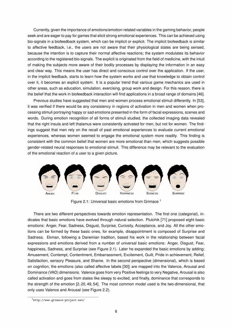
Currently, given the importance of emotions/emotion-related variables in the gaming behavior, peopleseek and are eager to pay for games that elicit strong emotional experiences. This can be achieved usingbio-signals in a biofeedback system, which can be implicit or explicit. The implicit biofeedback is similarto affective feedback, i.e., the users are not aware that their physiological states are being sensed,because the intention is to capture their normal affective reactions; the system modulates its behavioraccording to the registered bio-signals. The explicit is originated from the field of medicine, with the intuitof making the subjects more aware of their bodily processes by displaying the information in an easyand clear way. This means the user has direct and conscious control over the application. If the user,in the implicit feedback, starts to learn how the system works and use that knowledge to obtain controlover it, it becomes an explicit system. It is a popular trend that various game mechanics are used inother areas, such as education, simulation, exercising, group work and design. For this reason, there isthe belief that the work in biofeedback interaction will find applications in a broad range of domains [46].

Previous studies have suggested that men and women process emotional stimuli differently. In [53],it was verified if there would be any consistency in regions of activation in men and women when pro-cessing stimuli portraying happy or sad emotions presented in the form of facial expressions, scenes andwords. During emotion recognition of all forms of stimuli studied, the collected imaging data revealedthat the right insula and left thalamus were consistently activated for men, but not for women. The find-ings suggest that men rely on the recall of past emotional experiences to evaluate current emotionalexperiences, whereas women seemed to engage the emotional system more readily. This finding isconsistent with the common belief that women are more emotional than men, which suggests possiblegender-related neural responses to emotional stimuli. This difference may be relevant to the evaluationof the emotional reaction of a user to a given picture.

Figure 2.1: Universal basic emotions from Grimace 1

There are two different perspectives towards emotion representation. The first one (categorial), in-dicates that basic emotions have evolved through natural selection. Plutchik [71] proposed eight basicemotions: Anger, Fear, Sadness, Disgust, Surprise, Curiosity, Acceptance, and Joy. All the other emo-tions can be formed by these basic ones, for example, disappointment is composed of Surprise andSadness. Ekman, following a Darwinian tradition, based his work in the relationship between facialexpressions and emotions derived from a number of universal basic emotions: Anger, Disgust, Fear,happiness, Sadness, and Surprise (see Figure 2.1). Later he expanded the basic emotions by adding:Amusement, Contempt, Contentment, Embarrassment, Excitement, Guilt, Pride in achievement, Relief,Satisfaction, sensory Pleasure, and Shame. In the second perspective (dimensional), which is basedon cognition, the emotions (also called affective labels [30]) are mapped into the Valence, Arousal andDominance (VAD) dimensions. Valence goes from very Positive feelings to very Negative, Arousal is alsocalled activation and goes from states like sleepy to excited, and finally, dominance that corresponds tothe strength of the emotion [2, 20, 49, 54]. The most common model used is the two-dimensional, thatonly uses Valence and Arousal (see Figure 2.2).

1http://www.grimace-project.net/

6

Figure 2.2: Circumplex model of affect, which maps the universal emotions in the Valence-Arousal plane.

In [76], some correlations between basic emotions were described. One of the most important resultswas that when happiness rises, all other emotions decline, and the other one, that Fear correlatespositively with Sadness and with Anger. These correlations are well-known phenomena in the field ofpsychology.

Many studies in psychology involve manipulating Valence and/or Arousal via emotional stimuli. Thistechnique of inducing emotion in human participants is referred to as affective priming. Several methodshave been introduced for priming participants with Positive or Negative affect. Common methods includeimages, text (stories), videos, sounds, word-association tasks, and combinations thereof. Such methodsare commonly referred to as Mood-Induction Procedures (MIP). In general, Positive emotions tend tolead to better cognitive performance, and Negative emotions (with some exceptions) lead to decreasedperformance [32].

Affective computing is a rising topic within human-computer interaction that tries to satisfy other userneeds, besides the need of the user to be as productive as possible. As the user is an affective hu-man being, many needs are related to emotions and interaction [5]. Research has already been doneinto recognizing emotions from faces and voice. Humans can recognize emotions from these signalswith a 70-98% accuracy, and computers are already pretty successful especially at classifying facialexpressions (80-90%). With the rising interest for Brain-Computer Interfaces (BCI), user’s Electroen-cephalography (EEG) have been analyzed as well [5].

In [2], they use information about the affective/mental states of users to adapt interfaces or add func-tionalities. In [32], the authors describe a crowdsourced experiment in which affective priming is used toinfluence low-level visual judgment performance. They present results that suggest that affective primingsignificantly influences visual judgments, and that Positive priming increases performance. Additionally,individual personality differences can influence performance with visualizations. In addition to stablepersonality traits, research in psychology has found that temporary changes in affect (emotion) can alsosignificantly impact performance during cognitive tasks such as memory, attention, learning, judgment,creativity, decision-making, and problem-solving.

7

The category-based models can be used for tagging purposes, specially with a list of different adjec-tives for the same mood, which allows the generalization of the subjective perceptions of multiple usersand provides a dictionary for search and retrieval applications [19]. However, the dimensional model ispreferable in emotion recognition experiments because a dimensional model can locate discrete emo-tions in its space, even when no particular label can be used to define a certain feeling [54].

For our work, we will use the six universal basic emotions with the addition of a new emotion: theNeutral. To map the emotions into a two-dimensional model (since it is better for the purpose of ourwork), an adaptation of the circumplex model of affect introduced in [72] will be used (see Figure 2.2) [83].

2.2 Emotions in Images

In order to extract emotions from an image, we need to understand how their contents affect the wayemotions are perceived by users. For example, different Colors give us different feelings: bright Colorshelp to create a Positive and friendly mood whereas dark Colors create the opposite. In the other hand,the lines such as the diagonal ones indicate activity, and the horizontal ones express calmness.

In the human interaction, if we communicate with someone that appears to be sad, we tend tosympathize with that person and feel sad too. However, if the person is happy we tend to becomehappier. The same effect is observed in case we see sad or happy expressions in pictures, i.e., it willalso affect our emotional state.

2.2.1 Content-Based Image Retrieval

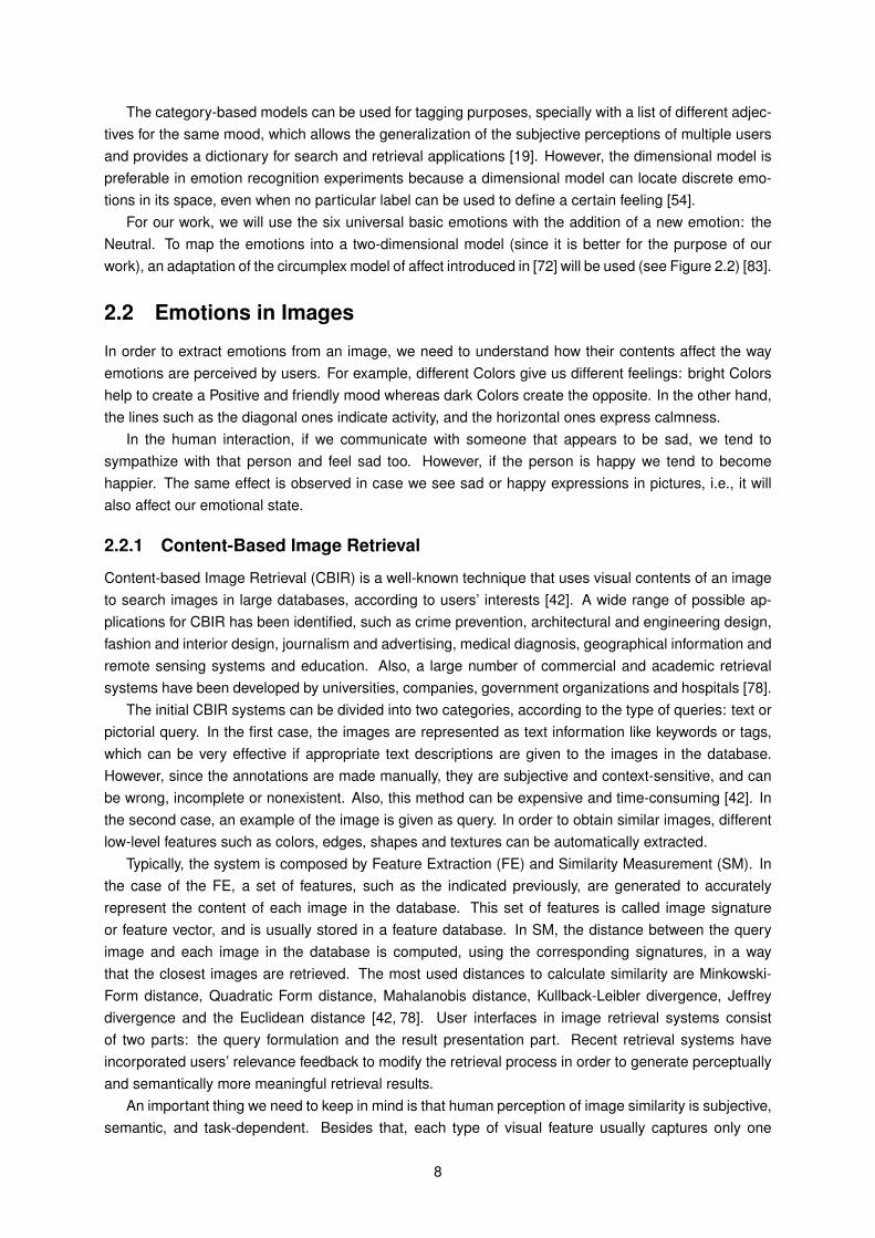
Content-based Image Retrieval (CBIR) is a well-known technique that uses visual contents of an imageto search images in large databases, according to users’ interests [42]. A wide range of possible ap-plications for CBIR has been identified, such as crime prevention, architectural and engineering design,fashion and interior design, journalism and advertising, medical diagnosis, geographical information andremote sensing systems and education. Also, a large number of commercial and academic retrievalsystems have been developed by universities, companies, government organizations and hospitals [78].

The initial CBIR systems can be divided into two categories, according to the type of queries: text orpictorial query. In the first case, the images are represented as text information like keywords or tags,which can be very effective if appropriate text descriptions are given to the images in the database.However, since the annotations are made manually, they are subjective and context-sensitive, and canbe wrong, incomplete or nonexistent. Also, this method can be expensive and time-consuming [42]. Inthe second case, an example of the image is given as query. In order to obtain similar images, differentlow-level features such as colors, edges, shapes and textures can be automatically extracted.

Typically, the system is composed by Feature Extraction (FE) and Similarity Measurement (SM). Inthe case of the FE, a set of features, such as the indicated previously, are generated to accuratelyrepresent the content of each image in the database. This set of features is called image signatureor feature vector, and is usually stored in a feature database. In SM, the distance between the queryimage and each image in the database is computed, using the corresponding signatures, in a waythat the closest images are retrieved. The most used distances to calculate similarity are Minkowski-Form distance, Quadratic Form distance, Mahalanobis distance, Kullback-Leibler divergence, Jeffreydivergence and the Euclidean distance [42, 78]. User interfaces in image retrieval systems consistof two parts: the query formulation and the result presentation part. Recent retrieval systems haveincorporated users’ relevance feedback to modify the retrieval process in order to generate perceptuallyand semantically more meaningful retrieval results.

An important thing we need to keep in mind is that human perception of image similarity is subjective,semantic, and task-dependent. Besides that, each type of visual feature usually captures only one

8

aspect of image property, and it is usually hard for the user to specify clearly how different aspects arecombined. However, there is no single “best” feature that gives accurate results in any general setting,which means that, usually, a combination of features is needed to provide adequate retrieval results [78].

Nowadays, researchers are merging fields such as computer vision, machine learning and imageprocessing, which provides an opportunity to find solutions of different issues such as semantic gap anddimensionality reduction [42]. Semantic gap shows the difference between high-level concepts suchas emotions, events, objects or activities as conveyed by an image and limited descriptive power oflow-level visual features.

After the CBIR technical/theoretical characteristics have been explained, it is important to explain thevisual features that this technique uses:

Color:This is the most extensively used visual content for image retrieval since it is the basic constituentof images. It is relatively robust to background complication and independent of orientation andimage size. In some works like [78], grayscale is also considered as a color. Usually, in thesesystems, Color histogram is the most used feature representation and gives us the descriptionof the colors present in an image as well as their quantities. It is obtained by quantizing imagecolor into discrete levels, then the number of times each discrete occur in the image is counted.They are insensitive to small perturbations in camera position and are computationally efficient tocompute.

When a database contains a large number of images, histogram comparison will saturate thediscrimination. To solve this problem, the joint histogram technique [27] was introduced, in whichit is incorporated additional information without affecting the robustness of Color histograms.

It is possible that two different images have the same Color histogram because a single Colorhistogram extracted from an image lacks spatial information of colors in the image. In [78], theauthors expose different possible solutions. In the first one, a CBIR takes account of the spatialinformation of the Colors by using multiple histograms. In the second one, the spatial featuresarea (zero-order) and position (first-order) moments are used for retrieval. Finally, in the last one,a different way of incorporating spatial information into the Color histogram, Color CoherenceVectors (CCV), was proposed. Using the Color correlogram, it is possible to characterize not onlythe color distributions of pixels, but also the spatial correlation of pairs of colors.

Modified Human Colour Perception Histogram (MHCPH) [77] is based on human visual perceptionof the Color. The gray weights and color are distributed to neighboring bins smoothly with respectto pixel information. The amount of weight that is distributed to the neighboring bins is estimatedusing NBS distance, which makes it possible to extract the background color information effectivelyalong with the foreground information.

Shape:It corresponds to an important criterion for matching objects based on their physical structure andprofile. Shape is a well-defined concept and there is considerable evidence that natural objects areprimarily recognized by their shape [78]. These features can represent the spacial information thatis not represented by Texture or Color, and contains all the geometrical information of an objectin the image. This information does not change even if the location or orientation of the objectchanges.

The simplest Shape features are the perimeter, area, eccentricity and symmetry [42], but, usually,two main types of Shape features are commonly used: global features and local features. Aspect

9

ratio, circularity and moment invariants are examples of global features and sets of consecutiveboundary segments corresponds to local features.

Shape representations can be divided into two classes: boundary-based and region-based. Inthe first case, only the outer boundary of the shape is used. The most common approaches arethe rectilinear shapes, polygonal approximation, finite element models, and Fourier-based shapedescriptors. In the second one, the entire Shape region is used to compute statistical moments.A good Shape representation feature for an object should be invariant to translation, rotation andscaling [78].

Texture:It is defined as all that it is left after Color and local Shape has been considered. It is used tolook for visual patterns, with properties of homogeneity that are not achieved by the presence of asingle color, in images and how they are spatially defined. Also, it contains information about thestructural arrangement of surfaces and their relationship to the surrounding environment. Texturesimilarity can be used to distinguishing between areas of images with similar Color such as skyand sea. Texture representation can be classified into three categories: statistical, structural andspectral.

In the statistical approach, the Texture is characterized using the statistical properties of the graylevels in the pixels of the image. Usually, there is a periodic occurrence of certain gray levels.Some of the methods used are co-occurrence matrix, Tamura features, Shift-invariant PrincipalComponent Analysis (SPCA), Wold decomposition and multi-resolution filtering techniques suchas Gabor and Wavelet transform. Both the Tamura features and Wold decomposition are designedaccording to physiological studies on the human perception of Texture and described in terms ofperceptual properties.

The structural methods describe the Texture as a composition of texels (texture elements) that arearranged regularly on a surface according to some specific arrangement rules. Some methods,such as morphological operator and adjacency graphs, describe the Texture by the identificationof structural primitives and their corresponding placement rules. If they are applied to regulartextures, they tend to be very effective [78].

In the spectral method, the Texture description is done by using a Fourier transform of an imageand then group the transformed data in a way that it gives some set of measurements.

These descriptions allowed us to understand how Color, Shape and Texture are characterized, aswell as how they usually appear in an image. It also allowed us to identify the visual descriptors and thedifferent approaches that are most commonly used to capture each of the visual features used in CBIRsystems.

2.2.2 Facial-Expression Recognition

The human face is one of the major ”objects” in our daily lives that is used to provide information aboutthe gender, attractiveness and age of a person, but also helps to identify the emotion that person isfeeling; this has an important role in human communication.

Underneath our skin, a large number of face muscles allow us to produce different configurations.These muscles can be summarized as Action Unit (AU) [21] and are used to define the facial expressionsof an emotion. Facial expressions are typically classified as Joy, Surprise, Anger, Sadness, Disgust andFear [15,21].

Recent research in cognitive science and neuroscience has shown that humans use mostly theShape for the perception and recognition of facial expressions of emotion. Furthermore, humans are

10

very good only at recognizing a few facial expressions of emotion. The most well recognized emotionsare Happiness and Surprise and the worst are Fear and Disgust. Learning why our visual system easilyrecognizes some expressions and not others should help the definition of the form and dimensions ofthe computational model of facial expressions of emotion [63].

To describe how humans perceive and classify facial expressions of an emotion, there are two typesof models: the continuous and categorical. In the first one, each facial expression of an emotion isdefined as a feature vector in a face space, given by some characteristics that are common to all theemotions. In the second one, there are C classifiers, each one associated to a specific emotion category.The continuous model explains how expressions of emotion can be seen at different intensities, whereasthe categorical explains, among other findings, why the images in a morphing sequence between twoemotions, like happiness and surprise, are perceived as either happy or surprise but not something inbetween. Also several psychophysical experiments suggest the perception of emotions by humans iscategorical [22].

There have been developed models of the perception and classification of the six facial expressionsof emotion, in which sample feature vectors or regions of the feature space are used to represent eachone of the emotion labels, but only one emotion can be detected from a single image, despite the fact thathumans can perceive more than one emotion in a single image, even if they have no prior experiencewith it.

Initially, researchers have created several feature and shape-based algorithms for recognition ofobjects and faces [40, 55, 61], in which geometric, Shape features and edges were extracted from animage and used to create a model of the face. Then, this model was fitted to the image, and in case ofa good fit, it is used to determine the class and position of the face.

In [63], an independent computational (face) space for a small number of emotion labels was pre-sented. In this approach, it is only needed to sample faces of those few facial expressions of emo-tion. This approach corresponds to a categorical model, however the authors define each of these facespaces as continue feature spaces. Essentially, the observed intensity in this continuous representationis used to define the weight of the contribution of each basic category toward the final classification,allowing the representation and recognition of a very large number of emotion categories without theneed to have a categorical space for each one or having to use many samples of each expression asin the continuous model. With this approach, a new model was introduced; it consists of C distinct con-tinuous spaces, in which multiple emotion categories can be recognized by linearly combining these C

face spaces. The most important aspect of this model is that it is possible to define new categories aslinear combinations of a small set of categories. The proposed model thus bridges the gap between thecategorical and continuous ones and resolves most of the debate facing each of the models.

The authors explained that the face spaces should include configural and shape features, becausethe configural features can be obtained from an appropriate representation of shape, however expres-sions such as Fear and Disgust seem to be mostly based on Shape features, making the recognitionprocess less accurate and more susceptible to image manipulation. Each one of the six categories ofemotion used is represented in a shape space given by classical statistical shape analysis. The faceand the shape of the major facial components are automatically detected, i.e., the brows, eyes, nose,mouth and jaw line. Then, the shape is sampled with d equally spaced landmark points and the meanof all the points is computed.

To provide invariance to translation and scale, the 2d-dimensional shape feature vector is given bythe x and y coordinates of the d shape landmarks subtracted by the mean and divided by its norm. In thecase of the 3D rotation invariance, it can be achieved with the inclusion of a kernel. The authors usedthe algorithm defined by [29] to obtain the dimensions of each emotion category, because it minimizesthe Bayes classification error.

11

Since two categories can be connected by a more general one, the authors use the already definedshape space to find the two most discriminant dimensions separating each of the six categories previ-ously listed. Then, in order to test the model, they trained a linear Support Vector Machine (SVM) andachieved the following results: Happiness is correctly classified 99% of the times, Surprise and Disgust95%, Sadness 90%, Fear 92% and Anger 94%. They also mentioned that adding new dimensions inthe feature space and using nonlinear classifiers makes it possible to achieve perfect classification.

In the last two decades, a new approach was studied: appearance-based, in which the faces arerepresented by their pixel-intensity maps or the response to some filters (e.g. Gabors). The mainadvantage of appearance-based model is that there is no need to: predefine a feature/shape modellike in the previous approaches, since the face model is given by the training images. Also, it providesgood results for near-frontal images of good quality, but it is sensitive to image manipulation like scale,illumination changes or poses.

In [16], two methods are presented, one for static pictures and the other for video, for automatic facialexpression recognition using the shape informations of the face, extracted using Active AppearanceModels (AAM) that is a computer vision algorithm for matching a statistical model of a object shapeand appearance to a new image. The main difference between these methods is the type of selectedfeatures. The system uses a face detection algorithm based on [68], a Facial Characteristic Point (FCP)extraction method based on AAM, and the classification of the emotions is made using SVM. Thedataset used for training the facial expression recognizer was the Cohn-Kanade database containing aset of video sequences of different subjects on multiple scenarios. Each of these sequences contains asubject expressing an emotion from the Neutral state to the apex of that emotion, and only the first andlast frames are used. The AAM was built using 19 shape models, 24 texture models and 22 appearancemodels, resulting in a shape vector of 58 face shape points. The model handles a certain degree ofscaling, translation, rotation and asymmetry (using parameters for both sides of the face). The effectof illumination changes is minimized by scaling the texture data of the face samples during the trainingof the AAM. To increase the performance of the model fitting, the authors decided to use samples withoccluded faces as well. A SVM classifier and 2-fold Cross Validation were used to present the results,and in the case of the video sequences the results were better than for static images in all emotions.The approximate results are: Fear 85% for image and 88% for video, Surprise 84%-89%, Sadness83%-86%, Anger 76%-86%, Disgust 80%-82% and happy 73%-80%.

In [62], a new approach for facial recognition classification, also based on AAM, is presented. Inorder to be able to work in real-time, the authors used AAM on edge images instead of gray ones, atwo-stage hierarchical AAM tracker and a very efficient implementation. With the use of edge images,it is possible to overcome one of the problems in AAM: different illumination conditions. In this newapproach, it was used a 2-dimensional shape model S with 58 points placed in regions of the face whichusually have a lot of texture information and an appearance model used to transform the input imageinto a linear-space of Eigenfaces. The combination of these two models leads to a model instance,with appearance parameters � and shape parameters p. The developed system is composed of four-subsystems: Face Detection, Coarse AAM, Detailed AAM and Facial Expression Classifier. The first oneidentifies faces in real-time using [86] face detector. The position and size of the detected faces are usedto initialize the Coarse AAM and new shape components are added to describe: the scaling of the shape,an approximation of the in-plane rotation and the translation on the x-axis and y-axis. This step allowsto do a coarse estimation of the input image. The Detailed AAM is initialized after the error associatedwith the previous step drops below a given threshold, and is used to estimate the details of the face thatare necessary for a mimic recognition. Finally, for the classification of the facial expression were usedan AAM-classifier set, a Multi-Layer Percepton (MLP) based classifier and a SVM based classifier. Theemotions used were the six typical facial expressions and a new one: Neutral. The FEEDTUM mimic

12

database was used, and consists of 18 different persons (9 males and 9 females), each showing the sixdifferent basic emotions and the Neutral in a short video sequence. Using the SVM classifier, � = 20and p = 10, the average detection rate was 92%.

2.2.3 Relationship between features and emotional content of an image

Color is the result of interpretation in the brain of the perception of light in the human eye [18]. It is alsothe basic constituent and the first discriminated characteristic of images for the extraction of the emo-tions. In the last years, many works in psychology have been making hypothesis about the relationshipbetween Colors and emotions [25,87]. This research has shown that Color is a good predictor for emo-tions in terms of saturation, brightness, and warmth [38], and that the relationship between Colors andhuman emotions has a strong influence on how we perceive our environment. The same happens for ourperception of images, i.e, all of us are in some way emotionally affected when looking at a photographor an image [81].

In photography and color psychology, color tones and saturation play important roles. Saturationindicates chromatic purity, i.e., corresponds to the intensity of a pixel color. The purer the primary colors,red (sunset, flowers), green (trees, grass), and blue (sky), the more striking the scenery is to viewers [39].Brightness corresponds to a subjective perception of the luminance in the pixel’s color [18]. In the caseof too much exposure it will lead to a brighter shot, that often yields to lower quality pictures, but in thecase of the ones that are too dark, usually they are not appealing. However, an over-exposed or under-exposed photograph under certain scenarios may yield very original and beautiful shots [17]. Also, inphotographs, the pure colors tend to be more appealing than dull or impure ones [17]. Regarding colortemperature, warm colors tend to be associated with excitement and danger, while images dominatedby cool colors tend to create cool, clamming, and gloomy moods [?, 65]. Images of happiness tend tobe brighter, more saturated and have more colors than images of Sadness [18].

Concerning the relationship between colors and emotions, usually red is considered to be vibrantand exciting and is assumed to communicate happiness, dynamism, and power. Yellow is the mostclear, cheerful, radiant and youthful Color. Orange is the most dynamic Color and resemble glory. Theblue color is deep and may suggest gentleness, fairness, faithfulness, and virtue. Green should elicitcalmness and relaxation. Purple sometimes communicates Fear, while brown is associated with relaxingscenes. A sense of quietness and calmness can be conveyed by the use of complementary colors, whilea sense of uneasiness can be evoked by the absence of contrasting hues and the presence of a singledominant color region. This effect may also be amplified by the presence of dark yellow and purplecolors [25,30].

Basic emotions seem to be fundamentally universal, and their external manifestation seems to beindependent of culture and personal experience. In what regards the brightness, there are distinctgroups of emotions: Happiness, Fear and Surprise combined with very light colors, Disgust and Sadnesswith colors of intermediate lightness, and Anger with rather dark colors (usually black and red). Thecolors relative to Sadness and Fear are very desaturated, while Happiness, Surprise and Anger areassociated with highly chromatic colors [13]. In the wheel of Emotions (See Figure 2.3), proposed byPlutchik [71], it is possible to identify the different emotions and their corresponding colors. In the case ofthe basic emotions, we have the following associations: Anger corresponds to red, Disgust to the purple,Fear to the dark green, Sadness to the dark blue, Surprise to the light blue and, finally, Happiness to theyellow.

13

Figure 2.3: Wheel of Emotions

Since perception of emotion in color is influenced by biological, individual and cultural factors [18],mapping low-level color features to emotions is a complex task which theories about the use of colors,cognitive models and involve cultural and anthropological backgrounds must be considered [?]. Giventhat colors can be used in different ways, we need effective methods to measure their occurrence inan image. Color Moments [17, 18, 60, 78] are measures that characterize color distribution in an im-age. Different histograms such as Color Histogram [74,78], Fuzzy Histogram (for Dominant Colors) [4],Wang Histogram [?] and Emotion-Histogram [81, 87] give the representation of the colors in an image.Color Correlogram [78] allows combining the advantages of histograms with spatial and color informa-tion. Color Layout Descriptor [67] also captures the spatial distribution of color in an image. Numberof Colors [18] will be used to differentiate Positive from Negative images, since the first ones usuallyhave more colors. Scalable Color Descriptor [19, 67] allows analyzing the brightness/darkness, satura-tion/pastel/pallid and the color tone/hue. Itten Contrasts [60] captures information about the contrasts ofbrightness, saturation, hue and complements.

Harmonious composition is essential in a work of art and useful to analyze an image’s character [?].In terms of Composition, images with a simplistic composition and a well-focused center of interest aresometimes more pleasing than images with many different objects [17, 39]. Nature scenes, such asforests or waterscapes, are strongly preferred when compared to urban scenes for population groupsfrom different areas of the world [39].

In terms of Composition, there are common and not-so-common rules. The most popular and widelyknown is the Rule of Thirds, that can be considered as a sloppy approximation to the ‘golden ratio’(about 0.618) [17, 39]. It states that the most important part of an image is not the center of the imagebut instead at the one third and two third lines (both horizontal and vertical), and their four intersections.Therefore, viewer’s eyes can naturally concentrate on these areas than either the center or the bordersof the image, meaning that it is often beneficial to place objects of interest in these areas. This impliesthat a large part of the main object often lies on the periphery or inside of the inner rectangle [17].

14

The size of an image has a good chance of affecting the photo aesthetics. Although most images arescaled, their initially size must be agreeable to the content of the photograph. In the case of the aspectratio of an image, it is well-known that some aspect ratios such as 4:3 and 16:9 (which approximate the‘golden ratio’) are chosen as standards for television screens or movies, for reasons related to viewingpleasure [17]. A less common rule in nature photography is to use diagonal lines (such as a railway, aline of trees, a river, or a trail) or converging lines for the main objects of interest to draw the attention ofthe human eyes [39].

Professional photographers often reduce the Depth of Field (DOF) for shooting single objects byusing larger aperture settings, macro lenses, or telephoto lenses. On the photo, areas in the DOF arenoticeably sharper [17]. Another Composition rule is to frame the photo so that there are interestingobjects in both the close-up foreground and the far-away background. According to Gestalt psychology,that produced influential ideas such as the concept of goodness of configuration, we do not see isolatedvisual elements but instead patterns and configurations, which are formed according to the processes ofperceptual organization in the nervous system. This is given to the “law of Pragnanz”, which enhancesproperties such as closure, regularity, simplicity or symmetry, leading us to prefer the “good” structures[39].

Shape is a fairly well-defined concept, and there is considerable evidence that natural objects areprimarily recognized by their shape [78]. Growing evidence indicates that the underlying geometry of avisual image is an effective mechanism for conveying the affective meaning of a scene or object, evenfor very simple context-free geometric shapes. Objects containing non-representational images of sharpangles are less well liked. Abstract angular geometric patterns tend to be perceived as threatening, andcircles and curvilinear forms are usually perceived as pleasant [51].

Accordingly to the fields of visual arts and psychology, shapes and their characteristics, such asangularity, complexity, roundness and simplicity, have been suggested to affect the emotional responsesof human beings. Complexity and roundness of shapes appear to be fundamental to the understandingof emotions. In the case of complexity, humans visually prefer simplicity. Although the perception ofsimplicity is partially subjective to individual experiences, it can also be highly affected by parsimonyand orderliness. Parsimony refers to the minimalistic structures that are used in a given representation,whereas orderliness refers to the simplest way of organizing these structures. For the case of roundness,it indicates that geometric properties convey emotions like Anger or Happiness [56,87].

Usually, perceptual Shape features are extracted through angles, line segments, continuous linesand curves. The number of angles, as well as the number of different angles, can be used to describecomplexity. Line segments refer to short straight lines used to capture the structure of an image. Con-tinuous lines are generated by connecting intersecting line segments having the same orientations witha small margin of error. Line segments and Continuous lines are used to describe and interpret com-plexity of an image. Curves are a subset of continuous lines that are used to measure the roundness ofan image [56].

Regarding the lines, their directions can express different feelings. Strong vertical elements usuallyindicate high tensional states while horizontal ones are much more peaceful. Oblique lines could beassociated with dynamism [12,25,87]. Lines with many different directions present chaos, confusion oraction. The longer, thicker and more dominant the line, the stronger the induced psychological effect [?].

In the field of computer vision, Texture is defined as all that is left after Color and local Shape havebeen considered or it is defined by such terms as structure and randomness. Textures are also impor-tant for emotional analysis of an image [25, 60], and their use can change the way other features areperceived; for example, in the case of the emotion unpleasantness, the addition of texture changes theperception of the image’s colors [57].

From an aesthetics point of view, specific patterns such as flowers make people feel warm, while the

15

abstract patterns make people feel cool. Thin and sparse patterns such as dots and small flowers makepeople feel soft. In contrast, the thick and dense patterns such as plaid make people feel hard [88]. Insome situations, a great deal of detail gives a sense of reality to a scene, and less detail implies moresmoothing moods [12].

Artists and professional photographers, in specific situations and in order to achieve a desired ex-pression, create pictures which are sharp, or where the main object is sharp with a blurred background.Purposefully blurred images were frequently present in the category of art photography images whichexpressed Fear [60]. Graininess or smoothness in a photograph can be interpreted in different ways.If as a whole it is smooth, the picture can be out-of-focus, in which case it is in general not pleasing tothe eye. If as a whole it is grainy, one possibility is that the picture was taken with a grainy film or underhigh ISO settings. Graininess can also indicate the presence/absence and nature of Texture within theimage [17].

The following Texture features, Tamura [60, 74, 78], Gabor Transform [25, 39, 78, 87, 88], Wavelet-based [60] and Gray-Level Co-occurence Matrix (GLCM) [60], are intended to capture the granularityand repetitive patterns of surfaces in an image. With the use of these features we will be able to measurethe roughness or the crinkliness, the coarseness characterizes the grain size of an image, the contrast,directionality, line-likeness and regularity of a surface [74].

2.3 Applications

All of us are in some way emotionally affected when looking at an image, which means we often relatesome of our emotional response to the context, or to particular objects in the scene. Usually CBIRsystems or Recommendation Systems (RecSys), do not take into account the emotions that the imagesconvey. However, recently, to solve this, new efforts have been made, which will be explained below.

2.3.1 Emotion-Based Image Retrieval

The low-level information used in CBIR systems does not sufficiently capture the semantic informationthat the user has in mind [89].

In marketing and advertising research, attention has been given to the way in which media contentcan trigger the particular emotions and impulse buying behavior of the viewer/listener since emotionsare quite important in brand perception and purchase intents [76]. Nowadays, many posters and moviepreviews use specific emotions that are specifically designed to attract potential customers. Emotion-based Image Retrieval (EBIR) can be used to identify tense, relaxed, sad, or joyful parts of a movie, or tocharacterize the prevailing emotion of a movie, which could be a great enhancement to personalizing therecommendation processes in future Video-On-Demand systems (VOD) or Personal Video Recorders(PVR) [30].

As an analogy to the semantic gap in CBIR systems, extracting the affective content informationfrom audiovisual signals requires bridging the affective gap. Affective gap can be defined as the lackof coincidence between the measurable signal properties, commonly referred to as features, and theexpected affective state in which the user is brought by perceiving the signal [30].

In [89], the authors present the first studies that were made in this new area. One of them is basedon the Color theory of Itten, the expressive and perceptual features were mapped into emotions. Theirmethod segmented the image into homogeneous regions, extracted features such as color, hue, lumi-nance, saturation, position, size and warmth from each region, and used its contrasting and harmoniousrelationships with other regions to capture emotions. But this method was only designed for art paintingretrieval. In another study, the authors designed a psychology space that captures the human emo-tion and mapped those onto physical features extracted from images. In a similar approach, based on

16

wavelet coefficients, retrieved emotionally gloomy images through feedbacks called Interactive GeneticAlgorithm (IGA), but this method has the limitation of only differentiating two categories: gloomy or not.Finally, in the last one, the authors proposed an emotional model to define a relationship between phys-ical vales of color image patterns and emotions, using color, gray and texture information from an imageand input them into the model. Then, the model returned the degree of strength with respect to eachemotion. It, however, has a problem with generalization due to the narrow scope of experiments on onlyfive images and could not be applied to the image retrieval directly.

In [87], authors explored the strong relationship between colors and human emotions and proposedan emotional semantic query model based on image color semantic description. Image semantics hasseveral levels: abstract semantics that contributes to the interpretation of the senses, semantic templates(categories) related to the accumulation of semantic knowledge, semantic indicators corresponding toimage elements that are characteristic for certain semantic categories, and finally, the low-level imagefeatures. The proposed model contains three stages. In the first one, the images were segmented usingcolor clustering in L*a*b* space because the definitions and measurements of this space color are suitedfor vision perception psychology. In the second one, semantic terms using fuzzy clustering algorithmwere generated, and used to describe both the image region and the whole image. After that, in the lastone, an image query scheme through image color semantic description, that allows the user to queryimages using emotional semantic words, was presented. This system is general and able to satisfyqueries for which it had not been explicitly designed. Also, the presented results demonstrate that thefeatures successfully captures the semantics of the basic emotions.

In [89], a new EBIR method was proposed, using query emotional descriptors called query colorcode and query gray code. These descriptors were designed on the basis of human evaluation of13 emotion pairs (like-dislike, beautiful-ugly, natural-unnatural, dynamic-static, warm-cold, gay-sober,cheerful-dismal, unstable-stable, light-dark, strong-weak, gaudy-plain, hard-soft, heavy-light) when 30random patterns with different color, intensity, and dot sizes are presented. For the emotion imageretrieval, when a user performs a query emotion, the associated query color code and query gray codeare obtained, and codes that capture color, intensity, and dot size are extracted from each databaseimage. After that, a matching process between the two color codes and between the two gray codes isperformed to retrieve images with a sensation of the query emotion. The major limitation of this methodwas the use of the emotions pairs since they do not cover all emotions that a human can feel, and it isdifficult to map them onto the six basic emotions frequently used.

In 2008, the authors of [12] said: “On the contrary, there are very few papers on automatic photoemotion detection if any.”, and proposed an emotion-based music player that combines the emotionsevoked by auditory stimulus with visual content (photos). The emotion detection from photos was madeusing an own database with emotions manually annotated and a Bayesian classifier. To combine themusic and photos, besides the high-level emotions, low-level features as harmony and temporal visualcoherence was used. It is formulated as an optimization problem, solved by a greedy algorithm. Thephotos for the database used were chosen based on two criteria: images related to daily life withoutspecific semantic meaning and photos without human faces, because they usually dominate the moodsof photos. The emotion taxonomy used was based in Hevner’s work, and consists of eight emotions:sublime, sad, touching, easy, light, happy, exciting and grand. Since each photo was labeled by manyusers and they could perceive different emotions to it, the aggregated annotation of an image is consid-ered as a distribution vector over the eight emotion classes. A set of visual features that effectively reflectemotions was used: color, textureness and line. Using a Bayesian framework, the obtained accuracywas 43%, but the misclassified photos are often classified as nearby emotions.

The first retrieval system that indexes and searches images using human emotion was presented

17

in [43] 2. In this system, the 10 Kobayashi emotional keyword were used for image tagging: romantic,clear, natural, casual, elegant, chic, dynamic, classic, dandy and modern. In the case of the imagescollected from the web, an indexer extracts physical features such as color, texture and pattern, andtranspose them to human emotions. The system allows the users to search through a query interfacebased on emotional keywords and example images. The authors used 389 textile images from differentdomains such as interior (images such as curtain, carpet and wallpaper), fashion (images of clothes)and artificial (product designs).

In [19] the authors, in order to extract emotions (aggressive, euphoric, calm and melancholic) fromimages, developed three new features: Color Histogram, Haar Wavelet and Color Temperature His-togram. The Color Histogram is calculated in the Hue, Saturation and Value (HSV) Color space with anindividual quantization of each channel (similar to the MPEG-7 Scalable Color Descriptor), and it coversthe properties of brightness/darkness, saturation/pastel/pallid and the color tone/hue. The Haar Waveletdescribes the mean and variance of the energy of each band, and allows to describe the structure orhorizontal/vertical frequencies. The Color Temperature Histogram is based on a first k-means clusteringof all image pixels in the LUV 3 Color space, and it describes the warm/cool impact of images. Usingthis features, the authors achieve the following recognition rates: 44% using a Gaussian Mixture Mod-els (GMM) and 53.5% using a SVM. The authors also stated that these results seem to be worse whencompared with other approaches, which can be explained by the heterogeneity of their reference set.However, the heterogeneity is needed to cover the different interpretations of mood of various subjects.

In [67], the authors proposed a new EBIR system that uses an Artificial Neural Network (ANN) forlabeling images with emotional keywords based on visual features only. Advantages of such approachis easiness adjustment to any kind of pictures and emotional preferences. The system consists of adatabase of images, neural network, searching engine and interface to communicate with a user. Forall the images in the database, the authors extracted the following visual feature descriptors: EdgeHistogram, Scalable Color Descriptor, Color Layout Descriptor, Color and Edge Directivity Descriptor(CEDD) and Fuzzy Color and Texture Histogram (FCTH). They used a supervised trained neural networkfor the recognition of the emotional content of images. The experiments showed that average retrievalrate depends on many factors: a database, a query image, number of similar images in the databaseand the training set of the neural network. The authors also suggest some improvements to increaseaccuracy of the results: a module for face detection and face expression analysis, and one to analyzeexisting textual descriptions of images and other meta-data.

In [60], the authors investigate and develop new methods, based on theoretical and empirical con-cepts from psychology and art theory, to extract and combine low-level features that represent the emo-tional content of an image, and use them for image emotion classification. The features represent color,texture, composition and content (faces and skin). For Color, they implement the following features:brightness and saturation statistics, Colorfulness, Color names, hue statistics, Itten contrasts and WangWei-ning specialized histogram. In the case of the Texture, they implement the Tamura, wavelet Texturesand GLCM features. Finally, for the Composition features, they used the level of detail of the image, theDOF, the rule of thirds, and the dynamics given by the lines. The authors performed several experimentsand compared the results with similar works. They also stated that their feature sets outperform the re-sults of the state of the work, specifically using the International Affective Picture System (IAPS) for fiveof the eight categories used, which means that the best feature set is dependent on both the categoryand dataset.

2http://conceptir.konkuk.ac.kr3http://en.wikipedia.org/wiki/CIELUV

18

2.3.2 Recommendation Systems

Recommendation systems are used to help users find a small but relevant subset of multimedia itemsbased on their preferences. The most common implementations of recommendation systems are theTiVo 4 system and the Netflix 5 system [83].

These systems can be divided into two types: the Collaborative-Filtering (CF) and the Content-basedRecommender (CBR). In the first one, they are based on collecting and analyzing a large amount ofinformation on user’s behaviors, activities or preferences, and predicting what they will like based ontheir similarity to other users. In the second one, the items are annotated with metadata and the systemestimates the relevance level of an observed item based on the inclination of the user toward the item’smetadata values.

Traditionally, the recommendation systems relied on data-centric descriptors for content and usermodeling. However, recently, there has been an increasing number of attempts to use emotions indifferent ways to improve the quality of recommendation systems [83,84].

In [84] a new metadata field containing emotional parameters was used to increase the precisionrate of the CBR systems: Affective Metadata (AM). The main assumption here is that the emotionalparameters contain information that account for more variance than the Generic Metadata (GM) typicallyused. Furthermore, the users differ in the target emotive state while they are seeking and choosingmultimedia content to view. These assumptions lead to an hypothesis: these individual differences canbe exploited to achieve better recommendations.

The authors propose a novel affective modeling approach using the first two statistical momentsof the users emotive responses in VAD space. They performed a user-interaction session, and thencompared the performance of the recommendations systems with both the AM and GM. The resultsachieved showed that the usage of the proposed affective features in a CBR system for images brings asignificant improvement over generic features, and also indicated that SVM algorithm is the best candi-date for the calculation of item’s rating estimates. These results indicate that the formulated hypothesisis true.

One of the most well known problems of these systems is usually referred to as the matrix-sparsityproblem. In theory, with the increase of the number of ratings per user, the model would be trained ona larger training set, which allows to achieve better accuracy for the recommended items. But, sincethe number of ratings per user is relatively low, the user models are not as good as they could be if theusers had rated more items. However, if we replace the need for explicit feedback from the user with animplicit one, such as recording the emotional reaction of the user to a given item, and then use it as away of rate that item, we can try to reduce this issue. This idea allows us to compute the proposed AMon the fly, as new information arrives. The inclusion of these methods would lead us to a standalonerecommender system that can be used in real applications.

In [83], a unifying framework using emotions in three different stages: entry, consumption and exit,of the model is presented, since it is important that the recommendation system application detects theemotions and makes good use of that information (as already explained earlier).

When the user starts to use the system, he is in a given affective state: the entry stage, which iscaused by some previous activities that are unknown to the system. When the recommendation systemsuggests a collection of items, the user’s mood influences the choice that he will do because the decisionmaking process of the user (as explained in Section 2.1) is strongly influenced by his emotive state. Forexample, if a user is happy or sad, he might want to consume a different type of content according to theway he is feeling. In order to adapt the list of recommended items to the users entry mood, the system

4http://www.tivo.com/5https://signup.netflix.com/MediaCenter/HowNetflixWorks

19

must be able to detect the mood and to use it in the content filtering algorithm as contextual information.

In the consumption stage, the user receives affective responses induced by the content that he isviewing. These responses can be single values (for example when watching an image) or a vector ofemotions that change over the time (for example when watching a movie). In [84], these emotionalresponses were used for generating implicit affective tags for the content.

The exit stage is when the user finishes the content consumption. In this stage, the exit mood willinfluence the user’s next actions, which will be taken in account in the entry mood if the user continuesto use the recommendation system.

2.4 Datasets

Several possibilities have been explored so far in order to induce emotional reactions, relying on differentcontexts and various degrees of participant involvement. The most used method of emotion inductionis through the presentation of emotionally salient material like pictures, audio or video, without explicitlyasking for a personal contribution from the participant. If stimuli are relevant enough, an appraisal isautomatically executed and will trigger reactions in other measurable components of emotion such asphysiological responses, expressivity, action tendencies, and subjective feeling. Although this kind ofinduction can target different perceptual modalities, the use of the visual channel remains the mostcommon to convey emotional stimulation.

In the different areas of research based on visual stimulation, such as EBIR systems or psychologicalstudies, reliable databases are important for the success of emotion induction. Regarding this, in 1997,the IAPS [50] database was introduced. However, the extensive use of the same stimuli lowers theimpact of the images since it increases the knowledge that participants have of the images. Anotherproblem seems to be the limited number of pictures for specific themes in the IAPS database. Thisspecially affects studies centered on a specific emotion thematic and designs that require a lot of trialsfrom the same kind (e.g., EEG recordings). In order to increase the availability of visual emotion stimuli,in 2011, a new database called Geneva Affective PicturE Database (GAPED) [14], was created.

It is important to remember that contrary to the IAPS database, the goal of the GAPED is not to beable to compare research performed by using the same database, but to provide researchers with someadditional pre-rated emotional pictures. Even though research has shown that the IAPS is useful in thestudy of discrete emotions, the categorical structure of the IAPS has not been characterized thoroughly.In 2005, Mikels [66] collected descriptive emotional category data on subsets of the IAPS in an effort toidentify images that elicit discrete emotions. In the following paragraphs we provide some detail aboutthese three datasets.

IAPS

The IAPS database contains about 1182 images, and provides a set of normative emotional stimuli forexperimental investigations of emotion and attention. The goal is to develop a large set of standardized,emotionally-evocative, internationally accessible, color photographs that includes contents across a widerange of semantic categories [50]. The authors rely on a relatively simple dimensional view, whichassumes emotions can be defined by a coincidence of values on a number of VAD dimensions. Eachpicture of the database is plotted in terms of the mean Valence and Arousal rating. These ratings weremade by male, female and children subjects using Self-Assessment Manikin (SAM) questionnaire forpleasure, Arousal and dominance, during 10 years.

20

GAPED

To increase the availability of visual emotion stimuli, a new database called GAPED was created. Thedatabase contains 730 pictures, 121 representing Positive emotions using human and animal babies aswell as natural sceneries, 89 for the Neutral emotions, mainly using inanimate objects, and 520 for theNegative emotions. In the case of the Negative pictures, they are divided into four categories: spiders,snakes, human rights violation and animal mistreatment. The pictures were rated according to Valence,Arousal, and the congruence of the represented scene with internal (moral) and external (legal) norms.These ratings were made by 60 subjects, where each subject rated 182 images. Given the size of thedatabase, participants were divided into five groups, each one rated a subset of the database, whichmeans that only 39 images were rated by all participants.

Since Positive emotions are often neglected in the study of emotions, the GAPED has also followedthis orientation, with attention being put on developing large Negative categories and a unique Positivecategory. Consequently, the database is asymmetric, with many more Negative than Positive pictures,and with contents more specific in the Negative pictures.

Mikels

This new dataset is composed of 330 images from IAPS: 133 Negative and 187 Positive, and wasannotated with Positive and Negative emotions [79] [80]. The Positive emotions are Amusement, Awe,Contentment and Excitement, while the Negative are Anger, Disgust, Fear and Sadness. These datareveal multiple emotional categories for the images and indicate that this image set has great potentialin the investigation of discrete emotions.

The emotional category ratings were made by 30 males and 30 females, in two studies, using asubset of Negative images and a subset of Positive images, with a constrained set of categorical labels.For the Negative images, the study resulted in four categories: Disgust (31), Fear (12), Sadness (42),and blended (48), i.e, more than one emotion present in the image. In the case of the Positive images,the study resulted in six categories: Amusement (10), Awe (7), Contentment (15), Excitement (10),Blended (71), and Undifferentiated (74), i.e., with all the emotions present in the image.

As we can see in Table 2.1, only GAPED and Mikels provides information about the category of anemotion, i.e., Negative, Neutral or Positive. Mikels also discriminate the emotions elicited by the imagesregarding Anger, Disgust, Fear, Sadness, Amusement, Awe, Contentment and Excitement. IAPS doesnot provide any information about the emotional content of the images that compose the dataset, onlyV-A information.

# Total # Negative # Neutral # Positive EmotionsIAPS 1182 N/A N/A N/A NoGAPED 730 520 89 121 NoMikels 330 133 N/A 187 Yes

Table 2.1: Comparision between IAPS, GAPED and Mikels datasets

Besides the IAPS and GAPED databases, in which each image was annotated with their Valenceand Arousal ratings, there are other databases (typically related to facial expressions) that were labeledwith the corresponding emotions, such as NimStim Face Stimulus Set6, Pictures of Facial Affect (POFA)7

or Karolinska Directed Emotional Faces (KDEF)8.

6http://www.macbrain.org/resources.htm7http://www.paulekman.com/product/pictures-of-facial-affect-pofa/8http://www.emotionlab.se/resources/kdef

21

2.5 Summary

Emotion in human cognition is essential and plays an important role in the daily life of human beings,namely in rational decision-making, perception, human interaction, and in human intelligence. Regardingthe emotion representation, there are two different perspectives: categorial and dimensional. Usually,the dimensional model is preferable because it could be used to locate discrete emotions in space, evenwhen no particular label could be used to define a certain feeling.

In order to extract emotions from an image, we need to understand how their contents affect the wayemotions are perceived by users. This content can be facial expressions of the faces present in theimages, color, shape or texture information.

To describe how humans perceive and classify facial expressions of an emotion, there are two typesof models: the continuous and categorical. The continuous model explains how expressions of emotioncan be seen at different intensities, whereas the categorical explains, among other findings, why theimages in a morphing sequence between two emotions, like Happiness and Surprise, are perceivedas either happy or surprise but not something in between. There have been developed models of theperception and classification of the six facial expressions of emotion. Initially, it used feature and shape-based algorithms, but, in the last two decades, appearance-based models (AAM) have been used. Inboth cases the recognition rates are already very good, varying from 80% to 90%.

CBIR is a technique that uses visual contents of images to search images in large databases, usinga set of features, such as Color, Shape or Texture. Color is the most extensively used visual contentfor image retrieval since it is the basic constituent of images. Shape corresponds to an important cri-terion for matching objects based on their physical structure and profile. Texture is defined as all thatleft after Color and local Shape has been considered; it also contains information about the structuralarrangement of surfaces and their relationship to the surrounding environment. Each type of visual fea-ture usually captures only one aspect of image property, which means that, usually, a combination offeatures is needed to provide adequate retrieval results.

However, the low-level information used in CBIR systems does not sufficiently capture the semanticinformation that the user has in mind. In order to solve this, the EBIR systems could be used. Thesesystems are a subcategory of the CBIR that, besides the common features, also use emotions as afeature. Most of the research in the area is focused on assigning image mood on the basis of eyesand lips arrangement, but colors, textures, composition and objects are also used to characterized theemotional content of an image, i.e., some expressive and perceptual features are extracted and thenmapped into emotions. In the last five years, some EBIR systems have been development that wereable to achieve recognition rates of 44% and 53.5% using classification methods such as GMM or SVM.

Besides the extraction of emotions from an image, there has been an increasing number of attemptsto use emotions in different ways such as the increase of the quality of recommendation systems. Thesesystems help users find a small and relevant subset of multimedia items based on their preferences.Finally, the most known problems of these systems: matrix-sparsity problem, can be solved using implicitfeedback, such as recording the emotional reaction of the user to a given item, and use it as a way ofrate that item.

As we can see a lot of work has been done identifying the relationship between emotions and thedifferent visual characteristics of an image, recognizing faces in images and analyze the emotions thatthey transmit or even the new technique EBIR used to retrieve images based in emotion’s features.However, there is no system for identifying the emotional content present in an image.

22

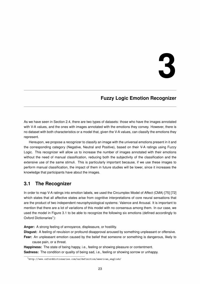
3Fuzzy Logic Emotion Recognizer

As we have seen in Section 2.4, there are two types of datasets: those who have the images annotatedwith V-A values, and the ones with images annotated with the emotions they convey. However, there isno dataset with both characteristics or a model that, given the V-A values, can classify the emotions theyrepresent.

Hereupon, we propose a recognizer to classify an image with the universal emotions present in it andthe corresponding category (Negative, Neutral and Positive), based on their V-A ratings using FuzzyLogic. This recognizer will allow us to increase the number of images annotated with their emotionswithout the need of manual classification, reducing both the subjectivity of the classification and theextensive use of the same stimuli. This is particularly important because, if we use these images toperform manual classification, the impact of them in future studies will be lower, since it increases theknowledge that participants have about the images.

3.1 The Recognizer

In order to map V-A ratings into emotion labels, we used the Circumplex Model of Affect (CMA) [75] [72]which states that all affective states arise from cognitive interpretations of core neural sensations thatare the product of two independent neurophysiological systems: Valence and Arousal. It is important tomention that there are a lot of variations of this model with no consensus among them. In our case, weused the model in Figure 3.1 to be able to recognize the following six emotions (defined accordingly toOxford Dictionaries1):

Anger: A strong feeling of annoyance, displeasure, or hostility.Disgust: A feeling of revulsion or profound disapproval aroused by something unpleasant or offensive.Fear: An unpleasant emotion caused by the belief that someone or something is dangerous, likely to

cause pain, or a threat.Happiness: The state of being happy, i.e., feeling or showing pleasure or contentment.Sadness: The condition or quality of being sad, i.e., feeling or showing sorrow or unhappy.

1http://www.oxforddictionaries.com/us/definition/american_english/

23

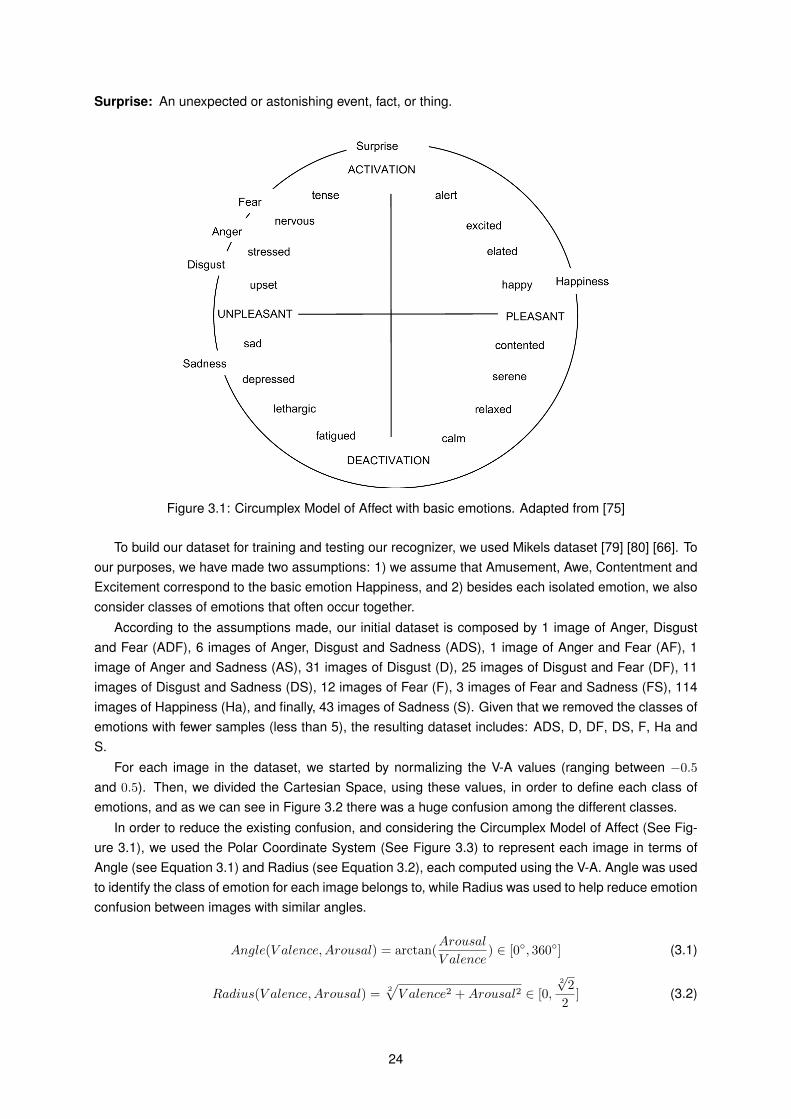
Surprise: An unexpected or astonishing event, fact, or thing.

Figure 3.1: Circumplex Model of Affect with basic emotions. Adapted from [75]

To build our dataset for training and testing our recognizer, we used Mikels dataset [79] [80] [66]. Toour purposes, we have made two assumptions: 1) we assume that Amusement, Awe, Contentment andExcitement correspond to the basic emotion Happiness, and 2) besides each isolated emotion, we alsoconsider classes of emotions that often occur together.

According to the assumptions made, our initial dataset is composed by 1 image of Anger, Disgustand Fear (ADF), 6 images of Anger, Disgust and Sadness (ADS), 1 image of Anger and Fear (AF), 1image of Anger and Sadness (AS), 31 images of Disgust (D), 25 images of Disgust and Fear (DF), 11images of Disgust and Sadness (DS), 12 images of Fear (F), 3 images of Fear and Sadness (FS), 114images of Happiness (Ha), and finally, 43 images of Sadness (S). Given that we removed the classes ofemotions with fewer samples (less than 5), the resulting dataset includes: ADS, D, DF, DS, F, Ha andS.

For each image in the dataset, we started by normalizing the V-A values (ranging between �0.5

and 0.5). Then, we divided the Cartesian Space, using these values, in order to define each class ofemotions, and as we can see in Figure 3.2 there was a huge confusion among the different classes.

In order to reduce the existing confusion, and considering the Circumplex Model of Affect (See Fig-ure 3.1), we used the Polar Coordinate System (See Figure 3.3) to represent each image in terms ofAngle (see Equation 3.1) and Radius (see Equation 3.2), each computed using the V-A. Angle was usedto identify the class of emotion for each image belongs to, while Radius was used to help reduce emotionconfusion between images with similar angles.

Angle(V alence,Arousal) = arctan(Arousal

V alence) 2 [0�, 360�] (3.1)

Radius(V alence,Arousal) = 2pV alence2 +Arousal2 2 [0,

2p2

2] (3.2)

24

Figure 3.2: Distribution of the images in terms of Valence and Arousal

Figure 3.3: Polar Coordinate System for the distribution of the images

25

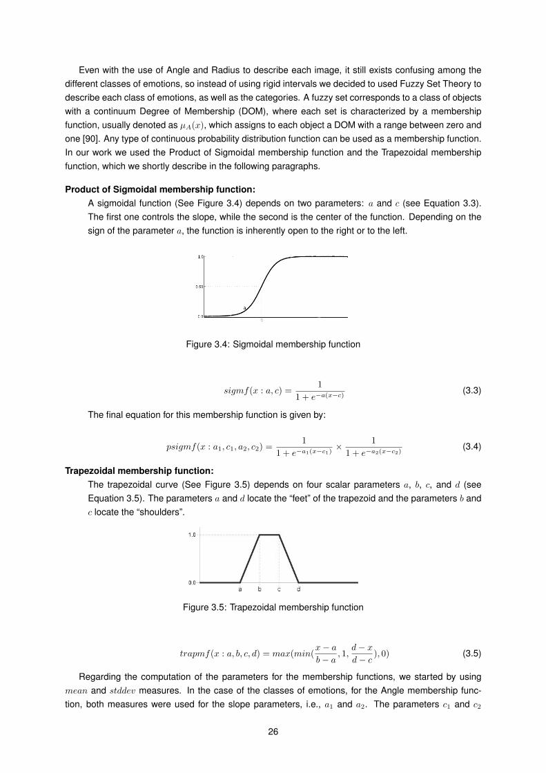
Even with the use of Angle and Radius to describe each image, it still exists confusing among thedifferent classes of emotions, so instead of using rigid intervals we decided to used Fuzzy Set Theory todescribe each class of emotions, as well as the categories. A fuzzy set corresponds to a class of objectswith a continuum Degree of Membership (DOM), where each set is characterized by a membershipfunction, usually denoted as µ

A

(x), which assigns to each object a DOM with a range between zero andone [90]. Any type of continuous probability distribution function can be used as a membership function.In our work we used the Product of Sigmoidal membership function and the Trapezoidal membershipfunction, which we shortly describe in the following paragraphs.

Product of Sigmoidal membership function:A sigmoidal function (See Figure 3.4) depends on two parameters: a and c (see Equation 3.3).The first one controls the slope, while the second is the center of the function. Depending on thesign of the parameter a, the function is inherently open to the right or to the left.

Figure 3.4: Sigmoidal membership function

sigmf(x : a, c) =1

1 + e�a(x�c)(3.3)

The final equation for this membership function is given by:

psigmf(x : a1, c1, a2, c2) =1

1 + e�a1(x�c1)⇥ 1

1 + e�a2(x�c2)(3.4)

Trapezoidal membership function:The trapezoidal curve (See Figure 3.5) depends on four scalar parameters a, b, c, and d (seeEquation 3.5). The parameters a and d locate the “feet” of the trapezoid and the parameters b andc locate the “shoulders”.

Figure 3.5: Trapezoidal membership function

trapmf(x : a, b, c, d) = max(min(x� a

b� a, 1,

d� x

d� c), 0) (3.5)

Regarding the computation of the parameters for the membership functions, we started by usingmean and stddev measures. In the case of the classes of emotions, for the Angle membership func-tion, both measures were used for the slope parameters, i.e., a1 and a2. The parameters c1 and c2

26

correspond, respectively, to the lowest and highest value of the Angle for that subset of images. For theRadius membership function, b is the minimum, and c the maximum value of the Radius for that subsetof images, while a = b � ✏1 and d = c + ✏2, with ✏1 = ✏2 = 0.01 (empirical value). In the case of thecategories parameters, and since we used trapezoidal memberships for the angles and the radiuses,b and c parameters correspond to the lowest and highest value of the Angle/Radius for that subset ofimages; in the case of the parameters a and d, the only difference are the ✏ values that vary accordingto each category. For all the classes of emotions, we removed the outliers, i.e, images with angles orradius that were distant from the angles or radius of the majority of the images for the correspondingclass.

Although fuzzy sets are commonly defined using only one dimension, they can be complementedwith the use of cylindrical extensions. Given this, we used a two-dimensional membership function thatis the result of the composition of the two one-dimensional membership functions mentioned above.

For each category (see Figure 3.7 to 3.11) we used Trapezoidal membership function, both forAngle and Radius (see Equation 3.6). In the case of the classes of emotions (see Figures 3.12 to 3.18)we used the Product of Sigmoidal membership function for the Angle and the Trapezoidal membershipfunction for the Radius (see Equation 3.7).

category(Angle,Radius : a1, c1, a2, c2, a, b, c, d) = trapmf(Angle : a, b, c, d)

⇥trapmf(Radius : a, b, c, d)(3.6)

emotions(Angle,Radius : a1, c1, a2, c2, a, b, c, d) = psigmf(Angle : a1, c1, a2, c2)

⇥trapmf(Radius : a, b, c, d)(3.7)

2-D Membership Function

27

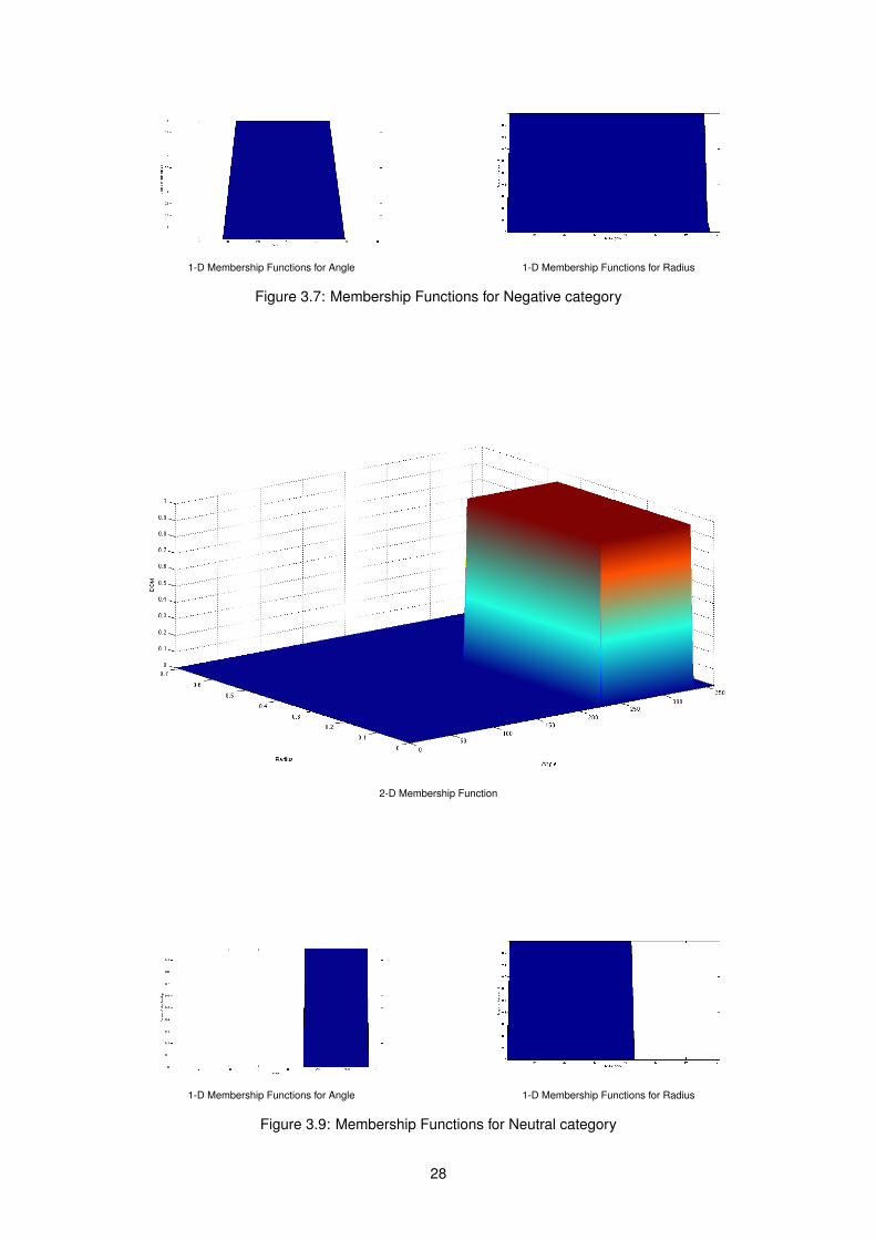
1-D Membership Functions for Angle 1-D Membership Functions for Radius

Figure 3.7: Membership Functions for Negative category

2-D Membership Function

1-D Membership Functions for Angle 1-D Membership Functions for Radius

Figure 3.9: Membership Functions for Neutral category

28

2-D Membership Function

1-D Membership Functions for Angle 1-DMembership Functions for Radius

Figure 3.11: Membership Functions for Positive category

2-D Membership Function

29

1-D Membership Function for Angle 1-D Membership Function for Radius

Figure 3.12: Membership Functions for Anger, Disgust and Sadness

2-D Membership Function

1-D Membership Function for Angle 1-D Membership Function for Radius

Figure 3.13: Membership Functions for Disgust

30

2-D Membership Function

1-D Membership Function for Angle 1-D Membership Function for Radius

Figure 3.14: Membership Functions for Disgust and Fear

2-D Membership Function

31

1-D Membership Function for Angle 1-D Membership Function for Radius

Figure 3.15: Membership Functions for Disgust and Sadness

2-D Membership Function

1-D Membership Function for Angle 1-D Membership Function for Radius

Figure 3.16: Membership Functions for Fear

32

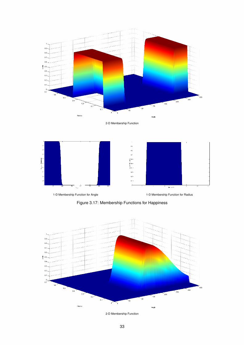
2-D Membership Function

1-D Membership Function for Angle 1-D Membership Function for Radius

Figure 3.17: Membership Functions for Happiness

2-D Membership Function

33

1-D Membership Function for Angle 1-D Membership Function for Radius

Figure 3.18: Membership Functions for Sadness

Each image was annotated with the degree of membership for each possible category and class ofemotions, and were also associated to the image the two dominant categories and the two dominantclasses of emotions.

In Figure 3.19 there is a global view of the membership functions of all the classes of emotions forAngle, being possible to see the existing confusion between each of the classes of emotions. Thereis clearly a differentiation between the Positive emotion Happiness, ([0�, 95�] [ [300�, 360�]) and theNegative emotions ([120�, 280�]). However, there is a lot of confusion among the Negative emotions,being the main confusions between DF and F, between D, DF, ADS and DS, and finally between ADS,DS and S. With the exception of DF, that is overlapping with almost all other Negative emotions, evenwith the ones without any obvious connection (for example S), the remaining are logical, and expectable,overlaps of emotions.

Figure 3.19: Membership Functions of Angle for all classes of emotions

34

In Figure 3.20 there is a global view of the confusion between emotions regarding Radius. In thiscase, and contrary to what happened in the case of Angle, there is no clear differentiation betweenNegative and Positive emotions. As we can see, there are no emotions in the proximity of the extremes(0 and 70), in fact the emotions are lying between 8 and 55. Almost all emotions are completely insidethe D interval ([10, 55]), which is the emotion with the biggest range of values for Radius. In some cases,such as F, which is completely inside DF, or S, which almost overlaps completely DF, the Radius willnot be particularly helpful. However, and considering the results for the Angle, in the case of confusionsbetween ADS, DS and S, the use of Radius will be useful, for example in the interval of [10, 18] theemotion will undoubtedly be S. So, the combination of the two attributes (Angle and Radius) allow us tobetter distinguish the emotions.

Figure 3.20: Membership Functions of Radius for all classes of emotions

3.2 Experimental Results

In order to build the training dataset, we analyzed the dataset for each class of emotions and categories.For both cases, we concluded that the distribution of the images is not symmetric, being more evident inthe classes of emotions.

For the proper evaluation of our model for the classes of emotions, and taking into account that“Clinicians and researchers have long noted the difficulty that people have in assessing, discerning,and describing their own emotions. This difficulty suggests that individuals do not experience, or recog-nize, emotions as isolated, discrete entities, but that they rather recognize emotions as ambiguous andoverlapping experiences.” as stated in [72], we consider that a result is correct if the expected class ofemotion is present (totally or partially) in the result label; if it is not present, we consider the class ofemotion with the biggest DOM as a confusion. For example, if the expected class of emotion was D, weconsidered correct results ADS, DS, D, DF or any combination of one of those with a second class ofemotion.

As we can see in Table 3.1, the best results were achieved for D, F and Ha. In the case of Ha, thisresult is due to the clear distinction between the Angle values for Ha and the remaining emotions; while

35

in the case of D, we believe it is due to the big interval, both for Angle and Radius; finally, in the case ofF, we believe it is because of the interval of Angle that is only overlapping with DF. However, DF showsthe worst result, but this is expectable given that both the Angle and Radius intervals are overlappingwith the majority of the emotions.

(%) ADS D DF DS F S HADS 83.33 16.67

D 100DF 76 8 16DS 9.09 90.91F 100S 4.65 4.65 90.70H 100

Table 3.1: Confusion Matrix for the classes of emotions in the IAPS dataset

For evaluating the model when it come to categories, we follow a similar approach to the one de-scribed above. If the expected category is one of the returned categories, we consider the result ascorrect; otherwise we consider the one with the biggest DOM as a confusion. If the two categories havethe same DOM we select the “worst”, i.e., for example between Neutral and Positive, we choose Neutralas the confusion result. Table 3.2 presents the achieved results for the IAPS dataset (correspondingto our training dataset), while Table 3.3 shows the results for the GAPED dataset. These results wereachieved after the adjustment of the Radius parameters for each category (in order to eliminate somenon-classified results).

(%) Negative PositiveNegative 100Positive 100

Table 3.2: Confusion Matrix for the categories in the Mikels dataset

(%) Negative Neutral PositiveNegative 87.89 7.69 4.42Neutral 98.88 1.12Positive 100

Table 3.3: Confusion Matrix for the categories in the GAPED dataset

As expected the results achieved when using the same set for training and test were 100% forNegative and Positive categories. With the use of GAPED as a testing set and with the addition ofthe Neutral category (which did not exist in the training dataset), the results for the Negative categorybecame worse; however, this is mainly due to the existing confusion between the Negative and Neutralcategories in the used dataset [14]. The Positive category maintains an accuracy of 100%, while theNeutral category obtained almost 99%.

3.3 Discussion

In this work, we developed a model to automatically classify the emotions and categories conveyed byan image in terms of their normalized Valence and Arousal ratings. With this model we were able tosuccessfully annotate our training set with the dominant categories with classification rates of 100% andthe dominant classes of emotions with an average classification rate of 91.56%.

36

Although we intend to be able to recognize the six basic emotions, we don’t have any data for theemotions of Anger and Surprise. In the case of Anger, this is due to the fact that it is difficult to elicit theemotion through the images used as explained in [66], while in the case of the emotion Surprise, it isbecause the work we followed did not consider this emotion.

In general, the results achieved are very good; however, in the case of emotions, it is importantto mention the existing confusion between some of them, mainly Disgust and Sadness (and the corre-sponding classes that are composed with at least one of these emotions), which can be explained by theneuroanatomical findings in [48], in which the authors mentioned that some regions such as prefrontalcortex and thalamus are common to these emotions, as well as the association with activation of anteriorand posterior temporal structures of the brain, using film-induced emotion.

We also annotated the GAPED dataset and the remaining pictures of the IAPS dataset. For GAPEDwe have a non-classification rate of 23.4%, and an average classification rate of 95.59% for the cate-gories (we don’t have any information about the emotions). In the case of IAPS we achieved a non-classification rate of 4.86%, however we cannot identify the classification rates because, besides theimages we used as training set (Mikels), we did not have any information about the categories or emo-tions. The non-classified results are explained with the lack of images covering the whole space of theCMA on both datasets, and, in the particular case of GAPED it can also be explained by the use ofa slightly different CMA. The existing confusion between the Negative and Neutral categories (in theGAPED dataset) already existed as explained in [14], while the confusion between the Negative andPositive categories can be explained by the use of different models of the CMA.

3.4 Summary

We developed a recognizer to classify an image with the universal emotions present in it and the corre-sponding category (Negative, Neutral and Positive), based on their V-A ratings using Fuzzy Logic. Foreach image in the dataset, we started by normalizing the V-A values, and computed the Angle and theRadius for each image in order to help reduce emotion confusion between images with similar angles.

To describe each class of emotions, as well as the categories, we used the Product of Sigmoidalmembership function and the Trapezoidal membership function. For the categories we used Trapezoidalmembership function, both for Angle and Radius, while for the classes of emotions, we used the Productof Sigmoidal membership function for the Angle and the Trapezoidal membership function for the Radius;

As expected, the results achieved when using the same set for training and test were 100% forNegative and Positive categories. In the case of the dominant classes of emotions we achieved anaverage classification rate of 91.56%. With the use of GAPED as a testing set we achieved an averagerecognition rate of 96% for categories. For GAPED, we achieved a non-classification rate of 23.4%,while in the case of the IAPS, we achieved a non-classification rate of 4.86%.

37

38

4Content-Based Emotion Recognizer

Emotion, which is also called mood or feeling, can be seen as emotional content of an image itselfor the impression it makes on a human. When talking about emotions, it is important to mention thesubjectivity inherent, since different emotions can appear in a subject while looking at the same picture,depending on its current emotional state [67]. However, the expected affective response can be con-sidered objective, as it reflects the more-or-less unanimous response of a general audience to a givenstimulus [30].

There is a general agreement on the fact that humans can perceive all levels of image features,from the primitive/syntactic to the highly semantic ones [74], and also that artists have been exploringthe formal elements of art, such as lines, space, mass, light or color to express emotions [18]. Giventhis, we assumed that emotional content can be characterized by the image color, texture and shape.Additionally, and given that certain features in photographic images are believed, by many, to pleasehumans more than others, we also consider the aesthetics of an image, that in the world of art andphotography refers to the principles of the nature and appreciation of beauty [17,39].

In order to acquire as much information as possible about an image, we will use different featuresregarding Color, Texture, Shape, Composition, among others. However, a commitment between all theinformation collected and the processing time has to be found. Since most of the descriptors only modela particular property of the images, and in order to obtain the best results, a combination of features isoften required. As stated in [30, 74], low-level image features can be easily extracted using computervision methods, however they are no match for the information a human observer perceives.

After the identification of the features that can be used to describe an image in terms of their emo-tional content, we will train different classifiers in order to identify the best features to describe an imageaccording to their category of emotions. Given this, our goal is to identify the combination of visual fea-tures that can match human perception as closely as possible regarding the Positive or Negative contentof an image.

Regarding the features’ extraction, we selected the most used in literature and easiest to com-pute resulting in the following descriptor vector features (for simplification purposes, in the future, wewill only refer to them as “features”): AutoColorCorrelogram (ACC) [36], Color Histogram (CH) [78],Color Moments (CM) [17], Number of Different Colors (NDC) [18], Opponent Histogram (OH) [85],

39

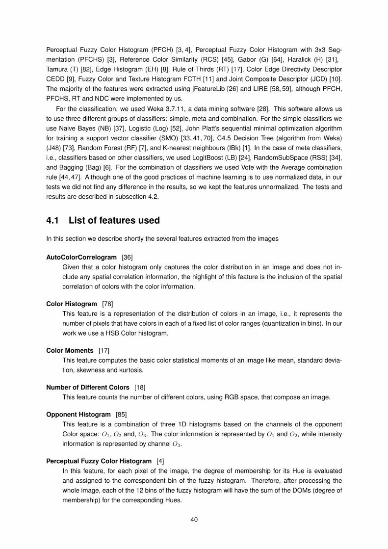
Perceptual Fuzzy Color Histogram (PFCH) [3, 4], Perceptual Fuzzy Color Histogram with 3x3 Seg-mentation (PFCHS) [3], Reference Color Similarity (RCS) [45], Gabor (G) [64], Haralick (H) [31],Tamura (T) [82], Edge Histogram (EH) [8], Rule of Thirds (RT) [17], Color Edge Directivity DescriptorCEDD [9], Fuzzy Color and Texture Histogram FCTH [11] and Joint Composite Descriptor (JCD) [10].The majority of the features were extracted using jFeatureLib [26] and LIRE [58, 59], although PFCH,PFCHS, RT and NDC were implemented by us.

For the classification, we used Weka 3.7.11, a data mining software [28]. This software allows usto use three different groups of classifiers: simple, meta and combination. For the simple classifiers weuse Naive Bayes (NB) [37], Logistic (Log) [52], John Platt’s sequential minimal optimization algorithmfor training a support vector classifier (SMO) [33, 41, 70], C4.5 Decision Tree (algorithm from Weka)(J48) [73], Random Forest (RF) [7], and K-nearest neighbours (IBk) [1]. In the case of meta classifiers,i.e., classifiers based on other classifiers, we used LogitBoost (LB) [24], RandomSubSpace (RSS) [34],and Bagging (Bag) [6]. For the combination of classifiers we used Vote with the Average combinationrule [44, 47]. Although one of the good practices of machine learning is to use normalized data, in ourtests we did not find any difference in the results, so we kept the features unnormalized. The tests andresults are described in subsection 4.2.

4.1 List of features used

In this section we describe shortly the several features extracted from the images

AutoColorCorrelogram [36]Given that a color histogram only captures the color distribution in an image and does not in-clude any spatial correlation information, the highlight of this feature is the inclusion of the spatialcorrelation of colors with the color information.

Color Histogram [78]This feature is a representation of the distribution of colors in an image, i.e., it represents thenumber of pixels that have colors in each of a fixed list of color ranges (quantization in bins). In ourwork we use a HSB Color histogram.

Color Moments [17]This feature computes the basic color statistical moments of an image like mean, standard devia-tion, skewness and kurtosis.

Number of Different Colors [18]This feature counts the number of different colors, using RGB space, that compose an image.

Opponent Histogram [85]This feature is a combination of three 1D histograms based on the channels of the opponentColor space: O1, O2 and, O3. The color information is represented by O1 and O2, while intensityinformation is represented by channel O3.

Perceptual Fuzzy Color Histogram [4]In this feature, for each pixel of the image, the degree of membership for its Hue is evaluatedand assigned to the correspondent bin of the fuzzy histogram. Therefore, after processing thewhole image, each of the 12 bins of the fuzzy histogram will have the sum of the DOMs (degree ofmembership) for the corresponding Hues.

40

Perceptual Fuzzy Color Histogram with 3x3 Segmentation [3]This feature divides an image into 9 equal parts, and performs PFCH in each one. The result isthe combination of the nine fuzzy histograms.

Reference Color Similarity [45]This feature is not a histogram, since reference colors used are processed independently; anysubset of dimensions gives the same result as computing just these colors, making this featurespace very favorable for feature bagging and other projections.

Gabor [64]This feature represents and discriminates Texture information, using frequency and orientationrepresentations of Gabor filters since they are similar to those of the human visual system.

Haralick [31]This feature is based on statistics, and summarizes the relative frequency distribution, that de-scribes how often one gray tone will appear in a specified spatial relationship to another gray toneon the image.

Tamura [82]This feature implements three of the following Tamura features: coarseness, contrast, directionality,line-likeness, regularity and roughness.

Edge Histogram [8]This feature captures the spatial distribution of undirected edges within an image. The imageis divided into 16-equal-sized, non overlapping blocks. After that, each block is divided into a5-bin histogram counting edges in the following categories: vertical, horizontal, 35�, 135�and non-directional.

Rule of Thirds [17]This feature computes the color moments for the inner rectangle of an image divided into 9 equalparts.

Color Edge Directivity Descriptor [9]This feature incorporates Color and Texture information in a histogram. In order to extract the Colorinformation, it uses a Fuzzy-Linking histogram. Texture information is captured using 5 digital filtersthat were proposed in the MPEG-7 Edge Histogram Descriptor.

Fuzzy Color and Texture Histogram [11]This feature combines, in one histogram, Color and Texture information using 3 fuzzy systems.

Joint Composite Descriptor [10]This feature corresponds to a joint descriptor that joins CEDD and FCTH information in one his-togram.

4.2 Classifier

For testing and training, we used Mikels dataset [66,79,80], with 113 Positive images and 123 Negativeimages. The Positive images are the ones with the Happiness label, while the Negative ones correspondto ADS (6), D (31), DF (20), DS (11), F (12) and S (43) labels. We separated the data into a training andtest set using K-fold Cross Validation with K = 5 [60].

We started by analyzing a set of classifiers, in order to understand which one learned best the relationbetween features and the given category of emotion (See Table A1). In the case of the simple classifiers

41

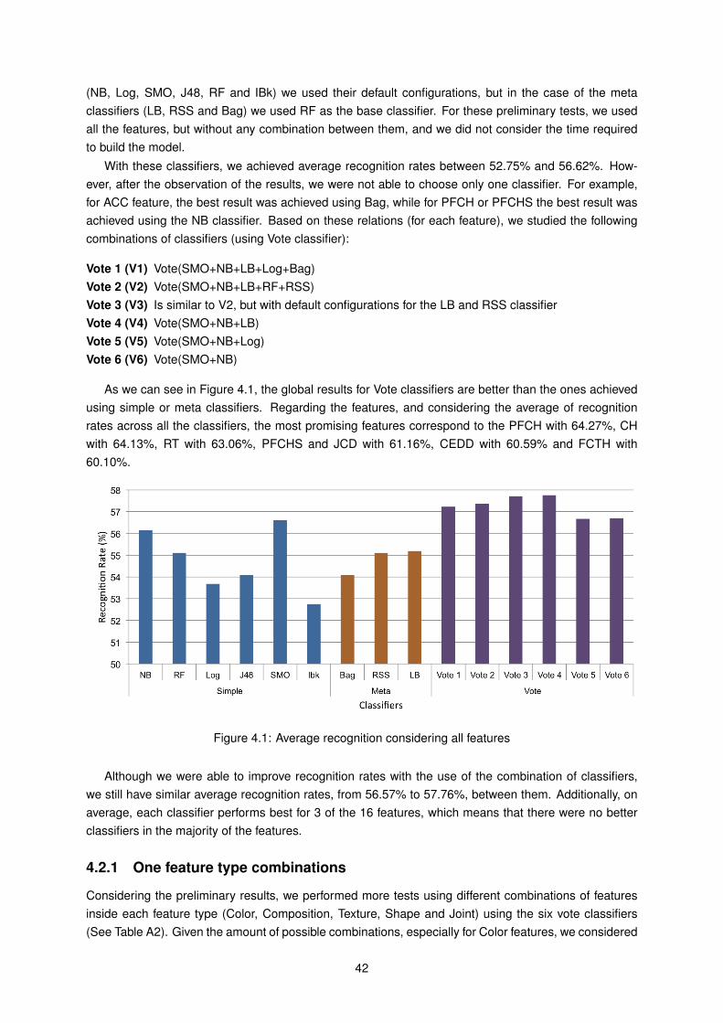
(NB, Log, SMO, J48, RF and IBk) we used their default configurations, but in the case of the metaclassifiers (LB, RSS and Bag) we used RF as the base classifier. For these preliminary tests, we usedall the features, but without any combination between them, and we did not consider the time requiredto build the model.

With these classifiers, we achieved average recognition rates between 52.75% and 56.62%. How-ever, after the observation of the results, we were not able to choose only one classifier. For example,for ACC feature, the best result was achieved using Bag, while for PFCH or PFCHS the best result wasachieved using the NB classifier. Based on these relations (for each feature), we studied the followingcombinations of classifiers (using Vote classifier):

Vote 1 (V1) Vote(SMO+NB+LB+Log+Bag)Vote 2 (V2) Vote(SMO+NB+LB+RF+RSS)Vote 3 (V3) Is similar to V2, but with default configurations for the LB and RSS classifierVote 4 (V4) Vote(SMO+NB+LB)Vote 5 (V5) Vote(SMO+NB+Log)Vote 6 (V6) Vote(SMO+NB)

As we can see in Figure 4.1, the global results for Vote classifiers are better than the ones achievedusing simple or meta classifiers. Regarding the features, and considering the average of recognitionrates across all the classifiers, the most promising features correspond to the PFCH with 64.27%, CHwith 64.13%, RT with 63.06%, PFCHS and JCD with 61.16%, CEDD with 60.59% and FCTH with60.10%.

Figure 4.1: Average recognition considering all features

Although we were able to improve recognition rates with the use of the combination of classifiers,we still have similar average recognition rates, from 56.57% to 57.76%, between them. Additionally, onaverage, each classifier performs best for 3 of the 16 features, which means that there were no betterclassifiers in the majority of the features.

4.2.1 One feature type combinations

Considering the preliminary results, we performed more tests using different combinations of featuresinside each feature type (Color, Composition, Texture, Shape and Joint) using the six vote classifiers(See Table A2). Given the amount of possible combinations, especially for Color features, we considered

42

as candidates for the best features those with a recognition rate greater than the average of all thefeatures (for each classifier).

Color

In Table A3, we can see the results for Color using only one feature. Tables A4 to Table A10 show theresults for combinations of two to all of the Color features. The grey cells in tables correspond to thecells with a value greater than the average for that classifier. In the following paragraphs we discuss theresults for the various combinations of features.

One feature:Even though we had only identified the Color features PFCH, PFCHS and CH, earlier, as themost promising, we also included OH and RCS to the Color candidates list. As expected from theliterature, and as we can see in Figure 4.2 the best results were the ones corresponding to anytype of histogram, in particular the commonly used Color Histogram, as well as PFCH and PFCHS,that take into account the way users perceive color.

Figure 4.2: Results for Color - one feature

Two features:When we considered combinations of two Color features, the average recognition rates increasedalmost 2%, considering all of the possible combinations. As we can see in figure 4.3 the bestresults were achieved using combinations that include CH, PFCHS or PFCH.

Generally, for CH, the use of NDC, OH, PFCH and RCS improved its recognition rates, while CMand PFCHS reduced them. The features OH and NDC, when combined with the other features,also improved their average recognition rate. Finally, PFCH is improved slightly when combined

43

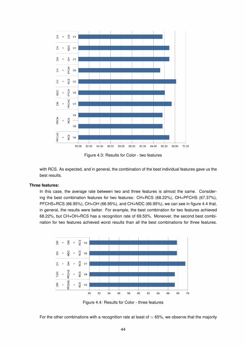
Figure 4.3: Results for Color - two features

with RCS. As expected, and in general, the combination of the best individual features gave us thebest results.

Three features:In this case, the average rate between two and three features is almost the same. Consider-ing the best combination features for two features: CH+RCS (68.22%), OH+PFCHS (67.37%),PFCHS+RCS (66.95%), CH+OH (66.95%), and CH+NDC (66.95%), we can see in figure 4.4 that,in general, the results were better. For example, the best combination for two features achieved68.22%, but CH+OH+RCS has a recognition rate of 69.50%. Moreover, the second best combi-nation for two features achieved worst results than all the best combinations for three features.

Figure 4.4: Results for Color - three features

For the other combinations with a recognition rate at least of ' 65%, we observe that the majority

44

of them achieved better results than the ones achieved only with the use of two features. However,for example, CH+OH+PFCH has a rate of 65.68% while CH+OH has a better rate of 66.95%.These observations allow us to conclude, for now, and against our beliefs, that with the increaseof information, in general, the accuracy of the classification is not linearly better.

Four features:Contrary to what happened in the previously analyzed tests, the average rate between three andfour features has decreased. The same also happened if we consider only the average for the bestfeatures. Although the differences appears to be minimal, nevertheless they meet our previousobservation. The best results were the ones including the combination CH+CM+NDC, where thebest combination was CH+CM+NDC+RCS with a recognition rate of 68.64% using V2.

Five features:Comparing these tests with the ones above, we noticed a marginal decrease in the average recog-nition rate for all combinations. Just by looking to the best features: CH+CM+NDC+OH+RCS(67.80%), and CH+CM+NDC+OH+PFCHS (66.95%), we found the contrary since there was asmall increase, in the recognition rate, when compared with CH+CM+NDC+OH (66.10%).

For all the combinations based on CM+NDC+OH+PFCH or NDC+OH+PFCH+PFCHS, in general,there were no noticeable differences in the average recognition rates when compared with theresults from five features. But when we combined them with the RCS feature we verified anincrease in the corresponding recognition rates.

Six features:CH+CM+NDC+OH+PFCH+RCS (67.80%), and CH+CM+NDC+OH+PFCH+PFCHS (67.38%) werethe best combinations. In both cases, when we compared them with CH+CM+NDC+OH+PFCH(65.25%) there was a significant improvement in the recognition rates achieved.

In some cases, such as for example CM+NDC+OH+PFCH+PFCHS or CH+CM+NDC+OH+PFCH,if we combine them with the RCS feature, there was an improvement in the corresponding averagerecognition rates.

Seven features:In this group we achieved a poor average recognition rate. However, this was expectable since themajority of the combinations include the ACC feature. This feature had achieved the worst resultsin all the performed tests. The best combination was CH+CM+NDC+OH+PFCH+PFCHS+RCSthat achieved an average recognition rate of 66.95% for V3.

All features:Across all the tests, this was one of the worst results. However, as in the previous test this wasexpectable since it includes the worst feature (ACC). In fact, as we can see in Table A9, the samecombination without ACC feature has an average rate of 64.69%.

In Table A11, there is the final list of Color candidate features. Given the size of this list, we startedby reducing the number of classifiers to analyze. We first looked into the recognition rates for all thecombinations for each of the classifiers. V4 was the best classifier with an average rate of 63.96%,followed by V1, V2, V3, V5, and V6, with similar recognition rates of 63.83%, 63.71%, 63.62%, 62.70%,and 62.19%. Given these results, we only kept analyzing the values for the best classifiers, i.e., V4, V1and V2, and decided to keep only Color combinations with an average recognition rate of at least 66%,reducing the list only to 7 combinations of features (See Table 4.1).

45

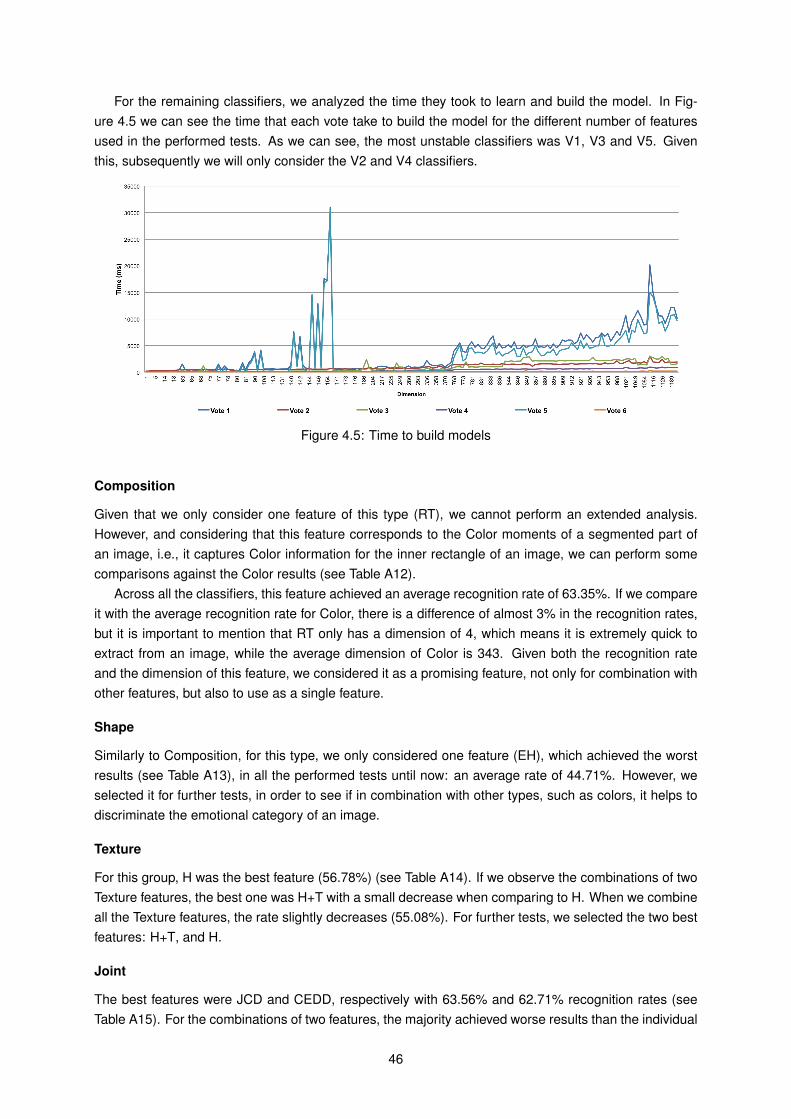
For the remaining classifiers, we analyzed the time they took to learn and build the model. In Fig-ure 4.5 we can see the time that each vote take to build the model for the different number of featuresused in the performed tests. As we can see, the most unstable classifiers was V1, V3 and V5. Giventhis, subsequently we will only consider the V2 and V4 classifiers.

Figure 4.5: Time to build models

Composition

Given that we only consider one feature of this type (RT), we cannot perform an extended analysis.However, and considering that this feature corresponds to the Color moments of a segmented part ofan image, i.e., it captures Color information for the inner rectangle of an image, we can perform somecomparisons against the Color results (see Table A12).

Across all the classifiers, this feature achieved an average recognition rate of 63.35%. If we compareit with the average recognition rate for Color, there is a difference of almost 3% in the recognition rates,but it is important to mention that RT only has a dimension of 4, which means it is extremely quick toextract from an image, while the average dimension of Color is 343. Given both the recognition rateand the dimension of this feature, we considered it as a promising feature, not only for combination withother features, but also to use as a single feature.

Shape

Similarly to Composition, for this type, we only considered one feature (EH), which achieved the worstresults (see Table A13), in all the performed tests until now: an average rate of 44.71%. However, weselected it for further tests, in order to see if in combination with other types, such as colors, it helps todiscriminate the emotional category of an image.

Texture

For this group, H was the best feature (56.78%) (see Table A14). If we observe the combinations of twoTexture features, the best one was H+T with a small decrease when comparing to H. When we combineall the Texture features, the rate slightly decreases (55.08%). For further tests, we selected the two bestfeatures: H+T, and H.

Joint

The best features were JCD and CEDD, respectively with 63.56% and 62.71% recognition rates (seeTable A15). For the combinations of two features, the majority achieved worse results than the individual

46

ones, with the exception of the FCTH+JCD that had the same rate as CEDD. For the combination ofall the features we achieved an average recognition rate of 61.44%. The selected features were: JCD(61.16%), CEDD, and FCTH+JCD.

In Table 4.1 we can see the final list of features to use in the following tests. Regarding the distributionof the type of features, we have 50.00% for Color features, 21.44% for Joint, 14.28% for Texture, and theremaining 14.28% equally divided between Composition and Shape features.

At this point, and given these results, we expect that the combination of features of different typesincreases the recognition rates, and allows us to better discriminate the emotional category of a givenimage. The new tests were done using combinations of two and three different types of features.

Color

CH+RCSCH+NDC+RCSCH+OH+RCSCH+PFCH+RCSCH+PFCHS+RCSCH+CM+NDC+RCSCH+CM+NDC+OH+PFCH+RCS

Composition RTShape EH

Texture HH+T

JointCEDDJCDFCTH+JCD

Table 4.1: List of best features for each category type

4.2.2 Two feature type combinations

In the case of the tests performed using combinations of two types of features, the results can be seen inTable A16 for Color and Composition, Table A17 for Color and Shape, Table A18 for Color and Texture,Table A19 for Color and Joint, Table A20 for Composition and Shape, Table A21 for Composition andTexture, Table A22 for Composition and Joint, Table A23 for Shape and Texture, Table A24 for Shapeand Joint, and Table A25 for Texture and Joint.

Using the combination of the best features for Color and Composition, almost all the combinationsperformed worse than the original feature Color (i.e., without the Composition feature); the only exceptionwas OH+PFCHS+RCS+RT which increased the corresponding recognition rate. In the case of Color andShape, with the addition of Color information to the Shape features, all the combinations achieved betterresults. For Color and Texture, some of the Color combinations were improved with the use of theTexture feature H, namely CH+PFCH+RCS and CH+PFCHS+RCS. In fact, CH+PFCH+RCS+H, is oneof the best features. Regarding the two Texture features used: H and H+T, the first one when combinedwith the different feature colors achieved, on average, better results. In the tests using Color and Joint,we were combining two of the best feature types. None of the combinations performed better than theoriginal Color feature, which means that the use of CEDD, JCD, and FCTH+JCD did not add any usefulinformation to the one already captured by color.

For the combination of Composition and Shape, if we compare it with Shape feature EH, it is slightlybetter, however it is considerably worse (more than 13%) if compared with the Composition feature RT.On average, the achieved results using combined Composition and Texture features were worse thanthe average recognition rate of the two types separately. In the case of the Texture feature H+T, it is

47

slightly better when combined with RT, with a similar dimension, which means that, in this case, it isbetter to use the combined feature. For Composition and Joint, all of the combinations achieved worseresults than the isolated features. So, in this case it is preferable to use Composition feature alone.

Regarding Shape and Texture, and although the tested combinations achieved a better averagerecognition rate when compared to Shape, it is still better to use one of the Texture features (H or H+T),since the corresponding recognition remains better. For Shape and Joint combinations, when comparedwith Shape the achieved results were better, but considerably lower than the results achieved for Joint.In the case of Texture and Joint all of the combinations, when compared with Texture features, wereimproved.

4.2.3 Three feature type combinations

For the tests using combinations of three types of features, the results are in Table A26 for Color, Com-position and Shape, Table A27 for Color, Composition and Texture, Table A28 for Color, Compositionand Joint, Table A29 for Color, Shape and Texture, Table A30 for Color, Shape and Joint, and Table A31for Color, Texture and Joint.

For Color, Composition and Shape, all the combinations achieved worst results with the additionof Shape feature. For Color, Composition and Texture, with the addition of Texture information toColor and Composition combinations, some of the new combinations achieved better results such asOH+PFCHS+RCS+RT+H or OH+PFCHS+RCS+RT+H+T. For Color, Composition and Joint all the re-sults were worst. In the case of Color and Shape and Texture we achieved better recognition rates,especially with the use of H Texture feature. For Color, Shape and Joint, we achieved some betterresults with the use of FCTH+JCD feature. For Color, Texture and Joint all the results were worst.

In general, the results with the addition of more information tend to decrease, even though wewere able to improve some of our previous results. Considering the results achieved until now, forthe next tests we will only use the best three feature type combinations: OH+PFCHS+RCS+RT+H,OH+PFCHS+RCS+RT+H+T, CH+RCS+H+FCTH+JCD, and CH+PFCH+RCS+H+T+CEDD.

4.2.4 Four feature type combinations

For these tests, the results can be seen in Table A32 for Color, Composition, Texture and Shape, Ta-ble A33 for Color, Composition, Texture and Joint, Table A34 for Color, Texture, Joint and Shape, and inTable A35 for Color, Texture, Joint and Composition.

For all the combinations, the achieved results were considerably worse than the original ones. Theaverage recognition rate of the initial combinations was 66.53%, while the new achieved recognitionrate decreased to 62.83%. Given these results, we will not perform tests using all the feature typescombinations.

4.2.5 Overall best features combinations

In Table 4.2 we can see the best features across all the tests, and the recognition rates achieved.

% V2 V4

Color CH + OH + RCS 68.64 66.53CH + CM + NDC + RCS 68.64 66.10

Color and Composition CH + OH + RCS + RT 67.37 64.83CH + CM + NDC + RCS + RT 66.95 65.25

Color and Texture

CH + RCS + H 67.80 64.83CH + PFCH + RCS + H 68.22 66.10CH + CM + NDC + RCS + H 68.22 64.41CH + PFCH + RCS + H + T 66.95 65.68

48

Color and JointCH + RCS + CEDD 66.95 65.23CH + NDC + RCS + CEDD 67.80 65.25CH + OH + RCS + CEDD 68.64 64.83

Color, Composition and Texture OH + PFCHS + RCS + RT + H 65.25 68.22OH + PFCHS + RCS + RT + H + T 66.95 66.56

Color, Texture and Joint CH + RCS + H + FCTH + JCD 68.22 63.98CH + PFCH + RCS + H + T + CEDD 66.95 66.10

Table 4.2: Overall best features

We consider the following combinations as the best ones: CH+CM+NDC+RCS, CH+OH+RCS,CH+CM+NDC+RCS+H, CH+OH+RCS+CEDD, CH+PFCH+RCS+H, CH+PFCHS+RCS+RT+H+T, CH+RCS+H+FCTH+JCD, and CH+PFCHS+RCS+RT+H, with recognition rates above 68.00% for V2, and66.50% for V4. Almost all of the combinations were composed mainly by Color features, which wasexpected since color is the primary constituent of images, and usually the most important characteristicfor influencing the way people perceive images. In some cases, the use of Texture or Joint features wasuseful to reduce the number of Color features used to capture the emotional information of the images.

In Table A36 we can see the respective confusion matrices for each of the best features. For the Posi-tive category the best combination was OH+PFCHS+RCS+RT+H (58.41%) using classifier V4, while forthe Negative the best were: CH+CM+NDC+RCS, and CH+OH+RCS, both using classifier V2 with arecognition rate of 82.65%.

In order to confirm if our selected combinations really discriminate an image in terms of their emo-tional content, we also trained the two classifiers V2 and V4 using a new dataset with images fromGAPED. For the first tests, we used 121 Negative images (31 from Animal, 30 from Human, 30 fromSnake, and 30 from Spider, chosen randomly) and 121 Positive images. Although we had only consid-ered Positive and Negative category in the tests performed until now, due to the use of Mikels dataset,we also performed tests using Neutral category (89 images from GAPED dataset). The results of the firsttests, i.e., the ones only using Positive and Negative categories, can be seen in Table A37 for confusionmatrices. In Table A38 we can see the results using also Neutral category.

For the tests using Positive and Negative categories the best combinations were CH+OH+ RCS+CEDD(70.25%) for Positive category, and CH+PFCH+RCS+H (82.11%) for Negative, in both cases using clas-sifier V4. In the case of tests using also the Neutral category, the results were considerably worse,but since we did not train the model considering Neutral category, they were somewhat expectable.The biggest confusion was between Negative and Neutral categories, although this is a known problemfor the GAPED dataset. The best combination for Positive category was OH+PFCHS+RCS+RT+H+T(58.78%) using classifier V2, in the case of Neutral category it was the CH+RCS+H+FCTH+JCD (65.17%)using classifier V4, finally, for the Negative category we had two best combinations (both using classifierV2): OH+PFCHS+RCS+RT+H (65.29%), and OH+PFCHS+RCS+RT+H+T (65.29%).

Given the results achieved until now, and in order to select the best classifier and combination offeatures for our final recognizer, we created a new dataset of 468 images selected from both Mikelsdataset and GAPED dataset. From each one we selected 121 Negative and 113 Positive images, givingus a total of 242 Negative images and 226 Positive images. We divided the dataset with 2

3 for training(312 images), and the remaining for test (156 images).

As we can see in Table A39 the best combination for the Negative category was OH+PFCHS+RCS+RT+H+Tusing classifier V4 (88.50%), while for the Positive it was CH+RCS+H+FCTH+JCD using classifier V2(61.54%). For both the categories, and the one that we choose as the best overall combination wasCH+CM+NDC+RCS that using classifier V2 achieved an average recognition rate of 72.44% (Negative:87.18% and Positive: 57.69%).

49

4.3 Discussion

Regarding the tests performed using only combinations of Color features, the ACC feature alwaysachieved the worst results. However, when we incorporate more Color information, the results havealways increased, from 56.43% (using only ACC) to 59.25% (using all features). Globally, the best fea-tures seem to be CH, CM, RCS and OH. For each of the group tests, they are in general the oneswith the best results and when used with Joint features, that appear to capture less information, therecognition rates increased. Regarding PFCH, PFCHS and NDC, these features don’t always improvethe results.

When comparing the number of features used in each combination, we observed that with up tofour features, the increase of the average recognition rates are linear: more features gave us betterresults. However, in the other cases, it seems that sometimes adding more features only confuses theinformation. In fact, as we can see in Table 4.1, only one of the selected combinations has more thanfour features.

Overall, and as expected from our previous studies from literature, the best results were achievedusing Color features (and combination of Color features). All other types, except Shape, also achievedrelatively good recognition rates, especially if we consider the subjectivity inherent to the way humansinterpret the emotional content of an image. In general, the results with the addition of more informationtend to decrease, even though we were able to improve some of our previous results.

Given that we performed all the tests using a small number of observations, and that in the majorityof the tests the amount of features used for each image is considerably bigger than the number ofobservations, we considered the possibility of overfitting. Overfitting is a phenomenon that occurs whena statistical model describes noise instead of the underlying relationship, i.e., it memorizes information,instead of learning it. Usually occurs when a model is excessively complex, such as having too manyparameters relative to the number of observations. Although we used cross-validation in all the testswe performed, which is helpful in reduce overfit in classifiers, we decided to verify if our final classifiersuffers from overfitting.

We started by testing our classifier using only the training set; in case of overfitting, the expectableaccuracy should be around 100%, however it is only in the order of 70%. Besides that, if our modelwas Overfitting, when we use images to test that were not used to train the model, the classifier shouldperform considerably worst, however the recognition rates were similar as the ones using the trainingset. Given this, we believe that our classifier is not suffering from overfitting. Additionally, we also tried toreduce the number of features used, by performing Principal Component Analysis (PCA), however theresults achieved were that all the features used are important.

4.4 Summary

We developed a recognizer to classify an image with the corresponding emotion category: Positive orNegative, based on the content of the image, such as Color, Texture or Shape. Using a set of 156images, for testing, that were not used for training, we achieved an average recognition rate of 72.44%(Negative: 87.18% and Positive: 57.69%). The recognizer uses a Vote classifier based on SMO, NB,LB, RF, and RSS, and is composed by CH, CM, NDC, and RCS features.

50

5Dataset

In order to provide a new dataset annotated with the emotional content of each image, we performeda study with different subjects. For this purpose we developed a Java application: EmoPhotoQuest,that used the Swing toolkit to show the images to the users and collect the ratings for each one of thedisplayed images.

5.1 Image Selection

Concerning the creation of the dataset, we started by selecting the images, using the results of therecognizer developed in chapter 3, from the following datasets: IAPS, GAPED and Mikels. From thefirst one we selected 86 images: 9 of A (Anger), ADS, D, DF, DS, F, Ha, N (Neutral), S and 5 ofSurprise (Su). From GAPED we selected 76 images: 8 of A, ADS, D, DF, DS, F, Ha, N, S, and 4 ofSu. Finally, from Mikels we selected 7 images: 1 for ADS, D, DF, DS, F, Ha and S. For each class ofemotions, we selected images with the biggest DOM possible.

The dataset contains multiple images with animals, such as snakes, spiders, dogs, sharks, horses,cats, tiger, among others. The remaining images include children, war scenarios, mutilation, poverty,diseases and death situations. It also include images from cirurgical procedures, as well as images ofnatural catastrophes, car accidents or fire.

For the experience, we divided the dataset into 4 subsets: DS0 to DS3. The first one contains 57images, 20 from our subset of IAPS, 20 from our subset of GAPED, and all the images from our subsetof Mikels. This dataset will be rated by all the participants. Dataset DS1 contains 40 images, while DS2and DS3 contain 36 images each.

5.2 Description of the Experience

First, we started by explaining the purposes of the study and how it will be held. To ensure the willingnessof the subject, regarding Negative images, we started by showing three images as examples of whatcan be expected. After that, the subject could decide to continue or not the study. If the subject decidesto continue the study, s/he should fill the user’s questionnaire (See Figure 7.3) with his/her personal

51

information (age, gender, etc.), as well as the classification of their current emotional state (categoriesand emotions).

In the initial screen of EmoPhotoQuest (See Figure 5.1a), it is possible to select the language (Por-tuguese or English), as well as reading a summary of the most important aspects of the study. Thereare 7 different blocks with nearly 14 images each. Images were presented in a random order, i.e., eachuser will have a different sequence of images. Each image was shown to the user during 5 seconds(See Figure 5.1b). After looking at the image, the user should evaluate his/her current emotional state,and rate the image according to each of the universal emotions using a 5-Likert scale (See Figure 5.1c).When the user fills all the requested information for that image, the Next button appears and s/he canmove on to the next image. Although in other study users usually have a limited time to respond, wedecided not to do it. This way we allowed the user to spend as much time as needed, without feelingpressured to respond or even stressed out. In order to relax and avoid user fatigue, we provided a 30seconds interval during which only a black screen was displayed (See Figure 5.1d).

(a) EmoPhoto: Start screen (b) EmoPhoto: Image visualization screen

(c) Rate screen (d) Pause screen

Figure 5.1: EmoPhoto Questionnaire

52

5.3 Pilot Tests

In order to verify and validate if our procedure had any error and also if it was completely clear to thesubjects, we performed two preliminary tests with different subjects. The first one was a 27 year oldman, that performed the test in Portuguese and took 35 minutes to complete it. The second subject wasan 18 year old female, that also preferred to take the test in Portuguese. The time spent to conclude thetest was 42 minutes. Regarding an image that was duplicated, none of the subjects had any doubt ordetected any error in our application for collecting their emotional information.

An interesting aspect of the performed tests was the sensitivity to the Negative images. The firstsubject considered the majority of the images very violent, while the second one considered them almostNeutral, and in some cases she enjoyed the Negative content. These preliminary results demonstratedhow subjective the emotional content of an image can be.

5.4 Results

We conducted 60 tests: 26 with females and 34 with males, with 70% of them belonging to the 18-29age group (See Figure B2), and almost 60% having a BsC Degree (See Figure B4). Only 3 of the usershad participated in a study using any Brain-Computer Interface Device (See Figure B5), while none ofthe users had participated in a study using the IAPS or GAPED database. In fact, the overwhelmingmajority had no knowledge about these databases. Regarding their current emotional state (in termsof categories), 31 participants classify it as Neutral, 25 as Positive, and only 4 as Negative (See Fig-ure 5.2a). Considering now the emotional state according to each of the following emotions: Anger,Disgust, Fear, Happiness, Neutral, Sadness, and Surprise, we can see in Figure 5.2b that the majorityof the participants were feeling moderately Happy or moderately Neutral, both with a Median of 3, in thebeginning of the tests.

Given the number of participants in our tests, each image of DS0 was rated by 60 participants, whileeach image of DS1, DS2 and DS3 was rated by 20 participants.

(a) Categories (b) Emotions

Figure 5.2: Emotional state of the users in the beginning of the test

During each session, participants were encouraged to share their opinions/comments about theexperience.

More than 40% of the participants indicated some type of difficulty in understanding the content ofsome of the images, leading to confusion about their feelings. The majority identified the lack of contextas the main reason for this.

53

For example, some users did not understand if an animal in front of a car will be hit by it or not. Inthis case there is confusion between feeling Negative if the animal is hit, and Neutral/Positive otherwise.In some images of animals with people around them, it is not clear if the people are helping the injuredanimal, or if they are the ones that caused injury. As in the previous example, if the people are helping,the users tend to feel Positive, otherwise they feel Negative and irritated/angry. Another example is thecase of animals that are lying on the ground; it is not clear for the user if the animal is dead or justsleeping. This doubt also influences the way the user feels: Negative in case of death, Neutral/Positiveotherwise.

Besides these concrete examples, one of these users explained that if he sees an image of a hideousact that is made based on religious fanaticism, he feels disgusted and angry, but if it is due to necessity(poverty, to get food, etc.) he only felt Sadness. Another user reported that he feels disgusted, not forwhat the image expresses by itself, but because of the situation in which the image was taken: violenceagainst women or poverty. Some users also mentioned that some images had bad quality (pixelated)or appear to be faked/manipulated with programs, such as Photoshop, which means they did not feelaffected by these images.

Some of the users (2) indicated that there are too many emotions to rate. However, other users (8)suggest that there should be an option such as Confusion, Strangeness, Anxiety or Disturbed, becausethey consider that some images do not correspond to any of the available emotions. Moreover, anotheruser considered that Happiness is not enough to discriminate the Positive feelings of some images, suchas cuteness. In the case of Surprise, some users (5) claimed that it is subjective, difficult to understandand difficult to elicit from an image. There seem to be some exceptions to this, such as a shark movingas it is attacking a person or images with unexpected content like a lamp or stairs. However, two usersconsidered Surprise as one of the most common emotions in the beginning of the test, but that tendsto disappear during the test. In the case of Anger, two users explicitly indicated us that none of theimages was able to trigger that emotion. In the case of the Neutral emotion, and given the existenceof the Neutral category, four users did not comprehend the use of the emotion suggesting that a rateof “3” in all the other emotions will be equivalent to ”feeling Neutral”; one user suggested the use ofindifference/apathy term instead of Neutral.

Regarding the personal taste of the users, some of them do not appreciate spiders (4), snakes (3)or aquatic animals (1), but some of them consider images with these animals beautiful because of thecolors in them. However, the opposite is also true (some users appreciate snakes (4) or spiders (3)).Two users hate needles, one user hates hunting and another is afraid of “heights”, i.e, he reported thathe felt Fear from an image in which he thinks that should feel happy. In the contrary, two users identifiedthat a specific image should be considered as “Negative”, but since they enjoy the content in it (fire andcirurgical instruments), they felt Positive and happy. Some users (3) declared that they are not sensitiveto some images, for example the ones with children smiling. They said that they should feel “happy”,but they feel Neutral. Finally, one user also noticed that in a image with a couple in which the womanis pregnant, usually this scenario would be Neutral to him, but as his sister is pregnant, he feels happybecause he remembers his sister.

One of the users was particularly happy in the beginning of the test, and reported us he did notfeel affected by the images. However after viewing various Negative images, he said that his emotionalstate was getting worse. In fact, more users (4) stated that sequential Negative images, for example 3,Negatively affects the emotional state more than, for example, one Negative, one Neutral, one Negative.The same happens for a Positive image, the user feels Positive, but he is also influenced by the Negativeimages, so he did not feel so happy as he “should”. However, two users justified that, given the extensiveamount of sequential Negative images, they tend to rate a Positive image with a higher value. Finally,some users mentioned that the emotional content of the last image also interferes in the way they were

54

feeling at that moment.

In the case of the impact of images, two users indicated that if it were real, i.e., for example if theywere around a snake they would feel much more affected than by only seeing an image of a snake.Another user mentioned that if the person (or people) that appear in the image were from his familyor friends, the impact in his emotional state would be considerably bigger. Two users also reportedfeeling Fear not for what the image transmits, but because they imagined themselves in that situation.Concerning the Negative images, one user mentioned that they should be “more shocking”. Four userswould have preferred if the images were larger, ideally fullscreen and with high definition quality, whiletwo other users suggested that the use of videos instead of images would cause a bigger impact in theiremotional state. Finally, one user suggested the use of 3D using a device such as Oculus Rift.

Concerning the design of the test, six users considered it very long, i.e., with too many images,and two other users suggested that should have been more Positive images. A large number of usersalso reported that the test had too many images of snakes (18) or spiders (7). With so many imagesof snakes/spiders, the users (6) reported that they got used to them, and stopped feeling afraid ordisgusted. To avoid the use of many images with the same animals (snakes and spiders) users (3)suggested the use of salamanders, grasshoppers, scorpions or maggots. In the case of the pausescreen, seven users considered it very long, and one of them did not even understand the need of apause between blocks of images. At least one user appreciated the pause screen, and suggested theuse of a timer to indicate the time left for resting. Finally, some users (6) explained that it was complicatedto analyse what they were feeling, given that it was very subjective, and also difficult to rate from 1 to 5;two of them gave the example that they would only give a rating of 5 in extreme cases, such as if theystarted crying or laughing out loud. Besides this, three of them also mentioned that the first images ofeach sequence could have had biased ratings because people are adapting to the rating scheme.

The existing comments as well as the reported inconsistencies represent a minority of participants(10%). The remaining participants did the experiment as it should be, and their responses were alignedwith the emotions that were supposed to be transmitted by the images.

5.5 Discussion

For the images classified as Negative by our users (Figure 5.3) almost all of them had at least 50%of negative ratings, however 20 to 30% of the images also had a significant number of neutral ratings.Besides that, only 27% did not have any positive vote.

Regarding the images classified as Neutral or Positive (see Figure 5.4), for the first case (imagesfrom 1033 to Sp139) almost 39% had a considerable number of negative ratings, and only 12% didnot have any Positive vote. In the case of the Positive images (from 1340 to P124) almost 50% had atleast one negative rating, while 10% were rated by all the participants as positive. As in the case of theNegative images, we can see a lot of neutral ratings for each positive image.

We compared the achieved results, concerning categories, between our dataset and the GAPED/Mikelsdatasets for each of the images of our dataset, in order to obtain the agreement between them. In thecase of the images from Mikels dataset (see Table 5.1), the agreement was 100% for the Positive image,where in the case of the Negative there is confusion between the Negative and Neutral categories.

(%) Negative Neutral PositiveNegative 66.77 33.33Positive 100

Table 5.1: Confusion Matrix for the categories between Mikels and our dataset

55

Figure 5.3: Classification of the Negative images of our dataset (from users)

Figure 5.4: Classification of the Neutral and Positive images of our dataset (from users)

For the GAPED dataset (see Table 5.2) we analyzed 76 images (33 Negative, 9 Positives, and 34Neutral). For the Neutral and Positive categories the achieved agreement was 100% for each, while inthe case of the Negative, similarly to what happens for Mikels dataset, there is confusion between theNegative and Neutral categories.

(%) Negative Neutral PositiveNegative 55 43.33 1.67Neutral 100Positive 100

Table 5.2: Confusion Matrix for the categories between GAPED and our dataset

56

5.6 Summary

In this chapter we described the experience performed to annotate a new dataset of images with theemotional content of each image. Besides that, we also collected important information about whatusers think about the experience, and what influences the way they feel during the visualization of animage. Given this, we consider the following aspects as the most important: the way a person interpretsan image, specifically the context in which the image is inserted, the current emotional state of theperson, and the previous personal experiences of the person.

From the results achieved we conclude that there was no clear agreement between the users, withthis fact being more evident in the Negative and Neutral categories, while the Positive category wasthe most consensual. We also compared the agreement, for each image, between our dataset andMikels/GAPED datasets. In both cases, there was an overall good agreement, with the worst resultsachieved in the Negative category, where the images considered as Negative in the Mikels or GAPEDwere mainly considered as Neutral by our users.

57

58

6Evaluation

In this chapter we present the evaluation, using the new dataset, of the two recognizers: Content-basedEmotion Recognizer (CBER) and Fuzzy Logic Emotion Recognizer (FLER).

6.1 Results

Each image of the new dataset was classified by the two recognizers: FLER and CBER. Concerning thecategories, each image was annotated with the dominant category using CBER and FLER; in the latereach image was annotated with up to two dominant categories. In the case of the emotions, only FLERwas used to annotate the image with the most dominant emotions (up to three).

Besides the classifications made by our recognizers, each image had already the classification madeby the participants of our study (see Chapter 5).

6.1.1 Fuzzy Logic Emotion Recognizer

In the following paragraphs we will describe the evaluation performed concerning the categories (Nega-tive, Neutral, and Positive), as well as the emotions (ADS, D, DF, DS, Ha, N, and S).

Categories

In Table 6.1 we can see the results achieved, using our dataset, to evaluate FLER considering thecategories. From our dataset we used 21 Positive, 67 Neutral and 81 Negative images. In the case ofthe Negative category, the achieved recognition rate was 100%, while in the Positive category, it achievedalmost 86%. For the Neutral category, the achieved results was considerably worst (only 28%).

(%) Negative Neutral PositiveNegative 100Neutral 61.19 28.36 10.45Positive 4.76 9.52 85.71

Table 6.1: Confusion Matrix for the categories using our dataset

59

When we compared these results with the ones achieved using only GAPED dataset (see Section3.2) the Negative and Positive categories achieved good results, existing an increase in the Negativeresults (from 87.89 to 100%), and a decrease in the Positive (from 100% to 85.71%). It is also clearthat the Neutral category achieved a poor result; it decreases from almost 99% to 28%. However, thisresult can be explained by the lack of agreement between the results from our users and the previousclassification of the images from the GAPED dataset (See Section 5.3), as well as the existing confusionbetween Negative and Neutral category for the GAPED.

Emotions

Concerning the classification in terms of the emotions that an image conveys, we considered that agiven emotion is present in the image if the median of the values assigned by users to that emotion was� 2.0. Considering this, from the 169 images that compose our dataset, almost 23% did not have anyemotion associated. None of the non-annotated images belongs to the Positive category, and almost60% corresponds to the Neutral category.

Considering only the 131 images with emotions associated, there were no images with the emotionsAnger or Surprise. For the remaining Negative emotions, we had 18 images of Sadness, 8 of Fear, and5 images associated with Disgust. In the case of Happiness there were 17 images, while for Neutral wehad 36. In the case of two emotions in the same image, we had the following combinations: DS (8), AS(7), HaN (4), DF(3), FSu (2), NS (2), AD (1), AF (1), DSu (1), and FS (1). Considering combinations ofthree emotions in the same image, we had: ADS (7), AFS (3), ADF(2), DFN (1), DFSu (1), FHaN (1),and HaNSu (1). Finally, there was only one image with four emotions associated: ADSSu.

To check if the emotion identified by our recognizer was correct, we assumed that a result is consid-ered correct, if at least one of the emotions for our dataset is present in the emotions identified by therecognizer. For example if an image has the emotions ADS from the dataset, all the following emotions,from the recognizer, will be considered correct: A, D, S, AD, AS, or DS. Given this, our FLER achieved asuccess rate of 68.70%. Considering the subset of images annotated with negative emotions, we had asuccess rate of 88.41%, while in the case of the images with the positive emotion it was 82.35%. In thecase of the Neutral, it was only 38.89%, and in this case we observed a lot of confusion between the Nand S, DF or F.

6.1.2 Content-Based Emotion Recognizer

For this evaluation, and given that CBER only classifies an image in terms of being Negative or Positive,we did not consider the Neutral images of our dataset; therefore we used 21 Positive and 81 Negativeimages. In Table 6.2 we can see the achieved results.

(%) Negative PositiveNegative 76.54 23.46Positive 47.62 52.38

Table 6.2: Confusion Matrix for the categories using our dataset

If we compare these results with the ones obtained in Section 4.2.5, in both cases there was adecrease in the recognition rates, from 87.18% to 76.54% to the Negative category, and from 57.69%to 52.38% in the case of the Positive. Although this can be justified by the use of only one category,for each image, given that even across our users, in many cases and for different reasons (see Section5.4), there is no consensus about which feeling each image transmits (see Figure 6.1).

If we consider the negative images (from1304 to Sp146 in Figure 6.1), almost all the images had atleast 50% of negative ratings, but there are also a lot of neutral ratings (in average from 20% to 30%)

60

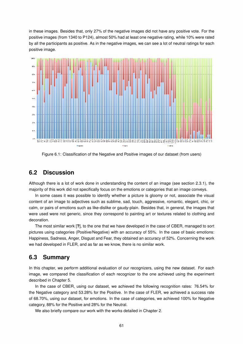
in these images. Besides that, only 27% of the negative images did not have any positive vote. For thepositive images (from 1340 to P124), almost 50% had at least one negative rating, while 10% were ratedby all the participants as positive. As in the negative images, we can see a lot of neutral ratings for eachpositive image.

Figure 6.1: Classification of the Negative and Positive images of our dataset (from users)

6.2 Discussion

Although there is a lot of work done in understanding the content of an image (see section 2.3.1), themajority of this work did not specifically focus on the emotions or categories that an image conveys.

In some cases it was possible to identify whether a picture is gloomy or not, associate the visualcontent of an image to adjectives such as sublime, sad, touch, aggressive, romantic, elegant, chic, orcalm, or pairs of emotions such as like-dislike or gaudy-plain. Besides that, in general, the images thatwere used were not generic, since they correspond to painting art or textures related to clothing anddecoration.

The most similar work [?], to the one that we have developed in the case of CBER, managed to sortpictures using categories (Positive/Negative) with an accuracy of 55%. In the case of basic emotions:Happiness, Sadness, Anger, Disgust and Fear, they obtained an accuracy of 52%. Concerning the workwe had developed in FLER, and as far as we know, there is no similar work.

6.3 Summary

In this chapter, we perform additional evaluation of our recognizers, using the new dataset. For eachimage, we compared the classification of each recognizer to the one achieved using the experimentdescribed in Chapter 5.

In the case of CBER, using our dataset, we achieved the following recognition rates: 76.54% forthe Negative category and 53.28% for the Positive. In the case of FLER, we achieved a success rateof 68.70%, using our dataset, for emotions. In the case of categories, we achieved 100% for Negativecategory, 88% for the Positive and 28% for the Neutral.

We also briefly compare our work with the works detailed in Chapter 2.

61

62

7Conclusions and Future Work

In this Chapter, we present a summary of the dissertation, our final conclusions and the contributions ofour work. We also present the new issues that might be addressed in the future.

7.1 Summary of the Dissertation

In this work, we proposed two solutions to identify the emotional content conveyed by an image, oneusing the Valence and Arousal values, and another using the content of the image, such as colors,texture or shape. We also provide a new dataset of images annotated with emotions, obtained fromexperiments with users.

In Chapter 2, we described the importance of emotions, as well as how they can be represented.Emotion in human cognition is essential and plays an important role in the daily life of human beings,namely in rational decision-making, perception, human interaction, and in human intelligence. Regardingthe emotion representation, there are two different perspectives: categorial and dimensional. Usually,the dimensional model is preferable because it could be used to locate discrete emotions in space, evenwhen no particular label could be used to define a certain feeling.

Along with it, we detailed the previous works in the recognition of emotions from images, and how im-age contents, such as faces, Color, Shape or Texture information, affect the way emotions are perceivedby the users. To describe how humans perceive and classify facial expressions of an emotion, there aretwo types of models: the continuous and categorical. The continuous model explains how expressionsof emotion can be seen at different intensities, whereas the categorical explains, among other findings,why the images in a morphing sequence between two emotions, like Happiness and Surprise, are per-ceived as either happy or surprise but not something in between. There have been developed modelsof the perception and classification of the six facial expressions of emotion. Initially, they used featureand Shape-based algorithms, but, in the last two decades, appearance-based models (AAM) have beenused.

We also described the relationship between emotions and the different visual characteristics of animage, namely Color, Shape, Texture, and Composition. Color is the most extensively used visualcontent for image retrieval since it is the basic constituent of images. Shape corresponds to an important

63

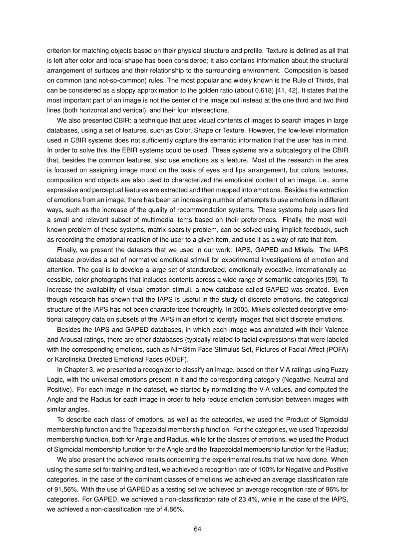
criterion for matching objects based on their physical structure and profile. Texture is defined as all thatis left after color and local shape has been considered; it also contains information about the structuralarrangement of surfaces and their relationship to the surrounding environment. Composition is basedon common (and not-so-common) rules. The most popular and widely known is the Rule of Thirds, thatcan be considered as a sloppy approximation to the golden ratio (about 0.618) [41, 42]. It states that themost important part of an image is not the center of the image but instead at the one third and two thirdlines (both horizontal and vertical), and their four intersections.

We also presented CBIR: a technique that uses visual contents of images to search images in largedatabases, using a set of features, such as Color, Shape or Texture. However, the low-level informationused in CBIR systems does not sufficiently capture the semantic information that the user has in mind.In order to solve this, the EBIR systems could be used. These systems are a subcategory of the CBIRthat, besides the common features, also use emotions as a feature. Most of the research in the areais focused on assigning image mood on the basis of eyes and lips arrangement, but colors, textures,composition and objects are also used to characterized the emotional content of an image, i.e., someexpressive and perceptual features are extracted and then mapped into emotions. Besides the extractionof emotions from an image, there has been an increasing number of attempts to use emotions in differentways, such as the increase of the quality of recommendation systems. These systems help users finda small and relevant subset of multimedia items based on their preferences. Finally, the most well-known problem of these systems, matrix-sparsity problem, can be solved using implicit feedback, suchas recording the emotional reaction of the user to a given item, and use it as a way of rate that item.

Finally, we present the datasets that we used in our work: IAPS, GAPED and Mikels. The IAPSdatabase provides a set of normative emotional stimuli for experimental investigations of emotion andattention. The goal is to develop a large set of standardized, emotionally-evocative, internationally ac-cessible, color photographs that includes contents across a wide range of semantic categories [59]. Toincrease the availability of visual emotion stimuli, a new database called GAPED was created. Eventhough research has shown that the IAPS is useful in the study of discrete emotions, the categoricalstructure of the IAPS has not been characterized thoroughly. In 2005, Mikels collected descriptive emo-tional category data on subsets of the IAPS in an effort to identify images that elicit discrete emotions.

Besides the IAPS and GAPED databases, in which each image was annotated with their Valenceand Arousal ratings, there are other databases (typically related to facial expressions) that were labeledwith the corresponding emotions, such as NimStim Face Stimulus Set, Pictures of Facial Affect (POFA)or Karolinska Directed Emotional Faces (KDEF).

In Chapter 3, we presented a recognizer to classify an image, based on their V-A ratings using FuzzyLogic, with the universal emotions present in it and the corresponding category (Negative, Neutral andPositive). For each image in the dataset, we started by normalizing the V-A values, and computed theAngle and the Radius for each image in order to help reduce emotion confusion between images withsimilar angles.

To describe each class of emotions, as well as the categories, we used the Product of Sigmoidalmembership function and the Trapezoidal membership function. For the categories, we used Trapezoidalmembership function, both for Angle and Radius, while for the classes of emotions, we used the Productof Sigmoidal membership function for the Angle and the Trapezoidal membership function for the Radius;

We also present the achieved results concerning the experimental results that we have done. Whenusing the same set for training and test, we achieved a recognition rate of 100% for Negative and Positivecategories. In the case of the dominant classes of emotions we achieved an average classification rateof 91,56%. With the use of GAPED as a testing set we achieved an average recognition rate of 96% forcategories. For GAPED, we achieved a non-classification rate of 23.4%, while in the case of the IAPS,we achieved a non-classification rate of 4.86%.

64

In chapter 4, we described a recognizer to classify an image with the corresponding emotion cate-gory: Positive or Negative, based on the content of the image, such as Color, Texture or Shape. Wealso presented the several studies that we have made, concerning the combinations of different visualfeatures, to select the best one for our recognizer. The recognizer uses a Vote classifier based on SMO,NB, LB, RF, and RSS, and is composed by CH, CM, NDC, and RCS features.

Finally, we presented the experimental results, in which, using a set of 156 images, for testing, thatwere not used for training, we achieved an average recognition rate of 72.44% (Negative: 87.18% andPositive: 57.69%).

In chapter 5, we described the experience performed to annotate a new dataset of images with theemotional content of each image, as well as the collected information about what users think about theexperience, and what influenced the way they felt during the visualization of an image. Next, we discussthe aspects that we considered as the most important: the way a person interprets an image, specificallythe context in which the image is inserted, the current emotional state of the person, and the previouspersonal experiences of the person.

We also presented the comparison about the agreement, for each image, between our dataset andMikels/GAPED datasets. In the case of the images from Mikels dataset, the agreement was 100% for allthe 4 Negative images, as well as for the only Positive image. The remaining two images were classifiedas Neutral by the people, although their original classification was Negative. For the GAPED dataset,we achieved 100% of agreement for the Negative category, and almost 90% for Positive. In the case ofthe Neutral category, only about 24% of the images were considerer as Neutral in both datasets, withthe majority, almost 77%, being considered Negative.

In chapter 6, we performed additional evaluation of our recognizers, using the new dataset. For eachimage, we compared the classification of each recognizer to the one achieved using the experimentdescribed in Chapter 5. We also briefly compare our work with the works detailed in Chapter 2.

In the case of CBER, using our dataset, we achieved the following recognition rates: 76.54% forthe Negative category and 53.28% for the Positive. In the case of FLER, we achieved a success rateof 68.70%, using our dataset, for emotions. In the case of categories, we achieved 100% for Negativecategory, 88% for the Positive and 28% for the Neutral.

7.2 Final Conclusions and Contributions

Although there is a lot of work regarding the retrieval of images based on their content, most of this workdid not take into account the emotions that an image conveys. Therefore, our work focused on retrievingthe emotions related to a given image, by providing two recognizers: one using the Valence and Arousalinformation from the image, and the other using the visual content of the image. This way, we increasedthe number of images annotated with their emotions without the need of manual classification, reducingboth the subjectivity of the classification and the extensive use of the same stimuli. In short, the maincontributions of this work were:

• A Fuzzy recognizer that achieved a recognition rate of 100% for categories of emotion and91.56% for emotions, using Mikels dataset [66]; for GAPED, the recognizer achieved an aver-age classification rate of 95.59% for the categories of emotion and, finally, using our dataset, itachieved a success rate of 68.70% for emotions, and, in the case of categories, it achieved 100%for Negative category, 88% for the Positive and 28% for the Neutral.

• A recognizer based on the content of the images, that has obtained a recognition rate of 87.18%for the Negative category and 57.69% for the Positive, using a dataset of images selected both

65

from IAPS and from GAPED datasets. Using our dataset, this recognizer achieved a recognitionrate of 76.54% for the Negative category and 53.28% for the Positive.

• A new dataset of 169 images from IAPS, Mikels and GAPED annotated with the dominant cate-gories and emotions, havin in account what users felt while viewing each image.

7.3 Future Work

From the experimental evaluation of the developed recognizers detailed in Section 3.2, 4.2 and Chapter6, we can establish new guidelines for the work to be done in the future.

Concerning FLER, we used 6 images for ADS, 11 for DS, 12 for F, 24 for DF, 31 for D, 43 for S,and finally, 114 for Ha, for the creation of each Fuzzy Set. As we can see, the distribution of the imagesaccording to each class of emotion is not balanced, and in the majority of the cases, there is a smallnumber of images of each. Given this, we consider important to use more annotated images to adjustthe Fuzzy Sets for each class of emotions, and consequently the Fuzzy Sets for each of the categories.

Considering the results obtained throughout this work in the case of the categories, the next possiblestep is to merge the two recognizers into one. If a particular image, provided as input to the “new”recognizer has information about their Valence and Arousal values, a weighting system should be usedbetween the values of DOM (assigned by FLER) and the estimated probability (assigned by the CBER)in order to classify the image. Otherwise, it should be used only CBER classification.

Further, we suggest to complement the new dataset with data collected using an BCI device (e.g.,Emotiv). This way, each image will have the emotion felt, and the emotion reported by the users. Anotherpossibility is to use the automatic identification of the category of emotions from content, in order toorganize or sort the results of an image search, or even to filter the images that will be displayed to theuser. Besides that, for example in therapy sessions, it may be helpful to use the emotional informationfrom the images and emotional state of the user, to improve their emotional state.

66

Bibliography

[1] D Aha and D Kibler. Instance-based learning algorithms. Machine Learning, 6:37–66, 1991.

[2] O AlZoubi, RA Calvo, and RH Stevens. Classification of eeg for affect recognition: an adaptive ap-proach. AI 2009: Advances in Artificial Intelligence Lecture Notes in Computer Science, 5866:52–61, 2009.

[3] JC Amante. Colorido : Identificacao da Cor Dominante de Fotografias. PhD thesis, 2011.

[4] JC Amante and MJ Fonseca. Fuzzy Color Space Segmentation to Identify the Same DominantColors as Users. DMS, 2012.

[5] Danny Oude Bos. EEG-based Emotion Recognition: The Influence of Visual and Auditory Stimuli.Capita Selecta Paper, 2007.

[6] Leo Breiman. Bagging predictors. Machine Learning, 24(2):123–140, 1996.

[7] Leo Breiman. Random Forests. Machine Learning, 45(1):5–32, 2001.

[8] Shih-Fu Chang, T Sikora, and A Purl. Overview of the MPEG-7 standard. Circuits and Systems forVideo Technology, IEEE Transactions on, 11(6):688–695, June 2001.

[9] SA Chatzichristofis and YS Boutalis. CEDD: color and edge directivity descriptor. A compact de-scriptor for image indexing and retrieval. Computer Vision Systems, pages 312–322, 2008.

[10] Savvas A Chatzichristofis, Y S Boutalis, and Mathias Lux. Selection of the proper compact compos-ite descriptor for improving content based image retrieval. In B Zagar, editor, Signal Processing,Pattern Recognition and Applications (SPPRA 2009), page 0, Calgary, Canada, February 2009.ACTA Press.

[11] Savvas A Chatzichristofis and Yiannis S Boutalis. FCTH: Fuzzy Color and Texture Histogram - ALow Level Feature for Accurate Image Retrieval. In Proceedings of the 2008 Ninth InternationalWorkshop on Image Analysis for Multimedia Interactive Services, WIAMIS ’08, pages 191–196,Washington, DC, USA, 2008. IEEE Computer Society.

[12] Chin-han Chen, MF Weng, SK Jeng, and YY Chuang. Emotion-based music visualization usingphotos. Advances in Multimedia Modeling, 4903:358–368, 2008.

[13] O da Pos and Paul Green-Armytage. Facial expressions, colours and basic emotions. Journal ofthe International Colour Association, 1:1–20, 2007.

[14] Elise S Dan-Glauser and Klaus R Scherer. The Geneva affective picture database (GAPED): a new730-picture database focusing on valence and normative significance. Behavior research methods,43(2):468–77, June 2011.

67

[15] Charles Darwin. The Expression of the Emotions in Man and Animals. 1872.

[16] Drago Datcu and L Rothkrantz.

[17] Ritendra Datta, Dhiraj Joshi, Jia Li, and James Z Wang. Studying Aesthetics in PhotographicImages Using a Computational Approach. In Proceedings of the 9th European Conference onComputer Vision - Volume Part III, ECCV’06, pages 288–301, Berlin, Heidelberg, 2006. Springer-Verlag.

[18] CM de Melo and Jonathan Gratch. Evolving expression of emotions through color in virtual hu-mans using genetic algorithms. Proceedings of the 1st International Conference on ComputationalCreativity ({ICCC-X)}, 2010.

[19] Peter Dunker, Stefanie Nowak, Andre Begau, and Cornelia Lanz. Content-based Mood Classi-fication for Photos and Music: A Generic Multi-modal Classification Framework and EvaluationApproach. In Proceedings of the 1st ACM International Conference on Multimedia InformationRetrieval, MIR ’08, pages 97–104, New York, NY, USA, 2008. ACM.

[20] Paul Ekman. Basic emotions, chapter 3, pages 45–60. John Wiley & Sons Ltd, New York, 1999.

[21] Paul Ekman and Wallace Friesen. Pictures of Facial Affect. Consulting Psychologists Press, PaloAlto, CA, 1976.

[22] Paul Ekman and Erika L. Rosenberg. What the Face Reveals: Basic and Applied Studies of Spon-taneous Expression Using the Facial Action Coding System (Facs) (Series in Affective Science).Oxford University Press, 2005.

[23] Elaine Fox. Emotion Science Cognitive and Neuroscientific Approaches to Understanding HumanEmotions, September 2008.

[24] J Friedman, T Hastie, and R Tibshirani. Additive Logistic Regression: a Statistical View of Boosting.Technical report, Stanford University, 1998.

[25] Syntyche Gbehounou, Francois Lecellier, Christine Fernandez-maloigne, and U M R Cnrs. Ex-traction of emotional impact in colour images. 6th European Conference on Colour in Graphics,Imaging and Vision, 2012.

[26] Franz Graf. JFeatureLib, 2012.

[27] Ramin Zabih Greg Pass. Comparing Images Using Joint Histograms. 1999.

[28] Mark Hall, Eibe Frank, and Geoffrey Holmes. The WEKA Data Mining Software: An Update. ACMSIGKDD, 11(1):10–18, 2009.

[29] Onur C Hamsici and Aleix M Martınez. Bayes Optimality in Linear Discriminant Analysis. IEEETrans. Pattern Anal. Mach. Intell., 30(4):647–657, 2008.

[30] Alan Hanjalic. Extracting Moods from Pictures and Sounds. IEEE SIGNAL PROCESSING MAGA-ZINE, (March 2006):90–100, 2006.

[31] R Haralick, K Shanmugam, and I Dinstein. Texture Features for Image Classification. IEEE Trans-actions on Systems, Man, and Cybernetics, 3(6), 1973.

[32] Lane Harrison, Drew Skau, and Steven Franconeri. Influencing visual judgment through affectivepriming. Proceedings of the SIGCHI Conference on Human Factors in Computing Systems, pages2949–2958, 2013.

68

[33] Trevor Hastie and Robert Tibshirani. Classification by Pairwise Coupling. In Michael I Jordan,Michael J Kearns, and Sara A Solla, editors, Advances in Neural Information Processing Systems,volume 10. MIT Press, 1998.

[34] Tin Kam Ho. The Random Subspace Method for Constructing Decision Forests. IEEE Transactionson Pattern Analysis and Machine Intelligence, 20(8):832–844, 1998.

[35] D.H. Hockenbury and S.E. Hockenbury. Discovering psychology. New York: Worth Publishers,2007.

[36] Jing Huang, S Ravi Kumar, Mandar Mitra, Wei-Jing Zhu, and Ramin Zabih. Image Indexing UsingColor Correlograms. 1997 IEEE Conference on Computer Vision and Pattern Recognition, 0:762,1997.

[37] George H John and Pat Langley. Estimating Continuous Distributions in Bayesian Classifiers. InEleventh Conference on Uncertainty in Artificial Intelligence, pages 338–345, San Mateo, 1995.Morgan Kaufmann.

[38] Evi Joosten, GV Lankveld, and Pieter Spronck. Colors and emotions in video games. 11th Inter-national Conference on Entertainment Computing, 2010.

[39] Dhiraj Joshi, Ritendra Datta, Elena Fedorovskaya, Quang-tuan Luong, James Z Wang, Li Jia, andJiebo Luo. Aesthetics and Emotions in Images [A computational perspective ]. IEEE Signal Pro-cessing Magazine, (SEPTEMBER 2011):94–115, 2011.

[40] Takeo Kanade. Picture Processing System by Computer Complex and Recognition of HumanFaces. 1973.

[41] S S Keerthi, S K Shevade, C Bhattacharyya, and K R K Murthy. Improvements to Platt’s SMOAlgorithm for SVM Classifier Design. Neural Computation, 13(3):637–649, 2001.

[42] A Khokher and R Talwar. Content-based image retrieval: state of the art and challenges. (IJAEST)INTERNATIONAL JOURNAL OF ADVANCED ENGINEERING SCIENCES AND TECHNOLOGIES,9(2):207–211, 2011.

[43] Youngrae Kim, So-jung Kim, and Eun Yi Kim. EBIR: Emotion-based image retrieval. 2009 Digestof Technical Papers International Conference on Consumer Electronics, pages 1–2, January 2009.

[44] J Kittler, M Hatef, Robert P W Duin, and J Matas. On combining classifiers. IEEE Transactions onPattern Analysis and Machine Intelligence, 20(3):226–239, 1998.

[45] Hans-Peter Kriegel, Erich Schubert, and Arthur Zimek. Evaluation of Multiple Clustering Solutions.In MultiClust@ECML/PKDD, pages 55–66, 2011.

[46] Kai Kuikkaniemi, Toni Laitinen, Marko Turpeinen, Timo Saari, Ilkka Kosunen, and Niklas Ravaja.The influence of implicit and explicit biofeedback in first-person shooter games. CHI’10 Proceedingsof the SIGCHI Conference on Human Factors in Computing Systems, pages 859–868, 2010.

[47] Ludmila I Kuncheva. Combining Pattern Classifiers: Methods and Algorithms. John Wiley andSons, Inc., 2004.

[48] R D Lane, E M Reiman, G L Ahern, G E Schwartz, and R J Davidson. Neuroanatomical correlatesof happiness, sadness, and disgust. The American journal of psychiatry, 154(7):926–33, July 1997.

69

[49] P J Lang. The emotion probe: Studies of motivation and attention. American psychologist, 50:372,1995.

[50] P.J. Lang, M.M. Bradley, and B.N. Cuthbert. International affective picture system (IAPS): Affectiveratings of pictures and instruction manual. NIMH Center for the Study of Emotion and Attention,1997.

[51] Christine L. Larson, Joel Aronoff, and Elizabeth L. Steuer. Simple geometric shapes are implicitlyassociated with affective value. Motivation and Emotion, 36(3):404–413, October 2011.

[52] S le Cessie and J C van Houwelingen. Ridge Estimators in Logistic Regression. Applied Statistics,41(1):191–201, 1992.

[53] T M C Lee, H-L Liu, C C H Chan, S-Y Fang, and J-H Gao. Neural activities associated with emotionrecognition observed in men and women. Molecular psychiatry, 10(5):450–5, May 2005.

[54] Yisi Liu, Olga Sourina, and MK Nguyen. Real-time EEG-based emotion recognition and its appli-cations. Transactions on computational science XII, 2011.

[55] David G. Lowe. Three-dimensional object recognition from single two-dimensional images. ArtificialIntelligence, 31:355–395, 1987.

[56] Xin Lu, Poonam Suryanarayan, Reginald B Adams, Jia Li, Michelle G Newman, and James Z Wang.On Shape and the Computability of Emotions. Proceedings of the ACM Multimedia Conference,2012.

[57] Marcel P. Lucassen, Theo Gevers, and Arjan Gijsenij. Texture affects color emotion. Color Research& Application, 36(6):426–436, December 2011.

[58] Mathias Lux and Savvas A Chatzichristofis. Lire: Lucene Image Retrieval: An Extensible JavaCBIR Library. In Proceedings of the 16th ACM International Conference on Multimedia, MM ’08,pages 1085–1088, New York, NY, USA, 2008. ACM.

[59] Mathias Lux and Oge Marques. Visual Information Retrieval Using Java and LIRE. SynthesisLectures on Information Concepts, Retrieval, and Services. Morgan & Claypool Publishers, 2013.

[60] Jana Machajdik and Allan Hanbury. Affective image classification using features inspired by psy-chology and art theory. Proceedings of the international conference on Multimedia - MM ’10,page 83, 2010.

[61] D Marr. Early processing of visual information. Philosophical Transactions of the Royal Society ofLondon, B275:483–524, 1976.

[62] Christian Martin, Uwe Werner, and HM Gross. A real-time facial expression recognitionsystem based on active appearance models using gray images and edge images. IEEE,216487(216487):1–6, 2008.

[63] Aleix Martinez and Shichuan Du. A Model of the Perception of Facial Expressions of Emotion byHumans: Research Overview and Perspectives. Journal of Machine Learning Research : JMLR,13:1589–1608, May 2012.

[64] S Marcelja. Mathematical description of the responses of simple cortical cells. J. Opt. Soc. Am.,70(11):1297–1300, November 1980.

70

[65] Celso De Melo and Ana Paiva. Expression of emotions in virtual humans using lights, shadows,composition and filters. Affective Computing and Intelligent Interaction, pages 549–560, 2007.

[66] Joseph a Mikels, Barbara L Fredrickson, Gregory R Larkin, Casey M Lindberg, Sam J Maglio,and Patricia a Reuter-Lorenz. Emotional category data on images from the International AffectivePicture System. Behavior research methods, 37(4):626–30, November 2005.

[67] Katarzyna Agnieszka Olkiewicz and Urszula Markowska-kaczmar. Emotion-based image retrieval- An artificial neural network approach. Proceedings of the International Multiconference on Com-puter Science and Information Technology, pages 89–96, 2010.

[68] Michael Jones Paul Viola. Robust Real-time Object Detection. International Journal of ComputerVision, 2001.

[69] W.R. Picard. Affective Computing, 1995.

[70] J Platt. Fast Training of Support Vector Machines using Sequential Minimal Optimization. InB Schoelkopf, C Burges, and A Smola, editors, Advances in Kernel Methods - Support VectorLearning. MIT Press, 1998.

[71] R. Plutchik. The nature of Emotions. Am. Sci., 89(4):344–350, 2001.

[72] Jonathan Posner, James a Russell, and Bradley S Peterson. The circumplex model of affect:an integrative approach to affective neuroscience, cognitive development, and psychopathology.Development and psychopathology, 17(3):715–34, January 2005.

[73] Ross Quinlan. C4.5: Programs for Machine Learning. Morgan Kaufmann Publishers, San Mateo,CA, 1993.

[74] Thomas Rorissa, Abebe; Clough, Paul; Deselaers. Exploring the Relationship Between Feature.JOURNAL OF THE AMERICAN SOCIETY FOR INFORMATION SCIENCE AND TECHNOLOGY,59(5):770–784, 2008.

[75] J A Russell. A circumplex model of affect. Journal of personality and social psychology, 39(6):1161–1178, 1980.

[76] Stefanie Schmidt and WG Stock. Collective indexing of emotions in images. A study in emotionalinformation retrieval. JOURNAL OF THE AMERICAN SOCIETY FOR INFORMATION SCIENCEAND TECHNOLOGY, 60(February):863–876, 2009.

[77] SG Shaila and A Vadivel. Content-Based Image Retrieval Using Modified Human Colour PerceptionHistogram. ITCS, SIP, JSE-2012, CS & IT, pages 229–237, 2012.

[78] DS Shete and MS Chavan. Content Based Image Retrieval: Review. International Journal ofEmerging Technology and Advanced Enginnering, 2(9):85–90, 2012.

[79] A. Smith. A new set of norms. Behavior Research Methods, Instruments, and Computers, (3x(x),xxx-xxx), 2004.

[80] A. Smith. Smith2004norms.txt. Retrieved October 2, 2004 from Psychonomic Society WebArchieve: http://www.psychonomic.org/ARCHIEVE/, 2004.

[81] Martin Solli. Color Emotions in Large Scale Content Based Image Indexing. PhD thesis, 2011.

[82] H Tamura, S Mori, and T Yamawaki. Texture features corresponding to visual perception. IEEETransactions on Systems, Man and Cybernetics, 8(6), 1978.

71

[83] M Tkalcic, A Kosir, and J Tasic. Affective recommender systems: the role of emotions in recom-mender systems. Decisions@RecSys, 2011.

[84] Marko Tkalcic, Urban Burnik, and Andrej Kosir. Using affective parameters in a content-basedrecommender system for images. User Modeling and User-Adapted Interaction, 20(4):279–311,September 2010.

[85] Koen E a van de Sande, Theo Gevers, and Cees G M Snoek. Evaluating color descriptors forobject and scene recognition. IEEE transactions on pattern analysis and machine intelligence,32(9):1582–96, September 2010.

[86] Paul Viola and Michael Jones. Rapid object detection using a boosted cascade of simple features.In Computer Vision and Pattern Recognition, 2001. CVPR 2001. Proceedings of the 2001 IEEEComputer Society Conference on, volume 1, pages I—-511. IEEE, 2001.

[87] WN Wang and YL Yu. Image emotional semantic query based on color semantic descrip-tion. Proceedings of the Fourth International Conference on Machine Learning and Cybernetics,Guangzhou, (August):18–21, 2005.

[88] X Wang, Jia Jia, Yongxin Wang, and Lianhong Cai. Modeling the Relationship Between Texture Se-mantics and Textile Images. Research Journal of Applied Sciences, Engineering and Technology,3(9):977–985, 2011.

[89] HW Yoo. Visual-based emotional descriptor and feedback mechanism for image retrieval. Journalof information science and engineering, 1227:1205–1227, 2006.

[90] L. A. Zadeh. Fuzzy Sets*. Information and Control, 8:338–353, 1965.

72

Appendix A

% NB RF Log J48 SMO Ibk Bag RSS LBACC 56.78 56.78 50.00 57.20 55.93 56.36 60.17 58.90 58.47CH 61.44 56.36 61.44 56.36 65.25 58.05 59.75 60.59 61.86CM 53.81 52.12 56.78 48.73 52.97 47.03 51.27 52.54 55.51NDC 50.00 51.27 50.85 52.12 52.12 51.69 47.03 51.69 52.54OH 58.05 56.78 53.81 53.39 58.90 49.58 41.27 52.97 54.66PCFH 65.68 57.63 61.86 55.93 63.98 55.80 56.78 60.59 57.63PCFHS 66.53 54.66 50.85 56.36 58.90 54.66 60.59 58.90 57.20RCS 57.20 58.05 61.02 57.63 58.05 54.24 62.29 60.17 61.02RT 56.78 61.02 56.78 60.17 61.86 61.44 59.32 58.90 61.02EH 46.18 52.54 47.03 55.51 44.92 49.58 48.73 47.46 46.19Gabor 47.88 45.76 36.86 50.00 50.85 45.34 43.22 43.64 43.22Haralick 49.58 53.81 56.78 48.31 55.51 46.19 50.42 54.24 50.42Tamura 51.69 50.00 55.93 47.03 52.97 52.54 47.88 46.19 47.88CEDD 62.71 61.44 55.08 55.08 58.90 54.66 62.29 60.59 58.05FCTH 51.69 53.81 51.27 52.12 55.93 52.97 55.93 55.08 58.05JCD 62.29 59.75 52.54 59.32 58.90 53.81 58.47 59.32 59.32Average 56.14 55.11 53.68 54.08 56.62 52.75 54.09 55.11 55.19

Table A1: Simple and Meta classifiers results for each feature

% V1 V2 V3 V4 V5 V6ACC 55.93 56.78 59.32 56.78 53.39 56.36CH 65.68 63.56 63.98 63.14 63.56 64.83CM 52.54 51.27 51.69 52.97 52.97 52.97NDC 52.97 52.54 51.69 52.12 52.12 52.12OH 57.63 58.05 59.75 59.75 58.47 58.90PCFH 64.41 61.86 64.83 64.83 65.68 63.98PCFHS 59.75 63.14 62.71 62.29 60.17 58.90RCS 61.02 60.17 60.17 59.75 60.59 58.05RT 64.41 64.83 63.98 61.86 61.44 61.86EH 44.07 44.92 44.92 44.92 44.92 44.92Gabor 44.07 44.07 45.76 48.73 46.19 51.27Haralick 57.20 56.78 55.93 56.36 54.66 55.51Tamura 56.36 53.81 52.54 53.81 52.97 52.97CEDD 60.59 62.71 61.02 61.86 58.47 58.90FCTH 60.17 59.75 62.71 61.44 59.75 56.78JCD 58.90 63.56 62.29 63.56 59.75 58.90Average 57.23 57.36 57.71 57.76 56.57 56.70

Table A2: Vote classifiers results for each feature

% V1 V2 V3 V4 V5 V6ACC 55.93 56.78 59.32 56.78 53.39 56.36CH 65.68 63.56 63.98 63.14 63.56 64.83CM 52.54 51.27 51.69 52.97 52.97 52.97

73

NDC 52.97 52.54 51.69 52.12 52.12 52.12OH 57.63 58.05 59.75 59.75 58.47 58.90PFCH 64.41 61.86 64.83 64.83 65.68 63.98PFCHS 59.75 63.14 62.71 62.29 60.17 58.90RCS 61.02 60.17 60.17 59.75 60.59 58.05Average 58.74 58.42 59.27 58.95 58.37 58.26

Table A3: Results for Color using one feature

% V1 V2 V3 V4 V5 V6ACC+CH 56.36 59.32 56.36 58.90 54.66 58.05ACC+CM 55.51 55.93 57.78 55.08 52.97 56.36ACC+NDC 54.66 58.05 58.47 56.78 53.81 56.36ACC+OH 56.36 61.02 57.20 57.20 53.81 57.63ACC+PFCH 55.93 57.20 56.78 54.24 55.51 57.20ACC+PFCHS 53.39 56.36 56.78 56.36 51.69 56.78ACC+RCS 55.08 59.32 58.05 56.36 53.39 57.20CH+CM 65.68 65.25 63.56 61.86 62.71 64.41CH+NDC 66.95 64.83 62.29 63.56 63.98 65.25CH+OH 66.95 64.83 64.41 63.98 65.25 66.52CH+PFCH 64.83 63.98 64.41 63.98 63.56 65.25CH+PFCHS 63.98 64.41 63.14 64.83 60.59 58.90CH+RCS 65.25 68.22 64.83 64.83 66.10 67.80CM+NDC 48.73 51.27 49.58 53.81 52.54 52.54CM+OH 58.05 58.47 58.47 59.32 60.17 59.32CM+PFCH 62.29 60.17 61.86 62.71 62.29 61.86CM+PFCHS 61.02 63.14 63.14 63.56 61.02 58.90CM+RCS 61.02 61.02 60.59 58.90 59.32 56.78NDC+OH 57.20 58.32 59.75 59.32 58.47 58.90NDC+PFCH 64.83 63.56 65.25 65.68 66.10 64.41NDC+PFCHS 61.44 62.29 63.56 62.71 60.59 59.75NDC+RCS 63.14 60.59 60.59 59.75 59.32 58.47OH+PFCH 62.29 62.29 62.71 62.71 62.71 61.44OH+PFCHS 67.37 62.72 64.83 64.83 64.83 61.44OH+RCS 62.29 60.59 61.86 62.29 61.44 61.02PFCH+PFCHS 61.02 63.14 63.14 62.29 59.32 60.59PFCH+RCS 63.98 63.56 65.25 65.68 63.98 65.68PFCHS+RCS 64.41 64.83 65.68 66.95 63.14 61.44Average 60.71 61.24 61.08 61.02 59.76 60.37

Table A4: Results for combination of two Color features

% V1 V2 V3 V4 V5 V6ACC+CH+CM 57.20 59.75 58.47 59.32 54.24 57.63ACC+CH+NDC 56.36 58.47 58.47 59.32 54.24 58.05ACC+CH+OH 54.66 57.20 55.51 56.36 55.08 57.20ACC+CH+PFCH 56.36 57.63 55.93 57.20 53.39 57.63ACC+CH+PFCHS 57.63 58.05 56.36 56.36 54.66 58.90ACC+CH+RCS 57.20 59.32 60.59 60.17 53.39 58.05ACC+CM+NDC 54.66 55.93 57.63 55.08 50.85 56.78ACC+CM+OH 52.54 56.36 55.51 54.66 51.27 57.20ACC+CM+PFCH 53.81 56.78 56.78 55.51 54.24 57.63ACC+CM+PFCHS 54.66 58.05 57.20 56.36 52.12 58.05ACC+CM+RCS 55.08 58.48 56.78 55.93 52.12 57.20ACC+NDC+OH 56.78 56.78 57.78 57.63 54.24 57.63ACC+NDC+PFCH 56.78 57.20 55.93 54.66 55.08 57.63ACC+NDC+PFCHS 52.96 56.36 56.78 56.36 52.54 57.20ACC+NDC+RCS 58.90 60.17 58.90 57.20 56.78 57.63ACC+OH+PFCH 59.32 57.63 58.05 55.93 58.47 58.05

74

ACC+OH+PFCHS 53.39 58.90 57.63 56.36 53.39 55.93ACC+OH+RCS 57.20 60.17 58.90 57.20 56.36 57.63ACC+PFCH+PFCHS 57.20 58.90 57.20 57.63 53.39 56.36ACC+PFCH+RCS 55.51 60.59 59.32 58.48 53.39 56.78ACC+PFCHS+RCS 54.66 58.90 57.20 57.20 53.82 57.63CH+CM+NDC 64.41 65.25 63.56 62.72 63.56 65.25CH+CM+OH 66.10 66.52 62.29 62.70 63.25 64.83CH+CM+PFCH 64.83 63.98 63.14 64.41 63.14 64.41CH+CM+PFCHS 63.56 63.98 63.98 64.83 61.02 58.90CH+CM+RCS 63.98 67.80 63.56 65.25 65.25 66.95CH+NDC+OH 66.52 65.25 62.71 63.56 63.68 66.25CH+NDC+PFCH 64.41 63.14 63.14 64.41 63.98 66.10CH+NDC+PFCHS 63.98 63.56 63.98 65.68 62.29 58.90CH+NDC+RCS 66.95 67.37 65.69 65.68 66.10 67.80CH+OH+PFCH 65.68 64.41 61.86 63.14 63.56 64.41CH+OH+PFCHS 64.83 65.68 64.83 66.10 63.14 59.32CH+OH+RCS 69.50 68.64 65.25 66.53 69.07 67.80CH+PFCH+PFCHS 61.86 63.98 62.29 63.98 58.05 61.44CH+PFCH+RCS 66.52 66.52 66.52 66.52 64.83 65.68CH+PFCHS+RCS 64.83 64.83 65.25 64.41 61.86 61.44CM+NDC+OH 58.90 58.90 59.75 59.32 60.17 59.32CM+NDC+PFCH 63.56 63.14 63.98 63.56 63.14 63.14CM+NDC+PFCHS 61.86 60.17 63.56 63.56 61.02 58.90CM+NDC+RCS 61.44 60.59 59.32 59.32 59.32 55.51CM+OH+PFCH 61.02 61.44 60.59 60.59 61.86 61.02CM+OH+PFCHS 63.56 63.14 63.98 63.56 62.71 58.90CM+OH+RCS 60.59 60.59 61.86 62.29 60.59 60.17CM+PFCH+PFCHS 61.86 63.14 63.98 62.71 60.59 60.17CM+PFCH+RCS 62.29 62.29 63.98 63.56 62.71 62.71CM+PFCHS+RCS 62.71 61.44 61.44 63.98 60.59 58.05NDC+OH+PFCH 62.29 61.02 62.29 63.14 62.71 61.86NDC+OH+PFCHS 64.83 64.83 64.83 64.41 63.98 61.02NDC+OH+RCS 60.59 58.48 61.86 61.85 61.02 60.59NDC+PFCH+PFCHS 61.44 64.41 61.86 61.86 60.59 60.59NDC+PFCH+RCS 63.14 62.29 64.41 64.83 65.25 64.83NDC+PFCHS+RCS 63.98 65.68 64.83 67.37 62.29 62.72OH+PFCH+PFCHS 63.98 63.56 62.29 62.29 62.71 58.05OH+PFCH+RCS 61.44 63.14 65.25 64.83 62.29 63.98OH+PFCHS+RCS 64.83 67.37 66.95 66.10 64.83 60.59PFCH+PFCHS+RCS 61.86 66.10 66.52 66.52 60.17 60.59Average 60.66 61.68 61.22 61.26 59.36 60.34

Table A5: Results for combination of three Color features

% V1 V2 V3 V4 V5 V6ACC+CH+CM+NDC 56.36 58.05 59.75 58.90 53.81 57.63ACC+CH+CM+OH 56.78 59.32 59.32 57.20 55.08 58.48ACC+CH+CM+PFCH 55.51 58.05 59.32 58.90 52.97 57.20ACC+CH+CM+PFCHS 58.05 57.63 59.75 56.36 55.93 59.75ACC+CH+CM+RCS 56.78 59.32 59.32 59.75 53.81 57.20ACC+CM+NDC+OH 54.66 55.93 57.63 55.08 50.85 56.78ACC+CM+NDC+PFCH 56.36 58.05 56.78 55.51 53.81 57.63ACC+CM+NDC+PFCHS 56.78 56.78 54.24 56.78 50.85 58.05ACC+CM+NDC+RCS 56.36 60.17 60.17 56.78 54.66 58.05ACC+NDC+OH+PFCH 58.05 58.05 57.20 55.08 57.20 58.05ACC+NDC+OH+PFCHS 56.78 56.78 56.78 57.63 54.24 57.63ACC+NDC+OH+RCS 55.93 59.75 58.47 57.20 57.20 58.05ACC+OH+PFCH+PFCHS 55.93 58.90 57.63 56.78 53.81 56.36ACC+OH+PFCH+RCS 55.93 60.17 59.32 59.32 55.93 57.20ACC+PFCH+PFCHS+RCS 59.32 59.32 57.63 58.47 54.66 57.63

75

CH+CM+NDC+OH 66.10 64.41 60.59 62.71 65.25 64.83CH+CM+NDC+PFCH 63.98 64.83 65.25 64.83 63.56 64.41CH+CM+NDC+PFCHS 63.98 63.14 62.29 65.68 61.44 57.20CH+CM+NDC+RCS 66.10 68.64 65.25 66.10 65.68 67.80CM+NDC+OH+PFCH 62.29 61.44 62.71 62.29 63.56 62.29CM+NDC+OH+PFCHS 63.56 62.71 62.71 63.56 63.56 59.75CM+NDC+OH+RCS 61.44 60.59 62.71 61.86 60.59 59.75NDC+OH+PFCH+PFCHS 62.29 63.98 61.44 62.29 61.44 58.05NDC+OH+PFCH+RCS 63.98 63.14 63.98 64.83 62.71 62.71NDC+OH+PCFHS+RCS 66.10 65.78 65.68 66.10 65.68 60.59NDC+PFCH+PFCHS+RCS 61.02 63.14 65.25 65.68 58.90 60.17OH+PFCH+PFCHS+RCS 65.25 61.02 63.98 63.56 62.29 60.17Average 59.84 60.71 60.56 60.34 58.13 59.39

Table A6: Results for combination of four Color features

% V1 V2 V3 V4 V5 V6ACC+CH+CM+NDC+OH 57.63 58.90 57.63 56.36 55.93 58.48ACC+CH+CM+NDC+PFCH 57.20 59.75 59.75 59.32 53.81 58.05ACC+CH+CM+NDC+PFCHS 58.90 58.05 59.75 56.26 55.51 59.76ACC+CH+CM+NDC+RCS 58.90 61.44 60.59 59.75 55.08 57.63ACC+CM+NDC+OH+PFCH 57.63 58.05 57.2 56.78 56.36 58.05ACC+CM+NDC+OH+PFCHS 56.78 58.05 58.9 55.93 54.66 57.63ACC+CM+NDC+OH+RCS 56.36 60.17 58.47 56.78 54.66 58.05ACC+NDC+OH+PFCH+PFCHS 55.51 57.63 58.47 56.35 54.24 57.63ACC+NDC+OH+PFCH+RCS 58.47 59.32 59.75 59.32 57.63 57.20ACC+OH+PFCH+PFCHS+RCS 57.20 58.90 59.75 58.05 54.66 57.20CH+CM+NDC+OH+PFCH 65.25 62.71 63.56 64.41 63.56 64.41CH+CM+NDC+OH+PFCHS 65.25 64.41 64.83 66.95 62.71 58.90CH+CM+NDC+OH+RCS 65.25 67.80 62.71 63.98 64.41 65.25CM+NDC+OH+PFCH+PFCHS 61.86 61.44 61.02 62.71 59.75 58.47CM+NDC+OH+PFCH+RCS 62.71 61.44 62.71 63.14 62.28 61.44NDC+OH+PFCH+PFCHS+RCS 65.68 63.14 64.41 63.98 63.14 60.17Average 60.04 60.70 60.59 60.00 58.02 59.27

Table A7: Results for combination of five Color features

% V1 V2 V3 V4 V5 V6ACC+CH+CM+NDC+OH+PFCH 56.78 61.44 59.75 58.05 56.36 58.47ACC+CH+CM+NDC+OH+PFCHS 57.63 60.59 58.90 56.78 55.51 58.90ACC+CH+CM+NDC+OH+RCS 58.47 58.47 58.47 58.90 55.93 58.05ACC+CH+CM+NDC+PFCH+PFCHS 59.75 60.17 60.59 57.20 54.66 59.32ACC+CH+CM+NDC+PFCH+RCS 58.05 60.59 60.17 59.74 55.93 57.20ACC+CH+CM+NDC+PFCHS+RCS 58.90 59.32 60.17 59.75 55.51 58.90ACC+CH+CM+OH+PFCH+PFCHS 61.44 59.75 57.20 56.78 56.34 58.90ACC+CH+CM+OH+PFCH+RCS 58.47 58.90 59.75 60.17 57.63 57.20ACC+CH+CM+OH+PFCHS+RCS 59.32 60.59 59.75 60.17 55.93 58.05ACC+CM+NDC+OH+PFCH+PFCHS 56.78 58.90 58.47 55.93 53.81 58.05ACC+CM+NDC+OH+PFCH+RCS 57.20 58.90 58.05 59.32 57.35 58.05ACC+CM+NDC+OH+PFCHS+RCS 57.63 60.59 60.59 59.32 54.66 58.90ACC+NDC+OH+PFCH+PFCHS+RCS 57.20 59.75 58.47 58.05 53.81 57.20CH+CM+NDC+OH+PFCH+PFCHS 63.56 63.14 66.10 67.38 61.86 61.02CH+CM+NDC+OH+PFCH+RCS 65.68 67.80 65.25 64.83 63.14 64.41CH+CM+NDC+OH+PFCHS+RCS 63.98 64.83 64.83 65.25 63.14 61.86CM+NDC+OH+PFCH+PFCHS+RCS 63.56 64.41 63.56 62.29 61.44 59.75Average 59.67 61.07 60.59 59.99 57.24 59.07

Table A8: Results for combination of six Color features

76

% V1 V2 V3 V4 V5 V6ACC+CH+CM+NDC+OH+PFCH+PFCHS 59.75 60.17 60.59 57.20 54.66 59.32ACC+CH+CM+NDC+OH+PFCH+RCS 58.47 61.86 58.90 60.17 56.36 57.63ACC+CH+CM+NDC+OH+PFCHS+RCS 58.48 61.86 62.71 59.75 56.36 58.90ACC+CH+CM+NDC+PFCH+PFCHS+RCS 58.90 60.59 61.02 59.32 55.08 60.17ACC+CH+CM+OH+PFCH+PFCHS+RCS 62.29 61.44 59.32 58.90 58.05 60.59ACC+CH+NDC+OH+PFCH+PFCHS+RCS 59.32 61.44 60.17 58.90 55.51 58.90ACC+CM+NDC+OH+PFCH+PFCHS+RCS 57.63 60.59 58.9 58.90 54.66 59.32CH+CM+NDC+OH+PFCH+PFCHS+RCS 65.68 63.98 66.95 65.68 62.71 63.14Average 60.07 61.49 61.07 59.85 56.67 59.75

Table A9: Results for combination of seven Color features

% V1 V2 V3 V4 V5 V6ALL 60.59 59.75 59.32 58.90 56.36 60.59

Table A10: Results for combination of all Color features

% V1 V2 V3 V4 V5 V6CH 65.68 63.56 63.98 63.14 63.56 64.83OH 57.63 58.05 59.75 59.75 58.47 58.90PFCH 64.41 61.86 64.83 64.83 65.68 63.98PFCHS 59.75 63.14 62.71 62.29 60.17 58.90RCS 61.02 60.17 60.17 59.75 60.59 58.05CH+CM 65.68 65.25 63.56 61.86 62.71 64.41CH+NDC 66.95 64.83 62.29 63.56 63.98 65.25CH+OH 66.95 64.83 64.41 63.98 65.25 66.52CH+PFCH 64.83 63.98 64.41 63.98 63.56 65.25CH+PFCHS 63.98 64.41 63.14 64.83 60.59 58.90CH+RCS 65.25 68.22 64.83 64.83 66.10 67.80CM+PFCH 62.29 60.17 61.86 62.71 62.29 61.86CM+PFCHS 61.02 63.14 63.14 63.56 61.02 58.90NDC+PFCH 64.83 63.56 65.25 65.68 66.10 64.41NDC+PFCHS 61.44 62.29 63.56 62.71 60.59 59.75OH+PFCH 62.29 62.29 62.71 62.71 62.71 61.44OH+PFCHS 67.37 62.72 64.83 64.83 64.83 61.44OH+RCS 62.29 60.59 61.86 62.29 61.44 61.02PFCH+PFCHS 61.02 63.14 63.14 62.29 59.32 60.59PFCH+RCS 63.98 63.56 65.25 65.68 63.98 65.68PFCHS+RCS 64.41 64.83 65.68 66.95 63.14 61.44CH+CM+NDC 64.41 65.25 63.56 62.72 63.56 65.25CH+CM+OH 66.10 66.52 62.29 62.70 63.25 64.83CH+CM+PFCH 64.83 63.98 63.14 64.41 63.14 64.41CH+CM+PFCHS 63.56 63.98 63.98 64.83 61.02 58.90CH+CM+RCS 63.98 67.80 63.56 65.25 65.25 66.95CH+NDC+OH 66.52 65.25 62.71 63.56 63.68 66.25CH+NDC+PFCH 64.41 63.14 63.14 64.41 63.98 66.10CH+NDC+PFCHS 63.98 63.56 63.98 65.68 62.29 58.90CH+NDC+RCS 66.95 67.37 65.69 65.68 66.1 67.8CH+OH+PFCH 65.68 64.41 61.86 63.14 63.56 64.41CH+OH+PFCHS 64.83 65.68 64.83 66.1 63.14 59.32CH+OH+RCS 69.50 68.64 65.25 66.53 69.07 67.80CH+PFCH+PFCHS 61.86 63.98 62.29 63.98 58.05 61.44CH+PFCH+RCS 66.52 66.52 66.52 66.52 64.83 65.68CH+PFCHS+RCS 64.83 64.83 65.25 64.41 61.86 61.44CM+NDC+PFCH 63.56 63.14 63.98 63.56 63.14 63.14CM+NDC+PFCHS 61.86 60.17 63.56 63.56 61.02 58.90CM+OH+PFCHS 63.56 63.14 63.98 63.56 62.71 58.90CM+PFCH+PFCHS 61.86 63.14 63.98 62.71 60.59 60.17

77

CM+PFCH+RCS 62.29 62.29 63.98 63.56 62.71 62.71CM+PFCHS+RCS 62.71 61.44 61.44 63.98 60.59 58.05NDC+OH+PFCH 62.29 61.02 62.29 63.14 62.71 61.86NDC+OH+PFCHS 64.83 64.83 64.83 64.41 63.98 61.02NDC+OH+RCS 60.59 58.48 61.86 61.85 61.02 60.59NDC+PFCH+PFCHS 61.44 64.41 61.86 61.86 60.59 60.59NDC+PFCH+RCS 63.14 62.29 64.41 64.83 65.25 64.83NDC+PFCHS+RCS 63.98 65.68 64.83 67.37 62.29 62.72OH+PFCH+PFCHS 63.98 63.56 62.29 62.29 62.71 58.05OH+PFCH+RCS 61.44 63.14 65.25 64.83 62.29 63.98OH+PFCHS+RCS 64.83 67.37 66.95 66.10 64.83 60.59PFCH+PFCHS+RCS 61.86 66.10 66.52 66.52 60.17 60.59CH+CM+NDC+OH 66.10 64.41 60.59 62.71 65.25 64.83CH+CM+NDC+PFCH 63.98 64.83 65.25 64.83 63.56 64.41CH+CM+NDC+PFCHS 63.98 63.14 62.29 65.68 61.44 57.20CH+CM+NDC+RCS 66.10 68.64 65.25 66.10 65.68 67.80CM+NDC+OH+PFCH 62.29 61.44 62.71 62.29 63.56 62.29CM+NDC+OH+PFCHS 63.56 62.71 62.71 63.56 63.56 59.75CM+NDC+OH+RCS 61.44 60.59 62.71 61.86 60.59 59.75NDC+OH+PFCH+PFCHS 62.29 63.98 61.44 62.29 61.44 58.05NDC+OH+PFCH+RCS 63.98 63.14 63.98 64.83 62.71 62.71OH+PFCH+PFCHS+RCS 65.25 61.02 63.98 63.56 62.29 60.17CH+CM+NDC+OH+PFCH 65.25 62.71 63.56 64.41 63.56 64.41CH+CM+NDC+OH+PFCHS 65.25 64.41 64.83 66.95 62.71 58.9CH+CM+NDC+OH+RCS 65.25 67.8 62.71 63.98 64.41 65.25CM+NDC+OH+PFCH+PFCHS 61.86 61.44 61.02 62.71 59.75 58.47CM+NDC+OH+PFCH+RCS 62.71 61.44 62.71 63.14 62.28 61.44NDC+OH+PFCH+PFCHS+RCS 65.68 63.14 64.41 63.98 63.14 60.17CH+CM+NDC+OH+PFCH+PFCHS 63.56 63.14 66.1 67.38 61.86 61.02CH+CM+NDC+OH+PFCH+RCS 65.68 67.8 65.25 64.83 63.14 64.41CH+CM+NDC+OH+PFCHS+RCS 63.98 64.83 64.83 65.25 63.14 61.86CM+NDC+OH+PFCH+PFCHS+RCS 63.56 64.41 63.56 62.29 61.44 59.75CH+CM+NDC+OH+PFCH+PFCHS+RCS 65.68 63.98 66.95 65.68 62.71 63.14ALL 60.59 59.75 59.32 58.90 56.36 60.59Average 63.83 63.71 63.62 63.97 62.70 62.19

Table A11: List of candidate features for Color

% V1 V2 V3 V4 V5 V6RT 64.41 64.83 63.98 61.86 61.44 61.86

Table A12: Results for Composition feature

% V1 V2 V3 V4 V5 V6EH 44.07 44.92 44.92 44.49 44.92 44.92

Table A13: Results for combination of Shape features

% V1 V2 V3 V4 V5 V6G 44.07 44.07 45.76 48.73 46.19 51.27H 57.20 56.78 55.93 56.36 54.66 55.51T 56.36 53.81 52.54 53.81 52.97 52.97G+H 50.85 48.31 52.54 51.27 52.12 53.81G+T 48.73 47.88 49.58 52.12 51.69 52.12H+T 55.93 55.93 55.93 56.36 57.20 57.20G+H+T 56.36 55.08 55.08 54.24 56.36 58.05Average 52.79 51.69 52.48 53.27 53.03 54.42

Table A14: Results for combination of Texture features

78

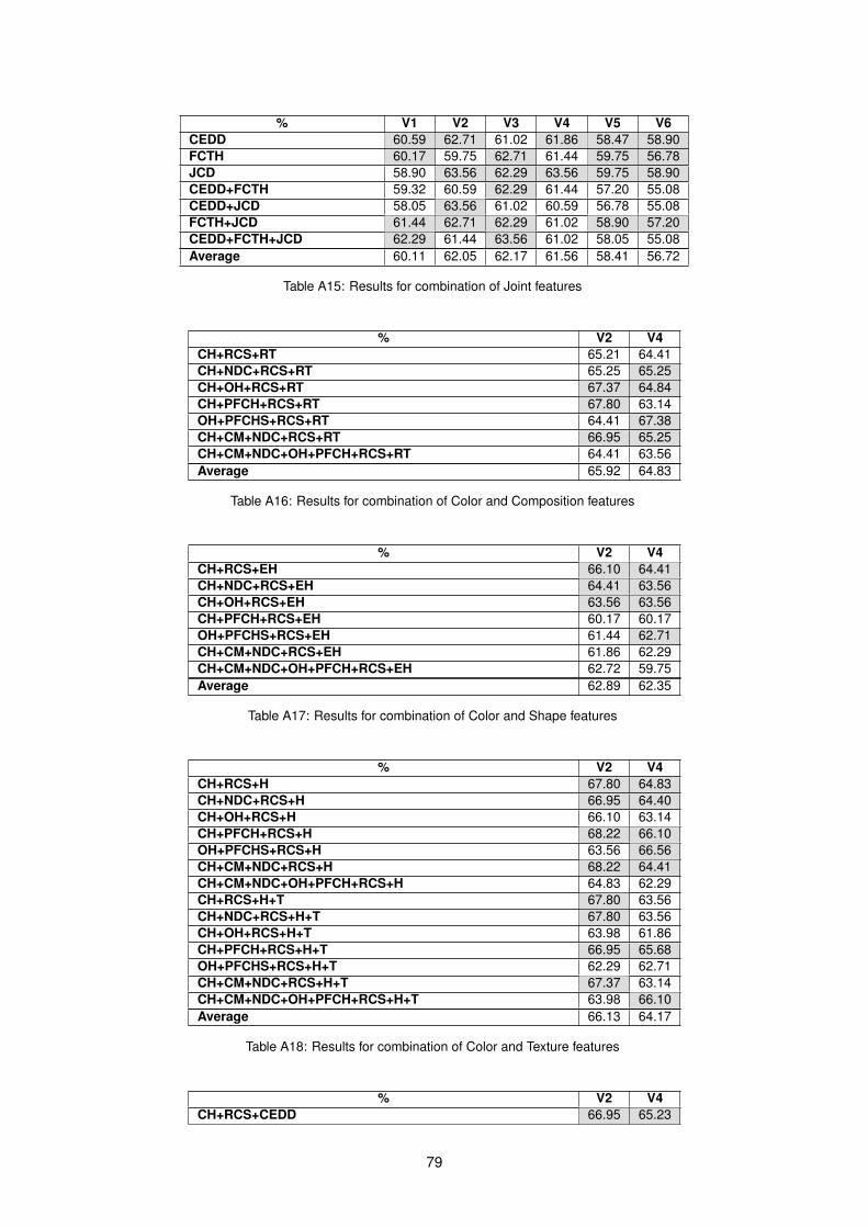
% V1 V2 V3 V4 V5 V6CEDD 60.59 62.71 61.02 61.86 58.47 58.90FCTH 60.17 59.75 62.71 61.44 59.75 56.78JCD 58.90 63.56 62.29 63.56 59.75 58.90CEDD+FCTH 59.32 60.59 62.29 61.44 57.20 55.08CEDD+JCD 58.05 63.56 61.02 60.59 56.78 55.08FCTH+JCD 61.44 62.71 62.29 61.02 58.90 57.20CEDD+FCTH+JCD 62.29 61.44 63.56 61.02 58.05 55.08Average 60.11 62.05 62.17 61.56 58.41 56.72

Table A15: Results for combination of Joint features

% V2 V4CH+RCS+RT 65.21 64.41CH+NDC+RCS+RT 65.25 65.25CH+OH+RCS+RT 67.37 64.84CH+PFCH+RCS+RT 67.80 63.14OH+PFCHS+RCS+RT 64.41 67.38CH+CM+NDC+RCS+RT 66.95 65.25CH+CM+NDC+OH+PFCH+RCS+RT 64.41 63.56Average 65.92 64.83

Table A16: Results for combination of Color and Composition features

% V2 V4CH+RCS+EH 66.10 64.41CH+NDC+RCS+EH 64.41 63.56CH+OH+RCS+EH 63.56 63.56CH+PFCH+RCS+EH 60.17 60.17OH+PFCHS+RCS+EH 61.44 62.71CH+CM+NDC+RCS+EH 61.86 62.29CH+CM+NDC+OH+PFCH+RCS+EH 62.72 59.75Average 62.89 62.35

Table A17: Results for combination of Color and Shape features

% V2 V4CH+RCS+H 67.80 64.83CH+NDC+RCS+H 66.95 64.40CH+OH+RCS+H 66.10 63.14CH+PFCH+RCS+H 68.22 66.10OH+PFCHS+RCS+H 63.56 66.56CH+CM+NDC+RCS+H 68.22 64.41CH+CM+NDC+OH+PFCH+RCS+H 64.83 62.29CH+RCS+H+T 67.80 63.56CH+NDC+RCS+H+T 67.80 63.56CH+OH+RCS+H+T 63.98 61.86CH+PFCH+RCS+H+T 66.95 65.68OH+PFCHS+RCS+H+T 62.29 62.71CH+CM+NDC+RCS+H+T 67.37 63.14CH+CM+NDC+OH+PFCH+RCS+H+T 63.98 66.10Average 66.13 64.17

Table A18: Results for combination of Color and Texture features

% V2 V4CH+RCS+CEDD 66.95 65.23

79

CH+NDC+RCS+CEDD 67.80 65.25CH+OH+RCS+CEDD 68.64 64.83CH+PFCH+RCS+CEDD 65.68 63.98OH+PFCHS+RCS+CEDD 63.98 61.02CH+CM+NDC+RCS+CEDD 67.37 63.98CH+CM+NDC+OH+PFCH+RCS+CEDD 66.10 62.71CH+RCS+JCD 65.25 65.25CH+NDC+RCS+JCD 65.25 64.83CH+OH+RCS+JCD 65.25 63.56CH+PFCH+RCS+JCD 62.29 63.56OH+PFCHS+RCS+JCD 64.41 61.12CH+CM+NDC+RCS+JCD 66.95 64.83CH+CM+NDC+OH+PFCH+RCS+JCD 63.56 59.75CH+RCS+FCTH+JCD 66.53 63.14CH+NDC+RCS+FCTH+JCD 65.23 64.83CH+OH+RCS+FCTH+JCD 65.25 63.56CH+PFCH+RCS+FCTH+JCD 62.29 63.56OH+PFCHS+RCS+FCTH+JCD 64.41 61.02CH+CM+NDC+RCS+FCTH+JCD 66.95 64.83CH+CM+NDC+OH+PFCH+RCS+FCTH+JCD 64.41 64.41Average 65.45 63.58

Table A19: Results for combination of Color and Joint features

% V2 V4RT+EH 47.88 52.12

Table A20: Results for combination of Composition and Shape features

% V2 V4RT+H 55.51 57.63RT+H+T 55.93 58.90Average 55.72 58.27

Table A21: Results for combination of Composition and Texture features

% V2 V4RT+CEDD 61.44 61.44RT+JCD 62.29 60.59RT+FCTH+JCD 62.71 59.32Average 62.15 60.45

Table A22: Results for combination of Composition and Joint features

% V2 V4EH + H 50.85 51.65EH + H + T 50.42 49.15Average 50.64 50.40

Table A23: Results for combination of Shape and Texture features

% V2 V4EH + CEDD 56.78 52.97EH + JCD 56.36 59.75EH + FCTH + JCD 57.63 57.63Average 56.92 56.78

80

Table A24: Results for combination of Shape and Joint features

% V2 V4H+CEDD 61.02 58.57H+JCD 59.32 56.78H+FCTH+JCD 58.47 60.17H+T+CEDD 60.59 59.32H+T+JCD 61.44 61.02H+T+FCTH+JCD 61.44 61.02Average 60.38 59.48

Table A25: Results for combination of Texture and Joint features

% V2 V4CH+RCS+RT+EH 62.29 61.02CH+NDC+RCS+RT+EH 63.98 61.02CH+OH+RCS+RT+EH 61.44 62.71CH+PFCH+RCS+RT+EH 63.98 61.02OH+PFCHS+RCS+RT+EH 62.29 63.98CH+CM+NDC+RCS+RT+EH 62.29 61.86CH+CM+NDC+OH+PFCH+RCS+RT+EH 61.86 59.32Average 62.59 61.56

Table A26: Results for combination of Color, Composition and Shape features

% V2 V4CH+RCS+RT+H 66.92 63.98CH+NDC+RCS+RT+H 66.10 65.25CH+OH+RCS+RT+H 64.41 63.98CH+PFCH+RCS+RT+H 66.53 64.41OH+PFCHS+RCS+RT+H 65.25 68.22CH+CM+NDC+RCS+RT+H 67.37 64.41CH+CM+NDC+OH+PFCH+RCS+RT+H 64.83 63.14CH+RCS+RT+H+T 66.95 63.98CH+NDC+RCS+RT+H+T 66.52 64.41CH+OH+RCS+RT+H+T 64.41 62.71CH+PFCH+RCS+RT+H+T 66.95 63.98OH+PFCHS+RCS+RT+H+T 66.95 66.56CH+CM+NDC+RCS+RT+H+T 66.10 64.83CH+CM+NDC+OH+PFCH+RCS+RT+H+T 66.10 65.25Average 66.10 64.65

Table A27: Results for combination of Color, Composition and Texture features

% V2 V4CH+RCS+RT+CEDD 63.98 61.86CH+NDC+RCS+RT+CEDD 67.37 62.71CH+OH+RCS+RT+CEDD 68.22 63.14CH+PFCH+RCS+RT+CEDD 63.14 60.59OH+PFCHS+RCS+RT+CEDD 61.44 61.86CH+CM+NDC+RCS+RT+CEDD 65.68 61.86CH+CM+NDC+OH+PFCH+RCS+RT+CEDD 66.52 61.44CH+RCS+RT+JCD 65.25 64.83CH+NDC+RCS+RT+JCD 65.68 63.98CH+OH+RCS+RT+JCD 66.10 64.41CH+PFCH+RCS+RT+JCD 66.10 63.98

81

OH+PFCHS+RCS+RT+JCD 63.56 61.44CH+CM+NDC+RCS+RT+JCD 65.68 63.14CH+CM+NDC+OH+PFCH+RCS+RT+JCD 65.25 63.98CH+RCS+RT+FCTH+JCD 65.25 64.83CH+NDC+RCS+RT+FCTH+JCD 65.68 63.98CH+OH+RCS+RT+FCTH+JCD 66.10 64.41CH+PFCH+RCS+RT+FCTH+JCD 66.10 63.98OH+PFCHS+RCS+RT+FCTH+JCD 61.86 60.17CH+CM+NDC+RCS+RT+FCTH+JCD 65.68 63.14CH+CM+NDC+OH+PFCH+RCS+RT+FCTH+JCD 64.83 63.56Average 65.21 63.01

Table A28: Results for combination of Color, Composition and Joint features

% V2 V4CH+RCS+EH+H 64.41 65.68CH+NDC+RCS+EH+H 65.25 65.68CH+OH+RCS+EH+H 62.71 63.98CH+PFCH+RCS+EH+H 63.14 63.56OH+PFCHS+RCS+EH+H 61.44 62.71CH+CM+NDC+RCS+EH+H 64.83 63.56CH+CM+NDC+OH+PFCH+RCS+EH+H 62.71 61.86CH+RCS+EH+H+T 62.29 63.29CH+NDC+RCS+EH+H+T 61.01 63.98CH+OH+RCS+EH+H+T 63.98 65.68CH+PFCH+RCS+EH+H+T 63.98 61.86OH+PFCHS+RCS+EH+H+T 63.14 62.71CH+CM+NDC+RCS+EH+H+T 63.14 63.98CH+CM+NDC+OH+PFCH+RCS+EH+H+T 63.98 62.29Average 63.29 63.63

Table A29: Results for combination of Color, Shape and Texture features

% V2 V4CH+RCS+EH+CEDD 62.71 62.71CH+NDC+RCS+EH+CEDD 63.56 62.29CH+OH+RCS+EH+CEDD 63.14 64.41CH+PFCH+RCS+EH+CEDD 62.71 59.75OH+PFCHS+RCS+EH+CEDD 60.59 59.75CH+CM+NDC+RCS+EH+CEDD 63.14 62.71CH+CM+NDC+OH+PFCH+RCS+EH+CEDD 62.29 59.32CH+RCS+EH+JCD 62.29 64.41CH+NDC+RCS+EH+JCD 61.44 63.98CH+OH+RCS+EH+JCD 63.14 61.86CH+PFCH+RCS+EH+JCD 62.29 61.86OH+PFCHS+RCS+EH+JCD 63.14 60.59CH+CM+NDC+RCS+EH+JCD 63.98 64.41CH+CM+NDC+OH+PFCH+RCS+EH+JCD 61.44 61.02CH+RCS+EH+FCTH+JCD 62.29 64.41CH+NDC+RCS+EH+FCTH+JCD 65.25 64.83CH+OH+RCS+EH+FCTH+JCD 62.71 63.14CH+PFCH+RCS+EH+FCTH+JCD 62.71 63.56OH+PFCHS+RCS+EH 61.44 62.71CH+CM+NDC+RCS+EH+FCTH+JCD 63.56 62.29CH+CM+NDC+OH+PFCH+RCS+EH+FCTH+JCD 62.29 60.59Average 62.67 62.41

Table A30: Results for combination of Color, Shape and Joint features

82

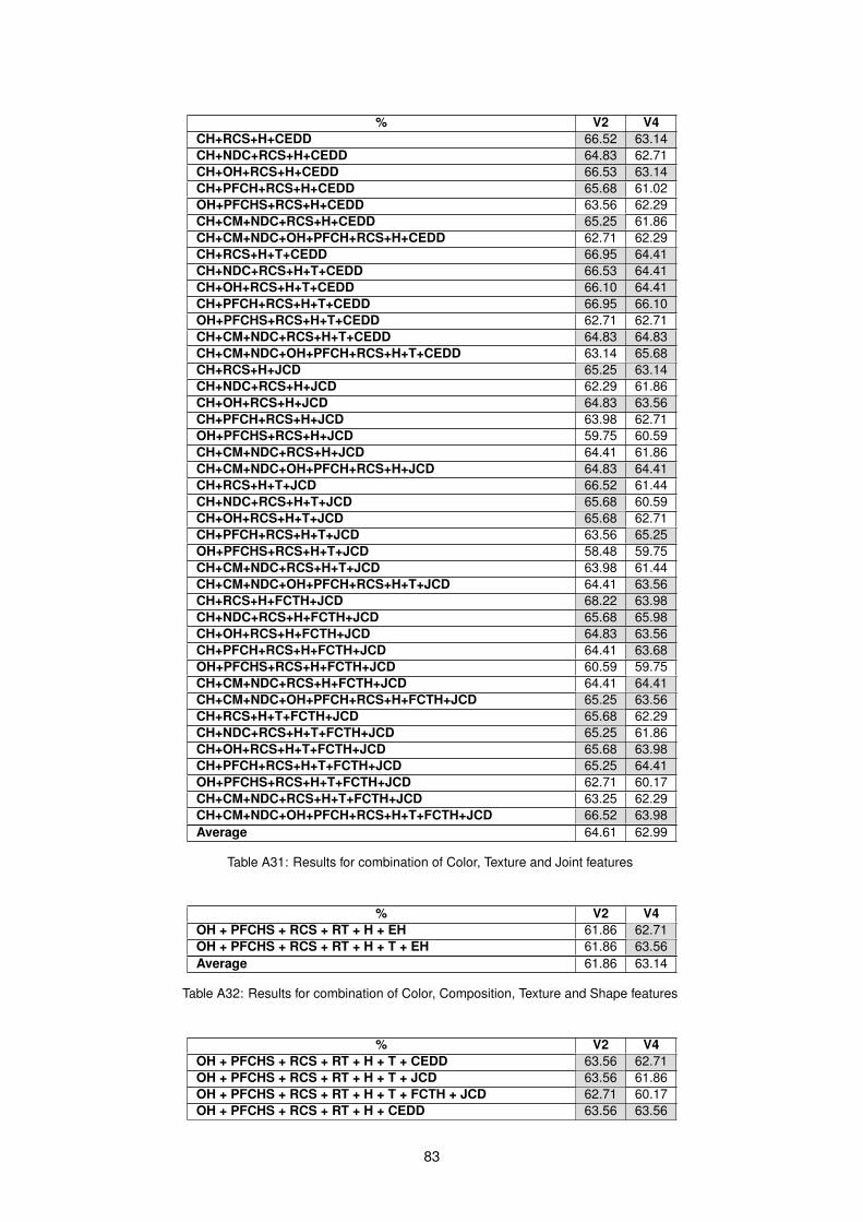
% V2 V4CH+RCS+H+CEDD 66.52 63.14CH+NDC+RCS+H+CEDD 64.83 62.71CH+OH+RCS+H+CEDD 66.53 63.14CH+PFCH+RCS+H+CEDD 65.68 61.02OH+PFCHS+RCS+H+CEDD 63.56 62.29CH+CM+NDC+RCS+H+CEDD 65.25 61.86CH+CM+NDC+OH+PFCH+RCS+H+CEDD 62.71 62.29CH+RCS+H+T+CEDD 66.95 64.41CH+NDC+RCS+H+T+CEDD 66.53 64.41CH+OH+RCS+H+T+CEDD 66.10 64.41CH+PFCH+RCS+H+T+CEDD 66.95 66.10OH+PFCHS+RCS+H+T+CEDD 62.71 62.71CH+CM+NDC+RCS+H+T+CEDD 64.83 64.83CH+CM+NDC+OH+PFCH+RCS+H+T+CEDD 63.14 65.68CH+RCS+H+JCD 65.25 63.14CH+NDC+RCS+H+JCD 62.29 61.86CH+OH+RCS+H+JCD 64.83 63.56CH+PFCH+RCS+H+JCD 63.98 62.71OH+PFCHS+RCS+H+JCD 59.75 60.59CH+CM+NDC+RCS+H+JCD 64.41 61.86CH+CM+NDC+OH+PFCH+RCS+H+JCD 64.83 64.41CH+RCS+H+T+JCD 66.52 61.44CH+NDC+RCS+H+T+JCD 65.68 60.59CH+OH+RCS+H+T+JCD 65.68 62.71CH+PFCH+RCS+H+T+JCD 63.56 65.25OH+PFCHS+RCS+H+T+JCD 58.48 59.75CH+CM+NDC+RCS+H+T+JCD 63.98 61.44CH+CM+NDC+OH+PFCH+RCS+H+T+JCD 64.41 63.56CH+RCS+H+FCTH+JCD 68.22 63.98CH+NDC+RCS+H+FCTH+JCD 65.68 65.98CH+OH+RCS+H+FCTH+JCD 64.83 63.56CH+PFCH+RCS+H+FCTH+JCD 64.41 63.68OH+PFCHS+RCS+H+FCTH+JCD 60.59 59.75CH+CM+NDC+RCS+H+FCTH+JCD 64.41 64.41CH+CM+NDC+OH+PFCH+RCS+H+FCTH+JCD 65.25 63.56CH+RCS+H+T+FCTH+JCD 65.68 62.29CH+NDC+RCS+H+T+FCTH+JCD 65.25 61.86CH+OH+RCS+H+T+FCTH+JCD 65.68 63.98CH+PFCH+RCS+H+T+FCTH+JCD 65.25 64.41OH+PFCHS+RCS+H+T+FCTH+JCD 62.71 60.17CH+CM+NDC+RCS+H+T+FCTH+JCD 63.25 62.29CH+CM+NDC+OH+PFCH+RCS+H+T+FCTH+JCD 66.52 63.98Average 64.61 62.99

Table A31: Results for combination of Color, Texture and Joint features

% V2 V4OH + PFCHS + RCS + RT + H + EH 61.86 62.71OH + PFCHS + RCS + RT + H + T + EH 61.86 63.56Average 61.86 63.14

Table A32: Results for combination of Color, Composition, Texture and Shape features

% V2 V4OH + PFCHS + RCS + RT + H + T + CEDD 63.56 62.71OH + PFCHS + RCS + RT + H + T + JCD 63.56 61.86OH + PFCHS + RCS + RT + H + T + FCTH + JCD 62.71 60.17OH + PFCHS + RCS + RT + H + CEDD 63.56 63.56

83

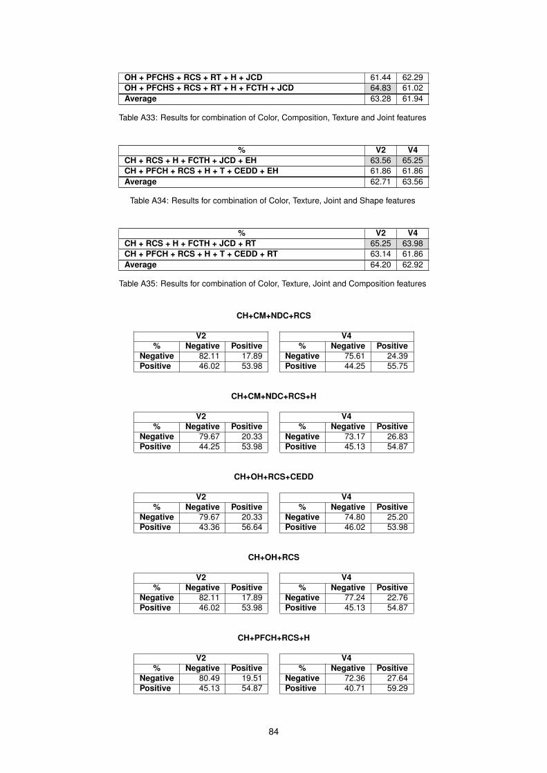
OH + PFCHS + RCS + RT + H + JCD 61.44 62.29OH + PFCHS + RCS + RT + H + FCTH + JCD 64.83 61.02Average 63.28 61.94

Table A33: Results for combination of Color, Composition, Texture and Joint features

% V2 V4CH + RCS + H + FCTH + JCD + EH 63.56 65.25CH + PFCH + RCS + H + T + CEDD + EH 61.86 61.86Average 62.71 63.56

Table A34: Results for combination of Color, Texture, Joint and Shape features

% V2 V4CH + RCS + H + FCTH + JCD + RT 65.25 63.98CH + PFCH + RCS + H + T + CEDD + RT 63.14 61.86Average 64.20 62.92

Table A35: Results for combination of Color, Texture, Joint and Composition features

CH+CM+NDC+RCS

V2 V4% Negative Positive % Negative Positive

Negative 82.11 17.89 Negative 75.61 24.39Positive 46.02 53.98 Positive 44.25 55.75

CH+CM+NDC+RCS+H

V2 V4% Negative Positive % Negative Positive

Negative 79.67 20.33 Negative 73.17 26.83Positive 44.25 53.98 Positive 45.13 54.87

CH+OH+RCS+CEDD

V2 V4% Negative Positive % Negative Positive

Negative 79.67 20.33 Negative 74.80 25.20Positive 43.36 56.64 Positive 46.02 53.98

CH+OH+RCS

V2 V4% Negative Positive % Negative Positive

Negative 82.11 17.89 Negative 77.24 22.76Positive 46.02 53.98 Positive 45.13 54.87

CH+PFCH+RCS+H

V2 V4% Negative Positive % Negative Positive

Negative 80.49 19.51 Negative 72.36 27.64Positive 45.13 54.87 Positive 40.71 59.29

84

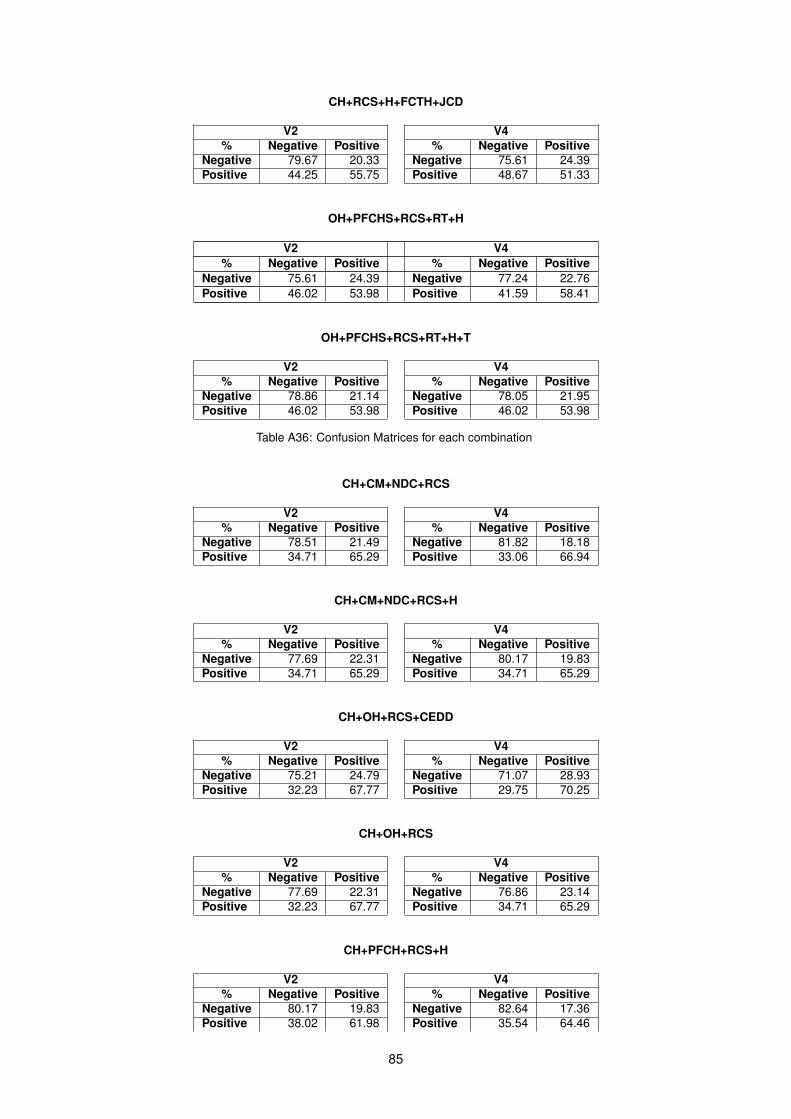
CH+RCS+H+FCTH+JCD

V2 V4% Negative Positive % Negative Positive

Negative 79.67 20.33 Negative 75.61 24.39Positive 44.25 55.75 Positive 48.67 51.33

OH+PFCHS+RCS+RT+H

V2 V4% Negative Positive % Negative Positive

Negative 75.61 24.39 Negative 77.24 22.76Positive 46.02 53.98 Positive 41.59 58.41

OH+PFCHS+RCS+RT+H+T

V2 V4% Negative Positive % Negative Positive

Negative 78.86 21.14 Negative 78.05 21.95Positive 46.02 53.98 Positive 46.02 53.98

Table A36: Confusion Matrices for each combination

CH+CM+NDC+RCS

V2 V4% Negative Positive % Negative Positive

Negative 78.51 21.49 Negative 81.82 18.18Positive 34.71 65.29 Positive 33.06 66.94

CH+CM+NDC+RCS+H

V2 V4% Negative Positive % Negative Positive

Negative 77.69 22.31 Negative 80.17 19.83Positive 34.71 65.29 Positive 34.71 65.29

CH+OH+RCS+CEDD

V2 V4% Negative Positive % Negative Positive

Negative 75.21 24.79 Negative 71.07 28.93Positive 32.23 67.77 Positive 29.75 70.25

CH+OH+RCS

V2 V4% Negative Positive % Negative Positive

Negative 77.69 22.31 Negative 76.86 23.14Positive 32.23 67.77 Positive 34.71 65.29

CH+PFCH+RCS+H

V2 V4% Negative Positive % Negative Positive

Negative 80.17 19.83 Negative 82.64 17.36Positive 38.02 61.98 Positive 35.54 64.46

85

CH+RCS+H+FCTH+JCD

V2 V4% Negative Positive % Negative Positive

Negative 78.51 21.49 Negative 76.86 23.14Positive 35.54 64.46 Positive 32.23 67.77

OH+PFCHS+RCS+RT+H

V2 V4% Negative Positive % Negative Positive

Negative 75.21 24.79 Negative 76.86 23.14Positive 34.71 65.29 Positive 33.88 66.12

OH+PFCHS+RCS+RT+H+T

V2 V4% Negative Positive % Negative Positive

Negative 76.03 23.97 Negative 77.69 22.31Positive 32.23 67.77 Positive 33.88 66.12

Table A37: Confusion Matrices for each combination using GAPED dataset with Negative and Positive categories

CH+CM+NDC+RCS

V2 V4% Negative Neutral Positive % Negative Neutral Positive

Negative 51.24 28.93 19.83 Negative 37.19 44.63 18.18Neutral 33.71 49.44 16.85 Neutral 24.72 62.92 12.36Positive 23.97 22.31 53.72 Positive 22.31 29.75 47.93

CH+CM+NDC+RCS+H

V2 V4% Negative Neutral Positive % Negative Neutral Positive

Negative 61.16 18.18 20.66 Negative 51.24 31.41 17.36Neutral 23.60 57.30 19.19 Neutral 25.84 62.92 11.24Positive 27.27 21.49 51.24 Positive 25.62 27.27 47.11

CH+OH+RCS+CEDD

V2 V4% Negative Neutral Positive % Negative Neutral Positive

Negative 55.37 21.49 23.14 Negative 58.68 22.31 19.01Neutral 22.47 59.55 17.98 Neutral 24.72 64.04 11.24Positive 23.14 22.31 54.55 Positive 21.49 26.45 52.07

CH+OH+RCS

V2 V4% Negative Neutral Positive % Negative Neutral Positive

Negative 37.19 47.11 15.70 Negative 37.19 47.11 15.70Neutral 30.34 56.18 13.48 Neutral 30.34 56.18 13.48Positive 23.97 29.75 46.28 Positive 23.97 29.75 46.28

86

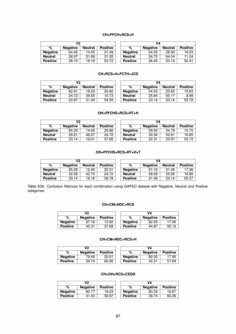
CH+PFCH+RCS+H

V2 V4% Negative Neutral Positive % Negative Neutral Positive

Negative 64.46 14.05 21.49 Negative 54.55 28.93 16.53Neutral 26.97 51.69 21.35 Neutral 24.72 64.04 11.24Positive 28.10 18.18 53.72 Positive 26.45 23.14 50.41

CH+RCS+H+FCTH+JCD

V2 V4% Negative Neutral Positive % Negative Neutral Positive

Negative 62.81 16.53 20.66 Negative 54.55 25.62 19.83Neutral 24.72 59.55 15.73 Neutral 25.84 65.17 8.99Positive 23.97 21.49 54.55 Positive 23.14 23.14 53.72

OH+PFCHS+RCS+RT+H

V2 V4% Negative Neutral Positive % Negative Neutral Positive

Negative 65.29 14.05 20.66 Negative 59.50 24.79 15.70Neutral 29.21 46.07 24.72 Neutral 30.34 52.81 16.85Positive 23.14 19.01 57.85 Positive 22.31 23.97 53.72

OH+PFCHS+RCS+RT+H+T

V2 V4% Negative Neutral Positive % Negative Neutral Positive

Negative 65.29 12.40 22.31 Negative 61.16 21.49 17.36Neutral 32.58 42.70 24.72 Neutral 28.09 55.06 16.85Positive 23.14 18.18 58.78 Positive 21.49 23.14 55.37

Table A38: Confusion Matrices for each combination using GAPED dataset with Negative, Neutral and Positivecategories

CH+CM+NDC+RCS

V2 V4% Negative Positive % Negative Positive

Negative 87.18 12.82 Negative 82.05 17.95Positive 42.31 57.69 Positive 44.87 55.13

CH+CM+NDC+RCS+H

V2 V4% Negative Positive % Negative Positive

Negative 79.49 20.51 Negative 82.05 17.95Positive 39.74 60.26 Positive 42.31 57.69

CH+OH+RCS+CEDD

V2 V4% Negative Positive % Negative Positive

Negative 80.77 19.23 Negative 83.33 16.67Positive 41.03 58.97 Positive 39.74 60.26

87

CH+OH+RCS

V2 V4% Negative Positive % Negative Positive

Negative 78.21 21.79 Negative 75.64 24.36Positive 43.59 56.41 Positive 46.15 53.85

CH+PFCH+RCS+H

V2 V4% Negative Positive % Negative Positive

Negative 80.77 19.23 Negative 79.49 20.51Positive 39.74 60.26 Positive 43.59 56.41

CH+RCS+H+FCTH+JCD

V2 V4% Negative Positive % Negative Positive

Negative 79.49 20.51 Negative 85.90 14.10Positive 38.47 61.54 Positive 44.87 55.13

OH+PFCHS+RCS+RT+H

V2 V4% Negative Positive % Negative Positive

Negative 82.05 17.95 Negative 87.18 12.82Positive 44.87 55.13 Positive 47.45 52.56

OH+PFCHS+RCS+RT+H+T

V2 V4% Negative Positive % Negative Positive

Negative 85.90 14.10 Negative 88.50 11.54Positive 43.59 56.41 Positive 46.15 53.85

Table A39: Confusion Matrices for each combination using Mikels and GAPED dataset

88

Appendix B

Questionnaire

89

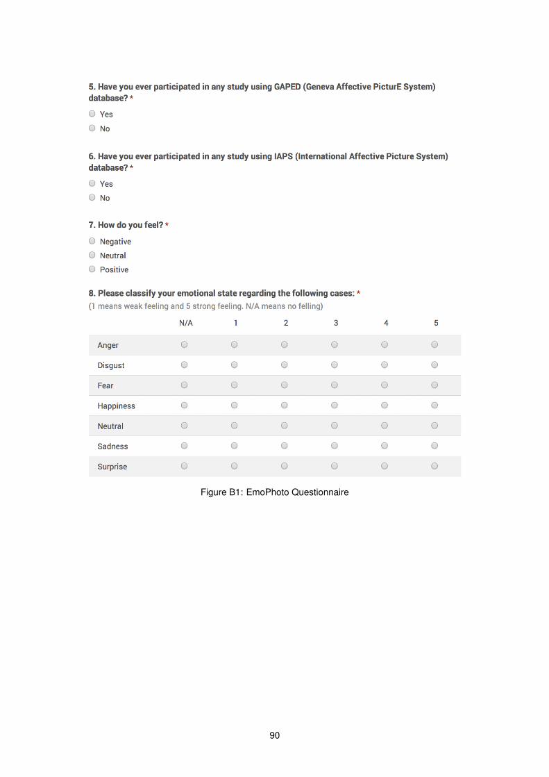
Figure B1: EmoPhoto Questionnaire

90

Results of the Questionnaire

Figure B2: 1. Age

Figure B3: 2. Gender

91

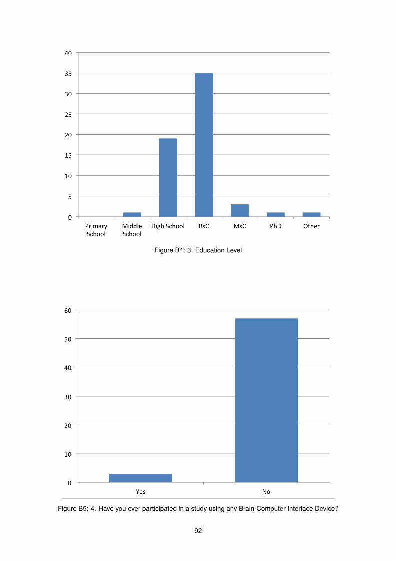
Figure B4: 3. Education Level

Figure B5: 4. Have you ever participated in a study using any Brain-Computer Interface Device?

92

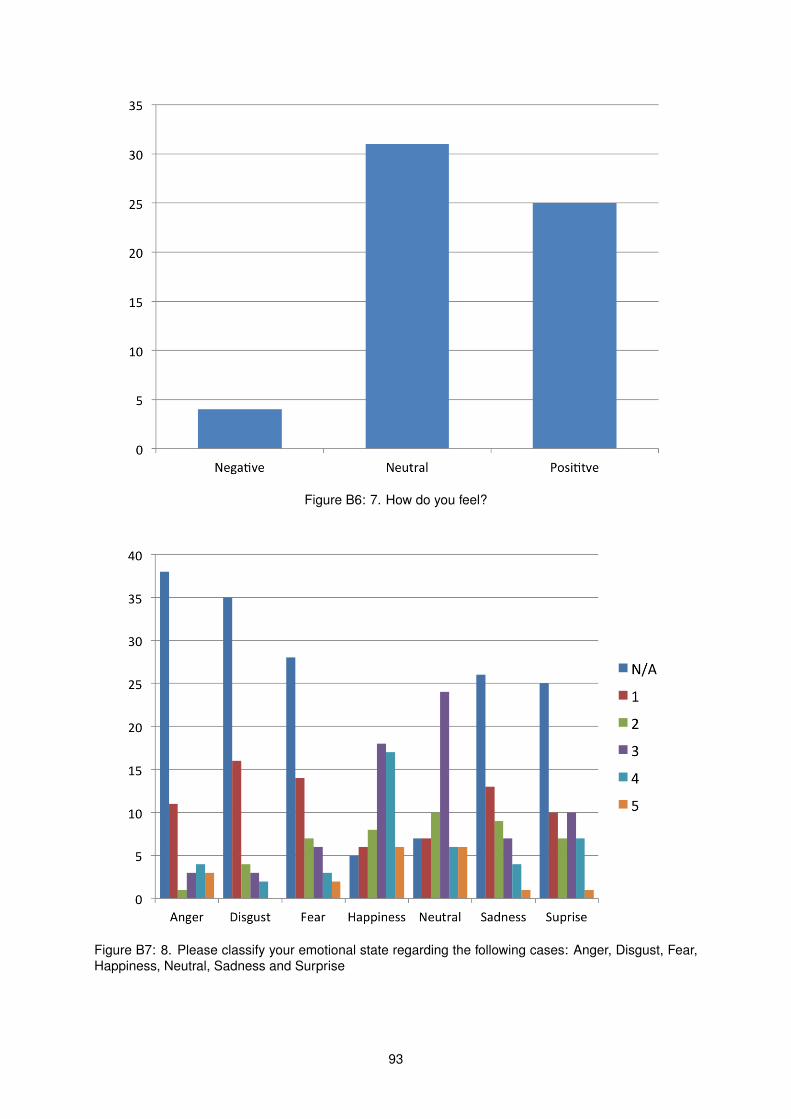
Figure B6: 7. How do you feel?

Figure B7: 8. Please classify your emotional state regarding the following cases: Anger, Disgust, Fear,Happiness, Neutral, Sadness and Surprise

93

94