iii

EMERGY SYNTHESIS 6: Theory and Applications of the Emergy Methodology

Proceedings from the Sixth Biennial Emergy Conference,

January 14 – 16, 2010, Gainesville, Florida

Edited by

Mark T. Brown University of Florida

Gainesville, Florida

Managing Editor

Sharlynn Sweeney University of Florida

Gainesville, Florida

Associate Editors

Daniel E. Campbell US EPA

Narragansett, Rhode Island

Shu-Li Huang National Taipei University

Taipei, Taiwan

Enrique Ortega State University of Campinas

Campinas, Brazil

Torbjörn Rydberg Centre for Sustainable Agriculture

Uppsala, Sweden

David Tilley University of Maryland

College Park, Maryland

Sergio Ulgiati Parthenope University of Napoli

Napoli, Italy

December 2011

The Center for Environmental Policy Department of Environmental Engineering Sciences

University of Florida

Gainesville, FL

539

45

Assessing Geobiosphere Work of Generating Global Reserves of

Coal, Crude Oil and Natural Gas

Mark Brown, Gaetano Protano, and Sergio Ulgiati

ABSTRACT

A teacher of ours used to say, “Like ice in a fire, something for nothing you will never acquire”,

which is a poetic equivalent of “there is no such a thing as a free lunch”. Human economies are

dependent on high quality fossil fuels and will likely continue depending on them for some time to

come. Value of a resource is not only what one pays for it, or what can be extracted from it, but also

value can be attributed to the “effort” required in its production. In this analysis we apply the emergy

synthesis method to evaluate the work invested by the geobiosphere to generate the global storages of

fossil energy resources. The upgrading of raw resources to secondary fuels is also evaluated. The

analysis relies on published estimates of historic, global net primary production (NPP) on land and

oceans, published preservation and conversion factors of organic matter, and assessments of the

present total global storages of coal, petroleum, and natural gas. Results show that the production of

coal resources over geologic time required between 6.63 E4 (+/-0.51 E4) seJ/J and 9.71 E4 (+/-0.79

E4) seJ/J, while, oil and natural gas resources required about 1.48 E5 (+/- 0.07 E5) seJ/J and 1.71 E5

(+/- 0.06 E5) seJ/J, respectively. These values are between 1.5 to 2.5 times larger than previous

estimates and acknowledge a far greater power of fossil fuels in driving and shaping modern society.

INTRODUCTION

Fossil fuels are important. Human society depends on them and will likely continue doing so for

many decades to come, in spite of concerns for climate change, peak oil, increasing prices, and

national security. We are well aware of the importance of fossil fuels and as a consequence need to

assign an energetic and environmental value that is commensurate with their quality. That different

energies have different qualities and thus have different costs of production and abilities to do work is

a major conceptual principle of the Emergy Synthesis methodology (Odum, 1988; Odum, 1996;

Brown and Ulgiati, 1997; Brown and Ulgiati, 2004). This principle is the foundation of the concept of

transformity and specific emergy. Transformity (in units of seJ/J) and specific emergy (in units of

seJ/g) are examples of the more general term, Unit Emergy Value (UEVs), which is defined as the

ratio of available emergy of one type (emergy) that is required directly or indirectly to produce a unit

output from a process. UEVs are ratios that allow the conversion of different forms of energy into a

single form named emergy.

Within the framework of Emergy Synthesis the quality of energy (and any other resource) is

measured by the inputs of energy, materials and information required to make it. The unit emergy

value (UEV) is a measure of those inputs when the inputs are expressed in the same units. UEVs for

the fossil fuels are extremely important as they form the basis for the calculation of most second order

energies (eg , electricity), products, and services. It has long been recognized that there is no single

Unit Emergy Value (UEV) for a particular substance or product as there are a multitude of possible

processes that can produce them (Brown and Ulgiati, 2004). Yet emergy analysts often use a single

UEV assuming that the differences in UEVs are negligible (which is sometimes the case) or that the

particular published UEV value is representative of a larger set of values. However, relying on a

540

single UEV from a single case study is less than desirable because it may not always be representative

of the global set of processes that lead to a given product. A weighted average of many processes that

yield the same product would be a much more preferable option if the actual source of an input is not

known.

There have been previous evaluations of the UEVs for fossil fuels, first by Odum (1996) and

more recently by Bastianoni et al. (2005). In both instances the evaluations were based on a single

case study. Odum (1996) reported interdependent transformities for oil, natural gas, and coal using a

technique of back calculation from the transformity of electric power plants and assumption of the

relative efficiencies of coal and oil thermal plants. Bastianoni et al. (2005) computed the transformity

and specific emergy of oil and petroleum natural gas based on the biogeochemical processes that

contributed to their formation in a particular site, located in Russia, which was suggested as the most

productive oil formation site known, translating into conservative UEV estimates. However, they

included only the biological processes and did not include the additional geothermal ―treatment‖ that is

a necessary input to convert the buried biomass into kerogen and finally oil and gas.

In this study we carry the analysis further by using the total known conventional reserves of oil1,

natural gas, and coal over geological ages, and separating the production process into two separate

processes governed first by biological process and second by geothermal processes. By separating the

processes, we compute the emergy required to produce the organic matter, which is the precursor to

kerogen and then the geothermal emergy required to generate the final product.

METHODS

The production of coal and petroleum are similar in that there is a biological phase and a

geothermal phase, yet the biological phases differ since the source for coal is largely peat derived from

terrestrial production and petroleum’s sources are largely of marine origin; therefore we evaluate their

UEVs separately.

Coal

There are two very distinct processes that contribute to coal formation (Figure 1). The first phase

is the production of living biomass and accumulation of partially decomposed organic matter that is

transformed through a second phase of coalification. Both phases are separated in time and in space,

since ecological production ceases at some point and the accumulated organic matter is buried to

achieve the second geothermal phase. The first phase, the ecological phase, is driven by the energy

and ecological processes that support primary production, while geothermal processes drive the second

phase (accumulation and further processing). Determination of the emergy driving the formation of

coal is divided into these two phases accordingly. In addition to evaluating the two phases, we also

evaluated the coal resource based on geologic age and also divided the coal resource into hard coal

(anthracite/ bituminous = 53% of total resource) and soft coal (sub-bituminous/lignite= 47% of total

resource) based on estimates by the Energy Information Administration (EIA, 2008). Table 1 lists the

quantity and available energy of the hard and soft coal resource by geologic age. The low coal

productivity shown by Devonian period is likely due to still incomplete colonization of continents by

organisms and therefore an insufficient amount of terrestrial peat-forming biomass; the similar low

productivity in the Triassic can be attributed to the well known "coal gap". i.e. the extinction of peat-

forming plants at the end of the Permian, about 250 Ma ago (Retallack et al., 1996; Beerling, 2002).

Phase 1: Net Primary Production to Peat

It is generally accepted that coal was formed from terrestrial sources, largely in prehistoric swamps

(Teichmuller & Teichmuller, 1986). The anoxic and acidic environment of wetland soils resulted in

relatively slow decomposition of organic matter leading to its accumulation over time in large deposits

1 Unless otherwise stated, in this analysis the term oil means crude oil throughout.

541

of peat. In modern times, accumulation rates of peat in swamps average about 2.5 mm/yr. In some

geologic ages accumulation may well have been higher. Rather than trying to estimate accumulation

rates, in this analysis, we use estimates from the literature of the coal resource that was produced in

each geologic age and back calculate the Net Primary Production (NPP) that was required, using the

preservation factors (PFs) or efficiencies of conversion. Following Dukes (2003), a preservation factor

is the fraction of carbon that remains at the end of a transition from one fossil fuel precursor to the

next, for example the fraction remaining from plant matter to peat, on the path to coal formation.

Shown in Figure 1 are two stages in the formation of the coal resource where PFs were applied (PF1,

PF2a, and PF2b). The preservation factors used in calculating NPP requirement for hard and soft coal

were based on literature values and are given in Table 2.

The first PF is the percent of organic matter that is preserved as peat. Dukes (2003) suggested

that preservation of organic matter in peat could range from 4% up to a high 39%, while Tissot and

Welte (1984) estimated it at less than 10%. Frolking et al. (2010) suggested a value around 6.5% based

on a 8500 yr Holocene Peat Model (HPM) of peat accumulation with carbon-water feedbacks in

Ontario, Canada. In our analysis we use 7% as a reasonable estimate extracted from these two sources.

The emergy required for the NPP in each geologic age was derived from literature sources

related to the global NPP in each age and assuming constant global emergy driving all Earth processes

of 15.2 E24 seJ/yr (Brown and Ulgiati, 2010). Table 3 lists the geologic ages, estimated NPP in each

age, and UEVs of NPP. The Specific Emergy of NPP ranges from 0.89 E7 to 3.55 E7 seJ/gC. NPPs

and UEVs for Devonian and Triassic are not much different than for the other ages; their low coal

production was therefore not due to insufficient amount of biomass, but instead more likely to

unsuitable characteristics and (for Triassic) early extinction of peat-forming plants.

Figure 1. The two phases of coal formation. Phase I: peat production is dominated by ecological

processes that are driven by solar, tidal, and geothermal energies of the geobiosphere. Phase II:

coalification is driven by geothermal energy. PF1-2 are preservation factors (fraction of carbon that is

preserved and passed to the next step): PF1 is the preservation between organic matter production and

peat accumulation. Hard coal and soft coal have two different preservation factors PF2a and PF2b

between peat and coal.

542

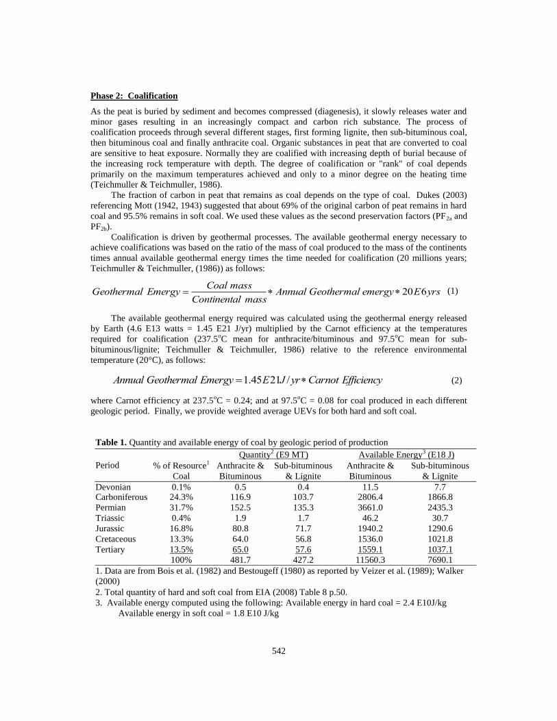
Phase 2: Coalification

As the peat is buried by sediment and becomes compressed (diagenesis), it slowly releases water and

minor gases resulting in an increasingly compact and carbon rich substance. The process of

coalification proceeds through several different stages, first forming lignite, then sub-bituminous coal,

then bituminous coal and finally anthracite coal. Organic substances in peat that are converted to coal

are sensitive to heat exposure. Normally they are coalified with increasing depth of burial because of

the increasing rock temperature with depth. The degree of coalification or "rank" of coal depends

primarily on the maximum temperatures achieved and only to a minor degree on the heating time

(Teichmuller & Teichmuller, 1986).

The fraction of carbon in peat that remains as coal depends on the type of coal. Dukes (2003)

referencing Mott (1942, 1943) suggested that about 69% of the original carbon of peat remains in hard

coal and 95.5% remains in soft coal. We used these values as the second preservation factors (PF2a and

PF2b).

Coalification is driven by geothermal processes. The available geothermal energy necessary to

achieve coalifications was based on the ratio of the mass of coal produced to the mass of the continents

times annual available geothermal energy times the time needed for coalification (20 millions years;

Teichmuller & Teichmuller, (1986)) as follows:

Geothermal Emergy Coal mass

Continental mass Annual Geothermal emergy 20E6yrs (1)

The available geothermal energy required was calculated using the geothermal energy released

by Earth (4.6 E13 watts = 1.45 E21 J/yr) multiplied by the Carnot efficiency at the temperatures

required for coalification (237.5oC mean for anthracite/bituminous and 97.5

oC mean for sub-

bituminous/lignite; Teichmuller & Teichmuller, 1986) relative to the reference environmental

temperature (20°C), as follows:

Annual Geothermal Emergy 1.45E21J /yrCarnot Efficiency (2)

where Carnot efficiency at 237.5oC = 0.24; and at 97.5

oC = 0.08 for coal produced in each different

geologic period. Finally, we provide weighted average UEVs for both hard and soft coal.

Table 1. Quantity and available energy of coal by geologic period of production

Period

Quantity2 (E9 MT) Available Energy

3 (E18 J)

% of Resource1

Coal

Anthracite &

Bituminous

Sub-bituminous

& Lignite

Anthracite &

Bituminous

Sub-bituminous

& Lignite

Devonian 0.1% 0.5 0.4 11.5 7.7 Carboniferous 24.3% 116.9 103.7 2806.4 1866.8

Permian 31.7% 152.5 135.3 3661.0 2435.3

Triassic 0.4% 1.9 1.7 46.2 30.7

Jurassic 16.8% 80.8 71.7 1940.2 1290.6

Cretaceous 13.3% 64.0 56.8 1536.0 1021.8

Tertiary 13.5% 65.0 57.6 1559.1 1037.1

100% 481.7 427.2 11560.3 7690.1

1. Data are from Bois et al. (1982) and Bestougeff (1980) as reported by Veizer et al. (1989); Walker

(2000)

2. Total quantity of hard and soft coal from EIA (2008) Table 8 p.50.

3. Available energy computed using the following: Available energy in hard coal = 2.4 E10J/kg

Available energy in soft coal = 1.8 E10 J/kg

543

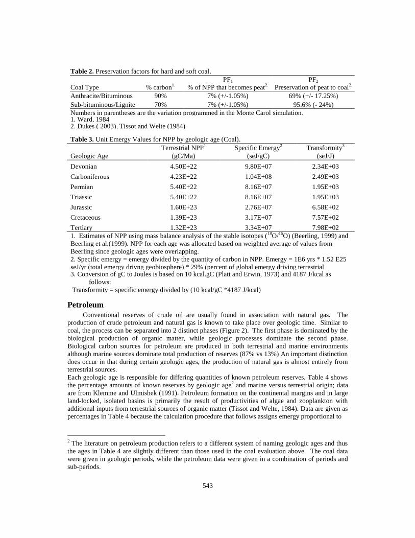
Table 2. Preservation factors for hard and soft coal.

Coal Type % carbon1.

PF1

% of NPP that becomes peat2.

PF2

Preservation of peat to coal2.

Anthracite/Bituminous 90% 7% (+/-1.05%) 69% (+/- 17.25%)

Sub-bituminous/Lignite 70% 7% (+/-1.05%) 95.6% (- 24%)

Numbers in parentheses are the variation programmed in the Monte Carol simulation. 1. Ward, 1984 2. Dukes ( 2003), Tissot and Welte (1984)

Table 3. Unit Emergy Values for NPP by geologic age (Coal).

Geologic Age

Terrestrial NPP1 Specific Emergy

2 Transformity

3

(gC/Ma) (seJ/gC) (seJ/J)

Devonian 4.50E+22 9.80E+07 2.34E+03

Carboniferous 4.23E+22 1.04E+08 2.49E+03

Permian 5.40E+22 8.16E+07 1.95E+03

Triassic 5.40E+22 8.16E+07 1.95E+03

Jurassic 1.60E+23 2.76E+07 6.58E+02

Cretaceous 1.39E+23 3.17E+07 7.57E+02

Tertiary 1.32E+23 3.34E+07 7.98E+02

1. Estimates of NPP using mass balance analysis of the stable isotopes (18

O/16

O) (Beerling, 1999) and

Beerling et al.(1999). NPP for each age was allocated based on weighted average of values from

Beerling since geologic ages were overlapping.

2. Specific emergy = emergy divided by the quantity of carbon in NPP. Emergy = 1E6 yrs * 1.52 E25

seJ/yr (total emergy drivng geobiosphere) * 29% (percent of global emergy driving terrestrial

production) = 4.4 E30 seJ/Ma 3. Conversion of gC to Joules is based on 10 kcal.gC (Platt and Erwin, 1973) and 4187 J/kcal as

follows:

Transformity = specific emergy divided by (10 kcal/gC *4187 J/kcal)

Petroleum

Conventional reserves of crude oil are usually found in association with natural gas. The

production of crude petroleum and natural gas is known to take place over geologic time. Similar to

coal, the process can be separated into 2 distinct phases (Figure 2). The first phase is dominated by the

biological production of organic matter, while geologic processes dominate the second phase.

Biological carbon sources for petroleum are produced in both terrestrial and marine environments

although marine sources dominate total production of reserves (87% vs 13%) An important distinction

does occur in that during certain geologic ages, the production of natural gas is almost entirely from

terrestrial sources.

Each geologic age is responsible for differing quantities of known petroleum reserves. Table 4 shows

the percentage amounts of known reserves by geologic age2 and marine versus terrestrial origin; data

are from Klemme and Ulmishek (1991). Petroleum formation on the continental margins and in large

land-locked, isolated basins is primarily the result of productivities of algae and zooplankton with

additional inputs from terrestrial sources of organic matter (Tissot and Welte, 1984). Data are given as

percentages in Table 4 because the calculation procedure that follows assigns emergy proportional to

2 The literature on petroleum production refers to a different system of naming geologic ages and thus

the ages in Table 4 are slightly different than those used in the coal evaluation above. The coal data

were given in geologic periods, while the petroleum data were given in a combination of periods and

sub-periods.

544

Figure 2. The two phases of petroleum formation. Phase I: organic matter production is dominated by

ecological processes driven by solar, tidal and geothermal energies of the geobiosphere. Phase II:

petroleum production is driven by geothermal energy. PF1-3 are preservation factors (fraction of

carbon that is preserved and passed to the next step): PF1is the preservation between organic matter

production and organic matter accumulation in basins, PF2 is the preservation between accumulated

organic matter and kerogen, and PF3 is the preservation between kerogen and oil/natural gas. (KI =

kerogen type I; KII = kerogen type II, KIII = kerogen type III).

* Data are from Klemme, H.D. and G. F. Ulmishek, 1991. Percentages do not add to 100% because

8.5% of global reserves produced in a number of miscellaneous time periods not included.

Table 4. Percent of known global reserves of petroleum hydrocarbons generated by geologic age

Geological Age

Geological

ages (Ma,

million years)

before present

Percent of

hydrocarbons

generated*

Percent of hydrocarbons generated per kerogen

type

From kerogen types I

& II (mainly marine)

From kerogen type III

(mainly terrestrial)

From To Oil Natural Gas Oil Natural Gas

Silurian 438 408 9.0% 15% 85% = =

Upper Devonian-

Turonian 374 352 8.0% 80% 20% = =

Pennsylvanian -

Lower Permian 320 286 8.0% 35% 43% = 22%

Upper Jurassic 169 144 25.0% 74% 26% = =

Middle Cretaceous 119 88.5 29.0% 61% 10% 4% 25%

Oligocene-Miocene 36.6 5.3 12.5% 28% 7% 39% 26%

545

the fraction of NPP that becomes hydrocarbons. The absolute amounts of hydrocarbons do not affect

the final emergy results, while percentages of total resource per age will have an effect. We also

assume that percentages of hydrocarbons generated in each geological age will not be appreciably

changed by new discoveries or more accurate estimates of total resource.

Phase I: Net Primary Production to Organic Sediments

In this phase of the evolution of petroleum, biological net primary production (NPP), which

converts biosphere energies into organic matter is the main process. As in the coal calculation, we

begin with the quantity of petroleum and natural gas that was produced in each geologic age and back

calculated to the quantity of NPP that was required to produce it using preservation and conservation

factors from literature. Table 5 lists the conversion factors for marine and terrestrial carbon becoming

hydrocarbons (the numbers in parentheses are percent variation used in Monte Carlo simulations,

below). The conversion efficiencies are based on data from Tissot and Welte (1984). The second and

third columns in the table list the percent of NPP from marine and terrestrial sources that is preserved

as kerogen. The fourth and fifth columns list the percent of marine and terrestrial kerogen that is

converted to hydrocarbons. Tissot and Welte show that for the most part, organic matter from marine

sources becomes kerogen types I and II, while terrestrial organic matter becomes kerogen type III. It

can be seen from Table 5 that the conversion efficiencies of terrestrial organic matter are much lower

than those for organic matter derived from marine NPP. This is an important consideration and has

significant impact on overall transformities, which we will address in the discussion

We allocate the emergy driving the geobiosphere (sum of solar radiation, tidal momentum and

geothermal energy: 15.2 E24 sej/yr) to terrestrial and marine systems based on their percent of the total

surface area of the Earth (terrestrial = 30%; marine = 70%) assuming such percent to be constant over

the geological ages (the large uncertainty of information over very long time periods makes this

assumption reasonable). The analysis separates terrestrial and marine organic matter production since

they have different productivity and UEVs (Table 6). Each geologic age has differing overall NPP as

estimated by Beerling (1999) and Beerling et al. (1999) and is responsible for differing amounts of oil

production (Klemme and Ulmishek, 1991). Calculating backward from the petroleum resource

produced in each geologic age and using the efficiencies in Table 5 we allocated geobiosphere emergy

driving NPP that becomes petroleum organic matter. Once the quantity of NPP as grams carbon is

known, the geobiosphere emergy is assigned to this quantity based on the UEVs given in Table 6.

Phase II: Petroleum Generation

The three main geologic stages of the evolution of organic matter in sediments (diagenesis,

catagenesis, and methanogenesis) are geologic processes driven by geothermal processes. During

diagenesis, the temperature increases are small and CO2 and water are released. The main form of

carbon is organic carbon. During catagenesis the temperature increases reaching between 50 and 150o

C. The main carbon form is hydrocarbons, as this stage is the principle stage of crude oil formation

(early) followed by wet gas in the latter stages. The methanogenesis stage results in only the

production of dry gas at higher temperatures (up to 200°C); thus the main carbon form is methane.

During the geologic stages of petroleum formation, time and temperature are important, although

Tissot and Welte (1984) suggest that transformation is more influenced by temperature than by time.

We allocate geothermal emergy to catagenesis and methanogenesis processes based on the time and

temperature. In a study of petroleum basins in Wyoming, the USGS (2005) estimated average times

and temperatures for oil and gas formation, confirming previously published research. They estimated

20 million years at between 50oC and 150

oC for oil generation during catagenesis and further 12

million years at between 150oC and 200

oC for gas generation during methanogenesis, respectively.

Gas formation follows oil formation in a second step separated from the first by about 5 million years.

Tissot and Welte (1984) also reported temperatures for significant generation of oil as between 50oC

and 150 oC. We used 100

oC for catagenesis and 175

oC for methanogenesis.

546

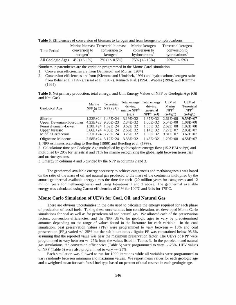
Table 5. Efficiencies of conversion of biomass to kerogen and from kerogen to hydrocarbons.

Time Period

Marine biomass

conversion to

kerogen1.

Terrestrial biomass

conversion to

kerogen1.

Marine kerogen

conversion to

hydrocarbons2.

Terrestrial kerogen

conversion to

hydrocarbons2.

All Geologic Ages 4% (+/- 1%) 2% (+/- 0.5%) 75% (+/- 15%) 20% (+/- 5%)

Numbers in parentheses are the variation programmed in the Monte Carol simulation.

1. Conversion efficiencies are from Demaison and Murris (1984)

2. Conversion efficiencies are from (Klemme and Ulmishek, 1991) and hydrocarbons/kerogen ratios

from Behar et al. (1997), Tissot et al. (1987), Kenneth et al. (1994), Waples (1994), and Klemme

(1994).

Table 6. Net primary production, total emergy, and Unit Emergy Values of NPP by Geologic Age (Oil

and Nat. Gas).

Geological Age

Marine

NPP (g C) 1.

Terrestrial

NPP (g C) 1.

Total emergy

driving

marine NPP2.

(seJ)

Total emergy

driving

terrestrial

NPP2. (seJ)

UEV of

Marine

NPP3.

(seJ/gC)

UEV of

Terrestrial

NPP3.

(seJ/gC)

Silurian 1.23E+24 1.43E+24 3.19E+32 1.37E+32 2.61E+08 9.59E+07 Upper Devonian-Touronian 4.23E+23 9.30E+23 2.34E+32 1.00E+32 5.54E+08 1.08E+08 Pennsylvanian -Lower

Permian

1.38E+24 1.52E+24 3.62E+32 1.55E+32 2.62E+08 1.02E+08 Upper Jurassic 3.66E+24 4.03E+24 2.66E+32 1.14E+32 7.27E+07 2.83E+07 Middle Cretaceous 3.31E+24 3.79E+24 3.25E+32 1.39E+32 9.81E+07 3.67E+07

Oligocene-Miocene 2.58E+24 3.12E+24 3.33E+32 1.43E+32 1.29E+08 4.58E+07

1. NPP estimates according to Beerling (1999) and Beerling et al. (1999).

2. Calculation: time per Geologic Age multiplied by geobiosphere emergy flow (15.2 E24 seJ/yr) and

multiplied by 29% for terrestrial and 71% for marine recognizing the global split between terrestrial

and marine systems.

3. Emergy in columns 4 and 5 divided by the NPP in columns 2 and 3.

The geothermal available energy necessary to achieve catagenesis and methanogenesis was based

on the ratio of the mass of oil and natural gas produced to the mass of the continents multiplied by the

annual geothermal available energy times the time for each (20 million years for catagenesis and 12

million years for methanogenesis) and using Equations 1 and 2 above. The geothermal available

energy was calculated using Carnot efficiencies of 21% for 100oC and 34% for 175

oC.

Monte Carlo Simulation of UEVs for Coal, Oil, and Natural Gas

There are obvious uncertainties in the data used to calculate the emergy required for each phase

of production of fossil fuels. Taking these uncertainties into consideration, we developed Monte Carlo

simulations for coal as well as for petroleum oil and natural gas. We allowed each of the preservation

factors, conversion efficiencies, and the NPP UEVs for geologic ages to vary by predetermined

amounts depending on the range of values found in the literature for each variable. In the coal

simulation, peat preservation values (PF1) were programmed to vary between+/- 15% and coal

preservation (PF2) varied +/- 25% but the sub-bituminous / lignite PF was constrained below 95.6%

assuming that the reported value was near the maximum preservation factor. The UEVs of NPP were

programmed to vary between +/- 25% from the values listed in Tables 3. In the petroleum and natural

gas simulations, the conversion efficiencies (Table 5) were programmed to vary +/-25%. UEV values

of NPP (Table 6) were also programmed to vary +/- 25%

Each simulation was allowed to run for 1000 iterations while all variables were programmed to

vary randomly between minimum and maximum values. We report mean values for each geologic age

and a weighted mean for each fossil fuel type based on percent of total reserve in each geologic age.

547

5.00E+04

7.00E+04

9.00E+04

1.10E+05

1.30E+05

1.50E+05

0 20 40 60 80 100 120 140 160 180 200

Iteration

Tran

sfo

rm

ity (

seJ/J)

A nthrac ite & Bituminous

Sub-bituminous & Lignite

Mean A nthrac ite & Bituminous

Mean Sub-Bituminous & LigniteMean = 9.71E+04 +/- 0.79E+04 seJ/J

Mean = 6.63E+04 +/- 0.51E+04 seJ/J

Figure 3. Results of the Monte Carlo simulation for the transformity of anthracite and bituminous

coal (top) and sub-bituminous & lignite coal (bottom). The gray bands on either side of the mean

represent one standard deviation about the mean.

1.00E+05

1.20E+05

1.40E+05

1.60E+05

1.80E+05

2.00E+05

0 20 40 60 80 100 120 140 160 180 200

Iteration

Tran

sfo

rm

ity (

seJ/J)

Oil

Mean Oil

Nat Gas

Mean Nat Gas

Mean = 1.48E+05 +/- 0.07E+05 seJ/J

Mean = 1.70E+05 +/- 0.06E+05 seJ/J

Figure 4. Results of the Monte Carlo simulation for the transformity of Natural Gas (top) and crude

oil (bottom). The gray bands on either side of the mean represent one standard deviation about the

mean.

548

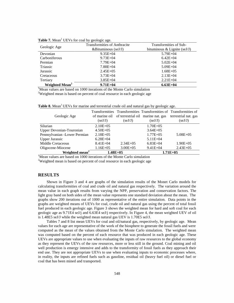
Table 7. Mean1 UEVs for coal by geologic age.

Geologic Age Transformities of Anthracite

&Bituminous (seJ/J)

Transformities of Sub-

bituminous & Lignite (seJ/J)

Devonian 9.35E+04 5.79E+04 Carboniferous 9.73E+04 6.42E+04

Permian 7.79E+04 5.02E+04

Triassic 7.88E+04 5.09E+04

Jurassic 2.45E+05 1.68E+05

Cretaceous 3.73E+04 2.13E+04

Tertiary 3.85E+04 2.21E+04

Weighted Mean2 9.71E+04 6.63E+04

1Mean values are based on 1000 iterations of the Monte Carlo simulation

2Weighted mean is based on percent of coal resource in each geologic age

Table 8. Mean1 UEVs for marine and terrestrial crude oil and natural gas by geologic age.

Geologic Age

Transformities

of marine oil

(seJ/J)

Transformities

of terrestrial oil

(seJ/J)

Transformities of

marine nat. gas

(seJ/J)

Transformities of

terrestrial nat. gas

(seJ/J)

Silurian 2.10E+05 1.70E+05 Upper Devonian-Touronian 4.50E+05 3.64E+05

Pennsylvanian -Lower Permian 2.18E+05 1.77E+05 5.08E+05

Upper Jurassic 6.28E+04 5.11E+04

Middle Cretaceous 8.41E+04 2.34E+05 6.83E+04 1.90E+05

Oligocene-Miocene 1.16E+05 3.00E+05 9.41E+04 2.43E+05

Weighted mean2 1.48E+05 1.71E+05

1Mean values are based on 1000 iterations of the Monte Carlo simulation

2Weighted mean is based on percent of coal resource in each geologic age

RESULTS

Shown in Figure 3 and 4 are graphs of the simulation results of the Monet Carlo models for

calculating transformities of coal and crude oil and natural gas respectively. The variation around the

mean value in each graph results from varying the NPP, preservation and conservation factors. The

light gray band on both sides of the mean value represents one standard deviation about the mean. The

graphs show 200 iterations out of 1000 as representative of the entire simulation. Data points in the

graphs are weighted means of UEVs for coal, crude oil and natural gas using the percent of total fossil

fuel produced in each geologic age. Figure 3 shows the weighted mean for hard and soft coal for each

geologic age as 9.71E4 seJ/j and 6.63E4 seJ/j respectively. In Figure 4, the mean weighted UEV of oil

is 1.48E5 seJ/J while the weighted mean natural gas UEV is 1.70E5 seJ/J.

Tables 7 and 8 list mean UEVs for coal and oil/natural gas, respectively, by geologic age. Mean

values for each age are representative of the work of the biosphere to generate the fossil fuels and were

computed as the mean of the values obtained from the Monte Carlo simulation. The weighted mean

was computed based on the percent of each resource that was produced in each geologic age. These

UEVs are appropriate values to use when evaluating the inputs of raw resources to the global economy

as they represent the UEVs of the raw resources, more or less still in the ground. Coal mining and oil

well production is emergy intensive and adds to the transformity of fossil fuels as they approach their

end use. They are not appropriate UEVs to use when evaluating inputs to economic processes where,

in reality, the inputs are refined fuels such as gasoline, residual oil (heavy fuel oil) or diesel fuel or

coal that has been mined and transported.

549

End Use UEVs

The UEVs computed for the coal, oil, and natural gas resource are UEVs of the geologic resource

and do not include mining, production and transportation. A UEV for the final consumption of these

fossil energies should include all the emergy required to produce them. In the following sections we

compute UEVs for fossil fuels that include mining, production, and transportation.

UEV for Extracted &Transported Fossil Fuels

Table 9 lists the emergy costs of extraction (mining and well drilling, etc) and transportation of

the fossil fuels. The final column is the transformity for coal, oil and natural gas, at the gate prior to

either burning (coal & natural gas) or refining (oil). The computed transformities for coal are

significantly larger than the raw resources while natural gas and oil have lower extraction and

transportation costs. The transformities for soft and hard coal are 68% and 36% higher respectively

than the resource transformity, while those for oil and natural gas are 6% and 4% higher. These higher

transformities are due to mining and transport of the coal resource, and refining of the oil resource.

UEVs for End Use of Petroleum Fuels

Fuels used in machines and transportation are refined petroleum products and thus have higher

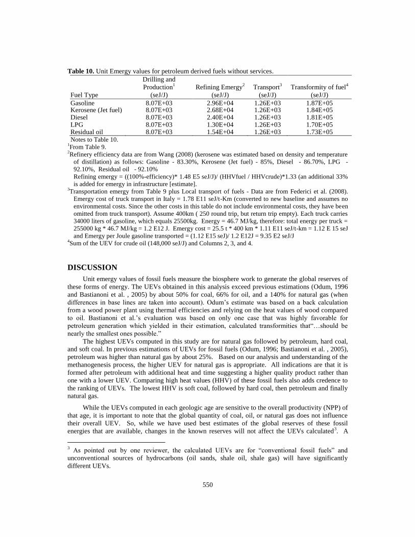
UEVs than the crude petroleum UEVs. Table 10 lists the UEVs for refined petroleum products. Using

data from Argon National Laboratory, USA (Wang, 2008), we computed the UEVs for fuel types

given in Table10 based on refinery efficiencies. The refining process on average adds about nearly

30% to the emergy costs of transportation fuels (gasoline, jet fuel, and diesel) while only about 15% to

LPG and residual oil.

Table 9. Fuel transformities including production and transport costs.

Fuel Type

Mining/Drilling1

(seJ/J)

Transport-12

(seJ/J)

Resource Trasnformity3

(seJ/J)

Soft Coal 1.54E+04 2.97E+04 1.11E+05

Hard Coal 1.23E+04 2.23E+04 1.32E+05

Oil (crude) 8.07E+03 2.48E+02 1.56E+05

Natural Gas 8.07E+03 -- 1.78E+05 1Coal mining- Emergy used in coal mining derived from an LCA by Sagisaka (1999). Total emergy = 2.95

E14 seJ/t of clean coal.

Energy in hard coal = 2.4E10 MJ/t

Energy in soft coal = 1.8E10 MJ/t

Oil and Natural Gas Production- Exploration, drilling and production data from a report by Life Cycle

Associates (2009). Total energy = 4.1% of oil production, therefore 4.1% of UEV for oil = 0.041*1.48E5

seJ/J = 6.07 E4 seJ/J. Added 33% to account for emergy of machinery = 6.1 E4 * 1.33= 8.07 E4 2Rail transport of coal - Data taken from Federici et al. (2008). Emergy cost of rail transport in Italy = 5.35

E11 seJ/t-Km (converted to new baseline and assumes no environmental costs. Since the other costs in

this table do not include environmental costs, they have been omitted from rail transport). Assume

1000km.

Emergy per J transported- Soft Coal = (5.35E11 seJ/t-Km*1000km)/1.8 E10 MJ/t = 2.97 E4 seJ/J

Emergy per J transported- Hard Coal = (5.35E11 seJ/t-Km*1000km)/2.4 E10 MJ/t = 2.23 E4 seJ/J

Oil transport via tanker - Data are from Life Cycle Associates (2009). Estimate of GHG emissions

from transport of oil = 1.0g/MJ of oil transported = 0.3 g oil = 1.26kJ/MJ.

Emergy per J transported oil = (1.26 E3 J * 1.48 E5 seJ/J) / 1E6 J = 1.86 E2 seJ/J. Assume 33% for

emergy of infrastructure. Therefore total emergy per J transported = 1.86 E3 seJ/J * 1.33 = 2.48 E4 3Sum of columns 2 & 3 and the following raw resource transformities:

Soft coal = 6.63 E4 seJ/J Hard coal = 9.71 E4 seJ/j

Oil = 1.48 E5 seJ/J Natural gas = 1.71 E5 seJ/J

550

Table 10. Unit Emergy values for petroleum derived fuels without services.

Fuel Type

Drilling and

Production1

(seJ/J)

Refining Emergy2

(seJ/J)

Transport3

(seJ/J)

Transformity of fuel4

(seJ/J)

Gasoline 8.07E+03 2.96E+04 1.26E+03 1.87E+05 Kerosene (Jet fuel) 8.07E+03 2.68E+04 1.26E+03 1.84E+05 Diesel 8.07E+03 2.40E+04 1.26E+03 1.81E+05 LPG 8.07E+03 1.30E+04 1.26E+03 1.70E+05 Residual oil 8.07E+03 1.54E+04 1.26E+03 1.73E+05 Notes to Table 10.

1From Table 9.

2Refinery efficiency data are from Wang (2008) (kerosene was estimated based on density and temperature

of distillation) as follows: Gasoline - 83.30%, Kerosene (Jet fuel) - 85%, Diesel - 86.70%, LPG -

92.10%, Residual oil - 92.10%

Refining emergy = ((100%-efficiency)* 1.48 E5 seJ/J)/ (HHVfuel / HHVcrude)*1.33 (an additional 33%

is added for emergy in infrastructure [estimate]. 3Transportation emergy from Table 9 plus Local transport of fuels - Data are from Federici et al. (2008).

Emergy cost of truck transport in Italy = 1.78 E11 seJ/t-Km (converted to new baseline and assumes no

environmental costs. Since the other costs in this table do not include environmental costs, they have been

omitted from truck transport). Assume 400km ( 250 round trip, but return trip empty). Each truck carries

34000 liters of gasoline, which equals 25500kg. Energy = 46.7 MJ/kg, therefore: total energy per truck =

255000 kg * 46.7 MJ/kg = 1.2 E12 J. Emergy cost = 25.5 t * 400 km * 1.11 E11 seJ/t-km = 1.12 E 15 seJ

and Emergy per Joule gasoline transported = (1.12 E15 seJ)/ 1.2 E12J = 9.35 E2 seJ/J 4Sum of the UEV for crude oil (148,000 seJ/J) and Columns 2, 3, and 4.

DISCUSSION

Unit emergy values of fossil fuels measure the biosphere work to generate the global reserves of

these forms of energy. The UEVs obtained in this analysis exceed previous estimations (Odum, 1996

and Bastianoni et al. , 2005) by about 50% for coal, 66% for oil, and a 140% for natural gas (when

differences in base lines are taken into account). Odum’s estimate was based on a back calculation

from a wood power plant using thermal efficiencies and relying on the heat values of wood compared

to oil. Bastianoni et al.’s evaluation was based on only one case that was highly favorable for

petroleum generation which yielded in their estimation, calculated transformities that―…should be

nearly the smallest ones possible.‖

The highest UEVs computed in this study are for natural gas followed by petroleum, hard coal,

and soft coal. In previous estimations of UEVs for fossil fuels (Odum, 1996; Bastianoni et al. , 2005),

petroleum was higher than natural gas by about 25%. Based on our analysis and understanding of the

methanogenesis process, the higher UEV for natural gas is appropriate. All indications are that it is

formed after petroleum with additional heat and time suggesting a higher quality product rather than

one with a lower UEV. Comparing high heat values (HHV) of these fossil fuels also adds credence to

the ranking of UEVs. The lowest HHV is soft coal, followed by hard coal, then petroleum and finally

natural gas.

While the UEVs computed in each geologic age are sensitive to the overall productivity (NPP) of

that age, it is important to note that the global quantity of coal, oil, or natural gas does not influence

their overall UEV. So, while we have used best estimates of the global reserves of these fossil

energies that are available, changes in the known reserves will not affect the UEVs calculated3. A

3 As pointed out by one reviewer, the calculated UEVs are for ―conventional fossil fuels‖ and

unconventional sources of hydrocarbons (oil sands, shale oil, shale gas) will have significantly

different UEVs.

551

better understanding of the processes of diagenesis, catagenesis and methanogenesis as well as the

preservation factors from organic matter to kerogen would sharpen the analysis and more than likely

reduce the standard deviation of our simulation results, but would not substantially alter the final

UEVs calculated.

This analysis represents a major departure from previous evaluations of fossil fuel as our results

suggest that they are significantly more valuable (higher transformities) than previously computed

UEVs would support. Since fossil fuels are primary drivers of all economic processes, changes in the

UEVs of this order of magnitude represent a significant change that will require much recalculation of

standard UEVs of many secondary products and processes. It would be convenient if a simple ratio

could be used to transform UEVs of products and processes that were calculated using earlier fossil

fuel UEVs, but unfortunately since every process and product contains differing amounts of fossil

energies in relation to other inputs, there is no simple solution.

Applying Fossil Fuel UEVs

We have provided several UEVs in this paper for each of the fossil fuels. Each is appropriate

under different conditions. When determining the inputs to national economies it will be important to

separate crude oil from refined fuels and oils and applying the appropriate transformity. Coal inputs to

a national economy, if mined within the country should carry the resource transformity (Table 7),

while imported coal should carry the transformity of coal after mining and transport (Table 9). If oil or

natural gas are obtained from resources within the country, use the transformity in Table 8, but if

imported, use the transformities in Tables 9 or 10 depending on fuel type.

We have computed UEVs for fossil resources and fuels without services. UEVs without services

are based solely on the emergy content and the emergy costs of production, transportation, and

refining. Labor is not included. A UEV with services can easily be computed at any stage of the

energy supply chain by multiplying the average price of each resource or fuel type by the emergy

money ratio for the economy of interest. Using average price data from the USA over the first 6

months of 2010, the UEVs of fuels would increase between 20% and 30%. Since the service inputs

are highly dependent on the price of fuel, we leave the addition of the emergy in services to the

individuals using these UEVs for evaluations in other places and at other times.

SUMMARY

A major criticism of the emergy synthesis methodology in the past has been that a single

transformity for oil or coal, for example, was applied worldwide despite the fact that it is well known

that fossil fuels have been developed under wide ranging conditions at very different time scales, and

thus a single transformity is an over simplification. There was no question in our minds that this

critique was accurate and it has taken a number of years to assemble the data (and the time) to re-

evaluate these previous attempts of computing fossil energy transformities.

We have therefore carefully computed UEVs for the fossil fuels based on geologic process and

time scales. We have strengthened our evaluation by taking into consideration the uncertainties that

exist in the general understanding of coal and petroleum genesis through Monte Carlo simulations that

incorporate uncertainty and nonlinearity of the interactions of time, temperature, biology and geology.

We provide new mean UEVs of the coal resource over the entire geologic past range between 6.63 E4

(+/-0.51 E4) seJ/J and 9.71 E4 (+/-0.79 E4) seJ/J. Oil and natural gas resource UEVs have mean

values of 1.48 E5 (+/- 0.07 E5) seJ/J and 1.71 E5 (+/- 0.06 E5) seJ/J respectively. These UEVs

quantify the effort of the geobiosphere in producing these resources and through such quantification

provide a complementary point of view to the usual economic value.

Within the framework of the emergy synthesis method the quality and importance of these fossil

energy resources has been revealed. Some resources are more important than others since they drive

entire chains of processes, and fossil fuels in many respects, occupy a particularly central position in

modern economies. Fossil fuels are a primary energy source and as such the estimation of their

552

production costs by nature and their refining costs by humans is crucial to understanding their value to

society, at least until fossil fuels are no longer the dominant source of energy.

We understand that even this more refined evaluation of a very complex paleogeochemical

system cannot ignore the huge uncertainties that still exist. We look forward to further refinement, as

these uncertainties are decreased through additional research.

REFERENCES

Bastianoni, S, D Campbell, L Susani and E Tiezzi. 2005. The solar transformity of oil and petroleum

natural gas. Ecological Modelling 186, Nr. 2: 212-220. doi:10.1016/j.ecolmodel.2005.01.015

Beerling, D.J. 1999, Quantitative estimates of change in marine and terrestrial primary productivity

over the past 300 million years. Proceedings: Biological Sciences, Royal Society, London. Vol.

266;1821-1827.

Beerling, D.J. 2002. CO2 and the end-Triassic mass extinction. Nature. Vol 415:386-87.

Beerling, D.J., F.I. Woodward, and P.J. Valdes, 1999. Global terrestrial productivity in the mid-

Cretaceous (100 Ma): Model simulations and data. in Barrera, E. and C.C. Johnson (eds).

Evolution of the Cretaceous ocean-climate system, Geological Society of America, Special

Papers, 332, p. 385-390

Behar, F. M. Vandenbroucke, Y. Tang, F. Marquis and J. Espitalie 1997. Thermal cracking of kerogen

in open and close systems: determination of kinetic parameters and stoichiometric coefficients

for oil and gas generation. Organic Geochemisty. Vol. 26, No. 5/6, pp.312-339

Bestougeff, M.A. 1980. Summary of mondial coal resources and reserves: Geographic and geologic

repartition: Revue Inst. Francais Petrole, V.35, p.353-366.

Bois, C. Bouche, P. and Pelet, R. 1982. Global geologic history and distribution of hydrocarbon

reserves: Am. Assoc. Petroleum Geologists Bull., v.66, p.1248-1270.

Brown, M.T. and S. Ulgiati. 1997. Emergy Based Indices and Ratios to Evaluate Sustainability:

Monitoring technology and economies toward environmentally sound innovation. Ecological

Engineering 9:51-69

Brown, M.T. and S. Ulgiati. 2004. Emergy and environmental accounting. In C. Cleveland. (ed)

Encyclopedia of Energy. Elsevier. New York

Brown, M.T. and S. Ulgiati, 2004. Energy quality, emergy, and transformity: H.T. Odum’s

contributions to quantifying and understanding systems. Ecological Modeling. Vol 78;1&2

pp201-213

Chen, G. (2006). Scarcity of exergy and ecological evaluation based on embodied exergy.

Communications in Nonlinear Science and Numerical Simulation, 11(4), 531-552. doi:

10.1016/j.cnsns.2004.11.009.

Cook, E, 1976, Limits to Exploitation of Nonrenewable Resources. Science, 191 (4228), pp 677-682.

Demaison, G., and Murris, R. J.eds., 1984. Petroleum Geochemistry and Basin Evaluation. AAPG

Memoir 35.

Dukes, J. S. (2003). Burning Buried Sunshine : Human Consumption Of Ancient Solar Energy.

Climatic Change, 61, 31-44.

EIA, 2010. U.S. Coal Consumption by End Use Sector, by Census Division and State. US Energy

Information Agency. Downloaded on 21July, 2010 from

http://www.eia.doe.gov/cneaf/coal/page/acr/table26.html.

Field, C.B., M.J. Behrenfeld, J.T. Randerson, and P. Falkowski. 1989 Primary Production of the

Biosphere: Integrating Terrestrial and Oceanic Components. Science 281, 237-40

Federici, M., Ulgiati, S., and Basosi, R., 2008. A thermodynamic, environmental and material flow

analysis of the Italian highway and railway transport systems. Energy_The International Journal,

33: 760–775.

Frolking, S., Roulet, N.T., Tuittila, E., Bubier, J.L., Quillet, A., Talbot, J., and Richard, P. J. H., 2002.

A new model of Holocene peatland net primary production, decomposition, water balance, and

553

peat accumulation. Earth Syst. Dynam. Discuss., 1: 115–167. www.earth-syst-dynam-

discuss.net/1/115/2010/doi:10.5194/esdd-1-115-2010

International Heat Flow Data Base, 2010. Accessed 19 March 2010 http://www.geophysik.rwth-

aachen.de/IHFC/heatflow.html

Kenneth et al., Applied source rock geochemistry. In: The petroleum system - from source to trap

(Edited by L. B. Magoon and W.G. Dow). AAPG Memoir 60, 1994, pp. 93-121. Klemme, H.D. 1994. Petroleum system of the world involving upper Jurassic source rocks, . in

Magoon, L. B, and W. G. Dow (eds.), The petroleum system—from source to trap: Am. Assoc.

Petroleum Geologists Special Volumes M 60: 93-121

Klemme, H.D. and G. F. Ulmishek, 1991. Effective Petroleum Source Rocks of the World:

Stratigraphic Distribution and Controlling Depositional Factors. AAPG Bulletin vol. 75, No. 12:

1809-1851.

Life Cycle Associates. 2009. Assessment of Direct and Indirect GHG Emissions Associated with

Petroleum Fuels. Life Cycle Associates Report LCA-6004-3P. 2009. Prepared for New Fuels

Alliance. Downloaded 22, July 2010 from:

http://www.newfuelsalliance.org/NFA_PImpacts_v35.pdf

Mott, R. A.: 1942, The Origin and Composition of Coals. Fuel in Science and Practice 21, 129–135.

Mott, R. A.: 1943, The Origin and Composition of Coals. Fuel in Science and Practice 22, 20–26.

Odum, H.T. 1988. Self organization, transformity, and information. Science 242(Nov. 25,

1988):1132-1139.

Odum, H.T. 1996. Environmental Accounting: Emergy and environmental decision making. John

Wiley & Sons, New York 370p.

Peters, K.E. and M.R. Cassa. 1994. Applied source rock geochemistry. In Magoon, L. B, and W. G.

Dow (eds.), The petroleum system—from source to trap: Am. Assoc. Petroleum Geologists

Special Volumes M 60: 93-120.

Platt, T. and B. Irwin, 1973. Caloric content of phytoplankton. Limnology and Oceanography.18: 306-

309

Protano, G., and Ulgiati, S., 2010. Emergy study of worldwide biogeochemical formation of fossil

fuels. In Brown, M.T. (ed) Book of Proceedings of the Sixth BIENNIAL EMERGY

EVALUATION and RESEARCH CONFERENCE. January 14 through January 16, 2010,

Gainesville, Florida

Retallack, J.G., Veevers, J.J., and Morante, R., 1996. Global coal gab between Permian-Triassic

extinction and Middle Triassic recovery of peat-forming plants. Geologic Society of America

Bulletin, 108(2): 195-207.

Sagisaka, M. 1999. Lifecycle Environmental Evaluation of Exploitation & CO2 Sequestration of Coal,

Life Cycle Assessment Research Centre, National Institute of Advanced Industrial Science &

Technology (AIST), JAPAN, 1999. Downloaded on July 21, 2010 from

http://www.codata.org/06conf/presentations/B9/B9-Sagisaka.ppt

Szargut, J., A. Ziezbik, W. Stanek. 2002. Depletion of the non-renewable natural exergy resources as

a measure of the ecological cost. Energy Conversion and Management 43:1149–1163

Szargut, J., D. R. Morris and F. R. Steward: Exergy analysis of thermal, chemical and metallurgical

processes. Hemisphere Publishing Corporation. New York, 400 p.

Teichmuller, R. and M. Teichmuller. 1986. Relations Between Coalification And Palaeogeothermics

In Variscan And Alpidic Foredeeps Of Western Europe. Paleogeothermics 5: 53–78.

http://www.springerlink.com/index/W2V4216P7U36H4Q1.pdf.

Tissot B.P., R. Pelet, and P. Ungerer. 1987. Thermal history of sedimentary basins, maturation

indices, and kinetics of oil and gas generation. Am. Assoc. Petroleum Geologists Bulletin 71:12,

p. 1445-1466.

Tissot, B.P and D.H. Welte. 1984. Petroleum Formation and Occurrence. Springer-Verlag. New York.

699p.

Veizer, J., and S. L. Jansen. 1985. Basement and Sedimentary Recycling--2: Time Dimension to

554

Global Tectonics. Journal of Geology, 93:625-643.

Veizer, J. , P. Laznicka, and S.L.Jansen. 1989. Mineralization through geologic time: recycling

perspective. American Journal of Science 289:4. Pp 484-524

Walker, S., 2000. Major Coalfields of the World. IEA Coal Research, London. pp.131.

Wang, M. (2008). Estimation of Energy Efficiencies of U.S. Petroleum Refineries. Fuel. Retrieved on

20 July, 2010 from

http://www.transportation.anl.gov/modeling_simulation/GREET/pdfs/energy_eff_petroleum_refi

neries-03-08.pdf.

Waples, D. W. 1994. Maturity modeling: thermal indicators, hydrocarbon generation, and oil cracking.

in Magoon, L. B, and W. G. Dow (eds.), The petroleum system—from source to trap: Am.

Assoc. Petroleum Geologists Special Volumes M 60:285-306

Ward, C., 1984. Coal Geology and Coal Technology Blackwell Scientific Press, 1984.