Embed Size (px)
Citation preview
Emerging Biofuels: Outlook of Effects on U.S. Grain, Oilseed, and Livestock Markets
Simla Tokgoz, Amani Elobeid, Jacinto Fabiosa, Dermot J. Hayes, Bruce A. Babcock, Tun-Hsiang (Edward) Yu, Fengxia Dong,
Chad E. Hart, and John C. Beghin
Staff Report 07-SR 101 May 2007
Center for Agricultural and Rural Development Iowa State University
Ames, Iowa 50011-1070 www.card.iastate.edu
The authors are with the Center for Agricultural and Rural Development at Iowa State University. Support for this research came from a grant from USDA and the following organizations: National Grain and Feed Association, American Meat Institute, Grocery Manufacturers Association/Food Products Association, National Cattlemen’s Beef Association, National Chicken Council, National Pork Producers Council, National Oilseed Processors Association, National Turkey Federation, and the North American Millers Association.
The authors are with the Center for Agricultural and Rural Development at Iowa State University. This paper is available online on the CARD Web site: www.card.iastate.edu. Permission is granted to excerpt or quote this information with appropriate attribution to the authors and to CARD. Questions or comments about the contents of this paper should be directed to Bruce Babcock, 578 Heady Hall, Iowa State University, Ames, IA 50011-1070; Ph: (515) 294-6785; Fax: (515) 293-6336; E-mail: [email protected]. The U.S. Department of Agriculture (USDA) prohibits discrimination in all its programs and activities on the basis of race, color, national origin, gender, religion, age, disability, political beliefs, sexual orientation, and marital or family status. (Not all prohibited bases apply to all programs.) Persons with disabilities who require alternative means for communication of program information (Braille, large print, audiotape, etc.) should contact USDA’s TARGET Center at (202) 720-2600 (voice and TDD). To file a complaint of discrimination, write USDA, Director, Office of Civil Rights, Room 326-W, Whitten Building, 14th and Independence Avenue, SW, Washington, DC 20250-9410 or call (202) 720-5964 (voice and TDD). USDA is an equal opportunity provider and employer. Iowa State University does not discriminate on the basis of race, color, age, religion, national origin, sexual orientation, gender identity, sex, marital status, disability, or status as a U.S. veteran. Inquiries can be directed to the Director of Equal Opportunity and Diversity, 3680 Beardshear Hall, (515) 294-7612.
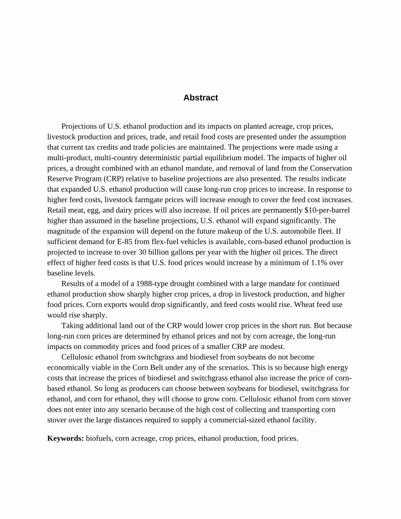
Abstract Projections of U.S. ethanol production and its impacts on planted acreage, crop prices, livestock production and prices, trade, and retail food costs are presented under the assumption that current tax credits and trade policies are maintained. The projections were made using a multi-product, multi-country deterministic partial equilibrium model. The impacts of higher oil prices, a drought combined with an ethanol mandate, and removal of land from the Conservation Reserve Program (CRP) relative to baseline projections are also presented. The results indicate that expanded U.S. ethanol production will cause long-run crop prices to increase. In response to higher feed costs, livestock farmgate prices will increase enough to cover the feed cost increases. Retail meat, egg, and dairy prices will also increase. If oil prices are permanently $10-per-barrel higher than assumed in the baseline projections, U.S. ethanol will expand significantly. The magnitude of the expansion will depend on the future makeup of the U.S. automobile fleet. If sufficient demand for E-85 from flex-fuel vehicles is available, corn-based ethanol production is projected to increase to over 30 billion gallons per year with the higher oil prices. The direct effect of higher feed costs is that U.S. food prices would increase by a minimum of 1.1% over baseline levels. Results of a model of a 1988-type drought combined with a large mandate for continued ethanol production show sharply higher crop prices, a drop in livestock production, and higher food prices. Corn exports would drop significantly, and feed costs would rise. Wheat feed use would rise sharply. Taking additional land out of the CRP would lower crop prices in the short run. But because long-run corn prices are determined by ethanol prices and not by corn acreage, the long-run impacts on commodity prices and food prices of a smaller CRP are modest. Cellulosic ethanol from switchgrass and biodiesel from soybeans do not become economically viable in the Corn Belt under any of the scenarios. This is so because high energy costs that increase the prices of biodiesel and switchgrass ethanol also increase the price of corn-based ethanol. So long as producers can choose between soybeans for biodiesel, switchgrass for ethanol, and corn for ethanol, they will choose to grow corn. Cellulosic ethanol from corn stover does not enter into any scenario because of the high cost of collecting and transporting corn stover over the large distances required to supply a commercial-sized ethanol facility. Keywords: biofuels, corn acreage, crop prices, ethanol production, food prices.
3 / CARD Staff Report
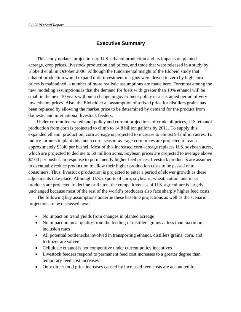
Executive Summary This study updates projections of U.S. ethanol production and its impacts on planted acreage, crop prices, livestock production and prices, and trade that were released in a study by Elobeid et al. in October 2006. Although the fundamental insight of the Elobeid study that ethanol production would expand until investment margins were driven to zero by high corn prices is maintained, a number of more realistic assumptions are made here. Foremost among the new modeling assumptions is that the demand for fuels with greater than 10% ethanol will be small in the next 10 years without a change in government policy or a sustained period of very low ethanol prices. Also, the Elobeid et al. assumption of a fixed price for distillers grains has been replaced by allowing the market price to be determined by demand for the product from domestic and international livestock feeders. Under current federal ethanol policy and current projections of crude oil prices, U.S. ethanol production from corn is projected to climb to 14.8 billion gallons by 2011. To supply this expanded ethanol production, corn acreage is projected to increase to almost 94 million acres. To induce farmers to plant this much corn, season-average corn prices are projected to reach approximately $3.40 per bushel. Most of this increased corn acreage replaces U.S. soybean acres, which are projected to decline to 69 million acres. Soybean prices are projected to average above $7.00 per bushel. In response to permanently higher feed prices, livestock producers are assumed to eventually reduce production to allow their higher production costs to be passed onto consumers. Thus, livestock production is projected to enter a period of slower growth as these adjustments take place. Although U.S. exports of corn, soybeans, wheat, cotton, and meat products are projected to decline or flatten, the competitiveness of U.S. agriculture is largely unchanged because most of the rest of the world’s producers also face sharply higher feed costs. The following key assumptions underlie these baseline projections as well as the scenario projections to be discussed next:
• No impact on trend yields from changes in planted acreage • No impact on meat quality from the feeding of distillers grains at less than maximum
inclusion rates • All potential bottlenecks involved in transporting ethanol, distillers grains, corn, and
fertilizer are solved • Cellulosic ethanol is not competitive under current policy incentives • Livestock feeders respond to permanent feed cost increases to a greater degree than
temporary feed cost increases • Only direct food price increases caused by increased feed costs are accounted for
Emerging Biofuels: Outlook of Effects / 4
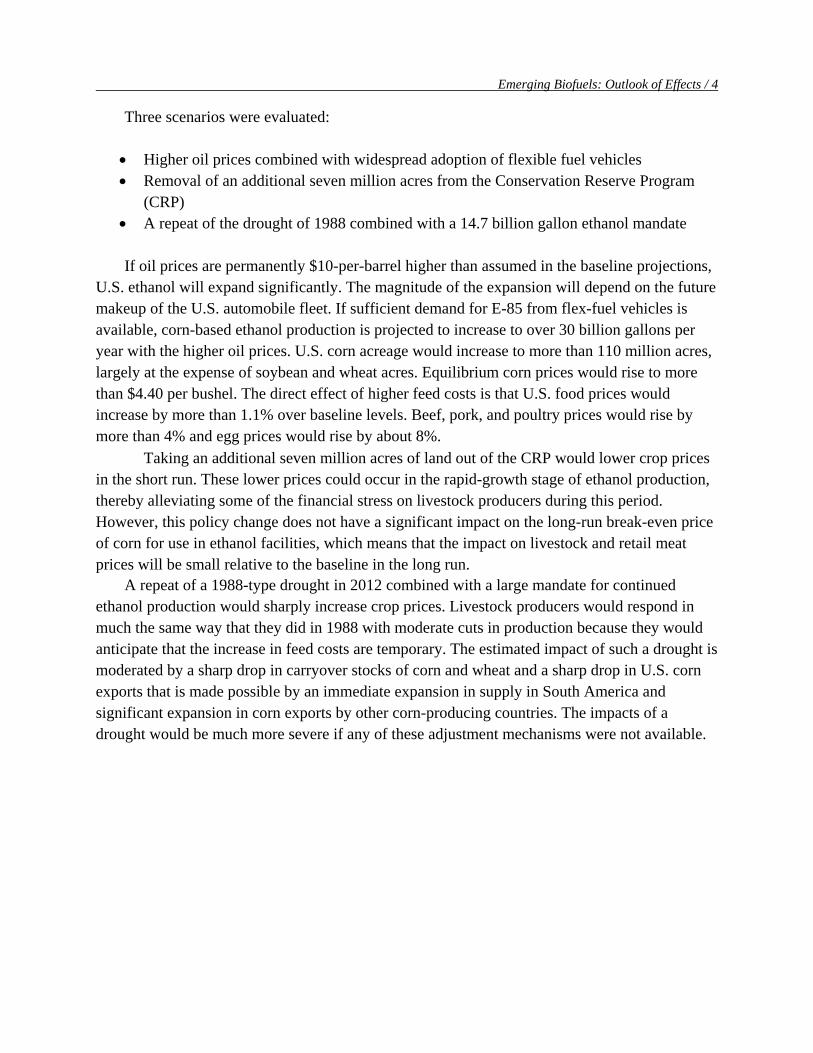
Three scenarios were evaluated:
• Higher oil prices combined with widespread adoption of flexible fuel vehicles • Removal of an additional seven million acres from the Conservation Reserve Program
(CRP) • A repeat of the drought of 1988 combined with a 14.7 billion gallon ethanol mandate
If oil prices are permanently $10-per-barrel higher than assumed in the baseline projections, U.S. ethanol will expand significantly. The magnitude of the expansion will depend on the future makeup of the U.S. automobile fleet. If sufficient demand for E-85 from flex-fuel vehicles is available, corn-based ethanol production is projected to increase to over 30 billion gallons per year with the higher oil prices. U.S. corn acreage would increase to more than 110 million acres, largely at the expense of soybean and wheat acres. Equilibrium corn prices would rise to more than $4.40 per bushel. The direct effect of higher feed costs is that U.S. food prices would increase by more than 1.1% over baseline levels. Beef, pork, and poultry prices would rise by more than 4% and egg prices would rise by about 8%.
Taking an additional seven million acres of land out of the CRP would lower crop prices in the short run. These lower prices could occur in the rapid-growth stage of ethanol production, thereby alleviating some of the financial stress on livestock producers during this period. However, this policy change does not have a significant impact on the long-run break-even price of corn for use in ethanol facilities, which means that the impact on livestock and retail meat prices will be small relative to the baseline in the long run. A repeat of a 1988-type drought in 2012 combined with a large mandate for continued ethanol production would sharply increase crop prices. Livestock producers would respond in much the same way that they did in 1988 with moderate cuts in production because they would anticipate that the increase in feed costs are temporary. The estimated impact of such a drought is moderated by a sharp drop in carryover stocks of corn and wheat and a sharp drop in U.S. corn exports that is made possible by an immediate expansion in supply in South America and significant expansion in corn exports by other corn-producing countries. The impacts of a drought would be much more severe if any of these adjustment mechanisms were not available.
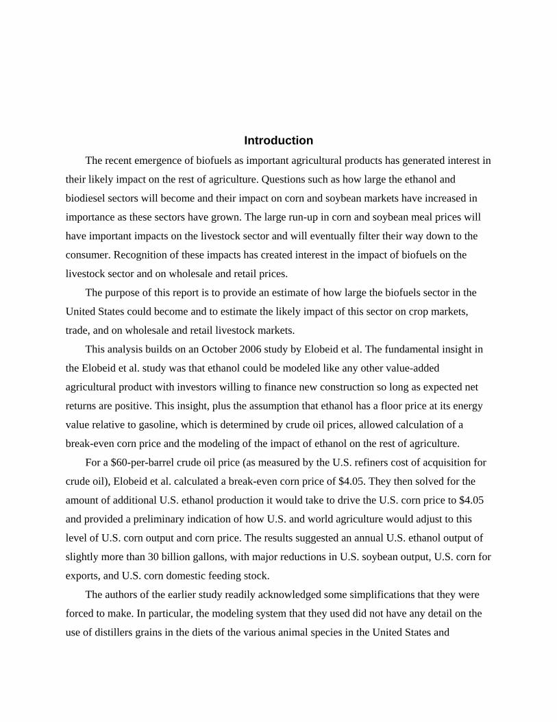
Introduction The recent emergence of biofuels as important agricultural products has generated interest in
their likely impact on the rest of agriculture. Questions such as how large the ethanol and
biodiesel sectors will become and their impact on corn and soybean markets have increased in
importance as these sectors have grown. The large run-up in corn and soybean meal prices will
have important impacts on the livestock sector and will eventually filter their way down to the
consumer. Recognition of these impacts has created interest in the impact of biofuels on the
livestock sector and on wholesale and retail prices.
The purpose of this report is to provide an estimate of how large the biofuels sector in the
United States could become and to estimate the likely impact of this sector on crop markets,
trade, and on wholesale and retail livestock markets.
This analysis builds on an October 2006 study by Elobeid et al. The fundamental insight in
the Elobeid et al. study was that ethanol could be modeled like any other value-added
agricultural product with investors willing to finance new construction so long as expected net
returns are positive. This insight, plus the assumption that ethanol has a floor price at its energy
value relative to gasoline, which is determined by crude oil prices, allowed calculation of a
break-even corn price and the modeling of the impact of ethanol on the rest of agriculture.
For a $60-per-barrel crude oil price (as measured by the U.S. refiners cost of acquisition for
crude oil), Elobeid et al. calculated a break-even corn price of $4.05. They then solved for the
amount of additional U.S. ethanol production it would take to drive the U.S. corn price to $4.05
and provided a preliminary indication of how U.S. and world agriculture would adjust to this
level of U.S. corn output and corn price. The results suggested an annual U.S. ethanol output of
slightly more than 30 billion gallons, with major reductions in U.S. soybean output, U.S. corn for
exports, and U.S. corn domestic feeding stock.
The authors of the earlier study readily acknowledged some simplifications that they were
forced to make. In particular, the modeling system that they used did not have any detail on the
use of distillers grains in the diets of the various animal species in the United States and
Emerging Biofuels: Outlook of Effects / 2
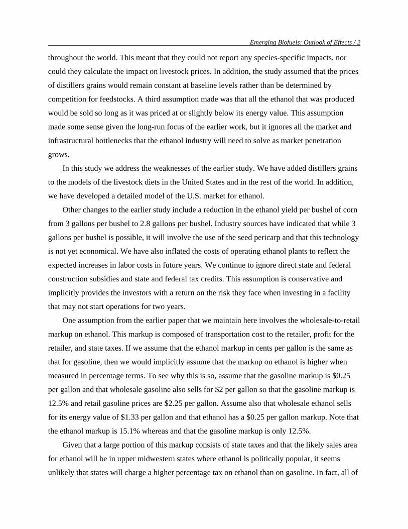
throughout the world. This meant that they could not report any species-specific impacts, nor
could they calculate the impact on livestock prices. In addition, the study assumed that the prices
of distillers grains would remain constant at baseline levels rather than be determined by
competition for feedstocks. A third assumption made was that all the ethanol that was produced
would be sold so long as it was priced at or slightly below its energy value. This assumption
made some sense given the long-run focus of the earlier work, but it ignores all the market and
infrastructural bottlenecks that the ethanol industry will need to solve as market penetration
grows.
In this study we address the weaknesses of the earlier study. We have added distillers grains
to the models of the livestock diets in the United States and in the rest of the world. In addition,
we have developed a detailed model of the U.S. market for ethanol.
Other changes to the earlier study include a reduction in the ethanol yield per bushel of corn
from 3 gallons per bushel to 2.8 gallons per bushel. Industry sources have indicated that while 3
gallons per bushel is possible, it will involve the use of the seed pericarp and that this technology
is not yet economical. We have also inflated the costs of operating ethanol plants to reflect the
expected increases in labor costs in future years. We continue to ignore direct state and federal
construction subsidies and state and federal tax credits. This assumption is conservative and
implicitly provides the investors with a return on the risk they face when investing in a facility
that may not start operations for two years.
One assumption from the earlier paper that we maintain here involves the wholesale-to-retail
markup on ethanol. This markup is composed of transportation cost to the retailer, profit for the
retailer, and state taxes. If we assume that the ethanol markup in cents per gallon is the same as
that for gasoline, then we would implicitly assume that the markup on ethanol is higher when
measured in percentage terms. To see why this is so, assume that the gasoline markup is $0.25
per gallon and that wholesale gasoline also sells for $2 per gallon so that the gasoline markup is
12.5% and retail gasoline prices are $2.25 per gallon. Assume also that wholesale ethanol sells
for its energy value of $1.33 per gallon and that ethanol has a $0.25 per gallon markup. Note that
the ethanol markup is 15.1% whereas and that the gasoline markup is only 12.5%.
Given that a large portion of this markup consists of state taxes and that the likely sales area
for ethanol will be in upper midwestern states where ethanol is politically popular, it seems
unlikely that states will charge a higher percentage tax on ethanol than on gasoline. In fact, all of
3 / CARD Staff Report
the states that have visited the issue so far have actually worked to impose lower per-gallon taxes
on ethanol than on gasoline.1 Therefore, we have assumed that the wholesale-to-retail markup on
ethanol is the same in percentage terms as the markup on gasoline. The continued use of this
assumption means that if ethanol sells at its energy value at retail pumps then it will also be
priced at its energy value at the wholesale level.
As mentioned earlier, the Elobeid et al. study did not include any species-specific analysis of
livestock. One problem that we encountered when we included livestock was how to project the
impact of a dramatic increase in feed prices on livestock supply. The models that we use project
behavior by assuming that market participants will respond in the future as they have in the past.
For example, in the summer of 1995, U.S. corn prices went up dramatically because parts of the
country were experiencing a temporary scarcity. Livestock growers could see a healthy corn crop
in the fields and they could observe a futures market that predicted a low price after this crop was
harvested. As a result, many livestock producers chose to ignore the short-term losses that they
were experiencing and stay in business. We would not expect to see this kind of behavior in
response to a permanent increase in feed prices but we do not have any historical evidence to
base this on because we have not experienced a feed cost increase that livestock producers
viewed as being permanent.
Defining Long-Run Equilibrium As was true for the Elobeid et al. study, we use the concept of a long-run equilibrium to help
us understand the eventual impact of the biofuels sector on agriculture. This concept is very 1 States that have chosen to impose differential taxes on ethanol and gasoline (source: http://www.fhwa.dot.gov/ohim/mmfr/jul06/trmfuel.htm): Iowa—Effective 07/01/02, motor fuel tax rates will be adjusted annually based on the amounts of ethanol-blended gasoline being sold and distributed annually. Minnesota—There is a credit to the wholesaler of 15¢ per gallon of alcohol used to make gasohol. Montana—There is an alcohol distiller credit of 30¢ per gallon of alcohol produced in the state with state agricultural products and used to make gasohol. Nebraska—Rates are variable, adjusted quarterly. The gasoline and gasohol include 0.6¢ per gallon. New Nebraska ethanol production facilities may receive an ethanol production credit equal to 18¢ per gallon of ethanol used to fuel motor vehicles. North Dakota—There is a producer credit of 40¢ per gallon of agriculturally derived alcohol produced in the state and used to make gasohol. Ohio—Dealers are refunded 10¢ per gallon of each qualified fuel (ethanol or methanol) blended with unleaded gasoline. South Dakota—There is a credit at the rate of the gasoline tax to distributors blending gasoline with ethanol to product gasohol. There is also a producer incentive payment of 20¢ per gallon.
Emerging Biofuels: Outlook of Effects / 4
intuitive. When we are at a long-run equilibrium, no group of producers or consumers has an
incentive to change its behavior. For example, if the ethanol industry is in equilibrium, then there
is no incentive to build new ethanol plants and there is no incentive to shut down existing plants.
In response to increased demand for corn by the ethanol sector, feed prices increase and stay
high for several years. We constrained the models to follow economic theory that shows that
increased costs will lead to a reduction in supply and to a price increase so that net returns are
once again at levels sufficient to keep livestock producers in business. This constraint was
imposed on our baseline projections as well as on our analysis of various scenarios. This
assumption forces the adjustment to ethanol by the livestock sector onto the wholesale and
export markets and eventually to the retail consumer. It takes time for this adjustment to occur.
We refer to model results that fully reflect these adjustments as the “long-run equilibrium.”
We imposed full price transmission of higher feed costs to Canada and Mexico, as well as to
other countries where we expect this to occur. We did not impose full feed price transmission in
other countries, such as the European Union and its feed wheat market, where trade barriers
exist. The effect of this assumption was that the United States does not lose a significant amount
of competitive advantage in international meat markets when U.S. corn and soybean meal prices
increase. High U.S. feed prices cause high international feed prices, and the U.S. meat industry
continues to have a cost advantage in meat production. If we were to run the model without this
assumption, most of the adjustment of the livestock sector would be achieved through dramatic
reductions in net exports, a result that assumes that the rest of the world somehow gains a
competitive edge over U.S. livestock producers.
Differences between Results of the Two Studies The report by Elobeid et al. was widely read, and it seems likely that many readers of this
report will be familiar with the earlier report’s results. Therefore, it is worthwhile to summarize
the key differences in the results. These are driven in large part by the inclusion of distillers
grains (DG) in this study and by the model of ethanol demand that we now use.
Impact of the Inclusion of Distillers Grains on the Results In the earlier work, a rapid increase in production of DG caused a reduction in soybean meal
prices and a reduction in soybean prices. In the new model we find that DG enter the rations of
5 / CARD Staff Report
ruminant animals, and that they replace corn mostly and soybean meal only to a limited extent.
With a large U.S. and international market for DG in ruminants, the DG price reflects its feed
value in ruminant rations as a replacement for corn. This means that DG prices will track corn
prices. Poultry and pork rations initially respond to a surplus of DG with relatively high inclusion
rates, but as markets adjust and as DG prices rise, these species eventually revert to a corn-
soybean meal diet.
The inclusion of DG in the model produces some profound and somewhat counterintuitive
effects. For example, we had originally assumed that the impact of the ethanol boom would be
lower for beef producers than for hog and poultry producers because DG can more readily be
included in ruminant rations that in hog and poultry rations. Instead, because DG prices track
corn prices, the impact on cattle feed is as great as the impact on hog feed.
With more expensive DG, world poultry and swine producers continue to purchase corn and
soybean meal and thus soybean prices increase rather than decrease. This increase in soybean
prices causes South American soybean acres to increase substantially as the United States
reduces its soybean production. In Elobeid et al., South America turned from soybean production
to corn production, and by the end of the period the United States was importing a small amount
of corn. In this report, the United States continues to export corn because South America
concentrates on soybean production.
Impact of Adding an Ethanol Demand Component to the Model As mentioned earlier, Elobeid et al. simply assumed that the U.S. ethanol industry could sell
all of its production on the U.S. market at its retail energy value. Because the amount of ethanol
that was projected to be produced was much greater than that needed for a nationwide E-10
blend, this meant that as much as 50% of the ethanol was projected to be consumed via E-85
blends.
When we added an ethanol demand component to this study, we included a careful analysis
of the number and location of existing and new flex-fuel vehicles (FFVs). We also made the
number of FFVs responsive to the price of ethanol relative to its energy value. This analysis
showed that the projected number of FFVs in key midwestern states (where ethanol would be
cheapest relative to gasoline) was insufficient to consume the projected 30 billion gallons of
ethanol.
Emerging Biofuels: Outlook of Effects / 6
There is a chicken-and-egg problem with E-85. It will only pay for gas stations to install E-
85 tanks and pumps and for consumers to purchase FFVs or convert existing cars to run on E-85
if ethanol sells at a significant discount to gasoline. But if ethanol sells at such a discount it does
not pay to build new ethanol plants. We refer to this problem as the “E-85 bottleneck,” and we
include this bottleneck in our baseline results.
Note that the E-85 bottleneck results are in equilibrium in that it is not in the interests of any
party to change their behavior. Gas stations do not see any reason to add E-85 pumps and most
consumers do not see any reason to buy E-85 cars. The ethanol sector expands until it has driven
the price of ethanol below its energy value relative to gasoline and then it stops expanding. At
the end of the projection period the ethanol sector breaks even. Corn prices gradually fall back to
reflect the lack of new ethanol facilities coupled with increased corn yields.
A second impact of adding ethanol demand to the model is that once the plants that are
currently under construction are completed, we can then use the model to understand ethanol
supply decisions. We assume that this occurs in 2010, at which time we model possible future
plant construction by looking at an investor who is considering an investment in a new ethanol
plant.
One factor that we do not account for in this study is the possibility that expanded ethanol
production will impact the price of gasoline. If ethanol captures a significant share of the U.S.
fuel supply, it may begin to affect oil refiners’ margins and their subsequent decisions about
which products to produce and the prices of those products.
Methodology As was true for the earlier paper by Elobeid et al., we use a very broad model of the world
agricultural economy to evaluate the likely impact of biofuels growth on agricultural markets.
The system that we use is a customized version of the deterministic Food and Agricultural Policy
Research Institute (FAPRI) modeling system that contains models of supply and demand for all
important, temperate agricultural products in all relevant counties.
For any crude oil price we calculate the price of unleaded gasoline. This price, along with
the capacity of the ethanol industry, determines the price of ethanol (adjusted for the blender’s
credit) and the incentive to invest in additional ethanol production capacity. Ethanol production
determines the demand for corn. Investment in new ethanol plants will take place if the market
7 / CARD Staff Report
price of corn allows a prospective plant to cover all the costs of owning and operating an ethanol
plant. Long-run equilibrium prices for ethanol, crops, and livestock are achieved when there is
no incentive to construct new plants, no incentive to expand or contract livestock production, and
all crop markets clear.
We are aware of only one set of commodity models that have the required multi-commodity,
international coverage to allow all of the various interactions that are needed for this study.
These models are developed and operated by FAPRI analysts. We have customized these models
to examine how world agriculture will respond to the set of prices that will cause the agricultural
energy sector to stabilize.2 Elobeid, Tokgoz, Yu, Dong, and Fabiosa are responsible for
developing and maintaining the FAPRI international models for sweeteners, grains, oilseeds,
dairy, and livestock.3
The Importance of Crude Oil Prices In the Elobeid et al. study, for every $0.10 increase in the market value of ethanol, the break-
even corn prices in our model increase by $0.28.4 This means that relatively small changes in
ethanol prices will have a very large impact on the price of corn and, by extension, on
agriculture. We model ethanol demand based on gasoline prices and ultimately on crude oil
prices. A $0.10 increase in the retail price of gasoline is not unusual, but a $0.28-per-bushel
permanent increase in corn prices is an unusual event and would cause an increase in cash rents
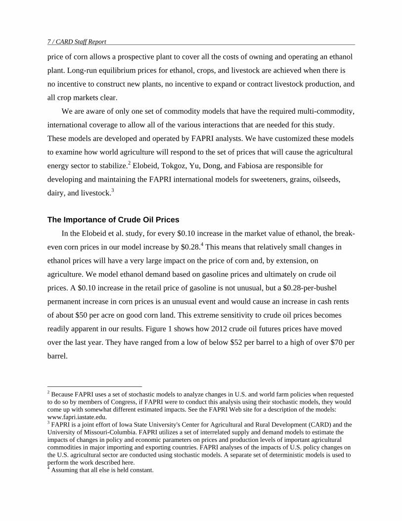
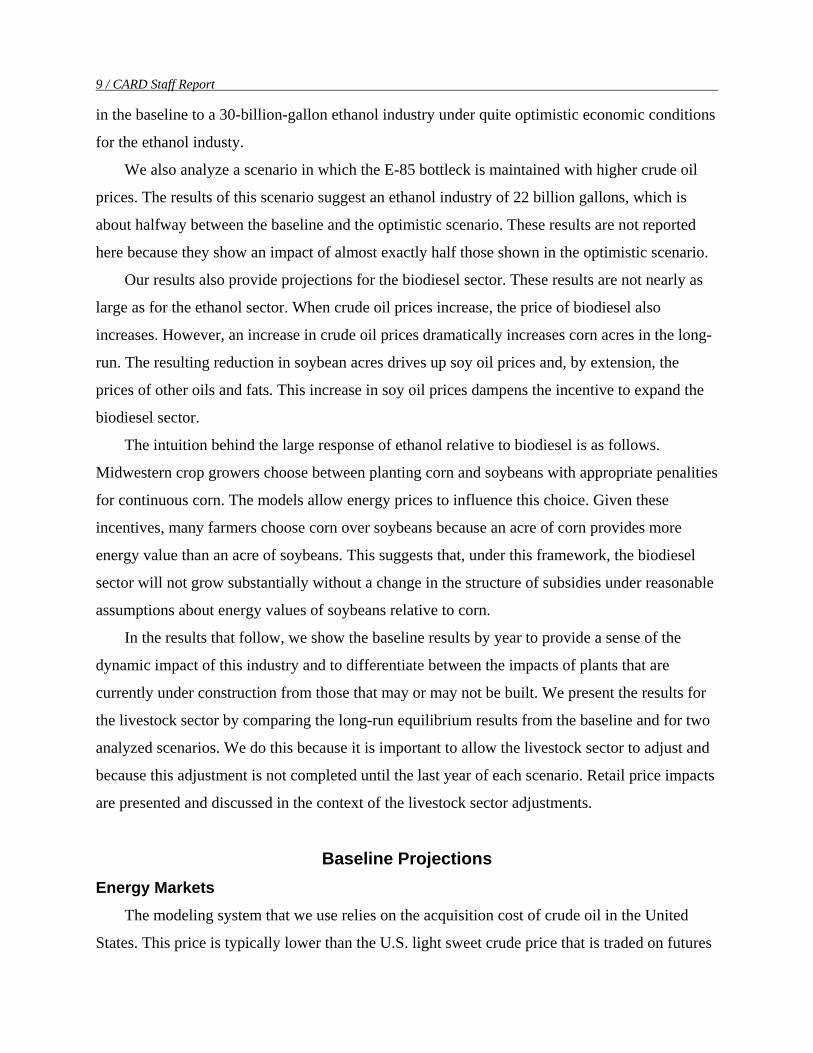
of about $50 per acre on good corn land. This extreme sensitivity to crude oil prices becomes
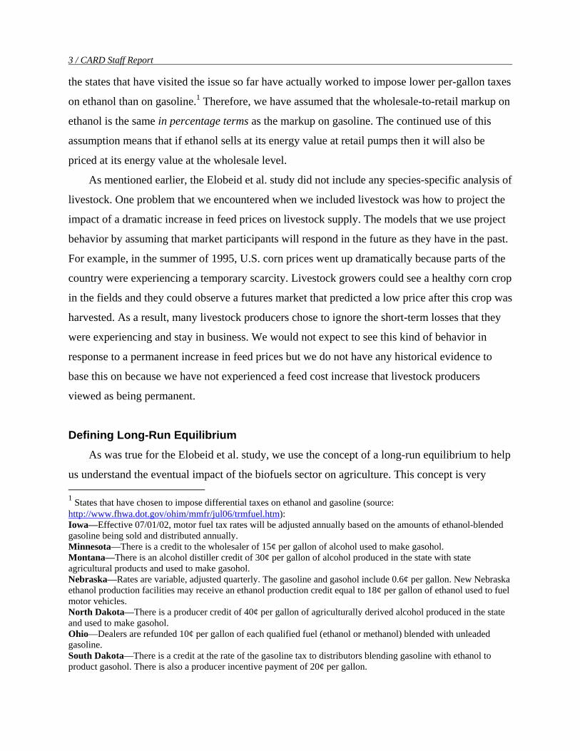
readily apparent in our results. Figure 1 shows how 2012 crude oil futures prices have moved
over the last year. They have ranged from a low of below $52 per barrel to a high of over $70 per
barrel.
2 Because FAPRI uses a set of stochastic models to analyze changes in U.S. and world farm policies when requested to do so by members of Congress, if FAPRI were to conduct this analysis using their stochastic models, they would come up with somewhat different estimated impacts. See the FAPRI Web site for a description of the models: www.fapri.iastate.edu. 3 FAPRI is a joint effort of Iowa State University's Center for Agricultural and Rural Development (CARD) and the University of Missouri-Columbia. FAPRI utilizes a set of interrelated supply and demand models to estimate the impacts of changes in policy and economic parameters on prices and production levels of important agricultural commodities in major importing and exporting countries. FAPRI analyses of the impacts of U.S. policy changes on the U.S. agricultural sector are conducted using stochastic models. A separate set of deterministic models is used to perform the work described here. 4 Assuming that all else is held constant.
Emerging Biofuels: Outlook of Effects / 8
50
55
60
65
70
75
11/21
/2005
12/21
/2005
1/21/2
006
2/21/2
006
3/21/2
006
4/21/2
006
5/21/2
006
6/21/2
006
7/21/2
006
8/21/2
006
9/21/2
006
10/21
/2006
11/21
/2006
12/21
/2006
1/21/2
007
2/21/2
007
3/21/2
007
Date
$ pe
r Bar
rel
FIGURE 1. Weekly closing prices on the NYMEX light sweet crude futures for delivery in December 2012
To demonstrate the impact of an increase in crude oil prices over the level that is used in the
baseline projections, we ran a scenario whereby crude oil prices are $10 higher for each year of
the projection period. As will be shown, this increase in crude oil prices dramatically increases
the investment in ethanol production. Under the assumption that the E-85 barrier is eliminated,
this increase in crude oil prices increases projected ethanol production from corn by 15 billion
gallons.
The equilibrium corn price in the baseline scenario is $3.16 per bushel. The soybean meal
price is $158 per ton. The equilibrium corn price with higher oil prices and without the E-85
barrier is $4.42 per bushel, with a soybean meal price of $193 per ton. These prices suggest a
relatively large difference in animal feed ration prices and therefore provide a good basis against
which to evalute the impact of ethanol on the livestock sector and on retail prices.
Therefore, the discussion of the impact of ethanol on the livestock sector is framed in terms
of the impact of a move from an industry supplying approximately 15 billion gallons of ethanol
9 / CARD Staff Report
in the baseline to a 30-billion-gallon ethanol industry under quite optimistic economic conditions
for the ethanol industy.
We also analyze a scenario in which the E-85 bottleck is maintained with higher crude oil
prices. The results of this scenario suggest an ethanol industry of 22 billion gallons, which is
about halfway between the baseline and the optimistic scenario. These results are not reported
here because they show an impact of almost exactly half those shown in the optimistic scenario.
Our results also provide projections for the biodiesel sector. These results are not nearly as
large as for the ethanol sector. When crude oil prices increase, the price of biodiesel also
increases. However, an increase in crude oil prices dramatically increases corn acres in the long-
run. The resulting reduction in soybean acres drives up soy oil prices and, by extension, the
prices of other oils and fats. This increase in soy oil prices dampens the incentive to expand the
biodiesel sector.
The intuition behind the large response of ethanol relative to biodiesel is as follows.
Midwestern crop growers choose between planting corn and soybeans with appropriate penalities
for continuous corn. The models allow energy prices to influence this choice. Given these
incentives, many farmers choose corn over soybeans because an acre of corn provides more
energy value than an acre of soybeans. This suggests that, under this framework, the biodiesel
sector will not grow substantially without a change in the structure of subsidies under reasonable
assumptions about energy values of soybeans relative to corn.
In the results that follow, we show the baseline results by year to provide a sense of the
dynamic impact of this industry and to differentiate between the impacts of plants that are
currently under construction from those that may or may not be built. We present the results for
the livestock sector by comparing the long-run equilibrium results from the baseline and for two
analyzed scenarios. We do this because it is important to allow the livestock sector to adjust and
because this adjustment is not completed until the last year of each scenario. Retail price impacts
are presented and discussed in the context of the livestock sector adjustments.
Baseline Projections Energy Markets
The modeling system that we use relies on the acquisition cost of crude oil in the United
States. This price is typically lower than the U.S. light sweet crude price that is traded on futures
Emerging Biofuels: Outlook of Effects / 10
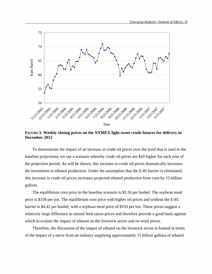
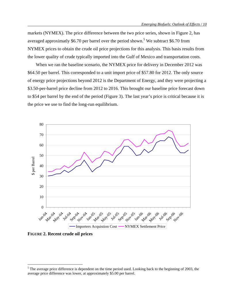
markets (NYMEX). The price difference between the two price series, shown in Figure 2, has
averaged approximatly $6.70 per barrel over the period shown.5 We subtract $6.70 from
NYMEX prices to obtain the crude oil price projections for this analysis. This basis results from
the lower quality of crude typically imported into the Gulf of Mexico and transportation costs.
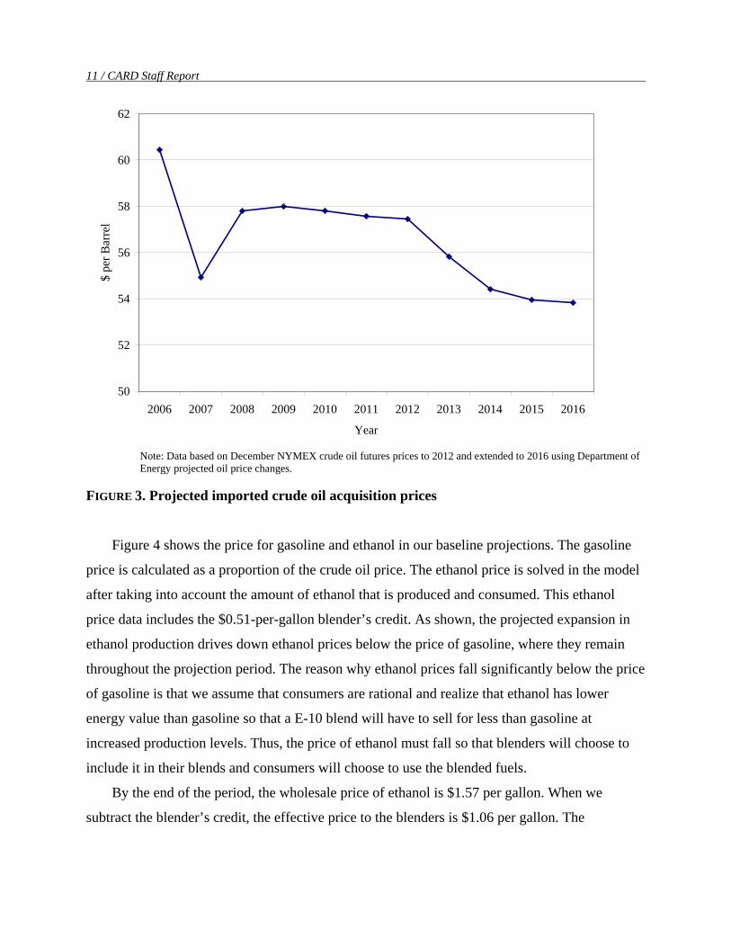
When we ran the baseline scenario, the NYMEX price for delivery in December 2012 was
$64.50 per barrel. This corresponded to a unit import price of $57.80 for 2012. The only source
of energy price projections beyond 2012 is the Department of Energy, and they were projecting a
$3.50-per-barrel price decline from 2012 to 2016. This brought our baseline price forecast down
to $54 per barrel by the end of the period (Figure 3). The last year’s price is critical because it is
the price we use to find the long-run equilibrium.
0
10
20
30
40
50
60
70
80
Jan-04
Mar-04
May-04
Jul-04
Sep-04
Nov-04
Jan-05
Mar-05
May-05
Jul-05
Sep-05
Nov-05
Jan-06
Mar-06
May-06
Jul-06
Sep-06
Nov-06
$ pe
r Bar
rel
Importers Acquistion Cost NYMEX Settlement Price FIGURE 2. Recent crude oil prices
5 The average price difference is dependent on the time period used. Looking back to the beginning of 2003, the average price difference was lower, at approximately $5.00 per barrel.
11 / CARD Staff Report
50
52
54
56
58
60
62
2006 2007 2008 2009 2010 2011 2012 2013 2014 2015 2016
Year
$ pe
r Bar
rel
Note: Data based on December NYMEX crude oil futures prices to 2012 and extended to 2016 using Department of Energy projected oil price changes.
FIGURE 3. Projected imported crude oil acquisition prices
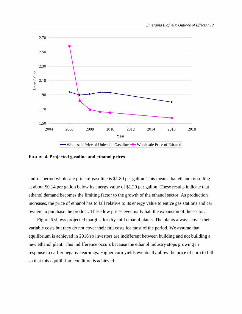
Figure 4 shows the price for gasoline and ethanol in our baseline projections. The gasoline
price is calculated as a proportion of the crude oil price. The ethanol price is solved in the model
after taking into account the amount of ethanol that is produced and consumed. This ethanol
price data includes the $0.51-per-gallon blender’s credit. As shown, the projected expansion in
ethanol production drives down ethanol prices below the price of gasoline, where they remain
throughout the projection period. The reason why ethanol prices fall significantly below the price
of gasoline is that we assume that consumers are rational and realize that ethanol has lower
energy value than gasoline so that a E-10 blend will have to sell for less than gasoline at
increased production levels. Thus, the price of ethanol must fall so that blenders will choose to
include it in their blends and consumers will choose to use the blended fuels.
By the end of the period, the wholesale price of ethanol is $1.57 per gallon. When we
subtract the blender’s credit, the effective price to the blenders is $1.06 per gallon. The
Emerging Biofuels: Outlook of Effects / 12
1.50
1.70
1.90
2.10
2.30
2.50
2.70
2004 2006 2008 2010 2012 2014 2016 2018
Year
$ pe
r Gal
lon
Wholesale Price of Unleaded Gasoline Wholesale Price of Ethanol
FIGURE 4. Projected gasoline and ethanol prices
end-of-period wholesale price of gasoline is $1.80 per gallon. This means that ethanol is selling
at about $0.14 per gallon below its energy value of $1.20 per gallon. These results indicate that
ethanol demand becomes the limiting factor to the growth of the ethanol sector. As production
increases, the price of ethanol has to fall relative to its energy value to entice gas stations and car
owners to purchase the product. These low prices eventually halt the expansion of the sector.
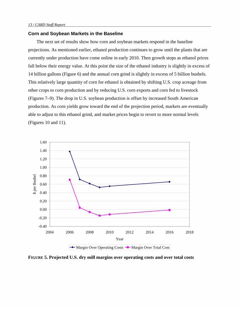
Figure 5 shows projected margins for dry-mill ethanol plants. The plants always cover their
variable costs but they do not cover their full costs for most of the period. We assume that
equilibrium is achieved in 2016 so investors are indifferent between building and not building a
new ethanol plant. This indifference occurs because the ethanol industry stops growing in
response to earlier negative earnings. Higher corn yields eventually allow the price of corn to fall
so that this equilibrium condition is achieved.
13 / CARD Staff Report
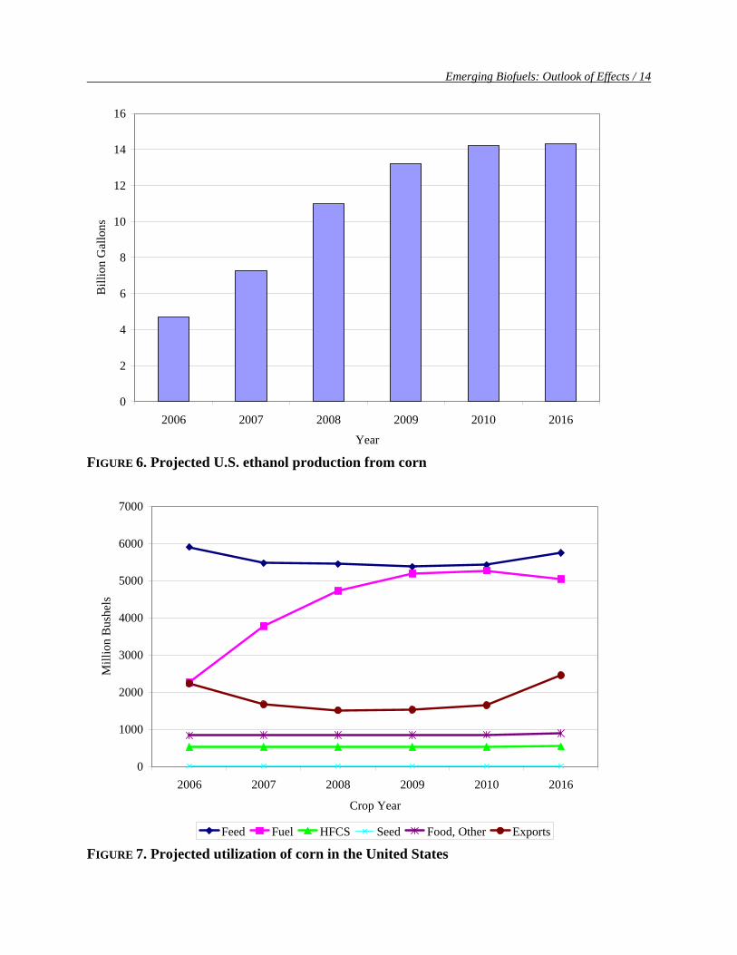
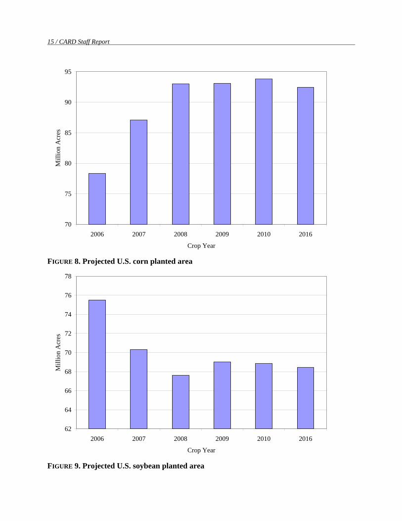
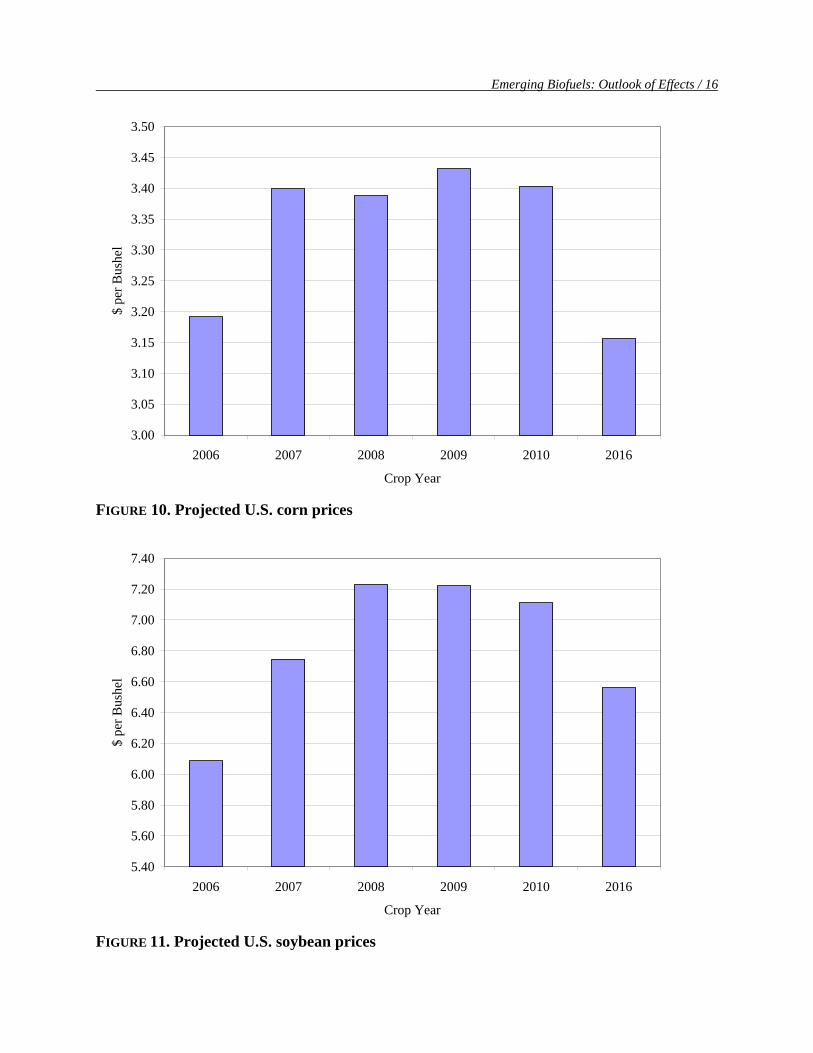
Corn and Soybean Markets in the Baseline The next set of results show how corn and soybean markets respond in the baseline
projections. As mentioned earlier, ethanol production continues to grow until the plants that are
currently under production have come online in early 2010. Then growth stops as ethanol prices
fall below their energy value. At this point the size of the ethanol industry is slightly in excess of
14 billion gallons (Figure 6) and the annual corn grind is slightly in excess of 5 billion bushels.
This relatively large quantity of corn for ethanol is obtained by shifting U.S. crop acreage from
other crops to corn production and by reducing U.S. corn exports and corn fed to livestock
(Figures 7–9). The drop in U.S. soybean production is offset by increased South American
production. As corn yields grow toward the end of the projection period, markets are eventually
able to adjust to this ethanol grind, and market prices begin to revert to more normal levels
(Figures 10 and 11).
-0.40
-0.20
0.00
0.20
0.40
0.60
0.80
1.00
1.20
1.40
1.60
2004 2006 2008 2010 2012 2014 2016 2018
Year
$ pe
r Bus
hel
Margin Over Operating Costs Margin Over Total Cost FIGURE 5. Projected U.S. dry mill margins over operating costs and over total costs
Emerging Biofuels: Outlook of Effects / 14
0
2
4
6
8
10
12
14
16
2006 2007 2008 2009 2010 2016
Year
Bill
ion
Gal
lons
FIGURE 6. Projected U.S. ethanol production from corn
0
1000
2000
3000
4000
5000
6000
7000
2006 2007 2008 2009 2010 2016
Crop Year
Mill
ion
Bus
hels
Feed Fuel HFCS Seed Food, Other Exports FIGURE 7. Projected utilization of corn in the United States
15 / CARD Staff Report
70
75
80
85
90
95
2006 2007 2008 2009 2010 2016
Crop Year
Mill
ion
Acr
es
FIGURE 8. Projected U.S. corn planted area
62
64
66
68
70
72
74
76
78
2006 2007 2008 2009 2010 2016
Crop Year
Mill
ion
Acr
es
FIGURE 9. Projected U.S. soybean planted area
Emerging Biofuels: Outlook of Effects / 16
3.00
3.05
3.10
3.15
3.20
3.25
3.30
3.35
3.40
3.45
3.50
2006 2007 2008 2009 2010 2016
Crop Year
$ pe
r Bus
hel
FIGURE 10. Projected U.S. corn prices
5.40
5.60
5.80
6.00
6.20
6.40
6.60
6.80
7.00
7.20
7.40
2006 2007 2008 2009 2010 2016
Crop Year
$ pe
r Bus
hel
FIGURE 11. Projected U.S. soybean prices
17 / CARD Staff Report
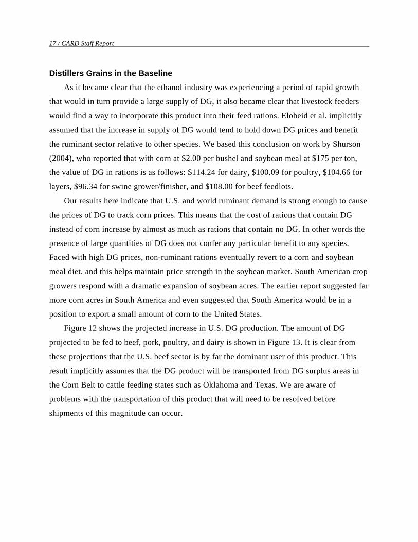
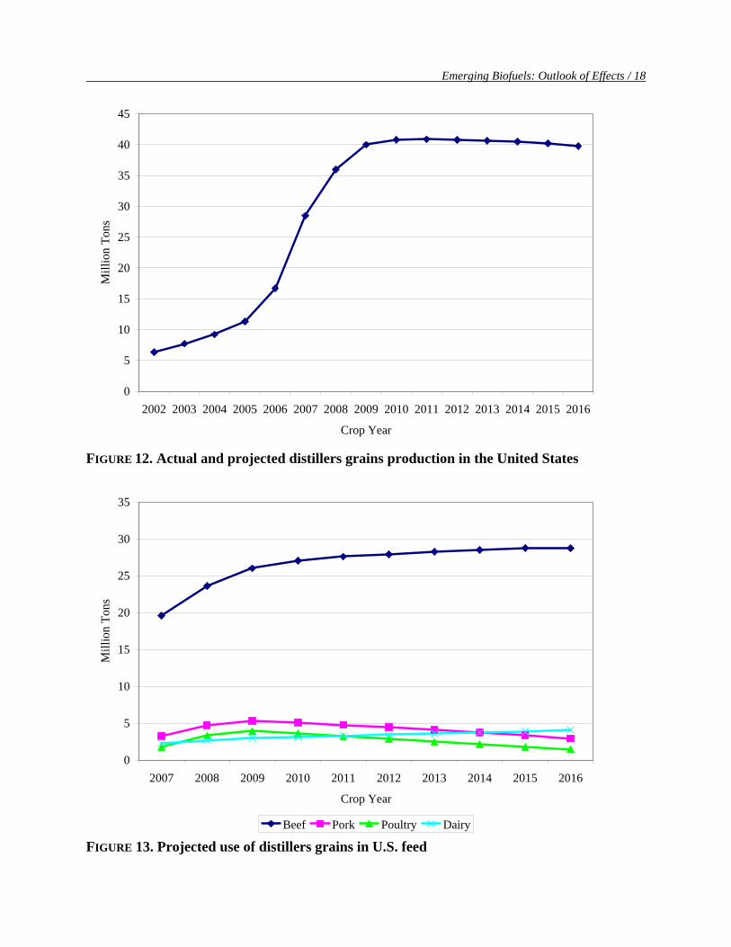
Distillers Grains in the Baseline
As it became clear that the ethanol industry was experiencing a period of rapid growth
that would in turn provide a large supply of DG, it also became clear that livestock feeders
would find a way to incorporate this product into their feed rations. Elobeid et al. implicitly
assumed that the increase in supply of DG would tend to hold down DG prices and benefit
the ruminant sector relative to other species. We based this conclusion on work by Shurson
(2004), who reported that with corn at $2.00 per bushel and soybean meal at $175 per ton,
the value of DG in rations is as follows: $114.24 for dairy, $100.09 for poultry, $104.66 for
layers, $96.34 for swine grower/finisher, and $108.00 for beef feedlots.
Our results here indicate that U.S. and world ruminant demand is strong enough to cause
the prices of DG to track corn prices. This means that the cost of rations that contain DG
instead of corn increase by almost as much as rations that contain no DG. In other words the
presence of large quantities of DG does not confer any particular benefit to any species.
Faced with high DG prices, non-ruminant rations eventually revert to a corn and soybean
meal diet, and this helps maintain price strength in the soybean market. South American crop
growers respond with a dramatic expansion of soybean acres. The earlier report suggested far
more corn acres in South America and even suggested that South America would be in a
position to export a small amount of corn to the United States.
Figure 12 shows the projected increase in U.S. DG production. The amount of DG
projected to be fed to beef, pork, poultry, and dairy is shown in Figure 13. It is clear from
these projections that the U.S. beef sector is by far the dominant user of this product. This
result implicitly assumes that the DG product will be transported from DG surplus areas in
the Corn Belt to cattle feeding states such as Oklahoma and Texas. We are aware of
problems with the transportation of this product that will need to be resolved before
shipments of this magnitude can occur.
Emerging Biofuels: Outlook of Effects / 18
0
5
10
15
20
25
30
35
40
45
2002 2003 2004 2005 2006 2007 2008 2009 2010 2011 2012 2013 2014 2015 2016
Crop Year
Mill
ion
Tons
FIGURE 12. Actual and projected distillers grains production in the United States
0
5
10
15
20
25
30
35
2007 2008 2009 2010 2011 2012 2013 2014 2015 2016
Crop Year
Mill
ion
Tons
Beef Pork Poultry Dairy FIGURE 13. Projected use of distillers grains in U.S. feed
19 / CARD Staff Report
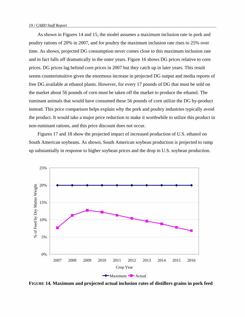
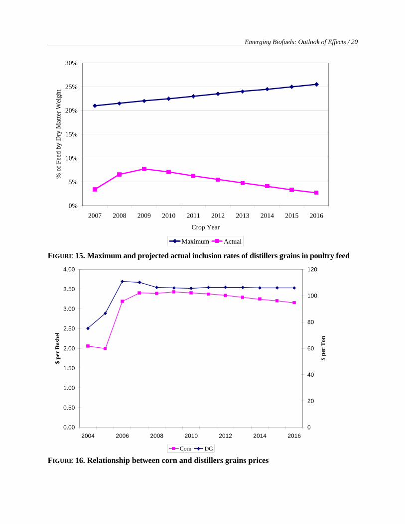
As shown in Figures 14 and 15, the model assumes a maximum inclusion rate in pork and
poultry rations of 20% in 2007, and for poultry the maximum inclusion rate rises to 25% over
time. As shown, projected DG consumption never comes close to this maximum inclusion rate
and in fact falls off dramatically in the outer years. Figure 16 shows DG prices relative to corn
prices. DG prices lag behind corn prices in 2007 but they catch up in later years. This result
seems counterintuitive given the enormous increase in projected DG output and media reports of
free DG available at ethanol plants. However, for every 17 pounds of DG that must be sold on
the market about 56 pounds of corn must be taken off the market to produce the ethanol. The
ruminant animals that would have consumed these 56 pounds of corn utilize the DG by-product
instead. This price comparison helps explain why the pork and poultry industries typically avoid
the product. It would take a major price reduction to make it worthwhile to utilize this product in
non-ruminant rations, and this price discount does not occur.
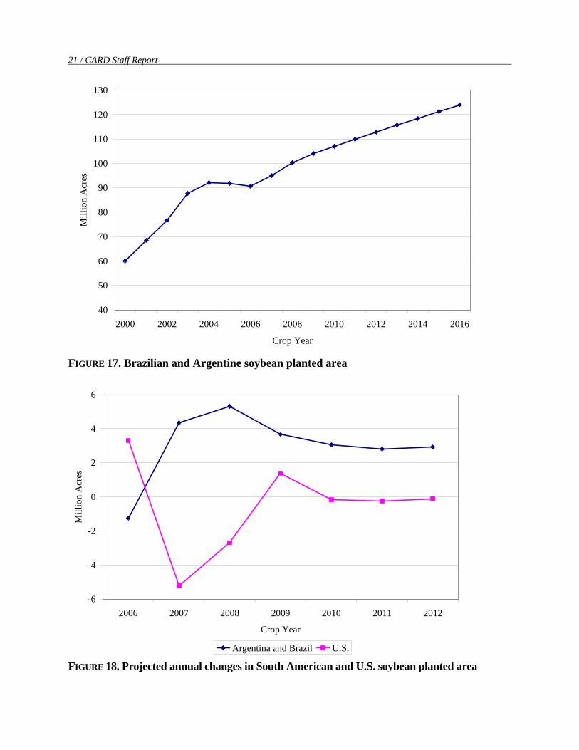
Figures 17 and 18 show the projected impact of increased production of U.S. ethanol on
South American soybeans. As shown, South American soybean production is projected to ramp
up substantially in response to higher soybean prices and the drop in U.S. soybean production.
0%
5%
10%
15%
20%
25%
2007 2008 2009 2010 2011 2012 2013 2014 2015 2016
Crop Year
% o
f Fee
d by
Dry
Mat
ter W
eigh
t
Maximum Actual FIGURE 14. Maximum and projected actual inclusion rates of distillers grains in pork feed
Emerging Biofuels: Outlook of Effects / 20
0%
5%
10%
15%
20%
25%
30%
2007 2008 2009 2010 2011 2012 2013 2014 2015 2016
Crop Year
% o
f Fee
d by
Dry
Mat
ter W
eigh
t
Maximum Actual FIGURE 15. Maximum and projected actual inclusion rates of distillers grains in poultry feed
0.00
0.50
1.00
1.50
2.00
2.50
3.00
3.50
4.00
2004 2006 2008 2010 2012 2014 2016
$ pe
r B
ushe
l
0
20
40
60
80
100
120
$ pe
r T
on
Corn DG FIGURE 16. Relationship between corn and distillers grains prices
21 / CARD Staff Report
40
50
60
70
80
90
100
110
120
130
2000 2002 2004 2006 2008 2010 2012 2014 2016
Crop Year
Mill
ion
Acr
es
FIGURE 17. Brazilian and Argentine soybean planted area
-6
-4
-2
0
2
4
6
2006 2007 2008 2009 2010 2011 2012
Crop Year
Mill
ion
Acr
es
Argentina and Brazil U.S.
FIGURE 18. Projected annual changes in South American and U.S. soybean planted area
Emerging Biofuels: Outlook of Effects / 22
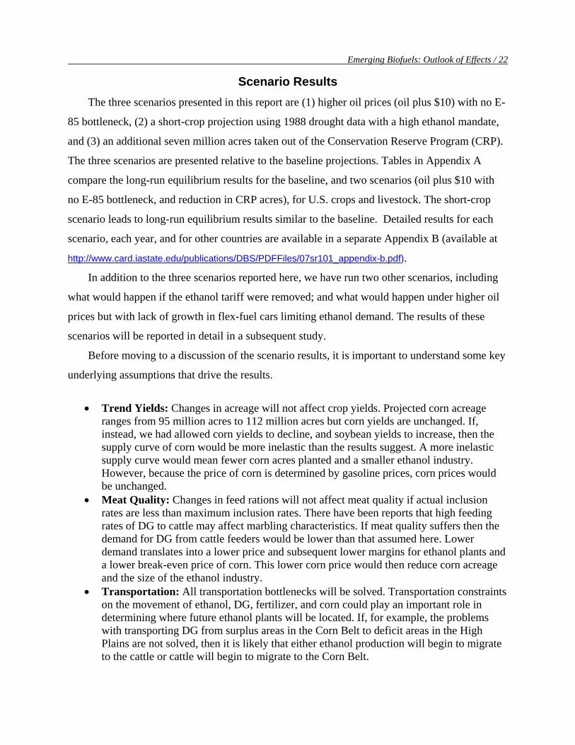
Scenario Results The three scenarios presented in this report are (1) higher oil prices (oil plus $10) with no E-
85 bottleneck, (2) a short-crop projection using 1988 drought data with a high ethanol mandate,
and (3) an additional seven million acres taken out of the Conservation Reserve Program (CRP).
The three scenarios are presented relative to the baseline projections. Tables in Appendix A
compare the long-run equilibrium results for the baseline, and two scenarios (oil plus $10 with
no E-85 bottleneck, and reduction in CRP acres), for U.S. crops and livestock. The short-crop
scenario leads to long-run equilibrium results similar to the baseline. Detailed results for each
scenario, each year, and for other countries are available in a separate Appendix B (available at
http://www.card.iastate.edu/publications/DBS/PDFFiles/07sr101_appendix-b.pdf).
In addition to the three scenarios reported here, we have run two other scenarios, including
what would happen if the ethanol tariff were removed; and what would happen under higher oil
prices but with lack of growth in flex-fuel cars limiting ethanol demand. The results of these
scenarios will be reported in detail in a subsequent study.
Before moving to a discussion of the scenario results, it is important to understand some key
underlying assumptions that drive the results.
• Trend Yields: Changes in acreage will not affect crop yields. Projected corn acreage
ranges from 95 million acres to 112 million acres but corn yields are unchanged. If, instead, we had allowed corn yields to decline, and soybean yields to increase, then the supply curve of corn would be more inelastic than the results suggest. A more inelastic supply curve would mean fewer corn acres planted and a smaller ethanol industry. However, because the price of corn is determined by gasoline prices, corn prices would be unchanged.
• Meat Quality: Changes in feed rations will not affect meat quality if actual inclusion rates are less than maximum inclusion rates. There have been reports that high feeding rates of DG to cattle may affect marbling characteristics. If meat quality suffers then the demand for DG from cattle feeders would be lower than that assumed here. Lower demand translates into a lower price and subsequent lower margins for ethanol plants and a lower break-even price of corn. This lower corn price would then reduce corn acreage and the size of the ethanol industry.
• Transportation: All transportation bottlenecks will be solved. Transportation constraints on the movement of ethanol, DG, fertilizer, and corn could play an important role in determining where future ethanol plants will be located. If, for example, the problems with transporting DG from surplus areas in the Corn Belt to deficit areas in the High Plains are not solved, then it is likely that either ethanol production will begin to migrate to the cattle or cattle will begin to migrate to the Corn Belt.
23 / CARD Staff Report
• Permanent versus Temporary Price Shocks: Crop price increases caused by expansion of ethanol production are assumed to be permanent. Thus, the livestock industry is assumed to adjust production levels to maintain profitability. Crop price increases caused by a short crop are assumed to be temporary so that the livestock industry only makes short-run production adjustments as needed. Thus, the livestock price increases caused by a temporary shock will be lower than those caused by a permanent shock.
• Ethanol from Cellulose: This study only assesses the relative profitability of producing ethanol from corn, corn stover, and switchgrass grown in the Corn Belt. Because ethanol from corn is the only one of these three sources to generate positive returns, it is the only one that we include in our baseline and scenarios. Other sources of ethanol from cellulose may prove more feasible.
• Food Price Limitations: This study only assesses the impacts of ethanol on food prices from the direct effects of higher feed costs on livestock. We do not measure food price increases from high fructose corn sweeteners or the effects on fruit and vegetable supplies from increased competition for land from corn. In addition, food price increases are assumed to be set in perfectly competitive markets. This assumption implies that higher feed prices travel through supply chains in fixed, whole-dollar amounts. If instead higher feed prices move through in fixed percentage terms, then food price increases would be greater than reported here. As such, this study likely understates the actual impact on food prices from ethanol.
The baseline and the oil-plus-$10 scenario probably represent the upper and lower bounds of
the size and impact of ethanol, and therefore the differences across them provide a very clear
indicator of the impact of this industry on other sectors. The ethanol grind in the baseline
scenario is approximately 5 billion bushels, which doubles under higher oil prices. The corn
price in the baseline is $3.16 per bushel, and in the scenario it is $4.43 per bushel.
Note that the total impact of the ethanol industry on livestock is greater than what is reported
in the oil-plus-$10 scenario because the corn price in the baseline is at $3.16, well above the corn
price that was typical before the ethanol boom began. The impacts of taking an additional seven
million acres out of CRP are ultimately smaller than expected. Additional cropland initially
depresses corn prices. Lower corn prices result from additional supplies of corn to provide
feedstock for ethanol plants and livestock feeders. These lower corn prices could occur in the
rapid-growth stage of ethanol production, thereby alleviating some of the financial stress on
livestock producers during this period. However, this policy change does not have a significant
impact on the long-run break-even price of corn for use in ethanol facilities, which means that
the impact on livestock and retail meat prices will be small relative to the baseline.
Results for all the livestock species follow a similar pattern. Feed prices increase
dramatically, as do livestock farmgate prices. For example, an increase in the corn price from
Emerging Biofuels: Outlook of Effects / 24
$3.16 to $4.43 and a $34.23-per-ton increase in the soybean meal price result in an 18.4%
increase in the cost of producing pork and an 18.4% increase in live hog prices. This relatively
large live hog price change leads to a relatively small increase of 4.2% in retail pork prices. The
assumption that we use to set retail prices are that per-unit feed cost increases are passed through
intact through the meat supply chain. Thus, as the ratio of feed cost to total value at each point in
the supply chain decreases, so too does the percent change in price from ethanol. Per capita pork
consumption falls by 2% and pork exports fall by 17%. Total pork production falls by 4.6%. The
impact on the retail price is small because none of the other costs associated with processing,
transporting, and retailing pork is impacted by ethanol. Per capita pork consumption does not
respond very strongly to a retail price increase because the prices of all livestock products
increase by similar amounts at the same time. Pork exports fall because worldwide pork
consumption falls slightly in response to higher pork prices and because the United States loses a
small part of its competitive position relative to the European Union.
Results for beef, poultry, eggs, dairy products, and turkeys all follow similar patterns, as
shown in the tables in Appendix A and Appendix B (provided in a separate document). Overall
retail meat and dairy product prices increase by approximately 5%. Note that if we had included
the full impact of ethanol starting with a $1.90 corn price and increasing to $4.43 with a
proportionate increase in soybean meal prices, then the retail price impact would be
approximately 10%. Again, this impact on retail price levels seems surprisingly small given the
enormous upheavals in the livestock feed sector. But a 10% increase in retail prices for affected
products is a large and unforeseen increase in the cost of living.
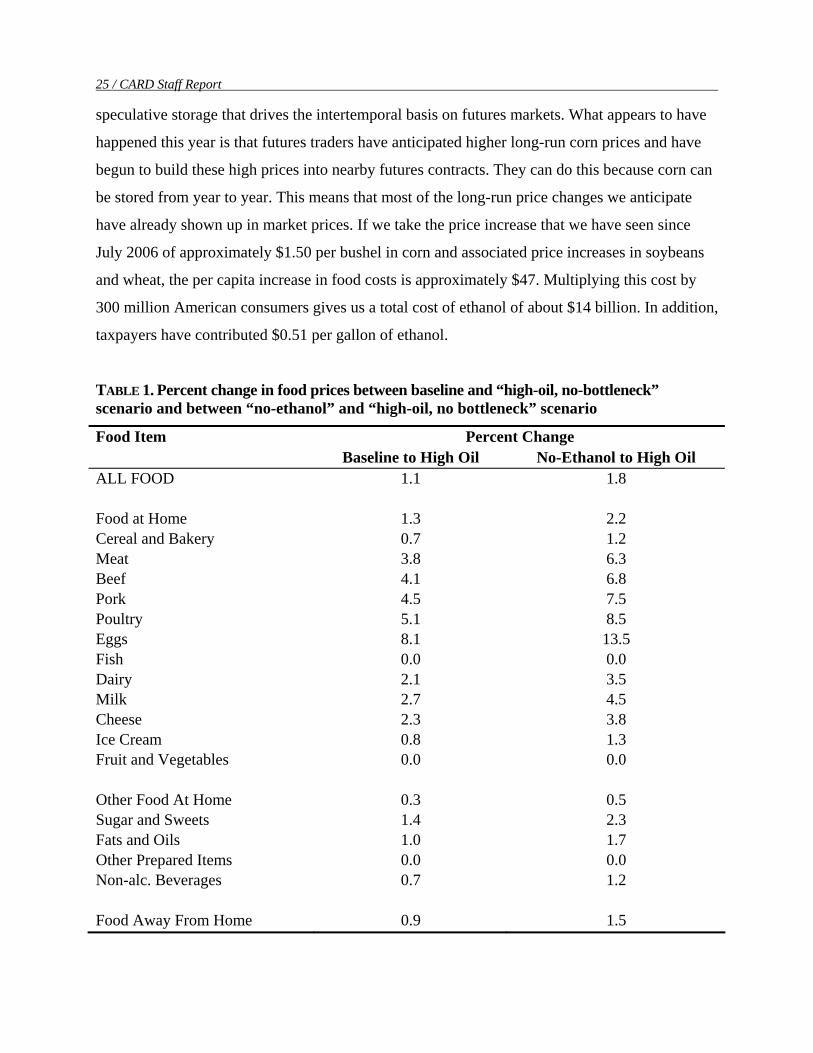
Table 1 shows the effect on food prices of the scenario for crude oil plus $10, no E-85
bottleneck, relative to the baseline and relative to an assumed “no-ethanol” corn price of $1.90.
From the baseline, egg prices increase by approximately 8% and poultry prices increase by
approximately 5%. Other meat and dairy prices increase by slightly smaller percentages. Overall
consumer expenditures on food would increase by about $40 per person from the baseline and by
about $67 from $1.90 corn.
Price Effects to Date The model calculates the market-clearing price in each year based on expected supply and
demand conditions in that year. The model does not contain equations that describe the kind of
25 / CARD Staff Report
speculative storage that drives the intertemporal basis on futures markets. What appears to have
happened this year is that futures traders have anticipated higher long-run corn prices and have
begun to build these high prices into nearby futures contracts. They can do this because corn can
be stored from year to year. This means that most of the long-run price changes we anticipate
have already shown up in market prices. If we take the price increase that we have seen since
July 2006 of approximately $1.50 per bushel in corn and associated price increases in soybeans
and wheat, the per capita increase in food costs is approximately $47. Multiplying this cost by
300 million American consumers gives us a total cost of ethanol of about $14 billion. In addition,
taxpayers have contributed $0.51 per gallon of ethanol.
TABLE 1. Percent change in food prices between baseline and “high-oil, no-bottleneck” scenario and between “no-ethanol” and “high-oil, no bottleneck” scenario
Food Item Percent Change Baseline to High Oil No-Ethanol to High Oil
ALL FOOD 1.1 1.8
Food at Home 1.3 2.2 Cereal and Bakery 0.7 1.2 Meat 3.8 6.3 Beef 4.1 6.8 Pork 4.5 7.5 Poultry 5.1 8.5 Eggs 8.1 13.5 Fish 0.0 0.0 Dairy 2.1 3.5 Milk 2.7 4.5 Cheese 2.3 3.8 Ice Cream 0.8 1.3 Fruit and Vegetables 0.0 0.0
Other Food At Home 0.3 0.5 Sugar and Sweets 1.4 2.3 Fats and Oils 1.0 1.7 Other Prepared Items 0.0 0.0 Non-alc. Beverages 0.7 1.2
Food Away From Home 0.9 1.5
Emerging Biofuels: Outlook of Effects / 26
Because world feed prices track U.S. feed prices, the rest of the world’s consumers would
also see higher food prices. To the extent that both feed and livestock markets are closely
integrated in all countries, the food price increases reported for the U.S. consumer would also be
felt by the rest of the world. However, consumers in the rest of the world tend to spend a lower
proportion of their food dollar on meat and dairy products relative to the U.S. consumer. Hence,
the percent increase in food prices would tend to be less. In addition, many countries do not have
free trade in either meat or feed grains, so trade barriers would need to be accounted for to obtain
a good estimate of the impact of U.S. ethanol on world food prices.
Three Caveats Note that we are modeling the direct effect of feed cost increases on food costs. That is, we
assume that livestock producers and retailers pass along only the additional feed cost and that
they do not add any other cost increases. Were we to assume that the livestock marketing chain
passed along price increases in percentage terms rather than in dollar terms, then the price effect
would be much larger. Moreover, we do not account for any food cost changes from other land-
intensive crops such as vegetables that are not in the model to increase. We have also ignored
second-round impacts such as those that might occur if employees request wage increases to
compensate for higher food costs. Because of all of these omissions, the food price impact results
should be considered a lower bound.
A second caveat concerns the acreage changes that would come about if the equilibrium
price of corn rises to $4.43 per bushel. We have assumed that yields for each U.S. producing
region remain fixed at their baseline levels despite significantly greater corn acreage. One would
think that increased corn plantings would begin to cause corn yields to decline because the
additional corn acreage would not be planted as much in rotation with soybeans and it would be
planted on increasingly marginal (lower-yielding) land outside of the Corn Belt. A decline in
corn yields would decrease the supply elasticity of corn production with respect to price so that
corn acreage would be smaller and other crop acreage would be greater than that reported. Total
ethanol production from corn would also be proportionately less than our results indicate. High
corn prices, however, are likely to counter this yield decline, as farmers would find it profitable
to manage their crops more intensely, and seed companies would find it profitable to invest
greater amounts in yield-increasing technologies. Whether the yield-decreasing effects of less
27 / CARD Staff Report
crop rotation and less-productive land are greater than the yield-increasing effects of high prices
cannot be known with certainty.
The last caveat has to do with ethanol trade policy. The no-bottleneck scenario assumes that
the U.S. ethanol tariff structure remains in place. If the tariffs were removed ($0.54 specific and
2.5% ad valorem), blenders would arbitrate between foreign and domestic sources of ethanol.
Margins of U.S. ethanol plants would be affected negatively and their expansion would be more
limited than reported, as they would receive the world ethanol price adjusted for transportation.
Crop price increases would be moderate and the impacts on food prices would be smaller than
those reported in Table 1. The world price of sugar would rise as sugar-cane ethanol production
would expand but with little consequence for the U.S. sugar price. The latter is not determined
by the world sugar market but rather by domestic market conditions and policy.
Impact of a Short Crop A major concern of livestock feeders is that they will not be able to compete with ethanol
producers in a short-crop year caused by, for example, a widespread drought in the Corn Belt.
With a large ethanol industry competing with livestock producers for corn, there is no doubt that
corn prices would increase significantly in a short-crop year. Economic theory and historical
events in 1995 suggest that corn prices would rise until operating margins of ethanol plants turn
negative, at which point plants would begin to shut down, thereby increasing the supply of corn
available to livestock feeders. The shut-down price can be inferred from Figures 5 and 6. If the
short-crop occurred in 2010, then prices would have to increase by about $0.65 per bushel to
induce ethanol plants to shut down.
However, what if ethanol plants were operating under a mandate? In this case, any required
adjustment in demand would occur outside the ethanol industry, which would continue to
operate, covering the increased cost of corn by passing on higher ethanol prices to blenders. To
see how the livestock industry would be affected by an ethanol mandate combined with a short
crop, U.S. regional yields of corn, soybeans, and wheat in 2012 were changed from their trend
levels by the same percentages that yields were observed to have changed from trend levels in
1988. The year 1988 was chosen because that was the most recent year of major drought in the
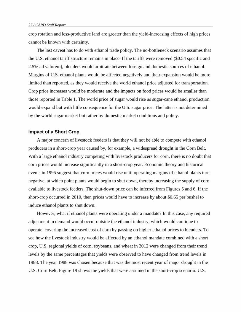
U.S. Corn Belt. Figure 19 shows the yields that were assumed in the short-crop scenario. U.S.
Emerging Biofuels: Outlook of Effects / 28
corn yields fall by about 25% in 2012. Soybean yields fall by about 18%, and wheat yields fall
by 11%.
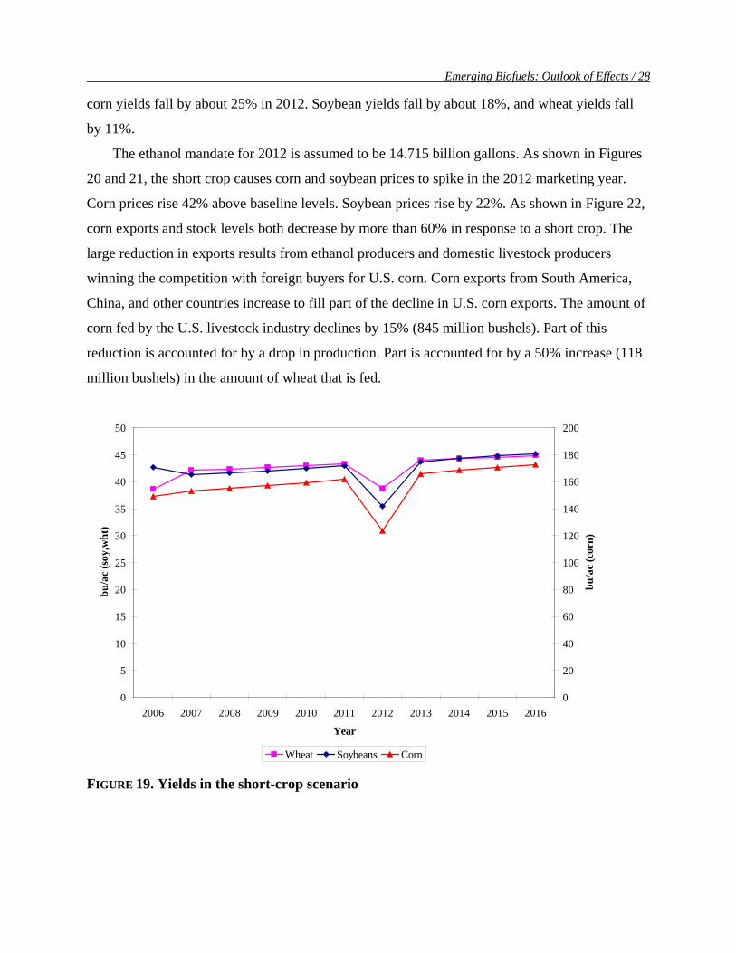
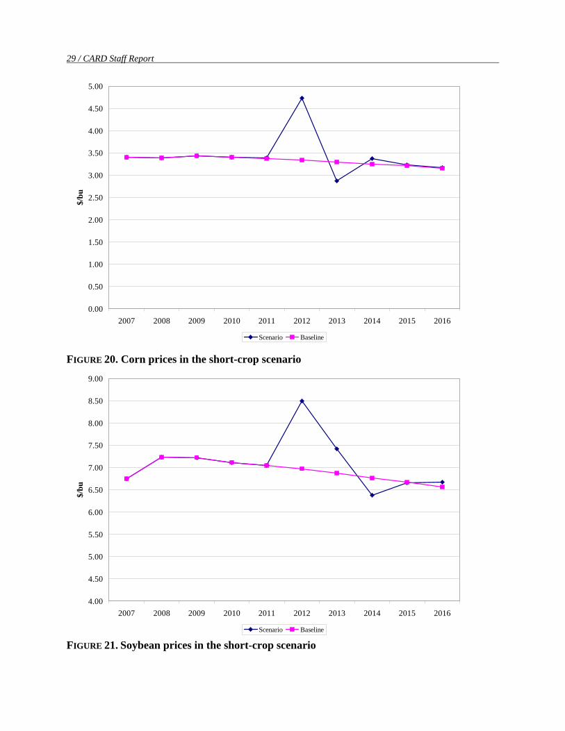
The ethanol mandate for 2012 is assumed to be 14.715 billion gallons. As shown in Figures
20 and 21, the short crop causes corn and soybean prices to spike in the 2012 marketing year.
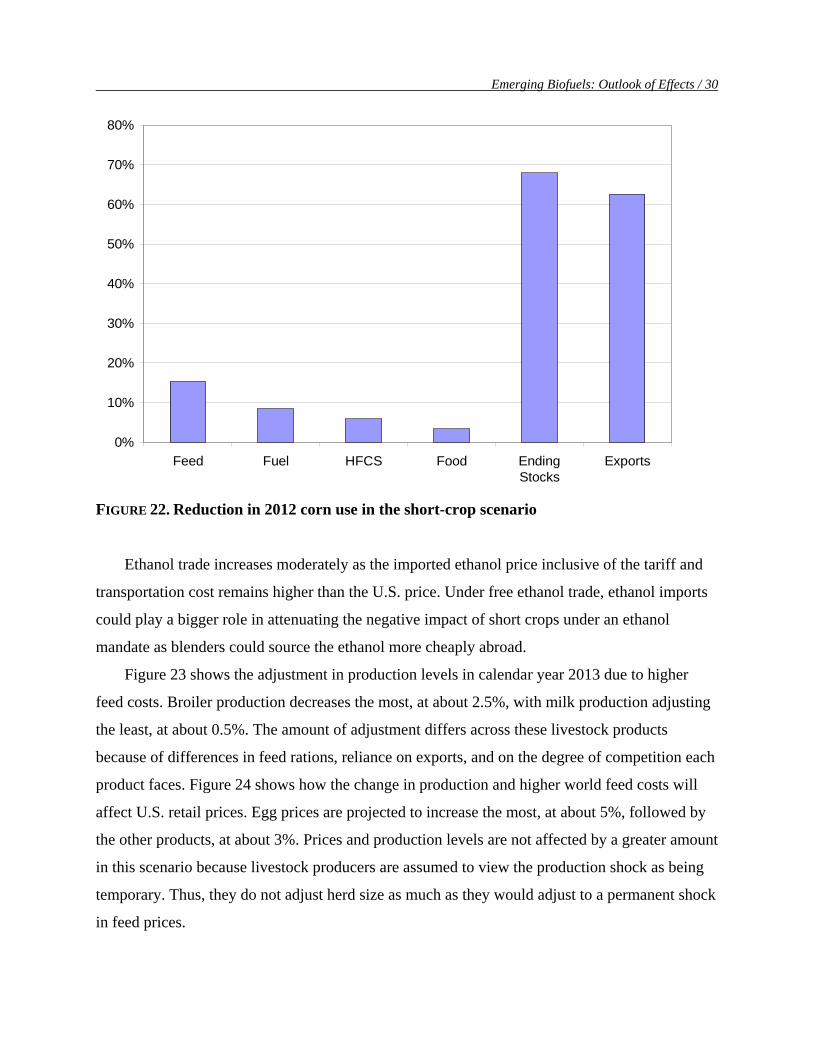
Corn prices rise 42% above baseline levels. Soybean prices rise by 22%. As shown in Figure 22,
corn exports and stock levels both decrease by more than 60% in response to a short crop. The
large reduction in exports results from ethanol producers and domestic livestock producers
winning the competition with foreign buyers for U.S. corn. Corn exports from South America,
China, and other countries increase to fill part of the decline in U.S. corn exports. The amount of
corn fed by the U.S. livestock industry declines by 15% (845 million bushels). Part of this
reduction is accounted for by a drop in production. Part is accounted for by a 50% increase (118
million bushels) in the amount of wheat that is fed.
0
5
10
15
20
25
30
35
40
45
50
2006 2007 2008 2009 2010 2011 2012 2013 2014 2015 2016
Year
bu/a
c (s
oy,w
ht)
0
20
40
60
80
100
120
140
160
180
200
bu/a
c (c
orn)
Wheat Soybeans Corn FIGURE 19. Yields in the short-crop scenario
29 / CARD Staff Report
0.00
0.50
1.00
1.50
2.00
2.50
3.00
3.50
4.00
4.50
5.00
2007 2008 2009 2010 2011 2012 2013 2014 2015 2016
$/bu
Scenario Baseline FIGURE 20. Corn prices in the short-crop scenario
4.00
4.50
5.00
5.50
6.00
6.50
7.00
7.50
8.00
8.50
9.00
2007 2008 2009 2010 2011 2012 2013 2014 2015 2016
$/bu
Scenario Baseline FIGURE 21. Soybean prices in the short-crop scenario
Emerging Biofuels: Outlook of Effects / 30
0%
10%
20%
30%
40%
50%
60%
70%
80%
Feed Fuel HFCS Food EndingStocks
Exports
FIGURE 22. Reduction in 2012 corn use in the short-crop scenario
Ethanol trade increases moderately as the imported ethanol price inclusive of the tariff and
transportation cost remains higher than the U.S. price. Under free ethanol trade, ethanol imports
could play a bigger role in attenuating the negative impact of short crops under an ethanol
mandate as blenders could source the ethanol more cheaply abroad.
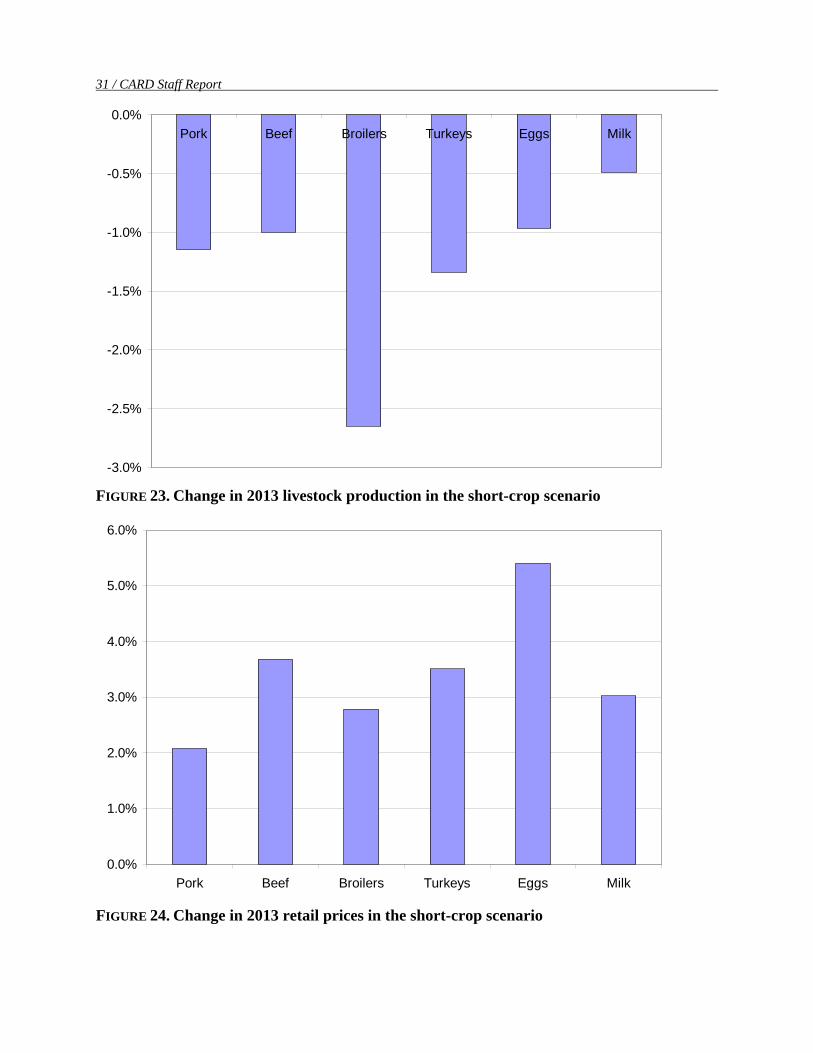
Figure 23 shows the adjustment in production levels in calendar year 2013 due to higher
feed costs. Broiler production decreases the most, at about 2.5%, with milk production adjusting
the least, at about 0.5%. The amount of adjustment differs across these livestock products
because of differences in feed rations, reliance on exports, and on the degree of competition each
product faces. Figure 24 shows how the change in production and higher world feed costs will
affect U.S. retail prices. Egg prices are projected to increase the most, at about 5%, followed by
the other products, at about 3%. Prices and production levels are not affected by a greater amount
in this scenario because livestock producers are assumed to view the production shock as being
temporary. Thus, they do not adjust herd size as much as they would adjust to a permanent shock
in feed prices.
31 / CARD Staff Report
-3.0%
-2.5%
-2.0%
-1.5%
-1.0%
-0.5%
0.0%Pork Beef Broilers Turkeys Eggs Milk
FIGURE 23. Change in 2013 livestock production in the short-crop scenario
0.0%
1.0%
2.0%
3.0%
4.0%
5.0%
6.0%
Pork Beef Broilers Turkeys Eggs Milk FIGURE 24. Change in 2013 retail prices in the short-crop scenario
Emerging Biofuels: Outlook of Effects / 32
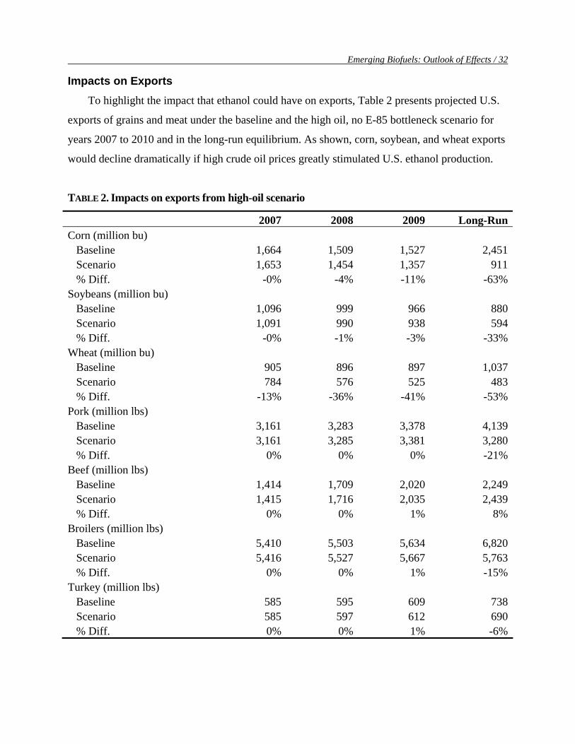
Impacts on Exports To highlight the impact that ethanol could have on exports, Table 2 presents projected U.S.
exports of grains and meat under the baseline and the high oil, no E-85 bottleneck scenario for
years 2007 to 2010 and in the long-run equilibrium. As shown, corn, soybean, and wheat exports
would decline dramatically if high crude oil prices greatly stimulated U.S. ethanol production.
TABLE 2. Impacts on exports from high-oil scenario
2007 2008 2009 Long-RunCorn (million bu) Baseline 1,664 1,509 1,527 2,451 Scenario 1,653 1,454 1,357 911 % Diff. -0% -4% -11% -63%Soybeans (million bu) Baseline 1,096 999 966 880 Scenario 1,091 990 938 594 % Diff. -0% -1% -3% -33%Wheat (million bu) Baseline 905 896 897 1,037 Scenario 784 576 525 483 % Diff. -13% -36% -41% -53%Pork (million lbs) Baseline 3,161 3,283 3,378 4,139 Scenario 3,161 3,285 3,381 3,280 % Diff. 0% 0% 0% -21%Beef (million lbs) Baseline 1,414 1,709 2,020 2,249 Scenario 1,415 1,716 2,035 2,439 % Diff. 0% 0% 1% 8%Broilers (million lbs) Baseline 5,410 5,503 5,634 6,820 Scenario 5,416 5,527 5,667 5,763 % Diff. 0% 0% 1% -15%Turkey (million lbs) Baseline 585 595 609 738 Scenario 585 597 612 690 % Diff. 0% 0% 1% -6%
33 / CARD Staff Report
In addition, exports of pork, broilers, and turkeys would decline, but by a smaller percentage
than crop exports would decline. The reason for this difference is that world demand for U.S.
meat is largely unaffected by higher feed-grain prices because the rest of the world’s livestock
producers also face higher feed prices. Total world meat consumption declines because of higher
prices, but U.S. producers still would find it profitable to supply world markets. Beef exports are
projected to increase because the price of beef relative to other meats declines.
State-Level Corn and Distillers Grains Projections To see how the expansion of the ethanol industry is changing the flow of corn and DG
across the United States, we now compare baseline and scenario state-level corn utilization rates.
State-level domestic surplus corn and DG is the amount or product remaining in a state after
accounting for ethanol, livestock feed, and other processing in a state. To do that for corn, we
estimated corn usage for ethanol and livestock feed by state and combined those estimates with
estimates of state corn processing for non-ethanol purposes and corn production numbers from
USDA. Based on the figures by state of corn used for ethanol, we computed the DG production
by state and estimated DG usage in livestock feed. Domestic surplus corn and DG are corn and
DG that are either maintained in stocks or available for export to other states or countries. We
estimated domestic surplus corn for 2004 and projections in 2010 for corn and DG under the two
scenarios.
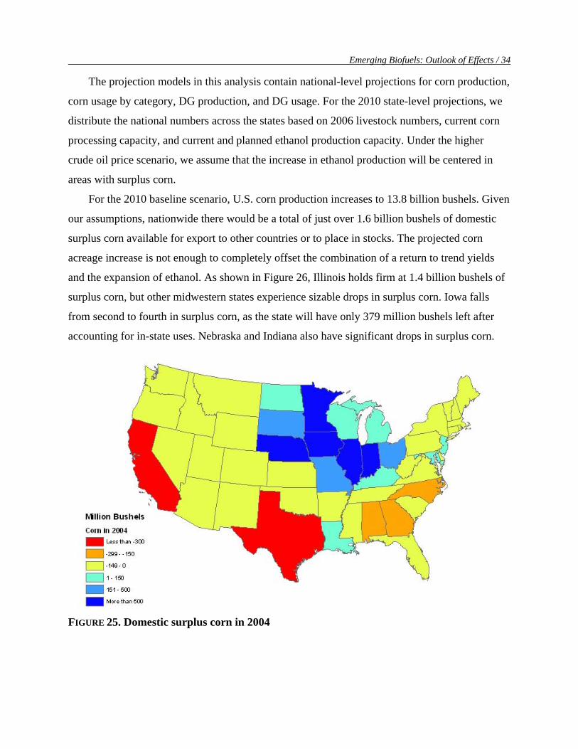
Figure 25 shows the state-level corn situation in 2004. The 2004 crop year was a record
breaker for corn, with U.S. corn production of 11.8 billion bushels. Domestic livestock
consumed over 6 billion bushels of that crop. Ethanol captured over 1 billion bushels, and other
corn processing took over 1 billion bushels as well. That left roughly 3 billion bushels of
domestic surplus corn for exports and stocks. As Figure 25 shows, the surplus corn came from
the upper Midwest. Sixteen states produced more corn than they used. Illinois had the most
surplus corn, at 1.4 billion bushels, but Iowa, Minnesota, Indiana, and Nebraska all had over 500
million bushels of surplus corn each. The major corn-importing states were California, Texas,
North Carolina, Georgia, and Alabama.
Emerging Biofuels: Outlook of Effects / 34
The projection models in this analysis contain national-level projections for corn production,
corn usage by category, DG production, and DG usage. For the 2010 state-level projections, we
distribute the national numbers across the states based on 2006 livestock numbers, current corn
processing capacity, and current and planned ethanol production capacity. Under the higher
crude oil price scenario, we assume that the increase in ethanol production will be centered in
areas with surplus corn.
For the 2010 baseline scenario, U.S. corn production increases to 13.8 billion bushels. Given
our assumptions, nationwide there would be a total of just over 1.6 billion bushels of domestic
surplus corn available for export to other countries or to place in stocks. The projected corn
acreage increase is not enough to completely offset the combination of a return to trend yields
and the expansion of ethanol. As shown in Figure 26, Illinois holds firm at 1.4 billion bushels of
surplus corn, but other midwestern states experience sizable drops in surplus corn. Iowa falls
from second to fourth in surplus corn, as the state will have only 379 million bushels left after
accounting for in-state uses. Nebraska and Indiana also have significant drops in surplus corn.
FIGURE 25. Domestic surplus corn in 2004
35 / CARD Staff Report
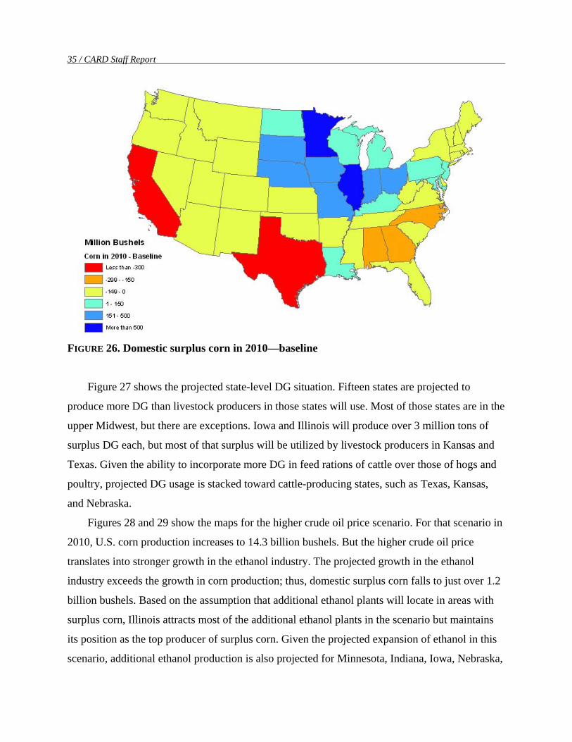
FIGURE 26. Domestic surplus corn in 2010—baseline
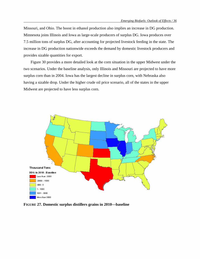
Figure 27 shows the projected state-level DG situation. Fifteen states are projected to
produce more DG than livestock producers in those states will use. Most of those states are in the
upper Midwest, but there are exceptions. Iowa and Illinois will produce over 3 million tons of
surplus DG each, but most of that surplus will be utilized by livestock producers in Kansas and
Texas. Given the ability to incorporate more DG in feed rations of cattle over those of hogs and
poultry, projected DG usage is stacked toward cattle-producing states, such as Texas, Kansas,
and Nebraska.
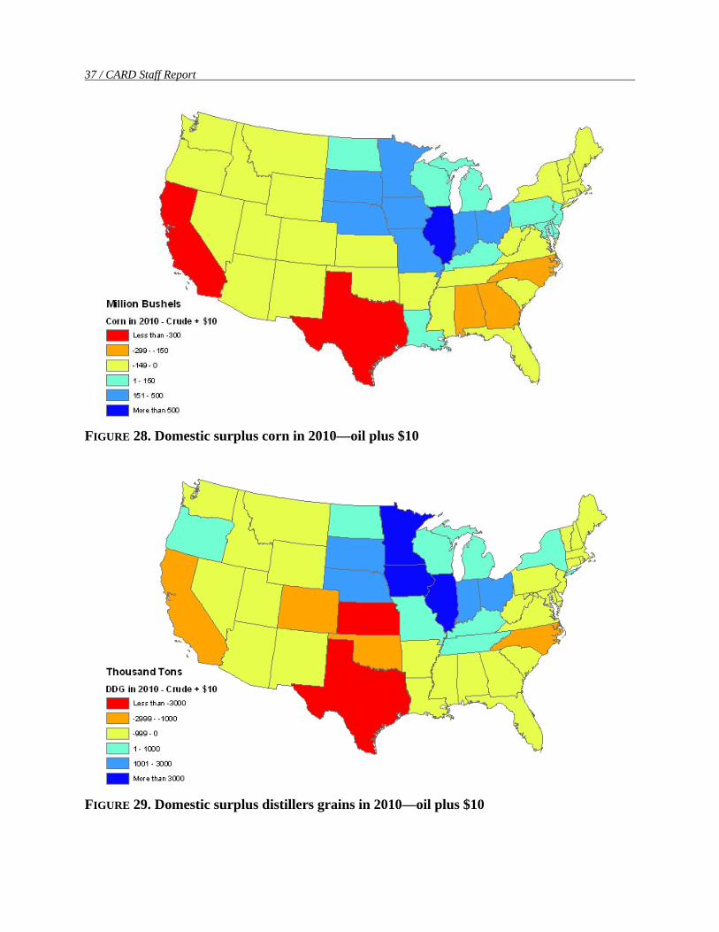
Figures 28 and 29 show the maps for the higher crude oil price scenario. For that scenario in
2010, U.S. corn production increases to 14.3 billion bushels. But the higher crude oil price
translates into stronger growth in the ethanol industry. The projected growth in the ethanol
industry exceeds the growth in corn production; thus, domestic surplus corn falls to just over 1.2
billion bushels. Based on the assumption that additional ethanol plants will locate in areas with
surplus corn, Illinois attracts most of the additional ethanol plants in the scenario but maintains
its position as the top producer of surplus corn. Given the projected expansion of ethanol in this
scenario, additional ethanol production is also projected for Minnesota, Indiana, Iowa, Nebraska,
Emerging Biofuels: Outlook of Effects / 36
Missouri, and Ohio. The boost in ethanol production also implies an increase in DG production.
Minnesota joins Illinois and Iowa as large-scale producers of surplus DG. Iowa produces over
7.5 million tons of surplus DG, after accounting for projected livestock feeding in the state. The
increase in DG production nationwide exceeds the demand by domestic livestock producers and
provides sizable quantities for export.
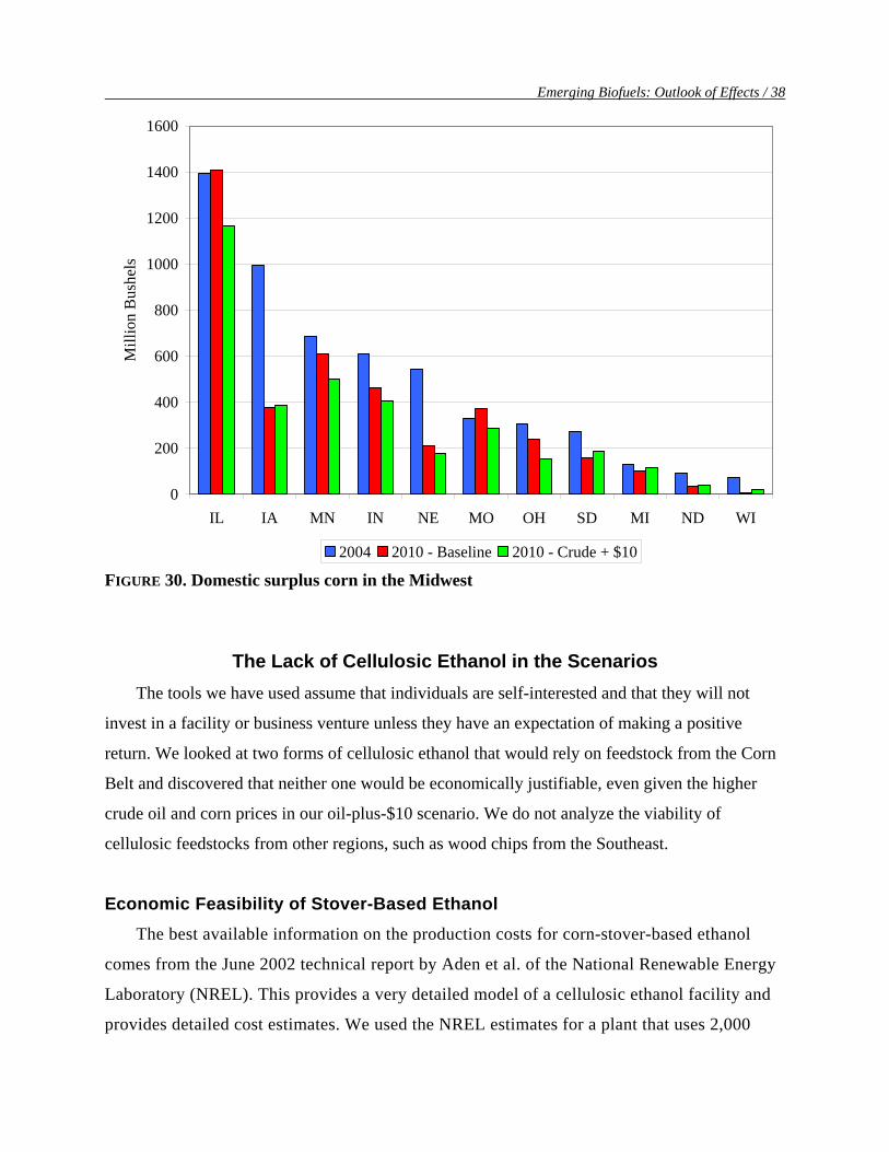
Figure 30 provides a more detailed look at the corn situation in the upper Midwest under the
two scenarios. Under the baseline analysis, only Illinois and Missouri are projected to have more
surplus corn than in 2004. Iowa has the largest decline in surplus corn, with Nebraska also
having a sizable drop. Under the higher crude oil price scenario, all of the states in the upper
Midwest are projected to have less surplus corn.
FIGURE 27. Domestic surplus distillers grains in 2010—baseline
37 / CARD Staff Report
FIGURE 28. Domestic surplus corn in 2010—oil plus $10
FIGURE 29. Domestic surplus distillers grains in 2010—oil plus $10
Emerging Biofuels: Outlook of Effects / 38
0
200
400
600
800
1000
1200
1400
1600
IL IA MN IN NE MO OH SD MI ND WI
Mill
ion
Bus
hels
2004 2010 - Baseline 2010 - Crude + $10
FIGURE 30. Domestic surplus corn in the Midwest
The Lack of Cellulosic Ethanol in the Scenarios The tools we have used assume that individuals are self-interested and that they will not
invest in a facility or business venture unless they have an expectation of making a positive
return. We looked at two forms of cellulosic ethanol that would rely on feedstock from the Corn
Belt and discovered that neither one would be economically justifiable, even given the higher
crude oil and corn prices in our oil-plus-$10 scenario. We do not analyze the viability of
cellulosic feedstocks from other regions, such as wood chips from the Southeast.
Economic Feasibility of Stover-Based Ethanol The best available information on the production costs for corn-stover-based ethanol
comes from the June 2002 technical report by Aden et al. of the National Renewable Energy
Laboratory (NREL). This provides a very detailed model of a cellulosic ethanol facility and
provides detailed cost estimates. We used the NREL estimates for a plant that uses 2,000
39 / CARD Staff Report
tons per day and produces 51 million gallons per year, as suggested by the report. This plant
has a 50-mile-radius draw area for stover. We assumed that the plant offers a plant-gate price
that attracts stover from the edge of this draw area.
While we agree with much of the research in this report, we disagree with one key
assumption. The report details all of the costs associated with the baling and transportation of
corn stover, and these calculations sum to $62 per dry metric ton. This is about $31 for a
1,265 pound bale of 15% moisture stover. The authors then arbitrarily assume that this cost
will be reduced to $33 per dry metric ton in the future through “improved collection.” We are
of the opinion that farmers and agricultural equipment manufacturers have already squeezed
costs from this system, and we do not expect these costs to fall dramatically. In fact, because
some of the costs are themselves transportation related, they would be higher under a higher
oil price scenario.
We compiled our own stover collection costs from Iowa State University Extension
(2006) for 1,265 pound bales as follows: baling, $10.10; staging, $2.25; and hauling, $15.00
($0.30 per mile for 50 miles). We excluded chopping charges of $8 per acre or $2 per bale
because we could not be sure in what form the plant would ideally like to receive these bales.
In addition, we used the NREL estimates of the required premium to farmers of $5.50/bale
and a lost fertilizer value of $4.00/bale. The total cost per delivered dry ton is $73.70. With
an assumed conversion of 70 gallons per ton, the raw material cost is $1.05 per gallon.
We then used the capital cost of $197.4 million from the NREL report amortized over 10
year at 10% interest with annual payments of $31.3 million to get a capital charge per gallon
of $0.61. We used the variable costs of 36¢ per gallon from Tables 30 and 32 of the NREL
report.
Table 3 compares these costs to those for a corn-based ethanol plant for a year in which
corn is worth $4.50 per bushel delivered to the plant. We assumed that the corn-based
ethanol plant could sell DG at $150 per ton and used the assumptions from the Elobeid et al.
report for the fixed and variable costs for this corn-based ethanol plant.
By its authors’ own admission, the NREL report is based on optimistic assumptions about
the process. In particular, the variable costs of running the plant are low because the NREL
report assumes dramatic reductions from current levels in the costs of the catalysts and enzymes,
and it assumes much lower labor costs than were used in the Elobeid et al. report. For example,
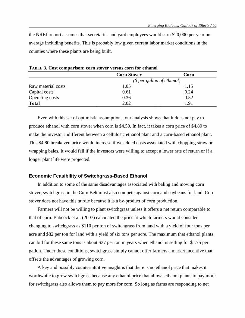
Emerging Biofuels: Outlook of Effects / 40
the NREL report assumes that secretaries and yard employees would earn $20,000 per year on
average including benefits. This is probably low given current labor market conditions in the
counties where these plants are being built.
TABLE 3. Cost comparison: corn stover versus corn for ethanol Corn Stover Corn ($ per gallon of ethanol) Raw material costs 1.05 1.15 Capital costs 0.61 0.24 Operating costs 0.36 0.52 Total 2.02 1.91
Even with this set of optimistic assumptions, our analysis shows that it does not pay to
produce ethanol with corn stover when corn is $4.50. In fact, it takes a corn price of $4.80 to
make the investor indifferent between a cellulosic ethanol plant and a corn-based ethanol plant.
This $4.80 breakeven price would increase if we added costs associated with chopping straw or
wrapping bales. It would fall if the investors were willing to accept a lower rate of return or if a
longer plant life were projected.
Economic Feasibility of Switchgrass-Based Ethanol In addition to some of the same disadvantages associated with baling and moving corn
stover, switchgrass in the Corn Belt must also compete against corn and soybeans for land. Corn
stover does not have this hurdle because it is a by-product of corn production.
Farmers will not be willing to plant switchgrass unless it offers a net return comparable to
that of corn. Babcock et al. (2007) calculated the price at which farmers would consider
changing to switchgrass as $110 per ton of switchgrass from land with a yield of four tons per
acre and $82 per ton for land with a yield of six tons per acre. The maximum that ethanol plants
can bid for these same tons is about $37 per ton in years when ethanol is selling for $1.75 per
gallon. Under these conditions, switchgrass simply cannot offer farmers a market incentive that
offsets the advantages of growing corn.
A key and possibly counterintuitive insight is that there is no ethanol price that makes it
worthwhile to grow switchgrass because any ethanol price that allows ethanol plants to pay more
for switchgrass also allows them to pay more for corn. So long as farms are responding to net
41 / CARD Staff Report
returns in a rational manner and so long as ethanol plants are paying their breakeven price for
raw material, farmers will plant corn as an energy crop. Switchgrass in the Corn Belt will make
economic sense only if it receives an additional subsidy that is not provided for corn-based
ethanol.
Biodiesel The same logic that works against switchgrass also works against biodiesel. The main crop
for U.S. production of biodiesel is soybeans. Soybeans produce fewer bushels per acre and less
energy value per bushel than corn, so as long as markets are working, and in equilibrium,
producers targeting energy crops would choose corn over soybeans.
References
Aden, A., M. Ruth, K. Ibsen, J. Jechura, K. Neeves, J. Sheehan, B. Wallace, L. Montague, A. Slayton, and J. Lukas. 2002. “Lignocellulosic Biomass to Ethanol Process Design and Economics Utilizing Co-Current Dilute Acid Prehydrolysis and Enzymatic Hydrolysis for Corn Stover.” Technical Report NREL/TP-510-32438, June, National Renewable Energy Laboratory, Golden, CO.
Babcock, B.A., P.W. Gassman, M.J. Jha, and C.L. Kling. 2007. “Adoption Subsidies and Environmental Impacts of Alternative Energy Crops.” CARD Briefing Paper 07-BP 50, Center for Agricultural and Rural Development, Iowa State University.
Elobeid, A., S. Tokgoz, D.J. Hayes, B.A. Babcock, and C.E. Hart. 2006. “The Long-Run Impact of Corn-Based Ethanol on the Grain, Oilseed, and Livestock Sectors: A Preliminary Assessment.” Briefing Paper 06-BP 49, Center for Agricultural and Rural Development, Iowa State University.
Iowa State University Extension. 2006. “2006 Iowa Farm Custom Rate Survey.”Ag Decision Maker, File A3-10, FM 1698. Prepared by W. Edwards and D. Smith. Revised March 2006.
Shurson, G.C. 2004. “Overview of Production and Nutrient Content of DDGS—Poultry, Swine, and Ruminants.” Presented at U.S. Grains Council Shortcourse for Canadian Animal Nutritionists, St. Paul, MN, October 28.

Appendix A
Long-Run Equilibrium Results for U.S. Crops and Livestock
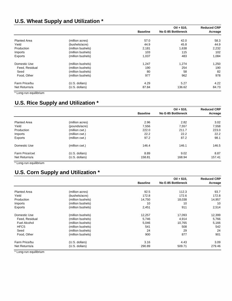
U.S. Wheat Supply and Utilization *
BaselineOil + $10,
No E-85 BottleneckReduced CRP
Acreage
Planted Area (million acres) 57.0 42.0 58.3Yield (bushels/acre) 44.9 45.8 44.9Production (million bushels) 2,181 1,638 2,232Imports (million bushels) 103 115 102Exports (million bushels) 1,037 483 1,084
Domestic Use (million bushels) 1,247 1,274 1,250 Feed, Residual (million bushels) 190 254 190 Seed (million bushels) 80 58 82 Food, Other (million bushels) 977 962 978
Farm Price/bu (U.S. dollars) 4.29 5.27 4.22Net Returns/a (U.S. dollars) 87.84 136.62 84.73
* Long-run equilibrium
U.S. Rice Supply and Utilization *
BaselineOil + $10,
No E-85 BottleneckReduced CRP
Acreage
Planted Area (million acres) 2.96 2.82 3.02Yield (pounds/acre) 7,556 7,557 7,558Production (million cwt.) 222.0 211.7 223.0Imports (million cwt.) 22.2 22.2 22.2Exports (million cwt.) 97.2 87.2 98.1
Domestic Use (million cwt.) 146.4 146.1 146.5
Farm Price/cwt (U.S. dollars) 8.89 9.02 8.87Net Returns/a (U.S. dollars) 158.81 168.94 157.41
* Long-run equilibrium
U.S. Corn Supply and Utilization *
BaselineOil + $10,
No E-85 BottleneckReduced CRP
Acreage
Planted Area (million acres) 92.5 112.3 93.7Yield (bushels/acre) 172.8 172.6 172.8Production (million bushels) 14,750 18,038 14,957Imports (million bushels) 10 10 10Exports (million bushels) 2,451 911 2,514
Domestic Use (million bushels) 12,257 17,093 12,399 Feed, Residual (million bushels) 5,746 4,914 5,766 Fuel Alcohol (million bushels) 5,046 10,765 5,166 HFCS (million bushels) 541 508 542 Seed (million bushels) 24 29 24 Food, Other (million bushels) 900 877 901
Farm Price/bu (U.S. dollars) 3.16 4.43 3.09Net Returns/a (U.S. dollars) 290.89 509.71 279.46
* Long-run equilibrium
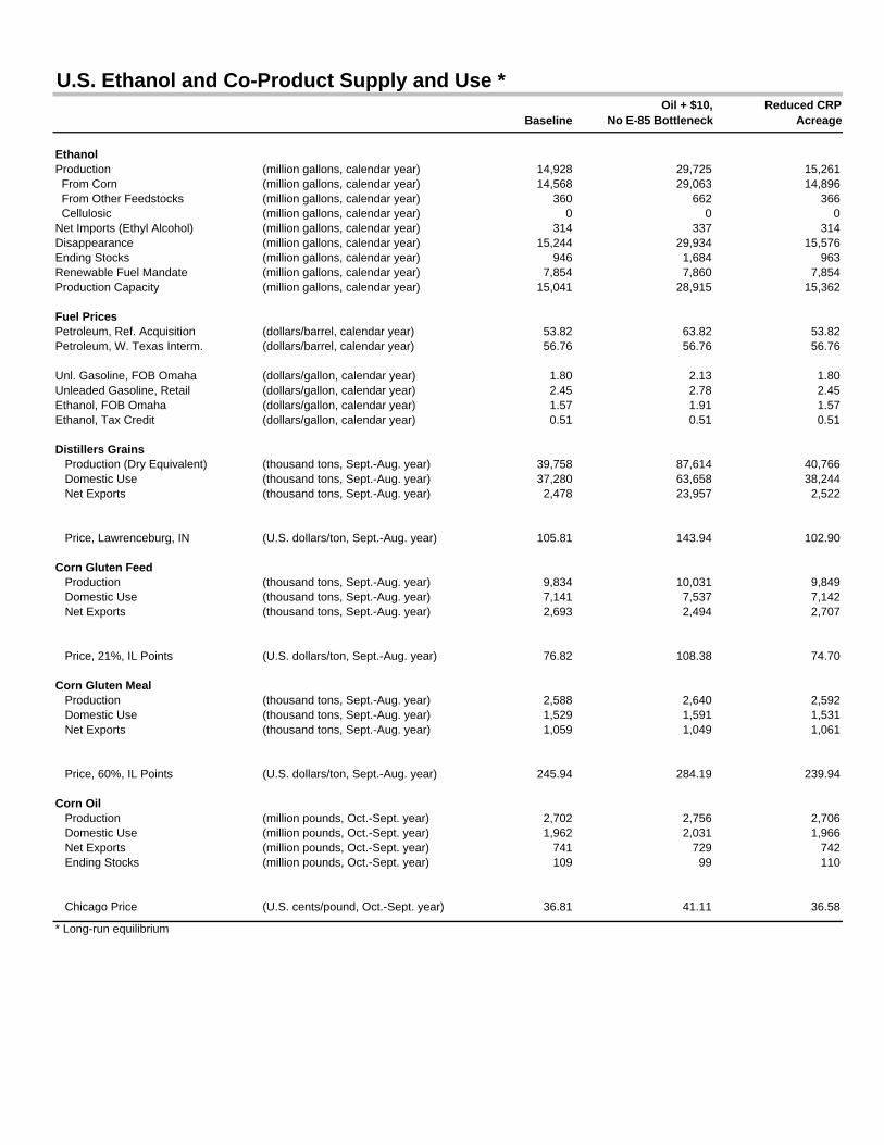
U.S. Ethanol and Co-Product Supply and Use *
BaselineOil + $10,
No E-85 BottleneckReduced CRP
Acreage
EthanolProduction (million gallons, calendar year) 14,928 29,725 15,261 From Corn (million gallons, calendar year) 14,568 29,063 14,896 From Other Feedstocks (million gallons, calendar year) 360 662 366 Cellulosic (million gallons, calendar year) 0 0 0Net Imports (Ethyl Alcohol) (million gallons, calendar year) 314 337 314Disappearance (million gallons, calendar year) 15,244 29,934 15,576Ending Stocks (million gallons, calendar year) 946 1,684 963Renewable Fuel Mandate (million gallons, calendar year) 7,854 7,860 7,854Production Capacity (million gallons, calendar year) 15,041 28,915 15,362
Fuel PricesPetroleum, Ref. Acquisition (dollars/barrel, calendar year) 53.82 63.82 53.82Petroleum, W. Texas Interm. (dollars/barrel, calendar year) 56.76 56.76 56.76
Unl. Gasoline, FOB Omaha (dollars/gallon, calendar year) 1.80 2.13 1.80Unleaded Gasoline, Retail (dollars/gallon, calendar year) 2.45 2.78 2.45Ethanol, FOB Omaha (dollars/gallon, calendar year) 1.57 1.91 1.57Ethanol, Tax Credit (dollars/gallon, calendar year) 0.51 0.51 0.51
Distillers Grains Production (Dry Equivalent) (thousand tons, Sept.-Aug. year) 39,758 87,614 40,766 Domestic Use (thousand tons, Sept.-Aug. year) 37,280 63,658 38,244 Net Exports (thousand tons, Sept.-Aug. year) 2,478 23,957 2,522
Price, Lawrenceburg, IN (U.S. dollars/ton, Sept.-Aug. year) 105.81 143.94 102.90
Corn Gluten Feed Production (thousand tons, Sept.-Aug. year) 9,834 10,031 9,849 Domestic Use (thousand tons, Sept.-Aug. year) 7,141 7,537 7,142 Net Exports (thousand tons, Sept.-Aug. year) 2,693 2,494 2,707
Price, 21%, IL Points (U.S. dollars/ton, Sept.-Aug. year) 76.82 108.38 74.70
Corn Gluten Meal Production (thousand tons, Sept.-Aug. year) 2,588 2,640 2,592 Domestic Use (thousand tons, Sept.-Aug. year) 1,529 1,591 1,531 Net Exports (thousand tons, Sept.-Aug. year) 1,059 1,049 1,061
Price, 60%, IL Points (U.S. dollars/ton, Sept.-Aug. year) 245.94 284.19 239.94
Corn Oil Production (million pounds, Oct.-Sept. year) 2,702 2,756 2,706 Domestic Use (million pounds, Oct.-Sept. year) 1,962 2,031 1,966 Net Exports (million pounds, Oct.-Sept. year) 741 729 742 Ending Stocks (million pounds, Oct.-Sept. year) 109 99 110
Chicago Price (U.S. cents/pound, Oct.-Sept. year) 36.81 41.11 36.58
* Long-run equilibrium
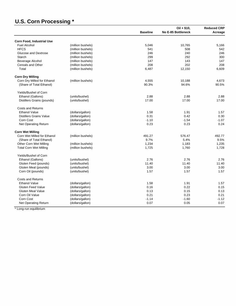
U.S. Corn Processing *
BaselineOil + $10,
No E-85 BottleneckReduced CRP
Acreage
Corn Food, Industrial Use Fuel Alcohol (million bushels) 5,046 10,765 5,166 HFCS (million bushels) 541 508 542 Glucose and Dextrose (million bushels) 246 240 246 Starch (million bushels) 299 292 300 Beverage Alcohol (million bushels) 147 143 147 Cereals and Other (million bushels) 208 202 208 Total (million bushels) 6,487 12,150 6,609
Corn Dry Milling Corn Dry Milled for Ethanol (million bushels) 4,555 10,188 4,673 (Share of Total Ethanol) 90.3% 94.6% 90.5%
Yields/Bushel of Corn Ethanol (Gallons) (units/bushel) 2.88 2.88 2.88 Distillers Grains (pounds) (units/bushel) 17.00 17.00 17.00
Costs and Returns Ethanol Value (dollars/gallon) 1.58 1.91 1.57 Distillers Grains Value (dollars/gallon) 0.31 0.42 0.30 Corn Cost (dollars/gallon) -1.10 -1.54 -1.07 Net Operating Return (dollars/gallon) 0.23 0.23 0.24
Corn Wet Milling Corn Wet Milled for Ethanol (million bushels) 491.27 576.47 492.77 (Share of Total Ethanol) 9.7% 5.4% 9.5% Other Corn Wet Milling (million bushels) 1,234 1,183 1,235 Total Corn Wet Milling (million bushels) 1,725 1,760 1,728
Yields/Bushel of Corn Ethanol (Gallons) (units/bushel) 2.76 2.76 2.76 Gluten Feed (pounds) (units/bushel) 11.40 11.40 11.40 Gluten Meal (pounds) (units/bushel) 3.00 3.00 3.00 Corn Oil (pounds) (units/bushel) 1.57 1.57 1.57
Costs and Returns Ethanol Value (dollars/gallon) 1.58 1.91 1.57 Gluten Feed Value (dollars/gallon) 0.16 0.22 0.15 Gluten Meal Value (dollars/gallon) 0.13 0.15 0.13 Corn Oil Value (dollars/gallon) 0.21 0.23 0.21 Corn Cost (dollars/gallon) -1.14 -1.60 -1.12 Net Operating Return (dollars/gallon) 0.07 0.05 0.07
* Long-run equilibrium
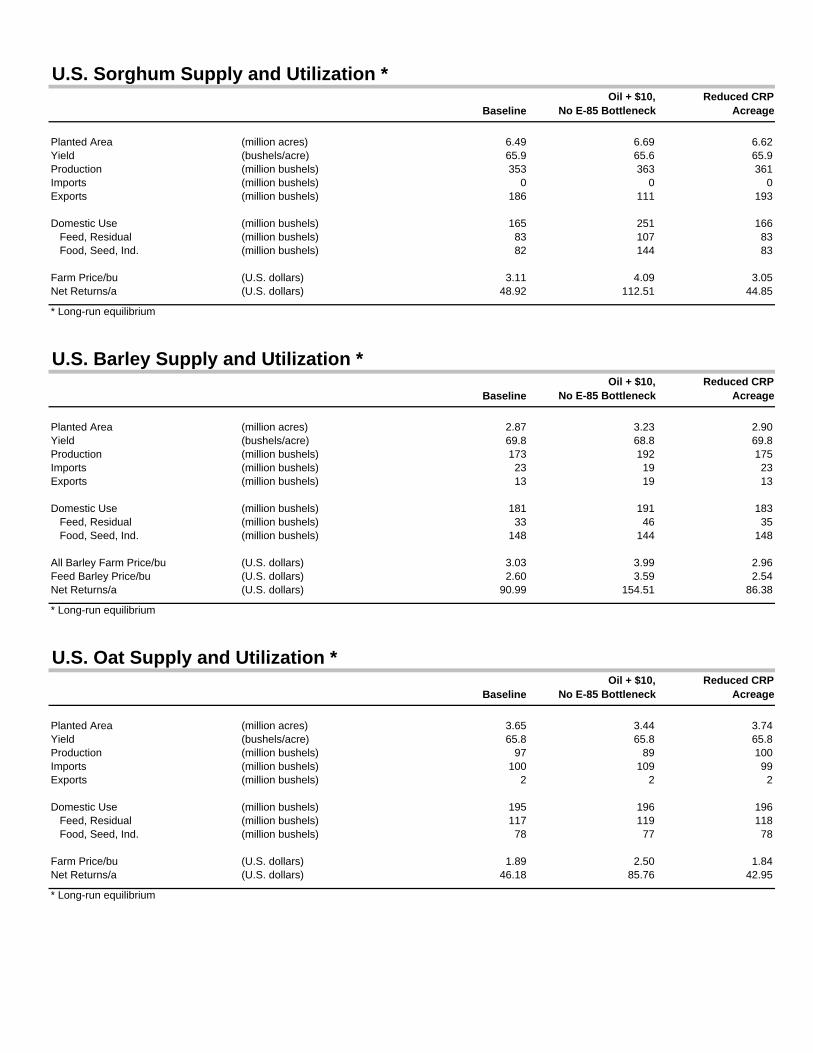
U.S. Sorghum Supply and Utilization *
BaselineOil + $10,
No E-85 BottleneckReduced CRP
Acreage
Planted Area (million acres) 6.49 6.69 6.62Yield (bushels/acre) 65.9 65.6 65.9Production (million bushels) 353 363 361Imports (million bushels) 0 0 0Exports (million bushels) 186 111 193
Domestic Use (million bushels) 165 251 166 Feed, Residual (million bushels) 83 107 83 Food, Seed, Ind. (million bushels) 82 144 83
Farm Price/bu (U.S. dollars) 3.11 4.09 3.05Net Returns/a (U.S. dollars) 48.92 112.51 44.85
* Long-run equilibrium
U.S. Barley Supply and Utilization *
BaselineOil + $10,
No E-85 BottleneckReduced CRP
Acreage
Planted Area (million acres) 2.87 3.23 2.90Yield (bushels/acre) 69.8 68.8 69.8Production (million bushels) 173 192 175Imports (million bushels) 23 19 23Exports (million bushels) 13 19 13
Domestic Use (million bushels) 181 191 183 Feed, Residual (million bushels) 33 46 35 Food, Seed, Ind. (million bushels) 148 144 148
All Barley Farm Price/bu (U.S. dollars) 3.03 3.99 2.96Feed Barley Price/bu (U.S. dollars) 2.60 3.59 2.54Net Returns/a (U.S. dollars) 90.99 154.51 86.38
* Long-run equilibrium
U.S. Oat Supply and Utilization *
BaselineOil + $10,
No E-85 BottleneckReduced CRP
Acreage
Planted Area (million acres) 3.65 3.44 3.74Yield (bushels/acre) 65.8 65.8 65.8Production (million bushels) 97 89 100Imports (million bushels) 100 109 99Exports (million bushels) 2 2 2
Domestic Use (million bushels) 195 196 196 Feed, Residual (million bushels) 117 119 118 Food, Seed, Ind. (million bushels) 78 77 78
Farm Price/bu (U.S. dollars) 1.89 2.50 1.84Net Returns/a (U.S. dollars) 46.18 85.76 42.95
* Long-run equilibrium
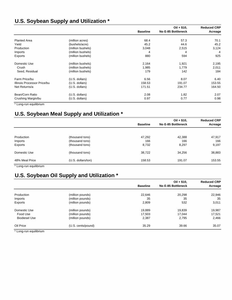
U.S. Soybean Supply and Utilization *
BaselineOil + $10,
No E-85 BottleneckReduced CRP
Acreage
Planted Area (million acres) 68.4 57.3 70.1Yield (bushels/acre) 45.2 44.6 45.2Production (million bushels) 3,048 2,515 3,124Imports (million bushels) 4 4 4Exports (million bushels) 880 594 925
Domestic Use (million bushels) 2,164 1,921 2,195 Crush (million bushels) 1,985 1,779 2,011 Seed, Residual (million bushels) 179 142 184
Farm Price/bu (U.S. dollars) 6.56 8.07 6.40Illinois Processor Price/bu (U.S. dollars) 158.53 191.07 153.55Net Returns/a (U.S. dollars) 171.51 234.77 164.50
Bean/Corn Ratio (U.S. dollars) 2.08 1.82 2.07Crushing Margin/bu (U.S. dollars) 0.97 0.77 0.98
* Long-run equilibrium
U.S. Soybean Meal Supply and Utilization *
BaselineOil + $10,
No E-85 BottleneckReduced CRP
Acreage
Production (thousand tons) 47,292 42,388 47,917Imports (thousand tons) 166 166 166Exports (thousand tons) 8,732 8,297 9,197
Domestic Use (thousand tons) 38,722 34,256 38,883
48% Meal Price (U.S. dollars/ton) 158.53 191.07 153.55
* Long-run equilibrium
U.S. Soybean Oil Supply and Utilization *
BaselineOil + $10,
No E-85 BottleneckReduced CRP
Acreage
Production (million pounds) 22,646 20,298 22,946Imports (million pounds) 35 35 35Exports (million pounds) 2,809 532 3,011
Domestic Use (million pounds) 19,889 19,839 19,987 Food Use (million pounds) 17,503 17,044 17,521 Biodiesel Use (million pounds) 2,387 2,795 2,466
Oil Price (U.S. cents/pound) 35.29 39.66 35.07
* Long-run equilibrium
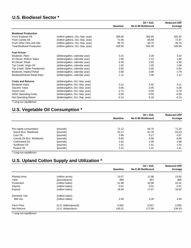
U.S. Biodiesel Sector *
BaselineOil + $10,
No E-85 BottleneckReduced CRP
Acreage
Biodiesel ProductionFrom Soybean Oil (million gallons, Oct.-Sep. year) 309.95 362.95 320.32From Canola Oil (million gallons, Oct.-Sep. year) 71.90 94.69 72.97From Other Fats and Oils (million gallons, Oct.-Sep. year) 46.70 46.70 46.70Total Biodiesel Production (million gallons, Oct.-Sep. year) 428.55 504.35 439.99
Fuel Prices*Biodiesel, Plant (dollars/gallon, calendar year) 3.10 3.39 3.10#2 Diesel, Refiner Sales (dollars/gallon, calendar year) 1.80 2.13 1.80#2 Diesel, Retail (dollars/gallon, calendar year) 2.49 2.82 2.49Tax Credit, Virgin Oil (dollars/gallon, calendar year) 1.00 1.00 1.00Tax Credit, Other Feedstocks (dollars/gallon, calendar year) 0.50 0.50 0.50Biodiesel, Implied Retail (dollars/gallon, calendar year) 2.80 3.08 2.79Biodiesel/Diesel Retail Ratio (dollars/gallon, calendar year) 1.12 1.09 1.12
Costs and Returns (dollars/gallon, Oct.-Sep. year)Biodiesel Value (dollars/gallon, Oct.-Sep. year) 3.12 3.42 3.11Glycerin Value (dollars/gallon, Oct.-Sep. year) 0.05 0.05 0.05Soyoil Cost (dollars/gallon, Oct.-Sep. year) -2.72 -3.05 -2.70Other Operating Costs (dollars/gallon, Oct.-Sep. year) -0.59 -0.59 -0.59Net Operating Return (dollars/gallon, Oct.-Sep. year) -0.14 -0.18 -0.13
* Long-run equilibrium
U.S. Vegetable Oil Consumption *
BaselineOil + $10,
No E-85 BottleneckReduced CRP
Acreage
Per-capita consumption (pounds) 71.12 69.70 71.24 Soyoil (Exc. Biodiesel) (pounds) 53.17 51.78 53.23 Corn Oil (pounds) 5.96 6.17 5.97 Canola Oil (Exc. Biodiesel) (pounds) 6.65 6.56 6.65 Cottonseed Oil (pounds) 2.62 2.48 2.68 Sunflower Oil (pounds) 1.51 1.51 1.51 Peanut Oil (pounds) 1.21 1.21 1.21
* Long-run equilibrium
U.S. Upland Cotton Supply and Utilization *
BaselineOil + $10,
No E-85 BottleneckReduced CRP
Acreage
Planted Area (million acres) 13.57 12.98 13.83Yield (pounds/acre) 859 857 859Production (million bales) 21.98 20.96 22.41Imports (million bales) 0.01 0.01 0.01Exports (million bales) 18.56 17.67 18.92
Domestic Use (million bales) Mill Use (million bales) 3.39 3.26 3.46
Farm Price (U.S. dollars/pound) 0.602 0.621 0.595Net Returns (U.S. dollars/acre) 145.51 177.99 136.33
* Long-run equilibrium
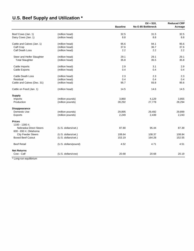
U.S. Beef Supply and Utilization *
BaselineOil + $10,
No E-85 BottleneckReduced CRP
Acreage
Beef Cows (Jan. 1) (million head) 32.5 31.5 32.5Dairy Cows (Jan. 1) (million head) 8.8 8.8 8.8
Cattle and Calves (Jan. 1) (million head) 95.6 94.1 95.6 Calf Crop (million head) 37.6 36.7 37.6 Calf Death Loss (million head) 2.2 2.2 2.2
Steer and Heifer Slaughter (million head) 29.1 29.1 29.1 Total Slaughter (million head) 35.8 35.5 35.8
Cattle Imports (million head) 2.9 3.1 2.9 Cattle Exports (million head) 0.4 0.4 0.4
Cattle Death Loss (million head) 2.3 2.3 2.3 Residual (million head) 0.4 0.4 0.4Cattle and Calves (Dec. 31) (million head) 95.7 93.8 95.6
Cattle on Feed (Jan. 1) (million head) 14.5 14.6 14.5
Supply Imports (million pounds) 3,860 4,129 3,855 Production (million pounds) 28,292 27,778 28,294
Disappearance Domestic Use (million pounds) 29,895 29,492 29,899 Exports (million pounds) 2,249 2,439 2,243
Prices 1100 - 1300 #, Nebraska Direct Steers (U.S. dollars/cwt.) 87.80 95.44 87.39 600 - 650 #, Oklahoma City Feeder Steers (U.S. dollars/cwt.) 108.64 108.37 108.84 Boxed Beef Cutout (U.S. dollars/cwt.) 153.19 164.28 152.55
Beef Retail (U.S. dollars/pound) 4.52 4.71 4.51
Net Returns Cow - Calf (U.S. dollars/cow) 20.68 20.68 20.19
* Long-run equilibrium
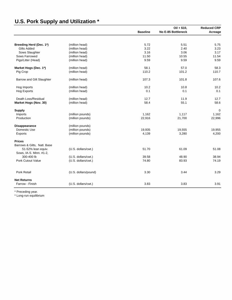
U.S. Pork Supply and Utilization *
BaselineOil + $10,
No E-85 BottleneckReduced CRP
Acreage
Breeding Herd (Dec. 1*) (million head) 5.72 5.51 5.75 Gilts Added (million head) 3.22 2.40 3.23 Sows Slaughter (million head) 3.16 3.06 3.17 Sows Farrowed (million head) 11.50 10.55 11.54 Pigs/Litter (Head) (million head) 9.59 9.59 9.59
Market Hogs (Dec. 1*) (million head) 58.1 57.0 58.3 Pig Crop (million head) 110.2 101.2 110.7
Barrow and Gilt Slaughter (million head) 107.3 101.8 107.6
Hog Imports (million head) 10.2 10.8 10.2 Hog Exports (million head) 0.1 0.1 0.1
Death Loss/Residual (million head) 12.7 11.9 12.7Market Hogs (Nov. 30) (million head) 58.4 55.1 58.6
Supply 0 Imports (million pounds) 1,162 1,117 1,162 Production (million pounds) 22,916 21,700 22,996
Disappearance (million pounds) Domestic Use (million pounds) 19,935 19,555 19,955 Exports (million pounds) 4,139 3,280 4,200
PricesBarrows & Gilts, Natl. Base 51-52% lean equiv. (U.S. dollars/cwt.) 51.70 61.09 51.08 Sows, IA-S. Minn. #1-2, 300-400 lb (U.S. dollars/cwt.) 39.58 48.90 38.94 Pork Cutout Value (U.S. dollars/cwt.) 74.80 83.93 74.19
Pork Retail (U.S. dollars/pound) 3.30 3.44 3.29
Net Returns Farrow - Finish (U.S. dollars/cwt.) 3.83 3.83 3.91
* Preceding year.* Long-run equilibrium
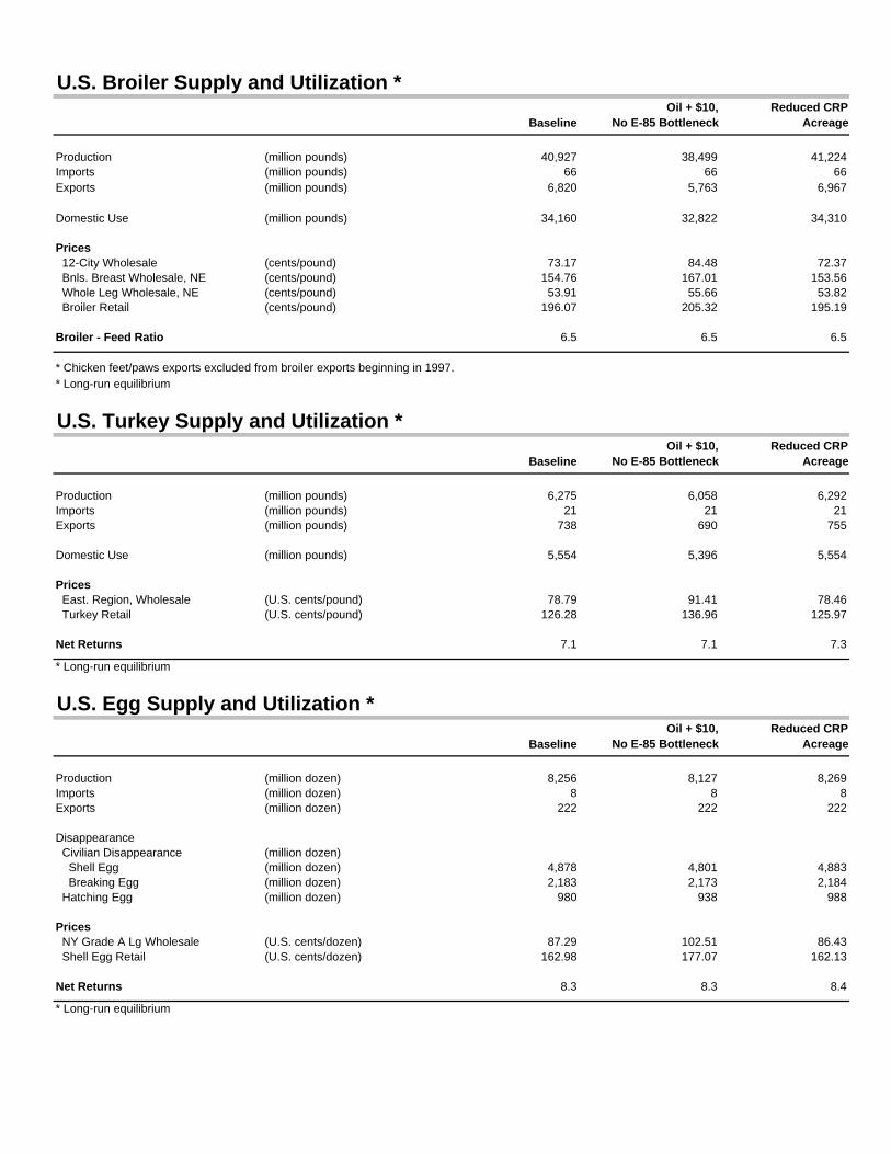
U.S. Broiler Supply and Utilization *
BaselineOil + $10,
No E-85 BottleneckReduced CRP
Acreage
Production (million pounds) 40,927 38,499 41,224Imports (million pounds) 66 66 66Exports (million pounds) 6,820 5,763 6,967
Domestic Use (million pounds) 34,160 32,822 34,310
Prices 12-City Wholesale (cents/pound) 73.17 84.48 72.37 Bnls. Breast Wholesale, NE (cents/pound) 154.76 167.01 153.56 Whole Leg Wholesale, NE (cents/pound) 53.91 55.66 53.82 Broiler Retail (cents/pound) 196.07 205.32 195.19
Broiler - Feed Ratio 6.5 6.5 6.5
* Chicken feet/paws exports excluded from broiler exports beginning in 1997.* Long-run equilibrium
U.S. Turkey Supply and Utilization *
BaselineOil + $10,
No E-85 BottleneckReduced CRP
Acreage
Production (million pounds) 6,275 6,058 6,292Imports (million pounds) 21 21 21Exports (million pounds) 738 690 755
Domestic Use (million pounds) 5,554 5,396 5,554
Prices East. Region, Wholesale (U.S. cents/pound) 78.79 91.41 78.46 Turkey Retail (U.S. cents/pound) 126.28 136.96 125.97
Net Returns 7.1 7.1 7.3
* Long-run equilibrium
U.S. Egg Supply and Utilization *
BaselineOil + $10,
No E-85 BottleneckReduced CRP
Acreage
Production (million dozen) 8,256 8,127 8,269Imports (million dozen) 8 8 8Exports (million dozen) 222 222 222
Disappearance Civilian Disappearance (million dozen) Shell Egg (million dozen) 4,878 4,801 4,883 Breaking Egg (million dozen) 2,183 2,173 2,184 Hatching Egg (million dozen) 980 938 988
Prices NY Grade A Lg Wholesale (U.S. cents/dozen) 87.29 102.51 86.43 Shell Egg Retail (U.S. cents/dozen) 162.98 177.07 162.13
Net Returns 8.3 8.3 8.4
* Long-run equilibrium
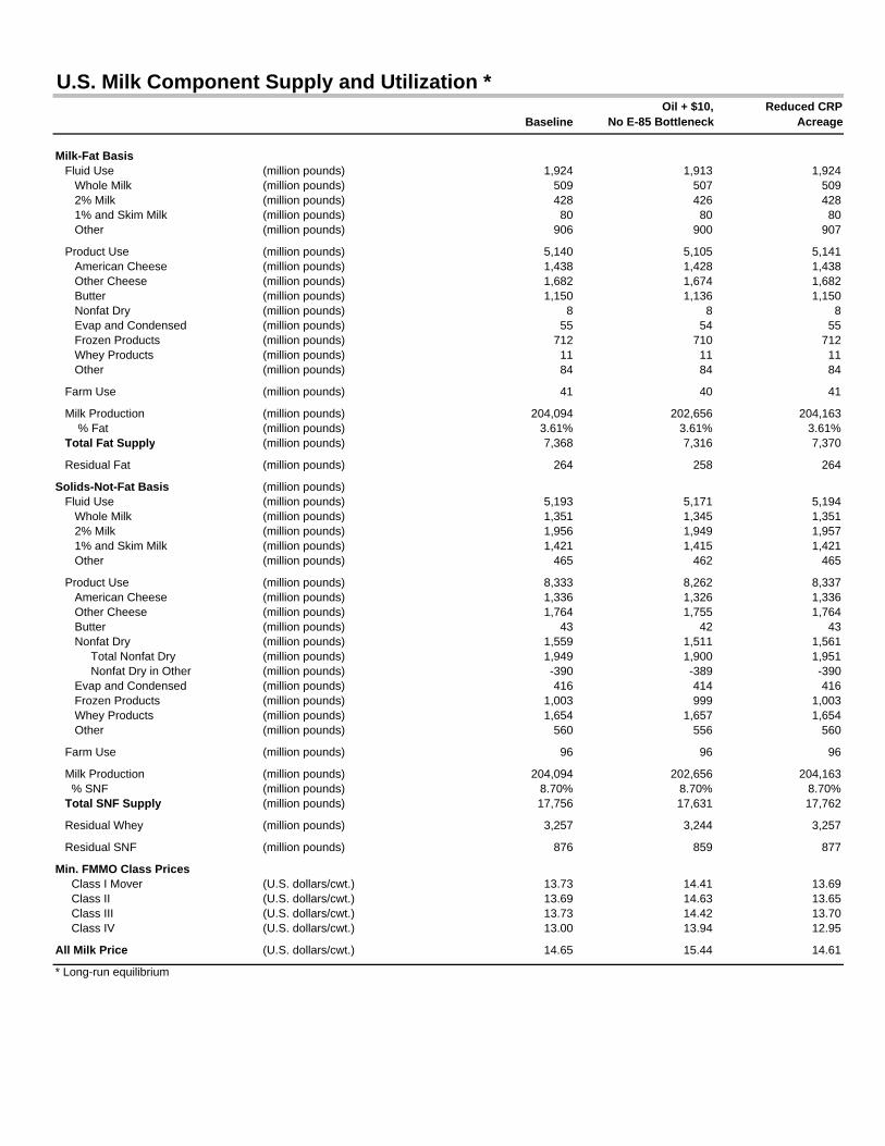
U.S. Milk Component Supply and Utilization *
BaselineOil + $10,
No E-85 BottleneckReduced CRP
Acreage
Milk-Fat Basis Fluid Use (million pounds) 1,924 1,913 1,924 Whole Milk (million pounds) 509 507 509 2% Milk (million pounds) 428 426 428 1% and Skim Milk (million pounds) 80 80 80 Other (million pounds) 906 900 907
Product Use (million pounds) 5,140 5,105 5,141 American Cheese (million pounds) 1,438 1,428 1,438 Other Cheese (million pounds) 1,682 1,674 1,682 Butter (million pounds) 1,150 1,136 1,150 Nonfat Dry (million pounds) 8 8 8 Evap and Condensed (million pounds) 55 54 55 Frozen Products (million pounds) 712 710 712 Whey Products (million pounds) 11 11 11 Other (million pounds) 84 84 84
Farm Use (million pounds) 41 40 41
Milk Production (million pounds) 204,094 202,656 204,163 % Fat (million pounds) 3.61% 3.61% 3.61% Total Fat Supply (million pounds) 7,368 7,316 7,370
Residual Fat (million pounds) 264 258 264
Solids-Not-Fat Basis (million pounds) Fluid Use (million pounds) 5,193 5,171 5,194 Whole Milk (million pounds) 1,351 1,345 1,351 2% Milk (million pounds) 1,956 1,949 1,957 1% and Skim Milk (million pounds) 1,421 1,415 1,421 Other (million pounds) 465 462 465
Product Use (million pounds) 8,333 8,262 8,337 American Cheese (million pounds) 1,336 1,326 1,336 Other Cheese (million pounds) 1,764 1,755 1,764 Butter (million pounds) 43 42 43 Nonfat Dry (million pounds) 1,559 1,511 1,561 Total Nonfat Dry (million pounds) 1,949 1,900 1,951 Nonfat Dry in Other (million pounds) -390 -389 -390 Evap and Condensed (million pounds) 416 414 416 Frozen Products (million pounds) 1,003 999 1,003 Whey Products (million pounds) 1,654 1,657 1,654 Other (million pounds) 560 556 560
Farm Use (million pounds) 96 96 96
Milk Production (million pounds) 204,094 202,656 204,163 % SNF (million pounds) 8.70% 8.70% 8.70% Total SNF Supply (million pounds) 17,756 17,631 17,762
Residual Whey (million pounds) 3,257 3,244 3,257
Residual SNF (million pounds) 876 859 877
Min. FMMO Class Prices Class I Mover (U.S. dollars/cwt.) 13.73 14.41 13.69 Class II (U.S. dollars/cwt.) 13.69 14.63 13.65 Class III (U.S. dollars/cwt.) 13.73 14.42 13.70 Class IV (U.S. dollars/cwt.) 13.00 13.94 12.95
All Milk Price (U.S. dollars/cwt.) 14.65 15.44 14.61
* Long-run equilibrium
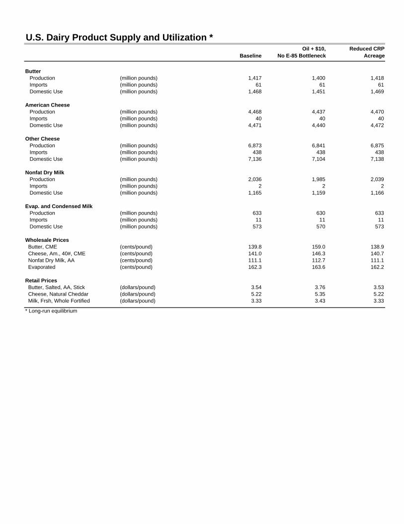
U.S. Dairy Product Supply and Utilization *
BaselineOil + $10,
No E-85 BottleneckReduced CRP
Acreage
Butter Production (million pounds) 1,417 1,400 1,418 Imports (million pounds) 61 61 61 Domestic Use (million pounds) 1,468 1,451 1,469
American Cheese Production (million pounds) 4,468 4,437 4,470 Imports (million pounds) 40 40 40 Domestic Use (million pounds) 4,471 4,440 4,472
Other Cheese Production (million pounds) 6,873 6,841 6,875 Imports (million pounds) 438 438 438 Domestic Use (million pounds) 7,136 7,104 7,138
Nonfat Dry Milk Production (million pounds) 2,036 1,985 2,039 Imports (million pounds) 2 2 2 Domestic Use (million pounds) 1,165 1,159 1,166
Evap. and Condensed Milk Production (million pounds) 633 630 633 Imports (million pounds) 11 11 11 Domestic Use (million pounds) 573 570 573
Wholesale Prices Butter, CME (cents/pound) 139.8 159.0 138.9 Cheese, Am., 40#, CME (cents/pound) 141.0 146.3 140.7 Nonfat Dry Milk, AA (cents/pound) 111.1 112.7 111.1 Evaporated (cents/pound) 162.3 163.6 162.2
Retail Prices Butter, Salted, AA, Stick (dollars/pound) 3.54 3.76 3.53 Cheese, Natural Cheddar (dollars/pound) 5.22 5.35 5.22 Milk, Frsh, Whole Fortified (dollars/pound) 3.33 3.43 3.33
* Long-run equilibrium