Emerging and Disappearing Work, Thriving and

Declining Firms

Enghin Atalay Sarada∗

May 7, 2020

Abstract

We propose a new measure of firms’ technology adoption, based on the types of

employees they seek. We construct firm-year level measures of emerging and disap-

pearing work using ads posted between 1940 and 2000 in the Boston Globe, New York

Times, and Wall Street Journal. Among the set of publicly listed firms, those which

post ads for emerging work tend to be younger, more R&D intensive, and have higher

future sales growth. Among all firms, those which post ads for emerging work are more

likely survive and, for privately held firms, are more likely to go public in the future.

We develop a model — consistent with these patterns —with incumbent job vintage

upgrading and firm entry and exit. Our estimated model indicates that 55 percent

of upgrading occurs through the entry margin, with incumbents accounting for the

remaining 45 percent.

1 Introduction

How do new technologies displace old ones? This is a foundational question in the fields

of economic growth, innovation, and management. At the firm level, the decision to adopt

a new technology in lieu of an existing one is risky, but with potentially high rewards. In

the aggregate, early adopters provide informational spillovers, paving the path for broad

adoption and productivity enhancements.

∗Atalay: Federal Reserve Bank of Philadelphia; Sarada: Department of Management and Human Re-sources, Wisconsin School of Business. We thank Sara Moreira and Sebastian Sotelo for helpful discussionsthroughout the early stages of this project. This work is being supported (in part) by Grant #92-18-05 fromthe Russell Sage Foundation. Research results and conclusions expressed are those of the authors and donot necessarily reflect the views of the Federal Reserve Bank of Philadelphia, the Federal Reserve System,or the Federal Reserve Board of Governors.

1

Unfortunately, comprehensive economy-wide firm-level measures of technology adop-

tion have been diffi cult to come by.1 In this paper, we provide a new angle to measuring

the types of technologies that firms utilize. We hypothesize that technologies are embedded

in work practices, namely in the types of workers and skills for which firms hire. We use

data on firms’job postings to learn about the technologies they are adopting, then assess

the sources of new technology adoption.

As we will demonstrate, there is substantial churn in the types of work performed

within and across firms. To provide one example, in the mid-twentieth century the Typist job

title was one of the most frequently occurring titles in the United States labor market. By the

1980s, typewriters were almost completely phased out of the workplace and few jobs carried

the Typist title. Instead, around this time, job titles like Word Processor were newly emerg-

ing. Other technology-specific or function-specific jobs titles like Comptometer Operator,

Stenographer, and Soda Dispenser were also once common but have since disappeared. Con-

versely, certain jobs which were common at the close of the twentieth century– including

Paralegal, LAN Administrator, and Systems Analyst– were virtually unknown fifty years

earlier. Each of these newly emerging job tittle is associated with a new technology —some

combination of techniques, processes, and administrative activities involved in the produc-

tion of goods and services —which firms adopt.

In this paper, we ask: What are the sources of this churn, this creative destruction?

Specifically, to what extent do new firms account for industries’technology upgrading? We

begin our study by constructing new measures of the vintages of work that firms seek in

their employees. Our measures are built using job ads posted in the Boston Globe, New York

Times, and Wall Street Journal over the 1940-2000 period. For each ad, we retrieve the job

title; and, for each job title we introduce measures of its relative newness. The intent of our

job vintage measures is to capture how “new”or “old”a job title is relative to the date at

which it is being hired for, with the broader goal of inferring the vintage of the technology

that firms utilize. Take the example from before of the Comptometer Operator job title.

While relatively common in the 1940s through 1960s, this job title had disappeared by 1980.

Thus, a firm hiring for a Comptometer Operator in 1940 may have been ahead of its time

in hiring for such work, while a firm doing the same thing in the 1970s would be hiring for

outmoded work. More generally, the “newness”of a job title corresponds to various qualities

that are typically indicative of technologies that are close to the frontier.2

1We discuss previous attempts at measurement in Section 2.2As Lin (2011) writes: “new job titles represent new combinations of activities or techniques that have

emerged in the labor market in response to the application of new information, technologies, or ‘recipes’toproduction.”(p. 554) We validate our measure of job title vintages in three ways. First, we demonstrate thatour job title vintage measures align with those developed in Lin (2011). Second, we show that newer vintage

2

We next document that firms with new or emerging job titles are more innovative

and better performing than firms posting ads for old or disappearing job titles. Among

publicly traded firms, those posting vacancies pertaining to new work have higher future

sales growth and are more R&D intensive: A one standard deviation increase in our job

title vintage measure corresponds to 4 percent faster sales growth over the next five years, 6

percent faster sales growth over the next ten years, and R&D expenditures to sales ratios that

are (among the sample of firms with positive R&D expenditures) higher by 11 log points.

Among all firms, those posting ads with newer vintage job titles are more likely to be publicly

traded and have (somewhat) more highly cited patents. Finally, young firms post ads for

newer vintage work, while firms that post ads for soon-to-be disappearing job titles are more

likely to exit the in the near future. While, reassuringly, our new job-title-based measure

of firm innovativeness correlates with existing measure, a key advantage to our measure is

that can be constructed for any firm that posts job ads, and is not limited to publicly traded

firms or to industries in which patenting is prevalent.3

Having established that our job title vintage measure relates to firm outcomes in

consequential and sensible ways, we apply our measure to quantify the extent to which

new firms account for technology upgrading. To do so, we construct a model of the two

sources of technology upgrading, either through firm entry and exit or through incumbents

investing in updating the technology vintage they employ. In our model, we assume that

consumers’ tastes shift as time progresses: Consumers prefer to purchase only varieties

produced by technologies suffi ciently close to the frontier. Firms with obsolete technologies,

by assumption, exit the industry. To maintain their position in the market, incumbents

forego current-period profits to (probabilistically) by incurring the cost to upgrade to the

frontier technology.4 In addition to incumbent firms technology upgrading, upgrading may

occur through the entry of new firms: They pay a sunk entry cost to enter with a relatively-

new technology vintage. Beyond technology vintages, firms differ in their age (the date at

which they first entered the economy) and their total factor productivity (exogenously given,

jobs tend to have higher posted salaries and have college degree requirements more frequently. And, third,newer vintage jobs more frequently require that prospective employees be familiar with new information andcommunication technologies. In other words, job title vintages have practical and meaningful implicationsfor the type of work firms are hiring for, and for the technological intensity of that work.

3Patenting is heavily concentrated in a small number of industries. These differences reflect not onlydifferences in industries’innovativeness but also differences across products in the extent to which patentsconfer intellectual property protection. As Argente, Baslandze, Hanley, and Moreira (2020) report in theirstudy of the consumer packaged good sector, many new product introducts are not associated with patentfilings.

4In reality, the obsolescence that induces firm exit may reflect not only changing consumer tastes, but alsothe introduction of newer, lower-cost technologies. The key features of our setup are that new technologiesexogenously appear, that firms face a costly decision of whether to adapt to the new technology, and thatlack of new technology adoption for a suffi ciently long period of time leads to firm exit.

3

determined upon entry).

According to our model, higher fixed entry costs (relative to the cost of incumbent

technology upgrading) implies that the value of having a frontier technology is high, which

in turn corresponds to a high benefit that incumbents accrue from technology upgrading.

With higher fixed entry costs, there are many high productivity firms who both survive to

be long-lived and have the newest vintage job titles. In the cross-section, older firms have

frontier technologies. And with high fixed costs, there is substantially more dispersion in

firms’ages than in technology vintages. In contrast, small fixed entry costs correspond to a

correlation between age and distance to the frontier that is close to 1 and similar levels of

dispersion in firm ages and job title vintages.

We estimate our model via a simulated method of moments procedure using data

on firms’ages, job vintages, and sales. We find that approximately 55 percent of technology

upgrading occurs through the entry margin when firms are weighted according to their sales,

more than 90 percent when firms are weighted equally. That is to say, both entry and

exit and incumbents costly investments are important channels of new technology adoption.

Finally, we explore heterogeneity across industries in the relative importance of the entry

margin. In manufacturing, where firms tend to be younger, on average, the net entry margin

accounts for a higher fraction of technology upgrading.

The remainder of our paper is structured as follows. Section 2 relates our work to the

recent literature within economics and management on innovative activity, macroeconomics

and labor economics. Section 3 then discusses the source data, our measurement of job title

vintages, and the correlates of emerging and disappearing work at the ad level. Section

4 characterizes the types of firms which post emerging and disappearing work. Section 5

develops and estimates our model of technology upgrading. Section 6 concludes.5

2 Related Literature

Our paper builds on and contributes to at least three interconnecting literatures within

economics: one which decomposes the sources of innovation between entrants and incum-

bents, one which studies the diffusion of new technologies, and one which uses job titles to

learn about technological change.

Regarding the first of these literatures, building on Klette and Kortum (2004), a

recent literature has evaluated the role that entrants play in propelling technological progress

5In the appendices, we outline our measurement of posted salaries, the identity of the posting firm, andjob titles (Appendix A), assess the representativeness of our sample, (Appendix B), present supplementaryempirical analyses (Appendix C), and discuss the simulation of our model (Appendix D).

4

through Schumpeterian product innovation; see, also, the review article by Aghion, Akcigit,

and Howitt (2014). More recently, Akcigit and Kerr (2018) and Garcia-Macia, Hsieh, and

Klenow (2019) each construct and estimate models whereby both entrants and incumbents

can engage in product – and, in Garcia-Macia, Hsieh, and Klenow (2019), process –

innovation. Both find that entrants account for approximately one-quarter of aggregate

productivity growth; see Table 6 of Akcigit and Kerr (2018) and Table 5 of Garcia-Macia,

Hsieh, and Klenow (2019). We also consider a model in which entrants and incumbents

account for technological change. The scope of our analysis is narrower than that in Akcigit

and Kerr (2018) and Garcia-Macia, Hsieh, and Klenow (2019): We are not seeking to provide

a comprehensive decomposition of aggregate TFP growth,only to understand the replacement

of old work practices for new ones. The advantage of this narrow scope is that it allows us

to focus on the type of technical change we can most directly measure: the vintages of

technologies that firms adopt.

Our work also relates to a voluminous work on the introduction and diffusion of new

technologies. Empirical works either examine industry or aggregate data on the adoption

rates of a wide variety of new technologies (Gort and Klepper (1982); Comin and Hobijn

(2004, 2010); Anzoategui, Comin, Gertler, and Martinez (2019)); or examines the firm-

or individual-level adoption rates of a single or handful of technologies (Henderson and

Clark (1990); Conley and Udry (2010)). Papers that develop models consistent with this

literature include Jovanovic and Lach (1989), Chari and Hopenhayn (1991), Jovanovic and

MacDonald (1994), and Jovanovic and Yatsenko (2012). Relative to the empirical portion of

the literature on technology diffusion, our firm-level measures are comparable across a wide

swath technologies and industries. Relative to the theoretical portion, our contribution is to

develop a heterogeneous firm model in which both the net entry and incumbent upgrading

margin can play a role.6

We are not the first to propose the use of job titles in the study of innovation. In his

work on the agglomeration of innovation, Lin (2011) creatively proposes the use of job titles

to identify new work within the census occupation classification system. This allows him

to classify new job titles, as they appear over long horizons. In more recent work, Atalay,

Phongthiengtham, Sotelo, and Tannenbaum (2020) compare new versus old job titles and

their task content. We find that, even within similar occupational groups, newer job titles

are more non-routine task intensive. Relative to these papers, the key novelty in our work

is to link firms to the vintage of job titles in their vacancies.7

6Among the cited papers, only Jovanovic and Lach (1989) contains technology upgrading through firmentry and exit. In their paper, firms are homogeneous within each cohort and cannot upgrading the vintageof their capital after they enter.

7Like us, Deming and Kahn (2018) relate firm characteristics to the content in their job ads. They find

5

In sum, our paper makes two key advances over the existing literature. First, we

introduce newmeasures of technology adoption at the firm-year level, over a long time horizon

and across a wide swath of firms. Second, we develop a model of technology adoption to

answer a new substantive question.

3 Data and Measurement Issues

3.1 Data Source and Variables

Our dataset is drawn from ads which were originally published in the Boston Globe, New

York Times, and Wall Street Journal. Atalay, Phongthiengtham, Sotelo, and Tannenbaum

(2018, 2020) outline the algorithm for transforming the unprocessed newspaper text into

a structured database. There, we describe how to extract, from each vacancy posting,

information on the ad’s job title, the tasks which the worker is expected to perform, and the

technologies that the worker uses on the job. We also delineate how we assign a Standard

Occupation Classification (SOC) code to each job title.8 The dataset contains 9.26 million

ads from 1940 to 2000. In this paper, our focus is on the dates at which each job title –

already extracted in our previous work – appears in our newspaper text. Since our measures

of job title emergence and disappearance are computed based on the distribution of dates

in which the job title appeared, we restrict attention to job titles which appear suffi ciently

frequently, in at least 20 distinct ads through the sample period. With this restriction, the

benchmark dataset contains 5.21 million job ads.

New to this paper, whenever possible we attempt to retrieve the firm or employment

agency which placed the ad, as well as the job’s posted salary. To recover information on

the posting party, we search for certain string types that tend to appear in conjunction with

that firms posting ads containing a greater frequency of mentions of social and cognitive skills also tendto pay higher wages, have higher labor productivity, and are more likely to be publicly traded. Demingand Noray (2019) explore emerging and disappearing work, not through ads’job titles but instead throughskill requirements mentioned in the ads’bodies. For each occupation, they measure the extent to whichskill requirements change over time. They find that the life-cycle wage profile is flatter in fast-changingoccupations, in particular in STEM-related jobs.

8The main task categories correspond to measures explored by Spitz-Oener (2006): nonroutine analytic,nonroutine interactive, and nonroutine manual tasks; and routine cognitive and routine manual tasks. Atalay,Phongthiengtham, Sotelo, and Tannenbaum (2020) describes the full set of job ad words which correspondto each of these five task groups. The 48 technologies include offi ce ICTs (e.g., Microsoft Excel, MicrosoftPowerPoint, Microsoft Word, WordPerfect), hardware (e.g., IBM 360, IBM 370), general purpose software(e.g., C++, FORTRAN, Java); see Atalay, Phongthiengtham, Sotelo, and Tannenbaum (2018) for a fulllist of the technologies. The Standard Occupation Classification is an occupational classification systemdeveloped by the United States government. By assigning an SOC code to each job title, one may link ourdatabase of job ads’task and technology mentions to surveys developed and maintained by governmentalagencies (e.g., the American Community Survey).

6

the name of a firm: “agency,”“agcy,”“associate,”“associates,”“assoc,”“co,”“company,”

“corp,” “corporation,” “inc,” “incorporated,” “llc,” and “personnel.” We also search for

instances of a 7-digit number (which would indicate a phone number), or a set of strings

which would indicate an address of the posting firm. When these string types occur, we

examine the surrounding words, and then manually group common firms. As much as

possible, we consistently record firms’identities, even in cases in which naming conventions

differ within the sample period.

Among the 5.21 million ads which will form the basis for the analysis, below, we

could extract information on the posting party for 712 thousand ads. For these 712 thousand

ads, we could identify only a phone number or address for 163 thousand ads. For 296

thousand ads, the posting party we identified was an employment agency. For the remaining

252 thousand ads, we have identified an employer who is placing the ad on its own behalf.

Among these, for 205 thousand ads, we have identified the firm’s 2-digit industry code, and

the entry date for 195 thousand ads.9 We could match the identity of the posting party

to the Compustat dataset in 82 thousand ads, and to the NBER Patenting database for

38 thousand ads. Finally, to retrieve information on the posted salary, we again search for

groups of strings that tend to reflect a person’s salary. Among the 5.21 million ads that form

the base sample, we could extract information on the posted salary for 190 thousand ads.

Appendix A provides additional information on algorithms with which we group job titles,

identify posted salaries, and identify the firm or employment agency which is posting the job

ad. In the same appendix, we also illustrate the performance of these algorithms through an

example page of ads. In Appendix B, we examine the extent to which the ads for which we

can identify the employer is representative of the broader sample of newspaper job ads.

3.2 Measuring Job Title Vintages

For each job title j, we compute a triple of statistics, summarizing the dates at which

the job title was introduced to and disappeared from our dataset. Quoting from our earlier

work, we “define vpj , vintages of job title j, as the pth quantile of the distribution of years

in which the job title appears in our data. In computing these quantiles, for each job title,

we weight according to the job title’s share of ads (Sjt) in each year. For p close to 0, vpjcompares different job titles based on when they first emerged in our data set. In contrast, vpjfor p close to 1 compares job titles based on their disappearance from our dataset.”(Atalay,

Phongthiengtham, Sotelo, and Tannenbaum (2020), p. 29) Our main analysis centers around

v0.01j as our measure for the year in which job title j entered the dataset, v0.99j as our measure

9We have identified these pieces of information through manual online searches.

7

for year in which job title j left the dataset, and v0.50j as capturing the average vintage of

job title j.10

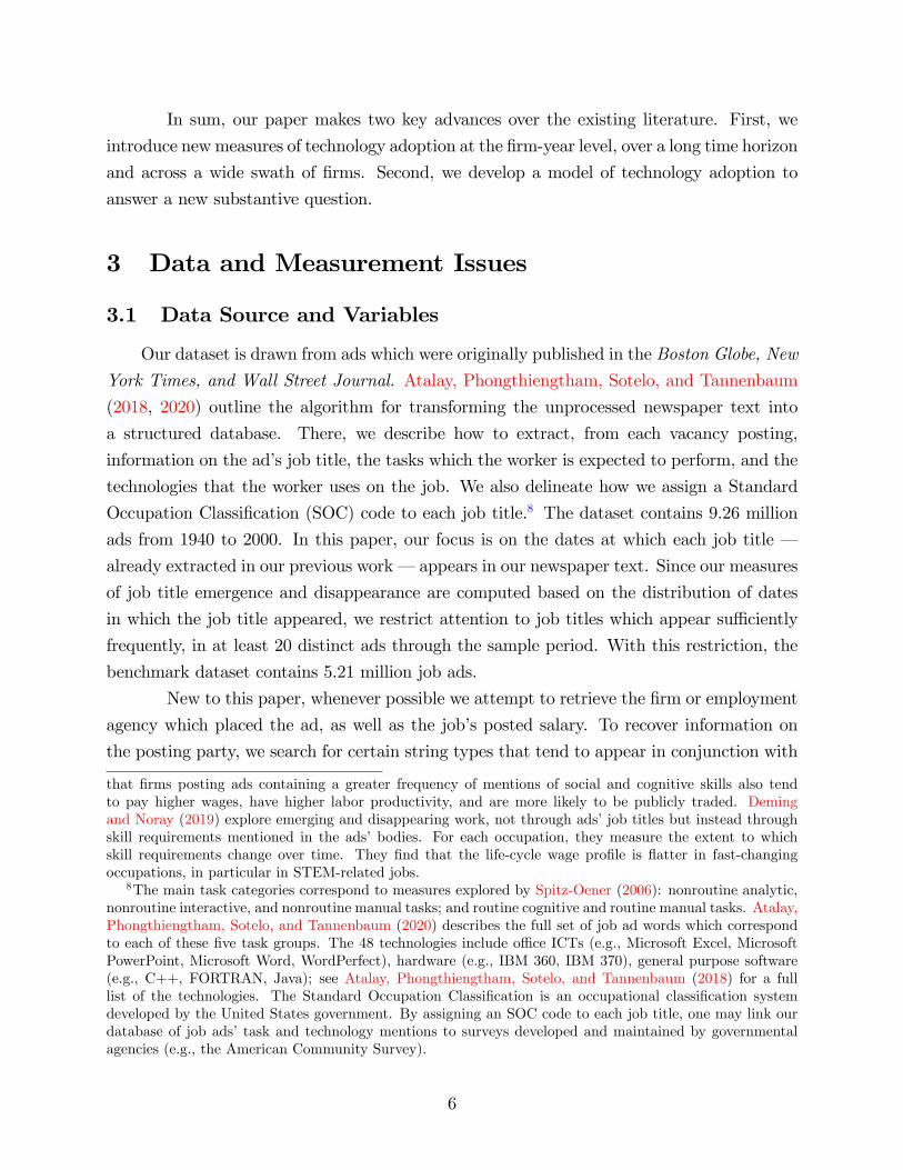
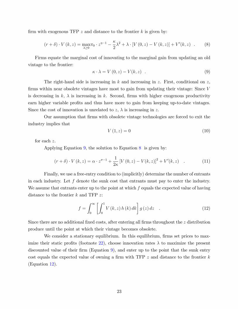
Figure 1 illustrates the construction of these percentiles for two job titles. There, we

plot the share of ads for which the job title equals Figure Clerk or Comptometer Operator.

These are two job titles for different types of financial clerical work. At its peak, in the

late 1940s and early 1950s, approximately 0.2 to 0.3 percent of all ads within the newspaper

data were for Comptometer Operators. By 1970, few if any job ads were for a Comptometer

Operator position. On the other hand, Figure Clerk was rarely mentioned in the 1940s.

Then, beginning in the 1950s there was a slow, steady increase in the number of job ads for

which Figure Clerk was the job title. To depict the time-span over which each of these two

job titles were in use, we plot three vertical lines. For the Comptometer Operator job title,

the 1st, 50th, and 99th percentile years in which the title was mentioned are 1941, 1952, and

1974. In other words,(v0.01j , v0.50j , v0.99j

)= (1941, 1952, 1974) for j =Comptometer Operator.

Analogously, for j =Figure Clerk v0.01j = 1950, v0.50j = 1970, and v0.99j = 1988.

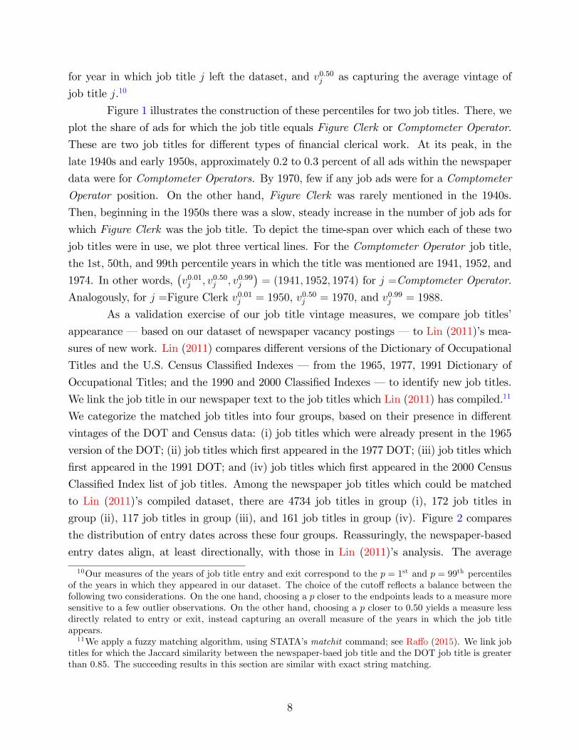
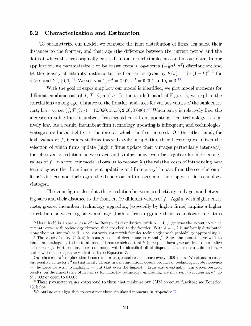
As a validation exercise of our job title vintage measures, we compare job titles’

appearance – based on our dataset of newspaper vacancy postings – to Lin (2011)’s mea-

sures of new work. Lin (2011) compares different versions of the Dictionary of Occupational

Titles and the U.S. Census Classified Indexes – from the 1965, 1977, 1991 Dictionary of

Occupational Titles; and the 1990 and 2000 Classified Indexes – to identify new job titles.

We link the job title in our newspaper text to the job titles which Lin (2011) has compiled.11

We categorize the matched job titles into four groups, based on their presence in different

vintages of the DOT and Census data: (i) job titles which were already present in the 1965

version of the DOT; (ii) job titles which first appeared in the 1977 DOT; (iii) job titles which

first appeared in the 1991 DOT; and (iv) job titles which first appeared in the 2000 Census

Classified Index list of job titles. Among the newspaper job titles which could be matched

to Lin (2011)’s compiled dataset, there are 4734 job titles in group (i), 172 job titles in

group (ii), 117 job titles in group (iii), and 161 job titles in group (iv). Figure 2 compares

the distribution of entry dates across these four groups. Reassuringly, the newspaper-based

entry dates align, at least directionally, with those in Lin (2011)’s analysis. The average

10Our measures of the years of job title entry and exit correspond to the p = 1st and p = 99th percentilesof the years in which they appeared in our dataset. The choice of the cutoff reflects a balance between thefollowing two considerations. On the one hand, choosing a p closer to the endpoints leads to a measure moresensitive to a few outlier observations. On the other hand, choosing a p closer to 0.50 yields a measure lessdirectly related to entry or exit, instead capturing an overall measure of the years in which the job titleappears.11We apply a fuzzy matching algorithm, using STATA’s matchit command; see Raffo (2015). We link job

titles for which the Jaccard similarity between the newspaper-baed job title and the DOT job title is greaterthan 0.85. The succeeding results in this section are similar with exact string matching.

8

0.0

01.0

02.0

03Fr

eque

ncy 

of A

ds o

f Ads

1940 1950 1960 1970 1980 1990 2000Year

Figure Clerk Comptometer Operator

Figure 1: Job title frequencies.Notes: We plot the frequency of two individual job titles for each year between 1940 and 2000. The verticallines depict v0.01j , v0.50j , and v0.99j for each of the two titles. The smoothed lines are computed using a localpolynomial smoother. Within the 1940 to 2000 sample, there were 4544 ads for Figure Clerks and 5772 adsfor Comptometer Operators.

entering vintage of newspaper job titles in group (i) is 4.4 years earlier than in group (ii), 9.2

years earlier than in group (iii), and 11.1 years earlier than in group (iv).12 However, there

are a substantial number of group (iii) and (iv) job titles – job titles which first appear

in either the 1991 DOT list or the 2000 Census Classified Index – which were present in

early-year newspaper job ads. For instance, the Assistant Buyer, General Superintendent,

and Portrait Photographer job titles all first appeared in the 2000 Census Classified Index,

but had 10 percent of their newspaper job ads appear before 1965.

3.3 Characteristics of Emerging and Disappearing Work

Before exploring the relationship between ads’job title vintages and characteristics of

the firms that post these ads, we establish three characteristics of emerging and disappearing

work. First, for vacancy postings in which the employer posts a salary, newer jobs have on

average higher posted salaries. Second, newer vintage jobs tend to also include mentions

of new technologies. And, third, job ads corresponding to newer vintage jobs also include

degree (either bachelors or graduate) requirements. To emphasize, these three relationships

12In these averages, each job title is weighted equally. Weighting job titles by the number of times theyappear in our dataset, the three differences – between group (i) versus groups (ii), (iii), and (iv) – are 4.0years, 5.6 years, and 8.7 years, respectively.

9

0.0

2.0

4.0

6.0

8D

ensi

ty

1940 1960 1980 2000Vintage, 1st Percentile

Present in 1965 Enter after 1965, by 1977Enter after 1977, by 1991 Enter after 1991, by 2000

Figure 2: Density of entry dates.Notes: This figure presents the density of entry dates, as measured within the newspaper vacancy postings,for four groups of job titles. The four groups are based on the dates in which they first appear within theDictionary of Occupational Titles or the Census Classified Index.

should be afforded a descriptive, not causal, interpretation. The goal of these exercises is to

illustrate that new and disappearing job titles are, respectively, meaningfully different from

existing and surviving job titles. New job titles reflect a reorganization of production toward

innovative, skill-complementing techniques.

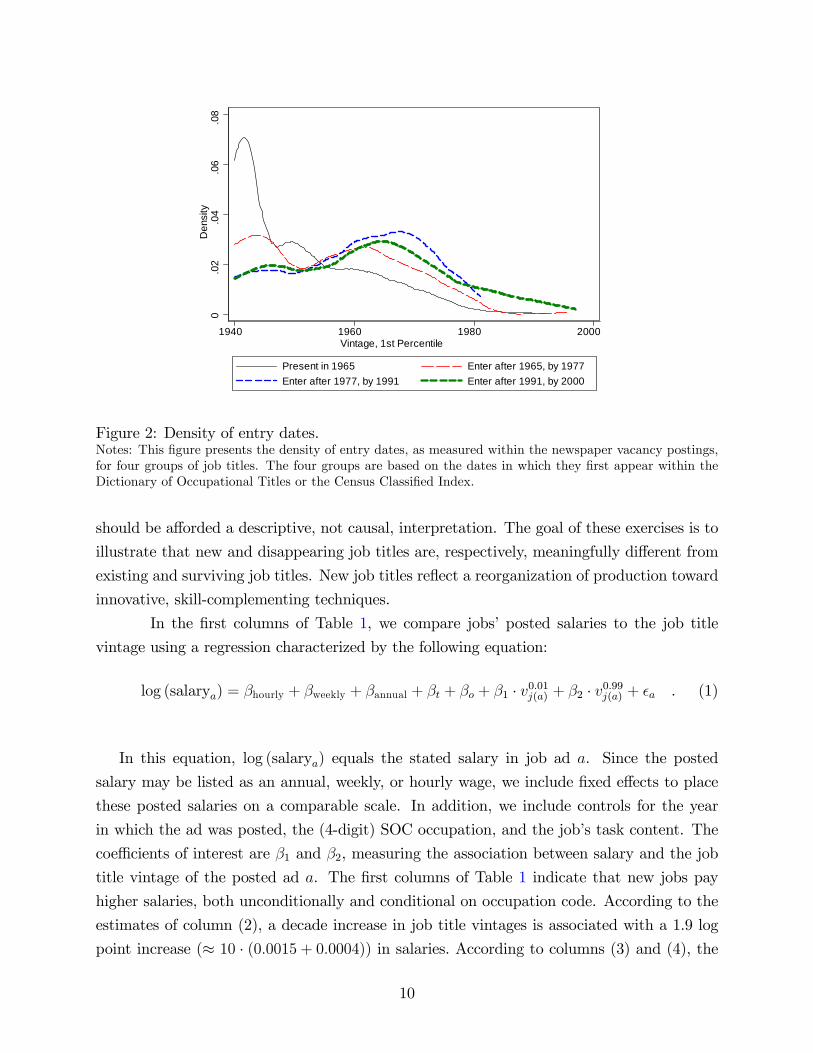
In the first columns of Table 1, we compare jobs’posted salaries to the job title

vintage using a regression characterized by the following equation:

log (salarya) = βhourly + βweekly + βannual + βt + βo + β1 · v0.01j(a) + β2 · v0.99j(a) + εa . (1)

In this equation, log (salarya) equals the stated salary in job ad a. Since the posted

salary may be listed as an annual, weekly, or hourly wage, we include fixed effects to place

these posted salaries on a comparable scale. In addition, we include controls for the year

in which the ad was posted, the (4-digit) SOC occupation, and the job’s task content. The

coeffi cients of interest are β1 and β2, measuring the association between salary and the job

title vintage of the posted ad a. The first columns of Table 1 indicate that new jobs pay

higher salaries, both unconditionally and conditional on occupation code. According to the

estimates of column (2), a decade increase in job title vintages is associated with a 1.9 log

point increase (≈ 10 · (0.0015 + 0.0004)) in salaries. According to columns (3) and (4), the

10

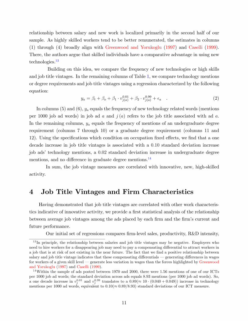
relationship between salary and new work is localized primarily in the second half of our

sample. As highly skilled workers tend to be better remunerated, the estimates in columns

(1) through (4) broadly align with Greenwood and Yorukoglu (1997) and Caselli (1999).

There, the authors argue that skilled individuals have a comparative advantage in using new

technologies.13

Building on this idea, we compare the frequency of new technologies or high skills

and job title vintages. In the remaining columns of Table 1, we compare technology mentions

or degree requirements and job title vintages using a regression characterized by the following

equation:

ya = βt + βo + β1 · v0.01j(a) + β2 · v0.99j(a) + εa . (2)

In columns (5) and (6), ya equals the frequency of new technology related words (mentions

per 1000 job ad words) in job ad a and j (a) refers to the job title associated with ad a.

In the remaining columns, ya equals the frequency of mentions of an undergraduate degree

requirement (columns 7 through 10) or a graduate degree requirement (columns 11 and

12). Using the specifications which condition on occupation fixed effects, we find that a one

decade increase in job title vintages is associated with a 0.10 standard deviation increase

job ads’technology mentions, a 0.02 standard deviation increase in undergraduate degree

mentions, and no difference in graduate degree mentions.14

In sum, the job vintage measures are correlated with innovative, new, high-skilled

activity.

4 Job Title Vintages and Firm Characteristics

Having demonstrated that job title vintages are correlated with other work characteris-

tics indicative of innovative activity, we provide a first statistical analysis of the relationship

between average job vintages among the ads placed by each firm and the firm’s current and

future performance.

Our initial set of regressions compares firm-level sales, productivity, R&D intensity,

13In principle, the relationship between salaries and job title vintages may be negative. Employers whoneed to hire workers for a disappearing job may need to pay a compensating differential to attract workers ina job that is at risk of not existing in the near future. The fact that we find a positive relationship betweensalary and job title vintage indicates that these compensating differentials – generating differences in wagesfor workers of a given skill level – generate less variation in wages than the forces highlighted by Greenwoodand Yorukoglu (1997) and Caselli (1999).14Within the sample of ads posted between 1970 and 2000, there were 1.56 mentions of one of our ICTs

per 1000 job ad words; the standard deviation across ads equals 8.93 mentions (per 1000 job ad words). So,a one decade increase in v0.01j and v0.99j translates to a 0.89(≈ 10 · (0.040 + 0.049)) increase in technologymentions per 1000 ad words, equivalent to 0.10(≈ 0.89/8.93) standard deviations of our ICT measure.

11

(1) (2) (3) (4) (5) (6)Dep. Variable – – – – – — Log Salary – – – – – — TechnologyYear 0.0018 0.0015 0.0003 0.0020 0.106 0.040of Emergence (0.0002) (0.0002) (0.0004) (0.0002) (0.001) (0.001)Year 0.0026 0.0004 -0.0003 0.0034 0.078 0.049of Disappearance (0.0002) (0.0002) (0.0003) (0.0004) (0.001) (0.001)Mean of Dep. Variable 1.56Std. Dev. of Dep. Variable 0.64 0.52 1.11 8.93N (thousand) 180 97 84 2,174SOC F.E. No Yes Yes Yes No YesSample 1940-2000 1940-1969 – – 1970-2000 – –

(7) (8) (9) (10) (11) (12)Dep. Variable – – Undergraduate Degree – – Graduate DegreeYear 0.0118 0.0063 0.0106 0.0060 -0.0028 -0.0077of Emergence (0.0003) (0.0003) (0.0008) (0.0004) (0.0005) (0.0005)Year 0.0074 0.0033 0.0038 0.0062 0.0327 0.0100of Disappearance (0.0002) (0.0003) (0.0003) (0.0007) (0.0004) (0.0004)Mean of Dep. Variable 0.56 0.44 0.73 1.66Std. Dev. of Dep. Variable 4.14 3.70 4.64 7.62N (thousand) 5,043 2870 2174 5,043SOC F.E. No Yes Yes Yes No YesSample 1940-2000 1940-1969 1970-2000 1940-2000

Table 1: Relationship between job title vintages, salaries, technology measures, and educa-tional requirements.Notes: The coeffi cient estimates and standard errors in columns (1) through (4) correspond to estimationsof Equation 1. The coeffi cient estimates and standard errors in columns (5) through (12) correspond toestimations of Equation 2. SOC F.E. refers to fixed effects for the 4-digit SOC of each ad.

12

future sales growth, and future productivity growth to measures of job title vintages. For

the ads that a firm i places in year t, we average over the job vintage measures that we

introduced in the previous section:

Avg. Year of Emergenceit =1

|Ait|·∑a∈Ait

v0.01j(a) , (3)

Avg. Median Yearit =1

|Ait|·∑a∈Ait

v0.50j(a) , and (4)

Avg. Year of Disappearanceit =1

|Ait|·∑a∈Ait

v0.99j(a) . (5)

In these equations, Ait refers to the set of ads that firm posted in year t and |Ait| to thenumber of ads within this set.

Our comparisons are based on the following regression specification:

xit = βt + β1 ·Avg. Year of Emergenceit + β2 ·Avg. Median Yearit (6)

+ β3 ·Avg. Year of Disappearanceit + γ ·Xit + εit .

Within Equation 6, xit represents either firm-year level labor productivity, R&D intensity,

future sales growth, or labor productivity growth; βt are year-level fixed effects; and, Xit

are firm-level controls. These include the the logarithm of the firm’s book value of total

assets, employment, and revenues in year t; the fraction of the firm’s ads that are in each

2-digit occupation code in year t; and 1-digit industry-level fixed effects. The coeffi cients

of interest, β1, β2, and β3, thus characterize the relationship between firms’propensity to

post ads for emerging and disappearing job titles on the one hand, and productivity, R&D

intensity, and future sales and productivity growth on the other hand. To emphasize, by

including year-level fixed effects (βt), our comparisons between job title vintages and other

firm characteristics exploit variation across firms within a given year. Throughout this

section, we weight observations by the number of job ads posted by firm i in year t.15

Table 2 presents the results from this exercise. Here, the sample includes the set of

firm-year observations for which the name of the posting firm could be matched to a firm in

the Compustat database and where the firm was publicly traded in the year during which

the ad was posted. The first four columns of Table 2 suggest that there is a weak, positive

relationship between firms’revenues and their job title vintages. According to column (2),

15Most, but not all, of the results presented in this section are similar in unweighted specifications. Wehighlight differences when they occur, below. Appendix C.2 collects the analogues of Tables 2 to 6 whereobservations are weighted equally.

13

for example, a 3.74 year increase job title vintages (equivalent to the across-firm, within-year

standard deviation of the job title vintage measure) is associated with a 7 percent increase in

sales. The relationship between vintage and revenues is no longer statistically significant once

one controls for the shares of firm-year job ads that are posted in each 2-digit occupation code

(column 4).16 Columns (5) through (8) assess the relationships among job vintages and labor

productivity. For the most part, the relationship between job title vintage and productivity is

not statistically significant. Columns (9) through (16) indicate that there is stark increasing

relationship between firms’job vintage measures and R&D intensity. Among the set of firms

with positive R&D expenditures, a one-standard deviation increase in job title vintages is

associated with a 11 percent increase in R&D intensity (column 10). Among the broader set

of firms, an equivalent increase in job title vintages is associated with R&D intensity that

is 58 log points higher (column 14). Controlling for both industry and occupational mix

attenuates these estimated relationships for broader of firms (compare column 14 to column

16) but not for firms with positive R&D expenditures (compare columns 10 and 12). In sum,

Table 2 suggests, first, that firms posting for newer vintage work are (perhaps) somewhat

more productive and larger, and that, second, newer vintage job titles are correlated with

R&D intensity.

So, Table 2 indicates that new work practices are a marker of innovative activity. Is

our job title vintage measure, then, predictive of future firm outcomes? Table 3 addresses

this question. In the first eight columns, we relate firms’job posting behavior in year t to

their sales growth up to year t+ 5 (columns 1 through 4) or year t+ 10 (columns 5 through

8). Across all specifications, firms that post ads for newer vintage jobs grow faster. A one

standard deviation increase in our Avg. Median Yearijt measure corresponds to 4 percent

faster growth over the next five years, 6 percent over the next decade. (While the regressions

in Table 3 omit R&D intensity as a covariate, the results would be nearly unchanged with

this variable’s inclusion.) In these first eight columns, our sample includes only firms that

survive up to five years (in the first four columns) or ten years (columns 5 through 8). Since

omission from the sample largely corresponds to firms that have poor outcomes, the first

eight columns likely understate the relationship between growth and job title vintages. In

columns (9) through (16), we account for this sample selection problem. Here, we show that

the association between sales growth and job title vintages is stronger (columns 9 through

12) and that firms posting for newer work practices also tend to experience an increase in

labor productivity (columns 13 through 16).

16In unweighted specifications, firms that post ads for older vintage job titles are larger and more pro-ductive. However, with the exception of the estimate of β1 in the specification corresponding to column (3),these relationships are not statistically significant.

14

(1)

(2)

(3)

(4)

(5)

(6)

(7)

(8)

Dep.Variable

–––

log

(yit)

–––

––

log

(lp it)

––

Avg.Yearof

0.006

-0.0002

Emergence it

(0.012)

(0.0020)

Avg.Median

0.032

0.018

-0.014

0.0003

0.0011

—0.0021

Year it

(0.009)(0.009)

(0.009)

(0.0020)

(0.0017)

(0.0020)

Avg.Yearof

0.011

0.0123

Disappearanceit

(0.015)

(0.0043)

OtherControls

None

IndustryF.E.

IndustryF.E.

SOCShares

None

IndustryF.E.

IndustryF.E.

SOCShares

R2

0.088

0.142

0.185

0.185

0.815

0.863

0.868

0.867

(9)

(10)

(11)

(12)

(13)

(14)

(15)

(16)

Dep.Variable

––

log

(R&Dit/y

it)

––

––

log

(R&Dit/y

it)

––

Avg.Yearof

0.033

0.032

Emergence it

(0.007)

(0.034)

Avg.Median

0.041

0.030

0.031

0.264

0.154

0.055

Year it

(0.007)(0.006)

(0.006)

(0.039)

(0.035)

(0.034)

Avg.Yearof

0.004

-0.083

Disappearanceit

(0.011)

(0.064)

OtherControls

None

IndustryF.E.

IndustryF.E.

SOCShares

None

IndustryF.E.

IndustryF.E.

SOCShares

R2

0.261

0.340

0.375

0.376

0.300

0.418

0.442

0.441

Table2:Relationshipbetweenjobtitlevintage,sales,productivity,andR&Dintensity.

Notes:The“SOCShares”refertovariableswhichmeasuretheshareofads,withinthefirm-yearobservation,correspondingtoeach2-digitSOC

code.Theemployment,sales,assets,andR&Ddataarecomputedusingdatafrom

Compustat.Incolumns(5)-(16),theregressionsalsoinclude

log(assets)andlog(employment)ascovariates.Incolumns(9)-(12),onlyfirm-yearobservationswithpositiveR&Dexpendituresareincluded.In

columns(13)-(16),weimputemissinglog(R&Dtosalesratios)usingtheminimum

valueinoursample.Thesampleincolumns(1)-(4)includes5005

firm-yearobservationscorrespondingto81thousandjobads;thesampleincolumns(5)-(8)and(13)-(16)includes4830observations,corresponding

to78thousandjobads;thesampleincolumns(9)-(12)includes2520observations,correspondingto38thousandjobads.

15

(1)

(2)

(3)

(4)

(5)

(6)

(7)

(8)

Dep.Variable

––––

log

(yi,t+5/y

it)

–––

––

log

(yi,t+10/y

it)

––

Avg.Yearof

0.006

0.012

Emergence it

(0.003)

(0.004)

Avg.Median

0.013

0.010

0.008

0.020

0.016

0.014

Year it

(0.002)(0.002)

(0.002)

(0.004)(0.003)

(0.003)

Avg.Yearof

0.002

0.002

Disappearanceit

(0.003)

(0.004)

OtherControls

None

IndustryF.E.

IndustryF.E.

SOCShares

None

IndustryF.E.

IndustryF.E.

SOCShares

R2

0.206

0.241

0.247

0.250

0.225

0.261

0.273

0.276

(9)

(10)

(11)

(12)

(13)

(14)

(15)

(16)

Dep.Variable

–––

log

(yi,t+10/y

it)

––

–––

log

(lp i,t+10/lp it)

––

Avg.Yearof

0.024

0.016

Emergence it

(0.006)

(0.005)

Avg.Median

0.040

0.026

0.019

0.022

0.013

0.012

Year it

(0.004)(0.004)

(0.005)

(0.004)(0.004)

(0.004)

Avg.Yearof

0.007

0.005

Disappearanceit

(0.006)

(0.006)

OtherControls

None

IndustryF.E.

IndustryF.E.

SOCShares

None

IndustryF.E.

IndustryF.E.

SOCShares

R2

0.054

0.066

0.068

0.068

0.054

0.066

0.068

0.068

Table3:Relationshipbetweenjobtitlevintage,salesgrowth,andlaborproductivitygrowth.

Notes:The“SOCShares”refertovariableswhichmeasuretheshareofads,withinthefirm-yearobservation,correspondingtoeach2-digitSOCcode.

Theemployment,sales,andassetdataarecomputedusingdatafrom

Compustat.Ineachregression,log(assets)andlog(employment)areincluded

ascovariates.Incolumns(1)-(8)thesampleincludesonlyfirm-yearobservationswhicharepresentintheCompustatdatabasefiveortenyearslater.

Incolumns(9)-(16),weestimateacensored(Tobit)regression,imputingthevalueforsalesandlaborproductivitygrowthtobeequalto−

2forfirms

thatexittheCompustatsample,andsettingthelowerthresholdatthispoint.Thesampleincolumns(1)-(4)includes4368firm-yearobservations,

correspondingto75thousandjobads.Thesampleincolumns(5)-(8)includes3897firm-yearobservations,correspondingto71thousandjobads.

Thesampleincolumns(9)-(16)includes4830fim-yearobservations,correspondingto78thousandjobads.

16

(1) (2) (3) (4) (5) (6)

Dep. Variable Publicly TradedPublicly Traded Within

10 Years?Avg. Year of 0.0067 0.0072Emergenceit (0.0019) (0.0021)Avg. Median 0.0128 0.0053 0.0033 0.0042Yearit (0.0015) (0.0016) (0.0015) (0.0014)Avg. Year of 0.0043 0.0021Disappearanceit (0.0025) (0.0019)

Other Controls Industry F.E.Industry F.E.SOC Shares

Industry F.E.Industry F.E.SOC Shares

R2 0.219 0.248 0.248 0.127 0.137 0.136

Table 4: Relationship between job title vintage and firms’publicly traded status.Notes: The “SOC Shares”refer to variables which measure the share of ads, within the firm-year observation,corresponding to each 2-digit SOC code. Within columns (4)-(6), the dependent variable “Publicly Tradedwithin 10 Years”is an indicator variable, equal to 1 if the posting firm can be matched to a publicly tadedfirm in the Compustat database, entering the database within 10 years of the ad’s posting. Within thesecolumns, the sample includes observations for which the firm has not entered the Compustat database at thetime of the ad’s posting. The sample in columns (1)-(3) includes 14257 firm-year observations, correspondingto 205 thousand job ads. The sample in columns (4)-(6) includes 8770 firm-year observations, correspondingto 121 thousand ads.

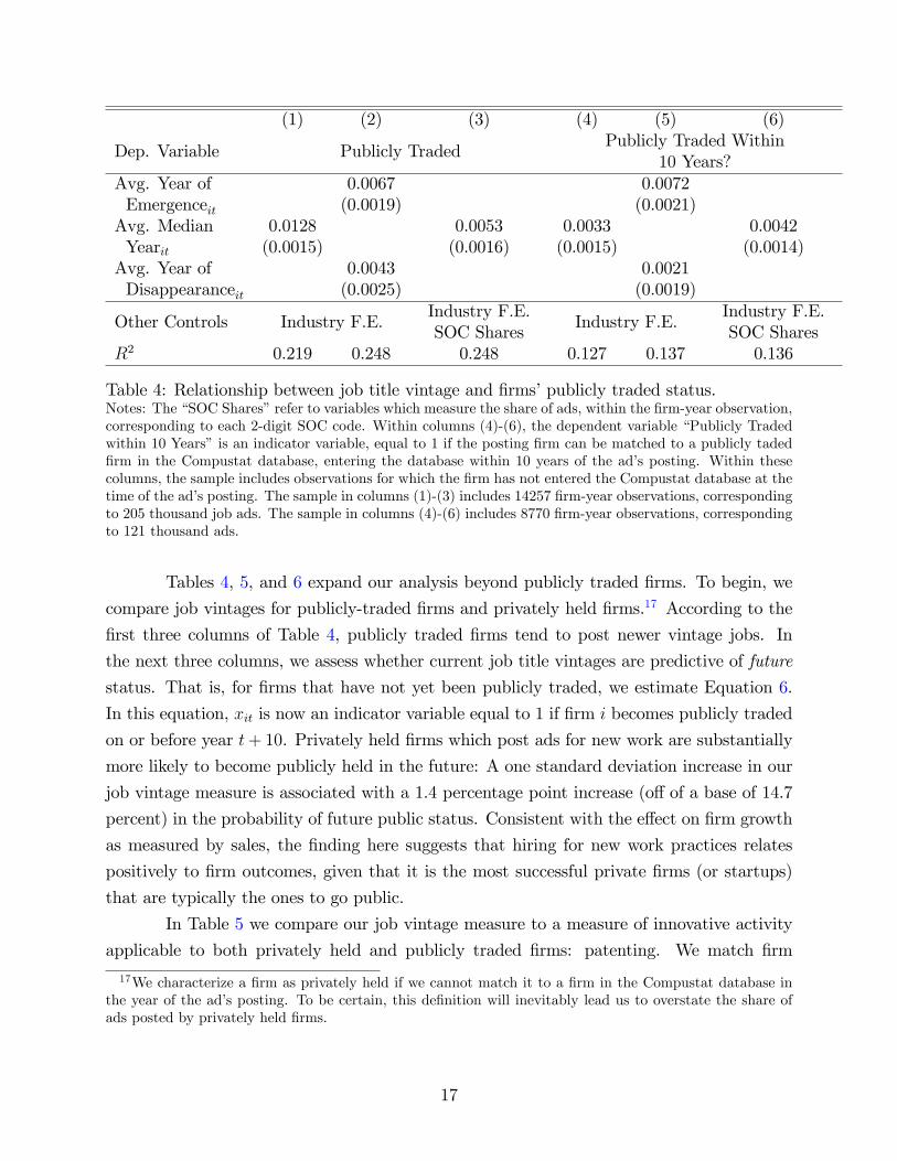
Tables 4, 5, and 6 expand our analysis beyond publicly traded firms. To begin, we

compare job vintages for publicly-traded firms and privately held firms.17 According to the

first three columns of Table 4, publicly traded firms tend to post newer vintage jobs. In

the next three columns, we assess whether current job title vintages are predictive of future

status. That is, for firms that have not yet been publicly traded, we estimate Equation 6.

In this equation, xit is now an indicator variable equal to 1 if firm i becomes publicly traded

on or before year t+ 10. Privately held firms which post ads for new work are substantially

more likely to become publicly held in the future: A one standard deviation increase in our

job vintage measure is associated with a 1.4 percentage point increase (off of a base of 14.7

percent) in the probability of future public status. Consistent with the effect on firm growth

as measured by sales, the finding here suggests that hiring for new work practices relates

positively to firm outcomes, given that it is the most successful private firms (or startups)

that are typically the ones to go public.

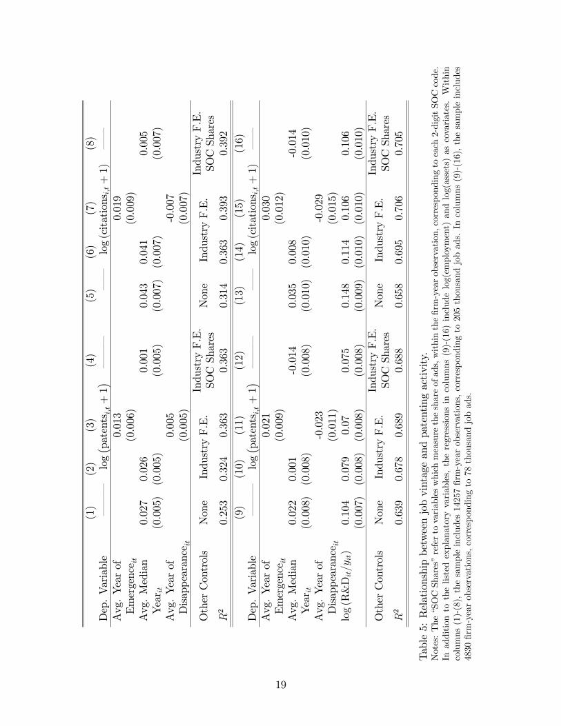
In Table 5 we compare our job vintage measure to a measure of innovative activity

applicable to both privately held and publicly traded firms: patenting. We match firm

17We characterize a firm as privately held if we cannot match it to a firm in the Compustat database inthe year of the ad’s posting. To be certain, this definition will inevitably lead us to overstate the share ofads posted by privately held firms.

17

names in our newspaper dataset to those in the NBER Patenting Database.18 According

to this table, firms that post ads with newer vintage job titles tend patent more frequently

(columns 1-4) and have patents that are more patent citations (columns 5-8). In the final

eight columns of Table 5, we assess the relationship between patenting and job vintages,

now conditioning on R&D intensity. In part because the sample is now restricted to publicly

traded firms, the estimated relationships in columns (9) to (16) are substantially weaker

than those in columns (1) to (8). In sum, firms with more patents and more highly cited

patents post ads for newer vintage work, but this relationship potentially reflects underlying

differences in firms’R&D intensity and in industry composition.

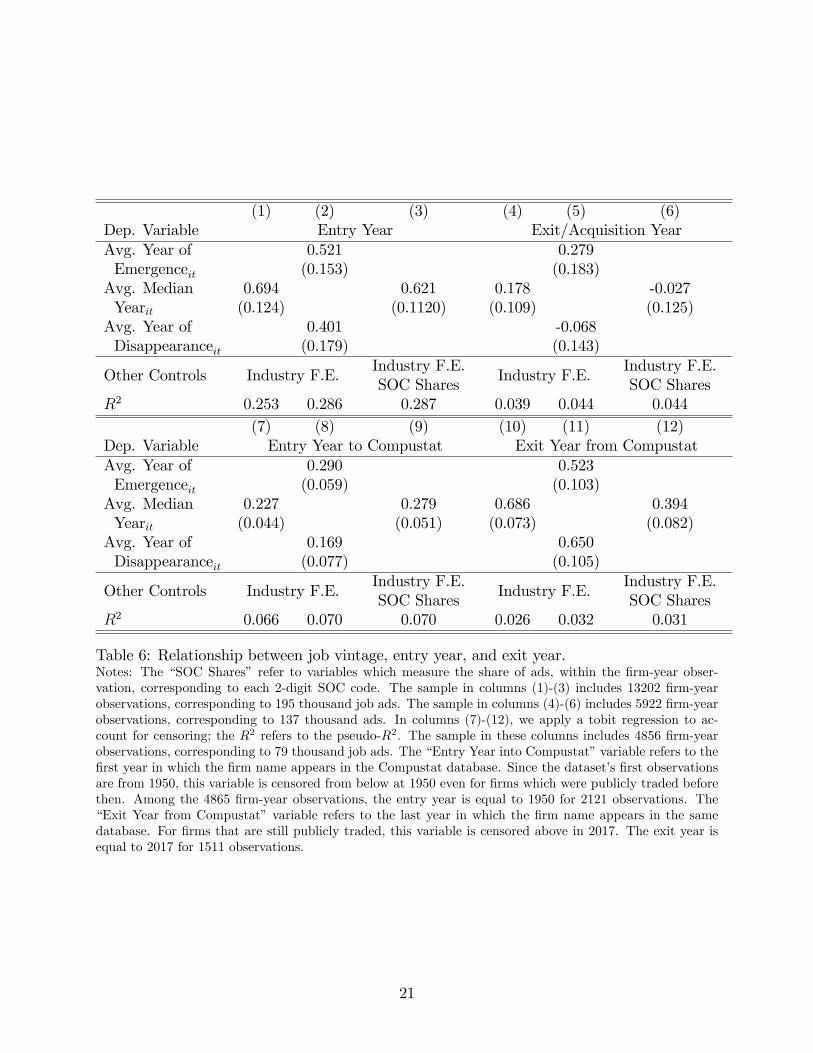
Do younger firms post ads for newer work practices? And does posting ads for soon-

to-be disappearing jobs predict exit from the market? Table 6 compares firms’cohorts with

the job title vintages that they post. To do so, we apply the regression specification given

in Equation 6, with the dependent variable equal to year in which the firm first entered,

or exited from, the market. (To emphasize, since we are controlling for the year in which

the ad is posted, the relationships that are identified are not mechanically reflecting the

passage of time within our sample.) We apply two differing measures of entry and exit,

each with their own advantages and disadvantages. In the first six columns, our measures

of entry and exit are collected from hand web searching, while in the final six columns our

entry and exit measure capture appearance or disappearance from publicly traded status

(measured as presence or absence in the Compustat database). The hand-collected data

have the advantage of capturing true entry and exit – not simply entry and exit from

publicly traded status – and span a wider set of firms, but have the disadvantage of relying

on our own judgement in certain instances.19 Columns (1) and (4) indicate that firms with

one-decade newer job title vintages tend to be younger by 6.9 years (column 1 of Table 6) and

survive for an additional 1.8 years (column 4), though the latter estimate is not significantly

different from zero. In terms of entry to or exit from publicly traded status (columns 7

through 12), the results are somewhat weaker for the date of entry and somewhat stronger

18We use the database that covers patenting activity between 1963 and 1999, downloaded fromhttps://data.nber.org/patents/pat63_99.txt.For firms that we could not find a name match, we set the patent or citation counts to be equal to zero,

assuming that the reason that the lack of the match reflects no actual patenting activity by the firm that isposting the job ad. The results in Table 5 are similar when restricting to firm-year observations for whichwe could match firm names across the newspaper and NBER patenting databases.19There are at least two complications in assigning a date of exit. First, struggling firms tend to be

acquired (at, potentially, a price much lower than the book value of its assets) as opposed to shutting downcompletely. We treat being acquired as exit from the market, but acknowledge that this choice is open todebate. Second, struggling firms will declare bankruptcy, potentially reorganizing at the same point in time,but then continue under the same name. We treat these events as also exiting from the industry, againrealizing that alternate choices may also be defensible.

18

(1)

(2)

(3)

(4)

(5)

(6)

(7)

(8)

Dep.Variable

–––

log( pat

entsi,t+

1)–––

––

log

(citations

i,t+

1)––

Avg.Yearof

0.013

0.019

Emergence it

(0.006)

(0.009)

Avg.Median

0.027

0.026

0.001

0.043

0.041

0.005

Year it

(0.005)(0.005)

(0.005)

(0.007)(0.007)

(0.007)

Avg.Yearof

0.005

-0.007

Disappearanceit

(0.005)

(0.007)

OtherControls

None

IndustryF.E.

IndustryF.E.

SOCShares

None

IndustryF.E.

IndustryF.E.

SOCShares

R2

0.253

0.324

0.363

0.363

0.314

0.363

0.393

0.392

(9)

(10)

(11)

(12)

(13)

(14)

(15)

(16)

Dep.Variable

–––

log( pat

entsi,t+

1)–––

––

log

(citations

i,t+

1)––

Avg.Yearof

0.021

0.030

Emergence it

(0.009)

(0.012)

Avg.Median

0.022

0.001

-0.014

0.035

0.008

-0.014

Year it

(0.008)(0.008)

(0.008)

(0.010)(0.010)

(0.010)

Avg.Yearof

-0.023

-0.029

Disappearanceit

(0.011)

(0.015)

log

(R&Dit/y

it)

0.104

0.079

0.07

0.075

0.148

0.114

0.106

0.106

(0.007)(0.008)(0.008)

(0.008)

(0.009)(0.010)(0.010)

(0.010)

OtherControls

None

IndustryF.E.

IndustryF.E.

SOCShares

None

IndustryF.E.

IndustryF.E.

SOCShares

R2

0.639

0.678

0.689

0.688

0.658

0.695

0.706

0.705

Table5:Relationshipbetweenjobvintageandpatentingactivity.

Notes:The“SOCShares”refertovariableswhichmeasuretheshareofads,withinthefirm-yearobservation,correspondingtoeach2-digitSOCcode.

Inadditiontothelistedexplanatoryvariables,theregressionsincolumns(9)-(16)includelog(employment)andlog(assets)ascovariates.Within

columns(1)-(8),thesampleincludes14257firm-yearobservations,correspondingto205thousandjobads.Incolumns(9)-(16),thesampleincludes

4830firm-yearobservations,correspondingto78thousandjobads.

19

for the date of exit.

To sum up, while firms which post ads for newer vintage jobs are only slightly (if

at all) larger and more productive contemporaneously, they are more innovative and have

faster growth in the future. To arrive at this conclusion, we compare publicly traded firms’

job vintage to their R&D intensity, to future sales growth, and to the year in which the firm

entered and exited from the universe of publicly traded firms. We then show that – among

privately-held firms – firms that post newer vintage jobs are more likely to be publicly

traded in the future.20

5 A Model of Technology Upgrading

We consider a model of technology upgrading and obsolescence consistent with the pat-

terns documented in the previous section. In our economy, there are two margins through

which technologies of different vintages evolve: entrants (who, on average, posses newer

vintage technologies) replacing exiting firms, and incumbent firms upgrading their technolo-

gies. Within our framework, technology upgrading is necessary to keep pace with consumers’

evolving preferences.21 The goal of our model is to use the joint distribution of firms’ages,

their technology vintages, and their revenues to infer the relative costs of entry and incum-

bent technology upgrading.

5.1 Setup

Consider a continuous time economy, where time is indexed by t. Each firm i produces

a single variety. There is a representative consumer who has preferences over the different

varieties consumed:

Uτ =

∫ ∞τ

e−r(t−τ) log (Ct) dt , where

Ct =

[∫i:v(i)∈[t,t+1]

ct (i)(η−1)/η di

]η/(η−1).

20Complementing these exercises, in Appendix C.3 we illustrate through narrative examples the relation-ship between firm performance and job title vintages. We compare DEC and Wang Laboratories – twofirms which, in the 1960s and 1970s respectively advertised for newly emerging work – to American Biltrite,and Bethlehem Steel – two firms which sought out employees to perform jobs which were soon to disappear.21An alternate formulation with similar observable implications would involve (i) new technologies ap-

pearing that, once adopted, allow firms to produce at a reduced marginal cost, and (ii) overhead costs ofproduction. As in our model, firms which fail to update their technology eventually would be eventuallyforced to exit the industry.

20

(1) (2) (3) (4) (5) (6)Dep. Variable Entry Year Exit/Acquisition YearAvg. Year of 0.521 0.279Emergenceit (0.153) (0.183)Avg. Median 0.694 0.621 0.178 -0.027Yearit (0.124) (0.1120) (0.109) (0.125)Avg. Year of 0.401 -0.068Disappearanceit (0.179) (0.143)

Other Controls Industry F.E.Industry F.E.SOC Shares

Industry F.E.Industry F.E.SOC Shares

R2 0.253 0.286 0.287 0.039 0.044 0.044(7) (8) (9) (10) (11) (12)

Dep. Variable Entry Year to Compustat Exit Year from CompustatAvg. Year of 0.290 0.523Emergenceit (0.059) (0.103)Avg. Median 0.227 0.279 0.686 0.394Yearit (0.044) (0.051) (0.073) (0.082)Avg. Year of 0.169 0.650Disappearanceit (0.077) (0.105)

Other Controls Industry F.E.Industry F.E.SOC Shares

Industry F.E.Industry F.E.SOC Shares

R2 0.066 0.070 0.070 0.026 0.032 0.031

Table 6: Relationship between job vintage, entry year, and exit year.Notes: The “SOC Shares” refer to variables which measure the share of ads, within the firm-year obser-vation, corresponding to each 2-digit SOC code. The sample in columns (1)-(3) includes 13202 firm-yearobservations, corresponding to 195 thousand job ads. The sample in columns (4)-(6) includes 5922 firm-yearobservations, corresponding to 137 thousand ads. In columns (7)-(12), we apply a tobit regression to ac-count for censoring; the R2 refers to the pseudo-R2. The sample in these columns includes 4856 firm-yearobservations, corresponding to 79 thousand job ads. The “Entry Year into Compustat”variable refers to thefirst year in which the firm name appears in the Compustat database. Since the dataset’s first observationsare from 1950, this variable is censored from below at 1950 even for firms which were publicly traded beforethen. Among the 4865 firm-year observations, the entry year is equal to 1950 for 2121 observations. The“Exit Year from Compustat” variable refers to the last year in which the firm name appears in the samedatabase. For firms that are still publicly traded, this variable is censored above in 2017. The exit year isequal to 2017 for 1511 observations.

21

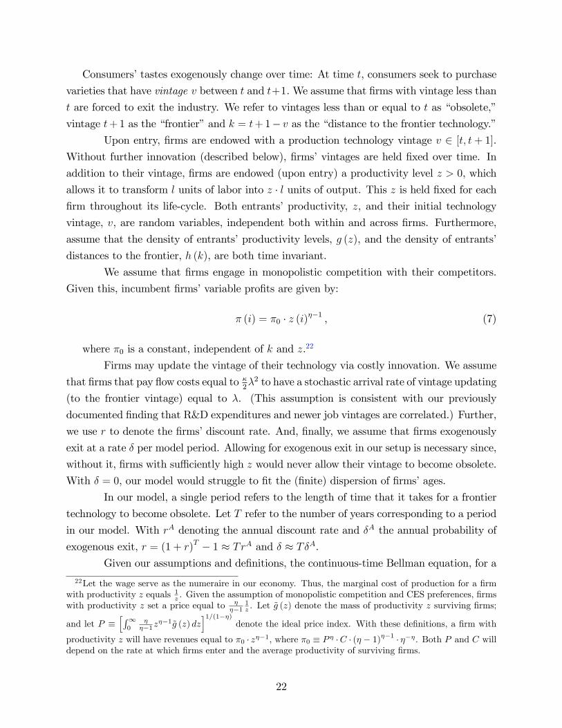
Consumers’tastes exogenously change over time: At time t, consumers seek to purchase

varieties that have vintage v between t and t+1.We assume that firms with vintage less than

t are forced to exit the industry. We refer to vintages less than or equal to t as “obsolete,”

vintage t+ 1 as the “frontier”and k = t+ 1− v as the “distance to the frontier technology.”Upon entry, firms are endowed with a production technology vintage v ∈ [t, t+ 1].

Without further innovation (described below), firms’vintages are held fixed over time. In

addition to their vintage, firms are endowed (upon entry) a productivity level z > 0, which

allows it to transform l units of labor into z · l units of output. This z is held fixed for eachfirm throughout its life-cycle. Both entrants’productivity, z, and their initial technology

vintage, v, are random variables, independent both within and across firms. Furthermore,

assume that the density of entrants’productivity levels, g (z), and the density of entrants’

distances to the frontier, h (k), are both time invariant.

We assume that firms engage in monopolistic competition with their competitors.

Given this, incumbent firms’variable profits are given by:

π (i) = π0 · z (i)η−1 , (7)

where π0 is a constant, independent of k and z.22

Firms may update the vintage of their technology via costly innovation. We assume

that firms that pay flow costs equal to κ2λ2 to have a stochastic arrival rate of vintage updating

(to the frontier vintage) equal to λ. (This assumption is consistent with our previously

documented finding that R&D expenditures and newer job vintages are correlated.) Further,

we use r to denote the firms’discount rate. And, finally, we assume that firms exogenously

exit at a rate δ per model period. Allowing for exogenous exit in our setup is necessary since,

without it, firms with suffi ciently high z would never allow their vintage to become obsolete.

With δ = 0, our model would struggle to fit the (finite) dispersion of firms’ages.

In our model, a single period refers to the length of time that it takes for a frontier

technology to become obsolete. Let T refer to the number of years corresponding to a period

in our model. With rA denoting the annual discount rate and δA the annual probability of

exogenous exit, r = (1 + r)T − 1 ≈ TrA and δ ≈ TδA.

Given our assumptions and definitions, the continuous-time Bellman equation, for a

22Let the wage serve as the numeraire in our economy. Thus, the marginal cost of production for a firmwith productivity z equals 1z . Given the assumption of monopolistic competition and CES preferences, firmswith productivity z set a price equal to η

η−11z . Let g̃ (z) denote the mass of productivity z surviving firms;

and let P ≡[∫∞0

ηη−1z

η−1g̃ (z) dz]1/(1−η)

denote the ideal price index. With these definitions, a firm with

productivity z will have revenues equal to π0 · zη−1, where π0 ≡ P η ·C · (η − 1)η−1 · η−η. Both P and C will

depend on the rate at which firms enter and the average productivity of surviving firms.

22

firm with exogenous TFP z and distance to the frontier k is given by:

(r + δ) · V (k, z) = maxλ≥0

π0 · zη−1 −κ

2λ2 + λ · [V (0, z)− V (k, z)] + V ′(k, z) . (8)

Firms equate the marginal cost of innovating to the marginal gain from updating an old

vintage to the frontier:

κ · λ = V (0, z)− V (k, z) . (9)

The right-hand side is increasing in k and increasing in z. First, conditional on z,

firms within near obsolete vintages have most to gain from updating their vintage: Since V

is decreasing in k, λ is increasing in k. Second, firms with higher exogenous productivity

earn higher variable profits and thus have more to gain from keeping up-to-date vintages.

Since the cost of innovation is unrelated to z, λ is increasing in z.

Our assumption that firms with obsolete vintage technologies are forced to exit the

industry implies that

V (1, z) = 0 (10)

for each z.

Applying Equation 9, the solution to Equation 8 is given by:

(r + δ) · V (k, z) = α · zσ−1 +1

2κ[V (0, z)− V (k, z)]2 + V ′(k, z) . (11)

Finally, we use a free-entry condition to (implicitly) determine the number of entrants

in each industry. Let f denote the sunk cost that entrants must pay to enter the industry.

We assume that entrants enter up to the point at which f equals the expected value of having

distance to the frontier k and TFP z:

f =

∫ ∞0

[∫ 1

0

V (k, z)h (k) dk

]g (z) dz . (12)

Since there are no additional fixed costs, after entering all firms throughout the z distribution

produce until the point at which their vintage becomes obsolete.

We consider a stationary equilibrium. In this equilibrium, firms set prices to max-

imize their static profits (footnote 22), choose innovation rates λ to maximize the present

discounted value of their firm (Equation 9), and enter up to the point that the sunk entry

cost equals the expected value of owning a firm with TFP z and distance to the frontier k

(Equation 12).

23

5.2 Characterization and Estimation

To parameterize our model, we compare the joint distribution of firms’log sales, their

distances to the frontier, and their age (the difference between the current period and the

date at which the firm originally entered) in our model simulations and in our data. In our

application, we parameterize z to be drawn from a log-normal(−12σ2, σ2

)distribution; and

let the density of entrants’distance to the frontier be given by h (k) = β · (1− k)β−1 for

β ≥ 0 and k ∈ [0, 1].23 We set κ = 1, rA = 0.02, δA = 0.001 and η = 3.24

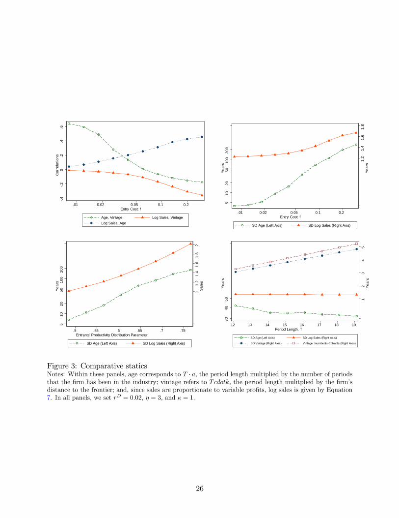
With the goal of explaining how our model is identified, we plot model moments for

different combinations of f , T , β, and σ. In the top left panel of Figure 3, we explore the

correlations among age, distance to the frontier, and sales for various values of the sunk entry

cost; here we set (f, T, β, σ) = (0.060, 15.10, 2.06, 0.606).25 When entry is relatively free, the

increase in value that incumbent firms would earn from updating their technology is rela-

tively low. As a result, incumbent firm technology updating is infrequent, and technologies’

vintages are linked tightly to the date at which the firm entered. On the other hand, for

high values of f , incumbent firms invest heavily in updating their technologies. Given the

selection of which firms update (high z firms update their vintages particularly intensely),

the observed correlation between age and vintage may even be negative for high enough

values of f . In short, our model allows us to recover κf(the relative costs of introducing new

technologies either from incumbent updating and from entry) in part from the correlation of

firms’vintages and their ages, the dispersion in firm ages and the dispersion in technology

vintages..

The same figure also plots the correlation between productivity and age, and between

log sales and their distance to the frontier, for different values of f . Again, with higher entry

costs, greater incumbent technology upgrading (especially by high z firms) implies a higher

correlation between log sales and age (high z firms upgrade their technologies and thus

23Here, h (k) is a special case of the Beta(α, β) distribution, with α = 1; β governs the extent to whichentrants enter with technology vintages that are close to the frontier. With β = 1, k is uniformly distributedalong the unit interval; as β →∞, entrants’enter with frontier technologies with probability approaching 1.24The value of entry V (0, z) is homogeneous of degree one in κ and f . Since the moments we wish to

match are orthogonal to the total mass of firms (which all that V (0, z) pins down), we are free to normalizeeither κ or f . Furthermore, since our model will be identified off of dispersion in firms variable profits, ηand σ will not be separately identified; see Equation 7.Our choice of δA implies that firms exit for exogenous reasons once every 1000 years. We choose a small

but positive value for δA so that nearly all exit in our simulations occurs because of technological obsolescence– the force we wish to highlight – but that even the highest z firms exit eventually. Our decompositionresults, on the importance of net entry for industry technology upgrading, are invariant to increasing δA upto 0.002 or down to 0.0005.25These parameter values correspond to those that minimize our SMM objective funciton; see Equation

13, below.We outline our algorithm to construct these simulated moments in Appendix D.

24

survive longer) and a more negative correlation between firms’log sales and their distance

to the frontier.

In the top right panel, we again vary f but plot the dispersion in firms’ages and

their sales. With higher f , greater incumbent technology updating entails longer survival

for certain firms, primarily high productivity firms. This implies greater dispersion in firms’

ages, and – since more high-productivity firms participate in the market – greater dis-

persion in firm sales. In the bottom left panel of Figure 3, we again depict dispersion in

firms’log sales and their ages, now varying the dispersion in entrants’productivity levels

Increases in σ mechanically translate to increases in firms’log sales. With more dispersion

in productivity,there is greater dispersion in the returns from technology updating, yielding

an increase in the dispersion in firms’ages. Overall, the dispersions of age and sales each

depend both f and σ, however with differing sensitivities.

Finally, and with the aim of communicating how T is identified, the bottom right

panel of Figure 3 plots various moments as functions of T . Mechanically, as T increases,

the standard deviation of firms’ages and their vintages increases. However, since increasing

the period length effectively increases firms’discount rate, with lower T incumbents engage

in more technology upgrading, leading to more longer-lived firms and thus to a more firm

age distribution. In sum, holding other parameters fixed, higher T is associated with more

dispersed firm vintages, and less dispersed firm ages.

We estimate f , T , β, and σ via a simulated method of moments procedure. Our

seven moments are the standard deviations (i) of firms’log sales, (ii) of firms’age, (iii) and

of firms’distance to the frontier; the correlations (iv) between firm log sales and age, (v)

between firm log sales and distance to the frontier, and (vi) between firm age and distance

to the frontier; and (vii) the average vintage of entrants (firms with age less than five years)

relative to all firms. Using Θ to denote the five-dimensional vector of parameters we are

trying to estimate, mD to denote the seven-dimensional vector of moments, and m (Θ) to

denote the simulated moments, our parameters minimize

(m (Θ)−mD

)·(ΣD)−1 · (m (Θ)−mD

)′. (13)

Within this equation, ΣD is the covariance matrix of our seven moments, which we

compute by resampling from our dataset from 250 times.

Table 7 presents the results of our estimation. According to our model estimates,

the length of time between the frontier technology and obsolete technologies are roughly

T = 15.10 years. Second, the estimate of β = 2.06 implies that entrants have, on average,

technologies that are roughly one-third(≈ 1

2.06+1

)of the way between frontier and obso-

25

­.4­.2

0.2

.4.6

Cor

rela

tions

.01 0.02 0.05 0.1 0.2Entry Cost: f

Age, Vintage Log Sales, VintageLog Sales, Age

1.2

1.4

1.6

1.8

Year

s

510

2050

100

200

Year

s

.01 0.02 0.05 0.1 0.2Entry Cost: f

SD Age (Left Axis) SD Log Sales (Right Axis)

11.

21.

41.

61.

82

Sale

s

510

2050

100

200

Year

s

.5 .55 .6 .65 .7 .75Entrants' Productivity Distribution Parameter

SD Age (Left Axis) SD Log Sales (Right Axis)

12

34

5Ye

ars

4030

50Ye

ars

12 13 14 15 16 17 18 19Period Length, T

SD Age (Left Axis) SD Log Sales (Right Axis)

SD Vintage (Right Axis) Vintage: Inumbents­Entrants (Right Axis)

Figure 3: Comparative staticsNotes: Within these panels, age corresponds to T · a, the period length multiplied by the number of periodsthat the firm has been in the industry; vintage refers to Tcdotk, the period length mulitplied by the firm’sdistance to the frontier; and, since sales are proportionate to variable profits, log sales is given by Equation7. In all panels, we set rD = 0.02, η = 3, and κ = 1.

26

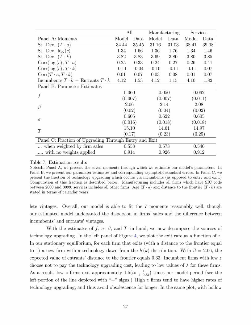
All Manufacturing ServicesPanel A: Moments Model Data Model Data Model DataSt. Dev. (T · a) 34.44 35.45 31.16 31.03 38.41 39.08St. Dev. log (c) 1.34 1.66 1.36 1.76 1.34 1.46St. Dev. (T · k) 3.82 3.83 3.69 3.80 3.80 3.85Corr(log (c) , T · a) 0.25 0.33 0.24 0.27 0.26 0.41Corr(log (c) , T · k) -0.11 -0.04 -0.10 -0.11 -0.11 0.07Corr(T · a, T · k) 0.01 0.07 0.03 0.08 0.01 0.07Incumbents T · k − Entrants T · k 4.12 1.53 4.12 1.15 4.10 1.82Panel B: Parameter Estimates

f0.060(0.007)

0.050(0.007)

0.062(0.011)

β2.06(0.02)

2.14(0.04)

2.08(0.02)

σ0.605(0.016)

0.622(0.018)

0.605(0.018)

T15.10(0.17)

14.61(0.23)

14.97(0.25)

Panel C: Fraction of Upgrading Through Entry and Exit... when weighted by firm sales 0.558 0.573 0.546.... with no weights applied 0.914 0.926 0.912

Table 7: Estimation resultsNotes:In Panel A, we present the seven moments through which we estimate our model’s parameters. InPanel B, we present our paramater estimates and corresponding asymptotic standard errors. In Panel C, wepresent the fraction of technology upgrading which occurs via incumbents (as opposed to entry and exit.)Computation of this fraction is described below. Manufacturing includes all firms which have SIC codebetween 2000 and 3999; services includes all other firms. Age (T · a) and distance to the frontier (T · k) arestated in terms of calendar years.

lete vintages. Overall, our model is able to fit the 7 moments reasonably well, though

our estimated model understated the dispersion in firms’sales and the difference between

incumbents’and entrants’vintages.

With the estimates of f , σ, β, and T in hand, we now decompose the sources of

technology upgrading. In the left panel of Figure 4, we plot the exit rate as a function of z.

In our stationary equilibrium, for each firm that exits (with a distance to the frontier equal

to 1) a new firm with a technology dawn from the h (k) distribution. With β = 2.06, the

expected value of entrants’distance to the frontier equals 0.33. Incumbent firms with low z

choose not to pay the technology upgrading cost, leading to low values of λ for these firms.

As a result, low z firms exit approximately 1.5(≈ 11−0.33) times per model period (see the

left portion of the line depicted with “+”signs.) High z firms tend to have higher rates of

technology upgrading, and thus avoid obsolescence for longer. In the same plot, with hollow

27

circles, we depict the rate of vintage upgrading that occurs through entry and exit.

Conversely, as the top right panel of Figure 4 illustrates, high z firms tend to update

their vintages more frequently than low z firms. For firms with z > 4.7, vintage upgrading

occurs at least once per model period (see the line depicted with “+”signs). Since technology

upgrading involves both firms with k close to 1 and those with k substantially less than 1

upgrading to the frontier technology, we must integrate over the possible values of k to

compute the rate at which new vintages replace old ones through incumbents’ innovation

decisions. The second line (depicted with hollow circles) within the figure’s top right panel

presents this.

Combining the results from the top two panels, the bottom left panel presents the

fraction of technology upgrading that occurs via entry and exit as opposed to incumbents’

upgrading. For firms with z < 3.5, vintage upgrading occurs primarily through entry and

exit; for high productivity firms the opposite is true.

In the bottom right panel, we plot the productivity distribution, both for incumbents

and for all firms. Since high productivity firms update their technologies more frequently,

relative to the entrants’productivity distribution (dashed line), there are more surviving

firms in the right tail. Integrating over the distribution of firms in our simulated economy,

and weighting firms equally, we find that 91 percent of technology adoption occurs through

the entry and exit margin. Incumbent firm innovation accounts for the remaining 9 percent.

However, high z firms represent a greater fraction of consumers’sales. On a sales-weighted

basis, 44 percent of firm innovation occurs through incumbents’vintage upgrading.

In the final columns of Table 7, we consider heterogeneity between the manufacturing

and service sectors. In part driven by firms in the banking, education and health industries,

service sector firms are on average older than in the manufacturing sector. At the same

time, the dispersion in firms’distances to the frontier are similar between the manufacturing

and service sectors. As a result., our model identifies a lower entry cost to manufacturing

firms. In turn, we identify a larger role for the net entry margin in manufacturers’technology

upgrading.

6 Conclusion

Drawing on newspaper vacancy postings from 1940 to 2000, this paper documents that

emerging job titles correspond to high-skilled, information and communication technology

intensive work, and are introduced by fast-growing, R&D intensive firms. In short, emerging

job titles reflect new technologies and modes of production. Disappearing jobs on the other

hand correspond to dying technologies and organizational practices; and the firms searching

28

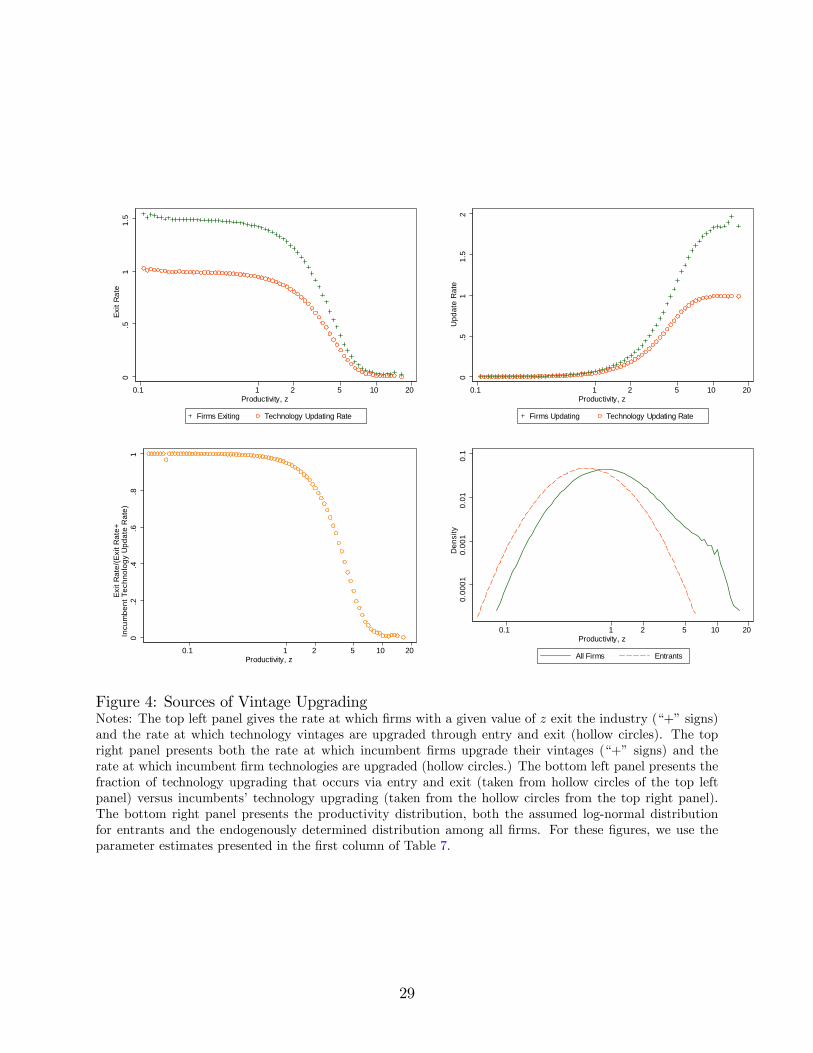
0.5

11.

5Ex

it R

ate

0.1 1 2 5 10 20Productivity, z

Firms Exiting Technology Updating Rate

0.5

11.

52

Upd

ate 

Rat

e

0.1 1 2 5 10 20Productivity, z

Firms Updating Technology Updating Rate

0.2

.4.6

.81

Exit 

Rat

e/(E

xit R

ate+

Incu

mbe

nt T

echn

olog

y U

pdat

e R

ate)

0.1 1 2 5 10 20Productivity, z

0.1

0.01

0.00

10.

0001

Den

sity

0.1 1 2 5 10 20Productivity, z

All Firms Entrants

Figure 4: Sources of Vintage UpgradingNotes: The top left panel gives the rate at which firms with a given value of z exit the industry (“+”signs)and the rate at which technology vintages are upgraded through entry and exit (hollow circles). The topright panel presents both the rate at which incumbent firms upgrade their vintages (“+” signs) and therate at which incumbent firm technologies are upgraded (hollow circles.) The bottom left panel presents thefraction of technology upgrading that occurs via entry and exit (taken from hollow circles of the top leftpanel) versus incumbents’technology upgrading (taken from the hollow circles from the top right panel).The bottom right panel presents the productivity distribution, both the assumed log-normal distributionfor entrants and the endogenously determined distribution among all firms. For these figures, we use theparameter estimates presented in the first column of Table 7.

29

for such workers ultimately perform poorly or disappear. In sum, since many employer-

employee relationships are long-lived, vacancy postings not only lead to new hires, but also

provide a window to researchers on firms’aspirations and capabilities over the next several

years.

Motivated by these patterns, we develop an industry equilibriummodel of technology

upgrading. As time progresses, firms fall further and further behind the technological fron-

tier, and, without successfully upgrading their technology, exit the industry. Exiting firms

are replaced by entrants with relatively newer vintage technologies. We estimate our model

using information on the distribution of firms’sales, ages, and job title vintages. Based on

this estimation, we find that both channels of technology upgrading play an important role.

Our starting point in this paper has been to construct a single summary measure

of firms’adoption of new technologies. But our approach, drawing on detailed information

from the job ads that firms place, permits richer analyses, differentiating jobs according to

their function. Certain groups of jobs are informative about firms’innovative activities in

managerial and organizational domains; other groups of jobs are informative about firms’

technological capabilities. Do firms’placement of newer vintage organizational and tech-

nological job ads occur at different points in their life cycles? Are hiring for newer work

practices in organizational jobs and technological jobs complementary to one another? We

leave an analysis of these questions to future work.

References

Aghion, P., U. Akcigit, and P. Howitt (2014): “What Do We Learn from Schum-

peterian Growth Theory?,”Handbook of Economic Growth, 2, 515—563.

Akcigit, U., andW. Kerr (2018): “Growth through Heterogeneous Innovations,”Journal

of Political Economy, 126(4), 1374—1443.

Anzoategui, D., D. Comin, M. Gertler, and J. Martinez (2019): “Endogenous Tech-

nology Adoption and R&D as Sources of Business Cycle Persistence,”American Economic

Journal: Macroeconomics, 11(3), 67—110.

Argente, D., S. Baslandze, D. Hanley, and S. Moreira (2020): “Patents to Prod-

ucts: Innovation, Product Creation, and Firm Growth,”Working Paper.

Atalay, E., P. Phongthiengtham, S. Sotelo, and D. Tannenbaum (2018): “New

Technologies and the Labor Market,”Journal of Monetary Economics, 97, 48—67.

30

(2020): “The Evolving U.S. Occupational Structure,”American Economic Journal:

Applied Economics, 12(2), 1—36.

Brown, J., and D. A. Matsa (2016): “Boarding a Sinking Ship? An Investigation of Job

Applications to Distressed Firms,”Journal of Finance, 71(2), 507—550.

Bulkeley, W. M. (1978): “American Biltrite Out of Intensive Care, Revived by Presi-

dent’sTight Controls,”Wall Street Journal, 27, 18.

Caselli, F. (1999): “Technological Revolutions,”American Economic Review, 89(1), 78—

102.

Ceruzzi, P. E. (2003): A History of Modern Computing. MIT Press.

Chari, V., and H. Hopenhayn (1991): “Vintage Human Capital, Growth, and the Diffu-

sion of New Technology,”Journal of Political Economy, 99(6), 1142—65.

Comin, D., and B. Hobijn (2004): “Cross-Country Technology Adoption: Making the

Theories Face the Facts,”Journal of Monetary Economics, 51(1), 39—83.

(2010): “An Exploration of Technology Diffusion,”American Economic Review,

100(5), 2031—2059.

Conley, T., and C. Udry (2010): “Learning about a New Technology: Pineapple in

Ghana,”American Economic Review, 100(1), 35—69.

Deming, D., and L. B. Kahn (2018): “Skill Requirements Across Firms and Labor Mar-

kets: Evidence from Job Postings for Professionals,”Journal of Labor Economics, 36(S1),

S337—S369.

Deming, D., and K. Noray (2019): “STEM Careers and the Changing Skill Content of

Work,”.

Garcia-Macia, D., C.-T. Hsieh, and P. Klenow (2019): “How Destructive Is Innova-

tion?,”Econometrica, 87(5), 1507—1541.

Gort, M., and S. Klepper (1982): “Time Paths in the Diffusion of Product Innovations,”

Economic Journal, 92(367), 630—653.

Greenwood, J., and M. Yorukoglu (1997): “1974,” Carnegie-Rochester Conference

Series on Public Policy, 46, 49—96.

31

Henderson, R. M., and K. B. Clark (1990): “Architectural Innovation: The Reconfig-

uration of Existing Product Technologies and the Failure of Established Firms,”Admin-

istrative Science Quarterly, 35(1), 9—30.

Jovanovic, B., and S. Lach (1989): “Entry, Exit, and Diffusion with Learning by Doing,”

American Economic Review, 79(4), 690—699.

Jovanovic, B., and G. MacDonald (1994): “The Life Cycle of a Competitive Industry,”

Journal of Political Economy, 102(2), 322—347.

Jovanovic, B., and Y. Yatsenko (2012): “Investment in Vintage Capital,” Journal of

Economic Theory, 147(2), 551—569.

Klette, T. J., and S. Kortum (2004): “Innovating Firms and Aggregate Innovation,”

Journal of Political Economy, 112(3), 986—1018.

Lin, J. (2011): “Technological Adaptation, Cities, and New Work,”Review of Economics

and Statistics, 93(2), 554—574.

Raffo, J. (2015): “MATCHIT: Stata Module to Match Two Datasets Based on Similar

Text Patterns,”Statistical Software Component.

Spitz-Oener, A. (2006): “Technical Change, Job Tasks, and Rising Educational Demands:

Looking Outside the Wage Structure,”Journal of Labor Economics, 24(2), 235—270.

A Additional Details on Processing the Job Ad Text

In this appendix, drawing on Atalay, Phongthiengtham, Sotelo, and Tannenbaum (2018,

2020), we outline the steps necessary to extract task and technology mentions from the job

ad text. Then, we describe the way in which we extract information about the entity posting

the ad, how we extract the posted salary, and how we compute the vintage of each job title.

Parts of the following paragraph quotes directly from (Atalay, Phongthiengtham, Sotelo, and

Tannenbaum, 2018, p. 50).

The original newspapers were digitized by ProQuest using an Optical Character

Recognition (OCR) technology. We briefly describe the steps we take to transform this

digitized text into a structured database. To begin, the raw text does not distinguish between

job ads and other types of advertisements. Hence, in a first step, we apply a machine

learning algorithm to determine which pages of advertisements are job ads. In a second

step we extract, from each advertisement, words that refer to tasks the new hire is expected

32

to perform and technologies that will be used on the job. So that we may link the text-

based data to occupation-level variables in the decennial census, including wages, education,

and demographic variables, the procedure also finds the Standard Occupation Classification

(SOC) code corresponding to each job title. In addition, we search for mentions of 48

individual technologies which are mentioned at various points of the 1940.26

New to this paper, we extract information on the entity which posted the vacancy

posting. To do so, we begin by searching within the job ad text for three types of strings:

First, we search for strings which indicate a firm name: “agency,”“agcy,”“associates,”“as-

soc,”“co,”“company,”“corp,”“corporation,”“inc,”“incorporated,”“llc,”and “personnel.”

Second, we search for a 7-digit number (which would indicate a phone number) that does

not begin with “0”or a “1”(in the United States phone numbers do not begin with these

digits) and does not have a “$” preceding it. Third, we search for strings that indicate

an address: “ave,”“st,”“42nd,”“bway,”“wall,”and “box.”Having extracted strings that

fit one these three forms, we next manually combine common firm names from the first

list of strings. For example, for any job title which contains the string “3m company”or

“minnesota mining manufacturing co,”we assign the posting firm to be the “3m company.”

Next, for each commonly appearing phone number, we examine whether (within the same

set of ads) there is a firm name which also uniquely appears. If so, for any ads for which

this phone number appears but the firm name does not, we then assign the firm name from

the set of ads for which the commonly appearing phone number appears with a firm name.

(For instance, suppose there is some phone number – e.g., 555-5555 – appearing in ads for

the 3m company. In any ads for which 555-5555 appears but the 3m company does not, we

re-assign the firm name to be the 3m company.) In instances in which commonly appearing

phone numbers do not map to firm names, we retain the phone number as the identifier of

the posting entity. In a final step, for ads for which a firm name is not yet assigned, we

then manually assign firm names based on addresses. For instance, “341 madison 44 st”

appears as an address for which we had previously identified the Taft Agency as the posting

firm. Thus, for ads for which we observe “341 madison 44 st”but not the posting firm, we

re-assign the posting firm to be the Taft Agency.

Finally, we extract information on the salary which the applicant would be paid. To

do so, we search for groups of strings indicating a salary. A main diffi culty to contend with is

that certain employers quote salaries on an annual basis, others on a weekly or hourly basis.

26These 48 technologies are APL, BAL, CAD, CICS, CNC, COBOL, C++, DB2, DOS, EDP, FORTRAN,FoxPro, HTML, IBM 360, IBM 370, IBM 5520, IBM RPG, Java, JCL, LAN, Lotus 123, Lotus Notes, MSExcel, MS PowerPoint, MS Word, MVS, Novell, Oracle, PASCAL, Point of Sale, PowerBuilder, Quark,Sabre, SQL, Sybase, TCP, TSO, UNIVAC, Unix, VAX, Visual Basic, VMS, VSAM, Vydec, WordPerfect,Xerox 630, Xerox 800, and Xerox 860.

33

With this in mind, we search for the following sets of strings to indicate an annual salary:

• “to x 000,”“$ x 000,”where x is a number between 5 and 39, between 40 and 100(searching in multiples of 5), and between 100 and 250 (searching in multiples of 25);

• “to x 500,”“$ x 500,”where x is a number between 5 and 14

• “ xk ,” where x is a number between 8 and 39, between 40 and 100 (searching inmultiples of 5), and between 100 and 250 (searching in multiples of 25).

Within these searches, we restrict attention to ads in which there is at most one dollar

sign (since multiple dollar signs may indicate multiple possible salaries.) Further, we search

for additional common strings, indicating other possible salaries:

• the string “$ 8 10 000,” for instance, would indicate a salary range of eight to tenthousand dollars. From this, we record a salary of “$10,000”

Additionally, we search for weekly salaries. To do so, we search for strings of the

form:

• “$ x y”where x is a number between 40 and 160 (in multiples of 5) and y is equal tox + 5 or x + 10. In instances like this, the firm is indicating a salary range of x to y

per week. For jobs like this, we record the number y to be the salary.

• “$ x wk,”“$ x per wk,”“$ x week,”or “$ x per week”for x between 20 and 300 (inmultiples of 5).

Also within these searches, we restrict attention to ads in which there is at most one

dollar sign. Further, we search for additional common strings, for example:

• the string “$ 35 50,”“ $ 55 70,”“$ 80 100”to indicate weekly salaries of $50, $70, or$100.

Finally, we search for hourly wages by searching for stings of the form “x yz hr,”“x yz

per hr,”or “x yz per hour”where x, y, and z are numbers.

34

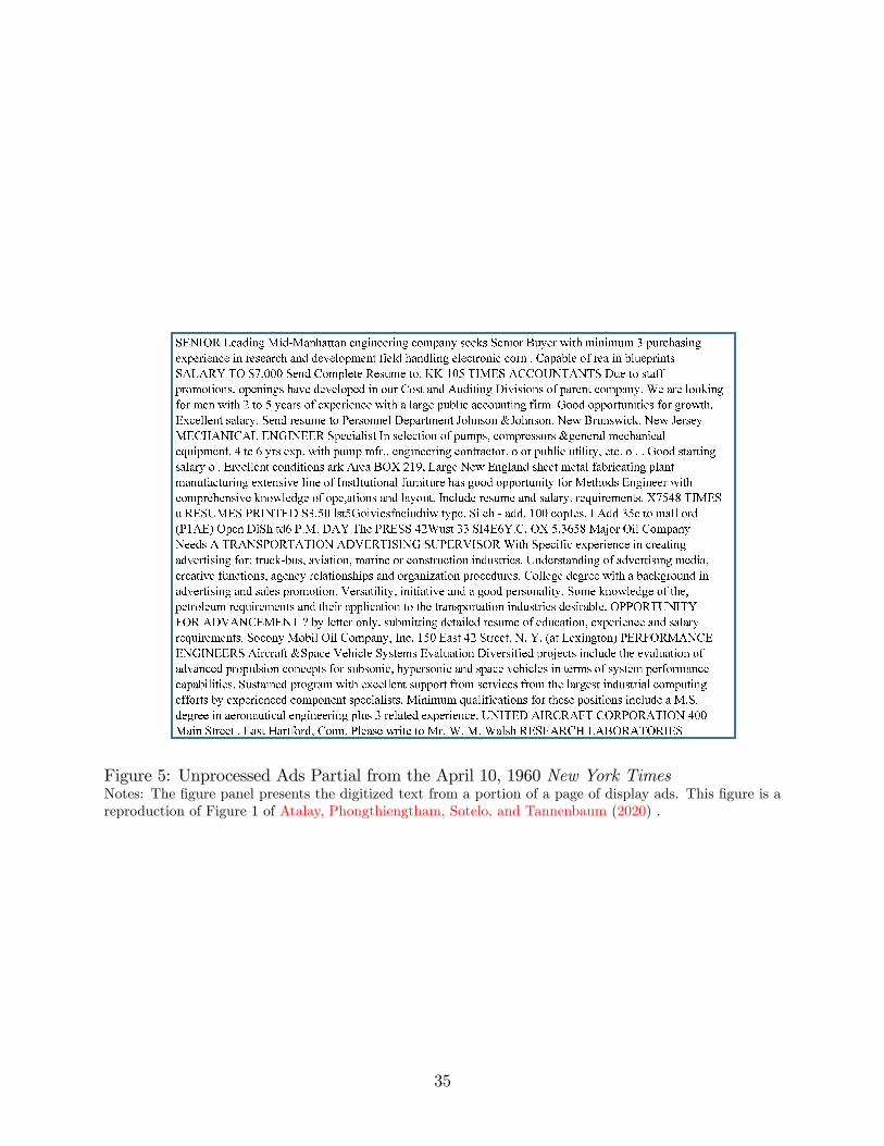
Figure 5: Unprocessed Ads Partial from the April 10, 1960 New York TimesNotes: The figure panel presents the digitized text from a portion of a page of display ads. This figure is areproduction of Figure 1 of Atalay, Phongthiengtham, Sotelo, and Tannenbaum (2020) .

35

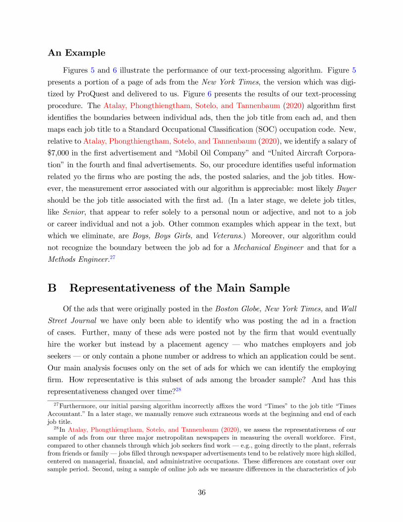
An Example

Figures 5 and 6 illustrate the performance of our text-processing algorithm. Figure 5

presents a portion of a page of ads from the New York Times, the version which was digi-

tized by ProQuest and delivered to us. Figure 6 presents the results of our text-processing

procedure. The Atalay, Phongthiengtham, Sotelo, and Tannenbaum (2020) algorithm first

identifies the boundaries between individual ads, then the job title from each ad, and then

maps each job title to a Standard Occupational Classification (SOC) occupation code. New,

relative to Atalay, Phongthiengtham, Sotelo, and Tannenbaum (2020), we identify a salary of

$7,000 in the first advertisement and “Mobil Oil Company”and “United Aircraft Corpora-

tion”in the fourth and final advertisements. So, our procedure identifies useful information

related yo the firms who are posting the ads, the posted salaries, and the job titles. How-

ever, the measurement error associated with our algorithm is appreciable: most likely Buyer

should be the job title associated with the first ad. (In a later stage, we delete job titles,

like Senior, that appear to refer solely to a personal noun or adjective, and not to a job

or career individual and not a job. Other common examples which appear in the text, but

which we eliminate, are Boys, Boys Girls, and Veterans.) Moreover, our algorithm could

not recognize the boundary between the job ad for a Mechanical Engineer and that for a

Methods Engineer.27

B Representativeness of the Main Sample

Of the ads that were originally posted in the Boston Globe, New York Times, andWall

Street Journal we have only been able to identify who was posting the ad in a fraction

of cases. Further, many of these ads were posted not by the firm that would eventually

hire the worker but instead by a placement agency – who matches employers and job

seekers – or only contain a phone number or address to which an application could be sent.

Our main analysis focuses only on the set of ads for which we can identify the employing

firm. How representative is this subset of ads among the broader sample? And has this

representativeness changed over time?28

27Furthermore, our initial parsing algorithm incorrectly affi xes the word “Times”to the job title “TimesAccountant.”In a later stage, we manually remove such extraneous words at the beginning and end of eachjob title.28In Atalay, Phongthiengtham, Sotelo, and Tannenbaum (2020), we assess the representativeness of our

sample of ads from our three major metropolitan newspapers in measuring the overall workforce. First,compared to other channels through which job seekers find work – e.g., going directly to the plant, referralsfrom friends or family – jobs filled through newspaper advertisements tend to be relatively more high skilled,centered on managerial, financial, and administrative occupations. These differences are constant over oursample period. Second, using a sample of online job ads we measure differences in the characteristics of job

36

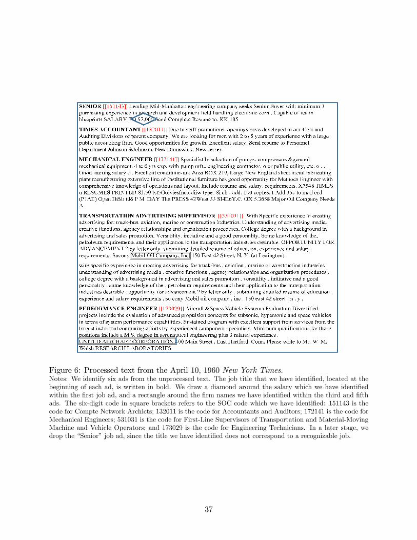
Figure 6: Processed text from the April 10, 1960 New York Times.Notes: We identify six ads from the unprocessed text. The job title that we have identified, located at thebeginning of each ad, is written in bold. We draw a diamond around the salary which we have identifiedwithin the first job ad, and a rectangle around the firm names we have identified within the third and fifthads. The six-digit code in square brackets refers to the SOC code which we have identified: 151143 is thecode for Compte Network Archicts; 132011 is the code for Accountants and Auditors; 172141 is the code forMechanical Engineers; 531031 is the code for First-Line Supervisors of Transportation and Material-MovingMachine and Vehicle Operators; and 173029 is the code for Engineering Technicians. In a later stage, wedrop the “Senior”job ad, since the title we have identified does not correspond to a recognizable job.

37

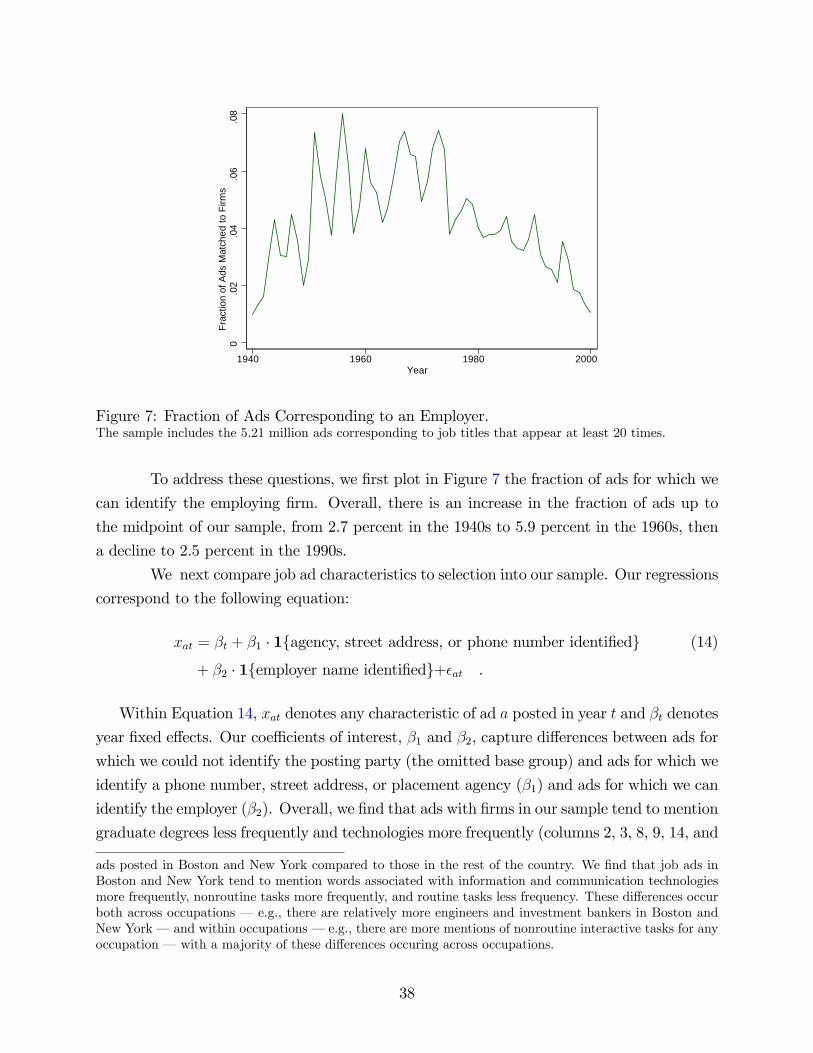
0.0

2.0

4.0

6.0

8Fr

actio

n of

 Ads

 Mat

ched

 to F

irms

1940 1960 1980 2000Year

Figure 7: Fraction of Ads Corresponding to an Employer.The sample includes the 5.21 million ads corresponding to job titles that appear at least 20 times.

To address these questions, we first plot in Figure 7 the fraction of ads for which we

can identify the employing firm. Overall, there is an increase in the fraction of ads up to

the midpoint of our sample, from 2.7 percent in the 1940s to 5.9 percent in the 1960s, then

a decline to 2.5 percent in the 1990s.

We next compare job ad characteristics to selection into our sample. Our regressions

correspond to the following equation:

xat = βt + β1 · 1{agency, street address, or phone number identified} (14)

+ β2 · 1{employer name identified}+εat .

Within Equation 14, xat denotes any characteristic of ad a posted in year t and βt denotes

year fixed effects. Our coeffi cients of interest, β1 and β2, capture differences between ads for

which we could not identify the posting party (the omitted base group) and ads for which we

identify a phone number, street address, or placement agency (β1) and ads for which we can

identify the employer (β2). Overall, we find that ads with firms in our sample tend to mention

graduate degrees less frequently and technologies more frequently (columns 2, 3, 8, 9, 14, and

ads posted in Boston and New York compared to those in the rest of the country. We find that job ads inBoston and New York tend to mention words associated with information and communication technologiesmore frequently, nonroutine tasks more frequently, and routine tasks less frequency. These differences occurboth across occupations – e.g., there are relatively more engineers and investment bankers in Boston andNew York – and within occupations – e.g., there are more mentions of nonroutine interactive tasks for anyoccupation – with a majority of these differences occuring across occupations.

38

15 of Table 8) To help gauge the economic significance of these estimates, in the final row of

each panel, we list within-year standard deviation of xft: the root mean squared error of a

regression of the job characteristic on year fixed effects. Ads with an employer observed have

0.09 standard deviations (≈ −0.670/7.551) fewer mentions of a graduate degree. Depending

on the job title vintage measure, ads in our benchmark sample have somewhat newer (in

the case of v0.01j(a)) or older (in the case of v0.99j(a)) job titles. In panels B and C, we compare

the estimated relationships across the two halves of our sample. We find that ads with an

identified posting firm tended have older job titles (using the v0.50j(a) measure) in the first half

of the sample but newer job titles in the second half. We also find that ads with a posting

firm tend to mention undergraduate degrees somewhat less frequently in the first half of the

sample, somewhat more frequently in the second half. Besides these two differences, there

were no notable differences in the estimate of β2 across the two halves of the sample.

C Additional Calculations Related to Section 3 and 4

C.1 Top Job Titles by Vintage

In this appendix, we presents a sample of the jobs which appeared and disappeared

within each decade of our sample period. The first panel lists the job titles which disappeared

by the end of the 1940s. According to the panel, the Lens Grinder, Radio Instructor,

Christmas Card Salesperson, and Fluorescent Salesperson are mentioned primarily in the

first decade of the sample. In later decades, job titles with the word “stenography” or

“stenographer”tend to disappear in the 1960s and 1970s; job titles with the word “keypunch”

or “typist”tend to disappear in the 1970s and 1980s. Conversely, job titles including “word

processing”or “word processor”tend to appear in the 1970s; “telemarketing”in the 1980s;

and “web”-related job titles in the 1990s.

C.2 Sensitivity Analysis Related to Section 4

Within Section 4 regressions our analysis weighted each observation according to the

number of ads corresponding to each firm-year observation. In this appendix, we present the

analogues of Tables 2- 6, with observations now weighted equally. Overall, we find that the

main patterns presented in Section 4 are invariant, qualitatively, to weighting observations

by the number of ads or not, though some of the magnitudes are smaller in unweighted

specifications.

39

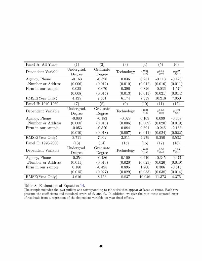
Panel A: All Years (1) (2) (3) (4) (5) (6)

Dependent VariableUndergrad.Degree

GraduateDegree

Technology v0.01j(a) v0.50j(a) v0.99j(a)

Agency, Phone -0.163 -0.328 0.036 0.251 -0.113 -0.423.Number or Address (0.006) (0.012) (0.010) (0.012) (0.016) (0.011)Firm in our sample 0.035 -0.670 0.396 0.826 -0.036 -1.570

(0.008) (0.015) (0.013) (0.015) (0.021) (0.014)RMSE(Year Only) 4.125 7.551 6.174 7.339 10.218 7.050Panel B: 1940-1969 (7) (8) (9) (10) (11) (12)

Dependent VariableUndergrad.Degree

GraduateDegree

Technology v0.01j(a) v0.50j(a) v0.99j(a)

Agency, Phone -0.080 -0.183 -0.028 0.109 0.099 -0.368.Number or Address (0.008) (0.015) (0.006) (0.009) (0.020) (0.019)Firm in our sample -0.053 -0.820 0.084 0.591 -0.245 -2.163

(0.010) (0.018) (0.007) (0.011) (0.024) (0.022)RMSE(Year Only) 3.711 7.062 2.811 4.279 9.250 8.532Panel C: 1970-2000 (13) (14) (15) (16) (17) (18)

Dependent VariableUndergrad.Degree

GraduateDegree

Technology v0.01j(a) v0.50j(a) v0.99j(a)

Agency, Phone -0.254 -0.486 0.109 0.410 -0.345 -0.477.Number or Address (0.011) (0.019) (0.020) (0.023) (0.026) (0.010)Firm in our sample 0.180 -0.425 0.895 1.200 0.306 -0.615

(0.015) (0.027) (0.029) (0.033) (0.038) (0.014)RMSE(Year Only) 4.616 8.153 8.837 10.046 11.373 4.375

Table 8: Estimation of Equation 14.The sample includes the 5.21 million ads corresponding to job titles that appear at least 20 times. Each rowpresents the coeffi cients and standard errors of β1 and β2. In addition, we give the root mean squared errorof residuals from a regression of the dependent variable on year fixed effects.

40

Disappearing Job Titles Emerging Job Titlesv0.99j ∈1940-49 v0.01j ∈1950-19591 lens grinder 1 administrative assistant2 radio instructor 2 programmer3 christmas card salesperson 3 legal secretary4 fluorescent salesperson 4 management trainee5 national tech 5 systems analystv0.99j ∈1950-1959 v0.01j ∈1960-19691 soda dispenser 1 programmer analyst2 millinery designer 2 computer operator3 buyer wants contd 3 marketing manager4 long distance telephone operator 4 product manager5 testy sales 5 medical centerv0.99j ∈1960-1969 v0.01j ∈1970-19791 house worker 1 paralegal2 bookkeeper stenographer 2 typesetter3 dental mechanic 3 word processing4 alteration hand 4 word processor5 collector salesperson 5 stock broker traineev0.99j ∈1970-1979 v0.01j ∈1980-19891 stenographer 1 telemarketer2 stenographer typist 2 hiv aid3 secretary stenographer 3 line cook4 offi ce boy 4 broker trainee5 comptometer operator 5 medical billerv0.99j ∈1980-1989 v0.01j ∈1990-20001 clerk typist 1 power builder2 draftsman 2 client server3 statistical typist 3 web developer4 biller typist 4 web master5 keypunch operator 5 actor auditions

Table 9: Top receding and emerging job titles.Notes: Each panel contains job titles which have v0.99j or v0.01j in a given decade. Within each panel, we listthe top five job titles, measured according to the number of ads in which the job title appears within the1940 to 2000 sample.

41

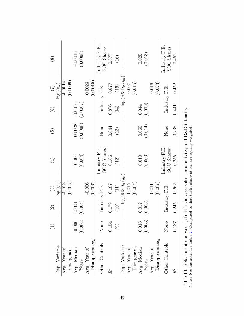
(1)

(2)

(3)

(4)

(5)

(6)

(7)

(8)

Dep.Variable

–––

log

(yit)

–––

––

log

(lp it)

––

Avg.Yearof

-0.013

-0.0014

Emergence it

(0.005)

(0.0009)

Avg.Median

-0.006

-0.004

-0.006

-0.0028

-0.0016

—0.0015

Year it

(0.004)(0.004)

(0.004)

(0.0008)

(0.0007)

(0.0008)

Avg.Yearof

-0.006

0.0023

Disappearanceit

(0.007)

(0.0015)

OtherControls

None

IndustryF.E.

IndustryF.E.

SOCShares

None

IndustryF.E.

IndustryF.E.

SOCShares

R2

0.154

0.179

0.187

0.186

0.844

0.876

0.877

0.877

(9)

(10)

(11)

(12)

(13)

(14)

(15)

(16)

Dep.Variable

––

log

(R&Dit/y

it)

––

––

log

(R&Dit/y

it)

––

Avg.Yearof

0.015

0.007

Emergence it

(0.004)

(0.015)

Avg.Median

0.013

0.012

0.010

0.060

0.044

0.025

Year it

(0.003)(0.003)

(0.003)

(0.014)

(0.012)

(0.013)

Avg.Yearof

0.011

0.016

Disappearanceit

(0.007)

(0.023)

OtherControls

None

IndustryF.E.

IndustryF.E.

SOCShares

None

IndustryF.E.

IndustryF.E.

SOCShares

R2

0.137

0.245

0.262

0.255

0.238

0.441

0.452

0.452

Table10:Relationshipbetweenjobtitlevintage,sales,productivity,andR&Dintensity.

Notes:SeethenotesforTable2.Comparedtothattable,observationsareequallyweighted.

42

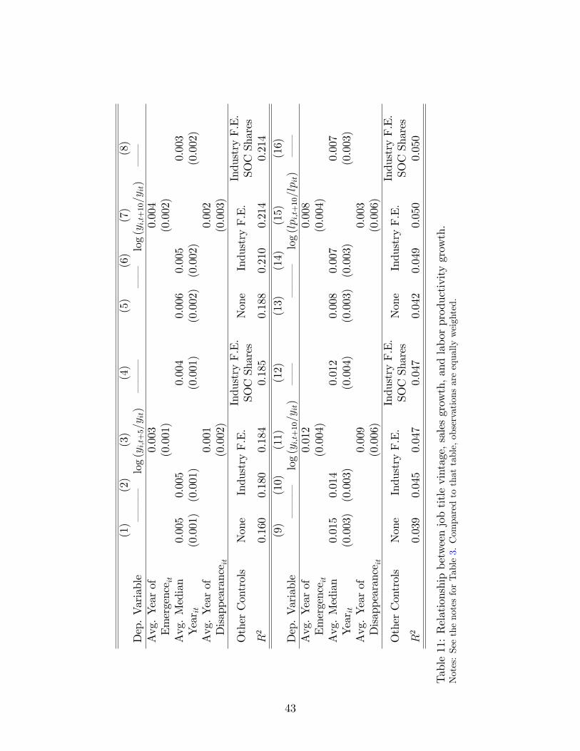
(1)

(2)

(3)

(4)

(5)

(6)

(7)

(8)

Dep.Variable

–––

log

(yi,t+5/y

it)

–––

––

log

(yi,t+10/y

it)

––

Avg.Yearof

0.003

0.004

Emergence it

(0.001)

(0.002)

Avg.Median

0.005

0.005

0.004

0.006

0.005

0.003

Year it

(0.001)(0.001)

(0.001)

(0.002)(0.002)

(0.002)

Avg.Yearof

0.001

0.002

Disappearanceit

(0.002)

(0.003)

OtherControls

None

IndustryF.E.

IndustryF.E.

SOCShares

None

IndustryF.E.

IndustryF.E.

SOCShares

R2

0.160

0.180

0.184

0.185

0.188

0.210

0.214

0.214

(9)

(10)

(11)

(12)

(13)

(14)

(15)

(16)

Dep.Variable

–––

log

(yi,t+10/y

it)

––

–––

log

(lp i,t+10/lp it)

––

Avg.Yearof

0.012

0.008

Emergence it

(0.004)

(0.004)

Avg.Median

0.015

0.014

0.012

0.008

0.007

0.007

Year it

(0.003)(0.003)

(0.004)

(0.003)(0.003)

(0.003)

Avg.Yearof

0.009

0.003

Disappearanceit

(0.006)

(0.006)

OtherControls

None

IndustryF.E.

IndustryF.E.

SOCShares

None

IndustryF.E.

IndustryF.E.

SOCShares

R2

0.039

0.045

0.047

0.047

0.042

0.049

0.050

0.050

Table11:Relationshipbetweenjobtitlevintage,salesgrowth,andlaborproductivitygrowth.

Notes:SeethenotesforTable3.Comparedtothattable,observationsareequallyweighted.

43

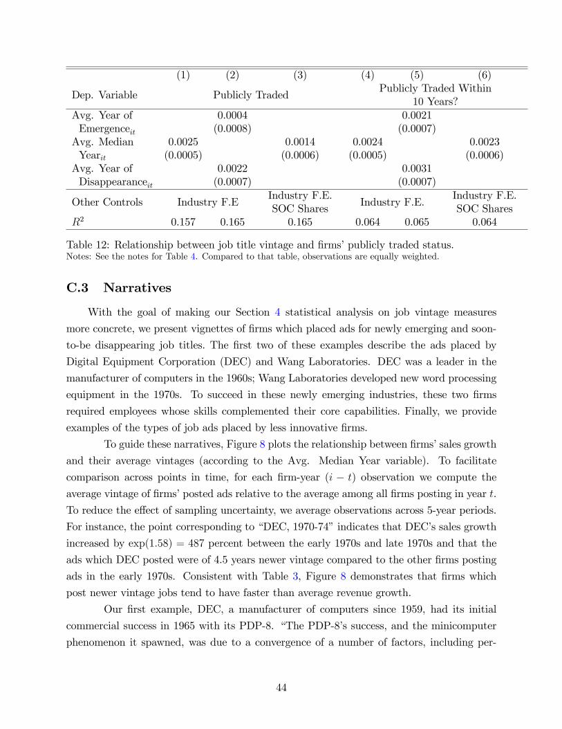
(1) (2) (3) (4) (5) (6)

Dep. Variable Publicly TradedPublicly Traded Within

10 Years?Avg. Year of 0.0004 0.0021Emergenceit (0.0008) (0.0007)Avg. Median 0.0025 0.0014 0.0024 0.0023Yearit (0.0005) (0.0006) (0.0005) (0.0006)Avg. Year of 0.0022 0.0031Disappearanceit (0.0007) (0.0007)

Other Controls Industry F.EIndustry F.E.SOC Shares

Industry F.E.Industry F.E.SOC Shares

R2 0.157 0.165 0.165 0.064 0.065 0.064

Table 12: Relationship between job title vintage and firms’publicly traded status.Notes: See the notes for Table 4. Compared to that table, observations are equally weighted.

C.3 Narratives

With the goal of making our Section 4 statistical analysis on job vintage measures

more concrete, we present vignettes of firms which placed ads for newly emerging and soon-

to-be disappearing job titles. The first two of these examples describe the ads placed by

Digital Equipment Corporation (DEC) and Wang Laboratories. DEC was a leader in the

manufacturer of computers in the 1960s; Wang Laboratories developed new word processing

equipment in the 1970s. To succeed in these newly emerging industries, these two firms

required employees whose skills complemented their core capabilities. Finally, we provide

examples of the types of job ads placed by less innovative firms.

To guide these narratives, Figure 8 plots the relationship between firms’sales growth

and their average vintages (according to the Avg. Median Year variable). To facilitate

comparison across points in time, for each firm-year (i − t) observation we compute the

average vintage of firms’posted ads relative to the average among all firms posting in year t.

To reduce the effect of sampling uncertainty, we average observations across 5-year periods.

For instance, the point corresponding to “DEC, 1970-74”indicates that DEC’s sales growth

increased by exp(1.58) = 487 percent between the early 1970s and late 1970s and that the

ads which DEC posted were of 4.5 years newer vintage compared to the other firms posting

ads in the early 1970s. Consistent with Table 3, Figure 8 demonstrates that firms which

post newer vintage jobs tend to have faster than average revenue growth.

Our first example, DEC, a manufacturer of computers since 1959, had its initial

commercial success in 1965 with its PDP-8. “The PDP-8’s success, and the minicomputer

phenomenon it spawned, was due to a convergence of a number of factors, including per-

44

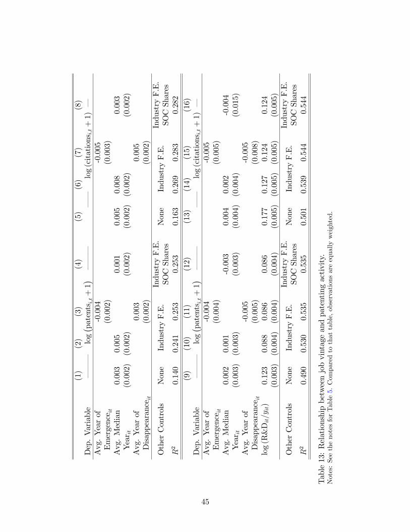
(1)

(2)

(3)

(4)

(5)

(6)

(7)

(8)

Dep.Variable

–––

log( pat

entsi,t+

1)–––

––

log

(citations

i,t+

1)–

Avg.Yearof

-0.004

-0.005

Emergence it

(0.002)

(0.003)

Avg.Median

0.003

0.005

0.001

0.005

0.008

0.003

Year it

(0.002)(0.002)

(0.002)

(0.002)(0.002)

(0.002)

Avg.Yearof

0.003

0.005

Disappearanceit

(0.002)

(0.002)

OtherControls

None

IndustryF.E.

IndustryF.E.

SOCShares

None

IndustryF.E.

IndustryF.E.

SOCShares

R2

0.140

0.241

0.253

0.253

0.163

0.269

0.283

0.282

(9)

(10)

(11)

(12)

(13)

(14)

(15)

(16)

Dep.Variable

–––

log( pat

entsi,t+

1)–––

––

log

(citations

i,t+

1)–

Avg.Yearof

-0.004

-0.005

Emergence it

(0.004)

(0.005)

Avg.Median

0.002

0.001

-0.003

0.004

0.002

-0.004

Year it

(0.003)(0.003)

(0.003)

(0.004)(0.004)

(0.015)

Avg.Yearof

-0.005

-0.005

Disappearanceit

(0.005)

(0.008)

log

(R&Dit/y

it)

0.123

0.088

0.086

0.086

0.177

0.127

0.124

0.124

(0.003)(0.004)(0.004)

(0.004)

(0.005)(0.005)(0.005)

(0.005)

OtherControls

None

IndustryF.E.

IndustryF.E.

SOCShares

None

IndustryF.E.

IndustryF.E.

SOCShares

R2

0.490

0.530

0.535

0.535

0.501

0.539

0.544

0.544

Table13:Relationshipbetweenjobvintageandpatentingactivity.

Notes:SeethenotesforTable5.Comparedtothattable,observationsareequallyweighted.

45

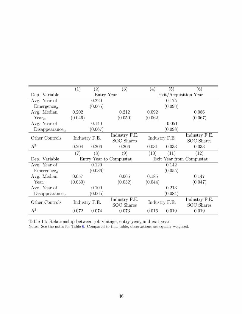
(1) (2) (3) (4) (5) (6)Dep. Variable Entry Year Exit/Acquisition YearAvg. Year of 0.220 0.175Emergenceit (0.065) (0.093)Avg. Median 0.202 0.212 0.092 0.086Yearit (0.046) (0.050) (0.062) (0.067)Avg. Year of 0.140 -0.051Disappearanceit (0.067) (0.098)

Other Controls Industry F.E.Industry F.E.SOC Shares

Industry F.E.Industry F.E.SOC Shares

R2 0.204 0.206 0.206 0.031 0.033 0.033(7) (8) (9) (10) (11) (12)

Dep. Variable Entry Year to Compustat Exit Year from CompustatAvg. Year of 0.120 0.142Emergenceit (0.036) (0.055)Avg. Median 0.057 0.065 0.185 0.147Yearit (0.030) (0.032) (0.044) (0.047)Avg. Year of 0.100 0.213Disappearanceit (0.065) (0.084)

Other Controls Industry F.E.Industry F.E.SOC Shares

Industry F.E.Industry F.E.SOC Shares

R2 0.072 0.074 0.073 0.016 0.019 0.019

Table 14: Relationship between job vintage, entry year, and exit year.Notes: See the notes for Table 6. Compared to that table, observations are equally weighted.

46

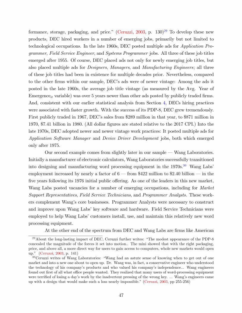
formance, storage, packaging, and price.” (Ceruzzi, 2003, p. 130)29 To develop these new

products, DEC hired workers in a number of emerging jobs, primarily but not limited to

technological occupations. In the late 1960s, DEC posted multiple ads for Application Pro-

grammer, Field Service Engineer, and Systems Programmer jobs. All three of these job titles

emerged after 1955. Of course, DEC placed ads not only for newly emerging job titles, but

also placed multiple ads for Designers, Managers, and Manufacturing Engineers; all three

of these job titles had been in existence for multiple decades prior. Nevertheless, compared

to the other firms within our sample, DEC’s ads were of newer vintage: Among the ads it

posted in the late 1960s, the average job title vintage (as measured by the Avg. Year of

Emergenceit variable) was over 5 years newer than other ads posted by publicly traded firms.

And, consistent with our earlier statistical analysis from Section 4, DECs hiring practices

were associated with faster growth. With the success of its PDP-8, DEC grew tremendously.

First publicly traded in 1967, DEC’s sales from $289 million in that year, to $871 million in

1970, $7.41 billion in 1980. (All dollar figures are stated relative to the 2017 CPI.) Into the

late 1970s, DEC adopted newer and newer vintage work practices: It posted multiple ads for

Application Software Manager and Device Driver Development jobs, both which emerged

only after 1975.

Our second example comes from slightly later in our sample – Wang Laboratories.

Initially a manufacturer of electronic calculators, Wang Laboratories successfully transitioned

into designing and manufacturing word processing equipment in the 1970s.30 Wang Labs’

employment increased by nearly a factor of 6 – from $422 million to $2.40 billion – in the

five years following its 1976 initial public offering. As one of the leaders in this new market,

Wang Labs posted vacancies for a number of emerging occupations, including for Market

Support Representatives, Field Service Technicians, and Programmer Analysts. These work-

ers complement Wang’s core businesses. Programmer Analysts were necessary to construct

and improve upon Wang Labs’key software and hardware. Field Service Technicians were

employed to help Wang Labs’customers install, use, and maintain this relatively new word

processing equipment.

At the other end of the spectrum from DEC and Wang Labs are firms like American

29About the long-lasting impact of DEC, Ceruzzi further writes: “The modest appearance of the PDP-8concealed the magnitude of the forces it set into motion.. The mini showed that with the right packaging,price, and above all, a more direct way for users to gain access to computers, whole new markets would openup.” (Ceruzzi, 2003, p. 141)30Ceruzzi writes of Wang Laboratories: “Wang had an astute sense of knowing when to get out of one

market and into a new one about to open up. Dr. Wang was, in fact, a conservative engineer who understoodthe technology of his company’s products and who valued his company’s independence... Wang engineersfound out first of all what offi ce people wanted. They realized that many users of word-processing equipmentwere terrified of losing a day’s work by the inadvertent pressing of the wrong key. ... Wang’s engineers cameup with a design that would make such a loss nearly impossible.”(Ceruzzi, 2003, pp 255-256)

47

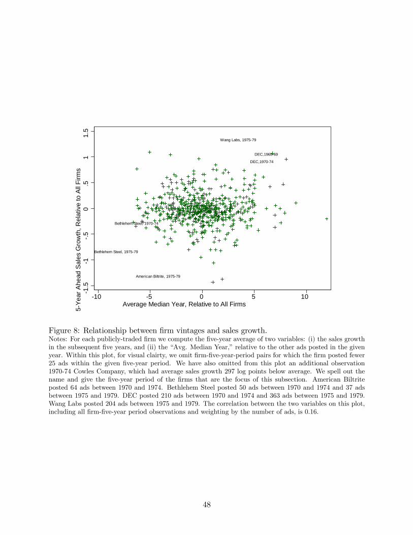
Wang Labs, 1975­79

DEC,1965­69

DEC,1970­74

American Biltrite, 1975­79

Bethlehem Steel, 1975­79

Bethlehem Steel, 1970­74

­1.5

­1­.5

0.5

11.

55­

Year

 Ahe

ad S

ales

 Gro

wth

, Rel

ativ

e to

 All 

Firm

s

­10 ­5 0 5 10Average Median Year, Relative to All Firms

Figure 8: Relationship between firm vintages and sales growth.Notes: For each publicly-traded firm we compute the five-year average of two variables: (i) the sales growthin the subsequent five years, and (ii) the “Avg. Median Year,”relative to the other ads posted in the givenyear. Within this plot, for visual clairty, we omit firm-five-year-period pairs for which the firm posted fewer25 ads within the given five-year period. We have also omitted from this plot an additional observation1970-74 Cowles Company, which had average sales growth 297 log points below average. We spell out thename and give the five-year period of the firms that are the focus of this subsection. American Biltriteposted 64 ads between 1970 and 1974. Bethlehem Steel posted 50 ads between 1970 and 1974 and 37 adsbetween 1975 and 1979. DEC posted 210 ads between 1970 and 1974 and 363 ads between 1975 and 1979.Wang Labs posted 204 ads between 1975 and 1979. The correlation between the two variables on this plot,including all firm-five-year period observations and weighting by the number of ads, is 0.16.

48

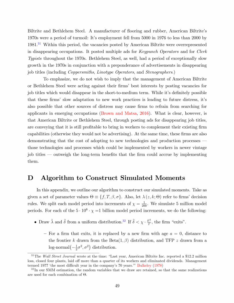
Biltrite and Bethlehem Steel. A manufacturer of flooring and rubber, American Biltrite’s

1970s were a period of turmoil: It’s employment fell from 5000 in 1976 to less than 2000 by

1981.31 Within this period, the vacancies posted by American Biltrite were overrepresented

in disappearing occupations. It posted multiple ads for Keypunch Operators and for Clerk

Typists throughout the 1970s. Bethlehem Steel, as well, had a period of exceptionally slow

growth in the 1970s in conjunction with a preponderance of advertisements in disappearing

job titles (including Coppersmiths, Linotype Operators, and Stenographers.)

To emphasize, we do not wish to imply that the management of American Biltrite

or Bethlehem Steel were acting against their firms’best interests by posting vacancies for

job titles which would disappear in the short-to-medium term. While it’s definitely possible

that these firms’ slow adaptation to new work practices is leading to future distress, it’s

also possible that other sources of distress may cause firms to refrain from searching for

applicants in emerging occupations (Brown and Matsa, 2016). What is clear, however, is

that American Biltrite or Bethlehem Steel, through posting ads for disappearing job titles,

are conveying that it is still profitable to bring in workers to complement their existing firm

capabilities (otherwise they would not be advertising). At the same time, these firms are also

demonstrating that the cost of adopting to new technologies and production processes –

those technologies and processes which could be implemented by workers in newer vintage

job titles – outweigh the long-term benefits that the firm could accrue by implementing

them.

D Algorithm to Construct Simulated Moments

In this appendix, we outline our algorithm to construct our simulated moments. Take as

given a set of parameter values Θ ≡ {f, T, β, σ}. Also, let λ (z, k; Θ) refer to firms’decision

rules. We split each model period into increments of χ = 1200. We simulate 5 million model

periods. For each of the 5 · 106 · χ =1 billion model period increments, we do the following:

• Draw λ̃ and δ̃ from a uniform distribution.32 If δ̃ < χ · δAT, the firm “exits”.

—For a firm that exits, it is replaced by a new firm with age a = 0, distance to

the frontier k drawn from the Beta(1, β) distribution, and TFP z drawn from a

log-normal(−12σ2, σ2

)distribution.

31The Wall Street Journal wrote at the time: “Last year, American Biltrite Inc. reported a $12.2 millionloss, closed four plants, laid off more than a quarter of its workers and eliminated dividends. Managementtermed 1977 ‘the most diffi cult year in the company’s 70 years.’”Bulkeley (1978)32In our SMM estimation, the random variables that we draw are retained, so that the same realizations

are used for each combination of Θ.

49

• If δ̃ > χ · δATand λ̃ < λ (z, k; Θ) · χ, the firm updates its vintage:

—For a firm that updates its vintage, the age a increases by χ, and the distance to

the frontier k equals 0.

• If δ̃ > χ · δATand λ̃ > λ (z, k; Θ) · χ:

— If k < 1, the age and distance to the frontier each increase by χ.

— If k = 1, the firm exits. It is replaced by a new firm with age a = 0, distance to

the frontier k drawn from the Beta(1, β) distribution, and TFP z drawn from a

log-normal(−12σ2, σ2

)distribution.

The result of this procedure is a sample of 1 billion observations, with each observa-

tion containing information on age (a), TFP (z), and distance to the frontier (k). Note that

log sales is proportional to log TFP.

50