Emergent relationships on burned area in global satellite

Emergent relationships on burned area in global satellite observations and fire-enabled vegetation models Article

Published Version

Creative Commons: Attribution 4.0 (CC-BY)

Open Access

Forkel, M., Andela, N., Harrison, S. P., Lasslop, G., van Marle, M., Chuvieco, E., Dorigo, W., Forrest, M., Hantson, S., Heil, A., Li, F., Melton, J., Sitch, S., Yue, C. and Arneth, A. (2019) Emergent relationships on burned area in global satellite observations and fire-enabled vegetation models. Biogeosciences, 16. pp. 57-76. ISSN 1726-4170 doi: https://doi.org/10.5194/bg-16-57-2019 Available at https://centaur.reading.ac.uk/81127/

It is advisable to refer to the publisher’s version if you intend to cite from the work. See Guidance on citing .

To link to this article DOI: http://dx.doi.org/10.5194/bg-16-57-2019

Publisher: Copernicus Publications

All outputs in CentAUR are protected by Intellectual Property Rights law, including copyright law. Copyright and IPR is retained by the creators or other copyright holders. Terms and conditions for use of this material are defined in the End User Agreement .

www.reading.ac.uk/centaur

http://centaur.reading.ac.uk/71187/10/CentAUR%20citing%20guide.pdf

http://www.reading.ac.uk/centaur

http://centaur.reading.ac.uk/licence

CentAUR

Central Archive at the University of Reading Reading’s research outputs online

Biogeosciences, 16, 57–76, 2019https://doi.org/10.5194/bg-16-57-2019© Author(s) 2019. This work is distributed underthe Creative Commons Attribution 4.0 License.

Emergent relationships with respect to burned area in globalsatellite observations and fire-enabled vegetation modelsMatthias Forkel1, Niels Andela2, Sandy P. Harrison3, Gitta Lasslop4, Margreet van Marle5, Emilio Chuvieco6,Wouter Dorigo1, Matthew Forrest4, Stijn Hantson7, Angelika Heil8, Fang Li9, Joe Melton10, Stephen Sitch11,Chao Yue12, and Almut Arneth13

1Climate and Environmental Remote Sensing Group, Department of Geodesy and Geoinformation,Technische Universität Wien, Vienna, Austria2Biospheric Sciences Laboratory, NASA Goddard Space Flight Center, Greenbelt, MD, USA3Department of Geography and Environmental Science, University of Reading, Reading, UK4Senckenberg Biodiversity and Climate Research Centre, Frankfurt am Main, Germany5Deltares, Delft, the Netherlands6Environmental Remote Sensing Research Group, Department of Geology, Geography and the Environment,Universidad de Alcalá, Alcalá de Henares, Spain7Geospatial Data Solutions Center, University of California, Irvine, CA, USA8Department for Atmospheric Chemistry, Max Planck Institute for Chemistry, Mainz, Germany9International Center for Climate and Environmental Sciences, Institute of Atmospheric Physics,Chinese Academy of Sciences, Beijing, China10Climate Research Division, Environment Canada, Victoria, BC, Canada11College of Life and Environmental Sciences, University of Exeter, Exeter, UK12Laboratoire des Sciences du Climat et de l’Environnement, Gif-sur-Yvette, France13Atmospheric Environmental Research, Institute of Meteorology and Climate Research,Karlsruhe Institute of Technology, Garmisch-Partenkirchen, Germany

Correspondence: Matthias Forkel ([email protected])

Received: 28 September 2018 – Discussion started: 18 October 2018Revised: 5 December 2018 – Accepted: 11 December 2018 – Published: 11 January 2019

Abstract. Recent climate changes have increased fire-proneweather conditions in many regions and have likely affectedfire occurrence, which might impact ecosystem function-ing, biogeochemical cycles, and society. Prediction of howfire impacts may change in the future is difficult becauseof the complexity of the controls on fire occurrence andburned area. Here we aim to assess how process-based fire-enabled dynamic global vegetation models (DGVMs) rep-resent relationships between controlling factors and burnedarea. We developed a pattern-oriented model evaluation ap-proach using the random forest (RF) algorithm to iden-tify emergent relationships between climate, vegetation, andsocio-economic predictor variables and burned area. We ap-plied this approach to monthly burned area time series forthe period from 2005 to 2011 from satellite observations

and from DGVMs from the “Fire Modeling Intercompari-son Project” (FireMIP) that were run using a common proto-col and forcing data sets. The satellite-derived relationshipsindicate strong sensitivity to climate variables (e.g. maxi-mum temperature, number of wet days), vegetation proper-ties (e.g. vegetation type, previous-season plant productivityand leaf area, woody litter), and to socio-economic variables(e.g. human population density). DGVMs broadly reproducethe relationships with climate variables and, for some mod-els, with population density. Interestingly, satellite-derivedresponses show a strong increase in burned area with an in-crease in previous-season leaf area index and plant produc-tivity in most fire-prone ecosystems, which was largely un-derestimated by most DGVMs. Hence, our pattern-orientedmodel evaluation approach allowed us to diagnose that veg-

Published by Copernicus Publications on behalf of the European Geosciences Union.

58 M. Forkel et al.: Emergent relationships with respect to burned area

etation effects on fire are a main deficiency regarding fire-enabled dynamic global vegetation models’ ability to accu-rately simulate the role of fire under global environmentalchange.

1 Introduction

About 3 % of the global land area burns every year (Chu-vieco et al., 2016; Giglio et al., 2013; Randerson et al.,2012). Fire represents a strong control on large-scale veg-etation patterns and structure (Bond et al., 2004) and cansignificantly accelerate the impacts of changing climate orland management on global ecosystems (Aragão et al., 2018;Beck et al., 2011). Fire directly affects global and regionalclimate through changing surface albedo (López-Saldaña etal., 2015; Randerson et al., 2006), atmospheric trace gas, andaerosol concentrations (Andreae and Merlet, 2001; Ward etal., 2012), and on longer timescales by affecting vegetationcomposition and structure with subsequent impacts on thecarbon cycle and hydrology (Li and Lawrence, 2016; Pausasand Dantas, 2017; Tepley et al., 2018; Thonicke et al., 2001).

Climate influences several aspects of the fire regime, in-cluding the seasonal timing of lightning ignitions (Veraver-beke et al., 2017), temperature and moisture controls onfuel drying, and wind-driven fire spread (Jolly et al., 2015).Climate also influences the nature and availability of fuel,through its impact on vegetation productivity and structure(Harrison et al., 2010). Vegetation structure, in turn, influ-ences the patterns of available fuel and moisture that directlydetermine fire spread, severity, and extent (Krawchuk andMoritz, 2011; Pausas and Ribeiro, 2013). People set and sup-press fires and use them to manage agricultural and naturalecosystems, for land use change and deforestation practices(Andela and van der Werf, 2014; van Marle et al., 2017).Human-induced modifications and fragmentation of naturalvegetation through agricultural expansion and urbanizationlimit fire spread (Bowman et al., 2011). Thus, climate, vege-tation, and human controls on fire are multivariate and havestrong interactions with one another (Bowman et al., 2009;Harrison et al., 2010; Krawchuk et al., 2009). Empirical anal-yses of fire regimes using machine learning algorithms haveidentified the most important variables and their sensitivi-ties for fire occurrence and spread (Aldersley et al., 2011;Archibald et al., 2009; Bistinas et al., 2014; Forkel et al.,2017; Krawchuk et al., 2009; Moritz et al., 2012). How-ever, because of the difficulty of factoring out interactions be-tween predictor variables, such sensitivities represent emer-gent relationships rather than specific physical controls onfire. Thus, it has proved difficult to disentangle the role ofchanges in any single factor on the trajectory of changesin fire regimes. For example, changes in climate result inweather conditions that are increasingly favourable for fireand fire activity in some temperate regions (Holden et al.,

2018; Jolly et al., 2015; Müller et al., 2015); however, it hasbeen suggested that changes in land use compensate for cli-mate effects and result, for example, in declining burned ar-eas in African savannahs (Andela and van der Werf, 2014).Hence, there is still uncertainty regarding factors such asthe cause of the recent observed decline in global burnedarea (Andela et al., 2017). Furthermore, there is even greateruncertainty about the potential trajectory of changes in fireregimes in the future (Settele et al., 2014).

Fire-enabled dynamic global vegetation models (DGVMs)or Earth system models are process-oriented tools used topredict the consequences of future climate change on fireregimes and associated feedbacks (Hantson et al., 2016). Ourfaith in these projections is contingent on the ability of thesemodels to capture features of the current situation. State-of-the-art fire-enabled DGVMs partly capture the spatial pat-terns of burned area (Andela et al., 2017; Kelley et al., 2013);however, doubt has been cast on the ability of these modelsto capture the response to extreme events and recent trends inburned area (Andela et al., 2017). This suggests that they in-accurately represent the response of fire to combined changesin climate, vegetation, and socio-economic drivers.

Here we aim to test how fire-enabled DGVMs repro-duce emergent relationships with the drivers of burned area.We apply a machine learning algorithm to the output fromseven fire-enabled DGVMs and a suite of satellite and otherobservation-based data sets in order to derive emergent re-lationships between a number of potential drivers of burnedarea. By comparing the model- and data-derived emergentrelationships, we assess the degree to which DGVMs re-produce these relationships. While we make no assumptionabout the actual physical controls on burned area, this com-parison allows us to pinpoint relationships between driversand burned area that are unrealistically represented in fire-enabled DGVMs.

2 Data and methods

2.1 Method summary

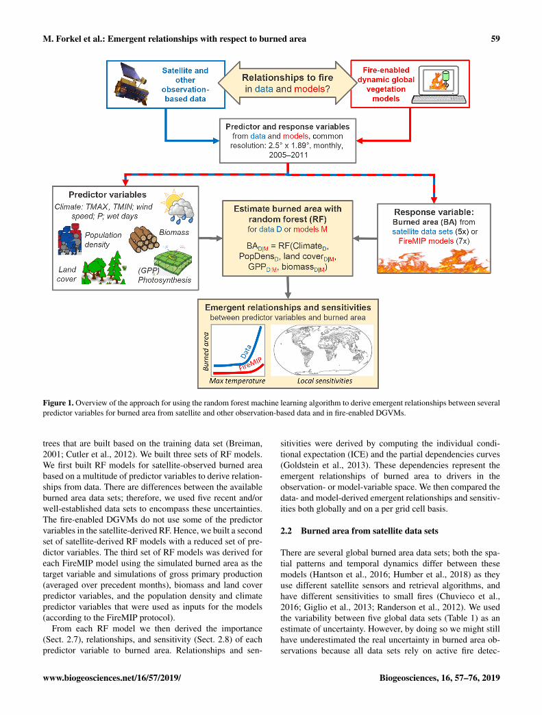
In order to infer relationships between potential drivers offire in satellite data and fire-enabled DGVMs, we appliedthe random forest (RF) machine-learning algorithm to pre-dict monthly burned area (response variable) from climate,vegetation, and socio-economic predictor variables (Fig. 1).Predictor variables and burned area were either taken fromsatellite and other observation-based data sets or from simu-lations by a suite of fire-enabled DGVMs from the Fire Mod-eling Intercomparison Project (FireMIP) (Rabin et al., 2017)to derive relationships for data sets and models, respectively.

The RF algorithm is a regression approach that allowsnon-linear, non-monotonic, and non-additive relations be-tween multiple predictor variables and the target variable.RF averages predicted values across an ensemble of decision

Biogeosciences, 16, 57–76, 2019 www.biogeosciences.net/16/57/2019/

M. Forkel et al.: Emergent relationships with respect to burned area 59

Figure 1. Overview of the approach for using the random forest machine learning algorithm to derive emergent relationships between severalpredictor variables for burned area from satellite and other observation-based data and in fire-enabled DGVMs.

trees that are built based on the training data set (Breiman,2001; Cutler et al., 2012). We built three sets of RF models.We first built RF models for satellite-observed burned areabased on a multitude of predictor variables to derive relation-ships from data. There are differences between the availableburned area data sets; therefore, we used five recent and/orwell-established data sets to encompass these uncertainties.The fire-enabled DGVMs do not use some of the predictorvariables in the satellite-derived RF. Hence, we built a secondset of satellite-derived RF models with a reduced set of pre-dictor variables. The third set of RF models was derived foreach FireMIP model using the simulated burned area as thetarget variable and simulations of gross primary production(averaged over precedent months), biomass and land coverpredictor variables, and the population density and climatepredictor variables that were used as inputs for the models(according to the FireMIP protocol).

From each RF model we then derived the importance(Sect. 2.7), relationships, and sensitivity (Sect. 2.8) of eachpredictor variable to burned area. Relationships and sen-

sitivities were derived by computing the individual condi-tional expectation (ICE) and the partial dependencies curves(Goldstein et al., 2013). These dependencies represent theemergent relationships of burned area to drivers in theobservation- or model-variable space. We then compared thedata- and model-derived emergent relationships and sensitiv-ities both globally and on a per grid cell basis.

2.2 Burned area from satellite data sets

There are several global burned area data sets; both the spa-tial patterns and temporal dynamics differ between thesemodels (Hantson et al., 2016; Humber et al., 2018) as theyuse different satellite sensors and retrieval algorithms, andhave different sensitivities to small fires (Chuvieco et al.,2016; Giglio et al., 2013; Randerson et al., 2012). We usedthe variability between five global data sets (Table 1) as anestimate of uncertainty. However, by doing so we might stillhave underestimated the real uncertainty in burned area ob-servations because all data sets rely on active fire detec-

www.biogeosciences.net/16/57/2019/ Biogeosciences, 16, 57–76, 2019


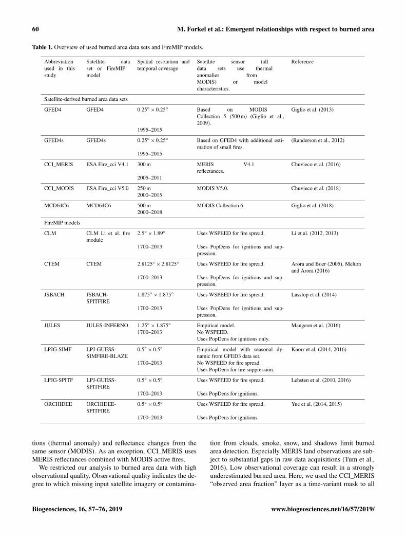
Table 1. Overview of used burned area data sets and FireMIP models.

Abbreviationused in thisstudy

Satellite dataset or FireMIPmodel

Spatial resolution andtemporal coverage

Satellite sensor (alldata sets use thermalanomalies fromMODIS) or modelcharacteristics.

Reference

Satellite-derived burned area data sets

GFED4 GFED4 0.25◦× 0.25◦ Based on MODISCollection 5 (500 m) (Giglio et al.,2009).

Giglio et al. (2013)

1995–2015

GFED4s GFED4s 0.25◦× 0.25◦ Based on GFED4 with additional esti-mation of small fires.

(Randerson et al., 2012)

1995–2015

CCI_MERIS ESA Fire_cci V4.1 300 m MERIS V4.1reflectances.

Chuvieco et al. (2016)

2005–2011

CCI_MODIS ESA Fire_cci V5.0 250 m MODIS V5.0. Chuvieco et al. (2018)2000–2015

MCD64C6 MCD64C6 500 m MODIS Collection 6. Giglio et al. (2018)2000–2018

FireMIP models

CLM CLM Li et al. firemodule

2.5◦× 1.89◦ Uses WSPEED for fire spread. Li et al. (2012, 2013)

1700–2013 Uses PopDens for ignitions and sup-pression.

CTEM CTEM 2.8125◦× 2.8125◦ Uses WSPEED for fire spread. Arora and Boer (2005), Meltonand Arora (2016)


JSBACH JSBACH-SPITFIRE

1.875◦× 1.875◦ Uses WSPEED for fire spread. Lasslop et al. (2014)


JULES JULES-INFERNO 1.25◦× 1.875◦ Empirical model. Mangeon et al. (2016)1700–2013 No WSPEED.

Uses PopDens for ignitions only.

LPJG-SIMF LPJ-GUESS-SIMFIRE-BLAZE

0.5◦× 0.5◦ Empirical model with seasonal dy-namic from GFED3 data set.

Knorr et al. (2014, 2016)

1700–2013 No WSPEED for fire spread.Uses PopDens for fire suppression.

LPJG-SPITF LPJ-GUESS-SPITFIRE

0.5◦× 0.5◦ Uses WSPEED for fire spread. Lehsten et al. (2010, 2016)

1700–2013 Uses PopDens for ignitions.

ORCHIDEE ORCHIDEE-SPITFIRE

0.5◦× 0.5◦ Uses WSPEED for fire spread. Yue et al. (2014, 2015)

1700–2013 Uses PopDens for ignitions.

tions (thermal anomaly) and reflectance changes from thesame sensor (MODIS). As an exception, CCI_MERIS usesMERIS reflectances combined with MODIS active fires.

We restricted our analysis to burned area data with highobservational quality. Observational quality indicates the de-gree to which missing input satellite imagery or contamina-

tion from clouds, smoke, snow, and shadows limit burnedarea detection. Especially MERIS land observations are sub-ject to substantial gaps in raw data acquisitions (Tum et al.,2016). Low observational coverage can result in a stronglyunderestimated burned area. Here, we used the CCI_MERIS“observed area fraction” layer as a time-variant mask to all



burned area data sets and only included estimates for monthswith observational coverage higher than 80 %. We also ex-cluded burned area in months with < 0 ◦C to remove sus-picious small burned areas in polar regions or in wintermonths which are likely caused by insufficiently correctedgas flares and other industrial activities. Analyses were madewith monthly burned area observations for the period from2005 to 2011, which is the common period between the fivedata sets.

2.3 Burned area from FireMIP models

A detailed description of FireMIP DGVMs and the simula-tion protocol is given by Rabin et al. (2017). Here we usedmonthly burned area from seven models that made transientsimulations from 1700 to 2013 (bottom half of Table 1). Themodels were forced using inputs of meteorological variablesfrom the CRUNCEP V5 data set (Wei et al., 2014), monthlycloud-to-ground lightning strikes (Rabin et al., 2017), annu-ally updated values of human population density from theHYDE 3.1 data set (Goldewijk et al., 2010), annually updatedland use and land cover changes from the Hurtt et al. (2011)data set, and annually updated values of global atmosphericCO2 (Le Quéré et al., 2014). Although forcing data sets arecommon across DGVMs, they do not use the same set offorcing variables, i.e. wind speed (WSPEED), or use popula-tion density (PopDens) for fire ignitions and/or fire suppres-sion.

The model outputs were aggregated to a common spa-tial resolution of 1.89◦ latitude×2.5◦ longitude. Aggregationwas undertaken by averaging the fractional burned area fromall high-resolution grid cells that belong to the same coarse-resolution grid cell. Nearest neighbour resampling was car-ried out if less than two high-resolution grid cells were withinone coarse-resolution grid cell. Analyses were also under-taken for the same period as the common window of thesatellite data (2005–2011) and by applying the “observedarea mask” from the satellite data.

2.4 Evaluation of data–data and model–data temporalagreement

We evaluated the temporal agreement of monthly burned areatime series for 2005–2011 between the data sets and betweenthe data sets and the fire-enabled DGVMs based on variousmodel performance metrics (Janssen and Heuberger, 1995)on a per-grid cell basis. We selected the Spearman rank corre-lation coefficient to compare the temporal agreement and thefractional variance (FV) to compare the variability of burnedarea per grid cells:

FV=σx − σref

0.5× (σx + σref), (1)

where σref and σx are the variances of the reference and ob-served or simulated burned area, respectively. FV ranges be-

tween −2 and 2 with negative values indicating an underes-timation and positive values indicating an overestimation ofthe observed variance. The reference ref is a vector of themonthly burned area time series from all satellite data sets:

ref = [BA.CCIMERIS, BA.CCIMODIS, BA.GFED4,BA.GFED4s, BA.MCD64C6]

In the case where a single satellite data set (e.g. x =BA.CCI_MERIS) was compared with the other satellite datasets, this data set was not used in the reference vector. Thisapproach directly considers the differences between data setsin the computation of model performance metrics and im-plies that it is impossible for a FireMIP model or for onesingle satellite data set to reach an optimal correlation ofunity or a FV of zero as long as the satellite burned areadata sets show differences. We used the median of the cor-relation coefficient and of the FV for each grid cell to quan-tify the data–data or model–data agreement over the ensem-ble of data sets or models. As a single global agreementmetric, we computed the percentage of the land area thatshowed “good” agreement from the spatial patterns of theSpearman correlation Cor and FV: good agreement for anindividual grid cell was defined based on a positive and non-random relationship (i.e. Cor≥ 0.25) and a comparable vari-ance (−0.75≤ FV≤ 0.75) between simulated and observedburned area.

2.5 Predictor variables and data sets

Several variables have been identified as predictors of globalfire in previous studies, inter alia the number of dry or wetdays per month (WET), diurnal temperature range (DTR),maximum temperature (TMAX), grass and shrub cover, leafarea index (LAI), net primary production (NPP), popula-tion density (PopDens), and gross domestic product (GDP)(Aldersley et al., 2011; Bistinas et al., 2014). Other variableshave been found important for fire at a regional scale, in-cluding total precipitation, tree cover, forest cover type, treeheight, biomass and litter fuel loads, and grazing (Archibaldet al., 2009; Chuvieco et al., 2014; Parisien et al., 2010; Pet-tinari and Chuvieco, 2017). We created a combined set of po-tential variables used in these studies to predict burned area(Table A1). We used data on gross primary production (GPP)instead of NPP as GPP can be estimated from eddy covari-ance observations and does not require model assumptionsabout autotrophic respiration.

2.5.1 Climate data

Climate data were taken from the CRUNCEP V5 data set(Wei et al., 2014). CRUNCEP provides 6-hourly time seriesof precipitation, maximum and minimum temperature, andwind speed. From these time series, we derived the monthlymean of daily maximum temperature (CRUNCEP.TMAX)and minimum temperature (CRUNCEP.TMIN), the monthly



mean daily diurnal temperature range (CRUNCEP.DTR=TMAX−TMIN), the monthly 90th percentile of daily windspeed (CRUNCEP.WSPEED), the monthly total precipita-tion (CRUNCEP.P), and the number of wet days per month(CRUNCEP.WET). A wet day was defined as a day with≥ 0.1 mm precipitation (Harris et al., 2014).

2.5.2 Land cover

Land cover was taken from the ESA CCI Land cover V2.0.7data set which provides annual land cover maps for the periodfrom 1992 to 2015 (Li et al., 2018). Land cover classes wereconverted into the fractional coverage of plant functionaltypes (PFTs). For this conversion, we used the cross-walkingapproach (Poulter et al., 2011, 2015) based on the conversiontable in Forkel et al. (2017). Individual PFTs combine growthform (tree, shrubs, herbaceous vegetation, or crops) with leaftype (broadleaved or needle-leaved) and leaf longevity (ever-green or deciduous). The variable Tree.BD, for example, isthe fractional coverage of broadleaved deciduous trees (Ta-ble A1). We created an additional category combining treesand shrubs (e.g. TreeS.BD= Tree.BD+Shrub.BD) becausemost of the FireMIP models simulate woody vegetationrather than separating shrubs and trees explicitly (Table S1in the Supplement). JULES, LPJG-SIMF, and LPJG-SPITFdynamically simulate the fractional coverage of PFTs, butCLM, CTEM, JSBACH, and ORCHIDEE used prescribedPFT distributions. We reclassified the PFTs of each modelinto the same set of PFTs that we derived from the CCI landcover data set (Table S1).

2.5.3 Vegetation productivity

Data on gross primary production (GPP) and leaf area index(LAI) were taken to account for the seasonal effects of vege-tation productivity and canopy development. GPP was takenfrom the FLUXCOM data set which is up-scaled from GPPestimates at FLUXNET measurement sites (Tramontana etal., 2016). We used the FLUXCOM data set that used satel-lite and CRUNCEP meteorological data for the upscaling.LAI was taken from MODIS (Myneni et al., 2015). GPP andLAI were averaged to monthly mean values (e.g. variablename GPP.orig). To account for seasonal fuel accumulation,we also computed previous-season GPP or LAI values as themean over the 3 and 6 months before the month of compari-son with burned area (e.g. GPP.pre3mon and GPP.pre6mon).

2.5.4 Biomass and fuels

We used temporally static vegetation data sets to account forthe effects of vegetation biomass, fuel properties, and ecosys-tem structure on burned area dynamics. Total above- andbelow-ground vegetation biomass was obtained from Carval-hais et al. (2014), which is based on an above-ground forestbiomass map for the tropics for the early 2000s (Saatchi etal., 2011), a total forest biomass map for temperate and bo-

real forests for the year 2010 (Thurner et al., 2014), and anestimate of herbaceous biomass (Carvalhais et al., 2014). Thevegetation biomass data set does not cover southern Australiaor New Zealand. Although fire is common in these regions,we did not fill the global vegetation biomass map with a re-gional map to avoid potential artefacts in the derived sensitiv-ities that would likely result from merging different biomassmaps. From each FireMIP model, we used the simulated veg-etation carbon averaged for the years from 2005 to 2011 asthe equivalent to this data set. We used canopy height fromSimard et al. (2011); this data set provides a snapshot ofthe average canopy height in 2005. Factors related to fuelproperties, specifically grass height, litter depth, woody litterdepth, and the amount of woody litter in different size classeswere extracted from the global fuel bed database (Pettinariand Chuvieco, 2016). This database is based on a land cover-based extrapolation of regional fuel databases for the globeand provides a generic picture of the conditions around 2005.

2.5.5 Socio-economic data

We used the annually varying population density data setfrom the HYDE V3.1 database (Klein Goldewijk et al.,2011), which was utilized as a forcing data set for theFireMIP simulations. We also used annually varying grossdomestic product per capita (GDP; World Bank, 2018), astatic satellite-derived index of socio-economic developmentbased on night-time lights for the year 2006 (Elvidge et al.,2012), and a data set on cattle density for the year 2007 (Wintand Robinson, 2007).

2.6 Random forest experiments and selection ofpredictor variables

We performed our analysis using the randomForest pack-age V4.6-12 in R (Liaw and Wiener, 2002). We trained theRF with 500 regression trees. The training target was eithera “satellite-observed” or a “model-simulated” burned area,i.e. we trained one RF against each burned area data set andeach individual FireMIP model simulation, respectively. Weused two sets of predictor variables in three sets of RF exper-iments (Table A1):

– “RF.Satellite.full” for satellite-derived RF experiments:we used 23 of the 28 predictor variables to train RFmodels for each burned area data set. Five predictorvariables were not included in the RF because theywere highly correlated with others (r > 0.8, i.e. night-light development index, cattle density, woody litter forthe 10 h fuel size class, precedent 3-monthly GPP, andprecedent 3-monthly LAI; Fig. S1 in the Supplement).The purpose of these experiments was to identify the re-lationship between burned area and each predictor vari-able from data sets.



– “RF.Satellite.fm” for satellite-derived RF experiments:these experiments were also trained against burned areadata sets but included only the reduced set of 16 data-based predictor variables that are available from bothobservational data sets and the FireMIP (fm) models.

– “RF.FireMIP.fm” for model-derived RF experiments:these experiments used the reduced set of predictor vari-ables with land cover, GPP, biomass, and the responsevariable burned area taken from simulations of eachFireMIP model. The purpose of these experiments wasto compare relationships and sensitivities from satellite-and FireMIP-derived RF experiments.

2.7 Importance of predictor variables in random forest

The normal method of determining the importance of predic-tor variables for RFs (increment in the mean-squared error –MSE) was found to be overly sensitive to the burnt area dataset that was used in training because of the highly skeweddistribution of burned area, and this hampers its interpretabil-ity (Figs. S8, S9). To overcome this issue and to obtain ad-ditional information about the regional (i.e. grid cell-level)importance of predictor variables, we developed an alterna-tive approach.

This alternative approach uses the fractional variance (FV)and Spearman correlation (r) instead of the MSE and is com-puted for each grid cell. The importance of variables is quan-tified as a distance D in a two-dimensional space based onthese metrics:

D =

√(0.5× (FVp−FV0)

)2+(rp− r0

)2, (2)

where FV0 and r0, and FVp and rp are the performance met-rics based on the original RF predictions and based on theRF predictions after permuting a single predictor variable,respectively. The FV-related term was multiplied by 0.5 toobtain the same range as the correlation. FV and r are com-puted at the grid cell-level based on the monthly burned areatime series from the RF predictions and the training data(i.e. burned area from a satellite data set or from a FireMIPmodel). As the metricD depends on the permutation, we per-mutated each predictor variable 10 times and averaged theDmetric.

2.8 Deriving emergent relationships and sensitivitiesfrom random forest

Insight into the shape of a relationship between a predictorand the target variable in a trained RF can be obtained frompartial dependence (PDP) (Friedman, 2001) and individualconditional expectation (ICE) plots (Goldstein et al., 2013;Fig. S2). PDPs show the partial relationship between the pre-dicted target variable and one predictor variable when otherpredictor variables are set to their mean value. ICE plotsshow the relationship between the predicted target variable

and one predictor variable for individual cases of the predic-tor data set (Goldstein et al., 2013). In our application, an in-dividual case is a specific combination of climate, land cover,vegetation, and socio-economic data for a given grid cell in agiven month (Fig. S2). The average of all ICE curves corre-sponds to the PDP. We used the ICEbox package V1.1.2 forR for the computation of ICE curves and partial dependen-cies (Goldstein et al., 2013).

We computed ICE curves for all predictor variables andfrom all RF experiments (Supplement Sects. S4 and S5). Wecomputed ICE curves and PDPs based on the global data setto analyse and compare global emergent relationships. ThePearson correlation coefficient was computed between pairsof satellite- and model-derived ICE curves to quantify theagreement of the emergent relationships (Fig. S15). We alsocomputed PDPs for each grid cell to produce global maps ofpartial sensitivities for selected predictor variables. To sum-marize and map the PDP of each grid cell in a single number,we fitted a linear quantile regression to the median betweenthe partial dependence of burned area and the correspondingpredictor variable and mapped the slope of this regression. Inthe following, we name this slope “sensitivity”.

3 Results

3.1 Evaluation of temporal burned area dynamics

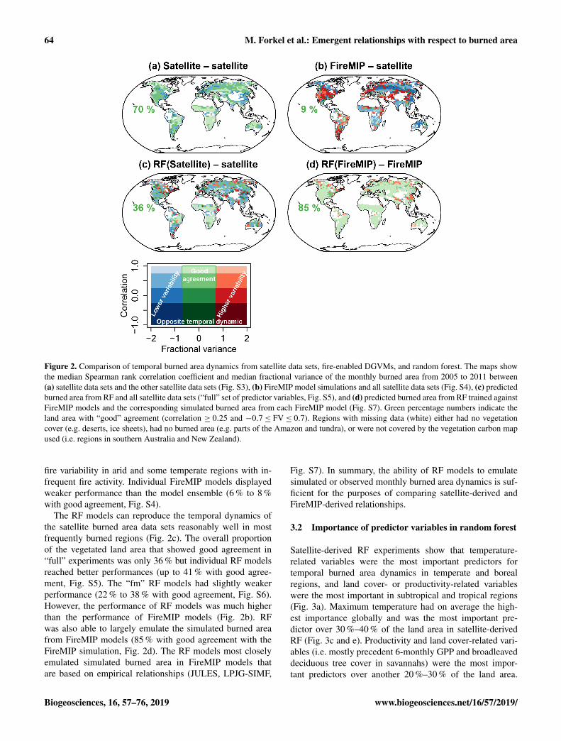
Here we compare the monthly temporal dynamics of burnedarea from the satellite data sets, FireMIP model simulations,and random forest predictions for the overlapping periodfrom 2005 to 2011. The satellite data sets showed relativelygood agreement with each other on average (i.e. “good” isr ≥ 0.25 and −0.7≤ FV≤ 0.7) over 70 % of the global veg-etated land area, with the best agreement found in frequentlyburning grasslands and savannahs (Fig. 2a). However, indi-vidual data sets only showed good agreement over 31 %–56 % of the land area (Fig. S3). The largest dissimilaritiesbetween burned area data sets occurred in temperate regionswith a high land use intensity (e.g. North America, Europe,China), tropical forests, and in sparsely vegetated arid andtundra regions. These difference are likely caused by limiteddetection possibilities under cloud cover (e.g. in the Amazon)and the sensitivities of the algorithms regarding the detectionof small fires (temperate and sparsely vegetated regions). Asthe CCI_MERIS data set is based on a different sensor, it isthe most different from the other data sets (31 % of land areashowed good agreement, Fig. S3). Hence, these uncertaintiesmake it necessary to separately train RF to each data set inorder to assess how such uncertainties translate into emergentrelationships to burned area.

FireMIP models showed good agreement with satellitedata sets over 9 % of the land area (Fig. 2b). In particu-lar, models tended to underestimate the variability of burnedarea in key biomass burning regions, while overestimating



Figure 2. Comparison of temporal burned area dynamics from satellite data sets, fire-enabled DGVMs, and random forest. The maps showthe median Spearman rank correlation coefficient and median fractional variance of the monthly burned area from 2005 to 2011 between(a) satellite data sets and the other satellite data sets (Fig. S3), (b) FireMIP model simulations and all satellite data sets (Fig. S4), (c) predictedburned area from RF and all satellite data sets (“full” set of predictor variables, Fig. S5), and (d) predicted burned area from RF trained againstFireMIP models and the corresponding simulated burned area from each FireMIP model (Fig. S7). Green percentage numbers indicate theland area with “good” agreement (correlation ≥ 0.25 and −0.7≤ FV≤ 0.7). Regions with missing data (white) either had no vegetationcover (e.g. deserts, ice sheets), had no burned area (e.g. parts of the Amazon and tundra), or were not covered by the vegetation carbon mapused (i.e. regions in southern Australia and New Zealand).

fire variability in arid and some temperate regions with in-frequent fire activity. Individual FireMIP models displayedweaker performance than the model ensemble (6 % to 8 %with good agreement, Fig. S4).

The RF models can reproduce the temporal dynamics ofthe satellite burned area data sets reasonably well in mostfrequently burned regions (Fig. 2c). The overall proportionof the vegetated land area that showed good agreement in“full” experiments was only 36 % but individual RF modelsreached better performances (up to 41 % with good agree-ment, Fig. S5). The “fm” RF models had slightly weakerperformance (22 % to 38 % with good agreement, Fig. S6).However, the performance of RF models was much higherthan the performance of FireMIP models (Fig. 2b). RFwas also able to largely emulate the simulated burned areafrom FireMIP models (85 % with good agreement with theFireMIP simulation, Fig. 2d). The RF models most closelyemulated simulated burned area in FireMIP models thatare based on empirical relationships (JULES, LPJG-SIMF,

Fig. S7). In summary, the ability of RF models to emulatesimulated or observed monthly burned area dynamics is suf-ficient for the purposes of comparing satellite-derived andFireMIP-derived relationships.

3.2 Importance of predictor variables in random forest

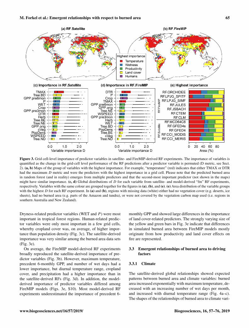
Satellite-derived RF experiments show that temperature-related variables were the most important predictors fortemporal burned area dynamics in temperate and borealregions, and land cover- or productivity-related variableswere the most important in subtropical and tropical regions(Fig. 3a). Maximum temperature had on average the high-est importance globally and was the most important pre-dictor over 30 %–40 % of the land area in satellite-derivedRF (Fig. 3c and e). Productivity and land cover-related vari-ables (i.e. mostly precedent 6-monthly GPP and broadleaveddeciduous tree cover in savannahs) were the most impor-tant predictors over another 20 %–30 % of the land area.



Figure 3. Grid cell-level importance of predictor variables in satellite- and FireMIP-derived RF experiments. The importance of variables isquantified as the change in the grid-cell level performance of the RF predictions after a predictor variable is permuted (D metric, see Sect.2). (a, b) Maps of the group of variables with the highest importance. For example, “temperature” (red) indicates that either TMAX or DTRhad the maximum D metric and were the predictors with the highest importance in a grid cell. Please note that the predicted burned areain random forest (and in reality) emerges from multiple predictors and that the second-most important predictor (not shown in the maps)might have similar importance. (c, d) Global distributions of D for each variable from satellite- and model-derived “fm” RF experiments,respectively. Variables with the same colour are grouped together for the figures in (a), (b), and (e). (e) Area distribution of the variable groupswith the highest D for each RF experiment. In (a) and (b), regions with missing data (white) either had no vegetation cover (e.g. deserts, icesheets), had no burned area (e.g. parts of the Amazon and tundra), or were not covered by the vegetation carbon map used (i.e. regions insouthern Australia and New Zealand).

Dryness-related predictor variables (WET and P ) were mostimportant in tropical forest regions. Human-related predic-tor variables were only most important in a few grid cells,whereby cropland cover was, on average, of higher impor-tance than population density (Fig. 3c). The satellite-derivedimportance was very similar among the burned area data sets(Fig. 3e).

On average, the FireMIP model-derived RF experimentsbroadly reproduced the satellite-derived importance of pre-dictor variables (Fig. 3b). However, maximum temperature,precedent 6-monthly GPP, and number of wet days had alower importance, but diurnal temperature range, croplandcover, and precipitation had a higher importance than inthe satellite-derived RFs (Fig. 3d). In addition, the model-derived importance of predictor variables differed amongFireMIP models (Figs. 3e, S10). Most model-derived RFexperiments underestimated the importance of precedent 6-

monthly GPP and showed large differences in the importanceof land cover-related predictors. The strongly varying size ofthe yellow and green bars in Fig. 3e indicate that differencesin simulated burned area between FireMIP models mostlyoriginate from how productivity and land cover effects onfire are represented.

3.3 Emergent relationships of burned area to drivingfactors

3.3.1 Climate

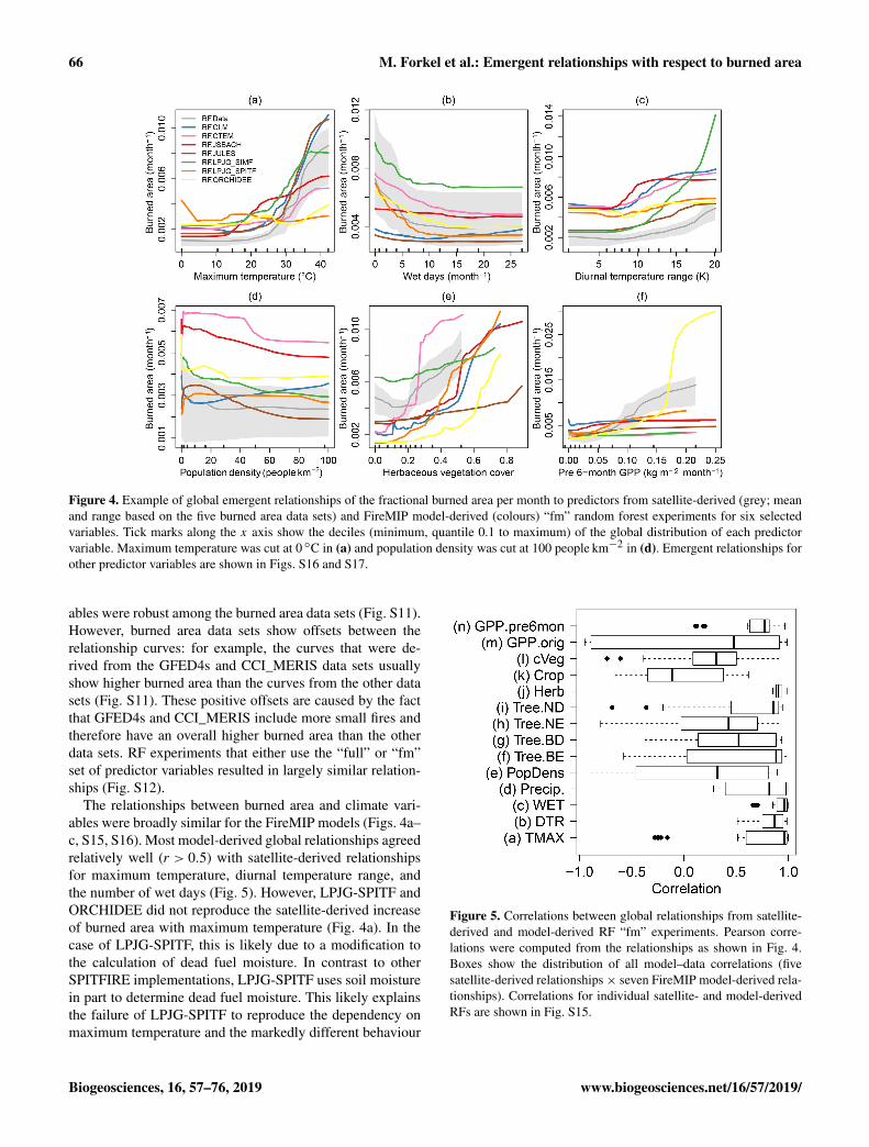
The satellite-derived global relationships showed expectedpatterns between burned area and climate variables: burnedarea increased exponentially with maximum temperature, de-creased with an increasing number of wet days per month,and increased with diurnal temperature range (Fig. 4a–c).The shapes of the relationships of burned area to climate vari-



Figure 4. Example of global emergent relationships of the fractional burned area per month to predictors from satellite-derived (grey; meanand range based on the five burned area data sets) and FireMIP model-derived (colours) “fm” random forest experiments for six selectedvariables. Tick marks along the x axis show the deciles (minimum, quantile 0.1 to maximum) of the global distribution of each predictorvariable. Maximum temperature was cut at 0 ◦C in (a) and population density was cut at 100 people km−2 in (d). Emergent relationships forother predictor variables are shown in Figs. S16 and S17.

ables were robust among the burned area data sets (Fig. S11).However, burned area data sets show offsets between therelationship curves: for example, the curves that were de-rived from the GFED4s and CCI_MERIS data sets usuallyshow higher burned area than the curves from the other datasets (Fig. S11). These positive offsets are caused by the factthat GFED4s and CCI_MERIS include more small fires andtherefore have an overall higher burned area than the otherdata sets. RF experiments that either use the “full” or “fm”set of predictor variables resulted in largely similar relation-ships (Fig. S12).

The relationships between burned area and climate vari-ables were broadly similar for the FireMIP models (Figs. 4a–c, S15, S16). Most model-derived global relationships agreedrelatively well (r > 0.5) with satellite-derived relationshipsfor maximum temperature, diurnal temperature range, andthe number of wet days (Fig. 5). However, LPJG-SPITF andORCHIDEE did not reproduce the satellite-derived increaseof burned area with maximum temperature (Fig. 4a). In thecase of LPJG-SPITF, this is likely due to a modification tothe calculation of dead fuel moisture. In contrast to otherSPITFIRE implementations, LPJG-SPITF uses soil moisturein part to determine dead fuel moisture. This likely explainsthe failure of LPJG-SPITF to reproduce the dependency onmaximum temperature and the markedly different behaviour

Figure 5. Correlations between global relationships from satellite-derived and model-derived RF “fm” experiments. Pearson corre-lations were computed from the relationships as shown in Fig. 4.Boxes show the distribution of all model–data correlations (fivesatellite-derived relationships× seven FireMIP model-derived rela-tionships). Correlations for individual satellite- and model-derivedRFs are shown in Fig. S15.



from the other SPITFIRE models seen here. CLM and JS-BACH did not reproduce the decrease in burned area withincreasing number of wet days (Fig. 4b).

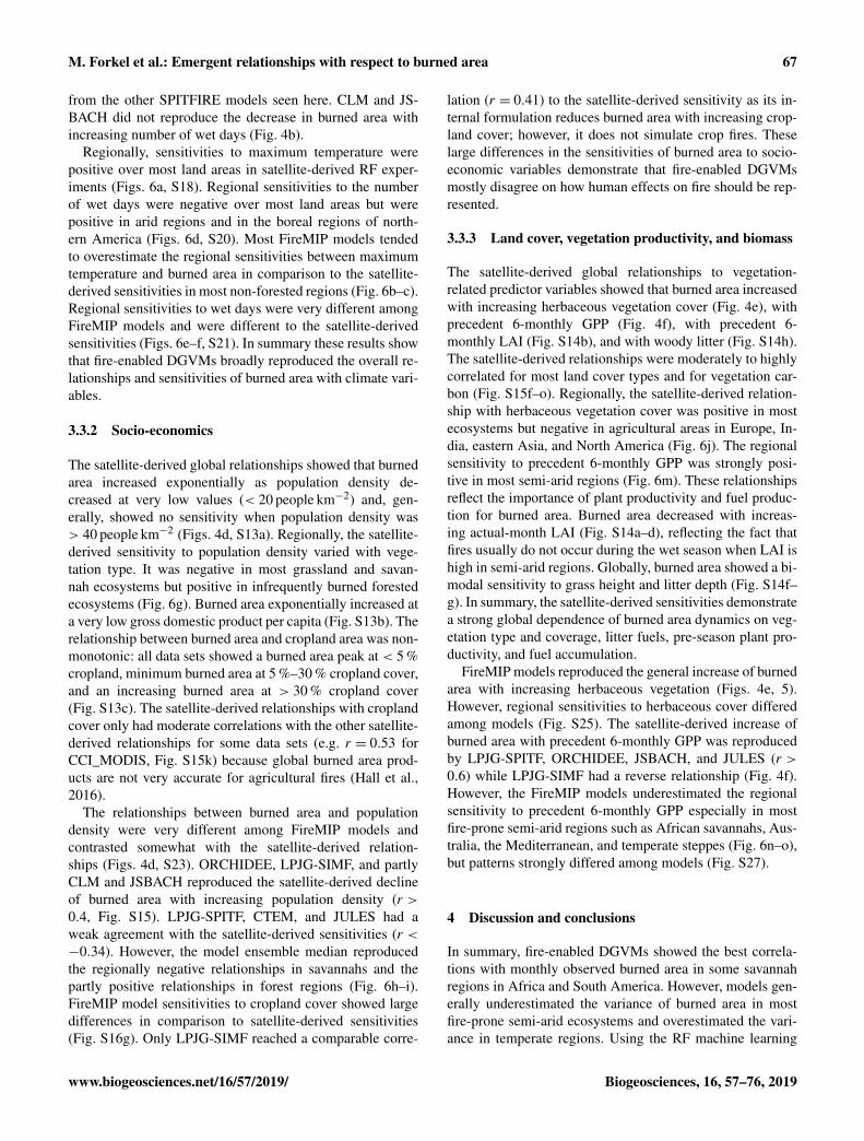
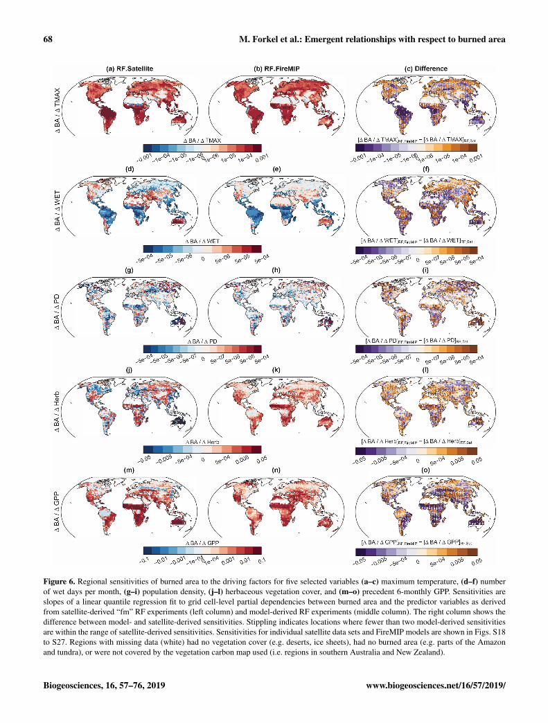
Regionally, sensitivities to maximum temperature werepositive over most land areas in satellite-derived RF exper-iments (Figs. 6a, S18). Regional sensitivities to the numberof wet days were negative over most land areas but werepositive in arid regions and in the boreal regions of north-ern America (Figs. 6d, S20). Most FireMIP models tendedto overestimate the regional sensitivities between maximumtemperature and burned area in comparison to the satellite-derived sensitivities in most non-forested regions (Fig. 6b–c).Regional sensitivities to wet days were very different amongFireMIP models and were different to the satellite-derivedsensitivities (Figs. 6e–f, S21). In summary these results showthat fire-enabled DGVMs broadly reproduced the overall re-lationships and sensitivities of burned area with climate vari-ables.

3.3.2 Socio-economics

The satellite-derived global relationships showed that burnedarea increased exponentially as population density de-creased at very low values (< 20 people km−2) and, gen-erally, showed no sensitivity when population density was> 40 people km−2 (Figs. 4d, S13a). Regionally, the satellite-derived sensitivity to population density varied with vege-tation type. It was negative in most grassland and savan-nah ecosystems but positive in infrequently burned forestedecosystems (Fig. 6g). Burned area exponentially increased ata very low gross domestic product per capita (Fig. S13b). Therelationship between burned area and cropland area was non-monotonic: all data sets showed a burned area peak at < 5 %cropland, minimum burned area at 5 %–30 % cropland cover,and an increasing burned area at > 30 % cropland cover(Fig. S13c). The satellite-derived relationships with croplandcover only had moderate correlations with the other satellite-derived relationships for some data sets (e.g. r = 0.53 forCCI_MODIS, Fig. S15k) because global burned area prod-ucts are not very accurate for agricultural fires (Hall et al.,2016).

The relationships between burned area and populationdensity were very different among FireMIP models andcontrasted somewhat with the satellite-derived relation-ships (Figs. 4d, S23). ORCHIDEE, LPJG-SIMF, and partlyCLM and JSBACH reproduced the satellite-derived declineof burned area with increasing population density (r >0.4, Fig. S15). LPJG-SPITF, CTEM, and JULES had aweak agreement with the satellite-derived sensitivities (r <−0.34). However, the model ensemble median reproducedthe regionally negative relationships in savannahs and thepartly positive relationships in forest regions (Fig. 6h–i).FireMIP model sensitivities to cropland cover showed largedifferences in comparison to satellite-derived sensitivities(Fig. S16g). Only LPJG-SIMF reached a comparable corre-

lation (r = 0.41) to the satellite-derived sensitivity as its in-ternal formulation reduces burned area with increasing crop-land cover; however, it does not simulate crop fires. Theselarge differences in the sensitivities of burned area to socio-economic variables demonstrate that fire-enabled DGVMsmostly disagree on how human effects on fire should be rep-resented.

3.3.3 Land cover, vegetation productivity, and biomass

The satellite-derived global relationships to vegetation-related predictor variables showed that burned area increasedwith increasing herbaceous vegetation cover (Fig. 4e), withprecedent 6-monthly GPP (Fig. 4f), with precedent 6-monthly LAI (Fig. S14b), and with woody litter (Fig. S14h).The satellite-derived relationships were moderately to highlycorrelated for most land cover types and for vegetation car-bon (Fig. S15f–o). Regionally, the satellite-derived relation-ship with herbaceous vegetation cover was positive in mostecosystems but negative in agricultural areas in Europe, In-dia, eastern Asia, and North America (Fig. 6j). The regionalsensitivity to precedent 6-monthly GPP was strongly posi-tive in most semi-arid regions (Fig. 6m). These relationshipsreflect the importance of plant productivity and fuel produc-tion for burned area. Burned area decreased with increas-ing actual-month LAI (Fig. S14a–d), reflecting the fact thatfires usually do not occur during the wet season when LAI ishigh in semi-arid regions. Globally, burned area showed a bi-modal sensitivity to grass height and litter depth (Fig. S14f–g). In summary, the satellite-derived sensitivities demonstratea strong global dependence of burned area dynamics on veg-etation type and coverage, litter fuels, pre-season plant pro-ductivity, and fuel accumulation.

FireMIP models reproduced the general increase of burnedarea with increasing herbaceous vegetation (Figs. 4e, 5).However, regional sensitivities to herbaceous cover differedamong models (Fig. S25). The satellite-derived increase ofburned area with precedent 6-monthly GPP was reproducedby LPJG-SPITF, ORCHIDEE, JSBACH, and JULES (r >0.6) while LPJG-SIMF had a reverse relationship (Fig. 4f).However, the FireMIP models underestimated the regionalsensitivity to precedent 6-monthly GPP especially in mostfire-prone semi-arid regions such as African savannahs, Aus-tralia, the Mediterranean, and temperate steppes (Fig. 6n–o),but patterns strongly differed among models (Fig. S27).

4 Discussion and conclusions

In summary, fire-enabled DGVMs showed the best correla-tions with monthly observed burned area in some savannahregions in Africa and South America. However, models gen-erally underestimated the variance of burned area in mostfire-prone semi-arid ecosystems and overestimated the vari-ance in temperate regions. Using the RF machine learning



Figure 6. Regional sensitivities of burned area to the driving factors for five selected variables (a–c) maximum temperature, (d–f) numberof wet days per month, (g–i) population density, (j–l) herbaceous vegetation cover, and (m–o) precedent 6-monthly GPP. Sensitivities areslopes of a linear quantile regression fit to grid cell-level partial dependencies between burned area and the predictor variables as derivedfrom satellite-derived “fm” RF experiments (left column) and model-derived RF experiments (middle column). The right column shows thedifference between model- and satellite-derived sensitivities. Stippling indicates locations where fewer than two model-derived sensitivitiesare within the range of satellite-derived sensitivities. Sensitivities for individual satellite data sets and FireMIP models are shown in Figs. S18to S27. Regions with missing data (white) had no vegetation cover (e.g. deserts, ice sheets), had no burned area (e.g. parts of the Amazonand tundra), or were not covered by the vegetation carbon map used (i.e. regions in southern Australia and New Zealand).



algorithm, we were able to diagnose reasons for these differ-ences between data and models: fire-enabled DGVMs largelyreproduced data-derived relationships and sensitivities be-tween burned area and climate variables. However, mod-els showed very different relationships with socio-economicvariables and generally underestimated sensitivities to pre-season plant productivity in all semi-arid ecosystems. As aconsequence, these results point towards fuel properties andfuel dynamics, and human–fire interactions as components offire-enabled DGVMs that should be the focus of future modeldevelopment. In the following, we will discuss methodolog-ical aspects of our applied pattern-oriented model evaluationapproach (Sect. 4.1), discuss controls on fire in data and mod-els (Sect. 4.2), and finally provide suggestions on how to im-prove fire-enabled DGVMs using current Earth observationdata sets (Sect. 4.3).

4.1 Pattern-oriented evaluation of DGVMs usingmachine learning

Simply speaking, simulations of fire (e.g. burned area) inDGVMs can be wrong because (1) the vegetation modelsimulates incorrect vegetation distributions, plant productiv-ity, and hence fuels, or (2) because the fire module mis-represents the response of fire to weather, humans, or fuelproperties. Classical model benchmarking uses, for exam-ple, maps of burned area, biomass, and tree cover to quan-tify the model–data mismatch between these variables (Kel-ley et al., 2013; Schaphoff et al., 2018). However, classi-cal model benchmarking does not allow one to disentanglethe individual effects of the vegetation or fire module on thesimulated burned area, as errors in the simulated vegetationmight be caused by errors in burned area and vice versa. Be-cause we use the same climate forcing, and vegetation statevariables derived from each model in our machine learningapproach, we are able to evaluate the response of fire mod-els independent of their underlying DGVMs. This allows usto derive (as partial dependencies or individual conditionalexpectations) and evaluate the relationships between predic-tors and the response for each fire module separately. Hence,we are able to attribute deficiencies in fire-enabled DGVMsto human- and productivity-influences on fire. Previously, asimilar approach also used a tree-based machine learning al-gorithm to evaluate drivers of soil carbon stocks in obser-vational databases and in Earth system models (Hashimotoet al., 2017). Unlike classical model benchmarking, suchpattern-oriented model evaluation approaches help to diag-nose the reasons for model–data mismatches.

The core of our pattern-oriented model evaluation is theapplication of a machine learning algorithm to learn emer-gent relationships from data or models. We used the randomforest algorithm because this algorithm has previously beenused to identify drivers of burned area (Aldersley et al., 2011;Archibald et al., 2009) and does not require any assump-tions about the statistical distribution of predictor variables,

the shape of relationships, or the interactions between pre-dictor variables, unlike algorithms such as generalized addi-tive/linear models (Bistinas et al., 2014; Forkel et al., 2017;Krawchuk et al., 2009). Other flexible algorithms such asmaximum entropy have also been used in empirical fire mod-elling (Moritz et al., 2012; Parisien et al., 2016) with verysimilar prediction performance and importance of variablescompared to random forest (Arpaci et al., 2014). In addition,the emergent relationships between predictors and burnedarea that we identified here show the same directions as therelationships that were found in a previous study based ongeneralized linear models (Bistinas et al., 2014). These find-ings suggest that the choice of machine learning algorithmonly marginally affects the direction and overall shape of thederived relationships.

4.2 Controls on burned area

Following previous studies, we found that climate is the pri-mary control of global burned area which directly affects firethrough weather and fuel moisture conditions, and indirectlythrough ecosystem productivity, vegetation type, and fuelloads (Archibald et al., 2013; Krawchuk and Moritz, 2011).Fire results from an interplay of several meteorological vari-ables, thereby maximum temperature is an important predic-tor globally – especially in northern temperate and borealecosystems. Fire-enabled DGVMs generally reproduced therelationships with maximum temperature but overestimatedthe sensitivity in grassland and savannah ecosystems on av-erage. Relationships and sensitivities with the number of wetdays showed larger differences among models and, whencompared to satellite-derived relationships, suggest that cli-mate effects on fuel moisture need to be improved in fire-enabled DGVMs.

As an indirect climate effect, we found that previous sea-son plant productivity was among the most important predic-tor variables globally and was the dominant predictor withthe strongest sensitivity to burned area in semi-arid savan-nah regions. It has long been recognized that the occurrenceand development of fires is affected by the production andaccumulation of fuels (Krawchuk and Moritz, 2011; Pausasand Ribeiro, 2013). Plant productivity in fire-prone semi-aridecosystems has a high year-to-year variability (Ahlström etal., 2015). Our results demonstrate that the inter-annual vari-ability in productivity and hence fuel accumulation is an im-portant driver of the variability in burned area. Most fire-enabled DGVMs poorly captured the importance, relation-ship, and sensitivity of previous-season plant productivity toburned area. This may be a reason why they underestimateobserved variability in burned area and why they misrepre-sent trends in fire occurrence in Africa as well as globally(Andela et al., 2017).

While climate and fuel controls when and where fires canburn, humans are responsible for the majority of fire igni-tions while also simultaneously suppressing fire. We found a



strong decline of burned area with increasing population den-sity between 0 and 20 people km−2 which confirms previousfindings (Bistinas et al., 2014; Knorr et al., 2014). Humaneffects on fire emerge from various activities such as tradi-tional land use practices (shifting cultivation, hunting, graz-ing, and grassland burning), the use of fires for land clear-ing or as tool in land conflicts, from prescribed small fireswithin fire management, and from unintended or illegal ig-nitions (Archibald, 2016; Bowman et al., 2011; Lauk andErb, 2009; van Marle et al., 2017). The modest performanceof random forest regarding reproducing satellite burned areasuggests that we did not capture the complexity of human–fire interactions with the set of predictor variables used. Forexample, the complex non-monotonic relationship betweenburned area and cropland cover suggests that agriculturalland use has diverging effects on fire in different agricul-tural regions of the world (Fig. S13c) (Korontzi et al., 2006).However, alternative variables such as cattle density or thenight light-based index of socio-economic development werehighly correlated with population density or cropland coverat the coarse resolution of our analysis; therefore, they didnot add to prediction performance of random forest. At re-gional scales, land use or infrastructure-related variables areimportant predictors for fire (Archibald et al., 2009; Arpaci etal., 2014; Chuvieco and Justice, 2010; Parisien et al., 2010).However, these regional findings also show that the impor-tance of human-related predictors largely differs between re-gions, which complicates its applicability for global-scalefire modelling. However, random forest largely emulated thesimulated burned area from FireMIP models, which suggeststhat we indeed included the main predictors for the modelworld. Although some newer global fire models include theeffects of cropland and pasture management on fires (Ra-bin et al., 2018), the complexity of human–fire interactionscurrently lacks a solid and large-scale empirical basis thatwould allow researchers to derive alternative formulations onhuman–fire interactions for fire-enabled DGVMs.

4.3 Improving vegetation controls on fire in DGVMs

Our results demonstrate that the role of vegetation on fireneeds to be better represented in fire-enabled DGVMs to ac-curately simulate the variability of burned area. The links be-tween vegetation productivity, fuel production, and fire needto be improved. Fuel production depends on plant productiv-ity, and on the allocation, turnover, and respiration processesof carbon in different fuel types. As a first step for model im-provement, fire-enabled DGVMs need to be tested and pos-sibly re-calibrated against observations or observation-basedestimates of plant productivity, above-ground biomass, andcarbon turnover (Carvalhais et al., 2014; Thurner et al., 2016,2017). Beyond total above-ground biomass, the evaluation ofdifferent fuel types (e.g. biomass in wood, canopy and un-derstory, and litter size classes) is currently hampered by theavailability of data. Only a few in situ measurements of fuel

loads exist (van Leeuwen et al., 2014) and global maps offuel properties are based on spatial extrapolations includingvarious assumptions and uncertainties (Pettinari and Chu-vieco, 2016). As an alternative, hybrid data–model-based ap-proaches such as land carbon cycle data assimilation systems(Bloom et al., 2016) may provide consistent information tobenchmark vegetation productivity, turnover, and litter fueldynamics in DGVMs.

Fire largely depends on the vegetation type (Rogers et al.,2015). Also our results show consistent land cover-specificrelationships to burned area in satellite data, but these rela-tionships differ among FireMIP models and in comparisonto the satellite-derived relationships (Fig. S17). Vegetationtypes and associated morphological, biochemical, and struc-tural characteristics of plants affect the flammability and firetolerance of vegetation (Archibald et al., 2018; Pausas et al.,2017). Although global fire models have PFT-specific param-eterizations for flammability (Thonicke et al., 2010), suchfire-relevant plant characteristics need to be incorporated inDGVMs (Zylstra et al., 2016). Such efforts should be com-plemented by calibrating DGVMs against satellite observa-tions that provide relevant information about the spatial dis-tributions of fuel structure (Pettinari and Chuvieco, 2016; Ri-año et al., 2002), fuel moisture content (Yebra et al., 2013,2018), fire ignitions and spread (Laurent et al., 2018), fuelconsumption (Andela et al., 2016), and fire radiative energy(Kaiser et al., 2012). In summary, besides human–fire inter-actions, we identified vegetation effects on fire as a main de-ficiency of fire-enabled dynamic global vegetation models insimulating temporal dynamics of burned area.

Code availability. This analysis is based on R (version 3.3.2) us-ing the randomForest (version 4.6-12) and ICEbox (version 1.1.2)packages. R and previously mentioned packages are available fromthe Comprehensive R Archive Network (CRAN, https://CRAN.R-project.org/package=randomForest (Breiman and Cutler, 2018);ICEbox, https://CRAN.R-project.org/package=ICEbox (Goldsteinet al., 2017), last access: 9 January 2019).

Data availability. Data are available from the references as indi-cated in Table A1.


https://CRAN.R-project.org/package=randomForest


https://CRAN.R-project.org/package=ICEbox


Appendix A

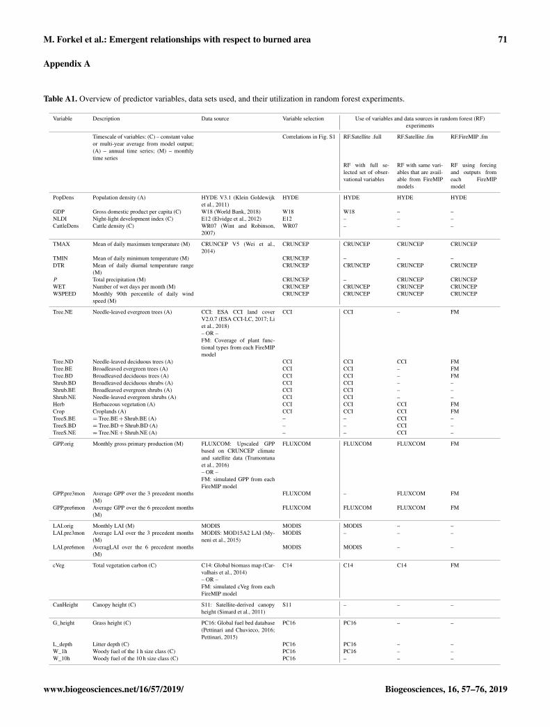
Table A1. Overview of predictor variables, data sets used, and their utilization in random forest experiments.

Variable Description Data source Variable selection Use of variables and data sources in random forest (RF)experiments

Timescale of variables: (C) – constant valueor multi-year average from model output;(A) – annual time series; (M) – monthlytime series

Correlations in Fig. S1 RF.Satellite .full RF.Satellite .fm RF.FireMIP .fm

RF with full se-lected set of obser-vational variables

RF with same vari-ables that are avail-able from FireMIPmodels

RF using forcingand outputs fromeach FireMIPmodel

PopDens Population density (A) HYDE V3.1 (Klein Goldewijket al., 2011)

HYDE HYDE HYDE HYDE

GDP Gross domestic product per capita (C) W18 (World Bank, 2018) W18 W18 – –NLDI Night-light development index (C) E12 (Elvidge et al., 2012) E12 – – –CattleDens Cattle density (C) WR07 (Wint and Robinson,

2007)WR07 – – –

TMAX Mean of daily maximum temperature (M) CRUNCEP V5 (Wei et al.,2014)

CRUNCEP CRUNCEP CRUNCEP CRUNCEP

TMIN Mean of daily minimum temperature (M) CRUNCEP – – –DTR Mean of daily diurnal temperature range

(M)CRUNCEP CRUNCEP CRUNCEP CRUNCEP

P Total precipitation (M) CRUNCEP – CRUNCEP CRUNCEPWET Number of wet days per month (M) CRUNCEP CRUNCEP CRUNCEP CRUNCEPWSPEED Monthly 90th percentile of daily wind

speed (M)CRUNCEP CRUNCEP CRUNCEP CRUNCEP

Tree.NE Needle-leaved evergreen trees (A) CCI: ESA CCI land coverV2.0.7 (ESA CCI-LC, 2017; Liet al., 2018)– OR –FM: Coverage of plant func-tional types from each FireMIPmodel

CCI CCI – FM

Tree.ND Needle-leaved deciduous trees (A) CCI CCI CCI FMTree.BE Broadleaved evergreen trees (A) CCI CCI – FMTree.BD Broadleaved deciduous trees (A) CCI CCI – FMShrub.BD Broadleaved deciduous shrubs (A) CCI CCI – –Shrub.BE Broadleaved evergreen shrubs (A) CCI CCI – –Shrub.NE Needle-leaved evergreen shrubs (A) CCI CCI – –Herb Herbaceous vegetation (A) CCI CCI CCI FMCrop Croplands (A) CCI CCI CCI FMTreeS.BE = Tree.BE+Shrub.BE (A) – – CCI –TreeS.BD = Tree.BD+Shrub.BD (A) – – CCI –TreeS.NE = Tree.NE+Shrub.NE (A) – – CCI –

GPP.orig Monthly gross primary production (M) FLUXCOM: Upscaled GPPbased on CRUNCEP climateand satellite data (Tramontanaet al., 2016)– OR –FM: simulated GPP from eachFireMIP model

FLUXCOM FLUXCOM FLUXCOM FM

GPP.pre3mon Average GPP over the 3 precedent months(M)

FLUXCOM – FLUXCOM FM

GPP.pre6mon Average GPP over the 6 precedent months(M)

FLUXCOM FLUXCOM FLUXCOM FM

LAI.orig Monthly LAI (M) MODIS MODIS MODIS – –LAI.pre3mon Average LAI over the 3 precedent months

(M)MODIS: MOD15A2 LAI (My-neni et al., 2015)

MODIS – – –

LAI.pre6mon AveragLAI over the 6 precedent months(M)

MODIS MODIS – –

cVeg Total vegetation carbon (C) C14: Global biomass map (Car-valhais et al., 2014)– OR –FM: simulated cVeg from eachFireMIP model

C14 C14 C14 FM

CanHeight Canopy height (C) S11: Satellite-derived canopyheight (Simard et al., 2011)

S11 – – –

G_height Grass height (C) PC16: Global fuel bed database(Pettinari and Chuvieco, 2016;Pettinari, 2015)

PC16 PC16 – –

L_depth Litter depth (C) PC16 PC16 – –W_1h Woody fuel of the 1 h size class (C) PC16 PC16 – –W_10h Woody fuel of the 10 h size class (C) PC16 – – –



Supplement. The supplement related to this article is availableonline at: https://doi.org/10.5194/bg-16-57-2019-supplement.

Author contributions. MForkel, NA, SPH, GL, and MvM designedthe analysis. MForkel, SPH, WD, and AA defined the overall struc-ture and scope of the manuscript. MForkel developed the analy-sis code and performed the computations. MForkel wrote the paperwith inputs from NA and SPH. GL, MForrest, SH, FL, JM, SS, andCY created the FireMIP model simulations and commented on thestudy design. EC and AH contributed and processed burned areadata sets and related quality layers. WD contributed with predictordata sets. All co-authors commented on the paper.

Competing interests. The authors declare that they have no conflictof interest.

Acknowledgements. We thank the institutions, initiatives, andresearchers listed in Table A1 for providing data sets. We thankStephane Mangeon for providing JULES-INFERNO model resultsto FireMIP. Matthias Forkel was supported by a Living Planet Fel-lowship from the European Space Agency, and Matthias Forkel andWouter Dorigo were funded by the TU Wien Wissenschaftspreis2015, a personal science award to Wouter Dorigo. Niels Andelareceived funding from the Gordon and Betty Moore Foundation(grant no. GBMF3269). The MERIS and MODIS Fire_CCI datasets were generated under the ESA Climate Change Initiative.Sandy P. Harrison acknowledges the support from the ERC-fundedproject GC2.0 (Global Change 2.0: Unlocking the past for a clearerfuture, grant number 694481). The authors acknowledge the TUWien University Library for financial support through its OpenAccess Funding Program.

Edited by: Paul StoyReviewed by: two anonymous referees

References

Ahlström, A., Raupach, M. R., Schurgers, G., Smith, B., Arneth,A., Jung, M., Reichstein, M., Canadell, J. G., Friedlingstein,P., Jain, A. K., Kato, E., Poulter, B., Sitch, S., Stocker, B. D.,Viovy, N., Wang, Y. P., Wiltshire, A., Zaehle, S., and Zeng,N.: The dominant role of semi-arid ecosystems in the trendand variability of the land CO2 sink, Science, 348, 895–899,https://doi.org/10.1126/science.aaa1668, 2015.

Aldersley, A., Murray, S. J., and Cornell, S. E.: Globaland regional analysis of climate and human driversof wildfire, Sci. Total Environ., 409, 3472–3481,https://doi.org/10.1016/j.scitotenv.2011.05.032, 2011.

Andela, N. and van der Werf, G. R.: Recent trends inAfrican fires driven by cropland expansion and El Ninoto La Nina transition, Nat. Clim. Change, 4, 791–795,https://doi.org/10.1038/nclimate2313, 2014.

Andela, N., van der Werf, G. R., Kaiser, J. W., van Leeuwen,T. T., Wooster, M. J., and Lehmann, C. E. R.: Biomass burn-ing fuel consumption dynamics in the tropics and subtrop-

ics assessed from satellite, Biogeosciences, 13, 3717–3734,https://doi.org/10.5194/bg-13-3717-2016, 2016.

Andela, N., Morton, D. C., Giglio, L., Chen, Y., van der Werf, G.R., Kasibhatla, P. S., DeFries, R. S., Collatz, G. J., Hantson, S.,Kloster, S., Bachelet, D., Forrest, M., Lasslop, G., Li, F., Man-geon, S., Melton, J. R., Yue, C., and Randerson, J. T.: A human-driven decline in global burned area, Science, 356, 1356–1362,https://doi.org/10.1126/science.aal4108, 2017.

Andreae, M. O. and Merlet, P.: Emission of trace gases and aerosolsfrom biomass burning, Global Biogeochem. Cy., 15, 955–966,https://doi.org/10.1029/2000GB001382, 2001.

Aragão, L. E. O. C., Anderson, L. O., Fonseca, M. G., Rosan, T.M., Vedovato, L. B., Wagner, F. H., Silva, C. V. J., Silva Ju-nior, C. H. L., Arai, E., Aguiar, A. P., Barlow, J., Berenguer, E.,Deeter, M. N., Domingues, L. G., Gatti, L., Gloor, M., Malhi,Y., Marengo, J. A., Miller, J. B., Phillips, O. L., and Saatchi,S.: 21st Century drought-related fires counteract the decline ofAmazon deforestation carbon emissions, Nat. Commun., 9, 536,https://doi.org/10.1038/s41467-017-02771-y, 2018.

Archibald, S.: Managing the human component of fire regimes:lessons from Africa, Phil. T. R. Soc. B, 371, 20150346,https://doi.org/10.1098/rstb.2015.0346, 2016.

Archibald, S., Roy, D. P., Van Wilgen, B. W., and Scholes,R. J.: What limits fire? An examination of drivers of burntarea in Southern Africa, Glob. Change Biol., 15, 613–630,https://doi.org/10.1111/j.1365-2486.2008.01754.x, 2009.

Archibald, S., Lehmann, C. E. R., Gómez-Dans, J. L., andBradstock, R. A.: Defining pyromes and global syndromesof fire regimes, P. Natl. Acad. Sci. USA, 110, 6442–6447,https://doi.org/10.1073/pnas.1211466110, 2013.

Archibald, S., Lehmann, C. E. R., Belcher, C. M., Bond, W. J., Brad-stock, R. A., Daniau, A.-L., Dexter, K. G., Forrestel, E. J., MGreve, He, T., Higgins, S. I., Hoffmann, W. A., Lamont, B. B.,McGlinn, D. J., Moncrieff, G. R., Osborne, C. P., Pausas, J. G.,O Price, Ripley, B. S., Rogers, B. M., Schwilk, D. W., Simon, M.F., Turetsky, M. R., van der Werf, G. R., and Zanne, A. E.: Bio-logical and geophysical feedbacks with fire in the Earth system,Environ. Res. Lett., 13, 033003, https://doi.org/10.1088/1748-9326/aa9ead, 2018.

Arora, V. K. and Boer, G. J.: Fire as an interactive componentof dynamic vegetation models, J. Geophys. Res.-Biogeo., 110,G02008, https://doi.org/10.1029/2005JG000042, 2005.

Arpaci, A., Malowerschnig, B., Sass, O., and Vacik, H.: Us-ing multi variate data mining techniques for estimating firesusceptibility of Tyrolean forests, Appl. Geogr., 53, 258–270,https://doi.org/10.1016/j.apgeog.2014.05.015, 2014.

Beck, P. S. A., Goetz, S. J., Mack, M. C., Alexander, H. D., Jin,Y., Randerson, J. T., and Loranty, M. M.: The impacts and im-plications of an intensifying fire regime on Alaskan boreal for-est composition and albedo, Glob. Change Biol., 17, 2853–2866,https://doi.org/10.1111/j.1365-2486.2011.02412.x, 2011.

Bistinas, I., Harrison, S. P., Prentice, I. C., and Pereira, J. M.C.: Causal relationships versus emergent patterns in the globalcontrols of fire frequency, Biogeosciences, 11, 5087–5101,https://doi.org/10.5194/bg-11-5087-2014, 2014.

Bloom, A. A., Exbrayat, J.-F., van der Velde, I. R., Feng, L.,and Williams, M.: The decadal state of the terrestrial carboncycle: Global retrievals of terrestrial carbon allocation, pools,


https://doi.org/10.5194/bg-16-57-2019-supplement

https://doi.org/10.1126/science.aaa1668

https://doi.org/10.1016/j.scitotenv.2011.05.032

https://doi.org/10.1038/nclimate2313

https://doi.org/10.5194/bg-13-3717-2016

https://doi.org/10.1126/science.aal4108

https://doi.org/10.1029/2000GB001382

https://doi.org/10.1038/s41467-017-02771-y

https://doi.org/10.1098/rstb.2015.0346

https://doi.org/10.1111/j.1365-2486.2008.01754.x

https://doi.org/10.1073/pnas.1211466110

https://doi.org/10.1088/1748-9326/aa9ead

https://doi.org/10.1088/1748-9326/aa9ead

https://doi.org/10.1029/2005JG000042

https://doi.org/10.1016/j.apgeog.2014.05.015

https://doi.org/10.1111/j.1365-2486.2011.02412.x

https://doi.org/10.5194/bg-11-5087-2014


and residence times, P. Natl. Acad. Sci. USA, 113, 1285–1290,https://doi.org/10.1073/pnas.1515160113, 2016.

Bond, W. J., Woodward, F. I., and Midgley, G. F.: Theglobal distribution of ecosystems in a world without fire,New Phytol., 165, 525–538, https://doi.org/10.1111/j.1469-8137.2004.01252.x, 2004.

Bowman, D. M. J. S., Balch, J. K., Artaxo, P., Bond, W. J., Carlson,J. M., Cochrane, M. A., D’Antonio, C. M., DeFries, R. S., Doyle,J. C., Harrison, S. P., Johnston, F. H., Keeley, J. E., Krawchuk,M. A., Kull, C. A., Marston, J. B., Moritz, M. A., Prentice, I. C.,Roos, C. I., Scott, A. C., Swetnam, T. W., van der Werf, G. R.,and Pyne, S. J.: Fire in the Earth System, Science, 324, 481–484,https://doi.org/10.1126/science.1163886, 2009.

Bowman, D. M. J. S., Balch, J., Artaxo, P., Bond, W. J., Cochrane,M. A., D’Antonio, C. M., DeFries, R., Johnston, F. H., Kee-ley, J. E., Krawchuk, M. A., Kull, C. A., Mack, M., Moritz, M.A., Pyne, S., Roos, C. I., Scott, A. C., Sodhi, N. S., and Swet-nam, T. W.: The human dimension of fire regimes on Earth,J. Biogeogr., 38, 2223–2236, https://doi.org/10.1111/j.1365-2699.2011.02595.x, 2011.

Breiman, L.: Random Forests, Mach. Learn., 45, 5–32,https://doi.org/10.1023/A:1010933404324, 2001.

Breiman, L. and Cutler, A.: randomForest: Breiman and Cutler’sRandom Forests for Classification and Regression, availableat: https://CRAN.R-project.org/package=randomForest (last ac-cess: 9 January 2019), 2018.

Carvalhais, N., Forkel, M., Khomik, M., Bellarby, J., Jung, M.,Migliavacca, M., Mu, M., Saatchi, S., Santoro, M., Thurner, M.,Weber, U., Ahrens, B., Beer, C., Cescatti, A., Randerson, J. T.,and Reichstein, M.: Global covariation of carbon turnover timeswith climate in terrestrial ecosystems, Nature, 514, 213–217,https://doi.org/10.1038/nature13731, 2014.

Chuvieco, E. and Justice, C.: Relations Between Human Fac-tors and Global Fire Activity, in: Advances in Earth Obser-vation of Global Change, edited by: Chuvieco, E., Li, J., andYang, X., 187–199, Springer, the Netherlands, Dordrecht, avail-able at: http://link.springer.com/10.1007/978-90-481-9085-0_14 (last access: 24 October 2016), 2010.

Chuvieco, E., Aguado, I., Jurdao, S., Pettinari, M. L., Yebra, M.,Salas, J., Hantson, S., de la Riva, J., Ibarra, P., Rodrigues, M.,Echeverría, M., Azqueta, D., Román, M. V., Bastarrika, A.,Martínez, S., Recondo, C., Zapico, E., and Vega, J. M.: Inte-grating geospatial information into fire risk assessment, Int. J.Wildland Fire, 23, 606, https://doi.org/10.1071/WF12052, 2014.

Chuvieco, E., Yue, C., Heil, A., Mouillot, F., Alonso-Canas,I., Padilla, M., Pereira, J. M., Oom, D., and Tansey, K.:A new global burned area product for climate assess-ment of fire impacts, Glob. Ecol. Biogeogr., 25, 619–629,https://doi.org/10.1111/geb.12440, 2016.

Chuvieco, E., Lizundia-Loiola, J., Pettinari, M. L., Ramo, R.,Padilla, M., Tansey, K., Mouillot, F., Laurent, P., Storm, T., Heil,A., and Plummer, S.: Generation and analysis of a new globalburned area product based on MODIS 250 m reflectance bandsand thermal anomalies, Earth Syst. Sci. Data, 10, 2015–2031,https://doi.org/10.5194/essd-10-2015-2018, 2018.

Cutler, A., Cutler, D. R., and Stevens, J. R.: Random Forests, inEnsemble Machine Learning, Springer, Boston, MA, 157–175,2012.

Elvidge, C. D., Baugh, K. E., Anderson, S. J., Sutton, P. C.,and Ghosh, T.: The Night Light Development Index (NLDI):a spatially explicit measure of human development from satel-lite data, Soc. Geogr., 7, 23–35, https://doi.org/10.5194/sg-7-23-2012, 2012.

ESA CCI-LC: Land Cover CCI Climate Research Data Package,available at: http://maps.elie.ucl.ac.be/CCI/viewer/download.php (last access: 5 February 2018), 2017.

Forkel, M., Dorigo, W., Lasslop, G., Teubner, I., Chuvieco, E.,and Thonicke, K.: A data-driven approach to identify con-trols on global fire activity from satellite and climate obser-vations (SOFIA V1), Geosci. Model Dev., 10, 4443–4476,https://doi.org/10.5194/gmd-10-4443-2017, 2017.

Friedman, J. H.: Greedy Function Approximation: A GradientBoosting Machine, Ann. Stat., 29, 1189–1232, 2001.

Giglio, L., Loboda, T., Roy, D. P., Quayle, B., and Justice, C. O.: Anactive-fire based burned area mapping algorithm for the MODISsensor, Remote Sens. Environ., 113, 408–420, 2009.

Giglio, L., Randerson, J. T., and van der Werf, G. R.: Analy-sis of daily, monthly, and annual burned area using the fourth-generation global fire emissions database (GFED4), J. Geophys.Res.-Biogeo., 118, 317–328, https://doi.org/10.1002/jgrg.20042,2013.

Giglio, L., Boschetti, L., Roy, D. P., Humber, M. L., and Jus-tice, C. O.: The Collection 6 MODIS burned area mappingalgorithm and product, Remote Sens. Environ., 217, 72–85,https://doi.org/10.1016/j.rse.2018.08.005, 2018.

Goldewijk, K. K., Beusen, A., and Janssen, P.: Long-term dy-namic modeling of global population and built-up area in aspatially explicit way: HYDE 3.1, Holocene, 20, 565–573,https://doi.org/10.1177/0959683609356587, 2010.

Goldstein, A., Kapelner, A., Bleich, J., and Pitkin, E.: Peeking In-side the Black Box: Visualizing Statistical Learning with Plotsof Individual Conditional Expectation, ArXiv13096392 Stat,available at: http://arxiv.org/abs/1309.6392 (last access: 26 June2017), 2013.

Goldstein, A., Kapelner, A., and Bleich, J.: ICEbox: Individual Con-ditional Expectation Plot Toolbox, available at: https://CRAN.R-project.org/package=ICEbox (last access: 9 January 2019),2017.

Hall, J. V., Loboda, T. V., Giglio, L., and McCarty, G. W.: AMODIS-based burned area assessment for Russian croplands:Mapping requirements and challenges, Remote Sens. Environ.,184, 506–521, https://doi.org/10.1016/j.rse.2016.07.022, 2016.

Hantson, S., Arneth, A., Harrison, S. P., Kelley, D. I., Prentice, I. C.,Rabin, S. S., Archibald, S., Mouillot, F., Arnold, S. R., Artaxo,P., Bachelet, D., Ciais, P., Forrest, M., Friedlingstein, P., Hickler,T., Kaplan, J. O., Kloster, S., Knorr, W., Lasslop, G., Li, F., Man-geon, S., Melton, J. R., Meyn, A., Sitch, S., Spessa, A., van derWerf, G. R., Voulgarakis, A., and Yue, C.: The status and chal-lenge of global fire modelling, Biogeosciences, 13, 3359–3375,https://doi.org/10.5194/bg-13-3359-2016, 2016.

Harris, I., Jones, P. D., Osborn, T. J., and Lister, D. H.: Up-dated high-resolution grids of monthly climatic observations– the CRU TS3.10 Dataset, Int. J. Climatol., 34, 623–642,https://doi.org/10.1002/joc.3711, 2014.

Harrison, S. P., Marlon, J., and Bartlein, P. J.: Fire in the Earth Sys-tem, in: Changing Climates, Earth Systems and Society, editedby: Dodson, J., Springer-Verlag, Dordrecht, 21–48, 2010.



https://doi.org/10.1111/j.1469-8137.2004.01252.x

https://doi.org/10.1111/j.1469-8137.2004.01252.x

https://doi.org/10.1126/science.1163886

https://doi.org/10.1111/j.1365-2699.2011.02595.x

https://doi.org/10.1111/j.1365-2699.2011.02595.x

https://doi.org/10.1023/A:1010933404324


https://doi.org/10.1038/nature13731

http://link.springer.com/10.1007/978-90-481-9085-0_14

http://link.springer.com/10.1007/978-90-481-9085-0_14

https://doi.org/10.1071/WF12052

https://doi.org/10.1111/geb.12440

https://doi.org/10.5194/essd-10-2015-2018

https://doi.org/10.5194/sg-7-23-2012

https://doi.org/10.5194/sg-7-23-2012

http://maps.elie.ucl.ac.be/CCI/viewer/download.php

http://maps.elie.ucl.ac.be/CCI/viewer/download.php

https://doi.org/10.5194/gmd-10-4443-2017

https://doi.org/10.1002/jgrg.20042

https://doi.org/10.1016/j.rse.2018.08.005

https://doi.org/10.1177/0959683609356587

http://arxiv.org/abs/1309.6392




https://doi.org/10.5194/bg-13-3359-2016

https://doi.org/10.1002/joc.3711


Hashimoto, S., Nanko, K., T̆upek, B., and Lehtonen, A.: Data-mining analysis of the global distribution of soil carbon inobservational databases and Earth system models, Geosci.Model Dev., 10, 1321–1337, https://doi.org/10.5194/gmd-10-1321-2017, 2017.

Holden, Z. A., Swanson, A., Luce, C. H., Jolly, W. M., Maneta,M., Oyler, J. W., Warren, D. A., Parsons, R., and Affleck, D.:Decreasing fire season precipitation increased recent western USforest wildfire activity, P. Natl. Acad. Sci. USA, 115, 201802316,https://doi.org/10.1073/pnas.1802316115, 2018.

Humber, M. L., Boschetti, L., Giglio, L., and Justice,C. O.: Spatial and temporal intercomparison of fourglobal burned area products, Int. J. Digit. Earth, 0, 1–25,https://doi.org/10.1080/17538947.2018.1433727, 2018.

Hurtt, G. C., Chini, L. P., Frolking, S., Betts, R. A., Feddema, J.,Fischer, G., Fisk, J. P., Hibbard, K., Houghton, R. A., Janetos,A., Jones, C. D., Kindermann, G., Kinoshita, T., Goldewijk, K.K., Riahi, K., Shevliakova, E., Smith, S., Stehfest, E., Thomson,A., Thornton, P., van Vuuren, D. P., and Wang, Y. P.: Harmo-nization of land-use scenarios for the period 1500–2100: 600years of global gridded annual land-use transitions, wood har-vest, and resulting secondary lands, Clim. Change, 109, 117,https://doi.org/10.1007/s10584-011-0153-2, 2011.

Janssen, P. H. M. and Heuberger, P. S. C.: Calibrationof process-oriented models, Ecol. Model., 83, 55–66,https://doi.org/10.1016/0304-3800(95)00084-9, 1995.

Jolly, W. M., Cochrane, M. A., Freeborn, P. H., Holden,Z. A., Brown, T. J., Williamson, G. J., and Bowman,D. M. J. S.: Climate-induced variations in global wild-fire danger from 1979 to 2013, Nat. Commun., 6, 7537,https://doi.org/10.1038/ncomms8537, 2015.

Kaiser, J. W., Heil, A., Andreae, M. O., Benedetti, A., Chubarova,N., Jones, L., Morcrette, J.-J., Razinger, M., Schultz, M. G.,Suttie, M., and van der Werf, G. R.: Biomass burning emis-sions estimated with a global fire assimilation system basedon observed fire radiative power, Biogeosciences, 9, 527–554,https://doi.org/10.5194/bg-9-527-2012, 2012.

Kelley, D. I., Prentice, I. C., Harrison, S. P., Wang, H., Simard, M.,Fisher, J. B., and Willis, K. O.: A comprehensive benchmarkingsystem for evaluating global vegetation models, Biogeosciences,10, 3313–3340, https://doi.org/10.5194/bg-10-3313-2013, 2013.

Klein Goldewijk, K., Beusen, A., van Drecht, G., and de Vos,M.: The HYDE 3.1 spatially explicit database of human-induced global land-use change over the past 12,000 years,Glob. Ecol. Biogeogr., 20, 73–86, https://doi.org/10.1111/j.1466-8238.2010.00587.x, 2011.

Knorr, W., Kaminski, T., Arneth, A., and Weber, U.: Impact of hu-man population density on fire frequency at the global scale,Biogeosciences, 11, 1085–1102, https://doi.org/10.5194/bg-11-1085-2014, 2014.

Knorr, W., Arneth, A., and Jiang, L.: Demographic controlsof future global fire risk, Nat. Clim. Change, 6, 781–785,https://doi.org/10.1038/nclimate2999, 2016.

Korontzi, S., McCarty, J., Loboda, T., Kumar, S., and Jus-tice, C.: Global distribution of agricultural fires in croplandsfrom 3 years of Moderate Resolution Imaging Spectroradiome-ter (MODIS) data, Global Biogeochem. Cy., 20, GB2021,https://doi.org/10.1029/2005GB002529, 2006.

Krawchuk, M. A. and Moritz, M. A.: Constraints on global fireactivity vary across a resource gradient, Ecology, 92, 121–132,https://doi.org/10.1890/09-1843.1, 2011.

Krawchuk, M. A., Moritz, M. A., Parisien, M.-A., Dorn, J.V., and Hayhoe, K.: Global Pyrogeography: the Currentand Future Distribution of Wildfire, PLOS ONE, 4, e5102,https://doi.org/10.1371/journal.pone.0005102, 2009.

Lasslop, G., Thonicke, K., and Kloster, S.: SPITFIREwithin the MPI Earth system model: Model developmentand evaluation, J. Adv. Model. Earth Syst., 6, 740–755,https://doi.org/10.1002/2013MS000284, 2014.

Lauk, C. and Erb, K.-H.: Biomass consumed in anthropogenic vege-tation fires: Global patterns and processes, Ecol. Econ., 69, 301–309, https://doi.org/10.1016/j.ecolecon.2009.07.003, 2009.

Laurent, P., Mouillot, F., Yue, C., Ciais, P., Moreno, M. V., andNogueira, J. M. P.: FRY, a global database of fire patch func-tional traits derived from space-borne burned area products, Sci.Data, 5, 180132, https://doi.org/10.1038/sdata.2018.132, 2018.

Lehsten, V., Harmand, P., Palumbo, I., and Arneth, A.: Mod-elling burned area in Africa, Biogeosciences, 7, 3199–3214,https://doi.org/10.5194/bg-7-3199-2010, 2010.

Lehsten, V., Arneth, A., Spessa, A., Thonicke, K., and Mous-takas, A.: The effect of fire on tree–grass coexistence in sa-vannas: a simulation study, Int. J. Wildland Fire, 25, 137,https://doi.org/10.1071/WF14205, 2016.

Le Quéré, C., Peters, G. P., Andres, R. J., Andrew, R. M., Boden,T. A., Ciais, P., Friedlingstein, P., Houghton, R. A., Marland, G.,Moriarty, R., Sitch, S., Tans, P., Arneth, A., Arvanitis, A., Bakker,D. C. E., Bopp, L., Canadell, J. G., Chini, L. P., Doney, S. C.,Harper, A., Harris, I., House, J. I., Jain, A. K., Jones, S. D., Kato,E., Keeling, R. F., Klein Goldewijk, K., Körtzinger, A., Koven,C., Lefèvre, N., Maignan, F., Omar, A., Ono, T., Park, G.-H.,Pfeil, B., Poulter, B., Raupach, M. R., Regnier, P., Rödenbeck, C.,Saito, S., Schwinger, J., Segschneider, J., Stocker, B. D., Taka-hashi, T., Tilbrook, B., van Heuven, S., Viovy, N., Wanninkhof,R., Wiltshire, A., and Zaehle, S.: Global carbon budget 2013,Earth Syst. Sci. Data, 6, 235–263, https://doi.org/10.5194/essd-6-235-2014, 2014.

Li, F. and Lawrence, D. M.: Role of Fire in the Global Land WaterBudget during the Twentieth Century due to Changing Ecosys-tems, J. Climate, 30, 1893–1908, https://doi.org/10.1175/JCLI-D-16-0460.1, 2016.

Li, F., Zeng, X. D., and Levis, S.: A process-based fireparameterization of intermediate complexity in a DynamicGlobal Vegetation Model, Biogeosciences, 9, 2761–2780,https://doi.org/10.5194/bg-9-2761-2012, 2012.

Li, F., Levis, S., and Ward, D. S.: Quantifying the role of fire inthe Earth system – Part 1: Improved global fire modeling in theCommunity Earth System Model (CESM1), Biogeosciences, 10,2293–2314, https://doi.org/10.5194/bg-10-2293-2013, 2013.

Li, W., MacBean, N., Ciais, P., Defourny, P., Lamarche, C., Bon-temps, S., Houghton, R. A., and Peng, S.: Gross and net landcover changes in the main plant functional types derived from theannual ESA CCI land cover maps (1992–2015), Earth Syst. Sci.Data, 10, 219–234, https://doi.org/10.5194/essd-10-219-2018,2018.

Liaw, A. and Wiener, M.: Classification and Regression by random-Forest, R News, 2, 18–22, 2002.


https://doi.org/10.5194/gmd-10-1321-2017

https://doi.org/10.5194/gmd-10-1321-2017


https://doi.org/10.1080/17538947.2018.1433727

https://doi.org/10.1007/s10584-011-0153-2

https://doi.org/10.1016/0304-3800(95)00084-9

https://doi.org/10.1038/ncomms8537

https://doi.org/10.5194/bg-9-527-2012

https://doi.org/10.5194/bg-10-3313-2013

https://doi.org/10.1111/j.1466-8238.2010.00587.x

https://doi.org/10.1111/j.1466-8238.2010.00587.x

https://doi.org/10.5194/bg-11-1085-2014

https://doi.org/10.5194/bg-11-1085-2014


https://doi.org/10.1029/2005GB002529

https://doi.org/10.1890/09-1843.1

https://doi.org/10.1371/journal.pone.0005102

https://doi.org/10.1002/2013MS000284

https://doi.org/10.1016/j.ecolecon.2009.07.003

https://doi.org/10.1038/sdata.2018.132

https://doi.org/10.5194/bg-7-3199-2010

https://doi.org/10.1071/WF14205



https://doi.org/10.1175/JCLI-D-16-0460.1

https://doi.org/10.1175/JCLI-D-16-0460.1

https://doi.org/10.5194/bg-9-2761-2012

https://doi.org/10.5194/bg-10-2293-2013



López-Saldaña, G., Bistinas, I., and Pereira, J. M. C.:Global analysis of radiative forcing from fire-inducedshortwave albedo change, Biogeosciences, 12, 557–565,https://doi.org/10.5194/bg-12-557-2015, 2015.

Mangeon, S., Voulgarakis, A., Gilham, R., Harper, A., Sitch, S., andFolberth, G.: INFERNO: a fire and emissions scheme for the UKMet Office’s Unified Model, Geosci. Model Dev., 9, 2685–2700,https://doi.org/10.5194/gmd-9-2685-2016, 2016.

Melton, J. R. and Arora, V. K.: Competition between plantfunctional types in the Canadian Terrestrial EcosystemModel (CTEM) v. 2.0, Geosci. Model Dev., 9, 323–361,https://doi.org/10.5194/gmd-9-323-2016, 2016.

Moritz, M. A., Parisien, M.-A., Batllori, E., Krawchuk, M. A.,Van Dorn, J., Ganz, D. J., and Hayhoe, K.: Climate changeand disruptions to global fire activity, Ecosphere, 3, 1–22,https://doi.org/10.1890/ES11-00345.1, 2012.

Müller, M., Vacik, H., and Valese, E.: Anomalies of theAustrian Forest Fire Regime in Comparison with OtherAlpine Countries: A Research Note, Forests, 6, 903–913,https://doi.org/10.3390/f6040903, 2015.

Myneni, R., Knyazikhin, Y., and Park, T.: MOD15A2 MODIS/TerraLeaf Area Index/FPAR 8-Day L4 Global 1km SIN Grid, BostonUniversity and MODAPS SIPS, NASA, NASA LP DAAC,https://doi.org/10.5067/MODIS/MOD15A2.006, 2015.

Parisien, M.-A., Parks, S. A., Krawchuk, M. A., Flannigan, M. D.,Bowman, L. M., and Moritz, M. A.: Scale-dependent controls onthe area burned in the boreal forest of Canada, 1980–2005, Ecol.Appl., 21, 789–805, https://doi.org/10.1890/10-0326.1, 2010.

Parisien, M.-A., Miller, C., Parks, S. A., DeLancey, E. R.,Robinne, F.-N., and Flannigan, M. D.: The spatially varyinginfluence of humans on fire probability in North America,Environ. Res. Lett., 11, 075005, https://doi.org/10.1088/1748-9326/11/7/075005, 2016.

Pausas, J. G. and Dantas, V. de L.: Scale matters: fire–vegetation feedbacks are needed to explain tropical treecover at the local scale, Glob. Ecol. Biogeogr., 26, 395–399,https://doi.org/10.1111/geb.12562, 2017.

Pausas, J. G. and Ribeiro, E.: The global fire–productivityrelationship, Glob. Ecol. Biogeogr., 22, 728–736,https://doi.org/10.1111/geb.12043, 2013.

Pausas, J. G., Keeley, J. E., and Schwilk, D. W.: Flammability asan ecological and evolutionary driver, J. Ecol., 105, 289–297,https://doi.org/10.1111/1365-2745.12691, 2017.

Pettinari, M. L.: Global Fuelbed Dataset, Department of Geology,Geography and Environment, University of Alcala, Spain, PAN-GAEA, https://doi.org/10.1594/PANGAEA.849808, 2015.

Pettinari, M. L. and Chuvieco, E.: Generation of a global fueldata set using the Fuel Characteristic Classification System,Biogeosciences, 13, 2061–2076, https://doi.org/10.5194/bg-13-2061-2016, 2016.

Pettinari, M. L. and Chuvieco, E.: Fire Behavior Simulationfrom Global Fuel and Climatic Information, Forests, 8, 179,https://doi.org/10.3390/f8060179, 2017.

Poulter, B., Ciais, P., Hodson, E., Lischke, H., Maignan, F., Plum-mer, S., and Zimmermann, N. E.: Plant functional type map-ping for earth system models, Geosci. Model Dev., 4, 993–1010,https://doi.org/10.5194/gmd-4-993-2011, 2011.

Poulter, B., MacBean, N., Hartley, A., Khlystova, I., Arino, O.,Betts, R., Bontemps, S., Boettcher, M., Brockmann, C., De-

fourny, P., Hagemann, S., Herold, M., Kirches, G., Lamarche, C.,Lederer, D., Ottlé, C., Peters, M., and Peylin, P.: Plant functionaltype classification for earth system models: results from the Eu-ropean Space Agency’s Land Cover Climate Change Initiative,Geosci. Model Dev., 8, 2315–2328, https://doi.org/10.5194/gmd-8-2315-2015, 2015.

Rabin, S. S., Melton, J. R., Lasslop, G., Bachelet, D., Forrest,M., Hantson, S., Kaplan, J. O., Li, F., Mangeon, S., Ward, D.S., Yue, C., Arora, V. K., Hickler, T., Kloster, S., Knorr, W.,Nieradzik, L., Spessa, A., Folberth, G. A., Sheehan, T., Voul-garakis, A., Kelley, D. I., Prentice, I. C., Sitch, S., Harrison,S., and Arneth, A.: The Fire Modeling Intercomparison Project(FireMIP), phase 1: experimental and analytical protocols withdetailed model descriptions, Geosci. Model Dev., 10, 1175–1197, https://doi.org/10.5194/gmd-10-1175-2017, 2017.

Rabin, S. S., Ward, D. S., Malyshev, S. L., Magi, B. I., Shevli-akova, E., and Pacala, S. W.: A fire model with distinct crop, pas-ture, and non-agricultural burning: use of new data and a model-fitting algorithm for FINAL.1, Geosci. Model Dev., 11, 815–842,https://doi.org/10.5194/gmd-11-815-2018, 2018.

Randerson, J. T., Liu, H., Flanner, M. G., Chambers, S. D., Jin, Y.,Hess, P. G., Pfister, G., Mack, M. C., Treseder, K. K., Welp, L. R.,Chapin Iii, F. S., Harden, J. W., Goulden, M. L., Lyons, E., Neff,J. C., Schuur, E. A. G., and Zender, C. S.: The Impact of Bo-real Forest Fire on Climate Warming, Science, 314, 1130–1132,2006.

Randerson, J. T., Chen, Y., van der Werf, G. R., Rogers, B. M., andMorton, D. C.: Global burned area and biomass burning emis-sions from small fires, J. Geophys. Res.-Biogeo., 117, G04012,https://doi.org/10.1029/2012JG002128, 2012.

Riaño, D., Chuvieco, E., Salas, J., Palacios-Orueta, A., and Bas-tarrika, A.: Generation of fuel type maps from Landsat TM im-ages and ancillary data in Mediterranean ecosystems, Can. J. For.Res., 32, 1301–1315, https://doi.org/10.1139/x02-052, 2002.

Rogers, B. M., Soja, A. J., Goulden, M. L., and Randerson, J.T.: Influence of tree species on continental differences in bo-real fires and climate feedbacks, Nat. Geosci., 8, 228–234,https://doi.org/10.1038/ngeo2352, 2015.

Saatchi, S. S., Harris, N. L., Brown, S., Lefsky, M., Mitchard,E. T. A., Salas, W., Zutta, B. R., Buermann, W., Lewis, S.L., Hagen, S., Petrova, S., White, L., Silman, M., and Morel,A.: Benchmark map of forest carbon stocks in tropical regionsacross three continents, P. Natl. Acad. Sci. USA, 108, 9899–9904, https://doi.org/10.1073/pnas.1019576108, 2011.

Schaphoff, S., Forkel, M., Müller, C., Knauer, J., von Bloh, W.,Gerten, D., Jägermeyr, J., Lucht, W., Rammig, A., Thonicke,K., and Waha, K.: LPJmL4 – a dynamic global vegetationmodel with managed land – Part 2: Model evaluation, Geosci.Model Dev., 11, 1377–1403, https://doi.org/10.5194/gmd-11-1377-2018, 2018.

Settele, J., Scholes, R. J., Betts, R., Bunn, S., Leadley, P., Nepstad,D. C., Overpeck, J. T., and Taboada, M. A.: Terrestrial and InlandWater Systems, in: Climate Change 2014 – Impacts, Adaptationand Vulnerability: Part A: Global and Sectoral Aspects: Work-ing Group II Contribution to the IPCC Fifth Assessment Report:Volume 1: Global and Sectoral Aspects, vol. 1, edited by: Inter-governmental Panel on Climate Change, Cambridge UniversityPress, Cambridge, 271–360, 2014.


https://doi.org/10.5194/bg-12-557-2015

https://doi.org/10.5194/gmd-9-2685-2016

https://doi.org/10.5194/gmd-9-323-2016

https://doi.org/10.1890/ES11-00345.1

https://doi.org/10.3390/f6040903

https://doi.org/10.5067/MODIS/MOD15A2.006

https://doi.org/10.1890/10-0326.1

https://doi.org/10.1088/1748-9326/11/7/075005

https://doi.org/10.1088/1748-9326/11/7/075005



https://doi.org/10.1111/1365-2745.12691

https://doi.org/10.1594/PANGAEA.849808

https://doi.org/10.5194/bg-13-2061-2016

https://doi.org/10.5194/bg-13-2061-2016

https://doi.org/10.3390/f8060179

https://doi.org/10.5194/gmd-4-993-2011

https://doi.org/10.5194/gmd-8-2315-2015

https://doi.org/10.5194/gmd-8-2315-2015

https://doi.org/10.5194/gmd-10-1175-2017

https://doi.org/10.5194/gmd-11-815-2018

https://doi.org/10.1029/2012JG002128

https://doi.org/10.1139/x02-052

https://doi.org/10.1038/ngeo2352


https://doi.org/10.5194/gmd-11-1377-2018

https://doi.org/10.5194/gmd-11-1377-2018


Simard, M., Pinto, N., Fisher, J. B., and Baccini, A.: Mapping forestcanopy height globally with spaceborne lidar, J. Geophys. Res.-Biogeo., 116, G04021, https://doi.org/10.1029/2011JG001708,2011.

Tepley, A. J., Thomann, E., Veblen, T. T., Perry, G. L. W.,Holz, A., Paritsis, J., Kitzberger, T., and Anderson-Teixeira,K. J.: Influences of fire-vegetation feedbacks and post-firerecovery rates on forest landscape vulnerability to alteredfire regimes, edited by: Lines, E., J. Ecol., 106, 1925–1940,https://doi.org/10.1111/1365-2745.12950, 2018.

Thonicke, K., Venevsky, S., Sitch, S., and Cramer, W.: The Role ofFire Disturbance for Global Vegetation Dynamics: Coupling Fireinto a Dynamic Global Vegetation Model, Glob. Ecol. Biogeogr.,10, 661–677, 2001.

Thonicke, K., Spessa, A., Prentice, I. C., Harrison, S. P., Dong,L., and Carmona-Moreno, C.: The influence of vegetation, firespread and fire behaviour on biomass burning and trace gas emis-sions: results from a process-based model, Biogeosciences, 7,1991–2011, https://doi.org/10.5194/bg-7-1991-2010, 2010.

Thurner, M., Beer, C., Santoro, M., Carvalhais, N., Wutzler, T.,Schepaschenko, D., Shvidenko, A., Kompter, E., Ahrens, B.,Levick, S. R., and Schmullius, C.: Carbon stock and density ofnorthern boreal and temperate forests, Glob. Ecol. Biogeogr., 23,297–310, https://doi.org/10.1111/geb.12125, 2014.

Thurner, M., Beer, C., Carvalhais, N., Forkel, M., San-toro, M., Tum, M., and Schmullius, C.: Large-scale vari-ation in boreal and temperate forest carbon turnover rateis related to climate, Geophys. Res. Lett., 43, 4576–4585,https://doi.org/10.1002/2016GL068794, 2016.

Thurner, M., Beer, C., Ciais, P., Friend, A. D., Ito, A., Kleidon,A., Lomas, M. R., Quegan, S., Rademacher, T. T., Schaphoff,S., Tum, M., Wiltshire, A., and Carvalhais, N.: Evaluation ofclimate-related carbon turnover processes in global vegetationmodels for boreal and temperate forests, Glob. Change Biol., 23,3076–3091, https://doi.org/10.1111/gcb.13660, 2017.

Tramontana, G., Jung, M., Schwalm, C. R., Ichii, K., Camps-Valls,G., Ráduly, B., Reichstein, M., Arain, M. A., Cescatti, A., Kiely,G., Merbold, L., Serrano-Ortiz, P., Sickert, S., Wolf, S., andPapale, D.: Predicting carbon dioxide and energy fluxes acrossglobal FLUXNET sites with regression algorithms, Biogeo-sciences, 13, 4291–4313, https://doi.org/10.5194/bg-13-4291-2016, 2016.

Tum, M., Günther, K., Böttcher, M., Baret, F., Bittner, M., Brock-mann, C., Weiss, M., Tum, M., Günther, K. P., Böttcher, M.,Baret, F., Bittner, M., Brockmann, C., and Weiss, M.: GlobalGap-Free MERIS LAI Time Series (2002–2012), Remote Sens.,8, 69, https://doi.org/10.3390/rs8010069, 2016.

van Leeuwen, T. T., van der Werf, G. R., Hoffmann, A. A., Det-mers, R. G., Rücker, G., French, N. H. F., Archibald, S., Car-valho Jr., J. A., Cook, G. D., de Groot, W. J., Hély, C., Kasischke,E. S., Kloster, S., McCarty, J. L., Pettinari, M. L., Savadogo,P., Alvarado, E. C., Boschetti, L., Manuri, S., Meyer, C. P.,Siegert, F., Trollope, L. A., and Trollope, W. S. W.: Biomassburning fuel consumption rates: a field measurement database,Biogeosciences, 11, 7305–7329, https://doi.org/10.5194/bg-11-7305-2014, 2014.

van Marle, M., Field, R. D., van der Werf, R. G., de Wagt,E. A. I., Houghton, R. A., Rizzo, L. V., Artaxo, P., andTsigaridis, K.: Fire and deforestation dynamics in Ama-

zonia (1973–2014), Global Biogeochem. Cy., 31, 24–38,https://doi.org/10.1002/2016GB005445, 2017.

Veraverbeke, S., Rogers, B. M., Goulden, M. L., Jandt, R.R., Miller, C. E., Wiggins, E. B., and Randerson, J. T.:Lightning as a major driver of recent large fire years inNorth American boreal forests, Nat. Clim. Change, 7, 529,https://doi.org/10.1038/nclimate3329, 2017.

Ward, D. S., Kloster, S., Mahowald, N. M., Rogers, B. M., Ran-derson, J. T., and Hess, P. G.: The changing radiative forcing offires: global model estimates for past, present and future, Atmos.Chem. Phys., 12, 10857–10886, https://doi.org/10.5194/acp-12-10857-2012, 2012.

Wei, Y., Liu, S., Huntzinger, D. N., Michalak, A. M., Viovy, N.,Post, W. M., Schwalm, C. R., Schaefer, K., Jacobson, A. R.,Lu, C., Tian, H., Ricciuto, D. M., Cook, R. B., Mao, J., andShi, X.: The North American Carbon Program Multi-scale Syn-thesis and Terrestrial Model Intercomparison Project – Part 2:Environmental driver data, Geosci. Model Dev., 7, 2875–2893,https://doi.org/10.5194/gmd-7-2875-2014, 2014.

Wint, W. and Robinson, T.: Gridded livestock of the world, FAO,Rome, 2007.

World Bank: GDP per capita (current US$), Data, available at:https://data.worldbank.org/indicator/NY.GDP.PCAP.CD?view=map, last access: 19 April 2018.

Yebra, M., Dennison, P. E., Chuvieco, E., Riaño, D., Zyl-stra, P., Hunt Jr., E. R., Danson, F. M., Qi, Y., and Ju-rdao, S.: A global review of remote sensing of live fuelmoisture content for fire danger assessment: Moving towardsoperational products, Remote Sens. Environ., 136, 455–468,https://doi.org/10.1016/j.rse.2013.05.029, 2013.

Yebra, M., Quan, X., Riaño, D., Rozas Larraondo, P., van Dijk, A.I. J. M., and Cary, G. J.: A fuel moisture content and flammabil-ity monitoring methodology for continental Australia based onoptical remote sensing, Remote Sens. Environ., 212, 260–272,https://doi.org/10.1016/j.rse.2018.04.053, 2018.

Yue, C., Ciais, P., Cadule, P., Thonicke, K., Archibald, S., Poul-ter, B., Hao, W. M., Hantson, S., Mouillot, F., Friedlingstein, P.,Maignan, F., and Viovy, N.: Modelling the role of fires in theterrestrial carbon balance by incorporating SPITFIRE into theglobal vegetation model ORCHIDEE – Part 1: simulating histor-ical global burned area and fire regimes, Geosci. Model Dev., 7,2747–2767, https://doi.org/10.5194/gmd-7-2747-2014, 2014.

Yue, C., Ciais, P., Cadule, P., Thonicke, K., and van Leeuwen, T.T.: Modelling the role of fires in the terrestrial carbon balance byincorporating SPITFIRE into the global vegetation model OR-CHIDEE – Part 2: Carbon emissions and the role of fires inthe global carbon balance, Geosci. Model Dev., 8, 1321–1338,https://doi.org/10.5194/gmd-8-1321-2015, 2015.

Zylstra, P., Bradstock, R. A., Bedward, M., Penman, T. D., Do-herty, M. D., Weber, R. O., Gill, A. M., and Cary, G. J.: Bio-physical Mechanistic Modelling Quantifies the Effects of PlantTraits on Fire Severity: Species, Not Surface Fuel Loads, Deter-mine Flame Dimensions in Eucalypt Forests, PLOS ONE, 11,e0160715, https://doi.org/10.1371/journal.pone.0160715, 2016.


https://doi.org/10.1029/2011JG001708

https://doi.org/10.1111/1365-2745.12950

https://doi.org/10.5194/bg-7-1991-2010


https://doi.org/10.1002/2016GL068794

https://doi.org/10.1111/gcb.13660

https://doi.org/10.5194/bg-13-4291-2016

https://doi.org/10.5194/bg-13-4291-2016

https://doi.org/10.3390/rs8010069

https://doi.org/10.5194/bg-11-7305-2014

https://doi.org/10.5194/bg-11-7305-2014

https://doi.org/10.1002/2016GB005445


https://doi.org/10.5194/acp-12-10857-2012

https://doi.org/10.5194/acp-12-10857-2012

https://doi.org/10.5194/gmd-7-2875-2014

https://data.worldbank.org/indicator/NY.GDP.PCAP.CD?view=map

https://data.worldbank.org/indicator/NY.GDP.PCAP.CD?view=map



https://doi.org/10.5194/gmd-7-2747-2014

https://doi.org/10.5194/gmd-8-1321-2015

https://doi.org/10.1371/journal.pone.0160715

Documents

Emergent relationships on burned area in global satellite