Embed Size (px)
Citation preview
Kota Miura
EMBL-CMCI course I
Basics of Image Processing andAnalysis
ver 2.1.1
Centre for Molecular & Cellular ImagingEMBL Heidelberg
Abstract
Aim: students acquire basic knowledge and techniques for handling dig-ital image data by interactively using ImageJ.
NOTE: this textbook was written using the Fiji distribution of ImageJ (IJver 1.47n, JRE 1.6.0_45). Exercises are recommended to be done using Fijisince most of plugins used in exercises are pre-installed in Fiji.
Many texts, images and exercises especially for chapter 1.3 and 1.4 wereconverted from the textbook of Matlab Image Processing Course in MBL,Woods Hall (which are originally from a book Digital Image Processing usingMatlab, Gonzalez et al, Prentice Hall). I thank Ivan Yudushkin for providingme with the manual he used there. Deconvolution tutorial was written byAlessandra Griffa and appears in this textbook with her kind acceptanceto do so. Figures on stack editing are drawn by Sébastien Toshi for hiscourse and appear in this textbook for his kind offer. I am pretty muchthankful to his figure and am impressed with the way he summarized allthe commands related to this. Sébastien Toshi also reviewed the article indetail and made may suggestions to improve the text. I thank him a lot forhis effort.
This text is progressively edited. Please ask me when you want to dis-tribute.
Compiled on: November 21, 2013Copyright 2006 - 2013, Kota Miura (http://cmci.embl.de)
Contents
1.1 Basics of Basics . . . . . . . . . . . . . . . . . . . . . . . . . . 4
1.1.1 Digital image is a matrix of numbers . . . . . . . . . . 4
1.1.2 Image Bit-Depth . . . . . . . . . . . . . . . . . . . . . 7
1.1.3 Converting the bit-depth of an image . . . . . . . . . 10
1.1.4 Math functions . . . . . . . . . . . . . . . . . . . . . . 14
1.1.5 Image Math . . . . . . . . . . . . . . . . . . . . . . . . 17
1.1.6 RGB image . . . . . . . . . . . . . . . . . . . . . . . . 18
1.1.7 Look-Up Table . . . . . . . . . . . . . . . . . . . . . . 24
1.1.8 Image File Formats . . . . . . . . . . . . . . . . . . . . 27
1.1.9 Multidimensional data . . . . . . . . . . . . . . . . . . 29
1.1.10 Command Finder . . . . . . . . . . . . . . . . . . . . . 40
1.1.11 Visualization of Multidimensional Images . . . . . . 41
1.1.12 Resampling images (Shrinking and Enlarging) . . . . 47
1.1.13 ASSIGNMENTS . . . . . . . . . . . . . . . . . . . . . 50
1.2 Intensity . . . . . . . . . . . . . . . . . . . . . . . . . . . . . . 52
1.2.1 Histogram . . . . . . . . . . . . . . . . . . . . . . . . . 52
1.2.2 Region of Interest (ROI) . . . . . . . . . . . . . . . . . 55
1.2.3 Intensity Measurement . . . . . . . . . . . . . . . . . . 56
1.2.4 Image transformation: Enhancing Contrast . . . . . . 59
EMBL CMCI ImageJ Basic Course CONTENTS
1.2.5 Image correlation between two images: co-localizationplot . . . . . . . . . . . . . . . . . . . . . . . . . . . . . 61
1.2.6 ASSIGNMENTS . . . . . . . . . . . . . . . . . . . . . 62
1.3 Filtering . . . . . . . . . . . . . . . . . . . . . . . . . . . . . . 63
1.3.1 Convolution . . . . . . . . . . . . . . . . . . . . . . . . 63
1.3.2 Kernels . . . . . . . . . . . . . . . . . . . . . . . . . . . 67
1.3.3 Morphological Image Processing . . . . . . . . . . . . 72
1.3.4 Morphological processing: Opening and Closing . . 76
1.3.5 Morphological Image Processing: Gray Scale Images 77
1.3.6 Background Subtraction . . . . . . . . . . . . . . . . . 78
1.3.7 Other Functions: Fill holes, Skeltonize, Outline . . . . 80
1.3.8 Batch Processing Files . . . . . . . . . . . . . . . . . . 81
1.3.9 Fast Fourier Transform (FFT) of Image . . . . . . . . . 83
1.3.10 Frequency-domain Convolution . . . . . . . . . . . . 87
1.3.11 Frequency-domain Filtering . . . . . . . . . . . . . . . 90
1.3.12 ASSIGNMENTS . . . . . . . . . . . . . . . . . . . . . 94
1.4 Segmentation . . . . . . . . . . . . . . . . . . . . . . . . . . . 95
1.4.1 Thresholding . . . . . . . . . . . . . . . . . . . . . . . 95
1.4.2 Feature Extraction - Edge Detection . . . . . . . . . . 100
1.4.3 Morphological Watershed . . . . . . . . . . . . . . . . 103
1.4.4 Particle Analysis . . . . . . . . . . . . . . . . . . . . . 105
1.4.5 Machine Learning: Trainable Segmentation . . . . . . 108
1.4.6 ASSIGNMENTS . . . . . . . . . . . . . . . . . . . . . 112
1.5 Analysis of Time Series . . . . . . . . . . . . . . . . . . . . . 115
1.5.1 Difference Images . . . . . . . . . . . . . . . . . . . . . 115
2
EMBL CMCI ImageJ Basic Course CONTENTS
1.5.2 Projection of Time Series . . . . . . . . . . . . . . . . . 116
1.5.3 Measurement of Intensity dynamics . . . . . . . . . . 117
1.5.4 Measurement of Movement Dynamics . . . . . . . . . 117
1.5.5 Kymographs . . . . . . . . . . . . . . . . . . . . . . . 118
1.5.6 Manual Tracking . . . . . . . . . . . . . . . . . . . . . 121
1.5.7 Automatic Tracking . . . . . . . . . . . . . . . . . . . 123
1.5.8 Summarizing the Tracking data . . . . . . . . . . . . . 129
1.5.9 ASSIGNMENTS . . . . . . . . . . . . . . . . . . . . . 132
References . . . . . . . . . . . . . . . . . . . . . . . . . . . . . . . . 133
1.6 Appendices . . . . . . . . . . . . . . . . . . . . . . . . . . . . 139
1.6.1 App.1 Header Structure and Image Files . . . . . . . 139
1.6.2 App.1.5 Installing Plug-In . . . . . . . . . . . . . . . . 140
1.6.3 App.1.75 List of accompanying PDF . . . . . . . . . . 141
1.6.4 App.2 Measurement Options . . . . . . . . . . . . . . 142
1.6.5 App.3 Edge Detection Principle . . . . . . . . . . . . 147
1.6.6 App.4 Particle Tracker manual . . . . . . . . . . . . . 149
1.6.7 App.5 Particle Analysis . . . . . . . . . . . . . . . . . 163
1.6.8 App.6 Image Processing and Analysis: software, script-ing language . . . . . . . . . . . . . . . . . . . . . . . . 165
1.6.9 App.7 Macro for Generating Striped images . . . . . 167
1.6.10 App.8 Deconvolution Exercise . . . . . . . . . . . . . 168
3
EMBL CMCI ImageJ Basic Course 1.1 Basics of Basics
1.1 Basics of Basics
Handling of digital images in scientific research requires knowledge on thecharacteristics of digital images. A digital image translates to numbers andis hence a quantitative signal by nature. In this section, we learn the verybasics of the numerical nature of digital images. Inappropriate handlingnot only lowers the quality of your analysis, but it could also be possiblethat your processing is considered as a "manipulation of data". For this lat-ter point, please also refer to Rossner and Yamada (2004). There are somelimits on acceptable image processing to maintain the scientific validity.Standards on scientific image processing could be found in "Digital Imag-ing: Ethics" by Cromey (2007).
1.1.1 Digital image is a matrix of numbers
A digital image we display on a computer screen is made up of pixels. Wecan see individual pixel by zooming up the image using the magnifyingtool1. Width and height of the image are defined by the number of pixels inx and y directions. Each pixel has brightness, or intensity (or more strictly,amplitude) somewhere between black and white represented as a number.Within an image file saved in a computer hard disk, the intensity valueof each pixels are written. The value is converted to the grayness of thatpixel on monitor screen. We usually do not see these values, or numbers,in the image displayed on monitor, but we could access these numbers inthe image file by converting the image file to a text file 2.
Exercise 1.1.1-1
Conversion of image to a text file
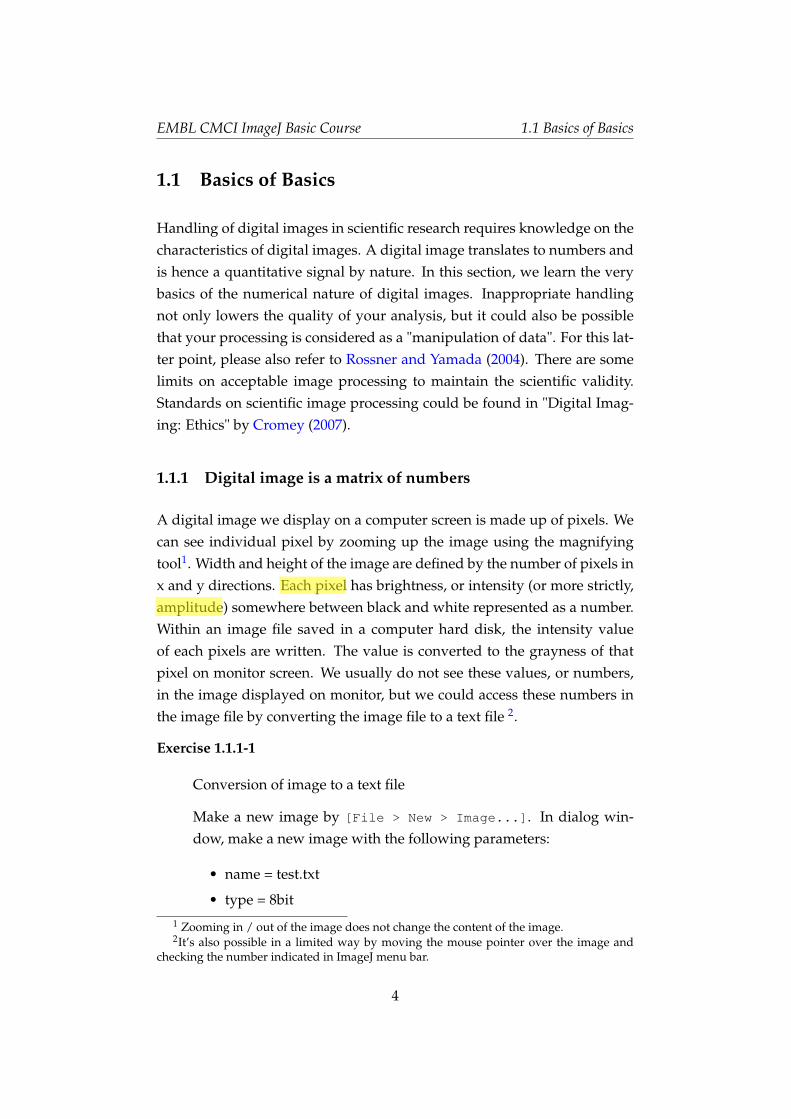
Make a new image by [File > New > Image...]. In dialog win-dow, make a new image with the following parameters:
• name = test.txt
• type = 8bit1 Zooming in / out of the image does not change the content of the image.2It’s also possible in a limited way by moving the mouse pointer over the image and
checking the number indicated in ImageJ menu bar.
4
EMBL CMCI ImageJ Basic Course 1.1 Basics of Basics
• Fill with Black
• 10 pixel width
• 15 pixel height
• Slices = 1
Figure 1.1 – New Image Dialog
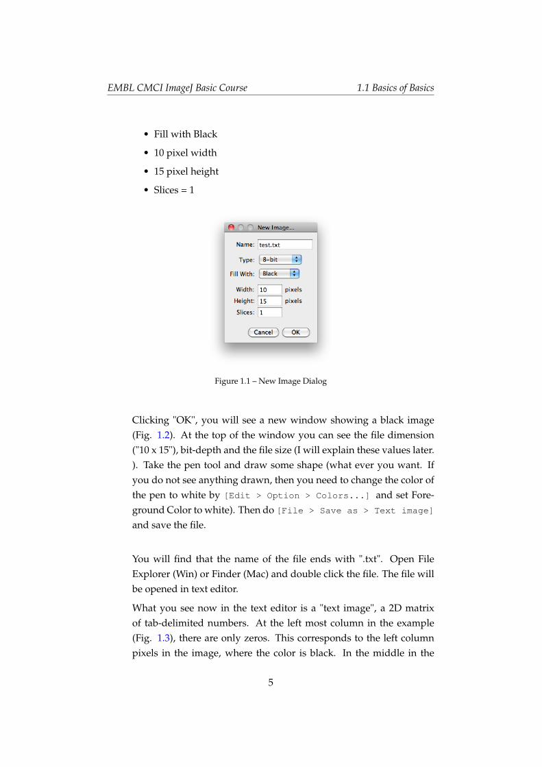
Clicking "OK", you will see a new window showing a black image(Fig. 1.2). At the top of the window you can see the file dimension("10 x 15"), bit-depth and the file size (I will explain these values later.). Take the pen tool and draw some shape (what ever you want. Ifyou do not see anything drawn, then you need to change the color ofthe pen to white by [Edit > Option > Colors...] and set Fore-ground Color to white). Then do [File > Save as > Text image]
and save the file.
You will find that the name of the file ends with ".txt". Open FileExplorer (Win) or Finder (Mac) and double click the file. The file willbe opened in text editor.
What you see now in the text editor is a "text image", a 2D matrixof tab-delimited numbers. At the left most column in the example(Fig. 1.3), there are only zeros. This corresponds to the left columnpixels in the image, where the color is black. In the middle in the
5
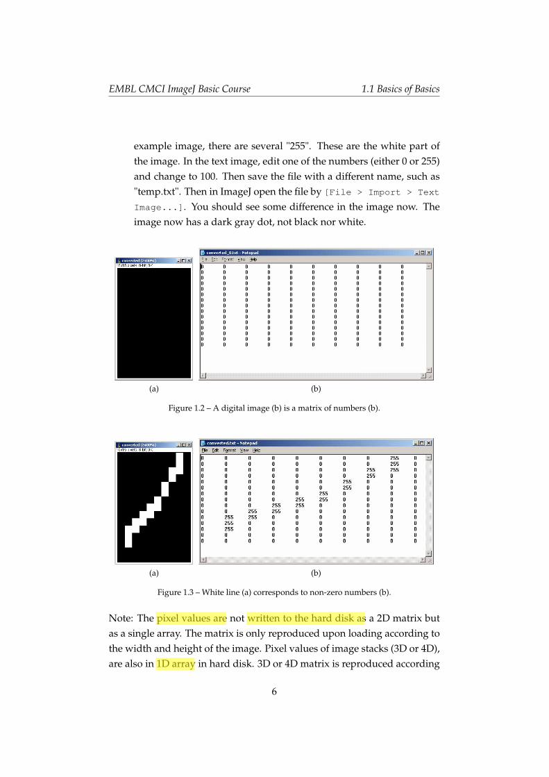
EMBL CMCI ImageJ Basic Course 1.1 Basics of Basics
example image, there are several "255". These are the white part ofthe image. In the text image, edit one of the numbers (either 0 or 255)and change to 100. Then save the file with a different name, such as"temp.txt". Then in ImageJ open the file by [File > Import > Text
Image...]. You should see some difference in the image now. Theimage now has a dark gray dot, not black nor white.
(a) (b)
Figure 1.2 – A digital image (b) is a matrix of numbers (b).
(a) (b)
Figure 1.3 – White line (a) corresponds to non-zero numbers (b).
Note: The pixel values are not written to the hard disk as a 2D matrix butas a single array. The matrix is only reproduced upon loading according tothe width and height of the image. Pixel values of image stacks (3D or 4D),are also in 1D array in hard disk. 3D or 4D matrix is reproduced according
6
EMBL CMCI ImageJ Basic Course 1.1 Basics of Basics
to additional information such as slice and channel number. Such informa-tion is written in the "header" region of the file, which precedes the "data"region of the file where the 1D array of pixel array is contained. The headerstructure depends on the file format, many such formats exist (the mostcommon are TIFF or BMP, we will see more in "file formats and header"section).
1.1.2 Image Bit-Depth
Image file has a defined bit depth. You might have already heard termslike "8-bit" or "16-bit" and these are the bit depth. 8-bit means that the gray-scale of the image has 28 = 256 steps: in other words, the grayness betweenblack and white is divided into 256 steps. In the same way 16-bit translatesto 216 = 65536 steps, hence for 16-bit images one can assign gray-level topixels in a much more precise way; in other words "grayness resolution" ishigher.
Microscope images are generated mostly by CCD camera (orsomething similar). CCD chip has a matrix of sensors. Eachsensor receives photons and converts the number of photonsto a value for a pixel at the corresponding position within theimage. Larger bit-depth enables more detailed conversion ofsignal intensity (infinite steps) to pixel values (limited steps).
Why do we use "2n"? This is because computers code the information withbinary numbers. In binary the elementary units are called bits and thereonly possible values are 0 and 1 (in the decimal system these units are calleddigits and can take values from 0 to 9). Coding values with 8-bit means forexample that this value is represented as a 8 bit number, something like"00001010" ( = 10 in decimal). Then the minimum value is = "00000000"("0" in decimal) and the maximum is 11111111 ("255" in decimal). 8-bit im-age allows 256 scales for the grayness (using calculator application in yourcomputer, you could easily convert binary number into normal decimalsand vice versa). In case of 16-bit image, the scale is 216 so there are 65536steps.
7

EMBL CMCI ImageJ Basic Course 1.1 Basics of Basics
We must not forget that the nature is continuous. In conventional math-ematics (as you learn in school), a decimal point enables you to representinfinite steps between 0 and 1. But by digitizing the nature we lose the abil-ity to encode infinite steps such that 0.44 might be rounded to 0 and 0.56 to1. Thus, the bit-depth limits the resolution of the analog to digital conver-sion (AD conversion). Higher bit depth generally allows higher resolution.
ImageJ has a high-bit-depth format called signed 32-bit floating point im-age. In all above cases with 8-bit and 16-bit, the pixel value is representedin integer but floating-point type enables decimal points (real number) forthe pixel value such as "15.445". Though 32-bit floating point image can beused for image calculation, many functions in ImageJ do not handle themproperly so cares should be taken when using this image format. If youwant to know more about the 32-bit format, read the following box (a bitcomplicated; you could just pass through)
32 bit FLOATING POINT images utilizes efficient use of the32 bits. Instead of using 32 bits to describe 4,294,967,296 integernumbers, 23 bits are allocated to a fraction, 8 bits to an expo-nent, and 1 bit to a sign, as follows:
V = (−1)S ∗ 1.F ∗ 2(E− 127),whereby:S = Sign, uses 1 bit and can have 2 possible valuesF = Fraction, uses 23 bits and can have 8,388,608 possible valuesE = Exponent, uses 8 bits and can have 256 possible values
Practically speaking, this allows for an almost infinite numberof tones between level "0" and "1", more than 8 million tonesbetween level "1" and "2" and 128 tones between level "65,534"and "65,535", much more in line with our human vision than a32 bit integer image. Because of the infinitesimally small num-bers that can be stored, the 32 bit floating point format allowsto store a virtually unlimited dynamic range. In other words,32 bit floating point images can store a virtually unlimited dy-namic range in a relatively compact way with more detail in the
8
EMBL CMCI ImageJ Basic Course 1.1 Basics of Basics
shadows than in the highlights and take up only twice the sizeof 16 bits per channel images, saving memory and processingpower. A higher accuracy format allows for smoother dynamicand tonal range compression.
(Quote from http://www.dpreview.com/learn/?/key=bits)
Guide Line for the Choice of Bit-Depth
In fluorescence microscopy, the choice of whether to use higher bit-depthformat depends on a balance among the intensity of excitation light, theemision signal intensity, the sensitivity of photon detector, quantum effi-ciency3 and the gain. If the signal is bright enough then there would goodS/N that you could simply use a lower bit depth but if the signal is toobright then you might need to use a higher bit depth just to avoid saturat-ing the bits. This balancing could also be controlled by changing the gainof the camera. In the end, the choice of bit depth depends on what typeof measurement you want to achieve. If you only need to determine theshape of the target object (“segmentation”), you might not need a higherbit depth image as you could try to adjust the imaging condition ratherthan increasing the file size of the image. On the other hand, if you are try-ing to measure protein density, a higher bit depth allows you to have moreprecise measurements so a larger bit-depth is recommended. A draw backis that it takes longer time for data transferring as the bit-depth becomeslarger. This may in turn limits the time resolution of image sequences. Thebalancing between imaging conditions and the type of analysis afterwardis very much coupled and should be thought well before your experiment.More details on this discussion could be found in microscopy textbook suchas Pawley (2006).
The choice of bit depth depends on deals with noise. Here is an explanationfrom Sébastien Tosi:
When minute details need to be preserved in both high and low
3Quantum effeciency is a measure of proportion of photons converted to electric im-pluse. For example, QE of photographic film is ca. 10%, that of human eye is 20%. RecentCCD allows 80%.
9
EMBL CMCI ImageJ Basic Course 1.1 Basics of Basics
intensity regions of a sample a large bit-depth is necessary toensure a good image quality. Indeed for low bit-depth if the sig-nal level is adjusted to avoid saturation in the brightest regionsthere is a high risk to end up coding the signal of the faintest re-gions over only very few bits, which has a very detrimental ef-fect on the image quality. A large bit depth is hence necessary toprovide a fine slicing of the intensity range while provisioninga sufficient headroom to avoid saturation and as such alwaysthe safest option.
It can be mathematically derived that quantizing a continuoussignal to a finite number of levels induces an Additive White(un-correlated) noise commonly called “quantization noise”. Thelevel of this noise source is conditioned by the number of levelsthat are allowed (over the effective range of the signal). De-pending on the image intrinsic noise (shot noise at a given pho-ton regime) and the noises coming from the detector and theamplifier electronics this noise can eventually be neglected. Oneshould always make sure that this noise source can be neglectedto avoid trashing valuable (available) information.
(personal communication, Sébastien Tosi)
1.1.3 Converting the bit-depth of an image
In many occasions, you might want to decrease the bit-depth of image sim-ply to reduce the file size (16-bit file becomes half the file size when it is con-verted to 8-bit), or you might need to use certain algorithm that is availableonly with 8-bit images (there are many such cases), or so on. In any case,this will be a good experience for you to see the limitation of bit-depth.
Here, we focus on the conversion of a 16-bit image to an 8-bit image tostudy its effect and associated possible errors.
Exercise 1.1.3-1
Let’s first open a 16-bit image from the sample. If you have the courseplugin installed, choose the menu item [EMBL > Samples > m51.tif].Otherwise, if you have sample images saved in your local machine,
10
EMBL CMCI ImageJ Basic Course 1.1 Basics of Basics
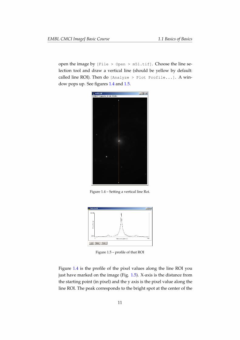
open the image by [File > Open > m51.tif]. Choose the line se-lection tool and draw a vertical line (should be yellow by default:called line ROI). Then do [Analyze > Plot Profile...]. A win-dow pops up. See figures 1.4 and 1.5.
Figure 1.4 – Setting a vertical line Roi.
Figure 1.5 – profile of that ROI
Figure 1.4 is the profile of the pixel values along the line ROI youjust have marked on the image (Fig. 1.5). X-axis is the distance fromthe starting point (in pixel) and the y axis is the pixel value along theline ROI. The peak corresponds to the bright spot at the center of the
11
EMBL CMCI ImageJ Basic Course 1.1 Basics of Basics
image.
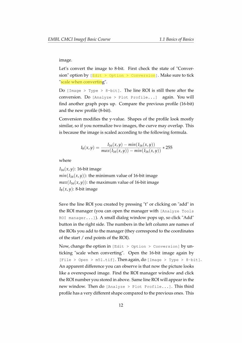
Let’s convert the image to 8-bit. First check the state of "Conver-sion" option by [Edit > Option > Conversion]. Make sure to tick"scale when converting".
Do [Image > Type > 8-bit]. The line ROI is still there after theconversion. Do [Analyze > Plot Profile...] again. You willfind another graph pops up. Compare the previous profile (16-bit)and the new profile (8-bit).
Conversion modifies the y-value. Shapes of the profile look mostlysimilar, so if you normalize two images, the curve may overlap. Thisis because the image is scaled according to the following formula.
I8(x, y) =I16(x, y)−min(I16(x, y))
max(I16(x, y))−min(I16(x, y))∗ 255
where
I16(x, y): 16-bit imagemin(I16(x, y)): the minimum value of 16-bit imagemax(I16(x, y)): the maximum value of 16-bit imageI8(x, y): 8-bit image
Save the line ROI you created by pressing "t" or clicking on "add" inthe ROI manager (you can open the manager with [Analyze Tools
ROI manager...]). A small dialog window pops up, so click "Add"button in the right side. The numbers in the left column are names ofthe ROIs you add to the manager (they correspond to the coordinatesof the start / end points of the ROI).
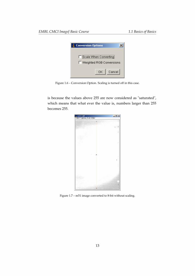
Now, change the option in [Edit > Option > Conversion] by un-ticking "scale when converting". Open the 16-bit image again by[File > Open > m51.tif]. Then again, do [Image > Type > 8-bit].An apparent difference you can observe is that now the picture lookslike a overexposed image. Find the ROI manager window and clickthe ROI number you stored in above. Same line ROI will appear in thenew window. Then do [Analyze > Plot Profile...]. This thirdprofile has a very different shape compared to the previous ones. This
12
EMBL CMCI ImageJ Basic Course 1.1 Basics of Basics
Figure 1.6 – Conversion Option. Scaling is turned off in this case.
is because the values above 255 are now considered as "saturated",which means that what ever the value is, numbers larger than 255becomes 255.
Figure 1.7 – m51 image converted to 8-bit without scaling.
13
EMBL CMCI ImageJ Basic Course 1.1 Basics of Basics
(a) (b)
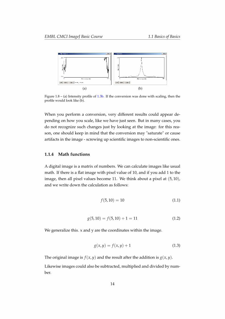
Figure 1.8 – (a) Intensity profile of 1.3b. If the conversion was done with scaling, then theprofile would look like (b).
When you perform a conversion, very different results could appear de-pending on how you scale, like we have just seen. But in many cases, youdo not recognize such changes just by looking at the image: for this rea-son, one should keep in mind that the conversion may "saturate" or causeartifacts in the image - screwing up scientific images to non-scientific ones.
1.1.4 Math functions
A digital image is a matrix of numbers. We can calculate images like usualmath. If there is a flat image with pixel value of 10, and if you add 1 to theimage, then all pixel values become 11. We think about a pixel at (5, 10),and we write down the calculation as follows:
f (5, 10) = 10 (1.1)
g(5, 10) = f (5, 10) + 1 = 11 (1.2)
We generalize this. x and y are the coordinates within the image.
g(x, y) = f (x, y) + 1 (1.3)
The original image is f (x, y) and the result after the addition is g(x, y).
Likewise images could also be subtracted, multiplied and divided by num-ber.
14
EMBL CMCI ImageJ Basic Course 1.1 Basics of Basics
Exercise 1.1.4-1
Simple math using 8-bit image: Prepare a new image following theinitial part of the exercise 1.1.1. Now, bring the mouse pointer overthe image and check the "value" that appears in the status bar in theImageJ window4. All pixel values in the image should be"value = 0"."x=. . . , y=. . . " in the status bar.
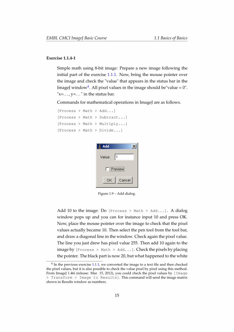
Commands for mathematical operations in ImageJ are as follows.
[Process > Math > Add...]
[Process > Math > Subtract...]
[Process > Math > Multiply...]
[Process > Math > Divide...]
Figure 1.9 – Add dialog.
Add 10 to the image: Do [Process > Math > Add...]. A dialogwindow pops up and you can for instance input 10 and press OK.Now, place the mouse pointer over the image to check that the pixelvalues actually became 10. Then select the pen tool from the tool bar,and draw a diagonal line in the window. Check again the pixel value.The line you just drew has pixel value 255. Then add 10 again to theimage by [Process > Math > Add...]. Check the pixels by placingthe pointer. The black part is now 20, but what happened to the white
4 In the previous exercise 1.1.1, we converted the image to a text file and then checkedthe pixel values, but it is also possible to check the value pixel by pixel using this method.From ImageJ 1.46i (release: Mar. 15, 2012), you could check the pixel values by [Image> Transform > Image to Results]. This command will send the image matrixshown in Results window as numbers.
15
EMBL CMCI ImageJ Basic Course 1.1 Basics of Basics
line?
Since the image bit-depth is 8, the available number is only between 0and 255. When you add 10 to a pixel with its value 255, the calculationreturns 255 because the number "265" does not exist in 8-bit world. Asimilar limitation applies to other mathematical operations too. If youmultiply a pixel value 100 by 3, the answer in normal mathematics is300. But in 8-bit world, that pixel becomes 255.
How about division? Close the currently working test image, andprepare a new image as you did in 1.1.1. Zoom up the image, andadd 100 ([Process > Math > Add...]; you should see the imageturns to gray from black). Check pixel values by placing the pointerabove the image. Now, Divide the image by 3 ([Process > Math >
Divide...]). Check the result by placing the mouse over the image.The pixel value is now 33. Since there is no decimal placeholder in 8-bit, the division returns the rounded value of (100 / 3 = 33). One couldalso divide image by any real number, such as 3.1415. The answer willbe in integer in all cases in 8-bit and 16-bit. In case of floating point32-bit image, the calculation results are different. We study this in thenext exercise.
Exercise 1.1.4-2
Simple Math on 32-bit Image: prepare a new 32-bit image (in the [New> Image..] dialog, select 32-bit from the "type" drop-down menu).Then add 100 to the image. Check that the image pixel values are all100. Then divide the image by 3. Check the answer. This time theresult has a decimal placeholder.
Bit-depth limitation of digital image is very important for you to know,in terms of quantitative measurements. Any measurement must be doneknowing the dynamic range of the detection system prior to the measure-ment. If you are trying to measure the amount of protein, and if some of the pixelsare saturated, then your measurement is invalid.
16
EMBL CMCI ImageJ Basic Course 1.1 Basics of Basics
1.1.5 Image Math
In the previous section we operated on a single image. Likewise, we canperform computations involving two images. For example, assuming twoimages f and g with same dimensions, and
f (5, 10) = 100 (1.4)
g(5, 10) = 50 (1.5)
. . . meaning that the pixel value at the position (5, 10) in the first image f is100 and in the second image g is 50, we can add these values and get a newimage h such that:
h(5, 10) = f (5, 10) + g(5, 10) = 100 + 50 = 150 (1.6)
This holds true for any pixel at position (x, y):
h(x, y) = f (x, y) + g(x, y) (1.7)
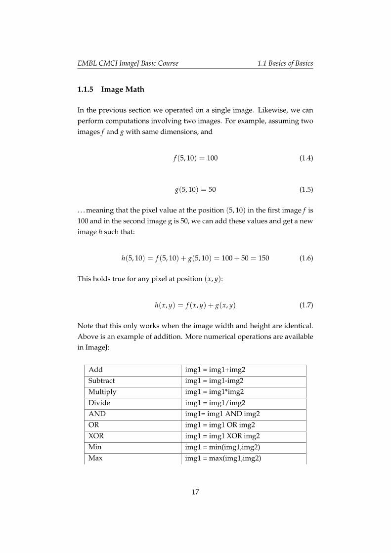
Note that this only works when the image width and height are identical.Above is an example of addition. More numerical operations are availablein ImageJ:
Add img1 = img1+img2
Subtract img1 = img1-img2
Multiply img1 = img1*img2
Divide img1 = img1/img2AND img1= img1 AND img2
OR img1 = img1 OR img2
XOR img1 = img1 XOR img2
Min img1 = min(img1,img2)Max img1 = max(img1,img2)
17
EMBL CMCI ImageJ Basic Course 1.1 Basics of Basics
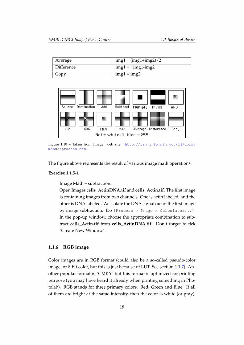
Average img1 = (img1+img2)/2
Difference img1 = |img1-img2|Copy img1 = img2
Figure 1.10 – Taken from ImageJ web site. http://rsb.info.nih.gov/ij/docs/menus/process.html
The figure above represents the result of various image math operations.
Exercise 1.1.5-1
Image Math – subtraction:Open Images cells_ActinDNA.tif and cells_Actin.tif. The first imageis containing images from two channels. One is actin labeled, and theother is DNA labeled. We isolate the DNA signal out of the first imageby image subtraction. Do [Process > Image > Calculator...].In the pop-up window, choose the appropriate combination to sub-tract cells_Actin.tif from cells_ActinDNA.tif. Don’t forget to tick"Create New Window".
1.1.6 RGB image
Color images are in RGB format (could also be a so-called pseudo-colorimage, or 8-bit color, but this is just because of LUT. See section 1.1.7). An-other popular format is "CMKY" but this format is optimized for printingpurpose (you may have heard it already when printing something in Pho-tolab). RGB stands for three primary colors. Red, Green and Blue. If allof them are bright at the same intensity, then the color is white (or gray).
18
EMBL CMCI ImageJ Basic Course 1.1 Basics of Basics
If only red is bright, then the color is red, and so on. A single RGB imagethus has three different channels. In other words, three layers of differentimages are overlaid in a single RGB image. Each channel (layer) has a bitdepth of 8-bit. So a single RGB image is 24-bit image. For this, the filesize of color pics becomes three times larger than a gray scale 8-bit image.Don’t save 16bit image in RGB format, since you lose a lot of information,for automatic conversion from 16 to 8 bit takes place.
Exercise 1.1.6-1
Working with RGB image:
(a) Open the image RGB_cell.tif by either [EMBL > Samples] or [File> Open]. Then split the color image to 3 different images [Image >
Color > Split Channels].
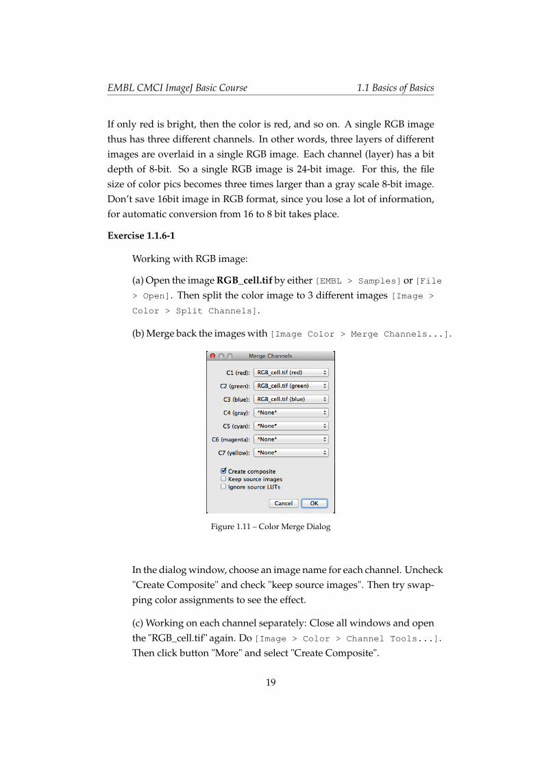
(b) Merge back the images with [Image Color > Merge Channels...].
Figure 1.11 – Color Merge Dialog
In the dialog window, choose an image name for each channel. Uncheck"Create Composite" and check "keep source images". Then try swap-ping color assignments to see the effect.
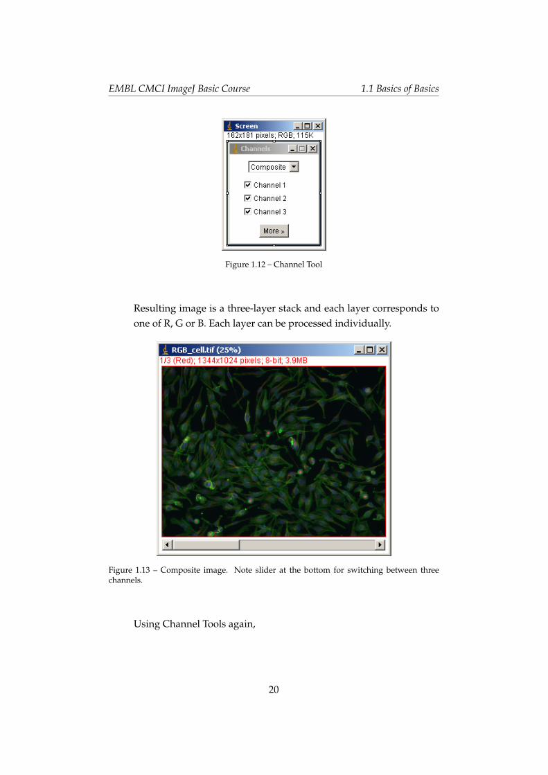
(c) Working on each channel separately: Close all windows and openthe "RGB_cell.tif" again. Do [Image > Color > Channel Tools...].Then click button "More" and select "Create Composite".
19
EMBL CMCI ImageJ Basic Course 1.1 Basics of Basics
Figure 1.12 – Channel Tool
Resulting image is a three-layer stack and each layer corresponds toone of R, G or B. Each layer can be processed individually.
Figure 1.13 – Composite image. Note slider at the bottom for switching between threechannels.
Using Channel Tools again,
20
EMBL CMCI ImageJ Basic Course 1.1 Basics of Basics
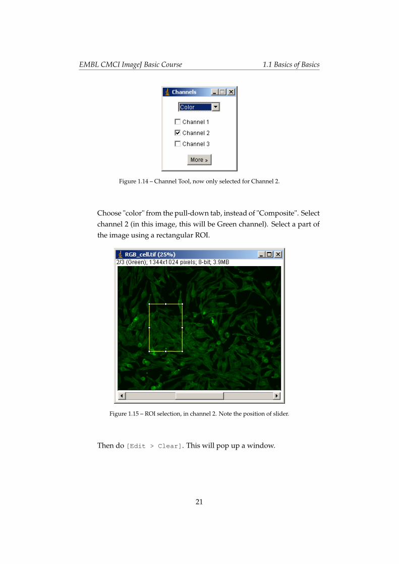
Figure 1.14 – Channel Tool, now only selected for Channel 2.
Choose "color" from the pull-down tab, instead of "Composite". Selectchannel 2 (in this image, this will be Green channel). Select a part ofthe image using a rectangular ROI.
Figure 1.15 – ROI selection, in channel 2. Note the position of slider.
Then do [Edit > Clear]. This will pop up a window.
21
EMBL CMCI ImageJ Basic Course 1.1 Basics of Basics
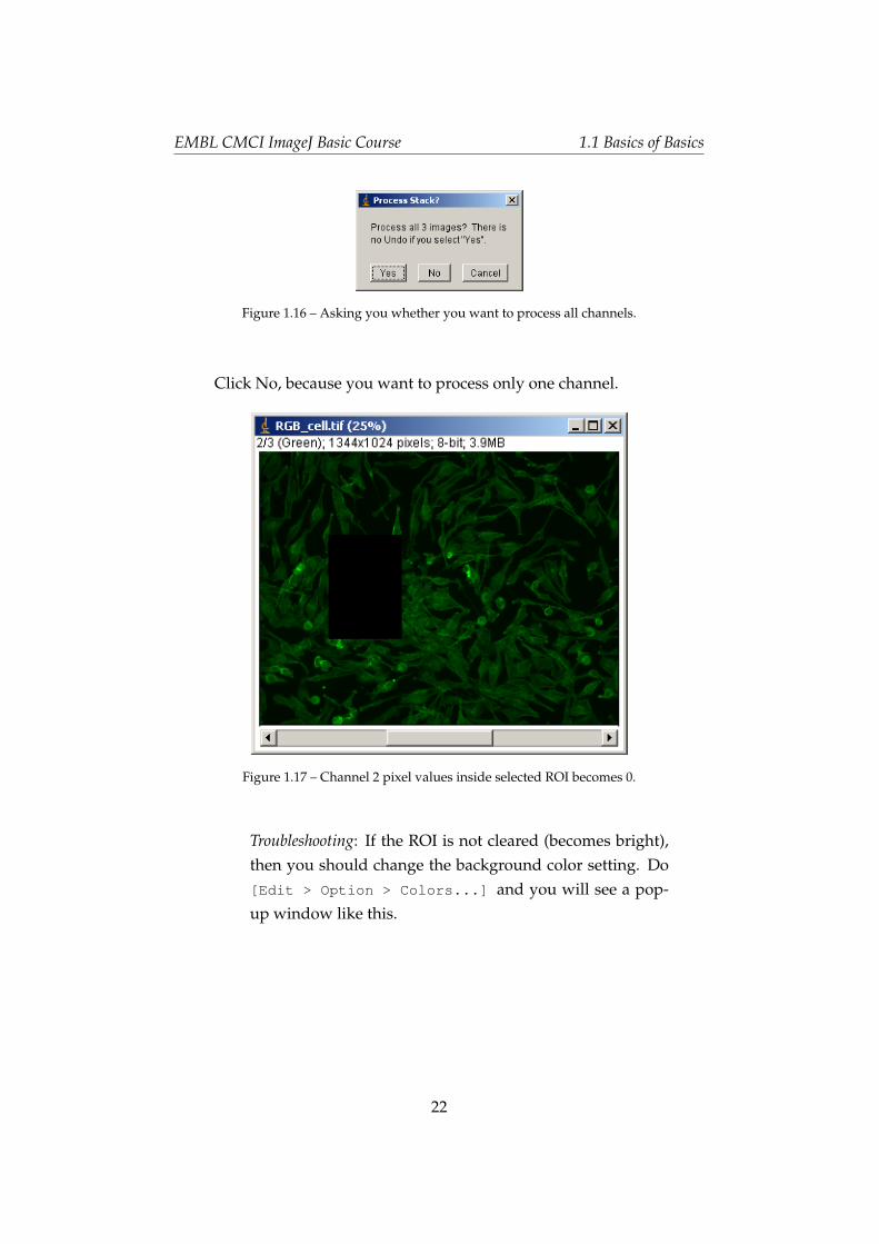
Figure 1.16 – Asking you whether you want to process all channels.
Click No, because you want to process only one channel.
Figure 1.17 – Channel 2 pixel values inside selected ROI becomes 0.
Troubleshooting: If the ROI is not cleared (becomes bright),then you should change the background color setting. Do[Edit > Option > Colors...] and you will see a pop-up window like this.
22
EMBL CMCI ImageJ Basic Course 1.1 Basics of Basics
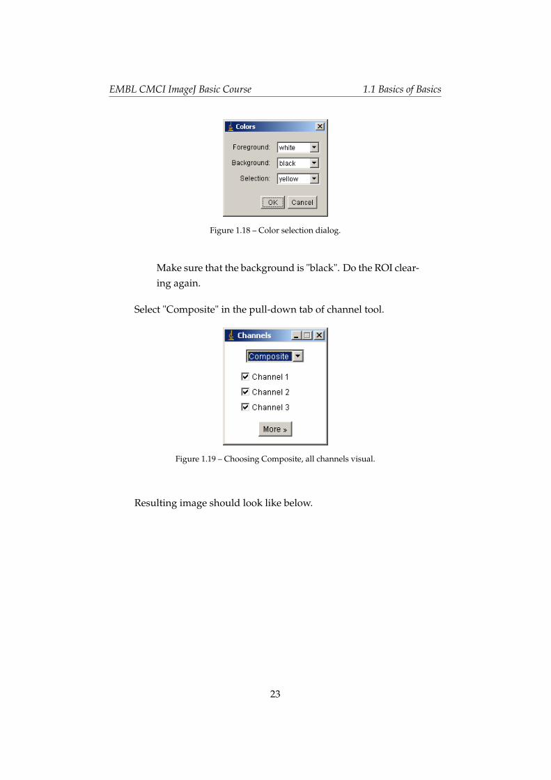
Figure 1.18 – Color selection dialog.
Make sure that the background is "black". Do the ROI clear-ing again.
Select "Composite" in the pull-down tab of channel tool.
Figure 1.19 – Choosing Composite, all channels visual.
Resulting image should look like below.
23
EMBL CMCI ImageJ Basic Course 1.1 Basics of Basics
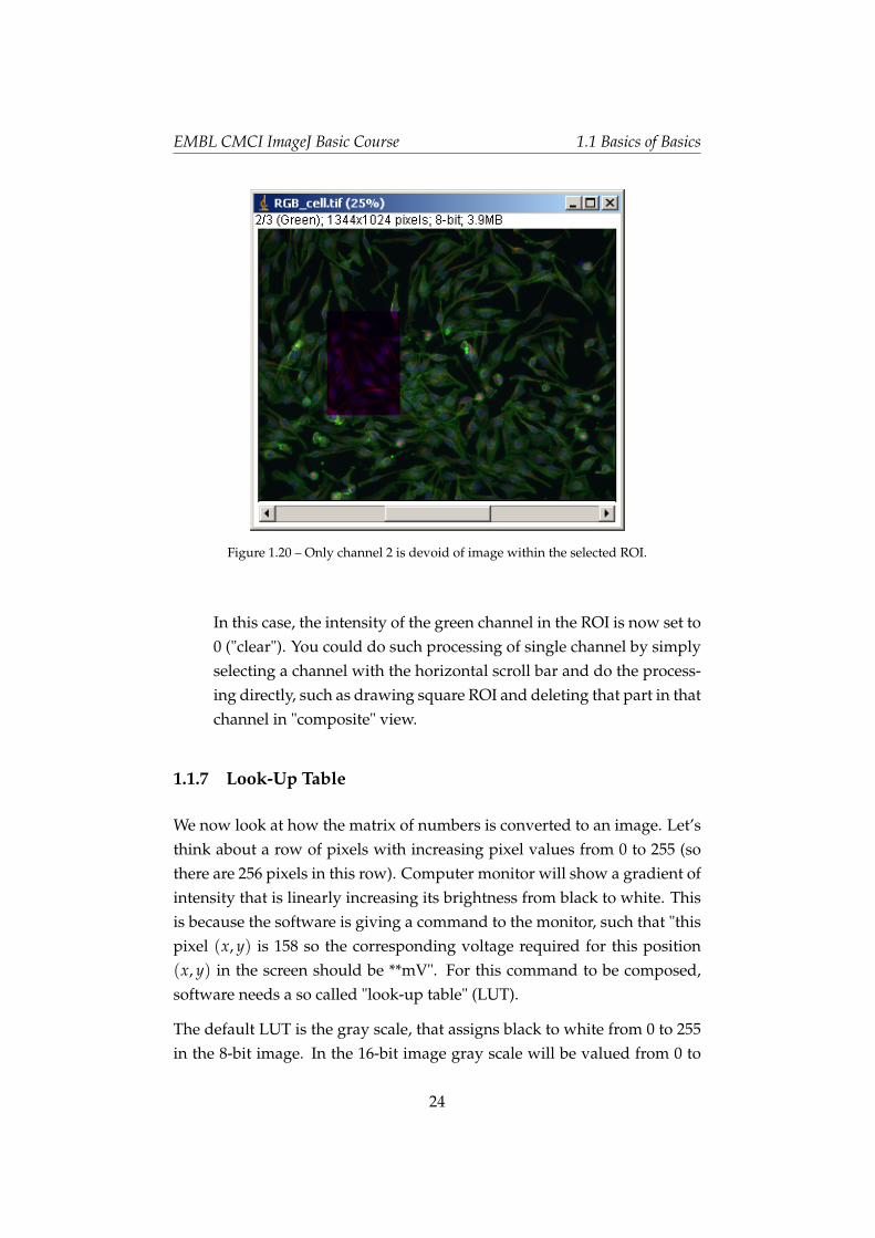
Figure 1.20 – Only channel 2 is devoid of image within the selected ROI.
In this case, the intensity of the green channel in the ROI is now set to0 ("clear"). You could do such processing of single channel by simplyselecting a channel with the horizontal scroll bar and do the process-ing directly, such as drawing square ROI and deleting that part in thatchannel in "composite" view.
1.1.7 Look-Up Table
We now look at how the matrix of numbers is converted to an image. Let’sthink about a row of pixels with increasing pixel values from 0 to 255 (sothere are 256 pixels in this row). Computer monitor will show a gradient ofintensity that is linearly increasing its brightness from black to white. Thisis because the software is giving a command to the monitor, such that "thispixel (x, y) is 158 so the corresponding voltage required for this position(x, y) in the screen should be **mV". For this command to be composed,software needs a so called "look-up table" (LUT).
The default LUT is the gray scale, that assigns black to white from 0 to 255in the 8-bit image. In the 16-bit image gray scale will be valued from 0 to
24
EMBL CMCI ImageJ Basic Course 1.1 Basics of Basics
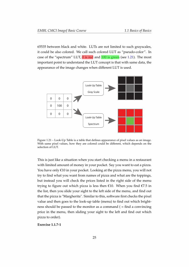
65535 between black and white. LUTs are not limited to such grayscales,it could be also colored. We call such colored LUT as “pseudo-color”. Incase of the “spectrum” LUT, 0 is red and 100 is green (see 1.21). The mostimportant point to understand the LUT concept is that with same data, theappearance of the image changes when different LUT is used.
Look-Up Table
Gray Scale
100
0 0 0
0 0
0 0 0Look-Up Table
Spectrum
Figure 1.21 – Look-Up Table is a table that defines appearance of pixel values as an image.With same pixel values, how they are colored could be different, which depends on theselection of LUT.
This is just like a situation when you start checking a menu in a restaurantwith limited amount of money in your pocket. Say you want to eat a pizza.You have only €10 in your pocket. Looking at the pizza menu, you will nottry to find what you want from names of pizza and what are the toppings,but instead you will check the prices listed in the right side of the menutrying to figure out which pizza is less then €10. When you find €7.5 inthe list, then you slide your sight to the left side of the menu, and find outthat the pizza is "Margherita". Similar to this, software first checks the pixelvalue and then goes to the look-up table (menu) to find out which bright-ness should be passed to the monitor as a command ( = find a convincingprice in the menu, then sliding your sight to the left and find out whichpizza to order).
Exercise 1.1.7-1
25
EMBL CMCI ImageJ Basic Course 1.1 Basics of Basics
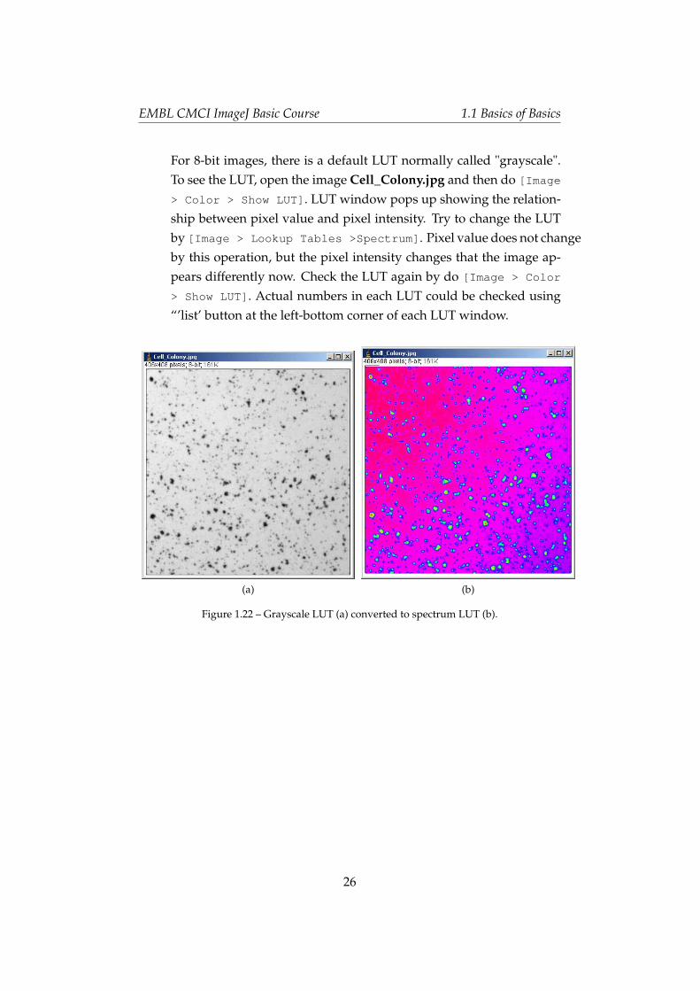
For 8-bit images, there is a default LUT normally called "grayscale".To see the LUT, open the image Cell_Colony.jpg and then do [Image
> Color > Show LUT]. LUT window pops up showing the relation-ship between pixel value and pixel intensity. Try to change the LUTby [Image > Lookup Tables >Spectrum]. Pixel value does not changeby this operation, but the pixel intensity changes that the image ap-pears differently now. Check the LUT again by do [Image > Color
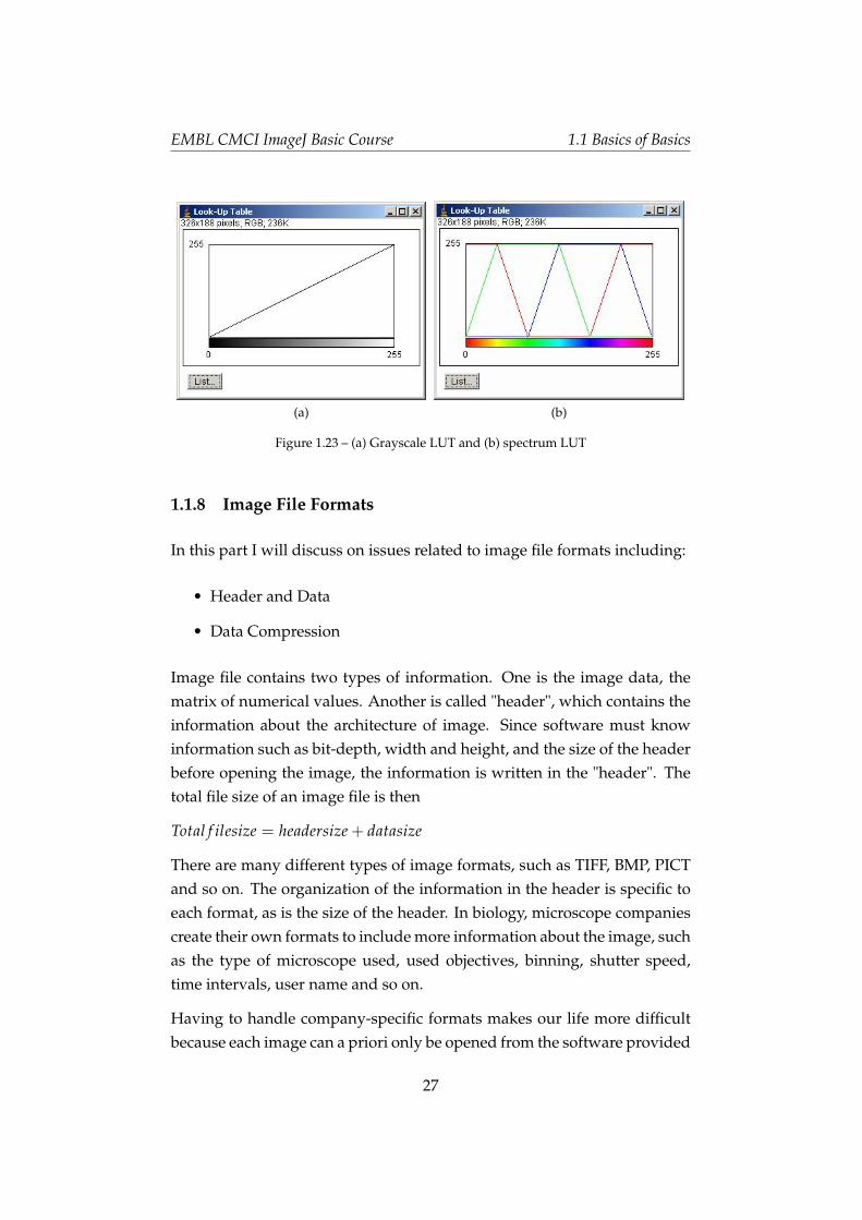
> Show LUT]. Actual numbers in each LUT could be checked using“’list’ button at the left-bottom corner of each LUT window.
(a) (b)
Figure 1.22 – Grayscale LUT (a) converted to spectrum LUT (b).
26
EMBL CMCI ImageJ Basic Course 1.1 Basics of Basics
(a) (b)
Figure 1.23 – (a) Grayscale LUT and (b) spectrum LUT
1.1.8 Image File Formats
In this part I will discuss on issues related to image file formats including:
• Header and Data
• Data Compression
Image file contains two types of information. One is the image data, thematrix of numerical values. Another is called "header", which contains theinformation about the architecture of image. Since software must knowinformation such as bit-depth, width and height, and the size of the headerbefore opening the image, the information is written in the "header". Thetotal file size of an image file is then
Total f ilesize = headersize + datasize
There are many different types of image formats, such as TIFF, BMP, PICTand so on. The organization of the information in the header is specific toeach format, as is the size of the header. In biology, microscope companiescreate their own formats to include more information about the image, suchas the type of microscope used, used objectives, binning, shutter speed,time intervals, user name and so on.
Having to handle company-specific formats makes our life more difficultbecause each image can a priori only be opened from the software provided
27
EMBL CMCI ImageJ Basic Course 1.1 Basics of Basics
by these companies. Fortunately there is an excellent ImageJ plugin whichenables importing specific image formats to ImageJ 5
You do not have to know all the details about the architecture of variousimage formats (thanks to the bioformats plugin), but it is important for youto know that the difference resides mainly in the header. The data part isin most cases same, something like what we have seen already using textimage (for more details on header, refer to the appendix 1.6.1 ).
Exercise 1.1.8-1
Accessing the image properties
Open the example image wt1.tif. Do [Image > Show Info...]. Scale(pixels/inch) is listed in the information window, which was read outfrom the header of the image. Then do [Image > Properties], alsoshowing the scale.
Compression: Image file size become huge as the size of the image becomelarger. There are convenient ways to reduce image file size by data com-pression. When you take a snap shot using commercial digital camera orsmart phone, saved images are always compressed. But keep in your mind:
There are two types of compression formats: loss-less and lossy formats. Inloss-less formats, pixel values generated by CCD are preserved even afterthe compression is made. On the other hand in lossy formats, pixel valuesbecome different from the original measured values and cannot be restored.PNG is a popular loss-less compression format that does NOT alter theoriginal pixel values. With this format, compression of images are done byshrinking redundant parts: for example, instead of having 100 pixels of 0values as a block, you could replace that part by saying “here, there are100 pixels of zeros”. If you need to compress files, using PNG format ispreferred for scientific image data.
Other more popular compression formats are like JPEG and GIF. JPEG isofen used in commercial diginal cameras. In addition to the redundancyshrinking explained above, the compression procedure tries to mathemat-ically interpolate some parts of the image to ignore small details. These
5 LOCI Bioformat Plugin:http://www.loci.wisc.edu/ome/formats.html
28
EMBL CMCI ImageJ Basic Course 1.1 Basics of Basics
are lossy formats as the process of compression discards some part of data.This causes artifacts in the image and it could even be "manipulation" ofdata. For this reason, we better avoid using lossy formats for measure-ments as we cannot recover the original uncompressed image once theyare converted.
I recommend not to compress data except for sharing of data for visualiza-tion purpose. The PNG format does not lose the original pixel values butdue to the file format conversion, the header information associated withthe original will be lost and this often causes problem in retrieving impor-tant information about images such as scales and time stamps.
1.1.9 Multidimensional data
In this section, we study the following topics.
• Image stacks
• Editing Stacks
• 4D stacks
• Hyperstacks
Multidimensional data, in which we define here as a set of image data withdimensions more than x and y. Multidimensional data have intrinsic lim-itation in displaying them on two dimensional screen. Efforts have beenmade to represent multidimensionality in various ways. One way is the“image stack”.
stacks
When you take time-lapse sequence or z-sections using a commercial mi-croscope system, the image files are generally saved in the company spe-cific file formats (e.g. .lsm or .lif files). Importing these images into ImageJcould simply be done using LOCI bioformats plugin.
29
EMBL CMCI ImageJ Basic Course 1.1 Basics of Basics
These image data appear as a series of images contained within a windowwith a scroll bar at the bottom. By scrolling, one could go through thethird dimension like a movie. This is the simplest form of multidimensionalrepresentation in 2D display.
In some cases, multidimensional data takes a form of multiple single imageframes with numbering such as
image0001.tifimage0002.tifimage0003.tif. . .
We can import such numbered files recursively and create a stack in ImageJ.
Exercise 1.1.9-1
We import multiple image files as an image stack. Download a zippedfile by [EMBL > Samples > Spindle-Frames.zip] 6. Unzip the fileby double clicking. Then [File > Import > Image Sequence...]
will open a dialog window and you must specify the first file of theimage series. Select sample sequence eg5_spindle_50000.tif. . . Thenanother dialog window pops up (Fig. 1.24).
6We do also have the stack directly downloadable, but we try to load numberd-tif imageshere.
30
EMBL CMCI ImageJ Basic Course 1.1 Basics of Basics
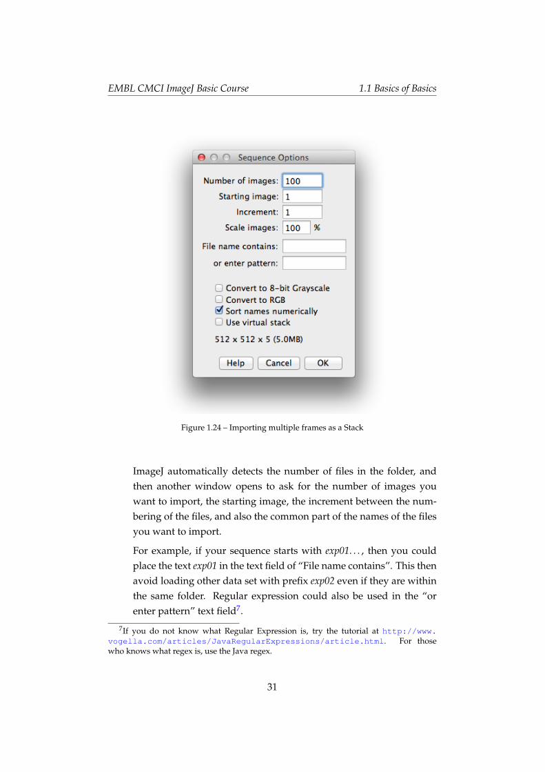
Figure 1.24 – Importing multiple frames as a Stack
ImageJ automatically detects the number of files in the folder, andthen another window opens to ask for the number of images youwant to import, the starting image, the increment between the num-bering of the files, and also the common part of the names of the filesyou want to import.
For example, if your sequence starts with exp01. . . , then you couldplace the text exp01 in the text field of “File name contains”. This thenavoid loading other data set with prefix exp02 even if they are withinthe same folder. Regular expression could also be used in the “orenter pattern” text field7.
7If you do not know what Regular Expression is, try the tutorial at http://www.vogella.com/articles/JavaRegularExpressions/article.html. For thosewho knows what regex is, use the Java regex.
31
EMBL CMCI ImageJ Basic Course 1.1 Basics of Basics
There are other options such as scaling and conversion of the imagebit depth, but these operations could be done afterward. The im-ported image sequence is within one window, or a stack.
A stack could be saved as a single file. File extension is typically ".tif",which is same as the single frame file. The file header will contain theinformation on the number of frames that the image contains. Thisnumber will be automatically detected when the stack is opened nexttime, so that the stack can be correctly reproduced.
Don’t close the stack, exercise continues.
Exercise 1.1.9-2
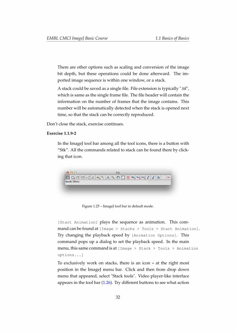
In the ImageJ tool bar among all the tool icons, there is a button with“Stk”. All the commands related to stack can be found there by click-ing that icon.
Figure 1.25 – ImageJ tool bar in default mode.
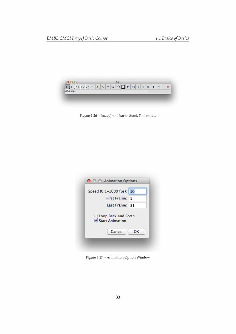
[Start Animation] plays the sequence as animation. This com-mand can be found at [Image > Stacks > Tools > Start Animation].Try changing the playback speed by [Animation Options]. Thiscommand pops up a dialog to set the playback speed. In the mainmenu, this same command is at [Image > Stack > Tools > Animation
options...]
To exclusively work on stacks, there is an icon » at the right mostposition in the ImageJ menu bar. Click and then from drop downmenu that appeared, select "Stack tools". Video player-like interfaceappears in the tool bar (1.26). Try different buttons to see what action
32
EMBL CMCI ImageJ Basic Course 1.1 Basics of Basics
Figure 1.26 – ImageJ tool bar in Stack Tool mode.
Figure 1.27 – Animation Option Window
33

EMBL CMCI ImageJ Basic Course 1.1 Basics of Basics
they perform.
Editing Stacks
In many occasions you might need to edit stacks such as
• Truncate a stack because you only need to analyze a part of the se-quence.
• For a presentation you need to combine two different stacks.
• Need to add a stack at the end of another stack.
• To make a combined stack by attaching each frame in a stack by aframe of another stack. Typically, you want to have two channels ofimage side-by side,
• You need only every second frame or slices to reduce the stack sizeby a half.
• To split two channel time series to individual time points withoutsplitting the channels.
• You need to insert a small inset within a stack.
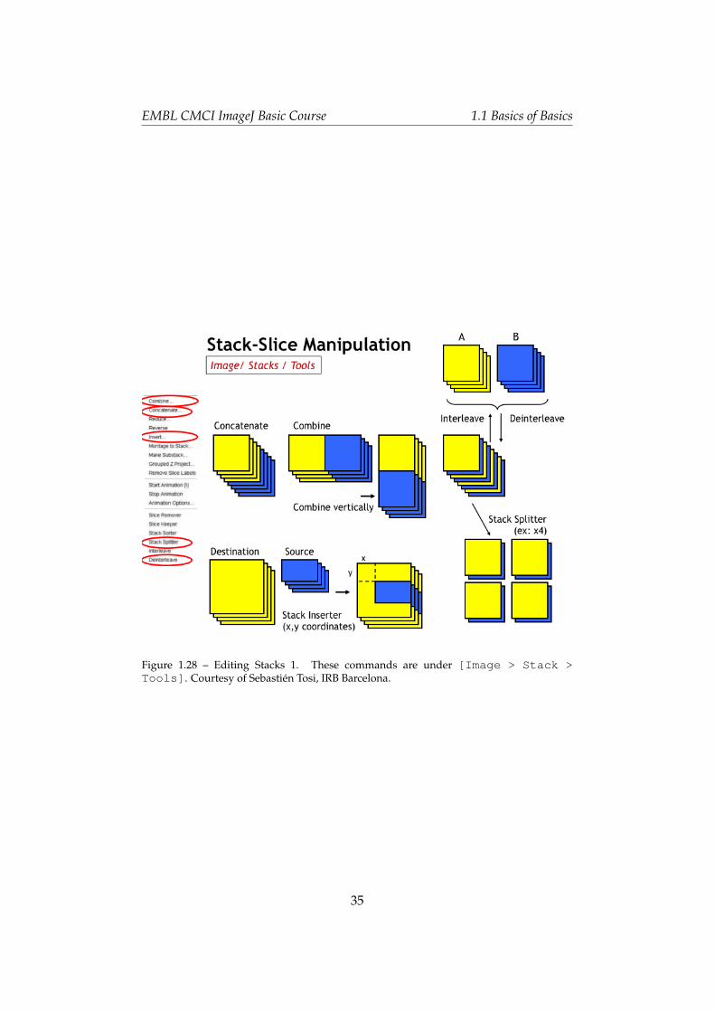
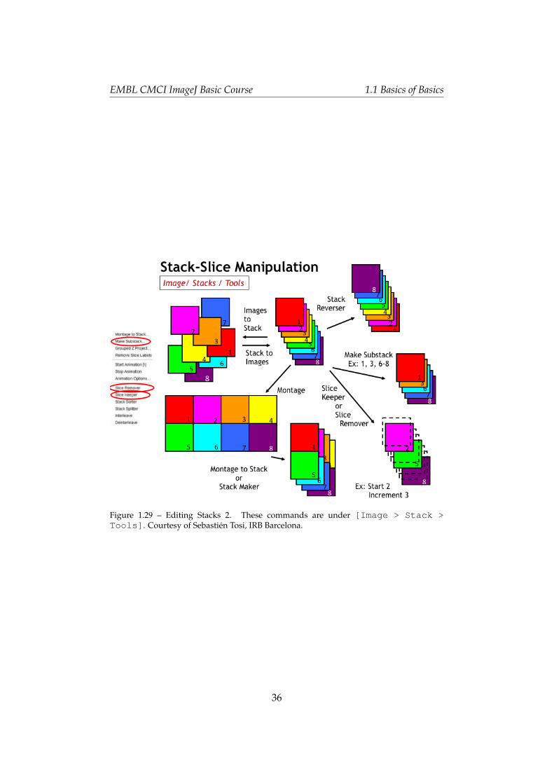
For such demands, tools for stack editing are available under the menutree [Image > Stack > Tools]. Figure 1.28 and figure 1.30 schematicallyshows what each of these commands does.
Exercise 1.1.9-3
Creating a MontageCreate a new image [File > New > Image...] with the followingproperties.
Name: could be any thing
•• Type: 8-bit
• Fill with: Black
• Width: 200
34
EMBL CMCI ImageJ Basic Course 1.1 Basics of Basics
Figure 1.28 – Editing Stacks 1. These commands are under [Image > Stack >Tools]. Courtesy of Sebastién Tosi, IRB Barcelona.
35
EMBL CMCI ImageJ Basic Course 1.1 Basics of Basics
Figure 1.29 – Editing Stacks 2. These commands are under [Image > Stack >Tools]. Courtesy of Sebastién Tosi, IRB Barcelona.
36
EMBL CMCI ImageJ Basic Course 1.1 Basics of Basics
• Height: 200
• Slices: 10
Then draw time stamps in each frame by Image > Stacks > Time
Stamper with the default properties but for the following:
X location: 50
•• Y location: 90
• Font Size: 36
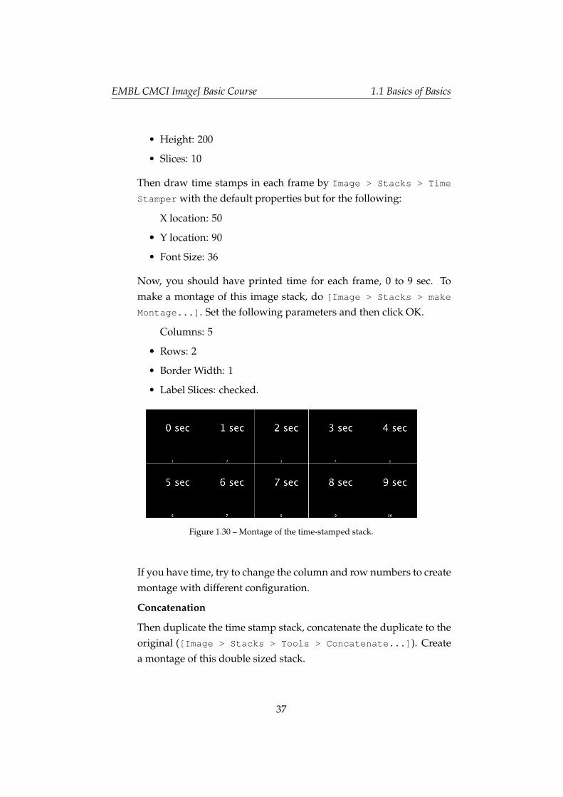
Now, you should have printed time for each frame, 0 to 9 sec. Tomake a montage of this image stack, do [Image > Stacks > make
Montage...]. Set the following parameters and then click OK.
Columns: 5
•• Rows: 2
• Border Width: 1
• Label Slices: checked.
Figure 1.30 – Montage of the time-stamped stack.
If you have time, try to change the column and row numbers to createmontage with different configuration.
Concatenation
Then duplicate the time stamp stack, concatenate the duplicate to theoriginal ([Image > Stacks > Tools > Concatenate...]). Createa montage of this double sized stack.
37
EMBL CMCI ImageJ Basic Course 1.1 Basics of Basics
4D stacks
A time-lapse sequences (we could call it “2DT stack” or xyt stack) or a Z-stack (we could call it “3D stack” or xyz stack) are relatively simple objectsbecause they are both made up of a series of two dimensional images. Morehighly dimensioned data are common these days. In many occasions wetake a time series of z-stacks maybe also with multiple channels. The or-der of two dimensional images within such multidimensional stacks thenbecomes an important issue. If we take an example of 3D time series, a pos-sible order of 2D images could start first with z-slices and then time series.In this case, the frame sequence will be something like this:
imgZ0-T1.tifimgZ1-T1.tifimgZ2-T1.tifimgZ0-T2.tifimgZ1-T2.tifimgZ2-T2.tifimgZ0-T3.tif. . .
The number after “Z” is the slice number and that after “T” is the file name.We often call this order “XYZT”. Alternatively, 2D images could be orderedwith time points first and then z-slices. In this case images will be stackedas:
imgZ0-T1.tifimgZ0-T2.tif. . .imgZ1-T1.tifimgZ1-T2.tif. . .imgZ2-T1.tifimgZ2-T2.tif. . .
We call this order “XYTZ”.
The order you will often find is the first one (XYZT) but in some cases you
38
EMBL CMCI ImageJ Basic Course 1.1 Basics of Basics
might also find the second one (XYTZ).
Stacks with more than 4D
If we have multiple channels, we could even have an order like “XYCZT”8
and so on. Since when viewed as a regular stack we can scroll only along asingle dimension the order of stack dimensions is fundamental as it effectsthe order in which the images will appear.
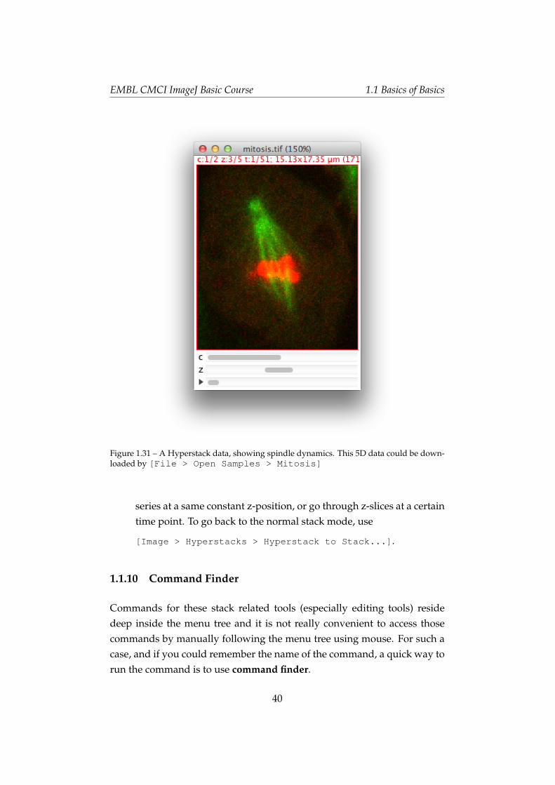
To avoid such complication with dimension ordering, there is an advancedformat of stack called Hyperstack. It could have up to three scroll bars at thebottom for channels (C), slices (Z) and time points (T) so one could easilyscroll through the dimension of your choice 1.31.
We will study more on the actual use of the image stacks in section 1.5.
Exercise 1.1.9-2
In this exercise, you will learn how to interact with image stacks (n Di-mensional images). Open sample image stack yeastDivision3DT.tif.This is a 3D time series stack. You can browse through the frames bymoving the scroll bar at the bottom of the frame. Since this is a 3Dtime series, you will see that each time point is a sub-stack of imagesat different optical sections.
To view the stack in a more convenient way, you could convert thestack to a hyperstack by
[Image > Hyperstacks > Stack to Hyperstack...].9
In “Hyperstack” mode, two scroll bars appear at the bottom of thewindow. One is for scrolling through z slices and the other to select atime point (frame). Each scroll bar could be moved independently ofthe other dimension, so you could for example go through the time
8XYCZT is a typical order but many microscope companies and software do not followthis typical order.
9If this conversion does not work properly, the first thing you could check is if the settingof the image dimension is properly set. To check this, [Image > Properties...]and check if slice (z) number and frame number (time points) are set correctly. For thesample image we use in this exercise, z should be 8 and frames should be 46.
39
EMBL CMCI ImageJ Basic Course 1.1 Basics of Basics
Figure 1.31 – A Hyperstack data, showing spindle dynamics. This 5D data could be down-loaded by [File > Open Samples > Mitosis]
series at a same constant z-position, or go through z-slices at a certaintime point. To go back to the normal stack mode, use
[Image > Hyperstacks > Hyperstack to Stack...].
1.1.10 Command Finder
Commands for these stack related tools (especially editing tools) residedeep inside the menu tree and it is not really convenient to access thosecommands by manually following the menu tree using mouse. For such acase, and if you could remember the name of the command, a quick way torun the command is to use command finder.
40
EMBL CMCI ImageJ Basic Course 1.1 Basics of Basics
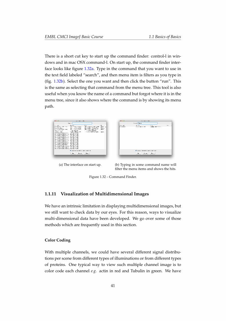
There is a short cut key to start up the command finder: control-l in win-dows and in mac OSX command-l. On start up, the command finder inter-face looks like figure 1.32a. Type in the command that you want to use inthe text field labeled “search”, and then menu item is filters as you type in(fig. 1.32b). Select the one you want and then click the button “run”. Thisis the same as selecting that command from the menu tree. This tool is alsouseful when you know the name of a command but forgot where it is in themenu tree, since it also shows where the command is by showing its menupath.
(a) The interface on start up. (b) Typing in some command name willfilter the menu items and shows the hits.
Figure 1.32 – Command Finder.
1.1.11 Visualization of Multidimensional Images
We have an intrinsic limitation in displaying multidimensional images, butwe still want to check data by our eyes. For this reason, ways to visualizemulti-dimensional data have been developed. We go over some of thosemethods which are frequently used in this section.
Color Coding
With multiple channels, we could have several different signal distribu-tions per scene from different types of illuminations or from different typesof proteins. One typical way to view such multiple channel image is tocolor code each channel e.g. actin in red and Tubulin in green. We have
41
EMBL CMCI ImageJ Basic Course 1.1 Basics of Basics
already scene such images in the RGB section (1.1.6).
The color coding is not limited to the dimensions in Channels, but also forslices (Z) and time points (T). By assigning a color that depends on the slicenumber or time points, the depth information within a Z-stack or a timepoint information with in a time lapse movie could be represented as aspecific color rather than by the position of that slice or frame within imagestack.
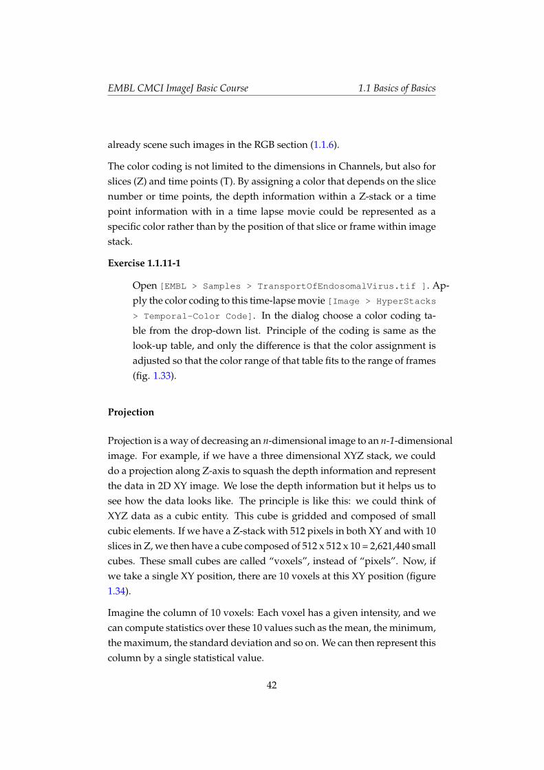
Exercise 1.1.11-1
Open [EMBL > Samples > TransportOfEndosomalVirus.tif ]. Ap-ply the color coding to this time-lapse movie [Image > HyperStacks
> Temporal-Color Code]. In the dialog choose a color coding ta-ble from the drop-down list. Principle of the coding is same as thelook-up table, and only the difference is that the color assignment isadjusted so that the color range of that table fits to the range of frames(fig. 1.33).
Projection
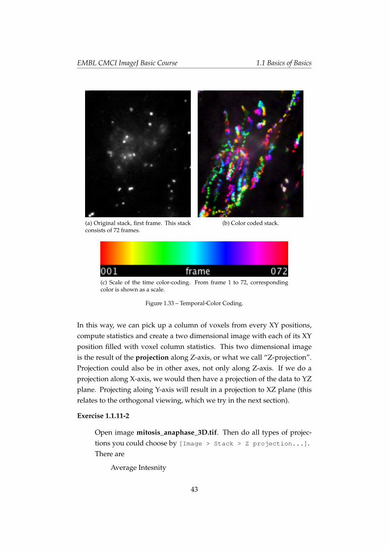
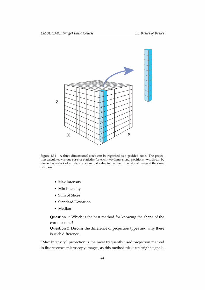
Projection is a way of decreasing an n-dimensional image to an n-1-dimensionalimage. For example, if we have a three dimensional XYZ stack, we coulddo a projection along Z-axis to squash the depth information and representthe data in 2D XY image. We lose the depth information but it helps us tosee how the data looks like. The principle is like this: we could think ofXYZ data as a cubic entity. This cube is gridded and composed of smallcubic elements. If we have a Z-stack with 512 pixels in both XY and with 10slices in Z, we then have a cube composed of 512 x 512 x 10 = 2,621,440 smallcubes. These small cubes are called “voxels”, instead of “pixels”. Now, ifwe take a single XY position, there are 10 voxels at this XY position (figure1.34).
Imagine the column of 10 voxels: Each voxel has a given intensity, and wecan compute statistics over these 10 values such as the mean, the minimum,the maximum, the standard deviation and so on. We can then represent thiscolumn by a single statistical value.
42
EMBL CMCI ImageJ Basic Course 1.1 Basics of Basics
(a) Original stack, first frame. This stackconsists of 72 frames.
(b) Color coded stack.
(c) Scale of the time color-coding. From frame 1 to 72, correspondingcolor is shown as a scale.
Figure 1.33 – Temporal-Color Coding.
In this way, we can pick up a column of voxels from every XY positions,compute statistics and create a two dimensional image with each of its XYposition filled with voxel column statistics. This two dimensional imageis the result of the projection along Z-axis, or what we call “Z-projection”.Projection could also be in other axes, not only along Z-axis. If we do aprojection along X-axis, we would then have a projection of the data to YZplane. Projecting aloing Y-axis will result in a projection to XZ plane (thisrelates to the orthogonal viewing, which we try in the next section).
Exercise 1.1.11-2
Open image mitosis_anaphase_3D.tif. Then do all types of projec-tions you could choose by [Image > Stack > Z projection...].There are
Average Intesnity
43
EMBL CMCI ImageJ Basic Course 1.1 Basics of Basics
z
yx
Figure 1.34 – A three dimensional stack can be regarded as a gridded cube. The projec-tion calculates various sorts of statistics for each two dimensional positions , which can beviewed as a stack of voxels, and store that value in the two dimensional image at the sameposition.
•• Max Intensity
• Min Intensity
• Sum of Slices
• Standard Deviation
• Median
Question 1: Which is the best method for knowing the shape of thechromosome?Question 2: Discuss the difference of projection types and why thereis such difference.
“Max Intensity” projection is the most frequently used projection methodin fluorescence microscopy images, as this method picks up bright signals.
44
EMBL CMCI ImageJ Basic Course 1.1 Basics of Basics
“sum of slices” method returns a 32bit image since results of addition couldpossibly exceed 8 bit or 16 bit range.
Note 1: If your data is a 3D time series hyper stack, there will be a smallcheck box in the projection dialog "All Time Points". If you check the box,projection will be done for each time point and the result will be a 2D timeseries of projections.
Note 2: The projection of a 2D time series can also be performed. Thoughtthe command name is “Z-Projection”, the principle of projection is identicalregardless of the projection axis.
Orthogonal Views
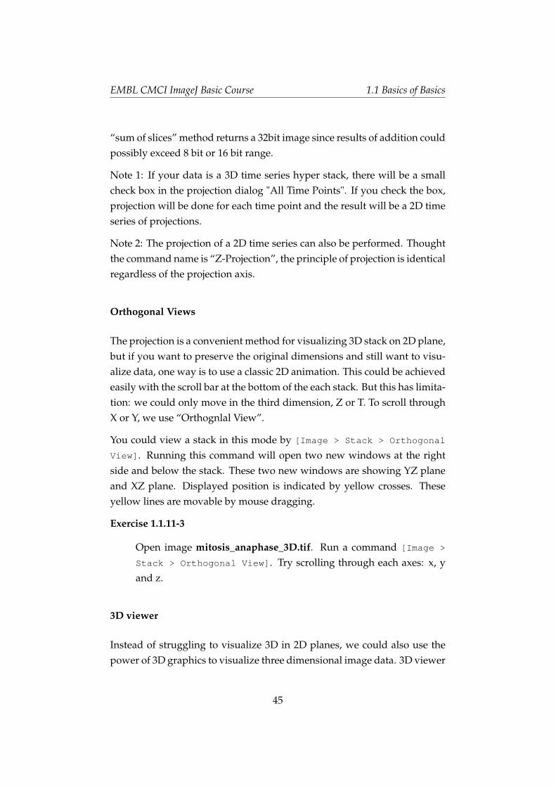
The projection is a convenient method for visualizing 3D stack on 2D plane,but if you want to preserve the original dimensions and still want to visu-alize data, one way is to use a classic 2D animation. This could be achievedeasily with the scroll bar at the bottom of the each stack. But this has limita-tion: we could only move in the third dimension, Z or T. To scroll throughX or Y, we use “Orthognlal View”.
You could view a stack in this mode by [Image > Stack > Orthogonal
View]. Running this command will open two new windows at the rightside and below the stack. These two new windows are showing YZ planeand XZ plane. Displayed position is indicated by yellow crosses. Theseyellow lines are movable by mouse dragging.
Exercise 1.1.11-3
Open image mitosis_anaphase_3D.tif. Run a command [Image >
Stack > Orthogonal View]. Try scrolling through each axes: x, yand z.
3D viewer
Instead of struggling to visualize 3D in 2D planes, we could also use thepower of 3D graphics to visualize three dimensional image data. 3D viewer
45
EMBL CMCI ImageJ Basic Course 1.1 Basics of Basics
(a) XY (b) YZ
(c) XZ
Figure 1.35 – Orthogonal View of a 3D stack.
is a plugin written by Benne Schimidt. It uses Java OpenGL (JOGL) to ren-der three dimensional data as click-and-rotatable object on your desktop.We could try to use the 3D viewer with the data we have been previouslydealing with.
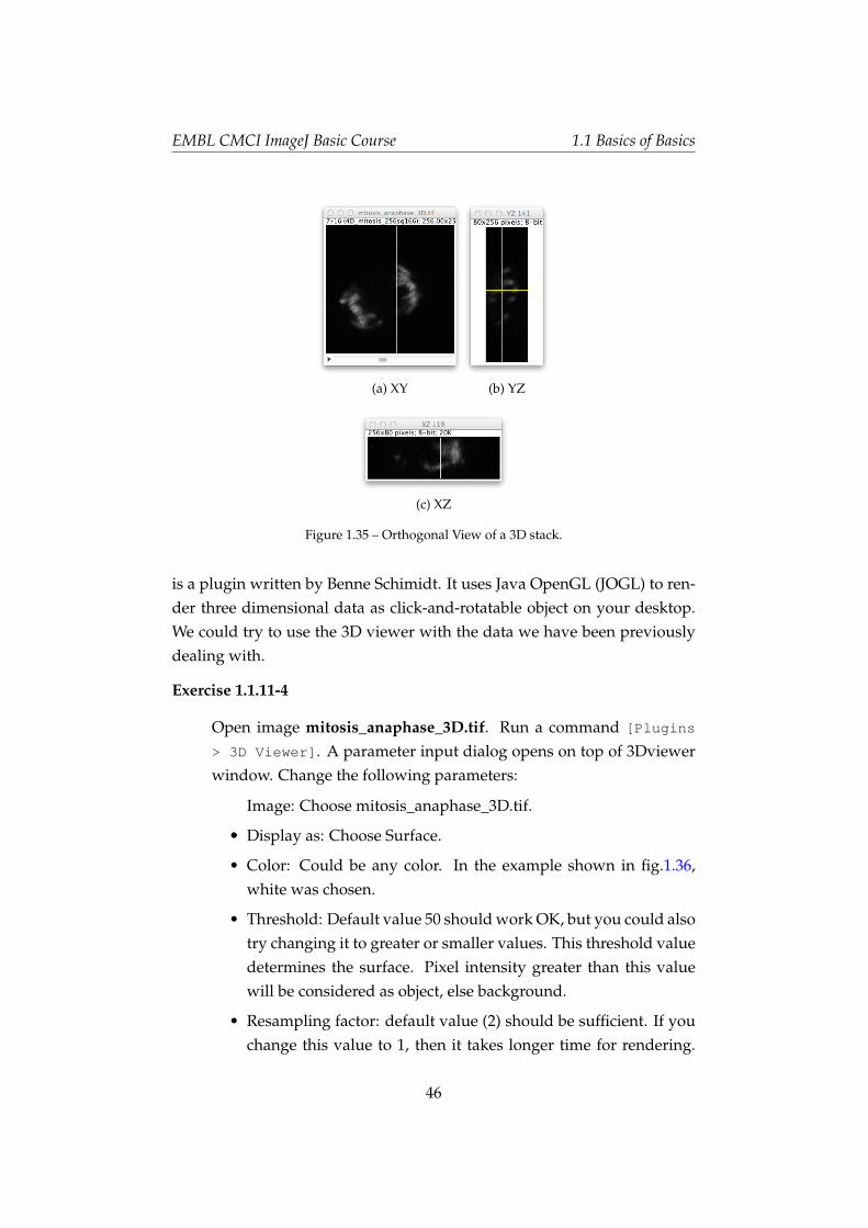
Exercise 1.1.11-4
Open image mitosis_anaphase_3D.tif. Run a command [Plugins
> 3D Viewer]. A parameter input dialog opens on top of 3Dviewerwindow. Change the following parameters:
Image: Choose mitosis_anaphase_3D.tif.
•• Display as: Choose Surface.
• Color: Could be any color. In the example shown in fig.1.36,white was chosen.
• Threshold: Default value 50 should work OK, but you could alsotry changing it to greater or smaller values. This threshold valuedetermines the surface. Pixel intensity greater than this valuewill be considered as object, else background.
• Resampling factor: default value (2) should be sufficient. If youchange this value to 1, then it takes longer time for rendering.
46
EMBL CMCI ImageJ Basic Course 1.1 Basics of Basics
In case of our example image which is small, difference in therendering time should be not really recognizable.
After setting these values, clicking “OK” will render the image in the3Dviewer window. Try to click and rotate the object.
(a) Parameter Input Dialog (b) Surface rendered 3D stack
Figure 1.36 – Surface rendering by 3DViewer.
More advanced usages are available such as visualizing two channels orshowing 3D time series as a time series of 3D graphics or saving movies.For such usages, consult the tutorial in the 3DViewer website (http://3dviewer.neurofly.de/).
1.1.12 Resampling images (Shrinking and Enlarging)
When you want to check the details of images, zooming is the best wayto focus on a specific region to observe details. Zooming is done by themagnification tool (icon of magnification glass) and this simply enlarges orshrinks the pixels.
Instead if you really need to increase the number of pixels per distance, wecall such processing as “Resampling” and we will examine this a bit in thissection.
By the way, if we just want to have larger image by adding some margin,
47
EMBL CMCI ImageJ Basic Course 1.1 Basics of Basics
we call this “resizing”, and the command for this resides in the menu treeunder [Image > Adjust > Canvas Size].
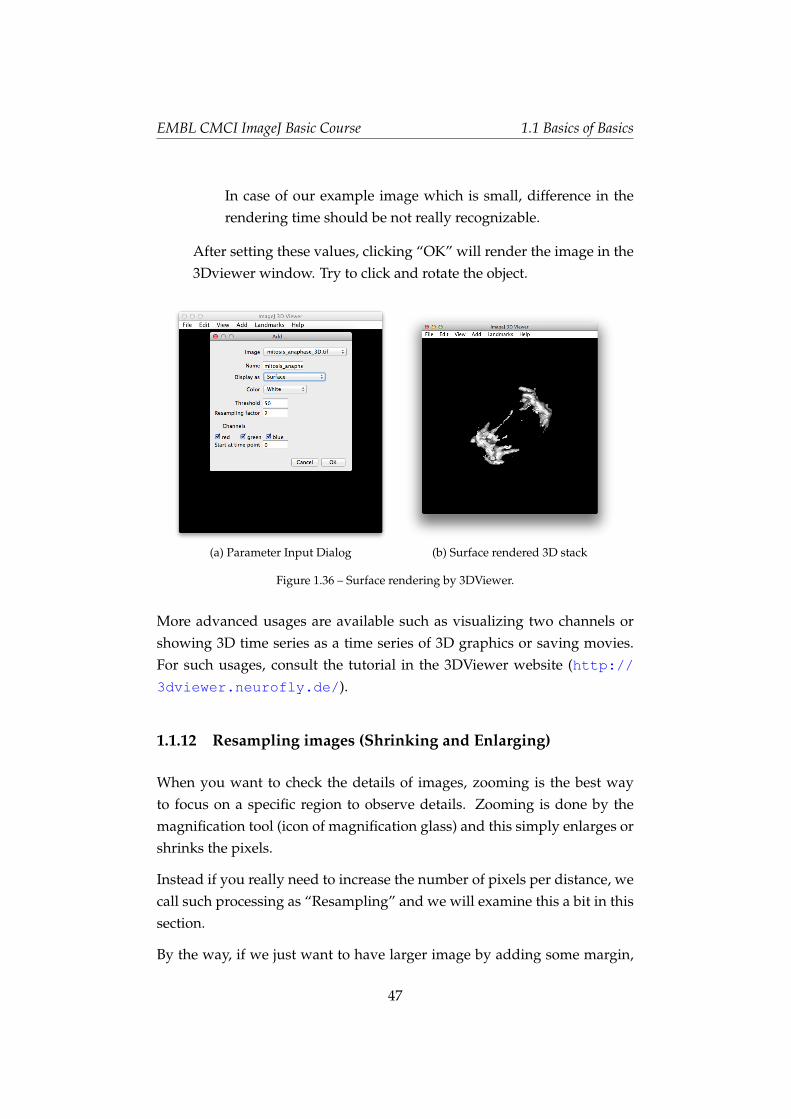
The resampling changes the original data. If we have an image of size 10pixels by 10 pixels and resample it to 200%, the image becomes 20 x 20. Ifwe resample it by 50%, then the image becomes 5 x 5. The resampling isa simple task that could be done by [Image > Adjust > Size...]. Thisis a simple operation but one must take care about how pixels will be pro-duced while enlarging and reduced while shrinking. If the enlarging issimply two times larger, we could imagine that each pixel will be copiedthree times to produce a block of four pixels to complete the task. The pixelvalues of the newly inserted pixels will then be identical to the source pixel.
But what happens if we want to enlarge the image by 150 %? To simplifythe situation, think about an image with 2 x 2 pixels. Then the resultingimage becomes 3 x 3. To understand the effect, do the following exercise.
Exercise 1.1.12-1
Open the example image 4pixelimage_sample.tif. The image is ultrasmall, so zoom it up to the maximum (as much as you can, you mustclick on or Ctrl - +). You now see four pixels in the window. Dupli-cate the image by [Image > Duplicate]. Magnify again. "Select all"by [Edit > Selection > Select All]. Then [Image > Adjust
> Size...]. In the dialog window, input the width 4 and height 4(corresponds to 200% enlargement). Tick "aspect ratio" and un-tick"Interpolation". Then click OK. Check the pixel values in original im-age, and the enlarged image.
Exercise 1.1.12-2
Do the similar resampling, but this time enlarge the image by 150%.Check the pixel values.
The resampling in the exercise was without interpolation – the check boxwas OFF. Interpolation is similar to the one dimensional interpolation wedo with graphs. In case of images, the gradient is also two dimensionalso the situation is a bit more complex. There are various methods for in-terpolating image. The interpolation method used in ImageJ is the bilinear
48
EMBL CMCI ImageJ Basic Course 1.1 Basics of Basics
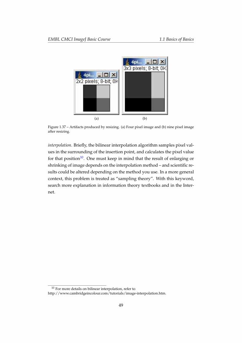
(a) (b)
Figure 1.37 – Artifacts produced by resizing. (a) Four pixel image and (b) nine pixel imageafter resizing.
interpolation. Briefly, the bilinear interpolation algorithm samples pixel val-ues in the surrounding of the insertion point, and calculates the pixel valuefor that position10. One must keep in mind that the result of enlarging orshrinking of image depends on the interpolation method – and scientific re-sults could be altered depending on the method you use. In a more generalcontext, this problem is treated as “sampling theory”. With this keyword,search more explanation in information theory textbooks and in the Inter-net.
10 For more details on bilinear interpolation, refer tohttp://www.cambridgeincolour.com/tutorials/image-interpolation.htm.
49

EMBL CMCI ImageJ Basic Course 1.1 Basics of Basics
1.1.13 ASSIGNMENTS
Assignment 1-1-1: Digital image = matrix of numbers
Edit a text image using any text editor. Be sure to insert space betweennumbers as separator. Save the text file and open it as an image in ImageJby importing text image function.
Assignments 1-1-2: bit depth
1. How many gray scale steps does a 12-bit image have?
2. Describe in text how a 1-bit image looks like.
Assignment 1-1-3: bit depth conversion
Use m51.tif (16-bit!) sample image to draw a plot profile, as we did inthe course. In the profile plot window, a "list" button is at the left-bottomcorner. Click the button. You will then see a new window containing acolumn of numbers. These numbers can be copy & pasted to spread sheetsoftware such as LibreOffice or MS Excel( or import the buffer to R). Youcould then plot the profile in those applications.
Compare original 16bit profile, 8-bit profiles with and without scaling byplotting three curves in a graph, and discuss the difference.
Assignments 1-1-4: Simple math on Images
1. Try subtracting certain values from the image you created in the As-signment 1-1-1 and check that the values cannot be less than 0.
2. Prepare an 8-bit image with pixel value 200. Divide the image by 3,and check the result.
3. Prepare a 16-bit image. In the [File > New > Image...] dialog,select 16-bit from the "type" drop-down menu. Try adding certainvalue to check the maximum pixel value.
4. Discuss why measurement of fluorescence intensity using digital im-age is invalid when some pixels are saturated.
50
EMBL CMCI ImageJ Basic Course 1.1 Basics of Basics
Assignments 1-1-5: LUT
Open "Cell_Colony.tif". Use LUT edit function and design your own LUTto highlight the black dots in Green and the background in Black. "LUT ed-itor" can be activated by [Images > Color > Edit LUT...]. Instructionfor the LUT editor is athttp://rsb.info.nih.gov/ij/plugins/lut-editor.html
You might be able to manage using it without reading the web instruction;just try!). LUT (.lut file) could also be edited using Excel.
Assignments 1-1-6: File size and image bit depth, image size
If there is an image with width = 100 pixels and height = 200 pixels, whatwould be the expected size of the image file in bytes? 1 byte = 8-bit.
Create a new image with the dimension as above, and save the image in"bitmap (.bmp)" format and check the file size. Is it same as you expected,or different? Save the same image in text file format and check the file sizeagain.
Assignment 1-1-7 Resizing
1. Enlarge the sample image 4pixelimage_sample.tif by 150% while the"Interpolation" check box in the size adjustment window is ON. Studythe pixel values before and after the enlargement. What happened?Describe the result.
2. Change "canvas size" by [Image > Adjust > Canvas Size] for anyimage. What"s the difference to "Resize"?
51
EMBL CMCI ImageJ Basic Course 1.2 Intensity
1.2 Intensity
An image has only one type of information: a distribution of intensity. Theimage analysis in biology deals with this distribution in quantitative ways.We investigate the distribution from different angles using various algo-rithms and analyze biological phenomena such as shapes, cell movementsand protein-protein interactions. For example in GFP labeled cells, inten-sity of signal is directly related to the density of the labeled biological com-ponent. We now start studying how to interpret signals, and how to extractbiologically meaningful numerical values out of intensity distribution.
1.2.1 Histogram
If there is an 8-bit image with 100 pixel width and 100pixel height, thereare 10,000 pixels. Each of these pixels has certain pixel value. Intensity his-togram of an image is a plot that shows distribution of pixel counts over arange of pixel values, typically its bit depth or between the minimum andthe maximum pixel value with in the image. Histogram is useful for exam-ining the signal and background pixel values for determining a thresholdvalue to do segmentation. We will study image threshold in 1.4).
Exercise 1.2.1-1
Open Cell-Colony.tif. Do [Analyze > Histogram]. A new windowappears. The x-axis of the graph is pixel value. Since the image bit-depth is 8-bit, the pixel values ranges from 0 to 255. The y-axis is thenumber of pixels (so the unit is [count]). Since 255 = white and 0 =black, the histogram has long tail towards the lower pixel value. Thisreflects the fact that the image has white background and black dots.
Check pixel values in the histogram by placing the mouse pointerover the plot and move it along the x axis. Pixel count appears at thebottom of the histogram window. Switch to the cell colony image,and place the pointer over dark spot. Read the pixel value there, andthen try finding out the number of pixels with the same value in thehistogram. What is the range of pixel values which corresponds tothe spot signal?
52
EMBL CMCI ImageJ Basic Course 1.2 Intensity
Histogram could also be used for enhancing contrast of image. Severaldifferent algorithms are available for this: histogram normalization, his-togram equalization and local histogram normalization.
If the histogram is occupying only part of the available dynamic range ofimage bit depth (8-bit: 0 – 255, 16-bit: 0 – 65535), we could adjust pixel val-ues of image to increase its range so that contrast become more enhanced.There are two ways to do this: normalization and equalization.
Normalization
With normalization, pixel values are normalized according to the minimumand the maximum pixel values in the image and bit-depth. If the minimumpixel value is pmin and the maximum is pmax in an 8-bit image, then nor-malization is done as follows:
NewPixelValue =(OriginalPixelValue− pmin)
(pmax− pmin)∗ 255
Equalization
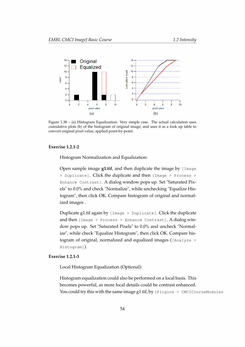
Equalization converts pixel values so that the values are distributed evenlywithin the dynamic range. Instead of describing this in detail using mathformula, I will explain it with a simple example (see Fig. 1.38). We con-sider an image with its pixel value ranging between 0 and 9. We plot thehistogram from this image, the result looks like in the figure 1.38a. Forequalization, a cumulative plot is first prepared from such histogram. Thiscumulative plot is computed by progressively integrating the histogramvalues (see Fig. 1.38b, black curve). To equalize (flatten) the pixel intensitydistribution within the range 0-9, we would ideally require a straight diag-onal cumulative plot (in other words, the probability density of the pixelintensity distribution should be near-flat). To get such plot, we need tocompensate the histogram by shifting values from the bars 5 and 7 to thebars 7 and 9, respectively (now, bars are in red after shifting). After thisshifting the cumulative plot now looks more straight and diagonal (Fig.1.38b right, red curve).
53
EMBL CMCI ImageJ Basic Course 1.2 Intensity
(a) (b)
Figure 1.38 – (a) Histogram Equalization: Very simple case. The actual calculation usescumulative plots (b) of the histogram of original image, and uses it as a look up table toconvert original pixel value, applied point-by-point.
Exercise 1.2.1-2
Histogram Normalization and Equalization:
Open sample image g1.tif, and then duplicate the image by [Image
> Duplicate]. Click the duplicate and then [Image > Process >
Enhance Contrast]. A dialog window pops up. Set "Saturated Pix-els" to 0.0% and check "Normalize", while unchecking "Equalize His-togram", then click OK. Compare histogram of original and normal-ized images .
Duplicate g1.tif again by [Image > Duplicate]. Click the duplicateand then [Image > Process > Enhance Contrast]. A dialog win-dow pops up. Set "Saturated Pixels" to 0.0% and uncheck "Normal-ize", while check "Equalize Histogram", then click OK. Compare his-togram of original, normalized and equalized images ([Analyze >
Histogram]).
Exercise 1.2.1-3
Local Histogram Equalization (Optional):
Histogram equalization could also be performed on a local basis. Thisbecomes powerful, as more local details could be contrast enhanced.You could try this with the same image g1.tif, by [Pligins > CMCICourseModules
54
EMBL CMCI ImageJ Basic Course 1.2 Intensity
> CLAHE] (if you have installed the course plugin in ImageJ) or if youare using Fiji, [Process > Enhance Local Contrast (CLAHE)]
1.2.2 Region of Interest (ROI)
To apply certain operation to a specific part of the image, you can select a re-gion by "region of interest (ROI)" tools. The shape of the ROI could be var-ious, such as rectangular, elliptical, polygon, free hand or a line (straight,segmented or free hand). There are several functions that will be used oftenin association with ROI tools.
Exercise 1.2.2-1
Cropping. Open any image. Select a region by rectangular ROI. Then[image > Crop]. This will remove the unnecessary part of the im-age, to reduce calculation time.
Exercise 1.2.2-2
Masking. Open any image. Select a region by rectangular ROI. Then[Edit > clear]. [Edit > Clear Outside]. After checking whathappened, do [Edit Fill]. (same operation could be done by [Edit> Selection > Crate Mask])
Exercise 1.2.2-3
Invert ROI. Open any image. Select a region by rectangular ROI. Then[Edit > Selection > Make Inverse]. In this way, you can selectregion excluding the region you initially selected.
Exercise 1.2.2-4
Redirecting ROI. Open any two images. In one of the image, select aregion by rectangular ROI. Then activate the other image by clickingthat window, and do [Edit > Selection > Restore Selection].ROI with same size and position will be reproduced in the window.
Exercise 1.2.2-5
ROI manager. You can store the position and size of the ROI in thememory. Select a region by rectangular ROI. Then [Analysis >
55
EMBL CMCI ImageJ Basic Course 1.2 Intensity
Tools > Roi Manager]. Click "Add" button to store ROI informa-tion. Stored ROI can be saved as a file, and could be loaded againwhen you restart the ImageJ.
1.2.3 Intensity Measurement
As you move the mouse pointer over individual pixels, their intensity valueare indicated in the ImageJ menu bar. This is the easiest way to read pixelintensities, but you can only get the values one by one. Here we learn away to get statistical information of a group of pixels within ROI. This hasmore practical usages for research.
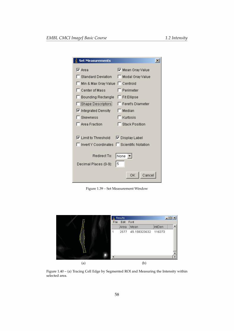
To measure pixel values of a ROI, ImageJ has a function [Analyze > Measure].Before using this function, you could specify the parameters you want tomeasure by [Analyze > Set measurements]. There are many parame-ters in the "Set measurement" window. Details on these parameters arelisted in the Appendix 1.6.4. For intensity measurements following param-eters are important.
• Mean Gray Value - Average gray value within the selection. This isthe sum of the gray values of all the pixels in the selection divided bythe number of pixels. Reported in calibrated units (e.g., optical den-sity) if Analyze/Calibrate was used to calibrate the image. For RGBimages, the mean is calculated by converting each pixel to grayscaleusing the formula gray = 0.299red+ 0.587green+ 0.114blue or the for-mula gray = (red+ green+ blue)/3 if "Unweighted RGB to GrayscaleConversion" is checked in Edit/Options/Conversions.
• Standard Deviation- Standard deviation of the gray values.
• Min & Max Gray Level - Minimum and maximum gray values withinthe selection.
• Integrated Density - The sum of the values of the pixels in the imageor selection. This is equivalent to the product of Area and Mean GrayValue. The Dot Blot Analysis example demonstrates how to use thismeasurement to analyze a dot blot assay.
56
EMBL CMCI ImageJ Basic Course 1.2 Intensity
A short note on image-based fluorometry: In biochemical experiments, sci-entists measure protein concentration by measuring absorbance of UV lightor by labeling proteins with dyes or fluorescence and measure the intensityof emission. This is because light absorbance or the intensity of fluores-cence intensity is proportional to the density of protein in the irradiatedvolume within cuvette. Very similar to this when fluorescence image ofcells are taken, pixel values (which is the fluorescence intensity) are pro-portional to the density of the labeled protein at each pixel positions. Forthis reason, measurement of fluorescence intensity using digital imagingcould be considered as the two dimensional version of the conventionalfluorometry.
Exercise 1.2.3-1
Open a sample image cells_Actin.tif. Before actually executing themeasurement, do [Analyze > Set Measurements]. A dialog win-dow opens. There are many parameters listed in the upper-half of thewindow.
The parameters we select now are:
• Area
• Integrated Density
• Mean Gray Value
Check the box of these three parameters. Integrated density is thesum of all the pixel values and Mean Gray Value is the average of allthe pixel values within ROI. So
IntegratedDensity = Area ∗MeanGrayValue
Select one of the cells in cell_Actin.tif image and zoom it up usingmagnifying tool. Switch the tool to "Polygon" tool. Draw polygonROI around the cell. Then do [Analyze > Measure]. A windowtitled "Results" pops-up, listing the measured values. Check that theintegrated density is the multiplication of area and the mean grayvalue.
This value is not the actual intensity of the fluorescence within the cellsince it also includes the background intensity (offset). Measure the
57
EMBL CMCI ImageJ Basic Course 1.2 Intensity
Figure 1.39 – Set Measurement Window
(a) (b)
Figure 1.40 – (a) Tracing Cell Edge by Segmented ROI and Measuring the Intensity withinselected area.
58
EMBL CMCI ImageJ Basic Course 1.2 Intensity
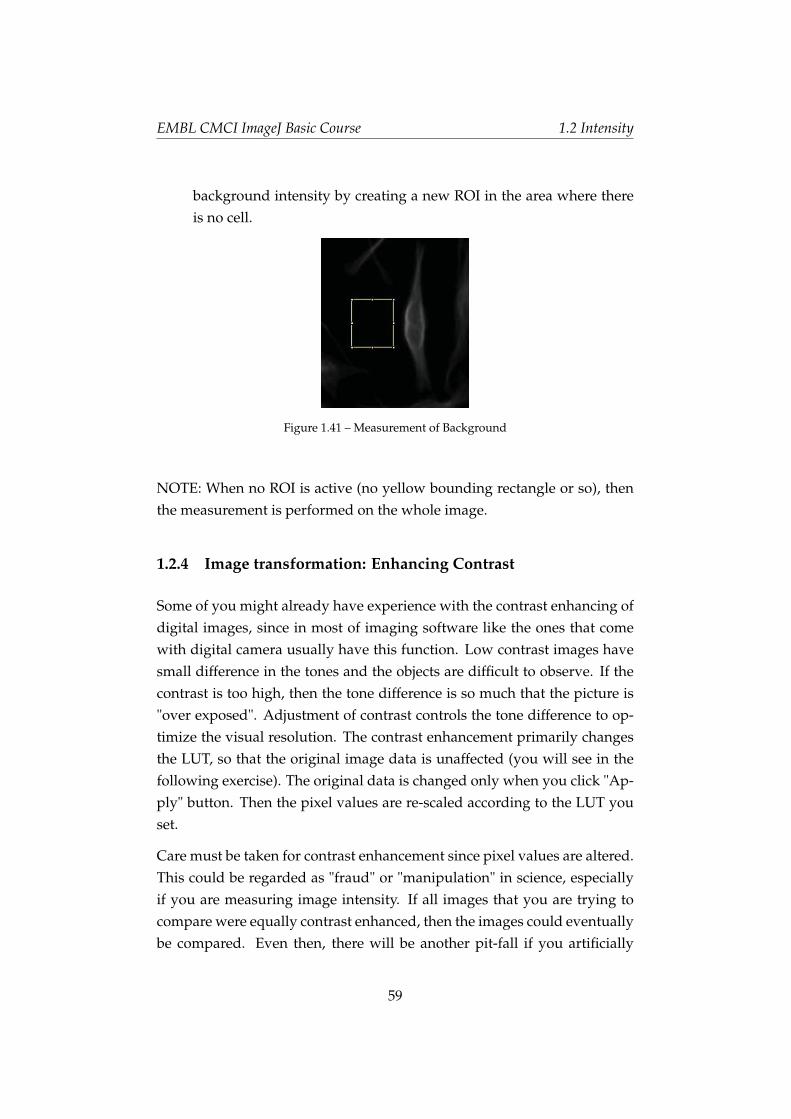
background intensity by creating a new ROI in the area where thereis no cell.
Figure 1.41 – Measurement of Background
NOTE: When no ROI is active (no yellow bounding rectangle or so), thenthe measurement is performed on the whole image.
1.2.4 Image transformation: Enhancing Contrast
Some of you might already have experience with the contrast enhancing ofdigital images, since in most of imaging software like the ones that comewith digital camera usually have this function. Low contrast images havesmall difference in the tones and the objects are difficult to observe. If thecontrast is too high, then the tone difference is so much that the picture is"over exposed". Adjustment of contrast controls the tone difference to op-timize the visual resolution. The contrast enhancement primarily changesthe LUT, so that the original image data is unaffected (you will see in thefollowing exercise). The original data is changed only when you click "Ap-ply" button. Then the pixel values are re-scaled according to the LUT youset.
Care must be taken for contrast enhancement since pixel values are altered.This could be regarded as "fraud" or "manipulation" in science, especiallyif you are measuring image intensity. If all images that you are trying tocompare were equally contrast enhanced, then the images could eventuallybe compared. Even then, there will be another pit-fall if you artificially
59
EMBL CMCI ImageJ Basic Course 1.2 Intensity
saturate the image: this happens often especially in the case of low bit-depth images.
Exercise 1.2.4-1
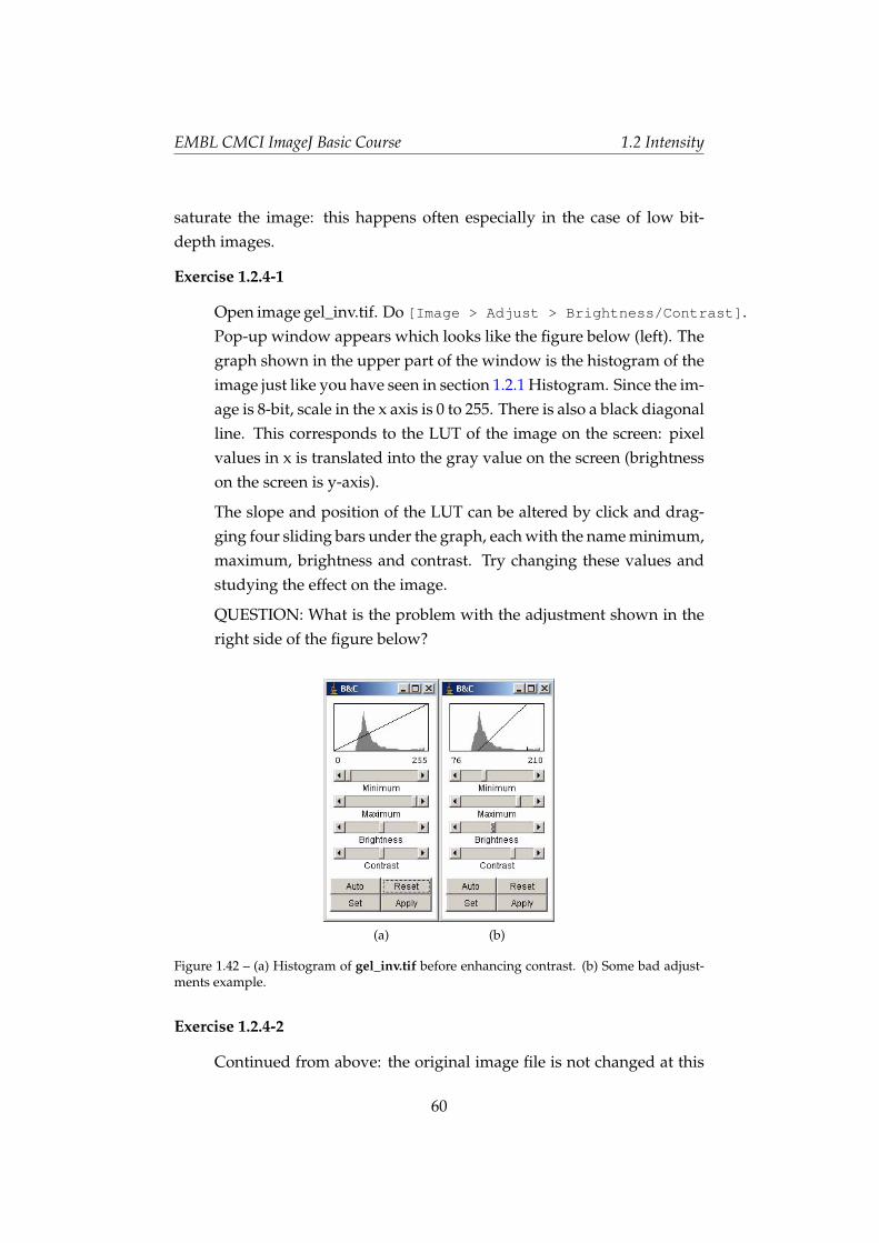
Open image gel_inv.tif. Do [Image > Adjust > Brightness/Contrast].Pop-up window appears which looks like the figure below (left). Thegraph shown in the upper part of the window is the histogram of theimage just like you have seen in section 1.2.1 Histogram. Since the im-age is 8-bit, scale in the x axis is 0 to 255. There is also a black diagonalline. This corresponds to the LUT of the image on the screen: pixelvalues in x is translated into the gray value on the screen (brightnesson the screen is y-axis).
The slope and position of the LUT can be altered by click and drag-ging four sliding bars under the graph, each with the name minimum,maximum, brightness and contrast. Try changing these values andstudying the effect on the image.
QUESTION: What is the problem with the adjustment shown in theright side of the figure below?
(a) (b)
Figure 1.42 – (a) Histogram of gel_inv.tif before enhancing contrast. (b) Some bad adjust-ments example.
Exercise 1.2.4-2
Continued from above: the original image file is not changed at this
60
EMBL CMCI ImageJ Basic Course 1.2 Intensity
stage. When you push "Apply" button at the bottom-right corner, theoriginal image is altered numerically. Try set the LUT as you like,and push the Apply: what happened to the Histogram and the LUTindicator? (you can always "Undo" the "Apply" by [Edit > Undo],or revert to the original file by [File > Revert]).
Exercise 1.2.4-3
With RGB image, it is possible to adjust the brightness and contrastfor individual color channel. Open the image RGB_cell.tif, then do[Image > Adjust > Color Balance]. There is a pull-down menuto specify the channel you want to change. Try changing differentchannels to optimize the image.
1.2.5 Image correlation between two images: co-localization plot
In many experiments we need to compare the localization of two or moreproteins and examine whether those proteins are co-localized. In manycases this has been evaluated by visual inspections. But with digital im-ages, it is possible to evaluate the degree of co-localization more quanti-tatively. This is done by plotting a so called "co-localization plot". To dothis in ImageJ one could download a plugin Colocalization_Finder11 andinstall it.
The level of colocalization could be then parametrized by using statisticalvalues such as Pearson’s coefficient and Mander’s coefficient. These val-ues have advantages and disadvantages depending on the image proper-ties. For detailed description on these issues, refer to Bolte and Cordelières(2006).
Additional insights, pitfalls and tips on localizing spot signals could befound in Waters (2009). This paper also provides detailed examination ofthe precision of dot detections.
11download from http://rsb.info.nih.gov/ij/plugins/colocalization-finder.html
61
EMBL CMCI ImageJ Basic Course 1.2 Intensity
1.2.6 ASSIGNMENTS
Assignment 1-2-1:
Suppose that you have an 8-bit grayscale image showing three objects ofdistinct intensities against a bright background. What would the corre-sponding histogram look like?
Assignment 1-2-2:
With image cell_Actin.tif, do the measurement with 4 cells and one back-ground in image as we did in the exercise. This time, store ROI in ROImanager (refer to 1.2.2 Roi) and do the measurement at once. First, youstore 5 different ROI one by one ("Add" button). Then click "Show all" but-ton in the ROI manager. Activate all ROI by clicking the ROI name in thelist while pushing down the SHIFT key. Then click "Measure" button. Allfive ROI will be measured at once. Average the values and describe theresults in text.
Assignment 1-2-3:
1. Optimize the contrast of image m51_8bit.tif. Be careful not to satu-rate the pixels so you don’t throw away important information in thelower pixel values. Check the histogram. Don’t close the histogramwindow
2. After applying the adjustment above (clicking "Apply" button), checkthe histogram again. Compare the histogram before and after. Whathappened? Discuss the reason.
62
EMBL CMCI ImageJ Basic Course 1.3 Filtering
1.3 Filtering
Filtering can improve the appearance of digital images. It can help identi-fying shapes by reducing the noise and enhancing the structural edge. Notonly for the appearance, filtering improve the efficiency of "segmentation"which we will study in the next section. Segmented image could be used asa mask to specify regions to be measured. Note that the filtering alters theimage so one must realize that in most cases, processed images cannot beused for quantitative intensity measurement without precise knowledge ofhow the processing affects the numerical values.
There are two different types of filtering: one involves the frequency do-main of images (Fourier transformed image), while the others deals withspatial domain. We first study the spatial filtering and its central concept"convolution", and walk through various types of convolutions. We thenstudy the frequency domain filtering (FFT). In the FFT world, convolutionof an image with filter kernel could be done simply by multiplication be-tween two images.
1.3.1 Convolution
In the [Process] menu, we see a long list of filters. Most of them arelinear filters and can be implemented as "convolution" as we will shortlysee. To perform a convolution a small mask (called kernel) is moved overthe image pixel by pixel and apply operations involving the surroundingpixel values (see Fig. 1.43). The result of operation is written to that pixelposition in the output image.
To understand how the convolution is done, we take a one-dimensionalexample (Fig. 1.44).
We have a small 1D array f , and we want to convolve a kernel w (i). Wefirst rotate the kernel by 180 degrees that the order is now reversed. Thenwe align f and w to match the position of the last element of kernel to thefirst element of f . Since we want to have all the kernel elements to havecorresponding partner, we "pad" f by 0. This is just for the convenience of
63
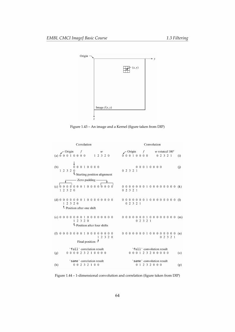
EMBL CMCI ImageJ Basic Course 1.3 Filtering
Figure 1.43 – An image and a Kernel (figure taken from DIP)
Figure 1.44 – 1-dimensional convolution and correlation (figure taken from DIP)
64
EMBL CMCI ImageJ Basic Course 1.3 Filtering
calculation (k). Then you multiply each element pairs (5 pairs in this case)and sum up the results. since all partners in f are 0, the sum of multiplica-tion is 0. We note this as the first element of "full convolution result" (o). Wethen slide w to the left by one element, do the multiplications and summingup again. Note the result as the second element of "full convolution result"(o). Like wise, we do such calculation step by step until last element of wmatches the last element of f (n). After that, we throw away padded ele-ments from the output 1D array to have a resulting array with same lengthas the original f (p).
To summarize, convolution is implemented sequentially as a local linearcombination of the input image using the filter kernel weights.
We do not use correlation in this course, but correlation is very much similarto convolution. In case of convolution the 1D kernel was rotated by 180degrees. In correlation, no rotation is done and used as it is and the rest ofthe algorithm is same. Correlation is often used for pattern matching to findout the pixel intensity distribution in an image using a template image as akernel. For example, many object tracking algorithm utilizes correlation forsearching target object from one frame to the other. In ImageJ, PIV (particleimage velocimetry) plugin12 uses the correlation to estimate motion vectorfield.
Convolution and correlation
Two closely-related bilinear operations that are especially im-portant for information processing are convolution and correlation.In the simplest case, correlation can be described as a compari-son of two fields at all possible relative positions. More specifi-cally, if χ is the correlation of two one-dimensional fields φ andψ, χ = φ ∗ ψ, then χ(r) reflects how well φ and ψ match (inan inner-product sense) when relatively displaced by r. Mathe-matically,
χ(r) =∫
Ωφ(s− r)ψ(s)ds
Higher dimensional correlations are the same, except that r is arelative displacement vector rather than a scalar.
12https://sites.google.com/site/qingzongtseng/piv
65
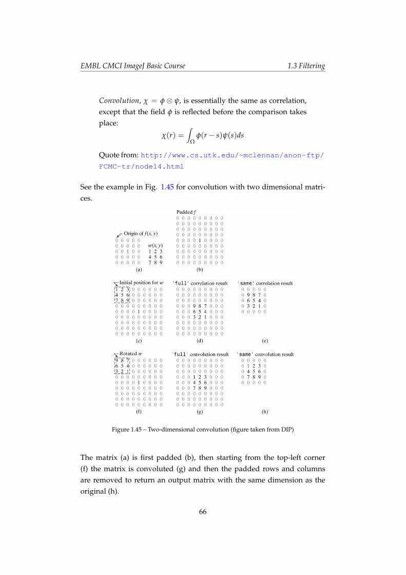
EMBL CMCI ImageJ Basic Course 1.3 Filtering
Convolution, χ = φ⊗ ψ, is essentially the same as correlation,except that the field φ is reflected before the comparison takesplace:
χ(r) =∫
Ωφ(r− s)ψ(s)ds
Quote from: http://www.cs.utk.edu/~mclennan/anon-ftp/FCMC-tr/node14.html
See the example in Fig. 1.45 for convolution with two dimensional matri-ces.
Figure 1.45 – Two-dimensional convolution (figure taken from DIP)
The matrix (a) is first padded (b), then starting from the top-left corner(f) the matrix is convoluted (g) and then the padded rows and columnsare removed to return an output matrix with the same dimension as theoriginal (h).
66
EMBL CMCI ImageJ Basic Course 1.3 Filtering
1.3.2 Kernels
In [Process] menu, we have many operators such as smooth, sharpen,find edges. . . and so on.
Many of them are called "linear filters", so called because filtering the sumof two equally sized images is equivalent to filtering these images apart andsumming the results. With non linear filters, these two different operationsmay end up in two different results13.
Smoothening
"Smoothening" operation, which is used for attenuating noise (Median ker-nel is better for shot-noise removal but for learning purpose we stick to thesmoothing), is done by applying the following kernel to the image.
1 1 11 1 11 1 1
Let’s take an example of an image with a vertical line in the middle.
0 0 10 0 00 0 10 0 00 0 10 0 00 0 10 0 00 0 10 0 0
Just for now, we forget about the padding for explanation, and first applythe kernel to the top-left corner for calculating convolved value at (1, 1)pixel position (note: top-left element position is (0, 0)). Then the calculationis
13This property is absolutely fundamental and at the heart of transform domain basedfiltering. For instance discrete Fourier transform decomposes any discrete signal (image) ina finite sum of components (images): knowing the effect of the filter on each of these finitecomponents is hence sufficient to fully characterize the filter and its effect on any signal(image)
67
EMBL CMCI ImageJ Basic Course 1.3 Filtering
output(1, 1)= (0× 1 + 0× 1 + 0× 1+
0× 1 + 0× 1 + 0× 1+10× 1 + 10× 1 + 10× 1)/9
= 30/9= 3
The sum of multiplication is divided by 9, which is the sum of all elementsin the kernel. This is to normalize the convolution, so that the output valuewill not to be too large compared to the original. We then shift the kernelone step in x-direction, and apply the kernel for calculating (2, 1) position.
output(2, 1)= (0× 1 + 0× 1 + 0× 1+
10× 1 + 10× 1 + 10× 1+0× 1 + 0× 1 + 0× 1)/9
= 30/9= 3
You might have now understood that the "smooth" operation is actuallyaveraging the values in the surrounding. Applying the kernel through theimage, the new image will be:
0 2 2 2 00 3 3 3 00 3 3 3 00 3 3 3 00 2 2 2 0
The vertical line is then now broader and darker – the smoothing effect.Note that the pixels in the first and the 5th rows were calculated with zeropadding so that values are 2 rather than 3. This is the boundary effectunavoidable with any filtering by convolution. We could attenuate thiseffect if we do padding by duplicating neighboring pixels. Then the resultof convolution then becomes
68
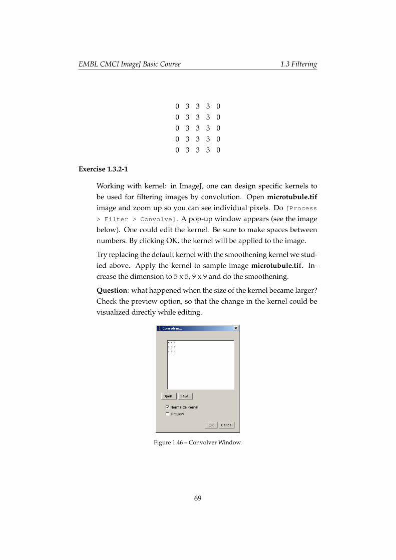
EMBL CMCI ImageJ Basic Course 1.3 Filtering
0 3 3 3 00 3 3 3 00 3 3 3 00 3 3 3 00 3 3 3 0
Exercise 1.3.2-1
Working with kernel: in ImageJ, one can design specific kernels tobe used for filtering images by convolution. Open microtubule.tifimage and zoom up so you can see individual pixels. Do [Process
> Filter > Convolve]. A pop-up window appears (see the imagebelow). One could edit the kernel. Be sure to make spaces betweennumbers. By clicking OK, the kernel will be applied to the image.
Try replacing the default kernel with the smoothening kernel we stud-ied above. Apply the kernel to sample image microtubule.tif. In-crease the dimension to 5 x 5, 9 x 9 and do the smoothening.
Question: what happened when the size of the kernel became larger?Check the preview option, so that the change in the kernel could bevisualized directly while editing.
Figure 1.46 – Convolver Window.
69
EMBL CMCI ImageJ Basic Course 1.3 Filtering
Sharpen
−1 −1 −1−1 12 −1−1 −1 −1
This kernel sharpens the image, also known as Laplacian. Side effect: noiseis also enhanced.
Find Edge (gradient)
The following two kernels are applied independently. Square root of thesum of the square of two result images will be calculated (called "SobelFilter": for more details, see Appendix 1.6.5)
1 2 10 0 0−1 −2 −1
and
1 0 −12 0 −21 0 −1
Gaussian Blur
This kernel blurs (in positive sense, we call it "smooth") the image by con-volution using a square Gaussian (bell-shaped) kernel. The width of thekernel, in pixels, is 2*sigma+1, where sigma is entered into a dialog box (Im-ageJ documentation). The following Gaussian kernels are respectively ob-tained for sigma equal 2 (5x5), 3 (7x7) and 7 (15x15).
Gauss 5 x 5 (Sigma = 2)
70

EMBL CMCI ImageJ Basic Course 1.3 Filtering
1 1 2 1 11 2 4 2 12 4 8 4 21 2 4 2 11 1 2 1 1
Gauss 7 x 7 (Sigma = 3)
1 1 1 2 1 1 11 2 2 4 2 2 12 2 4 8 4 2 22 4 8 16 8 4 22 2 4 8 4 2 21 2 2 4 2 2 11 1 1 2 1 1 1
Gauss 15 x 15 (Sigma = 7)
2 2 3 4 5 5 6 6 6 5 5 4 3 2 22 3 4 5 7 7 8 8 8 7 7 5 4 3 23 4 6 7 9 10 10 11 10 10 9 7 6 4 34 5 7 9 10 12 13 13 13 12 10 9 7 5 45 7 9 11 13 14 15 16 15 14 13 11 9 7 55 7 10 12 14 16 17 18 17 16 14 12 10 7 56 8 10 13 15 17 19 19 19 17 15 13 10 8 66 8 11 13 16 18 19 20 19 18 16 13 11 8 66 8 10 13 15 17 19 19 19 17 15 13 10 8 65 7 10 12 14 16 17 18 17 16 14 12 10 7 55 7 9 11 13 14 15 16 15 14 13 11 9 7 54 5 7 9 10 12 13 13 13 12 10 9 7 5 43 4 6 7 9 10 10 11 10 10 9 7 6 4 32 3 4 5 7 7 8 8 8 7 7 5 4 3 22 2 3 4 5 5 6 6 6 5 5 4 3 2 2
71
EMBL CMCI ImageJ Basic Course 1.3 Filtering
Median
None-linear filters are so called because the result of applying the filteris non-linear. Median filter used for the removal of noise is one of suchfilters. In ImageJ, the command will be [Process > Filter > Median].Following is the principle of how median filter works. When we applymedian filter with a 3 x 3 size, ImageJ samples 3 x 3 neighbors surroundingthe target pixel. Graphically, if the sampled region looks like below (targetposition contains 2 now)
1 7 94 2 86 5 3
Then we align these numbers in the ascending order.
1 2 3 4 5 6 7 8 9
We take the median of this sequence (= 5) and replace the value 2 with 5.
1.3.3 Morphological Image Processing
Mathematical morphology is a powerful tool that can be used to extractfeatures and components from an image. It is often used to pre-processor post-process images to facilitate a posterior analysis. In this process asmall shape (structuring element, not necessarily square like we did in theprecious section) is translated across the image during the course of pro-cessing. Certain mathematical logic operations are performed on the imageusing the structuring element to generate the processed image. In this sec-tion, we first introduce dilation and erosion, two fundamental operationsin mathematical morphology. We then describe morphological operationsobtained by combining erosion and dilation.
Dilation
Dilation is an operation that grows objects in a binary image. The thicken-ing is controlled by a small structuring element. In Fig. 1.47 you can see
72

EMBL CMCI ImageJ Basic Course 1.3 Filtering
the structuring element on the right and the result after applying dilationon a rectangle.
Erosion
Erosion shrinks or thins objects in a binary image. After erosion the onlypixels that survive are those where the structuring element fits entirely inthe foreground (Fig. 1.48).
In above examples the structuring elements are asymmetrically shaped. InImageJ, the structuring element used by the morphological filters of theProcess > Filters menu is a square so that the effects are even alongboth axes.
Exercise 1.3.3-1
Load noisy-fingerprint.tif and broken-text.tif. Apply dilation or ero-sion several times by setting the number of iterations.
To change this number use [Process > Binary > Options]. Bi-nary option window opens and you can set several parameters. "Count"matters with setting the number of overlapping pixels between struc-turing element and the object that determines output 0 or 1. Largercount causes less degree of erosion or dilation.
From ImageJ manual: Iterations specifies the number of timeserosion, dilation, opening, and closing are performed. Countspecifies the number of adjacent background pixels necessarybefore a pixel is removed from the edge of an object during ero-sion and the number of adjacent foreground pixels necessarybefore a pixel is added to the edge of an object during dilation.Check Black Background if the image has white objects on ablack background.
73
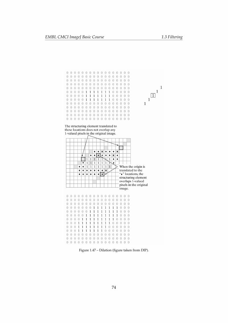
EMBL CMCI ImageJ Basic Course 1.3 Filtering
Figure 1.47 – Dilation (figure taken from DIP).
74

EMBL CMCI ImageJ Basic Course 1.3 Filtering
Figure 1.48 – Erosion (figure taken from DIP)
75
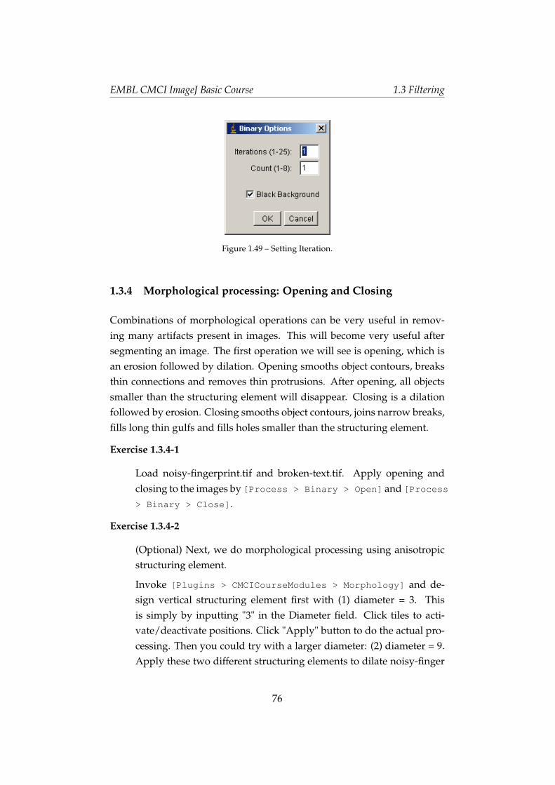
EMBL CMCI ImageJ Basic Course 1.3 Filtering
Figure 1.49 – Setting Iteration.
1.3.4 Morphological processing: Opening and Closing
Combinations of morphological operations can be very useful in remov-ing many artifacts present in images. This will become very useful aftersegmenting an image. The first operation we will see is opening, which isan erosion followed by dilation. Opening smooths object contours, breaksthin connections and removes thin protrusions. After opening, all objectssmaller than the structuring element will disappear. Closing is a dilationfollowed by erosion. Closing smooths object contours, joins narrow breaks,fills long thin gulfs and fills holes smaller than the structuring element.
Exercise 1.3.4-1
Load noisy-fingerprint.tif and broken-text.tif. Apply opening andclosing to the images by [Process > Binary > Open] and [Process
> Binary > Close].
Exercise 1.3.4-2
(Optional) Next, we do morphological processing using anisotropicstructuring element.
Invoke [Plugins > CMCICourseModules > Morphology] and de-sign vertical structuring element first with (1) diameter = 3. Thisis simply by inputting "3" in the Diameter field. Click tiles to acti-vate/deactivate positions. Click "Apply" button to do the actual pro-cessing. Then you could try with a larger diameter: (2) diameter = 9.Apply these two different structuring elements to dilate noisy-finger
76
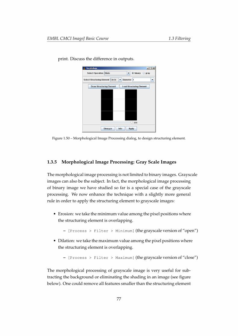
EMBL CMCI ImageJ Basic Course 1.3 Filtering
print. Discuss the difference in outputs.
Figure 1.50 – Morphological Image Processing dialog, to design structuring element.
1.3.5 Morphological Image Processing: Gray Scale Images
The morphological image processing is not limited to binary images. Grayscaleimages can also be the subject. In fact, the morphological image processingof binary image we have studied so far is a special case of the grayscaleprocessing. We now enhance the technique with a slightly more generalrule in order to apply the structuring element to grayscale images:
• Erosion: we take the minimum value among the pixel positions wherethe structuring element is overlapping.
– [Process > Filter > Minimum] (the grayscale version of “open”)
• Dilation: we take the maximum value among the pixel positions wherethe structuring element is overlapping.
– [Process > Filter > Maximum] (the grayscale version of “close”)
The morphological processing of grayscale image is very useful for sub-tracting the background or eliminating the shading in an image (see figurebelow). One could remove all features smaller than the structuring element
77
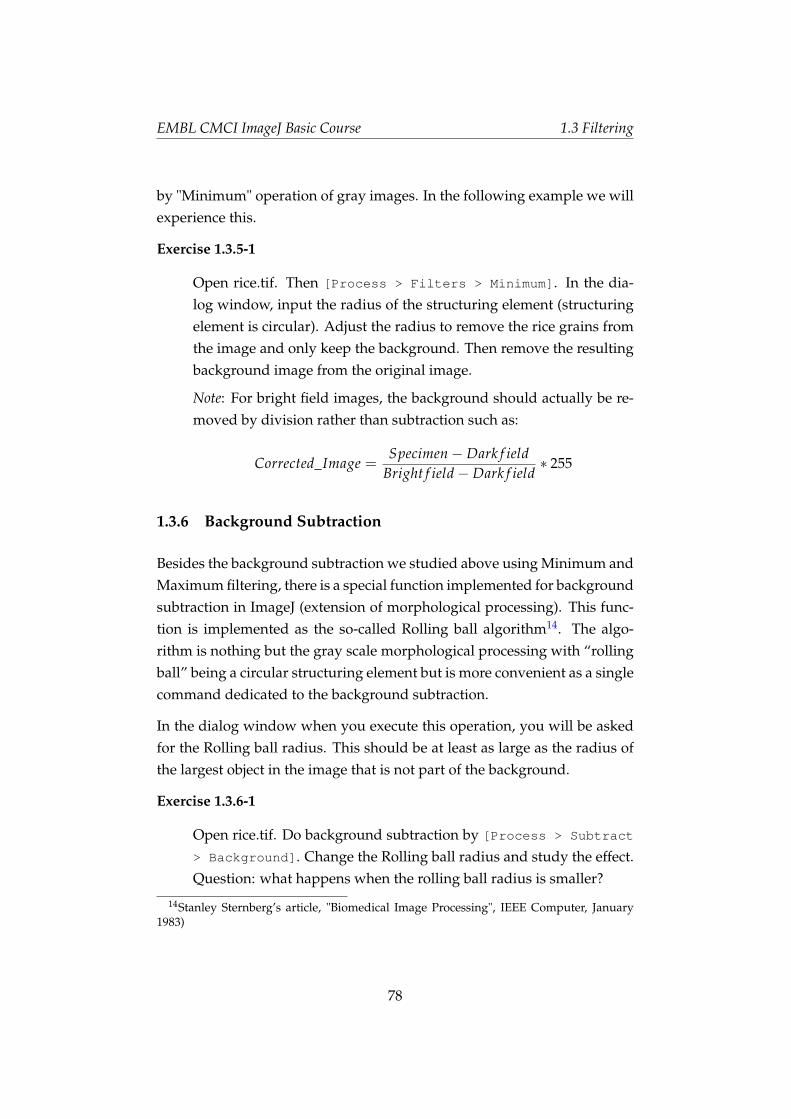
EMBL CMCI ImageJ Basic Course 1.3 Filtering
by "Minimum" operation of gray images. In the following example we willexperience this.
Exercise 1.3.5-1
Open rice.tif. Then [Process > Filters > Minimum]. In the dia-log window, input the radius of the structuring element (structuringelement is circular). Adjust the radius to remove the rice grains fromthe image and only keep the background. Then remove the resultingbackground image from the original image.
Note: For bright field images, the background should actually be re-moved by division rather than subtraction such as:
Corrected_Image =Specimen− Dark f ield
Bright f ield− Dark f ield∗ 255
1.3.6 Background Subtraction
Besides the background subtraction we studied above using Minimum andMaximum filtering, there is a special function implemented for backgroundsubtraction in ImageJ (extension of morphological processing). This func-tion is implemented as the so-called Rolling ball algorithm14. The algo-rithm is nothing but the gray scale morphological processing with “rollingball” being a circular structuring element but is more convenient as a singlecommand dedicated to the background subtraction.
In the dialog window when you execute this operation, you will be askedfor the Rolling ball radius. This should be at least as large as the radius ofthe largest object in the image that is not part of the background.
Exercise 1.3.6-1
Open rice.tif. Do background subtraction by [Process > Subtract
> Background]. Change the Rolling ball radius and study the effect.Question: what happens when the rolling ball radius is smaller?
14Stanley Sternberg’s article, "Biomedical Image Processing", IEEE Computer, January1983)
78
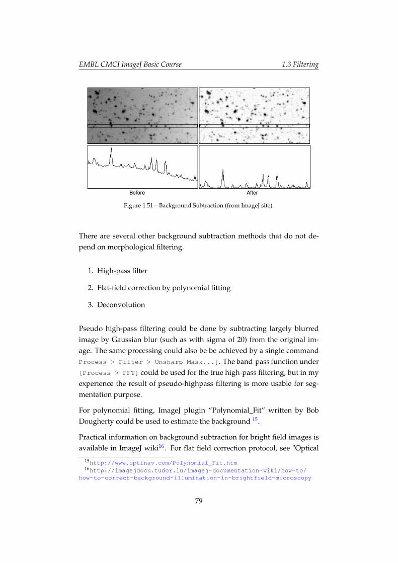
EMBL CMCI ImageJ Basic Course 1.3 Filtering
Figure 1.51 – Background Subtraction (from ImageJ site).
There are several other background subtraction methods that do not de-pend on morphological filtering.
1. High-pass filter
2. Flat-field correction by polynomial fitting
3. Deconvolution
Pseudo high-pass filtering could be done by subtracting largely blurredimage by Gaussian blur (such as with sigma of 20) from the original im-age. The same processing could also be be achieved by a single commandProcess > Filter > Unsharp Mask...]. The band-pass function under[Process > FFT] could be used for the true high-pass filtering, but in myexperience the result of pseudo-highpass filtering is more usable for seg-mentation purpose.
For polynomial fitting, ImageJ plugin “Polynomial_Fit” written by BobDougherty could be used to estimate the background 15.
Practical information on background subtraction for bright field images isavailable in ImageJ wiki16. For flat field correction protocol, see "Optical
15http://www.optinav.com/Polynomial_Fit.htm16http://imagejdocu.tudor.lu/imagej-documentation-wiki/how-to/
how-to-correct-background-illumination-in-brightfield-microscopy
79

EMBL CMCI ImageJ Basic Course 1.3 Filtering
Microscopy Primer" site17.
Protocol for the background subtraction for fluorescence images using cal-ibration slide and ImageJ could be found in Miura and Rietdorf (2006).
For the background removal of fluorescence time series, bleaching of flu-orescence should also be considered. See recent article by Schwarzfischeret al. (2011).
Deconvolution removes out-of-focus emission signal. See appendix 8 foran extensive tutorial using ImageJ plugin. You could also refer to a classicreview (Wallace et al., 2001).
1.3.7 Other Functions: Fill holes, Skeltonize, Outline
Frequently, after some morphological operation we need to fill the holes ina binary image. For example, we detect the boundary of a cell and want toobtain an object which is filled and covers the cell. In this example we willsee its effect.
Exercise 1.3.7-1
Open book-text.tif. Then fill holes by [Process > Binary > Fill
Holes].
17http://micro.magnet.fsu.edu/primer/digitalimaging/imageprocessingintro.html
80
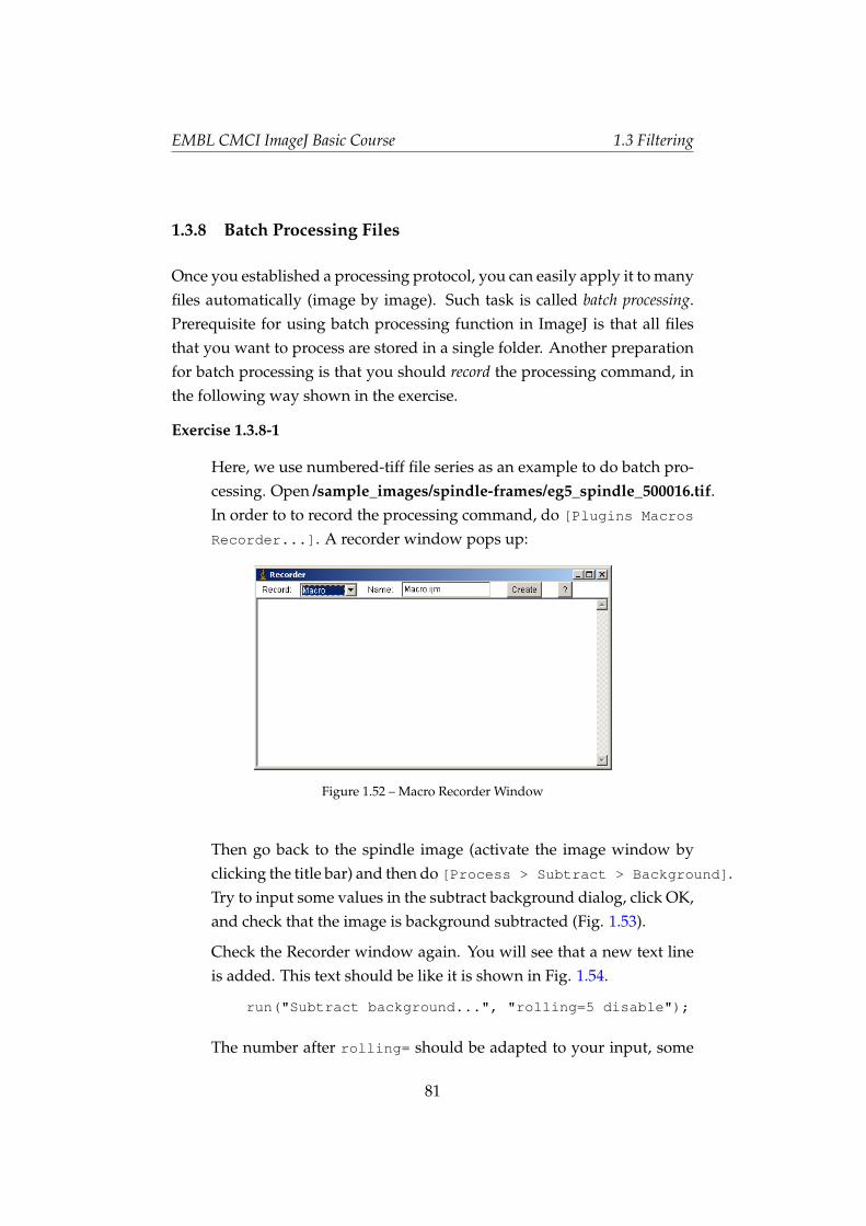
EMBL CMCI ImageJ Basic Course 1.3 Filtering
1.3.8 Batch Processing Files
Once you established a processing protocol, you can easily apply it to manyfiles automatically (image by image). Such task is called batch processing.Prerequisite for using batch processing function in ImageJ is that all filesthat you want to process are stored in a single folder. Another preparationfor batch processing is that you should record the processing command, inthe following way shown in the exercise.
Exercise 1.3.8-1
Here, we use numbered-tiff file series as an example to do batch pro-cessing. Open /sample_images/spindle-frames/eg5_spindle_500016.tif.In order to to record the processing command, do [Plugins Macros
Recorder...]. A recorder window pops up:
Figure 1.52 – Macro Recorder Window
Then go back to the spindle image (activate the image window byclicking the title bar) and then do [Process > Subtract > Background].Try to input some values in the subtract background dialog, click OK,and check that the image is background subtracted (Fig. 1.53).
Check the Recorder window again. You will see that a new text lineis added. This text should be like it is shown in Fig. 1.54.
run("Subtract background...", "rolling=5 disable");
The number after rolling= should be adapted to your input, some
81
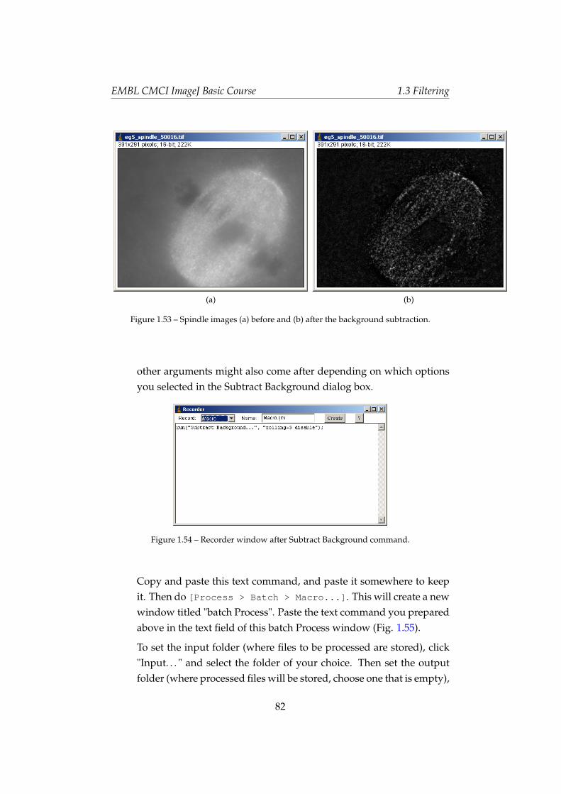
EMBL CMCI ImageJ Basic Course 1.3 Filtering
(a) (b)
Figure 1.53 – Spindle images (a) before and (b) after the background subtraction.
other arguments might also come after depending on which optionsyou selected in the Subtract Background dialog box.
Figure 1.54 – Recorder window after Subtract Background command.
Copy and paste this text command, and paste it somewhere to keepit. Then do [Process > Batch > Macro...]. This will create a newwindow titled "batch Process". Paste the text command you preparedabove in the text field of this batch Process window (Fig. 1.55).
To set the input folder (where files to be processed are stored), click"Input. . . " and select the folder of your choice. Then set the outputfolder (where processed files will be stored, choose one that is empty),
82
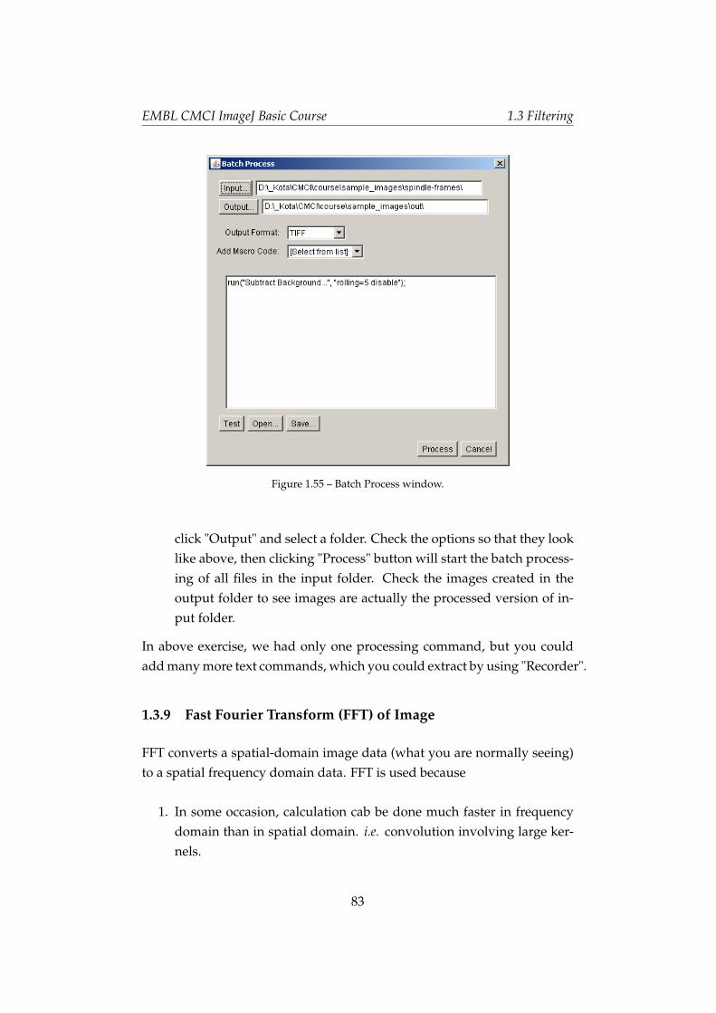
EMBL CMCI ImageJ Basic Course 1.3 Filtering
Figure 1.55 – Batch Process window.
click "Output" and select a folder. Check the options so that they looklike above, then clicking "Process" button will start the batch process-ing of all files in the input folder. Check the images created in theoutput folder to see images are actually the processed version of in-put folder.
In above exercise, we had only one processing command, but you couldadd many more text commands, which you could extract by using "Recorder".
1.3.9 Fast Fourier Transform (FFT) of Image
FFT converts a spatial-domain image data (what you are normally seeing)to a spatial frequency domain data. FFT is used because
1. In some occasion, calculation cab be done much faster in frequencydomain than in spatial domain. i.e. convolution involving large ker-nels.
83
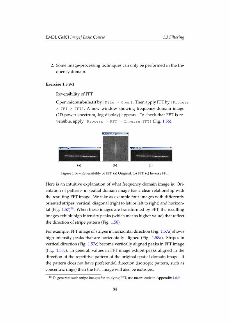
EMBL CMCI ImageJ Basic Course 1.3 Filtering
2. Some image-processing techniques can only be performed in the fre-quency domain.
Exercise 1.3.9-1
Reversibility of FFT
Open microtubule.tif by [File > Open]. Then apply FFT by [Process> FFT > FFT]. A new window showing frequency-domain image(2D power spectrum, log display) appears. To check that FFT is re-versible, apply [Process > FFT > Inverse FFT] (Fig. 1.56).
(a) (b) (c)
Figure 1.56 – Reversibility of FFT. (a) Original, (b) FFT, (c) Inverse FFT.
Here is an intuitive explanation of what frequency domain image is: Ori-entation of patterns in spatial domain image has a clear relationship withthe resulting FFT image. We take as example four images with differentlyoriented stripes, vertical, diagonal (right to left or left to right) and horizon-tal (Fig. 1.57)18. When these images are transformed by FFT, the resultingimages exhibit high intensity peaks (which means higher value) that reflectthe direction of stripe pattern (Fig. 1.58).
For example, FFT image of stripes in horizontal direction (Fig. 1.57a) showshigh intensity peaks that are horizontally aligned (Fig. 1.58a). Stripes invertical direction (Fig. 1.57c) become vertically aligned peaks in FFT image(Fig. 1.58c). In general, values in FFT image exhibit peaks aligned in thedirection of the repetitive pattern of the original spatial-domain image. Ifthe pattern does not have preferential direction (isotropic pattern, such asconcentric rings) then the FFT image will also be isotropic.
18 To generate such stripe images for studying FFT, use macro code in Appendix 1.6.9.
84
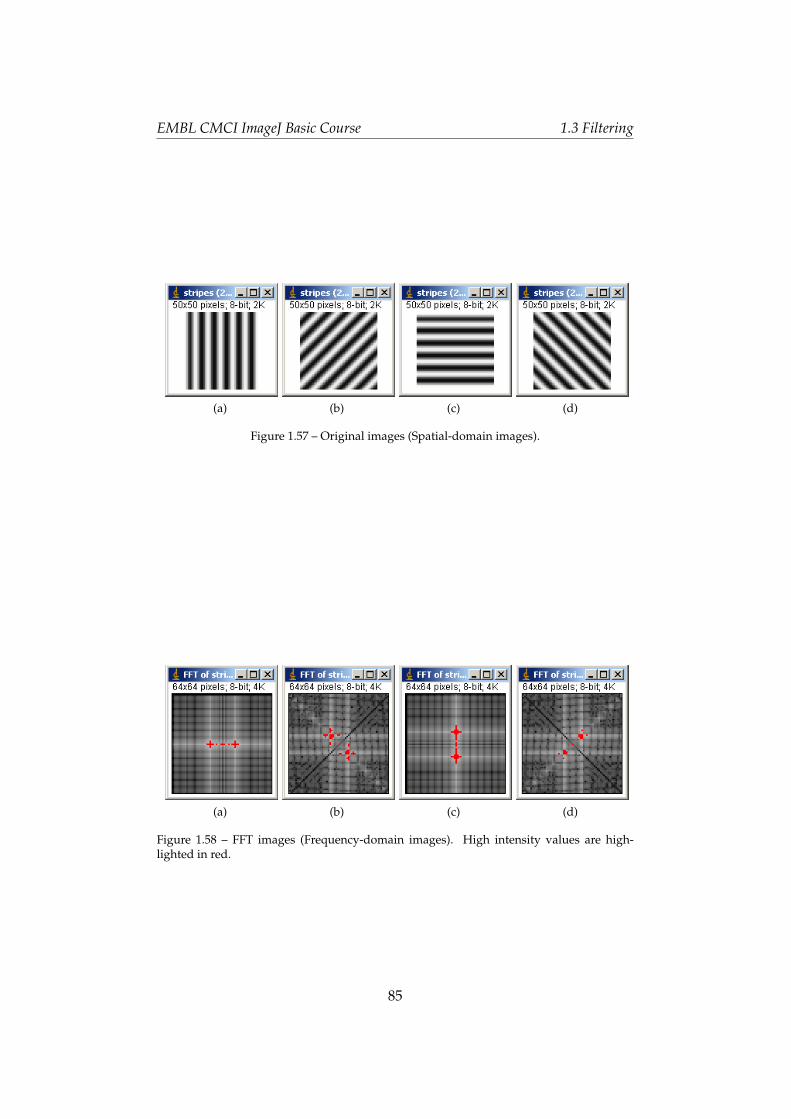
EMBL CMCI ImageJ Basic Course 1.3 Filtering
(a) (b) (c) (d)
Figure 1.57 – Original images (Spatial-domain images).
(a) (b) (c) (d)
Figure 1.58 – FFT images (Frequency-domain images). High intensity values are high-lighted in red.
85
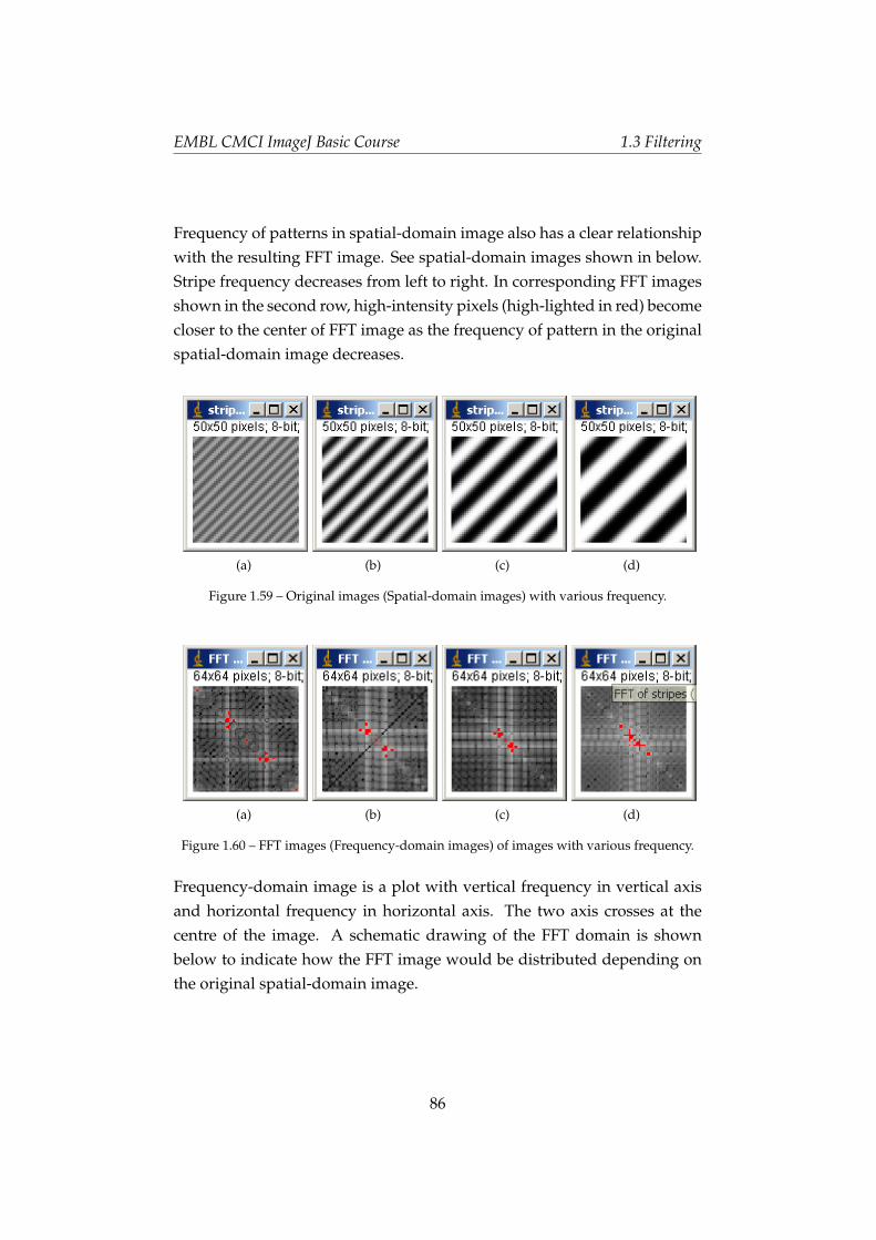
EMBL CMCI ImageJ Basic Course 1.3 Filtering
Frequency of patterns in spatial-domain image also has a clear relationshipwith the resulting FFT image. See spatial-domain images shown in below.Stripe frequency decreases from left to right. In corresponding FFT imagesshown in the second row, high-intensity pixels (high-lighted in red) becomecloser to the center of FFT image as the frequency of pattern in the originalspatial-domain image decreases.
(a) (b) (c) (d)
Figure 1.59 – Original images (Spatial-domain images) with various frequency.
(a) (b) (c) (d)
Figure 1.60 – FFT images (Frequency-domain images) of images with various frequency.
Frequency-domain image is a plot with vertical frequency in vertical axisand horizontal frequency in horizontal axis. The two axis crosses at thecentre of the image. A schematic drawing of the FFT domain is shownbelow to indicate how the FFT image would be distributed depending onthe original spatial-domain image.
86
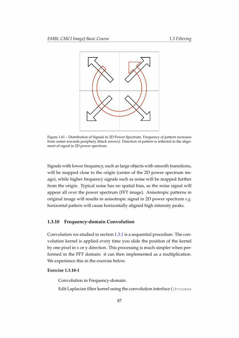
EMBL CMCI ImageJ Basic Course 1.3 Filtering
Figure 1.61 – Distribution of Signals in 2D Power Spectrum. Frequency of pattern increasesfrom center towards periphery (black arrows). Direction of pattern is reflected in the align-ment of signal in 2D power spectrum.
Signals with lower frequency, such as large objects with smooth transitions,will be mapped close to the origin (center of the 2D power spectrum im-age), while higher frequency signals such as noise will be mapped furtherfrom the origin. Typical noise has no spatial bias, so the noise signal willappear all over the power spectrum (FFT image). Anisotropic patterns inoriginal image will results in anisotropic signal in 2D power spectrum e.g.horizontal pattern will cause horizontally aligned high intensity peaks.
1.3.10 Frequency-domain Convolution
Convolution we studied in section 1.3.1 is a sequential procedure. The con-volution kernel is applied every time you slide the position of the kernelby one pixel in x or y direction. This processing is much simpler when per-formed in the FFT domain: it can then implemented as a multiplication.We experience this in the exercise below.
Exercise 1.3.10-1
Convolution in Frequency-domain.
Edit Laplacian filter kernel using the convolution interface ([Process
87
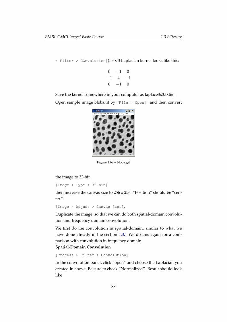
EMBL CMCI ImageJ Basic Course 1.3 Filtering
> Filter > COnvolution]). 3 x 3 Laplacian kernel looks like this:
0 −1 0−1 4 −10 −1 0
Save the kernel somewhere in your computer as laplace3x3.txt.
Open sample image blobs.tif by [File > Open]. and then convert
Figure 1.62 – blobs.gif
the image to 32-bit.
[Image > Type > 32-bit]
then increase the canvas size to 256 x 256. “Position” should be “cen-ter”.
[Image > Adjust > Canvas Size].
Duplicate the image, so that we can do both spatial-domain convolu-tion and frequency domain convolution.
We first do the convolution in spatial-domain, similar to what wehave done already in the section 1.3.1 We do this again for a com-parison with convolution in frequency domain.Spatial-Domain Convolution
[Process > Filter > Convolution]
In the convolution panel, click “open” and choose the Laplacian youcreated in above. Be sure to check “Normalized”. Result should looklike
88
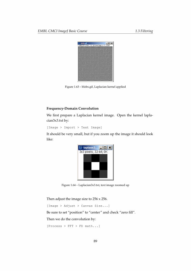
EMBL CMCI ImageJ Basic Course 1.3 Filtering
Figure 1.63 – blobs.gif, Laplacian kernel applied
Frequency-Domain Convolution
We first prepare a Laplacian kernel image. Open the kernel lapla-cian3x3.txt by:
[Image > Import > Text Image]
It should be very small, but if you zoom up the image it should looklike:
Figure 1.64 – Laplacian3x3.txt, text image zoomed up
Then adjust the image size to 256 x 256.
[Image > Adjust > Canvas Size...]
Be sure to set “position” to “center” and check “zero fill”.
Then we do the convolution by:
[Process > FFT > FD math...]
89
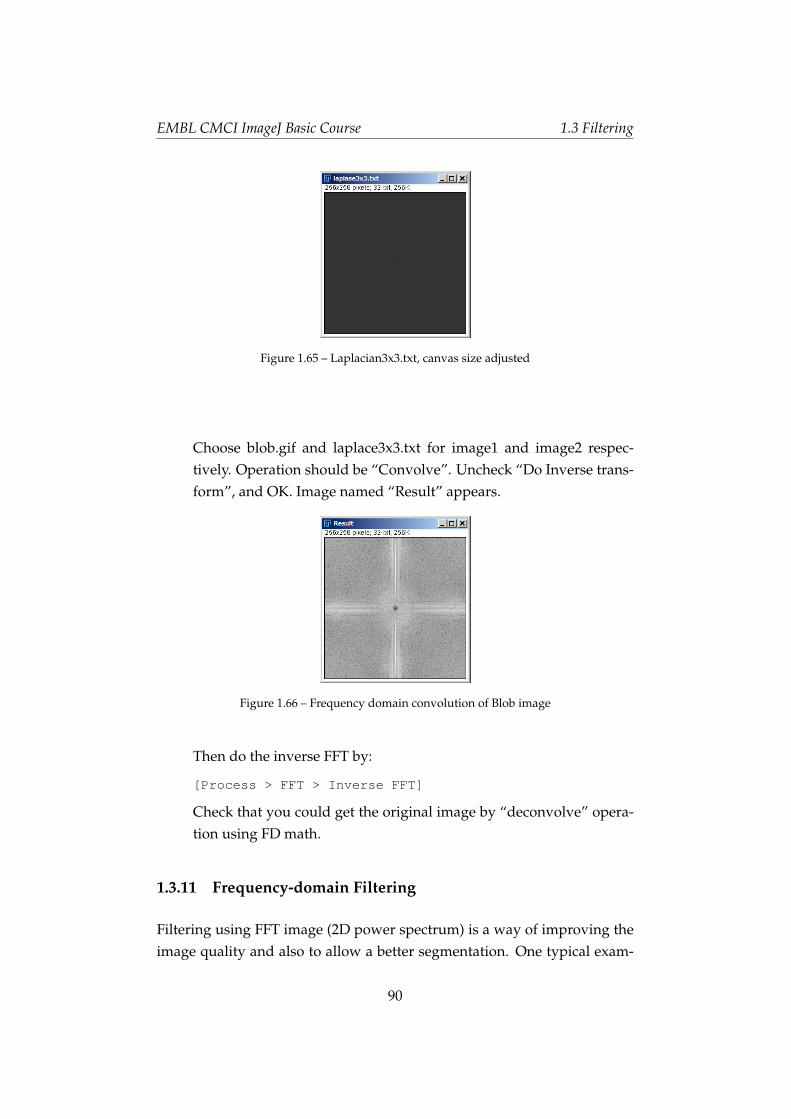
EMBL CMCI ImageJ Basic Course 1.3 Filtering
Figure 1.65 – Laplacian3x3.txt, canvas size adjusted
Choose blob.gif and laplace3x3.txt for image1 and image2 respec-tively. Operation should be “Convolve”. Uncheck “Do Inverse trans-form”, and OK. Image named “Result” appears.
Figure 1.66 – Frequency domain convolution of Blob image
Then do the inverse FFT by:
[Process > FFT > Inverse FFT]
Check that you could get the original image by “deconvolve” opera-tion using FD math.
1.3.11 Frequency-domain Filtering
Filtering using FFT image (2D power spectrum) is a way of improving theimage quality and also to allow a better segmentation. One typical exam-
90
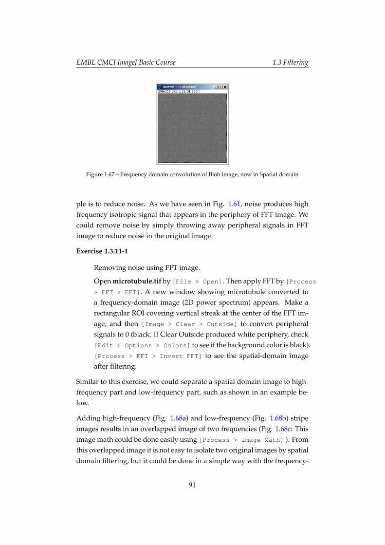
EMBL CMCI ImageJ Basic Course 1.3 Filtering
Figure 1.67 – Frequency domain convolution of Blob image, now in Spatial domain
ple is to reduce noise. As we have seen in Fig. 1.61, noise produces highfrequency isotropic signal that appears in the periphery of FFT image. Wecould remove noise by simply throwing away peripheral signals in FFTimage to reduce noise in the original image.
Exercise 1.3.11-1
Removing noise using FFT image.
Open microtubule.tif by [File > Open]. Then apply FFT by [Process> FFT > FFT]. A new window showing microtubule converted toa frequency-domain image (2D power spectrum) appears. Make arectangular ROI covering vertical streak at the center of the FFT im-age, and then [Image > Clear > Outside] to convert peripheralsignals to 0 (black. If Clear Outside produced white periphery, check[Edit > Options > Colors] to see if the background color is black).[Process > FFT > Invert FFT] to see the spatial-domain imageafter filtering.
Similar to this exercise, we could separate a spatial domain image to high-frequency part and low-frequency part, such as shown in an example be-low.
Adding high-frequency (Fig. 1.68a) and low-frequency (Fig. 1.68b) stripeimages results in an overlapped image of two frequencies (Fig. 1.68c: Thisimage math could be done easily using [Process > Image Math] ). Fromthis overlapped image it is not easy to isolate two original images by spatialdomain filtering, but it could be done in a simple way with the frequency-
91
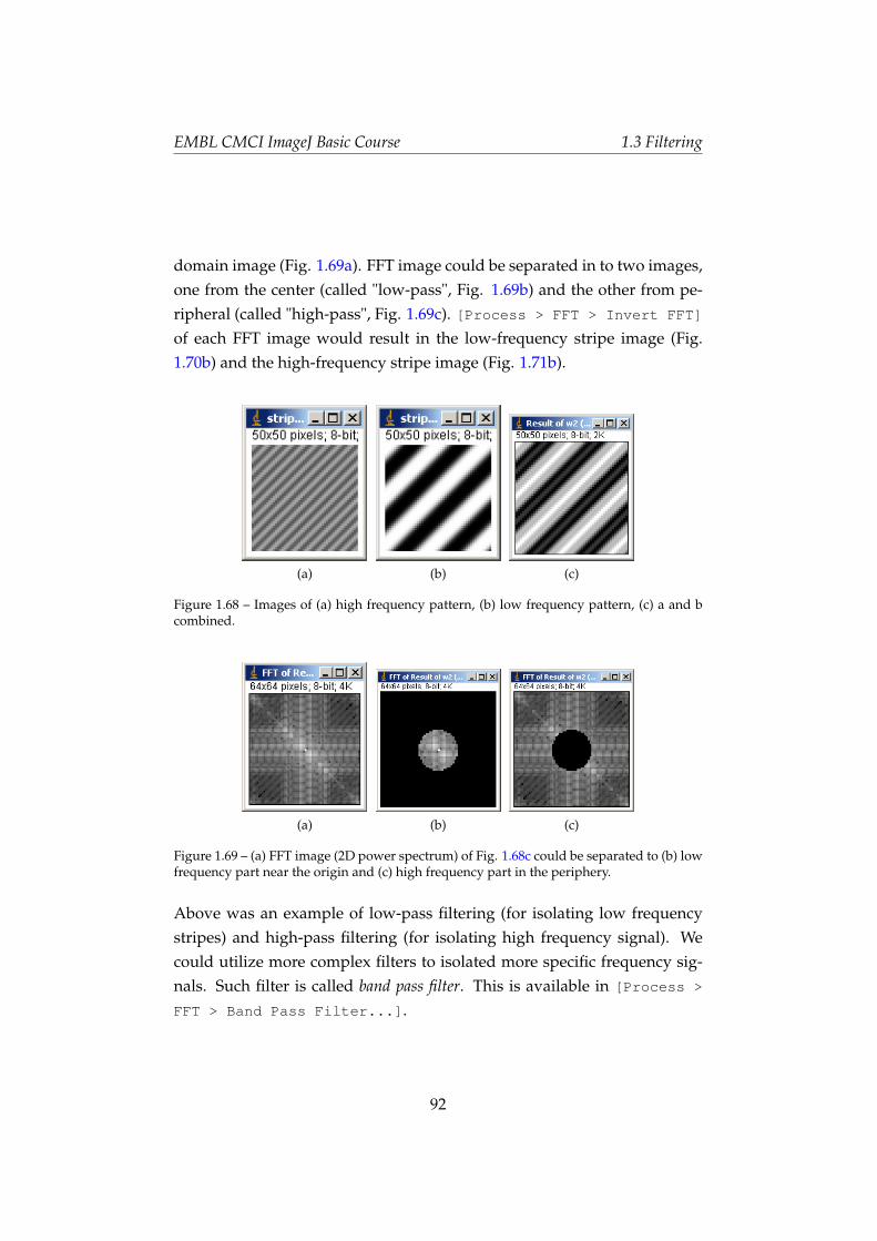
EMBL CMCI ImageJ Basic Course 1.3 Filtering
domain image (Fig. 1.69a). FFT image could be separated in to two images,one from the center (called "low-pass", Fig. 1.69b) and the other from pe-ripheral (called "high-pass", Fig. 1.69c). [Process > FFT > Invert FFT]
of each FFT image would result in the low-frequency stripe image (Fig.1.70b) and the high-frequency stripe image (Fig. 1.71b).
(a) (b) (c)
Figure 1.68 – Images of (a) high frequency pattern, (b) low frequency pattern, (c) a and bcombined.
(a) (b) (c)
Figure 1.69 – (a) FFT image (2D power spectrum) of Fig. 1.68c could be separated to (b) lowfrequency part near the origin and (c) high frequency part in the periphery.
Above was an example of low-pass filtering (for isolating low frequencystripes) and high-pass filtering (for isolating high frequency signal). Wecould utilize more complex filters to isolated more specific frequency sig-nals. Such filter is called band pass filter. This is available in [Process >
FFT > Band Pass Filter...].
92
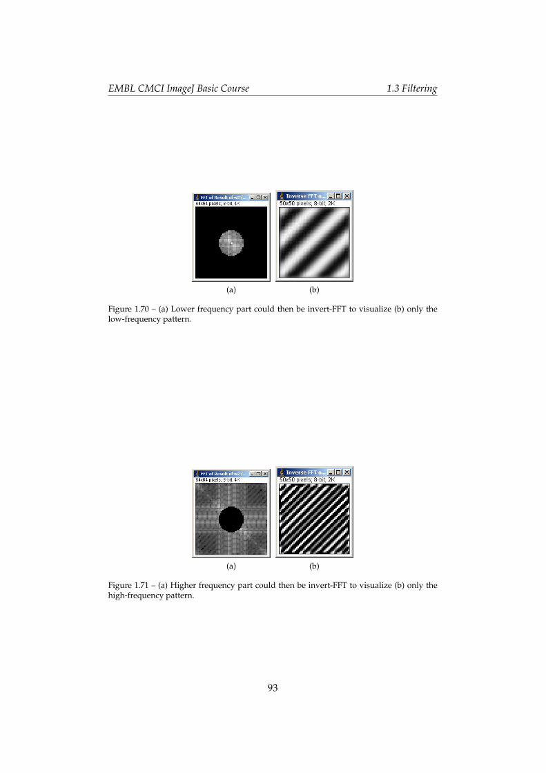
EMBL CMCI ImageJ Basic Course 1.3 Filtering
(a) (b)
Figure 1.70 – (a) Lower frequency part could then be invert-FFT to visualize (b) only thelow-frequency pattern.
(a) (b)
Figure 1.71 – (a) Higher frequency part could then be invert-FFT to visualize (b) only thehigh-frequency pattern.
93

EMBL CMCI ImageJ Basic Course 1.3 Filtering
1.3.12 ASSIGNMENTS
Assignment 1-3-1: Convolution and Kernels
1. Design your own kernel, apply it to an image of your choice and dis-cuss what it does.
2. Gaussian kernel: Open the Gaussian kernels (in sample image folder,Gss5x5.txt, Gss7x7.txt and Gss15x15.txt) by [File > Import > Text
Image]. Then try getting the line profile of 2D Gaussian, crossing thepeak of the curve. The line profile across the 2D Gaussian should be1-D Gaussian curve. Save the resulting graphs as image files.
3. Visualize the Gaussian kernel using the "surface plot" [Analyze >
Surface Plots...].
Assignment 1-3-2: Morphological Image Processing
Load example image [EMBL > Smaple Images> NPC-T01.tif]. Split chan-nels and work on nucleus channel in te following (red channel). Design animage processing protocol to create a binary image of nucleus boundary.Write down the protocol as a flow chart and also show the resulting image.
some important tips:
• use [Process > Binary > Convert to Mask]
• use erosion, dilation and image calculator.
94
EMBL CMCI ImageJ Basic Course 1.4 Segmentation
1.4 Segmentation
Segmentation refers to the process in which an image is subdivided intoconstituent regions or objects. These objects can be further processed oranalyzed for the extraction of quantitative information. Biological imagedata is usually messy and noisy, and as a result difficult to segment prop-erly. Multiple image pre-processing steps are often required to allow a goodsegmentation. We often combine segmentation with various morphologi-cal processing and filtering techniques (such as the ones described in theprevious section) to achieve an accurate and robust segmentation of an im-age. Image segmentation algorithms are generally based on one of two ba-sic properties of intensity values: discontinuity and similarity. In the firstcategory, the approach is to partition an image based on abrupt changesin intensity, edge-detection algorithms falls in this category. In the secondapproach, an image is partitioned into regions that are similar according toset of predefined criteria. Thresholding and watershed segmentation fall inthis category.
1.4.1 Thresholding
Many biological images comprise of light objects over a constant dark back-ground (especially those obtained using fluorescence microscopy), in sucha way that object and background pixels have gray levels grouped into twodominant modes. One obvious way to extract the objects from its back-ground is to select a threshold T that separates these modes:
g(x, y) =
1 if f (x, y) > T
0 otherwise(1.8)
Where g(x, y) is the thresholded image of f (x, y).
In a sense, thresholding is an extreme case of contrast enhancement westudied already (1.2.4). By setting a threshold value T and converting theimage, pixels with values above T becomes white and otherwise black(color could be in inverse).
95
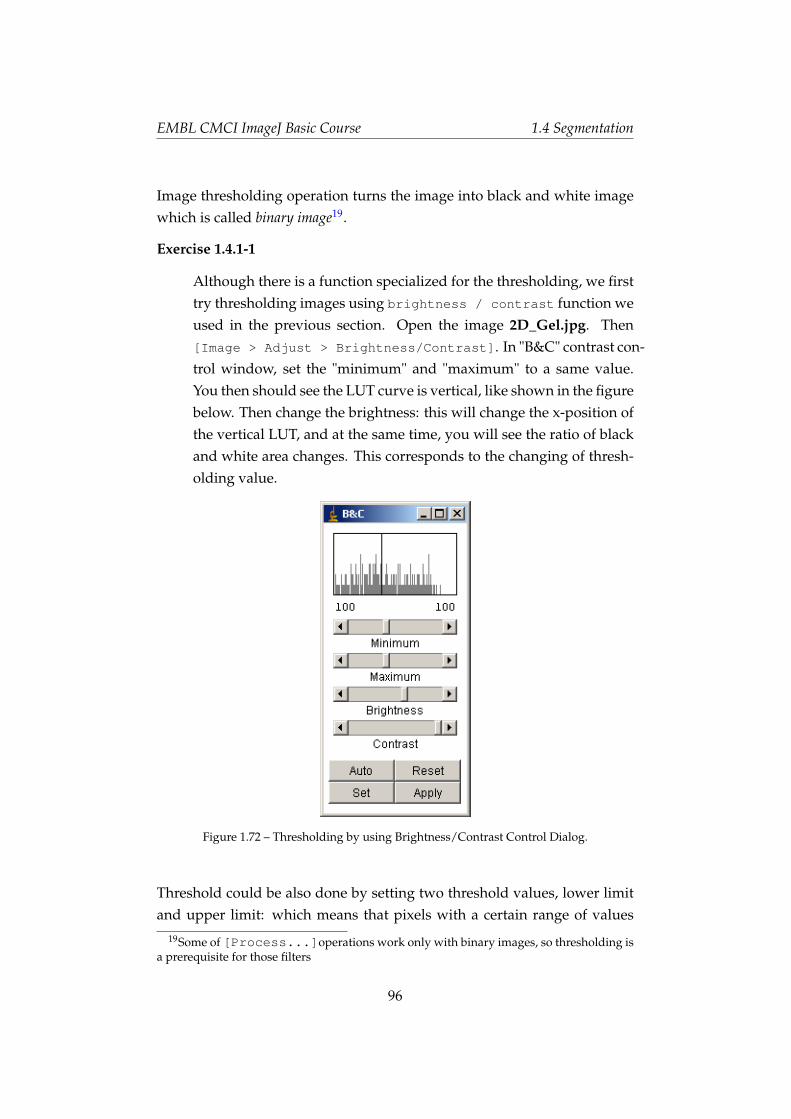
EMBL CMCI ImageJ Basic Course 1.4 Segmentation
Image thresholding operation turns the image into black and white imagewhich is called binary image19.
Exercise 1.4.1-1
Although there is a function specialized for the thresholding, we firsttry thresholding images using brightness / contrast function weused in the previous section. Open the image 2D_Gel.jpg. Then[Image > Adjust > Brightness/Contrast]. In "B&C" contrast con-trol window, set the "minimum" and "maximum" to a same value.You then should see the LUT curve is vertical, like shown in the figurebelow. Then change the brightness: this will change the x-position ofthe vertical LUT, and at the same time, you will see the ratio of blackand white area changes. This corresponds to the changing of thresh-olding value.
Figure 1.72 – Thresholding by using Brightness/Contrast Control Dialog.
Threshold could be also done by setting two threshold values, lower limitand upper limit: which means that pixels with a certain range of values
19Some of [Process...]operations work only with binary images, so thresholding isa prerequisite for those filters
96
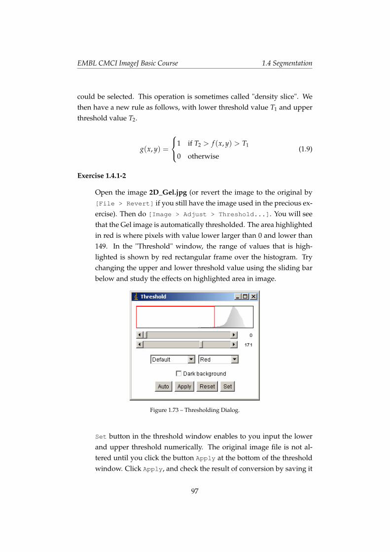
EMBL CMCI ImageJ Basic Course 1.4 Segmentation
could be selected. This operation is sometimes called "density slice". Wethen have a new rule as follows, with lower threshold value T1 and upperthreshold value T2.
g(x, y) =
1 if T2 > f (x, y) > T1
0 otherwise(1.9)
Exercise 1.4.1-2
Open the image 2D_Gel.jpg (or revert the image to the original by[File > Revert] if you still have the image used in the precious ex-ercise). Then do [Image > Adjust > Threshold...]. You will seethat the Gel image is automatically thresholded. The area highlightedin red is where pixels with value lower larger than 0 and lower than149. In the "Threshold" window, the range of values that is high-lighted is shown by red rectangular frame over the histogram. Trychanging the upper and lower threshold value using the sliding barbelow and study the effects on highlighted area in image.
Figure 1.73 – Thresholding Dialog.
Set button in the threshold window enables to you input the lowerand upper threshold numerically. The original image file is not al-tered until you click the button Apply at the bottom of the thresholdwindow. Click Apply, and check the result of conversion by saving it
97

EMBL CMCI ImageJ Basic Course 1.4 Segmentation
as a text file, or simply by checking the pixel values using the valueindicator in the status bar.
Instead of manually setting the threshold level, many algorithms for au-tomatically setting the threshold level exist. Auto button in the thresholdwindow is one of these automatic thresholding algorithms. Various algo-rithms for automatic determination of threshold value are available (suchas Otsu, Maximum Entropy and so on) and you could choose one of themby drop-down menu on the left side. Following is a list of available Algo-rithms:
• IsoData
• Maximum Entropy
• Otsu
• Mixture Modeling
• Huang
• Intermodes
• Li
• Mean
• MinError
• Minimum
• Moments
• Percentile
• RenyiEntropy
• Shanbhag
• Triangle
• Yen
98
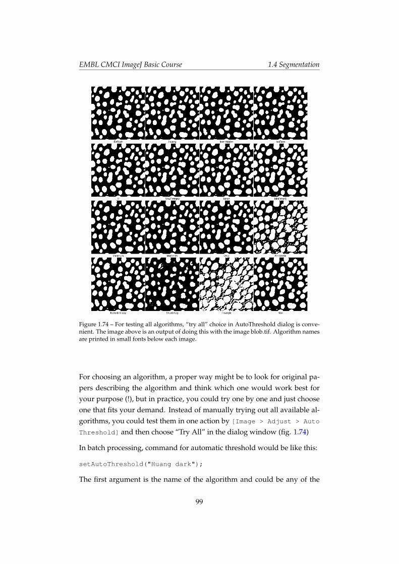
EMBL CMCI ImageJ Basic Course 1.4 Segmentation
Figure 1.74 – For testing all algorithms, “try all” choice in AutoThreshold dialog is conve-nient. The image above is an output of doing this with the image blob.tif. Algorithm namesare printed in small fonts below each image.
For choosing an algorithm, a proper way might be to look for original pa-pers describing the algorithm and think which one would work best foryour purpose (!), but in practice, you could try one by one and just chooseone that fits your demand. Instead of manually trying out all available al-gorithms, you could test them in one action by [Image > Adjust > Auto
Threshold] and then choose “Try All” in the dialog window (fig. 1.74)
In batch processing, command for automatic threshold would be like this:
setAutoThreshold("Huang dark");
The first argument is the name of the algorithm and could be any of the
99
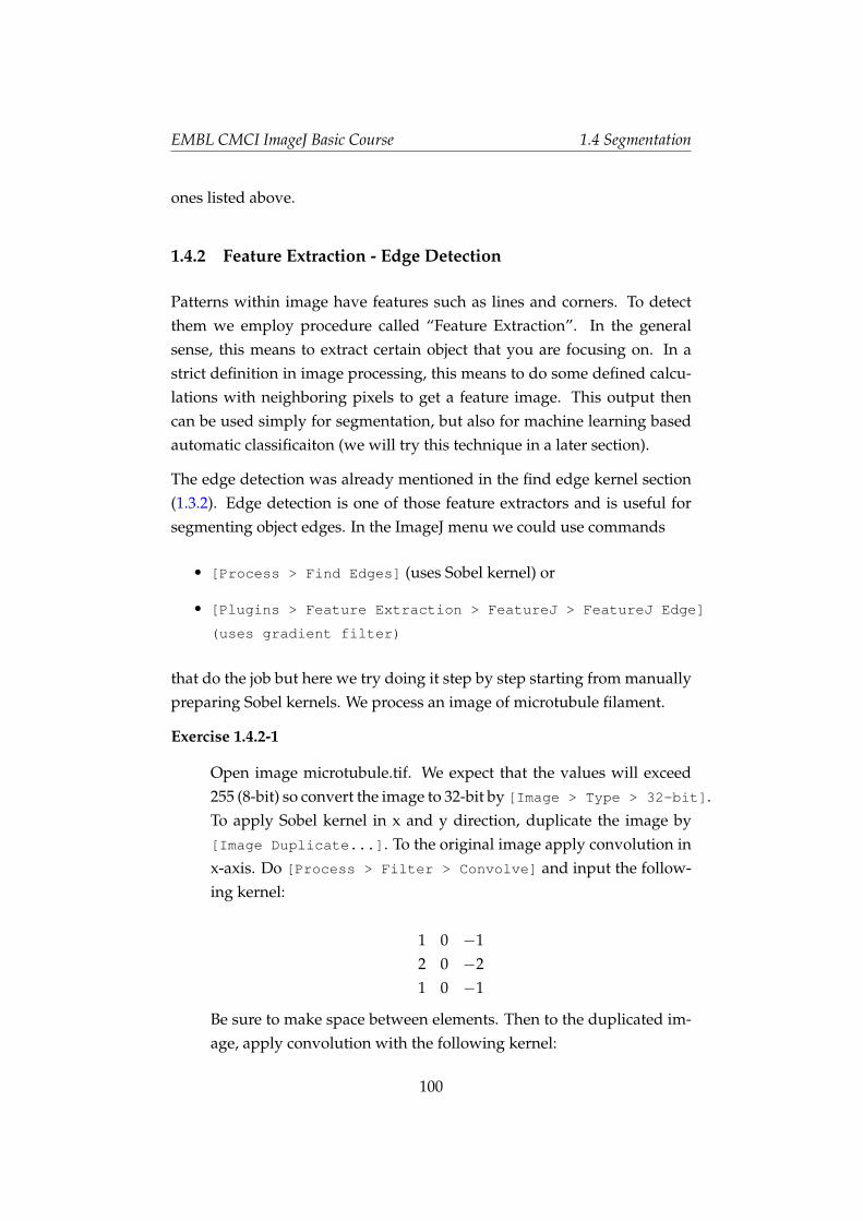
EMBL CMCI ImageJ Basic Course 1.4 Segmentation
ones listed above.
1.4.2 Feature Extraction - Edge Detection
Patterns within image have features such as lines and corners. To detectthem we employ procedure called “Feature Extraction”. In the generalsense, this means to extract certain object that you are focusing on. In astrict definition in image processing, this means to do some defined calcu-lations with neighboring pixels to get a feature image. This output thencan be used simply for segmentation, but also for machine learning basedautomatic classificaiton (we will try this technique in a later section).
The edge detection was already mentioned in the find edge kernel section(1.3.2). Edge detection is one of those feature extractors and is useful forsegmenting object edges. In the ImageJ menu we could use commands
• [Process > Find Edges] (uses Sobel kernel) or
• [Plugins > Feature Extraction > FeatureJ > FeatureJ Edge]
(uses gradient filter)
that do the job but here we try doing it step by step starting from manuallypreparing Sobel kernels. We process an image of microtubule filament.
Exercise 1.4.2-1
Open image microtubule.tif. We expect that the values will exceed255 (8-bit) so convert the image to 32-bit by [Image > Type > 32-bit].To apply Sobel kernel in x and y direction, duplicate the image by[Image Duplicate...]. To the original image apply convolution inx-axis. Do [Process > Filter > Convolve] and input the follow-ing kernel:
1 0 −12 0 −21 0 −1
Be sure to make space between elements. Then to the duplicated im-age, apply convolution with the following kernel:
100
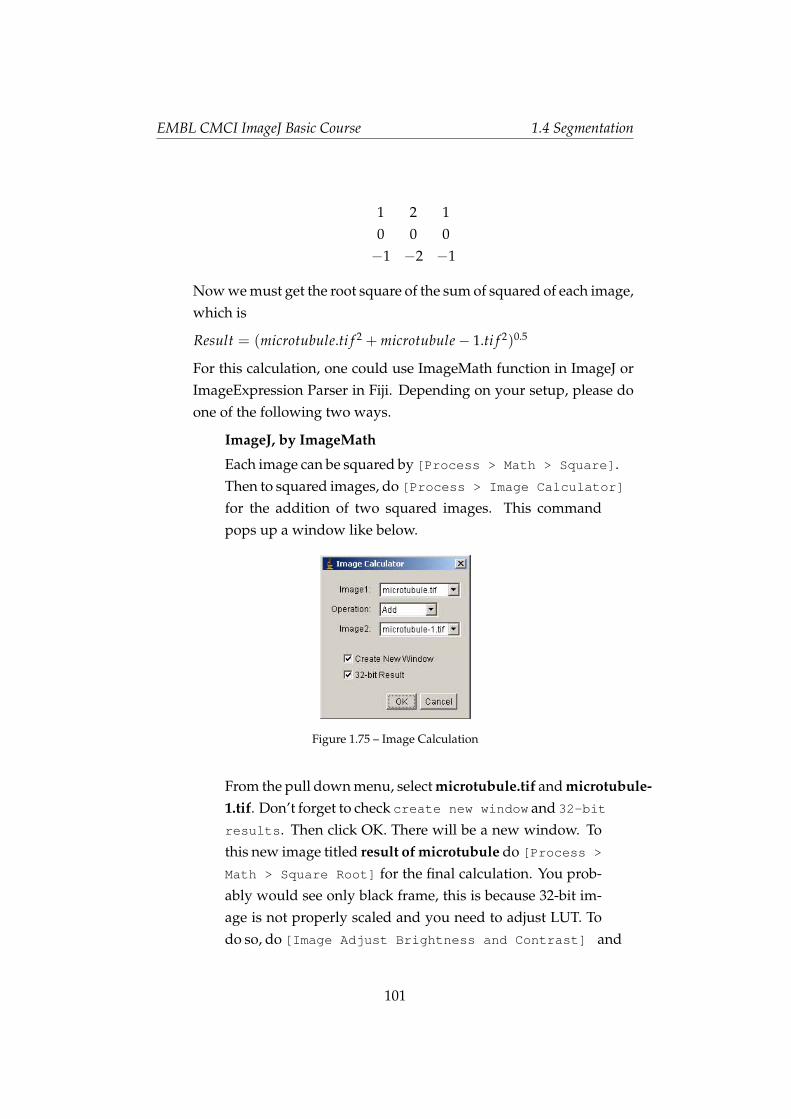
EMBL CMCI ImageJ Basic Course 1.4 Segmentation
1 2 10 0 0−1 −2 −1
Now we must get the root square of the sum of squared of each image,which is
Result = (microtubule.ti f 2 + microtubule− 1.ti f 2)0.5
For this calculation, one could use ImageMath function in ImageJ orImageExpression Parser in Fiji. Depending on your setup, please doone of the following two ways.
ImageJ, by ImageMath
Each image can be squared by [Process > Math > Square].Then to squared images, do [Process > Image Calculator]
for the addition of two squared images. This commandpops up a window like below.
Figure 1.75 – Image Calculation
From the pull down menu, select microtubule.tif and microtubule-1.tif. Don’t forget to check create new window and 32-bit
results. Then click OK. There will be a new window. Tothis new image titled result of microtubule do [Process >
Math > Square Root] for the final calculation. You prob-ably would see only black frame, this is because 32-bit im-age is not properly scaled and you need to adjust LUT. Todo so, do [Image Adjust Brightness and Contrast] and
101
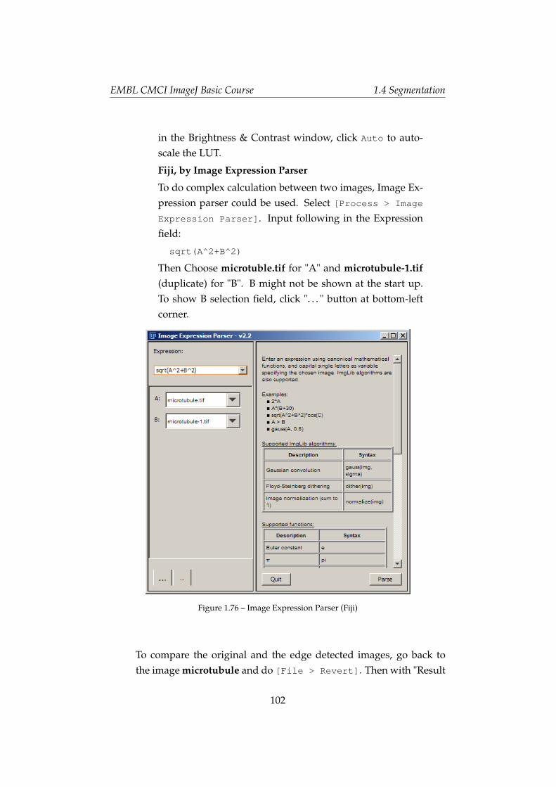
EMBL CMCI ImageJ Basic Course 1.4 Segmentation
in the Brightness & Contrast window, click Auto to auto-scale the LUT.
Fiji, by Image Expression Parser
To do complex calculation between two images, Image Ex-pression parser could be used. Select [Process > Image
Expression Parser]. Input following in the Expressionfield:
sqrt(A^2+B^2)
Then Choose microtuble.tif for "A" and microtubule-1.tif(duplicate) for "B". B might not be shown at the start up.To show B selection field, click ". . . " button at bottom-leftcorner.
Figure 1.76 – Image Expression Parser (Fiji)
To compare the original and the edge detected images, go back tothe image microtubule and do [File > Revert]. Then with "Result
102
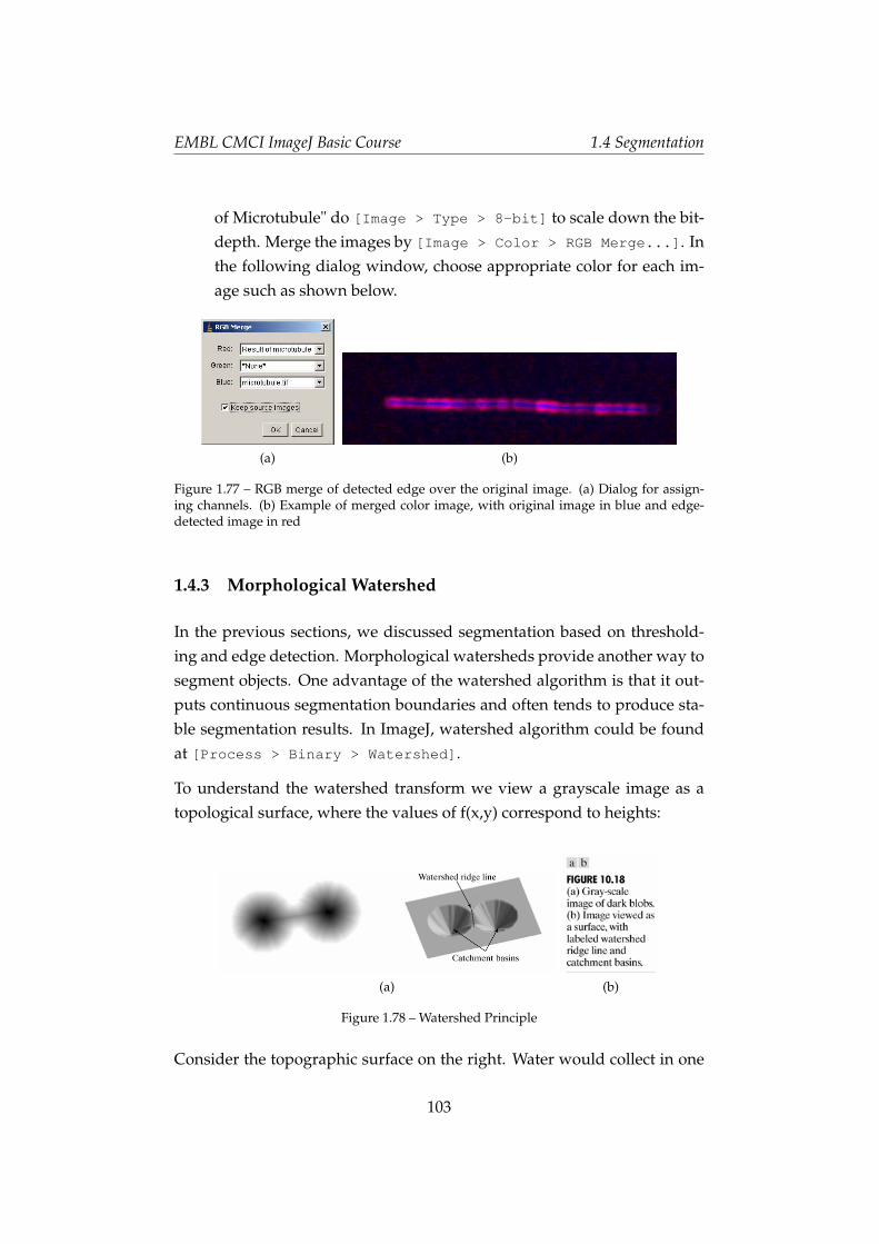
EMBL CMCI ImageJ Basic Course 1.4 Segmentation
of Microtubule" do [Image > Type > 8-bit] to scale down the bit-depth. Merge the images by [Image > Color > RGB Merge...]. Inthe following dialog window, choose appropriate color for each im-age such as shown below.
(a) (b)
Figure 1.77 – RGB merge of detected edge over the original image. (a) Dialog for assign-ing channels. (b) Example of merged color image, with original image in blue and edge-detected image in red
1.4.3 Morphological Watershed
In the previous sections, we discussed segmentation based on threshold-ing and edge detection. Morphological watersheds provide another way tosegment objects. One advantage of the watershed algorithm is that it out-puts continuous segmentation boundaries and often tends to produce sta-ble segmentation results. In ImageJ, watershed algorithm could be foundat [Process > Binary > Watershed].
To understand the watershed transform we view a grayscale image as atopological surface, where the values of f(x,y) correspond to heights:
(a) (b)
Figure 1.78 – Watershed Principle
Consider the topographic surface on the right. Water would collect in one
103
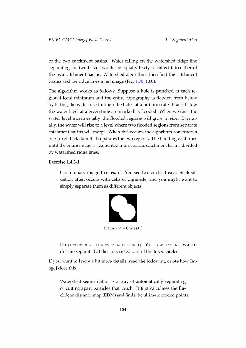
EMBL CMCI ImageJ Basic Course 1.4 Segmentation
of the two catchment basins. Water falling on the watershed ridge lineseparating the two basins would be equally likely to collect into either ofthe two catchment basins. Watershed algorithms then find the catchmentbasins and the ridge lines in an image (Fig. 1.78, 1.80).
The algorithm works as follows: Suppose a hole is punched at each re-gional local minimum and the entire topography is flooded from belowby letting the water rise through the holes at a uniform rate. Pixels belowthe water level at a given time are marked as flooded. When we raise thewater level incrementally, the flooded regions will grow in size. Eventu-ally, the water will rise to a level where two flooded regions from separatecatchment basins will merge. When this occurs, the algorithm constructs aone-pixel thick dam that separates the two regions. The flooding continuesuntil the entire image is segmented into separate catchment basins dividedby watershed ridge lines.
Exercise 1.4.3-1
Open binary image Circles.tif. You see two circles fused. Such sit-uation often occurs with cells or organelle, and you might want tosimply separate them as different objects.
Figure 1.79 – Circles.tif
Do [Process > Binary > Watershed]. You now see that two cir-cles are separated at the constricted part of the fused circles.
If you want to know a bit more details, read the following quote how Im-ageJ does this.
Watershed segmentation is a way of automatically separatingor cutting apart particles that touch. It first calculates the Eu-clidean distance map (EDM) and finds the ultimate eroded points
104
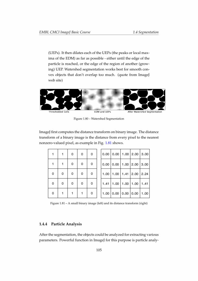
EMBL CMCI ImageJ Basic Course 1.4 Segmentation
(UEPs). It then dilates each of the UEPs (the peaks or local max-ima of the EDM) as far as possible - either until the edge of theparticle is reached, or the edge of the region of another (grow-ing) UEP. Watershed segmentation works best for smooth con-vex objects that don’t overlap too much. (quote from ImageJweb site)
Figure 1.80 – Watershed Segmentation
ImageJ first computes the distance transform on binary image. The distancetransform of a binary image is the distance from every pixel to the nearestnonzero-valued pixel, as example in Fig. 1.81 shows.
Figure 1.81 – A small binary image (left) and its distance transform (right)
1.4.4 Particle Analysis
After the segmentation, the objects could be analyzed for extracting variousparameters. Powerful function in ImageJ for this purpose is particle analy-
105
EMBL CMCI ImageJ Basic Course 1.4 Segmentation
sis function. It counts the number of objects (particles) in the image, extractmorphological parameters, measures intensity. . . and so on. For details onextractable parameters, refer to Appendix 1.6.4 of this textbook. Here, wetake an example to learn the basic use of this function.
Exercise 1.4.4-1
Single Particle Detection
Load Circles.tif and segment two circles by watershed operation as
we did in the previous section. Then select the Wand Tool fromthe tool bar. Click one of the circles. Check that a ROI is automaticallycreated at the edge of the circle.
Automatic detection is done by pixel similarity principle. In the above caseusing the wand tool, computer searches for pixels in the surrounding of theclicked pixel for similarity in the pixel value. Similar pixels will be labeled.Then in the next round, computer searches for each of the labeled pixelfor similar surrounding. This continues until searching hits the boundary.Particle analysis uses the same strategy, but there will be specific labelingfor each particle.
Exercise 1.4.4-2
Multiple Particle Analysis: Open rice.tif. Before applying particleanalysis, target particles must be segmented by image threshold. Trythresholding the image. . . What you would find out immediately isthat there is shading in the image that rice can not be uniformly se-lected by thresholded. For this reason, do the background subtractionas we already did in 1.3.5. We then work with the subtracted imagein the following.
Set Threshold again, and then click “Apply” in the Threshold dialogwindow. The image then should be black and white. This binarized(segmented) image will be used as a reference for setting boundaryof each rice grain.
Open file rice.tif again. Since there is already a window with sametitle, this second one should have a title “rice-1.tif”. By having thisoriginal image, boundary that will be set using binarized image will
106
EMBL CMCI ImageJ Basic Course 1.4 Segmentation
be "redirected" when measurement is actually taking place20.
Before doing particle analysis, you must specify what you want tomeasure for each particle through [Analysis > Set Measurements].Select Area, Circularity, Centroid and Perimeter (details on these pa-rameters are written in Appendix 1.6.4). In addition, set “redirect to”to the original image (rice-1.tif) so that the measurement will be donewith the original image and not with the thresholded image.
Activate the threshold the image, and then do [Analyze Analyze
Particles...]. A dialog window pops up. Input following param-eters:
• Size: "0-200" size above 200 pixel area will be excluded from themeasurement
• Circularity: use default "0-1.0"
• Show: Outline
• Check box:
– Check "Display Results" to display the result table.
– Check "Clear Results" to refresh the measurement record-ings.
– Check "Exclude on Edges" to exclude particles touching theedge of the image.
Then Click "OK". Two windows pop up. One is the outline imageof the measured particles, with number labels. These numbers cor-respond to the numbers you see at the left most column in the resultwindow, which also popped up. Examine the outline image. At thebottom, there seems to be some particles which are counted but onlypart of the particles are included.
20It is also possible to do the measurement without redirecting: for example, you couldsimply image-threshold, and while the image is highlighted with red, (do not click Applybutton) and do “Analyze particle”. This will then detect particles which are highlighted.
107
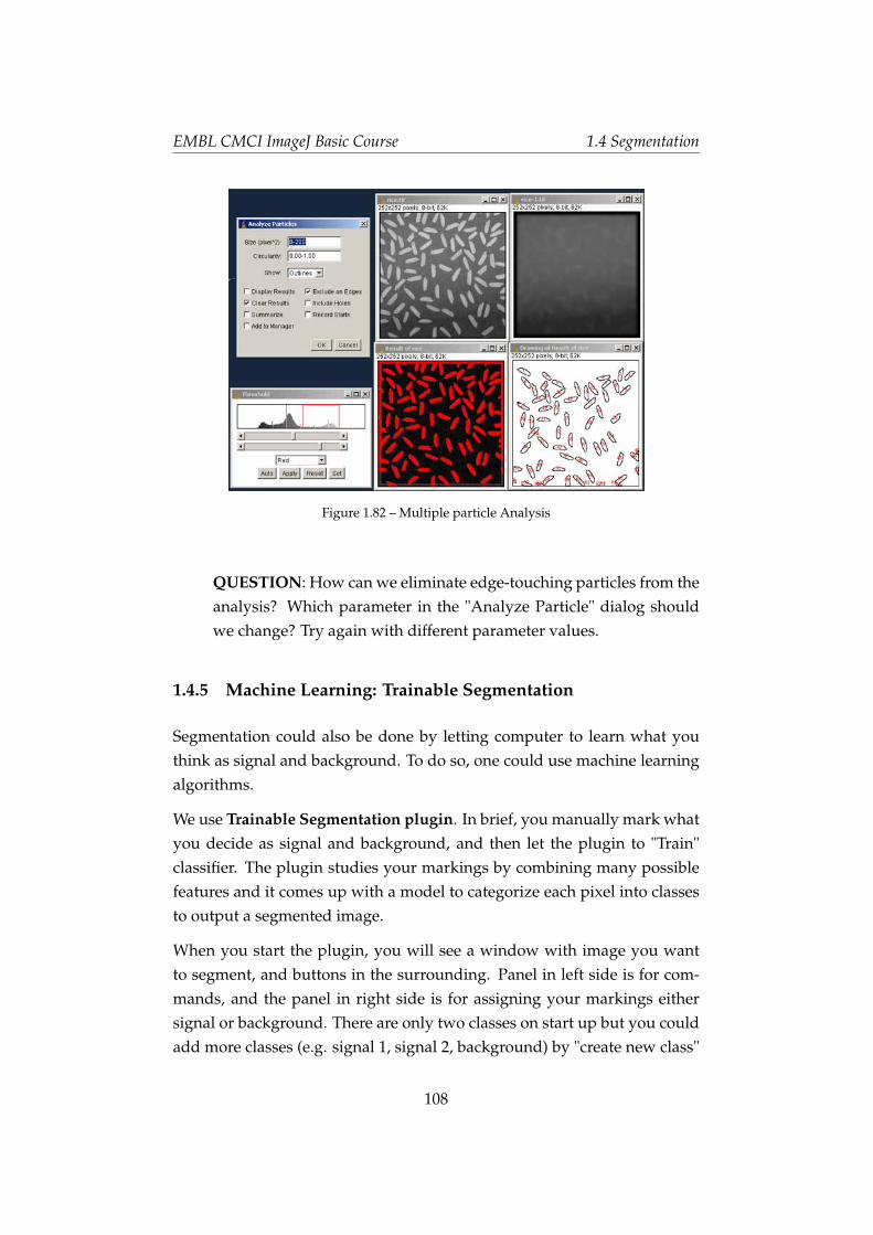
EMBL CMCI ImageJ Basic Course 1.4 Segmentation
Figure 1.82 – Multiple particle Analysis
QUESTION: How can we eliminate edge-touching particles from theanalysis? Which parameter in the "Analyze Particle" dialog shouldwe change? Try again with different parameter values.
1.4.5 Machine Learning: Trainable Segmentation
Segmentation could also be done by letting computer to learn what youthink as signal and background. To do so, one could use machine learningalgorithms.
We use Trainable Segmentation plugin. In brief, you manually mark whatyou decide as signal and background, and then let the plugin to "Train"classifier. The plugin studies your markings by combining many possiblefeatures and it comes up with a model to categorize each pixel into classesto output a segmented image.
When you start the plugin, you will see a window with image you wantto segment, and buttons in the surrounding. Panel in left side is for com-mands, and the panel in right side is for assigning your markings eithersignal or background. There are only two classes on start up but you couldadd more classes (e.g. signal 1, signal 2, background) by "create new class"
108
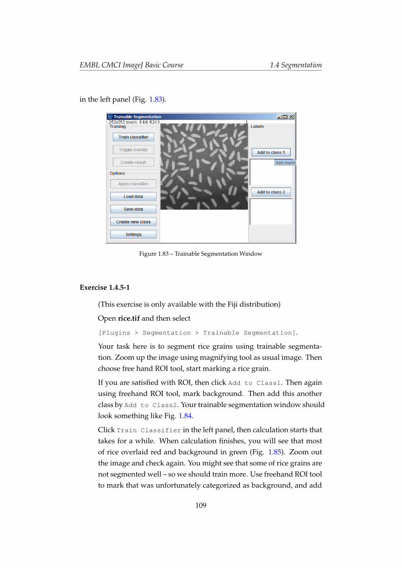
EMBL CMCI ImageJ Basic Course 1.4 Segmentation
in the left panel (Fig. 1.83).
Figure 1.83 – Trainable Segmentation Window
Exercise 1.4.5-1
(This exercise is only available with the Fiji distribution)
Open rice.tif and then select
[Plugins > Segmentation > Trainable Segmentation].
Your task here is to segment rice grains using trainable segmenta-tion. Zoom up the image using magnifying tool as usual image. Thenchoose free hand ROI tool, start marking a rice grain.
If you are satisfied with ROI, then click Add to Class1. Then againusing freehand ROI tool, mark background. Then add this anotherclass by Add to Class2. Your trainable segmentation window shouldlook something like Fig. 1.84.
Click Train Classifier in the left panel, then calculation starts thattakes for a while. When calculation finishes, you will see that mostof rice overlaid red and background in green (Fig. 1.85). Zoom outthe image and check again. You might see that some of rice grains arenot segmented well – so we should train more. Use freehand ROI toolto mark that was unfortunately categorized as background, and add
109
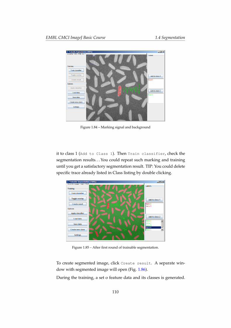
EMBL CMCI ImageJ Basic Course 1.4 Segmentation
Figure 1.84 – Marking signal and background
it to class 1 (Add to Class 1). Then Train classifier, check thesegmentation results. . . You could repeat such marking and traininguntil you get a satisfactory segmentation result. TIP: You could deletespecific trace already listed in Class listing by double clicking.
Figure 1.85 – After first round of trainable segmentation.
To create segmented image, click Create result. A separate win-dow with segmented image will open (Fig. 1.86).
During the training, a set o feature data and its classes is generated.
110
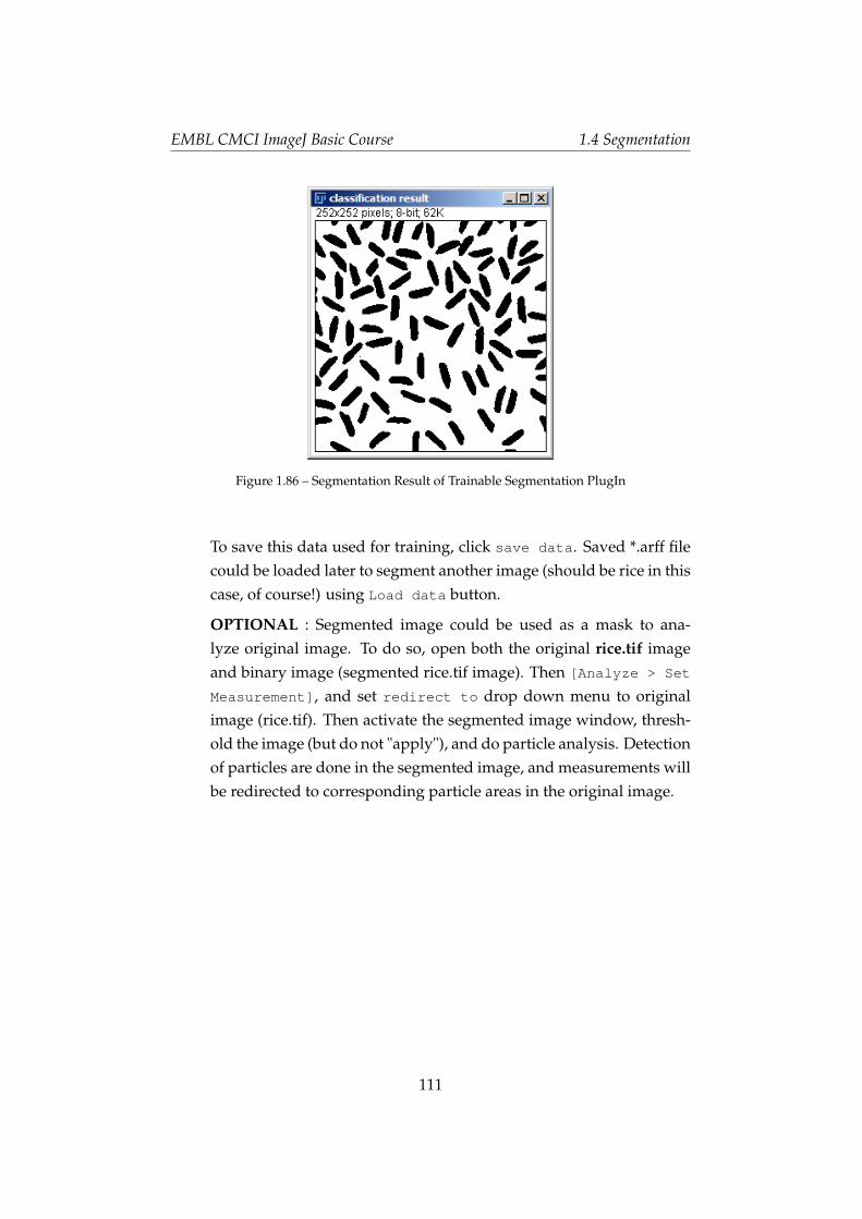
EMBL CMCI ImageJ Basic Course 1.4 Segmentation
Figure 1.86 – Segmentation Result of Trainable Segmentation PlugIn
To save this data used for training, click save data. Saved *.arff filecould be loaded later to segment another image (should be rice in thiscase, of course!) using Load data button.
OPTIONAL : Segmented image could be used as a mask to ana-lyze original image. To do so, open both the original rice.tif imageand binary image (segmented rice.tif image). Then [Analyze > Set
Measurement], and set redirect to drop down menu to originalimage (rice.tif). Then activate the segmented image window, thresh-old the image (but do not "apply"), and do particle analysis. Detectionof particles are done in the segmented image, and measurements willbe redirected to corresponding particle areas in the original image.
111
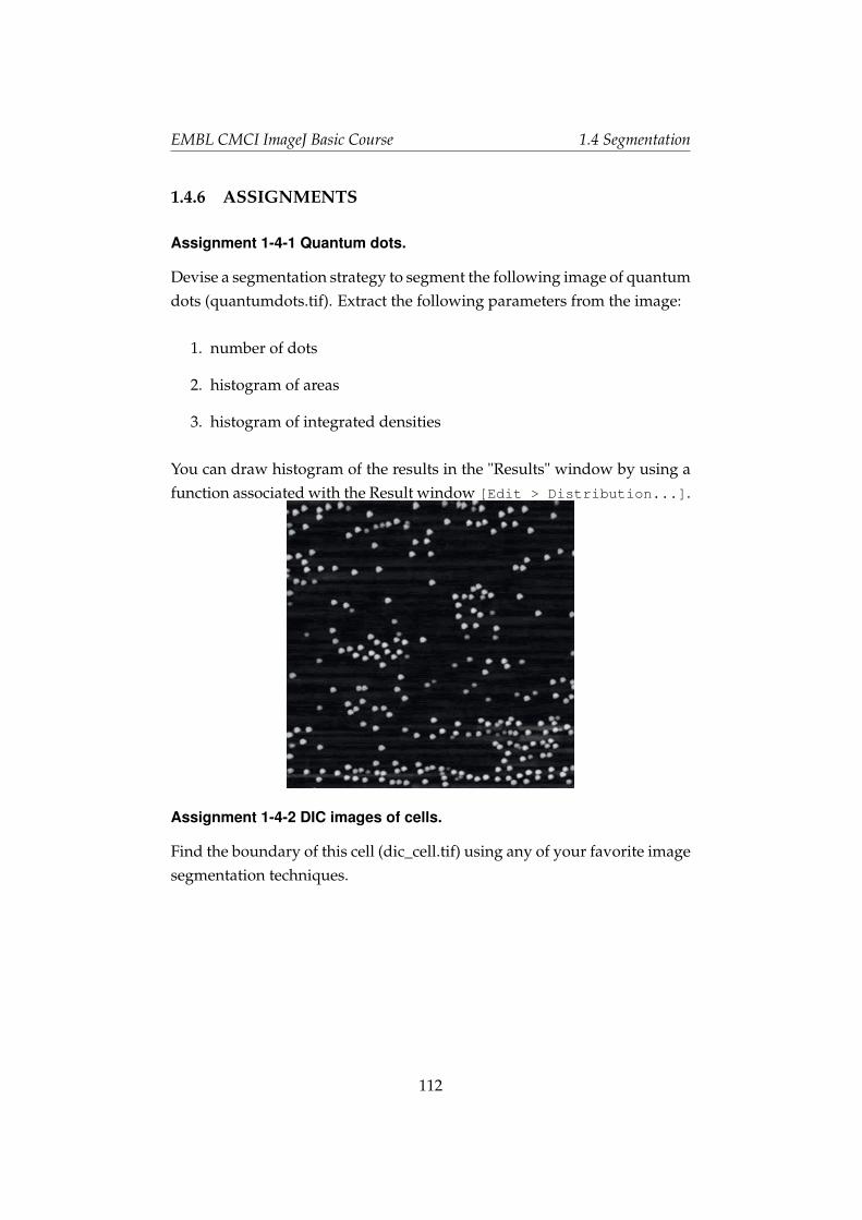
EMBL CMCI ImageJ Basic Course 1.4 Segmentation
1.4.6 ASSIGNMENTS
Assignment 1-4-1 Quantum dots.
Devise a segmentation strategy to segment the following image of quantumdots (quantumdots.tif). Extract the following parameters from the image:
1. number of dots
2. histogram of areas
3. histogram of integrated densities
You can draw histogram of the results in the "Results" window by using afunction associated with the Result window [Edit > Distribution...].
Assignment 1-4-2 DIC images of cells.
Find the boundary of this cell (dic_cell.tif) using any of your favorite imagesegmentation techniques.
112
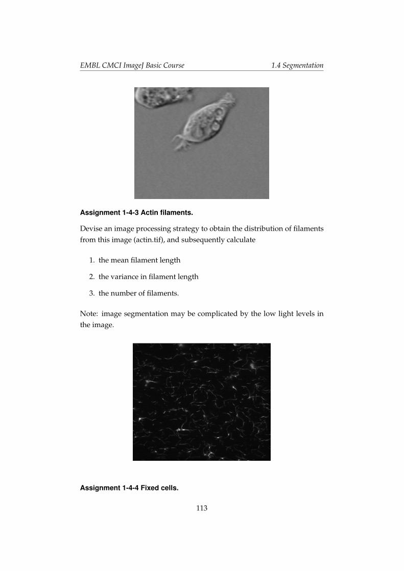
EMBL CMCI ImageJ Basic Course 1.4 Segmentation
Assignment 1-4-3 Actin filaments.
Devise an image processing strategy to obtain the distribution of filamentsfrom this image (actin.tif), and subsequently calculate
1. the mean filament length
2. the variance in filament length
3. the number of filaments.
Note: image segmentation may be complicated by the low light levels inthe image.
Assignment 1-4-4 Fixed cells.
113
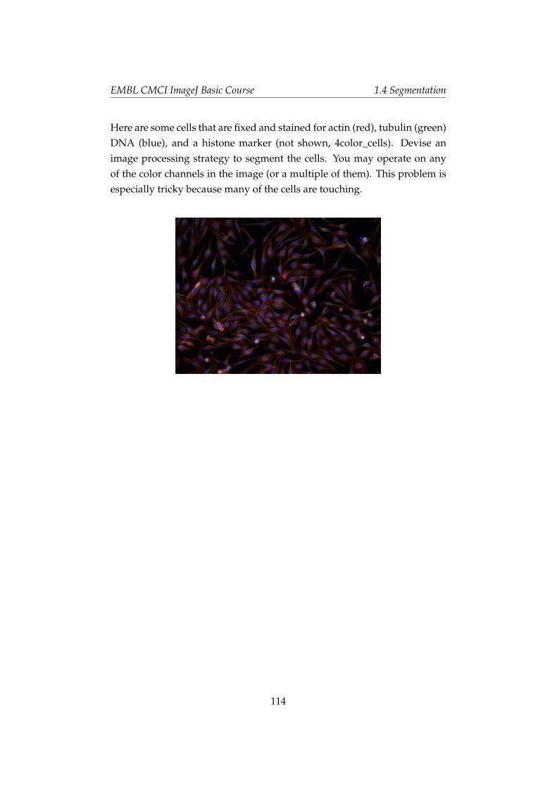
EMBL CMCI ImageJ Basic Course 1.4 Segmentation
Here are some cells that are fixed and stained for actin (red), tubulin (green)DNA (blue), and a histone marker (not shown, 4color_cells). Devise animage processing strategy to segment the cells. You may operate on anyof the color channels in the image (or a multiple of them). This problem isespecially tricky because many of the cells are touching.
114
EMBL CMCI ImageJ Basic Course 1.5 Analysis of Time Series
1.5 Analysis of Time Series
In this section, we learn how to analyze dynamics using image sequences.A time series of digital images, usually called "stack", contains temporaldynamics of position and intensity, and kinetics can be obtained from thesedata21. In general there are three types of dynamics.
1. Position does not change but intensity changes over time.
2. Position changes but the intensity does not change.
3. Both Position and Intensity change over time.
An example of type (1) is the measurement of cargo transport dynamicsin vesicle trafficking (Hirschberg et al., 1998). Transition of protein local-ization from ER to Golgi then to the plasma membrane was measuredover time by measuring the signal intensity in each statically positionedcompartment. This type of technique has evolved to various sophisticatedmethods based on the same principle -measurement of signal intensity at aconstant position. Type (2) corresponds to the measurement of movement,or object tracking, and an example is the single particle tracking of mem-brane surface proteins (Murase et al., 2004). An example of type (3) mea-surement is the measurement of chemotaxis-related protein accumulationdynamics during the Dictyostelium cell migration (Dormann et al., 2002).Analysis of type (3) dynamics is more specific and advanced, so refer toother literature (Miura, 2005).
1.5.1 Difference Images
In some cases, mathematical operations on image sequences is effectivein visualizing dynamics. "Difference images" (also called "subtraction im-ages") is one of such techniques. A difference image of successive framesin a sequence is given by:
Dj(x, y) = Ij+1(x, y)− Ij(x, y) (1.10)
21For basics to deal with stack, go to 1.1.9
115
EMBL CMCI ImageJ Basic Course 1.5 Analysis of Time Series
where D is the difference image, and j is a given plane in the stack. Differ-ence images highlight features of the image that change rapidly over time,much in the same way that a spatial gradient enhances contrast around anedge. The change is usually brought about by movement of an object inthe image, or by a kinetic process that has not reached steady-state (likephotobleaching).
Exercise 1.5.1-1
Open image stack 1703-2(3s-20s).stk. Then duplicate the stack [Edit
> Duplicate]. Don’t forget checking the "Duplicate entire stack".Go back to the original stack, delete the last frame (frame 31) [Image> Stacks >Delete Slice]. Alternatively, you could simply click "-" button in the stack tools at the last frame. Activate the duplicatedstack and delete the first frame. Then do subtraction [Process >
Image > Calculator]:
OriginalStack− DupicatedStack
This will then subtract frame 1 – frame2, frame2 – frame 3 . . . and soon. Do you see Frapped Region in the difference image stack?
1.5.2 Projection of Time Series
A maximum intensity projection of an entire image stack is given by
M(x, y) = maxj(Ij(x, y)) (1.11)
The maximum on the right hand side is the maximum in intensity valueat a given pixel position over all time frames in an image. Maximum pro-jections collapse the entire dynamics of the stack onto a single plane. Thisfunction is especially useful for visualizing entire trajectories of movingparticles on a single plane. Additional merit is that this operation discardsnoise within the sequence.
Exercise 1.5.2-1
Open image listeriacells.stk. Then do all types of projections youcould choose by [Image > Stack > Z projection...].
116

EMBL CMCI ImageJ Basic Course 1.5 Analysis of Time Series
Question: Which is the best method for leaving the bacteria tracks?
1.5.3 Measurement of Intensity dynamics
Temporal changes in fluorescence level matters a lot in biological exper-iments since the change is directly related to the molecular mobility andproduction. Here, we study how to obtain the intensity dynamics out ofimage sequences.
Exercise 1.5.3-1
Load image stack 1703-2(3s-20s).stk. This is a sequence of FRAPexperiment. Draw a ROI (could be any closed ROI) surroundingthe area where the photobleaching takes place. Then do [Image >
Stacks > Plot z-axis Profile].
There will be two windows: "Results" window and a graph of inten-sity dynamics.
Try adding Second ROI to measure the background, simply by mak-ing another ROI. So the intensity measurement again with this newROI.
OPTIONAL: Numerical values in the table can be copy and pastedin spread sheet software like Excel or OpenOffice Calc. If you knowhow to use R, then you could save the results table as a CSV file andread it from R. Try draw a graph in your favorite plotting software.
When you measure the fluorescence level, it is very important to measurethe background intensity and subtract the value from the measured flu-orescence. This is because the baseline level adds offset to the measuredvalue, so you could not quantify the true value.
1.5.4 Measurement of Movement Dynamics
Movement is an essential component of biological system. To quantify themovement dynamics, various methods has been developed. In case of im-age sequences, particle tracking is a popular way to quantify movement(1.5.6, 1.5.7). In any tracking methods, the ultimate goal is to obtain the po-
117
EMBL CMCI ImageJ Basic Course 1.5 Analysis of Time Series
sition coordinate of a target object in each image frame, so that the move-ment of the target object can be represented as changes in the position co-ordinate. Velocity and movement direction can then be calculated fromthe resulting coordinate series. Since tracking deals with segmentation andposition linking, the process is rather complex. Besides tracking, there is aeasier way to represent and quantify movements occurring in sequences.The technique is called "kymographs (1.5.5: see below)". This method losespositional information but for measuring velocity, the method is easy andfast.The process of tracking has two major steps. In the first step the object mustbe segmented. This then enables us to calculate the coordinate of the objectposition, such as its centroid. There are various ways to do segmentation(see 1.4). In the second step the successive positions of the object must belinked to obtain a series of coordinates of that object. We call this process"position linking". Position linking becomes difficult when there are toomany similar objects. In this case it would become impossible to identifythe object in the next time point among multiple candidates. Position link-ing also becomes difficult when the successive positions of the object aretoo far apart. This happens when the time interval between frames is toolong. In this case, multiple candidates may appear in the next time pointeven though similar objects are only sparsely present in the image frame. Ifthe target object is single and unique, linking of coordinates to successivetime points has none of these problems.
1.5.5 Kymographs
Kymographs are a two-dimensional time traces, where time t is in Y axisand space along a one-dimensional contour is in X, and the dynamical vari-able F(x,t) is visualized as an image. Kymographs provide a fast and con-venient way to visualize motion and dynamics in microscopy images.
Exercise 1.5.5-1
We try measuring the speed of tubulin flux using Kymographs. Fordoing this exercise, you need "Slice Remover" PlugIn 22.
22To install the plugin refer to 1.6.2. If you are using Fiji, Slice Remover is already in-stalled. Access the command by [Image > Stack > Manipulation > Slice
118
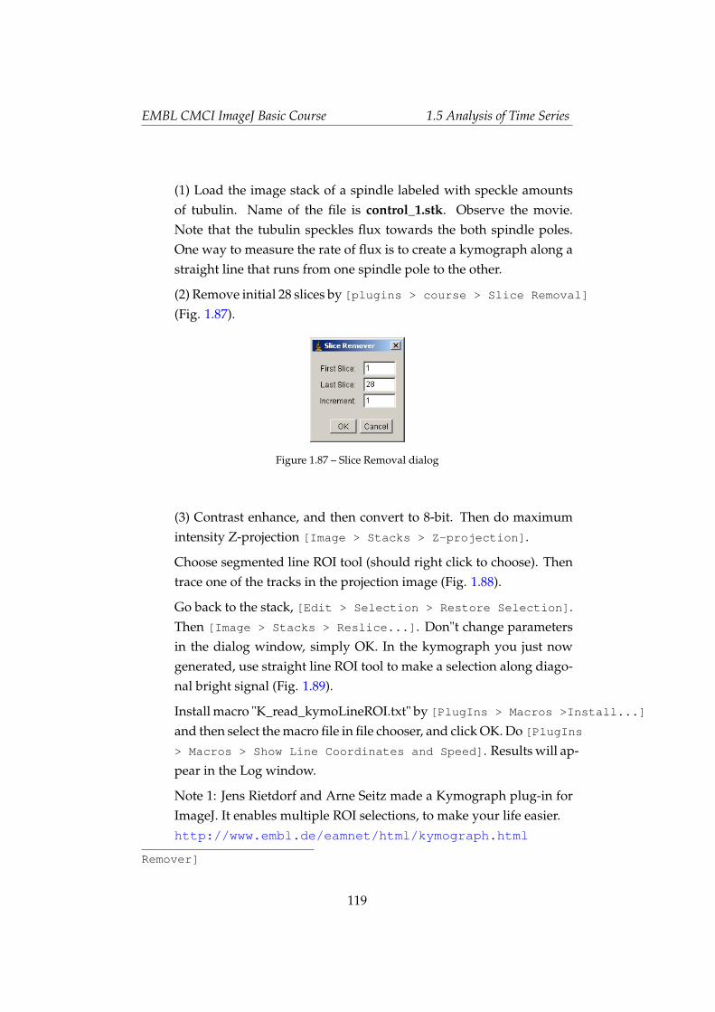
EMBL CMCI ImageJ Basic Course 1.5 Analysis of Time Series
(1) Load the image stack of a spindle labeled with speckle amountsof tubulin. Name of the file is control_1.stk. Observe the movie.Note that the tubulin speckles flux towards the both spindle poles.One way to measure the rate of flux is to create a kymograph along astraight line that runs from one spindle pole to the other.
(2) Remove initial 28 slices by [plugins > course > Slice Removal]
(Fig. 1.87).
Figure 1.87 – Slice Removal dialog
(3) Contrast enhance, and then convert to 8-bit. Then do maximumintensity Z-projection [Image > Stacks > Z-projection].
Choose segmented line ROI tool (should right click to choose). Thentrace one of the tracks in the projection image (Fig. 1.88).
Go back to the stack, [Edit > Selection > Restore Selection].Then [Image > Stacks > Reslice...]. Don"t change parametersin the dialog window, simply OK. In the kymograph you just nowgenerated, use straight line ROI tool to make a selection along diago-nal bright signal (Fig. 1.89).
Install macro "K_read_kymoLineROI.txt" by [PlugIns > Macros >Install...]
and then select the macro file in file chooser, and click OK. Do [PlugIns> Macros > Show Line Coordinates and Speed]. Results will ap-pear in the Log window.
Note 1: Jens Rietdorf and Arne Seitz made a Kymograph plug-in forImageJ. It enables multiple ROI selections, to make your life easier.http://www.embl.de/eamnet/html/kymograph.html
Remover]
119
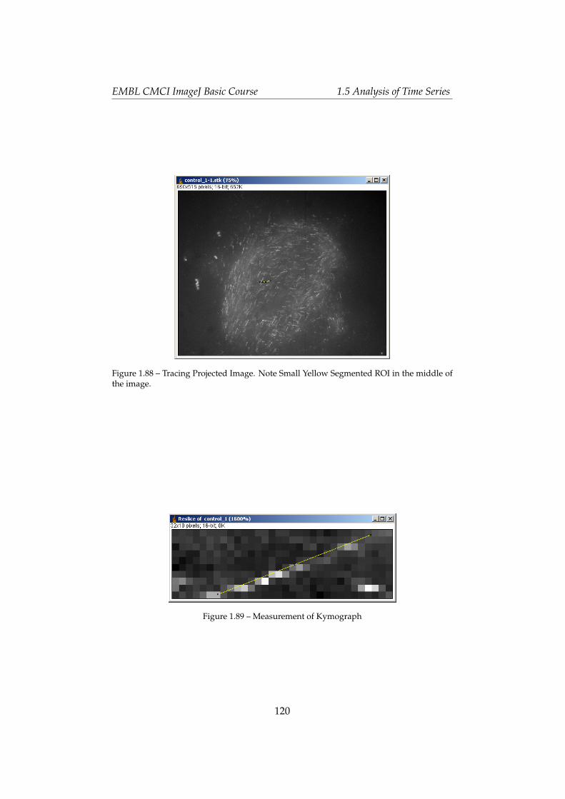
EMBL CMCI ImageJ Basic Course 1.5 Analysis of Time Series
Figure 1.88 – Tracing Projected Image. Note Small Yellow Segmented ROI in the middle ofthe image.
Figure 1.89 – Measurement of Kymograph
120
EMBL CMCI ImageJ Basic Course 1.5 Analysis of Time Series
Note 2: If you want to quantify kymograph with ambiguous patterns,you could try using “kymoquant”, an ImageJ macro. For more de-tails, see http://cmci.embl.de/downloads/kymoquant
1.5.6 Manual Tracking
In the simplest case, tracking can be done manually. The user can read outthe coordinate position of the target object directly from the imaging soft-ware. In ImageJ, user can read out position coordinate indicated in the sta-tus bar by placing the cross-hair pointer over the object. Then coordinatescan be listed in standard spreadsheet software such as Microsoft Excel forfurther analysis.
An ImageJ plug-in is also freely available to assist such simple way of track-ing. An obvious disadvantage of the manual tracking is that the mouse-clicking by the user could be erroneous, as we are still human who getstired after thousands of clicking. For such errors, measurement errors canbe estimated by tracking the same object several times and this error couldthen be indicated together with the results. Otherwise, automated trackingis more objective, but if you have only limited number of tracks to analyze,manual tracking is a best choice before start to explore complex parameterspace of automated tracking setting.
The manual tracking can be assisted by an ImageJ plug-in "Manual Track-ing". This plug-in enables the user to record x-y coordinates of the posi-tion where the user clicked using mouse in each frame within a stack. Thedownload site has a detailed instruction on how to use.
http://rsb.info.nih.gov/ij/plugins/track/track.html
Exercise 1.5.6-1
Manual Tracking: In a spindle, microtubules attach to chromosomesthrough structures called kinetochores. In the stack kin.stk, kineto-chores are labeled with a fluorescent marker. Your task now is to trackthe movement of individual kinetochores using the ManualTrackerPlugIn. Enhance contrast and convert the image stack from 16-bit to8-bit (just to decrease the memory load. If your computer is powerful
121
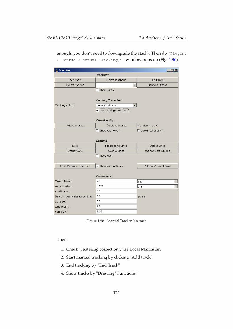
EMBL CMCI ImageJ Basic Course 1.5 Analysis of Time Series
enough, you don’t need to downgrade the stack). Then do [Plugins
> Course > Manual Tracking]: a window pops up (Fig. 1.90).
Figure 1.90 – Manual Tracker Interface
Then
1. Check "centering correction", use Local Maximum.
2. Start manual tracking by clicking "Add track".
3. End tracking by "End Track"
4. Show tracks by "Drawing" Functions"
122
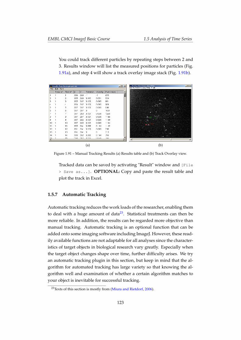
EMBL CMCI ImageJ Basic Course 1.5 Analysis of Time Series
You could track different particles by repeating steps between 2 and3. Results window will list the measured positions for particles (Fig.1.91a), and step 4 will show a track overlay image stack (Fig. 1.91b).
(a) (b)
Figure 1.91 – Manual Tracking Results (a) Results table and (b) Track Overlay view.
Tracked data can be saved by activating "Result" window and [File
> Save as...]. OPTIONAL: Copy and paste the result table andplot the track in Excel.
1.5.7 Automatic Tracking
Automatic tracking reduces the work loads of the researcher, enabling themto deal with a huge amount of data23. Statistical treatments can then bemore reliable. In addition, the results can be regarded more objective thanmanual tracking. Automatic tracking is an optional function that can beadded onto some imaging software including ImageJ. However, these read-ily available functions are not adaptable for all analyses since the character-istics of target objects in biological research vary greatly. Especially whenthe target object changes shape over time, further difficulty arises. We tryan automatic tracking plugin in this section, but keep in mind that the al-gorithm for automated tracking has large variety so that knowing the al-gorithm well and examination of whether a certain algorithm matches toyour object is inevitable for successful tracking.
23Texts of this section is mostly from (Miura and Rietdorf, 2006).
123
EMBL CMCI ImageJ Basic Course 1.5 Analysis of Time Series
In the following, I will list some of the standard methods for the automaticsegmentation of objects, which is the first part of the automated tracking.Detected objects are then linked from a frame to the other.
CentroidMethod
The centroid is the average of all pixel coordinates inside the segmentedobject and is the most commonly used feature for representing the objectposition. The centroid coordinate pc(x, y) can be calculated as
pc(x, y) = (∑ xi
nx, ∑ yi
ny)|x,y∈R (1.12)
where R is the region surrounded by the contour, and n is the total numberof pixels within that region. In other words, all x coordinates of the pixelsinside the object are added and averaged. The same happens for all y co-ordinates. The derived averages for x and y coordinates represent the cen-troid coordinates of the object. The position of the object can be measuredfor every frame of the sequence manually. In ImageJ, centroid calculationis available in the "Particle Analysis" function.
Gaussian Fitting Method
For spherical signals such as fluorescence beads or fluorescently labeledsub-resolution particle, the signal intensity distribution can be fitted to astandard two-dimensional Gaussian curve (Anderson et al., 1992; Schützet al., 1997; Tardin et al., 2003):
I(x, y) = z0 + znexp− (x− Xn)2 + (y−Yn)2
W2n
(1.13)
where I(x, y) is the intensity distribution of an image, z0 is the backgroundintensity, and zn is the height of the peak. Wn is the width of the curve thatpeaks at (Xn, Yn). This peak position is the signal position. Although thisfitting method is restricted to spherical or oval objects, it yields the mostprecise measurements even with a very low signal-to-noise ratio (Cheezum
124
EMBL CMCI ImageJ Basic Course 1.5 Analysis of Time Series
et al., 2001). Another advantage of the Gaussian fitting method is that theresults are in sub-pixel resolution. Such high resolution can for exampleenable the analysis of molecular diffusion in the nm resolution. More dis-cussion on the localization accuracy in the position measurements can befound in the literature (Ober et al., 2004; Martin et al., 2002; Thompson et al.,2002).
Pattern Matching Method
In this method, a kernel containing a template pattern of the object is com-pared to different positions within the image in order to find a position withthe highest similarity to the kernel. A cross-correlation function C(x, y)is usually used to evaluate the resemblance of the template with differentparts of the image, (Gilles et al. 1988):
C(x, y) =n−1
∑i=0
m−1
∑j=0
I(x + i)(y + j)K(i, j)− K (1.14)
where I(x, y) is the intensity distribution of the image frame and K(i, j) is an x m pixels kernel that contains the template image pattern. K is the meanintensity of the kernel. C(x, y) will be maximal at the position where thepattern best matches. In actual application, the template pattern is sampledin the k-th image frame Ik(x, y) by the user manually or by semi-automaticsegmentation. Then the cross-correlation value C(x, y) between this tem-plate kernel and the consecutive k + 1-th image frame Ik+1(x, y) can be cal-culated. Gelles et al. (1988) introduced the following formula for obtainingthe peak position (xc, yc):
Xc =∑ xC(x, y)− T∑ C(x, y)− T (1.15)
yc =∑ yC(x, y)− T∑ C(x, y)− T (1.16)
where T is the threshold value and negative values are discarded. (xc, yc)
corresponds to the centroid of the magnitude of correlation that is thresh-olded by T.
125
EMBL CMCI ImageJ Basic Course 1.5 Analysis of Time Series
Since the cross-correlation function 1.14 tends to give higher values at brighterregions rather than at regions of similar shapes, a normalized form of cross-correlation can also be used:
Cn(x, y) =∑n−1
i=0 ∑m−1j=0 [I(x + i)(y + j)− I]K(i, j)− K
MIx,y ·Mk(1.17)
MIx,y =
√√√√n−1
∑i=0
m−1
∑j=0
[Ix+i,y+j]2 (1.18)
Mk =
√√√√n−1
∑i=0
m−1
∑j=0
[Ki,j]2 (1.19)
where I is the mean intensity of a portion of the image overlapping thekernel, and MIx,y and Mk are the root mean square values of the kernel andthe corresponding portion of the image, respectively. The precision of themeasurement is high (Cheezum et al., 2001), but object tracking will failwhen the shape of object changes radically between frames.
The cross-correlation method has been used extensively in single particletracking (SPT). SPT is a technique developed for measuring the mobilityof membrane bound proteins and the movement of motor proteins with ananometer precision (Gelles et al., 1988; Geerts et al., 1987; Schnapp et al.,1988; Sheetz et al., 1989) and was recently reviewed (Ritchie and Kusumi,2003). In these studies, a single protein was attached to a very small goldparticle or labeled with a fluorophore and its movement was analyzed byvideo microscopy. Theoretical examinations showed that different modesof protein movement can be discriminated with nano-meter resolution bymeasuring the mean square displacement of the labeled proteins (Qianet al., 1991). Various types of membrane protein motions, such as immo-bile, directed, confined, tethered, normal diffusion and anomalous diffu-sion, were resolved revealing the kinetics of the membrane protein mobili-ties (Kusumi et al., 1993; Saxton, 1997). An automatic tracking program formultiple proteins has been developed by Ghosh and Webb (1994) and wasused for measuring the movement of actin patches in Yeast(Carlsson et al.,2002).
126

EMBL CMCI ImageJ Basic Course 1.5 Analysis of Time Series
ImageJ Tracking Plugins
Here is a list of object tracking plugins available in ImageJ (Nov. 2006).
• Particle Tracker
http://www.mosaic.ethz.ch/Downloads/ParticleTracker
Uses local maxima for estimating particle position, and customcriteria for discriminating non particles.
• MTrack2
http://valelab.ucsf.edu/~nico/IJplugins/MTrack2.
html
• MTrackJ
http://imagescience.bigr.nl//meijering/software/
mtrackj/manual.html
Initialization should be done manually.
• Spot Tracker
http://bigwww.epfl.ch/sage/soft/spottracker/
Exercise 1.5.7-1
Open image stack TransportOfEndosomalVirus.tif. We use "Parti-cle Tracker" for experiencing the automatic tracking (Sbalzarini andKoumoutsakos, 2005). There is also a detailed tutorial available inthe web site, "Particle Tracker Tutorials" also added to this textbookin the Appendix 1.6.10, so refer to it as well for the following exercise.
Set correct dimensions of the image by[Image > Properties...]
. . . Image stacks are by default taken as a z-series and not t-series. SetSlices to 1, and Frames to appropriate size (number of frames).
Start the ParticleTracker pluginStart the particleTracker by "[Plugins > Mosaic > ParticleTracker 2D/3D]".
[Study Dot Detection Parameter]
127

EMBL CMCI ImageJ Basic Course 1.5 Analysis of Time Series
This tracking tool has two parts. First, all dots in each frame are de-tected, and then dots in successive frames are linked. The first taskthen is to determine three parameters for dot detection. There arethree parameters.
RadiusExpected diameter of dot to be detected in pixels.
•• CutOffCutoff level for the none-particle discrimination criteria, a valuefor each dot that is based on intensity moment order 0 and 2.
• PercentileLarger the value, more particles with dark intensity will be de-tected. Corresponds to the area proportion below intensity his-togram in the upper part of the histogram.
Try setting different numbers for these parameters and click "PreviewDetected". Red circles appear in the image stack. You could changethe frames using the slider below the button.
After some trials, set parameters to what you think is optimum.
Set Linking parametersTwo parameters for linking detected dots should be set.
Link Range. . . could be more than 1, if you want to link dots that disappearsand reappears. If not, set the value to 1.
•• Displacement. . . expected maximum distance that dots could move from oneframe to the next. Unit is in pixels.
After parameters are set, click "OK". Tracking starts.
Inspect the Tracking ResultsWhen tracking is done, a new window titled "Results" appears. Atthe bottom of the window, there are many buttons. Click "Visualizeall trajectories", and then a duplicate of the image stack overlaid withtrajectories will appear.
Select a region within the stack using rectangular ROI tool and thenclick "Focus on Area". This will create another image stack, with only
128
EMBL CMCI ImageJ Basic Course 1.5 Analysis of Time Series
that region. Since this image is zoomed, you could carefully check ifthe tracking was successful or not.
If you think the tracking was not successful, then you should reset allthe parameters and do the tracking again.
Export the tracking resultsTo analyze the results in other software, data should be saved as a file.To do so, first click "All Trajectories to Table". Results table will thencreated. In this results table window, select [File > Save As...]
and save the file on your desktop. By default, file type extension is".xls", excel format, but change this to ".csv". CSV stands for "commaseparated file", and this is more classic but general data format whichyou could easily import in many software such as R.
1.5.8 Summarizing the Tracking data
Tracking of a moving object results in a list of position coordinates. Thislist can be saved as a text file and imported to spreadsheet software suchas Excel. The instantaneous velocity is derived by calculating the distancebetween consecutive time points. For example, if the position of an objectat time point t is (xt, yt) and the object moves to a position (xt+1, yt+1) inthe next time point t + ∆t, then the instantaneous velocity v is
v =
√(xt+1 − xt)2 + (yt+1 − yt)2
∆t(1.20)
For each frame, the instantaneous velocity can be calculated. One way tosummarize the data is to average the resulting instantaneous velocities andappend its standard deviation. In most cases in biology, velocity changeswith time, and this dynamics can be studied by plotting instantaneous ve-locity vs. time on a graph. Such plotting reveals characters of the move-ment, such as acceleration kinetics or periodicity. Movements within or-ganisms can be both random and directed. To make a clear distinctionbetween these different types of movements, mean square displacement(MSD) plotting is a powerful method. Although this method has been ex-tensively used in studying molecular diffusion within the plasma mem-brane, it can also be used in other scales such as bacteria swimming or cell
129
EMBL CMCI ImageJ Basic Course 1.5 Analysis of Time Series
movement within tissue (Berg, 1993; Saxton and Jacobson, 1997; Kusumiet al., 1993; Witt et al., 2005; Suh et al., 2005).
The most basic equation that describes the diffusion is24
< r2 >= 4Dτ (1.21)
where r2 is the mean square displacement, D is the diffusion coefficient,τ is the time scale. The MSD is calculated by squaring the net distancea molecule moved during the period of time τ. For example, if an objectmoved from (0, 0) to (x, y) during a period of τ, the square displacementwill be
r2 = x2 + y2 (1.22)
orr =
√x2 + y2 =
√4Dτ (1.23)
If we have many samples, then we can average them and the mean squaredisplacement (MSD) will be
< r2 >=< x2 + y2 > (1.24)
The equation 1.24 tells us that the MSD (r2) is proportional to τ, whichmeans that when MSD is plotted against various τ, the plot will be a straightline with a slope 4D (Fig. 1.92 plot a). If the mobility of the target object islower, then the slope becomes less steep (Fig. 1.92 plot d).
The mobility of molecules is not always a pure diffusion. In the case whenthere is constant background flow, such as laminar flow in the medium,molecules drift in a certain direction. This is called diffusion with drifts,also called "biased diffusion". Curve b in the Fig. 1.92 is a typical MSDcurve of this type. Since the flow causes the movement vt, where v is the
24This equation is for two-dimensional mobility. In case of 3D, < r2 >= 6Dτ.
130
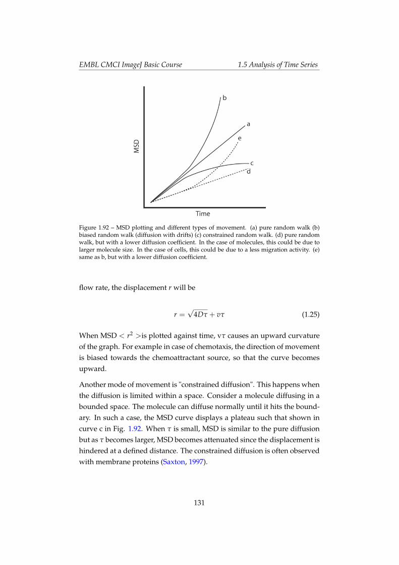
EMBL CMCI ImageJ Basic Course 1.5 Analysis of Time Series
Figure 1.92 – MSD plotting and different types of movement. (a) pure random walk (b)biased random walk (diffusion with drifts) (c) constrained random walk. (d) pure randomwalk, but with a lower diffusion coefficient. In the case of molecules, this could be due tolarger molecule size. In the case of cells, this could be due to a less migration activity. (e)same as b, but with a lower diffusion coefficient.
flow rate, the displacement r will be
r =√
4Dτ + vτ (1.25)
When MSD < r2 >is plotted against time, vτ causes an upward curvatureof the graph. For example in case of chemotaxis, the direction of movementis biased towards the chemoattractant source, so that the curve becomesupward.
Another mode of movement is "constrained diffusion". This happens whenthe diffusion is limited within a space. Consider a molecule diffusing in abounded space. The molecule can diffuse normally until it hits the bound-ary. In such a case, the MSD curve displays a plateau such that shown incurve c in Fig. 1.92. When τ is small, MSD is similar to the pure diffusionbut as τ becomes larger, MSD becomes attenuated since the displacement ishindered at a defined distance. The constrained diffusion is often observedwith membrane proteins (Saxton, 1997).
131

EMBL CMCI ImageJ Basic Course 1.5 Analysis of Time Series
1.5.9 ASSIGNMENTS
Assignments 1-5-5-2:
Open tubulin dynamics image stack kin_tubulin.stk and do manual track-ing like you did in the exercise 1.5.6. Track six points and plot the tracks ina same graph. Is there anything you can say about their dynamics?Images: courtesy of Puck Ohi.
132
References
C. M. Anderson, G. N. Georgiou, I. E. Morrison, G. V. Stevenson,and R. J. Cherry. Tracking of cell surface receptors by fluores-cence digital imaging microscopy using a charge-coupled devicecamera. low-density lipoprotein and influenza virus receptor mo-bility at 4 degrees c. J Cell Sci, 101 ( Pt 2):415–25, Feb 1992. URLhttp://www.ncbi.nlm.nih.gov/entrez/query.fcgi?cmd=
Retrieve&db=PubMed&dopt=Citation&list_uids=1629253.92332618 0021-9533 Journal Article.
H Berg. Random Walk in Biology. Princeton University Press, Princeton,1993.
S. Bolte and F. P. Cordelières. A guided tour into subcellular colocaliza-tion analysis in light microscopy. J Microsc, 224(Pt 3):213–232, Dec 2006.doi: 10.1111/j.1365-2818.2006.01706.x. URL http://dx.doi.org/10.
1111/j.1365-2818.2006.01706.x.
A. E. Carlsson, A. D. Shah, D. Elking, T. S. Karpova, and J. A. Cooper.Quantitative analysis of actin patch movement in yeast. Biophys J, 82(5):2333–43, May 2002. URL http://www.ncbi.nlm.nih.gov/entrez/query.fcgi?cmd=Retrieve&db=PubMed&dopt=Citation&list_
uids=11964224. 21961476 0006-3495 Journal Article.
M. K. Cheezum, W. F. Walker, and W. H. Guilford. Quan-titative comparison of algorithms for tracking single fluo-rescent particles. Biophys J, 81(4):2378–88, Oct 2001. URLhttp://www.ncbi.nlm.nih.gov/entrez/query.fcgi?cmd=
Retrieve&db=PubMed&dopt=Citation&list_uids=11566807.21450444 0006-3495 Journal Article.
EMBL CMCI ImageJ Basic Course REFERENCES
DW Cromey. Digital imaging: Ethics., 2007. URL http://swehsc.
pharmacy.arizona.edu/exppath/.
D. Dormann, T. Libotte, C. J. Weijer, and T. Bretschneider. Simultaneousquantification of cell motility and protein-membrane-association usingactive contours. Cell Motil Cytoskeleton, 52(4):221–30, Aug 2002. URLhttp://www.ncbi.nlm.nih.gov/entrez/query.fcgi?cmd=
Retrieve&db=PubMed&dopt=Citation&list_uids=12112136.22105498 0886-1544 Journal Article.
H. Geerts, M. De Brabander, R. Nuydens, S. Geuens, M. Moeremans,J. De Mey, and P. Hollenbeck. Nanovid tracking: a new automaticmethod for the study of mobility in living cells based on colloidal goldand video microscopy. Biophys J, 52(5):775–782, Nov 1987. doi: 10.1016/S0006-3495(87)83271-X. URL http://dx.doi.org/10.1016/
S0006-3495(87)83271-X.
J. Gelles, B. J. Schnapp, and M. P. Sheetz. Tracking kinesin-driven move-ments with nanometre-scale precision. Nature, 331(6155):450–3, Feb4 1988. URL http://www.ncbi.nlm.nih.gov/entrez/query.
fcgi?cmd=Retrieve&db=PubMed&dopt=Citation&list_uids=
3123999. 88122616 0028-0836 Journal Article.
R. N. Ghosh and W. W. Webb. Automated detection and trackingof individual and clustered cell surface low density lipoproteinreceptor molecules. Biophys J, 66(5):1301–18, May 1994. URLhttp://www.ncbi.nlm.nih.gov/entrez/query.fcgi?cmd=
Retrieve&db=PubMed&dopt=Citation&list_uids=8061186.94339330 0006-3495 Journal Article.
K. Hirschberg, C. M. Miller, J. Ellenberg, J. F. Presley, E. D. Siggia, R. D.Phair, and J. Lippincott-Schwartz. Kinetic analysis of secretory proteintraffic and characterization of golgi to plasma membrane transport in-termediates in living cells. J Cell Biol, 143(6):1485–503, Dec 14 1998. URLhttp://www.ncbi.nlm.nih.gov/entrez/query.fcgi?cmd=
Retrieve&db=PubMed&dopt=Citation&list_uids=9852146.99069477 0021-9525 Journal Article.
134
EMBL CMCI ImageJ Basic Course REFERENCES
A. Kusumi, Y. Sako, and M. Yamamoto. Confined lateral diffu-sion of membrane receptors as studied by single particle tracking(nanovid microscopy). effects of calcium-induced differentiation incultured epithelial cells. Biophys J, 65(5):2021–40, Nov 1993. URLhttp://www.ncbi.nlm.nih.gov/entrez/query.fcgi?cmd=
Retrieve&db=PubMed&dopt=Citation&list_uids=8298032.94128889 0006-3495 Journal Article.
D. S. Martin, M. B. Forstner, and J. A. Kas. Apparent subdiffusion inherentto single particle tracking. Biophys J, 83(4):2109–17, Oct 2002. URLhttp://www.ncbi.nlm.nih.gov/entrez/query.fcgi?cmd=
Retrieve&db=PubMed&dopt=Citation&list_uids=12324428.22235482 0006-3495 Journal Article.
K. Miura. Tracking movement in cell biology. In J. Rietdorf, editor, Advancesin Biochemical Engineering/Biotechnology, volume 95, page 267. SpringerVerlag, Heidelberg, 2005.
Kota Miura and Jens Rietdorf. Cell Imaging, chapter 3. Image quantificationand analysis, pages 49–72. Scion Publishing Ltd., 2006.
K. Murase, T. Fujiwara, Y. Umemura, K. Suzuki, R. Iino, H. Yamashita,M. Saito, H. Murakoshi, K. Ritchie, and A. Kusumi. Ultrafine mem-brane compartments for molecular diffusion as revealed by singlemolecule techniques. Biophys J, 86(6):4075–93, Jun 2004. URLhttp://www.ncbi.nlm.nih.gov/entrez/query.fcgi?cmd=
Retrieve&db=PubMed&dopt=Citation&list_uids=15189902.0006-3495 Journal Article.
R. J. Ober, S. Ram, and E. S. Ward. Localization accuracy in single-molecule microscopy. Biophys J, 86(2):1185–200, Feb 2004. URLhttp://www.ncbi.nlm.nih.gov/entrez/query.fcgi?cmd=
Retrieve&db=PubMed&dopt=Citation&list_uids=14747353.0006-3495 Evaluation Studies Journal Article.
J B Pawley. Handbook of biological confocal microscopy, volume 13 of Languageof science. Springer, 2006. ISBN 9780387259215. doi: 10.1117/1.600871.URL http://link.aip.org/link/?JBOPFO/13/029902/1.
135
EMBL CMCI ImageJ Basic Course REFERENCES
H. Qian, M. P. Sheetz, and E. L. Elson. Single particle tracking. analysis ofdiffusion and flow in two-dimensional systems. Biophys J, 60(4):910–21,Oct 1991. URL http://www.ncbi.nlm.nih.gov/entrez/query.
fcgi?cmd=Retrieve&db=PubMed&dopt=Citation&list_uids=
1742458. 92075891 0006-3495 Journal Article.
K. Ritchie and A. Kusumi. Single-particle tracking image microscopy. Meth-ods Enzymol, 360:618–34, 2003. URL http://www.ncbi.nlm.nih.
gov/entrez/query.fcgi?cmd=Retrieve&db=PubMed&dopt=
Citation&list_uids=12622171. 22509097 0076-6879 JournalArticle.
M. Rossner and K. M. Yamada. What’s in a picture? the temptationof image manipulation. J Cell Biol, 166(1):11–5, Jul 5 2004. URLhttp://www.ncbi.nlm.nih.gov/entrez/query.fcgi?cmd=
Retrieve&db=PubMed&dopt=Citation&list_uids=15240566.0021-9525 (Print) News.
M. J. Saxton. Single-particle tracking: the distribution of dif-fusion coefficients. Biophys J, 72(4):1744–53, Apr 1997. URLhttp://www.ncbi.nlm.nih.gov/entrez/query.fcgi?cmd=
Retrieve&db=PubMed&dopt=Citation&list_uids=9083678.97237200 0006-3495 Journal Article.
M. J. Saxton and K. Jacobson. Single-particle tracking: applications to mem-brane dynamics. Annu Rev Biophys Biomol Struct, 26:373–99, 1997. URLhttp://www.ncbi.nlm.nih.gov/entrez/query.fcgi?cmd=
Retrieve&db=PubMed&dopt=Citation&list_uids=9241424.97385410 1056-8700 Journal Article Review Review, Tutorial.
I. F. Sbalzarini and P. Koumoutsakos. Feature point tracking and trajectoryanalysis for video imaging in cell biology. J Struct Biol, 151(2):182–195,Aug 2005. doi: 10.1016/j.jsb.2005.06.002. URL http://dx.doi.org/
10.1016/j.jsb.2005.06.002.
B. J. Schnapp, J. Gelles, and M. P. Sheetz. Nanometer-scale measurementsusing video light microscopy. Cell Motil Cytoskeleton, 10(1-2):47–53,1988. URL http://www.ncbi.nlm.nih.gov/entrez/query.
136
EMBL CMCI ImageJ Basic Course REFERENCES
fcgi?cmd=Retrieve&db=PubMed&dopt=Citation&list_uids=
3141071. 89028766 0886-1544 Journal Article.
G. J. Schütz, H. Schindler, and T. Schmidt. Single-molecule microscopy onmodel membranes reveals anomalous diffusion. Biophys J, 73(2):1073–80,Aug 1997. URL http://www.ncbi.nlm.nih.gov/entrez/query.
fcgi?cmd=Retrieve&db=PubMed&dopt=Citation&list_uids=
9251823. 97395719 0006-3495 Journal Article.
Michael Schwarzfischer, Carsten Marr, Jan Krumsiek, and PS Hoppe.Efficient fluorescence image normalization for time lapse movies.In Microscopic Image Analysis with Applications in Biology, Heidel-berg, Germany, September 2, 2011, number x, pages 3–7, 2011. URLhttp://www.helmholtz-muenchen.de/fileadmin/CMB/PDF/
jkrumsiek/Schwarzfischer2011_imageprocessing.pdf.
M. P. Sheetz, S. Turney, H. Qian, and E. L. Elson. Nanometre-levelanalysis demonstrates that lipid flow does not drive membrane gly-coprotein movements. Nature, 340(6231):284–8, Jul 27 1989. URLhttp://www.ncbi.nlm.nih.gov/entrez/query.fcgi?cmd=
Retrieve&db=PubMed&dopt=Citation&list_uids=2747796.89314153 0028-0836 Journal Article.
J. Suh, M. Dawson, and J. Hanes. Real-time multiple-particle tracking:applications to drug and gene delivery. Adv Drug Deliv Rev, 57(1):63–78,Jan 2 2005. URL http://www.ncbi.nlm.nih.gov/entrez/query.
fcgi?cmd=Retrieve&db=PubMed&dopt=Citation&list_uids=
15518921. 0169-409x Journal Article Review.
C. Tardin, L. Cognet, C. Bats, B. Lounis, and D. Choquet. Di-rect imaging of lateral movements of ampa receptors in-side synapses. Embo J, 22(18):4656–65, Sep 15 2003. URLhttp://www.ncbi.nlm.nih.gov/entrez/query.fcgi?cmd=
Retrieve&db=PubMed&dopt=Citation&list_uids=12970178.22850113 0261-4189 Journal Article.
R. E. Thompson, D. R. Larson, and W. W. Webb. Precise nanometer localiza-tion analysis for individual fluorescent probes. Biophys J, 82(5):2775–83,May 2002. URL http://www.ncbi.nlm.nih.gov/entrez/query.
137
EMBL CMCI ImageJ Basic Course REFERENCES
fcgi?cmd=Retrieve&db=PubMed&dopt=Citation&list_uids=
11964263. 21961515 0006-3495 Journal Article.
W Wallace, L H Schaefer, and J R Swedlow. A workingperson’s guide to de-convolution in light microscopy. BioTechniques, 31(5):1076–8, 1080, 1082passim, November 2001. ISSN 0736-6205. URL http://www.ncbi.
nlm.nih.gov/pubmed/11730015.
Thomas Walter, David W Shattuck, Richard Baldock, Mark E Bastin,Anne E Carpenter, Suzanne Duce, Jan Ellenberg, Adam Fraser, NicholasHamilton, Steve Pieper, Mark A Ragan, Jurgen E Schneider, PavelTomancak, and Jean-Karim Hériché. Visualization of image data fromcells to organisms. Nat Methods, 7(3 Suppl):S26–S41, Mar 2010. doi:10.1038/nmeth.1431. URL http://dx.doi.org/10.1038/nmeth.
1431.
Jennifer C Waters. Accuracy and precision in quantitative fluorescencemicroscopy. J Cell Biol, 185(7):1135–1148, Jun 2009. doi: 10.1083/jcb.200903097. URL http://dx.doi.org/10.1083/jcb.200903097.
C. M. Witt, S. Raychaudhuri, B. Schaefer, A. K. Chakraborty, andE. A. Robey. Directed migration of positively selected thymo-cytes visualized in real time. PLoS Biol, 3(6):e160, Jun 2005. URLhttp://www.ncbi.nlm.nih.gov/entrez/query.fcgi?cmd=
Retrieve&db=PubMed&dopt=Citation&list_uids=15869324.1545-7885 Journal Article.
138

EMBL CMCI ImageJ Basic Course 1.6 Appendices
1.6 Appendices
1.6.1 App.1 Header Structure and Image Files
For TIFF format, detailed description could be found at:http://www.digitalpreservation.gov/formats//content/tiff_
tags.shtml
139

EMBL CMCI ImageJ Basic Course 1.6 Appendices
1.6.2 App.1.5 Installing Plug-In
ImageJ
To install Plug-In, download the Plug-In file (*.class or *.jar) and put the filein the "plugin" folder within ImageJ folder. ImageJ must be restarted to seethe plugin in the menu. By default, Plug-in appears under [Plugins]. Ifyou want to change the location of the plugin in the menu, one can changethe place by using [Plugins > Utilities > Control Panel].
If you have too many Plugins, there will be significant probability of socalled "Class conflicts". Classes are the modules in ImageJ and Plugins.If there are two identical classes in ImageJ, then these classes causes theconflict in the process. To avoid this, one could have multiple ImageJ andinstall Plugin in each of them for different purposes, that there will be noPlugin overloads.
Fiji
Select [Plugins > Install Plugins...] then choose the plugin file (.jaror .class file).
140

EMBL CMCI ImageJ Basic Course 1.6 Appendices
1.6.3 App.1.75 List of accompanying PDF
• ImageJ_Manual.pdf
ImageJ Manual written by Tony Collins@Cell Imaging Core facil-ity, Toronto Western Research Intsitute
• rossner_yamada.pdf
JCB paper about manipulation of image data.
• Time Series_Analyzer.pdf
Manual for the Time Series Analyzer PlugIn
• Manual Tracking plugin.pdf
Manual Tracker PlugIn manual
141

EMBL CMCI ImageJ Basic Course 1.6 Appendices
1.6.4 App.2 Measurement Options
Copied fromhttp://rsb.info.nih.gov/ij/docs/guide/userguide-27.html#
toc-Subsection-27.7
AreaArea of selection in square pixels or in calibrated square units (e.g., mm2,µm2, etc.) if Analyze . Set Scale. . . was used to spatially calibrate the image.
Mean Gray ValueAverage gray value within the selection. This is the sum of the gray valuesof all the pixels in the selection divided by the number of pixels. Reportedin calibrated units (e.g., optical density) if Analyze . Calibrate. . . was usedto calibrate the image. For RGB images, the mean is calculated by convert-ing each pixel to grayscale using the formulagray = (red + green + blue)/3orgray = 0.299red + 0.587green + 0.114blueif Weighted RGB Conversions is checked in Edit . Options . Conversions. . .
Standard DeviationStandard deviation of the gray values used to generate the mean gray value.Uses the Results table heading StdDev.
Modal Gray ValueMost frequently occurring gray value within the selection. Corresponds tothe highest peak in the histogram. Uses the heading Mode.
Min & Max Gray LevelMinimum and maximum gray values within the selection.
CentroidThe center point of the selection. This is the average of the x and y co-ordinates of all of the pixels in the image or selection. Uses the X and Yheadings.
Center of MassThis is the brightness-weighted average of the x and y coordinates all pix-els in the image or selection. Uses the XM and YM headings. These coordi-
142

EMBL CMCI ImageJ Basic Course 1.6 Appendices
nates are the first order spatial moments.
PerimeterThe length of the outside boundary of the selection. Uses the headingPerim.. With IJ1.44f and later, the perimeter of a composite selection iscalculated by decomposing it into individual selections. Note that the com-posite perimeter and the sum of the individual perimeters may be differentdue to use of different calculation methods.
Bounding RectangleThe smallest rectangle enclosing the selection. Uses the headings BX, BY,Width and Height, where BX and BY are the coordinates of the upper leftcorner of the rectangle.
Fit EllipseFits an ellipse to the selection. Uses the headings Major, Minor and Angle.Major and Minor are the primary and secondary axis of the best fitting el-lipse. Angle is the angle between the primary axis and a line parallel tothe X-axis of the image. The coordinates of the center of the ellipse are dis-played as X and Y if Centroid is checked. Note that ImageJ cannot calculatethe major and minor axis lengths if Pixel Aspect Ratio in the Analyze . SetScale. . . dialog is not 1.0. There are several ways to view the fitted ellipse:
1. The Edit . Selection . Fit Ellipse command replaces an area selectionwith the best fit ellipse.
2. The DrawEllipse macro draws (destructively) the best fit ellipse andthe major and minor axis.
3. Select Ellipses from the Show: drop-down menu in the particle ana-lyzer (Analyze . Analyze Particles. . . ) and it will draw the ellipse foreach particle in a separate window.
Shape DescriptorsCalculates and displays the following shape descriptors:
• Circularity4π Area
Perimeter2 with a value of 1.0 indicating a perfect circle. As the valueapproaches 0.0, it indicates an increasingly elongated shape. Valuesmay not be valid for very small particles. Uses the heading Circ.
143
EMBL CMCI ImageJ Basic Course 1.6 Appendices
• Aspect RatioThe aspect ratio of the particle"s fitted ellipse, i.e., [Major Axis]
[Minor Axis] . If FitEllipse is selected the Major and Minor axis are displayed. Uses theheading AR.
• Roundness4 [Area]
π[Major axis]2 or the inverse of Aspect Ratio. Uses the heading Round.
• Solidity[Area]
[Convex area] ; Note that the Edit. Selection . Convex Hull commandmakes an area selection convex.
Feret’s DiameterThe longest distance between any two points along the selection bound-ary, also known as maximum caliper. Uses the heading Feret. The angle(0− 180 degrees) of the Feret’s diameter is displayed as FeretAngle, as wellas the minimum caliper diameter (MinFeret). The length of the object"sprojection in the X (FeretX) and Y (FeretY) direction is also displayed.
Integrated DensityThe sum of the values of the pixels in the image or selection. This is equiv-alent to the product of Area and Mean Gray Value. With IJ1.44c and later,Raw integrated density (sum of pixel values) is displayed under the head-ing RawIntDen when Integrated density is enabled. The Dot Blot Analysistutorial demonstrates how to use this option to analyze a dot blot assay.
MedianThe median value of the pixels in the image or selection.
SkewnessThe third order moment about the mean. The documentation for the Mo-ment Calculator plugin explains how to interpret spatial moments. Usesthe heading Skew.
KurtosisThe fourth order moment about the mean. Uses the heading Kurt.
Area FractionFor thresholded images is the percentage of pixels in the image or selectionthat have been highlighted in red using Image . Adjust . Threshold. . . [T].
144
EMBL CMCI ImageJ Basic Course 1.6 Appendices
For non-thresholded images is the percentage of non-zero pixels. Uses theheading %Area.
Stack PositionThe position (slice, channel and frame) in the stack or hyperstack of theselection. Uses the headings Slice, Ch and Frame.
n.b.: For line selections the heading Length is created. For straight lineselections, Angle is recorded even if Fit Ellipse is unchecked. Also, note thatmeasurements that do not apply to certain selection types may be listed asNaN, In f inity or −In f inity.
The second part of the dialog controls measurement settings:
Limit to ThresholdIf checked, only thresholded pixels are included in measurement calcula-tions. Use Image . Adjust . Threshold. . . [T] to set the threshold limits. Thissetting affects only thresholded images (see Settings and Preferences).
Display LabelIf checked, the image name and slice number (for stacks) are recorded inthe first column of the results table, e.g., mri-stack.tif:9. For renamed se-lections (Edit . Selection . Properties. . . [y]) or selections measured via ROIManager"s measure command (see ROI Manager. . . ), the selection label isappended, e.g., blobs.gif:0339-0163 or blobs.gif:mySelection.
Invert Y CoordinatesIf checked, the XY origin is assumed to be the lower left corner of the imagewindow instead of the upper left corner (see also Image . Properties. . . [P]).
Scientific NotationIf checked, measurements are displayed in scientific notation, e.g., 1.48E2.
Redirect ToThe image selected from this pop-up menu will be used as the target forstatistical calculations done by Analyze . Measure. . . [m] and Analyze .
Analyze Particles. . . commands. This feature allows you to outline a struc-ture on one image and measure the intensity of the corresponding regionin another image.
Decimal Places
145

EMBL CMCI ImageJ Basic Course 1.6 Appendices
This is the number of digits to the right of the decimal point in real numbersdisplayed in the Results table and in Histogram windows.
146

EMBL CMCI ImageJ Basic Course 1.6 Appendices
1.6.5 App.3 Edge Detection Principle
Quote from MBL manual:
One way to find boundaries of objects is to detect discontinu-ities in intensity values at the edge of a region. These disconti-nuities can be found by calculating the first and/or second or-der derivatives of an image. The first derivative of choice inimage processing is the gradient, defined as the vector:
grad f = [GxGy]
where Gx = d f /dx and Gy = d f /dy are the partial derivativesin the horizontal and vertical directions of the image. The mag-nitude of this vector is
|grad f | = (G2x + G2
y)1/2
The gradient vector points in the direction of steepest ascent.The angle of steepest ascent is given by:
a(x, y) = tan−1(Gx/Gy)
We can estimate the derivatives Gx and Gy digitally by linearlyfiltering the image with the following 3 by 3 kernels:
147

EMBL CMCI ImageJ Basic Course 1.6 Appendices
The Prewitt and Sobel operators are among the most used inpractice for computing digital gradients. The Prewitt masks aresimpler to implement than the Sobel masks, but the latter haveslightly superior noise-suppression characteristics.
148

EMBL CMCI ImageJ Basic Course 1.6 Appendices
1.6.6 App.4 Particle Tracker manual
Tutorial from : http://weeman.inf.ethz.ch/particletracker/tutorial.html
PDF inserted from next page.
149
ParticleTracker - Tutorial The ParticleTracker is an ImageJ Plugin for multiple particle detection and tracking from digital videos
Sample Data and Tutorial
This tutorial provides a basic introduction on how to select the right parameters for the algorithm of ParticleTracker and the right display and analysis options upon completion of it.
Written by Guy Levy at the Computational Biophysics Lab, ETH Zurich
To use this tutorial you should already be familiar with ImageJ and have the plugin installed. It is also recommended to read the user manual before starting. In this tutorial we will guide you through an example using movies sample data:
• TransportOfEndosomalVirus.zip - a real experimental movie (image sequence) from Suomalainen et al., J. Cell Biol. 144 (4): 657-672 Kindly provided by The Cell Biology group, Institute of Zoology, University of Zurich. Fast minus and plus end-directed transport of endosomal ts1 virus labeled with Texas red. Virus was added to TC7/MAP4/MTB-GFP cells and 72 TR-images were recorded with intervals of 1.5 s starting 20 min p.i.. The GFP signal is indicated at the beginning. Bar = 10 µm
• Artificial.zip - Artificial image sequence, will be used later in the tutorial for a specific example
• First Step - download sample movie and open it • Second Step - select particle detection parameters and preview • Third Step - viewing the results • Fourth Step - re linking the particles
First Step - download sample movie and open it
Download the TransportOfEndosomalVirus.zip file. Both the movies are actually sequence of separate image files (.tif) all in a zipped folder. After downloading the zip file, unzip it to your preferred folder and Start ImageJ. Load the image sequence by selecting the Import -> Image Sequence… from the File menu.
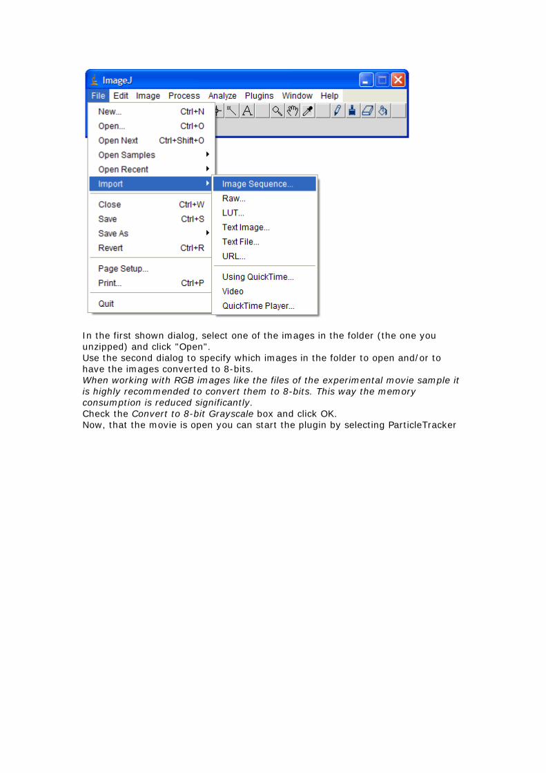
In the first shown dialog, select one of the images in the folder (the one you unzipped) and click "Open". Use the second dialog to specify which images in the folder to open and/or to have the images converted to 8-bits. When working with RGB images like the files of the experimental movie sample it is highly recommended to convert them to 8-bits. This way the memory consumption is reduced significantly. Check the Convert to 8-bit Grayscale box and click OK. Now, that the movie is open you can start the plugin by selecting ParticleTracker
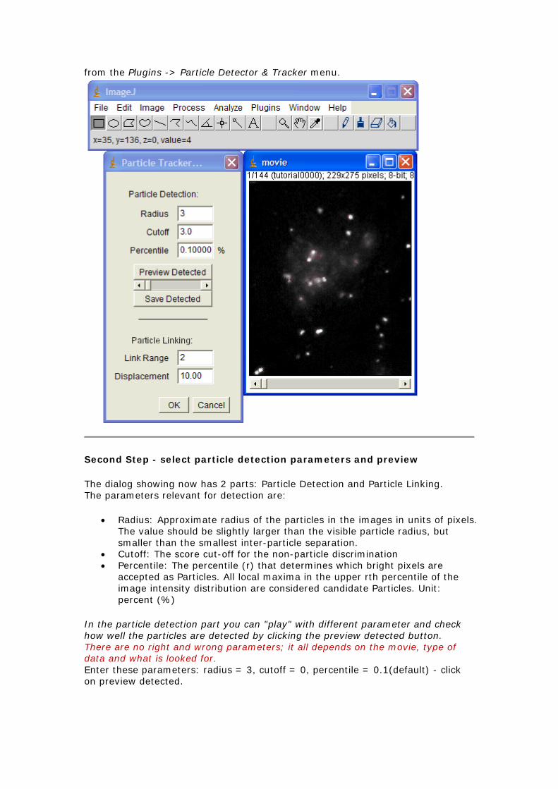
from the Plugins -> Particle Detector & Tracker menu.
Second Step - select particle detection parameters and preview
The dialog showing now has 2 parts: Particle Detection and Particle Linking. The parameters relevant for detection are:
• Radius: Approximate radius of the particles in the images in units of pixels. The value should be slightly larger than the visible particle radius, but smaller than the smallest inter-particle separation.
• Cutoff: The score cut-off for the non-particle discrimination • Percentile: The percentile (r) that determines which bright pixels are
accepted as Particles. All local maxima in the upper rth percentile of the image intensity distribution are considered candidate Particles. Unit: percent (%)
In the particle detection part you can "play" with different parameter and check how well the particles are detected by clicking the preview detected button. There are no right and wrong parameters; it all depends on the movie, type of data and what is looked for. Enter these parameters: radius = 3, cutoff = 0, percentile = 0.1(default) - click on preview detected.
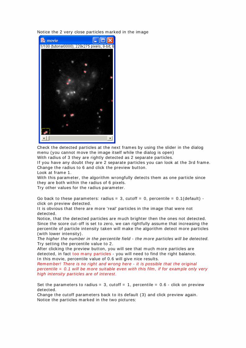
Notice the 2 very close particles marked in the image
Check the detected particles at the next frames by using the slider in the dialog menu (you cannot move the image itself while the dialog is open) With radius of 3 they are rightly detected as 2 separate particles. If you have any doubt they are 2 separate particles you can look at the 3rd frame. Change the radius to 6 and click the preview button. Look at frame 1. With this parameter, the algorithm wrongfully detects them as one particle since they are both within the radius of 6 pixels. Try other values for the radius parameter.
Go back to these parameters: radius = 3, cutoff = 0, percentile = 0.1(default) - click on preview detected. It is obvious that there are more 'real' particles in the image that were not detected. Notice, that the detected particles are much brighter then the ones not detected. Since the score cut-off is set to zero, we can rightfully assume that increasing the percentile of particle intensity taken will make the algorithm detect more particles (with lower intensity). The higher the number in the percentile field - the more particles will be detected. Try setting the percentile value to 2. After clicking the preview button, you will see that much more particles are detected, in fact too many particles - you will need to find the right balance. In this movie, percentile value of 0.6 will give nice results. Remember! There is no right and wrong here - it is possible that the original percentile = 0.1 will be more suitable even with this film, if for example only very high intensity particles are of interest.
Set the parameters to radius = 3, cutoff = 1, percentile = 0.6 - click on preview detected. Change the cutoff parameters back to its default (3) and click preview again. Notice the particles marked in the two pictures:
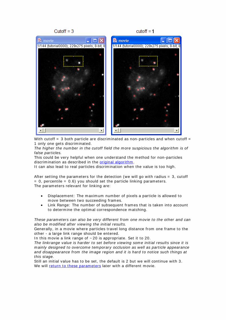
With cutoff = 3 both particle are discriminated as non-particles and when cutoff = 1 only one gets discriminated. The higher the number in the cutoff field the more suspicious the algorithm is of false particles. This could be very helpful when one understand the method for non-particles discrimination as described in the original algorithm. It can also lead to real particles discrimination when the value is too high.
After setting the parameters for the detection (we will go with radius = 3, cutoff = 0, percentile = 0.6) you should set the particle linking parameters. The parameters relevant for linking are:
• Displacement: The maximum number of pixels a particle is allowed to move between two succeeding frames.
• Link Range: The number of subsequent frames that is taken into account to determine the optimal correspondence matching.
These parameters can also be very different from one movie to the other and can also be modified after viewing the initial results. Generally, in a movie where particles travel long distance from one frame to the other - a large link range should be entered. In this movie a link range of ~20 is appropriate. Set it to 20. The linkrange value is harder to set before viewing some initial results since it is mainly designed to overcome temporary occlusion as well as particle appearance and disappearance from the image region and it is hard to notice such things at this stage. Still an initial value has to be set, the default is 2 but we will continue with 3. We will return to these parameters later with a different movie.

You can now go ahead with the linking by clicking OK. The progress of the algorithm will be displayed in the main ImageJ Status Bar.
Third Step - viewing the results
After completing the particle tracking, the result window will be displayed. Click the Visualize all Trajectories button to view all the found trajectories.
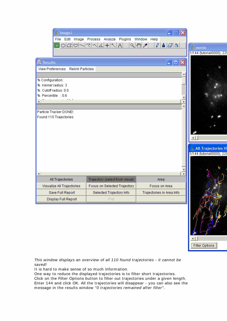
This window displays an overview of all 110 found trajectories - it cannot be saved! It is hard to make sense of so much information. One way to reduce the displayed trajectories is to filter short trajectories. Click on the Filter Options button to filter out trajectories under a given length. Enter 144 and click OK. All the trajectories will disappear - you can also see the message in the results window "0 trajectories remained after filter".
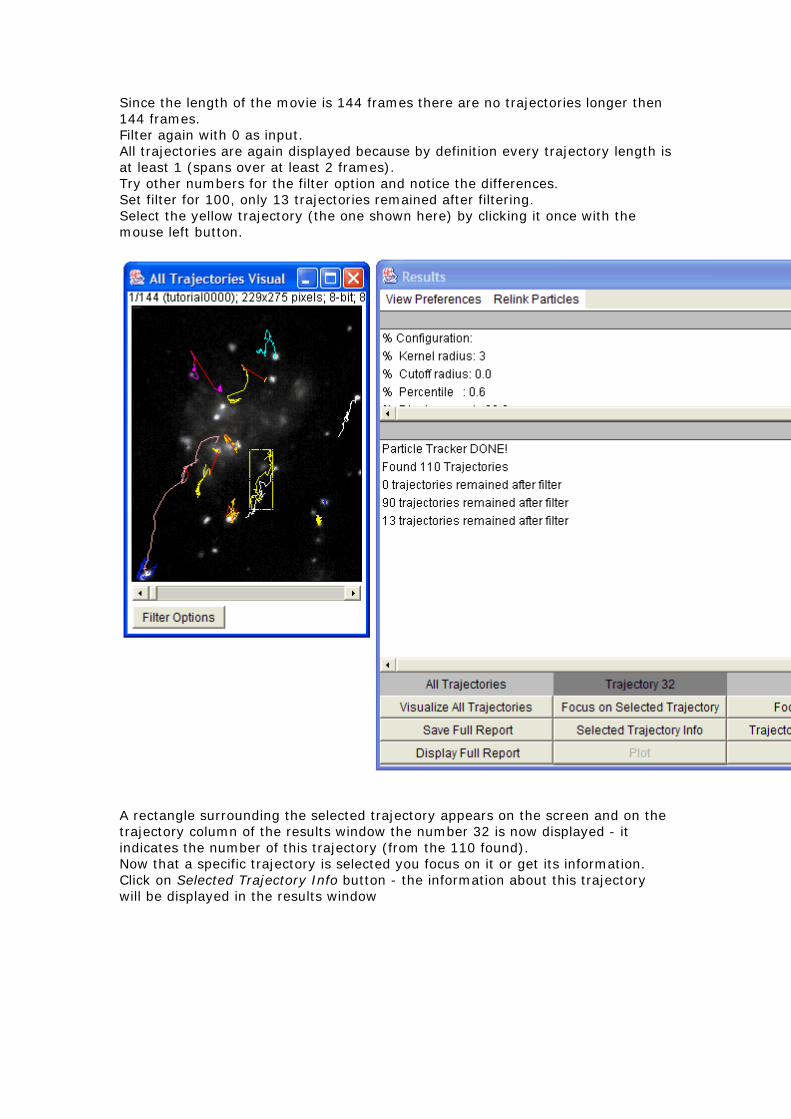
Since the length of the movie is 144 frames there are no trajectories longer then 144 frames. Filter again with 0 as input. All trajectories are again displayed because by definition every trajectory length is at least 1 (spans over at least 2 frames). Try other numbers for the filter option and notice the differences. Set filter for 100, only 13 trajectories remained after filtering. Select the yellow trajectory (the one shown here) by clicking it once with the mouse left button.
A rectangle surrounding the selected trajectory appears on the screen and on the trajectory column of the results window the number 32 is now displayed - it indicates the number of this trajectory (from the 110 found). Now that a specific trajectory is selected you focus on it or get its information. Click on Selected Trajectory Info button - the information about this trajectory will be displayed in the results window
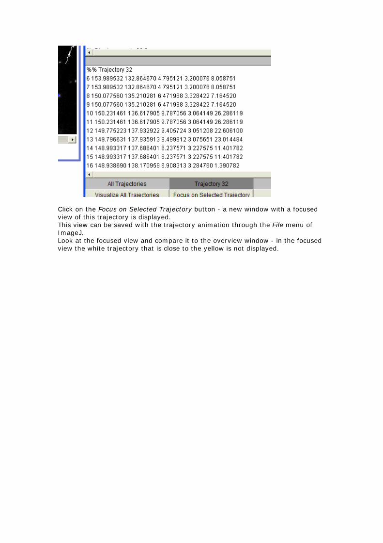
Click on the Focus on Selected Trajectory button - a new window with a focused view of this trajectory is displayed. This view can be saved with the trajectory animation through the File menu of ImageJ. Look at the focused view and compare it to the overview window - in the focused view the white trajectory that is close to the yellow is not displayed.
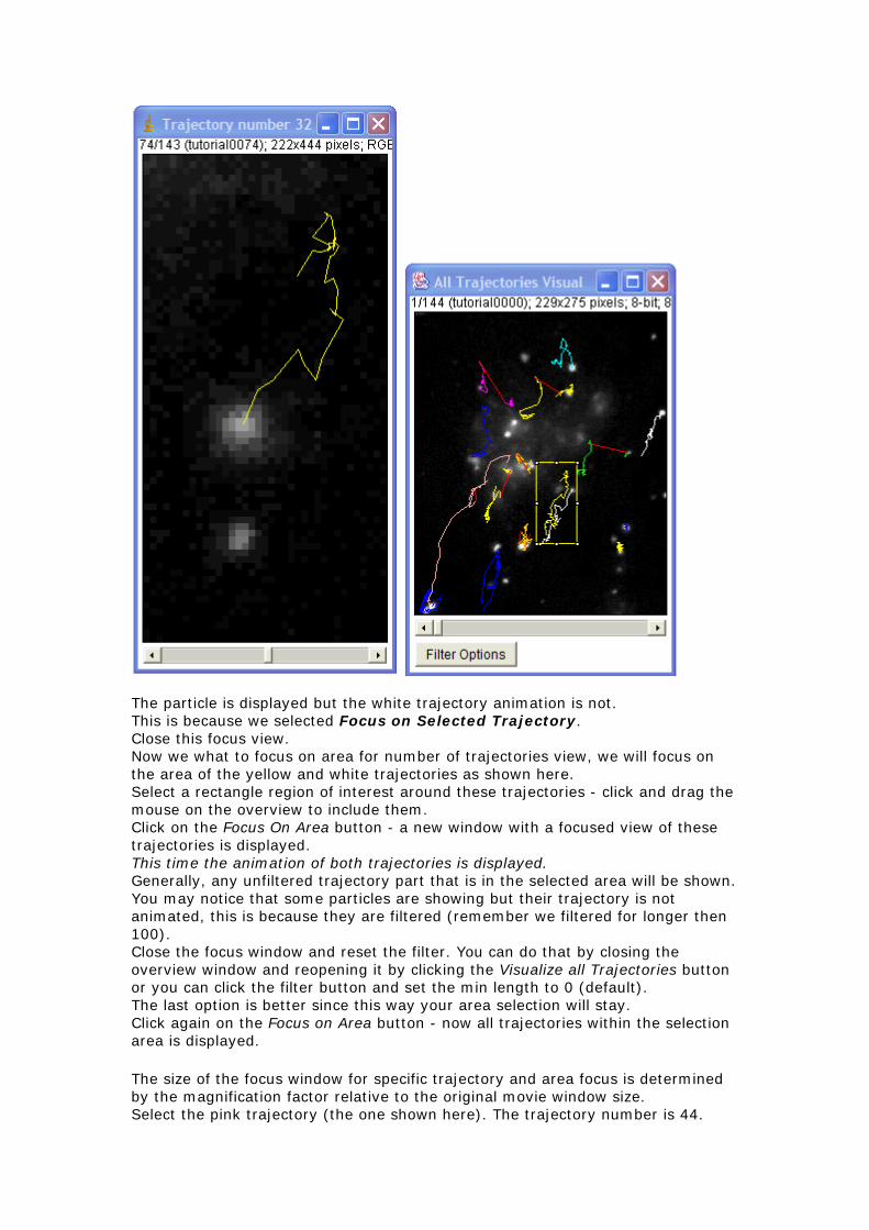
The particle is displayed but the white trajectory animation is not. This is because we selected Focus on Selected Trajectory. Close this focus view. Now we what to focus on area for number of trajectories view, we will focus on the area of the yellow and white trajectories as shown here. Select a rectangle region of interest around these trajectories - click and drag the mouse on the overview to include them. Click on the Focus On Area button - a new window with a focused view of these trajectories is displayed. This time the animation of both trajectories is displayed. Generally, any unfiltered trajectory part that is in the selected area will be shown. You may notice that some particles are showing but their trajectory is not animated, this is because they are filtered (remember we filtered for longer then 100). Close the focus window and reset the filter. You can do that by closing the overview window and reopening it by clicking the Visualize all Trajectories button or you can click the filter button and set the min length to 0 (default). The last option is better since this way your area selection will stay. Click again on the Focus on Area button - now all trajectories within the selection area is displayed.
The size of the focus window for specific trajectory and area focus is determined by the magnification factor relative to the original movie window size. Select the pink trajectory (the one shown here). The trajectory number is 44.
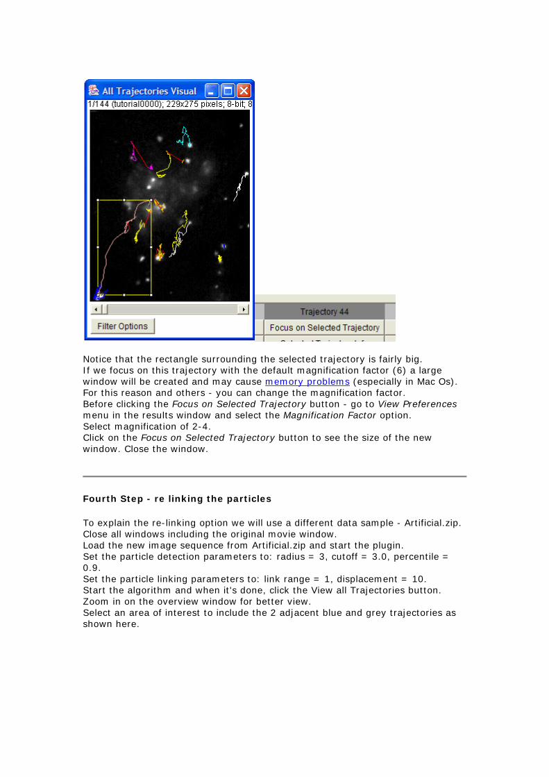
Notice that the rectangle surrounding the selected trajectory is fairly big. If we focus on this trajectory with the default magnification factor (6) a large window will be created and may cause memory problems (especially in Mac Os). For this reason and others - you can change the magnification factor. Before clicking the Focus on Selected Trajectory button - go to View Preferences menu in the results window and select the Magnification Factor option. Select magnification of 2-4. Click on the Focus on Selected Trajectory button to see the size of the new window. Close the window.
Fourth Step - re linking the particles
To explain the re-linking option we will use a different data sample - Artificial.zip. Close all windows including the original movie window. Load the new image sequence from Artificial.zip and start the plugin. Set the particle detection parameters to: radius = 3, cutoff = 3.0, percentile = 0.9. Set the particle linking parameters to: link range = 1, displacement = 10. Start the algorithm and when it's done, click the View all Trajectories button. Zoom in on the overview window for better view. Select an area of interest to include the 2 adjacent blue and grey trajectories as shown here.
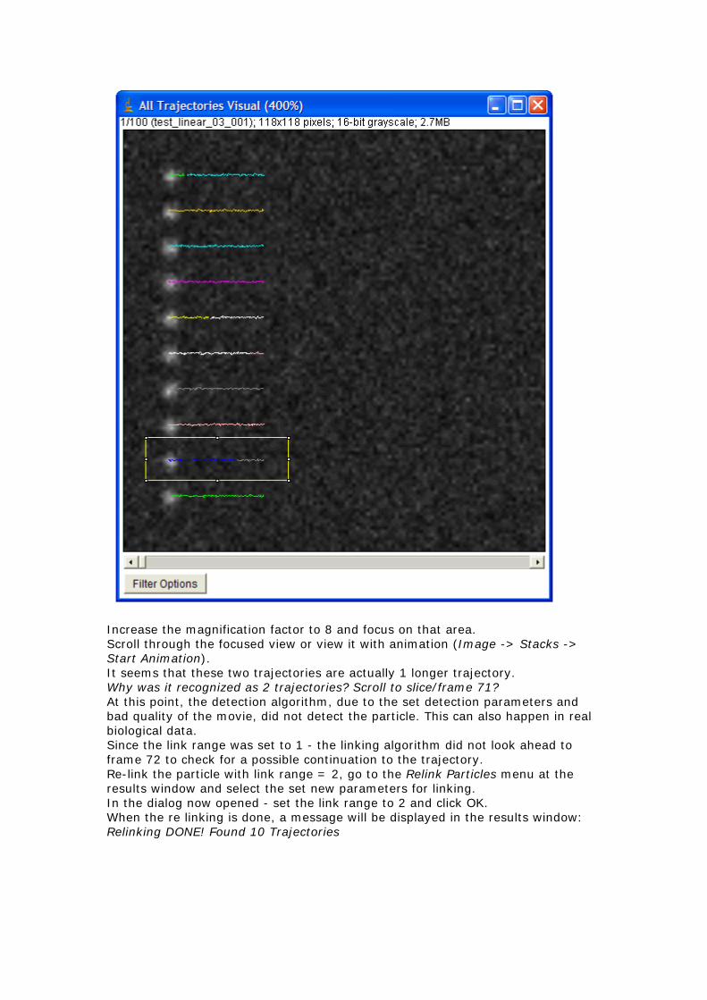
Increase the magnification factor to 8 and focus on that area. Scroll through the focused view or view it with animation (Image -> Stacks -> Start Animation). It seems that these two trajectories are actually 1 longer trajectory. Why was it recognized as 2 trajectories? Scroll to slice/frame 71? At this point, the detection algorithm, due to the set detection parameters and bad quality of the movie, did not detect the particle. This can also happen in real biological data. Since the link range was set to 1 - the linking algorithm did not look ahead to frame 72 to check for a possible continuation to the trajectory. Re-link the particle with link range = 2, go to the Relink Particles menu at the results window and select the set new parameters for linking. In the dialog now opened - set the link range to 2 and click OK. When the re linking is done, a message will be displayed in the results window: Relinking DONE! Found 10 Trajectories
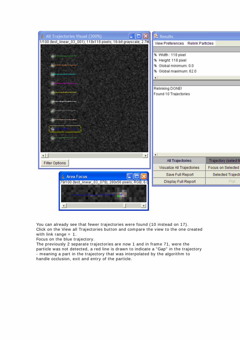
You can already see that fewer trajectories were found (10 instead on 17). Click on the View all Trajectories button and compare the view to the one created with link range = 1. Focus on the blue trajectory. The previously 2 separate trajectories are now 1 and in frame 71, were the particle was not detected, a red line is drawn to indicate a "Gap" in the trajectory - meaning a part in the trajectory that was interpolated by the algorithm to handle occlusion, exit and entry of the particle.
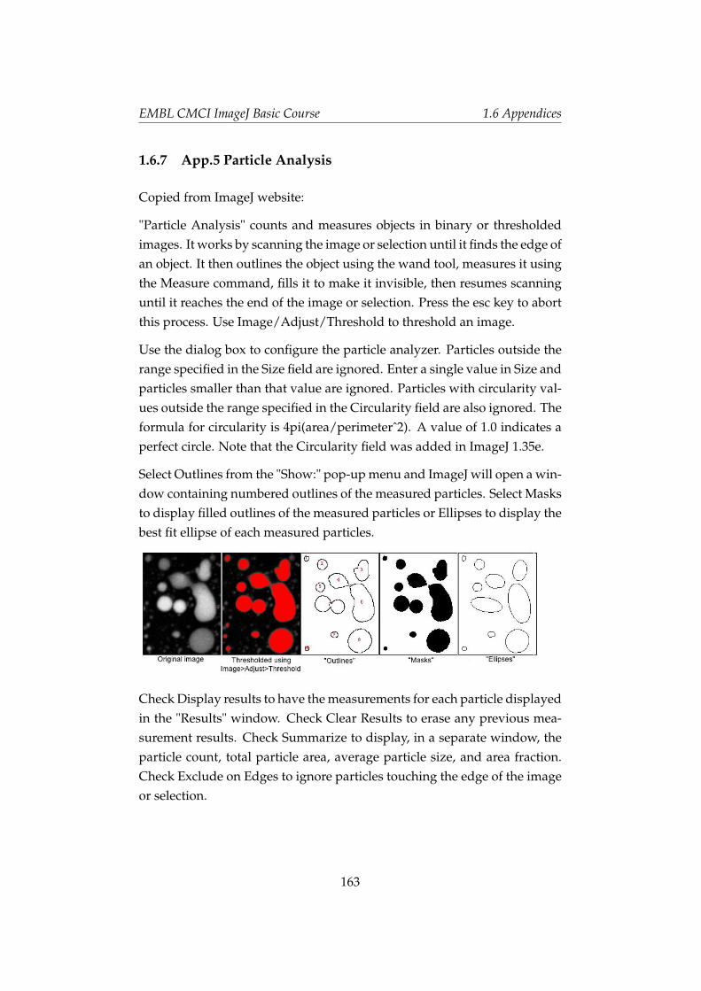
EMBL CMCI ImageJ Basic Course 1.6 Appendices
1.6.7 App.5 Particle Analysis
Copied from ImageJ website:
"Particle Analysis" counts and measures objects in binary or thresholdedimages. It works by scanning the image or selection until it finds the edge ofan object. It then outlines the object using the wand tool, measures it usingthe Measure command, fills it to make it invisible, then resumes scanninguntil it reaches the end of the image or selection. Press the esc key to abortthis process. Use Image/Adjust/Threshold to threshold an image.
Use the dialog box to configure the particle analyzer. Particles outside therange specified in the Size field are ignored. Enter a single value in Size andparticles smaller than that value are ignored. Particles with circularity val-ues outside the range specified in the Circularity field are also ignored. Theformula for circularity is 4pi(area/perimeterˆ2). A value of 1.0 indicates aperfect circle. Note that the Circularity field was added in ImageJ 1.35e.
Select Outlines from the "Show:" pop-up menu and ImageJ will open a win-dow containing numbered outlines of the measured particles. Select Masksto display filled outlines of the measured particles or Ellipses to display thebest fit ellipse of each measured particles.
Check Display results to have the measurements for each particle displayedin the "Results" window. Check Clear Results to erase any previous mea-surement results. Check Summarize to display, in a separate window, theparticle count, total particle area, average particle size, and area fraction.Check Exclude on Edges to ignore particles touching the edge of the imageor selection.
163
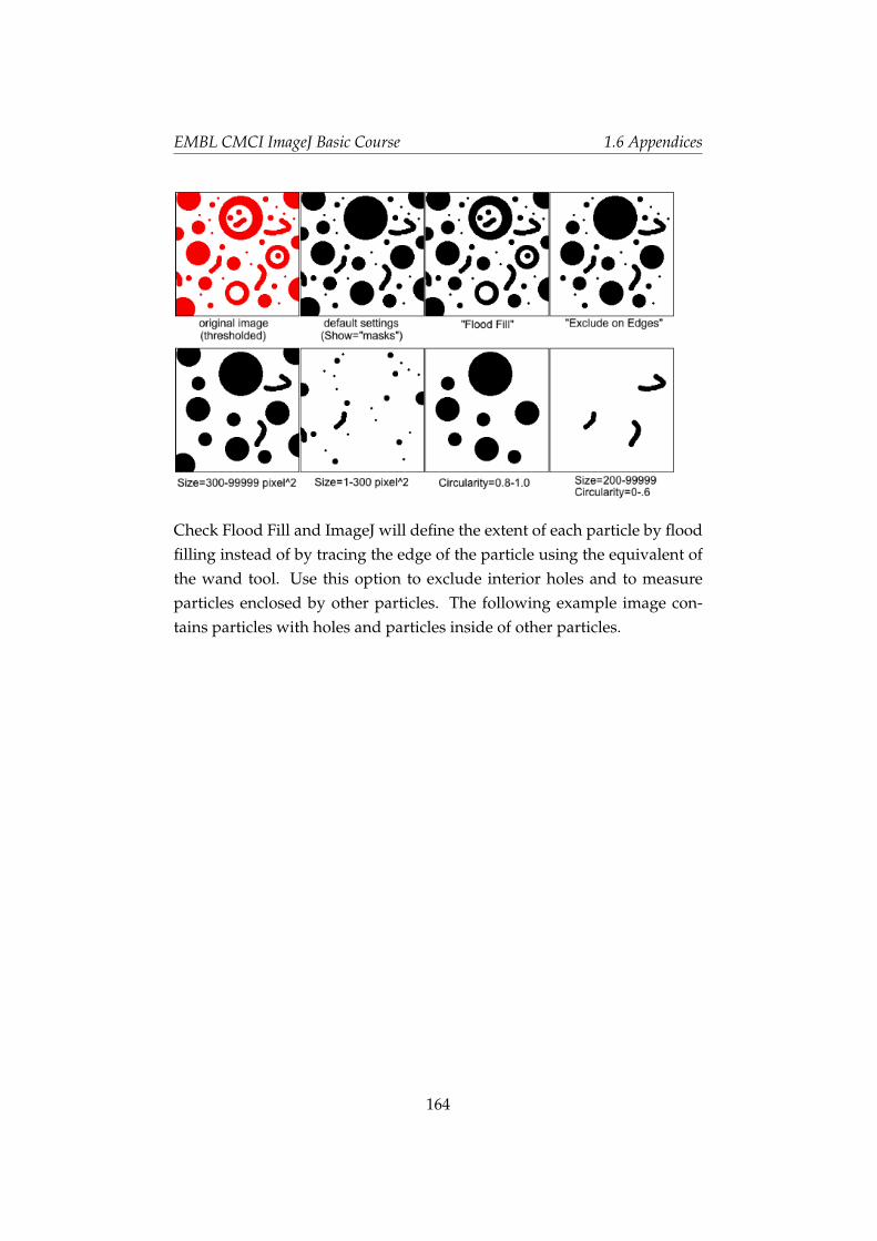
EMBL CMCI ImageJ Basic Course 1.6 Appendices
Check Flood Fill and ImageJ will define the extent of each particle by floodfilling instead of by tracing the edge of the particle using the equivalent ofthe wand tool. Use this option to exclude interior holes and to measureparticles enclosed by other particles. The following example image con-tains particles with holes and particles inside of other particles.
164
EMBL CMCI ImageJ Basic Course 1.6 Appendices
1.6.8 App.6 Image Processing and Analysis: software, scriptinglanguage
ImageJ is not only the tool for scientific image processing and analysis. Ilist some other software and tools used by EMBL researchers here and addsome description about each of them. For more details, please refer to anarticle by Walter et al. (2010).
MatLab (Mathworks), $
With Matlab, you could access images as numerical matrix to do process-ing and analysis of images. Programming is possible with Matlab scriptinglanguage. Scripts could be kept as files and execute them directly from theMatlab command line. These files are called "m-files". Many imaging re-lated tools are publicly available via Internet download. Scripts could beexported as execution files, and could be distributed without Matlab itself,as these stand-alone execution files only require freely available Matlab li-brary. A free alternative is Octave. I have never tried this yet, but thisfreeware is under extensive development and worth for some trial.
Imaris (Bitplane), $
Imaris is also a commercial software, especially powerful in interactive 3Dvisualization. 3D time course (sometimes called "4D") with multiple chan-nels (then this would be called 5D) could also be visualized and interac-tively adjusted with their appearance. Some analysis packages are option-ally available. I sometimes use optional package "Imaris Track" for track-ing spotty signals. Algorithm for linking particles is excellent (uses graph-theory based algorithm developed in Danuser lab). In EMBL, you couldtry using this software by so called "floating license", which enables you touse the software from any computer within EMBL domain. The number ofsimultaneous usage is limited to three (as of June 2010). Another modulethat gives additional power to Imaris is "Imaris XT", which enables access-ing Imaris objects from Matlab, Java or ImageJ. I have some example Javacodes, so if you are interested I could give you as an example. Imaris ispretty expensive, and apparent disadvantage.
Python, Free
165

EMBL CMCI ImageJ Basic Course 1.6 Appendices
Python is not a software package, but is a scripting language. There aremany other scripting languages like Ruby, but the merit of Python is thatthere are numerous libraries for image processing and analysis. In termsof scripting, accessibility is similar or more powerful than Matlab, since itsbridging capability to many computer languages such as C, C++ and Java.Considering that the trend of image processing and analysis is getting moreand more towards cross-language library usage, Python is a good choice tolearn for high-end processing and analysis.
Cell Profiler, Free
This free software is a bit less with available functions compared to Im-ageJ, but is easier and robust in constructing pipelines for image process-ing and analysis. One could interactively construct pipeline and do high-throughput processing and analysis for many data.
166
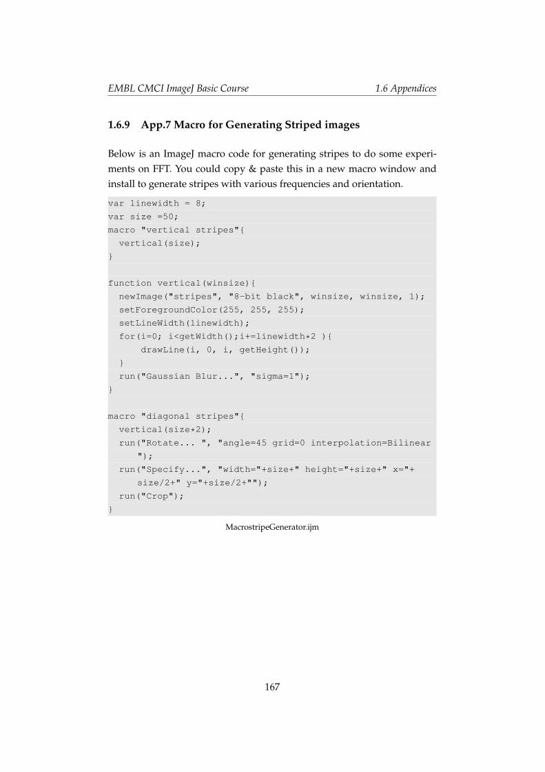
EMBL CMCI ImageJ Basic Course 1.6 Appendices
1.6.9 App.7 Macro for Generating Striped images
Below is an ImageJ macro code for generating stripes to do some experi-ments on FFT. You could copy & paste this in a new macro window andinstall to generate stripes with various frequencies and orientation.
var linewidth = 8;
var size =50;
macro "vertical stripes"
vertical(size);
function vertical(winsize)
newImage("stripes", "8-bit black", winsize, winsize, 1);
setForegroundColor(255, 255, 255);
setLineWidth(linewidth);
for(i=0; i<getWidth();i+=linewidth*2 )
drawLine(i, 0, i, getHeight());
run("Gaussian Blur...", "sigma=1");
macro "diagonal stripes"
vertical(size*2);
run("Rotate... ", "angle=45 grid=0 interpolation=Bilinear
");
run("Specify...", "width="+size+" height="+size+" x="+
size/2+" y="+size/2+"");
run("Crop");
MacrostripeGenerator.ijm
167

EMBL CMCI ImageJ Basic Course 1.6 Appendices
1.6.10 App.8 Deconvolution Exercise
Exercise starts from next page.
In this exercise, following plugins are used. If you do not have them inyour ImageJ or Fiji, download them and install. Deconvolution lab cannotbe installed by [Plugins > Install]. Unpack the downloaded zip folderand place all the contents under plugins directory.
1. PSFgenerator http://bigwww.epfl.ch/algorithms/psfgenerator/
2. DeconvolutionLab http://bigwww.epfl.ch/algorithms/deconvolution/
168

Excercises on deconvolution
Alessandra Griffa
September 1, 2010
Exercise 1: 3D widefield PSF
Start the PSFGenerator plugin in ImageJ. Generate a 3D PSF for a widefield microscope with
following parameters:
• ni =.1.518
• NA = 1.4
• W040 = 0
• λ =500nm
• amplitude = 255
• background = 0
• SNR= 100
• x0 = y0 = 32
• z0 = 64
• Δr = Δz = 50nm
• Nx = Ny = 64
• Nz =128
You can discard the image called PSF for deconvolution. Browse through the PSF using the
VolumeViewer, the 3D Viewer and the Orthogonal Views tools of ImageJ. (hint: change the
lookup table of the optic PSF into Fire to better appreciate its shape)
Change the numerical aperture (e.g. NA = 0.8) and/or the wavelength (e.g. λ = 400 or 600
nm). Generate the corresponding PSFs and describe the influence of these parameters.

Go back to the initial set of parameters. W040 controls the amount of spherical aberrations;
set its value to 500 nm. Describe the effect on the PSF. What are possible causes of spherical
aberrations?
Exercise 2: 2D inverse filtering
Load the images FluorescentCells.tif and PSFDefocus.tif. Launch the Deconvolution plugin.
2.1 Noise-free inverse filtering
We will first create an artificially blurred image using the defocusing blur kernel.
In the PSF section of the plugin, select the image PSFDefocus.tif. Make sure that Normalize
PSF is selected. In the Algorithm section, select Convolution. Make sure that Add noise is
deselected. Click the Run button. (note: to apply the plugin’s functionalities to a specific
image, you have to make sure that it was the last active image before clicking Run)
Try to deconvolve the widefield image you simulated using the inverse filtering method. In
the Algorithm section, select Direct inversion and click Run. Comment the result.
2.2 Noisy inverse and Wiener filtering
We will create now an artificially blurred and noisy image (more realistic simulation).
Go back to Convolution in the Algorithm section. Activate the Add noise checkbox. Play
around with both noise models at various noise levels (e.g. between 10, 30 and 60 dB), to get
a feeling for this functionality. What are the principal sources of Gaussian and Poisson noise
in microscopy images?

Choose the Gaussian model with a noise level such that you cannot visually distinguish the
image from the one obtained at point 2.1. Apply the inverse filtering to restore the image and
comment the results.
Try now the inverse filtering with regularization (Wiener filtering) on the noisy and blurred
image. Select Regularized Direct Inversion in the Algorithm section and run the
deconvolution with different values of the regularization parameter Lambda. How does the
regularization parameter influence the result?
Exercise 3: 2D iterative deconvolution
Choose the Poisson model with a noise level of 30 dB. Select the Richardson-Lucy
deconvolution algorithm, which is one of the simplest deconvolution algorithms for shot-
noise limited imaging. Try out the algorithm with different numbers of iterations (no more
than 100). What is the optimal number of iterations?
Suggestion: you can obtain a quantitative assessment of your prediction as follows (keep in
mind that this is a synthetic experiment!): under Log, choose Normal; under SER, choose
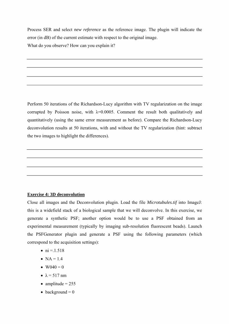
Process SER and select new reference as the reference image. The plugin will indicate the
error (in dB) of the current estimate with respect to the original image.
What do you observe? How can you explain it?
Perform 50 iterations of the Richardson-Lucy algorithm with TV regularization on the image
corrupted by Poisson noise, with λ=0.0005. Comment the result both qualitatively and
quantitatively (using the same error measurement as before). Compare the Richardson-Lucy
deconvolution results at 50 iterations, with and without the TV regularization (hint: subtract
the two images to highlight the differences).
Exercise 4: 3D deconvolution
Close all images and the Deconvolution plugin. Load the file Microtubules.tif into ImageJ:
this is a widefield stack of a biological sample that we will deconvolve. In this exercise, we
generate a synthetic PSF; another option would be to use a PSF obtained from an
experimental measurement (typically by imaging sub-resolution fluorescent beads). Launch
the PSFGenerator plugin and generate a PSF using the following parameters (which
correspond to the acquisition settings):
• ni =.1.518
• NA = 1.4
• W040 = 0
• λ = 517 nm
• amplitude = 255
• background = 0

• SNR= 100
• x0 = y0 = 144
• z0 = 192
• Δr = 89 nm
• Δz = 290 nm
• Nx = 288
• Ny = 384
• Nz = 32
•
Perform a visual verification of the Optic PSF stack; after that you can discard it.
Note that the voxel size of the acquired image is coherent with the resolution of an objective
with 1.4 NA, for the used wavelength.
Open the Deconvolution plugin. In the PSF section, select PSF for deconvolution. In the
Algorithm section, select the Richardson-Lucy algorithm with 20 iterations. Compute
maximum intensity projections of the original and deconvolved stacks. Compare them.
If there is some time left: try to perform a deconvolution with another algorithm (e.g. the
Tikhonov-Miller algorithm) and comment the results. You may want to activate Test the
algorithm on a small rectangular selection. You could also study the influence of using a PSF
with wrong parameters (for example, change the NA value or introduce spherical aberrations).


![Whole Genome Shatqun updates) C] EMBL (Cantiq release) C] EMBL (Coding Sequences) C] Genome Reviews C] EMBL ID/ Accession Mapping C] EMBL MGA Nucleotide sequence databases - subsections](https://img.pdfslide.us/doc/110x75/5ccc4c0c88c993de558c2477/whole-genome-shatqun-updates-c-embl-cantiq-release-c-embl-coding-sequences.jpg)