E

Va

b

a

ARR2AA

KPMIDT

1

esug&c(aiiattfwsusor

0h

Computers and Chemical Engineering 53 (2013) 35– 43

Contents lists available at SciVerse ScienceDirect

Computers and Chemical Engineering

jo u rn al hom epa ge : www.elsev ier .com/ locate /compchemeng

mbedding structural information in simulation-based optimization

idar Gunneruda,∗, Andrew Connb, Bjarne Fossa

Norwegian University of Science and Technology, NorwayIBM Thomas J. Watson Research Center, New York, USA

r t i c l e i n f o

rticle history:eceived 7 January 2012eceived in revised form7 November 2012ccepted 1 February 2013vailable online 27 February 2013

eywords:etroleum production optimization

a b s t r a c t

This paper proposes and explores an algorithm designed to find optimal settings for a process network.Emphasis is put on the system being divisible into components, as this underlying assumption motivatesthe algorithm in its entirety in that rather simple relations between the system components are modeledas explicit structural constraints, while the significantly more complex relations within each componentare approximated based on the underlying simulator data. Although the approach taken in this paper israther broadly applicable we are, in particular, interested in its application to production optimizationproblems in the oil and gas industry. We give limited numerical results for one such example that clearlyindicates the advantages of our approach. We show the advantages of both decomposing the problem

INLPnterior pointerivative freerust region

of interest and accounting for the structure from the point of view of exploiting, where ever possible,the explicitly analytic aspects of the problem. The advantage of doing the former is that the consideredsubproblems are significantly smaller than the overall problem. The advantage of the latter is that onecan use derivatives for the analytic parts whereas they are unavailable for the simulators. The underlyingapproach is a trust-region one with a mixed integer nonlinear program formulation. There are some

the d

significant differences in

. Introduction

The use of high-fidelity simulators has penetrated into mostngineering disciplines. This is hardly surprising if one thinks ofimulators as aids to modelling complex systems. In fact, sim-lators range from very accurate ones that produce reasonablyood approximation derivatives (see for example Rutenbar, Gielen,

Antao, 2002) to simulators that model a process much morerudely, as for example in Conn, Deleris, Hosking, and Thorstensen2010), where no approximations for the derivatives are avail-ble. As a consequence simulation is used in a variety of ways. Fornstance, simulators are used to aid design in “what-if” case studiesnvolving the comparison of alternatives. If derivatives are avail-ble they can be readily used for sensitivity analyses and moreoverhe models can usually scale up reasonably well, and so optimiza-ion can be applied to large problems. Important applications areound in sectors like aerospace and aviation, maritime and under-ater vehicles, ground transportation systems, mechanical design

uch as compressor design and combustion engine design, man-facturing systems, and energy production and energy harvesting

ystems. However, detailed simulators are often complex in termsf size and the phenomena which are modelled, and thus they mayequire excessive runtime to compute a solution with the required

∗ Corresponding author. Tel.: +47 415 50370.E-mail address: vidargu@ntnu.no (V. Gunnerud).

098-1354/$ – see front matter © 2013 Elsevier Ltd. All rights reserved.ttp://dx.doi.org/10.1016/j.compchemeng.2013.02.004

etails of the algorithm from those generally available for such problems.© 2013 Elsevier Ltd. All rights reserved.

accuracy. Complexity may be related to the number of model equa-tions and/or the number of unkowns. This number may be high dueto a large number of model components, as for instance in a sim-ulator of a complete refinery, or because the simulator is basedon discretisation of partial differential equations using finite ele-ments or some other appropriate method. The number of modelledphenomena and their inherent interaction also contributes to thecomplexity. One example is a thermal system like an optical fiberdrawing system with intricate geometry combined with transportmechanisms, chemical reactions and complex boundary conditions(see for example Cheng & Jaluria, 2005).

One particular area of interest to us is combining state-of-the-art optimization techniques with the simulation of large-scale oilfields, possibly with the aim to optimise the production strategyfrom a producing oil field using updated reservoir models (see forexample Jansen, Bosgra, & Van den Hof, 2008 and Foss, 2012 foroverviews). Typically this consists of history matching along withsome incorporation of additional data to, at least partially, resolvethe underdetermined nature of the model and thereby adjust thereservoir model parameters. This is done in an attempt to reproducethe historical behavior, such as production rates and pressures, ofthe real reservoir, along with production optimization to optimizethe future production strategy (see for example Naevdal, Brouwer,

& Jansen, 2006). Detailed simulators are also used for training pur-poses in a variety of disciplines. This includes flight simulators andoperator training facilities for process and energy systems such astraining simulators for nuclear power plants. Furthermore, there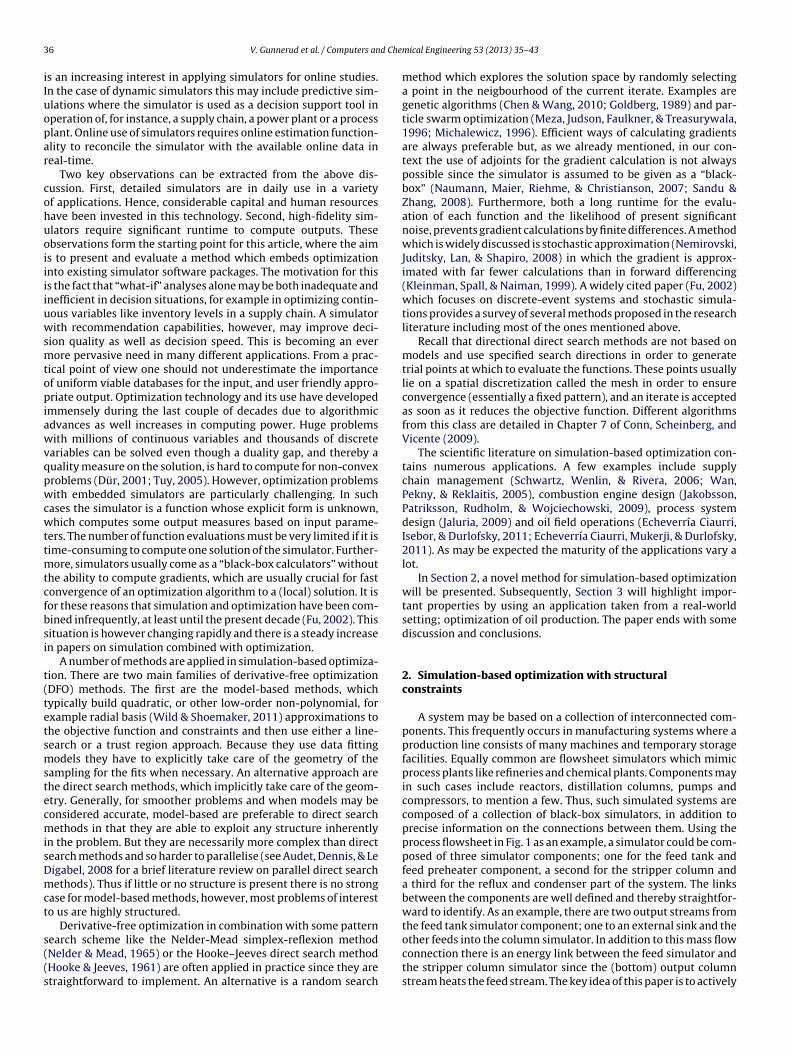

3 d Che

iIuopar

cohuoiiiiuwsmtopiawvqpwcwttmtcfbsi

t(tetsmstecmisDmct

s((s

6 V. Gunnerud et al. / Computers an

s an increasing interest in applying simulators for online studies.n the case of dynamic simulators this may include predictive sim-lations where the simulator is used as a decision support tool inperation of, for instance, a supply chain, a power plant or a processlant. Online use of simulators requires online estimation function-lity to reconcile the simulator with the available online data ineal-time.

Two key observations can be extracted from the above dis-ussion. First, detailed simulators are in daily use in a varietyf applications. Hence, considerable capital and human resourcesave been invested in this technology. Second, high-fidelity sim-lators require significant runtime to compute outputs. Thesebservations form the starting point for this article, where the aims to present and evaluate a method which embeds optimizationnto existing simulator software packages. The motivation for thiss the fact that “what-if” analyses alone may be both inadequate andnefficient in decision situations, for example in optimizing contin-ous variables like inventory levels in a supply chain. A simulatorith recommendation capabilities, however, may improve deci-

ion quality as well as decision speed. This is becoming an everore pervasive need in many different applications. From a prac-

ical point of view one should not underestimate the importancef uniform viable databases for the input, and user friendly appro-riate output. Optimization technology and its use have developed

mmensely during the last couple of decades due to algorithmicdvances as well increases in computing power. Huge problemsith millions of continuous variables and thousands of discrete

ariables can be solved even though a duality gap, and thereby auality measure on the solution, is hard to compute for non-convexroblems (Dür, 2001; Tuy, 2005). However, optimization problemsith embedded simulators are particularly challenging. In such

ases the simulator is a function whose explicit form is unknown,hich computes some output measures based on input parame-

ers. The number of function evaluations must be very limited if it isime-consuming to compute one solution of the simulator. Further-

ore, simulators usually come as a “black-box calculators” withouthe ability to compute gradients, which are usually crucial for fastonvergence of an optimization algorithm to a (local) solution. It isor these reasons that simulation and optimization have been com-ined infrequently, at least until the present decade (Fu, 2002). Thisituation is however changing rapidly and there is a steady increasen papers on simulation combined with optimization.

A number of methods are applied in simulation-based optimiza-ion. There are two main families of derivative-free optimizationDFO) methods. The first are the model-based methods, whichypically build quadratic, or other low-order non-polynomial, forxample radial basis (Wild & Shoemaker, 2011) approximations tohe objective function and constraints and then use either a line-earch or a trust region approach. Because they use data fittingodels they have to explicitly take care of the geometry of the

ampling for the fits when necessary. An alternative approach arehe direct search methods, which implicitly take care of the geom-try. Generally, for smoother problems and when models may beonsidered accurate, model-based are preferable to direct searchethods in that they are able to exploit any structure inherently

n the problem. But they are necessarily more complex than directearch methods and so harder to parallelise (see Audet, Dennis, & Leigabel, 2008 for a brief literature review on parallel direct searchethods). Thus if little or no structure is present there is no strong

ase for model-based methods, however, most problems of interesto us are highly structured.

Derivative-free optimization in combination with some pattern

earch scheme like the Nelder-Mead simplex-reflexion methodNelder & Mead, 1965) or the Hooke–Jeeves direct search methodHooke & Jeeves, 1961) are often applied in practice since they aretraightforward to implement. An alternative is a random search

mical Engineering 53 (2013) 35– 43

method which explores the solution space by randomly selectinga point in the neigbourhood of the current iterate. Examples aregenetic algorithms (Chen & Wang, 2010; Goldberg, 1989) and par-ticle swarm optimization (Meza, Judson, Faulkner, & Treasurywala,1996; Michalewicz, 1996). Efficient ways of calculating gradientsare always preferable but, as we already mentioned, in our con-text the use of adjoints for the gradient calculation is not alwayspossible since the simulator is assumed to be given as a “black-box” (Naumann, Maier, Riehme, & Christianson, 2007; Sandu &Zhang, 2008). Furthermore, both a long runtime for the evalu-ation of each function and the likelihood of present significantnoise, prevents gradient calculations by finite differences. A methodwhich is widely discussed is stochastic approximation (Nemirovski,Juditsky, Lan, & Shapiro, 2008) in which the gradient is approx-imated with far fewer calculations than in forward differencing(Kleinman, Spall, & Naiman, 1999). A widely cited paper (Fu, 2002)which focuses on discrete-event systems and stochastic simula-tions provides a survey of several methods proposed in the researchliterature including most of the ones mentioned above.

Recall that directional direct search methods are not based onmodels and use specified search directions in order to generatetrial points at which to evaluate the functions. These points usuallylie on a spatial discretization called the mesh in order to ensureconvergence (essentially a fixed pattern), and an iterate is acceptedas soon as it reduces the objective function. Different algorithmsfrom this class are detailed in Chapter 7 of Conn, Scheinberg, andVicente (2009).

The scientific literature on simulation-based optimization con-tains numerous applications. A few examples include supplychain management (Schwartz, Wenlin, & Rivera, 2006; Wan,Pekny, & Reklaitis, 2005), combustion engine design (Jakobsson,Patriksson, Rudholm, & Wojciechowski, 2009), process systemdesign (Jaluria, 2009) and oil field operations (Echeverría Ciaurri,Isebor, & Durlofsky, 2011; Echeverría Ciaurri, Mukerji, & Durlofsky,2011). As may be expected the maturity of the applications vary alot.

In Section 2, a novel method for simulation-based optimizationwill be presented. Subsequently, Section 3 will highlight impor-tant properties by using an application taken from a real-worldsetting; optimization of oil production. The paper ends with somediscussion and conclusions.

2. Simulation-based optimization with structuralconstraints

A system may be based on a collection of interconnected com-ponents. This frequently occurs in manufacturing systems where aproduction line consists of many machines and temporary storagefacilities. Equally common are flowsheet simulators which mimicprocess plants like refineries and chemical plants. Components mayin such cases include reactors, distillation columns, pumps andcompressors, to mention a few. Thus, such simulated systems arecomposed of a collection of black-box simulators, in addition toprecise information on the connections between them. Using theprocess flowsheet in Fig. 1 as an example, a simulator could be com-posed of three simulator components; one for the feed tank andfeed preheater component, a second for the stripper column anda third for the reflux and condenser part of the system. The linksbetween the components are well defined and thereby straightfor-ward to identify. As an example, there are two output streams fromthe feed tank simulator component; one to an external sink and the

other feeds into the column simulator. In addition to this mass flowconnection there is an energy link between the feed simulator andthe stripper column simulator since the (bottom) output columnstream heats the feed stream. The key idea of this paper is to actively

d Chem

toamstot

slthsp

2

cEoFaeaays

A

0, i.e

, MN

an d+1

work

tion

imulki )|

s acc

close

tIiern

V. Gunnerud et al. / Computers an

ake advantage of structural information to improve the efficiencyf simulation-based optimization. This will be done by designingn optimization scheme which combines simulation-based opti-ization on a component level with structural information. The

tructural information will be included as constraints. Returning tohe example in Fig. 1, one obvious constraint would be that ‘theutput (mass) flow-rate from the feed tank simulator must equalhe column feed flow-rate’.

The method is applicable to simulators which are composed ofeveral simulator components. Other types of complex simulators,ike a large reservoir model for a petroleum asset which may con-ain millions of model equations (Jansen et al., 2008) or a detailedeat distribution model of a reactor, which only contain one (huge)imulator component, will hence not benefit directly from the pro-osed approach.

.1. Method

The proposed method will now be described for a system with Nonnected components which are described by one simulator each.ach simulator depends on local continuous and binary variablesnly, i.e. S1(x1, y1), . . ., SN(xN, yN) where xi ∈ R

ni and yi ∈ {0, 1}mi .urther, the N simulators are linked by a set of constraints c(x, y) ≥ 0,nd x is bounded, i.e. x ≤ x ≤ x. There exists one proxy models forach simulator; M1(x1, y1), . . ., MN(xN, yN). Finally, xT = (xT

1, . . . , xTN)

nd yT = (yT1, . . . , yT

N). Hence, the complete simulator may be givens {S(x, y) subject to c(x, y) ≥ 0} with S(x, y) = {S1(x1, y1), . . ., SN(xN,N)}. The proposed algorithm is presented in Algorithm 1. Super-cript k defines the algorithm iteration number.

lgorithm 1 (Simulator optimization.).

Choose an initia l value for xk, yk, k =

Generat e proxy models M1(x01, y

01), ...

repeatAssemble th e optimization problempackage, i.e. compute xk+1 and yk

Set k = k + 1 an d establis h a new solution found in th e pr evoiu s step

Run al l simulators fo r th e new solu

for i = 1, ..., N doCompute th e gap between th e s gapi = |Si(xk

i , yki ) − Mi(xk

i , y

if gapi < th reshold thenProxy model Mi(xk

i , yki ) ha

elseRun Si for di fferen t values

endend

untilall gapi < th reshold;

Several comments are appropriate at this stage. A basic assump-ion is the fact that each simulator Si uses local variables only.n practice one variable may be shared by two simulators. This

s handled by the linking constraints through a simple (linear)quality. The proxy models Mi may take on many different formsanging from linear or nonlinear polynomial models to neuraletworks or operators with some appropriate bases. There is

ical Engineering 53 (2013) 35– 43 37

. th e initia l operatio n point

(x0N , y0

N ) fo r eac h simulator Si at x0, y0

sol ve it with an appropriat e optimization

ing point xk, yk, usin g th e optimal

S1(xk1, y

k1 ), ... , SN (xk

N , ykN )

ators an d th e prox y models

eptabl e qualit y an d is kep t unchanged

to xki , y

ki , to modify Mi

typically a trade-off between the number of required calculationsof Si and the approximation accuracy of Mi. Each proxy model willapply within a trust region, i.e. a closed ball centered at (xk

i, yk

i) in

which the model Mi is meant to be a valid approximation of Si.Two key issues are how to update the proxy models and their

corresponding trust regions. There are many options and twoparticular choices will be presented in conjunction with the oil pro-duction optimization case in the next section. A couple of generalcomments can however be made. The trust region of each proxymodel will determine the maximum allowable distance betweenthe current iterate (xk, yk) and the following (xk+1, yk+1). Hence, itdoes not make sense to ignore all earlier simulated points whenupdating a model Mi . A plausible strategy is to remove one dis-tant simulation point and add one new one by computing Si for onenew point. Further, it is only necessary to update the proxy modelswhich violate some predetermined accuracy measure since someof the proxy models may be more accurate than others. The adjust-ment of the trust regions for each model needs some care. Theyneed to be balanced since the accuracy of the different proxy mod-els are typically not uniform, and they are not only viewed as a localproperty. To elaborate, when one considers separate trust regionmodels and radii for the subproblems considered here then oneneeds to reconcile them by considering some compatible overallmodel that links, for example the separate trust regions with someoverall measure of trust. Similarly one needs an overall model tomeasure overall progress. There is also the concept of relativelynegligible terms. Details in the particular case of partially separa-ble decompositions (which includes the truly separable, as here)are given in Conn, Gould, and Toint (1996).

Any suitable optimization package which implements a trustregion method can be used. In the general case a MINLP solver isnecessary while continuous problems may apply nonlinear solvers

like IPOPT or SNOPT. In the later case we use the MINLP solverBONMIN.

To re-iterate the complete system is described by simulatorsS1(x1, y1), . . ., SN(xN, yN) and connection between them c(x, y) ≥ 0.

38 V. Gunnerud et al. / Computers and Chemical Engineering 53 (2013) 35– 43

FROMEVAPOR ATOR

PLANT

FEE DTANK

REFLUXTANK

TO HOTWATERTANK

FROM FOULWATER TANK

GASTOINCINERATOR

REFLUXCOND ENSER

WARMWATER

COO LWATER

COND ENSER

FEE DPREHEATER

STRIPP INGSTEAM

STRIPP ERCOLUMN

proce

Tptmta

aup

3

itswclbttmbpdasoi

ocm

Fig. 1. Example of a

his work assumes that the links c are linear and that they are incor-orated explicitly. More generally, the fact that they are analytic ishe essential ingredient. This makes sense since the links describe

ass and energy links, or help to split a common variable into intowo local variables through an equality constraints as discussedbove.

Later, in conjunction with the case which will be studied below more detailed algorithm will be presented. It will include partic-lars on the choice of proxy models, model updating, optimizationackage, initialization and termination criteria.

. Case example – optimization of oil production

Although appropriate for a wide class of applications thentended use of the proposed method is for production optimiza-ion in oil and gas operations. Production optimization coverstrategies for closed loop control, i.e. automated as far as is possible,hich would integrate both fast decision loops (surface facilities,

onsisting of, for example, process plants and pipelines) and slowoops linked to the subsurface reservoir, as well as the interactionetween the two (Foss, 2012). Currently for very complex sys-ems one relies to a significant extent on human intervention andhe optimization is carried out on disconnected (from a mathe-

atical point of view) subproblems. Consequently, any results cane significantly suboptimal, independently of how well the (sub)-roblems perform and independently of how well the optimizationoes. In reality of course, the models are sometimes very crudepproximations and the optimization is also more likely to be aignificant improvement rather than a good approximation to theptimum. Nevertheless, in this realistic environment we aim tontegrate and approximate as well as it is possible, such an optima.

To test the properties and potential of the proposed methodol-gy an example inspired by offshore oil and gas fields is used. Theontrol variables are the opening of choke valves, and the align-ent of production wells for the different trains of production. The

ss plant flowsheet.

constraints include the treatment capacity of gas and water, andthe bounds on the pressure in the lines and manifolds.

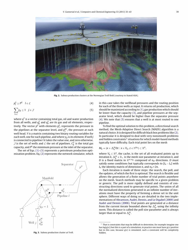
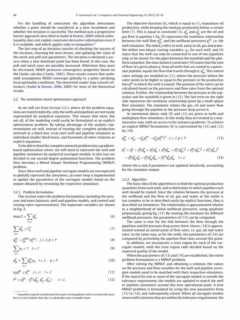
Production wells are typically organized in subsea clusters asshown Fig. 2. The subsea production clusters at Troll, which areshown in Fig. 2, consist of one, two or three manifolds, and fromthree to ten wells. All clusters have two parallel pipelines that con-nect the wells to the platform process facility. In this work a threewell one manifold cluster is considered. A layout of such a clusteris illustrated in Fig. 3.

In practice the operator would like to maximize the oil pro-duction while keeping the gas production below a certain limit,which entails finding the production quantities from each well, anddetermining to which pipeline the results should be routed.

There exists several simulators for oil and gas productionsystems. They include FlowManager from FMC, K-SPICE fromKongsberg Oil and Gas, GAP from Petroleum Experts, OLGA fromSPT Group, PipeSim from Schlumberger and PEX from Weatherford.In the following two sections the production optimization problemis presented and discussed according to two solution approaches,applying a derivative free method viewing the system as one largeproblem or using the simulation-based optimization method pro-posed in Section 2. Some details are omitted since the problem isthoroughly described in an earlier publication on Dantzig Wolfedecomposition and piecewise linearization through SOS2 sets inGunnerud and Foss (2010).

3.1. Derivative free optimization

The optimization problem corresponding to the production net-work shown in Fig. 3 can be represented by:

max Z = qTo (1)

s.t.

qT , pS = f (pW , Y)(2)

qTg ≤ CT

g (3)

V. Gunnerud et al. / Computers and Chemical Engineering 53 (2013) 35– 43 39

Norwe

p

∑

wfttweiJc

m

Fig. 2. Subsea production clusters at the

Sl ≥ PS l ∈ L (4)

l∈Lyjl ≤ 1 j ∈ J (5)

here qT is a vector containing total gas, oil and water productionrom all wells, and qT

g and qTo are its gas and oil elements, respec-

ively. The vector pS with elements pSl, represents the pressure in

he pipelines at the separator level, and pWj

, the pressure at eachell head. Y is a matrix containing two binary routing variables for

ach well, one for each pipeline, and where yjl is its element. If well js connected to pipeline l it takes the value one, and zero otherwise.

T

is the set of wells and L the set of pipelines. Cg is the total gasapacity, and PS the minimum pressure at the inlet of the separator.

The set of Eqs. (1)–(5) represents a petroleum production opti-ization problem. Eq. (2) represents the network simulator, which

Fig. 3. Subsea production cluster at Troll.

gian Troll field (courtesy to Statoil ASA).

in this case takes the wellhead pressures and the routing positionfor each of the three wells as input. It returns oil production, whichshould be maximized according to (1), gas production which shouldbe lower than the capacity (3), and pipeline pressures at the sep-arator level, which should be higher than the separator pressure(4). We note that (5) ensures that a well is at most routed to onepipeline.

To find the optimal solution to this problem, a directional searchmethod, the Mesh-Adaptive Direct Search (MADS) algorithm is anatural choice. It is designed for difficult black box problems like (2).In particular it is designed to deal with very nonsmooth problemsand hidden constraints1 situations for which model-based methodstypically have difficulty. Each trial point lies on the mesh

Mk = {x + �mk Dz : x ∈ Vk, z ∈ N

nD } ⊂ Rn,

where Vk ⊂ Rn, the cache, is the set of all evaluated points up to

iteration k, �mk

∈ R+ is the mesh size parameter at iteration k, andD is a fixed matrix in R

n×nD composed of nD directions. D mustsatisfy some conditions but typically corresponds to [In − In] withIn the identity matrix of dimension n, and nD = 2n.

Each iteration is made of three steps: the search, the poll, andthe updates, of which the first is optional. The search is flexible andallows the generation of a finite number of trial points anywhereon the mesh. Search methods may be specific to a given problemor generic. The poll is more rigidly defined and consists of con-structing directions used to generate trial points. The union of allthe normalized directions generated in an infinite number of iter-ations must have the property of forming a dense set in the unitsphere. Different ways of doing so are detailed in the two imple-mentations of Abramson, Audet, Dennis, and Le Digabel (2009) andAudet and Dennis (2006). Trial points are generated at a distance

from the current iterate bounded above by �p

k, using the infinity

norm. This distance is called the poll size parameter and is alwayslarger than or equal to �m

k.

1 That is constraints that may be difficult to determine, for example imagine onehas log(g(x)) but this is a part of a simulation, in practice one must have g(x) positivebut in this case, because g(x) is simulated, such a constraint will be completelyhidden.

4 d Che

wwbti

ttcpbtmler

3

trnornie

bpdtp

tto

3

sri

m

∑

q

∑

q

y

P

b

0 V. Gunnerud et al. / Computers an

For the handling of constraints the algorithm determineshether a point should be considered as a new incumbent andhether the iteration is successful. The method uses a progressive

arrier approach (described in Audet & Dennis, 2009) which unfor-unately does not exploit constraint derivative information even ift is available, and which applies only to inequalities.2

The last step of an iteration consists of checking the success ofhe iteration, choosing the next iterate, and updating the value ofhe mesh and poll size parameters. The iteration is declared a suc-ess when a new dominant point has been found. In this case, theoll and mesh sizes are possibly increased. Otherwise they muste decreased. MADS possesses convergence properties based onhe Clarke calculus (Clarke, 1983). These results ensure that under

ild assumptions MADS converges globally to a point satisfyingocal optimality conditions. The interested reader may consult ref-rences (Audet & Dennis, 2006, 2009) for most of the theoreticalesults.

.2. The simulation-based optimization approach

As we will see from Section 3.2.1, where all the problem equa-ions are stated explicitly, only the wells and pipelines are not easilyepresented by analytical equations. This means that most, butot all, of the modeling could easily be formulated as an explicitptimization problem. By taking advantage of the analytic rep-esentation we will, instead of treating the complete productionetwork as a black box, treat each well and pipeline simulator as

ndividual smaller black boxes, and formulate all other relations asxplicit equations.

To be able to feed the complete network problem into a gradient-ased optimization solver, we will need to represent the well andipeline simulators by analytical surrogate models. In this case weecided to use second degree polynomial functions. The problemhen becomes a Mixed Integer Nonlinear Programming (MINLP)roblem.

Since these well and pipeline surrogate models are not expectedo globally represent the simulators, an outer loop is implementedo update the parameters of the surrogate models based on theutput obtained by rerunning the respective simulators.

.2.1. Problem formulationThis section states the problem formulation, including the pres-

ure and mass balances, well and pipeline models, and control andouting valve representations. The important variables are shownn Fig. 3.

ax Z =∑

l∈LqP

lo (6)

l∈LqP

lg ≤ CTg (7)

Wjp = f WPC

jp (pWj ) j ∈ J, p ∈ P (8)

l∈Lyjl ≤ 1 j ∈ J (9)

Plp =

∑

j∈JqW

jp yjl l ∈ L, p ∈ P (10)

M W

jlpl ≤ pj j ∈ J, l ∈ L (11)

S = pMl − f P

l (qPlg, qP

lo, qPlw) l ∈ L (12)

2 Equalities may be transformed into pairs of inequalities with a certain tolerance,ut it is not evident that this is a desirable way to handle them.

mical Engineering 53 (2013) 35– 43

The objective function (6), which is equal to (1), maximizes oilproduction, while keeping the total gas production below a certainlimit (7). This is equal to constraint (3). qP

loand qP

lgare the oil and

gas flow in pipeline l. Eq. (8) represents the nonlinear relationshipbetween the well flow qW

jp, and the wellhead pressures pW

j, i.e. the

well simulator. The index j refers to well, and p to oil, gas and water.We define two binary routing variables, yjl, for each well, and (9)states that the well can only be connected to one of two pipelinesonly, or be closed. For the pipes between the manifold and the plat-form separator, the mass balance constraint (10) states that the sumof flow of a given phase p, from all wells that are routed to a partic-ular pipeline, equals the flow that travels through it, qP

lp. The control

valve settings are modeled in (11), where the pressure before thevalve needs to be higher or equal to the pressure in the productionline pM

lto which the well is routed. The position of the valve can be

calculated based on the pressures and flow rates from the optimalsolution. Further, the relationship between the pressure at the sep-arator and the manifold is given in (12). The last term on the rightside represents the nonlinear relationship given by a multi-phaseflow simulator. The simulator relates the gas, oil and water flowgoing through the pipeline to the pressure drop across it.

As mentioned above, only (8) and (12) are given as wells andmultiphase flow simulators. In this study they are treated in a non-inovasive way, with no access to for instance gradients. To achievean explicit MINLP formulation (8) is represented by (13) and (12)by (14).

qWjp = ˛1

jp − ˛2jppW

j − ˛3jp(pW

j )2 j ∈ J, p ∈ P (13)

pPl = ˇ1

l + ˇ2l qP

lg + ˇ3l qP

lo + ˇ4l qP

lw + ˇ5l (qP

lg)2 + ˇ6l (qP

lo)2 + ˇ7l (qP

lw)2

+ ˇ8l qP

lgqPlo + ˇ9

l qPlgqP

lw + ˇ10l qP

loqPlw l ∈ L (14)

where the ̨ and ̌ parameters are updated iteratively, accountingfor the simulator output.

3.2.2. AlgorithmThe basic idea of the algorithm is to find the optimal production

quantities from each well, and to determine to which pipeline eachwell should be routed. Since the relation between the pressure atthe wellhead and the flow of oil, gas and water at the outlet istoo complex to be to described easily by explicit functions, they isdescribed via simulators. The relationship is approximated relativeto a neighborhood of initial wellhead pressures, using quadraticpolynomials, giving Eq. (13). By running the simulator for differentwellhead pressures, the parameters of (13) can be computed.

The same is true for the link between the flow through thepipelines and the pressure drop across them. Hence, (14) is approx-imated around an initial point of flow rates, i.e. gas, oil and waterrates. In the same way, as for the wells, the parameters of (14) arecomputed by perturbing the pipeline flow rates around this point.

In addition, we incorporate a trust region for each of the sur-rogate models, with the trust region radii decided based on theexpected quality of the model.

When the parameters of (13) and (14) are established, the entireproblem formulation is a MINLP problem.

After solving the MINLP, and obtaining a solution, the valueson the pressure and flow variables for the well and pipeline surro-gate models need to be matched with their respective simulators.If the match for one or more of the surrogate models is outside thetolerance requirement, the models are updated to match the well

or pipeline simulators around this new operational point. A newMINLP problem is formulated by using the new parameters from(13) to (14), and subsequently solved. When all surrogate modelsreturn with solutions that are within the tolerance requirement, the

d Chem

oT

A

and fl

s clo ose t

least

optim

tion

to xk

lose t

4

dFmtlaa

ibN

pTha

to the network simulator. Subsequently, the network simulatorreturns oil production, i.e. the objective function value, gas pro-duction, which should be compared with total gas capacity, and

Table 1Results from computational study.

Algorithm Black box With structuralconstraints

V. Gunnerud et al. / Computers an

ptimization procedure terminates with a locally optimal solution.he algorithm is shown in more detail as Algorithm 2.

lgorithm 2 (Petroleum production simulator optimization.).

Choose an initia l point xk,yk, k = 0. Note that x contai n pressur e while y contains routing variables.

Run well simulator j for n1 (e.g. 5-10) di fferent wellhea d pressure Run pipelin e simulator l for n2 (e.g. 30-500) di fferen t flow rate s cl

Compute α and β parameter s to establis h (13 ) an d (14 ) by usin g a

repeatMINLP is established an d sol ved

Set k = k + 1 an d establis h new workin g point xk, yk, i.e. th efound by BONM IN

Run th e well simulators (8 ) with wellhea d pressures xk

Run th e pipelin e simulato r (12) wit h flow rates xk

Compute th e gap between th e simulato r resul t an d MINL P solu foral l the wells do j: |(8) - (13)| = gapj

foral l the pipelines do l: |(12) - (14)| = gapl

foral l the sur rogat e models doif if gap < th reshold thenSurrogat e mode l is OK

elseif well model thenRun well simulator for n1 differen t pressure s clos e Compute α parameter s to establis h (13)

end

if pipeline model thenRun pipelin e simulato r for n2 differen t flow rate s c Compute β parameter s to establis h (14)

endend

enduntil all sur rogat e model s are OK ;

. Computational study and results

The computational studies performed on the case example wereone with the two approaches presented in the previous section.irst, the network simulator was treated as one simulator, and opti-ized with a “standard” black box approach. This will be referred

o as the baseline case. In the second approach, the network simu-ator was split into pieces and the network structure was includeds explicit constraints. The results from both computational studiesre presented in Table 1.

To establish the baseline results, the network simulator wasmplemented in Matlab, and a Matlab version of the NOMAD blackox optimization software NOMAD, 2011, i.e. NOMADm, was used.OMAD is an advanced implementation of the MADS algorithm.

However, the well and pipeline simulators are still compiled

roprietary code, respectively from Statoil and Petroleum Experts.o bypass interface coding and thereby ease the implementation,igh resolution tables were generated upfront. Note that the resultsnd following discussion is based on the computations needed as

ical Engineering 53 (2013) 35– 43 41

ow rates

se to x0, y0

o x0, y0

squar e fit

al solution

for xk, yk

o xk

if the simulators would be integrated with the optimization algo-rithm, i.e. the work of creating these high resolution tables is notincluded in the computational study. The Matlab network simula-tor used data from these tables instead of running the simulatorswithin the optimization loop. The NOMADm optimization algo-rithm suggested well head pressures and routings for each well

Algorithm iterations 351 4Well simulations 23,402 82Pipeline simulations 15,602 1662Normalized oil production 0.90 1

4 d Che

pcfiit

dMmhgwempstrAafbom

natftt7aa

hdavoms

5

sscegucpnisnctfilSl

2 V. Gunnerud et al. / Computers an

ressure on each pipeline at the inlet separator, which should beompared with the separator pressure. The solution is consideredeasible if the gas rate is below the capacity level, and the pressuren each line at the separator level is above the separator pressure,.e. the gas and pressures are treated as variables with bounds byhe NOMADm algorithm.

The implementation of the method proposed in this paper wasone in C++, within the framework of COIN-OR (2011), and theINLP problem is solved by BONMIN. As for the Matlab imple-entation, the interface to the well and pipeline simulators were

andled through high resolution tables. To establish the well surro-ate model (13), simulations for seven different well head pressuresere run and a least squares fit was used to find the three param-

ters of the second degree polynomials. For the surrogate pipelineodels (14) which have ten parameters, seven simulations for each

hase i.e. oil, gas and water were run. This amounts to 7 × 7 ×7 = 343imulations runs. Also in this case, a least squares fit was used to findhe parameters of the second degree polynomials. A simple trustegion management approach is incorporated for the well models.

large trust region is used in the first two iterations (25 bar abovend below the working point), where one expects to be far awayrom the optimal solution, and a smaller one (10 bar above andelow the working point) comes into play from iteration three inrder to narrow down the search area. The rules of the trust regionanagement are based on experience from preliminary tests.Table 1 summarizes the results. Well simulations refer to the

umber of well simulations which had to be made. In the black boxpproach there were three well simulations per network simula-ion, while in the proposed method there were seven simulationsor each of the three wells. And similarly for the pipeline simula-ions, there were two for each black box network simulation, whilehere were two times 343 in the proposed method. This implies that802 complete black box network simulations were run to arrivet the answer. Simulation results from previous iterations of thelgorithm were reused.

In the black box approach, we were not able to make NOMADmandle the routing variables properly. The authors believe this isue to the severe nonlinearities, and the fact that all discrete vari-bles are binary so that a structured integer search does not workery well. The nine most promising routing alternatives (at leastne well open and symmetry were removed) were therefore triedanually, the best found solution was chosen, and the number of

imulations were summed up for these nine alternatives.

. Discussion

As we argue in Section 2, there are many applications whereimulators are structured in networks, and where these networkimulators easily can be broken down into smaller stand-aloneomponents. This is particularly true for process simulators. How-ver, the applicability of this optimization approach is quiteeneral. Value chain simulators typically consist of multiple sim-lators connected throughout the value chain. To provide someontext to this discussion section it is difficult to do a robust com-arison, even between two nonlinear programming algorithms,ever mind mixed integer nonlinear methods. Such a comparison,

f carefully done, is beyond the scope of the present article. The rea-ons for this are many. First of all there are very few mixed integeronlinear programming codes, and many of them (if not all) do notlaim to be robust. Some are designed to solve the global optimiza-ion problem and others are content to determine local optima. The

rst are really only suitable for relatively low dimensional prob-

ems and would certainly be inefficient when local optima suffice.econd, if only local optima are required competing algorithms areikely to converge to different local optima.

mical Engineering 53 (2013) 35– 43

The optimization approach is tested on a small but realisticpetroleum production problem, where the computational studyshows a significant improvement compared to a standard blackbox/noninvasive approach.

The solution quality in terms of oil production was improved bymore than 10%. This is a very large number in this context and willmost probably not hold in all applications. The number of pipelinesimulations was almost one magnitude lower, and the number ofwell simulations, more than two. In these applications a well sim-ulation could take 100 times more time than a pipeline simulation.This indicates that the solution time sees a speed up of two ordersof magnitude, and this is without exploring the option of solvingthe component simulators in parallel.

The method naturally splits the problem into smaller subprob-lems, in this case wells and pipelines. However, these wells andpipeline simulators are run many times in each of the algorithmiterations, and there is only the number of available CPUs whichprevents us from running all at the same time. In our case this wouldamount to 343 × 2 +7 × 3 =707 separate computations. Given thatthere were 707 CPUs available, the algorithm would only have towait for the slowest well calculation four times. In practice, how-ever, one would need much less, approximately 7 × 3 +7 = 28 CPUs,since the pipeline simulations could be run on 7 CPUs. The black boxalgorithm is also easily parallelized, but it cannot be parallelizedon a component level. Each network simulation will need to runthree well and two pipeline simulations, in a total of 351 sequentialiterations. If we do not consider the run time of the pipeline sim-ulator which is embedded inside the network simulator, a speedup of 4–1053 (351 × 3 =1053) could be expected. The black boxapproach runs 7802 network simulations distributed over 351 iter-ations which means that on average it will use 23 CPUs. However,some of the algorithm iterations are runing many more than 23 net-work simulations, and the algorithm would therefore easily benefitfrom having more than 100 CPUs.

One of the reasons for faster convergence is the fact that theproposed method searches using much smaller simulators than theblack box approach, i.e. it is more realistic to estimate first and sec-ond order gradients, or proxy’s, for a single well model, than forthe complete production network. An estimate of what will hap-pen to the well flow rate if the well head pressure is changed ismore predictable than the consequence for the complete produc-tion network if one changes the same well head pressure, or if onereroutes a well to another pipeline. When the characteristics of thewells and pipelines are approximated by second order polynomials,the resulting MINLP optimization problem is limited to 26 variables(6 binary and 20 continuous), and 27 constraints, and it is solvedin less than a second. This tells us, not surprisingly, that much isgained by including explicit structural constraints as much as pos-sible. Hence, we should be able to address problems with a muchhigher degree of freedom in terms of optimization variables.

However, there are some significant challenges related to theapproach. It is a more complex task to divide the network sim-ulator into components and to update proxy models for each ofthem, compared to a single noninvasive implementation. In thenoninvasive case, where a derivative free algorithm is used, or onlyone proxy model for the completed network simulator is used, it ismore and less straightforward to implement an optimization algo-rithm on top of the simulator. For the proposed approach, thereis a need for in-depth problem, simulator and optimization knowl-edge. The presented approach is also limited to network simulatorsthat are easily decomposed, meaning that applicability to dynamicsimulators where components are closely interconnected through

dynamic behavior is still an open research question.

Possible improvements of the algorithm lie in the integrationbetween the simulators and the optimization model and algo-rithm. In this paper, the simulators are run to establish a full MINLP

d Chem

p&uNnaaufiit

6

nbdipTfbo

A

aIWtr

R

A

A

A

A

C

C

C

C

V. Gunnerud et al. / Computers an

roblem. However, a better approach could be to handle the branch bound part on top, and then for each NLP, run the necessary sim-lations. If a nonlinear interior point algorithm is used to solve theLP problem, the simulators could be used to generate any suitableonlinear constraint that could be handled by the interior pointlgorithm. On the other hand, if a sequential linear problem (SLP)lgorithm is used, it would be interesting to iterate using the sim-lators on the LP layer, to generate linear constraints and objectiveunction. By handling the interaction with the simulators below thenteger layer in the optimization algorithm, it will bypass possiblenstabilities due to major shifts in values, e.g. if a well is rerouted,he flows in the pipelines changes drastically.

. Conclusions

In this paper we have presented an algorithm that explores theatural structure of a network simulator, to find the best possi-le simulator settings given a predefined objective. The method isemonstrated on a realistic petroleum production problem where

t shows a speed up of more than two orders of magnitude, com-ared to a standard approach. The solution quality is also improved.he authors believe the advantages of the approach will improveurther, as the size of the network grows. Potentially, it shoulde possible to handle problem instances with 10–100 times moreptimization variables, than what is possible today.

cknowledgements

We acknowledge the support of the Center for Integrated Oper-tions at NTNU, Norway including their industrial sponsors, andBM for granting the Open Collaborative Research (OCR) award –

1055486. We also acknowledge Sheri Shamlou, for implemen-ing the algorithms, and for running the tests and generating theesults.

eferences

bramson, M. A., Audet, C., Dennis, J. E., Jr., & Le Digabel, S. (2009). OrthoMADS. Adeterministic MADS instance with orthogonal directions. SIAM Journal on Opti-mization, 20(2), 948–966.

udet, C., & Dennis, J. E., Jr. (2006). Mesh adaptive direct search algo-rithms for constrained optimization. SIAM Journal on Optimization, 17(1),188–217.

udet, C., & Dennis, J. E., Jr. (2009). A progressive barrier for derivative-free nonlinearprogramming. SIAM Journal on Optimization, 20(4), 445–472.

udet, C., Dennis, J. E., Jr., & Le Digabel, S. (2008). Parallel space decomposition ofthe mesh adaptive direct search algorithm. SIAM Journal on Optimization, 19(3),1150–1170.

hen, X., & Wang, N. (2010). Optimization of short-time gasoline blending sched-uling problem with a DNA based hybrid genetic algorithm. Chemical Engineeringand Processing: Process Intensification, 49(10), 1076–1083.

heng, X., & Jaluria, Y. (2005). Optimization of a thermal manufacturing process:Drawing of optical fibers. International Journal of Heat and Mass Transfer, 48(17),3560–3573.

larke, F. H. (1983). Optimization and nonsmooth analysis. New York: Wiley. Reissuedin 1990 by SIAM Publications, Philadelphia, as vol. 5 in the series Classics inApplied Mathematics.

OIN-OR. (2011). Computational infrastructure for operations research.http://www.coin-or.org/03.01.2011

ical Engineering 53 (2013) 35– 43 43

Conn, A. R., Deleris, L. A., Hosking, J. R. M., & Thorstensen, T. A. (2010). A simulationmodel for improving the maintenance of high cost systems, with application toan offshore oil installation. Quality and Reliability Engineering International, 73,3–748.

Conn, A. R., Gould, N., & Toint, P. L. (1996). Convergence properties of minimizationalgorithms for convex constraints using a structured trust region. SIAM Journalon Optimization, 6, 1059–1086.

Conn, A. R., Scheinberg, K., & Vicente, L. N. (2009). Introduction to derivative-freeoptimization. MPS/SIAM book series on optimization. Philadelphia: SIAM.

Dür, M. (2001). Dual bounding procedures lead to convergent branch-and-boundalgorithms. Mathematical Programming Series A, 91, 117–125.

Echeverría Ciaurri, D., Isebor, O. J., & Durlofsky, L. J. (2011). Application ofderivative-free methodologies to generally constrained oil production optimi-sation problems. International Journal of Mathematical Modelling and NumericalOptimisation, 2, 134–161.

Echeverría Ciaurri, D., Mukerji, T., & Durlofsky, L. J. (2011). Derivative-free opti-mization for oil field operations. In X.-S. Yang, & S. Koziel (Eds.), Computationaloptimization and applications. Berlin Heidelberg: Springer-Verlag.

Foss, B. (2012). Process control in conventional oil and gas field – Challenges andopportunities. Control Engineering Practice, 20, 1058–1064.

Fu, M. C. (2002). Optimization for simulation: Theory vs. practice. INFORMS Journalof Computing, 192–215.

Goldberg, D. E. (1989). Genetic algorithms in search, optimization and machine learning.Boston: Addison-Wesley Longman.

Gunnerud, V., & Foss, B. (2010). Oil production optimization – A piecewise lin-ear model, solved with two decomposition strategies. Computers & ChemicalEngineering Journal, 34, 1803–1812.

Hooke, R., & Jeeves, T. A. (1961). ‘Direct search’ solution of numerical and statisticalproblems. Journal of the Association for Computing Machinery, 21, 2–229.

Jakobsson, S., Patriksson, M., Rudholm, J., & Wojciechowski, A. (2009). A methodfor simulation based optimization using radial basis functions. Optimization andEngineering, 11

Jaluria, Y. (2009). Simulation-based optimization of thermal systems. Applied Ther-mal Engineering, 29, 1346–1355.

Jansen, J. D., Bosgra, O. H., & Van den Hof, P. M. J. (2008). Model-based control ofmultiphase flow in subsurface oil reservoirs. Journal of Process Control, 18(9),846–855.

Kleinman, N. L., Spall, J. C., & Naiman, D. Q. (1999). Simulation-based optimiza-tion with stochastic approximation using common random numbers. INFORMSManagement Science.

Meza, J. C., Judson, R. S., Faulkner, T. R., & Treasurywala, A. M. (1996). A comparisonof a direct search method and a genetic algorithm for conformational searching.Journal of Computational Chemistry, 17(9), 1142–1151.

Michalewicz, Z. (1996). Genetic algorithms + data structures = evolution programs (3rded.). Berlin: Springer-Verlag.

Naevdal, G., Brouwer, D. R., & Jansen, J. D. (2006). Waterflooding using closed-loopcontrol. Computational Geosciences, 10, 37–60.

Naumann, U., Maier, M., Riehme, J., & Christianson, B. (2007). Automatic first- andsecond-order adjoints for truncated Newton.

Nelder, J. A., & Mead, R. (1965). A simplex method for function minimization. Com-puter Journal, 308–313.

Nemirovski, A., Juditsky, A., Lan, G., & Shapiro, A. (2008). Robust stochastic approx-imation approach to stochastic programming. SIAM Journal on Optimization,19(4), 1574–1609.

NOMAD. (2011). A blackbox optimization software. http://www.gerad.ca/nomad/Project/Home.html/06.10.2011

Rutenbar, R. A., Gielen, G. G. E., & Antao, B. A. (Eds.). (2002). Computer-aided designof analog integrated circuits and systems. New York, USA: Wiley-IEEE Press.ISBN:047122782X

Sandu, A., & Zhang, L. (2008). Discrete second order adjoints in atmospheric chemicaltransport modeling. Journal of Computational Physics, 227(12), 5949–5983.

Schwartz, J. D., Wenlin, W., & Rivera, D. E. (2006). Simulation-based optimization ofprocess control policies for inventory management in supply chains. Automatica,42, 1311–1320.

Tuy, H. (2005). On solving nonconvex optimization problems by reducing the dualitygap. Journal of Global Optimization, 32, 349–365.

Wan, X., Pekny, J. F., & Reklaitis, G. V. (2005). Simulation based optimization withsurrogate models-application to supply chain management. Computers andChemical Engineering, 29, 1317–1328.

Wild, S. M., & Shoemaker, C. (2011). Global convergence of radial basis function trustregion derivative-free algorithms. SIAM Journal on Optimization, 21(3), 761–781.