Emanuel Parzen: A Memorial, and a Model With the TwoKernels That He Championed

Grace Wahba1

Department of Statistics, Department of Computer Sciencesand Department of Biostatistics and Medical Informatics

University of Wisconsin, MadisonMarch 16, 2018

Abstract

Manny Parzen passed away in February 2016, and this article iswritten partly as a memorial and appreciation. Manny made impor-tant contributions to several areas, but the two that influenced memost were his contributions to kernel density estimation and to Re-producing Kernel Hilbert Spaces, the two kernels of the title. Somefond memories of Manny as a PhD advisor begin this memorial, fol-lowed by a discussion of Manny’s influence on density estimation andRKHS methods. A picture gallery of trips comes next, followed by thetechnical part of the article. Here our goal is to show how risk modelscan be built using RKHS penalized likelihood methods where sub-jects have personal (sample) densities which can be used as attributesin such models.

1 Scholar, teacher, friend

1.1 Manny as PhD advisor

In 1962 I was a single mom working at a D. C. area think tank and alsoworking towards a Masters at the University of Maryland-College Park whenI read Mod Prob [19] and Stochastic Processes [24], and imagining an impos-sible dream of relocating to the West Coast, going to Stanford and having

1Research supported in part by NSF Grant DMS-1308847 and a Consortium of NIHInstitutes under Award Number U54AI117924

1

arX

iv:1

803.

0555

5v1

[st

at.O

T]

15

Mar

201

8

Prof. Emanuel Parzen as a thesis advisor. Well, sometimes dreams do cometrue. I got a new job with a group at IBM in D. C. and shortly thereafter,they moved the whole group to the Bay area. Voila, admission to the IBMwork study program and to Stanford and eventually I became Manny’s fifthstudent. Soon we were meeting regularly and he would enthusiastically listento my initial attempts at research. I have many fond memories of my fiveyears as a student (1962-66 and postdoc 1967). One of my first memories isan elegant dinner that Manny and his wife Carol threw for a group of stu-dents - convincing me that academic life was something to be desired. Carolwas always part of things, knowing many of Manny’s students and beingenthusiastic about their academic lives. Once I got through the first yearqualifier (at Stanford they had first and second year qualifiers) I didn’t reallyworry about making it through (sort of). Manny was always encouraging,and he was the most positive, outgoing and optimistic person I had evermet. Another fond memory is a class Manny taught and held on nice dayson the grass in front of the old Sequoia hall, later demolished and replacedby a more modern new Sequoia hall in 1998. Manny was one of the majorfigures in time series analysis and this class reflected his contributions tothe field at the time, one example being the fundamental paper [21]. It wasthe first time I heard him talk about Reproducing Kernel Hilbert Spaces [1],although he had published several papers utilizing them around that time,for example [20] [25]. In any case, some of his elegant approaches to RKHSremained dormant in my brain for a few years (more on that later) and Iwent on to write a dissertation on vector valued time series [35, 36] under hissupervision. Manny looked after his students. It turned out that E. J. (Ted)Hannan, in Canberra, Australia was one of Manny’s scientific correspondentsand was working on something similar to my thesis work. Manny sent himwhat was to become [36]. Recalling that in the 60’s it could take three weeksto get a package to Australia, it happened that Hannan sent Manny whatwas to become [7] and the manuscripts crossed in the mail - a bit differentthan instant communication around the world today. I think Manny hadwritten Hannan about my work along with sending the manuscript, and al-though Hannan’s paper ultimately was published several years before mine,he generously mentioned my work in his paper. I received the PhD in Juneof 1966 and, if memory serves, Manny took me and my Dad, who had comefrom New Jersey for the graduation, to lunch at the faculty club. I went onto spend a year as a postdoc with Manny. During that year he apparentlycontacted a number of his friends, including George Box at Madison, result-

2

ing in a large number of invitations to give a lecture, and, ultimately eightjob offers. The late 60’s were a good time to be looking for an academic job,as universities were growing to accommodate the children of the veteransreturning from the Second World War. The process was much simpler, too- Manny made a bunch of phone calls, I gave some talks, and eventually Igot a letter with a short paragraph saying something like “We would like tooffer you a position as an assistant professor with the academic year salaryof (say) $10,000. Please let us know by such-and-such a date whether youaccept”. Today the successful applicant will get a large packet with enoughrules and regulations to keep busy reading them for a week. Not to mentionthe application process whereby the potential hire is usually responding toa job posting, enters a large number of documents into an on line website,while the applicant’s references have to enter detailed information into an-other website. In September of 1967 I left sunny California for the frozenwinters of the Midwest, the University of Wisconsin-Madison, where therewas a powerful numerical analysis group and a fertile place to nurture theseeds of function estimation in RKHS.

1.2 Manny’s influence – density estimation

Manny had written a fundamental paper on density estimation [23] (moreon this in the technical section below) and being aware of this work ledme to write a bunch of papers on density estimation and spectral densityestimation, including [37] [38] [39] [43]. In the early seventies there was a lotof discussion about tuning nonparametric models of various kinds. Mannycontributed to this issue in the context of time series, in his CATS tuningcriteria [27], and in his influence on those around him, for example, the lastthree papers above.

1.3 Manny’s influence – RKHS

In 1967, when I arrived in Madison, there was a large group of staff and visi-tors working excitedly in numerical analysis and approximation theory. Theywere members of the Mathematics Research Center which was located in Stir-ling Hall, the building that was later blown up in August of 1970 in protestagainst the Vietnam war. I had a part time appointment there along withmy position in the Statistics Department. Leading researchers in approxi-mation theory and numerical analysis were there, including I. J. Schoenberg,

3

Carl deBoor, Larry Schumaker, Zuhair Nashed and others. There was muchinterest in splines, the first of which were invented by Schoenberg in the for-ties. Tea was served mid morning and mid afternoon accompanied by livelydiscussion.

In the midst of this creativity, that brain space holding memories of RKHSfrom Manny’s class perked up, and George Kimeldorf, who was a visitor tothe MRC at the time, and I together realized that we could derive Schoen-berg’s polynomial smoothing spline as an optimization problem in an RKHS,and moreover the abstract structure for doing that was highly generalizable.We went on to produce three papers together about RKHS [8] [9] [10], thislast paper giving a closed form expression for the solution to the penalizedlikelihood optimization problem, where the penalty is a square norm or semi-norm in an RKHS - the representer theorem. It was accepted within threeweeks, something that I never experienced again. RKHS methods seemed tooccupy a small niche until around 1996 when it became widely known thatthe Support Vector Machine (SVM), much appreciated by computer scien-tists for its classification prowess, could be obtained as the solution to anoptimization problem in an RKHS. More on this story can be found in [41]pp. 486–495. Lin et al [16] showed that the SVM was estimating the sign ofthe log odds ratio, and copious applications of RKHS methods are now partof computer scientists’ and statisticians’ toolkits.

2 Trips

In 1984, Hirotugu Akaike threw a fun conference in Tokyo focused mostlyaround a group that was interested in time series and other common interestsof Akaike and Manny. There were exciting sightseeing trips and social eventsalmost every evening. I’m sure things are different now, but the graciousladies of the office staff served us tea and little cakes on conference days.One evening when I surprisingly didn’t see anything on the schedule, one ofAkaike’s younger (and presumably single) colleagues asked me if he couldtake me out to dinner, and I was quite charmed. I didn’t stop to wonderwhere everyone else was, but some years later I decided that it must havebeen planned to allow the men to visit some place that didn’t expect womene. g. a geisha teahouse, but I’ll never know.

4

Figure 1 is a picture from the Tokyo trip.

Figure 1: Akaike Time Series Conference, Tokyo 1984. l. to r. Victor Solo,Manny, me, Wayne Fuller, Bill Cleveland, Bob Shumway, David Brillinger

5

In 1989 there was a swell sixtieth birthday party for Manny, includingscientific colleagues, Texas A&M bigwigs and Parzen family. Everyone hada ball, and Figure 2 is a scene from the party - there is Manny outgoing andsmiling as ever.

Figure 2: Manny’s 60th Birthday, 1989, College Station, TX. l. to r. DonYlvisaker, me, Joe Newton, Marcello Pagano, Randy Eubank, Manny, WillAlexander, Marvin Zelen, Scott Grimshaw

6

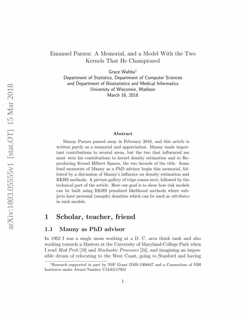
Marvin Zelen and I attended the JSM2005 Gottfried Noether ScholarsAward and are congratulating the winners, Manny and Gerda Claeskins, inFigure 3.

Figure 3: At the Gottfried Noether Senior and Junior Researchers AwardsCeremony, JSM 2005, to Manny Parzen and Gerda Claeskens. l. to r. me,Manny, Gerda, Marvin Zelen

7

Manny was the featured speaker at the The Pfizer Colloquium 2006 atUConn, with Joe Newton and myself as discussants. Joe and I sat for a“Conversation with Many Parzen”, (see Figure 4) which was videotaped,and the main thing I remember about that was the fact that the video wasrecording off the cuff remarks and I was afraid of making a dumb one. Mannyis smiling as usual but I look a bit tense.

Figure 4: Manny, me, Joe Newton, Nitis Mukhopadhyay at the Pfizer Collo-quium 2006 in Manny’s honor at UConn.

8

3 Manny, a man of many interests

Manny had a major role in a number of fundamental areas in the develop-ment of the Statistical Canon. Aside from density estimation and RKHS,these include time series modeling, spectral density estimation, and in lateryears, quantile estimation. However, in this chapter we will limit ourselves toParzen window density estimation and RKHS, two of Manny’s areas I haveworked in. Interestingly Manny’s work is fundamental to the two differentkinds of kernels that have played important roles in the development of mod-ern statistical methodology. Kernels in Parzen window density estimation (tobe called density kernels) are typically non-negative symmetric functions in-tegrating to 1 and satisfying some conditions, while kernels in RKHS arepositive definite functions, which are not necessarily positive. There are, ofcourse, kernels that are both. We will briefly review both, enough to reviewsome modern results in two emerging fields, density embedding and distancecorrelation. Density embedding begins with an RKHS and a sample froma density of interest and results in a class of density estimates which in-clude Parzen window estimates. These estimates are elements of the RKHSso one has a metric for determining pairwise distances between densities,namely the RKHS norm. This enlarges the class of familiar distance mea-sures between densities (e. g. Hellinger distance, Bhattacharyya distance,Wasserstein distance, etc.) Given pairwise distances between densities, wethen describe how these pairwise distances are used to include sample den-sities as attributes in statistical learning models such as Smoothing SplineANOVA (SS-ANOVA) models, which include penalized likelihood methodsand (nonparametric) SVM’s. Thus Manny’s foundational work in two seem-ingly diverse areas come together to add another feature to the statistician’stool kit.

3.1 Two kinds of kernels

We now discuss the two kinds of kernels, those used in density estimation, andthose that characterize an RKHS. Our goal is to show how sample densitiespossessed by subjects in RKHS-based prediction models can be treated asattributes in these models.

9

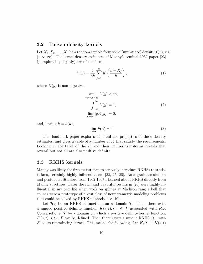
3.2 Parzen density kernels

LetX1, X2, . . . , Xn be a random sample from some (univariate) density f(x), x ∈(−∞,∞). The kernel density estimates of Manny’s seminal 1962 paper [23](paraphrasing slightly) are of the form

fn(x) =1

nh

n∑j=1

K

(x−Xj

h

), (1)

where K(y) is non-negative,

sup−∞<y<∞

K(y) <∞,∫ ∞−∞

K(y) = 1,

limy→∞|yK(y)| = 0,

(2)

and, letting h = h(n),limn→∞

h(n) = 0. (3)

This landmark paper explores in detail the properties of these densityestimates, and gives a table of a number of K that satisfy the requirements.Looking at the table of the K and their Fourier transforms reveals thatseveral but not all are also positive definite.

3.3 RKHS kernels

Manny was likely the first statistician to seriously introduce RKHSs to statis-ticians, certainly highly influential, see [22, 25, 26]. As a graduate studentand postdoc at Stanford from 1962-1967 I learned about RKHS directly fromManny’s lectures. Later the rich and beautiful results in [26] were highly in-fluential in my own life when work on splines at Madison rang a bell thatsplines were a prototype of a vast class of nonparametric modeling problemsthat could be solved by RKHS methods, see [10].

Let HK be an RKHS of functions on a domain T . Then there exista unique positive definite function K(s, t), s, t ∈ T associated with HK .Conversely, let T be a domain on which a positive definite kernel function,K(s, t), s, t ∈ T can be defined. Then there exists a unique RKHS HK withK as its reproducing kernel. This means the following: Let Ks(t) ≡ K(s, t)

10

be considered as a function of t for each fixed s. Then, letting < ·, · >be the inner product in HK , for f ∈ HK we have < f,Ks >= f(s), and< Ks, Kt >= K(s, t). The square distance between f and g is denoted as||f − g||2HK , where || · ||2HK is the square norm in HK . As a special case,if s, t ∈ T , then the squared distance between s and t can be taken as||Ks −Kt||2HK = K(s, s)− 2K(s, t) +K(t, t). We will be using the fact thatK encodes pairwise distances. We note that tensor sums and products ofpositive definite functions are positive definite functions and have associatedRKHS as tensor sums and products of the corresponding component RKHS,see [1] and the references cited below for examples.

3.4 Smoothing Spline ANOVA models

Basic references for SS-ANOVA models are [5] and [44], both describe soft-ware in the R collection. Numerous applications include [3, 15, 42]

Let T (α), α = 1, . . . , d be d domains with members tα ∈ T (α). Let

t = (t1, . . . , td) ∈ T (1) × · · · × T (d) = T .

With each domain we have a positive definite function and associated RKHS.Now let HK be the tensor product of the d RKHSs. Its RK is then thetensor product of the component RK’s. With some conditions, including thatthe constant function is in each component space and there is an averagingoperator in which the constant function averages to 1, then for f ∈ HK anANOVA decomposition of f of the form

f(t1, · · · , td) = µ+∑α

fα(tα) +∑αβ

fαβ(tα, tβ) + · · · (4)

can always be defined. Then a regularized kernel estimate is the solution tothe problem

minf∈HK

n∑i=1

C(y, f) + λJ(f), (5)

where C(y, f) relates to fit to predict y from f , for example a Gaussianor Bernoulli log likelihood, or a hinge function (Support Vector Machine),and J(f) is a square norm or seminorm in HK . Given this model for f(generally truncated as warranted) this provides a method for combining

11

heterogenous domains (attributes) in a regularized prediction model. Notethat nothing has been assumed about the domains, other than that a positivedefinite function can be defined on them. We sketch an outline of factsrelating to SS-ANOVA models, partly to set up notation to facilitate ourgoal of demonstrating how sample densities may be treated as attributes inconjunction with SS-ANOVA models.

The choice of kernel class for each variable may be an issue in practice andmay be specific to the particular issue and data at hand. Once the kernel formhas been chosen, the tuning parameter λ in Equation (4) along with othertuning parameters hidden in J(f) must be chosen and can be important.We are omitting any discussion of these issues here, but applications papersreferenced below discuss choice of tuning parameters.

Note that we use the same symbol K for density kernels, positive definitefunctions and positive definite matrices.

Let dµα be a probability measure on T (α) and define the averaging oper-ator Eα on T by

(Eαf)(t) =

∫T (α)

f(t1, . . . , td)dµα(tα). (6)

Then the identity operator can be decomposed as

I =∏α

(Eα + (I − Eα)) =∏α

Eα +∑α

(I − Eα)∏β 6=α

Eβ+

∑α<β

(I − Eα)(I − Eβ)∏γ 6=α,β

Eγ + · · ·+∏α

(I − Eα),

giving

µ = (∏α

Eα)f, fα = ((I − Eα)∏β 6=α

Eβ)f

fαβ = ((I − Eα)(I − Eβ)∏γ 6=α,β

Eγ)f . . .

Further details in the RKHS context may be found in [6, 40, 42]. Theidea behind SS-ANOVA is to construct an RKHS H of functions on T as thetensor product of RKHS on each T (α) that admit an ANOVA decomposition.Let H(α) be an RKHS of functions on T (α) with

∫T (α) fα(tα)dµα(tα) = 0

12

and let [1(α)] be the one dimensional space of constant functions on T (α).Construct the RKHS H as

H =d∏

α=1

([1(α)]⊕H(α))

= [1]⊕∑α

H(α) ⊕∑α<β

[H(α) ⊗H(β)]⊕ · · · , (7)

where [1] denotes the constant functions on T . Then fα ∈ H(α), fαβ ∈[H(α)⊗H(β)] and so forth, where the series will usually be truncated at somepoint. Note that the usual ANOVA side conditions hold here.

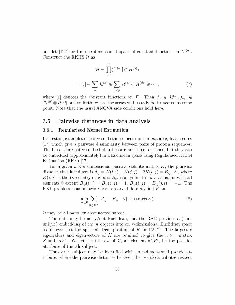
3.5 Pairwise distances in data analysis

3.5.1 Regularized Kernel Estimation

Interesting examples of pairwise distances occur in, for example, blast scores[17] which give a pairwise dissimilarity between pairs of protein sequences.The blast score pairwise dissimilarities are not a real distance, but they canbe embedded (approximately) in a Euclidean space using Regularized KernelEstimation (RKE) [17].

For a given n × n dimensional positive definite matrix K, the pairwisedistance that it induces is dij = K(i, i) +K(j, j)− 2K(i, j) = Bij ·K, whereK(i, j) is the (i, j) entry of K and Bij is a symmetric n× n matrix with allelements 0 except Bij(i, i) = Bij(j, j) = 1, Bij(i, j) = Bij(j, i) = −1. TheRKE problem is as follows: Given observed data dij find K to

minK0

∑(i,j)∈Ω

|dij −Bij ·K|+ λ trace(K). (8)

Ω may be all pairs, or a connected subset.The data may be noisy/not Euclidean, but the RKE provides a (non-

unique) embedding of the n objects into an r-dimensional Euclidean spaceas follows: Let the spectral decomposition of K be ΓΛΓT . The largest reigenvalues and eigenvectors of K are retained to give the n × r matrixZ = ΓrΛ

1/2r . We let the ith row of Z, an element of Rr, be the pseudo-

attribute of the ith subject.Thus each subject may be identified with an r-dimensional pseudo at-

tribute, where the pairwise distances between the pseudo attributes respect

13

(approximately, depending on r) the original pairwise distances. Even if theoriginal pairwise distances may be Euclidean, the RKE may be used as adimension reduction procedure where the original pairwise distances havebeen obtained in a much larger space (e. g. an infinite dimensional RKHS).The rank r may be chosen to retain, say, 95% of the trace, by examining aneigensequence plot for a sharp drop off, or maximizing the predictability ina supervised learning model. Note that if used in a predictive model it isnecessary to know how a “newbie” fits in; this is discussed in [17].

In the blast scores example four well separated clusters of known proteinswere readily evident in a three dimensional in-depth plot of the pseudo at-tributes, and it could be seen that the multicategory support vector machine[14] would have classified the clusters nearly perfectly from these rank threepseudo attributes. Note that this embedding is only unique up to a rota-tion, because rotating the data set does not change the pairwise distance.Therefore in fitting nonparametric models on the embedded data only radialbasis function (rbf) kernels may be used, since they depend only on pairwisedistances.

Corrada Bravo et al [2] built a risk factor model consisting of an SS-ANOVA model with two genetic variables, life style attributes and an additiveterm involving pairwise distances of subjects in pedigrees. The pedigreepairwise distances were mapped into Euclidean space using RKE, and theEuclidean space of the resulting pseudo attributes used as the domain of anrbf based RKHS. The results were used to examine the relative importance ofgenetic, lifestyle, and pedigree information. It can be seen that this RKHS isnot treated as other terms in the SS-ANOVA model, as there are no constantfunctions in the rbf based RKHS.

Below we will see how sample densities can be embedded in an RKHS, andpairwise distances and pseudo attributes obtained. Then the sample densitiesmay be used in an SS-ANOVA model in the same way as in Corrada Bravoet al.

3.5.2 Pairwise distances reprised

So, pairwise distances, either noisy or exact, may be included in informationthat can be built into learning models. Applications of RK’s in a varietyof domains such as texts, images, strings and gene sequences, dynamicalsystems, graphs and structured objects of various kinds have been defined.Recent examples include [11] [29]. We now proceed to examine pairwise

14

distances for sample densities.

3.6 Pairwise distances and kernel embedding for den-sities

Many definitions of pairwise distance between densities have appeared inthe literature, in the context of testing for equality, including Wassersteindistance, Bhattacharyya distance, Hellinger distance, Mahalanobis distance,among others.

Smola et al [30] proposed to embed distributions into an RKHS, and, oncethis is done, pairwise distances between a pair of distributions can be takenas the RKHS norm of the difference between the two embedded distributions.

Let HK be an RKHS of functions on T with RK K(s, t), s, t ∈ T . LetX1, X2, · · · , Xk be an iid sample from some density pX . A map from thissample to HK is given by

fX(·) =1

k

k∑j=1

K(Xj, ·). (9)

Given a sample from a possibly different distribution, we have

gY (·) =1

`

∑j=1

K(Yj, ·). (10)

It is required that K be universal, among other things, [28, 31], whichguarantees that two different distributions will be mapped into two differentelements of HK . See also p. 727 of [4].

The pairwise distances between these two samples can be taken as‖fX − gY ‖HK see [31], where

‖fX − gY ‖HK =1

k2

k∑i,j=1

K(Xi, Xj) +1

`2

∑i,j=1

K(Yi, Yj)−2

kl

k,`∑i=1,j=1

K(Xi, Yj),

(11)thus providing a distance measure for each universal kernel to the otherpairwise distances already noted. Note that if K is a nonnegative, boundedradial basis function, then (up to scaling) we have mapped fX and gY intoParzen type density estimates (!). The univariate version of a Gaussian rbfappears in Table 1 of Parzen [23].

15

Zhou et al [45] used pairwise embedding to consider samples from twodifferent data sources. They only observed transformed versions h(Xj), j =1, 2, . . . , k and g(Yj), j = 1, 2 . . . , ` for some known function class containingh(·) and g(·). The goal was to perform a statistical test whether the twosources are the same while removing the distortions induced by the transfor-mations.

We already noted how Corrada Bravo et al [2] used pairwise distancesbetween pedigrees to include pedigree information as an additive term inan SS-ANOVA model. Now, suppose we have a study where subjects havevarious attributes, including a sample density for each. One such examplecan be seen in [18]. Now that we now have pairwise distances between pairsof the sample densities, the densities can be included in an SS-ANOVA modelas an additive term, using the same approach as in [2].

3.7 Is density correlated with other variables?

Distance Correlation (DCOR) [32] is key to an important area of recent re-search that uses pairwise distances only, to estimate a correlation-like quan-tity which behaves much like the Pearson correlation in the case of Gaussianvariables, but provides a fully nonparametric test of independence of tworandom variables. See [32, 34]. Recent contributions in the area include [33].

For a random sample (X, Y ) = (Xk, Yk) : k = 1, ..., n of n iid randomvectors (X, Y ) from the joint distribution of random vectors X in Rp and Y inRq, the Euclidean distance matrices (aij) = (|Xi−Xj|p) and (bij) = (|Yi−Yj|q)are computed. Define the double centering distance matrices

Aij = aij − ai· − a·j + a··, i, j = 1, . . . , n,

where

ai· =1

n

n∑j=1

aij, a·j =1

n

n∑i=1

aij, a·· =1

n2

n∑i,j=1

aij,

similarly for Bij = bij − bi· − b·j + b··, i, j = 1, ..., n.The sample distance covariance Vn(X, Y ) is defined by

V2n(X, Y ) =

1

n2

n∑i,j=1

AijBij.

The sample distance correlation Rn(X, Y ) (DCOR) is defined by

16

R2n(X, Y ) =

V2n(X, Y )√V2n(X)V2

n(Y ), V2

n(X)V2n(Y ) > 0;

0, V2n(X)V2

n(Y ) = 0,

where the sample distance variance is defined by

V2n(X) = V2

n(X,X) =1

n2

n∑i,j=1

A2ij.

Distribution of the sample distance correlation under the null hypothesis ofindependence is easily found by scrambling the data.

Kong et al [12] used DCOR and SS-ANOVA to assess associations offamilial relations and lifestyle factors, diseases and mortality, by examiningthe strength of the rejection of the null hypothesis of independence. Later,[13] used distance covariance as a greedy variable selector for learning a modelwith an extremely large number of candidate genetic variables.

3.8 Including densities as attributes in an SS-ANOVAmodel

Suppose you have a population, each member having a (personal) sampledensity and several other attributes, and you find using DCOR that the in-dividual sample densities are correlated with another variable in the model.The way to think about this is, when densities are close, so is the othervariable, and vice versa. Interacting terms in the SS-ANOVA model whichinclude an rbf for the density RKHS can be included: As in [2], the densitiesare to be embedded in some (generally infinite dimensional) rbf based RKHS,and pairwise distances in this RKHS are determined. RKE is then used toobtain pseudo attributes, which are r dimensional vectors, and a second rbfbased RKHS is chosen to model functions of the pseudo attributes. The di-mension r of the pseudo attributes can be controlled by the tuning parameterin the RKE. As noted earlier, the rbfs over Rr do not in general contain aconstant function, so they are treated a little differently than the functionspaces in the SS-ANOVA model that do. However, tensor product spacesconsisting of the density RKHS H(dens) and other RKHS in the SS-ANOVAmodel after they have been stripped of their constant functions may clearly

17

be added to the model — for example, suppose the density variable is cor-related with the α variable, then [H(α) ⊗H(dens)] can be added to the modelin Equation (7), and similarly for higher order interactions.

3.9 We have come full circle

So, we have come full circle. Manny proposed and investigated the propertiesof of Parzen kernel density estimates. Then Manny initiated an investiga-tion into the various properties and importance of RKHS in new statisticalmethodology, and inspired me and many others to study these wonderful ob-jects. So now we are able to include kernel density estimates as attributes inSS-ANOVA models based on RKHS, a modeling approach whose foundationlies in two of Manny’s major contributions to Statistical Science: densityestimates, and Reproducing Kernel Hilbert Spaces !

4 Summary

In summary, I have been blessed to be one of Manny’s students and lifelongfriends, and inspired by his path breaking work. He is terribly missed.

References

[1] N. Aronszajn. Theory of reproducing kernels. Trans. Am. Math. Soc.,68:337–404, 1950.

[2] H. C. Bravo, K. Lee, B. E. K. Klein, R. Klein, S. Iyengar, and G. Wahba.Examining the relative influence of familial, genetic, and environmentalcovariate information in flexible risk models. Proceedings of the NationalAcademy of Sciences, 106(20):8128–8133, 2009.

[3] F. Gao, G. Wahba, R. Klein, and B. Klein. Smoothing spline ANOVA formultivariate Bernoulli observations, with applications to ophthalmologydata, with discussion. J. Amer. Statist. Assoc., 96:127–160, 2001.

[4] A. Gretton, K. Borgwardt, M. Rasch, B. Scholkopf, and A. Smola. Akernel two-sample test. J. Machine Learning Research, 13:723–773, 2012.

[5] C. Gu. Smoothing Spline ANOVA Models. Springer, 2002.

18

[6] C. Gu and G. Wahba. Smoothing spline ANOVA with component-wise Bayesian “confidence intervals”. J. Computational and GraphicalStatistics, 2:97–117, 1993.

[7] E. Hannan. The estimation of a lagged regression relation. Biometrika,54:409–418, 1967.

[8] G. Kimeldorf and G. Wahba. A correspondence between Bayesian es-timation of stochastic processes and smoothing by splines. Ann. Math.Statist., 41:495–502, 1970.

[9] G. Kimeldorf and G. Wahba. Spline functions and stochastic processes.Sankya Ser. A, 32, Part 2:173–180, 1970b.

[10] G. Kimeldorf and G. Wahba. Some results on Tchebycheffian splinefunctions. J. Math. Anal. Applic., 33:82–95, 1971.

[11] R. Kondor and H. Pan. The multiscale Laplacian graph kernel. In NIPSProceedings 2016. Neural Information Processing Society, 2016.

[12] J. Kong, B. Klein, R. Klein, K. Lee, and G. Wahba. Using distance cor-relation and Smoothing Spline ANOVA to assess associations of famil-ial relationships, lifestyle factors, diseases and mortality. PNAS, pages20353–20357, 2012. PMCID: 3528609.

[13] J. Kong, S. Wang, and G. Wahba. Using distance covariance for im-proved variable selection with application to learning genetic risk mod-els. Statistics in Medicine, 34:1708–1720, 2015. PMCID: PMC 4441212.

[14] Y. Lee, Y. Lin, and G. Wahba. Multicategory support vector machines,theory, and application to the classification of microarray data and satel-lite radiance data. J. Amer. Statist. Assoc., 99:67–81, 2004.

[15] X. Lin, G. Wahba, D. Xiang, F. Gao, R. Klein, and B. Klein. Smoothingspline ANOVA models for large data sets with Bernoulli observationsand the randomized GACV. Ann. Statist., 28:1570–1600, 2000.

[16] Y. Lin, G. Wahba, H. Zhang, and Y. Lee. Statistical properties andadaptive tuning of support vector machines. Machine Learning, 48:115–136, 2002.

19

[17] F. Lu, S. Keles, S. Wright, and G. Wahba. A framework for kernelregularization with application to protein clustering. Proceedings of theNational Academy of Sciences, 102:12332–12337, 2005. Open Source atwww.pnas.org/content/102/35/12332, PMCID: PMC118947.

[18] K. Nazapour, A. Al-Timemy, G. Bugmann, and A. Jackson. A noteon the probability distribution function of the surface electromyogramsignal. Brain Res. Bull., 90:88–91, 2013.

[19] E. Parzen. Modern Probability Theory and its Applications. Wiley, 1960.

[20] E. Parzen. Regression analysis of continuous parameter time series. InProceedings of the Fourth Berkeley Symposium on Mathematical Statis-tics and Probability, pages 469–489, Berkeley, California, 1960. Univer-sity of California Press.

[21] E. Parzen. An approach to time series analysis. Ann. Math. Statist.,32:951–989, 1961.

[22] E. Parzen. Extraction and detection problems and Reproducing KernelHilbert Spaces. J. SIAM Series A Control, 1:35–62, 1962.

[23] E. Parzen. On estimation of a probability density function and mode.Ann. Math. Statist., 33:1065–1076, 1962.

[24] E. Parzen. Stochastic Processes. Holden-Day, San Francisco, 1962.

[25] E. Parzen. Probability density functionals and reproducing kernelHilbert spaces. In M. Rosenblatt, editor, Proceedings of the Symposiumon Time Series Analysis, pages 155–169. Wiley, 1963.

[26] E. Parzen. Statistical inference on time series by RKHS methods. InR. Pyke, editor, Proceedings 12th Biennial Seminar, pages 1–37, Mon-treal, 1970. Canadian Mathematical Congress.

[27] E. Parzen. Some recent advances in time series modeling. IEEE Trans.Automatic Control, AC-19:723–730, 1974.

[28] D. Sejdinovic, A. Gretton, B. Sriperumbudur, and K. Fukumizu.Hypothesis testing using pairwise distances and associated kernels.arXiv:1205.0411v2, 2012.

20

[29] H-J. Shen, H-S. Wong, Q-W. Xiao, X. Guo, and S. Smale. Introductionto the peptide binding problem of computational immunology: Newresults. Foundations of Computational Mathematics, pages 951–984,2014.

[30] A. Smola, A. Gretton, L. Song, and B. Scholkopf. A Hilbert spaceembedding for distributions. In Algorithmic Learning Theory, 18th In-ternational Conference, pages 13–31. Springer Lecture Notes in ArtificialIntelligence, 2007.

[31] B. Sriperumbudur, K. Fukumizu, and G. Lanckriet. Universality, char-acteristic kernels and rkhs embedding of measures. J. Machine LearningResearch, 12:2389–2410, 2011.

[32] G. Szekely and M. Rizzo. Brownian distance covariance. Ann. Appl.Statist., 3:1236–1265, 2009.

[33] G. Szekely and M. Rizzo. Partial distance correlation with methods fordissimilarities. Ann. Statist., 42:2382–2412, 2014.

[34] G. Szekely, M. Rizzo, and N Bakirov. Measuring and testing indepen-dence by correlation of distances. Ann. Statist., 35:2769–2794, 2007.

[35] G. Wahba. On the distribution of some statistics useful in the analysis ofjointly stationary time series. Ann. Math. Statist., 39:1849–1862, 1968.

[36] G. Wahba. Estimation of the coefficients in a multi-dimensional dis-tributed lag model. Econometrica, 37:398–407, 1969.

[37] G. Wahba. Optimal convergence properties of variable knot, kernel andorthogonal series methods for density estimation. Ann. Statist., 3:15–29,1975.

[38] G. Wahba. Optimal smoothing of density estimates. In J. VanRyzin,editor, Classification and Clustering, pages 423–458. Academic Press,1977b.

[39] G. Wahba. Automatic smoothing of the log periodogram. J. Amer.Statist. Assoc., 75:122–132, 1980c.

[40] G. Wahba. Spline Models for Observational Data. SIAM, 1990. CBMS-NSF Regional Conference Series in Applied Mathematics, v. 59.

21

[41] G. Wahba. Statistical model building, machine learning and the ah-hamoment. In X. Lin et al, editor, Past, Present and Future of StatisticalScience, pages 481–495. Committee of Presidents of Statistical Societies,2013. Available at http://www.stat.wisc.edu/˜wahba/ftp1/tr1173.pdf.

[42] G. Wahba, Y. Wang, C. Gu, R. Klein, and B. Klein. Smoothing splineANOVA for exponential families, with application to the Wisconsin Epi-demiological Study of Diabetic Retinopathy. Ann. Statist., 23:1865–1895, 1995. Neyman Lecture.

[43] G. Wahba and S. Wold. Periodic splines for spectral density estimation:The use of cross-validation for determining the degree of smoothing.Commun. Statist., 2:125–141, 1975.

[44] Y. Wang. Smoothing Splines: Methods and Applications. Chapman &Hall/CRC Monographs on Statistics & Applied Probability, 2011.

[45] H. H. Zhou, S. Ravi, V. Ithapu, S. Johnson, G. Wahba, and V. Singh.Hypothesis testing in unsupervised domain adaptation with applicationsin Alzheimer’s disease. In D. D. Lee, M. Sugiyama, U. V. Luxburg,I. Guyon, and R. Garnett, editors, Advances in Neural InformationProcessing Systems 29, pages 2496–2504. Neural Information Process-ing Society, 2016. PMCID: PMC 5754041.

22