Emambakhsh, M., Evans, A. and Smith, M. (2013) Using nasal curvesmatching for expression robust 3D nose recognition. In: IEEE Con-ference on Biometrics: Theory, Applications and Systems (BTAS2013),Washington DC, USA, September 29th - October 2, 2013. Availablefrom: http://eprints.uwe.ac.uk/20812

We recommend you cite the published version.The publisher’s URL is:http://eprints.uwe.ac.uk/20812/

Refereed: Yes

(no note)

Disclaimer

UWE has obtained warranties from all depositors as to their title in the materialdeposited and as to their right to deposit such material.

UWE makes no representation or warranties of commercial utility, title, or fit-ness for a particular purpose or any other warranty, express or implied in respectof any material deposited.

UWE makes no representation that the use of the materials will not infringeany patent, copyright, trademark or other property or proprietary rights.

UWE accepts no liability for any infringement of intellectual property rightsin any material deposited but will remove such material from public view pend-ing investigation in the event of an allegation of any such infringement.

PLEASE SCROLL DOWN FOR TEXT.

000001002003004005006007008009010011012013014015016017018019020021022023024025026027028029030031032033034035036037038039040041042043044045046047048049050051052053

054055056057058059060061062063064065066067068069070071072073074075076077078079080081082083084085086087088089090091092093094095096097098099100101102103104105106107

BTAS BTAS

CONFIDENTIAL REVIEW COPY. DO NOT DISTRIBUTE.

Using Nasal Curves Matching for Expression Robust 3D Nose Recognition

Anonymous BTAS 2013 submission

Abstract

The development of 3D face recognition algorithms thatare robust to variations in expression has been a challengefor researchers over the past decade. One approach to thisproblem is to utilize the most stable parts on the face sur-face. The nasal region’s relatively constant structure overvarious expressions makes it attractive for robust recog-nition. In this paper, a new recognition algorithm is in-troduced that is based on features from the three dimen-sional shape of nose. After denoising, face cropping andalignment, the nose region is cropped and 16 landmarksrobustly detected on its surface. Pairs of landmarks areconnected, which results in 75 curves on the nasal surface;these curves form the feature set. The most stable curvesover different expressions and occlusions due to glasses areselected using forward sequential feature selection (FSFS).Finally, the selected curves are used for recognition. TheBosphorus dataset is used for feature selection and FRGCv2.0 for recognition. The results show highest recogni-tion ranks than any previously obtained using the nose re-gion: 1) 82.58% rank-one recognition rate using only twotraining samples with varying expression, for 505 differ-ent subjects and 4879 samples; 2) 90.01% and 80.01%when Spring2003 is used for training and Fall2003 andSpring2004 for testing in the FRGC v2.0 dataset, for neu-tral and varying expressions, respectively.

1. Introduction

The nasal region is relatively a stable part on the faceand compared to the other parts such as the forehead, eyes,cheeks, and mouth, its structure is comparatively consistentover different expressions [1, 4, 3]. It is also one of theparts of the face that is least prone to occlusions caused byhair and scarves [5]. Indeed, it is very difficult to deliber-ately occlude the nose region without attracting suspicion[7]. In addition, the unique convex structure of the nasalregion makes its detection and segmentation more straight-forward than other parts of the face, particularly in 3D.

The nasal region therefore has a number of advantageousproperties for use as a biometric. However, it has been sug-

gested that the texture and color information of the 2D noseregion does not provide enough discrimination for humanauthentication [16]. This problem as been ameliorated bythe developments in high resolution 3D facial imaging overthe last decade, which have led a number of researchers tostart studying the potential of the nose region for human au-thentication and identification. One of the main motivationsfor this is to overcome the problems posed by variationsin expression which can significantly influence the perfor-mance of face recognition algorithms.

A good example of the use of the nasal region to rec-ognize people over different expressions is the approach ofChang et al. [1]. Here, face detection is performed usingcolor segmentation and then thresholding of the curvatureis used to segment different regions around the nose re-gion. The iterative closest point (ICP) and principal compo-nent analysis (PCA) algorithms are applied for recognition.Using the FRGC v2.0 dataset to evaluate the algorithm’sperformance, a significant drop in recognition performancewas found for varying expressions (from 91% to 61.5% andfrom 77.7% to 61.3% for ICP and PCA, respectively). Inan alternative approach, the 2D and 3D information of thenose region are used for pattern rejection, to reduce the sizeof face gallery [6]. A more recent use of the nose region for3D face recognition is that of Drira et al. [4]. Geodesic con-tours, centralized on the nose tip, are localized on the noseregion using the Dijkstra algorithm and the distances be-tween the sets of contours for each nose are used for recog-nition. Performance was evaluated on a smaller subset ofFRGC containing 125 different subjects and the rank-onerecognition was 77%. It should also be noted that this algo-rithm is not capable of processing faces with open mouths.

Another nose region-based face recognition algorithm isintroduced in [3]. The nose is first segmented using cur-vature information and the pose is corrected before apply-ing the ICP algorithm for recognition. Using the Bosphorusdataset (105 subjects, with average 30 samples per subject),the rank-one recognition was reported as 79.41% for sam-ples with pose variation and 94.10% for frontal view faces.Moorhouse et al. applied holistic and landmark-based ap-proaches for 3D nose recognition [7]. A small subset of 23subjects from the Photoface dataset [15], which is based on

108109110111112113114115116117118119120121122123124125126127128129130131132133134135136137138139140141142143144145146147148149150151152153154155156157158159160161

162163164165166167168169170171172173174175176177178179180181182183184185186187188189190191192193194195196197198199200201202203204205206207208209210211212213214215

BTAS BTAS

CONFIDENTIAL REVIEW COPY. DO NOT DISTRIBUTE.

the photometric stereo, was used for evaluation. A varietyof features were used for recognition but despite the smallsample, the highest rank-one recognition achieved was only47%.

This paper proposes a new recognition technique usingthe nasal region. Using robustly defined landmarks aroundthe edge of the nose, a collection of curves connecting thelandmarks are defined on the nose surface and these formthe feature vectors. The approach is termed the Nasal CurveMatching (NCM) algorithm. The algorithm starts by pre-processing the input data. Images are denoised, the face iscropped and then aligned using Mian et al.’s iterative PCAalgorithm [6]. Then, the nose region is cropped and a land-marking algorithm used to detect 16 fiducial points aroundthe nose region. Taking the landmarks in pairs, the intersec-tion of orthogonal planes passing through each pair with theface region defines the facial curves. The resulting curvesare normalized and used as the feature vectors. Finally, fea-ture selection is used to extract the features that are mostrobust to variations in expression.

The NCM algorithm employs a simple, yet effective al-gorithm for nose region landmarking and then derives a setof curves that are used for 3D recognition using the noseregion. The proposed algorithm’s accuracy is verified usingthe recognition ranks over the FRGC v2.0 dataset [8], whichis higher than the previous approaches using the nasal re-gion. For example, FRGC’s experiment 3 resulted in 90.1%and 80.01% rank-one recognition for neutral and varyingexpressions, respectively. Results for the Bosphorus dataset[9] are also presented.

The remainder of this paper is organized as follows.First, in section 2, the preprocessing algorithm is explained.Section 3 describes the landmarking algorithm and the con-struction of the nasal curves, and the feature selection isexplained in section 4. The experimental results, includ-ing the feature selection and classification performance arepresented in Section 5. Finally, conclusions are drawn insection 6.

2. Preprocessing

Preprocessing is a vital step in the face recognition sys-tems. Its performance can significantly affect the recogni-tion performance and rest of the algorithm, for example bydegrading the feature extraction and the feature’s correspon-dence between samples. As a consequence, the within-classsimilarity and between-class dissimilarity might be lost.Here, a 3 stage preprocessing approach is employed. First,the data is denoised and the face region is cropped. Then,the face is aligned and resampled using a PCA-based posecorrection algorithm and finally the nose region is cropped.

2.1. Denoising, tip detection and face cropping

3D face images are usually degraded by impulsive noise,holes and missing data. Although the noise effects are moresalient on the depth Z information, the X and Y coordi-nates can also be affected. In order to remove the noisein X the standard deviation of each column is first calcu-lated. Columns with high standard deviations will con-tain noise while the columns with low standard deviationsare relatively noise free. Therefore, the two neighboringcolumns with the lowest standard deviation are found andthe X map’s slope is computed. The slope is then used toresample the map. The same procedure is performed to de-noise the Y map. The only difference is that the standarddeviation is computed for the map’s rows. The Z map isresampled using the new X and Y.

Removing the noise from the depth map is performed bylocating the missing points and then replacing them using2D cubic interpolation. Then, morphological filling is ap-plied to the depth map. Those points whose difference withthe filled image is larger than a threshold are assumed to beholes and are again replaced by cubic interpolation. Thisprocedure helps to preserve the natural holes on the face, inparticular near the eye’s corners. Finally, median filteringwith a 2.3mm × 2.3mm mask is used to remove the impul-sive noise on the face’s surface.

The next step is detection of the nose tip. To do this, theprincipal curvature and shape index (SI) are computed andthe SI is scaled so that its maximum and minimum valuesare exactly +1 and -1, receptively. The face’s convex re-gions are found by thresholding the SI to produce a binaryimage, using -1 < SI < − 5

8 [3, 1, 5, 7]. The largest con-nected component is detected and its boundary is smoothedby dilating with a disk structuring element. Finally, thecentroid is saved as the tip. The face region is eventuallycropped after intersecting a sphere with radius 80mm, cen-tered on the nose tip, with the face.

2.2. Alignment and nose cropping

The face region is aligned using the PCA based align-ment algorithm of Mian et al. [6]. The Karhunen-Loevetransform is performed on the face’s point clouds. Thepoints’ mean is translated to the origin and their 3 × 3 co-variance matrix calculated. The points are next mappedonto the principal axes after multiplying them by the co-variance matrix’s eigenvectors. They are then uniformlyresampled with resolution 0.5 mm. The missing pointscaused by self-occlusion, which appear after applying therotation, are replaced by 2D cubic interpolation in each it-eration. The procedure is repeated until the 3 × 3 eigen-vector matrix’s Euclidean distance to the identity matrix issmaller than a threshold. In each iteration, the nose tip isre-detected. Therefore, after resampling, the SI is again cal-culated and the biggest convex region is located. The face

2

216217218219220221222223224225226227228229230231232233234235236237238239240241242243244245246247248249250251252253254255256257258259260261262263264265266267268269

270271272273274275276277278279280281282283284285286287288289290291292293294295296297298299300301302303304305306307308309310311312313314315316317318319320321322323

BTAS BTAS

CONFIDENTIAL REVIEW COPY. DO NOT DISTRIBUTE.

(a) (b)

(c) (d)

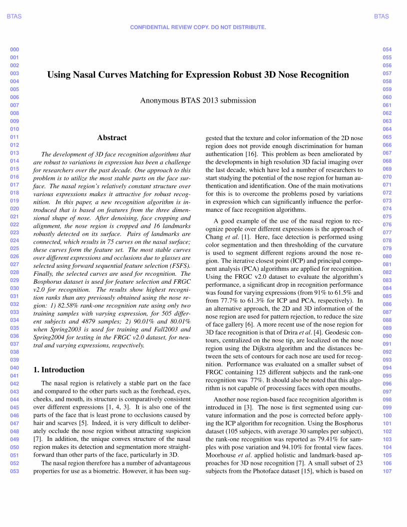
Figure 1: (a) The cropped face region. (b) The binary mapfound by the cylinders intersection with the face surface. (c)The convex hull result. (d) The cropped nose region.

is again cropped and PCA is applied on the newly croppedimage. This simple process helps to localise the tip moreaccurately. After the alignment procedure is completed asmall constant angular rotation along the pitch direction isadded to the face pose as this helps the landmarking algo-rithm to detect the nose root (radix).

The nose region is cropped by finding the intersectionsof three cylinders, each centered on the nose tip, with theface region. Two horizontal cylinders, with radii 40 mm and70 mm, crop the lower and upper parts of the nose, respec-tively. Then, a vertical cylinder, of radius 50 mm, boundsthe nose region on the left and right sides. Applying theseconditions over the X, Y and Z maps results in a binary im-age [Fig. 1(b)], which is further trimmed by morphologicalfilling and convex hull calculation [Fig. 1(c)]. The final bi-nary image is used to find the cropped nose point clouds,see Fig. 1(d). This approach to nose region cropping resultsin fewer redundant regions than the approach of [5] and ismuch faster than that of [4] which uses level set based con-tours.

3. Nasal region landmarking and curves find-ing

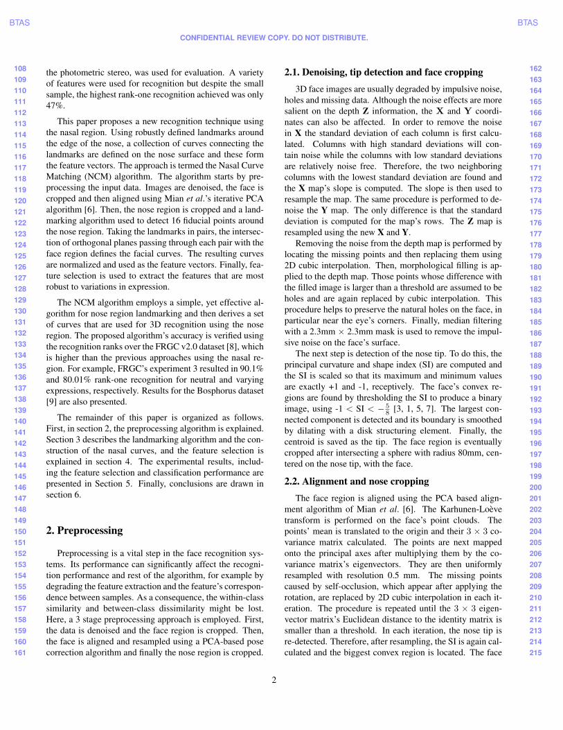
Sixteen landmarks are detected on the nose region, asshown in Fig. 2. A cascade algorithm is used to directlyfind the nose tip (L9), root (L1), and the left (L5) and right(L13) extremities. First, L9 is detected and then used todetect L1, L5 and L13. To avoid selecting incorrect pointsresulting from residual noise or the nostrils as landmarks an

Figure 2: Landmarks’ locations and names.

outlier removal procedure is employed and this procedure isexplained in Section 3.4. The remainder of the landmarksare found by sub-dividing lines connecting the landmarksalready found. In the following subsections the landmark-ing approach is explained in detail.

3.1. Nose tip L9 detection

Although the nose tip has already been approximatelylocalised, it is more accurately fixed in this step. The SI isagain thresholded to extract the largest convex regions fromthe cropped nose region. Then, the nose region’s depth map,Zn, is inverted and the largest connected region is located[5]. The resulting binary image is multiplied by the convexregion to refine it and remove noisy regions. The result is di-lated with a disk structuring element and multiplied by Zn.After median filtering the result, the maximum point is con-sidered as the nose tip. The reason for not directly selectingthe maximum point of Zn as the tip is its vulnerability toresidual spike noise.

3.2. L1 detection

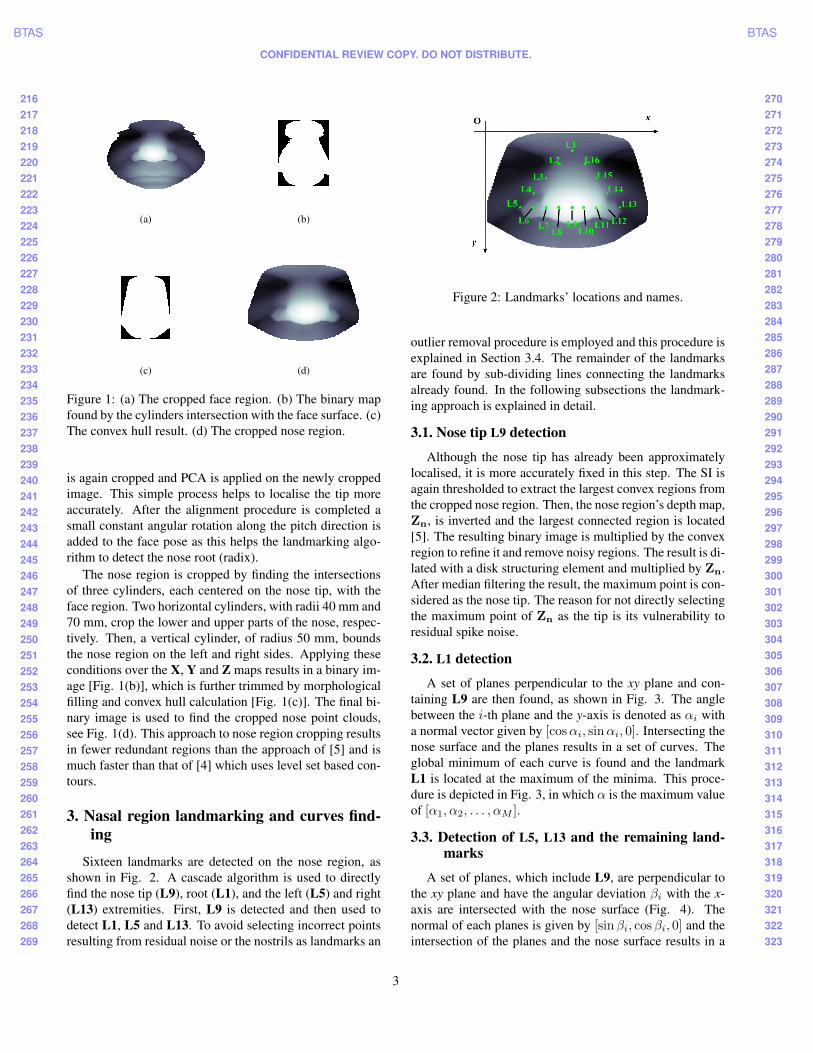
A set of planes perpendicular to the xy plane and con-taining L9 are then found, as shown in Fig. 3. The anglebetween the i-th plane and the y-axis is denoted as αi witha normal vector given by [cosαi, sinαi, 0]. Intersecting thenose surface and the planes results in a set of curves. Theglobal minimum of each curve is found and the landmarkL1 is located at the maximum of the minima. This proce-dure is depicted in Fig. 3, in which α is the maximum valueof [α1, α2, . . . , αM ].

3.3. Detection of L5, L13 and the remaining land-marks

A set of planes, which include L9, are perpendicular tothe xy plane and have the angular deviation βi with the x-axis are intersected with the nose surface (Fig. 4). Thenormal of each planes is given by [sinβi, cosβi, 0] and theintersection of the planes and the nose surface results in a

3

324325326327328329330331332333334335336337338339340341342343344345346347348349350351352353354355356357358359360361362363364365366367368369370371372373374375376377

378379380381382383384385386387388389390391392393394395396397398399400401402403404405406407408409410411412413414415416417418419420421422423424425426427428429430431

BTAS BTAS

CONFIDENTIAL REVIEW COPY. DO NOT DISTRIBUTE.

Figure 3: L1 detection procedure: the blue lines are theplanes intersection. The green curve is each intersection’sminimum. The red dot is the minima peak, which gives thelocation of L1 (α = 15◦).

set of curves (i = 1, . . . , N ). L5 and L13 are located at thepeak position of the curves’ gradient. To do this, each curveis differentiated and the location of the peak values is stored.This results in a set of points on the sides of nasal alar fromwhich the point with the minimum vertical distance fromthe nose tip (L9) are chosen as L5 and L13.

After the four key landmarks were detected, they are pro-jected on the xy plane. The lines connecting the projectionof L1 to L5, L5 to L9, L9 to L13 and L13 to L1 are dividedinto four equal segments and the x and y positions of the re-sulting points are found. The corresponding points on thenose surface give the remaining landmark locations.

3.4. Removal of outlying landmark candidates

As the candidate positions for the landmarks L5 and L13are the positions of maximum gradient on the nose surface,they are sensitive to noise and the position of the nostrils. Inorder to remove incorrect candidate positions an outlier re-moval algorithm is proposed. With reference to Fig. 4, thegradient maxima of the intersection of the planes with thenose surface are marked as green points. However, someoutliers are detected as candidates for L5, in this case dueto the impulsive depth change around the nose tip (locatedwithin the black circle in Fig. 4). To remove the outliersthe distances from the candidate points to the nose tip areclustered using K-means with K = 2. The smallest clusterwill contain the outliers and these points are then replacedby peaks in the surface gradient that are closer to the cen-troid of the larger cluster. The replacement candidates areplotted in red in Fig. 4.

A similar gradient-based approach for detecting the sidenasal landmarks was proposed in [10], where the locationsof the peaks of the gradient on the intersection of a hori-zontal plane passing through the tip and the nose surfacewere selected as L5 and L13. However, by using a set of

Figure 4: L5 (and similarly L13) detection procedure:The blue lines: intersection of the orthogonal planes; Thegreen points: candidate points for L5; The red points:the outlier removal result. β = 15◦ is the maximum of[β1, β2, . . . , βN ]

candidates instead of just a pair and the outlier removal, theapproach proposed above is more robust.

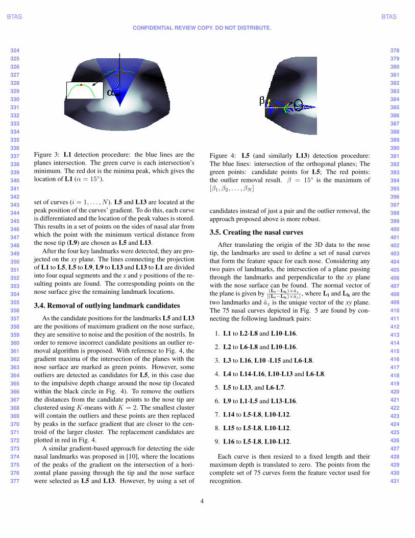
3.5. Creating the nasal curves

After translating the origin of the 3D data to the nosetip, the landmarks are used to define a set of nasal curvesthat form the feature space for each nose. Considering anytwo pairs of landmarks, the intersection of a plane passingthrough the landmarks and perpendicular to the xy planewith the nose surface can be found. The normal vector ofthe plane is given by (Li−Lk)×az

|(Li−Lk)×az| , where Li and Lk are thetwo landmarks and az is the unique vector of the xy plane.The 75 nasal curves depicted in Fig. 5 are found by con-necting the following landmark pairs:

1. L1 to L2-L8 and L10-L16.

2. L2 to L6-L8 and L10-L16.

3. L3 to L16, L10 -L15 and L6-L8.

4. L4 to L14-L16, L10-L13 and L6-L8.

5. L5 to L13, and L6-L7.

6. L9 to L1-L5 and L13-L16.

7. L14 to L5-L8, L10-L12.

8. L15 to L5-L8, L10-L12.

9. L16 to L5-L8, L10-L12.

Each curve is then resized to a fixed length and theirmaximum depth is translated to zero. The points from thecomplete set of 75 curves form the feature vector used forrecognition.

4

432433434435436437438439440441442443444445446447448449450451452453454455456457458459460461462463464465466467468469470471472473474475476477478479480481482483484485

486487488489490491492493494495496497498499500501502503504505506507508509510511512513514515516517518519520521522523524525526527528529530531532533534535536537538539

BTAS BTAS

CONFIDENTIAL REVIEW COPY. DO NOT DISTRIBUTE.

(a) (b)

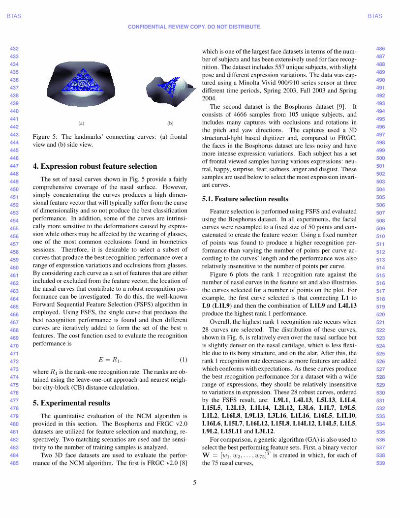
Figure 5: The landmarks’ connecting curves: (a) frontalview and (b) side view.

4. Expression robust feature selectionThe set of nasal curves shown in Fig. 5 provide a fairly

comprehensive coverage of the nasal surface. However,simply concatenating the curves produces a high dimen-sional feature vector that will typically suffer from the curseof dimensionality and so not produce the best classificationperformance. In addition, some of the curves are intrinsi-cally more sensitive to the deformations caused by expres-sion while others may be affected by the wearing of glasses,one of the most common occlusions found in biometricssessions. Therefore, it is desirable to select a subset ofcurves that produce the best recognition performance over arange of expression variations and occlusions from glasses.By considering each curve as a set of features that are eitherincluded or excluded from the feature vector, the location ofthe nasal curves that contribute to a robust recognition per-formance can be investigated. To do this, the well-knownForward Sequential Feature Selection (FSFS) algorithm inemployed. Using FSFS, the single curve that produces thebest recognition performance is found and then differentcurves are iteratively added to form the set of the best nfeatures. The cost function used to evaluate the recognitionperformance is

E = R1. (1)

whereR1 is the rank-one recognition rate. The ranks are ob-tained using the leave-one-out approach and nearest neigh-bor city-block (CB) distance calculation.

5. Experimental resultsThe quantitative evaluation of the NCM algorithm is

provided in this section. The Bosphorus and FRGC v2.0datasets are utilized for feature selection and matching, re-spectively. Two matching scenarios are used and the sensi-tivity to the number of training samples is analyzed.

Two 3D face datasets are used to evaluate the perfor-mance of the NCM algorithm. The first is FRGC v2.0 [8]

which is one of the largest face datasets in terms of the num-ber of subjects and has been extensively used for face recog-nition. The dataset includes 557 unique subjects, with slightpose and different expression variations. The data was cap-tured using a Minolta Vivid 900/910 series sensor at threedifferent time periods, Spring 2003, Fall 2003 and Spring2004.

The second dataset is the Bosphorus dataset [9]. Itconsists of 4666 samples from 105 unique subjects, andincludes many captures with occlusions and rotations inthe pitch and yaw directions. The captures used a 3Dstructured-light based digitizer and, compared to FRGC,the faces in the Bosphorus dataset are less noisy and havemore intense expression variations. Each subject has a setof frontal viewed samples having various expressions: neu-tral, happy, surprise, fear, sadness, anger and disgust. Thesesamples are used below to select the most expression invari-ant curves.

5.1. Feature selection results

Feature selection is performed using FSFS and evaluatedusing the Bosphorus dataset. In all experiments, the facialcurves were resampled to a fixed size of 50 points and con-catenated to create the feature vector. Using a fixed numberof points was found to produce a higher recognition per-formance than varying the number of points per curve ac-cording to the curves’ length and the performance was alsorelatively insensitive to the number of points per curve.

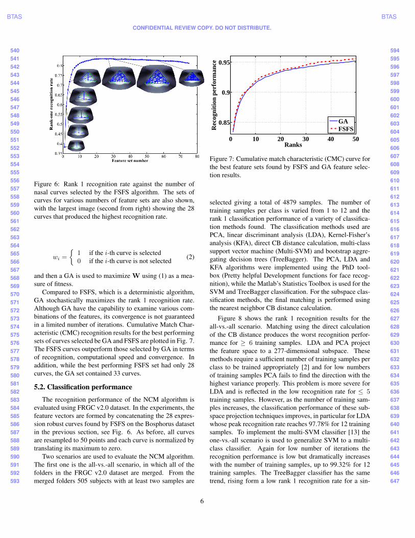
Figure 6 plots the rank 1 recognition rate against thenumber of nasal curves in the feature set and also illustratesthe curves selected for a number of points on the plot. Forexample, the first curve selected is that connecting L1 toL9 (L1L9) and then the combination of L1L9 and L4L13produce the highest rank 1 performance.

Overall, the highest rank 1 recognition rate occurs when28 curves are selected. The distribution of these curves,shown in Fig. 6, is relatively even over the nasal surface butis slightly denser on the nasal cartilage, which is less flexi-ble due to its bony structure, and on the alar. After this, therank 1 recognition rate decreases as more features are addedwhich conforms with expectations. As these curves producethe best recognition performance for a dataset with a widerange of expressions, they should be relatively insensitiveto variations in expression. These 28 robust curves, orderedby the FSFS result, are: L9L1, L4L13, L5L13, L1L4,L15L5, L2L13, L1L14, L2L12, L3L6, L1L7, L9L5,L1L2, L16L8, L9L13, L3L16, L1L16, L16L5, L1L10,L16L6, L15L7, L16L12, L15L8, L14L12, L14L5, L1L5,L9L2, L15L11 and L3L12.

For comparison, a genetic algorithm (GA) is also used toselect the best performing feature sets. First, a binary vectorW = [w1, w2, . . . , w75]

T is created in which, for each ofthe 75 nasal curves,

5

540541542543544545546547548549550551552553554555556557558559560561562563564565566567568569570571572573574575576577578579580581582583584585586587588589590591592593

594595596597598599600601602603604605606607608609610611612613614615616617618619620621622623624625626627628629630631632633634635636637638639640641642643644645646647

BTAS BTAS

CONFIDENTIAL REVIEW COPY. DO NOT DISTRIBUTE.

Figure 6: Rank 1 recognition rate against the number ofnasal curves selected by the FSFS algorithm. The sets ofcurves for various numbers of feature sets are also shown,with the largest image (second from right) showing the 28curves that produced the highest recognition rate.

wi =

{1 if the i-th curve is selected0 if the i-th curve is not selected (2)

and then a GA is used to maximize W using (1) as a mea-sure of fitness.

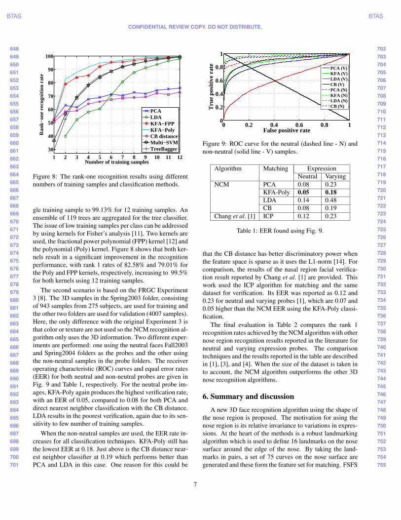
Compared to FSFS, which is a deterministic algorithm,GA stochastically maximizes the rank 1 recognition rate.Although GA have the capability to examine various com-binations of the features, its convergence is not guaranteedin a limited number of iterations. Cumulative Match Char-acteristic (CMC) recognition results for the best performingsets of curves selected be GA and FSFS are plotted in Fig. 7.The FSFS curves outperform those selected by GA in termsof recognition, computational speed and convergence. Inaddition, while the best performing FSFS set had only 28curves, the GA set contained 33 curves.

5.2. Classification performance

The recognition performance of the NCM algorithm isevaluated using FRGC v2.0 dataset. In the experiments, thefeature vectors are formed by concatenating the 28 expres-sion robust curves found by FSFS on the Bosphorus datasetin the previous section, see Fig. 6. As before, all curvesare resampled to 50 points and each curve is normalized bytranslating its maximum to zero.

Two scenarios are used to evaluate the NCM algorithm.The first one is the all-vs.-all scenario, in which all of thefolders in the FRGC v2.0 dataset are merged. From themerged folders 505 subjects with at least two samples are

0 10 20 30 40 50

0.85

0.9

0.95

Ranks

Rec

ogni

tion

per

form

ance

GAFSFS

Figure 7: Cumulative match characteristic (CMC) curve forthe best feature sets found by FSFS and GA feature selec-tion results.

selected giving a total of 4879 samples. The number oftraining samples per class is varied from 1 to 12 and therank 1 classification performance of a variety of classifica-tion methods found. The classification methods used arePCA, linear discriminant analysis (LDA), Kernel-Fisher’sanalysis (KFA), direct CB distance calculation, multi-classsupport vector machine (Multi-SVM) and bootstrap aggre-gating decision trees (TreeBagger). The PCA, LDA andKFA algorithms were implemented using the PhD tool-box (Pretty helpful Development functions for face recog-nition), while the Matlab’s Statistics Toolbox is used for theSVM and TreeBagger classification. For the subspace clas-sification methods, the final matching is performed usingthe nearest neighbor CB distance calculation.

Figure 8 shows the rank 1 recognition results for theall-vs.-all scenario. Matching using the direct calculationof the CB distance produces the worst recognition perfor-mance for ≥ 6 training samples. LDA and PCA projectthe feature space to a 277-dimensional subspace. Thesemethods require a sufficient number of training samples perclass to be trained appropriately [2] and for low numbersof training samples PCA fails to find the direction with thehighest variance properly. This problem is more severe forLDA and is reflected in the low recognition rate for ≤ 5training samples. However, as the number of training sam-ples increases, the classification performance of these sub-space projection techniques improves, in particular for LDAwhose peak recognition rate reaches 97.78% for 12 trainingsamples. To implement the multi-SVM classifier [13] theone-vs.-all scenario is used to generalize SVM to a multi-class classifier. Again for low number of iterations therecognition performance is low but dramatically increaseswith the number of training samples, up to 99.32% for 12training samples. The TreeBagger classifier has the sametrend, rising form a low rank 1 recognition rate for a sin-

6

648649650651652653654655656657658659660661662663664665666667668669670671672673674675676677678679680681682683684685686687688689690691692693694695696697698699700701

702703704705706707708709710711712713714715716717718719720721722723724725726727728729730731732733734735736737738739740741742743744745746747748749750751752753754755

BTAS BTAS

CONFIDENTIAL REVIEW COPY. DO NOT DISTRIBUTE.

1 2 3 4 5 6 7 8 9 10 11 1230

40

50

60

70

80

90

100

Number of training samples

Ran

k−on

e re

cogn

ition

rat

e

PCALDAKFA−FPPKFA−PolyCB distanceMulti−SVMTreeBagger

Figure 8: The rank-one recognition results using differentnumbers of training samples and classification methods.

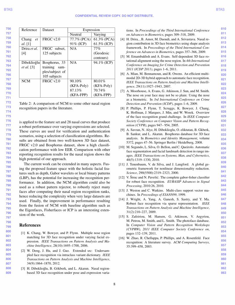
gle training sample to 99.13% for 12 training samples. Anensemble of 119 trees are aggregated for the tree classifier.The issue of low training samples per class can be addressedby using kernels for Fisher’s analysis [11]. Two kernels areused, the fractional power polynomial (FPP) kernel [12] andthe polynomial (Poly) kernel. Figure 8 shows that both ker-nels result in a significant improvement in the recognitionperformance, with rank 1 rates of 82.58% and 79.01% forthe Poly and FPP kernels, respectively, increasing to 99.5%for both kernels using 12 training samples.

The second scenario is based on the FRGC Experiment3 [8]. The 3D samples in the Spring2003 folder, consistingof 943 samples from 275 subjects, are used for training andthe other two folders are used for validation (4007 samples).Here, the only difference with the original Experiment 3 isthat color or texture are not used so the NCM recognition al-gorithm only uses the 3D information. Two different exper-iments are performed: one using the neutral faces Fall2003and Spring2004 folders as the probes and the other usingthe non-neutral samples in the probe folders. The receiveroperating characteristic (ROC) curves and equal error rates(EER) for both neutral and non-neutral probes are given inFig. 9 and Table 1, respectively. For the neutral probe im-ages, KFA-Poly again produces the highest verification rate,with an EER of 0.05, compared to 0.08 for both PCA anddirect nearest neighbor classification with the CB distance.LDA results in the poorest verification, again due to its sen-sitivity to few number of training samples.

When the non-neutral samples are used, the EER rate in-creases for all classification techniques. KFA-Poly still hasthe lowest EER at 0.18. Just above is the CB distance near-est neighbor classifier at 0.19 which performs better thanPCA and LDA in this case. One reason for this could be

0 0.2 0.4 0.6 0.8 10

0.2

0.4

0.6

0.8

1

False positive rate

Tru

e po

siti

ve r

ate

PCA (V)KFA (V)LDA (V)CB (V)PCA (N)KFA (N)LDA (N)CB (N)

Figure 9: ROC curve for the neutral (dashed line - N) andnon-neutral (solid line - V) samples.

Algorithm Matching ExpressionNeutral Varying

NCM PCA 0.08 0.23KFA-Poly 0.05 0.18LDA 0.14 0.48CB 0.08 0.19

Chang et al. [1] ICP 0.12 0.23

Table 1: EER found using Fig. 9.

that the CB distance has better discriminatory power whenthe feature space is sparse as it uses the L1-norm [14]. Forcomparison, the results of the nasal region facial verifica-tion result reported by Chang et al. [1] are provided. Thiswork used the ICP algorithm for matching and the samedataset for verification. Its EER was reported as 0.12 and0.23 for neutral and varying probes [1], which are 0.07 and0.05 higher than the NCM EER using the KFA-Poly classi-fication.

The final evaluation in Table 2 compares the rank 1recognition rates achieved by the NCM algorithm with othernose region recognition results reported in the literature forneutral and varying expression probes. The comparisontechniques and the results reported in the table are describedin [1], [3], and [4]. When the size of the dataset is taken into account, the NCM algorithm outperforms the other 3Dnose recognition algorithms.

6. Summary and discussion

A new 3D face recognition algorithm using the shape ofthe nose region is proposed. The motivation for using thenose region is its relative invariance to variations in expres-sions. At the heart of the methods is a robust landmarkingalgorithm which is used to define 16 landmarks on the nosesurface around the edge of the nose. By taking the land-marks in pairs, a set of 75 curves on the nose surface aregenerated and these form the feature set for matching. FSFS

7

756757758759760761762763764765766767768769770771772773774775776777778779780781782783784785786787788789790791792793794795796797798799800801802803804805806807808809

810811812813814815816817818819820821822823824825826827828829830831832833834835836837838839840841842843844845846847848849850851852853854855856857858859860861862863

BTAS BTAS

CONFIDENTIAL REVIEW COPY. DO NOT DISTRIBUTE.

Reference Dataset ExpressionNeutral Varying

Chang etal. [1]

FRGC v2.0 77.7% (PCA)91% (ICP)

61.3% (PCA)61.5% (ICP)

Drira et al.[4]

FRGC subset,125 subjects

N/A 77%(Geodesiccontours)

Dibekliogluet al. [3]

Bosphorus, 33training sam-ples/subject of105 subjects

N/A 94.1% (ICP)

NCM FRGC v2.0 90.10%(KFA-Poly)87.13%(KFA-FPP)

80.01%(KFA-Poly)70.74%(KFA-FPP)

Table 2: A comparison of NCM to some other nasal regionrecognition papers in the literature.

is applied to the feature set and 28 nasal curves that producea robust performance over varying expressions are selected.These curves are used for verification and authenticationscenarios, using a selection of classification algorithms. Re-sults are obtained from two well-known 3D face dataset,FRGC v2.0 and Bosphorus dataset, show a high classifi-cation performance with low EER. Comparison with otherreporting recognition results for the nasal region shows thehigh potential of our approach.

The current work can be extended in many aspects. Fus-ing the proposed feature space with the holistic facial fea-tures such as depth, Gabor wavelets or local binary patterns(LBP), has the potential for increasing the recognition per-formance. In addition, the NCM algorithm could also beused as a robust pattern rejector, to robustly reject manyfaces after computing their nasal region recognition ranks,hence reducing the complexity when very large datasets areused. Finally, the improvement in performance resultingfrom the fusion of NCM with baseline algorithm such asthe Eigenfaces, Fisherfaces or ICP is an interesting exten-sion of the work.

References[1] K. Chang, W. Bowyer, and P. Flynn. Multiple nose region

matching for 3D face recognition under varying facial ex-pression. IEEE Transactions on Pattern Analysis and Ma-chine Intelligence, 28(10):1695–1700, 2006.

[2] W. Deng, J. Hu, and J. Guo. Extended src: Undersam-pled face recognition via intraclass variant dictionary. IEEETransactions on Pattern Analysis and Machine Intelligence,34(9):1864–1870, 2012.

[3] H. Dibeklioglu, B. Gokberk, and L. Akarun. Nasal region-based 3D face recognition under pose and expression varia-

tions. In Proceedings of the Third International Conferenceon Advances in Biometrics, pages 309–318, 2009.

[4] H. Drira, , B. Amor, M. Daoudi, and A. Srivastava. Nasal re-gion contribution in 3D face biometrics using shape analysisframework. In Proceedings of the Third International Con-ference on Advances in Biometrics, pages 357–366, 2009.

[5] M. Emambakhsh and A. Evans. Self-dependent 3D face ro-tational alignment using the nose region. In 4th InternationalConference on Imaging for Crime Detection and Prevention2011 (ICDP 2011), pages 1–6, 2011.

[6] A. Mian, M. Bennamoun, and R. Owens. An efficient multi-modal 2D-3D hybrid approach to automatic face recognition.IEEE Transactions on Pattern Analysis and Machine Intelli-gence, 29(11):1927–1943, 2007.

[7] A. Moorhouse, A. Evans, G. Atkinson, J. Sun, and M. Smith.The nose on your face may not be so plain: Using the noseas a biometric. In 3rd International Conference on CrimeDetection and Prevention (ICDP), pages 1–6, 2009.

[8] P. Phillips, P. Flynn, T. Scruggs, K. Bowyer, J. Chang,K. Hoffman, J. Marques, J. Min, and W. Worek. Overviewof the face recognition grand challenge. In IEEE ComputerSociety Conference on Computer Vision and Pattern Recog-nition (CVPR), pages 947– 954, 2005.

[9] A. Savran, N. Alyz, H. Dibeklioglu, O. eliktutan, B. Gkberk,B. Sankur, and L. Akarun. Bosphorus database for 3D faceanalysis. In Biometrics and Identity Management, volume5372, pages 47–56. Springer Berlin / Heidelberg, 2008.

[10] M. Segundo, L. Silva, O. Bellon, and C. Queirolo. Automaticface segmentation and facial landmark detection in range im-ages. IEEE Transactions on Systems, Man, and Cybernetics,40(5):1319–1330, 2010.

[11] J. Tenenbaum, V. de Silva, and J. Langford. A global ge-ometric framework for nonlinear dimensionality reduction.Science, 290(5500):2319–2323, 2000.

[12] V. Struc and N. Pavesic. The complete gabor-fisher classifierfor robust face recognition. EURASIP Advances in SignalProcessing, 2010:26, 2010.

[13] J. Weston and C. Watkins. Multi-class support vector ma-chines. In Proceedings of ESANN99, 1999.

[14] J. Wright, A. Yang, A. Ganesh, S. Sastry, and Y. Ma.Robust face recognition via sparse representation. IEEETransactions on Pattern Analysis and Machine Intelligence,31(2):210–227, 2009.

[15] S. Zafeiriou, M. Hansen, G. Atkinson, V. Argyriou,M. Petrou, M. Smith, and L. Smith. The photoface database.In Computer Vision and Pattern Recognition Workshops(CVPRW), 2011 IEEE Computer Society Conference on,pages 132–139, 2011.

[16] W. Zhao, R. Chellappa, P. Phillips, and A. Rosenfeld. Facerecognition: A literature survey. ACM Computing Surveys,35:399–458, 2003.

8