EM Algorithms

Charles Byrne∗and Paul P. B. Eggermont†

September 6, 2012

Abstract

A well studied procedure for estimating a parameter from observed data isto maximize the likelihood function. When a maximizer cannot be obtained inclosed form, iterative maximization algorithms, such as the expectation max-imization (EM) maximum likelihood algorithms, are needed. The standardformulation of the EM algorithms postulates that finding a maximizer of thelikelihood is complicated because the observed data is somehow incompleteor deficient, and the maximization would have been simpler had we observedthe complete data. The EM algorithm involves repeated calculations involvingcomplete data that has been estimated using the current parameter value andconditional expectation. The standard formulation is adequate for the discretecase, in which the random variables involved are governed by finite or infi-nite probability functions, but unsatisfactory in the continuous case, in whichprobability density functions and integrals are needed.

We adopt the view that the observed data is not necessarily incomplete,but just difficult to work with, while different data, which we call the preferreddata, leads to simpler calculations. To relate the preferred data to the observeddata, we assume that the preferred data is acceptable, which means that theconditional distribution of the preferred data, given the observed data, is in-dependent of the parameter. This extension of the EM algorithms containsthe usual formulation for the discrete case, while removing the difficulties as-sociated with the continuous case. Examples are given to illustrate this newapproach.

1 Introduction

We suppose that the observable random vector Y taking values in RN is governed by

a probability density function (pdf) or probability function (pf) of the form fY (y|θ),for some value of the parameter vector θ ∈ Θ, where Θ is the set of all legitimate

∗Charles Byrne@uml.edu, Department of Mathematical Sciences, University of MassachusettsLowell, Lowell, MA 01854, USA

†eggermon@udel.edu, Food and Resource Economics, University of Delaware, Newark, DE 19716,USA

1

values of θ. Our observed data consists of one realization y of Y ; we do not exclude

the possibility that the entries of y are independently obtained samples of a com-

mon real-valued random variable. The true vector of parameters is to be estimated

by maximizing the likelihood function Ly(θ) = fY (y|θ) over all θ ∈ Θ to obtain a

maximum likelihood estimate, θML.

We assume that there is another related random vector X, which we shall call

the preferred data, such that, had we been able to obtain one realization x of X,

maximizing the likelihood function Lx(θ) = fX(x|θ) would have been simpler than

maximizing the likelihood function Ly(θ) = fY (y|θ).The EM algorithm based on X generates a sequence {θk} of parameter vectors.

For the continuous case of probability density functions (pdf), the vector θk+1 is

obtained from θk by maximizing the conditional expected value

E(log fX(X|θ)|y, θk) =

∫fX|Y (x|y, θk) log fX(x|θ)dx; (1.1)

for the discrete case of probability functions (pf), the integral is replaced by a sum-

mation. The EM algorithm is not really a single algorithm, but a framework for

the design of iterative likelihood maximization methods for parameter estimation;

nevertheless, we shall continue to refer to the EM algorithm.

In decreasing order of importance and difficulty, our goals are these:

• 1. to have the sequence of parameters {θk} converging to θML;

• 2. to have the sequence of functions {fX(x|θk)} converging to fX(x|θML);

• 3. to have the sequence of numbers {Ly(θk)} converging to Ly(θML);

• 4. to have the sequence of numbers {Ly(θk)} non-decreasing.

Our focus here will be almost entirely on the fourth goal on the list, with some

discussion of the third goal. We shall discuss the first two goals only for certain

examples.

Our primary objective in this paper is to find a condition on the preferred data

X sufficient to reach the fourth goal. As we shall show, in order to have Ly(θk+1) ≥

Ly(θk), it is sufficient thatX satisfy the acceptability condition fY |X(y|x, θ) = fY |X(y|x).

Our treatment of the EM algorithm differs somewhat from most conventional

presentations, such as those in the fundamental paper [9] and the survey text [19].

As we discuss in more detail in the next section, these conventional treatments are

both restrictive and, in some aspects, incorrect, particularly as they apply to the

2

continuous case. We view our notion of acceptability as a method for correcting these

conventional formulations of the EM algorithm.

We begin by reviewing the conventional formulation of the EM algorithm, pointing

out aspects of that formulation that require correction. We then develop the theory of

the EM for acceptable X, including the involvement of the Kullback-Leibler distance

and the alternating-minimization approach of Csiszar and Tusnady [8]. We then

apply the theory to solve the problem of estimating the mixing proportions in finite

mixtures. The theory in this paper permits us to conclude only that likelihood is

non-decreasing, but by invoking a convergence theorem presented in [5], we are able

to go further and prove convergence of the sequence {θk} to a likelihood maximizer.

2 The Conventional Formulation of EM

By the conventional formulation we mean that given in [9], repeated in [19], and used

in most papers on the subject subsequent to 1977, such as [29] and [20].

2.1 Incomplete and Complete Data

In [9] the fundamental distinction is between incomplete data, our observable Y , and

complete data, our preferred X. The assumption made in [9] is that there is a many-

to-one function h such that Y = h(X); since we can get y from x but not the other

way around, the y is incomplete, while the x is complete.

2.2 Missing Data

It is noted in [9] that their complete-incomplete formulation includes the case of

missing data, and several of the examples they give are of this type. The term

“missing data” is vague, however; any data that we have not observed can be said

to be missing. A close reading of [9] shows that the real problem that can arise

when data is missing, either by failure to report, censoring, or truncation, is that

it complicates the calculations, as with certain types of designed experiments. The

desire to restore the missing data is therefore a desire to simplify the calculations.

The popular example of multinomial data given below illustrates well the point

that one can often choose to view the observed data as “incomplete” simply in order

to introduce “complete” data that makes the calculations simpler, even when there is

no suggestion, in the original problem, that the observed data is in any way inadequate

or “incomplete” . It is in order to emphasize this desire for simplification that we refer

to X as the preferred data, not the complete data.

3

We shall address later the special case we call the missing-data model, in which the

preferred data X takes the form X = Z = (Y,W ), where W is called the missing data

and Z the complete data. Clearly, we have Y = h(X) now, where h is the projection

onto the first coordinate. In this case only do we refer to X as complete. When the

EM algorithm is applied to the missing-data model, the likelihood is non-decreasing,

which suggests that, for an arbitrary preferred data X, we could imagine X as W ,

the missing data, and imagine applying the EM algorithm to Z = (Y,X). This

approach would produce an EM sequence of parameter vectors for which likelihood

is non-decreasing, but it need not be the same sequence as obtained by applying the

EM algorithm to X directly. It is the same sequence, provided that X is acceptable.

We are not suggesting that applying the EM algorithm to Z = (Y,X) would simplify

calculations.

2.3 The Conventional Formulation

The conventional formulation of the problem is that there is a random vector X,

called the “complete data” , taking values in RM , where typically M ≥ N , and often

M > N , with pdf or pf of the form fX(x|θ), and a function h : RM → RN such that

Y = h(X). For example, let X1 and X2 be independent and uniformly distributed on

[0, θ0], X = (X1, X2) and Y = X1 +X2 = h(X). We can use the missing-data model

here with Z = (X1 +X2, X1 −X2). What is missing is not unique, however; instead

of W = X1 −X2 as the missing data, we can use W = X2, or any number of other

combinations of X1 and X2 that would allow us to recapture X.

As we shall attempt to convince the reader, this formulation is somewhat restric-

tive; the main point is simply that fX(x|θ) would have been easier to maximize than

fY (y|θ) is, regardless of the relationship between X and Y . For this reason we shall

call Y the observed data and X the preferred data, and not assume that Y = h(X) for

some function h. We reserve the term complete data for Z of the form Z = (Y,W );

note that, in this case we do have Y = h(Z).

In some applications, the preferred data X arises naturally from the problem,

while in other cases the user must imagine preferred data. This choice in selecting

the preferred data can be helpful in speeding up the algorithm (see [13]).

2.4 A Multinomial Example

In many applications, the entries of the vector y are independent realizations of a

single real-valued or vector-valued random variable V , as they are, at least initially, for

4

finite mixture problems to be considered later. This is not always the case, however,

as the following example shows.

A well known example that was used in [9] and again in [19] to illustrate the

EM algorithm concerns a multinomial model taken from genetics. Here there are

four cells, with cell probabilities 12

+ 14θ0,

14(1 − θ0),

14(1 − θ0), and 1

4θ0, for some

θ0 ∈ Θ = [0, 1] to be estimated. The entries of y are the frequencies from a sample

size of 197. We then have

fY (y|θ) =197!

y1!y2!y3!y4!(1

2+

1

4θ)y1(

1

4(1− θ))y2(

1

4(1− θ))y3(

1

4θ)y4 . (2.1)

It is then supposed that the first of the original four cells can be split into two sub-

cells, with probabilities 12

and 14θ0. We then write y1 = y11 + y12, and let

X = (Y11, Y12, Y2, Y3, Y4), (2.2)

where X has a multinomial distribution with five cells. Note that we do now have

Y = h(X).

This example is a popular one in the literature on the EM algorithm (see [9]

for citations). It is never suggested that the splitting of the first group into two

subgroups is motivated by the demands of the genetics theory itself. As stated in

[19], the motivation for the splitting is to allow us to view the two random variables

Y12 + Y4 and Y2 + Y3 as governed by a binomial distribution; that is, we can view the

value of y12 + y4 as the number of heads, and the value y2 + y3 as the number of tails

that occur in the flipping of a biased coin y12 + y4 + y2 + y3 times. This simplifies the

calculation of the likelihood maximizer.

2.5 Difficulties with the Conventional Formulation

In the literature on the EM algorithm, it is common to assume that there is a function

h : RM → RN such that Y = h(X). In the discrete case, in which summation and

finite or infinite probability functions are involved, we then have

fY (y|θ) =∑

x∈X (y)

fX(x|θ), (2.3)

where

X (y) = {x|h(x) = y} = h−1({y}). (2.4)

The difficulty arises in the continuous case, where integration and probability density

functions (pdf) are needed; the set X (y) can have measure zero in RM , so it is incorrect

5

to mimic Equation (2.3) and write

fY (y|θ) =

∫x∈X (y)

fX(x|θ)dx. (2.5)

The case ofX1 andX2 independent and uniformly distributed on [0, θ0], X = (X1, X2)

and Y = X1 +X2 = h(X) provides a good illustration of the problem. Here X (y) is

the set of all pairs (x1, x2) with y = x1 + x2; this subset of R2 has Lebesgue measure

zero in R2. Now fY |X(y|x, θ) is a delta function, which we may view as δ(x2−(y−x1)),

with the property that∫g(x2)δ(x2 − (y − x1))dx2 = g(y − x1). (2.6)

Then we can write

fY (y|θ) =

∫ ∫δ(x2 − y − x1)fX(x1, x2|θ)dx2dx1 =

∫fX(x1, y − x1)dx1. (2.7)

2.6 A Different Formulation

For any preferred data X the EM algorithm involves two steps: given y and the

current estimate θk, the E-step of the EM algorithm is to calculate

E(log fX(X|θ)|y, θk) =

∫fX|Y (x|y, θk) log fX(x|θ)dx, (2.8)

the conditional expected value of the random vector log fX(X|θ), given y and θk.

Then the M-step is to maximize∫fX|Y (x|y, θk) log fX(x|θ)dx (2.9)

with respect to θ ∈ Θ to obtain θk+1. For the missing-data model Z = (Y,W ), the

M-step is to maximize∫fW |Y (w|y, θk) log fY,W (y, w|θ)dw. (2.10)

We shall also show that for the missing-data model we always have Ly(θk+1) ≥ Ly(θ

k).

For those cases involving continuous distributions in which Y = h(X) the X is

acceptable, but we must define fY |X(y|x) in terms of a delta function; we shall not

consider such cases here.

6

2.7 The Example of Finite Mixtures

We say that a random vector V taking values in RD is a finite mixture if, for j =

1, ..., J , fj is a probability density function or probability function, θj ≥ 0 is a weight,

the θj sum to one, and the probability density function or probability function for V

is

fV (v|θ) =J∑

j=1

θjfj(v). (2.11)

The value of D is unimportant and for simplicity, we shall assume that D = 1.

We draw N independent samples of V , denoted vn, and let yn, the nth entry of

the vector y, be the number vn. To create the preferred data we assume that, for each

n, the number vn is a sample of the random variable Vn whose pdf or pf is fjn , where

the probability that jn = j is θj. We then let the N entries of the preferred data X

be the indices jn. The conditional distribution of Y , given X, is clearly independent

of the parameter vector θ, and is given by

fY (y|x, θ) =N∏

n=1

fjn(yn);

therefore, X is acceptable. Note that we cannot recapture the entries of y from those

of x, so the model Y = h(X) does not hold here. Note also that, although the vector

y is taken originally to be a vector whose entries are independently drawn samples

from V , when we create the preferred data X we change our view of y. Now each

entry of y is governed by a different distribution, so y is no longer viewed as a vector

of independent sample values of a single random vector.

3 The Missing-Data Model

For the missing-data model, the E-step of the EM algorithm is to calculate

E(log fZ(Z|θ)|y, θk) =

∫fW |Y (w|y, θk) log fY,W (y, w|θ)dw. (3.1)

Then the M-step is to maximize∫fW |Y (w|y, θk) log fY,W (y, w|θ)dw (3.2)

to get θk+1. For the missing-data model we have the following result (see [14, 6]).

Proposition 3.1 The sequence {Ly(θk)} is non-decreasing, as k → +∞.

7

Proof: Begin with

log fY (y|θ) =

∫fW |Y (w|y, θk) log fY (y|θ)dw.

Then

log fY (y|θ) =

∫fW |Y (w|y, θk)

(log fY,W (y, w|θ)− log fW |Y (w|y, θ)

)dw.

Therefore,

log fY (y|θk+1)− log fY (y|θk) =∫fW |Y (w|y, θk) log fY,W (y, w|θk+1)dw −

∫fW |Y (w|y, θk) log fY,W (y, w|θk)dw

+

∫fW |Y (w|y, θk) log fW |Y (w|y, θk)dw −

∫fW |Y (w|y, θk) log fW |Y (w|y, θk+1)dw.(3.3)

The first difference on the right side of Equation (3.3) is non-negative because of the

M-step, while the second difference is non-negative because of Jensen’s Inequality.

The fact that likelihood is not decreasing in the missing-data model suggests that

we might try to use this model for arbitrary preferred dataX, by defining the complete

data to be Z = (Y,X) and viewing X as the missing data, that is, W = X. This

approach works, provided that X satisfies the acceptability condition.

4 The EM Algorithm for Acceptable X

For any preferred data X the E-step of the EM algorithm is to calculate

E(log fX(X|θ)|y, θk) =

∫fX|Y (x|y, θk) log fX(x|θ)dx. (4.1)

Once we have y, the M-step is then to maximize

E(log fX(X|θ)|y, θk) =

∫fX|Y (x|y, θk) log fX(x|θ)dx (4.2)

to get θ = θk+1.

4.1 The Likelihood is Non-Decreasing

For the moment, let X be any preferred data. We examine the behavior of the

likelihood when the EM algorithm is applied to X.

8

As in the proof for the missing-data model, we begin with

log fY (y|θ) =

∫fX|Y (x|y, θk) log fY (y|θ)dx.

Then

log fY (y|θ) =

∫fX|Y (x|y, θk)

(log fY,X(y, x|θ)− log fX|Y (x|y, θ)

)dx.

Therefore,

log fY (y|θk+1)− log fY (y|θk) =∫fX|Y (x|y, θk) log fY,X(y, x|θk+1)dx−

∫fX|Y (x|y, θk) log fY,X(y, x|θk)dx

+

∫fX|Y (x|y, θk) log fX|Y (x|y, θk)dx−

∫fX|Y (x|y, θk) log fX|Y (x|y, θk+1)dx. (4.3)

The second difference on the right side of Equation (4.3) is non-negative because of

Jensen’s Inequality. But we cannot assert that the first difference on the right is

non-negative because, in the M-step, we maximize∫fX|Y (x|y, θk) log fX(x|θ)dx

not ∫fX|Y (x|y, θk) log fY,X(y, x|θ)dx.

If X is acceptable, then

log fY,X(y, x|θ)− log fX(x|θ) = log fY |X(y|x) (4.4)

is independent of θ and the difficulty disappears. We may then conclude that likeli-

hood is non-decreasing for acceptable X.

4.2 Generalized EM Algorithms

If, instead of maximizing ∫fX|Y (x|y, θk) log fX(x|θ)dx,

at each M-step, we simply select θk+1 so that∫fX|Y (x|y, θk) log fY,X(y, x|θk+1)dx−

∫fX|Y (x|y, θk) log fY,X(y, x|θk)dx > 0,

we say that we are using a generalized EM (GEM) algorithm. It is clear from the

discussion in the previous subsection that, whenever X is acceptable, a GEM also

guarantees that likelihood is non-decreasing.

9

4.3 Preferred Data as Missing Data

We know that, when the missing-data model is used and the M-step is defined as

maximizing the function in (3.2), the likelihood is not decreasing. It would seem then

that, for any choice of preferred data X, we could view this data as missing and take

as our complete data the pair Z = (Y,X), with X now playing the role of W . The

function in (3.2) is then∫fX|Y (x|y, θk) log fY,X(y, x|θ)dx; (4.5)

we maximize this function to get θk+1. It then follows that Ly(θk+1) ≥ Ly(θ

k). The

obvious question is whether or not these two functions given in (4.1) and (4.5) have

the same maximizers.

For acceptable X we have

log fY,X(y, x|θ) = log fX(x|θ) + log fY |X(y|x), (4.6)

so the two functions given in (4.1) and (4.5) do have the same maximizers. It follows

once again that, whenever the preferred data is acceptable, we have Ly(θk+1) ≥

Ly(θk). Without additional assumptions, however, we cannot conclude that {θk}

converges to θML, nor that {fY (y|θk)} converges to fY (y|θML).

In the discrete case in which Y = h(X) the conditional probability fY |X(y|x, θ) is

δ(y − h(x)), as a function of y, for given x, and is the characteristic function of the

set X (y), as a function of x, for given y. Therefore, we can write

fX|Y (x|y, θ) =

{fX(x|θ)/fY (y|θ), if x ∈ X (y);

0, if x /∈ X (y).(4.7)

For the continuous case in which Y = h(X), the pdf fY |X(y|x, θ) is again a delta

function of y, for given x; the difficulty arises when we need to view this as a function

of x, for given y. The acceptability property helps us avoid this difficulty.

When X is acceptable, we have

fX|Y (x|y, θ) = fY |X(y|x)fX(x|θ)/fY (y|θ), (4.8)

whenever fY (y|θ) 6= 0, and is zero otherwise. Consequently, when X is acceptable,

we have a kernel model for fY (y|θ) in terms of the fX(x|θ):

fY (y|θ) =

∫fY |X(y|x)fX(x|θ)dx; (4.9)

10

for the continuous case we view this as a corrected version of Equation (2.5). In the

discrete case the integral is replaced by a summation, of course, but when we are

speaking generally about either case, we shall use the integral sign.

The acceptability of the missing data W is used in [6], but more for computational

convenience and to involve the Kullback-Leibler distance in the formulation of the

EM algorithm. It is not necessary that W be acceptable in order for likelihood to be

non-decreasing, as we have seen.

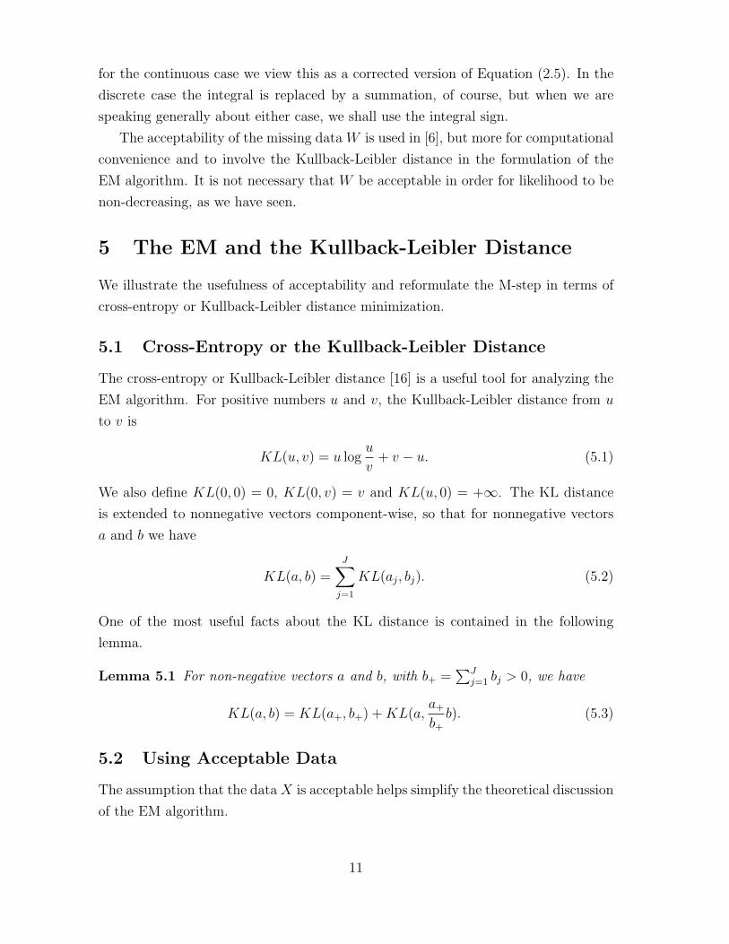
5 The EM and the Kullback-Leibler Distance

We illustrate the usefulness of acceptability and reformulate the M-step in terms of

cross-entropy or Kullback-Leibler distance minimization.

5.1 Cross-Entropy or the Kullback-Leibler Distance

The cross-entropy or Kullback-Leibler distance [16] is a useful tool for analyzing the

EM algorithm. For positive numbers u and v, the Kullback-Leibler distance from u

to v is

KL(u, v) = u logu

v+ v − u. (5.1)

We also define KL(0, 0) = 0, KL(0, v) = v and KL(u, 0) = +∞. The KL distance

is extended to nonnegative vectors component-wise, so that for nonnegative vectors

a and b we have

KL(a, b) =J∑

j=1

KL(aj, bj). (5.2)

One of the most useful facts about the KL distance is contained in the following

lemma.

Lemma 5.1 For non-negative vectors a and b, with b+ =∑J

j=1 bj > 0, we have

KL(a, b) = KL(a+, b+) +KL(a,a+

b+b). (5.3)

5.2 Using Acceptable Data

The assumption that the dataX is acceptable helps simplify the theoretical discussion

of the EM algorithm.

11

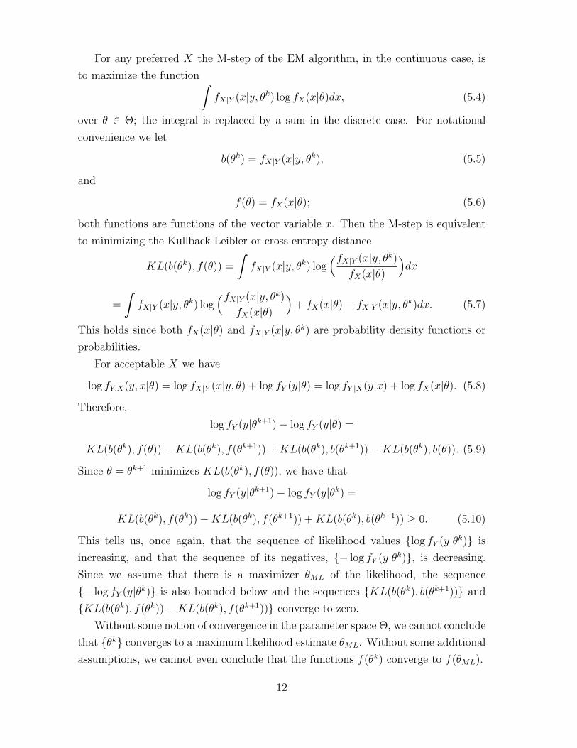
For any preferred X the M-step of the EM algorithm, in the continuous case, is

to maximize the function∫fX|Y (x|y, θk) log fX(x|θ)dx, (5.4)

over θ ∈ Θ; the integral is replaced by a sum in the discrete case. For notational

convenience we let

b(θk) = fX|Y (x|y, θk), (5.5)

and

f(θ) = fX(x|θ); (5.6)

both functions are functions of the vector variable x. Then the M-step is equivalent

to minimizing the Kullback-Leibler or cross-entropy distance

KL(b(θk), f(θ)) =

∫fX|Y (x|y, θk) log

(fX|Y (x|y, θk)

fX(x|θ)

)dx

=

∫fX|Y (x|y, θk) log

(fX|Y (x|y, θk)

fX(x|θ)

)+ fX(x|θ)− fX|Y (x|y, θk)dx. (5.7)

This holds since both fX(x|θ) and fX|Y (x|y, θk) are probability density functions or

probabilities.

For acceptable X we have

log fY,X(y, x|θ) = log fX|Y (x|y, θ) + log fY (y|θ) = log fY |X(y|x) + log fX(x|θ). (5.8)

Therefore,

log fY (y|θk+1)− log fY (y|θ) =

KL(b(θk), f(θ))−KL(b(θk), f(θk+1)) +KL(b(θk), b(θk+1))−KL(b(θk), b(θ)). (5.9)

Since θ = θk+1 minimizes KL(b(θk), f(θ)), we have that

log fY (y|θk+1)− log fY (y|θk) =

KL(b(θk), f(θk))−KL(b(θk), f(θk+1)) +KL(b(θk), b(θk+1)) ≥ 0. (5.10)

This tells us, once again, that the sequence of likelihood values {log fY (y|θk)} is

increasing, and that the sequence of its negatives, {− log fY (y|θk)}, is decreasing.

Since we assume that there is a maximizer θML of the likelihood, the sequence

{− log fY (y|θk)} is also bounded below and the sequences {KL(b(θk), b(θk+1))} and

{KL(b(θk), f(θk))−KL(b(θk), f(θk+1))} converge to zero.

Without some notion of convergence in the parameter space Θ, we cannot conclude

that {θk} converges to a maximum likelihood estimate θML. Without some additional

assumptions, we cannot even conclude that the functions f(θk) converge to f(θML).

12

6 The Approach of Csiszar and Tusnady

For acceptable X the M-step of the EM algorithm is to minimize the function

KL(b(θk), f(θ)) over θ ∈ Θ to get θk+1. To put the EM algorithm into the framework

of the alternating minimization approach of Csiszar and Tusnady [8], we need to view

the M-step in a slightly different way; the problem is that, for the continuous case,

having found θk+1, we do not then minimize KL(b(θ), f(θk+1)) at the next step.

6.1 The Framework of Csiszar and Tusnady

Following [8], we take Ψ(p, q) to be a real-valued function of the variables p ∈ P

and q ∈ Q, where P and Q are arbitrary sets. Minimizing Ψ(p, qn) gives pn+1 and

minimizing Ψ(pn+1, q) gives qn+1, so that

Ψ(pn, qn) ≥ Ψ(pn, qn+1) ≥ Ψ(pn+1, qn+1). (6.1)

The objective is to find (p, q) such that

Ψ(p, q) ≥ Ψ(p, q),

for all p and q. In order to show that {Ψ(pn, qn)} converges to

d = infp∈P,q∈Q

Ψ(p, q)

the authors of [8] assume the three- and four-point properties.

If there is a non-negative function ∆ : P × P → R such that

Ψ(p, qn+1)−Ψ(pn+1, qn+1) ≥ ∆(p, pn+1), (6.2)

then the three-point property holds. If

∆(p, pn) + Ψ(p, q) ≥ Ψ(p, qn+1), (6.3)

for all p and q, then the four-point property holds. Combining these two inequalities,

we have

∆(p, pn)−∆(p, pn+1) ≥ Ψ(pn+1, qn+1)−Ψ(p, q). (6.4)

From the inequality in (6.4) it follows easily that the sequence {Ψ(pn, qn)} converges

to d. Suppose this is not the case. Then there are p′, q′, and D > d with

Ψ(pn, qn) ≥ D > Ψ(p′, q′) ≥ d.

13

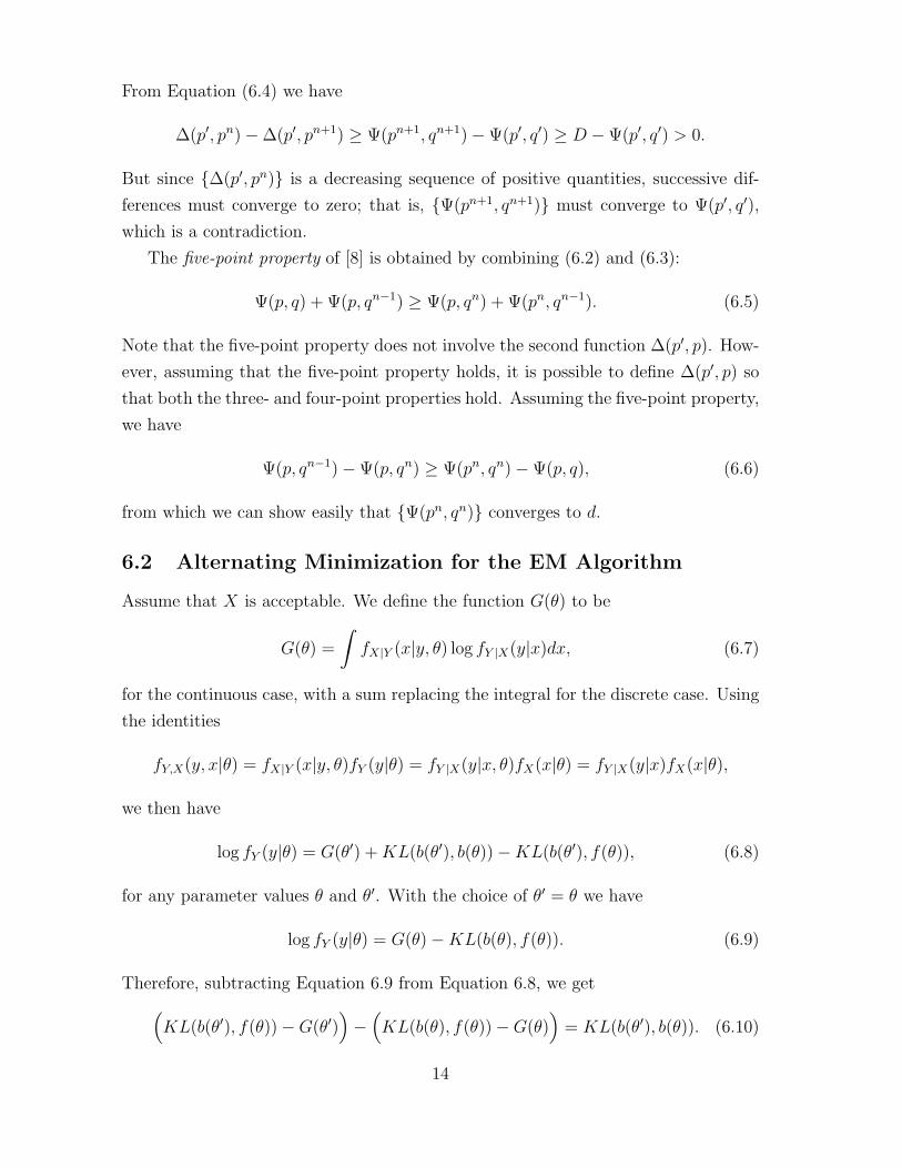
From Equation (6.4) we have

∆(p′, pn)−∆(p′, pn+1) ≥ Ψ(pn+1, qn+1)−Ψ(p′, q′) ≥ D −Ψ(p′, q′) > 0.

But since {∆(p′, pn)} is a decreasing sequence of positive quantities, successive dif-

ferences must converge to zero; that is, {Ψ(pn+1, qn+1)} must converge to Ψ(p′, q′),

which is a contradiction.

The five-point property of [8] is obtained by combining (6.2) and (6.3):

Ψ(p, q) + Ψ(p, qn−1) ≥ Ψ(p, qn) + Ψ(pn, qn−1). (6.5)

Note that the five-point property does not involve the second function ∆(p′, p). How-

ever, assuming that the five-point property holds, it is possible to define ∆(p′, p) so

that both the three- and four-point properties hold. Assuming the five-point property,

we have

Ψ(p, qn−1)−Ψ(p, qn) ≥ Ψ(pn, qn)−Ψ(p, q), (6.6)

from which we can show easily that {Ψ(pn, qn)} converges to d.

6.2 Alternating Minimization for the EM Algorithm

Assume that X is acceptable. We define the function G(θ) to be

G(θ) =

∫fX|Y (x|y, θ) log fY |X(y|x)dx, (6.7)

for the continuous case, with a sum replacing the integral for the discrete case. Using

the identities

fY,X(y, x|θ) = fX|Y (x|y, θ)fY (y|θ) = fY |X(y|x, θ)fX(x|θ) = fY |X(y|x)fX(x|θ),

we then have

log fY (y|θ) = G(θ′) +KL(b(θ′), b(θ))−KL(b(θ′), f(θ)), (6.8)

for any parameter values θ and θ′. With the choice of θ′ = θ we have

log fY (y|θ) = G(θ)−KL(b(θ), f(θ)). (6.9)

Therefore, subtracting Equation 6.9 from Equation 6.8, we get(KL(b(θ′), f(θ))−G(θ′)

)−

(KL(b(θ), f(θ))−G(θ)

)= KL(b(θ′), b(θ)). (6.10)

14

Now we can put the EM algorithm into the alternating-minimization framework.

Define

Ψ(b(θ′), f(θ)) = KL(b(θ′), f(θ))−G(θ′). (6.11)

We know from Equation (6.10) that

Ψ(b(θ′), f(θ))−Ψ(b(θ), f(θ)) = KL(b(θ′), b(θ)). (6.12)

Therefore, we can say that the M-step of the EM algorithm is to minimize Ψ(b(θk), f(θ))

over θ ∈ Θ to get θk+1 and that minimizing Ψ(b(θ), f(θk+1)) gives us θ = θk+1 again.

With the choice of

∆(b(θ′), b(θ)) = KL(b(θ′), b(θ)),

Equation (6.12) becomes

Ψ(b(θ′), f(θ))−Ψ(b(θ), f(θ)) = ∆(b(θ′), b(θ)), (6.13)

which is the three-point property.

With P = B(Θ) and Q = F(Θ) the collections of all functions b(θ) and f(θ), re-

spectively, we can view the EM algorithm as alternating minimization of the function

Ψ(p, q), over p ∈ P and q ∈ Q. As we have seen, the three-point property holds.

What about the four-point property?

The Kullback-Leibler distance is an example of a jointly convex Bregman distance.

According to a lemma of Eggermont and LaRiccia [10, 11], the four-point property

holds for alternating minimization of such distances, using ∆(p′, p) = KL(p′, p), pro-

vided that the objects that can occur in the second-variable position form a convex

subset of RN . In the continuous case of the EM algorithm, we are not performing al-

ternating minimization on the functionKL(b(θ), f(θ′)), but onKL(b(θ), f(θ′))+G(θ).

In the discrete case, whenever Y = h(X), the function G(θ) is always zero, so we are

performing alternating minimization on the KL distance KL(b(θ), f(θ′)). In [2] the

authors consider the problem of minimizing a function of the form

Λ(p, q) = φ(p) + ψ(q) +Dg(p, q), (6.14)

where φ and ψ are convex and differentiable on RJ , Dg is a Bregman distance, and

P = Q is the interior of the domain of g. In [7] it was shown that, when Dg is jointly

convex, the function Λ(p, q) has the five-point property of [8], which is equivalent to

the three- and four-point properties taken together. In some particular instances, the

collection of the functions f(θ) is a convex subset of RJ , as well, so the three- and

four-point properties hold.

15

As we saw previously, to have Ψ(pn, qn) converging to d, it is sufficient that the

five-point property hold. It is conceivable, then, that the five-point property may hold

for Bregman distances under somewhat more general conditions than those employed

in the Eggermont-LaRiccia Lemma.

The five-point property for the EM case is the following:

KL(b(θ), f(θk))−KL(b(θ), f(θk+1)) ≥

(KL(b(θk), f(θk))−G(θk)

)−

(KL(b(θ), f(θ))−G(θ)

). (6.15)

7 Sums of Independent Poisson Random Variables

The EM is often used with aggregated data. The case of sums of independent Poisson

random variables is particularly important.

7.1 Poisson Sums

LetX1, ..., XN be independent Poisson random variables with expected value E(Xn) =

λn. Let X be the random vector with Xn as its entries, λ the vector whose entries

are the λn, and λ+ =∑N

n=1 λn. Then the probability function for X is

fX(x|λ) =N∏

n=1

λxnn exp(−λn)/xn! = exp(−λ+)

N∏n=1

λxnn /xn! . (7.1)

Now let Y =∑N

n=1Xn. Then, the probability function for Y is

Prob(Y = y) = Prob(X1 + ...+XN = y)

=∑

x1+...xN=y

exp(−λ+)N∏

n=1

λxnn /xn! . (7.2)

As we shall see shortly, we have

∑x1+...xN=y

exp(−λ+)N∏

n=1

λxnn /xn! = exp(−λ+)λy

+/y! . (7.3)

Therefore, Y is a Poisson random variable with E(Y ) = λ+.

When we observe an instance of Y , we can consider the conditional distribution

fX|Y (x|y, λ) of {X1, ..., XN}, subject to y = X1 + ...+XN . We have

fX|Y (x|y, λ) =y!

x1!...xN !

( λ1

λ+

)x1

...(λN

λ+

)xN

. (7.4)

16

This is a multinomial distribution.

Given y and λ, the conditional expected value of Xn is then

E(Xn|y, λ) = yλn/λ+.

To see why this is true, consider the marginal conditional distribution fX1|Y (x1|y, λ)

of X1, conditioned on y and λ, which we obtain by holding x1 fixed and summing

over the remaining variables. We have

fX1|Y (x1|y, λ) =y!

x1!(y − x1)!

( λ1

λ+

)x1(λ′+λ+

)y−x1 ∑x2+...+xN=y−x1

(y − x1)!

x2!...xN !

N∏n=2

(λn

λ′+

)xn

,

where

λ′+ = λ+ − λ1.

As we shall show shortly,

∑x2+...+xN=y−x1

(y − x1)!

x2!...xN !

N∏n=2

(λn

λ′+

)xn

= 1,

so that

fX1|Y (x1|y, λ) =y!

x1!(y − x1)!

( λ1

λ+

)x1(λ′+λ+

)y−x1

.

The random variable X1 is equivalent to the random number of heads showing in

y flips of a coin, with the probability of heads given by λ1/λ+. Consequently, the

conditional expected value of X1 is yλ1/λ+, as claimed. In the next subsection we

look more closely at the multinomial distribution.

7.2 The Multinomial Distribution

When we expand the quantity (a1 + ...+aN)y, we obtain a sum of terms, each having

the form ax11 ...a

xNN , with x1 + ... + xN = y. How many terms of the same form are

there? There are N variables an. We are to use xn of the an, for each n = 1, ..., N ,

to get y = x1 + ... + xN factors. Imagine y blank spaces, each to be filled in by a

variable as we do the selection. We select x1 of these blanks and mark them a1. We

can do that in(

yx1

)ways. We then select x2 of the remaining blank spaces and enter

a2 in them; we can do this in(

y−x1

x2

)ways. Continuing in this way, we find that we

can select the N factor types in(y

x1

)(y − x1

x2

)...

(y − (x1 + ...+ xN−2)

xN−1

)(7.5)

17

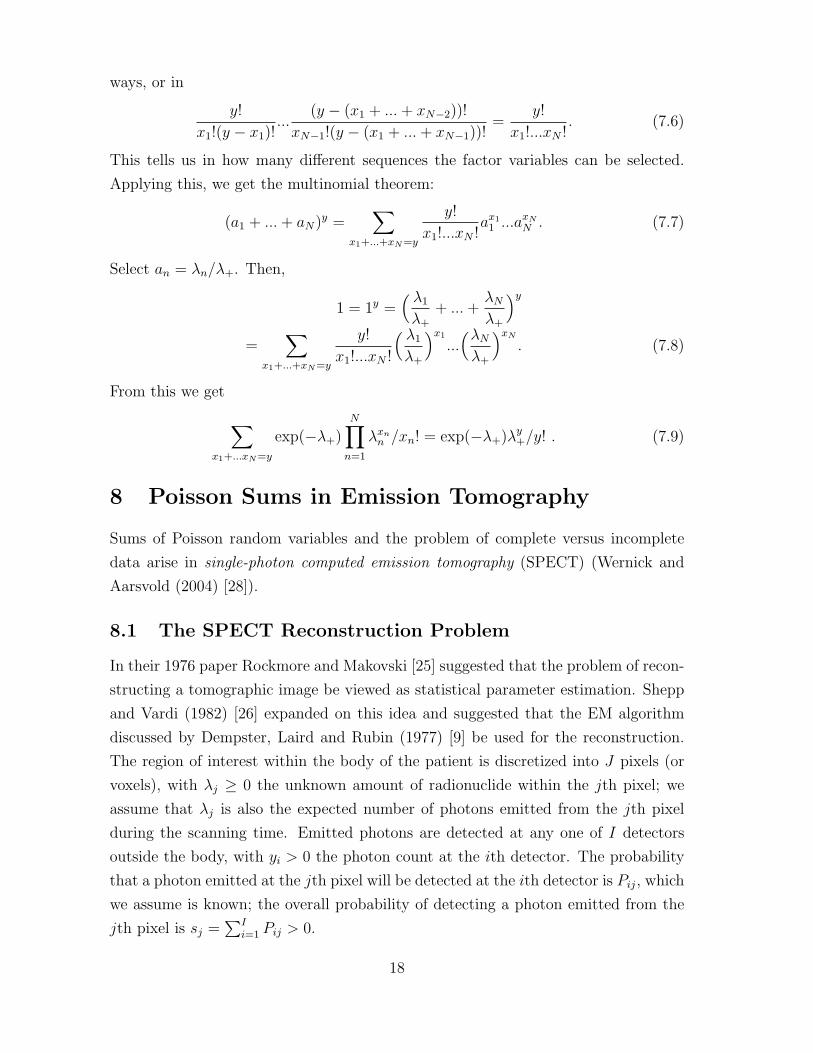
ways, or in

y!

x1!(y − x1)!...

(y − (x1 + ...+ xN−2))!

xN−1!(y − (x1 + ...+ xN−1))!=

y!

x1!...xN !. (7.6)

This tells us in how many different sequences the factor variables can be selected.

Applying this, we get the multinomial theorem:

(a1 + ...+ aN)y =∑

x1+...+xN=y

y!

x1!...xN !ax1

1 ...axNN . (7.7)

Select an = λn/λ+. Then,

1 = 1y =( λ1

λ+

+ ...+λN

λ+

)y

=∑

x1+...+xN=y

y!

x1!...xN !

( λ1

λ+

)x1

...(λN

λ+

)xN

. (7.8)

From this we get

∑x1+...xN=y

exp(−λ+)N∏

n=1

λxnn /xn! = exp(−λ+)λy

+/y! . (7.9)

8 Poisson Sums in Emission Tomography

Sums of Poisson random variables and the problem of complete versus incomplete

data arise in single-photon computed emission tomography (SPECT) (Wernick and

Aarsvold (2004) [28]).

8.1 The SPECT Reconstruction Problem

In their 1976 paper Rockmore and Makovski [25] suggested that the problem of recon-

structing a tomographic image be viewed as statistical parameter estimation. Shepp

and Vardi (1982) [26] expanded on this idea and suggested that the EM algorithm

discussed by Dempster, Laird and Rubin (1977) [9] be used for the reconstruction.

The region of interest within the body of the patient is discretized into J pixels (or

voxels), with λj ≥ 0 the unknown amount of radionuclide within the jth pixel; we

assume that λj is also the expected number of photons emitted from the jth pixel

during the scanning time. Emitted photons are detected at any one of I detectors

outside the body, with yi > 0 the photon count at the ith detector. The probability

that a photon emitted at the jth pixel will be detected at the ith detector is Pij, which

we assume is known; the overall probability of detecting a photon emitted from the

jth pixel is sj =∑I

i=1 Pij > 0.

18

8.1.1 The Preferred Data

For each i and j the random variable Xij is the number of photons emitted from the

jth pixel and detected at the ith detector; the Xij are assumed to be independent

and Pijλj-Poisson. With xij a realization of Xij, the vector x with components xij is

our preferred data. The pdf for this preferred data is a probability vector, with

fX(x|λ) =I∏

i=1

J∏j=1

exp−Pijλj(Pijλj)xij/xij! . (8.1)

Given an estimate λk of the vector λ and the restriction that Yi =∑J

j=1Xij, the

random variables Xi1, ..., XiJ have the multinomial distribution

Prob(xi1, ..., xiJ) =yi!

xi1! · · · xiJ !

J∏j=1

( Pijλj

(Pλ)i

)xij

.

Therefore, the conditional expected value of Xij, given y and λk, is

E(Xij|y, λk) = λkjPij

( yi

(Pλk)i

),

and the conditional expected value of the random variable

log fX(X|λ) =I∑

i=1

J∑j=1

(−Pijλj) +Xij log(Pijλj) + constants

becomes

E(log fX(X|λ)|y, λk) =I∑

i=1

J∑j=1

((−Pijλj) + λk

jPij

( yi

(Pλk)i

)log(Pijλj)

),

omitting terms that do not involve the parameter vector λ. In the EM algorithm, we

obtain the next estimate λk+1 by maximizing E(log fX(X|λ)|y, λk).

The log likelihood function for the preferred data X (omitting constants) is

LLx(λ) =I∑

i=1

J∑j=1

(− Pijλj +Xij log(Pijλj)

). (8.2)

Of course, we do not have the complete data.

8.1.2 The Incomplete Data

What we do have are the yi, values of the random variables

Yi =J∑

j=1

Xij; (8.3)

19

this is the given data. These random variables are also independent and (Pλ)i-

Poisson, where

(Pλ)i =J∑

j=1

Pijλj.

The log likelihood function for the given data is

LLy(λ) =I∑

i=1

(− (Pλ)i + yi log((Pλ)i)

). (8.4)

Maximizing LLx(λ) in Equation (8.2) is easy, while maximizing LLy(λ) in Equation

(8.4) is harder and requires an iterative method.

The EM algorithm involves two steps: in the E-step we compute the conditional

expected value of LLx(λ), conditioned on the data vector y and the current estimate

λk of λ; in the M-step we maximize this conditional expected value to get the next

λk+1. Putting these two steps together, we have the following EMML iteration:

λk+1j = λk

j s−1j

I∑i=1

Pijyi

(Pλk)i

. (8.5)

For any positive starting vector λ0, the sequence {λk} converges to a maximizer of

LLy(λ), over all non-negative vectors λ.

Note that, because we are dealing with finite probability vectors in this example,

it is a simple matter to conclude that

fY (y|λ) =∑

x∈X (y)

fX(x|λ). (8.6)

8.2 Using the KL Distance

In this subsection we assume, for notational convenience, that the system y = Pλ

has been normalized so that sj = 1 for each j. Maximizing E(log fX(X|λ)|y, λk) is

equivalent to minimizing KL(r(λk), q(λ)), where r(λ) and q(λ) are I by J arrays with

entries

r(λ)ij = λjPij

( yi

(Pλ)i

),

and

q(λ)ij = λjPij.

In terms of our previous notation we identify r(λ) with b(θ), and q(λ) with f(θ). The

set F(Θ) of all f(θ) is now a convex set and the four-point property of [8] holds. The

20

iterative step of the EMML algorithm is then

λk+1j = λk

j

I∑i=1

Pi,jyi

(Pλk)i

. (8.7)

The sequence {λk} converges to a maximizer λML of the likelihood for any positive

starting vector.

As we noted previously, before we can discuss the possible convergence of the

sequence {λk} of parameter vectors to a maximizer of the likelihood, it is necessary to

have a notion of convergence in the parameter space. For the problem in this section,

the parameter vectors λ are non-negative. Proof of convergence of the sequence {λk}depends heavily on the following [4]:

KL(y, Pλk)−KL(y, Pλk+1) = KL(r(λk), r(λk+1)) +KL(λk+1, λk); (8.8)

and

KL(λML, λk)−KL(λML, λ

k+1) ≥ KL(y, Pλk)−KL(y, PλML). (8.9)

Any likelihood maximizer λML is also a non-negative minimizer of the KL distance

KL(y, Pλ), so the EMML algorithm can be thought of as a method for finding a non-

negative solution (or approximate solution) for a system y = Pλ of linear equations

in which yi > 0 and Pij ≥ 0 for all indices. This will be helpful when we consider

mixture problems.

9 Finite Mixture Problems

Estimating the combining proportions in probabilistic mixture problems shows that

there are meaningful examples of our acceptable-data model, and provides important

applications of likelihood maximization.

9.1 Mixtures

We say that a random vector V taking values in RD is a finite mixture (see [12, 24])

if there are probability density functions or probabilities fj and numbers θj ≥ 0, for

j = 1, ..., J , such that the probability density function or probability function for V

has the form

fV (v|θ) =J∑

j=1

θjfj(v), (9.1)

for some choice of the θj ≥ 0 with∑J

j=1 θj = 1. As previously, we shall assume,

without loss of generality, that D = 1.

21

9.2 The Likelihood Function

The data are N realizations of the random variable V , denoted vn, for n = 1, ..., N ,

and the given data is the vector y = (v1, ..., vN). The column vector θ = (θ1, ..., θJ)T

is the generic parameter vector of mixture combining proportions. The likelihood

function is

Ly(θ) =N∏

n=1

(θ1f1(vn) + ...+ θJfJ(vn)

). (9.2)

Then the log likelihood function is

LLy(θ) =N∑

n=1

log(θ1f1(vn) + ...+ θJfJ(vn)

).

With u the column vector with entries un = 1/N , and P the matrix with entries

Pnj = fj(vn), we define

sj =N∑

n=1

Pnj =N∑

n=1

fj(vn).

Maximizing LLy(θ) is equivalent to minimizing

F (θ) = KL(u, Pθ) +J∑

j=1

(1− sj)θj. (9.3)

9.3 A Motivating Illustration

To motivate such mixture problems, we imagine that each data value is generated by

first selecting one value of j, with probability θj, and then selecting a realization of a

random variable governed by fj(v). For example, there could be J bowls of colored

marbles, and we randomly select a bowl, and then randomly select a marble within

the selected bowl. For each n the number vn is the numerical code for the color of the

nth marble drawn. In this illustration we are using a mixture of probability functions,

but we could have used probability density functions.

9.4 The Acceptable Data

We approach the mixture problem by creating acceptable data. We imagine that we

could have obtained xn = jn, for n = 1, ..., N , where the selection of vn is governed by

the function fjn(v). In the bowls example, jn is the number of the bowl from which the

nth marble is drawn. The acceptable-data random vector is X = (X1, ..., XN), where

22

the Xn are independent random variables taking values in the set {j = 1, ..., J}. The

value jn is one realization of Xn. Since our objective is to estimate the true θj, the

values vn are now irrelevant. Our ML estimate of the true θj is simply the proportion

of times j = jn. Given a realization x of X, the conditional pdf or pf of Y does not

involve the mixing proportions, so X is acceptable. Notice also that it is not possible

to calculate the entries of y from those of x; the model Y = h(X) does not hold.

9.5 The Mix-EM Algorithm

Using this acceptable data, we derive the EM algorithm, which we call the Mix-EM

algorithm.

With Nj denoting the number of times the value j occurs as an entry of x, the

likelihood function for X is

Lx(θ) = fX(x|θ) =J∏

j=1

θNj

j , (9.4)

and the log likelihood is

LLx(θ) = logLx(θ) =J∑

j=1

Nj log θj. (9.5)

Then

E(logLx(θ)|y, θk) =J∑

j=1

E(Nj|y, θk) log θj. (9.6)

To simplify the calculations in the E-step we rewrite LLx(θ) as

LLx(θ) =N∑

n=1

J∑j=1

Xnj log θj, (9.7)

where Xnj = 1 if j = jn and zero otherwise. Then we have

E(Xnj|y, θk) = prob (Xnj = 1|y, θk) =θk

j fj(vn)

f(vn|θk). (9.8)

The function E(LLx(θ)|y, θk) becomes

E(LLx(θ)|y, θk) =N∑

n=1

J∑j=1

θkj fj(vn)

f(vn|θk)log θj. (9.9)

23

Maximizing with respect to θ, we get the iterative step of the Mix-EM algorithm:

θk+1j =

1

Nθk

j

N∑n=1

fj(vn)

f(vn|θk). (9.10)

We know from our previous discussions that, since the preferred data X is accept-

able, likelihood is non-decreasing for this algorithm. We shall go further now, and

show that the sequence of probability vectors {θk} converges to a maximizer of the

likelihood.

9.6 Convergence of the Mix-EM Algorithm

As we noted earlier, maximizing the likelihood in the mixture case is equivalent to

minimizing

F (θ) = KL(u, Pθ) +J∑

j=1

(1− sj)θj,

over probability vectors θ. It is easily shown that, if θ minimizes F (θ) over all non-

negative vectors θ, then θ is a probability vector. Therefore, we can obtain the

maximum likelihood estimate of θ by minimizing F (θ) over non-negative vectors θ.

The following theorem is found in [5].

Theorem 9.1 Let u be any positive vector, P any non-negative matrix with sj > 0

for each j, and

F (θ) = KL(u, Pθ) +J∑

j=1

βjKL(γj, θj).

If sj + βj > 0, αj = sj/(sj + βj), and βjγj ≥ 0, for all j, then the iterative sequence

given by

θk+1j = αjs

−1j θk

j

( N∑n=1

Pn,jun

(Pθk)n

)+ (1− αj)γj (9.11)

converges to a non-negative minimizer of F (θ).

With the choices un = 1/N , γj = 0, and βj = 1− sj, the iteration in Equation (9.11)

becomes that of the Mix-EM algorithm. Therefore, the sequence {θk} converges to

the maximum likelihood estimate of the mixing proportions.

24

10 More on Convergence

There is a mistake in the proof of convergence given in Dempster, Laird, and Rubin

(1977) [9]. Wu (1983) [29] and Boyles (1983) [3] attempted to repair the error, but also

gave examples in which the EM algorithm failed to converge to a global maximizer

of likelihood. In Chapter 3 of McLachlan and Krishnan (1997) [19] we find the basic

theory of the EM algorithm, including available results on convergence and the rate of

convergence. Because many authors rely on Equation (2.5), it is not clear that these

results are valid in the generality in which they are presented. There appears to be

no single convergence theorem that is relied on universally; each application seems to

require its own proof of convergence. When the use of the EM algorithm was suggested

for SPECT and PET, it was necessary to prove convergence of the resulting iterative

algorithm in Equation (8.5), as was eventually achieved in a sequence of papers (Shepp

and Vardi (1982) [26], Lange and Carson (1984) [17], Vardi, Shepp and Kaufman

(1985) [27], Lange, Bahn and Little (1987) [18], and Byrne (1993) [4]). When the

EM algorithm was applied to list-mode data in SPECT and PET (Barrett, White,

and Parra (1997) [1, 23], and Huesman et al. (2000) [15]), the resulting algorithm

differed slightly from that in Equation (8.5) and a proof of convergence was provided

in Byrne (2001) [5]. The convergence theorem in Byrne (2001) also establishes the

convergence of the iteration in Equation (9.10) to the maximum-likelihood estimate

of the mixing proportions.

11 Open Questions

As we have seen, the conventional formulation of the EM algorithm presents difficul-

ties when probability density functions are involved. We have shown here that the

use of acceptable preferred data can be helpful in resolving this issue, but other ways

may also be useful.

Proving convergence of the sequence {θk} appears to involve the selection of an

appropriate topology for the parameter space Θ. While it is common to assume that

Θ is a subset of Euclidean space and that the usual norm should be used to define

distance, it may be helpful to tailor the metric to the nature of the parameters. In

the case of Poisson sums, for example, the parameters are non-negative vectors and

we found that the cross-entropy distance is more appropriate. Even so, additional

assumptions appear necessary before convergence of the {θk} can be established. To

simplify the analysis, it is often assumed that cluster points of the sequence lie in the

25

interior of the set Θ, which is not a realistic assumption in some applications.

It may be wise to consider, instead, convergence of the functions fX(x|θk), or

maybe even to identify the parameters θ with the functions fX(x|θ). Proving conver-

gence to Ly(θML) of the likelihood values Ly(θk) is also an option.

12 Conclusion

Difficulties with the conventional formulation of the EM algorithm in the continuous

case of probability density functions (pdf) has prompted us to adopt a new definition,

that of acceptable data. As we have shown, this model can be helpful in generating

EM algorithms in a variety of situations. For the discrete case of probability functions

(pf), the conventional approach remains satisfactory. In both cases, the two steps of

the EM algorithm can be viewed as alternating minimization of the Kullback-Leibler

distance between two sets of parameterized pf or pdf, along the lines investigated by

Csiszar and Tusnady [8]. In order to use the full power of their theory, however, we

need one of the sets to be convex. This does occur in the important special case of

sums of independent Poisson random variables, but is not generally the case.

References

1. Barrett, H., White, T., and Parra, L. (1997) “List-mode likelihood.”J. Opt. Soc.

Am. A 14, pp. 2914–2923.

2. Bauschke, H., Combettes, P., and Noll, D. (2006) “Joint minimization with al-

ternating Bregman proximity operators.” Pacific Journal of Optimization, 2, pp.

401–424.

3. Boyles, R. (1983) “On the convergence of the EM algorithm.” Journal of the

Royal Statistical Society B, 45, pp. 47–50.

4. Byrne, C. (1993) “Iterative image reconstruction algorithms based on cross-

entropy minimization.”IEEE Transactions on Image Processing IP-2, pp. 96–103.

5. Byrne, C. (2001) “Likelihood maximization for list-mode emission tomographic

image reconstruction.”IEEE Transactions on Medical Imaging 20(10), pp. 1084–

1092.

6. Byrne, C., and Eggermont, P. (2011) “EM Algorithms.” in Handbook of Mathe-

matical Methods in Imaging, Otmar Scherzer, ed., Springer-Science.

26

7. Byrne, C. (2012) “Alternating and sequential unconstrained minimization algo-

rithms.” Journal of Optimization Theory and Applications, electronic 154(3),

DOI 10.1007/s1090134-2, (2012); hardcopy 156(2), February, 2013.

8. Csiszar, I. and Tusnady, G. (1984) “Information geometry and alternating mini-

mization procedures.”Statistics and Decisions Supp. 1, pp. 205–237.

9. Dempster, A.P., Laird, N.M. and Rubin, D.B. (1977) “Maximum likelihood from

incomplete data via the EM algorithm.”Journal of the Royal Statistical Society,

Series B 37, pp. 1–38.

10. Eggermont, P.P.B., LaRiccia, V.N. (1995) “Smoothed maximum likelihood den-

sity estimation for inverse problems.” Annals of Statistics 23, pp. 199–220.

11. Eggermont, P., and LaRiccia, V. (2001) Maximum Penalized Likelihood Estima-

tion, Volume I: Density Estimation. New York: Springer.

12. Everitt, B. and Hand, D. (1981) Finite Mixture Distributions London: Chapman

and Hall.

13. Fessler, J., Ficaro, E., Clinthorne, N., and Lange, K. (1997) “Grouped-coordinate

ascent algorithms for penalized-likelihood transmission image reconstruction.”

IEEE Transactions on Medical Imaging, 16 (2), pp. 166–175.

14. Hogg, R., McKean, J., and Craig, A. (2004) Introduction to Mathematical Statis-

tics, 6th edition, Prentice Hall.

15. Huesman, R., Klein, G., Moses, W., Qi, J., Ruetter, B., and Virador, P.

(2000) “List-mode maximum likelihood reconstruction applied to positron emis-

sion mammography (PEM) with irregular sampling.”IEEE Transactions on Med-

ical Imaging 19 (5), pp. 532–537.

16. Kullback, S. and Leibler, R. (1951) “On information and sufficiency.”Annals of

Mathematical Statistics 22, pp. 79–86.

17. Lange, K. and Carson, R. (1984) “EM reconstruction algorithms for emission

and transmission tomography.”Journal of Computer Assisted Tomography 8, pp.

306–316.

18. Lange, K., Bahn, M. and Little, R. (1987) “A theoretical study of some maximum

likelihood algorithms for emission and transmission tomography.”IEEE Trans.

Med. Imag. MI-6(2), pp. 106–114.

27

19. McLachlan, G.J. and Krishnan, T. (1997) The EM Algorithm and Extensions.

New York: John Wiley and Sons, Inc.

20. Meng, X., and Pedlow, S. (1992) “EM: a bibliographic review with missing ar-

ticles.” Proceedings of the Statistical Computing Section, American Statistical

Association, American Statistical Association, Alexandria, VA.

21. Meng, X., and van Dyk, D. (1997) “The EM algorithm- An old folk-song sung to

a fast new tune.” J. R. Statist. Soc. B, 59(3), pp. 511–567.

22. Narayanan, M., Byrne, C. and King, M. (2001) “An interior point iterative

maximum-likelihood reconstruction algorithm incorporating upper and lower

bounds with application to SPECT transmission imaging.”IEEE Transactions

on Medical Imaging TMI-20 (4), pp. 342–353.

23. Parra, L. and Barrett, H. (1998) “List-mode likelihood: EM algorithm and image

quality estimation demonstrated on 2-D PET.”IEEE Transactions on Medical

Imaging 17, pp. 228–235.

24. Redner, R., and Walker, H. (1984) “Mixture Densities, Maximum Likelihood and

the EM Algorithm.” SIAM Review, 26(2), pp. 195–239.

25. Rockmore, A., and Macovski, A. (1976) “A maximum likelihood approach to

emission image reconstruction from projections.” IEEE Transactions on Nuclear

Science, NS-23, pp. 1428–1432.

26. Shepp, L., and Vardi, Y. (1982) “Maximum likelihood reconstruction for emission

tomography.” IEEE Transactions on Medical Imaging, MI-1, pp. 113–122.

27. Vardi, Y., Shepp, L.A. and Kaufman, L. (1985) “A statistical model for positron

emission tomography.”Journal of the American Statistical Association 80, pp.

8–20.

28. Wernick, M. and Aarsvold, J., editors (2004) Emission Tomography: The Funda-

mentals of PET and SPECT. San Diego: Elsevier Academic Press.

29. Wu, C.F.J. (1983) “On the convergence properties of the EM algorithm.” Annals

of Statistics, 11, pp. 95–103.

28