ELMOPP: an application of graphtheory and machine learning to

traffic light coordinationFareed Sheriff

Center for Medical Sciences, Mills Godwin High School, Henrico, Virginia, USA

Abstract

Purpose –This paper presents the Edge LoadManagement and Optimization through Pseudoflow Prediction(ELMOPP) algorithm, which aims to solve problems detailed in previous algorithms; throughmachine learningwith nested long short-termmemory (NLSTM)modules and graph theory, the algorithm attempts to predict thenear future using past data and traffic patterns to inform its real-time decisions and better mitigate traffic bypredicting future traffic flow based on past flow and using those predictions to both maximize present trafficflow and decrease future traffic congestion.Design/methodology/approach – ELMOPP was tested against the ITLC and OAF traffic managementalgorithms using a simulation modeled after the one presented in the ITLC paper, a single-intersectionsimulation.Findings – The collected data supports the conclusion that ELMOPP statistically significantlyoutperforms both algorithms in throughput rate, a measure of how many vehicles are able to exit inroadsevery second.Originality/value – Furthermore, while ITLC and OAF require the use of GPS transponders and GPS, speedsensors and radio, respectively, ELMOPP only uses traffic light camera footage, something that is almostalways readily available in contrast to GPS and speed sensors.

Keywords LSTM, Traffic management algorithm, Traffic prediction

Paper type Research paper

1. Introduction1.1 BackgroundTraffic lights used specifically for road systems have been around since the 19th centurywith the installation of a gas-lit traffic light in London. This traffic light was a single lightthat controlled horse-drawn carriage traffic and was prone to explosions. This was soonfollowed by the first electric light, installed in Ohio in 1914; this was also a stand-alonetraffic light. The first network of traffic lights was implemented in Salt Lake City, Utah in1917 as a collection of six traffic lights controlled through a manual switch. The purpose oftraffic lights was to control traffic to prevent jams and decrease the risk of accidents. This isa heavy task to conduct manually because it requires that humans decide the optimal oreven just an adequate configuration of traffic light timings to minimize traffic congestion,which becomes increasingly more difficult to manage as the number of traffic lightsincreases [1].

As a result, the synchronization of traffic lights has largely been relegated to computersystems that take in real-time data and attempt to optimally coordinate traffic lights to reducetraffic congestion.

Machinelearning totraffic lightcoordination

©Fareed Sheriff. Published inApplied Computing and Informatics. Published by Emerald PublishingLimited. This article is published under the Creative Commons Attribution (CC BY 4.0) licence.Anyone may reproduce, distribute, translate and create derivative works of this article (for bothcommercial and non-commercial purposes), subject to full attribution to the original publication andauthors. The full terms of this licence may be seen at http://creativecommons.org/licences/by/4.0/legalcode

The current issue and full text archive of this journal is available on Emerald Insight at:

https://www.emerald.com/insight/2210-8327.htm

Received 27 July 2020Revised 13 September 2020

18 January 2021Accepted 24 February 2021

Applied Computing andInformatics

Emerald Publishing Limitede-ISSN: 2210-8327p-ISSN: 2634-1964

DOI 10.1108/ACI-07-2020-0035

1.2 Related worksOne of the most commonly used systems for this task is the Sydney Coordinated AdaptiveTraffic System (SCATS), which is a combination of myriad technologies to produce real-timemetrics used in tracking and managing traffic created around 1970 and used around theworld. These include specialized controllers and in-road sensors. Due to the sheer volume ofdata and equipment necessary to set up and run SCATS, it is extremely costly and requiressignificant physical modifications to existing road systems to function at full capacity [2].

Another early traffic systemcreated for use in theUnitedKingdom is theSplit Cycle andOffsetOptimisation Technique (SCOOT) [3]. SCOOT makes small adjustments to traffic signal timingsto increase the flowof traffic by reconciling different traffic paths– rather thandrastically alteringthe flow of traffic, SCOOTmakes small changes in an attempt to increase traffic flow in the longterm. Rather than using signal plans, SCOOT collects data in real time using detectors installedinto roads and calculates the link profile units (a combination of flow and vehicle occupancy) ateach detector. SCOOT tracks the link profile units over time to produce a cyclic flowprofile, whichit uses to coordinate traffic across regions of the SCOOT traffic network.

A more recent traffic management system uses the oldest arrival-first algorithm (OAF) inconjunction with vehicular ad-hoc networks (VANETs) [4]. It requires that all vehicles beequipped with some form of GPS to identify vehicle location at all times, speed sensors andwireless radio. The combined use of these three devices for every vehicle forms the VANET.Groups of vehicles approaching intersections are divided into platoons and are sorted by joburgency – hence the name ”oldest arrival-first.”TheOAF algorithm uses vehicle-specific datato schedule intersection traffic and minimize traffic delays.

Another algorithm that requires significantly less resources with promising results wasdetailed in An Intelligent Traffic Light Scheduling Algorithm Through VANETs [5] – theIntelligent Traffic Light Controlling algorithm (ITLC). ITLC uses the same equipment as theOAF with VANETs paper as they both use VANETs as the backbone. One key differencebetween ITLC and OAF, however, is that ITLC focuses on decreasing vehicle wait timesrather than clearing jobs by age.

Over the history of traffic algorithms, it may be seen that algorithms attempt to use fewerresources and less-costly methods of data collection while also retaining the ability to keeptraffic flowing. SCATS and SCOOT, both created near the end of the 20th century, have beenin use for decades, but the physical modifications to road systems pose a few problems thatmay have been acceptable in previous decades, but are not at present. Although SCATS hasshown convincing results for its efficacy, it is often too costly and time-consuming for manylocales to install and use.

Recent algorithms, such as the OAF and ITLC algorithms, have improved upon previousalgorithms by collecting data in a less-costly and more-efficient way – the advent of wirelessnetworks and the Internet has allowed GPS systems to become nearly ubiquitous, which thetwo algorithms use to track vehicle metrics in real time.

Similarly, current algorithms have focused on usingmachine and deep learning for vehicletraffic, such as through classifying the severity of motorcycle crashes [6] and analyzingtraffic between network nodes [7]. While much research and attention have been focused onoptimizing real-time traffic under the assumption that optimizing real-time traffic over aperiod of time provides for the most efficient possible flow of traffic, that assumption is notnecessarily sound. Just as in a game of chess, one may intentionally lose a piece in the presentin order to implement a tactic that yields significant gains in future moves, it is reasonable toconsider traffic optimization as a task most efficiently conducted when searching for a globaloptimum over a period of time rather than a local optimum in the present. In other words, theexperimenter assumes that optimizing traffic by considering both past, present and futuretraffic could yield more efficient traffic flow than simply optimizing traffic using onlyreal-time data.

ACI

2. Methodology2.1 Problem statement/task definitionThe algorithm this paper presents, Edge Load Management and Optimization throughPseudo-flow Prediction (ELMOPP), aims to solve the problems detailed in previousalgorithms and systems – through machine learning with nested long short-term memorymodules (NLSTM), the algorithm attempts to predict the near future using past data andtraffic patterns to inform its real-time decisions and better mitigate traffic. The algorithm isalso easily scalable to larger road systems.

Furthermore, the algorithm only requires use of nearly ubiquitous traffic cameras toobtain all of the information it needs as not only are traffic cameras common on traffic lights,but if there were no traffic camera on a traffic light, it would cost very little to install one.Although it was not possible in the past to classify the number of vehicles from trafficcameras, the advent of deep learning and image recognition has made efficient and accuratedata collection not only feasible but also a reality. In fact, a method of counting vehicles madespecifically for developing countries, but implementable anywhere, was detailed in the paperA video-based real-time adaptive vehicle-counting system for urban roads [8]. The paper usedcameras positioned to give them vantage points comparable to traffic cameras with similarquality as well and reported an accuracy above 99% in nearly all tested scenarios, includingdifferent weather patterns. Note that the specific system used to collect data does not matteras long as the accuracy is high – the previous paper was simply cited as an example. As aresult, the algorithm and associated system cost very little to install and implement, far lessthan most other traffic management systems, which require access to far more equipmentand computing power.

The naı€ve algorithm seeks to improve traffic flow by treating intersections as a set ofpossible traffic light configurations and choosing the best short-term goal at each intersectionin conjunction with all of the vertex’s neighbors, which it then applies to every vertex in theroad network. In this way, it reaches a local–global optimumbecause each vertex’s decision isbased on the states of its neighborhood, which allows the algorithm to approximate a globaloptimum. The hypothesis this paper sought to test was “if the ELMOPP algorithm is tested insilico against the ITLC and OAF traffic management algorithms, ELMOPP will exhibit astatistically significantly higher throughput rate than either algorithm.”

2.2 AlgorithmA road system may be modeled as the induced directed graph G ¼ ðV ; EÞ of the roadnetwork whereV is the vertex set of the digraph representing all intersections of the systemswhile E is the directed edge set containing all directed roads connecting each intersection.

Note that the dashed edges connected to each vertex represent roads that are onlyconnected to one intersection/vertex; as a result, these directed edges are termed “pseudo-diedges” as they do not fit the traditional definition of a directed edge but they are roadsnonetheless. Pseudo-diedges are not included as part of the induced digraph of a road systemand are drawn as a formality: they are not directly considered in calculations and are onlyindirectly considered through inflow predictions of directed edges to which these pseudo-diedges form a path. Also note that the “edges” referenced prior to this point were considerededges that mapped to a single road. From this point onward, edges will be considered in boththe context of roads and lanes within those roads. In this way, an edge may contain multipleedges termed subedges that map to road lanes.

The adjacencymatrix of the induced digraph contains all vertex–vertex connections. Thispaper follows the row-tail, column-head adjacency matrix convention, where each rowrepresents vertices marking the start of a diedge and each column represents verticesmarking the head of a diedge. For example, the adjacencymatrixAα of the graph in Figure 1 is

Machinelearning totraffic lightcoordination

Aα ¼

26640 1 0 11 0 1 00 1 0 11 0 1 0

3775

while the vertex set Vα is fa; b; c; dg and the directed edge set Eα is fða; bÞ; ðb; aÞ; ða; dÞ;ðd; aÞ; ðb; cÞ; ðc; bÞ; ðc; dÞ; ðd; cÞg. However, because each road has four possibledirections it can take (forward, left þ U-turn, and right), every edge is represented as athree-vector containing the partitioning of each road into its lanes so that every component ofthe three-vector is a subedge, where the first component represents the number of vehicles inthe left lane(s), the second component represents the number of vehicles in the middle lane(s)and the third component represents the number of vehicles in the right lane(s). This turns theadjacency matrix of the induced digraph into an adjacency tensor of order 3. Therefore, apossible adjacency tensor of Gα could be

Aα ¼

2664½ 0 0 0 � ½ 0 1 1 � ½ 0 0 0 � ½ 1 1 1 �½ 0 0 1 � ½ 0 0 0 � ½ 1 1 1 � ½ 0 0 0 �½ 0 0 0 � ½ 1 1 1 � ½ 0 0 0 � ½ 1 1 1 �½ 1 1 1 � ½ 0 0 0 � ½ 1 1 1 � ½ 0 0 0 �

3775

Let Ci3j3k be the capacity tensor that maps a maximum vehicle capacity to every edge in theadjacency tensor and a variable quantity tensor Qi3j3k that contains the number of vehicleson every road lane at time t. It follows that the loadL ofG equals the Hadamard quotient of thequantity and the capacity (Footnote 1).

L ¼ Q/C (1)

As an example, the quantity, capacity and load tensors for Gα could be

Qα ¼

2664½ 0 0 0 � ½ 0 2 3 � ½ 0 0 0 � ½ 0 6 4 �½ 0 0 3 � ½ 0 0 0 � ½ 2 0 1 � ½ 0 0 0 �½ 0 0 0 � ½ 2 1 3 � ½ 0 0 0 � ½ 4 5 4 �½ 7 7 7 � ½ 0 0 0 � ½ 3 2 0 � ½ 0 0 0 �

3775

Cα ¼

2664½ 0 0 0 � ½ 0 4 4 � ½ 0 0 0 � ½ 3 9 6 �½ 0 0 7 � ½ 0 0 0 � ½ 3 2 4 � ½ 0 0 0 �½ 0 0 0 � ½ 3 5 3 � ½ 0 0 0 � ½ 7 8 9 �½ 9 8 7 � ½ 0 0 0 � ½ 4 5 5 � ½ 0 0 0 �

3775

d c

ba

Figure 1.A sample induceddigraph Gα of a roadsystem

ACI

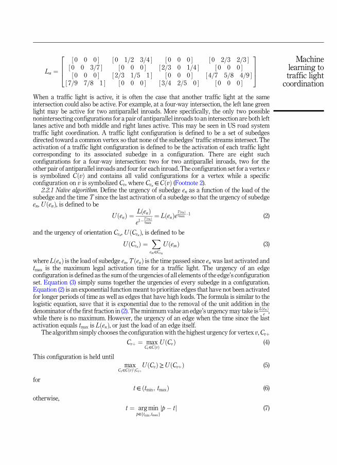
Lα ¼

2664

½ 0 0 0 � ½ 0 1=2 3=4 � ½ 0 0 0 � ½ 0 2=3 2=3 �½ 0 0 3=7 � ½ 0 0 0 � ½ 2=3 0 1=4 � ½ 0 0 0 �½ 0 0 0 � ½ 2=3 1=5 1 � ½ 0 0 0 � ½ 4=7 5=8 4=9 �

½ 7=9 7=8 1 � ½ 0 0 0 � ½ 3=4 2=5 0 � ½ 0 0 0 �

3775

When a traffic light is active, it is often the case that another traffic light at the sameintersection could also be active. For example, at a four-way intersection, the left lane greenlight may be active for two antiparallel inroads. More specifically, the only two possiblenonintersecting configurations for a pair of antiparallel inroads to an intersection are both leftlanes active and both middle and right lanes active. This may be seen in US road systemtraffic light coordination. A traffic light configuration is defined to be a set of subedgesdirected toward a common vertex so that none of the subedges’ traffic streams intersect. Theactivation of a traffic light configuration is defined to be the activation of each traffic lightcorresponding to its associated subedge in a configuration. There are eight suchconfigurations for a four-way intersection: two for two antiparallel inroads, two for theother pair of antiparallel inroads and four for each inroad. The configuration set for a vertex vis symbolized CðvÞ and contains all valid configurations for a vertex while a specificconfiguration on v is symbolized Cv, where Cvn ∈CðvÞ (Footnote 2).

2.2.1 Naı€ve algorithm. Define the urgency of subedge en as a function of the load of thesubedge and the time T since the last activation of a subedge so that the urgency of subedgeen, UðenÞ, is defined to be

UðenÞ ¼ LðenÞe1 –

TðenÞtmax

¼ LðenÞeTðenÞtmax

–1 (2)

and the urgency of orientation Cvn, UðCvnÞ, is defined to be

UðCvnÞ ¼Xem∈Cvn

UðemÞ (3)

where LðenÞ is the load of subedge en,TðenÞ is the time passed since en was last activated andtmax is the maximum legal activation time for a traffic light. The urgency of an edgeconfiguration is defined as the sum of the urgencies of all elements of the edge’s configurationset. Equation (3) simply sums together the urgencies of every subedge in a configuration.Equation (2) is an exponential function meant to prioritize edges that have not been activatedfor longer periods of time as well as edges that have high loads. The formula is similar to thelogistic equation, save that it is exponential due to the removal of the unit addition in thedenominator of the first fraction in (2). Theminimumvalue an edge’s urgencymay take is LðenÞ

e,

while there is no maximum. However, the urgency of an edge when the time since the lastactivation equals tmax is LðenÞ, or just the load of an edge itself.

The algorithm simply chooses the configuration with the highest urgency for vertex v,CvþCvþ ¼ max

Cv∈CðvÞUðCvÞ (4)

This configuration is held until

maxCv∈CðvÞnCvþ

UðCvÞ≥UðCvþÞ (5)

for

t ∈ ðtmin; tmaxÞ (6)

otherwise,

t ¼ argminp∈ftmin;tmaxg

jp� tj (7)

Machinelearning totraffic lightcoordination

where tmin is the minimum legal activation time for a traffic light. This is so that theconfiguration is activated until the urgency directly before the configuration was activatedequals the urgency of another configuration directly before it was activated, while keeping inmind minimum and maximum green light length rules. The algorithm is conducted in realtime, so there is no need for a model of unload speed; rather, real-time data is used and therules aforementioned are used when monitoring load. In fact, because the algorithm isconducted in real time, the modeling of outflow may be safely ignored in its entirety as nomodeling is required when real-time data is available. As a result, it suffices to only consideredge and subedge inflow in the algorithm.

2.2.2 Cumulative algorithm.The previously detailed algorithm is a naı€ve algorithm similarto those of various systems used to coordinate traffic lights in that these algorithms fail toconsider future traffic and how to best prevent traffic density from increasing through futurepredictions. As may be obvious, the intersection road-induced graph fails to consider thenumber of vehicles at places such as department stores or office buildings because

(1) taking those places into account would result in an overly complex graph and “road”system and

(2) violating the conservation of graph flow allows for generalized predictions to bemadeby relegating the entrances and exits of vehicles into and from buildings to negativeand positive edge flow.

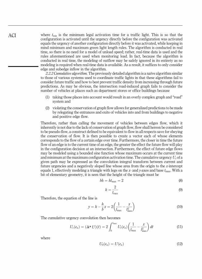
Therefore, rather than calling the movement of vehicles between edges flow, which itinherently is not due to the lack of conservation of graph flow, flow shall hereon be consideredto be pseudo-flow, a construct defined to be equivalent to flow in all respects save for obeyingthe conservation of flow. It is then possible to create a vector each of whose elementscorresponds to the flow of a certain edge over time. Furthermore, the closer in time the futureflow of an edge is to the current time of an edge, the greater the effect the future flowwill playin the configuration decision at an intersection. Furthermore, the effect of future edge flowsmay be modeled using a bounded sine function whose maximum occurs at the current timeandminimum at themaximum configuration activation time. The cumulative urgencyUc of agiven path may be expressed as the convolution integral transform between current andfuture urgencies and a negatively sloped line whose area from the origin to the x-interceptequals 1, effectively modeling a triangle with legs on the x- and y-axes and base tmax. With abit of elementary geometry, it is seen that the height of the triangle must be

bh ¼ htmax ¼ 2 (8)

h ¼ 2

tmax

(9)

Therefore, the equation of the line is

y ¼ h� h

bx ¼ 2

�1

tmax

� x

t2max

�(10)

The cumulative urgency convolution then becomes

UcðenÞ ¼ ðΔ*UÞðtÞ ¼ 2

Z tmax

0

UtðenÞ�

1

tmax

� x

t2max

�dt (11)

where

U0ðenÞ ¼ UðenÞ (12)

ACI

and

UtðenÞ ¼ LðentÞe1–TðenÞtmax (13)

where ent is the subedge en at time t.Future flow is predicted using a recurrent neural network (RNN) due to the fact that the

current inflow of a directed edge both is roughly periodic in nature and is a product of previousinflows. For example, it is to be expected that certain roadswill see above-average inflows duringrush hour. Similarly, inflows cannot stay high for long periods of time if the inflows of otherroads have been lowbecause the low inflows of other roadsmeans that the roadwith high inflowis getting saturated and is approaching capacity. The RNN used is to decrease computationtimes, simplify calculations and take into account the inherently discrete nature of traffic lighttiming, a single triply nested long short-termmemory (NLSTM) unit [9]. Nested LSTMs presenta solution to this problem by replacing the long-term memory unit of an LSTM with anotherLSTM, thus increasing the long-termmemory span of the nested LSTM. The reason behind theuse of a triply nested LSTM rather than a conventional LSTM [10] is that the time steps used inthemodel occur on the order ofminutes, but patterns in traffic inflow often occur on the order ofdays, months or even years. One oft-noted problem with vanilla LSTMs is that although theyare competent at recognizing patterns occurring over hundreds of time steps, their long-termmemory fails to remember patterns spanning thousands or more time steps [11, 12]. Becausethere are around 365 � 24 � 60 � 60 ¼ 32; 850; 000 minutes or time steps in a year, which isclose to log500 32; 850; 000≈ 2:7784≈ 3magnitudes greater than a single LSTM can handle, itis necessary to have at least three levels of LSTMs to properly account for patterns spanninglong ranges of time. Due to the discreteness of both the RNN and the configuration activations,the cumulative urgency integral must be transformed into a discrete convolution summation

UcðenÞ ¼ ðΔ*UÞ½t� ¼ 2Xtmax

t¼0

�UtðenÞ

�1

tmax

� x

t2max

��(14)

The cumulative urgency is substituted for the naı€ve urgency when relegating intersectionconfiguration so that Cvþ becomes

Cvþ ¼ maxCv∈CðvÞ

UcðCvÞ (15)

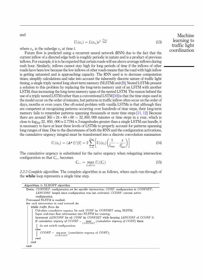
2.2.3 Complete algorithm. The complete algorithm is as follows, where each run-through ofthe while loop represents a single time step.

Machinelearning totraffic lightcoordination

The prediction portion of the algorithm is governed by the NLSTM, which has trained onpast traffic inflow data; the assumption is made that the more traffic data has been trainedupon, the more comprehensive the patterns the NLSTM learns are. At any moment, theNLSTM is able to predict future inflows by outputting predictions when given current orpredicted future inflows. It is through this method that the NLSTM is able to predict inflowstens of time steps into the future.

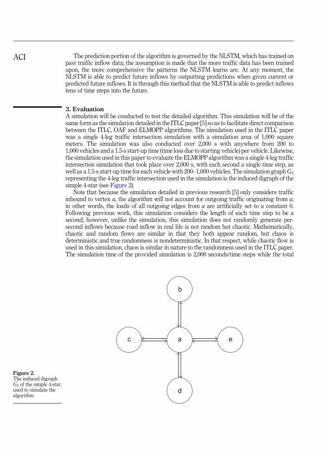
3. EvaluationA simulation will be conducted to test the detailed algorithm. This simulation will be of thesame form as the simulation detailed in the ITLC paper [5] so as to facilitate direct comparisonbetween the ITLC, OAF and ELMOPP algorithms. The simulation used in the ITLC paperwas a single 4-leg traffic intersection simulation with a simulation area of 1,000 squaremeters. The simulation was also conducted over 2,000 s with anywhere from 200 to1,000 vehicles and a 1.5-s start-up time (time loss due to starting vehicle) per vehicle. Likewise,the simulation used in this paper to evaluate the ELMOPP algorithmwas a single 4-leg trafficintersection simulation that took place over 2,000 s, with each second a single time step, aswell as a 1.5-s start-up time for each vehicle with 200–1,000 vehicles. The simulation graphGS

representing the 4-leg traffic intersection used in the simulation is the induced digraph of thesimple 4-star (see Figure 2).

Note that because the simulation detailed in previous research [5] only considers trafficinbound to vertex a, the algorithm will not account for outgoing traffic originating from a;in other words, the loads of all outgoing edges from a are artificially set to a constant 0.Following previous work, this simulation considers the length of each time step to be asecond; however, unlike the simulation, this simulation does not randomly generate per-second inflows because road inflow in real life is not random but chaotic. Mathematically,chaotic and random flows are similar in that they both appear random, but chaos isdeterministic and true randomness is nondeterministic. In that respect, while chaotic flow isused in this simulation, chaos is similar in nature to the randomness used in the ITLC paper.The simulation time of the provided simulation is 2,000 seconds/time steps while the total

a

b

c

d

e

Figure 2.The induced digraphGS of the simple 4-star,used to simulate thealgorithm

ACI

number of vehicles is 200–1,000, with a set of 30 trials conducted. Therefore, a periodic inflowfunction will be enacted to better simulate real-world traffic inflow. This inflow function is afour-dimensional autonomous hyperchaotic system modeled off the Lorenz attractor asdescribed in the hyperchaotic system paper [13]. That system of differential equations (seeappendix) exhibits chaotic behavior, which models the real world.

To conform to the simulation used, the hyperchaotic system will be normalized bydividing the values generated at each time step by the integral of the system over the interval[0, 2,000], then will be scaled by a random integer over the interval [200, 1,000]. This results inchaotic inflow with, following previous work, a total number of incoming vehicles between200 and 1,000. The capacity of each road was not given in the original paper’s simulationdescription; therefore, the capacity of every inroad to a is set to be a constant 1,000. Note thatthe value of the capacity itself may be arbitrarily positive because all that matters is that thecapacities themselves are equal across all edges, as only capacity ratios are considered as canbe seen from the urgency formula. The simulation previously described also contains otherinformation, such as the area over which the simulation is conducted, variables that areextraneous to this simulation as ELMOPP does not require these variables.

The LSTM used in the simulation will not be a triply nested LSTM, but will instead be avanilla LSTM (one may consider this to be a singly nested LSTM) because the hyperchaoticsystem will be timewise scaled down to produce patterns over time intervals ranging fromminutes to hours due simply to the length of the simulation detailed in the ITLC paper [5](around 33 min over 2,000 single-second time steps). In other words, the LSTM used in thesimulation will be a vanilla LSTM simply because the timescale of the simulation ismagnitudes shorter than the timescale of real-world traffic patterns; therefore, a triply nestedLSTM is not needed as the timescale it handles dwarfs the timescale of the simulation and ismore computation-intensive than the better-suited LSTM (better-suited only for thesimulation). As a result, the RNN used will not need to be able to handle large timescales.More details on the simulation are provided in the appendix.

The results from the simulation were collected and compared against the results from theITLC andOAF simulations [5], as shown in the following plot. The data collectedwere plottedagainst the results of the ITLC and OAF algorithms.

200 400 600 800 1,0001

1.2

1.4

1.6

1.8

2

2.2

2.4

Number of travelling vehicles

Throughput(vehiclespersecond)

Throughput vs. travelling vehicle count of all three algorithms

ELMOPP

ITLC

OAF

Furthermore, an independent samples t-test was conducted for each pair of algorithms.The mean of the ELMOPP algorithm is 2.09133 and the standard deviation 0.158824. Themean of the ITLC algorithm is 1.83414 with a standard deviation of 0.080730. Finally, the

Machinelearning totraffic lightcoordination

mean of the OAF algorithm is 1.12108 with a pooled standard deviation of 0.063498. Thirtytrials were conducted for each data point provided for every algorithm. Three independentsamples t-tests were conducted for every pair of algorithms. It was assumed that the datadistributions and the variances for each algorithm were different when conducting the tests,supported by the calculated standard deviations. The null hypothesis was that the means ofthe distributions were equal while the alternate hypothesis was that the greater mean wasactually greater than the lesser mean. Therefore, the t-test was one-sided. Finally, the degreesof freedomwere set to 298 for each test as there were 150 data points for each data set and thelevel of significance was set to 0.05. The results of the t-tests are shown further.

At the 95% confidence level, it is seen that the alternate hypothesis is supported for eachpair of algorithms. This, coupled with the algorithm’s means in order from greatest to leastas ELMOPP, ITLC and OAF, supports the hypothesis that ELMOPP exhibits a higherthroughput than both ITLC and OAF. Surprisingly, the calculated t-value for the ITLCv. OAF test is the greatest of all calculated t-values. This is because, even though thedifference of means for this test is smaller than the difference of means for the ELMOPP v.OAF, the variance for the ITLC data set is also smaller than the variance for the ELMOPPdata set.

4. Applications and further researchApplications of the novel ELMOPP algorithm are varied in scope. As a traffic managementalgorithm built to keep traffic flow in road systems as high as possible, ELMOPP could beused on practically any road system. ELMOPP would be especially useful in places that donot have access to GPS systems or aren’t able to pay for extreme renovations to road systemsas would be required by systems such as SCATS or SCOOT. This includes places such ascities with low funds or towns with minimal extra resources. In fact, ELMOPP could beapplied to any road system that needs a traffic management system quickly as it isstraightforward to implement and requires practically no physical modifications to existingroad systems. The observed increase in throughput shown by ELMOPP in comparison withITLC and OAF is beneficial for another reason: environmental impact. Increased trafficcongestion has been shown to correlate with lower ambient air quality and has even beenlinked to trends in increasingmortality. Hazards associatedwith traffic congestion have beenshown to be related to travel time and rush hour length, among others [14]. As ELMOPPseems to show a higher throughput than ITLC and OAF, it is safe to say that travel time willbe reduced as more vehicles at any given moment are traveling to their destination forELMOPP than for either of the other two algorithms. Furthermore, ELMOPPwas specificallycreated to predict and mitigate future traffic, something that has immediately obviousimplications for rush hour traffic. This further supports the application of ELMOPP todecreasing environmental impact and positively impacting people’s health.

Further research on the subject of traffic management algorithms would likely involvedifferent methods of approaching and describing the problem. ITLC used algebra and basiccombinatorics to create what was a very loose description of road systems; ELMOPP usedgraph theory and linear algebra to describe and optimize traffic. There are other, potentiallymore scalable, methods of describing traffic flow. Further research by the researcher would

Test Calculated t-value Table t-value Significance

t-test: ELMOPP v. ITLC 17.6799 1.6500 Significantt-test: OAF v. ELMOPP 69.4727 1.6500 Significantt-test: ITLC v. OAF 85.0275 1.6500 Significant

ACI

likely be focused on the avenues of other methods of predicting traffic flow, such as throughvanilla artificial neural networks (ANNs) or graph convolutional networks (GCNs). One specificvenue for further research could be real-world testing by implementingELMOPP for a physicalroad system and comparing its performance to other traffic management algorithms. Another,more comprehensive, method of further research might involve developing a suite of networktests to cover a range of situations such as alternating heavy and light traffic flow, variousintersection types, traffic management algorithms applied to simulated road networks ratherthan individual intersections and counting roads with varying speed limits.

5. ConclusionThis paper outlined a novel traffic management algorithm named ELMOPP that employedgraph theory and nested LSTMs. The ELMOPP algorithm assumes that current traffic flowis correlated with past traffic flow and that traffic cameras are able to collect data that can beused to determine incoming traffic parameters. In contrast to real-time traffic optimization,the ELMOPP algorithm attempts to optimize traffic across time by searching for the mostefficient traffic flow using machine-learned traffic patterns to predict future traffic(Footnote 3). The ability of this algorithm to consider traffic predictions in its managementdecisions renders it significantly more effective than the ITLC and OAF algorithms whileusing fewer metrics. The present study is restricted only to simulations to address trafficmanagement performance; physical, real-world testing will demand further research.

Notes

1. The load of an edge is artificially set to 0 when the capacity of an edge is 0 as it is not possible for anyvehicles to travel on that edge. In setting the edge load to 0when the capacity is 0, the urgency of thatedge becomes 0, preventing so-called “dead” edges from having any effect on configuration urgency.

2. Note that, although four-road intersections are most often mentioned in this paper, intersections ofany possible number occur in the real world. Four-road intersections are used as examples heresimply because they are common, it is easy for audiences to understand the ELMOPP algorithmthrough easily relatable examples, and because the simulation used to test the algorithm uses afour-road intersection in keeping with the ITLC paper [5]. However, the idea of a configuration isvalid for all types of intersections. All that must be done is to define the configuration set as the set ofall possible configurations.

3. Supplementary material related to this paper, including this paper’s appendix, may be found withinthe following GitHub repository: https://github.com/meeeeee/ELMOPP-ACI

References

1. Clark L. Traffic signals: a brief history. 2019. Available at: https://magazine.wsu.edu/web-extra/traffic-signals-a-brief-history/.

2. New South Wales Government. SCATS: Sydney coordinated adaptive traffic system. 2011.Available at: https://www.qtcts.com.au/media/512152-RTA532_SCATS_A4_Product_Brochure_07.pdf.

3. Bretherton RD. Scoot urban traffic control system — Philosophy and evaluation. IFACProceedings Volumes 23.2. IFAC/IFIP/IFORS Symposium on Control, Computers,Communications in Transportation, Paris, France, 19-21 September; 1990: 237-39. ISSN: 1474-6670. doi: 10.1016/S1474-6670(17)52676-2. Available at: http://www.sciencedirect.com/science/article/pii/S1474667017526762.

4. Hemakumar V, Nazini H. Optimized traffic signal control system at traffic intersections usingVANET. IET Chennai Fourth International Conference on Sustainable Energy and IntelligentSystems (SEISCON 2013). 2013: 305-12.

Machinelearning totraffic lightcoordination

5. Bani Younes M, Boukerche A. An intelligent traffic light scheduling algorithm through VANETs.39th Annual IEEE Conference on Local Computer Networks Workshops. 2014: 637-42.

6. Wahab L, Jiang H. A comparative study on machine learning based algorithms for prediction ofmotorcycle crash severity. PloS One. 2019; 14(4): e0214966.

7. Krishna KVSA, Abhishek K, Allam S, Shantala Devi P, Gopala Krishna S. Smart traffic analysisusing machine learning. International Journal of Engineering and Advanced Technology (IJEAT)8 (5S 2019). IFAC/IFIP/IFORS Symposium on Control, Computers, Communications inTransportation. Paris, France: 19-21 September; 2019: 199-202. ISSN: 2249-8958.

8. Liu F, Zeng Z, Jiang R. A video-based real-time adaptive vehicle-counting system for urban roads.PloS One. 2017; 12(11): 1-16. doi: 10.1371/journal.pone.0186098.

9. Ruben Antony Moniz J, Krueger D. Nested LSTMs. Proceedings of the Ninth Asian Conference onMachine Learning. Ed. by Min-Ling Z, Yung-Kyun N. 77. Proceedings of Machine LearningResearch. PMLR. 2017: 530-44. Available at: http://proceedings.mlr.press/v77/moniz17a.html.

10. Hochreiter S, Schmidhuber J. Long short-term memory. Neural Computation 450-451. 1997: 307-16.doi: 10.1016/j.scitotenv.2013.01.074.

11. Greff K, et al. LSTM: a search space odyssey. IEEE Transactions on Neural Networks andLearning Systems. 2017; 28(10): 2222-32.

12. Hochreiter S. The vanishing gradient problem during learning recurrent neural nets and problemsolutions. International Journal of Uncertainty, Fuzziness and Knowledge-Based Systems. 1998.doi: 10.1142/S0218488598000094.

13. Zhang G, et al. On the dynamics of new 4D Lorenz-type chaos systems. Advances in DifferenceEquations. 2017; 1. doi: 10.1186/s13662-017-1280-5.

14. Zhang K, Batterman S. Air pollution and health risks due to vehicle traffic. Science of the TotalEnvironment. 2013; 450-451: 307-316. doi: 10.1016/j-scitotenv.2013.01.074.

15. Wolfermann A, Alhajyaseen W, Nakamura H. Modeling speed profiles of turning vehicles atsignalized intersections. 2011.

16. Cascetta E. Transportation systems engineering: theory and methods. Chap. 3: Traffic StreamModels. 2014: ISBN: 9781475768732.

Appendix

Hyperchaotic System Inflow SimulationsThe hyperchaotic system governing inflow dynamics for the simulation was

ðx; y; z; wÞ :¼

8>>>>>>>>>>>><>>>>>>>>>>>>:

dx

dt¼ aðy� xÞ � ew;

dy

dt¼ xz� hy;

dz

dt¼ b� xy� cz;

dw

dt¼ ky� dw

(16)

where “a, b, c, d, e, h are positive parameters of system” [13] and with the specific attractor a5 5, b5 20,c5 1, d5 0.1, e5 20.6, h5 1 and k5 0.1. As stated by the paper, the largest Lyapunov exponent of theattractor above is 0.24. As a result, the Lyapunov time of the system is 1=0:24 ≈ 4:167. Because eachsystem time step is 0.01, the Lyapunov time expressed in time steps is 4:167=0:01 ≈ 417, which amounts

ACI

to 417=60 ≈ 6:95min, far greater than any reasonablemaximum traffic light activation time. As a result,the cumulative urgency formula is not expected to significantly diverge from the true chaoticdistribution as the Lyapunov time is far greater than any expected result.

The system was solved by using the Runge–Kutta family’s Euler method with a step size of 0.01over ½0; 2000� by treating the system as the derivative of a vector-valued function.

Euler’s method allows for discrete approximations of differential equations. It states that forfunction y and its derivative y0,

hnþ1 ¼ hn þ h0 ðtnÞΔn (17)

This may be extended to vector-valued functions, such as the previously described hyperchaotic system[13], where

h ¼

2664x

y

z

w

3775; h

0 ¼

2664aðy� xÞ � ew

xz� hy

b� xy� cz

ky� dw

3775 (18)

and Δn ¼ 0:01.The system was normalized by dividing the system by the L1 norm of its integral over [0, 2,000],

then scaling it up by a factor of 800. This effectively modeled chaotic vehicle inflow so that the totalinflow over the 2,000 timestepswas 800 vehicles. The integral of the solutionwas calculated by summingall of the data points calculated through Euler.

Because the step size was 0.01 and the stiffness ratio (ignoring the eigenvalue of 0) was−7:56=0:23 ≈ − 32:8695, which is not significantly less than –1, it is safe to say that the system isnonstiff for the estimation technique used.

LSTM Prediction ModelThe LSTM prediction model trained on 10,000 data points. The data was generated by choosing arandom real vector v∈R4 so that v is a vector randomly sampled from the four-dimensional hypercubewhose boundaries are defined by the fourfold Cartesian product ff0; 1g3f0; 1g3f0; 1g3f0; 1gg. TheLSTM’s training data was split 80–20 as traditionally split when training and testing data for machinelearningmodels. The first 8,000 data points were used only trainingwhile the last 2,000 points were usedfor simulation. Every data point in the last 2,000 points was trained pointwise on the LSTM as a single-sample batch.

The LSTM itself consisted of 16 units (determined empirically through tests over different ranges ofunits to be the optimal number of units to facilitate low errors while preventing overfitting for thespecific attractor used) andwas trained over 100 epochs with a batch size of ten samples using theAdamoptimizer with a mean squared error loss function.

Traffic Intersection SimulationFew details were given on the ns2 map used in the ITLC paper [5]; as a result, some assumptions weremade about the simulation. The turning speed was set at a constant 10 m per second, chosen from thethorough analysis done in MODELING SPEED PROFILES OF TURNING VEHICLES ATSIGNALIZED INTERSECTIONS [15]. Furthermore, the outflow rate (q) was calculated using anumerical Greenshield model [16] to be

q ¼ kvf

�1� k

kj

�(19)

where k is the density, vf is the free-flow speed and kj is the jam density. The capacity of each street wasset to 1,000 vehicles. Each inroad was initialized to a load of 200 vehicles with the total vehicle inflowover the 2,000-s testing interval being 800, with a resulting 4,000 vehicles total and an average of

Machinelearning totraffic lightcoordination

1,000 vehicles per inroad, only accomplished if all 4,000 vehicles flow out over the 2,000-s interval.The capacity for each inroad was set to 1,000 with a jam density of 1.

Corresponding authorFareed Sheriff can be contacted at: fareedsheriff@gmail.com

For instructions on how to order reprints of this article, please visit our website:www.emeraldgrouppublishing.com/licensing/reprints.htmOr contact us for further details: permissions@emeraldinsight.com

ACI