ELLIPTIC CURVES AND THEIRAPPLICATIONS IN CRYPTOGRAPHY

A Thesis Presented tothe Faculty of the Graduate School

University of Missouri

In Partial Fulfillmentof the Requirements for the Degree

Master of Science

byMICHAEL PEMBERTON

Dr. William Banks, Thesis Supervisor

DECEMBER 2009

The undersigned, appointed by the Dean of the Graduate School,have examined the thesis entitled

ELLIPTIC CURVES AND THEIRAPPLICATIONS IN CRYPTOGRAPHY

Presented by Michael Pemberton

A candidate for the degree of Master of Science

And hereby certify that in their opinion it is worthy of acceptance.

Professor William Banks

Professor Zhenbo Qin

Professor Youssef Saab

ACKNOWLEDGEMENTS

First of all, I would like to thank my thesis advisor, William Banks, for his

support and understanding throughout the process of completing this thesis. His

encouragement and guidance has helped me realize my passion for elliptic curves

and cryptography and to pursue a career in the field.

To those professors who helped me begin my journey in advanced mathematics,

thank you for all your patience and support. You have helped me to develop

my love for mathematics and have inspired me to pass on my passion. In particular,

would like to thank Ian Aberbach and Zhenbo Qin, for their numerous courses

and seminars that I was privileged to enroll in while at Mizzou.

I would also like to thank my family and friends for all their unwavering

support, love, patience, and encouragement. To my parents for all their love and

inspiration in all that I do, and without their help, none of my accomplishments

would be possible.

ii

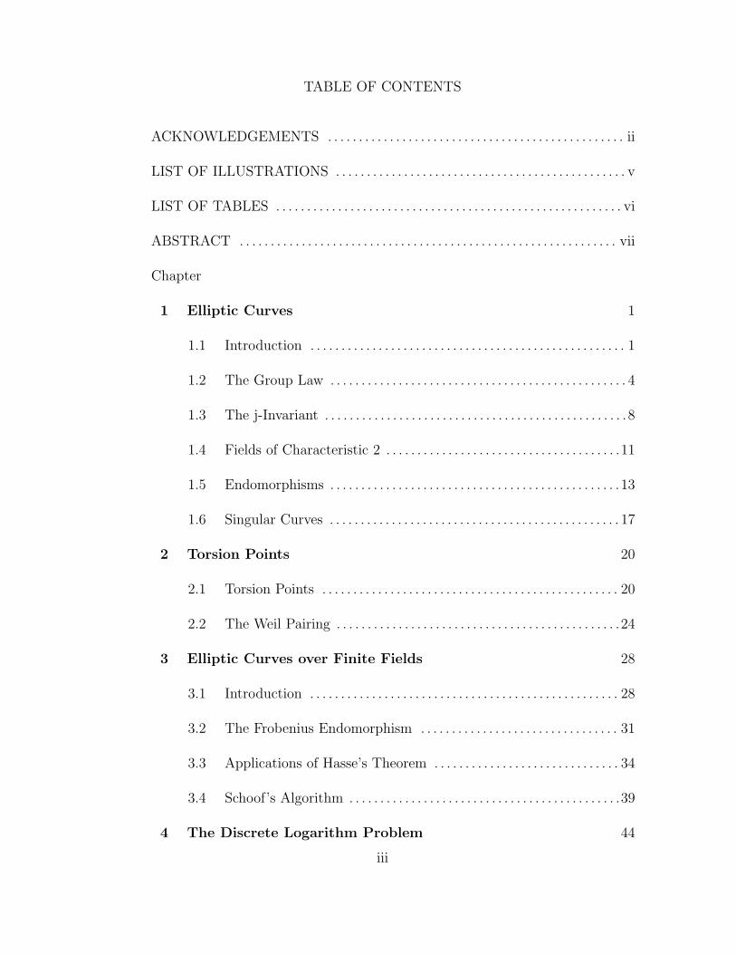
TABLE OF CONTENTS

ACKNOWLEDGEMENTS . . . . . . . . . . . . . . . . . . . . . . . . . . . . . . . . . . . . . . . . . . . . . . . . ii

LIST OF ILLUSTRATIONS . . . . . . . . . . . . . . . . . . . . . . . . . . . . . . . . . . . . . . . . . . . . . . . v

LIST OF TABLES . . . . . . . . . . . . . . . . . . . . . . . . . . . . . . . . . . . . . . . . . . . . . . . . . . . . . . . . vi

ABSTRACT . . . . . . . . . . . . . . . . . . . . . . . . . . . . . . . . . . . . . . . . . . . . . . . . . . . . . . . . . . . . . vii

Chapter

1 Elliptic Curves 1

1.1 Introduction . . . . . . . . . . . . . . . . . . . . . . . . . . . . . . . . . . . . . . . . . . . . . . . . . . . 1

1.2 The Group Law . . . . . . . . . . . . . . . . . . . . . . . . . . . . . . . . . . . . . . . . . . . . . . . . 4

1.3 The j-Invariant . . . . . . . . . . . . . . . . . . . . . . . . . . . . . . . . . . . . . . . . . . . . . . . . . 8

1.4 Fields of Characteristic 2 . . . . . . . . . . . . . . . . . . . . . . . . . . . . . . . . . . . . . .11

1.5 Endomorphisms . . . . . . . . . . . . . . . . . . . . . . . . . . . . . . . . . . . . . . . . . . . . . . .13

1.6 Singular Curves . . . . . . . . . . . . . . . . . . . . . . . . . . . . . . . . . . . . . . . . . . . . . . . 17

2 Torsion Points 20

2.1 Torsion Points . . . . . . . . . . . . . . . . . . . . . . . . . . . . . . . . . . . . . . . . . . . . . . . . 20

2.2 The Weil Pairing . . . . . . . . . . . . . . . . . . . . . . . . . . . . . . . . . . . . . . . . . . . . . .24

3 Elliptic Curves over Finite Fields 28

3.1 Introduction . . . . . . . . . . . . . . . . . . . . . . . . . . . . . . . . . . . . . . . . . . . . . . . . . . 28

3.2 The Frobenius Endomorphism . . . . . . . . . . . . . . . . . . . . . . . . . . . . . . . . 31

3.3 Applications of Hasse’s Theorem . . . . . . . . . . . . . . . . . . . . . . . . . . . . . . 34

3.4 Schoof’s Algorithm . . . . . . . . . . . . . . . . . . . . . . . . . . . . . . . . . . . . . . . . . . . .39

4 The Discrete Logarithm Problem 44

iii

4.1 The Index Calculus . . . . . . . . . . . . . . . . . . . . . . . . . . . . . . . . . . . . . . . . . . . 45

4.2 Attacks on Discrete Logs . . . . . . . . . . . . . . . . . . . . . . . . . . . . . . . . . . . . . . 48

4.2.1 Baby Step, Giant Step . . . . . . . . . . . . . . . . . . . . . . . . . . . . . . . . 48

4.2.2 Pollard’s ρ Method . . . . . . . . . . . . . . . . . . . . . . . . . . . . . . . . . . . . 49

4.3 Attacks with Pairings . . . . . . . . . . . . . . . . . . . . . . . . . . . . . . . . . . . . . . . . . 52

5 Elliptic Curve Cryptography 56

5.1 Basic Setup . . . . . . . . . . . . . . . . . . . . . . . . . . . . . . . . . . . . . . . . . . . . . . . . . . . 56

5.2 Diffie-Hellman Key Exchange . . . . . . . . . . . . . . . . . . . . . . . . . . . . . . . . . 57

5.3 ElGamal Public Key Encryption . . . . . . . . . . . . . . . . . . . . . . . . . . . . . . 59

5.4 ElGamal Digital Signatures . . . . . . . . . . . . . . . . . . . . . . . . . . . . . . . . . . . 60

5.5 Elliptic Curve Analogue of RSA . . . . . . . . . . . . . . . . . . . . . . . . . . . . . . . 63

6 Applications in Number Theory 66

6.1 Factoring Using Elliptic Curves . . . . . . . . . . . . . . . . . . . . . . . . . . . . . . . 66

6.2 Primality Testing . . . . . . . . . . . . . . . . . . . . . . . . . . . . . . . . . . . . . . . . . . . . . 69

APPENDIX

A Projective Space and the Point at Infinity 72

BIBLIOGRAPHY . . . . . . . . . . . . . . . . . . . . . . . . . . . . . . . . . . . . . . . . . . . . . . . . . . . . . . . . 75

iv

LIST OF ILLUSTRATIONS

Figure Page

1.1: Basic Forms of Elliptic Curves over R . . . . . . . . . . . . . . . . . . . . . . . . . . . . . . . . . . . . . 2

1.2: Addition on Elliptic Curves . . . . . . . . . . . . . . . . . . . . . . . . . . . . . . . . . . . . . . . . . . . . . . . 5

4.1: Pollard’s ρ Method . . . . . . . . . . . . . . . . . . . . . . . . . . . . . . . . . . . . . . . . . . . . . . . . . . . . . . 50

v

LIST OF TABLES

Table Page

3.1: Points on y2 = x3 + x+ 1 over F5 . . . . . . . . . . . . . . . . . . . . . . . . . . . . . . . . . . . . . . . . 29

vi

ELLIPTIC CURVES AND THEIRAPPLICATIONS IN CRYPTOGRAPHY

Michael Pemberton

Dr. William Banks, Thesis Supervisor

ABSTRACT

In 1985, Koblitz and Miller proposed elliptic curves to be used for public

key cryptosystems. This present thesis examines the role of elliptic curves on

cryptography and basic problems involving implementation and security of some

elliptic curve cryptosystems. Some of the aspects we are concerned with include:

• Methods to determine the number of points on an elliptic curve over a

finite field

• Implementation of cryptosystems based on the discrete logarithm problem

for elliptic curves defined over a finite field

• Examine an elliptic curve analogue of the RSA cryptosystem

We provide answers to these and discuss a number of applications for number

theory, such as factorization and primality testing.

vii

Chapter 1

Elliptic Curves

In this chapter we provide motivation for the study of elliptic curves in

cryptography. We begin with basic forms in which an elliptic curve may be

expressed, then discuss the group law, which provides the foundation for all

cryptographic applications. We then provide a method to classify all elliptic curves

up to isomorphism and conclude with a discussion of endomorphisms to provide

the background needed for Hasse’s theorem in Chapter 3.

1.1 Introduction

Let K be a field. For example, K can be the prime field Fp, where p is a prime

number, a finite extension field Fpn of Fp, for some n ≥ 1, or one of the fields

of rational, real, or complex numbers.

Definition 1.1.1. An elliptic curve E over a field K, denoted E(K), is defined by

the Weierstrauss equation for E,

y2 = x3 + ax+ b (1.1)

where a, b ∈ K. The number of points on E is called the cardinality of E and is

denoted #E(K), or simply #E.

1

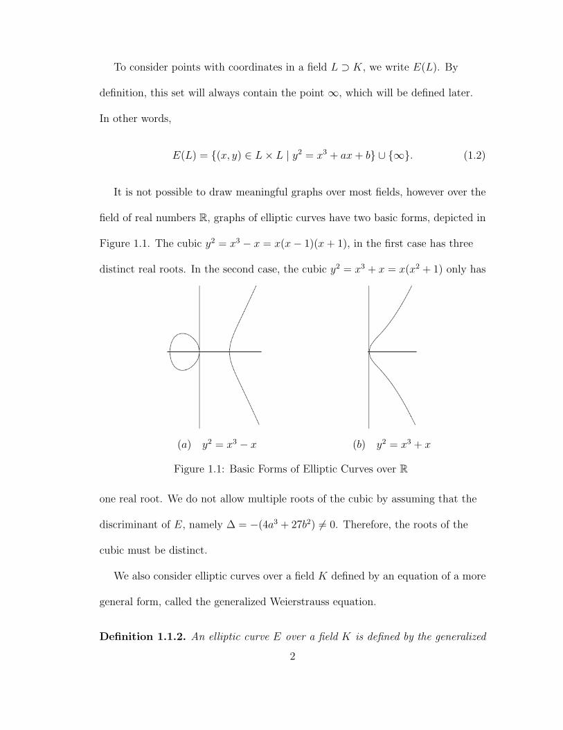
To consider points with coordinates in a field L ⊃ K, we write E(L). By

definition, this set will always contain the point ∞, which will be defined later.

In other words,

E(L) = {(x, y) ∈ L× L | y2 = x3 + ax+ b} ∪ {∞}. (1.2)

It is not possible to draw meaningful graphs over most fields, however over the

field of real numbers R, graphs of elliptic curves have two basic forms, depicted in

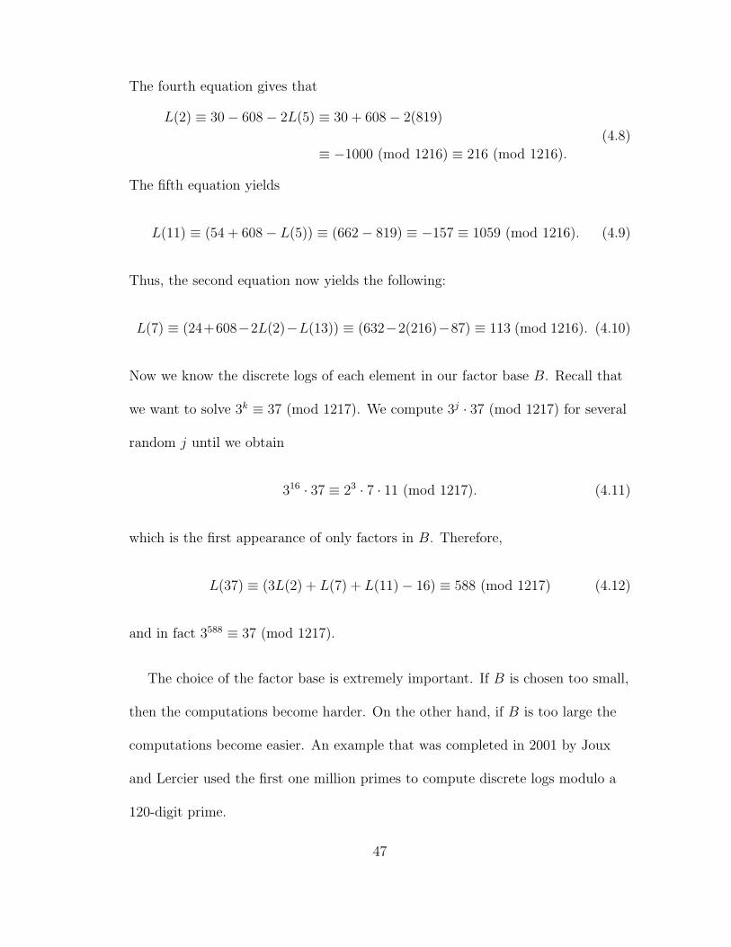
Figure 1.1. The cubic y2 = x3 − x = x(x− 1)(x+ 1), in the first case has three

distinct real roots. In the second case, the cubic y2 = x3 + x = x(x2 + 1) only has

(a) y2 = x3 − x (b) y2 = x3 + x

Figure 1.1: Basic Forms of Elliptic Curves over R

one real root. We do not allow multiple roots of the cubic by assuming that the

discriminant of E, namely ∆ = −(4a3 + 27b2) 6= 0. Therefore, the roots of the

cubic must be distinct.

We also consider elliptic curves over a field K defined by an equation of a more

general form, called the generalized Weierstrauss equation.

Definition 1.1.2. An elliptic curve E over a field K is defined by the generalized

2

Weierstrauss equation

y2 + a1xy + a3y = x3 + a2x2 + a4x+ a6 (1.3)

where a1, a2, a3, a4, a6 ∈ K.

Elliptic curves of the form (1.3) are useful when working over a field K where

char(K) = 2, 3. However, over a field of char(K) 6= 2, 3, any equation in generalized

Weierstrauss form can be transformed into an equation in Weierstrauss form. If

char(K) 6= 2, then we may divide an equation of the form (1.3) and complete the

square to obtain

(y +

a1x

2+a3

2

)2

= x3 +

(a2 +

a21

4

)x2 +

(a4 +

a1a3

2

)x+

(a2

3

4+ a6

), (1.4)

which can be written as

y21 = x3 + a′2x

2 + a′4x+ a′6 (1.5)

with y1 = y + a1x/2 + a3/2 and for some constants a′2, a′4, a′6. Furthermore, if

char(K) 6= 3, then we can let x1 = x+ a′2/3 and obtain y21 = x3

1 + ax1 + b for some

constants a, b. Therefore, we have arrived at an equation of the form (1.1).

Throughout this paper, we mainly use the Weierstrauss equation or the

generalized Weierstrauss equation for an elliptic curve. However, elliptic curves

arise in various other forms and is worthwhile to discuss these briefly.

The first form is a variant on the Weierstrauss equation called a Legendre equation.

Its advantage is that it allows us to express all elliptic curves over an algebraically

closed field K, with char(K) 6= 2, in terms of one parameter.

3

Proposition 1.1.3. Let K be a field such that char(K) 6= 2 and let

y2 = x3 + ax2 + bx+ c = (x− e1)(x− e2)(x− e3) (1.6)

be an elliptic curve E over K with e1, e2, e3 ∈ K. Let

x1 = (e2 − e1)−1(x− e1), y1 = (e2 − e1)−3/2y, λ =e3 − e1e2 − e1

. (1.7)

Then, λ 6= 0, 1 and y21 = x1(x1 − 1)(x1 − λ).

The parameter λ for E is not unique. In fact, each of

{λ,

1

λ, 1− λ, 1

1− λ,

λ

λ− 1,λ− 1

λ

}(1.8)

yields a Legendre equation for E. They correspond to the six permutations of the

roots e1, e2, e3.

1.2 The Group Law

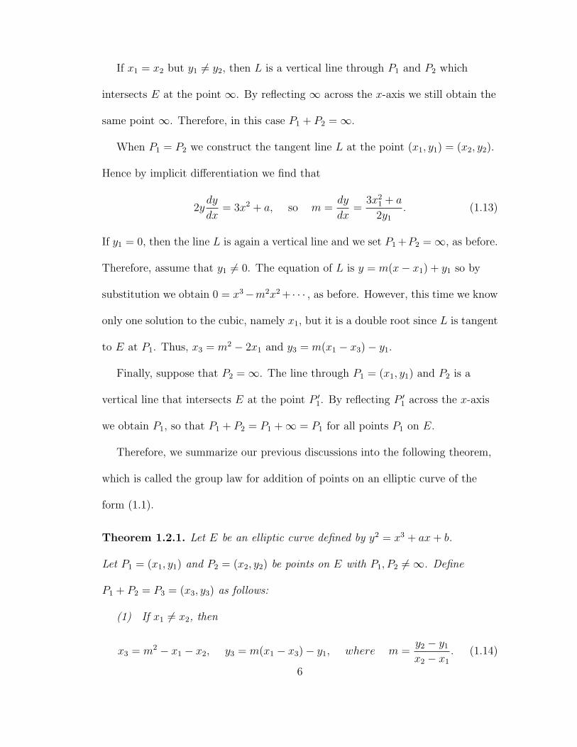
An elliptic curve E defined over a field K can be made into an abelian group

by defining an additive operation on its points. Thus, start with two points

P1 = (x1, y1), P2 = (x2, y2) (1.9)

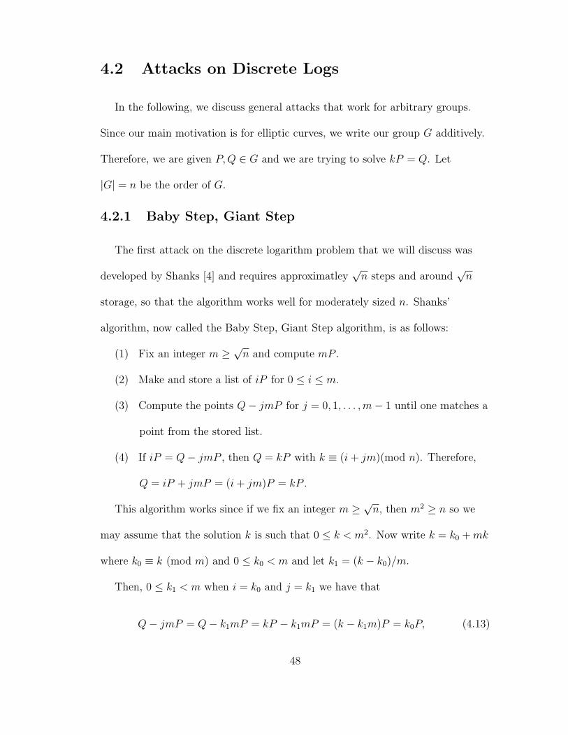
on an elliptic curve E given by y2 = x3 + ax+ b. Define a new point P3 = (x3, y3)

as follows. Draw the line L through the points P1 and P2. The line L intersects E

in a uniquely determined point, which we denote as P ′3. Now reflect the point P ′3

across the x-axis to obtain the point P3. We define P1 + P2 = P3.

4

Figure 1.2: Addition on Elliptic Curves

We will now find explicit formulas to enable us to easily add and subtract

points on an elliptic curve E. The derivation of these formulas uses elementary

analytic geometry, differential calculus to find a tangent line, and a certain amount

of algebraic manipulation. When P1 6= P2 and that neither is ∞, we draw the line

L through P1 and P2. The slope of L is given by

m =y2 − y1

x2 − x1

. (1.10)

Assume that x1 6= x2 so that L is not a vertical line, then the equation of L is

y = m(x− x1) + y1. To find the point of intersection with E, we substitute to get

(m(x− x1) + y1)2 = x3 + ax+ b =⇒ 0 = x3 −m2x2 + · · · . (1.11)

Therefore, the three roots of this cubic correspond to the three points of intersection

of L with E. We already know two solutions, namely x1 and x2. Thus, the third

solution is x = m2 − x1 − x2 and y = m(x− x1) + y1. Therefore, P ′3 = (x, y) and

by reflecting across the x-axis we obtain the point P3 = (x3, y3) where

x3 = m2 − x1 − x2, y3 = m(x1 − x3)− y1. (1.12)

5

If x1 = x2 but y1 6= y2, then L is a vertical line through P1 and P2 which

intersects E at the point ∞. By reflecting ∞ across the x-axis we still obtain the

same point ∞. Therefore, in this case P1 + P2 =∞.

When P1 = P2 we construct the tangent line L at the point (x1, y1) = (x2, y2).

Hence by implicit differentiation we find that

2ydy

dx= 3x2 + a, so m =

dy

dx=

3x21 + a

2y1

. (1.13)

If y1 = 0, then the line L is again a vertical line and we set P1 +P2 =∞, as before.

Therefore, assume that y1 6= 0. The equation of L is y = m(x− x1) + y1 so by

substitution we obtain 0 = x3−m2x2 + · · · , as before. However, this time we know

only one solution to the cubic, namely x1, but it is a double root since L is tangent

to E at P1. Thus, x3 = m2 − 2x1 and y3 = m(x1 − x3)− y1.

Finally, suppose that P2 =∞. The line through P1 = (x1, y1) and P2 is a

vertical line that intersects E at the point P ′1. By reflecting P ′1 across the x-axis

we obtain P1, so that P1 + P2 = P1 +∞ = P1 for all points P1 on E.

Therefore, we summarize our previous discussions into the following theorem,

which is called the group law for addition of points on an elliptic curve of the

form (1.1).

Theorem 1.2.1. Let E be an elliptic curve defined by y2 = x3 + ax+ b.

Let P1 = (x1, y1) and P2 = (x2, y2) be points on E with P1, P2 6=∞. Define

P1 + P2 = P3 = (x3, y3) as follows:

(1) If x1 6= x2, then

x3 = m2 − x1 − x2, y3 = m(x1 − x3)− y1, where m =y2 − y1

x2 − x1

. (1.14)

6

(2) If x1 = x2 but y1 6= y2, then P1 + P2 =∞.

(3) If P1 = P2 and y1 6= 0, then

x3 = m2 − 2x1, y3 = m(x1 − x3)− y1, where m =3x2

1 + a

2y1

. (1.15)

(4) If P1 = P2 and y1 = 0, then P1 + P2 =∞.

Moreover, define P +∞ = P , for all points P on E.

Theorem 1.2.2. The addition of points on an elliptic curve E satisfies:

(1) P1 + P2 = P2 + P1, for all P1, P2 on E.

(2) P +∞ = P , for all P on E.

(3) Given P on E, there exists P ′ on E such that P +P ′ =∞. We will denote

the point P ′ by −P .

(4) P1 + (P2 + P3) = (P1 + P2) + P3, for all P1, P2, P3 on E.

Proof. To prove commutativity of addition, note that the line through two points

P1 and P2 on E is the same line through P2 and P1. The identity property of ∞

holds by definition. For inverses, let P ′ be the reflection of P across the x-axis.

Then P + P ′ =∞.

Finally, we need to prove associativity. This is by far the most subtle and non-

obvious property of the addition of points on E. The associative law can be verified

by calculation with the formulas. There are several cases which makes the proof

rather complicated. See [5], [7] for a proof of the associative law on E.

In other words, the points on E form an additive abelian group with ∞ as the

identity element. Note that if E is defined over a finite field K, then there are

finitely many points on E. Thus, we instead obtain a finite additive abelian group.

7

Although, reflection of a point P = (x, y) across the x-axis for an elliptic curve

of the form (1.1) is given by −P = (x,−y), for the generalized Weierstrauss

equation (1.3) this is no longer the case. In fact, if P = (x, y) is on the curve

described by (1.3), then −P = (x,−a1x− a3 − y).

Example 1.2.3. Let E be the elliptic curve defined over Q by

y2 = x3 + 7x+ 3 (1.16)

then we have that

2(2, 5) = (2, 5) + (2, 5) =

(− 39

100,− 459

1000

). (1.17)

Note that we also have

(0, 0) + (−2, 0) = (2, 0), 2(0, 0) = 2(−2, 0) = 2(2, 0) =∞. (1.18)

1.3 The j-Invariant

An important invariant used to determine whether two elliptic curves are

isomorphic over an algebraically closed field is the j-invariant. Therefore, let E

be the elliptic curve given by (1.1) defined over a field K with char(K) 6= 2, 3.

If we let

x1 = µ2x, y1 = µ3y, (1.19)

with µ ∈ K×, then we obtain y21 = x3

1 + a1x1 + b1 where a1 = µ4a and b1 = µ6b.

Definition 1.3.1. The j-invariant of an elliptic curve E given by y2 = x3 +ax+ b

is defined to be

j = j(E) = 17284a3

4a3 + 27b2. (1.20)

8

Note that the denominator is the negative of the discriminant of the cubic, hence

is nonzero by assumption. The change of variables (1.19) leaves j unchanged. The

converse is true as well.

Theorem 1.3.2. Let y21 = x3

1 + a1x1 + b1 and y22 = x3

2 + a2x2 + b2 be two elliptic

curves with j-invariants j1 and j2 respectively. If j1 = j2, then there exists µ 6= 0

in K such that

a2 = µ4a1, b2 = µ6b1. (1.21)

The transformation x2 = µ2x1 and y2 = µ3y1 takes one equation to the other.

Proof. First, assume that a1 6= 0. Since this is equivalent to j1 6= 0, we also have

that a2 6= 0. Choose µ such that a2 = µ4a1. Then we have

4a32

4a32 + 27b22

=4a3

1

4a31 + 27b21

=4µ−12a3

2

4µ−12a32 + 27b21

=4a3

2

4a32 + 27µ12b21

, (1.22)

which implies that b22 = (µ6b1)2. Therefore, b2 = ±µ6b1. If b2 = µ6b1 then we are

finished. If b2 = µ6b1, then we change µ to iµ. This preserves the relation a2 = µ4a1

and also gives b2 = µ6b1.

If a1 = 0, then a2 = 0. Since ∆ = −(4a3 +27b2) 6= 0, we have b1, b2 6= 0. Choose

µ such that b2 = µ6b1.

There are two special values of the j-invariant that arise often. First, when an

elliptic curve E is of the form y2 = x3 + b, then j(E) = 0. The other case involves

when E is of the form y2 = x3 + ax, where j(E) = 1728. The curves with j = 0

and with j = 1728 have automorphisms other than the automorphism defined by

(x, y) 7→ (x,−y), which is an automorphism for any elliptic curve in Weierstrauss

form (1.1).

9

In particular, y2 = x3 + b has the automorphism (x, y) 7→ (ζx,−y), where

ζ is a nontrivial cube root of 1 and y2 = x3 + ax has the automorphism

(x, y) 7→ (−x, iy). Note that the j-invariant allows us to determine whether

two curves are isomorphic over an algebraically closed field. However, if we are

working with a non-algebraically closed field, then it is possible to have two curves

with the same j-invariant that cannot be transformed into each other using rational

functions with coefficients in the field.

The j-invariant can similarly be defined for an elliptic curve in generalized

Weierstrauss form (1.3). Associated to the coefficients a1, a2, a3, a4, a6 in (1.3)

are the coefficients

b2 = a21 + 4a2

b4 = a1a3 + 2a4

b6 = a23 + 4a6

b8 = a21a6 − a1a3a4 + 4a2a6 + a2a

23 − a2

4.

Note that these quantities are related by 4b8 = b2b6 − b24. We also introduce the

discriminant of a curve in generalized Weierstrauss form in terms of the bi’s,

∆′ = −b22b8 − 8b34 − 27b26 + 9b2b4b6. (1.23)

Along with the coefficients ai from (1.3) and the bi from above, we define the

coefficients

c4 = b22 − 24b4, c6 = −b32 + 36b2b4 − 216b6. (1.24)

10

Therefore, the j-invariant of an elliptic curve of the form (1.3) is given as

j = j(E) =c34∆′. (1.25)

1.4 Fields of Characteristic 2

Since we used the Weierstrass equation rather than the generalized

Weierstrass equation, the formulas derived in Theorem (1.2.1) do not apply when

the characteristic of the field K is 2. In this section, we focus on the case when

E is an elliptic curve in generalized Weierstrauss form and char(K) = 2.

Let E be an elliptic curve of the form (1.3), then by an appropriate power of

z we make the generalized Weierstrauss equation homogenous of degree 3, that is

given as

y2z + a1xyz + a3yz2 = x3 + a2x

2z + a4xz2 + a6z

3. (1.26)

By setting z = 0 we obtain that x3 = 0 so that ∞ = (0 : 1 : 0) is the only point

at infinity of E, just as in the standard Weierstrauss equation. Furthermore, if L

is the line through (x0, y0) and ∞ then we see that L is the vertical line x = x0.

If (x0, y0) ∈ E, then the other point of intersection of L and E is given by

(x0,−a1x0 − a3 − y0).

Therefore, we can now describe addition of points. Note that by the definition

of ∞ we have that P +∞ = P , for all points P on E. Recall that in projective

space that three points P,Q, and R are collinear if and only if they sum to ∞.

Thus, the negation of a point P = (x, y) is given as

−P = −(x, y) = (x,−a1x− a3 − y). (1.27)

11

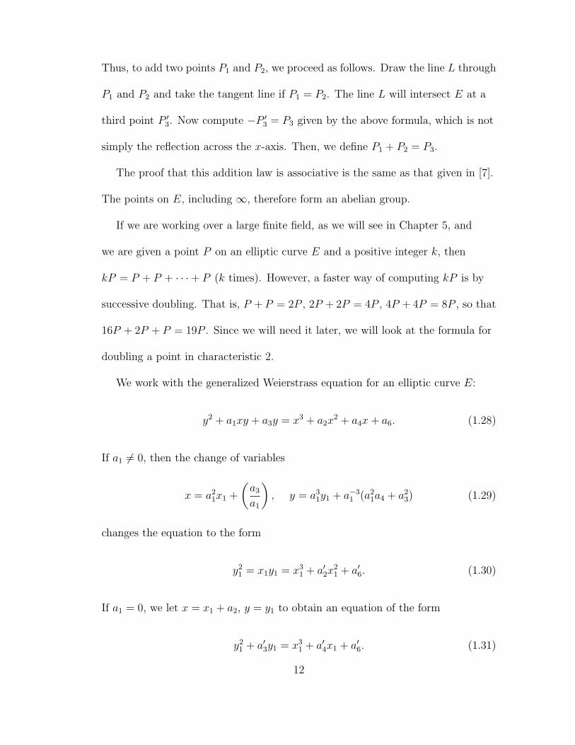
Thus, to add two points P1 and P2, we proceed as follows. Draw the line L through

P1 and P2 and take the tangent line if P1 = P2. The line L will intersect E at a

third point P ′3. Now compute −P ′3 = P3 given by the above formula, which is not

simply the reflection across the x-axis. Then, we define P1 + P2 = P3.

The proof that this addition law is associative is the same as that given in [7].

The points on E, including ∞, therefore form an abelian group.

If we are working over a large finite field, as we will see in Chapter 5, and

we are given a point P on an elliptic curve E and a positive integer k, then

kP = P + P + · · ·+ P (k times). However, a faster way of computing kP is by

successive doubling. That is, P + P = 2P , 2P + 2P = 4P , 4P + 4P = 8P , so that

16P + 2P + P = 19P . Since we will need it later, we will look at the formula for

doubling a point in characteristic 2.

We work with the generalized Weierstrass equation for an elliptic curve E:

y2 + a1xy + a3y = x3 + a2x2 + a4x+ a6. (1.28)

If a1 6= 0, then the change of variables

x = a21x1 +

(a3

a1

), y = a3

1y1 + a−31 (a2

1a4 + a23) (1.29)

changes the equation to the form

y21 = x1y1 = x3

1 + a′2x21 + a′6. (1.30)

If a1 = 0, we let x = x1 + a2, y = y1 to obtain an equation of the form

y21 + a′3y1 = x3

1 + a′4x1 + a′6. (1.31)

12

The first case will be for curves of the form, y2 + xy = x3 + a2x2 + a6. An

equation of this form is equivalent to y2 + xy + x3 + a2x2 + a6 = 0, since we are

performing operations in characteristic 2. Thus, by implicit differentiation

2ydy

dx+ x

dy

dx+ y + 3x2 + 2a2x = x

dy

dx+ y + x2 = 0 =⇒ dy

dx=x2 + y

x, (1.32)

we see that the slope of L through P = (x0, y0) is

m =dy

dx=y0 + x2

0

x0

. (1.33)

Thus, the equation of L is y = m(x− x0) + y0 = mx+ b for some b, so by

substitution we find

x1 = m2 +m+ a2 =y2

0 + x40 + x0y0 + x3

0 + a2x20

x20

=x4

0 + a6

x20

(1.34)

since y20 = x0y0 +x3

0 +a2x20 +a6 and y1 = m(x−x0)+y0. The point (x1, y1) = −2P

so that (x2, y2) = 2P with

x2 =x4

0 + a6

x20

, y2 = −x1 − y1 = x1 + y1. (1.35)

For curves of the other form, y2 + a3y = x3 + a4x+ a6, we rewrite this as

y2 + a3y + x3 + a4x+ a6 = 0. Therefore, by a similar argument as in the previous

case we find that 2P = (x2, y2) where

x2 =x4

0 + a24

a23

, y2 = a3 + y1. (1.36)

1.5 Endomorphisms

The main purpose of this section is to prove Proposition 1.5.1, which will be

used in the proof of Hasse’s theorem. By an endomorphism of an elliptic curve E,

13

we mean a group homomorphism α : E(K) −→ E(K) that is given by rational

functions. In other words, α(P1 + P2) = α(P1) + α(P2), and there are rational

functionsR1(x, y), R2(x, y) with coefficients inK with α(x, y) = (R1(x, y), R2(x, y))

for all (x, y) ∈ E(K). Since α is a homomorphism, we have α(∞) =∞.

It is useful to have a standard form for the rational functions describing an

endomorphism. We assume that an elliptic curve E is given in Weierstrauss form.

Let R(x, y) be any rational function. Since y2 = x3 + ax+ b for all (x, y) ∈ E(K),

we can replace any even power of y by a polynomial in x and obtain a rational

function that gives the same function as R(x, y) on points of E(K). Therefore, we

may assume

R(x, y) =p1(x) + p2(x)y

p3(x) + p4(x)y. (1.37)

Thus, by rationalization and replacing y2 with x3 + ax+ b we obtain

R(x, y) =q1(x) + q2(x)y

q3(x). (1.38)

Now consider an endomorphism given by α(x, y) = (R1(x, y), R2(x, y)) as before.

Since α is a homomorphism, α(x,−y) = −α(x, y) so that R1(x,−y) = R1(x, y)

and R2(x,−y) = −R2(x, y). Therefore, if R1(x, y) is in the form (1.38), then

q2(x) = 0 and if R2(x, y) is in the form (1.38), then q1(x) = 0. Thus, we may

assume that α(x, y) = (r1(x), r2(x)y) with rational functions r1(x) and r2(x).

We can now discuss what happens when a rational function is not defined at

a point. Write

r1(x) =p(x)

q(x)(1.39)

be such that gcd(p(x), q(x)) = 1. If q(x) = 0 for some point (x, y), then we assume

14

that α(x, y) =∞. If q(x) 6= 0, then r2(x) is defined and thus the rational functions

defining α are defined.

We define the degree of an endomorphism α to be

deg(α) = max {deg(p(x)), deg(q(x))} (1.40)

provided that α is nontrivial, that is, an endomorphism that does not send all

points (x, y) to ∞. When α = 0, let deg(0) = 0. Define α 6= 0 to be a separable

endomorphism if the derivative r′1(x) is not identically zero. Note that this is

equivalent to saying that at least one of p′(x) and q′(x) is not identically zero.

We are now ready to state Proposition 1.5.1 which will be crucial in the proof

of Hasse’s theorem.

Proposition 1.5.1. Let α 6= 0 be a separable endomorphism of an elliptic

curve E. Then

deg(α) = #Ker(α), (1.41)

where Ker(α) is the kernel of the homomorphism α : E(K) −→ E(K). If α 6= 0

is not separable, then

deg(α) > #Ker(α). (1.42)

Proof. Write α(x, y) = (r1(x), r2(x)y) with r1 and r2 as above. Then r′1(x) 6= 0, so

p′(x)q(x)− p(x)q′(x) 6= 0. Let S ={x ∈ K | (p′(x)q(x)− p(x)q′(x))q(x) = 0

}.

Let (a, b) ∈ E(K) be such that

(1) a 6= 0, b 6= 0, and (a, b) 6=∞,

(2) deg(p(x)− aq(x)) = max {deg(p(x)), deg(q(x))} = deg(α),

15

(3) a /∈ r1(S), and

(4) (a, b) ∈ α(E(K)).

Since p′(x)q(x)− p(x)q′(x) 6= 0, we have S is a finite set and hence α(S) is finite as

well. The function r1(x) takes on infinitely many distinct values as x runs through

K. Since, for each x, there is a point (x, y) ∈ E(K), we see that α(E(K)) is an

infinite set. Therefore, such a point (a, b) exists.

We claim that there are exactly deg(α) points (x1, y1) ∈ E(K) such that

α(x1, y1) = (a, b). For such a point, we have

p(x1)

q(x1)= a, r2(x1)y1 = b. (1.43)

Since (a, b) 6=∞, we must have q(x1) 6= 0 so r2(x1) is defined. Since b 6= 0 and

r2(x1)y1 = b, we must have y1 = b/r2(x1). Therefore, x1 determines y1 in this case,

so we only need to count values of x1.

By assumption (2), p(x)− aq(x) = 0 has deg(α) roots, counting multiplicities.

We therefore must show that p(x)− aq(x) has no multiple roots. Suppose that x0

is a multiple root. Then p(x0)− aq(x0) = 0 and p′(x0)− aq′(x0) = 0. Multiplying

the equations p(x) = aq(x) and aq′(x) = p′(x) yields ap(x0)q′(x0) = ap′(x0)q(x0).

Since a 6= 0, this implies that x0 is a root of p(x)q′(x)− p′(x)q(x), so x0 ∈ S.

Therefore, a = r1(x0) ∈ r1(S), contrary to assumption. It follows that p(x)−aq(x)

has no multiple roots, and therefore has deg(α) distinct roots.

Since there are exactly deg(α) points (x1, y1) with α(x1, y1) = (a, b), we see

that #Ker(α) = deg(α). Furthermore, if α is not separable, then the steps of the

proof hold, except that p′(x)− aq′(x) = 0, so p(x)− aq(x) = 0 always has multiple

16

roots and therefore has fewer than deg(α) solutions.

One important example of an endomorphism is the Frobenius map, which

plays a crucial role in the theory of elliptic curves over Fq. Suppose that E is

an elliptic curve defined over a finite field Fq. The Frobenius map is defined as

ϕq(x, y) = (xq, yq). Note that if E is an elliptic curve defined over a finite field Fq,

then ϕq is an endomorphism of degree q and is not separable.

1.6 Singular Curves

We have been working with y2 = x3 + ax+ b under the assumption that

x3 + ax+ b has distinct roots. However, when there are multiple roots it turns

out that elliptic curve addition becomes either addition of elements in K or

multiplication of elements in K× or in a quadratic extension of K. This means

that an algorithm for a group E(K) arising from elliptic curves, such as the

discrete logarithm problem, will probably also apply to these more familiar

situations. Moreover, we will also see that singular curves arise naturally when

elliptic curves defined over the integers are reduced modulo various primes.

First consider the case where x3 + ax+ b has a triple root at x = 0, so the

curve becomes y2 = x3. Note that only (0, 0) is a singular point on the curve, since

any line through (0, 0) intersects the curve at most one other point. Therefore,

we exlude the point (0, 0) from the group so that addition may be defined on the

curve. The set of all remaining form a group with the same group law as in the

case when the cubic has distinct roots. We need to check that addition of any two

points on the cubic does not yield the excluded point (0, 0). However, a line through

17

two nonsingular points cannot pass through (0, 0), so this is not a problem.

The next theorem is Theorem 2.30 in [7] and shows that whenever the cubic has

a triple root, or cusp, the group of nonsingular points on the curve, with

coordinates considered in K, is isomorphic to K.

Theorem 1.6.1. Let E be the curve y2 = x3 and let Ens(K) be the nonsingular

points on this curve, regarded as an additive group, with coordinates in K including

the point ∞ = (0 : 1 : 0). The map

ϕ : Ens(K) −→ K (1.44)

given by (x, y) 7→ x/y and ∞ 7→ 0 is a group isomorphism.

Now we consider the second case where x3 + ax+ b has a double root. By

translation we may regard the double root at x = 0 so that the curve becomes

y2 = x2(x+ a) (1.45)

for some a 6= 0. The only singular point is (0, 0) for the same reason as above.

Again, consider the group of all nonsingular points of the curve with coordinates

in K including ∞. Let α2 = a, so that α might lie in an extension of K.

The equation (1.45) may be written as

(yx

)2

= x+ a. (1.46)

Note that whenever x→ 0, then the right-hand side of (1.46) is approximately a.

Therefore, the curve is approximated by tangent lines y = αx and y = −αx near

x = 0 and we obtain the next theorem, which is Theorem 2.31 in [7].

18

Theorem 1.6.2. Let E be the curve y2 = x2(x+ a), where a ∈ K×. Let Ens(K)

be the nonsingular points on E with coordinates in K.

Let α2 = a and consider the map

ϕ : (x, y) 7→ y + αx

y − αx, and ∞ 7→ 1. (1.47)

(1) If α ∈ K then Ens(K) ∼= K×, considered a multiplitative group.

(2) If α /∈ K then Ens(K) ∼= {u+ αv | u, v ∈ K, u2 − av2 = 1}, considered a

group under multiplication.

One situation that arises when we consider singular curves is when we consider

curves with integral coefficients and reduce modulo various prime numbers.

Example 1.6.3. Let E be the elliptic curve y2 = x(x+ 35)(x− 55), then we have

the following situations.

E (mod 5) : y2 ≡ x3 (1.48)

E (mod 7) : y2 ≡ x2(x− 6) ≡ x2(x+ 1) (1.49)

E (mod 11) : y2 ≡ x2(x+ 2) (1.50)

The case (1.48) is exactly in the form of Theorem 1.6.1, which implies that

Ens(F5) ∼= F5 and is called an additive reduction. The second case (1.49) is called

a split multiplicative reduction and is covered by Theorem 1.6.2(1) and states

that Ens(F7) ∼= F×7 . Finally, (1.50) is in the form of Theorem 1.6.2(2) since

α = 22 = 4 /∈ F11 and is called a nonsplit multiplication reduction.

19

Chapter 2

Torsion Points

The torsion points, namely those that have finite order, play an important role in

the study of elliptic curves. In Chapter 3, we will see that all points are torsion

points on an elliptic curve over a finite field. We then study the properties of the

Weil pairing, which is used in the proof of Hasse’s theorem and in Chapter 4 to

attack the elliptic curve discrete logarithm problem.

2.1 Torsion Points

We begin by defining the set of all torsion points of order n.

Defintion 2.1.1. Let E be an elliptic curve defined over a field K. Let n be a

positive integer, then the set of n-torsion points is

E[n] ={P ∈ E(K) | nP =∞

}. (2.1)

Note that the set E[n] contains points with coordinates in K, not just in K.

Whenever char(K) 6= 2, then we can describe the set E[2]. Let

y2 = (x− e1)(x− e2)(x− e3) (2.2)

with e1, e2, e3 ∈ K. Recall from Theorem 1.2.1 that 2P =∞ if and only if the

20

tangent line at P is vertical. Therefore, we see that y = 0 and thus

E[2] = {∞, (e1, 0), (e2, 0), (e3, 0)} ∼= Z2 ⊕ Z2. (2.3)

However, when char(K) = 2 we have seen that E has the form

y2 + xy + x3 + a2x2 + a6 = 0 (2.4)

or the form

y2 + a3y + x3 + a4x+ a6 = 0. (2.5)

To avoid the case where the curve becomes singular, (2.4) must have that a6 6= 0

and (2.5) must have a3 6= 0. If P = (x, y) is point of order 2, then the tangent line

at P is vertical. This means that d/dy(x, y) = 0. In (2.4), this means that x = 0

so by substitution we see that

y2 + xy + x3 + a2x2 + a6 = y2 + a6 = 0 =⇒ (y +

√a6)

2= 0. (2.6)

Therefore, (0,√a6) is the only point of order 2, so that E[2] =

{∞, (0,√a6)

} ∼= Z2.

In addition, we see that whenever d/dy(x, y) = a3 6= 0 there is no point of

order 2 for elliptic curves of the form (2.5). In this case, E[2] = {∞}.

Proposition 2.1.2. Let E be an elliptic curve over a field K. If char(K) 6= 2,

then E[2] ∼= Z2 ⊕ Z2. If char(K) = 2, then E[2] ∼= 0 or E[2] ∼= Z2.

Now we consider the set E[3]. Again we assume that char(K) 6= 2, 3, then we

can represent E by (1.1). A point P satisfies 3P =∞ if and only if 2P = −P .

Thus, the x-coordinate of 2P is the x-coordinate of P , but the y-coordinates of the

two points differ by a sign. If the y-coordinates were the same, then 2P = P would

imply that that P =∞.

21

Using the formulas derived in Theorem 1.2.1, we see that

x = m2 − 2x and y =3x2 + a

2m. (2.7)

Therefore, y2 = x3 + ax+ b becomes(3x2 + a

2m

)2

= x3 + ax+ b =⇒ 3x4 + 6ax2 + 12bx− a2 = 0. (2.8)

The discriminant of this polynomial is ∆ = −6912(4a3 + 27b2)2 6= 0. Hence,

the polynomial has no multiple roots, so that there are four distinct values of x.

Further, each value of x gives two different values of y. So we have 8 points of

order 3 together with ∞. Thus, E[3] ∼= Z3 ⊕ Z3.

Whenever the char(K) = 2, we use a similar argument with the formulas given

in (1.35) and (1.36). If char(K) = 3 then we may assume that E has the form

y2 = x3 + a2x2 + a4x+ a6. (2.9)

Again we have that 2P = −P implies that the x-coordinates of the two points

are the same. Since char(K) = 3 we obtain(2a2x+ a4

2y

)2

− a2 = 3x = 0. (2.10)

However, (2.10) implies that a2x3 + a2a6 − a2

4 = 0 since 4 ≡ 1 (mod 3). Note that

we cannot have that a2 = a4 = 0, since that would imply x3 + a6 = (x+ 3√a6)

3 has

multiple roots. Thus, at least one of a2 or a4 is nonzero.

If a2 = 0, then we have that −a24 = 0 which cannot occur. Thus, there are no

values of x and E[3] = {∞}. On the other hand, if a2 6= 0 then a2(x3 + a) = 0

which gives a triple root in characteristic 3. Thus, there is one x-value and two

corresponding y-values. This gives two points of order 3 and∞, so that E[3] ∼= Z3.

22

The general situation is given as the following, which is Theorem 3.2 in [7].

Theorem 2.1.3. Let E be an elliptic curve over a field K and let n be a positive

integer. If char(K) - n or char(K) = 0, then

E[n] ∼= Zn ⊕ Zn. (2.11)

If char(K) = p > 0 and p|n, we write n = prn′ where p - n′, then

E[n] ∼= Zn′ ⊕ Zn′ or E[n] ∼= Zn ⊕ Zn′ . (2.12)

In the case where an elliptic curve E is defined over a field K such that

char(K) = p, then E is called ordinary if E[p] ∼= Zp. If E[p] ∼= 0, then E is called

supersingular. This is not to be confused with singular curves, which are curves

that contain at least one singular point.

Now let n be a positive integer such that char(K) - n. Choose a basis {β1, β2}

for E[n] ∼= Zn ⊕ Zn. Then every element of E[n] can be expressed as a linear

combination of β1 and β2. Note that the coefficients are uniquely determined

modulo n.

Let αn : E(K) −→ E(K) be a group homomorphism, then α maps E[n] into

E[n] by restriction. Thus, there exists a, b, c, d ∈ Zn such that α(β1) = aβ1 + cβ2

and α(β2) = bβ1 + dβ2. Thus, each homomorphism α : E(K) −→ E(K) is

represented by a 2× 2 matrix

αn =

[a bc d

]. (2.13)

Composition of group homomorphisms corresponds to multiplication of matrices.

23

2.2 The Weil Pairing

We now discuss the Weil pairing on the n-torsion of an elliptic curve. Let E be

an elliptic curve over a field K and n be an integer such that char(K) - n. Then,

Theorem 2.1.3 states that E[n] ∼= Zn ⊕ Zn.

Let µn ={x ∈ K | xn = 1

}be the group of nth roots of unity in K. Since

char(K) - n, the equation xn = 1 has no multiple roots, thus has n distinct roots

in K. Therefore, µn is a cyclic group of order n. Any generator ζ of µn is called a

primitive nth root of unity.

The following theorem is Theorem 3.9 in [7], which defines the Weil pairing and

properties that the pairing must satisfy.

Theorem 2.2.1. Let E be an elliptic curve defined over a field K and let n be a

positive integer such that char(K) - n. Then there is a pairing

en : E[n]× E[n] −→ µn, (2.14)

called the Weil pairing that satisfies the following properties:

(1) en is bilinear in each variable. In other words,

en(P1 + P2, Q) = en(P1, Q)en(P2, Q) (2.15)

and

en(P,Q1 +Q2) = en(P,Q1)en(P,Q2) (2.16)

for all P, P1, P2, Q,Q1, Q2 ∈ E[n].

(2) en is nondegenerate in each variable. This means that if en(P,Q) = 1 for

all Q ∈ E[n], then P =∞ and similarly if en(P,Q) = 1 for all P ∈ E[n],

24

then Q =∞.

(3) en(P, P ) = 1, for all P ∈ E[n].

(4) en(P,Q) = en(Q,P )−1 for all P,Q ∈ E[n].

(5) en(σP, σQ) = σ(en(P,Q)) for all automorphisms σ of K such that σ is the

identity map on the coefficients of E.

(6) en(α(P ), α(Q)) = en(P,Q)deg(α) for all separable endomorphisms α of E.

If the coefficients of E lie in a finite field Fq, then the statement also holds

when α is the Frobenius endomorphism ϕq.

Corollary 2.2.2. Let {P1, P2} be a basis of E[n], then en(P1, P2) is a primitive

nth root of unity.

Proof. Suppose that en(P1, P2) = ζ with ζd = 1, then en(P1, dP2) = 1. In addition,

en(P2, dP2) = en(P2, P2)d = 1 by Theorem 2.2.1(1) and (3).

Let P ∈ E[n] then P = aP1 + bP2 for some a, b ∈ Z. Hence,

en(P, dP2) = en(aP1 + bP2, dP2) = en(P1, dP2)aen(P2, dP2)

b = 1. (2.17)

Since (2.17) holds for all P ∈ E[n], then Theorem 2.2.1(2) implies that dP2 =∞.

Since dP2 =∞ if and only if n|d, we find that ζ is a primitive nth root of unity.

We now use the Weil pairing to deduce two statements that will be used in the

proof of Hasse’s theorem in Chapter 3. Recall that α is an endomorphism of E,

then we obtain a matrix of the form (2.13) with entries in Zn, describing the group

action α on a basis {P1, P2}.

Proposition 2.2.3. Let α be an endomorphism of an elliptic curve E defined

25

over a field K. Let n be a positive integer such that char(K) - n. Then

deg(αn) ≡ deg(α) (mod n).

Proof. Suppose that ζ = en(P1, P2) be a primitive nth root of unity. By Theorem

2.2.1(6), we see that

ζdeg(α) = en(α(P1), α(P2)) = en(aP1 + cP2, bP1 + dP2)

= en(P1, P1)aben(P1, P2)

aden(P2, P1)bcen(P2, P2)

cd

= en(P1, P2)aden(P1, P2)

−bc = en(P1, P2)ad−bc = ζad−bc, (2.18)

by the properties of the Weil pairing. Since ζ is a primitive nth root of unity,

deg(α) ≡ (ad− bc) (mod n).

The previous result allows us to reduce questions about the degree of an

endomorphism to calculations with matrices. Now let α and β be endomorphisms

of E and a, b ∈ Z. If we let P = (x, y) be a point on E, then the endomorphism

aα + bβ is defined by

(aα + bβ)(x, y) = aα(x, y) + bβ(x, y). (2.19)

Here aα(x, y) means multiplication on E of α(x, y) by a. Similiarly for bβ(x, y),

then the results are added on E. This process can all be described by rational

functions since this is true for each of the individual steps. Therefore, aα + bβ

is an endomorphism.

Proposition 2.2.4. Let a, b ∈ Z. Then for any endomorphisms α and β

deg(aα+ bβ) = a2 deg(α) + b2 deg(β) + ab(deg(α+ β)− deg(α)− deg(β)). (2.20)

26

Proof. Let n be a positive integer such that char(K) - n. Represent α and β by

matrices αn and βn with respect to some basis of E[n]. Then aαn + bβn gives the

action of aαn + bβn on E[n]. Therefore, we have that

det (aαn + bβn)) =

a2 det(αn) + b2 det(βn) + ab(det(αn + βn)− det(αn)− det(βn))

(2.21)

for any matrices αn and βn. Hence,

deg(aα + bβ) ≡

(a2 deg(α) + b2 deg(β) + ab(deg(α + β)− deg(α)− deg(β))) (mod n).

(2.22)

Since (2.22) holds for infinitely many n, we obtain (2.20).

27

Chapter 3

Elliptic Curves over Finite Fields

Whenever E is an elliptic curve over a finite field K, then there are only finitely

many points (x, y) with x, y ∈ K. Therefore, the additive group E(K) is finite

and so can we can apply theorems from finite group theory. The main result in

this chapter is Hasse’s theorem, which is proved in Section 3.2, and allows us to

provide a bound on the order of E(K). We conclude this chapter with applications

of Hasse’s theorem to find the order of points on E and ultimately methods to

calculate the order of E(K).

3.1 Introduction

We begin with some examples of elliptic curves over various finite fields. All

the results from Chapter 1 still hold, however, all calculations are performed over

a finite field K.

Example 3.1.1. Let E be an elliptic curve defined by y2 = x3 + x+ 1 over F5.

One way to determine the order of E(F5) is to list all possible values of x ∈ F5,

then calculate x3 + x+ 1 (mod 5). Finally, we find the square roots of x3 + x+ 1

over F5, which gives points on E(F5) as shown in Table 3.1.

28

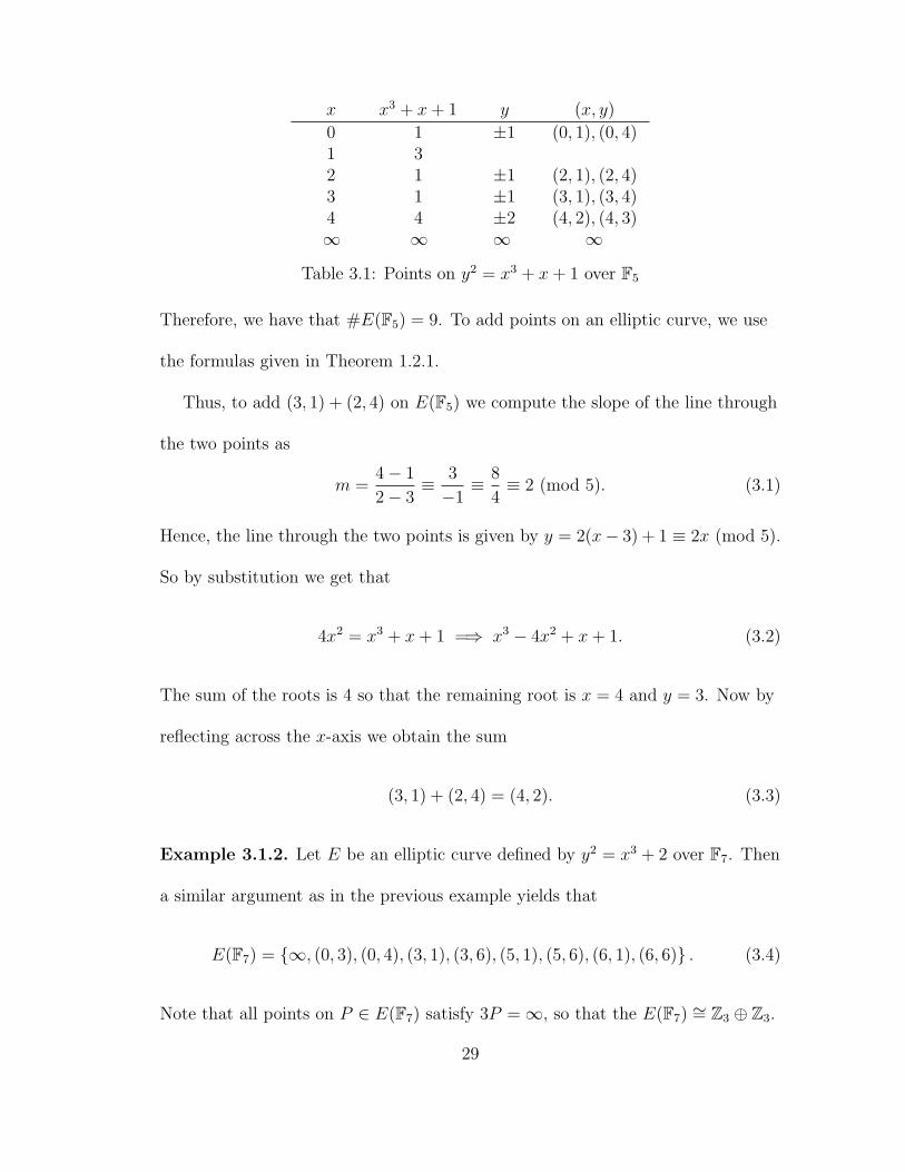
x x3 + x+ 1 y (x, y)

0 1 ±1 (0, 1), (0, 4)1 32 1 ±1 (2, 1), (2, 4)3 1 ±1 (3, 1), (3, 4)4 4 ±2 (4, 2), (4, 3)∞ ∞ ∞ ∞

Table 3.1: Points on y2 = x3 + x+ 1 over F5

Therefore, we have that #E(F5) = 9. To add points on an elliptic curve, we use

the formulas given in Theorem 1.2.1.

Thus, to add (3, 1) + (2, 4) on E(F5) we compute the slope of the line through

the two points as

m =4− 1

2− 3≡ 3

−1≡ 8

4≡ 2 (mod 5). (3.1)

Hence, the line through the two points is given by y = 2(x− 3) + 1 ≡ 2x (mod 5).

So by substitution we get that

4x2 = x3 + x+ 1 =⇒ x3 − 4x2 + x+ 1. (3.2)

The sum of the roots is 4 so that the remaining root is x = 4 and y = 3. Now by

reflecting across the x-axis we obtain the sum

(3, 1) + (2, 4) = (4, 2). (3.3)

Example 3.1.2. Let E be an elliptic curve defined by y2 = x3 + 2 over F7. Then

a similar argument as in the previous example yields that

E(F7) = {∞, (0, 3), (0, 4), (3, 1), (3, 6), (5, 1), (5, 6), (6, 1), (6, 6)} . (3.4)

Note that all points on P ∈ E(F7) satisfy 3P =∞, so that the E(F7) ∼= Z3 ⊕ Z3.

29

Two main restrictions on the groups E(Fq) are given in the next two results.

Theorem 3.1.3. Let E be an elliptic curve over the finite field E(Fq), then

E(Fq) ∼= Zn (3.5)

for some n ≥ 1, or

E(Fq) ∼= Zn1 ⊕ Zn2 (3.6)

for some integers n1, n2 ≥ 1 such that n1|n2.

Proof. Recall from group theory that a finite abelian group is isomorphic to a direct

sum of cyclic groups

Zn1 ⊕ Zn2 ⊕ · · ·Znr , (3.7)

with ni|ni+1 for i ≥ 1. Since, for each i, the group Znihas n1 elements of order

dividing n1, we find that E(Fq) has nr1 elements of order dividing n1. Thus, by

Theorem 2.1.3, there are at most n21 such points. Therefore, r ≤ 2 and we obtain

the result.

Theorem 3.1.4 (Hasse). Let E be an elliptic curve over a finite field Fq, then

|q + 1−#E(Fq)| ≤ 2√q. (3.8)

The theorem will be proved in Section 3.2. Now we turn our attention to the groups

that can actually occur as groups E(Fq). The answer is given in the following two

results, which are proved in [2] and [8], respectively.

Theorem 3.1.5. Let q = pn be a power of a prime number p and let N = q+1−a.

There is an elliptic curve E defined over Fq such that #E(Fq) = N if and only if

|a| ≤ 2√q and a satisfies one of the following:

30

(1) gcd(a, p) = 1

(2) n is even and a = ±2√q

(3) n is even, p 6≡ 1 (mod 3), and a = ±√q

(4) n is odd, p = 2 or p = 3, and a = ±p(n+1)/2

(5) n is even, p 6≡ 1 (mod 4), and a = 0

(6) n is odd and a = 0.

Theorem 3.1.6. Let N be an integer that occurs as the order of an elliptic curve

over a finite field Fq, as in Theorem 3.1.5. Write N = pen1n2 with p - n1n2 and

n1|n2. There is an elliptic curve E over Fq such that

E(Fq) ∼= Zpe ⊕ Zn1 ⊕ Zn2 (3.9)

if and only if

(1) n1|(q − 1) in (1), (3), (4), (5), and (6) of Theorem 3.1.5.

(2) n1 = n2 in (2) of Theorem 3.1.5.

These are the only groups that occur as groups E(Fq).

3.2 The Frobenius Endorphism

Let Fq be a finite field with algebraic closure Fq and let

ϕq : Fq −→ Fq (3.10)

given by x 7→ xq be the Frobenius map for Fq.

Let E be an elliptic curve defined over Fq, then ϕq acts on the coordinates of

points in E(Fq) by ϕq(x, y) = (xq, yq) and ϕq(∞) =∞.

31

Lemma 3.2.1. Let E be defined over Fq and let (x, y) ∈ E(Fq).

(1) ϕq(x, y) = (xq, yq) ∈ E(Fq)

(2) (x, y) ∈ E(Fq) if and only if ϕq(x, y) = (x, y)

Proof. Since the proofs are the same for the Weierstrauss and the generalized

Weierstrauss equations, we work with the general form. We have

y2 + a1xy + a3y = x3 + a2x2 + a4x+ a6 (3.11)

with a1, a2, a3, a4, a6 ∈ Fq. Now by raising each to the qth power to obtain

(yq)2 + a1(xqyq) + a3(y

q) = (xq)3 + a2(xq)2 + a4(x

q) + a6. (3.12)

Note this shows that (xq, yq) ∈ E(Fq).

To show (2), recall that x ∈ Fq if and only if ϕq(x) = x and similarly for y ∈ Fq.

Therefore, we find that

(x, y) ∈ E(Fq)⇐⇒ x, y ∈ Fq ⇐⇒ ϕq(x) = x and ϕq(y) = y

⇐⇒ ϕq(x, y) = (x, y).

(3.13)

Hence, we have shown (1) and (2), so we obtain the result.

The following result is crucial to counting points on an elliptic curve over

finite fields. Since ϕq is an endomorphism, then so it ϕnq = ϕq ◦ ϕq ◦ · · · ◦ ϕq

for every n ≥ 1. Since multiplication by (−1) is also an endorphism, then ϕnq − 1

is an endorphism of E.

Proposition 3.2.2. Let E be defined over Fq and let n ≥ 1, then

(1) Ker(ϕnq − 1) = E(Fqn)

(2) ϕnq − 1 is a separable endomorphism, so #E(Fqn) = deg(ϕnq − 1).

32

Proof. Since ϕnq is the Frobenius map for hte field Fqn , then (1) is a restatement

of Lemma 3.2.1. The fact that ϕnq is separable is due to q - (−1). Therefore, (2)

follows from Proposition 1.5.1.

We need one more result before we are ready to prove Hasse’s theorem.

In preparation for the next result, let

a = q + 1−#E(Fq) = q − 1− deg(ϕq − 1). (3.14)

Lemma 3.2.3. Let r, s ∈ Z with gcd(s, q) = 1, then deg(rϕq− s) = r2q+ s2− rsa.

Proof. Note that Proposition 2.2.4 and (3.14) implies that

deg(rϕq − s) = r2 deg(ϕq) + s2 deg(−1) + rs((deg(ϕq − 1))− deg(ϕ)− deg(−1))

= r2q + s2 + rs(deg(ϕq − 1)− q − 1)

= r2q + s2 + rs(deg((q + 1− a)− q − 1)) (3.15)

= r2q + s2 + rsa.

Note that we did not need the assumption that gcd(s, q) = 1.

Proof of Theorem 3.1.4. We want to show from (3.14) that |a| ≤ 2√q. Since

deg(rϕq − s) ≥ 0, Lemma 4.2.3 implies that

r2q + s2 − rsa =qr2

s2− rsa

s2+ 1 = q

(rs

)2

− a(rs

)+ 1 ≥ 0 (3.16)

for all r, s ∈ Z with gcd(s, q) = 1. The set

{rs| gcd(s, q) = 1

}⊂ Q (3.17)

33

is dense in R. Therefore, qx2 − ax+ 1 ≥ 0, for all x ∈ R and the discriminant is

negative or zero, which means that

a2 − 4q ≤ 0 =⇒ |a| ≤ 2√q. (3.18)

This proves Hasse’s theorem and gives bounds for the group of points on an elliptic

curve over a finite field.

3.3 Applications of Hasse’s Theorem

Now that we have established Hasse’s theorem, we have only found bounds for

the order of the group of points on an elliptic curve over a finite field. In this

section we provide three methods for actually determining the order of the group.

Suppose that we have an elliptic curve E defined over a finite field Fq and we

want to know #E(Fqn) for some n. We can determine #E(Fqn) when n = 1 by

listing the elements, which allows us to determine #E(Fqn) for some n as the

following theorem illustrates.

Theorem 3.3.1. Let #E(Fq) = q + 1− a. Write x2 − ax+ q = (x− α)(x− β),

then

#E(Fqn) = qn + 1− (αn + βn) (3.19)

for all n ≥ 1.

Proof. First, recall that αn + βn is an algebraic integer and a rational number,

34

so that αn + βn is an integer. Now let

f(x) = (xn − αn)(xn − βn) = x2n − (αx)n − (βx)n + (αβ)n

= x2n − (αn + βn)x+ (αβ)n

= x2n − (αn + βn)x+ qn.

(3.20)

Then, x2 − ax+ q = (x− α)(x− β)|f(x). Therefore, it follows from the division

algorithm that the quotient g(x) ∈ Z[x]. Thus,

(ϕnq )2 − (αn + βn)ϕnq + qn = f(ϕq) = g(ϕq)(ϕ2q − aϕq + q) = 0 (3.21)

as endorphisms of E. Note that ϕnq = ϕqn , so there is only one integer k such that

ϕ2qn − kϕqn + qn = 0 and such k is determined by k = qn + 1−#E(Fqn). Thus,

αn + βn = qn + 1−#E(Fqn). (3.22)

This completes the proof of Theorem 3.3.1.

In the previous section, to make a list of points on y2 = x3 + ax+ b over a finite

field, we tried each possible value of x, then found the square roots y of x3 +ax+ b

if they existed. This method is the foundation for a simple point counting

algorithm.

Recall the Legendre symbol(xp

)for an odd prime p is defined as follows:

(x

p

)=

+1 if t2 ≡ x (mod p) has a solution t 6≡ 0 (mod p),−1 if t2 ≡ x (mod p) has no solution t,

0 if x ≡ 0 (mod p).(3.23)

This idea can be generalized to any finite field Fq with q an odd prime by defining

35

for x ∈ Fq, (x

Fq

)=

+1 if t2 = x has a solution t ∈ F×q ,−1 if t2 = x has no solution t ∈ Fq,

0 if x = 0.(3.24)

Theorem 3.3.2. Let E be an elliptic curve defined by y2 = x3 + ax+ b over Fq,

then we have that

#E(Fq) = q + 1 +∑x∈Fq

(x3 + ax+ b

Fq

). (3.25)

Proof. For a given x0 there are two points (x, y) with x-coordinate x0 if x30 +ax0 +b

is a nonzero square in Fq, one point if it is zero, and no points if it is not a square.

Therefore, the number of points with x-coordinate x0 equals 1 +(x30+ax0+b

Fq

).

Summing over all x0 ∈ Fq and including 1 for the point ∞ gives

#E(Fq) = 1 +∑x∈Fq

(1 +

(x3 + ax+ b

Fq

))= q + 1 +

∑x∈Fq

(x3 + ax+ b

Fq

). (3.26)

This completes the proof of Theorem 3.3.2.

Example 3.3.3. Let E be the elliptic curve defined by y2 = x3 + x + 1 over F5.

The nonzero squares modulo 5 are 1 and 4. Therefore,

#E(F5) = 5 + 1 +∑x∈F5

(x3 + x+ 1

F5

)= 5 + 1 +

4∑x=0

(x3 + x+ 1

5

)= 6 +

(1

5

)+

(3

5

)+

(11

5

)+

(31

5

)+

(69

5

)= 6 +

(1

5

)+

(3

5

)+

(1

5

)+

(1

5

)+

(4

5

)= 6 + 1− 1 + 1 + 1 + 1 = 9.

(3.27)

Theorem 3.3.2 is sometimes referred to as the Lang-Trotter method, which works

quickly for small values of q, that is for q < 100, but is slow for larger values of q

and is impossible to use when q is around 10100 or larger.

36

Another useful technique to find the order of the group is to determine the order

of points on an elliptic curve along with Hasse’s theorem to narrow the search for

the order of the group. Thus, let P ∈ E(Fq) then the order of P is the smallest

positive integer k such that kP =∞. By Lagrange’s theorem, the order of P

always divides the order of the group E(Fq). Furthermore, recall that if nP =∞

for n ∈ Z if and only if the order of P divides n.

By Hasse’s theorem, the order of E(Fq) lies in an interval of length 4√q.

Therefore, if we find that a point that has order greater than 4√q, then there

can only be one multiple of the order of the point smaller than 4√q and must be

#E(Fq). In addition, using a few more points often shortens the list enough that

there is a unique possibility for #E(Fq).

Example 3.3.4. Let E be the elliptic curve y2 = x3 + 7x+ 12 over F103. It is

possible to see that (−1, 2) has order 13 and the point (19, 0) has order 2, so that

N103 = #E(F103) is a multiple of 26. Hasse’s theorem implies that

103 + 1− 2√

103 ≤ N103 ≤ 103 + 1 + 2√

103 =⇒ 84 ≤ N103 ≤ 124. (3.28)

The only multiple of 26 in this interval is 104, so N103 = #E(F103) = 104.

Example 3.3.5. Let E be the elliptic curve y2 = x3 + 2 over F7 as in Example

4.1.2. We have already observed that E(F7) ∼= Z3 ⊕ Z3, since every point except

∞ has order 3. Thus, we can only conclude that N7 = #E(F7) is a multiple of 3

and by Hasse’s theorem get that 3 ≤ N7 ≤ 13. This leaves 3, 6, 9, and 12

as possibilities.

If we can find two points of order 3 that are not multiples of one another, then

37

they generate a subgroup of order 9. This means that the order of the group is a

multiple of 9, so that N7 = 9.

The situation where E(Fq) ∼= Zn⊕Zn as in the previous example makes it more

difficult to find #E(Fq), but due to the next result, this situation is rare.

Proposition 3.3.6. Let E be an elliptic curve over Fq and suppose that

E(Fq) ∼= Zn ⊕ Zn (3.29)

for some n ∈ Z. Then either q = n2 + 1 or q = n2 ± n+ 1, or q = (n± 1)2.

Proof. By Hasse’s theorem, n2 = q + 1− a with |a| ≤ 2√q. Thus to prove the

statement, we need the following lemma that places a restriction on a.

Lemma 3.3.7. a ≡ 2 (mod n).

Proof. Let char(Fq) = p, then p - n. Since, if p|n then there would be p2 in E[p],

which is impossible in characteristic p by Theorem 2.1.3.

Since E[n] ⊂ E(Fq), then the nth roots of unity are in Fq, so q − 1 must be a

multiple of n. Hence, a = q + 1− n2 ≡ 2 (mod n).

Proof of Proposition 3.3.6. Write a = kn+ 2 for some k ∈ Z. Then

n2 = q + 1− a = q + 1− kn, so q = n2 + kn+ 1. (3.30)

By Hasse’s theorem, |kn+ 2| ≤ 2√q. By squaring this inequality, we get that

k2n2 + 4kn+ 4 ≤ 4q = 4(n2 + kn+ 1). (3.31)

Therefore, |k| ≤ 2. The possibilities k = 0,±1,±2 gives the values of q listed in

the proposition.

38

In fact, most q are such that all elliptic curves over Fq have points of order

greater than 4√q. Therefore, we can usually find points with orders that allow us

to determine #E(Fq).

3.4 Schoof’s Algorithm

In 1985, Schoof [3] published an algorithm for computing the number of points

on an elliptic curve over finite fields Fq that runs much faster than existing

algorithms, at least for very large q. In fact, Schoof’s algorithm requires at most

a constant times log8(q) bit operations. Recently, Atkin and Elkies [1] refined and

improved Schoof’s method. It has been successfully used when q has several

hundred decimal digits.

In order to describe Schoof’s algorithm, we first need to define division

polynomials that may be generalized for an elliptic curve over any field K, not

necessarily finite. Let E be an elliptic curve defined by y2 = x3 + ax+ b, where

a, b ∈ K. Then we define the division polynomials ψm ∈ Z[x, y, a, b] by

ψ0 = 0

ψ1 = 1

ψ2 = 2y

ψ3 = 3x4 + 6ax2 + 12bx− a2

ψ4 = 4y(x6 + 5ax4 + 20bx3 − 5a2x2 − 4abx− 8b2 − a3)

...

ψ2m+1 = ψm+2ψ3m − ψm−1ψ

3m+1 for m ≥ 2

(3.32)

ψ2m = (2y)−1ψm(ψm+2ψ2m−1 − ψm−2ψ

2m+1) for m ≥ 3.

39

Therefore, Schoof’s algorithm is given as follows:

Suppose that E is an elliptic curve of the form (1.1) over Fq. By Hasse’s theorem,

#E(Fq) = q + 1− a, where |a| ≤ 2√q. We want to compute #E(Fq) = q + 1− a.

(1) Choose a set of primes S = {2, 3, 5, 7, 11, . . . , L}, with p /∈ S such that

∏`∈S

` > 4√q. (3.33)

(2) If ` 6= 2, we have a ≡ 0 (mod 2) if and only if gcd(xq − x, x3 + ax+ b) 6= 1.

(3) For each odd prime ` ∈ S, perform the following:

(a) Let q` ≡ q (mod `) with |q`| < `/2.

(b) Compute the x-coordinate x′ of

(x′, y′) = ((xq2

, yq2

) + q`(x, y)) (mod ψ`). (3.34)

(c) For j = 1, 2, 3, . . . , (`− 1)/2 do the following:

(i) Compute the x-coordinate xj of (xj, yj) = j(x, y).

(ii) If (x′ − xqj) ≡ 0 (mod ψ`), go to step (iii). If not, try the next

value of j. If all values 1 ≤ j ≤ (`− 1)/2 have been tried, go to

step (d).

(iii) Compute y′ and yj. If (y′ − yj)/y ≡ 0 (mod ψ`), then

a ≡ j (mod `). If not, then a ≡ −j (mod `).

(d) If all values 1 ≤ j ≤ (`− 1)/2 have been tried without success, let

w2 ≡ q (mod `). If w does not exist, then a ≡ 0 (mod `).

(e) If gcd(numerator(xq − xw), ψ`) = 1, then a ≡ 0 (mod `). Otherwise,

compute

gcd(numerator((yq − yw)/y), ψ`). (3.35)

40

If gcd(numerator(xq−xw), ψ`) 6= 1, then a ≡ 2w (mod `). Otherwise,

a ≡ −2w (mod `).

(4) Use the knowledge of a (mod `) for each ` ∈ S to compute a (mod∏

`∈S `).

Choose the value of a that satisfies the congruences and is such that

|a| ≤ 2√q.

Therefore, we have an algorithm to determine the order of the group E(Fq) for

very large values of q. Moreover, #E(Fq) = q + 1− a, where |a| ≤ 2√q.

3.5 Supersingular Curves

Recall that an elliptic curve E over a field of K such that char(K) = p is called

supersingular if E[p] = {∞}. In other words, there are no points of order p. Note

that supersingular curves are not to be confused with singular curves. The

following results are useful in that it gives a simple criterion for determining whether

or not an elliptic curve over a finite field is supersingular.

Lemma 3.5.1. Let E be an elliptic curve over Fq. Let a = q + 1 − #E(Fq) and

write x2 − ax+ q = (x− α)(x− β) as in Theorem 3.3.1. Let sn = αn + βn, then

s0 = 2, s1 = a, and sn+1 = asn − qsn−1 (3.36)

for all n ≥ 1.

Proof. Notice that by multiplying the relation α2 − aα + q = 0 by αn−1 we

obtain an+1 = aαn − qαn−1. Similarly there is an expression for β. Add the two

expressions together to obtain the result.

41

Proposition 3.5.2. Let E be an elliptic curve over Fq where q = pn for some

n ≥ 1. Let a = q+1−#E(Fq), then E is supersingular if and only if a ≡ 0 (mod p),

which is if and only if #E(Fq) ≡ 1 (mod p).

Proof. Write x2 − ax+ q = (x− α)(x− β). Theorem 3.3.1 implies that

#E(Fqn) = qn + 1− (αn + βn). (3.37)

Lemma 3.5.1 now gives that sn = αn + βn satisfies the recurrence relation (3.36).

Suppose that a ≡ 0 (mod p), then s1 = a ≡ 0 (mod p), and sn+1 ≡ 0 (mod p) for

all n ≥ 1. Thus,

#E(Fqn) = qn + 1− sn ≡ 1 (mod p), (3.38)

so there are no points of order p in E(Fqn) for any n ≥ 1. Since

Fqn = ∪n≥1Fqn , (3.39)

there are no points of order p in E(Fq) so that E is supersingular.

On the other hand, suppose that a 6≡ 0 (mod p), then (3.33) implies that

sn+1 ≡ asn (mod p) for n ≥ 1. Since s1 = a we have that sn ≡ an (mod p) for

all n ≥ 1. Thus,

#E(Fqn) = qn + 1− sn ≡ (1− an) (mod p). (3.40)

By Fermat’s little theorem, ap−1 ≡ 1 (mod p) so that #E(Fqp−1) is divisible

by p. Hence, E(Fqp−1) contains a point of order p, which implies that E is not

supersingular.

For the last statement of the proposition, notice that

#E(Fq) ≡ q + 1− a ≡ (1− a) (modp), (3.41)

42

so that #E(Fq) ≡ 1 (mod p) if and only if a ≡ 0 (mod p).

Corollary 3.5.3. Suppose that p ≥ 5 is prime, then E is supersingular if and only

if a = 0, which is the case if and only if #E(Fp) = p+ 1.

Proof. If a = 0 then E is supersingular by Proposition 3.5.2. Conversely, suppose

that E is supersingular but a 6= 0, then a ≡ 0 (mod p) and that |a| ≥ p. By Hasse’s

theorem, |a| ≤ 2√p so we have p ≤ 2

√p. This only occurs when p ≤ 4.

In Section 2.1, it was shown that the elliptic curve y2 + a3y = x3 + a4x+ a6

over a field K with char(K) = 2 is supersingular. Furthermore, over a field K

of char(K) = 3, the curve y2 = x3 + a2x2 + a4x+ a6 is supersingular if and only if

a2 = 0. The following result gives a way to construct supersingular curves in many

other characteristics, which will be implemented in Section 5.5.

Proposition 3.5.4. Suppose that q is odd and q ≡ 2 (mod 3). Let b ∈ F×q ,

then the elliptic curve E given by y2 = x3 + b is supersingular.

Proof. Let ψ : F×q −→ F×q be the homomorphism given by ψ(x) = x3. Since q − 1

is not a multiple of 3, there are no elements of order 3 in F×q . Thus, we have that

Ker(ψ) = {∞} and ψ is injective and must be surjective, since it is map from a

finite group to itself. In particular, every element of Fq has a unique cube root in

Fq.

For each y ∈ Fq there is exactly one x ∈ Fq such that (x, y) lies on the curve,

so x is a unique cube root of y2 − b. Since there are q distinct y-values, we obtain

q points. Therefore, including the point ∞ we obtain #E(Fq) = q + 1 and E

is supersingular.

43

Chapter 4

The Discrete Logarithm Problem

Let G be any group, written multplicatively for the moment, and let a, b ∈ G.

Suppose that we know that there exists some k ∈ Z such that ak = b. The discrete

logarithm problem is to find k. For example, G could be the multiplicative group

F×q of a finite field. Similarly, G could be the group E(Fq) for some elliptic curve

E, in which case a and b are points on E and we are trying to solve the problem

ka = b.

In the next chapter we will be concerned with implementation of the discrete

logarithm problem in cryptography and the security of which will depend on the

difficulty of solving the discrete logarithm problem. One possible attack is brute

force, however, this approach is impractical whenever k ∈ Z is several hundred

digits. In this chapter we discuss one possible attack, called the index calculus,

that can be used in F×p , and more generally in the multiplicative group of a finite

field. We then discuss the Baby Step, Giant Step method, and Pollard’s ρ method.

These methods all work for general finite groups, specifically for elliptic curves.

44

4.1 The Index Calculus

Let p be prime and let g be a primitive root modulo p, this means that g is a

generator for the cyclic group F×p . In other words, every h 6≡ 0 (mod p) can be

written in the form

h ≡ gk for some k ∈ Z (4.1)

and is uniquely determined modulo p− 1.

Let k = L(h) denote the discrete logarithm of h with respect to g and p so

gL(h) ≡ h (mod p). (4.2)

Suppose that h1 and h2 satisfy

gL(h1h2) ≡ h1h2 ≡ gL(h1)gL(h2) ≡ gL(h1)+L(h2) (mod p). (4.3)

This implies that L(h1h2) ≡ (L(h1) + L(h2)) (mod (p− 1)). Thus, L changes

multiplication into addition.

Definition 4.1.1. The index calculus is a method for computing values of the

discrete log function L. The idea to compute L(`) for several primes `, then

use this information to compute L(h) for arbitrary h.

Example 4.1.2. Let p = 1217 and q = 3, so that we want to solve

3k ≡ 37 (mod 1217). We first choose a set of small primes called the factor

base, to be B = {2, 3, 5, 7, 11, 13}. Next we find relations of the form

45

3x ≡ ±(product of primes in B)(mod 1217). Eventually we find

31 ≡ 3 (mod 1217)

324 ≡ 22 · 7 · 13 (mod 1217)

325 ≡ 53 (mod 1217)

330 ≡ −2 · 52 (mod 1217)

354 ≡ −5 · 11 (mod 1217)

387 ≡ 13 (mod 1217)

(4.4)

These computations can be changed into equations for discrete logs where now all

congruences are modulo p− 1 = 1216. Note that we already know that

3(p−1)/2 ≡ −1 (mod p) (4.5)

so that L(−1) = 608.

1 ≡ L(3) (mod 1216)

24 ≡ (L(−1) + 2L(2) + L(7) + L(13)) (mod 1216)

25 ≡ 3L(5) (mod 1216)

30 ≡ (L(−1) + L(2) + 2L(5)) (mod 1216)

54 ≡ (L(−1) + L(5) + L(11)) (mod 1216)

87 ≡ L(13) (mod 1216).

(4.6)

Note that the first equation implies that L(3) ≡ 1. Similarly,

3L(5) ≡ 25 (mod 1216) =⇒ L(5) ≡ (3−1 · 25) (mod 1216)

=⇒ L(5) ≡ (811 · 25) (mod 1216)

=⇒ L(5) ≡ 819 (mod 1216).

(4.7)

46

The fourth equation gives that

L(2) ≡ 30− 608− 2L(5) ≡ 30 + 608− 2(819)

≡ −1000 (mod 1216) ≡ 216 (mod 1216).

(4.8)

The fifth equation yields

L(11) ≡ (54 + 608− L(5)) ≡ (662− 819) ≡ −157 ≡ 1059 (mod 1216). (4.9)

Thus, the second equation now yields the following:

L(7) ≡ (24+608−2L(2)−L(13)) ≡ (632−2(216)−87) ≡ 113 (mod 1216). (4.10)

Now we know the discrete logs of each element in our factor base B. Recall that

we want to solve 3k ≡ 37 (mod 1217). We compute 3j · 37 (mod 1217) for several

random j until we obtain

316 · 37 ≡ 23 · 7 · 11 (mod 1217). (4.11)

which is the first appearance of only factors in B. Therefore,

L(37) ≡ (3L(2) + L(7) + L(11)− 16) ≡ 588 (mod 1217) (4.12)

and in fact 3588 ≡ 37 (mod 1217).

The choice of the factor base is extremely important. If B is chosen too small,

then the computations become harder. On the other hand, if B is too large the

computations become easier. An example that was completed in 2001 by Joux

and Lercier used the first one million primes to compute discrete logs modulo a

120-digit prime.

47

4.2 Attacks on Discrete Logs

In the following, we discuss general attacks that work for arbitrary groups.

Since our main motivation is for elliptic curves, we write our group G additively.

Therefore, we are given P,Q ∈ G and we are trying to solve kP = Q. Let

|G| = n be the order of G.

4.2.1 Baby Step, Giant Step

The first attack on the discrete logarithm problem that we will discuss was

developed by Shanks [4] and requires approximatley√n steps and around

√n

storage, so that the algorithm works well for moderately sized n. Shanks’

algorithm, now called the Baby Step, Giant Step algorithm, is as follows:

(1) Fix an integer m ≥√n and compute mP .

(2) Make and store a list of iP for 0 ≤ i ≤ m.

(3) Compute the points Q− jmP for j = 0, 1, . . . ,m− 1 until one matches a

point from the stored list.

(4) If iP = Q− jmP , then Q = kP with k ≡ (i+ jm)(mod n). Therefore,

Q = iP + jmP = (i+ jm)P = kP .

This algorithm works since if we fix an integer m ≥√n, then m2 ≥ n so we

may assume that the solution k is such that 0 ≤ k < m2. Now write k = k0 +mk

where k0 ≡ k (mod m) and 0 ≤ k0 < m and let k1 = (k − k0)/m.

Then, 0 ≤ k1 < m when i = k0 and j = k1 we have that

Q− jmP = Q− k1mP = kP − k1mP = (k − k1m)P = k0P, (4.13)

48

so there is a match.

Note that we did not need to know n = |G|, only an upper bound. Therefore,

for elliptic curves over Fq, we could use this method with m2 ≥ q + 1 + 2√q,

by Hasse’s theorem.

Example 4.2.1. Let G = E(F41), where E is given by y2 = x3 + 2x+ 1. Let

P = (0, 1) and Q = (30, 40). By Hasse’s theorem, we know that

|41 + 1−#E(F41)| ≤ 2√

41 =⇒ 29.194 ≤ #E(F41) ≤ 54.806, (4.14)

so that n = |G| ≤ 54. Thus, we let m = 8 since m ≥√

54. The points iP

for 1 ≤ i ≤ 7 are

(0, 1), (1, 39), (8, 23), (38, 38), (23, 23), (20, 28), (26, 9). (4.15)

When we calculate Q− jmP for j = 0, 1, 2, we obtain

(30, 40), (9, 25), (26, 9), (4.16)

at which we have arrived at a match. Since j = 2 gave the match with 7P , we have

Q = (30, 40) = 7P + 16P = 23P. (4.17)

4.2.2 Pollard’s ρ Method

The major disadvantage of the Baby Step, Giant Step algorithm is that it

requires a lot of storage. Pollard’s ρ method runs in approximately the same time

as Baby Step, Giant Step, but requires very little storage.

49

Let G be a finite group such that |G| = n. Choose a function f : G −→ G that

behaves randomly. We start with a point P0 and compute iterations, Pi+1 = f(Pi).

Since |G| = n, there will be some indices i0 < j0 such that Pi0 = Pj0 . Then,

Pi0+1 = f(Pi0) = f(Pj0) = Pj0+1 (4.18)

and similarly, Pi0+` = Pj0+` for all ` ≥ 0. Therefore, {Pi}i∈N is periodic with period

j0 − i0 or possibly a divisor of j0 − i0. The figure describing this process is given

in Figure 4.1 looks like the Greek letter ρ, which is why it is called Pollard’s ρ

method. If f is a randomly chosen random function, then we expect to find

a match with j0 at most a constant times√n.

Figure 4.1: Pollard’s ρ Method

One implementation of the method stores all the points Pi until a match is

found. This takes around√n storage, which is similar to Baby Step, Giant

Step. However, it is possible to do much better at the expense of a little more

computation. The idea is once there is a match for two indices that differ by d,

all subsequent indices that differ by d will also be matches. Therefore, we can

compute pairs (Pi, P2i) for i = 1, 2, 3, . . . but we only keep the current pair.

We will not store the previous pairs

Pi+1 = f(Pi) and P2(i+1) = f(f(P2i)). (4.19)

50

Suppose that i ≥ i0 and i is a multiple of d, then 2i and i differ by a multiple

of d. Hence, we have a match Pi = P2i. Since d ≤ j0 and i0 < j0, there is a match

for i ≤ j0. Thus, the number of steps to find a match is expected to be at most

a constant multiple of√n.

The problem remains how to choose a suitable function f . One way to do this

is to divide G into s disjoint subsets S1, S2, . . . , Ss of approximately the same size.

Choose 2s random integers ai, bi (mod n). Let

Mi = aiP + biQ. (4.20)

Finally, define

f(g) = g +Mi if g ∈ Si. (4.21)

Now choose random integers a0, b0 and let P0 = a0P + b0Q be the starting point.

While computing Pj we also record how these points are expressed in terms of P

and Q.

If Pj = ujP + vjQ and Pj+1 = Pj +Mi, then

Pj+1 = ujP + vjQ+ aiP + biQ = (uj + ai)P + (vj + bi)Q (4.22)

so (uj+1, vj+1) = (uj + vj) + (ai, bi). When we first find a match Pi0 = Pj0 , then

uj0P + vj0Q = ui0P + vi0Q =⇒ (ui0 − uj0)P = (vj0 − vi0)Q. (4.23)

If gcd(vj0 − vi0 , n) = d, then

k ≡ (vj0 − vi0)−1(ui0 − uj0) (mod n/d). (4.24)

This gives d choices for k. Typically, d will be small so we can try all possibilities

until Q = kP .

51

Example 4.2.2. Let G = E(F1093) where E is the elliptic curve y2 = x3 + x+ 1.

We will use s = 3. Let P = (0.1) and Q = (413, 959). It can be shown that

|P | = 1067 and we want to find k ∈ Z such that Q = kP .

Let P0 = 3P + 5Q, M0 = 4P + 3Q, M1 = 9P + 17Q, and M2 = 19P + 6Q.

Let f : E(F1093) −→ E(F1093) be defined by

f(x, y) = (x, y) +Mi if x ≡ i (mod 3). (4.25)

Here x is considered an integer such that 0 ≤ x ≤ 1093. We may also define

f(∞) =∞. If we compute P0, P1 = f(P0), P2 = f(P1), . . . , we obtain

P0 = (326, 69), P1 = (727, 589), P2 = (560, 365), P3 = (1070, 260),

P4 = (473, 903), P5 = (1006, 951), P6 = (523, 938), . . . ,

P57 = (895, 337), P58 = (1006, 951), P59 = (523, 938), . . . .

(4.26)

Therefore, P5 = P58 and we keep track of the coefficients of P and Q we find

P5 = 88P + 46Q and P58 = 685P + 620Q. (4.27)

Thus, P58 − P5 = 597P + 574Q =∞. Since |P | = 1067, we calculate

−574−1597 ≡ 499 (mod 1067). (4.28)

Hence, Q = 499P so that k = 499.

4.3 Attack with Pairings

One strategy for attacking the discrete logarithm problem is to reduce it to

an easier discrete logarithm problem. This can be done using the Weil pairing,

which reduces a discrete logarithm problem on an elliptic curve to one in the

multiplicative group of a finite field.

52

The MOV attack, named after Menezes, Okamoto, and Vanstone uses the Weil

pairing to convert a discrete logarithm problem in E(Fq) to one in F×qm . In other

words, we change the elliptic curve discrete logarithm problem into a discrete

logarithm problem. One advantage to this method is that discrete logarithm

problems in finite fields can be attacked by index calculus methods, which solves

discrete logarithm problems faster than elliptic curve discrete logarithm problems,

provided that the field Fqm is not much larger than Fq.

Let E be an elliptic curve over Fq. Let P,Q ∈ E(Fq) and let n = |P |. Assume

that gcd(n, q) = 1. We need to find k ∈ Z such that Q = kP . First we check that

k actually exists.

Lemma 4.3.1. There exists k ∈ Z such that Q = kP if and only if nQ =∞ and

the Weil pairing en(P,Q) = 1.

Proof. If Q = kP , then nQ = nkP = k(nP ) =∞. In addition, we have that

en(P,Q) = en(P, kP ) = en(P, P )k = 1k = 1. (4.29)

On the other hand, if nQ =∞ then Q ∈ E[n]. Since gcd(n, q) = 1, then by

Theorem 2.1.3, E[n] ∼= Zn ⊕ Zn.

Now choose a point R such that {P,Q} is a basis for E[n]. Then we can write

Q = aP + bR for some a, b ∈ Z. By Corollary 2.2.2, en(P,R) = ζ is a primitive

nth root of unity. Therefore, if en(P,Q) = 1, we have

1 = en(P,Q) = en(P, aP + bR) = en(P, P )aen(P,R)b = 1 · ζb = ζb. (4.30)

This implies that b ≡ 0 (mod n), so that bR =∞. Thus, Q = aP .

53

The MOV attack on the elliptic curve discrete logarithm problem is as follows:

Choose m such that E[n] ⊂ E(Fqm). Since all the points of E[n] have coordinates

in F q = ∪j≥1Fqj , such an m exists. Note that the group of nth roots of unity, µn,

is contained in Fqm . All of the following calculations are performed in Fqm .

(1) Choose a random point T ∈ E(Fqm).

(2) Compute the order of T , |T | = M .

(3) Let d = gcd(n,M) and let T1 = (M/d)T . Then |T1| = d and d|n, so that

T1 ∈ E[n].

(4) Compute ζ1 = en(P, T1) and ζ2 = en(Q, T1). Then both ζ1, ζ2 ∈ µd ⊂ F×qm .

(5) Solve the discrete logarithm problem ζ2 = ζk1 in F×qm . This gives k (mod d).

(6) Repeat with random points T2, T3, . . . until the least common multiple of

the various d’s obtained is n. This determines k (mod n).

There is the possibility that m ∈ Z could be very large, in which case the discrete

logarithm problem in the group F×qm , which has order qm − 1, is just as difficult

to solve the discrete logarithm problem in the smaller group E(Fq). However, for

supersingular curves, we can usually take m = 2 as the next result states.

Let E be an elliptic curve over Fq, where q is a power of a prime p. Then

#E(Fq) = q+1−a for some a ∈ Z. The curve E is supersingular if a ≡ 0 (mod p).

Corollary 3.5.3 states that a ≡ 0 (mod p) is equivalent to a = 0 when q = p ≥ 5.

Proposition 4.3.2. Let E be an elliptic curve over Fq and suppose that

a = q + 1−#E(Fq) = 0. Let n ∈ Z+. If there exists a point P ∈ E(Fq) such

that |P | = n, then E[n] ⊂ E(Fq2).

Proof. The Frobenius endomorphism ϕq satisfies the equation ϕ2q − aϕq + q = 0.

54

Since a = 0, this reduces to ϕ2q = −q. Let S ∈ E[n]. Since #E(Fq) = q + 1 and

since there is a point P of order n we have that n|(q + 1) or −q ≡ 1 (mod n).

Therefore,

ϕ2q(S) = −qS = 1 · S. (4.31)

Thus, S ∈ E(Fq2).

Therefore, discrete logarithm problems over Fq for supersingular curves with

a = 0 can be reduced to discrete logarithm calculations in F×q2 , which make the

computations much easier.

55

Chapter 5

Elliptic Curve Cryptography

In this chapter, we discuss several cryptosystems based on elliptic curves. However,

most of our attention will be on the discrete logarithm problem for elliptic curves.

We also introduce the idea of a digital signature and a public key cryptosystem

based on factoring as the elliptic curve analogue of RSA.

5.1 Basic Setup

Alice wants to send a message called plaintext to Bob. In order to keep the

eavesdropper Eve from reading the message, she encrypts the message using an

encryption key to obtain ciphertext. Bob then receives the ciphertext and uses

a decryption key to decrypt the ciphertext and read the message from Alice.

There are two basic types of encryption. The first type is called symmetric

encryption since the encryption and decryption keys are the same or can be easily

obtained from the other. A few popular symmetric encryption methods include

Data Encryption Standard (DES) and the Advanced Encryption Standard (AES).

In this case, Alice and Bob need some way of establishing a key.

The other type of encryption is called public key encryption or asymmetric

56

encryption. In this case, Bob publishes a public encryption key which Alice uses.

In addition, Bob also has a private decryption key to decrypt ciphertexts. Since

everyone knows the encryption key, it should be infeasible to deduce the decryption

key from the encryption key. Some popular public key cryptosystems include RSA,

which relies on the difficulty of factoring integers into primes, and another

cryptosystem due to ElGamal that is based on the difficulty of solving the discrete

logarithm problem.

5.2 Diffie-Hellman Key Exchange

Suppose that Alice and Bob want to establish a common key that can be used

to exchange data as part of a symmetric encryption scheme. One method to

produce a secret key is due to Diffie and Hellman.

(1) Alice and Bob first agree on an elliptic curve E over a finite field Fq,

such that the discrete logarithm problem is infeasible in E(Fq). They also

agree on a point P ∈ E(Fq) such that the subgroup generated by P has

large order.

(2) Alice chooses a secret a ∈ Z and computes aP = Pa and sends Pa to Bob.

(3) Bob chooses a secret b ∈ Z and computes bP = Pb and sends Pb to Alice.

(4) Alice computes aPb = abP .

(5) Bob computes bPa = abP .

(6) Alice and Bob use some publicly agreed upon method to extract a key from

abP , such as they could use the last 256 bits of the x-coordinate of abP .

The only information that the eavesdropper Eve intercepts is the elliptic curve

57

E, the finite field Fq and the points P , aP , and bP . Therefore, Eve’s problem is

that she needs to use just P , aP , and bP to determine abP . If Eve could solve

discrete logs over E(Fq), then she could use P and aP to find Alice’s secret key a.

Eve could then compute a(bP ) to get abP . However, solving this problem requires

the knowledge of solving discrete logs, which were assumed to be infeasible to solve

over E(Fq).

A similar problem, known as the Decision Diffie-Hellman problem, is that

given P, aP, bP ∈ E(Fq) and given a point Q ∈ E(Fq), determine whether or not

Q = abP . In other words, if one is given abP as a tip, can you verify the

information is correct? The Weil pairing can be used in some cases to solve

the Decision Diffie-Hellman problem, as we show below.

Example 5.2.1. Let E be the elliptic curve y2 = x3 +1 over Fq for q ≡ 2 (mod 3).

Note that E is supersingular, that is E[q] ∼= 0. Let ω ∈ Fq2 be a primitive third

root of unity. Notice that ω /∈ Fq since the order of F×q is q − 1, which is not

a multiple of 3.

Define a map β : E(Fq) −→ E(Fq) defined by (x, y) 7→ (ωx, y) and ∞ 7→ ∞,

which is an isomorphism. Suppose that P ∈ E(Fq) has order n. Then β(P ) also

has order n. Now define the modified Weil pairing

en(P1, P2) = en(P1, β(P2)). (5.1)

where en is the Weil pairing and P1, P2 ∈ E[n].

Suppose that we are given the points P, aP, bP,Q ∈ E(Fq) and are asked to

determine whether Q = abP . First, we use the Weil pairing to decide whether

58

or not Q is a multiple of P . By Lemma 4.3.1, Q is a multiple of P if and only if

en(P,Q) = 1. Assume that this is the case, so that Q = tP for some t ∈ Z. Thus,

we have that

en(aP, bP ) = en(P, P )ab = en(P, abP ) (5.2)

and

en(P,Q) = en(P, tP ) = en(P, P )t. (5.3)

To complete our computations with the modified Weil pairing, we need the

following statement, which is Lemma 6.1 in [7].

Lemma 5.2.2. Assume that 3 - n. If P ∈ E(Fq) has order exactly n, then en(P, P )

is a primitive nth root of unity.

Therefore, if assume that 3 - n then

Q = abP ⇐⇒ t ≡ ab (mod n)⇐⇒ en(aP, bP ) = en(P,Q). (5.4)

This solves the Decision Diffie-Hellman problem in this case and it did not involve

solving the discrete logarithm problem, nor did the process involve solving the

discrete logarithm problem over finite fields. All that was required was the Weil

pairing.

5.3 ElGamal Public Key Encryption

Suppose that Alice wants to send a message to Bob. First, Bob establishes his

public key as follows. He chooses an elliptic curve E over Fq such that the discrete

logarithm problem is infeasible for E(Fq) and he also chooses a point P ∈ E(Fq)

59

such that the order of P is a large prime. In addition, Bob chooses a secret s ∈ Z

and computes B = sP . Therefore, Bob’s public key is E, Fq, P and B and his

private key is s.

Therefore, for Alice to send a message to Bob, she does the following:

(1) Downloads Bob’s public key.

(2) Expresses her message as a point M ∈ E(Fq).

(3) She chooses a secret random k ∈ Z and computes M1 = kP .

(4) Computes M2 = M + kB.

(5) Sends M1 and M2 to Bob.

For Bob to decrypt the ciphertext, he calculates

M2 − sM1 = (M + kB)− s(kP ) = (M + skP )− skP = M. (5.5)

Eve knows Bob’s public key and the points M1 and M2, however, if she does

not know how to solve discrete logs then there does not appear a way to obtain M .

One important note about k ∈ Z that Alice chooses randomly is that she must

use a different k ∈ Z each time a message is sent to Bob. If she uses the same value

of k and computes M and M ′, then Eve will immediately recognize that Alice has

used the same integer k since M1 = M ′1. Eve can then compute M2−M ′

2 = M−M ′

so that she can recover the message M by noting that M ′ = M −M2 +M ′2.

5.4 ElGamal Digital Signatures

Suppose that Alice wants to sign an electronic document. One way is to

digitalize Alice’s signature, however, eavesdropper Eve can copy and then append

Alice’s digital signature to any document. Therefore, steps need to be implemented

60

so that such a digital signature can only be used once. However, it must be possible

for someone to verify that the signature is valid and it should be possible to verify

that Alice was the person who signed the document. One solution to the problem

relies on the difficulty of the discrete logarithm problem.

Alice first chooses an elliptic curve E over a finite field Fq such that the discrete

logarithm problem is infeasible in E(Fq). She also chooses a point A ∈ E(Fq) such

that |A| = N is a large prime. Alice also chooses a secret a ∈ Z and computes the

point B = aA. Finally, she chooses a function f : E(Fq) −→ Z and has the

property that its image is large and only a small number of inputs result in any

given output.

Therefore, Alice’s public key is E, Fq, f , A, and B. Her private key is the secret

a ∈ Z. However, the order of the point A does not need be made public. Hence,

to sign a document Alice does the following:

(1) Represents the document as m ∈ Z. If m > N , then Alice chooses

a larger curve.

(2) Chooses a random k ∈ Z with gcd(k,N) = 1 and compute R = kA.

(3) Computes s ≡ k−1(m− af(R)) (mod N).

The signed message is then (m,R, s). Notice that Alice does not want to keep

the message m secret. If she wants to do that, then she needs to use a form of

encryption. Bob then verifies the message is from Alice as follows:

(1) Bob downloads Alice’s public information.

(2) Computes V1 = f(R)B + sR and V2 = mA.

(3) If V1 = V2, then Bob declares that the signature is valid.

61

If the signature is valid, then V1 = V2 since

V1 = f(R)B + sR = f(R)aA+ skA

= f(R)aA+ (m− af(R))A

= mA = V2.

(5.6)

Here we have used the fact that sk ≡ m− af(R), hence sk = m− af(R) + zN for

some z ∈ Z. Therefore,

skA = (m− af(R) + zN)A = (m− af(R))A+ zNA

= (m− af(R))A+∞

= (m− af(R))A.

(5.7)

This is why the congruence defining s was taken modulo N .

If Eve can compute discrete logs then she can use A and B to find the secret

a ∈ Z. Therefore, she can then forge Alice’s digital signature on any message.

Even worse, Eve could use A and R to find k. Since she knows s, f(R),m, she can

then use

ks ≡ (m− af(R)) (mod N) (5.8)

to find a. If d = gcd(f(R), N) 6= 1 then af(R) ≡ (m−ks) (mod N) has d solutions

for a. Provided that d is small, Eve can then try each possibility until she obtains

B = aA. In this case, Eve can now use a to forge Alice’s signature on arbitrary

messages.

Therefore, Alice must keep a and k secret. In addition, as in ElGamal public

key encryption, Alice must choose a different k for each signature. Suppose that

Alice signs messages m and m′ using the same k ∈ Z to obtained signed messages

(m,R, s) and (m′, R, s′). Eve will immediately recognize that k has been used

62

twice, since R is the same for both signatures. The equations for s, s′ give the

following:

ks ≡ (m− af(R)) (mod N)

ks′ ≡ (m′ − af(R)) (mod N).

(5.9)

Subtracting these two congruences gives k(s− s′) ≡ (m−m′) (mod N). Let

d = gcd(s− s′, N) then there are d possible values of k. Eve tries each one until

R = kA is identified. Once she knows k she can then find a as before.

5.5 Elliptic Curve Analogue of RSA

Most cryptosystems using elliptic curves are based on solving the discrete

logarithm problem, in contrast to classical cryptosytems that are sometimes based

on solving discrete logarithms or the difficulty of factoring. The most famous

public key cryptosystem is called RSA, named after Rivest, Shamir, and Adleman,

and is the following algorithm. Alice wants to send a message to Bob.

(1) Bob secretly chooses two distinct large primes p, q and computes n = pq.

(2) Bob also chooses integers e, d with

ed ≡ 1 (mod ϕ(pq)) ≡ 1 (mod (p− 1)(q − 1)). (5.10)

(3) Bob makes n and e public and keeps d, p, and q secret.

(4) Alice represents her message as a number m (mod n).

(5) Alice then computes c ≡ me (mod n) and sends c to Bob.

(6) Bob computes m ≡ cd (mod n) to obtain the message m.

This decryption procedure works since

m ≡ cd ≡ (me)d ≡ med (mod n). (5.11)

63

Since ed ≡ 1 (mod ϕ(pq)) =⇒ ed = 1 + kϕ(pq) for some k ∈ Z, we have

med ≡ m1+kϕ(pq) ≡ m(mϕ(pq))k ≡ m (mod n). (5.12)

If Eve can determine the factorization n = pq, then she can solve ed ≡ 1 (mod n)

to obtain d. However, it can be shown [6] that if Eve can find the decryption key

d, then she can probably factor n. Therefore, the difficulty of factoring n is the

key to the security of RSA.

In the following, we present one cryptosystem that is an elliptic curve analogue

of RSA due to Koyama, Maurer, Okamoto, and Vanstone, which is not used much

in practice. Alice wants to send a message to Bob, then they do the following:

(1) Bob chooses two distinct large primes p, q with p ≡ q ≡ 2 (mod 3)

and computes n = pq.

(2) Bob also chooses integers e, d with

ed ≡ 1 (mod (p+ 1)(q + 1)). (5.13)

(3) Bob makes n and e public and keeps d, p, and q secret.

(4) Alice represents her message as a pair of integers (m1,m2) (mod n).

She regards (m1,m2) as a point M on the elliptic curve E given by

y2 = (x3 + b) (mod n) (5.14)

where b = (m22 −m3

1) (mod n). She does not need to compute b.

(5) Alice computes C = (c1, c2) = eM with operations performed on E and

sends C to Bob.

(6) Bob computes M = dC on E to obtain M .

64

Note that the formulas for addition on E never use the value of b, so Alice and

Bob never need to compute it. Eve can compute it if she wants as b = c22 − c31.

By the Chinese Remainder Theorem an integer modulo n may be regarded as a

pair of integers, one modulo p and the other modulo q. Therefore, we may regard

a point on E in Zn as a pair of points with one on E modulo p and the other on

E modulo q. Hence, we have that

E(Zn) ∼= E(Fp)⊕ E(Fq). (5.15)

Thus, we see that #E(Zn) = #E(Fp) ·#E(Fq). By Proposition 3.5.4, E is

supersingular modulo p and modulo q, so by Corollary 3.5.3 we see

#E(Fp) = p+ 1 and #E(Fq) = q + 1. (5.16)

Therefore, (p+ 1)M =∞ (mod p) and (q + 1)M =∞ (mod q) so that the

decryption works.

Write de = 1 + k(p+ 1) for some k ∈ Z, then

dC = deM = (1 + k(p+ 1))M = M + k(p+ 1)M = M +∞ = M (mod p), (5.17)

and similarly modulo q. Therefore, dC = M .

Again, if Eve knows how to factor n as pq, then she knows (p+ 1)(q + 1),

so she can find d with ed ≡ 1 (mod (p+ 1)(q + 1)). Thus, she can decrypt Alice’s

message. We see that the difficulty of factoring n is again the key to the security

of this algorithm.

65

Chapter 6

Applications in Number Theory

In the 1980s, two applications of elliptic curves were found, which involved factoring

and primality testing. These are generalizations of the classical methods in number

theory that worked over the multiplicative group Z×n . The advantage of using

elliptic curves is that more than one elliptic curve may be used, since there are

more than one elliptic curve modulo n. Thus, if one elliptic curve does not work,

another can be used.

6.1 Factoring Using Elliptic Curves

In 1987, Hendrik Lenstra developed a factoring algorithm using the properties

of elliptic curves, which turned out to be very effective for factoring positive

integers of around 60 decimal digits. We start with the classical p− 1 factorization

method.

Suppose that n is a composite integer that we want to factor. We choose a random

a ∈ Z and a large B ∈ Z and compute a1 ≡ aB! (mod n) and gcd(a1 − 1, n) by

recursively computing

ab! ≡(a(b−1)!

)b(mod n) for b = 2, 3, 4, . . . , B (6.1)

66

Definition 6.1.1. An integer m is B-smooth if all the prime factors of m are less

than or equal to B. That is, if

m =k∏i=1

pαii (6.2)

is the prime factorization of m, then pi ≤ B for all i = 1, 2, . . . , k.

For simplicity assume that n = pq is a product of two large primes. Suppose that

p− 1 is B-smooth. Since B! contains all the prime factors up to B, it is likely that

B! is a multiple of p− 1. Therefore,

a1 ≡ aB! ≡ 1 (mod p) (6.3)

by Fermat’s little theorem.

Now suppose that q−1 is divisible by a prime ` > B. Of all the elements in the

cyclic group Z×q , there are at most (q− 1)/` elements that have order not divisible

by ` and at least (`− 1)(q − 1)/` that have order divisible by `. Hence, it is very

unlikely that the order of a is divisible by ` and

a1 ≡ aB! 6≡ 1 (mod q). (6.4)

Hence, a1−1 is a multiple of p, but is not a multiple of q, so that gcd(a1−1, pq) = p.

In the elliptic curve factorization method, we need to choose random elliptic

curves modulo n and random points on these curves. One way to do this is to first

choose a random a ∈ Zn and a random pair P = (u, v) (mod n). Then choose c

such that

c = (v2 − u3 − au) (mod n). (6.5)

This gives an elliptic curve E defined by y2 = x3 + ax+ c with a point P = (u, v).

67

Now we give the elliptic curve factorization method. We begin with an odd

composite integer n that we want to factor and perform the following:

(1) Choose around 10 to 20 random elliptic curves Ei : y2 = x3 + aix+ ci

and points Pi (mod n).

(2) Choose an integer B around 108 and compute (B!)Pi on Ei for each i.

(3) If (2) fails because the slope does not exist modulo n, then we have found

a factor of n.

(4) If (2) succeeds, increase B or choose new random curves Ei and points Pi

and start over.

Example 6.1.2. Suppose that we are interested in factoring 4453. Rather than

using the classical method, we use the elliptic curve factorization method. Let E

be an elliptic curve y2 = (x3 + 10x− 2) (mod 4453) and let P = (1, 3).

We choose B = 3 and compute (3!)P = 6P . Thus, we begin by computing 2P .

The slope of the tangent line at P is given by

m =3x2 + 10

2y=

13

6≡ 3713 (mod 4453). (6.6)

Here we found 6−1 ≡ 3711 (mod 4453), since gcd(6, 4453) = 1. Using this slope,

we find that 2P = (4332, 3230).

Now we compute 4P = 2(2P ) = (1648, 4212) using the same method as above.

To compute 6P , we add 2P and 4P . The slope is given as

m =4212− 3230

1648− 4332=

982

1769. (6.7)

However, gcd(1769, 4453) = 61 6= 1, so that 1769−1 does not exist and we cannot

evaluate the slope. Thus, we have found a factor of 4453, namely 4453 = 61 · 73.

68

This elliptic curve factorization method is very successful in finding a prime

factor p of n when p < 1040. Suppose we are given a random composite integer

n that is around 100 decimal digits. If we are unable to find a small prime factor

that is less than 107, then the elliptic curve method can be used to find a prime

factor. However, in many cryptographic applications n is taken so that its prime

factors p and q are such that p, q < 1074. For such numbers, the quadratic sieve

and the number field sieve factorization methods outperform the elliptic curve

method.

6.2 Primality Testing

To prove that an integer is prime of several thousand decimal digits the most

popular method currently in use involves elliptic curves. The elliptic curve pri-

mality test is an elliptic curve generalization of the classical Pockington-Lehmer

primality test, which is stated as Proposition 7.1 in [7].

Proposition 6.2.1. Let n > 1 be an integer and let n− 1 = rs, where r ≥√n.

Suppose that for each prime `|r, there exists a` ∈ Z such that

an−1` ≡ 1 (mod n) and gcd(a

(n−1)/`` − 1, n) = 1, (6.8)

then n is prime.

To illustrate the usefulness of the Pockington-Lehmer primality test, we

consider the following example.

Example 6.2.2. Let n = 153533, then n− 1 = 153532 = 22 · 131 · 293. Let

69

r = 22 · 131. The primes dividing r are ` = 2 and ` = 131. Therefore, we have

2n−1 ≡ 1 (mod n) and gcd(2(n−1)/2 − 1, n) = 1 (6.9)

so we take a2 = 2. Furthermore,

2n−1 ≡ 1 (mod n) and gcd(2(n−1)/131 − 1, n) = 1 (6.10)

so that a131 = 2 as well. Therefore, by the Pockington-Lehmer primality test,

153533 is prime.

As in the classical factorization method, for composite integers that have are

thousand digits, an elliptic curve analogue can be used. The following method is

due to Goldwasser and Kilian and is Theorem 7.3 in [7].

Theorem 6.2.3. Let n > 1 and let E be an elliptic curve modulo n. Suppose there

exist distinct primes `1, `2, . . . , `k and finite points Pi ∈ E(Zn) such that

(1) `iPi =∞ for 1 ≤ i ≤ k.

(2)∏k

i=1 `i > (n1/4 + 1)2,

then n is prime.

Example 6.2.4. Let n = 907 and E be the elliptic curve given by

y2 = (x3 + 10x− 2) (mod 907). (6.11)

Let ` = 71, then

71 >(9071/4 + 1

)2 ≈ 42.092. (6.12)

70

Let P = 13(1, 3) = (819, 784), so that |P | = 923 = 13 · 71. Thus, 71P =∞ and by

Theorem 6.2.3, 907 is prime.

For large values of n, the most difficult part of using Theorem 6.2.3 is finding

an elliptic curve E that has enough points. One method is to choose random elliptic

curves modulo n and compute their orders, until an elliptic curve has order that

has a suitable prime factor `. In practice, the Goldwasser-Kilian method has been

successful in proving the primality of integers of more than 1000 decimal digits.

71

Appendix A

Projective Space and thePoint at Infinity

Projective space allows us to make sense out of the statement that all parallel lines

intersect at ∞ and also to interpret the point at infinity on an elliptic curve.

Definition A.1. Let K be a field. The two-dimensional projective space P2K over

K is given by equivalence classes of triples (x, y, z) with x, y, z ∈ K and at least

one of x, y, z 6= 0. The triples (x1, y1, z1) and (x2, y2, z2) are equivalent if there

exists a nonzero element λ ∈ K such that

(x1, y1, z1) = (λx2, λy2, λz2). (A.1)

In other words,

P2K = (K3 − {0})/ ∼ where (x, y, z) ∼ (λx, λy, λz) if λ ∈ K×. (A.2)

The equivalence class of (x, y, z) is denoted (x : y : z).

If (x : y : z) is a point with z 6= 0, then (x : y : z) = (x/z : y/z : 1), which are

finite points in P2K . If z = 0, however, the point at infinity is the point (x : y : 0)

in P2K .

72

Definition A.2. Let K be a field, the two-dimensional affine plane over K is often

denoted

A2K = {(x, y) ∈ K ×K} , (A.3)

so that we have the inclusion A2K ↪→ P2

K by (x, y) 7→ (x : y : 1).

Hence, the affine plane is identified with the finite points in P2K .

Definition A.3. A polynomial is homogeneous of degree n if it is the sum

of terms axiyjzk with a ∈ K and i+ j+ k = n. Note that if F is a polynomial that

is homogeneous of degree n, then F (λx, λy, λz) = λi+j+kF (x, y, z) = λnF (x, y, z)

for all λ ∈ K.

To obtain a homogeneous polynomial from a polynomial, we multiply by an

appropriate power of z to individual terms. For example, if f(x, y) = y2−x3−ax−b,

then F (x, y, z) = y2z − x3 − axz2 − bz3 is a homogeneous polynomial of degree 3.

Thus, if F is homogeneous of degree n then F (x, y, z) = znf(x/z, y/z) and

f(x, y) = F (x, y, 1).

Therefore, when two parallel lines meet at infinity we mean the following.

Let y = mx+ b1 and y = mx+ b2 be a set of non-vertical parallel lines, so that

b1 6= b2. Then they have corresponding homogeneous forms;

y = mx+ b1z and y = mx+ b2z. (A.4)

Thus, by solving we get that

mx+ b1z = mx+ b2z =⇒ (b1 − b2)z = 0 =⇒ z = 0 (A.5)

73

so that y = mx. Since all x, y, z cannot be zero, we must have x 6= 0. Therefore,

we can rescale by dividing by x and find the intersection of the two lines as

(x : mx : 0) = x(1 : m : 0) = (1 : m : 0). (A.6)

On the other hand, if x = c1 and x = c2 are a pair of vertical lines then they

will intersect at the point (0 : 1 : 0).

Example A.4. Given an elliptic curve E defined by y2 = x3 + ax+ b, its

homogeneous form is y2z = x3 + axz2 + bz3. The points (x, y) ∈ E correspond to

(x : y : 1). If we set z = 0, then we obtain x3 = 0 and so x = 0. By rescaling we

see that (0 : y : 0) = (0 : 1 : 0) is the only point at infinity on E. Moreover, since

(0 : 1 : 0) = (0 : −1 : 0) we see that the “top” and “bottom” of the y-axis are

the same.

74

Bibliography

[1] I. F. Blake, G. Seroussi, and N. P. Smart. Elliptic curves in cryptography,

volume 265 of London Mathematical Society Lecture Note Series.

Cambridge University Press, Cambridge, 2000. Reprint of the 1999 original.

[2] H.-G. Ruck. A note on elliptic curves over finite fields. Math. Comp.,

49(179):301−304, 1987.

[3] R. Schoof. Elliptic curves over finite fields and the computation of

square roots mod p. Math. Comp., 44(170):483−494, 1985.

[4] D. Shanks. Class number, a theory of factorization, and genera. In

1969 Number Theory Institute (Proc. Sympos. Pure Math., Vol. XX, State

Univ. New York, Stony Brook, NY, 1969), pages 415−440. Amer. Math.

Soc., Providence, RI, 1971.

[5] J. H. Silverman. The arithmetic of elliptic curves, volume 106 of

Graduate Texts in Mathematics. Springer-Verlag, New York, 1986.

[6] W. Trappe and L.Washington. Introduction to cryptography with

coding theory, (2nd ed.). Prentice Hall, Upper Saddle River, NJ, 2006.

[7] L. C. Washington. Elliptic curves. Number theory and cryptography,

(2nd ed.). Chapman & Hall/CRC, New York, NY, 2008.

75

[8] W. C. Waterhouse. Abelian varieties over finite fields. Ann. Sci. Ecole

Norm. Sup. (4), 2:521−560, 1969.

76