Ellipsoidally Referenced Surveying for Hydrography - FIG · Ellipsoidally Referenced Surveying for Hydrography ... Effect of vessel pitch on height translation to the vessel reference

FIG GUIDE

FIG PUBLICATION NO 62

Ellipsoidally Referenced Surveying for Hydrography

INTERNATIONAL FEDERATION OF SURVEYORS (FIG)

Ellipsoidally Referenced Surveying for Hydrography

Jerry MillsDavid Dodd

INTERNATIONAL FEDERATION OF SURVEYORS (FIG)

Copyright © The International Federation of Surveyors (FIG), May 2014.

All rights reserved.

International Federation of Surveyors (FIG) Kalvebod Brygge 31–33 DK-1780 Copenhagen V DENMARK

Tel. + 45 38 86 10 81 E-mail: [email protected] www.fig.net

Published in English

ISSN 1018-6530 (printed) ISSN 2311-8423 (pdf ) ISBN 978-87-92853-09-7 (printed) ISBN 978-87-92853-16-5 (pdf)

Published by International Federation of Surveyors (FIG)

Cover images: David Dodd

Layout: Lagarto

Printer: 2014 Hakapaino, Helsinki, Finland

CONTENTS

LIST OF FIGURES ................................................................................................................................... vi

ACRONYMS .............................................................................................................................................vii

FOREWORD ...........................................................................................................................................viii

PREFACE .................................................................................................................................................... ix

1 INTRODUCTION .............................................................................................................................1

2 VERTICAL POSITIONING ...........................................................................................................3

2.1 Vertical Components ...........................................................................................................3

2.2 GNSS Positioning ...................................................................................................................4

2.3 Effect of Pitch and Roll.........................................................................................................6

2.4 Heave .........................................................................................................................................8

2.5 Shipborne Derived Ellipsoid Depths ..............................................................................8

2.6 Airborne Lidar Derived Ellipsoid Depths ....................................................................10

2.7 Water Levels ..........................................................................................................................11

2.7.1 Traditional Tidal Datums and Tidal Zoning................................................11

2.7.2 Bottom Mounted Pressure Gauges ..............................................................12

2.7.3 GNSS Water Level Buoys ...................................................................................12

2.8 Vertical Datums ....................................................................................................................13

2.8.1 Geodetic Vertical Datum ..................................................................................14

2.8.2 Chart Datum (CD) ...............................................................................................14

2.8.3 Reference Ellipsoid .............................................................................................15

2.9 Ellipsoid to Chart Datum ..................................................................................................16

2.9.1 Topography of the Sea Surface......................................................................17

2.9.2 Hydrodynamic Models .....................................................................................18

2.10 Translation to Chart Datum .............................................................................................18

3 SEPARATION MODEL DEVELOPMENT ..............................................................................19

3.1 Simple Shift ...........................................................................................................................20

3.2 Interpolate Between Known SEP Locations ..............................................................20

3.3 Interpolate Between SEP Locations with a Geoid Model .....................................20

3.4 River SEP .................................................................................................................................22

3.5 Use of MSS, TSS and Hydrodynamic Models .............................................................22

3.6 Data Archive ..........................................................................................................................24

4 QUALITY ASSURANCE AND QUALITY CONTROL .......................................................25

4.1 Vertical Offset Calibration ................................................................................................25

4.2 Vertical Positioning Quality Control .............................................................................27

4.3 SEP Validation .......................................................................................................................28

5 VERTICAL POSITIONING UNCERTAINTY .........................................................................29

6 CASE STUDIES ...............................................................................................................................31

6.1 Swedish Maritime Administration ................................................................................31

6.2 CHS National Project: Continuous Vertical Datums for Canadian Waters (2013)..............................................................................................32

6.3 CHS Quebec Case Study (2009) .....................................................................................33

6.3.1 Data acquisition ..................................................................................................33

6.3.2 CARIS HIPS™ Data Processing .........................................................................34

6.3.3 Ellipsoid/Chart Datum Separation Models ................................................35

6.3.4 Channel Validation Model (SPINE) ................................................................35

6.4 CHS Central and Arctic ......................................................................................................36

6.4.1 Vertical Datums ...................................................................................................36

6.4.2 SEP Development Procedure .........................................................................37

6.5 NOAA VDatum ......................................................................................................................39

6.5.1 Transformations to NAD83 ..............................................................................40

6.5.2 Geoid Models of the NAD83 Ellipsoid to NAVD88 Separation ...........40

6.5.3 Topography of the Sea Surface......................................................................41

6.5.4 Tide Modeling to Compute Tidal Datums ..................................................41

6.6 NOAA Ellipsoidally Referenced Zoned Tides & GNSS Water Level Buoys ........42

6.7 United Kingdom Hydrographic Office VORF .............................................................44

6.8 North Sea Area Development.........................................................................................45

6.8.1 NSHC Tidal Working Group .............................................................................45

6.8.2 BLAST ......................................................................................................................45

6.8.3 Cooperation Between NSHC and BLAST ....................................................46

6.9 AusCoastVDT ........................................................................................................................46

6.10 US Naval Oceanographic Office (NAVOCEANO).......................................................46

6.10.1 NAVOCEANO with the Brazilian Directorate of Hydrography and Navigation (DNH) .......................................................................................46

6.10.2 NAVOCEANO Standard Operating Procedures ........................................49

7 CONCLUSIONS AND RECOMMENDATIONS ...................................................................56

REFERENCES ..........................................................................................................................................59

ABOUT THE AUTHORS ......................................................................................................................64

vi

LIST OF FIGURES

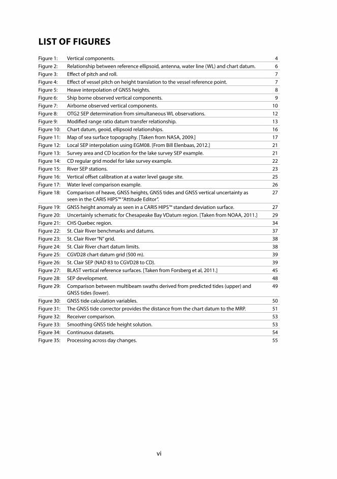
Figure 1: Vertical components. 4Figure 2: Relationship between reference ellipsoid, antenna, water line (WL) and chart datum. 6Figure 3: Effect of pitch and roll. 7Figure 4: Effect of vessel pitch on height translation to the vessel reference point. 7Figure 5: Heave interpolation of GNSS heights. 8Figure 6: Ship borne observed vertical components. 9Figure 7: Airborne observed vertical components. 10Figure 8: OTG2 SEP determination from simultaneous WL observations. 12Figure 9: Modified range ratio datum transfer relationship. 13Figure 10: Chart datum, geoid, ellipsoid relationships. 16Figure 11: Map of sea surface topography. [Taken from NASA, 2009.] 17Figure 12: Local SEP interpolation using EGM08. [From Bill Elenbaas, 2012.] 21Figure 13: Survey area and CD location for the lake survey SEP example. 21Figure 14: CD regular grid model for lake survey example. 22Figure 15: River SEP stations. 23Figure 16: Vertical offset calibration at a water level gauge site. 25Figure 17: Water level comparison example. 26Figure 18: Comparison of heave, GNSS heights, GNSS tides and GNSS vertical uncertainty as

seen in the CARIS HIPS™ “Attitude Editor”.27

Figure 19: GNSS height anomaly as seen in a CARIS HIPS™ standard deviation surface. 27Figure 20: Uncertainly schematic for Chesapeake Bay VDatum region. [Taken from NOAA, 2011.] 29Figure 21: CHS Quebec region. 34Figure 22: St. Clair River benchmarks and datums. 37Figure 23: St. Clair River “N” grid. 38Figure 24: St. Clair River chart datum limits. 38Figure 25: CGVD28 chart datum grid (500 m). 39Figure 26: St. Clair SEP (NAD 83 to CGVD28 to CD). 39Figure 27: BLAST vertical reference surfaces. [Taken from Forsberg et al, 2011.] 45Figure 28: SEP development. 48Figure 29: Comparison between multibeam swaths derived from predicted tides (upper) and

GNSS tides (lower).49

Figure 30: GNSS tide calculation variables. 50Figure 31: The GNSS tide corrector provides the distance from the chart datum to the MRP. 51Figure 32: Receiver comparison. 53Figure 33: Smoothing GNSS tide height solution. 53Figure 34: Continuous datasets. 54Figure 35: Processing across day changes. 55

vii

ACRONYMS

ADCIRC Advanced Circulation Model

ALB Airborne Lidar Bathymetry

ARP Antenna Reference Point

BAG Bathymetric Attributed Grid

BLAST Bringing Land and Sea Together, North Sea vertical datum project

CD Chart Datum

CGVD 28 Canadian Geodetic Vertical Datum 1928

CHS Canadian Hydrographic Service

CORS Continuously Operating Reference System (US NOAA)

CSRS Canadian Spatial Reference Stations

DD Dynamic Draft

EGG2008 European Gravimetric Geoid 2008

EGM Earth Gravity Model

ERS Ellipsoidally Referenced Surveying

FIG International Federation of Surveyors

Galileo European GNSS

GEOID US geoid/ellipsoid undulation models (…, 99, 03, 09, ..)

GLONASS Russian GNSS

GNSS Global Navigation Satellite System

GPS Global Positioning System (US GNSS)

GIPSY GNSS-Inferred Positioning System

GRS 80 Geodetic Reference System 1980

H Orthometric height

h Ellipsoid height

IGLD 85 International Great Lakes Datum 1985

IGS International GNSS System (effective 1/1/13). Note: IGS08=ITRF08

IMU Inertial Motion Unit

ITRF International Terrestrial Reference Frame

IGN International GNSS Service

LAT Lowest Astronomic Tide (International chart datum).

MDT or MDOT Mean Dynamic Ocean Topography

MLLW Mean Lower Low Water (US chart datum)

MLW Mean Low Water

MSL Mean Sea Level (average water level established from 19 years of observations)

MSS Mean Sea Surface

MTL Mean Tide Level

N Geoid/ellipsoid undulation

NAD 83 North American Datum 1983

NAVD 88 North American Vertical Datum 1988

NAVOCEANO Naval Oceanographic Office (US)

NGS National Geodetic Survey (US)

NOAA National Oceanic and Atmospheric Administration (US)

NSHC North Sea Hydrodynamic Committee

PPP Precise Point Positioning

PPK Post Processed Kinematic positioning

RP Reference Point

RTK Real-time Kinematic positioning

RTG Real-time GIPSY

SBET Smoothed Best Estimate Trajectory

SEP Separation model (vertical)

TCARI Tidal Constituent and Residual Interpolation

TIN Triangular Irregular Network (surface representation)

TPU Total Propagated Uncertainty

TSS Topography of the Sea Surface

UKHO United Kingdom Hydrographic Office

VDatum Vertical Datum Transformation (NOAA software tool)

VORF UKHO Vertical Offshore Reference Frame

EVREF2007 European Vertical Reference Frame 2007

WGS 84 World Geodetic System 1984

WL Water Level

viii

FOREWORD

The hydrographic surveying community is using high-accuracy Global Navigation Sat-ellite System (GNSS) positioning techniques for vertical positioning of survey platforms, the sea surface and the sea floor. This method of hydrographic surveying is known as Ellipsoidally Referenced Surveying (ERS). ERS provides a direct measurement of the sea floor to the ellipsoid, as established by GNSS observations, and a translation of the ref-erence from the ellipsoid to the geoid and/or a chart datum. In order to meet required vertical positioning standards, it is of paramount importance that the entire ERS pro-cess be thoroughly understood and that the appropriate procedures are in place dur-ing data acquisition, validation, cleaning and processing phases.

Many of the groups using ERS techniques have developed their internal Standard Op-erating Procedures (SOP) through in-house experience and trial-and-error testing. It is this wealth of group information that is being drawn upon to help develop a set of “best practices” for the hydrographic industry. The development of ERS best practices is being conducted by International Federation of Surveyors (FIG) working group 4.1 un-der Commission 4 and will be shared with the IHO for possible inclusion in International Hydrographic Organization (IHO) publication C13, Manual on Hydrography.

I would like to thank our working group chair, Mr. Jerry Mills, for leading this work and the working group technical lead, Dr. David Dodd, who was solely responsible for com-municating with the various contributing organizations, collating their comments and developing the majority of the manuscript. This is a significant contribution of these geomatics professionals to the wider objectives of the international hydrography com-munity, and as well to those of the FIG.

Dr. Michael Sutherland, Chair, FIG Commission 4

ix

PREFACE

This document has been developed from contributions from many hydrographic or-ganizations around the world and aims to provide a background that can be utilized by hydrographers to establish best practices for ERS. It looks at the relative importance of all of the vertical components associated with ERS, including; GNSS-based positioning of the antenna, translation of antenna position to the survey platform reference point per rigid body motion, and the application of heave and dynamic draft. Also discussed is the development of vertical-datum separation models used to translate the ERS in-formation to other datums, such as a geoid and a chart datum. Ten case studies are included to provide examples of how different groups are using ERS. The final chapter of the document provides a summary of the recommended best practices that the hy-drographic surveying community use for success in ERS work.

The Working Group is deeply indebted to the following organizations which assisted in compiling this document and their assistance is gratefully acknowledged:

– The Canadian Hydrographic Service (Service Hydrographic du Canada)

– The Swedish Maritime Administration

– The US National Oceanic and Atmospheric Administration (NOAA)

– The US Naval Oceanographic Office

– The Royal Australian Navy

– State Port Operators- Maritime Safety Queensland – Australia

– The United Kingdom Hydrographic Office

– The Netherlands Hydrographic Office

– Service Hydrographique et Oceanographique de la Marine (French Hydrograph-ic Office)

– Centro de Hidrografia da Marinha (Brazilian Navy)

– Instituto Hidrografico – Portugal

– Danish Maritime Safety Administration

– Finish Maritime Administration

– David Evans and Associates

– Fugro Geoservices

– Fugro-Pelagos.

Special thanks are given to CARIS, the University of New Brunswick (Ocean Mapping Group) and the University of Southern Mississippi (Hydrographic Science Research Center) in recognition of their financial support.

The following individuals are acknowledged for their responses to working group in-quiries and questionnaires which became the basis for the material in this document:

x

Stage 1 (Original contributors, 2009)

– Allen, C., G. Rice, and J. Mills. Personal Communication. US National Oceanic and At-mospheric Administration (NOAA)

– Arroyo-Suarez , E. Personal communication. US Naval Oceanographic Office

– Bartlett, J. Personal communication. Canadian Hydrographic Service (CHS) Central

– Battilana, D. Personal communication. Royal Australian Navy

– Church, I. Personal communication. The University of New Brunswick (UNB)

– Godin, A., D. Langelier, A. Biron, C. Comtois, F. Lavoie, and D. Lefaivre. Personal com-munication. Service Hydrographic du Canada, Quebec

– Gourley, M., A. Hoggarth and C. Collins. Personal Communications. CARIS

– Hare, R. Personal Communication. Canadian Hydrographic Service, Pacific

– Moyles, D. Personal communication. Fugro-Pelagos

– Olsson, U. Personal communication. Swedish Maritime Administration

– Parsons, S., G. Costello, C. O’Reilly and P. MacAulay. Personal communication. Cana-dian Hydrographic Service, Atlantic

Stage 2 (Questionnaire respondents, 2010)

– Bartlett, J. Canadian Hydrographic Service, Central

– Dorst, L. Netherlands Hydrographic Office

– Elenbaas, B. US Naval Oceanographic Office, Joint Airborne Lidar Bathymetry Techni-cal Center of Excellence

– Hocker, B. David Evans and Associates

– Jayaswal, Z. Australian Hydrographic Office, Royal Australian Navy

– Manteigas, L.P. Instituto Hidrografico – Portugal

– Moyles, D. Fugro-Pelagos

– Parker, D. United Kingdom Hydrographic Office

– Pastor, C. Fugro Geosservices

– Pineau-Guillou, L. Service Hydrographique et Oceanographique de la Marine (French Hydrographic Office)

– RAMOS, A.M. Geodesy Division, Centro de Hidrografia da Marinha, Brazilian Navy

– Riley, J. US National Oceanic and Atmospheric Administration

– Scarfe, B. University of Waikato, New Zealand

– Solvsten, M. Danish Maritime Safety Administration

– Varonen, J. Finnish Maritime Administration

Jerry Mills Dr. David Dodd Chair, FIG Working Group 4.1 Technical Lead, FIG Working Group 4.1

1

1 INTRODUCTION

One of the most significant issues in hydrography today is using the ellipsoid as the vertical reference for surveying measurements. High-accuracy GNSS is used to position (vertically) hydrographic data acquisition platforms, relating bathymetric observations and elevations of conspicuous land features directly to the ellipsoid. Models are then used to translate those observations to another datum. The use of high-accuracy verti-cal GNSS and transformation models to replace (in effect) traditional tidal correctors is relatively new to the hydrographic community and, as such, requires some discus-sion. Even though individual components of the process are well understood in their particular field, it is their amalgamation and application to hydrography that requires explanation, clarification and evaluation.

Hydrographic surveying has traditionally been conducted solely for the purpose of creating nautical charts for safety of navigation. It now encompasses a multitude of methods and applications in the marine environment, and has a vital role in coastal zone management. The coastal zone encompasses a wide swath along the shoreline that includes both the land and sea, and properly merging information from the two is essential for the analysis of coastal processes and sound management decisions. Verti-cal land (topography) and ocean (bathymetry) data are often collected for different purposes, using different methods and related to different vertical reference surfaces. The need to merge the two data types drives the need to resolve these differences.

One surface that is used in modern data acquisition on both land and sea is a geometric reference ellipsoid. Traditionally, reference ellipsoids were used to define horizontal da-tums. With the emergence of high-accuracy GNSS, reference ellipsoids are being used as a vertical reference surface to which ellipsoid heights both on land and at sea can be related making the merging of the two types of data a trivial process (ref: FIG Publica-tion No. 37). Although these reference ellipsoids are convenient, they are not physical surfaces, such as those defined by gravity (geodetic datum) or a water level surface (tidal datum). Therefore, for analysis and map/chart production, GNSS-derived vertical infor-mation must be translated, using some combination of gridded data and modeling.

The FIG, under Commission 4, established working group 4.1 to develop “best practices” for Ellipsoidally Referenced Surveying (ERS). In a series of papers (Dodd et. al., 2010, Dodd and Mills, 2011 and Dodd and Mills 2012) working group members have outlined the is-sues associated with ERS and discussed the technical survey aspects of data acquisition and processing as well as the application of separation models as the final step in the pro-cess. As hydrographic organizations move forward with the use of ERS, the development and validation of separation models is, by far, providing the greatest challenge.

Some of the issues involved in Ellipsoidally Referenced Surveying include:

1. Data acquisition, in particular high accuracy (HA) GNSS

2. HA GNSS Data processing

3. Vertical separation model (SEP) development and application

4. QA/QC of vertical offsets, HA GNSS, motion and SEP

5. Uncertainty associated with vertical offsets, GNSS, motion and SEP

6. Data archive reference.

2

This publication expands and updates the discussion presented in FIG Publication 37 (FIG, 2006). Where FIG Publication 37 presents all of the aspects of ellipsoidally refer-enced surveying in general terms, this document explores these aspects in greater de-tail and offers recommendations for “best practices”. It also presents several case stud-ies as examples. The information presented here has been gathered from a wide variety of ERS practitioners and experts from around the world, with the intention of providing those just breaking into the field with a solid foundation for the development of their own procedures.

Notes: Throughout this discussion the separation model refers to a low water chart da-tum. However, any separation model system should include high water vertical refer-ence surfaces as well.

The term “water level gauge” will be used instead of the more commonly used term “tide gauge” to more accurately describe what is being measured.

This document is divided into 7 chapters. Following the introduction is a chapter on vertical positioning that reviews all of the components that go into deriving a final charted depth when using ERS techniques. Chapter 3 looks at the issues involved in developing a separation model and Chapters 4 and 5 look at quality control and uncer-tainty. Chapter 6 contains a series of case studies that provide real world examples. The final chapter outlines recommendations and a list of “best practices”.

3

2 VERTICAL POSITIONING

In order to conduct ERS in the marine environment, several issues must be addressed. The first is the GNSS position of the antenna, which must be determined using high-ac-curacy techniques. That position must then be translated to the vessel reference point (RP). This vessel RP height is then used to reference the seabed directly to the ellipsoid. In order to give the seabed value real physical meaning, the depth must be translated to a physical datum (geoid, mean sea level, chart datum…). The seabed depths must be referenced to a known and repeatable common datum to facilitate merging with other data (land or sea). A complete evaluation and recording of the propagation of uncertainties through the entire process is essential for a meaningful data analysis and the creation of products both now and in the future.

In order to understand the issues surrounding surveying to the ellipsoid it is necessary to understand the various contributors to the process. The following sections briefly describe:

1. Vertical components

2. High-accuracy GNSS

3. Effect of pitch, roll and heading

4. Heave

5. Shipborne derived depths

6. Airborne derived depths

7. Water levels

8. Vertical datums

9. Ellipsoid to chart datum

10. Translation to chart datum.

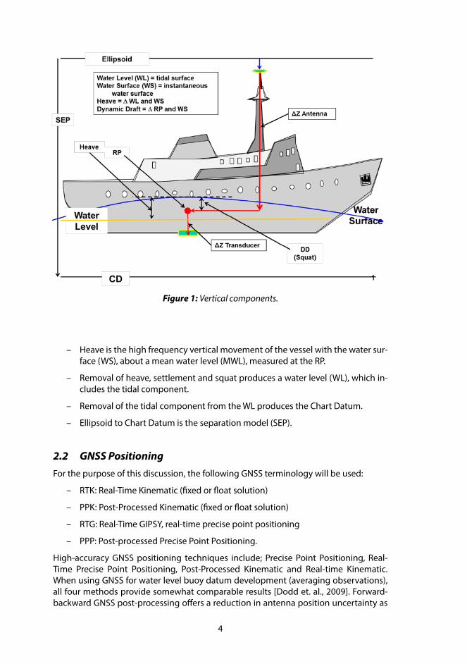
2.1 Vertical ComponentsThe following list describes the terminology associated with the vertical components of hydrographic surveying with respect to the ellipsoid (see Figure 1).

– Observed GNSS height is the distance from the ellipsoid to the receiving an-tenna phase center.

– ∆Z Antenna is the vertical offset between the antenna phase center and the ves-sel reference point (RP).

– ∆Z Transducer is the vertical offset between the RP and transducer.

– Observed depth is from transducer to bottom.

– Dynamic draft (DD), or settlement and squat, is the change in the survey plat-form vertical position in the water (water surface to RP) due to relative speed through the water.

4

– Heave is the high frequency vertical movement of the vessel with the water sur-face (WS), about a mean water level (MWL), measured at the RP.

– Removal of heave, settlement and squat produces a water level (WL), which in-cludes the tidal component.

– Removal of the tidal component from the WL produces the Chart Datum.

– Ellipsoid to Chart Datum is the separation model (SEP).

2.2 GNSS PositioningFor the purpose of this discussion, the following GNSS terminology will be used:

– RTK: Real-Time Kinematic (fixed or float solution)

– PPK: Post-Processed Kinematic (fixed or float solution)

– RTG: Real-Time GIPSY, real-time precise point positioning

– PPP: Post-processed Precise Point Positioning.

High-accuracy GNSS positioning techniques include; Precise Point Positioning, Real-Time Precise Point Positioning, Post-Processed Kinematic and Real-time Kinematic. When using GNSS for water level buoy datum development (averaging observations), all four methods provide somewhat comparable results [Dodd et. al., 2009]. Forward-backward GNSS post-processing offers a reduction in antenna position uncertainty as

Figure 1: Vertical components.

5

compared with the comparable technique’s real-time solution (RTK->PPK, RTG->PPP). Inaccuracies present in the backward solution are in general comparable to those in the forward solution (= real-time solution). The two temporal solutions amount to a repeated (independent) measurement wherein the uncertainty in the mean is lower in accordance with basic statistics (variance is halved; standard deviation is less by a fac-tor of 1/sqrt(2)). Additional positioning accuracy and robustness is achieved through inertial-aided GNSS technology, which may be leveraged in both real-time and post-processing scenarios. For bathymetry, where epoch-to-epoch solutions are necessary, the type of positioning should be identified to allow for the assignment of uncertainty. The vertical uncertainty associated with the GNSS heights will propagate directly into the uncertainty in the depth estimates. Regardless of the processing technique, it is suggested that raw GNSS observations be recorded at all times. If using real-time meth-ods, post-processing of all or a portion of the data can be used for quality control. Post-processing can also be used in the event of an interruption in real-time computations.

When using GNSS for water level buoy datum development (averaging observations), all four methods provide comparable results [Dodd et. al., 2009]. For bathymetry, where epoch-to-epoch solutions are necessary, the type of positioning should be identified to allow for the assignment of uncertainty. The vertical uncertainty associated with the GNSS heights will propagate directly into the uncertainty in the depth estimates. Re-gardless of the processing technique, it is suggested that raw GNSS observations be recorded at all times. If using real-time methods, post-processing of all or a portion of the data can be used for quality control. Post-processing can also be used in the event of an interruption in real-time computations.

High-accuracy GNSS for dynamic positioning in the vertical is relatively new to the hydrographic community. In the past, the vertical relationship between the GNSS an-tenna and the transducer was important, but not vital. Now, with the determination of bathymetry through GNSS vertical positioning, it is essential that all aspects related to the measurement of that position be understood and dealt with appropriately. All measurement uncertainty will propagate directly into the final depth. Total uncertainty resulting from the use of GNSS heights includes:

– The uncertainty in the GNSS vertical position of the antenna phase center.

– The measurement of the three dimensional offsets between the phase center and transducer.

– The translation of the vertical position to the transducer (or reference point), taking into account accuracy of the motion sensor(s).

High-accuracy GNSS in hydrographic surveying has two basic applications; bathym-etric data acquisition and chart datum development. For bathymetric data acquisi-tion, GNSS observations at the antenna are related directly to the depth observations through vessel offset measurements, thus providing a direct measurement from the ellipsoid to the sea floor. All vertical movement of the vessel, including water levels, heave, static and dynamic draft are included in the GNSS height observation. Chart datums can be established from GNSS water level buoys to estimate the mean water surface at a point relative to the ellipsoid. This separation can be used to translate the ellipsoid related bathymetric data to chart datum with varying degrees of accuracy.

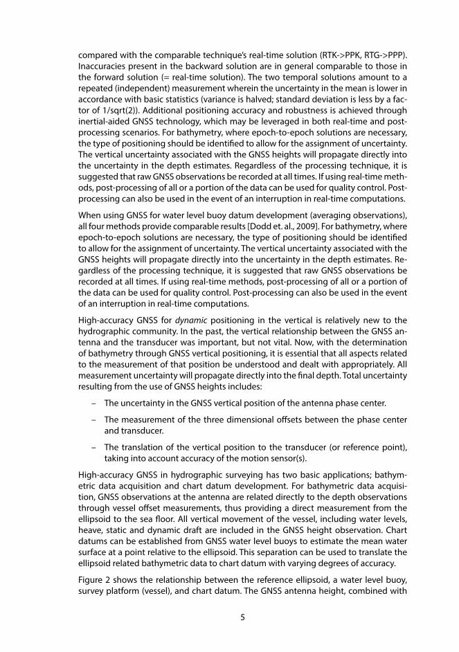
Figure 2 shows the relationship between the reference ellipsoid, a water level buoy, survey platform (vessel), and chart datum. The GNSS antenna height, combined with

6

its antenna to waterline distance (or “air draft”), provides the water surface measure-ments for datum determination in relation to a shore-based water level gauge. The datum-to-ellipsoid relationship is represented by a separation (SEP) model. The vessel GNSS height is connected to the depth observation through the “Z” offset. Although this offset is shown here as a single value, it actually varies with the pitch and roll of the vessel. The vessel air draft (antenna to waterline), taking into account all vessel motion, including heave, pitch, roll, long term static draft and dynamic draft, can be used to validate water level observations and datum determinations.

Water level buoys can be used to establish a chart datum in the area of a small survey or otherwise provide a check of a more expansive SEP model at a given point. Ideally, a water level transfer from a water level gauge in the area, with an established datum, is used to determine the datum at the buoy. Only long period buoy movement caused by the tides is required; therefore, the short term movement, such as heave, can be filtered out through averaging. A critical component for the establishment of a datum using a GNSS water level buoy is the waterline determination (distance from antenna to water line). Any error in the measurement of this offset will translate directly into the datum.

Water level buoys can also be used to validate and strengthen hydrodynamic models by providing water level observations away from the shore. Carefully calibrated and positioned (with respect to the ellipsoid) bottom mounted gauges can be used in lieu of the GPS buoy.

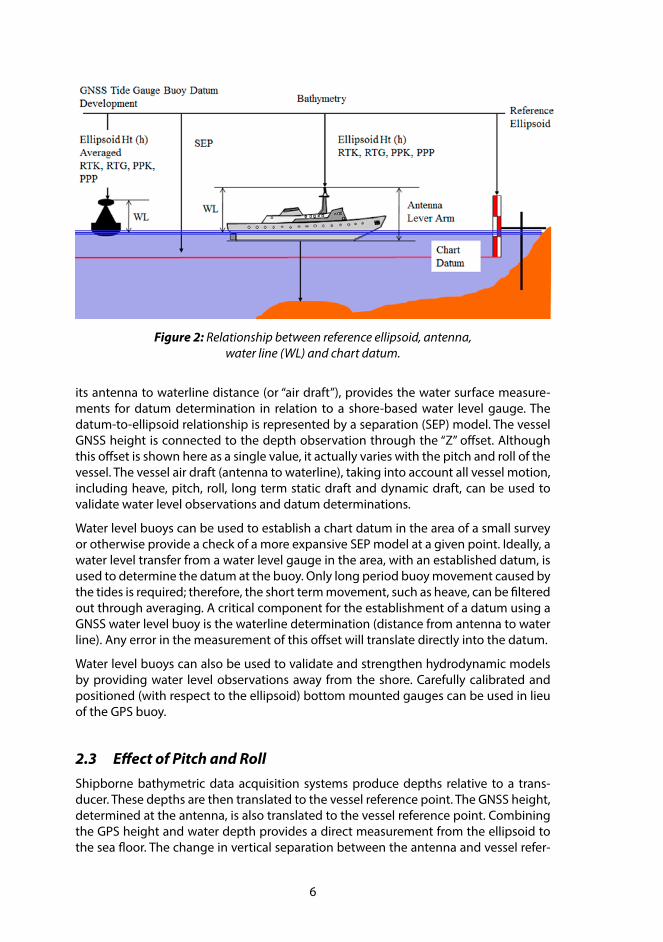
2.3 Effect of Pitch and RollShipborne bathymetric data acquisition systems produce depths relative to a trans-ducer. These depths are then translated to the vessel reference point. The GNSS height, determined at the antenna, is also translated to the vessel reference point. Combining the GPS height and water depth provides a direct measurement from the ellipsoid to the sea floor. The change in vertical separation between the antenna and vessel refer-

Figure 2: Relationship between reference ellipsoid, antenna, water line (WL) and chart datum.

7

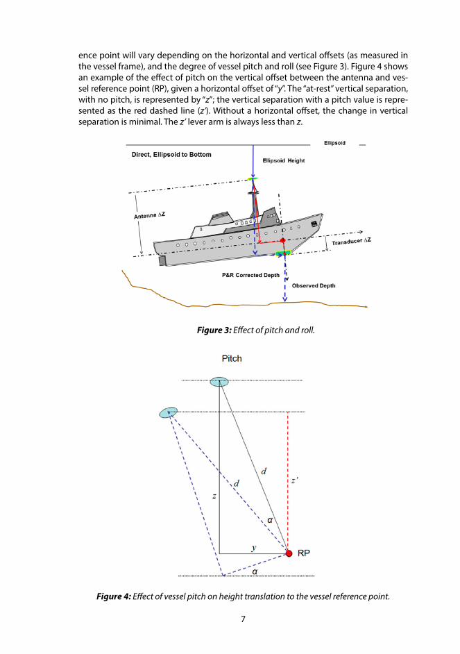
ence point will vary depending on the horizontal and vertical offsets (as measured in the vessel frame), and the degree of vessel pitch and roll (see Figure 3). Figure 4 shows an example of the effect of pitch on the vertical offset between the antenna and ves-sel reference point (RP), given a horizontal offset of “y”. The “at-rest” vertical separation, with no pitch, is represented by “z”; the vertical separation with a pitch value is repre-sented as the red dashed line (z’). Without a horizontal offset, the change in vertical separation is minimal. The z’ lever arm is always less than z.

Figure 3: Effect of pitch and roll.

Figure 4: Effect of vessel pitch on height translation to the vessel reference point.

8

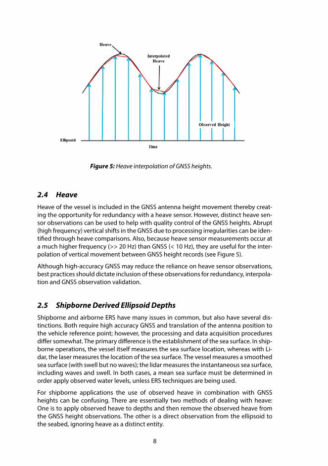
2.4 HeaveHeave of the vessel is included in the GNSS antenna height movement thereby creat-ing the opportunity for redundancy with a heave sensor. However, distinct heave sen-sor observations can be used to help with quality control of the GNSS heights. Abrupt (high frequency) vertical shifts in the GNSS due to processing irregularities can be iden-tified through heave comparisons. Also, because heave sensor measurements occur at a much higher frequency (>> 20 Hz) than GNSS (< 10 Hz), they are useful for the inter-polation of vertical movement between GNSS height records (see Figure 5).

Although high-accuracy GNSS may reduce the reliance on heave sensor observations, best practices should dictate inclusion of these observations for redundancy, interpola-tion and GNSS observation validation.

2.5 Shipborne Derived Ellipsoid DepthsShipborne and airborne ERS have many issues in common, but also have several dis-tinctions. Both require high accuracy GNSS and translation of the antenna position to the vehicle reference point; however, the processing and data acquisition procedures differ somewhat. The primary difference is the establishment of the sea surface. In ship-borne operations, the vessel itself measures the sea surface location, whereas with Li-dar, the laser measures the location of the sea surface. The vessel measures a smoothed sea surface (with swell but no waves); the lidar measures the instantaneous sea surface, including waves and swell. In both cases, a mean sea surface must be determined in order apply observed water levels, unless ERS techniques are being used.

For shipborne applications the use of observed heave in combination with GNSS heights can be confusing. There are essentially two methods of dealing with heave: One is to apply observed heave to depths and then remove the observed heave from the GNSS height observations. The other is a direct observation from the ellipsoid to the seabed, ignoring heave as a distinct entity.

Figure 5: Heave interpolation of GNSS heights.

9

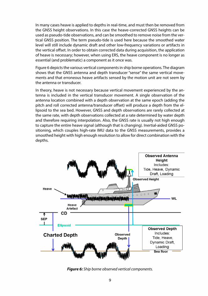
In many cases heave is applied to depths in real-time, and must then be removed from the GNSS height observations. In this case the heave-corrected GNSS heights can be used as pseudo-tide observations, and can be smoothed to remove noise from the ver-tical GNSS position. The term pseudo-tide is used here because the smoothed water level will still include dynamic draft and other low-frequency variations or artifacts in the vertical offset. In order to obtain corrected data during acquisition, the application of heave is necessary; however, when using ERS, the heave component is no longer as essential (and problematic) a component as it once was.

Figure 6 depicts the various vertical components in ship borne operations. The diagram shows that the GNSS antenna and depth transducer “sense” the same vertical move-ments and that erroneous heave artifacts sensed by the motion unit are not seem by the antenna or transducer.

In theory, heave is not necessary because vertical movement experienced by the an-tenna is included in the vertical transducer movement. A single observation of the antenna location combined with a depth observation at the same epoch (adding the pitch and roll corrected antenna/transducer offset) will produce a depth from the el-lipsoid to the sea bed. However, GNSS and depth observations are rarely collected at the same rate, with depth observations collected at a rate determined by water depth and therefore requiring interpolation. Also, the GNSS rate is usually not high enough to capture the entire heave signal (although that is changing). Inertial-aided GNSS po-sitioning, which couples high-rate IMU data to the GNSS measurements, provides a smoothed height with high enough resolution to allow for direct combination with the depths.

Figure 6: Ship borne observed vertical components.

10

ERS allows for the reduced sounding solution to be produced without direct impact from draft, loading draft, and dynamic draft (settlement and squat), and potentially without direct impact from heave. Although in general, draft, loading draft, dynamic draft and distinct heave observations remain necessary to determine the location of the transducer within the water column for precise ray tracing calculations and to re-trieve the actual water surface. One significant advantage of retrieving the water sur-face is that it allows for a comparison with traditional tidal techniques. The ellipsoid-to-water surface observations also provide validation for hydrodynamic models.

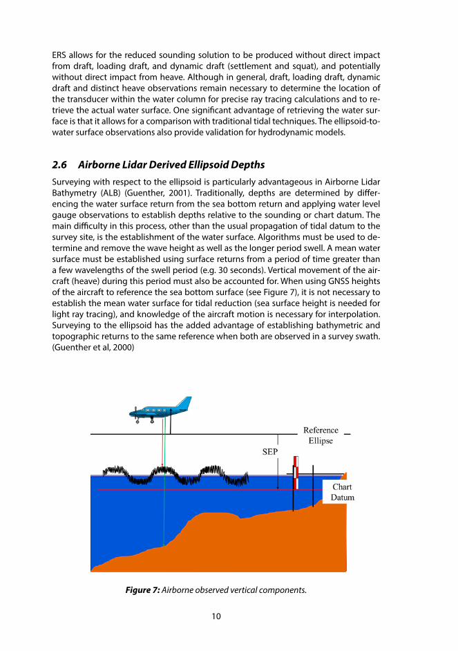
2.6 Airborne Lidar Derived Ellipsoid DepthsSurveying with respect to the ellipsoid is particularly advantageous in Airborne Lidar Bathymetry (ALB) (Guenther, 2001). Traditionally, depths are determined by differ-encing the water surface return from the sea bottom return and applying water level gauge observations to establish depths relative to the sounding or chart datum. The main difficulty in this process, other than the usual propagation of tidal datum to the survey site, is the establishment of the water surface. Algorithms must be used to de-termine and remove the wave height as well as the longer period swell. A mean water surface must be established using surface returns from a period of time greater than a few wavelengths of the swell period (e.g. 30 seconds). Vertical movement of the air-craft (heave) during this period must also be accounted for. When using GNSS heights of the aircraft to reference the sea bottom surface (see Figure 7), it is not necessary to establish the mean water surface for tidal reduction (sea surface height is needed for light ray tracing), and knowledge of the aircraft motion is necessary for interpolation. Surveying to the ellipsoid has the added advantage of establishing bathymetric and topographic returns to the same reference when both are observed in a survey swath. (Guenther et al, 2000)

Figure 7: Airborne observed vertical components.

11

2.7 Water LevelsWhen using GNSS heights to remove the vertical vessel movement, traditional water level gauges are no longer necessary for the reduction of observed depths. Instead, separation models are used to transform the depths from the ellipsoid to chart datum. However, water level gauge observations during surveys are still necessary in order to validate the models, for quality control of the GNSS heights and to provide redundancy in the event of high-accuracy GNSS dropouts. Shore based water level gauges are also used to establish chart datum at GNSS water level buoy or bottom mounted gauge lo-cated at the survey site. Establishing chart datum at offshore locations helps to anchor separation models.

2.7.1 Traditional Tidal Datums and Tidal ZoningChart datums are used as the vertical reference for water depths on nautical charts and are chosen such that the water surface will not usually fall below it. The international standard for chart datums is Lowest Astronomic Tide (LAT) but different chart datums continue to be used by various nations. Most of these tidal datums are computed over specific 19 year periods called tidal datum epochs.

In the coastal waters of the United States, Mean Lower Low Water (MLLW) is used as the chart datum. It is computed by averaging the observed height of the lower low water for each tidal day over a 19 year period. The Chart Datum for Canadian charts is Lower Low Water Large Tide which is the average of the observed lowest low waters, one from each of 19 years of observations. LAT, on the other hand, is based on the “predicted” lowest tide expected to occur in a 19 year period. This prediction is made by perform-ing a harmonic analysis of the water level observations at a particular location, then using the resulting harmonic constituents to predict the elevation of the lowest tide that will occur over a 19 year period.

It is clear that installing and maintaining tide/water level gauges continuously for 19 years is difficult and expensive so the number of such primary gauges is limited in num-ber. However, supplemental shorter term gauges can be installed to geographically densify the points of water level data acquisition. In most cases, not enough water level stations can be installed in a practical sense to provide direct control to all areas of a hydrographic survey. Hence, tide and water level zoning must be used to extrapolate or interpolate the tide and water level variations from those water level stations closest to the survey area. Zoning uncertainty can be reduced by increasing the number of sta-tions in the survey area. However, the desire for more stations must be balanced with higher cost and increased logistical complexity.

Any zoning scheme requires an oceanographic study of the water level variations in the survey area. For tidal areas, co-tidal maps of the time and range of tide are constructed based on historical data, hydrodynamic models and other information sources. Based on how fast the time and range of tide progress through a given survey area, the co-tidal lines are used to delineate discrete geospatial zones of equal time and range of tide. Once this is constructed, time and range correctors to appropriate operational stations or tide prediction stations can be calculated.

12

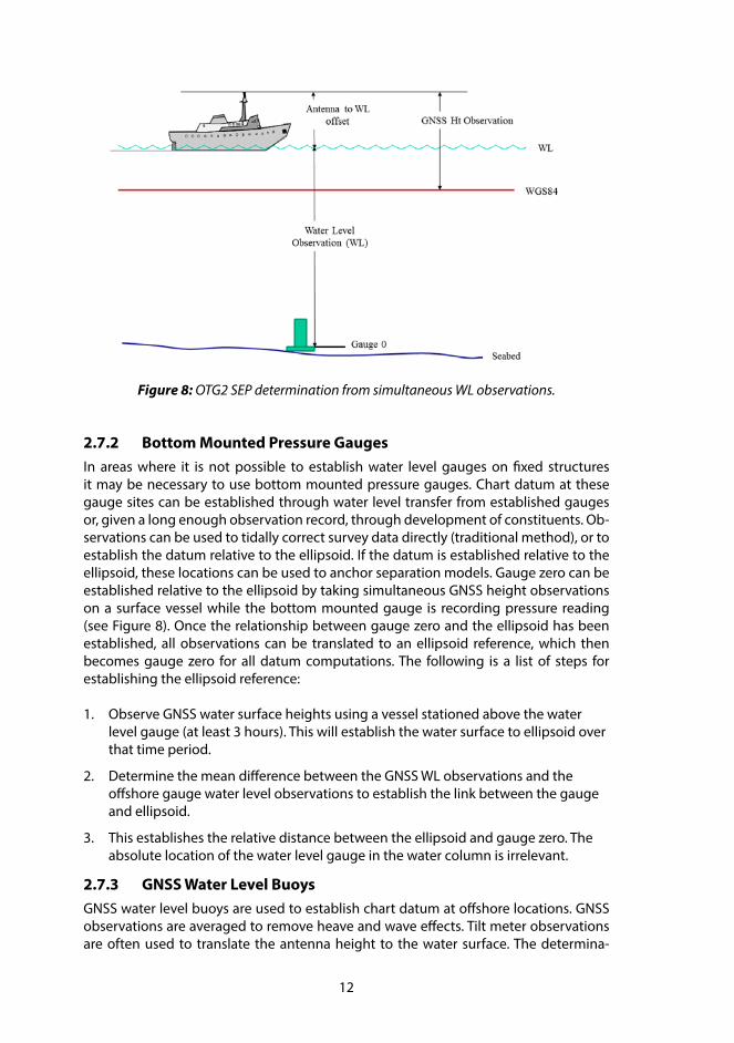
2.7.2 Bottom Mounted Pressure GaugesIn areas where it is not possible to establish water level gauges on fixed structures it may be necessary to use bottom mounted pressure gauges. Chart datum at these gauge sites can be established through water level transfer from established gauges or, given a long enough observation record, through development of constituents. Ob-servations can be used to tidally correct survey data directly (traditional method), or to establish the datum relative to the ellipsoid. If the datum is established relative to the ellipsoid, these locations can be used to anchor separation models. Gauge zero can be established relative to the ellipsoid by taking simultaneous GNSS height observations on a surface vessel while the bottom mounted gauge is recording pressure reading (see Figure 8). Once the relationship between gauge zero and the ellipsoid has been established, all observations can be translated to an ellipsoid reference, which then becomes gauge zero for all datum computations. The following is a list of steps for establishing the ellipsoid reference:

1. Observe GNSS water surface heights using a vessel stationed above the water level gauge (at least 3 hours). This will establish the water surface to ellipsoid over that time period.

2. Determine the mean difference between the GNSS WL observations and the offshore gauge water level observations to establish the link between the gauge and ellipsoid.

3. This establishes the relative distance between the ellipsoid and gauge zero. The absolute location of the water level gauge in the water column is irrelevant.

2.7.3 GNSS Water Level BuoysGNSS water level buoys are used to establish chart datum at offshore locations. GNSS observations are averaged to remove heave and wave effects. Tilt meter observations are often used to translate the antenna height to the water surface. The determina-

Figure 8: OTG2 SEP determination from simultaneous WL observations.

13

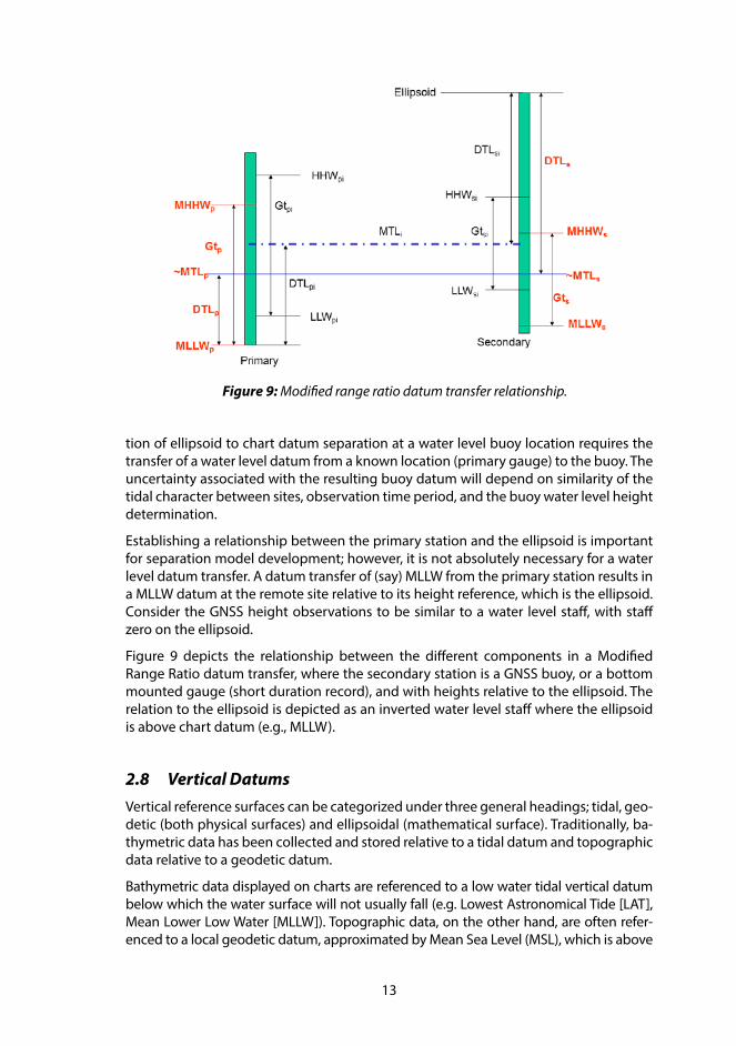
tion of ellipsoid to chart datum separation at a water level buoy location requires the transfer of a water level datum from a known location (primary gauge) to the buoy. The uncertainty associated with the resulting buoy datum will depend on similarity of the tidal character between sites, observation time period, and the buoy water level height determination.

Establishing a relationship between the primary station and the ellipsoid is important for separation model development; however, it is not absolutely necessary for a water level datum transfer. A datum transfer of (say) MLLW from the primary station results in a MLLW datum at the remote site relative to its height reference, which is the ellipsoid. Consider the GNSS height observations to be similar to a water level staff, with staff zero on the ellipsoid.

Figure 9 depicts the relationship between the different components in a Modified Range Ratio datum transfer, where the secondary station is a GNSS buoy, or a bottom mounted gauge (short duration record), and with heights relative to the ellipsoid. The relation to the ellipsoid is depicted as an inverted water level staff where the ellipsoid is above chart datum (e.g., MLLW).

2.8 Vertical DatumsVertical reference surfaces can be categorized under three general headings; tidal, geo-detic (both physical surfaces) and ellipsoidal (mathematical surface). Traditionally, ba-thymetric data has been collected and stored relative to a tidal datum and topographic data relative to a geodetic datum.

Bathymetric data displayed on charts are referenced to a low water tidal vertical datum below which the water surface will not usually fall (e.g. Lowest Astronomical Tide [LAT], Mean Lower Low Water [MLLW]). Topographic data, on the other hand, are often refer-enced to a local geodetic datum, approximated by Mean Sea Level (MSL), which is above

Figure 9: Modified range ratio datum transfer relationship.

14

LAT and MLLW. A geodetic datum is a surface that varies with gravity (geoid). MSL is a surface that varies from the geoid due to sea surface topography (see section 2.9.1). The chart datum surface varies from MSL due to the effects of tides and ocean dynamics.

GPS derived heights must be transformed from the reference ellipsoid to the geoid or chart datum. In some cases, data sets can be adjusted by simply applying a constant offset. In other cases it is necessary to apply more complex algorithms taking into ac-count sea surface topography and hydrodynamic ocean models.

2.8.1 Geodetic Vertical DatumWhen the height of an object is expressed it must be related to something. The height of a ceiling is relative to the floor. The height of a building is relative to the ground out-side. The elevation of a mountain is relative to Mean Sea Level (MSL). The expression MSL, when applied to elevation, usually refers to the height above the local geodetic datum. The Canadian Geodetic Vertical Datum (CGVD28) and the USA North American Vertical Datum (NAVD88) are referenced to MSL at Rimouski, Quebec. These systems are realized through the physical monuments in the ground, and they move with the continental plates. The elevations of all reference marks (bench marks) within the two systems are related to MSL at Rimouski through precise leveling and gravity observa-tions. These geodetic vertical reference datums do not coincide with observed MSL at any other location due to local atmospheric and oceanographic effects.

Natural Resources Canada (NRCan) recently released the Canadian Geodetic Vertical Da-tum of 2013 (CGVD2013), which is the new standard to reference heights in Canada. This new height reference system is replacing the Canadian Geodetic Vertical Datum of 1928 (CGVD28). CGVD2013 is defined by the equipotential surface (Wo = 62,636,856.0 m2 s-2). This new vertical datum is realized by the geoid model CGG2013, which provides the sep-aration between the GRS80 ellipsoid and the above described surface in NAD83(CSRS) reference frame, making it compatible with GNSS. CGVD2013 heights obtained from GNSS and geoid model CGG2013 prevail over the published elevations, making the geoid model the primary realization of the vertical datum rather than the physical benchmarks.

The geoid is a surface of equal gravity potential and is used to approximate the shape of the earth. The geoid coincides approximately with MSL and is represented by a geodet-ic vertical reference datum, as discussed above. If there were no long term atmospheric or oceanographic effects (e.g. prevailing winds and currents), then MSL determined over a long period (~19 years) would coincide with geoid. In reality, determination of MSL at a location will vary from the geoid by up to ±1 metre. This variation is known as sea surface (or ocean) topography.

2.8.2 Chart Datum (CD)Chart datums (CD) are used on nautical charts to reference water depths. Traditionally, bathymetric data has been collected relative to a survey (or sounding) datum, then translated to chart datum for storage and chart production. As a result, most legacy bathymetric depth data are relative to some local chart datum.

The following is a listing of some chart datum definitions:

MLW Mean Low Water

MLLWLT Mean Lower Low Water Large Tide

15

MLLW Mean Lower Low Water

LNT Lowest Normal Tide

LLWLT Lower Low Water Large Tide

LAT Lowest Astronomic Tide (atmospheric and oceanographic effects mini-mized)

Chart datums are only fully valid at the location where the tides are observed. Even if MSL is the same at two locations (relative to the geoid), the low water chart datum will likely be different. One of the most significant challenges in traditional hydrog-raphy is establishing the relationship between the instantaneous water surface and chart datum away from water level gauge locations. Tidal correctors are measured at water level gauge locations and then translated to the survey site through co-tidal charts or tide zoning. Uncertainty in the relationship between the instantaneous wa-ter surface and CD at the survey site is a significant component of the overall depth uncertainty.

2.8.3 Reference EllipsoidThe shape of the geoid can be approximated by a three-dimensional ellipse (ellipsoid). Because the earth is symmetric about the poles, the ellipsoid can be defined with a bi-axial ellipse, with the semi-minor axis aligned with the earth’s axis of rotation and the semi-major axis aligned with the equatorial plane. This mathematical representation of the earth allows for relatively simple geographic (latitude, longitude and height) posi-tion computations. The vertical relationship between the ellipsoid, geoid and terrain is:

h = H + N

Where:

h = ellipsoid height

H = orthometric height

N = geoid height, also known as the geoid/ellipsoid undulation

The reference ellipsoid does not define a datum, it simply defines the parameters of the ellipse. A combination of the ellipsoid and its location with respect to the earth, defines a datum.

GNSS heights are determined relative to the mathematically defined ellipsoid. These heights must be translated to the geoid, through a geoid height model, in order to give them a physical relationship to the earth. Geoid models are determined through satellite observations as well as GNSS and gravity observations. These geoid/ellipsoid separation models can be established using land based techniques including GNSS ob-servations, leveling and gravity observations. They can also be established using space based techniques with specifically designed and tasked gravimetric satellites. Some existing models are GEOID96, 99, 03, 08, 12a and EGM96 and 08. It should be noted that the GEOID series of models define the separation between NAD83 and NAVD88, the realizations of which are sometimes referred to as a hybrid geoid (in contrast to the purely gravimetric geoid).

As more information is being collected through GNSS observations the ellipsoid is be-coming more popular as the reference surface for all information. This mathematical

16

surface will, over time, change the least of the three vertical datum types. Translation between the geoid and chart datums is accomplished through surface models. As the relationships between the different surfaces changes or becomes better established, the models can be updated without affecting the base data.

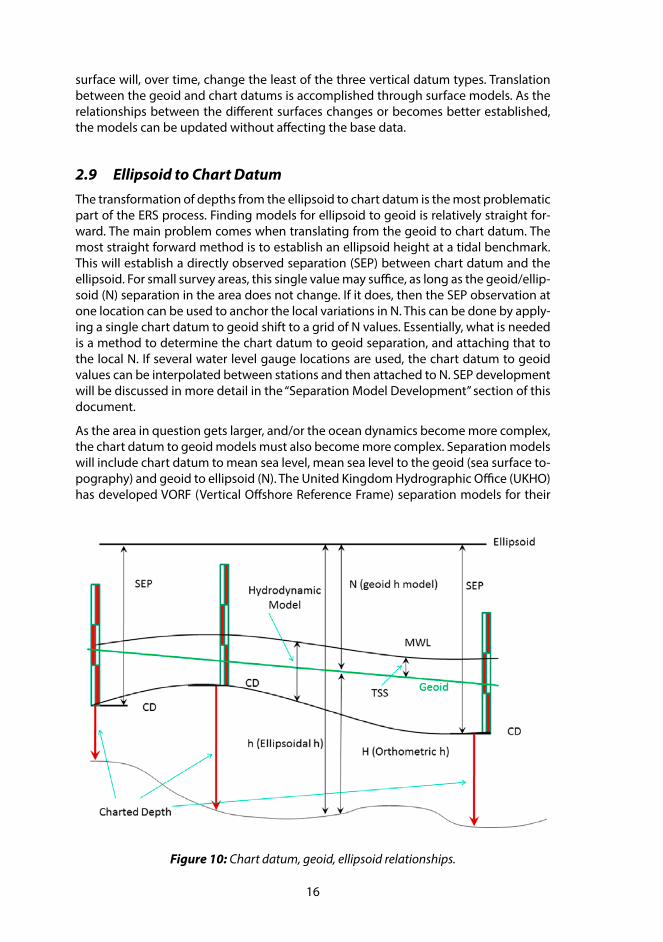
2.9 Ellipsoid to Chart DatumThe transformation of depths from the ellipsoid to chart datum is the most problematic part of the ERS process. Finding models for ellipsoid to geoid is relatively straight for-ward. The main problem comes when translating from the geoid to chart datum. The most straight forward method is to establish an ellipsoid height at a tidal benchmark. This will establish a directly observed separation (SEP) between chart datum and the ellipsoid. For small survey areas, this single value may suffice, as long as the geoid/ellip-soid (N) separation in the area does not change. If it does, then the SEP observation at one location can be used to anchor the local variations in N. This can be done by apply-ing a single chart datum to geoid shift to a grid of N values. Essentially, what is needed is a method to determine the chart datum to geoid separation, and attaching that to the local N. If several water level gauge locations are used, the chart datum to geoid values can be interpolated between stations and then attached to N. SEP development will be discussed in more detail in the “Separation Model Development” section of this document.

As the area in question gets larger, and/or the ocean dynamics become more complex, the chart datum to geoid models must also become more complex. Separation models will include chart datum to mean sea level, mean sea level to the geoid (sea surface to-pography) and geoid to ellipsoid (N). The United Kingdom Hydrographic Office (UKHO) has developed VORF (Vertical Offshore Reference Frame) separation models for their

Figure 10: Chart datum, geoid, ellipsoid relationships.

17

coastal waters (see Adams, 2006). The National Oceanic and Atmospheric Administra-tion (NOAA) had developed VDatum for much of the USA coastal waters (see Gesch and Wilson, 2001). VDatum and VORF will be discussed in more detail in the “Case Studies” section of this document.

Of particular importance to the hydrographic community is total propagated uncer-tainty (TPU). TPU models have been developed for all aspect of the ERS process except for the SEP translation process. A discussion of TPU and VDatum can be found at the NOAA website: http://vdatum.noaa.gov/docs/est_uncertainties.html

Figure 10 depicts the relationship between chart datum (CD), the geoid and the el-lipsoid. The ellipsoid is depicted as the primary reference (horizontal line) and all other surfaces are shown with respect to it. “SEP” refers to the CD to ellipsoid separation at water level gauge locations, which are depicted as water level staffs in the figure. The geoid is shown as a straight sloping line; again, with respect to the ellipsoid. MSL and MLW are shown as undulating lines with similar but different trends. This is meant to indicate that they are closely related, but their separation will differ from place to place. This difference is represented by the hydrodynamic model. The separation between the geoid and MSL is shown as topography of the sea surface (TSS).

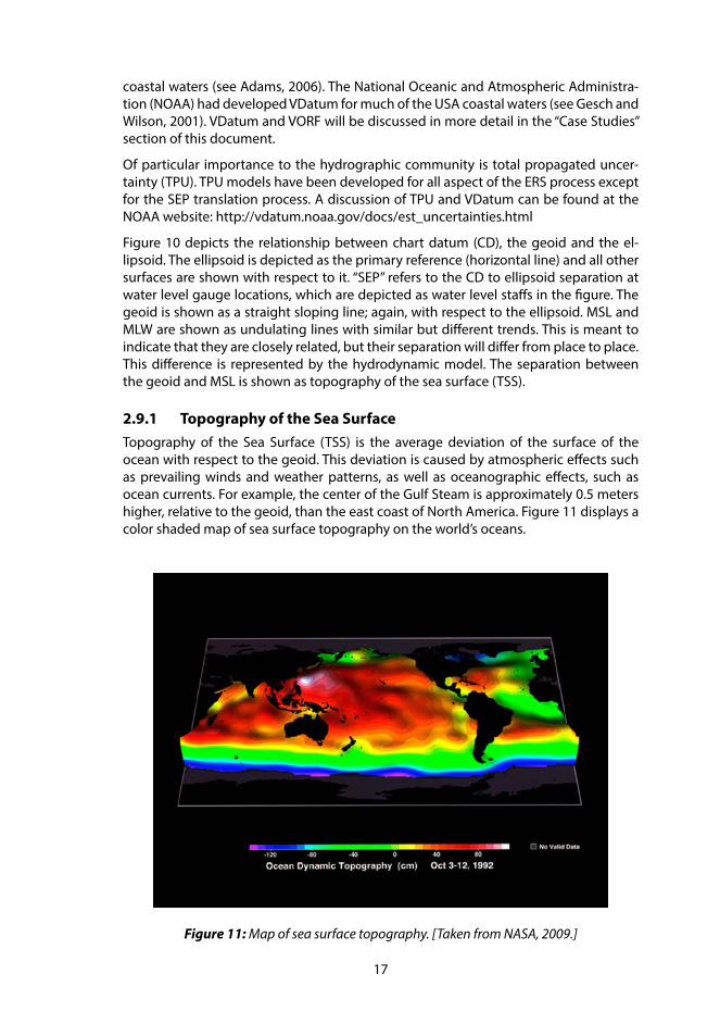
2.9.1 Topography of the Sea SurfaceTopography of the Sea Surface (TSS) is the average deviation of the surface of the ocean with respect to the geoid. This deviation is caused by atmospheric effects such as prevailing winds and weather patterns, as well as oceanographic effects, such as ocean currents. For example, the center of the Gulf Steam is approximately 0.5 meters higher, relative to the geoid, than the east coast of North America. Figure 11 displays a color shaded map of sea surface topography on the world’s oceans.

Figure 11: Map of sea surface topography. [Taken from NASA, 2009.]

18

TSS can be determined at water level gauges where MSL has been observed and the geodetic datum tied in through leveling. Alternatively, the geoid can be established relative to the reference ellipsoid through the geoid model, which requires establish-ment of the ellipsoid height at the water level gauge through GNSS observations. Sea surface topography in the offshore is measured using satellite altimetry.

2.9.2 Hydrodynamic ModelsHydrodynamic models are derived from sophisticated applications used to estimate water level from the governing physics. Water level can be estimated for a given date and time for tidal predictions, or for a given mean tidal surface such as MLLW with re-spect to MSL. It is the latter that is used to translate data between MSL and CD.

Hydrodynamic models describe the reaction of a water body given certain boundary conditions and driving forces. The boundary conditions are coastlines and bathym-etry. The driving forces are astronomic (sun/moon system) and oceanographic (cur-rents etc.). Surfaces are derived by simulating the reaction of a body of water when it is forced over the given bathymetry and up against the coastline. The reaction of the water body is predicted using a set of algorithms based on fluid dynamics derived from Newton’s laws of motion. In some models the solution is constrained by known tide station parameters.

2.10 Translation to Chart DatumThe transformation from the ellipsoid to chart datum can take place during data ac-quisition, or data processing, or at final product creation. If real-time GNSS heights are being computed, the transformation can take place during data acquisition; however, quality control may be an issue. For real-time applications the separation models must be built into the data acquisition process. Translation during post-processing allows for the use of water level and heave observations for quality control and data editing. Translation prior to or during data processing allows the user to see the depths relative to chart datum.

Archiving the depths (or resulting surfaces) relative to the ellipsoid allows for compari-son with other data sets, such as topographic data. Translation to chart datum can take place immediately before the creation of final product objects such as contours and depth areas. If the data is stored relative to the ellipsoid, and all separation models are also stored relative to the same reference ellipsoid, translation to any datum becomes a trivial process. It should be noted that regardless of how the data is archived, the meta-data must include a very explicit description of the vertical reference, including epoch.

19

3 SEPARATION MODEL DEVELOPMENT

As discussed in section 2.9, it is relatively easy to determine the SEP at a tidal bench mark. However, as the area to be surveyed moves away from the tidal bench mark the ocean dynamics become more complex and the chart datum to geoid models must also become more complex. Separation models will include (see Figure 10):

– Chart datum (CD) to mean water level (MSL), established by observation on-shore (at water level gauge locations) and hydrodynamic models offshore,

– MSL to the geoid (Topography of the Sea Surface [TSS]), established by obser-vation onshore (at water level gauge locations), and satellite altimetry (Mean Dynamic Topography [MDT]) offshore,

– Geoid to ellipsoid (N), established through satellite and terrestrial gravity mod-eling.

To avoid confusion in terminology, the following will strive to clarify the acronyms used in this discussion. Topography of the Sea Surface (TSS) will be used as the general term to represent the difference between MSL and the geoid. The acronym SST is also used for Sea Surface Topography to represent this separation but can be confused with Sea Surface Temperature (SST) in the oceanographic community and is not used in this paper. Mean Sea Surface (MSS) is the best estimate of Local MSL in the open ocean and is measured primarily by satellite altimetry, and therefore, is referenced to the ellipsoid. Mean Dynamic Ocean Topography (MDT or MDOT) is the difference between MSS and the geoid and is equivalent to TSS in the open ocean.

Satellite altimetry is only valid in the offshore because of the size of the satellite’s radar sensor footprint. Within 15 km of the shore the radar beam interacts with the land, con-taminating the sea surface height estimation (Vignudelli et al, 2008). Near shore TSS is determined by directly measuring MSL with respect to the geoid at water level gauge locations. The near shore and offshore are stitched together through interpolation.

There are many methods of developing a separation model (SEP), from very simple lo-cal solutions to complex national models. To determine which method to use the ques-tion of “how much change in separation surface can be tolerated” must be established. The difference between surfaces can be established at single locations (water level gauges). The change in these differences is what will dictate which method is most ap-propriate. If all surfaces are considered to be parallel, then a single separation number is sufficient. If the surfaces cannot be considered parallel, then some model must be in-troduced to handle the change in separation. For example, the geoid and ellipsoid can only be considered parallel over very short distance, whereas the MSL and CD surfaces may be considered to be parallel over a much wider area.

This section is divided into five sub-sections, the first presenting the simplest method of directly observing the SEP at locations where chart datum is known and applying that SEP to depth observations in the local area. The second method describes the use of SEP observations at multiple locations around the survey area and interpolating be-tween. The third sub-section looks at a refinement to the second method where inter-polation of the SEP between gauge locations is performed using a geoid model. Sub-section four discusses the special case of a river survey. The final sub-section discusses the inclusion of geoid, TSS and hydrodynamic models.

20

The simple shift, simple interpolation and interpolations with a geoid model are rea-sonably straight forward to develop and use and; therefore, are ideal for local surveys near shore. Incorporating MSS and hydrodynamic models are important when the re-gion of responsibility becomes larger, such as the development of national programs. It is also important to incorporate MSS and hydrodynamic models in the offshore where direct SEP observations are difficult (or impossible) and the CD/geoid/TSS relationship varies.

3.1 Simple ShiftA simple SEP shift can be determined by establishing the ellipsoid height at a known chart datum (CD) location. This can be done by taking GNSS observations at a tidal benchmark and adding the chart datum height to it. This single value can be used in the local area only, where the assumption that the spatial variation in chart datum, geoid and TSS is at a minimum.

For example; in the case of a wharf survey:

1. Establish CD in the wharf area.

2. Establish ellipsoid height at CD locations through static GNSS observations or model (N) interpolation. If using a model, the CD location must be referenced to the same geoid reference as the model. For example, in the USA the “Geoid03” model can be used to determine geoid/ellipsoid undulation “N” if the NAVD88 height at the CD location is known. The Geoid03 model provides the NAD83 ellipsoid to NAVD88 geoid undulation “N”. In this example the resulting SEP value will be between the NAD83 ellipsoid and chart datum (also see 6.5.2).

3. Check the geoid model to ensure that the change of the geoid/ellipsoid separation in the survey area is within an acceptable range.

3.2 Interpolate Between Known SEP LocationsIn areas where the CD to ellipsoid separation can be established at more than one lo-cation, SEP values can be interpolated with distance weighting. It is assumed that the change in the geoid in the area is insignificant.

For example; in the case of a harbor survey:

1. Established SEP at known CD locations using GNSS observations or a geoid model (See section 3.1).

2. Estimate SEP values for survey positions by weighting the established SEP values by distance.

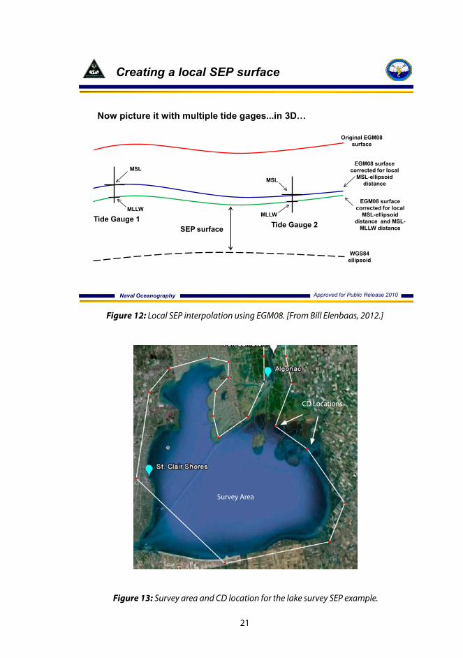
3.3 Interpolate Between SEP Locations with a Geoid ModelIt is a relatively simple procedure to use an existing geoid model to help interpolate be-tween established SEP locations. One can think of the process as shifting and warping a geoid model to fit established SEP sites (see Figure 12).

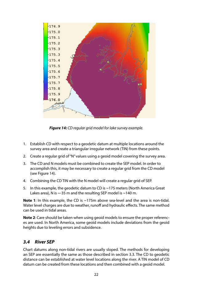
For example; In the case of a lake survey (see Figure 13):

21

Figure 12: Local SEP interpolation using EGM08. [From Bill Elenbaas, 2012.]

Naval Oceanography Approved for Public Release 2010

Original EGM08 surface

WGS84 ellipsoid

Tide Gauge 2

MSL

MLLWTide Gauge 1

MSL

MLLW

EGM08 surface corrected for local

MSL-ellipsoid distance

EGM08 surface corrected for local

MSL-ellipsoid distance and MSL-

MLLW distance

Now picture it with multiple tide gages...in 3D…

SEP surface

Creating a local SEP surface

Figure 13: Survey area and CD location for the lake survey SEP example.

Survey Area

CD Locations

22

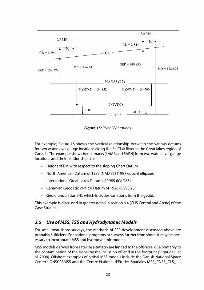
Figure 14: CD regular grid model for lake survey example.

1. Establish CD with respect to a geodetic datum at multiple locations around the survey area and create a triangular irregular network (TIN) from these points.

2. Create a regular grid of “N” values using a geoid model covering the survey area.

3. The CD and N models must be combined to create the SEP model. In order to accomplish this, it may be necessary to create a regular grid from the CD model (see Figure 14).

4. Combining the CD TIN with the N model will create a regular grid of SEP.

5. In this example, the geodetic datum to CD is ~175 meters (North America Great Lakes area), N is ~-35 m and the resulting SEP model is ~140 m.

Note 1: In this example, the CD is ~175m above sea-level and the area is non-tidal. Water level charges are due to weather, runoff and hydraulic effects. The same method can be used in tidal areas.

Note 2: Care should be taken when using geoid models to ensure the proper referenc-es are used. In North America, some geoid models include deviations from the geoid heights due to leveling errors and subsidence.

3.4 River SEPChart datums along non-tidal rivers are usually sloped. The methods for developing an SEP are essentially the same as those described in section 3.3. The CD to geodetic distance can be established at water level locations along the river. A TIN model of CD datum can be created from these locations and then combined with a geoid model.

23

LAMB

IGLD85

CD

NAD83 (97)

SARN

SEP = 139.778

N (NTv2) = -34.852

CD = 1.89

SEP = 140.830 Pub = 178.194

N (NTv2) = -34.790

CD = 2.544

CGVD28

Pub = 176.54

-0.02 -0.03

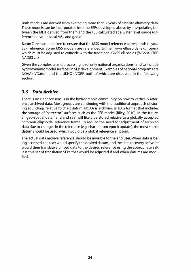
Figure 15: River SEP stations.

For example; Figure 15 shows the vertical relationship between the various datums for two water level gauge locations along the St. Clair River in the Great lakes region of Canada. The example shows benchmarks (LAMB and SARN) from two water level gauge locations and their relationships to:

– Height of BM with respect to the sloping Chart Datum

– North American Datum of 1983 (NAD 83) (1997 epoch) ellipsoid

– International Great Lakes Datum of 1985 (IGLD85)

– Canadian Geodetic Vertical Datum of 1928 (CGVD28)

– Geoid undulation (N), which includes variations from the geoid.

This example is discussed in greater detail in section 6.4 (CHS Central and Arctic) of the Case Studies.

3.5 Use of MSS, TSS and Hydrodynamic ModelsFor small near shore surveys, the methods of SEP development discussed above are probably sufficient. For national programs or surveys further from shore, it may be nec-essary to incorporate MSS and hydrodynamic models.

MSS models derived from satellite altimetry are limited to the offshore, due primarily to the contamination of the signal by the inclusion of land in the footprint (Vignudelli et al, 2008). Offshore examples of global MSS models include the Danish National Space Center’s DNSC08MSS and the Centre National d’Etudes Spatiales MSS_CNES_CLS_11.

24

Both models are derived from averaging more than 7 years of satellite altimetry data. These models can be incorporated into the SEPs developed above by interpolating be-tween the MDT derived from them and the TSS calculated at a water level gauge (dif-ference between local MSL and geoid).

Note: Care must be taken to ensure that the MSS model reference corresponds to your SEP reference. Some MSS models are referenced to their own ellipsoids (e.g. Topex), which must be adjusted to coincide with the traditional GNSS ellipsoids (WGS84, ITRF, NAD83 …)

Given the complexity and processing load, only national organizations tend to include hydrodynamic model surfaces in SEP development. Examples of national programs are NOAA’s VDatum and the UKHO’s VORF, both of which are discussed in the following section.

3.6 Data ArchiveThere is no clear consensus in the hydrographic community on how to vertically refer-ence archived data. Most groups are continuing with the traditional approach of stor-ing soundings relative to chart datum. NOAA is archiving in BAG format that includes the storage of “corrector” surfaces such as the SEP model (Riley, 2010). In the future, all geo-spatial data (land and sea) will likely be stored relative to a globally accepted common ellipsoidal reference frame. To reduce the need for adjustment of archived data due to changes in the reference (e.g. chart datum epoch update), the most stable datum should be used, which would be a global reference ellipsoid.

The actual data archive reference should be invisible to the end user. When data is be-ing accessed, the user would specify the desired datum, and the data recovery software would then translate archived data to the desired reference using the appropriate SEP. It is this set of translation SEPs that would be adjusted if and when datums are modi-fied.

25

4 QUALITY ASSURANCE AND QUALITY CONTROL

Essential components to the effective use of ERS are quality assurance and quality con-trol. According to ISO 9000 2005:

“Quality Assurance: A set of activities intended to establish confidence that quality requirements will be met.”

“Quality Control: A set of activities intended to ensure that quality requirements are actually being met.”

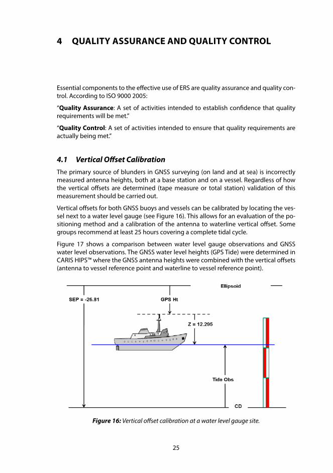
4.1 Vertical Offset CalibrationThe primary source of blunders in GNSS surveying (on land and at sea) is incorrectly measured antenna heights, both at a base station and on a vessel. Regardless of how the vertical offsets are determined (tape measure or total station) validation of this measurement should be carried out.

Vertical offsets for both GNSS buoys and vessels can be calibrated by locating the ves-sel next to a water level gauge (see Figure 16). This allows for an evaluation of the po-sitioning method and a calibration of the antenna to waterline vertical offset. Some groups recommend at least 25 hours covering a complete tidal cycle.

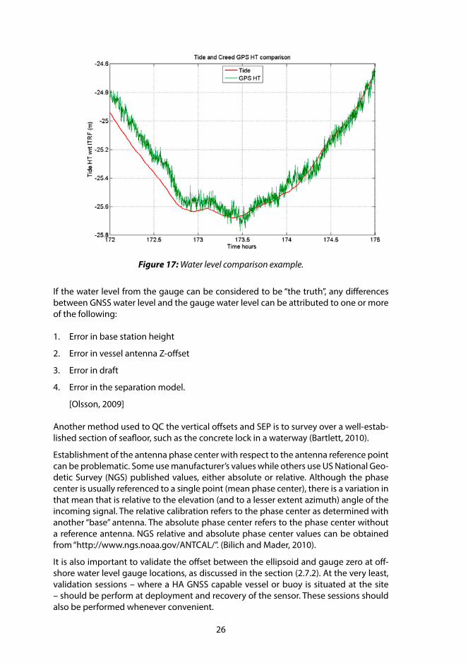
Figure 17 shows a comparison between water level gauge observations and GNSS water level observations. The GNSS water level heights (GPS Tide) were determined in CARIS HIPS™ where the GNSS antenna heights were combined with the vertical offsets (antenna to vessel reference point and waterline to vessel reference point).

Figure 16: Vertical offset calibration at a water level gauge site.

26

Figure 17: Water level comparison example.

If the water level from the gauge can be considered to be “the truth”, any differences between GNSS water level and the gauge water level can be attributed to one or more of the following:

1. Error in base station height

2. Error in vessel antenna Z-offset

3. Error in draft

4. Error in the separation model.

[Olsson, 2009]

Another method used to QC the vertical offsets and SEP is to survey over a well-estab-lished section of seafloor, such as the concrete lock in a waterway (Bartlett, 2010).

Establishment of the antenna phase center with respect to the antenna reference point can be problematic. Some use manufacturer’s values while others use US National Geo-detic Survey (NGS) published values, either absolute or relative. Although the phase center is usually referenced to a single point (mean phase center), there is a variation in that mean that is relative to the elevation (and to a lesser extent azimuth) angle of the incoming signal. The relative calibration refers to the phase center as determined with another “base” antenna. The absolute phase center refers to the phase center without a reference antenna. NGS relative and absolute phase center values can be obtained from “http://www.ngs.noaa.gov/ANTCAL/”. (Bilich and Mader, 2010).

It is also important to validate the offset between the ellipsoid and gauge zero at off-shore water level gauge locations, as discussed in the section (2.7.2). At the very least, validation sessions – where a HA GNSS capable vessel or buoy is situated at the site – should be perform at deployment and recovery of the sensor. These sessions should also be performed whenever convenient.

27

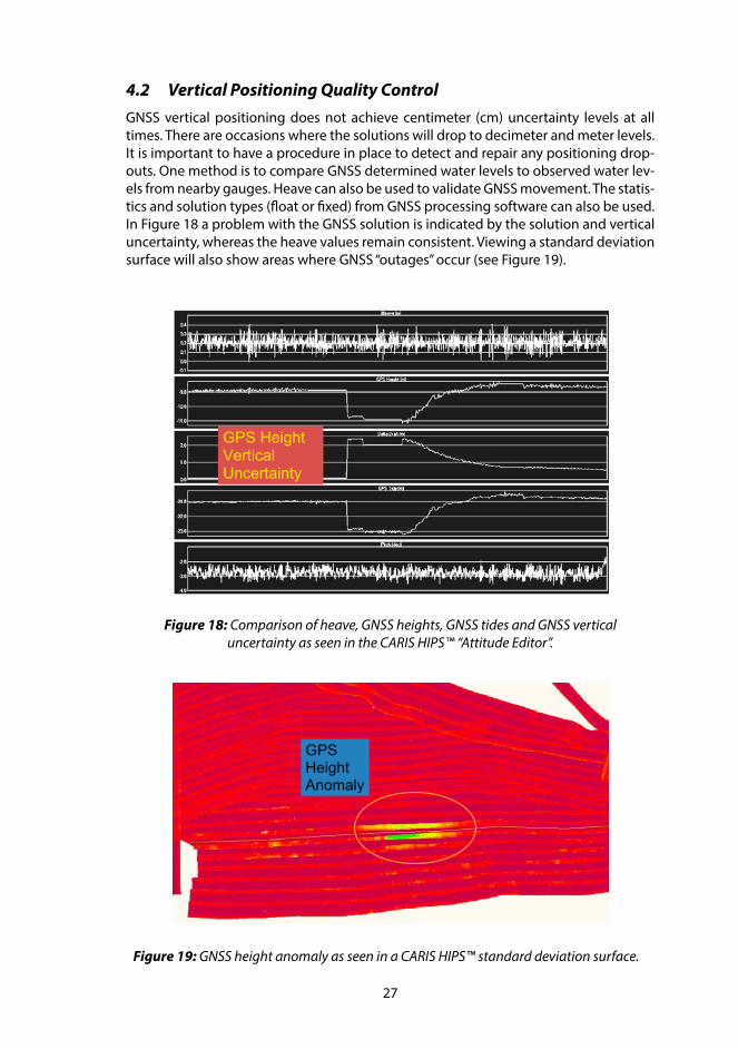
Figure 18: Comparison of heave, GNSS heights, GNSS tides and GNSS vertical uncertainty as seen in the CARIS HIPS™ “Attitude Editor”.

GPS Height Anomaly

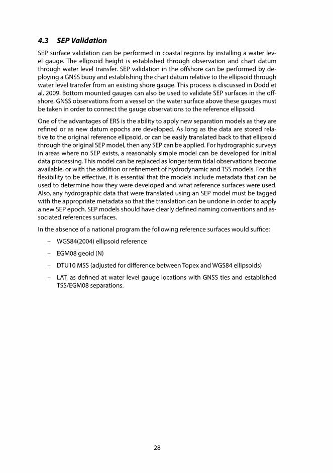
Figure 19: GNSS height anomaly as seen in a CARIS HIPS™ standard deviation surface.

4.2 Vertical Positioning Quality ControlGNSS vertical positioning does not achieve centimeter (cm) uncertainty levels at all times. There are occasions where the solutions will drop to decimeter and meter levels. It is important to have a procedure in place to detect and repair any positioning drop-outs. One method is to compare GNSS determined water levels to observed water lev-els from nearby gauges. Heave can also be used to validate GNSS movement. The statis-tics and solution types (float or fixed) from GNSS processing software can also be used. In Figure 18 a problem with the GNSS solution is indicated by the solution and vertical uncertainty, whereas the heave values remain consistent. Viewing a standard deviation surface will also show areas where GNSS “outages” occur (see Figure 19).

28

4.3 SEP ValidationSEP surface validation can be performed in coastal regions by installing a water lev-el gauge. The ellipsoid height is established through observation and chart datum through water level transfer. SEP validation in the offshore can be performed by de-ploying a GNSS buoy and establishing the chart datum relative to the ellipsoid through water level transfer from an existing shore gauge. This process is discussed in Dodd et al, 2009. Bottom mounted gauges can also be used to validate SEP surfaces in the off-shore. GNSS observations from a vessel on the water surface above these gauges must be taken in order to connect the gauge observations to the reference ellipsoid.

One of the advantages of ERS is the ability to apply new separation models as they are refined or as new datum epochs are developed. As long as the data are stored rela-tive to the original reference ellipsoid, or can be easily translated back to that ellipsoid through the original SEP model, then any SEP can be applied. For hydrographic surveys in areas where no SEP exists, a reasonably simple model can be developed for initial data processing. This model can be replaced as longer term tidal observations become available, or with the addition or refinement of hydrodynamic and TSS models. For this flexibility to be effective, it is essential that the models include metadata that can be used to determine how they were developed and what reference surfaces were used. Also, any hydrographic data that were translated using an SEP model must be tagged with the appropriate metadata so that the translation can be undone in order to apply a new SEP epoch. SEP models should have clearly defined naming conventions and as-sociated references surfaces.

In the absence of a national program the following reference surfaces would suffice:

– WGS84(2004) ellipsoid reference

– EGM08 geoid (N)

– DTU10 MSS (adjusted for difference between Topex and WGS84 ellipsoids)

– LAT, as defined at water level gauge locations with GNSS ties and established TSS/EGM08 separations.

29

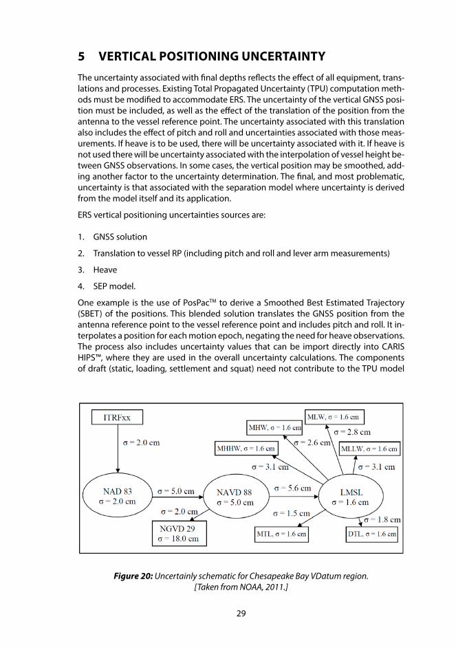
5 VERTICAL POSITIONING UNCERTAINTY

The uncertainty associated with final depths reflects the effect of all equipment, trans-lations and processes. Existing Total Propagated Uncertainty (TPU) computation meth-ods must be modified to accommodate ERS. The uncertainty of the vertical GNSS posi-tion must be included, as well as the effect of the translation of the position from the antenna to the vessel reference point. The uncertainty associated with this translation also includes the effect of pitch and roll and uncertainties associated with those meas-urements. If heave is to be used, there will be uncertainty associated with it. If heave is not used there will be uncertainty associated with the interpolation of vessel height be-tween GNSS observations. In some cases, the vertical position may be smoothed, add-ing another factor to the uncertainty determination. The final, and most problematic, uncertainty is that associated with the separation model where uncertainty is derived from the model itself and its application.

ERS vertical positioning uncertainties sources are:

1. GNSS solution

2. Translation to vessel RP (including pitch and roll and lever arm measurements)

3. Heave

4. SEP model.

One example is the use of PosPacTM to derive a Smoothed Best Estimated Trajectory (SBET) of the positions. This blended solution translates the GNSS position from the antenna reference point to the vessel reference point and includes pitch and roll. It in-terpolates a position for each motion epoch, negating the need for heave observations. The process also includes uncertainty values that can be import directly into CARIS HIPS™, where they are used in the overall uncertainty calculations. The components of draft (static, loading, settlement and squat) need not contribute to the TPU model

Figure 20: Uncertainly schematic for Chesapeake Bay VDatum region. [Taken from NOAA, 2011.]

30

as these offsets can be accounted for directly through ERS techniques. Due care is re-quired in the TPU modelling to properly switch on/off the component uncertainty con-tributions that directly contribute to reducing the observed depths.

Uncertainty in the SEP models includes a combination of uncertainties in all surfaces used to generate the model (ellipsoid, geoid, hydrodynamic, sea surface topography) as well as the translation between these surfaces.

In order to assign appropriate uncertainty to charted soundings it is necessary to in-clude the uncertainty associated with all aspects of the sounding derivation process, including those associated with the separation surfaces. Uncertainly associated with VDatum surfaces are discussed in the NOAA, 2011 document “Estimation of Vertical Uncertainties in VDatum.” Uncertainties are associated with each surface, as well as the uncertainty associated with the translation between surfaces. An example of uncer-tainties associated with VDatum in the Chesapeake Bay region is shown in Figure 20.

A single uncertainty value for a SEP is sufficient for a first estimate. However, a more realistic representation would be an uncertainty surface accompanying a SEP surface. Uncertainty at water level gauge locations will be at a minimum and increase with dis-tance from these locations. Uncertainty will also increase in areas of high tidal dynam-ics. Uncertainty in the SEP surface will also increase if hydrodynamic modeling and TSS modeling are not used. This subject requires more investigation and discussion.

31

6 CASE STUDIES

The following is a list of the case studies presented in this section:

1. Swedish Maritime Administration

2. CHS National Program

3. CHS Quebec

4. CHS Central and Arctic

5. NOAA VDatum

6. NOAA ERZT

7. VORF

8. BLAST

9. AusCoastVDT

10. NAVOCEANO.

6.1 Swedish Maritime AdministrationSource: Ulf Olsson personal communication (2009).

The Swedish Maritime Administration has been using ERS techniques since 2002. For high accuracy GNSS they use Network RTK and PPK. Traditional water level gauges are used in all surveys to validate GNSS heights and provide backup. Tides in Sweden have a small range; therefore they use MSL as the chart datum. A Swedish geoid model is used for ellipsoid to geoid, then local datum shifts to go from the geoid to chart datum (MSL). Grid maps of SEP offsets are used in both real-time and post processing applica-tions.

Traditional water level gauges are still installed for all surveys. This provides a contin-uous water level time series and a GNSS height verification tool. Vertical offsets are calibrated by laying the vessel near to the gauges and comparing the water levels. This calibration is performed at each water level gauge. The calibration is also conducted twice a day, once prior to and once at the end of each survey day.

PPK through PosPac™ is used for three dimensional positioning. A direct comparison between the PosPac™ results (adjusted to the waterline) and the water level gauges is made when the vessel is lying near the gauge (during calibration). The same compari-son cannot be made while the vessel is underway because of dynamic draft.

32

6.2 CHS National Project: Continuous Vertical Datums for Canadian Waters (2013)

Source: J. Bartlett1, M. Craymer2, B. de Lange Boom1 , K. Fadaie1, A. Godin1, D. Hains2, T. Herron1, P. MacAulay1, L. Maltais1, S. Nudds1, and C. Robin1,2, M. Véronneau2

Canada is developing national continuous vertical datum separation models (SEPs) between the GRS80 reference ellipsoid, tied to the NAD83(CSRS) geodetic reference frame, and Chart Datum (CD), the vertical reference of all hydrographic navigational charts. The project “Continuous Vertical Datum for Canadian Waters (CVDCW)” was initi-ated in 2009 and builds on previous localized work. First cut SEP solutions were com-pleted in 2013.

The CVDCW project is led by the Department of Fisheries and Oceans’ (DFO) Canadian Hydrographic Service (CHS) Hydrography Division with support from the Natural Re-sources Canada’s (NRCan) Canadian Geodetic Survey (CGS) and in collaboration with the Department of Fisheries and Oceans’ Ocean Science. Project implementation is through the CHS’s Tides, Currents and Water Levels (TCWL) group but the solutions are the results of synergy between the project’s multidisciplinary team of modelers, geod-esists, hydrographers, oceanographers and marine geodesists.

The primary aim of the CVDCW’s SEP solutions is to capture the spatial variability of CD with respect to the chosen NAD83 reference frame both along the coast between tidal stations and in the offshore. This is achieved through selective integration of both model and observational data sets. Sources include:

– Geoid (N, CGG2013): used to capture variation of the geoid with respect to the NAD83(CSRS) ellipsoid.

– Hydrodynamic oceanographic models: used to estimate variations in tidal re-gime, providing the initial separation estimate between lower low water large tide (LLWLT), or other datum, and MSL.

– Dynamic ocean topography (DOT) from ocean models (dynamically dependent mean water level (MSL) to geoid), used to connect MSL to the geoid.

– Satellite Altimetry: direct observations of MSL relative to the ellipsoid, used to validate the geoid, DOT and SEP.

– Tidal Stations: water level and GNSS observations, used to both validate and ad-just ocean model results. Station observations are also used to selectively force the final ideal model SEP solutions to locally honor currently adopted CD. Both water level and GNSS data and products used have been quality controlled and brought to the common SEP solution epoch to both account for ongoing land motion and sea level rise since data acquisition.

The main guiding principles used in the initial SEP development are:

1. To honor historic CD exactly at tidal stations where GNSS observations are available, and as closely as possible elsewhere.

1 Canadian Hydrographic Service, Department of Fisheries & Oceans

2 Canadian Geodetic Survey, Department of Natural Resources

33

2. To best capture the spatial variability of the datums with respect to the ellipsoid through integration of the best model and observational data sets available coupled with the most appropriate and expedient methods attainable. Methods to be developed with the flexibility to quickly and easily incorporate both improved model and observational data sets as they become available.

3. Methods to be packaged as a set of easily transportable tools running on the commonly used numerical computing environment ‘Matlab’ by MathWorks. Modularity and flexibility to be built into the toolset for universal geographical applicability to any region possessing the necessary input data sets and to accommodate

– the use of any ocean model dataset

– regional differences in geography, navigation and hydrographic practices

– rapid surface recalculation given future improvements in input data, modeled or observed

– continued improvement of methods.

4. To honor CD at individual water level stations the separation models are to be divided into two zones; the offshore, where the modeled SEP is applied directly, and a coastal transition zone where the observed CD is progressively more closely honored as the coastline is approached.

6.3 CHS Quebec Case Study (2009)Source: A. Godin, D. Langelier, A. Biron, C. Comtois, F. Lavoie, and D. Lefaivre

CHS Quebec is responsible for the Quebec portion of the Saint Lawrence Seaway out into the Gulf of Saint Lawrence (see Figure 21). The Quebec region is divided into two sections; channel and offshore. The channel group is responsible for surveying critical channel areas that are dredged to maintain minimum depth. Their area of responsibil-ity stretches from just west of Montreal to just east of Quebec City. The offshore group is responsible for all other navigable waters. The Quebec region started looking into the use of high-accuracy GNSS heights for surveying in 1995 and the technology is now an integral part of their operations. The following subsections give an overview of their application of ERS.

6.3.1 Data acquisitionA series of permanent GNSS base stations have been established along the shores of the Saint Lawrence River to enable the use of Real-Time Kinematic (RTK) positioning in all areas monitored by the channel group. The system in use is Thales™ LRK (Long Range Kinematic). Hypack™ is used for real-time navigation and tidal estimation using the RTK solutions. An ellipsoid to chart datum separation (SEP) model is used by Hy-pack™ to reduce the GNSS heights to chart datum. Heave and dynamic draft (if availa-ble) are also removed to produce an instantaneous tidal estimate, with respect to chart datum. This GNSS derived tidal estimate is compared to a predicted estimate derived from hydrodynamic modeling for real-time tide validation. The development of the SEP and prediction models will be discussed later.

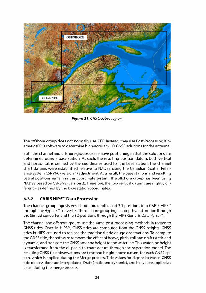
34

The offshore group does not normally use RTK. Instead, they use Post-Processing Kin-ematic (PPK) software to determine high-accuracy 3D GNSS solutions for the antenna.

Both the channel and offshore groups use relative positioning in that the solutions are determined using a base station. As such, the resulting position datum, both vertical and horizontal, is defined by the coordinates used for the base station. The channel chart datums were established relative to NAD83 using the Canadian Spatial Refer-ence System CSRS’96 (version 1) adjustment. As a result, the base stations and resulting vessel positions remain in this coordinate system. The offshore group has been using NAD83 based on CSRS’98 (version 2). Therefore, the two vertical datums are slightly dif-ferent – as defined by the base station coordinates.

6.3.2 CARIS HIPS™ Data ProcessingThe channel group ingests vessel motion, depths and 3D positions into CARIS HIPS™ through the Hypack™ converter. The offshore group ingests depths and motion through the Simrad converter and the 3D positions through the HIPS Generic Data Parser™.

The channel and offshore groups use the same post-processing methods in regard to GNSS tides. Once in HIPS™, GNSS tides are computed from the GNSS heights. GNSS tides in HIPS are used to replace the traditional tide gauge observations. To compute the GNSS tide, the software removes the effect of heave, pitch, roll and draft (static and dynamic) and transfers the GNSS antenna height to the waterline. This waterline height is transformed from the ellipsoid to chart datum through the separation model. The resulting GNSS tide observations are time and height above datum, for each GNSS ep-och, which is applied during the Merge process. Tide values for depths between GNSS tide observations are interpolated. Draft (static and dynamic), and heave are applied as usual during the merge process.

Figure 21: CHS Quebec region.

35

Once the GNSS tide has been computed, it is validated and smoothed in the attitude editor. Here it can be viewed with the GNSS height, heave, pitch, roll, and traditional tide (if available). A smoothing algorithm can be applied to the GNSS tide to remove any residual noise. The result is an actual tidal record that is applied to the soundings during the merge process; applying draft, heave, pitch and roll as usual.

6.3.3 Ellipsoid/Chart Datum Separation ModelsTwo separation models were used; one for the channel area and the other for the off-shore area. The channel model was based on the separation relative to the NAD83, CSRS96 (V1) ellipsoid, as per the GNSS reference stations. The separation between chart datum and the ellipsoid was determined through GNSS observations at each of the primary tide gauges and at intermediate tide staffs. Chart datum of the primary gauges was determined through long observations. Chart datum at each of the intermediate tide staffs was determined through linear interpolation, with respect to the Canadian Geodetic Vertical Datum (CGVD28), between primary tide gauges. The channel separa-tion model was created using Kriging, where the separation at the tide gauges and tide staff locations were considered to be correct; therefore fixed in the interpolation. No attempt was made to incorporate hydrodynamic modeling into the separation model. Extensive validation procedures were carried out to ensure the compatibility of GNSS derived tides and tradition observed tides, including static tests where vessels sat near to gauges and dynamic tests where vessels transited between, and by, primary tide gauges.

Both the offshore and channel SEP models were binary grid maps known as “BIN” files. The format was developed by the US National Geodetic Survey for the geoid/ellipsoid undulation models. The first channel version had a 6 arc-second grid and the current version has a 30 arc-second grid.

The software used to create the SEP maps was developed specifically for the channel area. It only accepted data with horizontal grid coordinates referenced to UTM Z18. Once the Kriging process was completed, the resulting SEP grid was transformed to geographic coordinates and then converted to the “BIN” format. The offshore area SEP maps, covered by UTM Z19 and Z20, had distortions resulting from the incompatible UTM zones. The software was no longer supported; therefore, updates or modifications were not possible. As a result, new SEP models are being developed. The new proce-dure still uses Kriging, but all processes can be performed on geographic coordinates.

Currently, the offshore model uses Kriging to interpolate between shore stations where the datum to ellipsoid is known. Consideration is being given to the incorporation of hydrodynamic models to help densify the network away from the shore stations. In-situ GPS tide gauges are also being considered to connect the hydrodynamic model to the ellipse.

6.3.4 Channel Validation Model (SPINE)While conducting hydrographic surveys in the channel region, operators can validate their GNSS tidal estimates in real-time. The GPS tides are estimated by Hypack using the RTK heights and the SEP model. The SPINE hydrodynamic model is used for a com-parison. This model is based on water level predictions from a hydrodynamic model combined with real-time tide gauge observations. The model produces water level es-timates at discrete locations (nodes) along the centerline of the river between Montreal

36

and Quebec City. At each location, the model predicts water level for a given time. The CHS hydrographers retrieve one day’s worth of predictions for each node, at 7.5 minute increments. These estimates are adjusted by real-time tide gauge observations, which are then interpolated for the location of the vessel. The resulting water level height is compared to the GPS derived height, in real-time, for validation.

6.4 CHS Central and ArcticSource: David Dodd, Jason Bartlett and Scott Youngblood

The CHS Central and Arctic region conducts hydrographic surveys in the Great Lakes and connecting waterways. In 2010 several surveys were conducted using ERS. The following outlines the procedure used for several ERS on the Saint Clair River between Lake St Clair and Lake Huron.

Post-processed kinematic (PPK) positioning with PosPac™ was used for three dimensional positioning of the vessels. GNSS base station coordinates were determined by submitting the daily observations to Natural Resources Canada (NRCan) Precise Point Positioning (PPP) online service. The separation (SEP) was developed from published information and validated by GNSS observation on benchmarks near permanent water level gauge sites. The vessel offsets were calibrated by docking near a water level gauge for a period of time (several hours) and comparing the GNSS derived water level to the gauge derived water level. The “GPS Tide” function in CARIS HIPS™ was used to apply the SEP. To validate the ERS processes water levels were also determined in HIPS™ using gauge observations. Both determinations of the water level (GNSS and traditional water level) were exported from HIPS™ and compared.

The following are more detailed descriptions of the vertical datums and SEP development.

6.4.1 Vertical DatumsTwo vertical datums are used in the Great Lakes region; CGVD28 (Canadian Vertical Da-tum of 1928) and IGLD85 (International Great Lakes Datum of 1985). Chart Datum is ref-erenced to IGLD85. The separation between IGLD85 and CGVD28 is published for perma-nent water level gauge locations, where chart datum has also been established. The el-lipsoid (NAD 83) to geoid (CGVD28) is established through the Natural Resources Canada (NRCan) NTv2 model.

During hydrographic surveys, vertical control is verified at permanent water level gauge locations through static GNSS observations (three hour sessions). The SEP translates from NAD83 > CGVD28 > IGLD85 > CD. The SEP for a water level benchmark (BM) is established through:

– BM height relative to CD

– BM height relative to IGLD85

– CGVD28-to-IGLD85 separation

– CGVD28 to NAD83 geoid/ellipsoid separation (N) from NRCan’s GPS-Hv2 NTv2 model.

– SEP (NAD83) = IGLD85 – CD + CGVD28-to-IGLD85 + N.

An example of the vertical datums at two St Clair River benchmarks is shown in Figure 22.

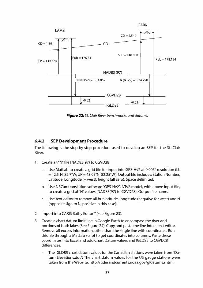
37

6.4.2 SEP Development ProcedureThe following is the step-by-step procedure used to develop an SEP for the St. Clair River.

1. Create an “N” file [NAD83(97) to CGVD28]

a. Use MatLab to create a grid file for input into GPS-Hv2 at 0.005° resolution (LL = 42.5°N, 82.7°W; UR = 43.05°N, 82.25°W). Output file includes: Station Number, Latitude, Longitude (+ west), height (all zero). Space delimited.

b. Use NRCan translation software “GPS-Hv2”, NTv2 model, with above input file, to create a grid of “N” values [NAD83(97) to CGVD28]. Output file name.

c. Use text editor to remove all but latitude, longitude (negative for west) and N (opposite sign to N, positive in this case).

2. Import into CARIS Bathy Editor™ (see Figure 23).

3. Create a chart datum limit line in Google Earth to encompass the river and portions of both lakes (See Figure 24). Copy and paste the line into a text editor. Remove all excess information, other than the single line with coordinates. Run this file through a MatLab script to get coordinates into columns. Paste these coordinates into Excel and add Chart Datum values and IGLD85 to CGVD28 differences.

– The IGLD85 chart datum values for the Canadian stations were taken from “Da-tum Elevations.doc”. The chart datum values for the US gauge stations were taken from the Website: http://tidesandcurrents.noaa.gov/gldatums.shtml.

Figure 22: St. Clair River benchmarks and datums.

LAMB

IGLD85

CD

NAD83 (97)

SARN

SEP = 139.778

N (NTv2) = -34.852

CD = 1.89

SEP = 140.830 Pub = 178.194

N (NTv2) = -34.790

CD = 2.544

CGVD28

Pub = 176.54

-0.02 -0.03

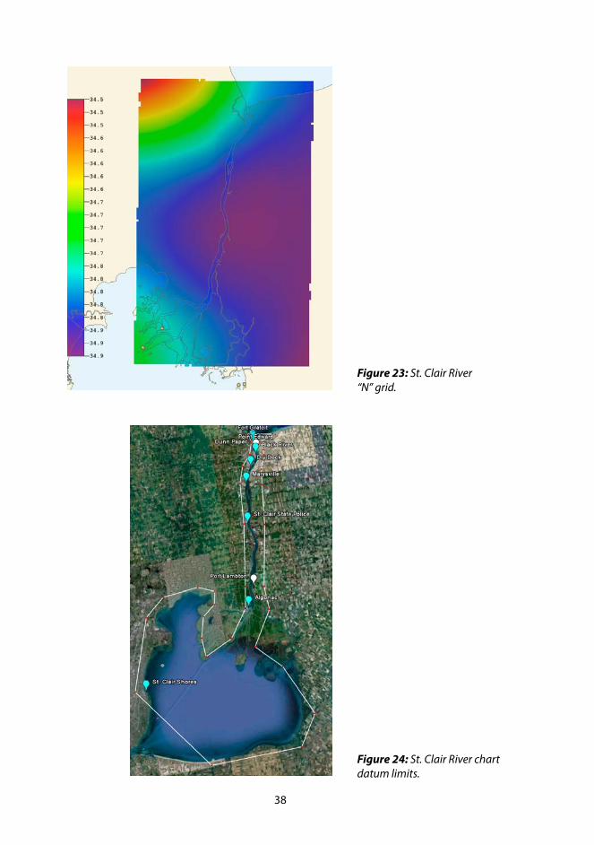
38

Figure 23: St. Clair River “N” grid.

Figure 24: St. Clair River chart datum limits.

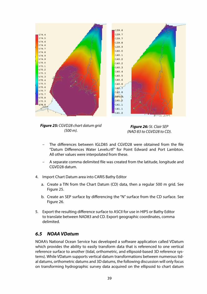
39

– The differences between IGLD85 and CGVD28 were obtained from the file “ Datum Differences Water Levels.rtf” for Point Edward and Port Lambton. All other values were interpolated from these.

– A separate comma delimited file was created from the latitude, longitude and CGVD28 datum.

4. Import Chart Datum area into CARIS Bathy Editor

a. Create a TIN from the Chart Datum (CD) data, then a regular 500 m grid. See Figure 25.

b. Create an SEP surface by differencing the “N” surface from the CD surface. See Figure 26.

5. Export the resulting difference surface to ASCII for use in HIPS or Bathy Editor to translate between NAD83 and CD. Export geographic coordinates, comma delimited.

6.5 NOAA VDatumNOAA’s National Ocean Service has developed a software application called VDatum which provides the ability to easily transform data that is referenced to one vertical reference surface to another (tidal, orthometric, and ellipsoid-based 3D reference sys-tems). While VDatum supports vertical datum transformations between numerous tid-al datums, orthometric datums and 3D datums, the following discussion will only focus on transforming hydrographic survey data acquired on the ellipsoid to chart datum

Figure 25: CGVD28 chart datum grid (500 m).

Figure 26: St. Clair SEP (NAD 83 to CGVD28 to CD).

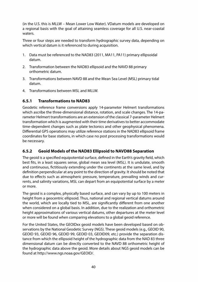
40

(in the U.S. this is MLLW – Mean Lower Low Water). VDatum models are developed on a regional basis with the goal of attaining seamless coverage for all U.S. near-coastal waters.

Three or four steps are needed to transform hydrographic survey data, depending on which vertical datum is it referenced to during acquisition.

1. Data must be referenced to the NAD83 (2011, MA11, PA11) primary ellipsoidal datum.

2. Transformation between the NAD83 ellipsoid and the NAVD 88 primary orthometric datum.

3. Transformations between NAVD 88 and the Mean Sea Level (MSL) primary tidal datum.

4. Transformations between MSL and MLLW.

6.5.1 Transformations to NAD83Geodetic reference frame conversions apply 14-parameter Helmert transformations which ascribe the three-dimensional distance, rotation, and scale changes. The 14-pa-rameter Helmert transformations are an extension of the classical 7-parameter Helmert transformation which is augmented with their time derivatives to better accommodate time-dependent changes such as plate tectonics and other geophysical phenomena. Differential GPS operations may utilize reference stations in the NAD83 ellipsoid frame coordinates for base stations, in which case no post processing transformations would be necessary.

6.5.2 Geoid Models of the NAD83 Ellipsoid to NAVD88 SeparationThe geoid is a specified equipotential surface, defined in the Earth’s gravity field, which best fits, in a least squares sense, global mean sea level (MSL). It is undulate, smooth and continuous, fictitiously extending under the continents at the same level, and by definition perpendicular at any point to the direction of gravity. It should be noted that due to effects such as atmospheric pressure, temperature, prevailing winds and cur-rents, and salinity variations, MSL can depart from an equipotential surface by a meter or more.

The geoid is a complex, physically based surface, and can vary by up to 100 meters in height from a geocentric ellipsoid. Thus, national and regional vertical datums around the world, which are locally tied to MSL, are significantly different from one another when considered on a global basis. In addition, due to the realization and orthometric height approximations of various vertical datums, other departures at the meter level or more will be found when comparing elevations to a global geoid reference.

For the United States, the GEOIDxx geoid models have been developed based on ob-servations by the National Geodetic Survey (NGS). These geoid models (e.g., GEOID 90, GEOID 93, GEOID 96, GEOID 99, GEOID 03, GEOID09, etc.) provide the separation dis-tance from which the ellipsoid height of the hydrographic data from the NAD 83 three dimensional datum can be directly converted to the NAVD 88 orthometric height of the hydrographic data above the geoid. More details about NGS geoid models can be found at http://www.ngs.noaa.gov/GEOID/.

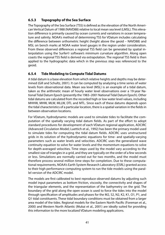
41

6.5.3 Topography of the Sea SurfaceThe Topography of the Sea Surface (TSS) is defined as the elevation of the North Ameri-can Vertical Datum of 1988 (NAVD88) relative to local mean sea level (LMSL). This eleva-tion difference is primarily caused by ocean currents and variations in ocean tempera-ture and salinity. NOAA’s method of determining TSS for VDatum includes calculating the difference between orthometric height (height above the geoid – NAVD88) and MSL on bench marks at NOAA water level gauges in the region under consideration. From these observed differences a regional TSS field can be generated by spatial in-terpolation using the Surfer© software’s minimum curvature algorithm. Along open coasts the regional TSS field is derived via extrapolation. The regional TSS field is then applied to the hydrographic data which in the previous step was referenced to the geoid.

6.5.4 Tide Modeling to Compute Tidal DatumsA tidal datum is a base elevation from which relative heights and depths may be deter-mined (Gill and Schultz, 2001). It can be computed by analyzing a time series of water levels from observational data. Mean sea level (MSL) is an example of a tidal datum, taken as the arithmetic mean of hourly water level observations over a 19-year Na-tional Tidal Datum Epoch (presently the 1983–2001 National Tidal Datum Epoch). Other tidal datums are calculated from the recorded high or low water level values, including MHHW, MHW, MLW, MLLW, DTL and MTL. Since each of these datums depends upon the tidal characteristics of a particular location, there is a spatial variation in the fields in between observation locations.

For VDatum, hydrodynamic models are used to simulate tides to facilitate the com-putation of the spatially varying tidal datum fields. As part of the effort to adopt standard procedures for development of each VDatum regional application, ADCIRC (Advanced Circulation Model; Luettich et al., 1992) has been the primary model used to simulate tides for computing the tidal datum fields. ADCIRC uses unstructured grids in its solution of the hydrodynamic equations for time- and spatially-varying parameters such as water levels and velocities. ADCIRC uses the generalized wave continuity equation to solve for water levels and the momentum equations to solve for depth-averaged velocities. Time steps used by the model vary according to the smallest size of triangles in a grid, and they are typically on the order of a few seconds or less. Simulations are normally carried out for two months, and the model must therefore process several million time steps for completion. Due to these computa-tional requirements, NOAA’s Earth System Research Laboratory (ESRL) granted access to their high performance computing system to run the tide models using the paral-lel version of the ADCIRC model.

The models are first calibrated to best reproduce observed datums by adjusting such model input parameters as bottom friction, viscosity, the connectivity and shapes of the triangular elements, and the representation of the bathymetry on the grid. The boundary of the grid along the open ocean is used to force the tides into the model through specification of amplitudes and phases for the M2, S2, N2, K2, K1, O1, P1, and Q1 tidal constituents. These tidal boundary conditions must be obtained from a larger area model of the tides. Regional models for the Eastern North Pacific (Foreman et al., 2000) and Western North Atlantic (Mukai et al., 2001) are ideally suited for providing this information to the more localized VDatum modeling applications.

42

After the model parameters have been calibrated, simulations are made to adjust the bathymetry to be vertically referenced to MSL. As bathymetry in the U.S. is referenced to MLLW, an initial guess of the MSL to MLLW difference is made to correct the bathym-etry for a tide simulation. After that initial simulation is complete, the model output is used to compute new MLLW-MSL differences that are then used as a new correction to the bathymetry. The process is repeated until the computed corrections do not change from one simulation to the next.

A final hydrodynamic model simulation with the calibrated parameters and corrected bathymetry is then made, and time series of the modeled water levels are analyzed at each node in the grid to compute spatially varying tidal datum fields. The modeled datums at NOAA’s NWLON (National Water Level Observation Network) stations are compared with those derived from observations. Model-data differences are spatially interpolated using TCARI (Hess, 2002; Tidal Constituent And Residual Interpolation), a software tool based on solution of Laplace’s equation using the shoreline as a bounda-ry. Most of the model-data differences are less than 10 cm for all of the VDatum regions, though there are some instances where the errors may be slightly larger. The values of these differences are identified in the VDatum reports for each of the regional pro-jects. These interpolated differences are used as correction fields to the modeled tidal datums, such that the corrected modeled datums will now match exactly at locations where observations are available.

VDatum incorporates the corrected version of the modeled tidal datums through the use of a marine grid. This is a regularly spaced set of data points, onto which the cor-rected model results are interpolated. Using the high resolution shoreline data, each marine grid point is evaluated as to whether it falls inside (land) or outside (water) this shoreline. A small buffer is also taken into account, such that marine grid points that fall just slightly on the land (within 0.1 nautical miles) may still be assigned a tidal datum value. The final marine grid of tidal datum fields is provided as input to the VDatum software. Then user-supplied reference datum, elevation, and longitude/latitude pair data may be entered into VDatum, which will interpolate the desired tidal datum from the marine grid. VDatum is then used to transform the hydrographic data from the pre-vious step which was referenced to MSL to Chart Datum (MLLW in the U.S.).

6.6 NOAA Ellipsoidally Referenced Zoned Tides & GNSS Water Level Buoys

VDatum models are currently available for all near shore waters of the U.S. except Alas-ka and Hawaii where additional gravity and water level data are needed. Completion of VDatum models in those states will not be completed until after 2020. However, be-cause there is a significant improvement in the quality and consistency of hydrographic data acquired relative to the ellipsoid, NOAA has begun developing a procedure to measure the water level datum relative to the ellipsoid (Rice and Riley, 2011) thereby developing a SEP model during data acquisition.

Traditional hydrographic water level modeling methods use some form of “zoning” (constant offset, discrete zones, or continuous surface) to define areas of similar water level regimes. The process described here uses ship-based measurements relative to the ellipsoid and tidal zoning to create discrete SEP “zones”. Hence the name adopted for this process is ellipsoidally referenced zoned tides, or ERZT.

43

Conventional hydrographic surveying techniques apply corrections for tides, static draft and vessel dynamics directly to sounding data. Tide corrections are typically de-termined from the above mentioned tidal zoning. Static draft is determined when the vessel is at rest and monitored for change during the survey due to vessel loading. Ves-sel dynamics include heave due to wave action and dynamic draft which reflect chang-es due to a vessel’s movement through the water (changes in trim are called squat and changes in height relative to the water’s surface at rest is called settlement). For ERS surveys these corrections are not applied to the sounding data. Rather, the sounding data (after sound velocity corrections have been made) is directly referenced to the el-lipsoid creating a very consistent coherent surface.

Developing the SEP model for transforming this smooth ellipsoidally referenced sea floor surface to chart datum using ERZT can be done in three steps:

1. During data acquisition the vessel’s GPS antenna height (as well as the ship’s Reference Point (RP) and other offset points on the vessel) above/below the ellipsoid is continually recorded resulting in a vessel ellipsoid height time series. This time series reflects vertical changes due to the above mentioned tides, changes in static draft and vessel dynamics. By removing the static draft changes and the effects of vessel dynamics, a time series can be created that reflects only vertical changes due to changes in water level (tides plus weather induced changes). These are removed just as they are in conventional hydrography. Changes in draft, while generally minor, are corrected for and accurate heave is extracted from the vessel’s inertial navigation system data. Low frequency motion due to dynamic draft must be modeled. (Note: Ideally this should be done relative to speed through the water but has historically been calculated in NOAA relative to speed over ground. In areas of little or no current, the error induced from this is negligible but may induce an error of up to one or two feet in shallow areas with high currents.) The result of applying these corrections is a time series of the quiescent in situ water level relative to the ellipsoid.

2. Corrections for variations in water level for conventional hydrographic surveys use zones, each of which has a specific phase offset and amplitude or range ratio from the water level at a control gauge. Therefore, for every zone and for every point in each zone, the water level relative to the chart datum (MLLW for the U.S.) can be calculated. This water level relative to MLLW is then simply added to the water level relative to the ellipsoid (above) to yield a time series of in situ SEP.

3. This observed SEP time series can then be used to create a gridded surface by averaging over appropriately sized bins comparable to the governing tide zones and geoidal variations. The result is a SEP model of the survey area. A nominal regular bin size of one kilometer is a good starting point.

While the estimates associated with this process incorporate the somewhat imprecise vessel dynamic waterline and zoned/interpolated water level reducer model, averag-ing over a large number of repeated measurements forms a relatively smooth SEP sur-face of reduced uncertainty.

Conventional hydrographic surveys require time-delayed analysis of water level gauge data to produce final water leveling zoning using actual water level measurements from control water level gauges and any subordinate gauges required by the survey. This analysis results in final zoning which is often significantly different from prelimi-

44

nary zoning. In such cases the sounding data needs to be reprocessed, and quality con-trolled in the field. Using ERZT, rather than the sounding data being reprocessed, the SEP needs to be recalculated which may eventually take less effort and can take place away from the field unit.

Early comparisons between ERZT and VDatum SEPs have been quite favorable (mean difference near 1 centimeter with a standard deviation of 3–5 centimeters). As such, ERZT can likely be used to check/validate VDatum models where they exist. CARIS HIPS™ version 8.1.5+ includes an ERZT computation tool (ProcessCompute Separa-tion Model) that NOAA is using to conduct operational testing of the concept in 2014.

NOAA is also conducting operational tests of GPS water level buoys in 2014 in conjunc-tion with regular hydrographic survey work. The Office of Coast Survey (OCS) owns two GPS AXYS Technologies Inc. Hydrolevel™ GPS buoys. The OCS Hydrolevel™ buoys utilize PPK along with a tilt sensor. Deployment plans include an environmental assessment to decide on where best to position the GPS buoy system for a particular hydrographic survey project area, based upon available knowledge of the local tidal currents, sur-face waves, and bathymetry. The project planning process will also target the extent to which the data from the buoy is to be used. As with current and historical water level data, some data is directly used as observed water level, some data is only used in the generation of products (such as harmonic constituents and tidal datums), and some data is used to provide general information about the tidal characteristics of an area, including SEP formulation and verification.

6.7 United Kingdom Hydrographic Office VORFThe UKHO’s Vertical Offshore Reference Frame (VORF) is a collection of surfaces used to transform between various datums for the entire United Kingdom and Irish conti-nental shelves. Each surface is referenced to the WGS84 ellipsoid. Surfaces include HAT, MHWS, MSL, MLWS, LAT, Chart Datum and Ordinance Survey Datums. The standard surface grid resolution is 0.008°, with 0.003° resolution in complex tidal regimes and in rivers. (Howlett, 2009)

The OSGM05 gravity model was used to establish the geoid to WGS84 ellipsoid un-dulation (N). TSS, relative to the WSG84 ellipsoid, was established through water level gauge observations (near shore) and satellite altimetry (off shore). The connection be-tween MSL and LAT was achieved through observation at water level gauges and hy-drodynamic modeling (Adams et al, 2006).

Permanent and temporary water level gauges along the shoreline were used to estab-lish a link between the geoid, MSL, LAT and CD. Chart datums (CD) are local and often derived from short term observations and there is no consistent connection to LAT. The CD surfaces were developed by establishing deviations from LAT at know CD locations (Howlett, 2009). GNSS observations at selected gauges were used to establish a link to the WGS84 reference ellipsoid. The WGS84 ellipsoid, OSGM05 geoid model, satellite al-timetry model and hydrodynamic models were used to propagate the various surfaces into the offshore.

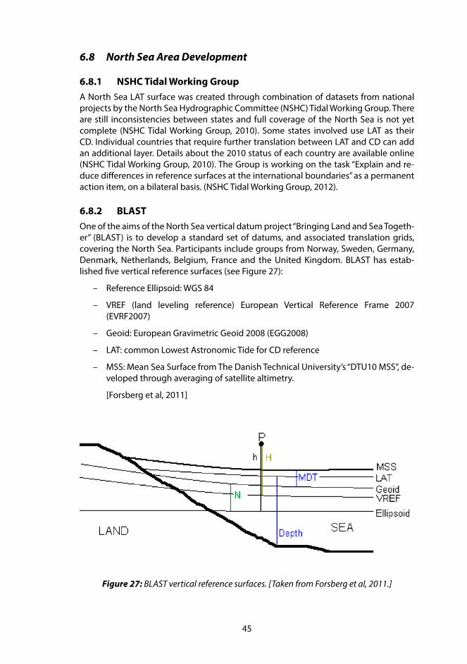
45

6.8 North Sea Area Development

6.8.1 NSHC Tidal Working GroupA North Sea LAT surface was created through combination of datasets from national projects by the North Sea Hydrographic Committee (NSHC) Tidal Working Group. There are still inconsistencies between states and full coverage of the North Sea is not yet complete (NSHC Tidal Working Group, 2010). Some states involved use LAT as their CD. Individual countries that require further translation between LAT and CD can add an additional layer. Details about the 2010 status of each country are available online (NSHC Tidal Working Group, 2010). The Group is working on the task “Explain and re-duce differences in reference surfaces at the international boundaries” as a permanent action item, on a bilateral basis. (NSHC Tidal Working Group, 2012).

6.8.2 BLASTOne of the aims of the North Sea vertical datum project “Bringing Land and Sea Togeth-er” (BLAST) is to develop a standard set of datums, and associated translation grids, covering the North Sea. Participants include groups from Norway, Sweden, Germany, Denmark, Netherlands, Belgium, France and the United Kingdom. BLAST has estab-lished five vertical reference surfaces (see Figure 27):

– Reference Ellipsoid: WGS 84

– VREF (land leveling reference) European Vertical Reference Frame 2007 (EVRF2007)

– Geoid: European Gravimetric Geoid 2008 (EGG2008)

– LAT: common Lowest Astronomic Tide for CD reference

– MSS: Mean Sea Surface from The Danish Technical University’s “DTU10 MSS”, de-veloped through averaging of satellite altimetry.

[Forsberg et al, 2011]

Figure 27: BLAST vertical reference surfaces. [Taken from Forsberg et al, 2011.]

46

The translations between surfaces are achieved through four basic grids:

1. EGG2008 geoid to ellipsoid separation (N).

2. Mean Dynamic Topography of the Sea (MDT or TSS) which is DTU10 MSS minus EGG2008, with checks at water level gauge locations. Translates from Geoid to MSL. DTU10 MDT is also corrected for a deviation from the DTU10 MSS ellipsoid (Topex) and EGG2008 ellipsoid (~0.90 m).

3. LAT surface, difference between LAT and MSS, translates from MSL to LAT.

4. EVRF-DIF surface that translates from EGG2008 to EVRF2007.

[Forsberg et al, 2011]

It is anticipated that VORF will be aligned with the BLAST vertical reference surfaces [Howlett, 2009].

6.8.3 Cooperation Between NSHC and BLASTThe Tidal Working Group has been in close contact with the BLAST project, aiming at directing the research activities and applying the results. At the end of the project, the Tidal Working Group concluded that “Thanks to BLAST, a consistent LAT reference sur-face is available for most of the area of interest of the NSHC. This surface is available through a preliminary software package that is not publicly available.” Also, the Group recommended that “Further efforts are necessary to create an LAT surface for the full area of interest of the NSHC. Also, further efforts are necessary to create public access to this LAT surface, in a user-friendly software package and/or by offering the data online. Only after completion of these two efforts, an LAT surface should be accepted by the NSHC as common and unique.”

6.9 AusCoastVDTAustralia has developed a tool (AusCoastVDT) for translating between a variety of el-lipsoid, geoid and tidal vertical datums. The translation grids cover all Australian coastal waters. More information can be found at:

http://www.crcsi.com.au/Research/Commissioned-Research/9-06-UDEM-for-CC/ sub-project-2

6.10 US Naval Oceanographic Office (NAVOCEANO)

6.10.1 NAVOCEANO with the Brazilian Directorate of Hydrography and Navigation (DNH)

Source: Aluizio M. Oliveira Jr, Elliot N. Arroyo-Suarez, Alexandre M. Ramos, Maria Fer-nanda R. Arentz,

This section describes the cooperative tests executed by both naval offices NAVOCEANO and DHN in order to evaluate the seabed mapping in an earth centered earth fixed (ECEF) geocentric reference frame. The field experimentation was performed in Guanabara Bay, Rio de Janeiro, from 06 to 17 July 2009. Data collection included GPS surveys at six tide

47

stations locations, hydrodynamic modeling, water level measurements, local datum computation using different software packages and ECEF bathymetric surveys. Data pro-cessing using both traditional method with local tide gauge measurements and ECEF method with tidal information extracted from GPS and hydrodynamic computations al-lowed a comparison of results. This joint survey allowed both institutions to validate ECEF survey techniques that can potentially be utilized in areas where in-situ data do not exist or are difficult to obtain. Also permitted that Brazilian Geoidal model MAPGEO2010 could be tested for ECEF surveys applications. [Oliveira et. al., 2010]

The following project summary was provided by Elliot Arroyo-Suarez in 2010.

Ellipsoidal Referenced Surveying is in transition, the primary depth reduction method is still through traditional water level observations and new methods used when tradi-tional method uncertainty is too high.

Real-time vertical positioning with NavCom™ Real Time Gipsy (RTG) service and raw GNSS navigation recorded (both NavCom™ & Trimble™). An automated post-process-ing PPP procedure was implemented using rapid orbits and clocks. The post processed PPP-derived trajectory (with 24 hours of latency) replaced RTG-derived trajectory, im-proving vertical uncertainty by almost a 100% (from ~ 35 cm to ~ 15 cm @ 95%).

During data acquisition, the SEP was built using EGM08 in waters deeper than 200 me-ters and EGM08 + Zo (MSL to CD) for waters less than 200 m. A hydrodynamic model was used to produce a time series and subsequent tidal constituents on each of the model nodes. Zo was determined on each of the nodes utilizing the traditional Range-Ratio method, or the modified Range-Ratio method, depending on the type of tide at designated primary tide stations.

Ellipsoid to water level separation (MHWL, MSL and MLLW) was determined using a combination of GNSS buoy (RTG, and PPP) and land-based GNSS levelling (if access to land was possible). A “residual” surface was produced from in-situ measurements (GNSS levelling and GNSS buoys) and EGM08. The residual surface derived by differenc-ing the in-situ ellipsoid height of MSL from EGM08. The final SEP was determined from:

SEP = EGM08 + Zo + Residual (See Figure 28)

All vertical vessel offsets were verified in port at water level gauge locations.

The “Zo” surface was produced from a hydrodynamic model, which was developed by first setting up the model domain with offshore boundaries, typically outside the conti-nental shelf. The model domain included soundings from Digital Nautical Charts (DNC). Each sounding constituted a node in the model, and the hydrodynamic equations were run on each node. The modeler also added friction parameter for the bottom and water surface.

Once the model domain was developed, forcing mechanisms, such as winds and boundary tidal constituents were established. The tidal constituents were obtained from global models such as FES (Finite Element Solution) which were derived from the analysis of satellite altimeter data.

The ADCIRC (ADvanced CIRCulation) model was run using the forcing mechanisms and boundary conditions. The model had some spin-up time (5 days) thus simulation was run to cover 35 days. The model produced a time-series of water level heights relative to MSL as well as tidal constituents for each node.

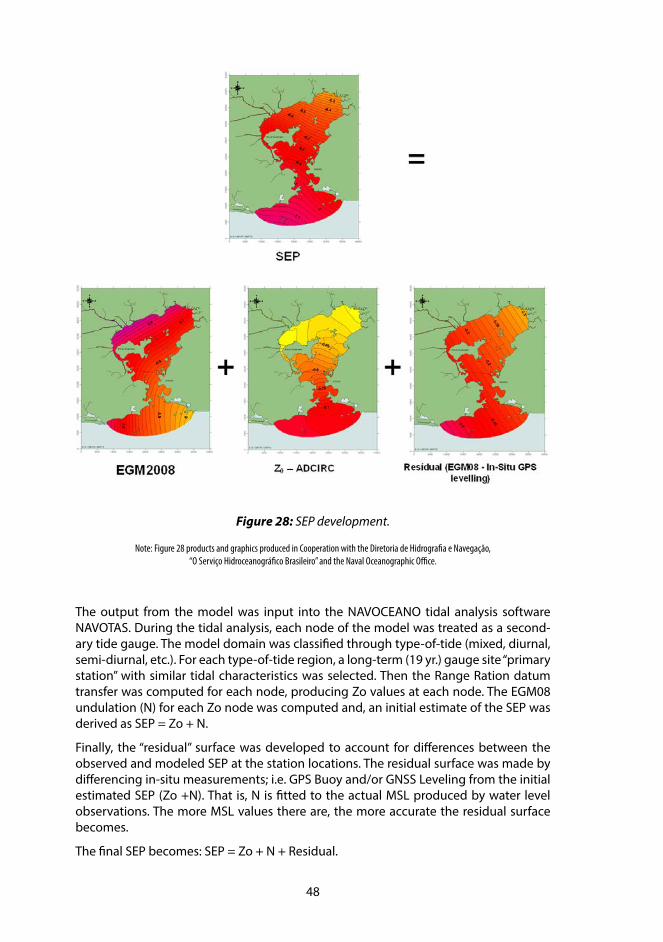
48

The output from the model was input into the NAVOCEANO tidal analysis software NAVOTAS. During the tidal analysis, each node of the model was treated as a second-ary tide gauge. The model domain was classified through type-of-tide (mixed, diurnal, semi-diurnal, etc.). For each type-of-tide region, a long-term (19 yr.) gauge site “primary station” with similar tidal characteristics was selected. Then the Range Ration datum transfer was computed for each node, producing Zo values at each node. The EGM08 undulation (N) for each Zo node was computed and, an initial estimate of the SEP was derived as SEP = Zo + N.

Finally, the “residual” surface was developed to account for differences between the observed and modeled SEP at the station locations. The residual surface was made by differencing in-situ measurements; i.e. GPS Buoy and/or GNSS Leveling from the initial estimated SEP (Zo +N). That is, N is fitted to the actual MSL produced by water level observations. The more MSL values there are, the more accurate the residual surface becomes.

The final SEP becomes: SEP = Zo + N + Residual.

Figure 28: SEP development.

Note: Figure 28 products and graphics produced in Cooperation with the Diretoria de Hidrografia e Navegação, “O Serviço Hidroceanográfico Brasileiro” and the Naval Oceanographic Office.

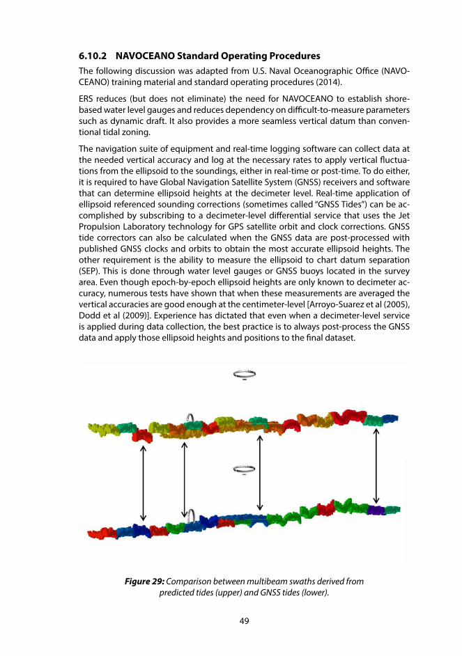
49

6.10.2 NAVOCEANO Standard Operating ProceduresThe following discussion was adapted from U.S. Naval Oceanographic Office (NAVO-CEANO) training material and standard operating procedures (2014).

ERS reduces (but does not eliminate) the need for NAVOCEANO to establish shore-based water level gauges and reduces dependency on difficult-to-measure parameters such as dynamic draft. It also provides a more seamless vertical datum than conven-tional tidal zoning.

The navigation suite of equipment and real-time logging software can collect data at the needed vertical accuracy and log at the necessary rates to apply vertical fluctua-tions from the ellipsoid to the soundings, either in real-time or post-time. To do either, it is required to have Global Navigation Satellite System (GNSS) receivers and software that can determine ellipsoid heights at the decimeter level. Real-time application of ellipsoid referenced sounding corrections (sometimes called “GNSS Tides”) can be ac-complished by subscribing to a decimeter-level differential service that uses the Jet Propulsion Laboratory technology for GPS satellite orbit and clock corrections. GNSS tide correctors can also be calculated when the GNSS data are post-processed with published GNSS clocks and orbits to obtain the most accurate ellipsoid heights. The other requirement is the ability to measure the ellipsoid to chart datum separation (SEP). This is done through water level gauges or GNSS buoys located in the survey area. Even though epoch-by-epoch ellipsoid heights are only known to decimeter ac-curacy, numerous tests have shown that when these measurements are averaged the vertical accuracies are good enough at the centimeter-level [Arroyo-Suarez et al (2005), Dodd et al (2009)]. Experience has dictated that even when a decimeter-level service is applied during data collection, the best practice is to always post-process the GNSS data and apply those ellipsoid heights and positions to the final dataset.

Figure 29: Comparison between multibeam swaths derived from predicted tides (upper) and GNSS tides (lower).

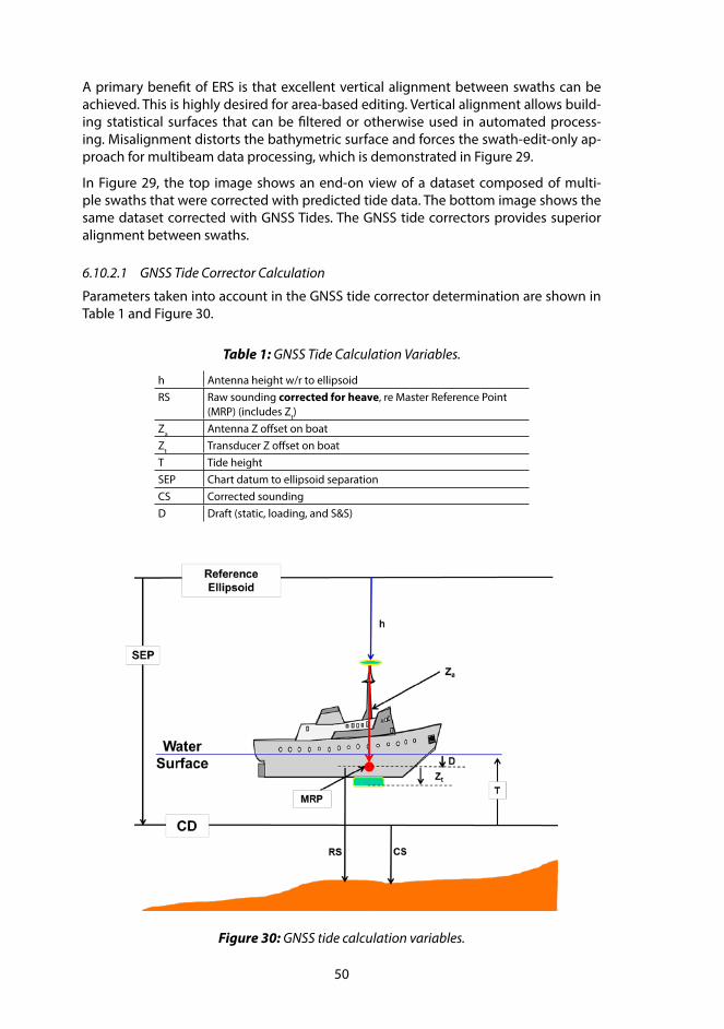
50

A primary benefit of ERS is that excellent vertical alignment between swaths can be achieved. This is highly desired for area-based editing. Vertical alignment allows build-ing statistical surfaces that can be filtered or otherwise used in automated process-ing. Misalignment distorts the bathymetric surface and forces the swath-edit-only ap-proach for multibeam data processing, which is demonstrated in Figure 29.

In Figure 29, the top image shows an end-on view of a dataset composed of multi-ple swaths that were corrected with predicted tide data. The bottom image shows the same dataset corrected with GNSS Tides. The GNSS tide correctors provides superior alignment between swaths.

6.10.2.1 GNSS Tide Corrector Calculation

Parameters taken into account in the GNSS tide corrector determination are shown in Table 1 and Figure 30.

Table 1: GNSS Tide Calculation Variables.

h Antenna height w/r to ellipsoidRS Raw sounding corrected for heave, re Master Reference Point

(MRP) (includes Zt)Za Antenna Z offset on boatZt Transducer Z offset on boatT Tide heightSEP Chart datum to ellipsoid separationCS Corrected sounding D Draft (static, loading, and S&S)

Figure 30: GNSS tide calculation variables.

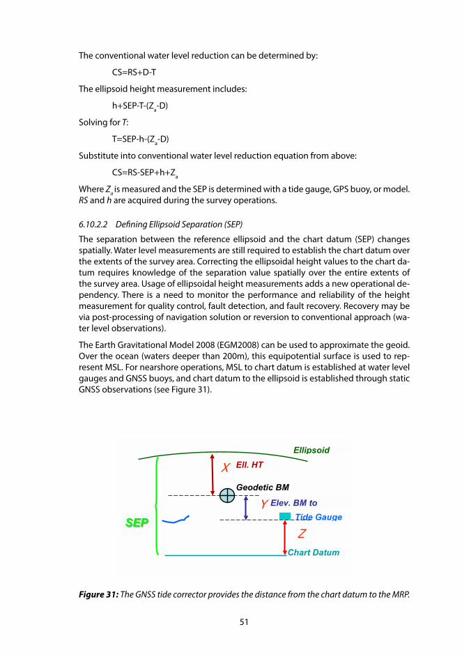
51

The conventional water level reduction can be determined by:

CS=RS+D-T

The ellipsoid height measurement includes:

h+SEP-T-(Za-D)

Solving for T:

T=SEP-h-(Za-D)

Substitute into conventional water level reduction equation from above:

CS=RS-SEP+h+Za

Where Za is measured and the SEP is determined with a tide gauge, GPS buoy, or model. RS and h are acquired during the survey operations.

6.10.2.2 Defining Ellipsoid Separation (SEP)

The separation between the reference ellipsoid and the chart datum (SEP) changes spatially. Water level measurements are still required to establish the chart datum over the extents of the survey area. Correcting the ellipsoidal height values to the chart da-tum requires knowledge of the separation value spatially over the entire extents of the survey area. Usage of ellipsoidal height measurements adds a new operational de-pendency. There is a need to monitor the performance and reliability of the height measurement for quality control, fault detection, and fault recovery. Recovery may be via post-processing of navigation solution or reversion to conventional approach (wa-ter level observations).

The Earth Gravitational Model 2008 (EGM2008) can be used to approximate the geoid. Over the ocean (waters deeper than 200m), this equipotential surface is used to rep-resent MSL. For nearshore operations, MSL to chart datum is established at water level gauges and GNSS buoys, and chart datum to the ellipsoid is established through static GNSS observations (see Figure 31).

Figure 31: The GNSS tide corrector provides the distance from the chart datum to the MRP.

Ellipsoid

Geodetic BM

Tide Gauge

Chart Datum

Elev. BM to

Ell. HT

SEP Y

Z

X

52

SEP = X + Y + Z, where X is obtained from 24-hour GNSS observation over BM, Y is ob-tained by survey leveling, and Z is obtained from 30 days of water level data.

EGM2008 is a 1’ × 1’ grid of geoid heights relative to the WGS84 ellipsoid. Use of EGM2008 alone will not meet IHO Order 1 uncertainty requirements in shallow water. Survey areas with large geoid undulations will require multiple SEP measurements us-ing GNSS buoy deployments and/or use of multiple tidal benchmarks/gauges.

6.10.2.3 ERS Data Collection and Processing Procedure

ERS Process and Data Flow:

– Navigation with decimeter accuracy ellipsoid heights and heave data is to be logged in conjunction with the multibeam data collection.

– If it is desired to process data with delayed heave only (no GNSS tides), collect the necessary data needed for GNSS tide corrector application, but skip the steps to apply GNSS tides. Note that the needed data for ellipsoid referencing should always be logged, and delayed heave should always be applied, regard-less of water level correction method.

– The GNSS data must be logged at 5Hz or greater.

– Attitude is logged at 100Hz.

– The SEP in the field application is EGM2008. The final SEP starts with EGM2008 and uses control points from water level gauges and GNSS buoys to “calibrate” or ground truth the model at those locations. The tides and geodesy processors will process the gauge and buoy data, provide the control point information (which includes values for ellipsoid to MSL and MSL to chart datum), and apply the final calibrated SEP and Precise Point Positioning (PPP) before delivery for products.

– IHO Order 1 allowable vertical uncertainty from the tide component is 30 cm (2σ), or better. Data analysis to date has demonstrated that GNSS post-pro-cessed PPP solution heights, with a well-defined SEP, give accuracies of 20–25 cm or better. GNSS RTG solution heights accuracies, with a well-defined SEP, are generally 30–35 cm; therefore, heights from a decimeter-level service are an ac-ceptable field solution. However, post-processed PPP solutions are preferable and are employed as described above.

Data Logging Requirements:

– RAW GNSS observables. Regardless of water depth, all data for ERS will be col-lected and logged.

– Heave must be removed when applying post-processed ellipsoid heights if the sonar corrects for heave real time.

– GNSS logging rates must be high enough to capture all vessel displacement (5Hz or greater).

– Multibeam data are not logged until GNSS convergence is completed (some-times up to 40 minutes after system start-up).

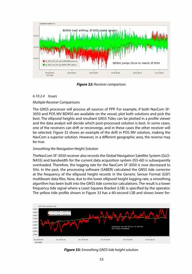
53

6.10.2.4 Issues

Multiple Receiver Comparisons

The GNSS processor will process all sources of PPP. For example, if both NavCom SF-3050 and POS MV BD950 are available on the vessel, plot both solutions and pick the best. The ellipsoid heights and resultant GNSS Tides can be plotted in a profile viewer and the data analyst will decide which post-processed solution is best. In some cases, one of the receivers can drift or reconverge, and in these cases the other receiver will be selected. Figure 32 shows an example of the drift in POS MV solution, making the NavCom a superior solution. However, in a different geographic area, the reverse may be true.

Smoothing the Navigation Height Solution

TheNavCom SF-3050 receiver also records the Global Navigation Satellite System (GLO-NASS) and bandwidth for the current data acquisition system (ISS-60) is subsequently overloaded. Therefore, the logging rate for the NavCom SF-3050 is now decreased to 5Hz. In the past, the processing software (SABER) calculated the GNSS tide corrector at the frequency of the ellipsoid height records in the Generic Sensor Format (GSF) multibeam data files. Now, due to the lower ellipsoid height logging rate, a smoothing algorithm has been built into the GNSS tide corrector calculations. The result is a lower frequency tide signal where a Least Squares Bracket (LSB) is specified by the operator. The yellow tide profile shown in Figure 33 has a 60-second LSB and shows lower fre-

Figure 32: Receiver comparison.

Figure 33: Smoothing GNSS tide height solution.

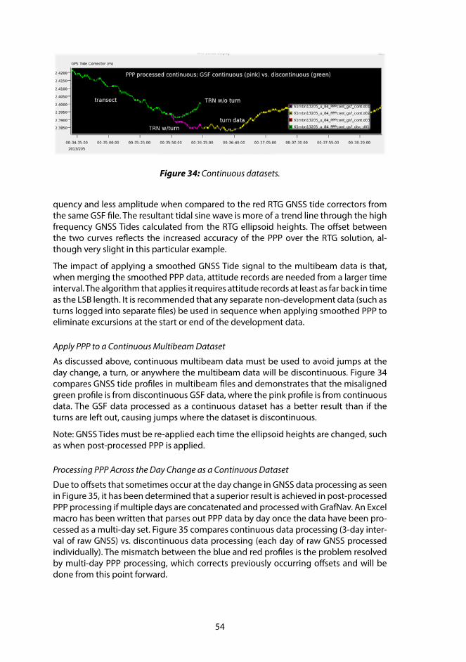
54

quency and less amplitude when compared to the red RTG GNSS tide correctors from the same GSF file. The resultant tidal sine wave is more of a trend line through the high frequency GNSS Tides calculated from the RTG ellipsoid heights. The offset between the two curves reflects the increased accuracy of the PPP over the RTG solution, al-though very slight in this particular example.

The impact of applying a smoothed GNSS Tide signal to the multibeam data is that, when merging the smoothed PPP data, attitude records are needed from a larger time interval. The algorithm that applies it requires attitude records at least as far back in time as the LSB length. It is recommended that any separate non-development data (such as turns logged into separate files) be used in sequence when applying smoothed PPP to eliminate excursions at the start or end of the development data.

Apply PPP to a Continuous Multibeam Dataset

As discussed above, continuous multibeam data must be used to avoid jumps at the day change, a turn, or anywhere the multibeam data will be discontinuous. Figure 34 compares GNSS tide profiles in multibeam files and demonstrates that the misaligned green profile is from discontinuous GSF data, where the pink profile is from continuous data. The GSF data processed as a continuous dataset has a better result than if the turns are left out, causing jumps where the dataset is discontinuous.

Note: GNSS Tides must be re-applied each time the ellipsoid heights are changed, such as when post-processed PPP is applied.

Processing PPP Across the Day Change as a Continuous Dataset

Due to offsets that sometimes occur at the day change in GNSS data processing as seen in Figure 35, it has been determined that a superior result is achieved in post-processed PPP processing if multiple days are concatenated and processed with GrafNav. An Excel macro has been written that parses out PPP data by day once the data have been pro-cessed as a multi-day set. Figure 35 compares continuous data processing (3-day inter-val of raw GNSS) vs. discontinuous data processing (each day of raw GNSS processed individually). The mismatch between the blue and red profiles is the problem resolved by multi-day PPP processing, which corrects previously occurring offsets and will be done from this point forward.

Figure 34: Continuous datasets.

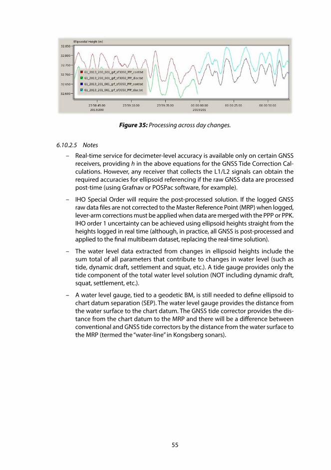
55

6.10.2.5 Notes

– Real-time service for decimeter-level accuracy is available only on certain GNSS receivers, providing h in the above equations for the GNSS Tide Correction Cal-culations. However, any receiver that collects the L1/L2 signals can obtain the required accuracies for ellipsoid referencing if the raw GNSS data are processed post-time (using Grafnav or POSPac software, for example).

– IHO Special Order will require the post-processed solution. If the logged GNSS raw data files are not corrected to the Master Reference Point (MRP) when logged, lever-arm corrections must be applied when data are merged with the PPP or PPK. IHO order 1 uncertainty can be achieved using ellipsoid heights straight from the heights logged in real time (although, in practice, all GNSS is post-processed and applied to the final multibeam dataset, replacing the real-time solution).

– The water level data extracted from changes in ellipsoid heights include the sum total of all parameters that contribute to changes in water level (such as tide, dynamic draft, settlement and squat, etc.). A tide gauge provides only the tide component of the total water level solution (NOT including dynamic draft, squat, settlement, etc.).

– A water level gauge, tied to a geodetic BM, is still needed to define ellipsoid to chart datum separation (SEP). The water level gauge provides the distance from the water surface to the chart datum. The GNSS tide corrector provides the dis-tance from the chart datum to the MRP and there will be a difference between conventional and GNSS tide correctors by the distance from the water surface to the MRP (termed the “water-line” in Kongsberg sonars).

Figure 35: Processing across day changes.

56

7 CONCLUSIONS AND RECOMMENDATIONS

GNSS has been used for horizontal positioning in hydrography for many years. Al-though vitally important in hydrography, understanding the technology and position computation process has not been necessary to use GNSS effectively. This is not the case for vertical positioning. In order to use the vertical component effectively, high-accuracy GNSS processing techniques must be used. It is essential that the user under-stand the uncertainties associated with the results, and be able to determine when and why a vertical position is unusable. The vertical uncertainty requirements in hydrogra-phy are far more stringent than in the horizontal, and the uncertainty associated with the vertical component of GNSS tends to be higher (2 to 3 times) than that achievable in the horizontal.

The use of the vertical component of GNSS should not completely replace tide gauges and heave sensors. Tide gauges should be installed and monitored as before to verify GPS observations and to validate separation models. Heave sensors should continue to be used to validate and augment the GNSS height observations.

Raw GNSS data should be collected on the vessel at all times, even if real-time pro-cesses are being used. If raw data are not recorded, any inconsistencies in the real-time solution will not be recoverable, resulting in lost data. GNSS data should be collected whenever possible, even if the vessel is in port. Constant monitoring of the water level will help with offset calibration and separation model validation. At the very least, high-accuracy GNSS observations should be available for the entire survey day, including transit to and from the survey site, and not only during survey lines.

Height offsets should be calibrated prior to and after the completion of a project.

It is essential that any depth products resulting from translation through a separation model be accompanied by appropriate metadata. This metadata must include the ver-tical datum of the dataset and how that datum was achieved. It must also include the vertical reference used for the GNSS computations, including epoch (e.g. IGS08 epoch 2012.9089).

Evaluation of GNSS observations used for vertical positioning in hydrography is ex-tremely important for bathymetric quality control. Any vertical fluctuations in the posi-tions due to GNSS processing will migrate directly into the representation of the bot-tom. Having the tools and information to help in this evaluation will greatly enhance the hydrographer’s confidence in the results. Information needed for this evaluation includes heave and tidal observations as well as uncertainty estimates from the GNSS processing software. Tools to help in this evaluation include graphical representation of heave, tide, GPS height, GPS vertical uncertainty GPS Tide. Filters to help identify changes in uncertainty or deviations from heave and/or tide observation would also be of assistance.

The most critical outstanding issues associated with ERS are the development of sepa-ration models and uncertainty estimates associated with those models.

It is relatively a simple task to develop a SEP surface for a small regional survey. The process becomes more complex when dealing with a national or multi-national pro-gram. Whatever method is used to develop multiple or single separation surfaces, it is essential that the references for all surfaces be clearly defined, and that a mechanism is in place to track any translations that are applied to hydrographic data.

57

The following is a summary of the recommendations for best practices in ERS.

1. Where practical, use RTK and/or PPK as the primary positioning method

2. Use PPP as a back-up and as primary if necessary

3. Until RTG reaches lower uncertainty, it should be used for real-time data acquisition, but replaced by PPP or RTK (if practical) in post-processing.

4. Always record and archive raw GNSS and motion observations

5. If using a base station, adhere to strict installation and data recording protocols, especially when recording antenna heights.

6. Perform a vertical positioning evaluation to ensure the system in use will meet the required uncertainty. This could be done in conjunction with the water-level gauge side-by-side validation (see below).

7. Continue to record real-time heave for data validation, even if it is not used in the final solution.

8. Perform side-by-side validation at an established water level gauge at the beginning and end of each project. Comparisons should take place over an entire tide cycle, or at a minimum three hours.

9. When using bottom mounted gauges, perform simultaneous GNSS observation sessions at the site during deployment and recover. These sessions should be at least 3 hours.

10. Use the NGS/IGS average values from the absolute calibration sheets for antenna phase center offset values.

11. It is necessary to monitor the GNSS solution to detect any precise positioning outages. Having a tool set that can display heave, GNSS height, height uncertainty and observed tide can facilitate the editing of suspect areas. Automatic filtering tools should also be used to detect times where the GNSS height uncertainty exceeded some criteria. Viewing a standard deviation surface early in the data processing/evaluation stream should also be used to identify potential problem areas.

12. The vertical uncertainty from the GNSS observation and computation process must be included in the final depth uncertainty determination. Translation of that position to the RP must also be taken into account. Care must be taken to insure inclusion only of those component uncertainties corresponding to parameters directly influencing the derived depths. Given this, component uncertainties from heave, static draft, loading draft, and dynamic draft may not contribute. Likewise, the component uncertainties associated with conventional water level correction (tide observations, tidal zoning) will not contribute to the ERS based TPU model.

13. The angular offsets of the motion sensor with respect to the reference frame need to be measured during the alignment survey. These offsets need to be programmed into the motion sensor and accounted for to ensure that the roll, pitch, and heading values truly reflect the orientation of the platform’s frame of reference. Misalignment of pitch or roll (WRT the platform) will directly increase the uncertainty of the derived depths when using an ERS workflow.

58

14. It is recommended that a water level gauge be used during a survey. This will provide a back-up in case of GNSS outages and provide QC for GNSS height validation. The gauge data can also be used to validate or even enhance the separation model.

15. It is recommended that any interpolation of SEP values between gauges include a geoid model. This is a reasonably simple method for developing a first estimate of an SEP model. Sea surface topography and hydrodynamic modeling should be incorporated into the model as that information becomes available.

16. It is recommended that those starting to use ERS continue to conduct surveys using traditional means and compare the ERS derived results. It is not necessary to go as far as developing seafloor surfaces from both methods. Simply comparing tides for each line determined using both methods (GNSS tides and traditional tides) will suffice.

17. Determining uncertainty in SEP modeling is a topic of discussion in the industry and all those using, or planning to use, ERS are encouraged to participate.

18. It is not important where in the processing stream that the translation from ellipsoid to chart datum takes place, as long as it is documented. Separation models must have associated metadata to indicate what they translate between, including epochs. Resulting surfaces should also contain this information. Regardless of where the translations take place, it is essential that it be possible to translate back to the original ellipsoid surface if necessary. If separation models are applied in real-time, all data related to that translation must be recorded (including the RTK observations).

19. When data are archived it is essential that they be accompanied with metadata that clearly defines exactly what translations have been applied. Separation models also need metadata attached that will identify epochs and reference datums. Ideally, data should be archived relative to the most stable surface (e.g. reference ellipsoid) and all separation and translation surfaces should be related to it. If this is the case, the original data and reference would not change, only the separation models to get it to another datum (geoid, chart ...) would change. However, this may take time because most historic data holdings are related to chart datum. The key is proper metadata management.

20. Unless the area is very small, always include a geoid model for interpolation between water level gauges

21. When applying Topography of the Sea Surface (TSS), water level gauge observation can be used near shore and MDT (derived from MSS) from satellite altimetry for the offshore

22. MSL to CD is the most problematic translation. Water level gauges provide the primary link at discrete locations along the shore, with interpolation and/or hydrodynamic modeling for intermediate locations, and hydrodynamic modeling for extrapolation into the offshore.

23. SEP surfaces should be validated through water level gauge observation on shore and water level gauge buoy (or bottom mounted gauge) observations in the offshore.

59

24. It is essential that a SEP naming convention be developed and metadata be attached to the surfaces as well as hydrographic survey deliverables that have been translated by a SEP surface.

Recommendations for future ERS discussions include:

1. ERS and SEP uncertainty

2. Detailed SEP development

3. Standardized SEP model data structures in the S-100 family, similar to the S-102 BAG.

4. Separation surface validation and densification

5. Inclusion of an ERS discussion in IHO C-13 Manual on Hydrography

6. Potential for a “Global” SEP

7. Connection of adjacent national SEP models.

REFERENCES

Adams, R., J. Iliffe, M. Ziebart, J. Turner and J. Oliveira, (2006). “Joining up Land and Sea.” GIM International, December 2006, volume 10, number 10.

Adams, R. (2006). “The Development of a Vertical Reference Surface and Model for Hydrography – a Guide.” Paper for the XXIII International FIG Conference. Munich, Germany, October 8–13, 2006. Taken from http://www.fig.net/pub/fig2006/papers/ts19/ts19_04_adams_0719.pdf

Arroyo-Suarez, E., D. Mabey, V. Hsiao, R. Phillips (2005). “Implementation of a Position-ing and Telemetry Buoy to Determine Chart Datum for Hydrographic Survey Applications.” Proceedings of the 2005 ION GNSS Conference, September 13–16, 2005. Long Beach, CA.

Bilich, A., G. Mader (2010). “GNSS Absolute Antenna Calibration at the National Geo-detic Survey.” Proceedings of the 2010 ION GNSS Conference, September 21–24, 2010. Portland, OR.

de Lange Boom, B. (2012). “Vertical Separation Models for the British Columbian Coast.” Canadian Hydrographic Conference 2012 proceedings, Niagara Falls, Canada, 2012.

de Lange Boom, B., M. Craymer, A. Godin, T. Heron, D. Lefaivre, P. MacAulay, C. Robin, J. Haung, P. Héroux, C. Clatt and M. Véronneau (2012). “CHS National Project: Continuous Vertical Datums for Canadian Waters.” Unpublished Progress and Planning Report by DFO-CHS and NRCan-GSD, December 2012.

de Lange Boom, B., J. Bartlett, M. Craymer, A. Godin, T. Heron, D. Lefaivre, P. MacAulay, L. Maltais, S. Nudds, C. Robin, and M. Véronneau (2013). “CHS National Project: Continuous Vertical Datums for Canadian Waters.” Unpublished status summary by DFO-CHS and NRCan-GSD, February 2013.

60

Dodd. D., B. Mehaffey, G. Smith, K. Barbor, S. O’Brien, M. van Norden (2009). “Chart Datum Transfer Using a GPS Tide Gauge Buoy in Chesapeake Bay.” International Hydrographic Review, November 2009 on-line edition. (http://www.iho-ohi.net/mtg_docs/IHReview/2009/IHR_Intro.htm)

Dodd D., J. Mills, D. Battilana, M. Gourley (2010). “Hydrographic Surveying Using the Ellipsoid as the Vertical Reference Surface.” Proceedings of the FIG Congress 2010, April 11–16, Sydney, Australia

Dodd D. and J. Mills, (2011). “Ellipsoidally Referenced Surveys (ERS); Issues and Solu-tions.” International Hydrographic Review, November 2011 on-line edition.

Dodd D. and J. Mills, (2012). “Ellipsoidally Referenced Surveys (ERS); Separation Mod-els.” Proceedings of the FIG Working Week 2012. May 06 to 10, 2012. Rome, Italy.

Elenbaas, B. (2012). “Creating a Local SEP Surface.” Unpublished presentation image.

FIG, (2006). “FIG Guide on the Development of a Vertical Reference Surface for Hydrography.” FIG Publication No 37 produced by Commissions 4 and 5, Working Group 4.2.

Forsberg, R., G. Strykowski, O. Andersen (2011). “Final VRF Grids.” BLAST project refer-ence document. Taken from http://blast-project.eu/?page=articles&artid=167, accessed February 24, 2012.

Gill, S.K. and J.R. Schultz (2001). “Tidal Datums and Their Applications”, NOAA Special Publication NOS CO-OPS 1.

Gesch, D. and R. Wilson (2001). “Development of a Seamless Multisource Topographic / Bathymetric Elevation Model for Tampa Bay.” Marine Technology Society Jour-nal, 35(4):58–64, Winter 2001/2002. Taken from http://dl.cr.usgs.gov/net_prod_download/public/gom_net_pub_products/doc/mtsjournal.pdf

Guenther, G., A. G. Cunningham, P. E. LaRocque, and D. J. Reid (2000). Meeting the Accuracy Challenge in Airborne Lidar Bathymetry. Proceedings of EARSeL-SIG-Workshop LIDAR, Dresden/FRG, June 16 – 17, 2000

Guenther, G. (2001). “Digital Elevation Model Technologies and Applications, The DEM Users Manual: Chapter 8 Airborne Lidar Bathymetry.” American Society for Photogrammetry and Remote Sensing. Bethesda, MA, USA.

Hess, K.W. (2002). “Spatial interpolation of tidal data in irregularly-shaped coastal re-gions by numerical solution of Laplace’s equation”, Estuarine, Coastal and Shelf Science, 54, 175 – 192.

Howlett, C. (2009). “VORF: A Model for Surveying to the Ellipsoid.” Presentation to the Hydrographic Society, November 26, 2009. Aberdeen. Taken from http://www.ths.org.uk/, access February 23, 2012.

IHO (International Hydrographic Organization), ”Manual on Hydrography”, 1st Edition, May 2005 on-line edition: (http://www.iho-ohi.net/iho_pubs/CB/C13_Index.htm)

Lefaivre, D., A. Godin, D. Dodd, T. Herron, P. MacAulay, D. Sinnott (2010). “The Continuous Vertical Datum Canadian Waters Project (Beginnings, Vision, Methods and Progress).” Poster for the Canadian Hydrographic Conference, June 2010, Quebec City.

61

Lévesque, S., B. de Lange Boom, J. Bartlett, M. Craymer, A. Godin, T. Heron, D. Lefaivre, P. MacAulay, L. Maltais, S. Nudds, C. Robin, M. Véronneau (2013). “Canadian Hydrographic Service Activities for 2012–2013 Relating to the Canadian Spatial Reference System.” Unpublished report for the Canadian Geodetic Reference System Committee’s annual meeting, April 22–24, 2013.

Luettich, R.A., J.J Westerink and N.W. Scheffner (1992). ADCIRC: An Advanced Three-Dimensional Circulation Model for Shelves, Coasts, and Estuaries, Technical Report DRP-92-6, U.S. ACE Waterways Experiment Station, Vicksburg, MS.

Milbert, D. G. (2002). “Documentation for VDatum and a datum tutorial: Vertical datum transformation software, version 1.06.”

Mukai, A., J.J. Westerink, R.A. Luettich and D. Mark (2001). “A Tidal Constituent Data-base for the Western North Atlantic Ocean, Gulf of Mexico and Caribbean Sea. Technical Report”, U.S. Army Engineer Research and Development Center, Vicks-burg, MS.

NASA, 2009. “Ocean Dynamic Topography.” Image from NASA JPL Science Data Gallery website. http://sealevel.jpl.nasa.gov/gallery/science.html. Accessed June, 2009.

NOAA, (2007). “Topographic and Bathymetric Data Considerations: Datums, Datum Conversion Techniques, and Data Integration Part II of A Roadmap to a Seam-less Topobathy Surface.” NOAA Technical Report NOAA/CSC/20718-PUB.

NOAA, (2011). “Estimation of Vertical Uncertainties in VDatum.” NOAA Vertical Datum Transformation document. Taken from http://vdatum.noaa.gov/download/publications/Estimation_of_Vertical_Uncertainties_in_VDatum_7_2011.pdf, accessed February 24, 2012

Oliveira A.M., E. Arroyo-Suarez, A. Ramos, M. Arentz, (2010). “Seabed Mapping on an Earth Centered Earth Fixed (ECEF) Geocentric Reference Frame. Cooperative Validation with US Navy and Brazilian Navy in Guanabara Bay, Rio de Janeiro”. Proceedings of ION GNSS 2010, September 21–24, 2010, Portland OR.

Olsson, U., (2009). Email communication, August 31, 2009.

Rice, (2011). “Measuring the Water Level Datum Relative to the Ellipsoid During Hydrographic Survey.” Paper accepted for publication in the proceedings of U.S. Hydro 2011. April 25–28, 2011. Tampa, FL.

Robin, C. and S. Nudds (2013). CVDCW 2013 Workshop Power Point.

Robin, C., A. Godin, P. MacAulay, B. de Lange Boom, D. Lefaivre, T. Herron, D. Sinnott, A. Ballantyne, L. Maltais, and M. Véronneau (2012). “The Canadian Hydrographic Continuous Vertical Datum: Methodology and Accuracy.” Canadian Hydro-graphic Conference 2012 proceedings, Niagara Falls, Canada, 2012.

Robin, CI., (2013). “SEP Protocol, Part I: Adjust Model Datums.” Unpublished document for Continuous Vertical Datum Canadian Waters procedures.

Robin, CII., (2013). “SEP Protocol, Part II: Attach adjusted model datums to MWL.” Unpub-lished document for Continuous Vertical Datum Canadian Waters procedures.

Robin, CIII., (2013). “SEP Protocol, Part III: Difference Layer(s).” Unpublished document for Continuous Vertical Datum Canadian Waters procedures.

62

Strykowski G., O. B. Andersen, I. Einarsson, R. Forsberg, L. Doorst, T. Ligteringen (2011). “BLAST Vertical Datums: Overview, Conventions and Recommendations.” BLAST project reference document.

Taken from http://blast-project.eu/?page=articles&artid=167, accessed February 24, 2012.

Todd, P., RJ. Martin, GJ. Broadbent (2004). “Infrastructure Supporting Mapping of Tidal Planes and Lines.” Paper for the 4th Trans Tasman Surveyors Conference 2004. Auckland, NZ.

Vignudelli, S., P. Berry, L. Roblou,(2008). “Satellite Altimetry Near Coasts – Current Practices and a Look at the Future.” Submitted to the book “15 Years of Pro-gress in Radar Altimetry” (16 April 2008). Taken from http://www.alticore.eu/ Publications/paper_vignudelli_et_al_ESA_2008.pdf, accessed February 20, 2012.

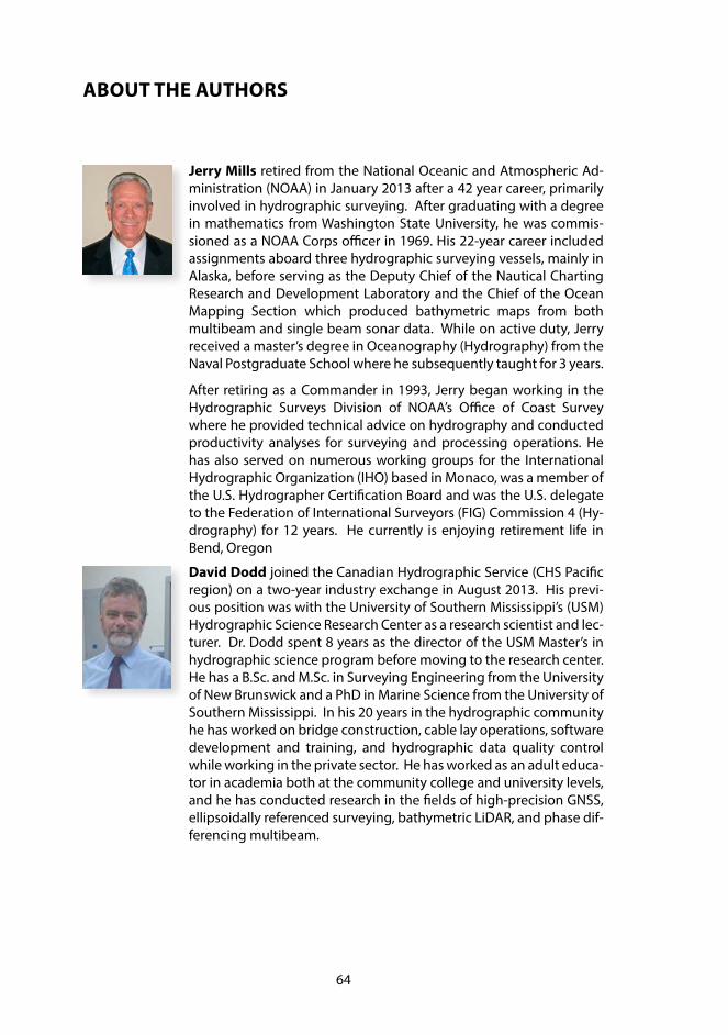
64

ABOUT THE AUTHORS

Jerry Mills retired from the National Oceanic and Atmospheric Ad-ministration (NOAA) in January 2013 after a 42 year career, primarily involved in hydrographic surveying. After graduating with a degree in mathematics from Washington State University, he was commis-sioned as a NOAA Corps officer in 1969. His 22-year career included assignments aboard three hydrographic surveying vessels, mainly in Alaska, before serving as the Deputy Chief of the Nautical Charting Research and Development Laboratory and the Chief of the Ocean Mapping Section which produced bathymetric maps from both multibeam and single beam sonar data. While on active duty, Jerry received a master’s degree in Oceanography (Hydrography) from the Naval Postgraduate School where he subsequently taught for 3 years.

After retiring as a Commander in 1993, Jerry began working in the Hydrographic Surveys Division of NOAA’s Office of Coast Survey where he provided technical advice on hydrography and conducted productivity analyses for surveying and processing operations. He has also served on numerous working groups for the International Hydrographic Organization (IHO) based in Monaco, was a member of the U.S. Hydrographer Certification Board and was the U.S. delegate to the Federation of International Surveyors (FIG) Commission 4 (Hy-drography) for 12 years. He currently is enjoying retirement life in Bend, Oregon

David Dodd joined the Canadian Hydrographic Service (CHS Pacific region) on a two-year industry exchange in August 2013. His previ-ous position was with the University of Southern Mississippi’s (USM) Hydrographic Science Research Center as a research scientist and lec-turer. Dr. Dodd spent 8 years as the director of the USM Master’s in hydrographic science program before moving to the research center. He has a B.Sc. and M.Sc. in Surveying Engineering from the University of New Brunswick and a PhD in Marine Science from the University of Southern Mississippi. In his 20 years in the hydrographic community he has worked on bridge construction, cable lay operations, software development and training, and hydrographic data quality control while working in the private sector. He has worked as an adult educa-tor in academia both at the community college and university levels, and he has conducted research in the fields of high-precision GNSS, ellipsoidally referenced surveying, bathymetric LiDAR, and phase dif-ferencing multibeam.

65

FIG PUBLICATIONS

The FIG publications are divided into four categories. This should assist members and other users to identify the profile and purpose of the various publications.

FIG Policy StatementsFIG Policy Statements include political declarations and recommendations endorsed by the FIG General Assembly. They are prepared to explain FIG policies on important topics to politicians, government agencies and other decision makers, as well as sur-veyors and other professionals.

FIG GuidesFIG Guides are technical or managerial guidelines endorsed by the Council and record-ed by the General Assembly. They are prepared to deal with topical professional issues and provide guidance for the surveying profession and relevant partners.

FIG ReportsFIG Reports are technical reports representing the outcomes from scientific meetings and Commission working groups. The reports are approved by the Council and include valuable information on specific topics of relevance to the profession, members and individual surveyors.

FIG RegulationsFIG Regulations include statutes, internal rules and work plans adopted by the FIG or-ganisation.

List of FIG publicationsFor an up-to-date list of publications, please visit www.fig.net/pub/figpub

ABOUT FIG

International Federation of Surveyors is the premier international or-ganization representing the interests of surveyors worldwide. It is a fed-eration of the national member associations and covers the whole range of professional fields within the global surveying community. It provides an international forum for discussion and development aiming to pro-mote professional practice and standards.

FIG was founded in 1878 in Paris and was first known as the Fédération Internationale des Géomètres (FIG). This has become anglicized to the International Federation of Sur-veyors (FIG). It is a United Nations and World Bank Group recognized non-government organization (NGO), representing a membership from 120 plus countries throughout the world, and its aim is to ensure that the disciplines of surveying and all who practise them meet the needs of the markets and communities that they serve.

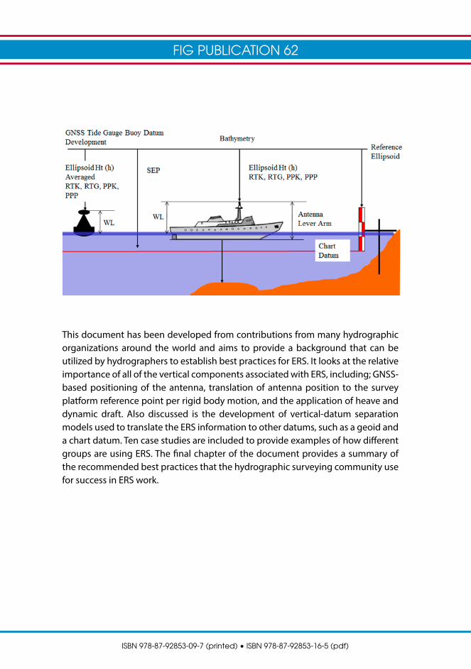
FIG PUBLICATION 62

ISBN 978-87-92853-09-7 (printed) • ISBN 978-87-92853-16-5 (pdf)

This document has been developed from contributions from many hydrographic organizations around the world and aims to provide a background that can be utilized by hydrographers to establish best practices for ERS. It looks at the relative importance of all of the vertical components associated with ERS, including; GNSS-based positioning of the antenna, translation of antenna position to the survey platform reference point per rigid body motion, and the application of heave and dynamic draft. Also discussed is the development of vertical-datum separation models used to translate the ERS information to other datums, such as a geoid and a chart datum. Ten case studies are included to provide examples of how different groups are using ERS. The final chapter of the document provides a summary of the recommended best practices that the hydrographic surveying community use for success in ERS work.

Documents

Ellipsoidally Referenced Surveying for Hydrography - FIG · Ellipsoidally Referenced Surveying for Hydrography ... Effect of vessel pitch on height translation to the vessel reference