L. Vandenberghe EE236C (Spring 2013-14)

Ellipsoid method

• ellipsoid method

• convergence proof

• inequality constraints

1

Ellipsoid method

history

• developed by Shor, Nemirovski, Yudin in 1970s

• used in 1979 by Khachian to show polynomial solvability of LPs

properties

• each step requires cutting-plane or subgradient evaluation

• modest storage (O(n2))

• modest computation per step (O(n2)), via analytical formula

• extremely simple to implement

• efficient in theory

• slow but steady in practice; rarely used

Ellipsoid method 2

Motivation

drawbacks of cutting-plane methods

• serious computation needed to find next query point

typically, O(n2m) for analytic centering in ACCPM, with m inequalities

• localization polyhedron grows in complexity as algorithm progresses

(with pruning, can keep m proportional to n, e.g., m = 4n)

ellipsoid method addresses both issues, but retains theoretical efficiency

Ellipsoid method 3

Ellipsoid algorithm for minimizing convex function

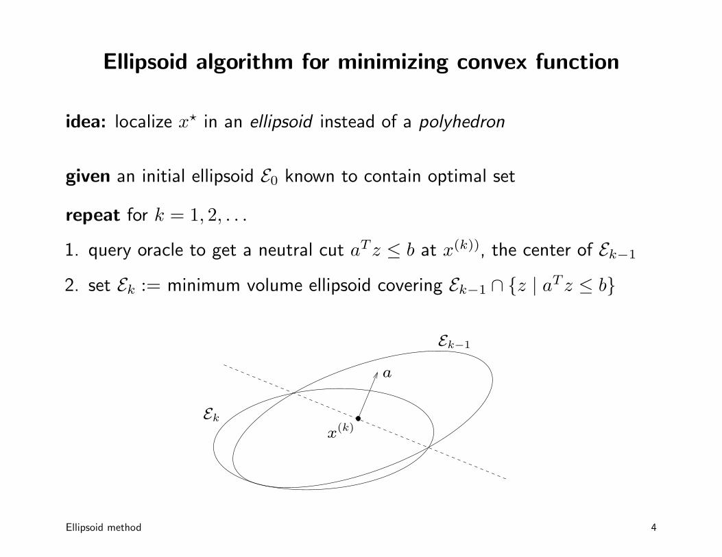
idea: localize x⋆ in an ellipsoid instead of a polyhedron

given an initial ellipsoid E0 known to contain optimal set

repeat for k = 1, 2, . . .

1. query oracle to get a neutral cut aTz ≤ b at x(k)), the center of Ek−1

2. set Ek := minimum volume ellipsoid covering Ek−1 ∩ {z | aTz ≤ b}

Ek−1

x(k)

a

Ek

Ellipsoid method 4

differences with cutting-plane methods

• localization set doesn’t grow more complicated

• generating query point is trivial

• but, we add unnecessary points in step 2

interpretation

• reduces to bisection for n = 1

• can be viewed as an implementable version of the center-of-gravitycutting-plane method

Ellipsoid method 5

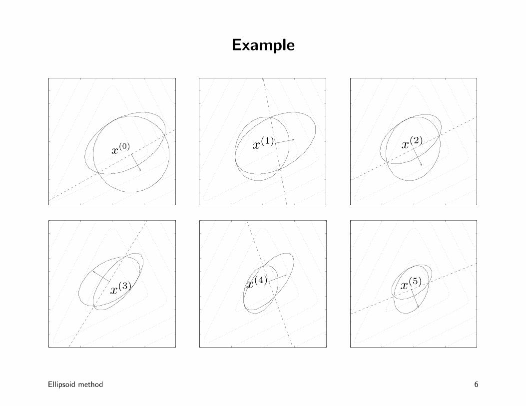
Example

♣x(0)♣x(1)

♣x(2)

♣

x(3)♣x(4)

♣x(5)

Ellipsoid method 6

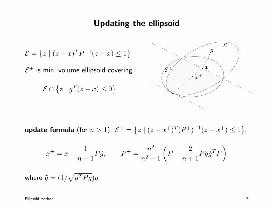
Updating the ellipsoid

E ={

z | (z − x)TP−1(z − x) ≤ 1}

E+ is min. volume ellipsoid covering

E ∩{

z | gT (z − x) ≤ 0}

rx

rx+

r

E

E+

g

update formula (for n > 1): E+ ={

z | (z − x+)T (P+)−1(z − x+) ≤ 1}

,

x+ = x−1

n+ 1P g̃, P+ =

n2

n2 − 1

(

P −2

n+ 1P g̃g̃TP

)

where g̃ = (1/√

gTPg)g

Ellipsoid method 7

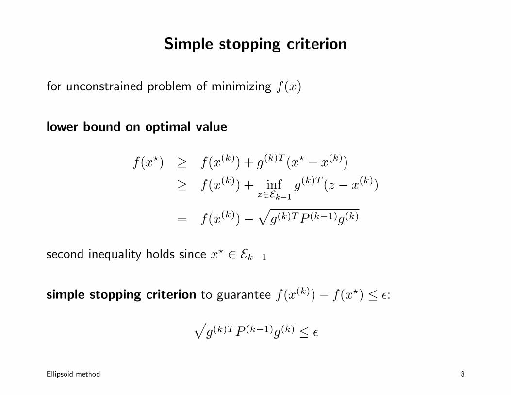
Simple stopping criterion

for unconstrained problem of minimizing f(x)

lower bound on optimal value

f(x⋆) ≥ f(x(k)) + g(k)T (x⋆ − x(k))

≥ f(x(k)) + infz∈Ek−1

g(k)T (z − x(k))

= f(x(k))−√

g(k)TP (k−1)g(k)

second inequality holds since x⋆ ∈ Ek−1

simple stopping criterion to guarantee f(x(k))− f(x⋆) ≤ ǫ:

√

g(k)TP (k−1)g(k) ≤ ǫ

Ellipsoid method 8

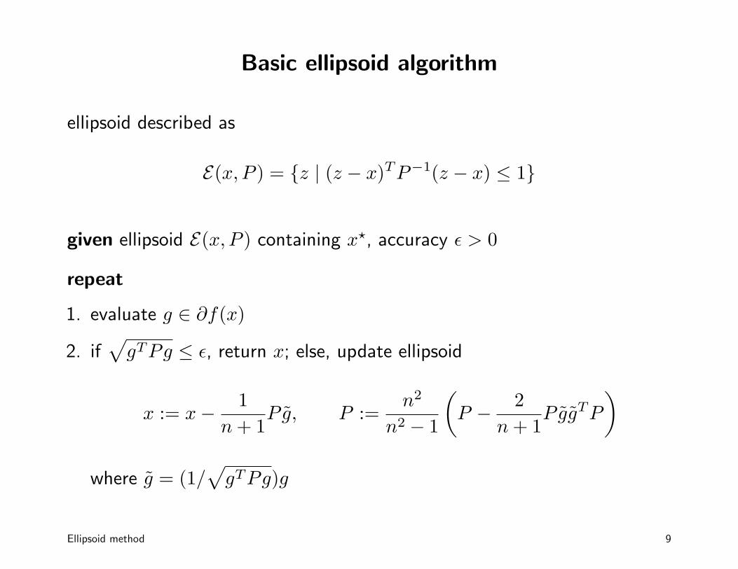
Basic ellipsoid algorithm

ellipsoid described as

E(x, P ) = {z | (z − x)TP−1(z − x) ≤ 1}

given ellipsoid E(x, P ) containing x⋆, accuracy ǫ > 0

repeat

1. evaluate g ∈ ∂f(x)

2. if√

gTPg ≤ ǫ, return x; else, update ellipsoid

x := x−1

n+ 1P g̃, P :=

n2

n2 − 1

(

P −2

n+ 1P g̃g̃TP

)

where g̃ = (1/√

gTPg)g

Ellipsoid method 9

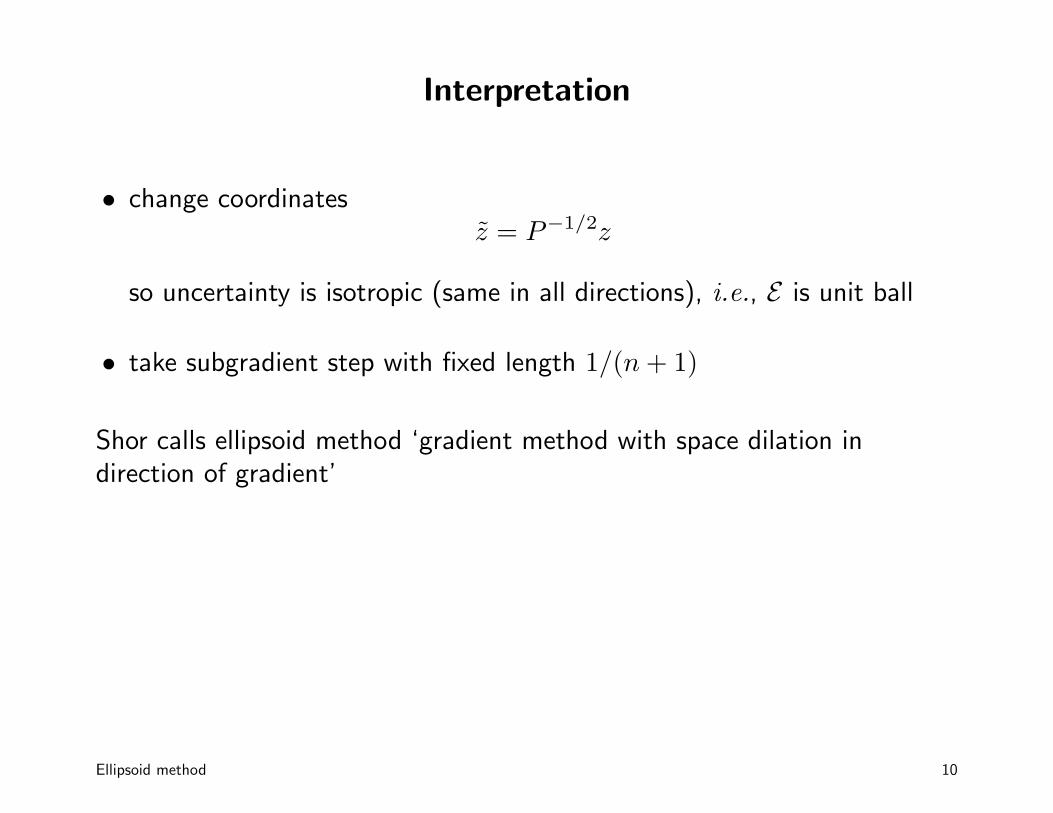
Interpretation

• change coordinatesz̃ = P−1/2z

so uncertainty is isotropic (same in all directions), i.e., E is unit ball

• take subgradient step with fixed length 1/(n+ 1)

Shor calls ellipsoid method ‘gradient method with space dilation indirection of gradient’

Ellipsoid method 10

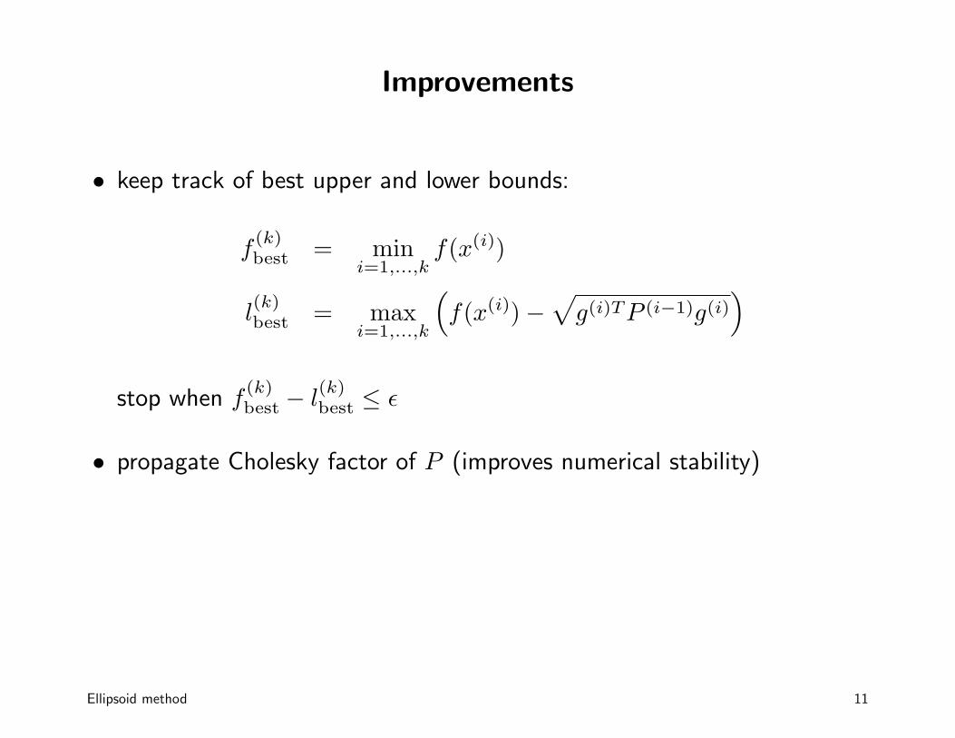
Improvements

• keep track of best upper and lower bounds:

f(k)best = min

i=1,...,kf(x(i))

l(k)best = max

i=1,...,k

(

f(x(i))−√

g(i)TP (i−1)g(i))

stop when f(k)best − l

(k)best ≤ ǫ

• propagate Cholesky factor of P (improves numerical stability)

Ellipsoid method 11

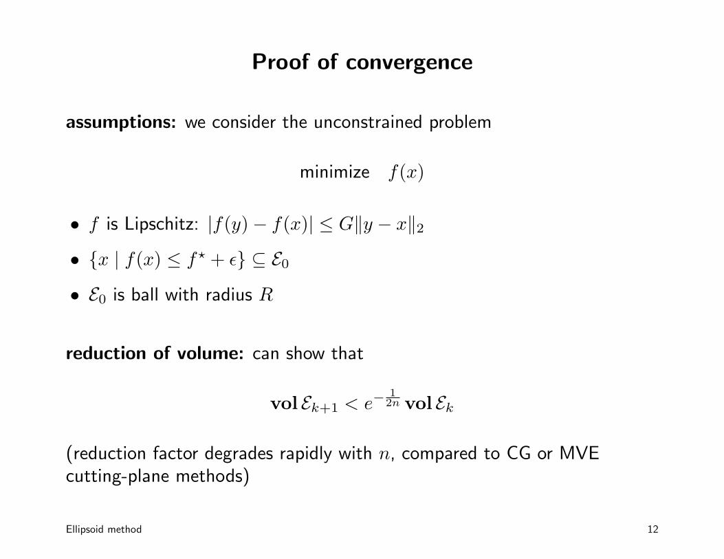
Proof of convergence

assumptions: we consider the unconstrained problem

minimize f(x)

• f is Lipschitz: |f(y)− f(x)| ≤ G‖y − x‖2

• {x | f(x) ≤ f⋆ + ǫ} ⊆ E0

• E0 is ball with radius R

reduction of volume: can show that

vol Ek+1 < e−12n vol Ek

(reduction factor degrades rapidly with n, compared to CG or MVEcutting-plane methods)

Ellipsoid method 12

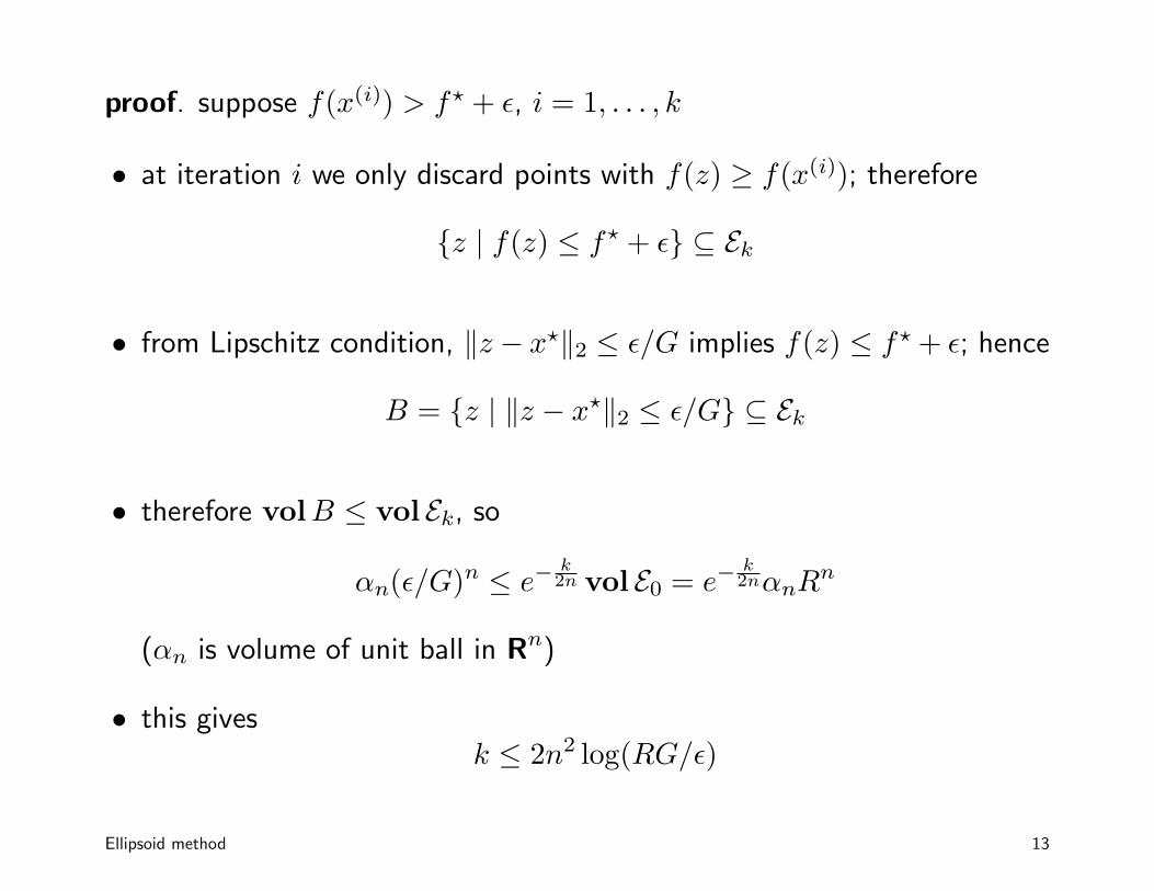
proof. suppose f(x(i)) > f⋆ + ǫ, i = 1, . . . , k

• at iteration i we only discard points with f(z) ≥ f(x(i)); therefore

{z | f(z) ≤ f⋆ + ǫ} ⊆ Ek

• from Lipschitz condition, ‖z − x⋆‖2 ≤ ǫ/G implies f(z) ≤ f⋆ + ǫ; hence

B = {z | ‖z − x⋆‖2 ≤ ǫ/G} ⊆ Ek

• therefore volB ≤ vol Ek, so

αn(ǫ/G)n ≤ e−k2n vol E0 = e−

k2nαnR

n

(αn is volume of unit ball in Rn)

• this givesk ≤ 2n2 log(RG/ǫ)

Ellipsoid method 13

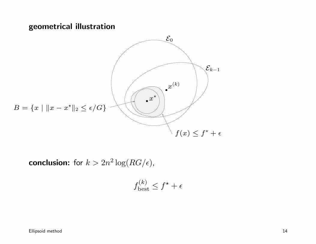
geometrical illustration

E0

Ek−1

x(k)

f(x) ≤ f⋆ + ǫ

B = {x | ‖x − x⋆‖2 ≤ ǫ/G}

x⋆

conclusion: for k > 2n2 log(RG/ǫ),

f(k)best ≤ f⋆ + ǫ

Ellipsoid method 14

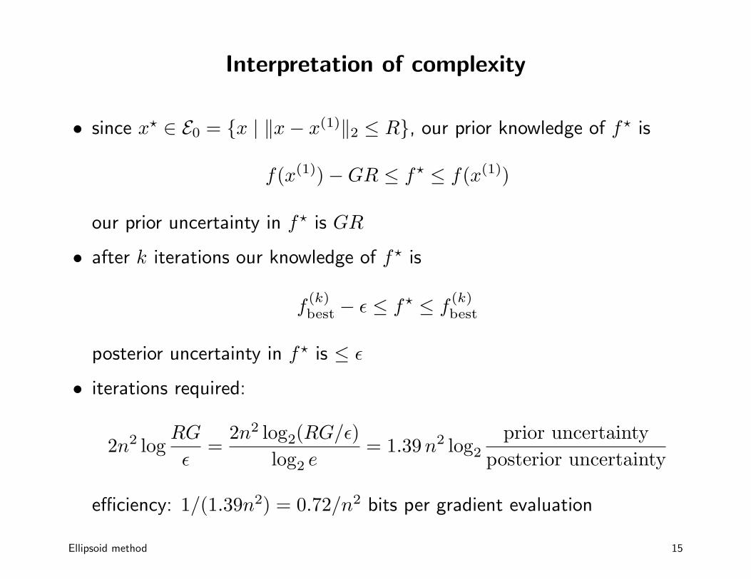
Interpretation of complexity

• since x⋆ ∈ E0 = {x | ‖x− x(1)‖2 ≤ R}, our prior knowledge of f⋆ is

f(x(1))−GR ≤ f⋆ ≤ f(x(1))

our prior uncertainty in f⋆ is GR

• after k iterations our knowledge of f⋆ is

f(k)best − ǫ ≤ f⋆ ≤ f

(k)best

posterior uncertainty in f⋆ is ≤ ǫ

• iterations required:

2n2 logRG

ǫ=

2n2 log2(RG/ǫ)

log2 e= 1.39n2 log2

prior uncertainty

posterior uncertainty

efficiency: 1/(1.39n2) = 0.72/n2 bits per gradient evaluation

Ellipsoid method 15

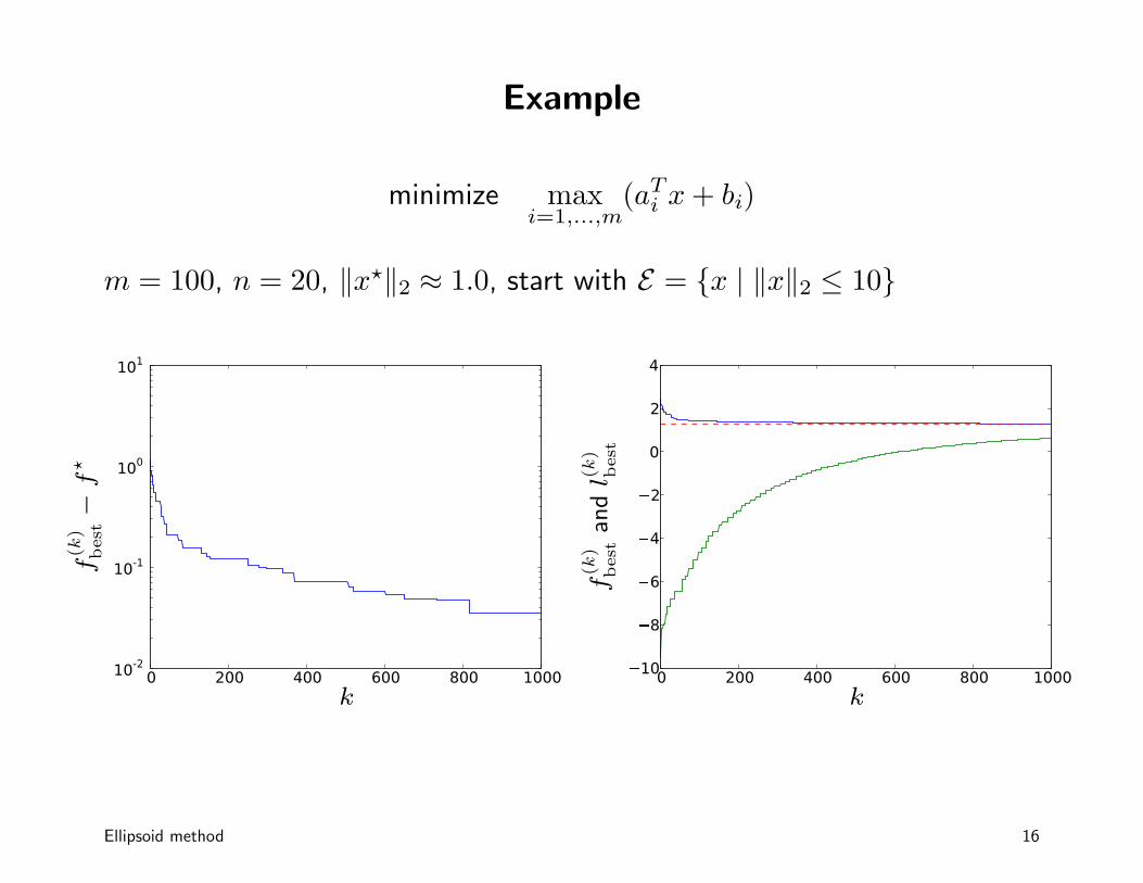
Example

minimize maxi=1,...,m

(aTi x+ bi)

m = 100, n = 20, ‖x⋆‖2 ≈ 1.0, start with E = {x | ‖x‖2 ≤ 10}

0 200 400 600 800 100010-2

10-1

100

101

k

f(k

)best−

f⋆

0 200 400 600 800 1000

� 10

� 8

� 6

� 4

� 2

0

2

4

k

f(k

)bestandl(k)

best

Ellipsoid method 16

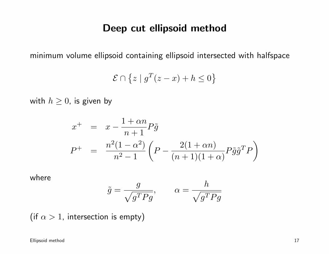
Deep cut ellipsoid method

minimum volume ellipsoid containing ellipsoid intersected with halfspace

E ∩{

z | gT (z − x) + h ≤ 0}

with h ≥ 0, is given by

x+ = x−1 + αn

n+ 1P g̃

P+ =n2(1− α2)

n2 − 1

(

P −2(1 + αn)

(n+ 1)(1 + α)P g̃g̃TP

)

where

g̃ =g

√

gTPg, α =

h√

gTPg

(if α > 1, intersection is empty)

Ellipsoid method 17

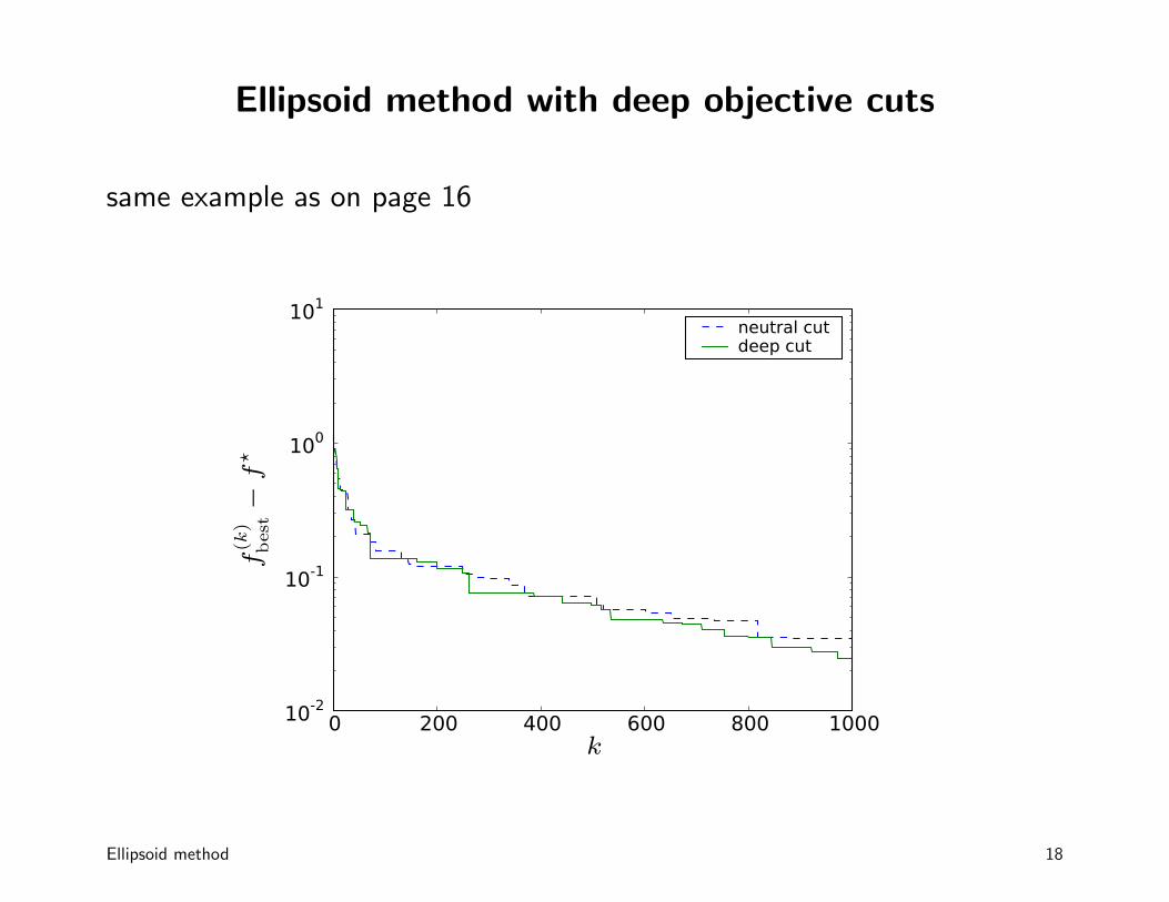
Ellipsoid method with deep objective cuts

same example as on page 16

0 200 400 600 800 100010-2

10-1

100

101

neutral cutdeep cut

k

f(k

)best−

f⋆

Ellipsoid method 18

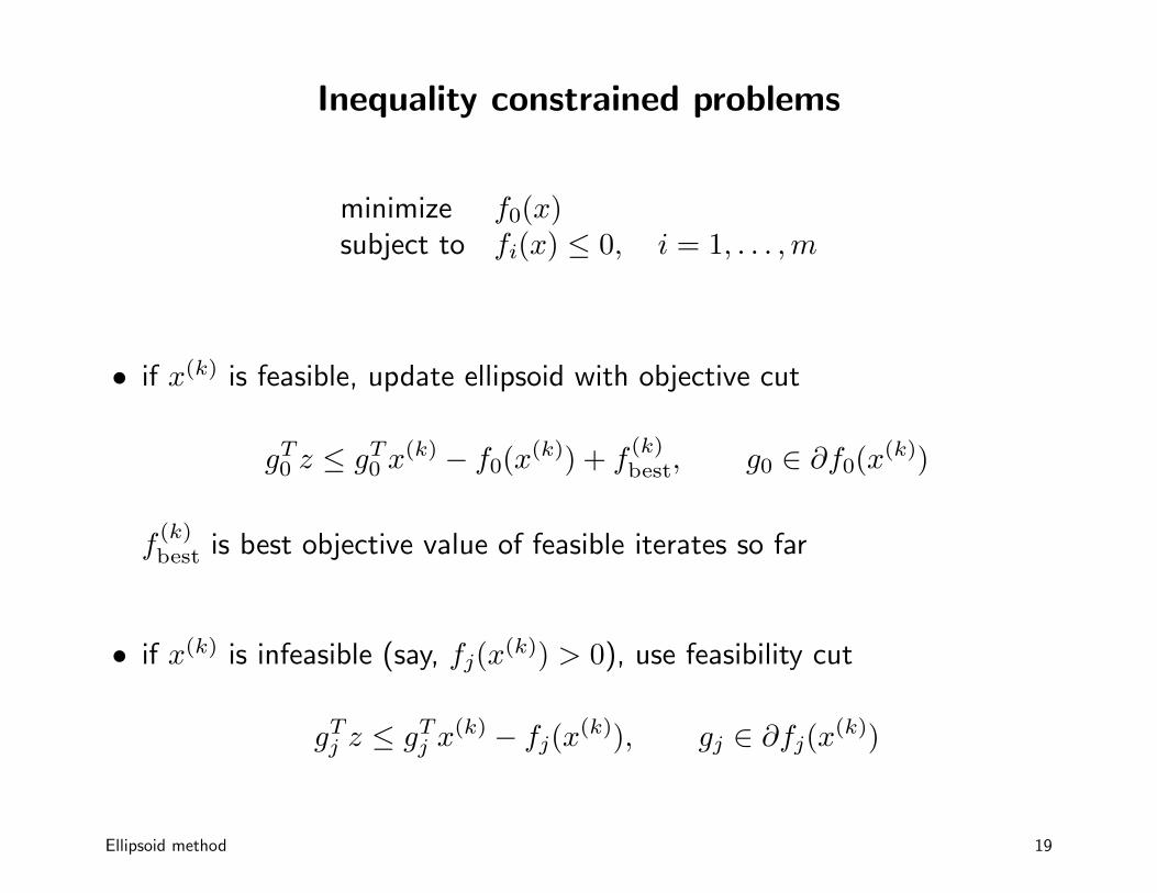
Inequality constrained problems

minimize f0(x)subject to fi(x) ≤ 0, i = 1, . . . ,m

• if x(k) is feasible, update ellipsoid with objective cut

gT0 z ≤ gT0 x(k) − f0(x

(k)) + f(k)best, g0 ∈ ∂f0(x

(k))

f(k)best is best objective value of feasible iterates so far

• if x(k) is infeasible (say, fj(x(k)) > 0), use feasibility cut

gTj z ≤ gTj x(k) − fj(x

(k)), gj ∈ ∂fj(x(k))

Ellipsoid method 19

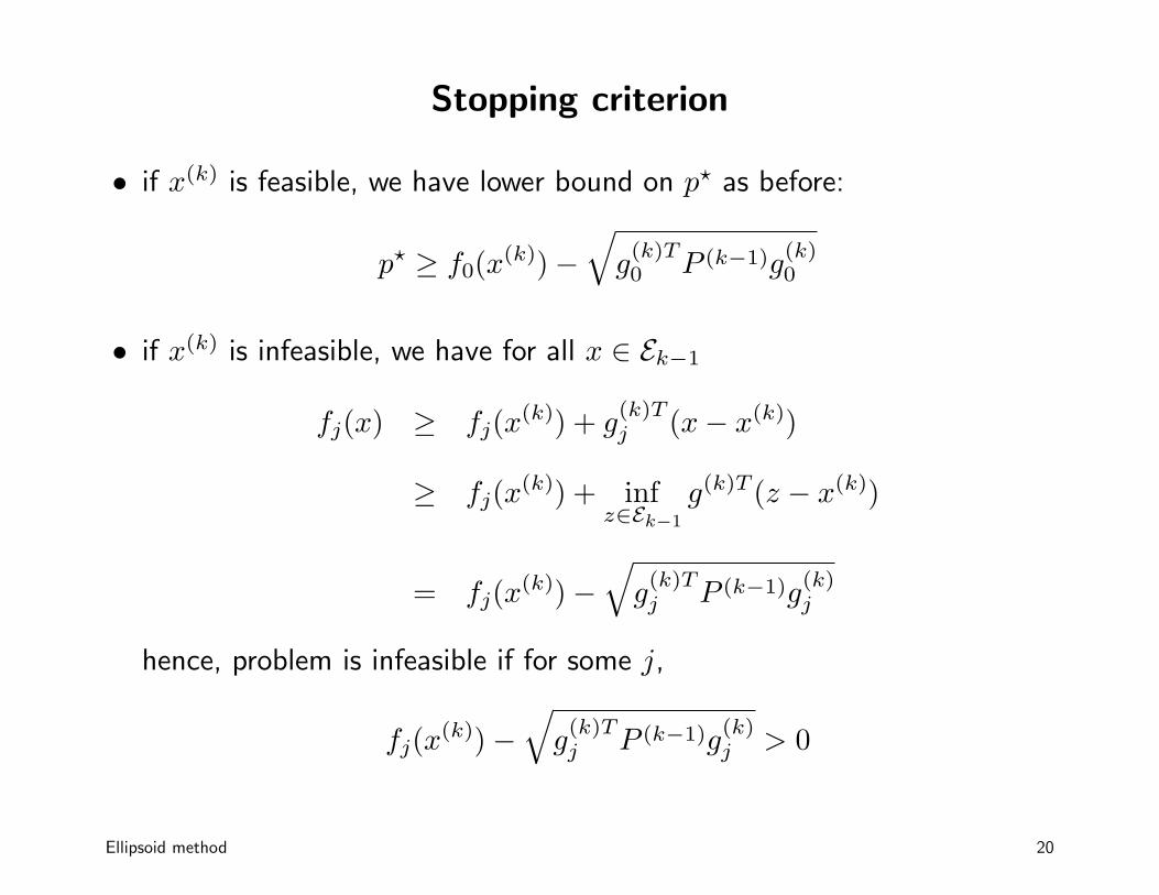
Stopping criterion

• if x(k) is feasible, we have lower bound on p⋆ as before:

p⋆ ≥ f0(x(k))−

√

g(k)T0 P (k−1)g

(k)0

• if x(k) is infeasible, we have for all x ∈ Ek−1

fj(x) ≥ fj(x(k)) + g

(k)Tj (x− x(k))

≥ fj(x(k)) + inf

z∈Ek−1

g(k)T (z − x(k))

= fj(x(k))−

√

g(k)Tj P (k−1)g

(k)j

hence, problem is infeasible if for some j,

fj(x(k))−

√

g(k)Tj P (k−1)g

(k)j > 0

Ellipsoid method 20

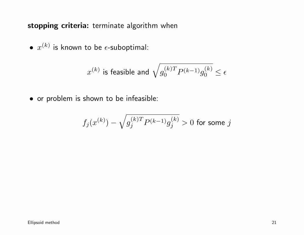
stopping criteria: terminate algorithm when

• x(k) is known to be ǫ-suboptimal:

x(k) is feasible and

√

g(k)T0 P (k−1)g

(k)0 ≤ ǫ

• or problem is shown to be infeasible:

fj(x(k))−

√

g(k)Tj P (k−1)g

(k)j > 0 for some j

Ellipsoid method 21