Pattern Recognition 46 (2013) 1449–1465

Contents lists available at SciVerse ScienceDirect

Pattern Recognition

0031-32

http://d

n Corr

E-m

asmkleu

journal homepage: www.elsevier.com/locate/pr

ElliFit: An unconstrained, non-iterative, least squares based geometricEllipse Fitting method

Dilip K. Prasad a,n, Maylor K.H. Leung b, Chai Quek a

a School of Computer Engineering, Nanyang Technological University, Singapore 639798, Singaporeb Faculty of Inform. & Comm. Tech., Universiti Tunku Abdul Rahman, Kampar, Malaysia

a r t i c l e i n f o

Article history:

Received 14 December 2011

Received in revised form

24 July 2012

Accepted 7 November 2012Available online 16 November 2012

Keywords:

Ellipse fitting

Shape analysis

Unconstrained optimization

Least squares method

03/$ - see front matter & 2012 Elsevier Ltd. A

x.doi.org/10.1016/j.patcog.2012.11.007

esponding author. Tel.: þ65 84220406.

ail addresses: dilipprasad@gmail.com (D.K. Pr

ng@gmail.com (M.K.H. Leung), ashcquek@nt

a b s t r a c t

A novel ellipse fitting method which is selective for digital and noisy elliptic curves is proposed in this

paper. The method aims at fitting an ellipse only when the data points are highly likely belong to an

ellipse. This is achieved using the geometric distances of the ellipse from the data points. The proposed

method models the non-linear problem of ellipse fitting as a combination of two operators, with one

being linear, numerically stable, and easily invertible, while the other being non-linear but unique and

easily invertible operator. As a consequence, the proposed ellipse fitting method has several salient

properties like unconstrained, stable, non-iterative, and computationally inexpensive. The efficacy of

the method is compared against six contemporary and recent algorithms based on the least squares

formulation using five experiments of diverse practical challenges, like digitization, incomplete ellipses,

and Gaussian noise (up to 30%). Three of the experiments comprise of a total of 44,400 ellipses (positive

test data) while the other two are tested on 320,000 non-elliptic conics (negative test data). The results

show that the proposed method is quite selective to elliptic shapes only and provides accurate fitting

results, indicating potential application in medical, robotics, object detection, and other image

processing industrial applications.

& 2012 Elsevier Ltd. All rights reserved.

1. Introduction

In many image processing applications, shape based analysisplays an important role and it is desirable to detect specificgeometrical shapes like polygons, ellipses, etc. Since ellipses arethe most common non-linear shapes in natural and man-madeobjects, detecting ellipses from images is very useful. For example,detecting ellipses from images is desired in application like pupiltracking, biological cell segmentation, astronomical and geologicalshape segmentation, object detection, etc.

While there are some sophisticated algorithms for detectingellipses from images, most of these algorithms cannot be used inreal time applications. Further, there is generally a least squaresmethod at the core of these algorithms [1–5] and the other pre-processing and post-processing steps are used to increase theselectivity of the algorithms to only elliptic shapes and reduce thefalse positives [6–11]. For instance, least squares methods typi-cally need a fraction of a second, while extra processing stepsused for improving selectivity may require a few seconds [9] to aseveral minutes [10]. Furthermore, the selectivity of the ellipses

ll rights reserved.

asad),

u.edu.sg (C. Quek).

can be poor and ellipses may be fit in non-elliptic curves as well.For real time applications such as pupil tracking, where time is acritical parameter, a large number of processing steps are deemedundesirable and generally least squares method has to be usedalone. Even for non-real time applications, it is desirable to have aleast squares method that is inherently selective and good atreducing the false positives for non-elliptic curves, so that theburden on extra processing can be reduced.

The least squares methods for ellipse fitting currently in use arebased on the fundamental work by Rosin [2–5,12] and Fitzgibbon [1].They both employ the algebraic equation of general conics to definean error minimization problem and additional numeric constraintsare introduced in order to restrict the solutions to the elliptic curves.In other works, Rosin [4,5,12,13] developed and tested several errormetrics for quantifying the quality of fit. Fitzgibbon [1] solves theconstrained minimization problem using generalized eigen valuedecomposition.

Although Fitzgibbon’s method [1] is quite elegant and has severalmerits, some issues with Fitzgibbon’s method [1] have been recog-nized. For example, Maini [14] recognized that Fitzgibbon’s method[1] has the problem of numerical instability, ill-posedness of thescatter matrix, and the singularity of the constraint matrix. Further, ifthe data points lie exactly on the ellipse, all generalized eigenvaluesare zero and do not result in any solution at all. Maini [14] suggestsa modification of Fitzgibbon’s method [1] which includes the

D.K. Prasad et al. / Pattern Recognition 46 (2013) 1449–14651450

translation and scaling of the data points. Next, Maini follows up byan iterative optimization where if Fitzgibbon’s algorithm suffers fromthe zero eigen value problem, some random noise is added to thedata points. Maini therefore improves Fitzgibbon’s method of fittingellipses for non-noisy as well as noisy set of elliptic data points.

Liu [15] on the other hand aims at using Fitzgibbon’s methodas an initial guess and applies the gradient descent on one pointat a time. As a consequence, the ellipse taken as the initial guessgets optimized for the data points in the sequence they occur.Thus, the final result of Liu is biased towards the last few datapoints in the sequence. Here, we are referring to only the leastsquares and gradient descent based elliptic parameter extractiondone by Liu in [15] and not to other pre-processing and post-processing steps discussed therein.

Another approach taken by Harker [16] and Halir [17] (Harkerextended the work of Halir), where the scatter matrix waspartitioned into two smaller interdependent matrices and theconstraint matrix was changed to a smaller non-singularconstraint matrix. Harker addressed the low eccentricity bias inFitzgibbon’s method and proposed a bias correction technique forfitting ellipses of high eccentricity. Harker’s approach indeedimproved the method of Fitzgibbon. However, Harker demon-strated poor selectivity for elliptic shapes. The reason for this isthe bias correction scheme in which Harker used a linearcombination of an elliptic and a hyperbolic solution.

All the methods discussed above employ algebraic equation ofthe ellipse and the algebraic distance of the points on the ellipse asthe cost function. As opposed to these, Ahn’s method [18] uses thegeometric distances of the data points from the ellipse as the centralquantity for fitting the ellipse. Ahn’s method uses two nestediterative loops. The outer loop considers the data of pixels as awhole and uses gradient descent approach to optimize the esti-mated geometric parameters (namely, coordinates of the center,angle made by the major axis with x- axis, and the lengths ofsemimajor and semiminor axes). The inner loop is executed for eachpixel and the estimation of a point on the ellipse that is nearest tothe considered pixel is optimized iteratively. Ahn’s method usesgeometric parameters as the driving factors of the algorithm in boththe loops. Hence, it is not incorrect to say that the central concept ofthe method is the distance of the pixels from the ellipse. Ahn’smethod also employs a bias correction technique which considers alinear combination of an elliptic and a hyperbolic solution that isfurther iteratively optimized. Ahn’s algorithm is expected to performbetter than algebraic minimization methods due to the use ofgeometric distance as the main criterion. However, there are twoissues with Ahn’s method. Both the issues are related to theoptimization process in Ahn’s algorithm. First, Anh’s method iscomputationally expensive owing to the iterative optimization foreach pixel within the outer loop. Second, the problem of localminima is present because non-linear optimizations are involved inboth inner and outer loops. It is seen in the numerical simulationsthat Ahn’s algorithm has tendency to get stuck in the local minimumduring optimization in both the inner and outer loops.

We also consider Chaudhri’s method [19] as an ellipse fittingmethod that uses geometry. We would like to highlight thatChaudhri’s method fits an ellipse to a cluster of points which maybe edge pixels or the pixels in the interior of an arbitrary shape. Itsaim is to find representative ellipse for a given shape instead ofattempting to fit ellipses selectively to elliptic curves. Hence, a verysimple model for computing the parameters of representativeellipses is used. The centroid of the cluster of pixels is taken as thecenter of the representative ellipse and the angle of the major axis isfound by determining the orientation of the cluster. The lengths ofsemimajor and semiminor axes of the representative ellipse arefound using the simple geometric model of ellipse obtainedafter translation and rotation of the coordinate axes. As already

highlighted, Chaudhri’s method is inherently non-selective for ellipticcurves and hence is not appropriate for ellipse selective applications.

In this paper, we propose a least squares method that does notrequire constrained optimization because it uses a set of unconven-tional variables. These are related to the actual parameters of ellipsesin a non-linear manner. Thus, the constraints are directly incorpo-rated in the definition of the new variables. Due to this, the leastsquares method does not need additional constraints or non-linearoptimization and still demonstrates high selectivity for ellipticcurves. The main idea behind the proposed method is that sincethis method has to be applied on the digitized images (pixels), wecan incorporate the effect of digitization in the development of theleast squares formulation. Thus, rather than designing a least squaresformulation using a general quadratic equation and satisfying certainconstraints, we can use the geometric model of ellipse as the basicmodel and the distance of the pixels from the fitted ellipse as thecriteria for designing the least squares formulation. Since the methodis based on a geometry, the proposed method is called GeometricEllipse Fitting (ElliFit) method. A preliminary work of this methodhas appeared in [20]. This article provides the mathematical founda-tions, the concept development, and the details of the proposedgeometric Ellipse Fitting (ElliFit) method

In the context of the proposed method, it is of interest to notesome important works on implicit fitting of polynomial curves[21–24]. While these works encompassed polynomial curves of uptoa few orders, which included ellipses, some important differencesfrom the current work should be highlighted. The focus of the currentwork is only on the problem of fitting ellipses on edge pixels or noisycluster of points representing an elliptic boundary while [21–24]discussed a more general framework for polynomial curves. Second,the general motivation of these works was to represent complicatedshapes with polynomial curves of necessary order, while the motiva-tion of the current work is to fit the ellipses only on the curves withgood elliptic nature. Thus, the focus of the current work is onselectivity or high true positive rate for ellipse fitting. Even so, thework presented in [23] is of interest since it considers one geometricshape at a time, for example an ellipse, and proposes a Bayesianframework for reducing the geometric distance between the datapoints and the shape that they represent. However, it assumes someknowledge about the noise model which may or may not be availablein practice. Further, it is computation intensive. Even so, such anapproach might be useful to understand the nature of error propaga-tion of the proposed method and may comprise our future work.

The outline of the paper is as follows. Section 2 introduces thegeometric distance used for defining the minimization problem, theinitial minimization problem and its modification. Section 3presents the mathematical model proposed for fitting the ellipsesand the two operators used in the model. Section 4 is dedicated tothe study of the injectivity of the non-linear operator introduced insection 3. Section 5 discusses the numerical stability of the linearoperator introduced in Section 3. Section 6 discusses the computa-tional complexity of the proposed method. Section 7 presentsextensive numerical results. Sections 7.1 to 7.3 consider the ellipticdata points (positive test data) while Sections 7.4 and 7.5 deal withthe non-elliptic data points (negative test data). Section 7.6 presentssome examples of real images and the ellipses detected by theproposed method. Section 8 concludes the finding of this research.The source code of ElliFit is available at the the weblink: https://sites.google.com/site/dilipprasad/source-codes/.

2. Geometric distance used for defining the minimizationproblem

We begin with the geometric equation of a generic ellipsewith semi-major axis length a, semi-minor axis length b, angle of

D.K. Prasad et al. / Pattern Recognition 46 (2013) 1449–1465 1451

orientation (angle made by the major axis of the ellipse with the x

axis) yc, and center C(xc,yc). This is detailed in Eq. (1).

ð x�xcð Þcosyc� y�yc

� �sinycÞ

2

a2þð x�xcð Þsinycþ y�yc

� �cosycÞ

2

b2¼ 1

ð1Þ

where, a, b, yc, xc, and yc satisfy the following constraints:

C1 : a,bARþ

C2 : bra

C3 : yc A ½0,pÞC4 : xc ,yc AR ð2Þ

Eq. (1) can be simplified as Eqs. (3) and (4).

a x�xcð Þ2þb y�yc

� �2þg x�xcð Þ y�yc

� �¼ a2b2

ð3Þ

a¼ a2sin2ycþb2cos2yc

� �¼ 0:5 a2þb2

� �� a2�b2� �

cos2yc

� �b¼ a2cos2ycþb2sin2yc

� �¼ 0:5 a2þb2

� �þ a2�b2� �

cos2yc

� �g¼ a2�b2

� �sin2yc ð4Þ

The slope of the tangent at the point P(x,y) is given by Eq. (5).

dy

dx¼�

2a x�xcð Þþg y�yc

� �2b y�yc

� �þg x�xcð Þ

ð5Þ

and consequently, the equation of the tangent at a point Pi(xi,yi)on the ellipse is given by Eqs. (6)–(8).

y¼mixþci ð6Þ

mi ¼dy

dx

����Pi

¼�2a xi�xcð Þþg yi�yc

� �2b yi�yc

� �þg xi�xcð Þ

ð7Þ

ci ¼2b yi�yc

� �yiþ2a xi�xcð Þxi�g yixcþxiyc�2xiyi

� �2b yi�yc

� �þg xi�xcð Þ

ð8Þ

Suppose, there is a pixel P0i x0i,y0i

� �; x0i,y

0iAZ, whose nearest point

on the ellipse is Pi(xi,yi). Then the actual distance between theellipse and the pixel P0i x0i,y

0i

� �is equal to the distance of P0i x0i,y

0i

� �from the tangent passing through Pi(xi,yi) and is given by Eq. (9).

di ¼y0i�mix

0i�ciffiffiffiffiffiffiffiffiffiffiffiffiffiffi

1þm2i

q�������

������� ð9Þ

For a sequence of pixels P0i x0i,y0i

� �; i¼ 1 to N, we intend to find

the parameters a, b, yc, xc and yc, such that the square of the abovedistance is minimized. Here, 9d9 denotes the absolute value in thecase of scalars and Euclidean norm in the case of vectors.Mathematically, this minimization is described by Eq. (10)

min dið Þ2¼

y0i�mix0i�ci

� �2

1þm2i

" #: subject to C1-C4 ð10Þ

where, C1–C4 are defined in Eq. (2). For the minimizationproblem above, the minima occurs when @ dið Þ

2=@mi ¼ 0 and@2 dið Þ

2=@mi240. The expressions of @ dið Þ

2=@mi and @2 dið Þ2=@mi

2

are as shown in Eqs. (11) and (12).

@ dið Þ2

@mi¼�2

y0i�mix0i�ci

� �miy

0iþx0i�mici

� �1þm2

i

� �2ð11Þ

@2 dið Þ2

@mi2¼

2

1þm2i

� �3

hmiy

0iþx0i�miciÞ

2þ y0i�mix

0i�ci

� ��

� 2m2i y0i�2m2

i ciþ3mx0i�y0iþci

� ��ið12Þ

From the above, we see that y0i�mix0iþci

� �¼ 0 is the appro-

priate solution for minimizing (di)2. However, since the point

Pi(xi,yi) may not be actually on the ellipse, y0i�mix0iþci

� �¼ 0

cannot be satisfied. However, we can try to minimize9y0i�mix

0i�ci9 such that it is as close to zero as possible. Thus, in

effect, solving the minimization problem of Eq. (10) can bereformulated as attempting to determine the parameters a,b,yc,xc,and yc, such that ri in Eq. (13)

ri ¼ 9y0i�mix0i�ci9 ð13Þ

is minimized subject to constraints C1–C4 defined in Eq. (2).Assuming that the pixels P0i x0i,y

0i

� �; i¼ 1toN were obtained by

digitizing the points on the ellipses, that is only digitization noiseis present, the point Pi(xi,yi) on ellipse nearest to the pixel P0i x0i,y

0i

� �satisfies the constraint defined by Eq. (14).

9x0i�xi9r0:5; 9y0i�yi9r0:5 ð14Þ

For the above condition, it can be proven that m0i=mi-1 andc0i=ci-1, where m0i and c0i are obtained by substitution of P0i x0i,y

0i

� �in the place of Pi(xi,yi) in Eqs. (7) and (8). Thus, r0i=ri-1, where:

r0i ¼ 9y0i�m0ix0i�c0i9 ð15Þ

Thus, by minimizing the residue r0i described by Eq. (15), weare infact indirectly minimizing the square of the geometricdistance defined by Eq. (9).

3. Mathematical model of fitting

We propose to use the following metric spaces and maps:

A¼ a b yc xc yc

h iT, subject to C1-C4 ð16Þ

F¼ f1 f2 f3 f4 f5

h iT, FAR5

ð17Þ

Y ¼ y01 y02 . . . y0Nh iT

, YAZNð18Þ

K : A-F; X : F-Y ð19Þ

The upright and non-bold letter ‘T’ in the superscript denotes thematrix/vector transpose of the matrices and vectors. The vector A is afive dimensional vector that contains the parameters of the ellipsethat we attempt to fit. This is the vector that we want to determineusing the sequence of pixels P0i x0i,y

0i

� �; i¼ 1toN. The vector Y contains

the y coordinates of the pixels. We define a new five-dimensionalvector F containing new real valued variables f1 to f5, which acts asan intermediate stage defined for splitting the non-linear mapM : A-Y . The non-linear map M is split into two maps K and X, asdefined in Eq. (19). We explicitly design the variables f1 to f5 andthe map X, such that the mapping X : F-Y is linear and can bewritten as the following matrix Eq. (20).

Y ¼XUF ð20Þ

Since M : A-Y is a non-linear map and X : F-Y is designed tobe a linear map, hence the map K : A-F is non-linear.

In the subsequent sections, the properties of the operators Kand X will be outlined and it will be shown that K is non-linearbut is a one-to-one mapping due to the constraints of F and A.This implies that the parameters a,b,yc,xc, and yc can be obtaineduniquely from f1 to f5, if F can be determined by employing Eq.(20) to minimize the residue r0i given by Eq. (15).

For designing the variables f1 to f5 and the map X, we definethe following residual distance in Eq. (21).

XN

i ¼ 1

r0i2

� �¼ JY�XUFJ2

ð21Þ

where, J�J denotes the Frobenius norm for matrices and Euclideannorm for vectors. The advantage in using the above definition is

D.K. Prasad et al. / Pattern Recognition 46 (2013) 1449–14651452

that the Moore Penrose pseudoinverse can be used to determinethe unique optimal solution of F in order to minimize the sum ofsquares of the residues r0i , i¼ 1toN as shown in Eq. (22)

F¼ XTUX

� ��1UXT

UY ð22Þ

In order to obtain a form similar to Eq. (21), the variables f1 tof5 are defined in Eqs. (23)–(27) and the map X is defined inEq. (28).

f1 ¼ a=b ð23Þ

f2 ¼ g=b ð24Þ

f3 ¼2axcþgyc

b¼ 2f1xcþf2yc ð25Þ

f4 ¼2bycþgxc

b¼ 2ycþf2xc ð26Þ

f5 ¼ax2

c þby2c þgxcyc�a2b2

b¼f1x2

c þy2c þf2xcyc�a2b2=b ð27Þ

X ¼

^ ^ ^ ^ ^

�x0i2=y0i �x0i x0i=y0i 1 �y0�1

i

^ ^ ^ ^ ^

264

375 ð28Þ

The Appendix presents the derivations of the expressions forthe parameters f1 to f5 and the map X. For computing the actualparameters in A, we may use the following inverse map from theparameters f1 to f5 to the parameters a,b,yc,xc, and yc as shown inEqs. (29)–(33).

a¼ 2

ffiffiffiffiffiffiffiffiffiffiffiffiffiffiffiffiffiffiffiffiffiffiffiffiffiffiffiffiffiffiffiffiffiffiffiffiffiffiffiffiffiffiffiffiffiffiffiffiffiffiffiffiffiffiffiffiffiffiffiffiffiffiffiffiffiffiffiffiffiffiffiffiffiffiffiffiffiffiffiffiffiffiffiffiffiffiffiffiffif2f3f4�f4

2f1�f32�f5 f2

2�4f1

� �f2

2�4f1

� �1þf1

� ��

ffiffiffiffiffiffiffiffiffiffiffiffiffiffiffiffiffiffiffiffiffiffiffiffiffiffiffiffiffiffi1�f1

� �2þf2

2

q� vuuuut ð29Þ

b¼ 2

ffiffiffiffiffiffiffiffiffiffiffiffiffiffiffiffiffiffiffiffiffiffiffiffiffiffiffiffiffiffiffiffiffiffiffiffiffiffiffiffiffiffiffiffiffiffiffiffiffiffiffiffiffiffiffiffiffiffiffiffiffiffiffiffiffiffiffiffiffiffiffiffiffiffiffiffiffiffiffiffiffiffiffiffiffiffiffiffiffiffif2f3f4�f4

2f1�f32�f5 f2

2�4f1

� �f2

2�4f1

� �1þf1

� �þ

ffiffiffiffiffiffiffiffiffiffiffiffiffiffiffiffiffiffiffiffiffiffiffiffiffiffiffiffiffiffi1�f1

� �2þf2

2

q� vuuuut ð30Þ

yc ¼�0:5tan�1 �f2= 1�f1

� �� �ð31Þ

xc ¼ f2f4�2f3

� �= f2

2�4f1

� �ð32Þ

yc ¼ f2f3�2f1f4

� �= f2

2�4f1

� �ð33Þ

We note that the inverse tangent function used in Eq. (31) is afour quadrant inverse tangent function.The proposed method ispresented in algorithmic form below, so that the method can beapplied with ease:

Step 1: Form the matrix X using Eq. (28) and the vector Y usingEq. (18).Step 2: Compute F using Eq. (22).Step 3: Compute a,b,yc,xc, and yc using Eqs. (29)–(33).

4. Injectivity of the map between U and A, K : A-F and~K : F-A

In this section, we show that the map K : A-F is injective.This means that for a vector A defined by Eq. (16), there is one andonly one vector F as computed by the map K : A-F, and for avector F given by Eq. (17) (subject to the conditions of existence

of solution), there is one and only one vector A satisfying theconstraints C1–C4 as described by Eq. (2).

4.1. Forward mapping K : A-F

Due to the constraint C1 in Eq. (2), a2 and b2 are one to onefunctions of a and b. Owing to this, f1 and f2, both are one to onefunctions of a and b. Although f1 and f2 are not individuallyinjective functions of yc when yc is subject to constraint C3,however as a pair of functions {f1,f2}, the pair has a one to onerelationship with yc, as constrained by C3. This is similar to thefact that for a general angle yA 0,2p½ Þ, sin y and cos y areindividually many to one, but a vector defined as sin y cos y

�Tis a unique vector for any yA ½0,2pÞ.

According to Eqs. (25) and (26), since f3 and f4 are simplylinear combinations of xc and yc, they are also one to one functionsof xc and yc. Further, f3 and f4 are linear combinations of f1 andf2, which have a one to one relationship with a, b, and yc as a pair.Thus, as a pair, f3 and f4 also have a one to one relationship with a,b, and yc. Following the same logic, although f5 is a many to onefunction of yc, xc and yc, the vector F itself is a one to one map of thevector A. This means that corresponding to a vector A in the fivedimensional space, constrained by C1–C4 as described by Eq. (2),there is one and only one F in the five dimensional real space.

4.2. Inverse mapping ~K : F-A

Now, we consider the inverse mapping, i.e., the mapping fromF to A, ~K : F-A, as specified by Eqs. (29)–(33). Since we use thefour quadrant inverse tangent in Eq. (31), yc is a one to onefunction of f1 and f2.

It can be shown that for a given F, a solution A exists if andonly if the following conditions of existence are satisfied asexpressed by Eq. (34).

E1 : f140

E2 :Either f540 AND f2f3f44 f4

2f1þf32

� �Or f5o0 AND f2f3f4o f4

2f1þf32

� �8><>: ð34Þ

Now, we show that for a set of values for f1 to f4, the pair of(xc,yc) is a unique pair. The expression ðf2

2�4f1Þ can be written asEq. (35).

f22�4f1

� �¼ 1�f1

� �sec2yc

� �2� 1þf1

� �2ð35Þ

Thus, given the condition of existence of solution E1 and thesolution yc, the denominator ðf2

2�4f1Þ in Eqs. (32) and (33) is aone to one function of f1 and yc. Now, considering the numera-tors, xc is a many to one function of f2 and f4 (sincef2f4¼(�f2)(�f4)). Similarly, yc is a many to one function off2 and f3 (we note that due to the condition E1, yc is a one to onefunction of f1 and f4). However, as a pair, (xc,yc) together formone-to-one functions of f1 to f4.

Now, we consider the uniqueness of a and b. Owing to theconstraint C1 in Eq. (2), it is sufficient to prove the uniqueness ofa2 and b2 for a given set of values of f1 to f5 that satisfy theexistence conditions E1 and E2 in Eq. (34). Using Eqs. (29)–(33)and (35), we write a2 and b2 as Eqs. (36) and (37).

a2 ¼ 2f3xcþf4yc�f5

1�f1

� �sec2yc

� �� 1þf1

� � ð36Þ

b2¼ 2

f3xcþf4yc�f5

1�f1

� �sec2yc

� �þ 1þf1

� � ð37Þ

Using the arguments presented just after Eq. (35), the denomi-nators in Eqs. (36) and (37) are one to one functions of f1 and yc.

D.K. Prasad et al. / Pattern Recognition 46 (2013) 1449–1465 1453

Since the pair (xc,yc) is one to one function of f1 to f4, and thenumerator in Eqs. (36) and (37) is simply a linear combination ofxc and yc, hence a2 and b2 are also one to one functions of f1 to f5

for a given set of xc, yc, and yc. Thus, the vector A is a one to onefunction of the vector F, subject to the existence conditions of E1and E2, see Eq. (34).

Thus, in the framework of constraints C1–C4 and E1–E2, themapping K : A-F and the inverse mapping ~K : F-A is injective.If any of the existence conditions E1–E2 are not satisfied whileinverse mapping, either a or b or both will have complex values.This is an easy and direct way to filter off non-elliptic curves. Thisis the basis of the high selectivity demonstrated by the proposedmethod.

5. Modification based on the numerical stability of the mapX : F-Y

In this section, we consider the mathematical properties of thelinear map X : F-Y . Specifically, we address the propertiesconcerning the computation of the Moore Penrose pseudoinverseof X. The Moore Penrose pseudoinverse ~X : Y-F of X : F-Y isgiven by Eq. (38).

~X ¼ XTUX

� ��1UXT

ð38Þ

For convenience, we define G in Eq. (39).

G¼ XTUX

� �ð39Þ

Thus, using Eq. (28), G can be written as Eq. (40).

G¼

g1 h1 j1 h2 g3

h1 g2 h2 j2 h3

j1 h2 g3 h3 j3

h2 j2 h3 g4 h4

g3 h3 j3 h4 g5

26666664

37777775

ð40Þ

where:

g1 ¼XN

i ¼ 1

x0i4

y0i2; g2 ¼

XN

i ¼ 1

x0i2; g3 ¼

XN

i ¼ 1

x0i2

y0i2; g4 ¼

XN

i ¼ 1

1; g5 ¼XN

i ¼ 1

1

y0i2;

h1 ¼XN

i ¼ 1

x0i3

y0i; h2 ¼

XN

i ¼ 1

�x0i2

y0i; h3 ¼

XN

i ¼ 1

x0iy0i; h4 ¼

XN

i ¼ 1

�1

y0i;

j1 ¼XN

i ¼ 1

�x0i3

y0i2; j2 ¼

XN

i ¼ 1

�x0i; j3 ¼XN

i ¼ 1

�x0iy0i

2ð41Þ

The numerical stability of the matrix G is integral to theaccuracy and stability of the solution F and subsequently A. Thecondition number of the matrix G is an indication of thenumerical stability of its inversion. Thus, we study the conditionnumber of the matrix G.

We note that the matrix G is a five-dimensional symmetricmatrix containing only 12 distinct entries. Further, the perturba-tion in G may occur only through the perturbations in the pixelsP0i x0i,y

0i

� �; i¼ 1 to N, which may be the result of digitization or

distortion or other types of noise. Since the perturbations occuronly through the pixels, the perturbations in G are also sym-metric. Thus, following [25], the Bauer Skeel condition number(infinity norm condition number) of the matrix G is within a finitewell defined ratio of the actual condition number of the matrix G,and can be considered as a direct indicator of the conditionnumber. This theory allows us to study the condition number asrelated to the component with the maximum absolute value inthe matrix G. It is evident from Eq. (41) that G has the largestcondition number when one of the pixels has zero y coordinate,

that is, (iA1toN : y0i ¼ 0. When this happens, the determinant of Gbecomes infinite, leading to a singular G�1.

However, this numerical instability can be easily avoided bymodifying X and Y as follows in Eqs. (42) and (43).

X ¼

^ ^ ^ ^ ^

�x0i2 �x0iy

0i x0i y0i �1

^ ^ ^ ^ ^

264

375 ð42Þ

Y ¼ y012 y02

2 . . . y0N2

h iT, YAZN

ð43Þ

As a result of this modification, instead of minimizingthe residues r0i through the cost function given in Eq. (21).The following cost function defined in Eq. (44) is used.

XN

i ¼ 1

y0ir0i

� �2¼ JY�XUFJ2

ð44Þ

where, X and Y are given by Eqs. (42) and (43), respectively.Although the modification improves the numerical stability of theinverse of matrix G as defined in Eq. (39), it has an implication onthe minimum number of pixels required for fitting the ellipse.From Eq. (44), if a pixel P0i has zero y coordinate, then y0ir

0i

� �¼ 0,

which implies that even though the residue r0i may be non-zero,its contribution to the cost function is zero. Since any ellipse mayintersect the x axis at a maximum of two points, using NZ7ensures that at least five points (same as the number ofunknowns) contributes directly to the cost function.

Following the modifications given in Eqs. (42) and (43), theBauer condition number of the matrix G defined in Eq. (39) hasthe strongest contribution from either

PNi ¼ 1 x0i

4 orPN

i ¼ 1 x0i2y0i

2.We note that due to the modifications in Eqs. (42) and (43), all thecomponents of the matrix G are N times the statistical momentsc m,nð Þ x0i,y

0i

� �of the bivariates x0i,y

0i

� �along (0,0), where the (n,m)th

moment around a point ~x, ~yð Þ is given by Eq. (45).

c m,nð Þ x0i,y0i

� �¼

1

N

X8i

x0i� ~x� �n

y0i� ~y� �m

ð45Þ

The statistical moments are minimum when ~x, ~yð Þ are theaverages (the first order moments) of the bivariates x0i,y

0i

� �, this

is given in Eq. (46).

~x ¼1

N

X8i

x0i; ~y ¼1

N

X8i

y0i ð46Þ

Thus, if the pixel space is translated at a new origin given byEq. (46), the condition number of the matrix G can be furtherreduced.

Based on the above arguments, the proposed ellipse fittingalgorithm is modified as follows:

Step 1: Compute ~xi ¼ x0i� ~x, ~yi ¼ y0i� ~y where ~x, ~yð Þ are given byEq. (46).Step 2: Form the matrix X and the vector Yas given in Eqs. (47)and (48). We highlight that Eqs. (47) and (48) are similar toEqs. (42) and (43) and x0i and y0i in Eqs. (42) and (43) arereplaced by ~xi and ~yi in Eqs. (47) and (48).

X¼

^ ^ ^ ^ ^

� ~x2i � ~xi ~yi ~xi ~yi �1

^ ^ ^ ^ ^

264

375 ð47Þ

Y ¼ ~y21

~y22 . . . ~y2

N

h iT, YAZN

ð48Þ

Step 3: Compute F using Eq. (22).Step 4: Compute a,b,yc , ~xc ,and ~yc using Eqs. (29)–(33), where xc

and yc in Eqs. (32) and (33) are replaced by ~xcand ~yc .Step 5: Compute xc ¼ ~xcþ ~x and yc ¼ ~ycþ ~y.

D.K. Prasad et al. / Pattern Recognition 46 (2013) 1449–14651454

6. Computational complexity

The computational complexity of the proposed algorithm isdetermined as follows:

1.

Figof D

The computational complexity of Step 1 is O(2N).

2. Assuming that the elements of matrix G are computed directly,

the complexity of forming G is O(12N).

3. The computational complexity of computing G�1 is O(53). 4. Computation complexity of determining F is O(30N). 5. Computational complexity of determining A is O(5).

The computational complexity is determined mainly by thecomplexity of computing F: O(30N). We see that the proposedmethod has a computational complexity of �OðNÞ only. Hence itis highly efficient technique to fit an ellipse.

7. Numerical experiments and comparison with othermethods

We compare the performance of the proposed method (ElliFit)with various methods based on the least squares fitting ofellipses. The methods used for comparison are Fitzgibbon [1],Chaudhri [19], Harker [16], Ahn [18], Maini [14], and Liu [15].Fitzgibbon [1], Chaudhri [19], and Harker [16] are non-iterativeellipse fitting methods. Chaudhri [19] is basically an ellipse fitting

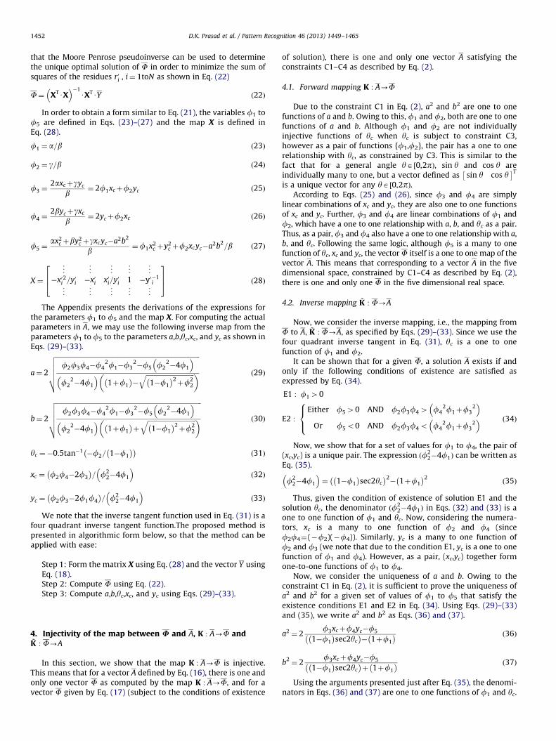
E13 P

1.27

1.

27

1.27

1.

26

1.25

1.

23

1.20

1.

18

1.15

1.

13

1.10

1.

08

1.06

1.

03

1.01

0.

99

d P 1.26

1.

26

1.26

1.

25

1.24

1.

22

1.20

. 1. Plot of error metrics for Experiment 7.1 (digital incomplete elliptic curves). (a) P

y and (c) Plot of (d–dP) for various values of Dy.

algorithm for any cluster of data. Ahn [18], Maini [14], and Liu[15] are iterative methods. Ahn [18] is the only method based onthe geometry of the ellipse. Maini [14] and Liu [15] are based onFitzgibbon [1] and aimed at improving the performance of ellipsedetection for special cases.

7.1. Digital incomplete/complete elliptic curves

We consider a family of elliptic curves given by bA[20,150],aA[b,150], aA ½0,pÞ, xc¼150, and yc¼150. In the range [y1,y1þDy],where y1 is randomly selected, a digital curve corresponding to theanalytical ellipse is generated. For various values of Dy, 1000 suchrandom curves are generated, corresponding to randomly chosenvalues of a,b,a, and y1. For these curves, the ellipses are fitted usingthe proposed method and the six methods used for comparison. Forthe fitted ellipses, ellipses that satisfy the following conditions areretained for further considerations:

The semi-major axis of a fitted ellipse should be less than 200.The ratio of the semi-minor to the semi-major axis (aspect

ratio) should be more than 0.1 (that is the eccentricity of theellipse should be less than 0.995).

The bias correction measures used in Harker [16] and Ahn [18]sometimes result in highly elliptic ellipses with huge values ofsemi-major axis. This unnecessarily tilts the performance metricsin favor of other methods since it can be easily concluded inpractice that the ellipses in the images may not be so large (of the

E14 P

5.23

5.

23

5.25

5.

25

5.27

5.

26

5.26

5.

26

5.25

5.

24

5.21

5.

19

5.16

5.

17

5.16

5.

17

1.17

1.

15

1.12

1.

10

1.07

1.

05

1.03

1.

01

0.99

lot of (E13–E13P) for various values of Dy, (b) Plot of (E14–E14P) for various values

D.K. Prasad et al. / Pattern Recognition 46 (2013) 1449–1465 1455

order of several powers of 10). Thus, condition (i) above wasincluded to compensate for this effect. The same bias correctionsmay alternatively keep the semi-major axis within reasonablevalue but push the value of the semi-minor axis to be close tozero. Condition (ii) above compensates for this effect.

The following performance parameters are plotted for each ofthe methods for the various values of Dy:

1.

Fig(b)

The mean of the error metric E13 as proposed by Rosin in [4].

2. The mean of the error metric E14 as proposed by Rosin in [12]. 3. The mean of the distances d¼

PNi ¼ 1 di=N of the pixels from

the fitted ellipse.

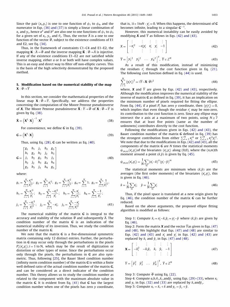
4. Total number of detected ellipses Etotal. 5. Recall: Recall¼ EOZ0:8=1000, where EOZ0.8 is the number of

detected ellipses that have overlap ratios O (given by Jaccardindex [26]) more than or equal to 0.8 with the correspondingactual ellipses).

6.

Precision: Precision¼ EOZ0:8=Etotal.

In the above, recall and precision are defined in Eqs. (49) and(50) below.

Precision¼number of true positive elliptic hypotheses

total number of elliptic hypothesesð49Þ

Recall¼number of true positive elliptic hypotheses

number of actual ellipsesð50Þ

The true positive ellipses in Eqs. (49) and (50) are defined usingthe overlap ratio O for ellipses as defined in [27]. We note thatthe first three are error metrics and the lower values of theseparameters are indicator of better fitting. On the other hand, the

. 2. Ellipse detection characteristics for Experiment 7.1 (digital incomplete ellipti

Plot of recall for various values of Dy and (c) Plot of precision for various values of

remaining three are related to the ellipse detection characteristics.The results are plotted in Fig. 1 (error metrics) and Fig. 2 (ellipsedetection characteristics). For a better representation of the data inFig. 1, we plotted the parameters E13, E14, and d with respect to theproposed data, i.e., we plot (E13�E13P), (E14�E14P), and (d�dP),where the subscript P denotes the proposed method. The values ofE13P, E14P, and dP are listed in the parts (a), (b), (c) of Fig. 1, respect-ively. The results in Fig. 1 show that the proposed method has thelowest values of the error metrics E13, E14, and d for all the values ofDy, while Ahn [18] and Harker [16] are the closest competitors.

Fig. 2 shows the total detected ellipses (Fig. 2(a)), recall (Fig. 2(b)),and precision (Fig. 2(c)) for various values of Dy. It is seen that theproposed method has successfully detected all the ellipses for allvalues of Dy except for Dy¼1351, for which the proposed methoddetected 982 ellipses out of 1000. While Chaudhri [19], Maini [14],and Liu [15] detected close to 1000 ellipses for each value of Dy, theirrecall and precision values are very poor. This is understandablebecause while Chaudhri [19] is an ellipse fitting algorithm that fitsellipses on any given cluster of points, it is not selective for ellipticshapes.

On the other hand, Liu [15] and Maini [14] are marginalimprovements of Fitzgibbon [1] which in most cases perform verysimilar to Fitzgibbon. Although Harker [16] detected close to 1000ellipses for each value of Dy, it has poor recall and precision ascompared to the proposed method and Ahn [18]. Although Ahn [18]has good precision (very close to the proposed method and themaximum value 1), it performed poorer than the proposed methodfor recall and significantly poorer than the proposed method interms of total detections. The total number of detected ellipses islow for Ahn [18] because it uses two nested non-linear iterativeoptimization processes and it is easy for Ahn [18] to eithermisconverge to a local minimum or to become non-convergent.On the other hand, the use of non-linear iterative optimization

c curves). (a) Plot of total number of detected ellipses for various values of Dy,

Dy.

D.K. Prasad et al. / Pattern Recognition 46 (2013) 1449–14651456

based on geometric principles helped Ahn [18] to be very precise ifit converges to the global minimum.

For illustration, we present an example of a digitized ellipsewith partial data corresponding to Dy¼1401 in Fig. 3. We notethat Ahn [18] does not detect the ellipse due to misconvergence,Fitzgibbon [1] and Liu [15] does not generate an ellipse thatsatisfies the conditions (i) and (ii) in Section 7.1, Maini [14] fits anellipse that is quite different from the actual ellipse, Harker [16]generates an ellipse similar (but not exactly matching) to theactual ellipse, Chaudhri [19] fitted an inaccurate ellipse, and onlythe proposed method managed to successfully detect the ellipsethat is very close to the actual ellipse from the partial digitalellipse data given as its input.

The results demonstrate good applicability of the proposedmethod for detecting elliptic shapes from digital images. Thus, theproposed method should be effective for applications that requiredetection of elliptic shapes from digital images. Since digitalimages are ubiquitous in today’s world and several natural and

Fig. 3. An example of digital incomplete elliptic curve (Experiment 7.1) and the result o

fitted ellipses are shown in thick (red) curves. (For interpretation of the references to c

E13 P

0.37

0.38

0.41

0.46

0.52

0.59

0.67

0.77

0.88

1.02

d P

0.37

0.39

0.42

0.46

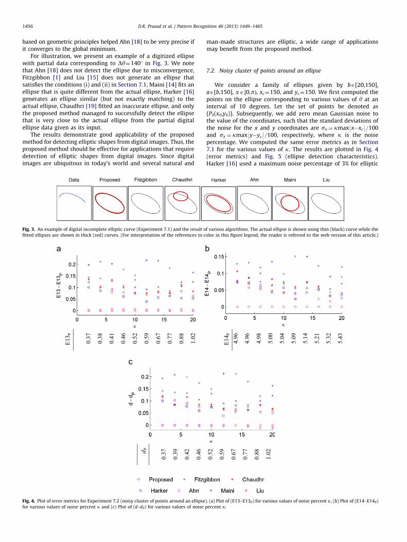
Fig. 4. Plot of error metrics for Experiment 7.2 (noisy cluster of points around an ellipse

for various values of noise percent k and (c) Plot of (d–dP) for various values of noise

man-made structures are elliptic, a wide range of applicationsmay benefit from the proposed method.

7.2. Noisy cluster of points around an ellipse

We consider a family of ellipses given by bA[20,150],aA[b,150], aA ½0,pÞ, xc¼150, and yc¼150. We first computed thepoints on the ellipse corresponding to various values of y at aninterval of 10 degrees. Let the set of points be denoted as{Py(xy,yy)}. Subsequently, we add zero mean Gaussian noise tothe value of the coordinates, such that the standard deviations ofthe noise for the x and y coordinates are sx ¼ kmax9x�xc9=100and sy ¼ kmax9y�yc9=100, respectively, where k is the noisepercentage. We computed the same error metrics as in Section7.1 for the various values of k. The results are plotted in Fig. 4(error metrics) and Fig. 5 (ellipse detection characteristics).Harker [16] used a maximum noise percentage of 3% for elliptic

f various algorithms. The actual ellipse is shown using thin (black) curve while the

olor in this figure legend, the reader is referred to the web version of this article.)

E14 P

4.96

4.96

4.98

5.00

5.04

5.09

5.14

5.21

5.32

5.43

0.52

0.59

0.67

0.77

0.88

1.02

). (a) Plot of (E13–E13P) for various values of noise percent k, (b) Plot of (E14–E14P)

percent k.

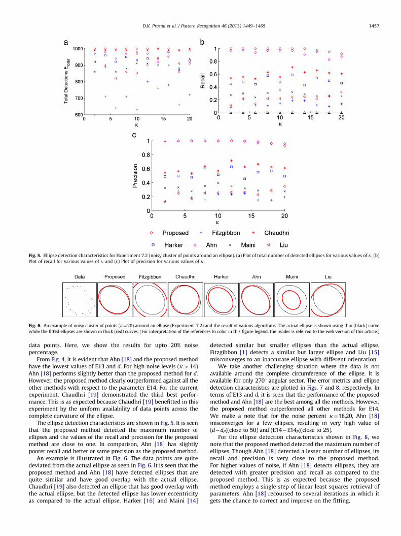
Fig. 5. Ellipse detection characteristics for Experiment 7.2 (noisy cluster of points around an ellipse). (a) Plot of total number of detected ellipses for various values of k, (b)

Plot of recall for various values of k and (c) Plot of precision for various values of k.

Fig. 6. An example of noisy cluster of points (k¼20) around an ellipse (Experiment 7.2) and the result of various algorithms. The actual ellipse is shown using thin (black) curve

while the fitted ellipses are shown in thick (red) curves. (For interpretation of the references to color in this figure legend, the reader is referred to the web version of this article.)

D.K. Prasad et al. / Pattern Recognition 46 (2013) 1449–1465 1457

data points. Here, we show the results for upto 20% noisepercentage.

From Fig. 4, it is evident that Ahn [18] and the proposed methodhave the lowest values of E13 and d. For high noise levels (k414)Ahn [18] performs slightly better than the proposed method for d.However, the proposed method clearly outperformed against all theother methods with respect to the parameter E14. For the currentexperiment, Chaudhri [19] demonstrated the third best perfor-mance. This is as expected because Chaudhri [19] benefitted in thisexperiment by the uniform availability of data points across thecomplete curvature of the ellipse.

The ellipse detection characteristics are shown in Fig. 5. It is seenthat the proposed method detected the maximum number ofellipses and the values of the recall and precision for the proposedmethod are close to one. In comparison, Ahn [18] has slightlypoorer recall and better or same precision as the proposed method.

An example is illustrated in Fig. 6. The data points are quitedeviated from the actual ellipse as seen in Fig. 6. It is seen that theproposed method and Ahn [18] have detected ellipses that arequite similar and have good overlap with the actual ellipse.Chaudhri [19] also detected an ellipse that has good overlap withthe actual ellipse, but the detected ellipse has lower eccentricityas compared to the actual ellipse. Harker [16] and Maini [14]

detected similar but smaller ellipses than the actual ellipse.Fitzgibbon [1] detects a similar but larger ellipse and Liu [15]misconverges to an inaccurate ellipse with different orientation.

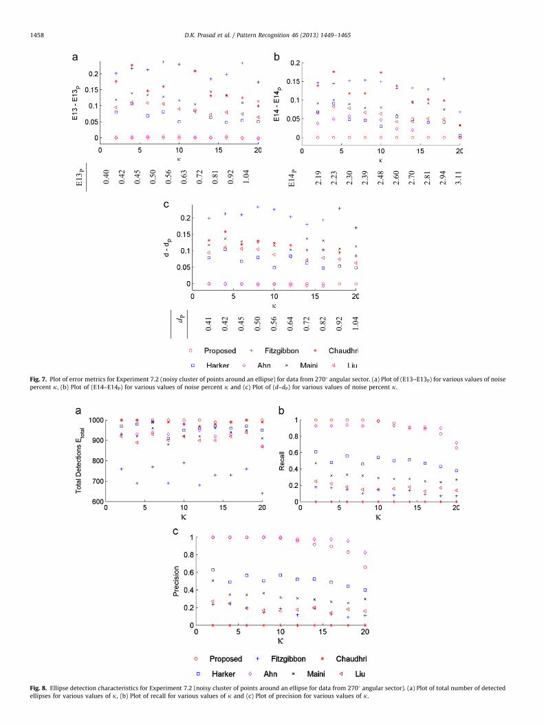
We take another challenging situation where the data is notavailable around the complete circumference of the ellipse. It isavailable for only 2701 angular sector. The error metrics and ellipsedetection characteristics are plotted in Figs. 7 and 8, respectively. Interms of E13 and d, it is seen that the performance of the proposedmethod and Ahn [18] are the best among all the methods. However,the proposed method outperformed all other methods for E14.We make a note that for the noise percent k¼18,20, Ahn [18]misconverges for a few ellipses, resulting in very high value of(d�dP)(close to 50) and (E14�E14P)(close to 25).

For the ellipse detection characteristics shown in Fig. 8, wenote that the proposed method detected the maximum number ofellipses. Though Ahn [18] detected a lesser number of ellipses, itsrecall and precision is very close to the proposed method.For higher values of noise, if Ahn [18] detects ellipses, they aredetected with greater precision and recall as compared to theproposed method. This is as expected because the proposedmethod employs a single step of linear least squares retrieval ofparameters, Ahn [18] recoursed to several iterations in which itgets the chance to correct and improve on the fitting.

E13 P

0.40

0.42

0.45

0.50

0.56

0.63

0.72

0.81

0.92

1.04

E14 P

2.19

2.23

2.30

2.39

2.48

2.60

2.70

2.81

2.94

3.11

d P

0.41

0.42

0.45

0.50

0.56

0.64

0.72

0.82

0.92

1.04

Fig. 7. Plot of error metrics for Experiment 7.2 (noisy cluster of points around an ellipse) for data from 2701 angular sector. (a) Plot of (E13–E13P) for various values of noise

percent k, (b) Plot of (E14–E14P) for various values of noise percent k and (c) Plot of (d–dP) for various values of noise percent k.

Fig. 8. Ellipse detection characteristics for Experiment 7.2 (noisy cluster of points around an ellipse for data from 2701 angular sector). (a) Plot of total number of detected

ellipses for various values of k, (b) Plot of recall for various values of k and (c) Plot of precision for various values of k.

D.K. Prasad et al. / Pattern Recognition 46 (2013) 1449–14651458

D.K. Prasad et al. / Pattern Recognition 46 (2013) 1449–1465 1459

An example with 2701 angular sector data and k¼20 isillustrated in Fig. 9. It is noted that the ellipse fitted by the proposedmethod is closest to the actual ellipse, followed by Ahn [18].Fitzgibbon [1] fitted to a very small ellipse, Chaudhri [19], Harker[16], Maini [14], and Liu [15] detected the ellipse with greateroverlap. Furthermore, these are not close to the actual ellipse.

Noise is often present in most practical scenarios. The effect ismore prominently seen in astronomical and medical data wherethe images often have clusters of points that are close to elliptic

Fig. 9. An example of noisy cluster of points (k¼20) around an ellipse (Experiment 7

shown using thin (black) curve while the fitted ellipses are shown in thick (red) curve

referred to the web version of this article.)

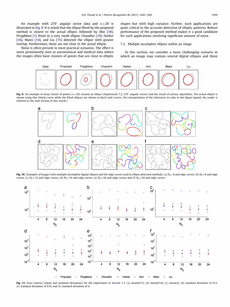
Fig. 10. Examples of images with multiple incomplete digital ellipses and the edge curv

curves, (c) NE¼12 and edge curves, (d) NE¼16 and edge curves, (e) NE¼20 and edge c

Fig. 11. Error metrics (mean and standard deviations) for the experiment in Section

(e) standard deviation of E14, and (f) standard deviation of d.

shapes but with high variance. Further, such applications arequite critical to the accurate detection of elliptic patterns. Robustperformance of the proposed method makes it a good candidatefor such applications involving significant amount of noise.

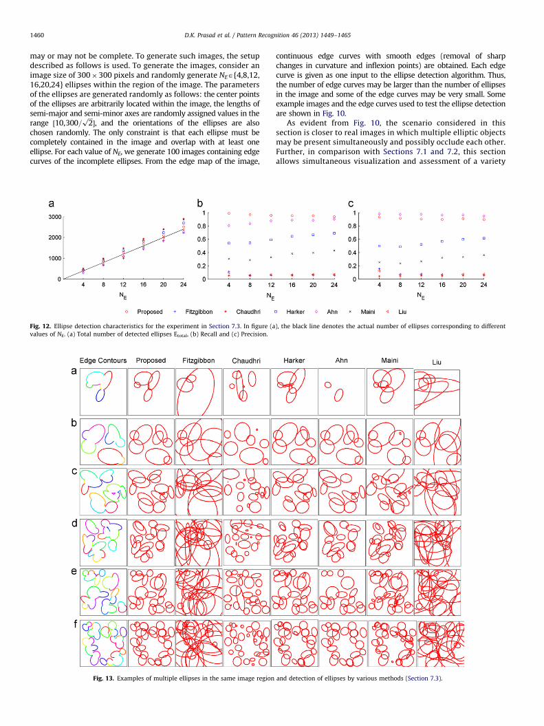
7.3. Multiple incomplete ellipses within an image

In this section, we consider a more challenging scenario inwhich an image may contain several digital ellipses and these

.2, 2701 angular sector) and the result of various algorithms. The actual ellipse is

s. (For interpretation of the references to color in this figure legend, the reader is

es used in ellipse detection methods. (a) NE¼4 and edge curves, (b) NE¼8 and edge

urves and (f) NE¼24 and edge curves.

7.3. (a) mean(E13), (b) mean(E14), (c) mean(d), (d) standard deviation of E13,

D.K. Prasad et al. / Pattern Recognition 46 (2013) 1449–14651460

may or may not be complete. To generate such images, the setupdescribed as follows is used. To generate the images, consider animage size of 300�300 pixels and randomly generate NEA{4,8,12,16,20,24} ellipses within the region of the image. The parametersof the ellipses are generated randomly as follows: the center pointsof the ellipses are arbitrarily located within the image, the lengths ofsemi-major and semi-minor axes are randomly assigned values in therange ½10,300=

ffiffiffi2p�, and the orientations of the ellipses are also

chosen randomly. The only constraint is that each ellipse must becompletely contained in the image and overlap with at least oneellipse. For each value of NE, we generate 100 images containing edgecurves of the incomplete ellipses. From the edge map of the image,

Fig. 12. Ellipse detection characteristics for the experiment in Section 7.3. In figure (a

values of NE. (a) Total number of detected ellipses Etotal, (b) Recall and (c) Precision.

Fig. 13. Examples of multiple ellipses in the same image region

continuous edge curves with smooth edges (removal of sharpchanges in curvature and inflexion points) are obtained. Each edgecurve is given as one input to the ellipse detection algorithm. Thus,the number of edge curves may be larger than the number of ellipsesin the image and some of the edge curves may be very small. Someexample images and the edge curves used to test the ellipse detectionare shown in Fig. 10.

As evident from Fig. 10, the scenario considered in thissection is closer to real images in which multiple elliptic objectsmay be present simultaneously and possibly occlude each other.Further, in comparison with Sections 7.1 and 7.2, this sectionallows simultaneous visualization and assessment of a variety

), the black line denotes the actual number of ellipses corresponding to different

and detection of ellipses by various methods (Section 7.3).

D.K. Prasad et al. / Pattern Recognition 46 (2013) 1449–1465 1461

of scenarios—very small fragments to large fragments, largeellipses to small ellipses, ellipses with high and low eccentricity,etc, which is also encountered in real world scenario.

It is highlighted that none of the methods, including theproposed method, group the incomplete edges potentially belong-ing to the same ellipse. Each method, including the proposedmethod, has exactly the same input—the coordinates of the pixelscorresponding to one edge curve only, i.e., one continuous curverepresented by a single color in Figs. 10 and 13 (second column).Thus, in one execution, the methods are in fact unaware of theexistence of other partial curves.

Since there are several ellipses and edge curves in each image,the standard deviation of the error metrics is also considered.Thus, for this experiment, we plot the mean values of the errormetrics E13, E14, and d (Fig. 11(a)–(c)), as well as their standarddeviations Fig. 11(d)–(f) in Fig. 11.

It is evident that the proposed method outperformed the restof the methods in terms of E13 and d, while it performed similarto or better than most methods in terms of E14. It is notable thatAhn [18] has significantly high mean values for all three errormetrics. This is because the misconvergence for one of the edgecurves in the image results in very high mean value of the errormetrics although the error metrics may have small value for the other

Fig. 14. Performance of ellipse fitting methods for analytical non-elliptic conics of Sect

detected ellipses and (b) an example and detected ellipses.

Fig. 15. Performance of ellipse fitting methods for digital non-elliptic conics of Sectio

detected ellipses and (b) an example and detected ellipses.

edge curves. This is also evident from the standard deviation dataplotted in Fig. 11(d)–(f), where it is seen than Ahn [18] has very highvalue for standard deviation as well. Similar effect happens with lessfrequency for Harker [16] as well, occasionally resulting in high meanand standard deviations (for example, see the data of Harker [16] forNE¼12 and NE¼24 in Fig. 11(b), (e)).

The ellipse detection characteristics are plotted in Fig. 12. Thenumber of ellipses detected by the proposed method is alwaysclose to the actual number of ellipses. The recall of the proposedmethod is the highest among all the methods and is close to onefor all values of NE. However, the precision of the proposedmethod is slightly poorer than the Ahn [18]. This is because thetotal number of ellipses detected by the proposed method isslightly higher than the actual number of ellipses for all values ofNE as the number of input curves to the methods might be greaterthan or equal to the total number of ellipses. Ahn [18] has aslightly poor recall ratio since the number of ellipses detected byAhn [18] is less than the number of actual ellipses. However,Ahn’s method detected the ellipses with slightly better precisionthan the proposed method. After the proposed method and Ahn’smethod, the next best performance is demonstrated by Harker[16]. We provide some examples in Fig. 13 to illustrate the ellipsedetection results in actual images.

ion 7.4 (the curves in black thin line denote the actual conics). (a) total number of

n 7.4 (the curves in black thin line denote the actual conics). (a) total number of

D.K. Prasad et al. / Pattern Recognition 46 (2013) 1449–14651462

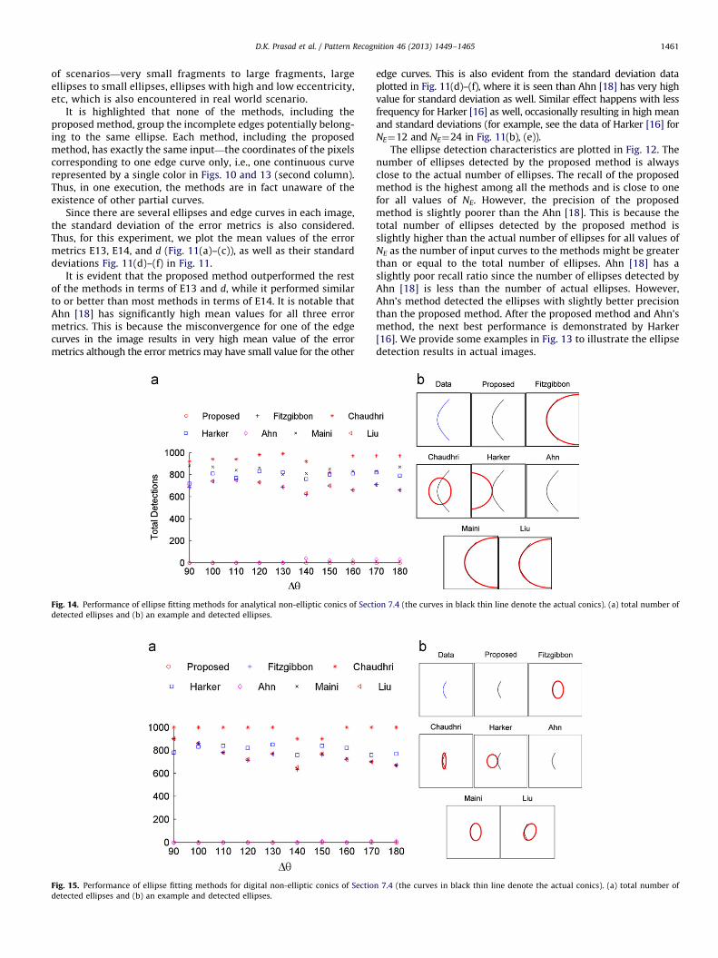
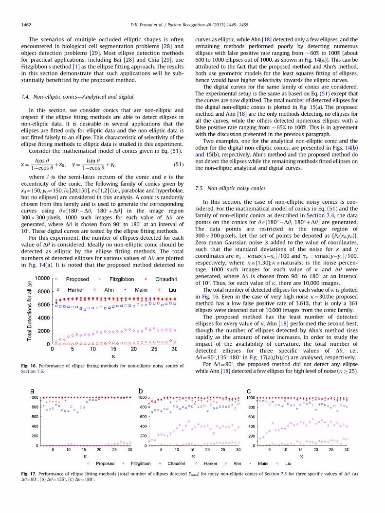
The scenarios of multiple occluded elliptic shapes is oftenencountered in biological cell segmentation problems [28] andobject detection problems [29]. Most ellipse detection methodsfor practical applications, including Bai [28] and Chia [29], useFitzgibbon’s method [1] as the ellipse fitting approach. The resultsin this section demonstrate that such applications will be sub-stantially benefitted by the proposed method.

7.4. Non-elliptic conics—Analytical and digital

In this section, we consider conics that are non-elliptic andinspect if the ellipse fitting methods are able to detect ellipses innon-elliptic data. It is desirable in several applications that theellipses are fitted only for elliptic data and the non-elliptic data isnot fitted falsely to an ellipse. This characteristic of selectivity of theellipse fitting methods to elliptic data is studied in this experiment.

Consider the mathematical model of conics given in Eq. (51).

x¼lcos y

1�ecos yþx0; y¼

lsin y1�ecos y

þy0 ð51Þ

where l is the semi-latus rectum of the conic and e is theeccentricity of the conic. The following family of conics given byx0¼150, y0¼150, lA[20,150], eA[1,2] (i.e., parabolae and hyperbolae,but no ellipses) are considered in this analysis. A conic is randomlychosen from this family and is used to generate the correspondingcurves using yA[1801�Dy, 1801þDy] in the image region300�300 pixels. 1000 such images for each value of Dy aregenerated, where Dy is chosen from 901 to 1801 at an interval of101. These digital curves are tested by the ellipse fitting methods.

For this experiment, the number of ellipses detected for eachvalue of Dy is considered. Ideally no non-elliptic conic should bedetected as elliptic by the ellipse fitting methods. The totalnumbers of detected ellipses for various values of Dy are plottedin Fig. 14(a). It is noted that the proposed method detected no

Fig. 16. Performance of ellipse fitting methods for non-elliptic noisy conics of

Section 7.5.

Fig. 17. Performance of ellipse fitting methods (total number of ellipses detected Eto

Dy¼901, (b) Dy¼1351, (c) Dy¼1801.

curves as elliptic, while Ahn [18] detected only a few ellipses, and theremaining methods performed poorly by detecting numerousellipses with false positive rate ranging from �60% to 100% (about600 to 1000 ellipses out of 1000, as shown in Fig. 14(a)). This can beattributed to the fact that the proposed method and Ahn’s method,both use geometric models for the least squares fitting of ellipses,hence would have higher selectivity towards the elliptic curves.

The digital curves for the same family of conics are considered.The experimental setup is the same as based on Eq. (51) except thatthe curves are now digitized. The total number of detected ellipses forthe digital non-elliptic conics is plotted in Fig. 15(a). The proposedmethod and Ahn [18] are the only methods detecting no ellipses forall the curves, while the others detected numerous ellipses with afalse positive rate ranging from �65% to 100%. This is in agreementwith the discussion presented in the previous paragraph.

Two examples, one for the analytical non-elliptic conic and theother for the digital non-elliptic conics, are presented in Figs. 14(b)and 15(b), respectively. Ahn’s method and the proposed method donot detect the ellipses while the remaining methods fitted ellipses onthe non-elliptic analytical and digital curves.

7.5. Non-elliptic noisy conics

In this section, the case of non-elliptic noisy conics is con-sidered. For the mathematical model of conics in Eq. (51) and thefamily of non-elliptic conics as described in Section 7.4, the datapoints on the conics for yA[1801�Dy, 1801þDy] are generated.The data points are restricted in the image region of300�300 pixels. Let the set of points be denoted as {Py(xy,yy)}.Zero mean Gaussian noise is added to the value of coordinates,such that the standard deviations of the noise for x and y

coordinates are sx ¼ kmax9x�xc9=100 and sy ¼ kmax9y�yc9=100,respectively, where kA ½1,30�;kAnaturals; is the noise percen-tage. 1000 such images for each value of k and Dy weregenerated, where Dy is chosen from 901 to 1801 at an intervalof 101. Thus, for each value of k, there are 10,000 images.

The total number of detected ellipses for each value of k is plottedin Fig. 16. Even in the case of very high noise k¼30,the proposedmethod has a low false positive rate of 3.61%, that is only a 361ellipses were detected out of 10,000 images from the conic family.

The proposed method has the least number of detectedellipses for every value of k. Ahn [18] performed the second best,though the number of ellipses detected by Ahn’s method risesrapidly as the amount of noise increases. In order to study theimpact of the availability of curvature, the total number ofdetected ellipses for three specific values of Dy, i.e.,Dy¼901,1351,1801 in Fig. 17(a),(b),(c) are analysed, respectively.

For Dy¼901, the proposed method did not detect any ellipsewhile Ahn [18] detected a few ellipses for high level of noise (kZ25).

tal) for noisy non-elliptic conics of Section 7.5 for three specific values of Dy. (a)

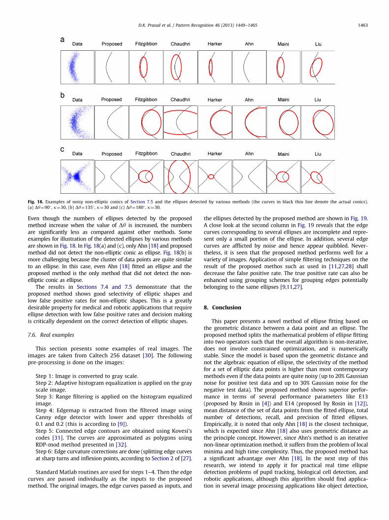
Fig. 18. Examples of noisy non-elliptic conics of Section 7.5 and the ellipses detected by various methods (the curves in black thin line denote the actual conics).

(a) Dy¼901, k¼30, (b) Dy¼1351, k¼30 and (c) Dy¼1801, k¼30.

D.K. Prasad et al. / Pattern Recognition 46 (2013) 1449–1465 1463

Even though the numbers of ellipses detected by the proposedmethod increase when the value of Dy is increased, the numbersare significantly less as compared against other methods. Someexamples for illustration of the detected ellipses by various methodsare shown in Fig. 18. In Fig. 18(a) and (c), only Ahn [18] and proposedmethod did not detect the non-elliptic conic as ellipse. Fig. 18(b) ismore challenging because the cluster of data points are quite similarto an ellipse. In this case, even Ahn [18] fitted an ellipse and theproposed method is the only method that did not detect the non-elliptic conic as ellipse.

The results in Sections 7.4 and 7.5 demonstrate that theproposed method shows good selectivity of elliptic shapes andlow false positive rates for non-elliptic shapes. This is a greatlydesirable property for medical and robotic applications that requireellipse detection with low false positive rates and decision makingis critically dependent on the correct detection of elliptic shapes.

7.6. Real examples

This section presents some examples of real images. Theimages are taken from Caltech 256 dataset [30]. The followingpre-processing is done on the images:

Step 1: Image is converted to gray scale.Step 2: Adaptive histogram equalization is applied on the grayscale image.Step 3: Range filtering is applied on the histogram equalizedimage.Step 4: Edgemap is extracted from the filtered image usingCanny edge detector with lower and upper thresholds of0.1 and 0.2 (this is according to [9]).Step 5: Connected edge contours are obtained using Kovesi’scodes [31]. The curves are approximated as polygons usingRDP-mod method presented in [32].Step 6: Edge curvature corrections are done (splitting edge curvesat sharp turns and inflexion points, according to Section 2 of [27].

Standard Matlab routines are used for steps 1–4. Then the edgecurves are passed individually as the inputs to the proposedmethod. The original images, the edge curves passed as inputs, and

the ellipses detected by the proposed method are shown in Fig. 19.A close look at the second column in Fig. 19 reveals that the edgecurves corresponding to several ellipses are incomplete and repre-sent only a small portion of the ellipse. In addition, several edgecurves are afflicted by noise and hence appear quibbled. Never-theless, it is seen that the proposed method performs well for avariety of images. Application of simple filtering techniques on theresult of the proposed methos such as used in [11,27,28] shalldecrease the false positive rate. The true positive rate can also beenhanced using grouping schemes for grouping edges potentiallybelonging to the same ellipses [9,11,27].

8. Conclusion

This paper presents a novel method of ellipse fitting based onthe geometric distance between a data point and an ellipse. Theproposed method splits the mathematical problem of ellipse fittinginto two operators such that the overall algorithm is non-iterative,does not involve constrained optimization, and is numericallystable. Since the model is based upon the geometric distance andnot the algebraic equation of ellipse, the selectivity of the methodfor a set of elliptic data points is higher than most contemporarymethods even if the data points are quite noisy (up to 20% Gaussiannoise for positive test data and up to 30% Gaussian noise for thenegative test data). The proposed method shows superior perfor-mance in terms of several performance parameters like E13(proposed by Rosin in [4]) and E14 (proposed by Rosin in [12]),mean distance of the set of data points from the fitted ellipse, totalnumber of detections, recall, and precision of fitted ellipses.Empirically, it is noted that only Ahn [18] is the closest technique,which is expected since Ahn [18] also uses geometric distance asthe principle concept. However, since Ahn’s method is an iterativenon-linear optimization method, it suffers from the problem of localminima and high time complexity. Thus, the proposed method hasa significant advantage over Ahn [18]. In the next step of thisresearch, we intend to apply it for practical real time ellipsedetection problems of pupil tracking, biological cell detection, androbotic applications, although this algorithm should find applica-tion in several image processing applications like object detection,

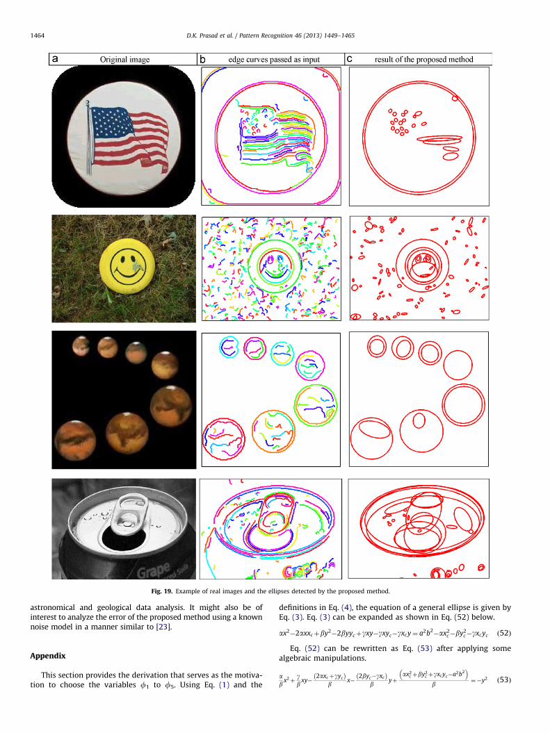
Fig. 19. Example of real images and the ellipses detected by the proposed method.

D.K. Prasad et al. / Pattern Recognition 46 (2013) 1449–14651464

astronomical and geological data analysis. It might also be ofinterest to analyze the error of the proposed method using a knownnoise model in a manner similar to [23].

Appendix

This section provides the derivation that serves as the motiva-tion to choose the variables f1 to f5. Using Eq. (1) and the

definitions in Eq. (4), the equation of a general ellipse is given byEq. (3). Eq. (3) can be expanded as shown in Eq. (52) below.

ax2�2axxcþby2�2byycþgxy�gxyc�gxcy¼ a2b2�ax2

c�by2c�gxcyc ð52Þ

Eq. (52) can be rewritten as Eq. (53) after applying somealgebraic manipulations.

ab

x2þgb

xy�2axcþgyc

� �b

x�2byc�gxc

� �b

yþax2

c þby2c þgxcyc�a2b2

� �b

¼�y2 ð53Þ

D.K. Prasad et al. / Pattern Recognition 46 (2013) 1449–1465 1465

Eq. (53) can be written in a matrix formulation after dividingboth the sides by (�y) as shown in Eq. (54) below.

� x2

y �x xy 1 � 1

y

h ia=bg=b

2axcþgyc

� �=b

2byc�gxc

� �=b

ax2c þby2

c þgxcyc�a2b2� �

=b

266666664

377777775¼ y½ � ð54Þ

As seen from Eq. (54), the definitions of the variables f1 to f5

should be given by Eqs. (23)–(27) and the matrix operator Xshould be given by (28).

References

[1] A. Fitzgibbon, M. Pilu, R.B. Fisher, Direct least square fitting of ellipses, IEEETransactions on Pattern Analysis and Machine Intelligence 21 (1999) 476–480.

[2] P.L. Rosin, A note on the least squares fitting of ellipses, Pattern RecognitionLetters 14 (1993) 799–808.

[3] P.L. Rosin, Ellipse fitting by accumulating five-point fits, Pattern RecognitionLetters 14 (1993) 661–669.

[4] P.L. Rosin, Analysing error of fit functions for ellipses, Pattern RecognitionLetters 17 (1996) 1461–1470.

[5] P.L. Rosin, Assessing error of fit functions for ellipses, Graphical Models andImage Processing 58 (1996) 494–502.

[6] D.K. Prasad, M.K.H. Leung, An ellipse detection method for real images,in: 25th International Conference of Image and Vision Computing NewZealand (IVCNZ 2010), Queenstown, New Zealand, 2010, pp. 1–8.

[7] D.K. Prasad, M.K.H. Leung, Error analysis of geometric ellipse detectionmethods due to quantization, in: Fourth Pacific-Rim Symposium on Imageand Video Technology (PSIVT 2010), Singapore, 2010, pp. 58–63.

[8] D.K. Prasad, M.K.H. Leung, A hybrid approach for ellipse detection in realimages, in: 2nd International Conference on Digital Image Processing,Singapore, 2010, pp. 75460I-6.

[9] F. Mai, Y.S. Hung, H. Zhong, W.F. Sze, A hierarchical approach for fast androbust ellipse extraction, Pattern Recognition 41 (2008) 2512–2524.

[10] A. Chia, S. Rahardja, D. Rajan, M.K.H. Leung, A split and merge based ellipsedetector with self-correcting capability, IEEE Transactions on Image Processing 20(2011) 1991–2006.

[11] E. Kim, M. Haseyama, H. Kitajima, Fast and robust ellipse extraction fromcomplicated images, in: Proceedings of the International Conference onInformation Technology and Applications, 2002, pp. 357–362.

[12] P.L. Rosin, Ellipse fitting using orthogonal hyperbolae and Stirling’s oval,Graphical Models and Image Processing 60 (1998) 209–213.

[13] P.L. Rosin, Evaluating Harker and O’Leary’s distance approximation for ellipsefitting, Pattern Recognition Letters 28 (2007) 1804–1807.

[14] E.S. Maini, Enhanced direct least square fitting of ellipses, InternationalJournal of Pattern Recognition and Artificial Intelligence 20 (2006)939–953.

[15] Z.Y. Liu, H. Qiao, Multiple ellipses detection in noisy environments:A hierarchical approach, Pattern Recognition 42 (2009) 2421–2433.

[16] M. Harker, P. O’Leary, P. Zsombor-Murray, Direct type-specific conic fitting

and eigenvalue bias correction, Image and Vision Computing 26 (2008)372–381.

[17] R. Halir, J. Flusser, Numerically stable direct least squares fitting of ellipses,in: Sixth International Conference in Central Europe on Computer Graphics

and Visualization, 1998, pp. 125–132.[18] S.J. Ahn, W. Rauh, H.J. Warnecke, Least-squares orthogonal distances fitting of

circle, sphere, ellipse, hyperbola, and parabola, Pattern Recognition 34 (2001)

2283–2303.[19] D. Chaudhuri, A simple least squares method for fitting of ellipses and circles

depends on border points of a two-tone image and their 3-D extensions,Pattern Recognition Letters 31 (2010) 818–829.

[20] D.K. Prasad, C. Quek, M.K.H. Leung, A precise ellipse fitting method for noisydata, in: International Conference on Image Analysis and Recognition (ICIAR

2012), Aveiro, Portugal, 2012, pp. 253–260.[21] D. Keren, D. Cooper, J. Subrahmonia, Describing complicated objects by

implicit polynomials, IEEE Transactions on Pattern Analysis and Machine

Intelligence 16 (1994) 38–53.[22] D. Keren, C. Gotsman, Fitting curves and surfaces with constrained implicit

polynomials, IEEE Transactions on Pattern Analysis and Machine Intelligence21 (1999) 31–41.

[23] M. Werman, D. Keren, A Bayesian method for fitting parametric andnonparametric models to noisy data, IEEE Transactions on Pattern Analysisand Machine Intelligence 23 (2001) 528–534.

[24] G. Taubin, Estimation of planar curves, surfaces, and nonplanar space curvesdefined by implicit equations with applications to edge and range image

segmentation, IEEE Transactions on Pattern Analysis and Machine Intelli-gence 13 (1991) 1115–1138.

[25] S.M. Rump, Structured perturbations and symmetric matrices, Linear Algebraand Its Applications 278 (1998) 121–132.

[26] P.N. Tan, M. Steinbach, V. Kumar, Introduction to data mining, PearsonAddison Wesley, 2006.

[27] D.K. Prasad, M.K.H. Leung, S.Y. Cho, Edge curvature and convexity basedellipse detection method, Pattern Recognition 45 (2012) 3204–3221.

[28] X. Bai, C. Sun, F. Zhou, Splitting touching cells based on concave points andellipse fitting, Pattern Recognition 42 (2009) 2434–2446.

[29] A.Y.-S. Chia, S. Rahardja, D. Rajan, M.K. Leung, Object recognition bydiscriminative combinations of line segments and ellipses, in: Proceedingsof the IEEE Conference on Computer Vision and Pattern Recognition, San

Francisco, USA, 2010, pp. 2225–2232.[30] G. Griffin, A. Holub, P. Perona, Caltech-256 object category database [/http://

authors.library.caltech.edu/7694S]. Available: /http://authors.library.caltech.edu/7694S.

[31] P.D. Kovesi, MATLAB and Octave Functions for Computer Vision and ImageProcessing (2000 ed.) [/http://www.csse.uwa.edu.au/~pk/Research/MatlabFns/index.htmlS].

[32] D.K. Prasad, M.K.H. Leung, C. Quek, S.-Y. Cho, A novel framework for makingdominant point detection methods non-parametric, Image and Vision Com-

puting 30 (2012) 843–859.

Dilip Kumar Prasad received the B.Tech degree in Computer Science and Engineering from Indian School of Mines, Dhanbad, India in 2003. He did his PhD in ComputerEngineering from Nanyang Technological University, Singapore. Currently, he is a research fellow at National University of Singapore, Singapore. He has 5 years ofindustrial experience with IBM, Mediatek, and Philips in the field of embedded systems. He has published over 25 internationally peer-reviewed research articles. Hiscurrent research interests include image processing, pattern recognition and discrete geometry.

Dr. Maylor K.H. Leung received the BSc degree in physics from the National Taiwan University in 1979, and the BSc, MSc and PhD degrees in computer science from theUniversity of Saskatchewan, Canada, in 1983, 1985 and 1992, respectively. Currently, Dr. Leung is a Professor with Faculty of Inform. & Comm. Tech., Universiti TunkuAbdul Rahman (Kampar), Malaysia. His research interest is in the area of Computer Vision, Pattern Recognition and Image Processing.

Dr. Chai Quek is currently in the School of Computer Engineering, Nanyang Technological University, Singapore since 1990. He received his Bachelor degree in Science andPh.D. degrees from the Heriot-Watt University (Edinburgh). His research interests include Neurocognitive informatics, Biomedical Engineering and Computational Finance.He has done significant research work in his research areas and published over 200 top quality international conference and journal papers. He has been often invited as aprogram committee member and reviewer for a number of premier conferences and journals, including IEEE TNN, TEvC etc. Dr. Quek is a senior member of IEEE. He is alsoa member of the IEEE Technical Committee on Computational Finance and Economics. He has constantly and successfully groomed several high caliber researchers who areawarded prestigious Singapore Millennium Foundation Scholarship and Fellowship, Lee Kuan Yew Fellowship and AnStar Scholarship.