JHEP05(2013)135

Published for SISSA by Springer

Received: May 1, 2013

Accepted: May 2, 2013

Published: May 27, 2013

Eliminating spurious poles from gauge-theoretic

amplitudes

Andrew Hodges

Mathematical Institute,

24-29 St Giles, Oxford OX1 3LB, U.K.

E-mail: hodges@maths.ox.ac.uk

Abstract: This note addresses the problem of spurious poles in gauge-theoretic scattering

amplitudes. New twistor coordinates for the momenta are introduced, based on the concept

of dual conformal invariance. The cancellation of spurious poles for a class of NMHV

amplitudes is greatly simplified in these coordinates. The poles are eliminated altogether

by defining a new type of twistor integral, dual to twistor diagrams as previously studied,

and considerably simpler. The geometric features indicate a supersymmetric extension

of the formalism at least to all NMHV amplitudes, allowing the dihedral symmetry of the

super-amplitude to be made manifest. More generally, the definition of ‘momentum-twistor’

coordinates suggests a powerful new approach to the study of scattering amplitudes.

Keywords: Supersymmetric gauge theory, Scattering Amplitudes

ArXiv ePrint: 0905.1473

c© SISSA 2013 doi:10.1007/JHEP05(2013)135

JHEP05(2013)135

Contents

1 The problem of spurious poles 1

1.1 The split-helicity 6-field NMHV amplitude 2

1.2 Super-amplitudes and dihedral symmetry 3

2 Dual conformal symmetry 4

2.1 Momentum-twistor coordinates 4

2.2 Translating the amplitude 9

3 New integrals in momentum-twistor space 9

3.1 Why spurious poles cancel: spurious boundaries 11

3.2 Generalisation to more than six fields 13

3.3 NMHV split-helicity amplitudes for seven fields 14

3.4 NMHV split-helicity amplitudes for n fields 15

4 Supersymmetric extension to all helicities 16

4.1 Polytopes with dihedral symmetry 18

4.2 The combinatorics of BCFW 19

4.3 Summary: super-amplitudes as super-volumes 20

5 Subsequent developments 20

1 The problem of spurious poles

In this note1 we tackle the problem which plagues the representation of all gauge-theoretic

scattering amplitudes except the MHV and MHV. The on-shell recursion relation due to

Britto, Cachazo, Feng and Witten [1], referred to as BCFW in what follows, has enormously

simplified the calculation of amplitudes in terms of momentum-space spinors. But it leaves

the results in the form of a sum of rational functions of momenta which, individually, have

singularities which are not present in the amplitude itself. These are the spurious poles.

We will start with the simplest example of this phenomenon.

1The original preprint can be read on arXiv:0905.1473v1. This paper differs from it principally in that

its section 5 on ‘Outlook’ has been replaced by a brief note on subsequent developments. Otherwise, apart

from minor corrections and typographical changes, the exposition remains unchanged. It is intended that

this will provide a useful elementary introduction to the momentum twistor coordinates and the polytope

description of amplitudes which were first proposed in this work.

– 1 –

JHEP05(2013)135

1.1 The split-helicity 6-field NMHV amplitude

We consider the (colour-stripped) amplitude A(1−2−3−4+5+6+). This has a special sim-

plicity because of the ‘split-helicity’ distribution of + and − helicities into just two sets

around the ring.

The BCFW recursion can readily be applied to evaluate the amplitude, but the result

obtained depends on the selection of the pivoting pair. Two quite different expressions

result, one in two terms and one in three:

[4|5 + 6|1〉3

[34][23]〈56〉〈61〉[2|3 + 4|5〉S234

+[6|1 + 2|3〉3

[61][12]〈34〉〈45〉[2|3 + 4|5〉S612

δ

( 6∑

i=1

pi

)

(1.1)

and

(S123)3

[12][23]〈45〉〈56〉[1|2 + 3|4〉[3|4 + 5|6〉

+〈12〉3[45]3

〈16〉[34][3|4 + 5|6〉[5|6 + 1|2〉S612

+〈23〉3[56]3

〈34〉[16][1|2 + 3|4〉[5|6 + 1|2〉S234

δ

( 6∑

i=1

pi

)

. (1.2)

It is far from obvious that these two representations of the amplitude are equiva-

lent. Their equality is guaranteed by the derivation of BCFW recursion from the Feyn-

man rules, but is difficult to show directly. Nor is it immediately apparent that the poles

[2|3+4|5〉, [1|2+3|4〉, [3|4+5|6〉, [5|6+1|2〉 are spurious, each of them cancelling, apparently

miraculously, when the terms are added. (It does of course follow from the equivalence of

the expressions that these poles must be spurious, but this does not suggest a natural way

of seeing the cancellations.) Taking another approach, it is straightforward to see from

the Feynman expansion that singularities can only arise from the vanishing of the scalar

invariants Sij , Sijk etc., and this gives another proof that any poles other than these must

be spurious. But again, such an argument depends on a lengthy sequence of algebraic

manipulations, involving the very gauge-dependent terms that the BCFW recursion has so

marvellously eliminated.

It is not difficult to see, in general terms, how such spurious singularities can arise.

A key ingredient of the BCFW recursion is the application of complex analysis on CP1

to produce an identity based on partial fractions. Such identities naturally give rise to

spurious poles. As an analogy, consider:

1

(z − v)(z − w)=

1

(v − w)

1

(z − v)+

1

(w − v)

1

(z − w). (1.3)

If v 6= w, this can be established by considering the behaviour of each side as an analytic

function of z. The agreement of the residues at z = v, z = w, and the regularity at z = ∞,

– 2 –

JHEP05(2013)135

suffice. But the identity has a spurious pole at v = w, where the residue calculus formula

fails to apply. The spurious poles in the amplitude likewise correspond to coincidences of

parameters. For instance, the vanishing of [1|2 + 3|4〉 implies that S23S1234 = S123S234.

Algebraic verification of the equivalence of these expressions is difficult because in ad-

dition to use of the spinor (Schouten) identity ǫABǫCD + ǫACǫDB + ǫADǫBC = 0, it calls

on repeated applications of the four constraints imposed by the δ-function. Field theo-

rists have generally chosen a spinor basis in which to express these constraints, then used

computer-supported algebra.

1.2 Super-amplitudes and dihedral symmetry

It is now well understood that super-symmetric extension eliminates the restriction on helic-

ities in the original BCFW recursion, and greatly increases its power. Arkani-Hamed, Cac-

hazo and Kaplan [2] have given an extensive account of the significance of this development

for physical theory. The concept of super-amplitude greatly simplifies scattering theory by

treating all helicity cases at once. In particular, as a function of n (super-)momenta pai the

super-amplitude has a simple symmetry: it must be invariant under i→ i+1 and i→ n−i.

Yet this simple dihedral symmetry is hidden in the (super-)BCFW expansion. The

difficulty of showing the equivalence of expressions (1.1) and (1.2) is just one aspect of

this larger problem. Their equality is just one super-component of a identity for six super-

fields, asserting a hidden D6 symmetry. This was identified as the hexagon identity by this

author in presenting an earlier version of super-BCFW recursion through the extension of

the twistor diagram formalism [3].

Arkani-Hamed et al. [4] gave the analogue of this formalism for split-signature the-

ory, whilst Mason and Skinner [6] also gave a parallel derivation. (The advantage of the

split-signature case is that the requisite integrations can be stated precisely, without the

difficulty of defining contours that pervades the Minkowski space theory. The disadvantage

is that it lacks the physical content of scattering theory as a process connecting past and

future.) This confluence has greatly stimulated fresh interest in the problems of the hid-

den dihedral symmetry and the spurious poles, because these combinatorial features are

essentially the same in split-signature theory as in Minkowski space.

The spurious poles are problematic from a practical computational point of view, as

well as presenting a long-standing difficulty in the theory. For more than six fields, the com-

plexity and asymmetry only increase. For the NMHV amplitude for n fields, a BCFW re-

cursion gives rise to (n−3)(n−4)/2 terms, each choice of pivots giving rise to a different sum

of terms. (For special helicity configurations, as with the split-helicity six-field case, some of

these terms vanish, giving a formula with fewer terms.) The general situation for tree-level

amplitudes is even more complex. For n fields the amplitudes require a total of (2n−6)!(n−3)!(n−2)!

terms. (This was noted in [3], as an aspect of the twistor diagram form of the BCFW re-

cursion; Arkani-Hamed et al. [4] make further interesting suggestions based on the Catalan

number that appears in this combinatorial formula.) Within this, the sector with n − r

fields of negative helicity and r of positive helicity accounts for (n−4)!(n−3)!(r−2)!(n−r−1)!(r−1)!(n−r−2)!

terms. It is, of course, a considerable triumph that explicit formulas for these terms can

– 3 –

JHEP05(2013)135

now be given, based on carrying out the BCFW recursion for n steps. But these statements

of the answers are no less complex than the recursion relation itself.

These formulas conceal the Dn dihedral symmetry of the n-field amplitudes. They

also conceal the identities which follow from the Dm dihedral symmetry of the m-field

amplitudes, where m < n, which can be used to put the n-field amplitudes in a more

symmetrical form. One of the advantages of the twistor diagram form of the super-BCFW

expansion [3, 5], is that it gives a graphical form to these identities. This is also noted and

exploited by Arkani-Hamed et al. [4].

Explicitly, the ‘square identity’, which expresses the D4 symmetry of the n = 4 super-

amplitude, is needed to get even the manifest D3 symmetry of the n = 6 NMHV ampli-

tudes. The D6 ‘hexagon identity’ can then be used to show the D4 symmetry of the n = 8

NNMHV amplitudes [3, 7]. The full D8 symmetry of these amplitudes then resides in a

formidable 40-term identity.2

Not all authors have found it important to focus upon these hidden symmetries. Mason

and Skinner [6], for instance, simply present one particular n = 8 NNMHV summation as

an application of their calculus, placing their emphasis on the super-conformal invariance of

the individual terms, as elegantly derived from super-twistor geometry. But Arkani-Hamed

has made a point of the idea that such summations fail to present important aspects of the

solution. His emphasis on the significance of the spurious poles has stimulated the present

enquiry. (He has also emphasised that the hidden part of the symmetry can also be seen as a

parity symmetry — invariance when the role of twistors and dual twistors is interchanged.)

Can twistor geometry go further in bringing out what is hidden, and so not just translating

BCFW but adding new content to the description of amplitudes? Yes, it can.

2 Dual conformal symmetry

In what follows we shall generally be considering sequences of n spinors, vectors, or twistors

with a cyclical property. We use throughout the natural convention in which the labelling

is modulo n, allowing the nth element of a sequence also to be called the 0th.

A first observation is that the equivalence of (1.1) and (1.2) should be seen as a five-

term identity for 12 independent complex spinors, subject to four holomorphic constraints,

as indicated by the δ-function. Imposing a reality condition on the momentum, so that the

spinors are complex conjugates, does not simplify the question.

2.1 Momentum-twistor coordinates

Nothing in the expressions (1.1), (1.2), suggests an immediate connection with twistors.

Nevertheless, the key step is to introduce new twistor-valued coordinates with which to

express the content of these momentum spinors. We shall call these momentum-twistors.

2The 2009 preprint commented that this 40-term identity had probably never been checked explicitly,

but the later analysis of Arkani-Hamed et al. [8] classified all such identities. The 2009 preprint also

commented here that twistor diagrams had not so far shown how to derive the identities without reference

to the Feynman theory. This is also achieved by the analysis of [8]. But these advances do not affect the

thrust of these remarks, viz. that it would be desirable to see such summations as flowing from a single

geometrical structure. Indeed, this aspiration is echoed in the concluding remarks of [8].

– 4 –

JHEP05(2013)135

Using Penrose’s original conventions for classical twistor geometry, twistors Zα are

written as (ωA, πA′), the spinors being referred to as ω- and π-parts of the twistor. A point

xa in complexified Minkowski space CM is said to lie on the α-plane of the twistor Zα, if

ωA = ixAA′

πA′ . Twistors with vanishing π-parts have no such finite xa, and correspond to

an α-plane in the null cone at infinity in the compactification of CM. If the skew two-index

twistor P [αQβ] does not vanish, it defines a projective line in twistor space; if πA′

P πQA′ 6= 0

then this corresponds to a finite point in CM. Dual twistor space is defined in the standard

sense of vector and projective spaces; dual twistors have the form (πA, ωA′

) and are, pro-

jectively, planes in twistor space. (It is often convenient to use the projective terms point,

line, and plane even when the twistors are given a scale.) The complex conjugate Zα is de-

fined as an element in dual twistor space, and the resulting (++−−) pseudo-norm ensures

that twistors represent the conformal group on (real, compactified) Minkowski space. It is

remarkable, however, how much structure is purely holomorphic, and exists independently

of this definition. (That our momentum-spinor identities are purely holomorphic is an

example of this.) In contrast, the mechanism for the breaking of conformal invariance, by

picking out the null cone at infinity, is an all-pervasive aspect of the application of twistor

theory to scattering amplitudes. It appears in twistor algebra through the special skew

two-index twistors Iαβ , Iαβ, which represent the vertex of the null cone at infinity.

The π-part of a twistor is obtained by transvecting it with Iαβ , as IαβZβ = (0, πA

′

).

A useful formula relating twistor and space-time geometry is that if Pα, Qα define a line in

projective twistor space, corresponding to a point xa in CM, whilst Rα, Sα similarly define

ya, then the displacement tensor

Dαβ =

IακǫκλµνPλQµR[νSσ]Iσβ

(IλµP λQµ)(IνσRνSσ)(2.1)

has only one non-vanishing component, namely (x− y)AB′

. Furthermore

(x− y)2 = −2ǫλµνσP

λQµRνSσ

(IλµP λQµ)(IνσRνSσ). (2.2)

In choosing these momentum-twistor coordinates we are motivated by the concept of region

space on which dual conformal symmetry is defined. This is an affine space in which the

external null momenta pai are defined as differences xai − xai−1, so that momentum con-

servation is expressed by xa0 = xan. The concept of region is only well-defined when the

momenta have a sequential structure, such as arises from the colour-ordering. It is worth

noting that dual conformal symmetry only holds for the colour-stripped amplitudes for the

planar Feynman graphs. Unlike the conformal symmetry in Minkowski space, it does not

characterise the entire physical theory, but has a secondary character.

The concept of region space, and of conformal symmetry in this space, has long played

an important role in the calculation of loop amplitudes for gauge theory. Recently, further

inspiring discoveries have been made about dual super-conformal symmetry [9–11], where,

again, it is the extension to the full N=4 gauge theory with loops that is the driving force.

In contrast, the discussion in this note is limited to tree-amplitudes, but the fact that

this symmetry has such a powerful role in the full theory is part of the motivation. Note

– 5 –

JHEP05(2013)135

x3

x4

x5

x6

x1

x2

p3 p4

p5

p6p1

p2

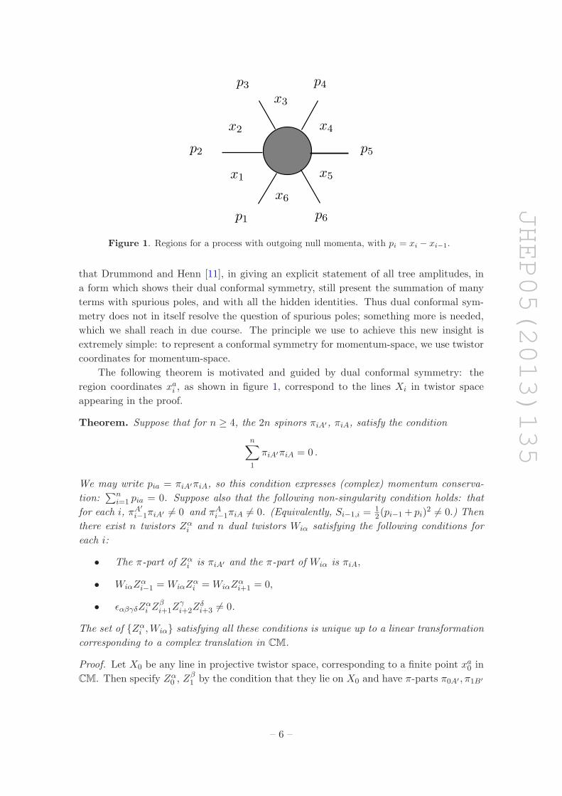
Figure 1. Regions for a process with outgoing null momenta, with pi = xi − xi−1.

that Drummond and Henn [11], in giving an explicit statement of all tree amplitudes, in

a form which shows their dual conformal symmetry, still present the summation of many

terms with spurious poles, and with all the hidden identities. Thus dual conformal sym-

metry does not in itself resolve the question of spurious poles; something more is needed,

which we shall reach in due course. The principle we use to achieve this new insight is

extremely simple: to represent a conformal symmetry for momentum-space, we use twistor

coordinates for momentum-space.

The following theorem is motivated and guided by dual conformal symmetry: the

region coordinates xai , as shown in figure 1, correspond to the lines Xi in twistor space

appearing in the proof.

Theorem. Suppose that for n ≥ 4, the 2n spinors πiA′, πiA, satisfy the condition

n∑

1

πiA′πiA = 0 .

We may write pia = πiA′πiA, so this condition expresses (complex) momentum conserva-

tion:∑n

i=1 pia = 0. Suppose also that the following non-singularity condition holds: that

for each i, πA′

i−1πiA′ 6= 0 and πAi−1πiA 6= 0. (Equivalently, Si−1,i =12(pi−1+ pi)

2 6= 0.) Then

there exist n twistors Zαi and n dual twistors Wiα satisfying the following conditions for

each i:

• The π-part of Zαi is πiA′ and the π-part of Wiα is πiA,

• WiαZαi−1 =WiαZ

αi =WiαZ

αi+1 = 0,

• ǫαβγδZαi Z

βi+1Z

γi+2Z

δi+3 6= 0.

The set of {Zαi ,Wiα} satisfying all these conditions is unique up to a linear transformation

corresponding to a complex translation in CM.

Proof. Let X0 be any line in projective twistor space, corresponding to a finite point xa0 in

CM. Then specify Zα0 , Z

β1 by the condition that they lie on X0 and have π-parts π0A′ , π1B′

– 6 –

JHEP05(2013)135

respectively. These points are well-defined and distinct, by the non-singularity condition.

Now consider the point xa0 + πA1 πA′

1 , with a corresponding line X1 in twistor space. This

line is not coincident with P0, since π1Aπ1A′ 6= 0, and it also represents a finite point in

CM. Note that Zβ1 lies on X1. Define Zγ

2 by it lying on X1, and having π-part π2C′ .

Clearly Zα0 , Z

β1 , Z

γ2 define a plane. Continue in the same way, so that line Xk corresponds

to the point xa0 +∑k

i=1 πAi π

A′

i . Eventually we define a twistor Zαn−1 by this means. Now

define Xn by the same method, and it corresponds to the point xa0 +∑n

i=1 πAi π

A′

i . By the

hypothesis on the 2n given spinors, this is just xa0. Hence Xn = X0 and the definition of

the n twistors Zαi is complete and consistent.

The dual twistors Wiα are now defined by the planes containing consecutive triples of

the Xi. Explicitly, including the scale:

Wiα =ǫαβγδZ

βi−1Z

γi Z

δi+1

(IλµZλi−1Z

µi ) (IνσZ

νi Z

σi+1)

. (2.3)

This is the all-important formula which allows momentum-space amplitudes to be expressed

in momentum-twistors. By construction, the Wiα satisfy all the orthogonality properties

stated. To check that the π-part of Wiα is πiA, apply the formula (2.1) to the lines Xi−1

and Xi. We obtain for the displacement tensor

Dαβ =

IακǫκγδθZγi−1Z

δi Z

[θi Z

φ]i+iIφβ

(IλµZλi−1Z

µi ) (IνσZ

νi Z

σi+1)

= IφβZφi

IακǫκγδθZγi−1Z

δi Z

θi+1

(IλµZλi−1Z

µi ) (IνσZ

νi Z

σi+1)

= (IφβZφi )(I

ακWiκ) . (2.4)

But this must agree with the displacement vector πA′

i πAi , so the the π-part of Wiα is πiA,

as required.

As an alternative to this geometrical proof, we may state algebraic formulas for the

Zαi and Wiα as follows:

Zαk =

(

iπkB′

(

xAB′

0 +

k−1∑

i=1

πAi πB′

i

)

, πkA′

)

,

Wkα =

(

πkA,−iπkB

(

xBA′

0 +k−1∑

i=1

πBi πA′

i

))

, (2.5)

and verify that all the conditions are satisfied. This formula brings out how each Zαi and

Wiα depends non-linearly on the 2n given momentum-spinors.

The line X0 was arbitrary. Choosing a different line is equivalent to a translation in

CM, equivalent to a volume-preserving linear transformation of the Zαi which preserves

Iαβ . We shall find that the Zαi appear only through the combinations IαβZ

αi−1Z

βi and

ǫαβγδZαi Z

βj Z

γkZ

δl , which are invariant under just this group of transformations.

For a proof of the uniqueness statement, suppose that Zαi andWiα are any solutions of

these equations. The conditions they satisfy imply the existence of distinct points xai , each

– 7 –

JHEP05(2013)135

null-separated from its neighbours, whence the Zαi must agree with the Zα

i as constructed

above. The uniqueness fails if the condition ǫαβγδZαi Z

βi+1Z

γi+2Z

δi+3 6= 0 is not imposed. If

it is violated, the xai need not be distinct. Let X0 be any line corresponding to a finite

point in CM; there exist points Zαi all on X0, and Wiα planes all containing X0, satisfying

all the other conditions.

The amplitudes are generally singular if any Si−1,i vanishes, so this exclusion does

not impede our ability to map momentum-space amplitudes into the new momentum-

twistor coordinates. In the reverse direction, we shall find that the non-vanishing of

ǫαβγδZαi Z

βi+1Z

γi+2Z

δi+3 is also a natural condition on the amplitudes. For the analysis of

infra-red divergences and soft limits, however, it may be profitable to scrutinise in finer

detail the way that the correspondence between momenta and the Zαi fails to hold in this

singular region.

Having excluded this singular region, the Wiα are completely defined by the Zαi , which

are themselves defined, up to the freedom stated, by the 2n spinors. So we have a good

encoding of the given 2n spinors in terms of n twistors — a coding which absorbs the

momentum-conservation condition. The π-parts of dual twistors are replaced by ω-parts

of twistors (or, equally well, the other way round). The 4-vector condition implied by the

sum∑n

1 πA′

i πiA = 0 has been converted into the 4-vector freedom in the choice of the

Zαi . This is just the same freedom as in the ‘region space’ of xa on which dual conformal

symmetry is defined, with the slight difference that in the twistor geometry there is no

reason to consider the momenta as being real.

It is convenient to introduce some notation. We have already used the convention of

angle-brackets and square brackets for spinor products, thus

〈12〉 = πA′

1 π2A′ = IαβZα1 Z

β2 ,

[12] = πA1 π2A = IαβW1αW2β . (2.6)

Now define also the conformally invariant (actually SL4C invariant) objects

〈1234〉 = ǫαβγδZα1 Z

β2Z

γ3Z

δ4 ,

[1234] = ǫαβγδW1αW2βW3γW4δ . (2.7)

Then from applying formula (2.3),

[12] =〈0123〉

〈01〉〈12〉〈23〉, (2.8)

s12 =1

2(p1 + p2)

2 = 〈12〉[12] =1

2(x0 − x2)

2 =〈0123〉

〈01〉〈23〉. (2.9)

The property of the amplitudes, essential to dual conformal invariance, is that the momenta

only enter through sums of consecutive momenta (consecutive, that is, in the ordering de-

fined by the colour-trace). In the momentum-twistor representation, this is reflected in the

simplicity of the further invariants

S123 =1

2(x0 − x3)

2 =〈0134〉

〈01〉〈34〉, S1234 =

1

2(x0 − x4)

2 =〈0145〉

〈01〉〈45〉, (2.10)

and so on.

– 8 –

JHEP05(2013)135

2.2 Translating the amplitude

Now we translate the momentum-space expression for A(1−2−3−4+5+6+) into the new

momentum-twistor coordinates. Formula (2.3) shows that:

[4|5 + 6|1〉 =〈1345〉

〈34〉〈45〉, [6|1 + 2|3〉 =

〈1356〉

〈56〉〈61〉, [2|3 + 4|5〉 =

〈1235〉

〈12〉〈23〉. (2.11)

It follows that the two terms of (1.1) become:

〈12〉4〈23〉4

〈12〉〈23〉〈34〉〈45〉〈56〉〈61〉

1

〈1235〉

(

〈1345〉3

〈2345〉〈1234〉〈1245〉−

〈1365〉3

〈2365〉〈1236〉〈1265〉

)

. (2.12)

The vital feature of this expression is the spurious pole 〈1235〉. The simple anti-symmetry

of this transformed expression makes it much easier to see why it is indeed a removable

singularity. To do this, note the identity which holds for all a, b, c, d, e, f :

〈abcd〉〈abef〉+ 〈abce〉〈abfd〉+ 〈abcf〉〈abde〉 = 0 . (2.13)

(This is simply the spinor identity, applied to the line defined by Z[αa Z

β]b .) Applying it with

a = 3, b = 5, c = 1, d = 2, e = 4, f = 6, we have

〈1345〉

〈2345〉=

〈1365〉

〈2365〉+

〈1235〉〈4635〉

〈2345〉〈2365〉(2.14)

so that when 〈1235〉 = 0, 〈1345〉/〈2345〉 = 〈1365〉/〈2365〉. Likewise 〈1345〉/〈1234〉 =

〈1365〉/〈1236〉 and 〈1345〉/〈1245〉 = 〈1365〉/〈1265〉. Thus when 〈1235〉 = 0, the bracketed

expression in (2.12) vanishes, so 〈1235〉 is a removable singularity.

One could use this algebra to give an explicit formula for the complete amplitude, in

which the spurious pole is absent. Such formulas, and more generally the use of the new

coordinates, might be useful for practical calculation. (They do not make possible anything

that could not, in principle, have been expressed in the original spinors. But the absorption

of the δ-function constraints into the coordinates makes for much simpler algebra.) How-

ever, this is not the main point of this note. Our goal is to show a simple geometrical charac-

terisation of spurious poles. Equivalently, we shall show why the terms can be summed into

a single object, quite unlike the listing of terms yielded by the BCFW recursion relation.

3 New integrals in momentum-twistor space

A first crucial observation is that the conformal invariant

〈1345〉3

〈1235〉〈2345〉〈1234〉〈1245〉

can be expressed as the result of the projective dual twistor integral∫

T1345

6

(W.Z2)4DW (3.1)

where T1345 defines a 3-dimensional contour with boundaries on W.Z1 = 0,W.Z3 =

0,W.Z4 = 0,W.Z5 = 0.

– 9 –

JHEP05(2013)135

As many-dimensional complex integrals with boundary are not universally familiar,

it may be helpful to sketch the main features of (3.1), starting with a one-dimensional

analogue, viz. a line integral in CP1 . We consider

∫

L12

1

(π.α)2Dπ (3.2)

where L12 denotes a path in CP1 with end-points at π = σ1, π = σ2 (or equivalently, at

the points where π.σ1 = 0, π.σ2 = 0). One way of performing the integral is to map the

CP1, minus the point π = α, into C, by z = π.λ/π.α for some λ 6= α. The point α can be

thought of as being sent to infinity on the Riemann sphere. The integral becomes

∫ s2

s1

dz

where si = (σi.λ)/(α.σi)(α.λ), thus yielding (σ1.σ2)/(α.σ1)(α.σ2).

The path in the z-plane may take any form whatever, but there is a particular

representative contour indicated by {z = us1 + (1 − u)s2 |u ∈ [0, 1]}. We could use the

same ‘real line segment’ definition in the original projective integral by choosing the path

L12 to be {π = uσ1 + (1− u)σ2 |u ∈ [0, 1]}.3

Note that the spinor identity can be written as

(α.σ3)(σ1.σ2) + (α.σ1)(σ2.σ3) + (α.σ2)(σ3.σ1) = 0 .

Hence∫

L12+L23+L31

1

(π.α)2Dπ

=

∫

L12

1

(π.α)2Dπ +

∫

L23

1

(π.α)2Dπ +

∫

L31

1

(π.α)2Dπ

= (σ1.σ2)/(α.σ1)(α.σ2) + (σ2.σ3)/(α.σ2)(α.σ3) + (σ3.σ1)/(α.σ3)(α.σ1)

= 0 (3.3)

showing that the spinor identity is equivalent to the fact that the triangular path L12 +

L23 + L31 is closed, which we can write as L12 + L23 + L31 = 0. This also gives another

way of expressing the simplest example of cancelling spurious poles, since (3.3) is nothing

but the partial fraction decomposition (1.3) expressed in CP1 coordinates.

Now we make the analogous definition of a tetrahedral contour for (3.1) by solving for

the vertices V134, V135, V145, V345, i.e. the points in projective W space which satisfy three

boundary conditions, and then defining the contour:

{W = xV134 + yV135 + zV145 + (1− x− y − z)V345 |x ∈ [0, 1], y ∈ [0, 1], z ∈ [0, 1]} . (3.4)

It may easily be verified that this yields the stated result.

3This means choosing particular σ1, σ2 in the non-projective space, and taking π to be the projective

class of the resulting uσ1 + (1− u)σ2; similarly in (3.4).

– 10 –

JHEP05(2013)135

165

365

345

134

145

136

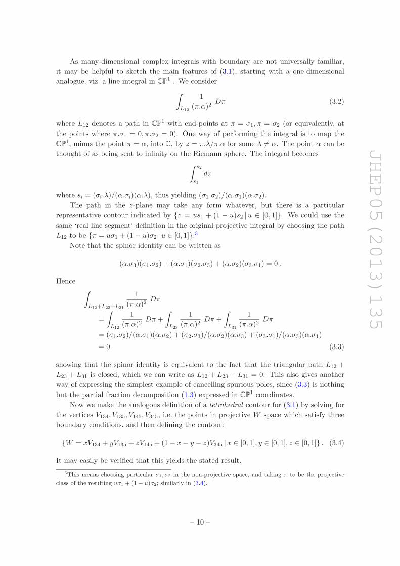
Figure 2. The polyhedron P6 = T13[46]5, with 6 vertices, 9 edges and 5 faces.

As in the one-dimensional analogue, this is only a representative contour. But the

properties of holomorphic functions ensure that the result of the integral is independent of

the representative. Although the ambient space is 6-real-dimensional, it is not misleading

to consider the integral as related to the volume of a tetrahedron. Because the incidence

properties of planes, lines and points in complex projective space are just the same as in

real spaces, it is also legitimate to picture the contour integrals using figures in three real

dimensions, and we shall do so in the following.

We now note that likewise

〈1365〉3

〈1235〉〈2365〉〈1236〉〈1265〉=

∫

T1365

6

(W.Z2)4DW , (3.5)

where T1365 has bounding faces W.Z1 = 0,W.Z3 = 0,W.Z5 = 0,W.Z6 = 0.

In both integrals, the necessary condition 〈1235〉 6= 0 can be interpreted as the

condition that the vertex V135 is a finite point when the bounding face corresponding to

Zα2 is sent to infinity.

3.1 Why spurious poles cancel: spurious boundaries

We have neglected questions of sign in the preceding discussion, (and the overall sign will

continue to neglected) but more precisely, we have tetrahedral contours equipped with an

orientation. We shall use the sign of the permutation to indicate relative orientation, thus

writing T1365 = −T1356. Then the difference between (3.1) and (3.5) is equivalent to inte-

grating over T1345 − T1365 = T1345 + T1356. This is a new polyhedron P6 = T13[46]5 with 6

vertices, 9 edges and 5 faces (see figure 2). The vertex V135 is absent. It follows that the

combined integral, giving the amplitude, remains finite even when the vertex V135 is at in-

finity. This explains geometrically why the pole 〈1235〉 no longer appears in the amplitude.

Our guiding idea is that spurious poles arise from spurious boundaries. If we consider

the amplitude to be given by the integration of (W.Z2)−4 over P6, which has no boundary

at the vertex (1235), the spurious pole never arises. The spurious poles only arise from

the representation of P6 as the difference of T1345 and T1365, which requires the insertion

of a spurious boundary.

– 11 –

JHEP05(2013)135

4

3

5

1

6

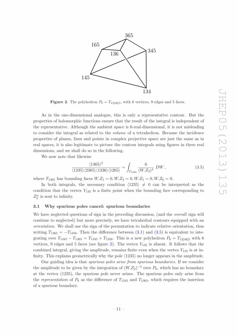
Figure 3. In the dual representation, P6 appears as the join of two tetrahedra, with 5 vertices, 9

edges and 6 faces.

An observation as elementary as school geometry now allows a marvellous application

of this identification of spurious boundaries. Note that P6 can be decomposed in a quite

different way into the sum of three tetrahedra:

P6 = T1346 + T3546 + T5146

This is most easily seen in the dual picture (figure 3), where these three tetrahedra meet

on their common edge {46}.

It follows that the volume of this polytope can also be written as

1

〈1246〉〈2346〉

(

〈1346〉3

〈1234〉〈1236〉

)

+1

〈2346〉〈2546〉

(

〈3546〉3

〈2345〉〈2356〉

)

+1

〈1246〉〈2546〉

(

〈5146〉3

〈1245〉〈1256〉

)

(3.6)

But this expression corresponds exactly to the formula (1.2) for the amplitude. Thus

twistor geometry reduces the hexagon identity almost to triviality in the special case of

split-helicity.

In this case it is the vertices V146, V346, V546 that correspond to spurious poles. (Again,

this is more easily seen in the dual picture, as in figure 3, where these vertices correspond

to the internal faces which split the polyhedron into three parts.)

The splitting of the polyhedron in two different ways can be stated in a more advanced

and elegant geometrical form. The five-term identity stating the equivalence of (1.1)

and (1.2) corresponds to the fact that the five tetrahedral hyperfaces of a 4-dimensional

simplex form a closed boundary. It is a higher-dimensional analogue of the closed triangle

in one dimension, L12 + L23 + L31 = 0. Algebraically, the spinor identity is equivalent to

T[aǫbc] = 0 for any T in two dimensions, and the five-term identity to T[aǫbcde] = 0 for any

T in four dimensions.

It is natural to refer to ‘spurious’ and ‘physical’ vertices, and we shall do so in what

follows. The definition of a physical vertex is that it is given by a quadruple which can

be put in the form (j, j + 1, k, k + 1) for some (j, k), and so corresponds to some physical

– 12 –

JHEP05(2013)135

+

5+

6+ 1

−2−

3−

4+ 1

−

2−

3−

4+5

+6+

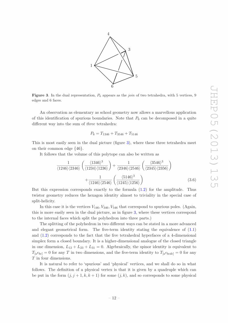
Figure 4. Twistor diagrams for the two-term representation of the split-helicity amplitude

A(1−2−3−4+5+6+).

pole. All the others are spurious. We have shown that P6 has only physical vertices, but

we want to ensure that this is not some special effect which applies to n = 6 alone.

3.2 Generalisation to more than six fields

In fact this geometric description readily generalizes to split-helicity n-field amplitudes in

the NMHV sector.

As preparation for doing this, and to complete the picture, we should first go back

to the case of NMHV for five fields in the split-helicity case. It is easy to verify that

A(1−2−3−4+5+) corresponds to integrating over the polyhedron P5 = T1345. That is,

A(1−2−3−4+5+) =[45]4

[12][23][34][45][51]=

〈12〉4〈23〉4

〈12〉〈23〉〈34〉〈45〉〈51〉

∫

P5

(W.Z2)−4DW .

Note that the change in going from five to six fields is very simple: (A) the denominator fac-

tor expands from five to six terms and (B) the new polyhedron is the sum of the polyhedron

for A(1−2−3−4+5+) and the polyhedron for A(1−2−3−5+6+). The same simple jump will

occur in going up to 7 and more fields, and it is worth exploiting its simplicity to avoid writ-

ing down long expressions analogous to (1.1) and (1.2). One way of doing this is through the

twistor diagram representation of the amplitudes. Nothing in what follows depends on using

the twistor diagram representation, but it is helpful in showing graphically the combinato-

rial aspects of the amplitudes. Furthermore, the feature of twistor diagrams that we shall

use now is one that Arkani-Hamed et al. [4] have pointed out as being of special interest.

The two-term formula (1.1) may be represented by the diagrams in figure 4. Here

we are using the definition of diagrams as given in [5]. The wavy lines are boundaries

and the quadruple lines are quadruple poles. In the super-symmetric extension developed

in [3, 7], these become super-components of diagrams in which all the edges represent

super-boundaries. However, the restriction to split-helicity makes it appropriate to revert

to the more elementary form. (The same features will be found in the diagrams defined

for the analogous split-signature amplitudes by Arkani-Hamed et al. [4], although their

wavy lines have a different meaning!)

– 13 –

JHEP05(2013)135

Note that the first of these diagrams can be seen as the result of using boundary-lines

to attach the 6-field to the twistor diagram for A(1−2−3−4+5+) and the second as the

result of attaching the 4-field to A(1−2−3−5+6+) similarly. This is no coincidence, and

it illustrates a general simplifying rule. This attachment can be seen as a special case of

the BCFW joining process, namely that which arises when one of the sub-amplitudes is

a 3-amplitude. There are two cases of this: joining an extra field to two twistor vertices

(black), or to two dual twistor vertices (white). Arkani-Hamed et al. [4] call this adding a

black or white triangle respectively, and give an interpretation of the attachment process

as the inverse of a soft limit. We may verify that when it is a black triangle that is added,

the effect on the amplitude is extremely simple in the new coordinates: the denominator

factors are expanded appropriately, and the polyhedron of integration remains unchanged.

This may seem surprising, because the ‘momentum shift’ seems to have been neglected.

The explanation is that it has gone into the re-definition of the momentum-twistors in

the new context. The polyhedron remains the same, but its interpretation in terms of the

external momenta changes in exactly the right way.

That P6 = T1345+T1356 follows immediately from this observation. This method takes

advantage of the fact, emphasised by Arkani-Hamed, that twistor diagrams make manifest

the many different ways in which a term can arise by the composition of sub-amplitudes.

The twistor diagrams for the 3-term expansion (1.2) can also be related to the

5-field amplitude, but not quite so simply: it needs the supersymmetric extension of the

‘attachment’ principle.

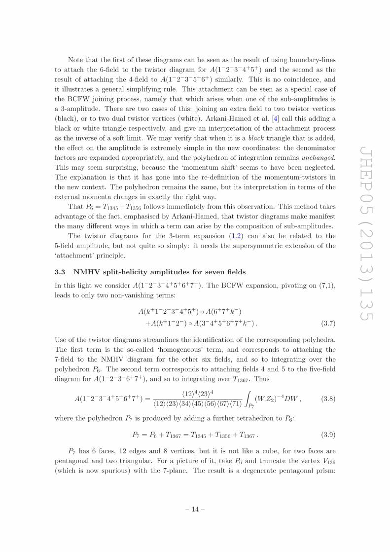
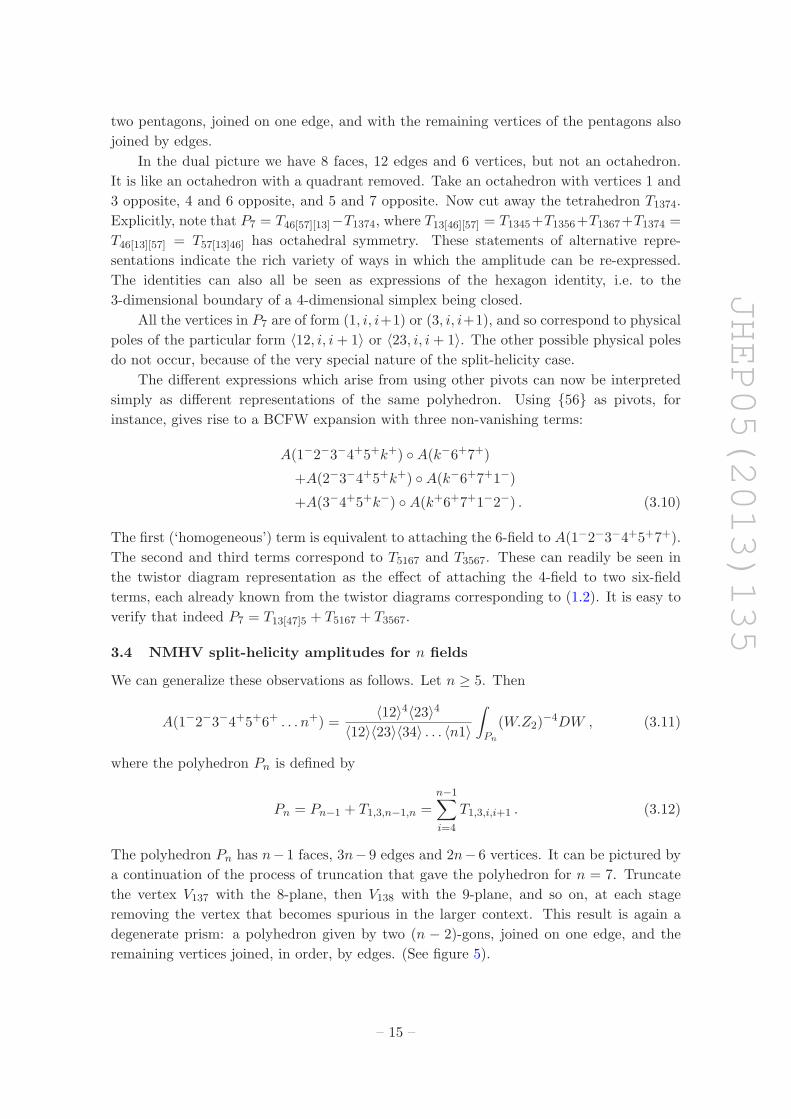
3.3 NMHV split-helicity amplitudes for seven fields

In this light we consider A(1−2−3−4+5+6+7+). The BCFW expansion, pivoting on (7,1),

leads to only two non-vanishing terms:

A(k+1−2−3−4+5+) ◦A(6+7+k−)

+A(k+1−2−) ◦A(3−4+5+6+7+k−) . (3.7)

Use of the twistor diagrams streamlines the identification of the corresponding polyhedra.

The first term is the so-called ‘homogeneous’ term, and corresponds to attaching the

7-field to the NMHV diagram for the other six fields, and so to integrating over the

polyhedron P6. The second term corresponds to attaching fields 4 and 5 to the five-field

diagram for A(1−2−3−6+7+), and so to integrating over T1367. Thus

A(1−2−3−4+5+6+7+) =〈12〉4〈23〉4

〈12〉〈23〉〈34〉〈45〉〈56〉〈67〉〈71〉

∫

P7

(W.Z2)−4DW , (3.8)

where the polyhedron P7 is produced by adding a further tetrahedron to P6:

P7 = P6 + T1367 = T1345 + T1356 + T1367 . (3.9)

P7 has 6 faces, 12 edges and 8 vertices, but it is not like a cube, for two faces are

pentagonal and two triangular. For a picture of it, take P6 and truncate the vertex V136(which is now spurious) with the 7-plane. The result is a degenerate pentagonal prism:

– 14 –

JHEP05(2013)135

two pentagons, joined on one edge, and with the remaining vertices of the pentagons also

joined by edges.

In the dual picture we have 8 faces, 12 edges and 6 vertices, but not an octahedron.

It is like an octahedron with a quadrant removed. Take an octahedron with vertices 1 and

3 opposite, 4 and 6 opposite, and 5 and 7 opposite. Now cut away the tetrahedron T1374.

Explicitly, note that P7 = T46[57][13]−T1374, where T13[46][57] = T1345+T1356+T1367+T1374 =

T46[13][57] = T57[13]46] has octahedral symmetry. These statements of alternative repre-

sentations indicate the rich variety of ways in which the amplitude can be re-expressed.

The identities can also all be seen as expressions of the hexagon identity, i.e. to the

3-dimensional boundary of a 4-dimensional simplex being closed.

All the vertices in P7 are of form (1, i, i+1) or (3, i, i+1), and so correspond to physical

poles of the particular form 〈12, i, i+ 1〉 or 〈23, i, i+ 1〉. The other possible physical poles

do not occur, because of the very special nature of the split-helicity case.

The different expressions which arise from using other pivots can now be interpreted

simply as different representations of the same polyhedron. Using {56} as pivots, for

instance, gives rise to a BCFW expansion with three non-vanishing terms:

A(1−2−3−4+5+k+) ◦A(k−6+7+)

+A(2−3−4+5+k+) ◦A(k−6+7+1−)

+A(3−4+5+k−) ◦A(k+6+7+1−2−) . (3.10)

The first (‘homogeneous’) term is equivalent to attaching the 6-field to A(1−2−3−4+5+7+).

The second and third terms correspond to T5167 and T3567. These can readily be seen in

the twistor diagram representation as the effect of attaching the 4-field to two six-field

terms, each already known from the twistor diagrams corresponding to (1.2). It is easy to

verify that indeed P7 = T13[47]5 + T5167 + T3567.

3.4 NMHV split-helicity amplitudes for n fields

We can generalize these observations as follows. Let n ≥ 5. Then

A(1−2−3−4+5+6+ . . . n+) =〈12〉4〈23〉4

〈12〉〈23〉〈34〉 . . . 〈n1〉

∫

Pn

(W.Z2)−4DW , (3.11)

where the polyhedron Pn is defined by

Pn = Pn−1 + T1,3,n−1,n =n−1∑

i=4

T1,3,i,i+1 . (3.12)

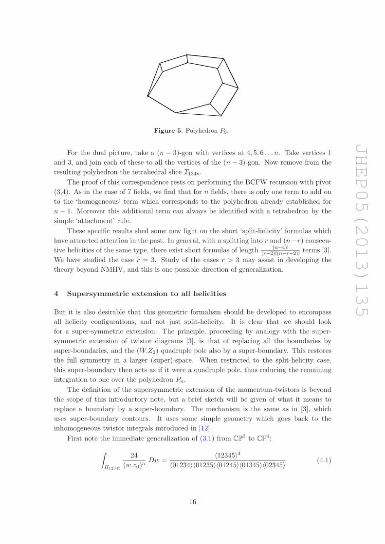
The polyhedron Pn has n− 1 faces, 3n− 9 edges and 2n− 6 vertices. It can be pictured by

a continuation of the process of truncation that gave the polyhedron for n = 7. Truncate

the vertex V137 with the 8-plane, then V138 with the 9-plane, and so on, at each stage

removing the vertex that becomes spurious in the larger context. This result is again a

degenerate prism: a polyhedron given by two (n − 2)-gons, joined on one edge, and the

remaining vertices joined, in order, by edges. (See figure 5).

– 15 –

JHEP05(2013)135

Figure 5. Polyhedron P9.

For the dual picture, take a (n − 3)-gon with vertices at 4, 5, 6 . . . n. Take vertices 1

and 3, and join each of these to all the vertices of the (n − 3)-gon. Now remove from the

resulting polyhedron the tetrahedral slice T134n.

The proof of this correspondence rests on performing the BCFW recursion with pivot

(3,4). As in the case of 7 fields, we find that for n fields, there is only one term to add on

to the ‘homogeneous’ term which corresponds to the polyhedron already established for

n − 1. Moreover this additional term can always be identified with a tetrahedron by the

simple ‘attachment’ rule.

These specific results shed some new light on the short ‘split-helicity’ formulas which

have attracted attention in the past. In general, with a splitting into r and (n−r) consecu-

tive helicities of the same type, there exist short formulas of length (n−4)!(r−2)!(n−r−2)! terms [3].

We have studied the case r = 3. Study of the cases r > 3 may assist in developing the

theory beyond NMHV, and this is one possible direction of generalization.

4 Supersymmetric extension to all helicities

But it is also desirable that this geometric formalism should be developed to encompass

all helicity configurations, and not just split-helicity. It is clear that we should look

for a super-symmetric extension. The principle, proceeding by analogy with the super-

symmetric extension of twistor diagrams [3], is that of replacing all the boundaries by

super-boundaries, and the (W.Z2) quadruple pole also by a super-boundary. This restores

the full symmetry in a larger (super)-space. When restricted to the split-helicity case,

this super-boundary then acts as if it were a quadruple pole, thus reducing the remaining

integration to one over the polyhedron Pn.

The definition of the supersymmetric extension of the momentum-twistors is beyond

the scope of this introductory note, but a brief sketch will be given of what it means to

replace a boundary by a super-boundary. The mechanism is the same as in [3], which

uses super-boundary contours. It uses some simple geometry which goes back to the

inhomogeneous twistor integrals introduced in [12].

First note the immediate generalization of (3.1) from CP3 to CP

4:

∫

H12345

24

(w.z0)5Dw =

〈12345〉4

〈01234〉〈01235〉〈01245〉〈01345〉〈02345〉(4.1)

– 16 –

JHEP05(2013)135

where w, zi are CP4 variables, Dw the natural projective 4-form, H12345 is the simplex with

five hyperfaces on w.z1 = 0, . . . w.z5 = 0, and 〈12345〉 stands for ǫαβγδθzα1 z

β2 z

γ3 z

δ4z

θ5 .

If CP4, minus the hyperplane {w|(w.z0) = 0}, is mapped onto dual twistor space

T∗ ≃ C

4, the CP4 integral (4.1) becomes:

24

∫

H

D4W

where H is a 4-dimensional contour with boundaries on the hyperfaces of a simplex, which

may be given in the form

W.Z1 + c1 = 0, W.Z2 + c2 = 0, W.Z3 + c3 = 0, W.Z4 + c4 = 0, W.Z5 + c5 = 0 .

The result, which can now be interpreted as (24 times the) complex 4-volume of this

simplex, is∣

∣

∣

∣

∣

∣

∣

∣

∣

∣

∣

c1 Z01 Z

11 Z

21 Z

31

c2 Z02 Z

12 Z

22 Z

32

c3 Z03 Z

13 Z

23 Z

33

c4 Z04 Z

14 Z

24 Z

34

c5 Z05 Z

15 Z

25 Z

35

∣

∣

∣

∣

∣

∣

∣

∣

∣

∣

∣

4

〈1234〉〈1235〉〈1245〉〈1345〉〈2345〉. (4.2)

This calculation could be done directly in C4 without reference to CP

4, for this formula

is simply the complexification of some elementary Euclidean geometry. But the projective

description may be helpful by suggesting an analogy with the 3-dimensional tetrahedral

contour described in (3.1) where a plane in projective twistor space is sent to infinity in

C3 coordinates.

The formula (4.2) is simply a rational function of all the variables, and in particular

a quartic polynomial in the ci. If we have linear relationships between the 4-volumes of

such simplexes (such as will be discussed in the next section), then they define identities

between the corresponding rational functions. Multiplying up by the denominators, they

are simply identities between polynomials.

Super-boundaries are formally defined as boundaries on W.Zi + φ.ψi = 0, where φ

is the anticommuting part of the dual supertwistor W , and ψi is the anticommuting

part of the supertwistor Zi. The result of the integration over a simplex in super-space,

with hyperfaces given by five such super-boundaries, can thus be unambiguously defined

by replacing the ci in (4.2) by (φ.ψi). Polynomial identities will be preserved in this

replacement, so that linear relationships between 4-polytopes will imply the analogous

relationships between super-volumes in super-space.

After making this replacement in (4.2), the formal integration over φ1, φ2, φ3, φ4 is

immediate and leads to

(∑5

i=1 ψi〈i+ 1, i+ 2, i+ 3, i+ 4〉)4

〈1234〉〈1235〉〈1245〉〈1345〉〈2345〉, (4.3)

as (24 times) the super-volume of the super-simplex. This gives the geometric basis for

the supersymmetric theory. Informally, the construction is like treating the ‘fermionic’

– 17 –

JHEP05(2013)135

part of a supertwistor as a single extra dimension, choosing coordinates in which ‘clas-

sical’ twistors, those with no fermionic part, are sent to infinity, and then measuring a

super-volume in the resulting space.

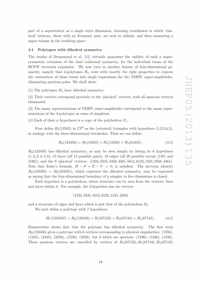
4.1 Polytopes with dihedral symmetry

The results of Drummond et al. [11] virtually guarantee the validity of such a super-

symmetric extension of the dual conformal symmetry, for the individual terms of the

BCFW recursion expansion. We now turn to another feature of four-dimensional ge-

ometry, namely that 4-polytopes Hn exist with exactly the right properties to express

the summation of those terms into single expressions for the NMHV super-amplitudes,

eliminating spurious poles. We shall show:

(1) The polytopes Hn have dihedral symmetry.

(2) Their vertices correspond precisely to the ‘physical’ vertices, with all spurious vertices

eliminated.

(3) The many representations of NMHV super-amplitudes correspond to the many repre-

sentations of the 4-polytopes as sums of simplexes.

(4) Each of their n hyperfaces is a copy of the polyhedron Pn.

First define H5(12345) in CP4 as the (oriented) 5-simplex with hyperfaces (1,2,3,4,5),

in analogy with the three-dimensional tetrahedra. Then we can define:

H6(123456) = H5(12345) +H5(12356) +H5(61345) . (4.4)

H6(123456) has dihedral symmetry, as may be seen simply by listing its 6 hyperfaces

(1, 2, 3, 4, 5, 6), 15 faces (all 15 possible pairs), 18 edges (all 20 possible except (135) and

(246)), and the 9 ‘physical’ vertices: (1234, 2345, 3456, 4561, 5612, 6123, 1245, 2356, 3461).

Note that Euler’s formula, H − F + E − V = 0, is satisfied. The six-term identity

H6(123456) = H6(234561), which expresses the dihedral symmetry, may be expressed

as saying that the four-dimensional boundary of a simplex in five dimensions is closed.

Each hyperface is a polyhedron, whose structure can be seen from the vertices, lines

and faces within it. For example, the 2-hyperface has six vertices

(1234, 2345, 5612, 6123, 1245, 2356)

and a structure of edges and faces which is just that of the polyhedron P6.

We next define a polytope with 7 hyperfaces:

H7(1234567) = H6(123456) +H5(67123) +H5(67134) +H5(67145) . (4.5)

Enumeration shows that that the polytope has dihedral symmetry. The first term

H6(123456) gives a polytope with 6 vertices corresponding to physical singularities: (1234),

(1245), (2345), (3456), (1256), (2356), but 3 which are spurious: (1236), (1346), (1456).

These spurious vertices are cancelled by vertices of H5(67123), H5(67134), H5(67145)

– 18 –

JHEP05(2013)135

respectively. Likewise one may verify that H5(67123), H5(67134), H5(67145) supply the

further 8 ‘physical’ vertices, whilst 2 further spurious vertices (6714), (6713) cancel

between themselves. The resulting polytope has 14 vertices, 28 edges, 21 faces and 7

hyperfaces, and despite the asymmetry of its definition, has complete dihedral symmetry.

Each hyperface is like the ‘degenerate prism’ polyhedron P7.

It is straightforward to give an inductive rule for the sum of 12(n−4)(n−3) simplexes,

which generalizes the case of n = 7:

Hn(123 . . . n) = Hn−1(123 . . . n− 1) +n−4∑

j=1

H5(n− 1, n, 1, j + 1, j + 2) . (4.6)

The leading term generates (n− 4) spurious vertices, namely

(n− 3, n− 2, n− 1, 1), (n− 4, n− 3, n− 1, 1), . . . (3, 4, n− 1, 1), (2, 3, n− 1, 1).

The jth of these is cancelled by a spurious vertex from the jth of the tail terms.

The j = 1 tail term has one further spurious vertex, namely (n− 1, n, 1, n− 3), which

cancels with the same vertex arising in the j = 2 term. The j = n − 4 term also has just

one further spurious vertex, (n− 1, n, 1, 3), which cancels with the vertex in the j = n− 5

term. Otherwise, for each j = 3, 4, 5 . . . n − 5, the jth term have three spurious vertices,

one cancelling with the leading term, and the others cancelling with vertices from the

(j − 1)th and (j + 1)th terms.

The polytope Hn has 12n(n−3) vertices (corresponding to the physical poles), n(n−3)

edges, 12n(n − 1) faces and n hyperfaces. Each hyperface is a polyhedron Pn, as may

readily verified from the recursive definition of Hn. At each stage, its intersection with

the 2-hyperface agrees with the recursive definition of Pn.

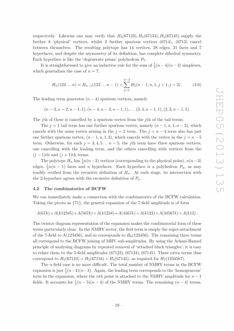
4.2 The combinatorics of BCFW

We can immediately make a connection with the combinatorics of the BCFW calculation.

Taking the pivots as {71}, the general expansion of the 7-field amplitude is of form

A(67k) ◦A(k12345)+A(567k) ◦A(k1234)+A(4567k) ◦A(k123)+A(34567k) ◦A(k12) .

The twistor diagram representation of the expansion makes the combinatorial form of these

terms particularly clear. In the NMHV sector, the first term is simply the super-attachment

of the 7-field to A(123456), and so corresponds to H6(123456). The remaining three terms

all correspond to the BCFW joining of MHV sub-amplitudes. By using the Arkani-Hamed

principle of analysing diagrams by repeated removal of ‘attached black triangles’, it is easy

to relate them to the 5-field amplitudes (67123), (67134), (67145). These extra terms thus

correspond to H5(67123) +H5(67134) +H5(67145), as required for H7(1234567).

The n-field case is no more difficult. The total number of NMHV terms in the BCFW

expansion is just 12(n−4)(n−3). Again, the leading term corresponds to the ‘homogeneous’

term in the expansion, where the nth point is attached to the NMHV amplitude for n− 1

fields. It accounts for 12(n− 5)(n− 4) of the NMHV terms. The remaining (n− 4) terms,

– 19 –

JHEP05(2013)135

by using the supersymmetric attachment rule, are easily seen to correspond one by one

to the remaining simplexes in the definition of the Hn. Different choices of pivots simply

correspond to different representations of the Hn, and all of these representations are

related by the ‘hexagon identity’ which now has a fundamental geometrical meaning.

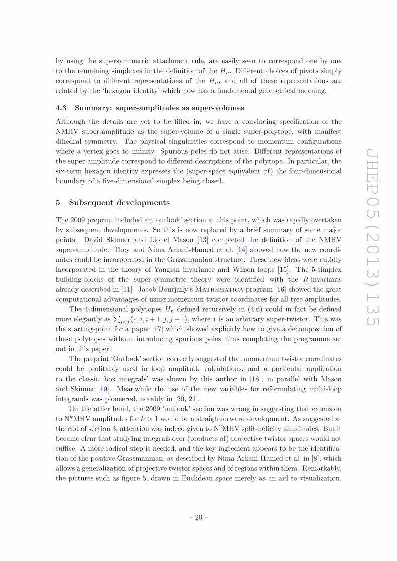
4.3 Summary: super-amplitudes as super-volumes

Although the details are yet to be filled in, we have a convincing specification of the

NMHV super-amplitude as the super-volume of a single super-polytope, with manifest

dihedral symmetry. The physical singularities correspond to momentum configurations

where a vertex goes to infinity. Spurious poles do not arise. Different representations of

the super-amplitude correspond to different descriptions of the polytope. In particular, the

six-term hexagon identity expresses the (super-space equivalent of) the four-dimensional

boundary of a five-dimensional simplex being closed.

5 Subsequent developments

The 2009 preprint included an ‘outlook’ section at this point, which was rapidly overtaken

by subsequent developments. So this is now replaced by a brief summary of some major

points. David Skinner and Lionel Mason [13] completed the definition of the NMHV

super-amplitude. They and Nima Arkani-Hamed et al. [14] showed how the new coordi-

nates could be incorporated in the Grassmannian structure. These new ideas were rapidly

incorporated in the theory of Yangian invariance and Wilson loops [15]. The 5-simplex

building-blocks of the super-symmetric theory were identified with the R-invariants

already described in [11]. Jacob Bourjaily’s Mathematica program [16] showed the great

computational advantages of using momentum-twistor coordinates for all tree amplitudes.

The 4-dimensional polytopes Hn defined recursively in (4.6) could in fact be defined

more elegantly as∑

i<j〈∗, i, i+1, j, j +1〉, where ∗ is an arbitrary super-twistor. This was

the starting-point for a paper [17] which showed explicitly how to give a decomposition of

these polytopes without introducing spurious poles, thus completing the programme set

out in this paper.

The preprint ‘Outlook’ section correctly suggested that momentum twistor coordinates

could be profitably used in loop amplitude calculations, and a particular application

to the classic ‘box integrals’ was shown by this author in [18], in parallel with Mason

and Skinner [19]. Meanwhile the use of the new variables for reformulating multi-loop

integrands was pioneered, notably in [20, 21].

On the other hand, the 2009 ‘outlook’ section was wrong in suggesting that extension

to NkMHV amplitudes for k > 1 would be a straightforward development. As suggested at

the end of section 3, attention was indeed given to N2MHV split-helicity amplitudes. But it

became clear that studying integrals over (products of) projective twistor spaces would not

suffice. A more radical step is needed, and the key ingredient appears to be the identifica-

tion of the positive Grassmannian, as described by Nima Arkani-Hamed et al. in [8], which

allows a generalization of projective twistor spaces and of regions within them. Remarkably,

the pictures such as figure 5, drawn in Euclidean space merely as an aid to visualization,

– 20 –

JHEP05(2013)135

turn out to be prototypes of the vital ‘positivity’ property. The correct generalization of

super-volume, however, has not yet been elucidated. These developments have been ad-

vanced by collaborations with leading geometers, to whom the polytopes identified in this

paper as Hn are familiar as cyclic polytopes, and the subject of great contemporary interest.

Dual conformal invariance depends on a given colour-ordering, and it is not clear

whether momentum-twistor coordinates can usefully be employed to express relations

between amplitudes of different colour-orderings. The same question applies to non-planar

loop amplitudes and to gravitational amplitudes. Nevertheless, momentum twistors may

usefully encode momentum conservation even when no colour ordering is preferred. This

idea has been applied to re-express gravitational MHV amplitudes [22], and has led to a

useful new result [23].

Acknowledgments

This work was encouraged and stimulated by participation in a workshop at the Perimeter

Institute in December 2008 organised by Freddy Cachazo and Nima Arkani-Hamed,

and the writer is grateful to the Perimeter Institute for its generous invitation. The

expositions of the distinguished participants in the International Workshop on Gauge

and String Amplitudes at Durham University, March/April 2009, especially that of Nima

Arkani-Hamed, also helped to focus the questions addressed in this note. I am also

grateful to my colleagues David Skinner and Lionel Mason, especially for discussion of the

super-symmetric extension of the integrals.

References

[1] R. Britto, F. Cachazo, B. Feng and E. Witten, Direct proof of tree-level recursion relation in

Yang-Mills theory, Phys. Rev. Lett. 94 (2005) 181602 [hep-th/0501052] [INSPIRE].

[2] N. Arkani-Hamed, F. Cachazo and J. Kaplan, What is the simplest quantum field theory?,

JHEP 09 (2010) 016 [arXiv:0808.1446] [INSPIRE].

[3] A.P. Hodges, Twistor diagrams for all tree amplitudes in gauge theory: a

Helicity-independent formalism, hep-th/0512336 [INSPIRE].

[4] N. Arkani-Hamed, F. Cachazo, C. Cheung and J. Kaplan, The S-matrix in twistor space,

JHEP 03 (2010) 110 [arXiv:0903.2110] [INSPIRE].

[5] A.P. Hodges, Twistor diagram recursion for all gauge-theoretic tree amplitudes,

hep-th/0503060 [INSPIRE].

[6] L. Mason and D. Skinner, Scattering amplitudes and BCFW recursion in twistor space,

JHEP 01 (2010) 064 [arXiv:0903.2083] [INSPIRE].

[7] A.P. Hodges, Scattering amplitudes for eight gauge fields, hep-th/0603101 [INSPIRE].

[8] N. Arkani-Hamed et al., Scattering amplitudes and the positive Grassmannian,

arXiv:1212.5605 [INSPIRE].

[9] A. Brandhuber, P. Heslop and G. Travaglini, A note on dual superconformal symmetry of the

N = 4 super Yang-Mills S-matrix, Phys. Rev. D 78 (2008) 125005 [arXiv:0807.4097]

[INSPIRE].

– 21 –

JHEP05(2013)135

[10] J. Drummond, J. Henn, V. Smirnov and E. Sokatchev, Magic identities for conformal

four-point integrals, JHEP 01 (2007) 064 [hep-th/0607160] [INSPIRE].

[11] J. Drummond, J. Henn, G. Korchemsky and E. Sokatchev, Dual superconformal symmetry of

scattering amplitudes in N = 4 super-Yang-Mills theory, Nucl. Phys. B 828 (2010) 317

[arXiv:0807.1095] [INSPIRE].

[12] A.P. Hodges, A twistor approach to the regularization of divergences,

Proc. Roy. Soc. Lond. A 397 (1985) 341 [INSPIRE].

[13] L. Mason and D. Skinner, Dual superconformal invariance, momentum twistors and

Grassmannians, JHEP 11 (2009) 045 [arXiv:0909.0250] [INSPIRE].

[14] N. Arkani-Hamed, F. Cachazo and C. Cheung, The Grassmannian origin of dual

superconformal invariance, JHEP 03 (2010) 036 [arXiv:0909.0483] [INSPIRE].

[15] J. Drummond and L. Ferro, Yangians, Grassmannians and T-duality, JHEP 07 (2010) 027

[arXiv:1001.3348] [INSPIRE].

[16] J.L. Bourjaily, Efficient tree-amplitudes in N = 4: automatic BCFW recursion in

Mathematica, arXiv:1011.2447 [INSPIRE].

[17] N. Arkani-Hamed, J.L. Bourjaily, F. Cachazo, A. Hodges and J. Trnka, A note on polytopes

for scattering amplitudes, JHEP 04 (2012) 081 [arXiv:1012.6030] [INSPIRE].

[18] A. Hodges, The box integrals in momentum-twistor geometry, arXiv:1004.3323 [INSPIRE].

[19] L. Mason and D. Skinner, Amplitudes at weak coupling as polytopes in AdS5,

J. Phys. A 44 (2011) 135401 [arXiv:1004.3498] [INSPIRE].

[20] N. Arkani-Hamed, J.L. Bourjaily, F. Cachazo, S. Caron-Huot and J. Trnka, The all-loop

integrand for scattering amplitudes in planar N = 4 SYM, JHEP 01 (2011) 041

[arXiv:1008.2958] [INSPIRE].

[21] N. Arkani-Hamed, J.L. Bourjaily, F. Cachazo and J. Trnka, Local integrals for planar

scattering amplitudes, JHEP 06 (2012) 125 [arXiv:1012.6032] [INSPIRE].

[22] A. Hodges, New expressions for gravitational scattering amplitudes, arXiv:1108.2227

[INSPIRE].

[23] A. Hodges, A simple formula for gravitational MHV amplitudes, arXiv:1204.1930 [INSPIRE].

– 22 –