Institut d’Economie Industrielle (IDEI) – Manufacture des TabacsAile Jean-Jacques Laffont – 21, allée de Brienne – 31000 TOULOUSE – FRANCETél. + 33(0)5 61 12 85 89 – Fax + 33(0)5 61 12 86 37 – www.idei.fr – contact@cict.fr

April, 2010

n° 643

“Eliciting Beliefs: Proper Scoring Rules, Incentives, Stakes and

Hedging”

Olivier ARMANTIER and Nicolas TREICH

Eliciting Beliefs: Proper Scoring Rules,

Incentives, Stakes and Hedging�

Olivier Armantiery Nicolas Treichz

April 15, 2010

Abstract

Accurate measurements of probabilistic beliefs have become increasingly im-portant both in practice and in academia. Introduced by statisticians in the1950s to promote truthful reports in simple environments, Proper Scoring Rules(PSR) are now arguably the most popular incentivized mechanisms to elicit anagent�s beliefs. This paper generalizes the analysis of PSR to richer environmentsrelevant to economists. More speci�cally, we combine theory and experiment tostudy how beliefs reported with a PSR may be biased when i) the PSR paymentsare increased, ii) the agent has a �nancial stake in the event she is predicting, andiii) the agent can hedge her prediction by taking an additional action. Our resultsreveal complex distortions of reported beliefs, thereby raising concerns about theability of PSR to recover truthful beliefs in general economic environments.

�We would especially like to thank Amadou Boly and Alexander Wagner for their help and insights duringthe course of this research project. We also thank Alexander Koch, Peter Wakker, and Bob Winkler as wellas seminar participants at the Universities of Bergen and Christchurch and at the ESA conferences in Tucsonand Melbourne for helpful discussions. All remaining errors are ours. The views expressed in this paper arethose of the authors and do not necessarily represent the views of the Federal Reserve Bank of New Yorkor the Federal Reserve System. Nicolas Treich acknowledges the chair �Marché des risques et création devaleurs�, Fondation du risque/SCOR, for �nancial support.

yFederal Reserve Bank of New York, U.S. E-mail: olast1@gmail.com.zToulouse School of Economics (LERNA, INRA), France. E-mail: ntreich@toulouse.inra.fr

1. Introduction

Introduced by statisticians in the 1950s, Proper Scoring Rules (PSR hereafter) are belief

elicitation techniques designed to provide an agent the incentives to report her subjective

beliefs in a thoughtful and truthful manner.1 Although the analysis of PSR has recently

been generalized to modern theories of risk and ambiguity (O¤erman et al. 2009), the

properties of PSR have yet to be characterized in general economic environments. This

paper combines theory and experiment in an attempt at partially �lling this void. More

precisely, we characterize the possible PSR biases (i.e. the systematic di¤erences between

an agent�s subjective and reported beliefs) for all risk averse agents and all PSR under three

e¤ects: i) a change in the PSR payments, ii) the introduction of a �nancial stake in the

event the agent is predicting, and iii) the possibility for the agent to hedge her prediction

by taking an additional action. The empirical signi�cance of the biases identi�ed are then

tested in an experiment.

Accurate measurements of probabilistic beliefs have become increasingly important both

in practice and in academia. In practice, numerous websites now o¤er public opinions (about

e.g. consumer products, movies, or restaurants) and predictions (about e.g. sporting or

political events).2 To be meaningful, these opinions and predictions must be informative.

When soliciting advice from experts (about e.g. health, environmental, or �nancial issues)

individuals typically expect unbiased recommendations. Recent suspicions of con�ict of

1Early references in statistics include Brier (1950), Good (1952) and McCarthy (1956). Interestingly, itseems that De Finetti �rst introduced PSR (De Finetti 1981). A broad and in�uential paper in the statisticalliterature is Savage (1971). Early references in economics include Friedman (1979) and Holt (1979).

2Such opinion websites include ePinion, Ebay, Zagat, or Amazon. Prediction websites include the IowaElectronic Market, the Hollywood Stock Exchange, or Intrade.

2

interest suggest that this may not always be the case.3 Finally, in an e¤ort to better manage

risk, �rms are increasingly turning to their employees to forecast (e.g.) sales, completion

dates, or industry trends.4 Precise belief assessments are also important in academia. In

particular, Manski (2002, 2004) argues that separate measures of choices and beliefs are

useful to estimate decision models properly. Modern macroeconomic theory considers that

monetary policy consists in large part in managing expectations (about e.g. in�ation),

which requires correct measures of probabilistic beliefs.5 Finally, experimental economists

are increasingly eliciting their subjects�beliefs to understand observed behavior better.6

Because they are incentive compatible under expected payo¤ maximization, PSR have

been one of the most popular belief elicitation techniques, with applications to numerous

�elds such as meteorology, business, education, psychology, �nance, and economics.7 Re-

cently, with the rapid development of prediction markets, there has been an upsurge of

interest in PSR. In particular, Market Scoring Rules have been proposed as a way to over-

come the liquidity problems that have a¤ected some prediction markets.8 In short, Market

Scoring Rules may be described as follows. A group of agents is sequentially asked to make

a prediction about a particular event. Each agent is paid for her prediction according to a

PSR, but she also agrees to pay the previous agent for his prediction according to the same

3See e.g. the New York Times article �Questions Grow About a Top CNBC Anchor�(February 12, 2007)about TV anchors for the �nancial news channel CNBC. Likewise, the pharmaceutical industry has longbeen suspected to in�uence doctors�prescription behavior through various �marketing�campaigns.

4Such �rms include Yahoo!, Microsoft, Google, Chevron, General Electric, and General Motors. Theeconomic value of accurate forecasts may be illustrated with the case of the Dreamliner�s delays which areexpected to cost the Boeing Corporation up to $10 billion.

5See e.g. Woodford (2005), or Blinder et al. (2008) for a review of this literature. Note also that e¤ortsare currently underway at the Federal Reserve Bank of New York to develop better instruments to measureindividuals�in�ation expectations (Bruine de Bruin et al. 2009).

6Wagner (2009) identi�es more than 40 economic experiments using incentivized beliefs elicitation tech-niques.

7See Camerer (1995), O¤erman et al. (2009), or Palfrey and Wang (2009) for references.8See, e.g., Hanson (2003), Ledyard (2006) or Abramowicz (2007).

3

PSR. Because of their attractive properties, Market Scoring Rules have been rapidly adopted

by several �rms operating prediction markets.9

It has long been recognized, however, that PSR can generate biases when agents are

not risk neutral (Winkler and Murphy 1970). The nature of these biases has typically been

analyzed in simple and speci�c contexts. Namely, a particular PSR and a given utility

function are selected, and the agent�s wealth is generally assumed to vary only with the PSR

payments. This paper contributes to the literature by extending the analysis i) to all PSR

and ii) to richer economic environments. More precisely, we characterize the possible biases

PSR generate in response to three e¤ects.

First, we consider how varying the PSR payments a¤ects reported probabilities. Al-

though experimental economists have long debated how incentives a¤ect choices (Camerer

and Hogarth 1999, Hertwig and Ortmann 2001), to the best of our knowledge, the problem

has not been explicitly addressed for PSR.10

Second, we consider an environment in which the agent has a �nancial stake in the event,

a situation common in practice. For instance, an agent may be asked to make a prediction

about an economic indicator (e.g. the stock market, the in�ation level) or an event (e.g. a

�ood, a favorable jury verdict). Similarly, an agent facing a Market Scoring Rule always has

a stake in the event she predicts, as her payment to the previous predictor depends on the

outcome of the event. Finally, subjects in (e.g.) public good experiments are often asked to

predict the contributions of others.11 In all those cases, independently of the PSR payments,

9E.g. Inkling Markets, Consensus Point, Yoopick, Crowdcast, and Microsoft Corporation.10Some have compared �nancially versus non-�nancially incentivized belief elicitation techniques (Beach

and Philips 1967, Rutström and Wilcox 2009). We extend this analysis by considering variations of strictlypositive �nancial incentives.11See e.g. Croson (2000), Gachter and Renner (2006), or Fischbacher and Gachter (2008).

4

the agent�s wealth varies with the outcome of the random variable she is predicting. As we

shall see, such violations of the �no stake�condition (Kadane and Winkler 1988) may induce

further biases.

Third, we o¤er the agent the possibility of hedging her prediction by taking an additional

action whose payo¤ also depends on the event. For instance, in the previous examples,

the agent predicting an economic indicator might also have to choose how to diversify her

portfolio, while the agent predicting a catastrophic event may also have to decide on her

insurance coverage. Likewise, subjects in public good experiments have to choose their own

contributions.12 As we shall see, because they are not independent, the prediction and

the additional action are in general di¤erent from what each decision would be if made

separately. In such cases, we show that hedging creates an additional source of bias in the

reported probabilities.

Our analysis is divided in three parts. In the theory part, we assume expected utility

and consider the class of all PSR for binary events (Gneiting and Raftery 2007). We �rst

show that there is a monotone relationship between reported and subjective probabilities.

We then generalize previous results (Winkler and Murphy 1970, O¤erman et al. 2009,

Andersen et al. 2009) by showing that risk averters report more uniform probabilities,

i.e. probabilities skewed toward 1/2. In contrast to popular belief, we �nd that changing

the rewards of the PSR has an ambiguous impact on reported probabilities. In particular,

smaller PSR payments can either reduce or reinforce the PSR biases depending on whether

12Although experimental economists have recently been aware of stakes and hedging opportunities (Fehret al. 2009, Palfrey and Wang 2009, Andersen et al. 2009), these issues have typically been ignored (Costa-Gomez and Weizsacker 2008, Fischbacher and Gachter 2008). Concerns have also been raised that elicitingbeliefs of subjects engaged in a game, even absent any stakes and hedging considerations, may lead them tothink more strategically, therefore a¤ecting their behavior (Croson 2000, Gachter and Renner 2006, Rutströmand Wilcox 2009).

5

the utility function displays increasing or decreasing relative risk aversion. We then show

that the presence of a bonus (i.e. a positive stake) when the event occurs, lowers reported

probabilities under risk aversion. Finally, we show that the possibility of hedging by betting

on the event can severely alter predictions. In particular, we identify a region in our model

where the reported probabilities remain unchanged and are therefore completely independent

of the agent�s subjective probabilities.

In the second part, we report on an experiment aimed at testing whether the biases

induced by PSR are empirically relevant. The basic design is similar to O¤erman et al.

(2009) (OSKW hereafter). Subjects are presented with a list of events describing the possible

outcome of the roll of two 10-sided dice. The probabilities are elicited with a quadratic scoring

rule. In addition to a control treatment, six treatments are conducted by varying i) the PSR

payments (the �High Incentives� and �Hypothetical Incentives� treatments), ii) the stake

in the event (the �Low Stakes�and �High Stakes�treatments), and iii) the returns on the

amount bet on the event (the �Low Hedging�and �High Hedging�treatments). Although

not perfectly consistent in magnitude, the experimental results are generally in line with

the directions of the theoretical predictions made under risk aversion. In particular, we �nd

signi�cantly larger biases when the PSR pays higher amounts, which suggests that subjects

exhibit increasing relative risk aversion. In contrast, the absence of incentives produces less

biased yet noisier elicited probabilities. Consistent with the theory, the presence of a stake

leads subjects to report signi�cantly lower probabilities. Furthermore, we �nd a positive

correlation between the amount bet on an event and the bias in the reported probability for

that event, thereby providing evidence of hedging. Finally, we observe larger biases when the

underlying objective probabilities are compounded or complex, which, although inconsistent

6

with expected utility, can be rationalized with a model of ambiguity aversion.

Finally, we discuss in the third part some implications of our results for the elicitation

of beliefs with PSR in general economic environments. We conclude that accurate measures

of subjective probabilities may be di¢ cult to obtain in the �eld. For lab experiments,

we discuss the e¤ectiveness of possible remedial measures that could be taken to recover

subjective probabilities when subjects have a stake or a hedging opportunity.

2. Theory

In this section, we study the properties of the �response function�, that is the function that

gives the optimal reported probabilities of an agent who is rewarded according to a PSR.

The properties derived hold for all PSR, and are therefore not restricted to the quadratic

scoring rule (QSR hereafter) we use in the experiment.

2.1. Preliminary Assumptions

We consider a binary random variable, that is, an event and its complement. We assume

probabilistic sophistication, and thus restrict our attention to the subjective probability of

this event p held by the agent. We assume that p is exogenous: it is �xed and cannot be

a¤ected by the agent (i.e. there is no learning and no moral hazard).13

Let q 2 [0; 1] be the agent�s reported probability. A scoring rule gives the agent a

monetary reward S1(q) if the event occurs and S0(q) if the event does not occur. We assume

that the scoring rule is di¤erentiable and real-valued, except possibly that S1(0) = �1 and

13See Osband (1989), Ottaviani and Sorensen (2007) and Wagner (2009) for somewhat related theoreticalresults obtained when p is endogenous.

7

S0(1) = �1.

We assume that the agent is an expected utility maximizer with a thrice di¤erentiable

and strictly increasing state-independent von Neumann Morgenstern utility function denoted

u(:). We start by assuming that the agent�s initial wealth does not depend on whether

the event occurs or not. We will relax this �no-stake� condition in sections 2.5 and 2.6.

Furthermore, we relax the assumption of expected utility in Appendix B, where we study

the e¤ect of ambiguity aversion.

2.2. Proper Scoring Rules

A scoring rule is said to be proper if and only if a risk neutral agent truthfully reveals her

subjective probability.

De�nition 2.1. Proper Scoring Rule. A scoring rule S = (S1(q); S0(q)) is proper if and

only if:

p = arg maxq2[0;1]

pS1(q) + (1� p)S0(q) (2.1)

In the remainder of this section, we will illustrate some of our results using the popular QSR,

de�ned by

S1(q) = 1� (1� q)2 (2.2)

S0(q) = 1� q2

The QSR is represented in Figure 1a. It is straightforward to show that a QSR satis�es

8

(2.1) and is therefore proper.

We now provide a simple characterization of all PSR for binary random variables. This

characterization has been recently proposed in the statistics literature by Gneiting and

Raftery (2007) in the multi-event situation, building on the pioneering work of McCarthy

(1956), Savage (1971), and Schervish (1989).

Proposition 2.1. A scoring rule is proper if and only if there exists a function g(:) with

g00 > 0 such that

S1(q) = g(q) + (1� q)g0(q) (2.3)

S0(q) = g(q)� qg0(q)

The su¢ ciency of Proposition 2.1 is easy to prove.14 Indeed, under (2.3), the agent�s

expected payo¤ equals

�(q) � pS1(q) + (1� p)S0(q) = g(q) + (p� q)g0(q)

which reaches a maximum at q = p since g0 is strictly increasing.

Proposition 2.1 indicates that a PSR can be fully characterized by a single function g(:)

and by a simple property on this function, namely, its convexity. Note that any positive

a¢ ne transformation of a PSR remains proper. In particular, it is easy to show that the

QSR can be obtained from g(q) = q2+(1�q)2�1 together with the application of a positive

a¢ ne transformation.14The proofs may be found in Appendix A.

9

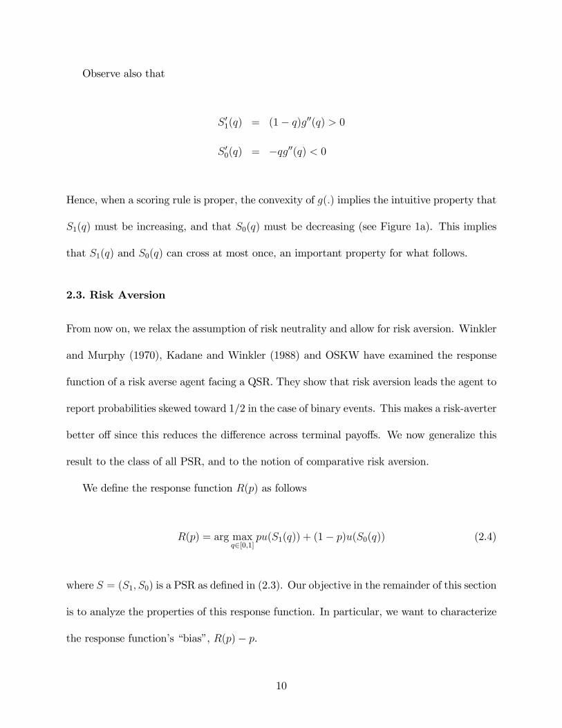
Observe also that

S 01(q) = (1� q)g00(q) > 0

S 00(q) = �qg00(q) < 0

Hence, when a scoring rule is proper, the convexity of g(:) implies the intuitive property that

S1(q) must be increasing, and that S0(q) must be decreasing (see Figure 1a). This implies

that S1(q) and S0(q) can cross at most once, an important property for what follows.

2.3. Risk Aversion

From now on, we relax the assumption of risk neutrality and allow for risk aversion. Winkler

and Murphy (1970), Kadane and Winkler (1988) and OSKW have examined the response

function of a risk averse agent facing a QSR. They show that risk aversion leads the agent to

report probabilities skewed toward 1/2 in the case of binary events. This makes a risk-averter

better o¤ since this reduces the di¤erence across terminal payo¤s. We now generalize this

result to the class of all PSR, and to the notion of comparative risk aversion.

We de�ne the response function R(p) as follows

R(p) = arg maxq2[0;1]

pu(S1(q)) + (1� p)u(S0(q)) (2.4)

where S = (S1; S0) is a PSR as de�ned in (2.3). Our objective in the remainder of this section

is to analyze the properties of this response function. In particular, we want to characterize

the response function�s �bias�, R(p)� p.

10

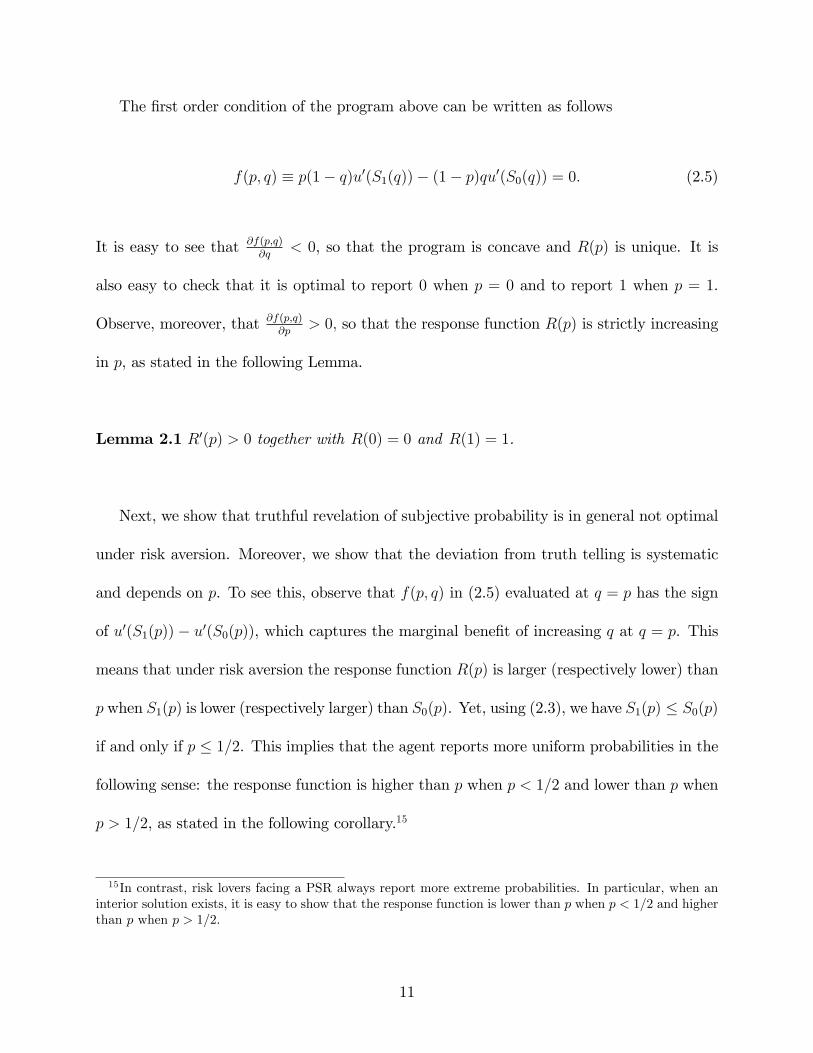
The �rst order condition of the program above can be written as follows

f(p; q) � p(1� q)u0(S1(q))� (1� p)qu0(S0(q)) = 0: (2.5)

It is easy to see that @f(p;q)@q

< 0, so that the program is concave and R(p) is unique. It is

also easy to check that it is optimal to report 0 when p = 0 and to report 1 when p = 1.

Observe, moreover, that @f(p;q)@p

> 0; so that the response function R(p) is strictly increasing

in p, as stated in the following Lemma.

Lemma 2.1 R0(p) > 0 together with R(0) = 0 and R(1) = 1.

Next, we show that truthful revelation of subjective probability is in general not optimal

under risk aversion. Moreover, we show that the deviation from truth telling is systematic

and depends on p. To see this, observe that f(p; q) in (2.5) evaluated at q = p has the sign

of u0(S1(p))� u0(S0(p)), which captures the marginal bene�t of increasing q at q = p. This

means that under risk aversion the response function R(p) is larger (respectively lower) than

p when S1(p) is lower (respectively larger) than S0(p). Yet, using (2.3), we have S1(p) � S0(p)

if and only if p � 1=2. This implies that the agent reports more uniform probabilities in the

following sense: the response function is higher than p when p < 1=2 and lower than p when

p > 1=2, as stated in the following corollary.15

15In contrast, risk lovers facing a PSR always report more extreme probabilities. In particular, when aninterior solution exists, it is easy to show that the response function is lower than p when p < 1=2 and higherthan p when p > 1=2.

11

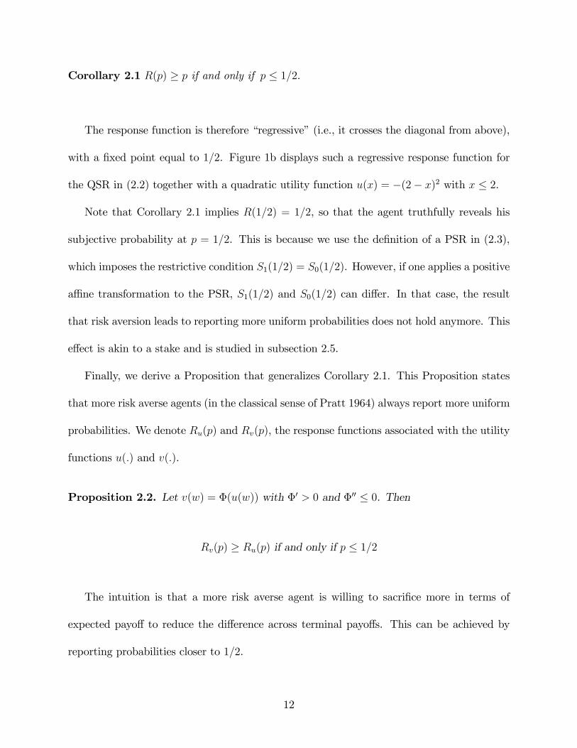
Corollary 2.1 R(p) � p if and only if p � 1=2.

The response function is therefore �regressive�(i.e., it crosses the diagonal from above),

with a �xed point equal to 1=2. Figure 1b displays such a regressive response function for

the QSR in (2.2) together with a quadratic utility function u(x) = �(2� x)2 with x � 2.

Note that Corollary 2.1 implies R(1=2) = 1=2, so that the agent truthfully reveals his

subjective probability at p = 1=2. This is because we use the de�nition of a PSR in (2.3),

which imposes the restrictive condition S1(1=2) = S0(1=2). However, if one applies a positive

a¢ ne transformation to the PSR, S1(1=2) and S0(1=2) can di¤er. In that case, the result

that risk aversion leads to reporting more uniform probabilities does not hold anymore. This

e¤ect is akin to a stake and is studied in subsection 2.5.

Finally, we derive a Proposition that generalizes Corollary 2.1. This Proposition states

that more risk averse agents (in the classical sense of Pratt 1964) always report more uniform

probabilities. We denote Ru(p) and Rv(p), the response functions associated with the utility

functions u(:) and v(:).

Proposition 2.2. Let v(w) = �(u(w)) with �0 > 0 and �00 � 0. Then

Rv(p) � Ru(p) if and only if p � 1=2

The intuition is that a more risk averse agent is willing to sacri�ce more in terms of

expected payo¤ to reduce the di¤erence across terminal payo¤s. This can be achieved by

reporting probabilities closer to 1=2.

12

2.4. Incentives

We now study the e¤ect of changing the incentives provided by the PSR. More precisely, we

study the e¤ect of changing a > 0 on the response function

R(p; a) = arg maxq2[0;1]

pu(aS1(q)) + (1� p)u(aS0(q)) (2.6)

We show that this e¤ect depends on the relative risk aversion coe¢ cient (x) = �xu00(x)u0(x) .

Proposition 2.3. Under 0(x) � (�)0,

@R(p; a)

@a� (�)0 if and only if p � 1=2.

In other words, under increasing (decreasing) relative risk aversion, an increase in the

rewards of the PSR leads the agent to report more (less) uniform probabilities. One can

present the intuition as follows. There are two e¤ects when the PSR payments increase: i) a

wealth e¤ect, as the agent gets a higher reward for any given reported probability, and ii) a

risk e¤ect, as the di¤erence between the rewards in the two states becomes more important.

The derivative of the relative risk aversion (x) ensures that one e¤ect always dominates the

other. In particular, when relative risk aversion is increasing, the risk e¤ect dominates the

wealth e¤ect so that the agent reports more uniform probabilities to reduce the variability

of her payo¤.16

An implication of this result is that, under constant relative risk aversion, changing the

PSR incentives has no e¤ect on the response function. As a result, it may not be possible

16Note that Proposition 2.3 relies on the assumption that initial wealth is equal to zero.

13

to mitigate the bias of the response function by adjusting the incentives of the PSR. In

particular, letting a tend to 0 does not guarantee that the response function R(p; a) tends to p

for all concave utility functions. Hence, the common belief that paying agents small amounts

induces risk-neutral behavior leading to truthful revelation is not correct in general.17

The result of Proposition 2.3 is illustrated in Figure 1c. The added response function

compared to Figure 1b is calculated for a = 2. Observe that both response functions are

regressive with a �xed point at 1=2. Yet, the increased incentives lead to reporting more

uniform probabilities. This is because the quadratic utility function used for the numerical

example displays increasing relative risk aversion.

2.5. Stakes

We now relax the �no-stake�condition by adding a constant to the reward S1 of the PSR.

We know that the PSR remains proper in this case since it is a simple positive a¢ ne transfor-

mation of the initial PSR. Moreover, observe that adding this constant is formally identical

to assuming that the agent�s wealth changes when the event obtains. We consider the latter

interpretation in the remainder of this section.

The response function is de�ned by

R(p;4) = arg maxq2[0;1]

pu(4+ S1(q)) + (1� p)u(S0(q)) (2.7)

in which the added reward 4 is a �nite (positive or negative) �stake�. The �rst order

17See, e.g., Kadane and Winkler (1988: 359) or Karni (1999: 480).

14

condition can be written

f(4; q) � p(1� q)u0(4+ S1(q))� (1� p)qu0(S0(q)) = 0 (2.8)

As before, @f(4;q)@q

< 0 under risk aversion, so that the program is concave. In addition, it is

immediate to see that the properties of Lemma 2.1 are still satis�ed. Finally, observe that

@f(4;q)@4 < 0 so that the response function is decreasing in 4 under risk aversion, as stated in

the following Lemma.

Lemma 2.2 @R(p;4)@4 � 0

The intuition for this result is straightforward. Under risk aversion, an increase in 4

reduces the marginal utility when the event occurs. Therefore, to compensate for the di¤er-

ence in marginal utility across states, the agent wants to increase the rewards of the PSR

when the event does not occur. This can be done by reducing the reported probability that

the event occurs. We can now state a Proposition that characterizes the response function

when the agent has a stake.

Proposition 2.4. The response function R(p;4) is characterized as follows:

i) if there exists a bp such that 4+ S1(bp) = S0(bp), then we haveR(p;4) � p if and only if p � bp

15

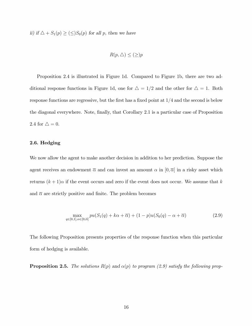
ii) if 4+ S1(p) � (�)S0(p) for all p, then we have

R(p;4) � (�)p

Proposition 2.4 is illustrated in Figure 1d. Compared to Figure 1b, there are two ad-

ditional response functions in Figure 1d, one for 4 = 1=2 and the other for 4 = 1. Both

response functions are regressive, but the �rst has a �xed point at 1=4 and the second is below

the diagonal everywhere. Note, �nally, that Corollary 2.1 is a particular case of Proposition

2.4 for 4 = 0.

2.6. Hedging

We now allow the agent to make another decision in addition to her prediction. Suppose the

agent receives an endowment � and can invest an amount � in [0; �] in a risky asset which

returns (k + 1)� if the event occurs and zero if the event does not occur. We assume that k

and � are strictly positive and �nite. The problem becomes

maxq2[0;1];�2[0;�]

pu(S1(q) + k�+ �) + (1� p)u(S0(q)� �+ �) (2.9)

The following Proposition presents properties of the response function when this particular

form of hedging is available.

Proposition 2.5. The solutions R(p) and �(p) to program (2.9) satisfy the following prop-

16

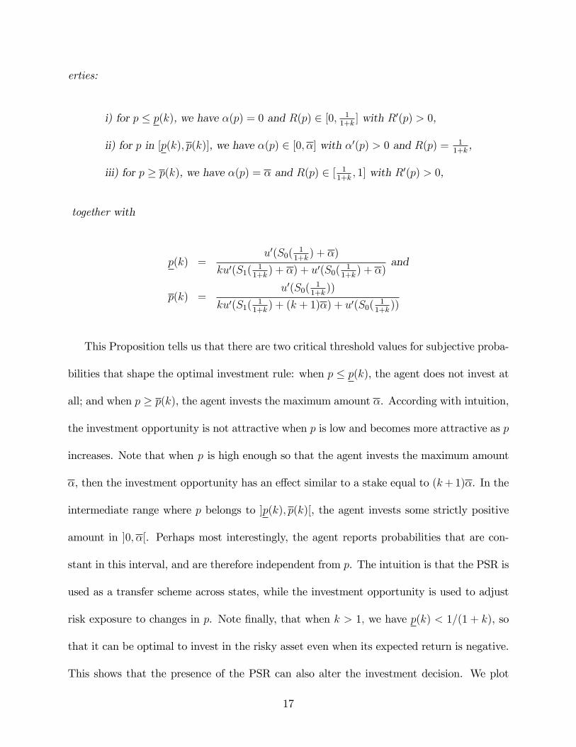
erties:

i) for p � p(k), we have �(p) = 0 and R(p) 2 [0; 11+k] with R0(p) > 0,

ii) for p in [p(k); p(k)], we have �(p) 2 [0; �] with �0(p) > 0 and R(p) = 11+k,

iii) for p � p(k), we have �(p) = � and R(p) 2 [ 11+k; 1] with R0(p) > 0,

together with

p(k) =u0(S0(

11+k) + �)

ku0(S1(11+k) + �) + u0(S0(

11+k) + �)

and

p(k) =u0(S0(

11+k))

ku0(S1(11+k) + (k + 1)�) + u0(S0(

11+k))

This Proposition tells us that there are two critical threshold values for subjective proba-

bilities that shape the optimal investment rule: when p � p(k), the agent does not invest at

all; and when p � p(k), the agent invests the maximum amount �. According with intuition,

the investment opportunity is not attractive when p is low and becomes more attractive as p

increases. Note that when p is high enough so that the agent invests the maximum amount

�, then the investment opportunity has an e¤ect similar to a stake equal to (k+1)�. In the

intermediate range where p belongs to ]p(k); p(k)[, the agent invests some strictly positive

amount in ]0; �[. Perhaps most interestingly, the agent reports probabilities that are con-

stant in this interval, and are therefore independent from p. The intuition is that the PSR is

used as a transfer scheme across states, while the investment opportunity is used to adjust

risk exposure to changes in p. Note �nally, that when k > 1; we have p(k) < 1=(1 + k), so

that it can be optimal to invest in the risky asset even when its expected return is negative.

This shows that the presence of the PSR can also alter the investment decision. We plot

17

in Figures 1e and 1f the optimal investment share �(p)=� and the response function under

k = 1 and � = 0:5.

3. Experimental Treatments

The main features of the experimental design are similar to OSKW�s (2009) calibration

experiment without explicit reference to beliefs or probability. The subjects are presented

with a list of 30 events, each describing the possible outcome of the roll of two 10-sided dice

(e.g. �the two dice sum up to 4�). Observe that, as in OSKW, each event has an objective

probability (i.e. it can be calculated using standard probability theory). Unlike OSKW,

however, the events in our experiment are not homogenous and consist of three di¤erent

series of 10 events. A precise description of the events and series is postponed to subsection

3.5.

For each of the 30 events, a subject is asked to make a choice consisting of selecting 1

out of 149 possible options called �choice numbers�. To each choice number correspond two

payments generated with a QSR. As further explained below, the �rst is the payment to the

subject when the event occurs, while the second is the payment to the subject when the event

does not occur. A subject�s set of possible choice numbers, as well as their corresponding

payments, was presented in the form of a �Choice Table�(see Appendix C).18 Observe that

the Choice Table is ordered such that, as the choice number increases, the payment when the

event occurs increases, while the payment when the event does not occur decreases. Note

also that the choice number 75 guarantees the same payment to a subject regardless of the

18How best to present PSR to subjects remains an open question. Tables, although not ideal, have beenoften adopted in part because they are simple to implement (see e.g. McKelvey and Page 1990, Sonnemansand O¤erman 2004, Rutström and Wilcox 2009, Blanco et al. 2009).

18

roll of the dice.

3.1. The Control Treatment

The subjects�payments in the control treatment (T0) are generated with a QSR of the form

S1(q) = a � [1� (1� q)2] and S0(q) = a � [1� q2], where a = 4; 000FCFA in our experiment.19

Each entry in the choice table, and in particular the link between choices and payments,

was explained in details and illustrated through several examples (see Appendix C). After

reading the instructions, the subjects�understanding of the table was submitted to a test,

which was then solved by the experimenter. The subjects were then presented with the list

of 30 events, one series at a time. No time limit was imposed, and the subjects could modify

any of their previous choices at any time.

Once all subjects had completed their task, the experimenter randomly selected one

of the 30 events and rolled the two dice once to determine whether this event occurred

or not. All subjects in a session was then paid according to their choice number for the

event randomly drawn. For instance, if a subject selects the choice number 30 for the event

randomly selected, she receives either 1,440 FCFA if the event obtains or 3,840 FCFA if the

event does not obtain (see Appendix C). This amount constitutes the entirety of a subject�s

payments, as no show-up fee was provided in the control treatment.

Based on the theoretical analysis conducted in the previous section, we can frame the

experimental hypotheses for each treatment in terms of the properties of the response func-

tion R(p). In particular, assuming subjects in our experiment are risk averse, we can use

Corollary 2.1 to formulate our �rst hypothesis.

19The Franc CFA is the currency used in Burkina Faso where the experiment was conducted (see Section3.6 for details). The conversion rate at the time was roughly $1 for 455 FCFA.

19

H0: The response function in T0 is i) regressive (i.e. it crosses the diagonal from above)

and ii) has a �xed point at 1=2.

3.2. The �High Incentives�and �Hypothetical Incentives�Treatments

Two treatments were conducted to study the e¤ect of incentives. As indicated in Table 1,

where the di¤erences between treatments are summarized, the �High Incentives�treatment

(T1) is identical to the control treatment except that every payment in the choice table is

now multiplied by 10. For instance, if a subject chose row 30, she received either 14,400

FCFA (instead of 1,440 FCFA in T0) if the event obtains or 38,400 FCFA (instead of 3,840

FCFA in T0) if the event does not obtain. The �Hypothetical Incentives� treatment (T2)

is identical to the �High Incentives�treatment except that payments are now hypothetical.

More speci�cally, subjects in T2 were asked to make their choices as if they would be paid

the amounts in the choice table. Yet, they knew they would receive only a �at fee of 3,000

FCFA for completing the task, regardless of their choices.

Proposition 2.3 shows that higher incentives a¤ect the response function only when rel-

ative risk aversion is non-constant. To derive a hypothesis, we follow most of the economic

literature (including recent papers on scoring rules such as OSKW or Andersen et al. 2009)

and assume constant relative risk aversion.

H1: The response function in T1 is identical to the response function in T0.

Since subjects�choices are not incentivized in T2, no theoretical prediction can be derived.

However, Holt and Laury (2002) suggest that treatments with high hypothetical payments

and treatment with low real payo¤s yield similar results. This leads to our next hypothesis.

20

H2: The response function in T2 is identical to the response function in T0.

3.3. The �Low Stake�and �High Stake�Treatments

Two treatments were conducted to study the e¤ect of stakes. These treatments are identical

to the control treatment except that subjects receive a bonus when the event occurs. The

bonus is 2,000 FCFA in the �Low Stake�treatment (T3) and 8,000 FCFA in the �High Stake�

treatment (T4).

Lemma 2.2 demonstrates that adding a positive stake when the event occurs lowers the

response function. Therefore, the response functions in T3 and T4 are predicted to be less

elevated everywhere than the response function in T0. Moreover, Proposition 2.4 identi�es

two special cases, one in which the response function is regressive with an interior �xed point

and one in which the response function is below the diagonal everywhere (and therefore has

no interior �xed point). It is easy to show, given the size of the stakes and the speci�c QSR

we used, that T3 corresponds to the �rst case with a �xed point at 1=4, while T4 corresponds

to the second case. This leads to the following hypotheses.

H3: The response function in T3 i) is lower than in T0 and ii) has a �xed point at 1=4.

H4: The response function in T4 i) is lower than in T3 and ii) is lower than p.

3.4. The �Low Hedging�and �High Hedging�Treatments

Two treatments were conducted to study the e¤ect of hedging. These treatments are identical

to the control treatment except that subjects are asked to make an additional decision for

each event. Namely, subjects were given 2; 000 FCFA and o¤ered the opportunity to bet a

share of this endowment. If the event does not occur, the bet is lost. If the event occurs, the

21

bet multiplied by 2 (respectively, 4) is paid to the subjects in the �Low Hedging�treatment

T5 (respectively, the �High Hedging�treatment T6). Finally, in both states of the world, the

subjects retain the part of the 2; 000 FCFA they did not bet. In other words, in addition to

selecting a choice number, subjects in the hedging treatments are asked to make a simple

portfolio decision with two assets, a riskless and a risky asset.

Proposition 2.5 shows that, with the possibility for hedging, the response function is

regressive, yet constant when the share of the endowment invested is in ]0,1[. Proposition

2.5 also shows that a subject invests all her endowment when p is high enough. In this case,

the hedging opportunity operates as a stake of 4; 000 FCFA (respectively, 8; 000 FCFA) in

treatment T5 (respectively, treatment T6), and the response functions are reduced accordingly

compared to T0. Observe �nally that T5 corresponds to the case k = 1 and T6 to the case

k = 3 in section 2.6. It is then easy to show that the �xed points in T5 and T6 are respectively

1=2 and 1=4. This leads to the following hypotheses:

H5: The response function in T5 is i) regressive with a �xed point at 1=2, ii) equal to 1=2

when the share invested is in ]0,1[, and iii) lower than in T0 when p is close to 1.

H6: The response function in T6 is i) regressive with a �xed point at 1=4, ii) equal to 1=4

when the share invested is in ]0,1[, and iii) lower than in T5 when p is close to 1.

3.5. Comparison of the Three Series

As mentioned previously, the 30 events presented to a subject had been split into 3 series of

10 events. In each series, the 10 events describe the possible outcome resulting from the roll

of two 10-sided dice (one black, the other red). To better compare a subject�s choices across

series, the 10 events in each series have the same objective probabilities 3%; 5%; 15%; 25%;

22

35%; 45%; 61%; 70%; 80%; and 90%. The events in Series 1 are similar to those in OSKW�s

calibration exercise. Namely, we told subjects that the red die determines the �rst digit and

the black die determines the second digit of a number between 1 and 100. For instance, we

described the event with an objective probability of 25% as �the number drawn is between 1

(included) and 25 (included)�. A complete description of the events and the order in which

they were presented to subjects may be found in Appendix C.

In Series 2, we consider events whose probabilities, although still objective, are arguably

more di¢ cult to calculate than those in Series 1. Namely, we told subjects that the two dice

would be added to form a number between 0 and 18. For instance, we described the event

with 25% probability as �the sum obtained is between 2 (included) and 6 (included)�.

The object of Series 3 is to test how subjects respond when faced with (objective) com-

pound probabilities. To do so, we asked subjects to select a single choice number not for

one but for two possible events. The subjects were told that the experimenter would throw

a fair coin to determine which of the two possible events would be taken into consideration

for payments. The events used in Series 3 are similar to those in Series 1, i.e. the roll of

the red and black dice produces a number between 1 and 100 and the events give a possible

range for that number. For instance, we described the event with a probability of 25% as

�If the coin falls on the Heads side, then the event is : "the number drawn is between 82

(included) and 89 (included)" ; otherwise, if the coin falls on the Tails side, then the event

is : "the number drawn is between 25 (included) and 66 (included)"�.

Since the objective probabilities are the same in each series, we expect no di¤erence

across the three series if subjects behave in a way consistent with expected utility based

on von Neumann Morgenstern axioms. Nevertheless, experimental evidence suggests that

23

subjects�responses may be a¤ected by the complexity in calculating objective probabilities.

In particular Halevy (2007) �nds that most subjects in his experiments do not reduce com-

pound probabilities. From a theoretical perspective, there are di¤erent ways to relax the

standard reduction axiom. We opted for a simple model of ambiguity recently introduced by

Klibano¤, Marinacci and Mukerji (2005) (KMM hereafter).20 Under this model, we show in

Proposition B.1 (see Appendix B) that, in the context of our experiment, ambiguity aversion

reinforces the e¤ect of risk aversion. As a result, the response functions obtained with Series

2 and 3 may be more biased than the response function obtained with Series 1. To derive a

hypothesis, however, we consider the standard expected utility approach.

H7: The response functions obtained in Series 1, 2, and 3 are identical.

3.6. Implementation of the Experiment

The experiment took place in Ouagadougou, Burkina Faso, in June 2009.21 The choice of

location was motivated by two factors. First, we wanted to take advantage of a favorable

exchange rate i) to create salient �nancial di¤erences between treatments (e.g. between the

reference and the �Hypothetical Incentives� treatments), and ii) to provide subjects with

substantial incentives so that risk aversion had a fair chance to play a role.22 Second, one

of the authors had conducted several experiments in Ouagadougou over the past three years

(see e.g. Armantier and Boly 2009, 2010). Building on our experience, we followed a well

established protocol to hire subjects and rent a lab to conduct the experiment.

20One reason for using this model is that KMM preferences enable one to distinguish ambiguity aversionfrom risk aversion. Also, Halevy (2007) �nds some support for these preferences.21Burkina Faso is a Francophone country in West Africa with over 13 million inhabitants, among which

around 1:4 million live in the capital city Ouagadougou.22The maximum payment of 40; 000 FCFA in the �High Incentives�treatment slightly exceeds the monthly

average entry salary for a university graduate.

24

More speci�cally, we used a local recruiting �rm (Opty-RH) to place �iers around Oua-

gadougou stating that we were looking for subjects for a paid economic experiment. The

subjects had to be at least 18 years old and be current or former university students. People

interested had to come to the recruiting �rm location with a proof of identi�cation and either

a valid university diploma or a proof of university enrollment. After their credentials were

validated, subjects were randomly assigned to a session and told when and where to show-up

for the experiment.

The sessions were conducted in a centrally located high school we had already rented in

the past to conduct other experiments. Upon arrival, the subjects were gathered in a large

room. The instructions were read aloud, followed by questions and a comprehension test.

The subjects were then presented with the 30 events and asked to make their choices using

pen and paper. Finally, the subjects �lled out a short survey, after which the experimenter

made the random draws and the subjects were paid in cash. Two sessions were conducted

for each treatment, with each session taking on average 90 minutes to complete.

As indicated in Table 2, a total of 301 subjects participated in the experiment, with a

minimum of 41 subjects per treatment. The subjects were composed mostly of men (74%)

and students currently enrolled at the university (68%), ranging in age between 19 and 38

(with a median age of 25). In the post-experiment survey, slightly more than half the subjects

reported having taken a probability or a statistics class at the university. Finally, most of

the subjects (86%) reported not having participated in a similar economic or psychology

experiment. Excluding the �Hypothetical Incentives�treatment (where earnings were �xed

at 3; 000 FCFA), the average earnings of a subject were 8; 861 FCFA. As indicated in Table

2, however, earnings varied greatly across subjects and treatments (the smallest amount paid

25

was 100 FCFA and the maximum was 40; 000 FCFA).

4. Experimental Results

4.1. The Control Treatment (T0)

Figure 2 shows the subjects�average responses to the events in the three series for each of

the 7 treatments conducted. According with hypothesis H0, the three response functions

in the control treatment are regressive. Moreover, they exhibit the traditional inverse S-

shape with a �xed point around 1=2. This observation is consistent with the literature, as

similar shapes have been previously identi�ed when eliciting beliefs (Huck and Weizsaker

2002, Sonnemans and O¤erman 2004, Hurley and Shogren 2005, OSKW). Figure 2 also

reveals that the three series can be ordered with respect to their respective biases. Indeed,

it appears that Series 1 (the simple probabilities) yields the smallest biases for virtually all

objective probabilities (i.e. Series 1�s response function is consistently the closest to the

diagonal), while Series 2 (the complex probabilities) generates the largest biases. This result

appears to contradict hypothesis H7 which states that under expected utility there should

be no systematic di¤erences across the three series.

To test our hypotheses more formally, we compare statistically the subjects�choices across

series and treatments with a parametric model of the form:

bPit = ' (Pt) + �i + uit (4.1)

where bPit is the reported probability corresponding to the choice number Nit selected by26

subject i for event t = 1; :::; 30 (i.e. bPit = 2=3 � Nit), Pt is the objective probability of

occurrence of event t, �i is a zero-mean normally distributed individual speci�c error term,

uit follows a normal distribution truncated such that bPit 2 [0; 1], and ' (:) is a continuousfunction satisfying ' (0) = 0, ' (1) = 1 and '0 (:) > 0. Consistent with previous literature,

we consider a function that may exhibit an inverse S-shape:

' (Pt) = exp�[lnPt]

b � [ln(a)]1�b�

(4.2)

where a 2]0; 1] and b > 0.

Observe that under the reparametrizationnb = �; a = exp

���

11��

�o, (4.2) is in fact the

probability weighting function w (Pt) = exp (�� [� lnPt]�) proposed in a di¤erent context

by Prelec (1998). The speci�cation in (4.2) was preferred to Prelec�s because the parameters

are easier to interpret with our experimental data. Indeed, observe that ' (a) = a and

'0 (a) = b. In other words, a captures where the function ' crosses the diagonal, while b

captures the slope of ' at this �xed point.23 Finally, we control for treatment and series

e¤ects by modeling the parameters in (4.2) as follows:

a = a0 + a1 � (S2 + S3) + a2 � S3 + a3 � T0 + a4 � T0 � (S2 + S3) + a5 � T0 � S3

where T0 is a dummy variable equal to 1 when the observation was collected in the control

treatment, while S2 and S3 are dummy variables equal to 1 when the event belongs respec-

tively to Series 2 and Series 3. The parameter b is modeled in an analog fashion. To estimate

23More generally, a captures the �elevation� of ' (:) and b captures its �curvature� (Gonzalez and Wu,1999). Indeed, assuming b < 1 so that '(:) is inverse S-shaped, then when a increases '(:) increases, whilewhen b increases '(:) increases if and only if p > a.

27

the model with the data collected only in the control treatment, the parameters a3 to a5, as

well as b3 to b5, are all set equal to zero. The parameters, estimated by Maximum Simulated

Likelihood, are reported in Table 4.

First, observe that in the control treatment a0 is not signi�cantly di¤erent from 1=2,

while b0 is signi�cantly smaller than 1. This therefore con�rms that the subjects�response

function for the events in Series 1 exhibits an inverse S-shape and crosses the diagonal near

1=2. Note also that a1 and a2 are not signi�cant in the control treatment. In other words,

the response functions��xed points do not appear to vary signi�cantly for the three series

in the control treatment. In contrast, b1 is signi�cantly smaller than 0, while b2 is positive

and signi�cant. This result con�rms that the curvature of the inverse S-Shape is the most

pronounced for the events in Series 2 and the least pronounced for the events in Series 1.

Observe also in Table 4 that the sign and signi�cance of (a1; a2), as well as (b1; b2), are

generally consistent across treatments. This therefore implies that the ranking of the three

series in terms of the biases they generate is generally preserved regardless of treatment.24

To gain a di¤erent perspective on the data, we calculate four statistics in Table 3. The

�rst is the average number of �extreme predictions�, that is, the average number of times

a subject selects a choice number below 10 (which corresponds to a reported probability

below 6:66%) or above 140 (which corresponds to a reported probability above 93:33%).

We also calculate two measures of the errors made by subjects when ranking the objective

probabilities. The �rst one (Error 1) consists of the average number of times a subject

incorrectly ranks two consecutive choice numbers with respect to their objective probabilities

24Similar conclusions can be reached nonparametrically using Friedman tests for each objective probabilityand series. Table 6 shows that in most treatments Series 1 (Series 2) generally has the lowest (highest) rankingof reported probabilities for objective probabilities below 50%, and the lowest (highest) ranking of reportedprobabilities for objective probabilities above 50%.

28

(e.g. the choice number selected by a subject for the objective probability 5% is higher than

the choice number he selected for the objective probability 15%). The second measure

captures the number of reported probabilities on the incorrect side of 1=2. More speci�cally,

�Error 2�consists of the average number of times a subject selects a choice number above

(below) 75 for an objective probability below (above) 50%. Finally, the choice numbers a

subject selects for a given objective probability are ordered across the three series from least

to most biased. We can see in Table 3 that these four criteria paint a consistent picture:

Series 1 (respectively, Series 2) has the most (least) extreme predictions, the fewest (most)

errors, and the best (worst) ranking in terms of bias. These results therefore provide further

support against the hypothesis that subjects respond similarly to the events in the three

series.

To summarize, we �nd statistical evidence that the response functions in the control

treatment exhibit the traditional inverse S-shape with a �xed point around 1=2. This result is

consistent with subjects being risk averse expected utility maximizers, and therefore supports

hypothesis H0. Moreover, we �nd that the responses to the events in Series 1 (Series 2) are

statistically the most (least) biased. This result cannot be explained under expected utility,

and therefore it contradicts hypothesis H7. Instead, the systematic di¤erences between

the three series can be rationalized by ambiguity aversion under the additional assumption

that Series 1 (the simple probabilities), Series 3 (the compound probabilities) and Series

2 (the complex probabilities) are ranked in increasing order of ambiguity. Arguably, this

assumption could �nd support in the fact that, although all objective, these three types

of probabilities (simple, compound, and complex) require di¤erent levels of computational

sophistication to calculate. In a recent paper, Halevy (2007) concludes that attitudes toward

29

ambiguity and compound objective lotteries are tightly associated. Our experimental results

not only support Halevy�s conclusion but also extend it by suggesting that complex objective

probabilities may also be perceived as ambiguous.25

4.2. The Incentives Treatments (T1 and T2)

Figure 2 indicates that the response functions for the three series in the �High Incentives�

treatment are �atter than in the control treatment, although they still cut the diagonal

around 1=2. This observation is con�rmed statistically in Table 4. Indeed, a3 to a5 are not

signi�cantly di¤erent from 0 in T1, thereby suggesting that the �xed points of the di¤er-

ent response functions cannot be distinguished statistically across the two treatments. In

contrast, we �nd the parameter b3 to be positive and signi�cant in T1. This con�rms that,

compared to the control treatment, the response functions are generally �atter in the �High

Incentive� treatment. Similar conclusions are reached nonparametrically by using Mann-

Whitney tests for each objective probability and each series. Indeed, Table 5 shows that for

most series and objective probabilities (except some objective probabilities around 1=2) the

distributions of responses in T1 are closer to the diagonal than in T0. Note also that the

the signs and magnitudes of b4 and b5 in Table 4 suggest that subjects�choices are more

homogenous across the three series in T1. This observation �nds additional support in the

criteria reported in Table 3. Indeed, responses to the events in Series 2 (Series 1) remain the

most (least) biased and the most (least) prone to errors, but the di¤erences across series are

not as severe as in T0.

25Our experiment also points out a potential problem with OSKW approach to correct for risk aversionwhen eliciting beliefs with a PSR: for the same agent, di¤erent correction functions could emerge in theircalibration exercise depending on the type of objective probabilities considered.

30

To sum up, responses in T1 are signi�cantly di¤erent from those in T0, which refutes

hypothesis H1 derived under the assumption of constant relative risk aversion. Instead, as

explained in Section 2:4, choices in T1 are consistent with subjects exhibiting increasing

relative risk aversion. In a recent paper, Andersen et al. (2009) also conclude that their

subjects�behavior in a similar belief elicitation experiment may be best described under

increasing relative risk aversion. It is also interesting to note that our results imply that

paying more does not necessarily yield �better� answers. Instead, we �nd that, because

of our subjects� speci�c form of relative risk aversion, using a PSR that provides higher

incentives generates more biases.

As for the �Hypothetical Incentives� treatment T2, Figure 2 reveals that subjects� re-

sponses, although still exhibiting the inverse S-shape, are on average closer to the diagonal

than in the control treatment. This observation is con�rmed statistically in Table 4 as b3

is found to be negative and signi�cant in T2. Note also that �u, the standard deviation of

the error term uit in (4.1), is signi�cantly larger for T2 than for T0. In addition, observe in

Table 3 that the number of extreme predictions and errors (of both forms) is systematically

greater in T2 than in T0. In other words, it appears that, although not as biased, subjects�

responses are noisier in the �Hypothetical Incentives�treatment. These results therefore do

not support hypothesis H2. Instead, we �nd that, when eliciting beliefs with a QSR, subjects

behave di¤erently when provided with real or hypothetical incentives. Our conclusions are

only partially consistent with the literature. Like Gachter and Renner (2006), we �nd that

�nancial incentives reduce the noise in the beliefs elicited. In contrast with our experiment,

however, Sonnemans and O¤erman (2004) �nd no di¤erence between rewarding predictors

with a QSR or with a �at fee.

31

4.3. The Treatments with Stakes (T3 and T4)

For the smallest objective probabilities, no obvious di¤erence is visible in Figure 2 between

the response functions in the control treatment and those in the low and high stakes treat-

ments. In contrast, Figure 2 clearly shows that, compared to T0, responses for the highest

objective probabilities are lower in T3 and lowest in T4. These observations are con�rmed

by the nonparametric tests in Table 5. There, we can see that the samples of responses for

each of the three series are stochastically lower in T0 for most objective probabilities above

25%. In addition, the comparison of the low and high stakes treatments in Table 5 indicates

that in general there exists a signi�cant di¤erence between the two treatments, whereby the

probabilities stated by subjects are generally lower in T4 than in T3. The parametric estima-

tions in Table 4 con�rm these results. Indeed, a3 and b3 are positive and signi�cant for both

treatments T3 and T4 but signi�cantly larger for treatment T4. This implies that, compared

to T0, the response functions become lower and �atter in the �Low Stake� treatment and

that the magnitude of this e¤ect is stronger in the �High Stake�treatment. In other words,

part i) of predictions H3 and H4 (i.e. the response functions are less elevated in T3 and T4)

is veri�ed. Behavior in the experiment, however, is not fully consistent with our predictions.

Indeed, observe in Table 4 that the parameter a3 is signi�cantly di¤erent from 1=4 in T3,

and from 0 in T4, thereby contradicting part ii) of H3 and H4.

To sum up, we �nd that when they have a stake in the event, subjects in our experiment

tend to smooth their payo¤s across the two states, especially when the event is likely to

occur. This treatment e¤ect is only partially in agreement with the theory: the direction is

correct, but the magnitude is insu¢ cient.

32

4.4. The Treatments with Hedging (T5 and T6)

The response functions for the two hedging treatments plotted in Figure 2 reveal several

di¤erences from those in the control treatment. First, for the highest objective probabilities,

the response functions become lower in T5 and lowest in T6. Second, although the �xed point

of the response function is also around 1=2 in T5, it is slightly above 40% in T6. Third, the

response functions appear slightly �atter (but not perfectly �at) around the diagonal in both

hedging treatments. Most of these observations are con�rmed statistically by the parametric

and nonparametric tests in Tables 4 and 5. In particular, observe in Table 4 that the estimate

of a3 is insigni�cant in T5, while it is positive and signi�cant in T6. The former is consistent

with part i) of hypothesis H5, as we cannot exclude that, as in the control treatment, the

response functions in the �Low Hedging�treatment cut the diagonal at 1=2. In the �High

Hedging�treatment, however, the parameter a0 is found to be signi�cantly greater than 1=4,

which contradicts part i) of hypothesis H6. Observe also that b3 is signi�cant and positive in

both T5 and T6, thereby indicating �atter responses around the diagonal in the two hedging

treatments compared to T0. The nonparametric tests in Table 5 also con�rm that, compared

to T0, responses for most objective probabilities above 60% are statistically lower in T5, and

lowest in T6. This result therefore supports part iii) of hypotheses H5 and H6.

Turning now to the subjects�betting behavior in the two hedging treatments, we can see

in Figure 2 that subjects in the �High Hedging� treatment invest more in the risky asset

for any objective probability than in the �Low Hedging� treatment. This observation is

con�rmed statistically by the nonparametric tests reported in the last column of Table 5.

The subjects�betting behavior, however, is not fully consistent with the theory. In particular,

33

we can see in Figure 2 that, on average, subjects invest strictly positive amounts even for low

probabilities, while they do not invest all of their endowments even for high probabilities.

To summarize, although not fully consistent with the theory, subjects in our experiment

appear to take partial advantage of their hedging opportunities. In particular, we �nd that

subjects tend to bet high on the most likely events, while simultaneously making lower

predictions than in the control treatment. In other words, it seems that subjects are willing

to take some risk on the bet, while using the scoring rule as an insurance in case the event

does not occur.

5. Discussion and Conclusion

Introduced in the 1950s by statisticians, Proper Scoring Rules (PSR) have arguably become

the most popular incentivized belief elicitation mechanism. In the simplest environment, a

well known result is that risk averters are better o¤ misreporting their beliefs by stating

more uniform probabilities (i.e. closer to 1/2 in the case of a binary event). Combining

theory and experiment, we �nd that this result does not generalize to richer environments

of particular interest to economists. Instead, we have shown that higher incentives, stakes,

and hedging may lead to severe distortions in reported probabilities.

We believe our results have implications for the elicitation of subjective probabilities

with PSR in general �eld settings. Indeed, as argued in the introduction, eliciting beliefs in

the �eld typically involves some form of stake or the possibility to hedge one�s prediction.

In particular, agents who participate in Prediction Markets based on PSR (the so called

Market Scoring Rule) always have a stake in the event they predict. In addition, as in our

34

experiment, the stakes in �eld environments are likely to be far larger than the prediction�s

reward. For instance, most prediction payments are likely to pale in comparison with the

stakes the agent may have in the stock market, a natural catastrophe, or the future of her

industry. Our results therefore suggest that in general �eld settings stakes and hedging are

likely to distort the beliefs reported with a PSR.

Moreover, the stakes and hedging opportunities an agent may have in the �eld are typi-

cally unobserved by the analyst. In such cases, theory cannot be used to predict and correct

the distortions generated by PSR. Suppose, nevertheless, that an agent has no stake in the

event she is predicting. Then, two additional issues arise. First, one may be concerned that

the beliefs elicited are not informative since the agent had no incentives ex-ante to acquire

information about the event. Second, one cannot rule out the possibility that the agent will

look for hedging opportunities ex-post. The presence of such opportunities may lead the

agent to bias her reported beliefs even though she has no stake when making her prediction.

In other words, (unobserved) stakes and hedging may lead to unpredictable distortions in

reported beliefs, thereby rendering PSR ine¤ective in recovering subjective probabilities in

general �eld environments.

Stakes and hedging may also play a role in lab experiments. Indeed, as argued in the

introduction, most individual decision making and strategic environments studied in experi-

mental economics involve one of these two e¤ects. Consistent with Blanco et al. (2010), our

results suggest that stakes and hedging can a¤ect both the beliefs elicited and the actions

taken in the experiment. This may explain why previous experiments found that i) some

subjects fail to best-respond to their stated beliefs (e.g. Costa-Gomez and Weizsaker 2008),

and ii) observers make di¤erent predictions about the play of a game than the subjects ac-

35

tually playing the game (e.g. Palfrey and Wang 2009). In contrast with the �eld, however,

the analyst has more control in the lab and possible remedial measures may be devised to

recover subjective beliefs when using a PSR. We now discuss the e¤ectiveness of some of

these remedial measures in the presence of stakes and hedging.

The method most frequently implemented in the lab to mitigate the e¤ect of risk aversion

on elicited beliefs consists in using a PSR that pays small amounts (e.g. Nyarko and Schotter

2002, Rutström and Wilcox 2009). Contrary to a widespread belief, however, this approach

may not be e¤ective in inducing more truthful reports. Instead, we have shown theoretically

that smaller payments can either accentuate or attenuate the PSR biases depending on the

agent�s relative risk aversion.

Recently, OSKW and Andersen et al. (2009) have independently proposed a di¤erent

approach to correct PSR biases in simple environments (i.e. without stakes or hedging).

Following (e.g.) Kadane and Winkler (1988), these �truth serums�are built on the premise

that if an agent�s primitives (e.g. utility, wealth) are known, then his optimal reported

probability can be calculated for any subjective probability. This function could then be

inverted to recover the agent�s unobserved beliefs from his stated probabilities. In OSKW,

relevant information is �rst collected in a calibration exercise to estimate this correction

function. This approach, however, tends to make belief elicitation with a PSR (an already

intrusive method) even more cumbersome. It is also unclear how this approach can be

generalized to economic environments with stakes and hedging.

Another well known remedial measure is to induce risk neutrality by paying agents in

lottery tickets that give them a chance to win a prize (Roth and Malouf 1979, Allen 1987,

Schlag and van der Weele 2009). In theory, it is easy to show that this approach is e¤ective

36

under expected utility in eliciting truthful beliefs as long as all payments (including the

stakes and hedging revenues) are made in lottery tickets. In practice, however, doubts have

been expressed about the ability of this approach to control for risk attitude (Davis and Holt

1993, Selten, Sadrieh and Abbink 1999). In addition, if the stake or hedging opportunity

arises from a task involving a risky choice (e.g. an investment or insurance decision), then

the analyst may not necessarily want to induce risk neutrality for that task.

A related approach when eliciting beliefs while playing a game consists in using random

draws to make the prediction and the game decision independent. For instance, Blanco et

al. (2010) propose to pay subjects randomly either their game or their prediction payo¤s.

Likewise, a subject in Armantier and Treich (2009) is randomly matched with two partners.

The subject plays the game against the �rst partner, and her prediction is scored against

the play of the second partner. Observe, however, that, although promising, the practical

e¤ectiveness of these methods remains mostly unproven.

To conclude, note that the adverse e¤ects of stakes and hedging are not speci�c to PSR.

It is easy to show that other incentivized belief elicitation techniques, although they may

o¤er some protection against risk aversion in the simplest environments, are not immune

to stakes and hedging. This is the case, for instance, for the standard lottery mechanism

(Kadane and Winkler, 1988) and for the direct revelation mechanism recently proposed

by Karni (2009). In fact, we are not aware of any incentivized belief elicitation method

that would directly address these issues.26 In this context, one may want to consider the

merits of eliciting beliefs without o¤ering any �nancial reward for accuracy. Although not

26Importantly, Karni and Safra (1995) show that unbiased belief elicitation is impossible when stakes arenot observed by the experimenter. This impossibility result holds even if the utility function is observableand even if several experiments can be implemented.

37

incentive compatible, this approach is simple, transparent, and commonly used in statistics,

psychology, and �eld surveys. In his review of the survey literature in economics, Manski

(2004) concludes that the beliefs elicited in such a way are informative. Our results support

this view and suggest that hypothetical payo¤s may be preferred if one is willing to trade

noise for unbiasedness.

6. References

Abramowicz, A., 2007, The hidden beauty of the quadratic scoring market rule: A uni-

form liquidity market maker, with variations, The Journal of Prediction Markets, 2, 111-125.

Allen, F., 1987, Discovering personal probabilities when utility functions are unknwown,

Management Science, 33, 542-44.

Andersen, S., Fountain, J., Harrison G.W. and E.E. Rutstrom, 2009, Estimating subjec-

tive probabilities, mimeo.

Armantier, O. and A. Boly, 2009, A controlled �eld experiment on corruption, working

paper, université de Montréal.

Armantier, O. and A. Boly, 2010, Can corruption be studied in the lab?, working paper,

université de Montréal.

Armantier, O. and N. Treich, 2009, Subjective probabilities in games: An application to

the overbidding puzzle, International Economic Review, 50, 1079-1102.

Beach, L.R. and L.D. Philips, 1967, Subjective probabilities inferred from estimates and

bets, Journal of Experimental Psychology, 75, 354-9.

Blanco, M.D., Engelmann, D., Koch A.K. and H.-T. Normann, 2010, Belief elicitation in

38

experiments: Is there a hedging problem?, mimeo.

Blinder A., Ehrmann M., Fratzscher M., De Haan J., and D. Jansen, 2008, Central bank

communication and monetary policy: A survey of theory and evidence, Journal of Economic

Literature, 46, 910�945.

Brier, G.W., 1950, Veri�cation of forecasts expressed in terms of probability, Monthly

Weather Review, 78, 1-3.

Bruine de BruinW., van der KlauwW., Downs J., Fischo¤B., Topa G. and O. Armantier,

2009, Expectations of in�ation: The role of �nancial literacy and demographic variables,

Journal of Consumer A¤airs, forthcoming.

Camerer, C.F., 1995, Individual decision making, In: Kagel, J.H. & Roth, A.E. (eds.):

Handbook of Experimental Economics, Princeton, NJ: Princeton University Press, 587-703.

Camerer, C.F. and R.M. Hogarth, 1999, The e¤ects of �nancial incentives in experiments:

A review and capital-labor-production framework, Journal of Risk and Uncertainty, 19, 7-42.

Costa-Gomez, M.A. and G. Weizsacker, 2008, Stated beliefs and play in normal-form

games, Review of Economic Studies, 75, 729-762.

Croson R., 2000, Thinking like a game theorist: Factors a¤ecting the frequency of equi-

librium play, Journal of Economic Behavior and Organization, 41, 299-314.

Davis, D. and C. Holt, 1993, Experimental Economics. Princeton, NJ: Princeton Uni-

versity Press.

De Finetti, B., 1981, The role of �dutch books� and �proper scoring rules�, British

Journal for the Philosophical of Science, 32, 55-56.

Fehr, D., Kübler, D. and D.N. Danz, 2009, Information and beliefs in a repeated normal-

form game, mimeo, Humboldt University, Berlin.

39

Fischbacher, U. and S. Gachter, 2008, Social preferences, beliefs, and the dynamics of

free riding in public good experiments, CESifo Working Paper No 2491.

Friedman, D., 1979, An e¤ective scoring rule for probability distributions, UCLA Eco-

nomics Working Papers 164.

Gachter, S. and E. Renner, 2006, The e¤ects of (incentivized) belief elicitation in public

good experiments, CeDEx Discussion Paper No. 2006�16.

Gneiting, T. and A.E. Raftery, 2007, Strictly proper scoring rules, prediction and esti-

mation, Journal of the American Statistical Association, 102, 359- 78.

Gonzalez, R. and G. Wu, 1999, On the shape of the probability weighting function,

Cognitive Psychology, 38, 129-66.

Good, I.J., 1952, Rational decisions, Journal of the Royal Statistical Society, Ser. B, 14,

107-14.

Halevy, Y., 2007, Ellsberg revisited: An experimental study, Econometrica, 75, 503-36.

Hanson, R., 2003, Combinatorial information market design, Information Systems Fron-

tiers, 5, 107-119.

Hertwig, R. and A. Ortmann, 2001, Experimental practices in economics: A methodolog-

ical challenge for psychologists?, Behavioral and Brain Sciences, 24, 383�451.

Holt, C, 1979, Elicitation of subjective probability distributions and von Neumann Mor-

genstern utility functions, University of Minnesota, Discussion Paper No. 79-128.

Holt, C.A. and S.K. Laury, 2002, Risk aversion and incentive e¤ects, American Economic

Review, 92, 1644-55.

Huck, S. and G. Weizsäcker, 2002, Do players correctly estimate what others do? Evi-

dence of conservatism in beliefs, Journal of Economic Behavior & Organization, 47, 71�85.

40

Hurley, T. and J. Shogren, 2005, An experimental comparison of induced and elicited

beliefs, The Journal of Risk and Uncertainty, 30, 169�188.

Kadane, J.B. and R.L. Winkler, 1988, Separating probability elicitation from utilities,

Journal of the American Statistical Association, 83, 357-63.

Karni, E., 1999, Elicitation of subjective probabilities when preference are state-dependent,

International Economic Review, 40, 479-486.

Karni, E., 2009, A mechanism for eliciting probabilities, Econometrica, 77, 603-06.

Karni, E. and Z. Safra, 1995, The impossibility of experimental elicitation of subjective

probabilities, Theory and Decision, 38, 313-320.

Kimball, A. W., 1951, On dependent tests of signi�cance in the analysis of variance, The

Annals of Mathematical Statistics, 22, 600-602.

Klibano¤, P., Marinacci M. and S. Mukerji, 2005, A smooth model of decision making

under ambiguity, Econometrica, 73, 1849-1892.

Ledyard, J.O., 2006, Designing information markets for policy analysis, in: Information

Markets: A New Way of Making Decisions, R.W. Hahn and P.C. Tetlock (editors), AEI-

Brookings Joint Center for Regulatory Studies.

Manski, C. F., 2002, Identi�cation of decision rules in experiments on simple games of

proposal and response, European Economic Review, 46, 880�891.

Manski, C. F., 2004, Measuring expectations, Econometrica, 72, 1329�1376.

McCarthy, J., 1956, Measures of the value of information, Proceedings of the National

Academy of Sciences, 654-5.

McKelvey, R.D. and T. Page, 1990, Public and private information: An experimental

study of information pooling, Econometrica, 58, 1321-39.

41

Nyarko, Y. and A. Schotter, 2002, An experimental study of belief learning using elicited

beliefs, Econometrica, 70, 971-1005.

O¤erman, T., Sonnemans, J., van de Kuilen, G. and P.P. Wakker, 2009, A truth-serum

for non-bayesians: Correcting proper scoring rules for risk attitudes, Review of Economics

Studies, 76, 1461-1489.

Osband, K., 1989, Optimal forecasting incentives, Journal of Political Economy, 97, 1091-

1112.

Ottaviani, M. and P.N. Sorensen, 2007, Outcome manipulation in corporate prediction

markets, Journal of the European Economic Association, 5, 554-63.

Palfrey, T.R. and S.W. Wang, 2009, On eliciting beliefs in strategic games, Journal of

Economic Behavior and Organization, 71, 2, 98-109.

Pratt, J. W., 1964, Risk aversion in the small and in the large, Econometrica, 32, 122-36.

Prelec, D., 1998, The probability weighting function, Econometrica, 66, 497-527.

Roth, A. E. and M. W. Malouf, 1979, Game-theoretic models and the role of information

in bargaining, Psychological Review, 86, 574�594

Rutström E. and N. Wilcox, 2009, Stated beliefs versus inferred beliefs: A methodological

inquiry and experimental test, 67, 2, 616-632.

Savage, L.J., 1971, Elicitation of personal probabilities and expectation, Journal of the

American Statistical Association, 66, 783-801.

Schervish, M.J., 1989, A general method for comparing probability assessors, The Annals

of Statistics, 17, 1856-1879.

Schlag K. and J. van der Weele, 2009, Eliciting probabilities, means, medians, variances

and covariances without assuming risk neutrality, mimeo.

42

Selten R., Sadrieh A. and K. Abbink, 1999, Money does not induce risk neutral behavior,

but binary lotteries do even worse, Theory and Decision, 46, 211-249.

Sonnemans J. and T. O¤erman, 2004, Is the quadratic scoring rule really incentive com-

patible?, mimeo, University of Amsterdam.

Wagner, A., 2009, Essays on the role of beliefs in economic decisions and interactions,

Ph. Dissertation, Toulouse School of Economics.

Winkler, R.L. and A.H. Murphy, 1970, Nonlinear utility and the probability score, Jour-

nal of Applied Meteorology, 9, 143-48.

Woodford M., 2005, Central bank communication and policy e¤ectiveness, Proceedings,

Federal Reserve Bank of Kansas City, August issue, 399-474.

43

0.2 0.4 0.6 0.8 1p

0.2

0.4

0.6

0.8

1

S0 S1

Figure 1a: Quadratic scoring rule

0.2 0.4 0.6 0.8 1p

0.2

0.4

0.6

0.8

1

optimal q

Figure 1b: Risk-aversion – response function

0.2 0.4 0.6 0.8 1p

0.2

0.4

0.6

0.8

1

optimal q

Figure 1c: Incentives – response functions 0.2 0.4 0.6 0.8 1

p

0.2

0.4

0.6

0.8

1

optimal q

Figure 1d: Stakes – response functions

0.2 0.4 0.6 0.8 1p

0.2

0.4

0.6

0.8

1

optimal α

Figure 1e: Hedging – share invested (bet)

0.2 0.4 0.6 0.8 1p

0.2

0.4

0.6

0.8

1

optimal q

Figure 1f: Hedging – response function

Simulations were done with Mathematica. Figure 1a represents a quadratic scoring rule (QSR): S1(q)=1-(1-q)2 and S0(q)=1-q2. Figures 1b, 1c and 1d represent the response functions under a QSR and a quadratic utility function: u(x)=-(2-x)2 with x≤2. Figure 1c represents the response functions for respective incentives a=1(plain curve) and a=2 (dashed curve). Figure 1d represents the response function for respective stakes D=0 (plain curve), D=½ (dashed curve) and D=1 (dashed curve, below the diagonal). Figures 1e and 1f represent respectively the optimal share invested (amount bet divided by maximal possible amount to bet) and the response function under a QSR, a quadratic utility function, a double-or-nothing investment opportunity (k=1) and a maximal possible amount to bet equal to 0.5.

Figure 1

20

30

40

50

60

70

80

90

100

jects` Average Response

T0  : Control Treatment 

Series 1 (Simple Proba)

Series 2 (Complex Proba)

Series 3 (compounded Proba)

80

90

100

ponse

T1  : High Incentives

80

90

100

ponse

T2  : Hypothetical Incentives

0

10

20

30

40

50

60

70

80

90

100

0 20 40 60 80 100

Subjects` Average Response

Objective Probability

T0  : Control Treatment 

Series 1 (Simple Proba)

Series 2 (Complex Proba)

Series 3 (compounded Proba)

0

10

20

30

40

50

60

70

80

90

100

0 20 40 60 80 100

Subjects` Average Response

Objective Probability

T1  : High Incentives

0

10

20

30

40

50

60

70

80

90

100

0 20 40 60 80 100Subjects` Average Response

Objective Probability

T2  : Hypothetical Incentives

0

10

20

30

40

50

60

70

80

90

100

0 20 40 60 80 100

Subjects` Average Response

Objective Probability

T0  : Control Treatment 

Series 1 (Simple Proba)

Series 2 (Complex Proba)

Series 3 (compounded Proba)

0

10

20

30

40

50

60

70

80

90

100

0 20 40 60 80 100

Subjects` Average Response

Objective Probability

T1  : High Incentives

0

10

20

30

40

50

60

70

80

90

100

0 20 40 60 80 100Subjects` Average Response

Objective Probability

T2  : Hypothetical Incentives

30

40

50

60

70

80

90

100

` Average Response

T3  : Low Stakes

30

40

50

60

70

80

90

100

` Average Response

T4  : High Stakes

0

10

20

30

40

50

60

70

80

90

100

0 20 40 60 80 100

Subjects` Average Response

Objective Probability

T0  : Control Treatment 

Series 1 (Simple Proba)

Series 2 (Complex Proba)

Series 3 (compounded Proba)

0

10

20

30

40

50

60

70

80

90

100

0 20 40 60 80 100

Subjects` Average Response

Objective Probability

T1  : High Incentives

0

10

20

30

40

50

60

70

80

90

100

0 20 40 60 80 100Subjects` Average Response

Objective Probability

T2  : Hypothetical Incentives

0

10

20

30

40

50

60

70

80

90

100

0 20 40 60 80 100

Subjects` Average Response

Objective Probability

T3  : Low Stakes

0

10

20

30

40

50

60

70

80

90

100

0 20 40 60 80 100

Subjects` Average Response

Objective Probability

T4  : High Stakes

80

90

100

ponse

T5  : Low Hedging (Response Function)

80

90

100

ponse

T6  : High Hedging (Response Function)

0

10

20

30

40

50

60

70

80

90

100

0 20 40 60 80 100

Subjects` Average Response

Objective Probability

T0  : Control Treatment 

Series 1 (Simple Proba)

Series 2 (Complex Proba)

Series 3 (compounded Proba)

0

10

20

30

40

50

60

70

80

90

100

0 20 40 60 80 100

Subjects` Average Response

Objective Probability

T1  : High Incentives

0

10

20

30

40

50

60

70

80

90

100

0 20 40 60 80 100Subjects` Average Response

Objective Probability

T2  : Hypothetical Incentives

0

10

20

30

40

50

60

70

80

90

100

0 20 40 60 80 100

Subjects` Average Response

Objective Probability

T3  : Low Stakes

0

10

20

30

40

50

60

70

80

90

100

0 20 40 60 80 100

Subjects` Average Response

Objective Probability

T4  : High Stakes

0

10

20

30

40

50

60

70

80

90

100

0 20 40 60 80 100

Subjects` Average Response

T5  : Low Hedging (Response Function)

0

10

20

30

40

50

60

70

80

90

100

0 20 40 60 80 100

Subjects` Average Response

T6  : High Hedging (Response Function)

0

10

20

30

40

50

60

70

80

90

100

0 20 40 60 80 100

Subjects` Average Response

Objective Probability

T0  : Control Treatment 

Series 1 (Simple Proba)

Series 2 (Complex Proba)

Series 3 (compounded Proba)

0

10

20

30

40

50

60

70

80

90

100

0 20 40 60 80 100

Subjects` Average Response

Objective Probability

T1  : High Incentives

0

10

20

30

40

50

60

70

80

90

100

0 20 40 60 80 100Subjects` Average Response

Objective Probability

T2  : Hypothetical Incentives

0

10

20

30

40

50

60

70

80

90

100

0 20 40 60 80 100

Subjects` Average Response

Objective Probability

T3  : Low Stakes

0

10

20

30

40

50

60

70

80

90

100

0 20 40 60 80 100

Subjects` Average Response

Objective Probability

T4  : High Stakes

0

10

20

30

40

50

60

70

80

90

100

0 20 40 60 80 100

Subjects` Average Response

Objective Probability

T5  : Low Hedging (Response Function)

0

10

20

30

40

50

60

70

80

90

100

0 20 40 60 80 100

Subjects` Average Response

Objective Probability

T6  : High Hedging (Response Function)

30

40

50

60

70

80

90

100

` Average Bet (in %)

T5  : Low Hedging (Bets)

30

40

50

60

70

80

90

100

` Average Bet (in %)

T6  : High Hedging (Bets)

0

10

20

30

40

50

60

70

80

90

100

0 20 40 60 80 100

Subjects` Average Response

Objective Probability

T0  : Control Treatment 

Series 1 (Simple Proba)

Series 2 (Complex Proba)

Series 3 (compounded Proba)

               Figure 2

0

10

20

30

40

50

60

70

80

90

100

0 20 40 60 80 100

Subjects` Average Response

Objective Probability

T1  : High Incentives

0

10

20

30

40

50

60

70

80

90

100

0 20 40 60 80 100Subjects` Average Response

Objective Probability

T2  : Hypothetical Incentives

0

10

20

30

40

50

60

70

80

90

100

0 20 40 60 80 100

Subjects` Average Response

Objective Probability

T3  : Low Stakes

0

10

20

30

40

50

60

70

80

90

100

0 20 40 60 80 100

Subjects` Average Response

Objective Probability

T4  : High Stakes

0

10

20

30

40

50

60

70

80

90

100

0 20 40 60 80 100

Subjects` Average Response

Objective Probability

T5  : Low Hedging (Response Function)

0

10

20

30

40

50

60

70

80

90

100

0 20 40 60 80 100

Subjects` Average Response

Objective Probability

T6  : High Hedging (Response Function)

0

10

20

30

40

50

60

70

80

90

100

0 20 40 60 80 100

Subjects` Average Bet (in %)

Objective Probability

T5  : Low Hedging (Bets)

0

10

20

30

40

50

60

70

80

90

100

0 20 40 60 80 100

Subjects` Average Bet (in %)

Objective Probability

T6  : High Hedging (Bets)

0

10

20

30

40

50

60

70

80

90

100

0 20 40 60 80 100

Subjects` Average Response

Objective Probability

T0  : Control Treatment 

Series 1 (Simple Proba)

Series 2 (Complex Proba)

Series 3 (compounded Proba)

Table 1 : Financial Differences between Treatments (in FCFA) T0

Control

T1 High

Incentives

T2 Hypothetical

Incentives

T3 Low

Stakes

T4 High

Stakes

T5 Low

Hedging

T6 High

Hedging Show-up-fee 0 0 3,000 0 0 0 0

Maximum Scoring Rule Payment 4,000 40,000 0 4,000 4,000 4,000 4,000 Stakes 0 0 0 2,000 8,000 0 0

Maximum Return on Investment 0 0 0 0 0 4,000 8,000  

Table 2 : Characteristics of the Subject Pool T0

Control

T1 High

Incentives

T2 Hypothetical

Incentives

T3 Low

Stakes

T4 High

Stakes

T5 Low

Hedging

T6 High

HedgingNumber of Subjects 43 43 48 41 44 41 41

Age 24.581 (2.373)

25.119 (2.350)

24.208 (2.042)

24.350 (2.315)

25.605 (2.977)

24.850 (3.286)

25.475 (2.792)

% of Female 27.9% 23.8% 25.0% 29.3% 23.3% 25.0% 29.3% % Currently Enrolled at the University 67.2% 64.5% 71.6% 70.5% 60.8% 68.0% 61.5%

% with University Course in Probability 60.0% 52.8% 54.2% 61.0% 57.5% 50.0% 53.7% % with Previous Participation in Experiment 14.6% 15.0% 16.7% 9.8% 20.9% 15.4% 12.2%

Subjects’ average Earnings 3,055.2 (1,565.5)

28,341.8 (8,121.7)

3,000 (__)

5,277.3 (1,173.2)

7,864.9 (4,189.5)

4,992.8 (1,226.3)

6,155.8 (1,583.9)

Table 3 : Features of Subjects’ Responses

Series T0

Control

T1 High

Incentives

T2 Hypothetical Incentives

T3 Low

Stakes

T4 High

Stakes

T5 Low

Hedging

T6 High

Hedging

Extreme

Prediction1

S1 1.070 (0.985)

0.023 (0.152)

2.116 (1.531)

1.148 (1.236)

0.977 (1.000)

1.122 (1.166)

1.244 (1.985)

S2 0.558 (0.796)

0.093 (0.366)

1.465 (1.120)

0.415 (0.774)

0.864 (1.268)

0.439 (0.808)

0.780 (2.019)

S3 0.721 (0.959)

0.070 (0.258)

1.488 (1.470)

0.902 (0.944)

0.932 (1.208)

0.683 (1.059)

1.000 (1.987)

Error 12

S1 1.093 (0.947)

0.953 (1.045)

1.698 (1.301)

1.049 (0.973)

0.955 (0.861)

1.171 (1.093)

1.049 (0.973)

S2 1.744 (1.157)

1.465 (1.437)

2.349 (1.066)

1.683 (0.934)

1.727 (1.169)

1.878 (1.364)

1.439 (1.285)

S3 1.395 (1.158)

1.209 (1.186)

2,372 (1.047)

1.537 (1.247)

1.409 (1.085)

1.488 (0.952)

1.293 (1.123)

Error 23

S1 0.419 (0.626)

0.372 (0.655)

0.605 (0.760)

0.634 (0.733)

0.932 (1.087)

0.537 (0.636)

0.878 (1.345)

S2 0.767 (0.947)

0.674 (0.919)

1.163 (0.998)

0.878 (0.872)

1.523 (1.191)

0.683 (0.960)

1.220 (1.475)

S3 0.674 (0.680)

0.372 (0.725)

1.163 (0.924)

0.805 (0.782)

1.227 (1.309)

0.390 (0.737)

1.073 (1.403)

Series

Ranking4

S1 1.515 (0.669)

1.828 (0.629)

1.795 (0.721)

1.732 (0.254)

1.748 (0.694)

1.793 (0.251)

1.741 (0.263)

S2 2.398 (0.724)

2.112 (0.712)

2.091 (0.792)

2.318 (0.250)

2.255 (0.731)

2.220 (0.242)

2.310 (0.241)

S3 2.087 (0.708)

2.060 (0.676)

2.114 (0.783)

1.950 (0.292)

1.998 (0.717)

1.988 (0.257)

1.949 (0.228)

In each cell, the first number is the average per subject, while the number in parenthesis is the standard deviation. 1 For each subject and each Series, “Extreme Prediction” captures the number of time his choice number is below 10 or above 140. 2 For each subject and each Series, “Error 1” captures the number of time his choice numbers are incorrectly ordered (e.g. In Series 1, the choice number associated with the 5% probability event is greater than the choice number associated with the 15% probability event). 3 For each subject and each Series, “Error 2” captures the number of time a choice number above 75 is selected for an event with probability below 50%, plus the number of time a choice number below 75 is selected for an event with probability above 50%. 4 For each subject and each of the 10 objective probabilities, the three series are ranked from least to most biased. “Series Ranking” therefore equals to 1, 2 or 3, depending on that ranking.

 

 

 

 

 

 

 

Table 4 : Estimation of the Response Function T0

Control

T1 High

Incentives

T2 Hypothetical

Incentives

T3 Low

Stakes

T4 High

Stakes

T5 Low

Hedging

T6 High

Hedging

0.480*** (0.024)

0.501*** (0.006)

0.499*** (0.156)

0.425*** (0.016)

0.393*** (0.032)

0.493*** (0.012)

0.402*** (0.029)

0.026 (0.021)

0.004 (0.005)

-0.018 (0.016)

0.019 (0.013)

0.006 (0.014)

-0.024 (0.016)

0.013 (0.013)

0.004 (0.011)

-0.002 (0.006)

-0.020 (0.043)

2.851E-4 (0.014)

-0.007 (0.012)

0.009 (0.013)

-0.010 (0.008)

__ -0.034

(0.023) -0.038 (0.059)

0.048** (0.023)

0.109*** (0.040)

-0.031 (0.029)

0.101*** (0.035)

· __ 0.020

(0.020) 0.047

(0.048) 0.005

(0.024) 0.003

(0.031) 0.052* (0.028)

-0.009 (0.023)

· __ 0.008

(0.013) 0.024

(0.045) 0.004

(0.017) 0.015

(0.016) -0.005 (0.017)

0.025* (0.014)

0.736*** (0.054)

0.289*** (0.033)

0.901*** (0.060)

0.622*** (0.037)

0.518*** (0.038)

0.543*** (0.057)

0.499*** (0.040)

-0.242*** (0.029)

-0.053*** (0.015)

-0.195*** (0.043)

-0.189*** (0.025)

-0.119*** (0.024)

-0.210*** (0.032)

-0.157*** (0.017)

0.067*** (0.021)

0.009 (0.013)

0.015 (0.035)

0.129*** (0.024)

0.056** (0.026)

0.086*** (0.024)

0.072*** (0.013)

__ 0.434***

(0.061) -0.147** (0.068)

0.107** (0.051)

0.222*** (0.071)

0.207** (0.083)

0.197*** (0.062)

· __ -0.179***

(0.032) -0.058 (0.055)

-0.048 (0.039)

-0.103** (0.042)

-0.042 (0.046)

-0.049 (0.031)

· __ 0.055

(0.034) 0.052

(0.042) -0.063 (0.042)

0.012 (0.036)

-0.017 (0.035)

-0.010 (0.024)

0.020*** (0.004)

0.024*** (0.003)

0.029*** (0.003)

0.026*** (0.005)

0.093*** (0.017)

0.025*** (0.003)

0.114*** (0.015)

0.107*** (0.006)

0.097*** (0.003)

0.133*** (0.004)

0.101*** (0.003)

0.106*** (0.004)

0.117*** (0.004)

0.103*** (0.004)

ln -2602.37 -5362.18 -5532.78 -5165.09 -5220.24 -4832.89 -4937.02 In each cell, the first number corresponds to the point estimate, while the number in parenthesis is the estimated standard deviation of the parameter. ***, **, and * respectively indicate parameters significant at the 1%, 5% and 10% levels.

 

 

 

 

 

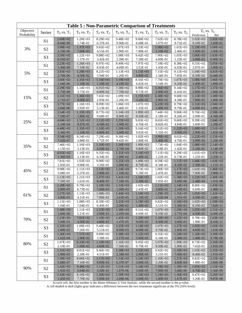
Table 5 : Non-Parametric Comparison of Treatments Objective

Probability

Series

T0 vs. T1

T0 vs. T2

T0 vs. T3

T0 vs. T4

T3 vs. T4

T0 vs. T5

T0 vs. T6 T5 vs. T6 Prediction Bet

3%

S1 2.60E+02 1.20E+03 8.29E+02 9.48E+02 9.60E+02 7.02E+02 8.78E+02 1.02E+03 5.92E+02 8.64E-09 1.74E-01 6.37E-01 9.90E-01 6.08E-01 1.07E-01 9.71E-01 9.10E-02 1.60E-02

S2 3.98E+02 1.37E+03 9.65E+02 1.07E+03 9.33E+02 5.98E+02 1.01E+03 1.19E+03 5.00E+02 5.19E-06 7.00E-03 4.55E-01 2.90E-01 7.88E-01 1.10E-02 2.40E-01 1.00E-03 1.00E-03

S3 3.50E+02 1.22E+03 9.88E+02 1.08E+03 9.42E+02 7.90E+02 1.05E+03 1.06E+03 5.63E+02 6.55E-07 1.37E-01 3.42E-01 2.39E-01 7.28E-01 4.09E-01 1.23E-01 3.90E-02 6.00E-03

5%

S1 2.23E+02 1.26E+03 8.97E+02 8.49E+02 7.97E+02 7.18E+02 8.38E+02 9.55E+02 5.05E+02 1.30E-09 7.10E-02 8.93E-01 4.09E-01 3.52E-01 1.43E-01 6.93E-01 2.87E-01 1.00E-03

S2 3.83E+02 1.28E+03 8.22E+02 1.13E+03 1.13E+03 7.15E+02 9.12E+02 1.04E+03 4.41E+02 2.70E-06 4.50E-02 5.94E-01 1.26E-01 4.80E-02 1.34E-01 7.85E-01 6.50E-02 6.44E-05

S3 3.60E+02 1.35E+03 1.16E+03 1.19E+03 8.56E+02 7.78E+02 1.07E+03 1.08E+03 3.96E+02 1.04E-06 1.10E-02 1.20E-02 4.10E-02 6.82E-01 3.54E-01 9.20E-02 2.40E-02 1.89E-05

15%

S1 2.29E+02 1.14E+03 6.91E+02 7.38E+02 8.98E+02 5.36E+02 9.34E+02 1.17E+03 3.37E+02 1.73E-09 3.75E-01 8.80E-02 7.70E-02 9.72E-01 2.00E-03 6.41E-01 2.00E-03 1.96E-06

S2 3.31E+02 1.36E+03 7.65E+02 1.09E+03 1.15E+03 6.38E+02 9.68E+02 1.13E+03 3.38E+02 2.71E-07 9.00E-03 2.95E-01 2.26E-01 3.20E-02 2.90E-02 4.38E-01 7.00E-03 1.80E-06

S3 3.77E+02 1.16E+03 8.09E+02 1.06E+03 1.07E+03 5.22E+02 8.79E+02 1.15E+03 2.94E+02 2.04E-06 2.92E-01 5.13E-01 3.46E-01 1.35E-01 1.00E-03 9.79E-01 4.00E-03 1.89E-07

25%

S1 3.54E+02 1.33E+03 8.77E+02 1.14E+03 1.09E+03 7.44E+02 9.06E+02 9.76E+02 2.58E+02 7.59E-07 1.80E-02 9.68E-01 9.90E-02 9.50E-02 2.18E-01 8.26E-01 2.09E-01 4.34E-08

S2 4.84E+02 1.52E+03 1.11E+03 1.25E+03 9.83E+02 8.65E+02 9.60E+02 9.39E+02 2.84E+02 1.24E-04 9.87E-05 4.50E-02 1.00E-02 4.76E-01 8.82E-01 4.84E-01 3.60E-01 1.29E-07

S3 4.48E+02 1.35E+03 1.10E+03 1.20E+03 9.16E+02 9.51E+02 1.22E+03 1.08E+03 2.51E+02 3.36E-05 1.10E-02 4.80E-02 3.00E-02 9.02E-01 5.32E-01 3.00E-03 2.90E-02 1.83E-08

35%

S1 3.54E+02 9.24E+02 7.29E+02 9.38E+02 1.02E+03 3.99E+02 8.02E+02 1.22E+03 2.25E+02 7.02E-07 3.88E-01 1.72E-01 9.42E-01 2.88E-01 1.46E-05 4.76E-01 3.98E-04 5.29E-09

S2 7.46E+02 1.16E+03 1.10E+03 1.36E+03 1.09E+03 7.73E+02 1.04E+03 1.08E+03 2.14E+02 1.13E-01 3.13E-01 4.50E-02 3.70E-04 9.80E-02 3.18E-01 1.42E-01 2.10E-02 3.14E-09

S3 4.95E+02 1.16E+03 9.35E+02 1.25E+03 1.16E+03 7.11E+02 9.29E+02 1.01E+03 1.47E+02 1.36E-04 3.13E-01 6.34E-01 1.00E-02 2.40E-02 1.22E-01 6.73E-01 1.22E-01 5.35E-11

45%

S1 7.81E+02 1.03E+03 9.90E+02 1.25E+03 1.09E+03 8.59E+02 1.11E+03 1.08E+03 1.63E+02 1.95E-01 9.90E-01 3.26E-01 1.00E-02 8.70E-02 8.34E-01 4.20E-02 2.50E-02 1.21E-10

S2 9.98E+02 1.11E+03 1.12E+03 1.24E+03 9.73E+02 1.00E+03 1.17E+03 1.02E+03 1.46E+02 5.08E-01 5.37E-01 2.80E-02 1.10E-02 5.28E-01 2.47E-01 7.00E-03 7.00E-02 3.90E-11

S3 1.12E+03 1.21E+03 1.07E+03 1.41E+03 1.16E+03 1.02E+03 1.38E+03 1.22E+03 2.40E+02 7.50E-02 1.61E-01 8.40E-02 7.18E-05 2.30E-02 2.05E-01 5.68E-06 2.48E-04 1.01E-08

61%

S1 1.28E+03 9.79E+02 1.18E+03 1.33E+03 1.03E+03 1.11E+03 1.14E+03 8.86E+02 1.43E+02 2.00E-03 6.73E-01 7.00E-03 1.00E-03 2.43E-01 3.80E-02 2.10E-02 6.69E-01 1.48E-11

S2 1.27E+03 1.13E+03 1.08E+03 1.44E+03 1.16E+03 1.29E+03 1.35E+03 1.05E+03 1.42E+02 3.00E-03 4.31E-01 7.80E-02 2.63E-05 2.10E-02 2.52E-04 1.91E-05 4.50E-02 2.68E-11

S3 1.11E+03 1.08E+03 8.59E+02 1.22E+03 1.18E+03 9.82E+02 1.16E+03 1.02E+03 1.59E+02 1.04E-01 7.04E-01 8.40E-01 2.00E-02 1.40E-02 3.51E-01 1.30E-02 8.20E-02 7.82E-11

70%

S1 1.48E+03 1.11E+03 1.23E+03 1.38E+03 9.51E+02 1.07E+03 1.29E+03 1.05E+03 2.51E+02 1.60E-06 5.21E-01 2.00E-03 2.45E-04 6.69E-01 9.10E-02 2.71E-04 4.50E-02 6.00E-09

S2 1.23E+03 7.81E+02 1.10E+03 1.45E+03 1.20E+03 1.10E+03 1.22E+03 9.78E+02 1.63E+02 7.00E-03 4.50E-02 4.80E-02 1.47E-05 9.00E-03 4.50E-02 3.00E-03 1.98E-01 8.45E-11

S3 1.32E+03 1.08E+03 9.48E+02 1.25E+03 1.14E+03 1.07E+03 1.27E+03 1.05E+03 2.65E+02 1.00E-03 7.26E-01 5.51E-01 9.00E-03 4.00E-02 9.70E-02 1.00E-03 4.60E-02 1.65E-08

80%

S1 1.36E+03 7.57E+02 9.89E+02 1.38E+03 1.22E+03 9.35E+02 1.24E+03 1.10E+03 3.30E+02 1.62E-04 2.90E-02 3.38E-01 2.57E-04 5.00E-03 6.34E-01 1.00E-03 1.40E-02 8.78E-08

S2 1.07E+03 6.33E+02 1.10E+03 1.16E+03 9.05E+02 1.07E+03 1.09E+03 8.73E+02 2.16E+02 2.19E-01 1.00E-03 4.60E-02 7.50E-02 9.79E-01 9.50E-02 5.90E-02 7.65E-01 1.91E-09

S3 1.31E+03 8.81E+02 9.66E+02 1.38E+03 1.25E+03 9.92E+02 1.18E+03 1.03E+03 2.35E+02 1.00E-03 2.28E-01 4.51E-01 2.34E-04 2.00E-03 3.21E-01 7.00E-03 8.40E-02 1.91E-09

90%

S1 1.50E+03 8.06E+02 1.17E+03 1.53E+03 1.24E+03 1.10E+03 1.27E+03 9.82E+02 3.15E+02 5.68E-07 7.10E-02 9.00E-03 6.37E-07 3.00E-03 5.20E-02 4.60E-04 1.88E-01 2.66E-08

S2 1.42E+03 9.48E+02 1.12E+03 1.51E+03 1.24E+03 1.18E+03 1.39E+03 1.05E+03 2.55E+02 1.92E-05 5.04E-01 3.50E-02 1.87E-06 3.00E-03 7.00E-03 5.68E-06 4.70E-02 5.56E-09

S3 1.43E+03 8.10E+02 1.20E+03 1.50E+03 1.24E+03 1.24E+03 1.36E+03 9.47E+02 3.26E+02 1.45E-05 7.70E-02 5.00E-03 2.69E-06 3.00E-03 1.00E-03 1.67E-05 3.20E-01 9.87E-08

In each cell, the first number is the Mann-Whitney U Test Statistic, while the second number is the p-value. A cell shaded in dark (light) gray indicates a difference between the two treatments significant at the 5% (10% level).

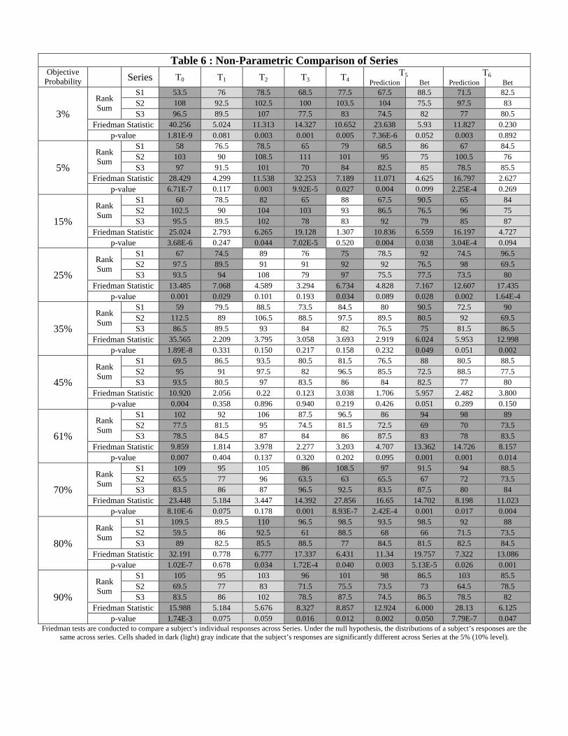
Table 6 : Non-Parametric Comparison of Series Objective

Probability

Series T0 T1 T2 T3 T4 T5 T6 Prediction Bet Prediction Bet

3% Rank Sum

S1 53.5 76 78.5 68.5 77.5 67.5 88.5 71.5 82.5 S2 108 92.5 102.5 100 103.5 104 75.5 97.5 83 S3 96.5 89.5 107 77.5 83 74.5 82 77 80.5

Friedman Statistic 40.256 5.024 11.313 14.327 10.652 23.638 5.93 11.827 0.230 p-value 1.81E-9 0.081 0.003 0.001 0.005 7.36E-6 0.052 0.003 0.892

5% Rank Sum

S1 58 76.5 78.5 65 79 68.5 86 67 84.5 S2 103 90 108.5 111 101 95 75 100.5 76 S3 97 91.5 101 70 84 82.5 85 78.5 85.5

Friedman Statistic 28.429 4.299 11.538 32.253 7.189 11.071 4.625 16.797 2.627 p-value 6.71E-7 0.117 0.003 9.92E-5 0.027 0.004 0.099 2.25E-4 0.269

15% Rank Sum

S1 60 78.5 82 65 88 67.5 90.5 65 84 S2 102.5 90 104 103 93 86.5 76.5 96 75 S3 95.5 89.5 102 78 83 92 79 85 87

Friedman Statistic 25.024 2.793 6.265 19.128 1.307 10.836 6.559 16.197 4.727 p-value 3.68E-6 0.247 0.044 7.02E-5 0.520 0.004 0.038 3.04E-4 0.094

25% Rank Sum

S1 67 74.5 89 76 75 78.5 92 74.5 96.5 S2 97.5 89.5 91 91 92 92 76.5 98 69.5 S3 93.5 94 108 79 97 75.5 77.5 73.5 80

Friedman Statistic 13.485 7.068 4.589 3.294 6.734 4.828 7.167 12.607 17.435 p-value 0.001 0.029 0.101 0.193 0.034 0.089 0.028 0.002 1.64E-4

35% Rank Sum

S1 59 79.5 88.5 73.5 84.5 80 90.5 72.5 90 S2 112.5 89 106.5 88.5 97.5 89.5 80.5 92 69.5 S3 86.5 89.5 93 84 82 76.5 75 81.5 86.5

Friedman Statistic 35.565 2.209 3.795 3.058 3.693 2.919 6.024 5.953 12.998 p-value 1.89E-8 0.331 0.150 0.217 0.158 0.232 0.049 0.051 0.002

45% Rank Sum

S1 69.5 86.5 93.5 80.5 81.5 76.5 88 80.5 88.5 S2 95 91 97.5 82 96.5 85.5 72.5 88.5 77.5 S3 93.5 80.5 97 83.5 86 84 82.5 77 80

Friedman Statistic 10.920 2.056 0.22 0.123 3.038 1.706 5.957 2.482 3.800 p-value 0.004 0.358 0.896 0.940 0.219 0.426 0.051 0.289 0.150

61% Rank Sum

S1 102 92 106 87.5 96.5 86 94 98 89 S2 77.5 81.5 95 74.5 81.5 72.5 69 70 73.5 S3 78.5 84.5 87 84 86 87.5 83 78 83.5

Friedman Statistic 9.859 1.814 3.978 2.277 3.203 4.707 13.362 14.726 8.157 p-value 0.007 0.404 0.137 0.320 0.202 0.095 0.001 0.001 0.014

70% Rank Sum

S1 109 95 105 86 108.5 97 91.5 94 88.5 S2 65.5 77 96 63.5 63 65.5 67 72 73.5 S3 83.5 86 87 96.5 92.5 83.5 87.5 80 84

Friedman Statistic 23.448 5.184 3.447 14.392 27.856 16.65 14.702 8.198 11.023 p-value 8.10E-6 0.075 0.178 0.001 8.93E-7 2.42E-4 0.001 0.017 0.004

80% Rank Sum

S1 109.5 89.5 110 96.5 98.5 93.5 98.5 92 88 S2 59.5 86 92.5 61 88.5 68 66 71.5 73.5 S3 89 82.5 85.5 88.5 77 84.5 81.5 82.5 84.5

Friedman Statistic 32.191 0.778 6.777 17.337 6.431 11.34 19.757 7.322 13.086 p-value 1.02E-7 0.678 0.034 1.72E-4 0.040 0.003 5.13E-5 0.026 0.001

90% Rank Sum

S1 105 95 103 96 101 98 86.5 103 85.5 S2 69.5 77 83 71.5 75.5 73.5 73 64.5 78.5 S3 83.5 86 102 78.5 87.5 74.5 86.5 78.5 82

Friedman Statistic 15.988 5.184 5.676 8.327 8.857 12.924 6.000 28.13 6.125 p-value 1.74E-3 0.075 0.059 0.016 0.012 0.002 0.050 7.79E-7 0.047

Friedman tests are conducted to compare a subject’s individual responses across Series. Under the null hypothesis, the distributions of a subject’s responses are the same across series. Cells shaded in dark (light) gray indicate that the subject’s responses are significantly different across Series at the 5% (10% level).

Not For Publication

Appendix A: Demonstration of the Propositions in Section 2

Proposition 2.1 A scoring rule is proper if and only if there exists a function g(:) with

g00 > 0 such that

S1(q) = g(q) + (1� q)g0(q)

S0(q) = g(q)� qg0(q)

Proof: We proved the su¢ ciency in the text. We now prove the necessity. De�ne

g(p) � maxqpS1(q) + (1� p)S0(q) = pS1(p) + (1� p)S0(p) (6.1)

by the de�nition of a proper scoring rule. By the envelope theorem, we have g0(p) =

S1(p) � S0(p). Replacing S1(p) by g0(p) + S0(p) and S0(p) by S1(p) � g0(p) in (6.1) di-

rectly gives the result.�

Proposition 2.2 Let v(w) = �(u(w)) with �0 > 0 and �00 � 0. Then

Rv(p) � Ru(p) if and only if p � 1=2

Proof: The function Ru(p) � Ru is de�ned by the �rst order condition:

p(1�Ru)u0(S1(Ru))� (1� p)Ruu0(S0(Ru)) = 0 (6.2)

We want to examine the sign of the similar �rst order condition for v(:) evaluated at Rv(p) =

51

Not For Publication

Ru:

L(p) � p(1�Ru)v0(S1(Ru))� (1� p)Ruv0(S0(Ru))

= p(1�Ru)u0(S1(Ru))�0(u(S1(Ru)))� (1� p)Ruu0(S0(Ru))�0(u(S0(Ru)))

= (1� p)Ruu0(S0(Ru))[�0(u(S1(Ru)))� �0(u(S0(Ru)))]

where the second inequality uses v(w) = �(u(w)) and the last inequality uses (6.2). Observe

that L(p) has the sign of the term in brackets, and thus of [S0(Ru)))� S1(Ru))] since �0 is

decreasing. Consequently, L(p) is positive if and only if Ru � 1=2. By the properties of Ru

exhibited in Corollary 2.1, this holds true if and only if p � 1=2.�

Proposition 2.3 Under 0(x) � (�)0,

@R(p; a)

@a� (�)0 if and only if p � 1=2.

Proof: The response function R(p; a) � R is de�ned by the �rst order condition

M(a) = p(1�R)au0(aS1(R))� (1� p)Rau0(aS0(R))) = 0 (6.3)

52

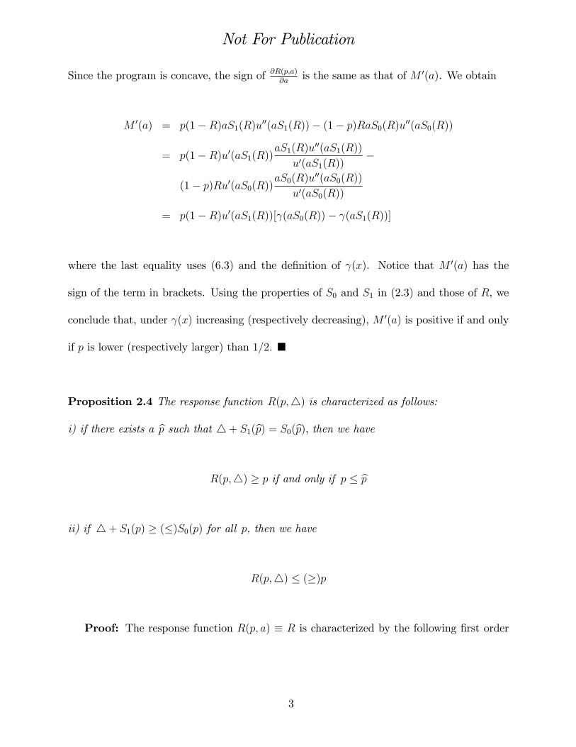
Not For Publication

Since the program is concave, the sign of @R(p;a)@a

is the same as that of M 0(a). We obtain

M 0(a) = p(1�R)aS1(R)u00(aS1(R))� (1� p)RaS0(R)u00(aS0(R))

= p(1�R)u0(aS1(R))aS1(R)u

00(aS1(R))

u0(aS1(R))�

(1� p)Ru0(aS0(R))aS0(R)u

00(aS0(R))

u0(aS0(R))

= p(1�R)u0(aS1(R))[ (aS0(R))� (aS1(R))]

where the last equality uses (6.3) and the de�nition of (x). Notice that M 0(a) has the

sign of the term in brackets. Using the properties of S0 and S1 in (2.3) and those of R, we

conclude that, under (x) increasing (respectively decreasing), M 0(a) is positive if and only

if p is lower (respectively larger) than 1=2. �

Proposition 2.4 The response function R(p;4) is characterized as follows:

i) if there exists a bp such that 4+ S1(bp) = S0(bp), then we haveR(p;4) � p if and only if p � bp

ii) if 4+ S1(p) � (�)S0(p) for all p, then we have

R(p;4) � (�)p

Proof: The response function R(p; a) � R is characterized by the following �rst order

53

Not For Publication

condition

g(4; R) � p(1�R)u0(4+ S1(R))� (1� p)Ru0(S0(R)) = 0

We compute the marginal bene�t of increasing R at p :

g(4; p) = p(1� p)[u0(4+ S1(p))� u0(S0(p))]

which is positive if and only if

N(p) � 4+ S1(p)� S0(p) � 0

We thus have R � p if and only if N(p) � 0. Since, by our assumptions on the PSR, N(p)

is strictly increasing, there is at most one bp satisfying N(bp) = 0. Therefore either bp existsand we are in case i), or bp does not exist and we are in case ii). It is then direct to concludethe proof for each case i) and ii).�

Proposition 2.5 The solutions R(p) and �(p) to program (2.9) satisfy the following prop-

erties:

i) for p � p(k), we have �(p) = 0 and R(p) 2 [0; 11+k] with R0(p) > 0,

ii) for p in [p(k); p(k)], we have �(p) 2 [0; �] with �0(p) > 0 and R(p) = 11+k,

iii) for p � p(k), we have �(p) = � and R(p) 2 [ 11+k; 1] with R0(p) > 0,

54

Not For Publication

together with

p(k) =u0(S0(

11+k) + �)

ku0(S1(11+k) + �) + u0(S0(

11+k) + �)

and

p(k) =u0(S0(

11+k) + (k + 1)�)

ku0(S1(11+k) + (k + 1)�) + u0(S0(

11+k))

Proof : The conditions which characterize the interior solutions (��, q�) of the program

(2.9) are

pku0(S1(q�) + k�� + �)� (1� p)u0(S0(q�)� �� + �) = 0 (6.4)

p(1� q�)u0(S1(q�) + k�� + �)� (1� p)q�u0(S0(q�)� �� + �) = 0 (6.5)

which imply q� = 11+k.

Therefore the condition (6.4) writes

pku0(S1(1

1 + k) + k�� + �)� (1� p)u0(S0(

1

1 + k)� �� + �) = 0 (6.6)

Di¤erentiating with respect to p and rearranging yields

@��

@p= �

ku0(S1(11+k) + k�� + �) + u0(S0(

11+k)� �� + �)

pk2u00(S1(11+k) + k�� + �) + (1� p)u00(S0( 1

1+k)� �� + �)

> 0

Therefore �� can only increase in p; moreover, the condition (6.4) cannot be satis�ed at

p = 0 or at p = 1. Indeed it is strictly negative at p = 0 and strictly positive at p = 1.

Consequently, �(p) is �rst equal to zero, then equal to �� > 0 and strictly increasing in p, and

�nally constant and equal to �. There are thus two critical values of subjective probability

55

Not For Publication

denoted p(k) and p(k) with 0 < p(k) < p(k) < 1 such that the optimal � is equal to zero for

p � p(k) and is equal to � for p � p(k). Moreover, the response function R(p) = 11+k

when

p is in [p(k); p(k)].

We now study more speci�cally the response function when p � p(k). Since �� = 0,

the response function R(p) is equal to the reported probability without hedging e¤ects, as

characterized by q solving

p(1� q)u0(S1(q) + �)� (1� p)qu0(S0(q) + �) = 0

The threshold probability p(k) is de�ned by the p solving

pku0(S1(1

1 + k) + �)� (1� p)u0(S0(

1

1 + k) + �) = 0

We thus have

p(k) =u0(S0(

11+k) + �)

ku0(S1(11+k) + �) + u0(S0(

11+k) + �)

as stated in the Proposition. Moreover, this implies p(k) < 11+k

if and only if k > 1. Notice

also that an increase in k decreases p(k). Finally, it is easy to check that R(p(k)) = 11+k.

We �nally study the response function when p � p(k). Since �� = �, the optimal

reported probability q is de�ned by

p(1� q)u0(S1(q) + (k + 1)�)� (1� p)qu0(S0(q)) = 0

56

Not For Publication

The threshold probability p(k) is de�ned by the p solving

pku0(S1(1

1 + k) + (k + 1)�)� (1� p)u0(S0(

1

1 + k)) = 0;

that is by

p(k) =u0(S0(

11+k))

ku0(S1(11+k) + (k + 1)�) + u0(S0(

11+k))

as stated in the Proposition.�

57

Not For Publication

Appendix B: The E¤ect of Ambiguity Aversion

We consider the theory of ambiguity introduced by KMM (2005). We assume that the

agent�s subjective probabilities are represented by a random variable ep, to which the possiblerealizations belong to [0; 1]. Consistent with KMM preferences, an ambiguity averse agent

facing a PSR solves

maxq(E�(epu(S1(q)) + (1� ep)u(S0(q))))

in which � is assumed to be continuously di¤erentiable, strictly increasing, and concave.

Under KMM preferences, the concavity of � corresponds to ambiguity aversion. The �rst

order condition is

K(q) � Ef(ep(1� q)u0(S1(q))� (1� ep)qu(S0(q)))�0(epu(S1(q)) + (1� ep)u(S0(q)))g = 0 (6.7)It can be easily checked that the second order condition is satis�ed under u and � concave.

Our objective is to compare the response function of an ambiguity averse agent to that of

an ambiguity neutral agent. Under � linear, the agent is ambiguity neutral and essentially

behaves as an expected utility maximizer, reporting q� de�ned by

E(ep(1� q�)u0(S1(q�))� (1� ep)q�u(S0(q�))) = 0Observe that this last condition is equivalent to (2.5) with p = Eep. We are done if we cancompute the sign of K(q�), which expresses the marginal bene�t under ambiguity aversion

of increasing q at the optimal reported probability q� under ambiguity neutrality. Denoting

61

Not For Publication

as before f(p; q) � p(1� q)u0(S1(q))� (1� p)qu0(S0(q)) and using the previous equality, we

have

K(q�) = Covep[f(ep; q�); �0(epu(S1(q�)) + (1� ep)u(S0(q�)))]We now use the following Lemma stating the well-known covariance rule (e.g., Kimball 1951).

Lemma B.1 If X(p) is increasing in p; then Covep(X(ep); Y (ep)) � 0 if and only if Y (p) isdecreasing in p.

Observe that f(p; q) is increasing in p. Moreover, observe that the derivative of �0(pu(S1(q�))+

(1 � p)u(S0(q�))) with respect to p has the sign of S0(q�) � S1(q�) under �00 < 0. Conse-

quently, K(q�) is positive if and only if q� is lower than 1=2. We then use Corollary 2.1 that

characterizes q� and the properties of the PSR in (2.3) to obtain the next Proposition. In

this Proposition, we denote Ra(ep) the optimal reported probability under ambiguity aversion(� concave) and R(ep) the optimal reported probability under expected utility (� linear) witha subjective probability Eep.

Proposition B.1 Ra(ep) � R(ep) if and only if Eep � 1=2.

Essentially, this result indicates that ambiguity aversion leads to reporting more uni-

form probabilities compared to ambiguity neutrality (i.e., expected utility). In other words,

ambiguity aversion reinforces the bias induced by risk aversion. It is also possible to show

that ambiguity aversion reinforces the e¤ect of risk aversion when there is a stake. That is,

62

Not For Publication

ambiguity aversion leads to increasing the response function before the �xed point and to

decreasing the response function after the �xed point.

A particular case is u(x) = x. In that case, the agent is ambiguity averse but risk neutral.

This implies q� = Eep: when the agent is both ambiguity neutral and risk neutral, she alwaysreports the mean of her subjective beliefs Eep by the de�nition of a PSR. Proposition B.1then reduces to the following Corollary.

Corollary B.1 Ra(ep) � Eep if and only if Eep � 1=2.

This Corollary, similar to Corollary 2.1, thus further suggests that the e¤ect of ambiguity

aversion is similar to that of risk aversion.

63

Not For Publication Appendix C Identification Code :______

INSTRUCTIONS

(translated from French)

You are about to take part in an experiment aimed at better understanding decisions made under uncertainty. In the

experiment you will earn an amount of money. This amount of money will be paid to you at the end of the experiment,

outside the lab, in private, and in cash. The amount of money you will earn may be larger if :

1. You read the instructions below carefully.

2. You follow these instructions precisely.

3. You make thoughtful decisions during the experiment.

If you have any questions while we read the instructions or during the experiment, then call us by raising your hand.

Any form of communication between participants is absolutely forbidden. If you do not follow this rule, then we will

have to exclude you from the experiment without any payment.

The Task You will be given 30 different «events», divided into 3 series of 10. Each of these events describes the possible

outcome produced by the roll of 2 dice. One of the die is red, the other die is black. Each die has 10 sides numbered

from 0 to 9. Each die is fair, which means that any of the 10 sides has an equal chance to come up when the die is

rolled. Consider now two examples of events we could give you:

Event 1: «The red die equals 5 and the black die equals 3».

Event 2: «The red die produces a number strictly greater than the black die».

As explained below, 1 out of the 30 events will be randomly selected for payment at the end of the experiment. We

will then roll the 2 dice once in order to determine whether the event occurs or whether the event does not occur. For

instance, if Event 1 above is randomly selected for payment, then we will say that Event 1 occurred when the outcome

of the roll of the 2 die is such that the red die produces a 5 and the black die produces a 3. For any other number

produced by either the black or the red die, we will say that Event 1 did not occur. Likewise, if Event 2 is randomly

selected for payment, then we will say that Event 2 occurred when the outcome of the roll of the 2 dice is such that the

red die produces a number strictly greater than the black die. Otherwise, we will say that Event 2 did not occur.

Your Choices: For each of the 30 events, you will be asked to make a choice. One of these choices will determine the amount of

money you will earn both when the event randomly selected for payment occurs and when it does not occur. Each of

your choices consists in selecting a number between 1 and 149 in the table we gave you separately. We will now

explain how your choice for the event randomly selected for payment affects the amount of money you will earn.

If you look at the table, you can see that there are two amounts associated with each of the 149 possible choice

numbers. The first is the amount of money you receive if the event occurs. The second is the amount of money you

Not For Publication receive if the event does not occur. For instance, you can see in the table that the amounts associated with the choice

number “1” are 53 and 4,000. This means that the amount of money you earn would be 53FCFA if the event occurs or

4,000FCFA if the event does not occur. As you can see, when the choice number increases from 1 to 149, the amounts

in the first columns increase, while the amounts in the second column decrease. For instance, the amounts associated

with the choice number “90” are 3,360FCA and 2,560FCFA. In other words, if you choose the number “90” instead of

the number “1” then you would earn more if the event occurs (3,360FCFA instead of 53FCFA), but you would earn

less if the event does not occur (2,560FCFA instead of 4,000FCFA). Note also, that the highest choice numbers (those

closer to 149) produce the largest amounts of money when the event occurs, but the smallest amounts of money when

the event does not occur. For instance, the choice number “140” produces 3,982FCFA if the event occurs, but only

516FCFA when the event does not occur.

For each of the 30 events, you are free to select any choice number you want. Note that there is no correct or incorrect

choice. The choice numbers selected may differ from one individual to the next. In general however, you may find it

profitable to choose a higher choice number when you think the chances that the event occurs are higher. Indeed, as

we just explained, such a choice number will produce a larger amount if the event occurs. Conversely, you may find it

profitable to choose a smaller number when you think the chances that the event occurs are lower.

Your Payment The amount of money you receive today will be determined in 3 steps. In a first step, we will randomly select one of

the 30 events for payment. In a second step, we will roll the 2 dice once to determine whether the event selected for

payment occurs or does not occur. Finally, in a third step, we will look at the choice number you chose for the event

selected for payment in order to determine the amount of money you will receive.

We will proceed as follows to select one of the 30 events for payment. At the beginning of the experiment, we will ask

you to write your identification code on a piece of paper that you will then fold. Your identification code is located on

the top right hand corner on the first page of the instructions. At the end of the experiment, we will draw at random

one of the pieces of paper. The person whose identification number has been drawn will randomly choose 1 out of 30

numbered tokens from a bag. The number written on the token selected indicates the event that will be considered for

the payment of each person in the room.

We will then draw at random a second piece of paper. The person whose identification code has been drawn will roll

the 2 dice once to determine whether the event selected occurs or not. This single roll will be used to determine the

payment of each person in the room.

If you do not wish to be one of the persons rolling the dice or drawing the token, then simply leave your piece of paper

blank. Just fold it without writing your identification code.

Not For Publication Comprehension Test: Understanding the instructions well is important if you want to improve your chances to earn a larger amount of

money during the experiment. In order to make sure you understand the instructions well, we will now conduct a

quick test without monetary consequences. Imagine first that Event 1: «The red die equals 5 and the black die equals

3» has been selected for payment. In addition, imagine that an individual selected the choice number 98 for this event,

while a different individual selected the choice number 139. Please, write in the table below the amount of money

each of these 2 individuals would receive if the roll of the dice produces the following outcomes:

Outcome produced by the roll of the 2 dice Payment to the individual with

A choice number of 98 A choice number of 139

The red die equals 6 and the black die equals 4 ________FCFA ________FCFA

The red die equals 5 and the black die equals 4 ________FCFA ________FCFA

The red die equals 5 and the black die equals 3 ________FCFA ________FCFA

Imagine now that Event 2: «The red die produces a number strictly greater than the black die» has been selected for

payment. In addition, imagine that an individual selected the choice number 6 for this event, while a different

individual selected the choice number 71. Please, write in the table below the amount of money each of these 2

individuals would receive if the roll of the dice produce the following outcomes:

Outcome produced by the roll of the 2 dice Payment to the individual with

A choice number of 6 A choice number of 71

The red die equals 3 and the black die equals 9 ________FCFA ________FCFA

The red die equals 5 and the black die equals 2 ________FCFA ________FCFA

The red die equals 0 and the black die equals 5 ________FCFA ________FCFA

Please, do not hesitate to raise your hand now if the instructions we just read were not perfectly clear. Once the

experiment starts you can still call us to answer any question by raising your hand.

Note that the amount of money you will receive today may be larger or smaller depending on your choices and on the

outcome produced by the roll of the 2 dice. By accepting to participate in the experiment, you accept the

consequences associated with your choices and with the roll of the dice. If you do not wish to participate in the

experiment you are free to leave now, in which case you will receive a flat fee of 500FCFA.

Not For Publication

Series 1 : For the first series of 10 events, we will consider that the red die determines the first digit (meaning 0, 10, 20, 30, 40,

50, 60, 70, 80, or 90) and the black die determines the second digit (meaning 0, 1, 2, 3, 4, 5, 6, 7, 8, or 9) of a number

between 1 and 100 (both dice equal to zero corresponds to the number 100). As a result, every number between 1 and

100 has an equal chance to come out from the roll of the 2 dice.

Event

Description

Your Choice Number

1 « the number is between 1 (included) and 25 (included) »

2 « the number is between 62 (included) and 66 (included) »

3 « the number is between 16 (included) and 76 (included) »

4 « the number is between 3 (included) and 92 (included) »

5 « the number is between 52 (included) and 96 (included) »

6 « the number is between 9 (included) and 88 (included) »

7 « the number is between 44 (included) and 58 (included) »

8 « the number is between 23 (included) and 25 (included) »

9 « the number is between 37 (included) and 71 (included) »

10 « the number is between 28 (included) and 97 (included) »

Series 2 : For the next series of 10 events, we will sum the outcome of the red die to the outcome of the black die. Since each die

can only produce a number between 0 and 9, the sum obtained can only be a number between 0 and 18. Observe that

some of these sums (for instance 0) can only be obtained from a unique combination of the 2 dice, while other sums

(for instance 6) can be obtained from multiple combinations of the 2 dice. As a result, some of the 19 possible sums

have more chances to come out than other sums.

Event

Description

Your Choice Number

11 « The sum is between 0 (included) and 4 (included) »

12 « The sum is between 2 (included) and 10 (included) »

13 « The sum is equal to 16 »

14 « The sum is between 4 (included) and 14 (included) »

15 « The sum is between 5 (included) and 13 (included) »

16 « The sum is between 0 (included) and 14 (included) »

17 « The sum is between 10 (included) and 18 (included) »

18 « The sum is equal to 4 »

19 « The sum is between 11 (included) and 17 (included) »

20 « The sum is between 2 (included) and 6 (included) »

Not For Publication Series 3 : The last series of 10 events is similar to the first series. The red die determines the first digit and the black die

determines the second digit of a number between 1 and 100. The difference with the first series is that, when you

select your choice number, you are not facing 1, but 2 possible events. For instance, the 1st of the 2 possible events

could be «the number is between 1 (included) and 25 (included)» and the 2nd of the 2 possible events could be «the

number is between 55 (included) and 59 (included)». You are asked to select a single choice number without

knowing which of the 2 possible events will be used to determine your payment. It is only at the end of the experiment

that we will toss a coin to identify which of the 2 possible events will be used for payment. If the coin lands on Heads,

then your payment will be determined using the 1st event. If the coin lands on Tails, then your payment will be

determined using the 2nd event. As with Series 1, we will then roll the 2 dice to determine whether the event identified

by the coin toss occurs or not. Here is an example :

♦ If the coin lands on Heads, then the event is :

«the number is between 1 (included) and 25 (included)».

♦ Or, if the coin lands on Tails, then the event is :

«the number is between 55 (included) and 59 (included)».

You must select a unique choice number before you know which of the possible 2 events will be used for payment.

Imagine for instance that an individual selects the choice number 70. We have to distinguish between different 2

situations to determine how much the individual will be paid:

♦ Either the coin tossed at the end of the experiment lands on Heads. In this case, the event used for payment

is «the number is between 1 (included) and 25 (included)». Then, the event occurs if the 2 dice produce a

number that is indeed between 1 (included) and 25 (included), and the individual in our example is paid

2,862FCFA. On the other hand, if the 2 dice produce a number that is not between 1 (included) and 25

(included), then the event does not occur and the individual in our example is paid 3,129FCFA.

♦ Or the coin tossed at the end of the experiment lands on Tails. In this case, the event identified is «the

number is between 55 (included) and 59 (included)». Then, the event occurs if the 2 dice produce a number

that is indeed between 55 (included) and 59 (included), and the individual in our example is paid 2,862FCFA.

On the other hand, if the 2 dice produce a number that is between 55 (included) and 59 (included), then the

event does not occur and the individual in our example is paid 3,129FCFA.

To summarize, there are only 2 cases under which the event occurs : 1) The coin lands on Heads and the 2 dice

produce a number between 1 (included) and 25 (included), or 2) the coin lands on Tails and the 2 dice produce a

number between 55 (included) and 59 (included). In all other cases, the event does not occur. Thus, when you select

your choice number, you might want to imagine the different cases under which the event occurs and does not occur.

If these explanations are not sufficiently clear, please call us by raising your hand. We will then come to your desk to

answer any questions you may have. We would like to remind you that it is important for you to understand the

instructions well so that you can make the decisions that suit you the best.

Not For Publication

Event

Description

Your Choice Number

21

♦ If the coin lands on Heads, then the event is :

«the number is between 48 (included) and 82 (included)».

♦ Or, if the coin lands on Tails, then the event is :

«the number is between 14 (included) and 48 (included)».

22

♦ If the coin lands on Heads, then the event is :

«the number is between 21 (included) and 35 (included)».

♦ Or, if the coin lands on Tails, then the event is :

«the number is between 30 (included) and 44 (included)».

23

♦ If the coin lands on Heads, then the event is :

«the number is between 25 (included) and 89 (included)».

♦ Or, if the coin lands on Tails, then the event is :

«the number is between 2 (included) and 96 (included)».

24

♦ If the coin lands on Heads, then the event is :

«the number is between 66 (included) and 97 (included)».

♦ Or, if the coin lands on Tails, then the event is :

«the number is between 13 (included) and 70 (included)».

25

♦ If the coin lands on Heads, then the event is :

«the number is between 56 (included) and 58 (included)».

♦ Or, if the coin lands on Tails, then the event is :

«the number is between 78 (included) and 80 (included)».

26

♦ If the coin lands on Heads, then the event is :

«the number is between 82 (included) and 89 (included)».

♦ Or, if the coin lands on Tails, then the event is :

«the number is between 25 (included) and 66 (included)».

27

♦ If the coin lands on Heads, then the event is :

«the number is between 7 (included) and 88 (included)».

♦ Or, if the coin lands on Tails, then the event is :

«the number is between 3 (included) and 100 (included)».

28

♦ If the coin lands on Heads, then the event is :

«the number is equal to 12».

♦ Or, if the coin lands on Tails, then the event is :

«the number is between 49 (included) and 57 (included)».

29

♦ If the coin lands on Heads, then the event is :

«the number is between 26 (included) and 86 (included)».

♦ Or, if the coin lands on Tails, then the event is :

«the number is between 14 (included) and 74 (included)».

30

♦ If the coin lands on Heads, then the event is :

«the number is between 1 (included) and 83 (included)».

♦ Or, if the coin lands on Tails, then the event is :

«the number is between 36 (included) and 91 (included)».

Not For Publication

Choice Number 

Your Payment (in FCFA) when the Event

Choice Number 

 

Your Payment (in FCFA) when the Event

Choice Number 

Your Payment (in FCFA) when the Event

Occurs Does not Occur Occurs Does not

Occur Occurs Does not Occur

1 53 4000 51 2258 3538 101 3573 2186 2 106 3999 52 2293 3519 102 3590 2150 3 158 3998 53 2327 3501 103 3607 2114 4 210 3997 54 2362 3482 104 3624 2077 5 262 3996 55 2396 3462 105 3640 2040 6 314 3994 56 2429 3442 106 3656 2002 7 365 3991 57 2462 3422 107 3671 1965 8 415 3989 58 2495 3402 108 3686 1926 9 466 3986 59 2528 3381 109 3701 1888 10 516 3982 60 2560 3360 110 3716 1849 11 565 3978 61 2592 3338 111 3730 1810 12 614 3974 62 2623 3317 112 3743 1770 13 663 3970 63 2654 3294 113 3757 1730 14 712 3965 64 2685 3272 114 3770 1690 15 760 3960 65 2716 3249 115 3782 1649 16 808 3954 66 2746 3226 116 3794 1608 17 855 3949 67 2775 3202 117 3806 1566 18 902 3942 68 2805 3178 118 3818 1525 19 949 3936 69 2834 3154 119 3829 1482 20 996 3929 70 2862 3129 120 3840 1440 21 1042 3922 71 2890 3104 121 3850 1397 22 1087 3914 72 2918 3078 122 3861 1354 23 1133 3906 73 2946 3053 123 3870 1310 24 1178 3898 74 2973 3026 124 3880 1266 25 1222 3889 75 3000 3000 125 3889 1222 26 1266 3880 76 3026 2973 126 3898 1178 27 1310 3870 77 3053 2946 127 3906 1133 28 1354 3861 78 3078 2918 128 3914 1087 29 1397 3850 79 3104 2890 129 3922 1042 30 1440 3840 80 3129 2862 130 3929 996 31 1482 3829 81 3154 2834 131 3936 949 32 1525 3818 82 3178 2805 132 3942 902 33 1566 3806 83 3202 2775 133 3949 855 34 1608 3794 84 3226 2746 134 3954 808 35 1649 3782 85 3249 2716 135 3960 760 36 1690 3770 86 3272 2685 136 3965 712 37 1730 3757 87 3294 2654 137 3970 663 38 1770 3743 88 3317 2623 138 3974 614 39 1810 3730 89 3338 2592 139 3978 565 40 1849 3716 90 3360 2560 140 3982 516 41 1888 3701 91 3381 2528 141 3986 466 42 1926 3686 92 3402 2495 142 3989 415 43 1965 3671 93 3422 2462 143 3991 365 44 2002 3656 94 3442 2429 144 3994 314 45 2040 3640 95 3462 2396 145 3996 262 46 2077 3624 96 3482 2362 146 3997 210 47 2114 3607 97 3501 2327 147 3998 158 48 2150 3590 98 3519 2293 148 3999 106 49 2186 3573 99 3538 2258 149 4000 53 50 2222 3556 100 3556 2222