Elias M. Stein and Rami Shakarchi: Complex Analysisassets.press.princeton.edu/chapters/s02_7563.pdf · Elias M. Stein and Rami Shakarchi: Complex Analysis . 2 Cauchy’s Theorem and

COPYRIGHT NOTICE:

For COURSE PACK and other PERMISSIONS, refer to entry on previous page. Formore information, send e-mail to [email protected]

University Press. All rights reserved. No part of this book may be reproduced in any formby any electronic or mechanical means (including photocopying, recording, or information storage and retrieval) without permission in writing from the publisher, except for reading and browsing via the World Wide Web. Users are not permitted to mount this file on any network servers.

is published by Princeton University Press and copyrighted, © 2003, by Princeton

Elias M. Stein and Rami Shakarchi: Complex Analysis

2 Cauchy’s Theorem and ItsApplications

The solution of a large number of problems can bereduced, in the last analysis, to the evaluation of def-inite integrals; thus mathematicians have been muchoccupied with this task... However, among many re-sults obtained, a number were initially discovered bythe aid of a type of induction based on the passagefrom real to imaginary. Often passage of this kindled directly to remarkable results. Nevertheless thispart of the theory, as has been observed by Laplace,is subject to various difficulties...

After having reflected on this subject and broughttogether various results mentioned above, I hope toestablish the passage from the real to the imaginarybased on a direct and rigorous analysis; my researcheshave thus led me to the method which is the object ofthis memoir...

A. L. Cauchy, 1827

In the previous chapter, we discussed several preliminary ideas in com-plex analysis: open sets in C, holomorphic functions, and integrationalong curves. The first remarkable result of the theory exhibits a deepconnection between these notions. Loosely stated, Cauchy’s theoremsays that if f is holomorphic in an open set Ω and γ ⊂ Ω is a closedcurve whose interior is also contained in Ω then

(1)

∫

γ

f(z) dz = 0.

Many results that follow, and in particular the calculus of residues, arerelated in one way or another to this fact.

A precise and general formulation of Cauchy’s theorem requires defin-ing unambiguously the “interior” of a curve, and this is not always aneasy task. At this early stage of our study, we shall make use of thedevice of limiting ourselves to regions whose boundaries are curves thatare “toy contours.” As the name suggests, these are closed curves whosevisualization is so simple that the notion of their interior will be unam-

33

biguous, and the proof of Cauchy’s theorem in this setting will be quitedirect. For many applications, it will suffice to restrict ourselves to thesetypes of curves. At a later stage, we take up the questions related tomore general curves, their interiors, and the extended form of Cauchy’stheorem.

Our initial version of Cauchy’s theorem begins with the observationthat it suffices that f have a primitive in Ω, by Corollary 3.3 in Chapter 1.The existence of such a primitive for toy contours will follow from atheorem of Goursat (which is itself a simple special case)1 that assertsthat if f is holomorphic in an open set that contains a triangle T and itsinterior, then ∫

T

f(z) dz = 0.

It is noteworthy that this simple case of Cauchy’s theorem suffices toprove some of its more complicated versions. From there, we can provethe existence of primitives in the interior of some simple regions, andtherefore prove Cauchy’s theorem in that setting. As a first applicationof this viewpoint, we evaluate several real integrals by using appropriatetoy contours.

The above ideas also lead us to a central result of this chapter, theCauchy integral formula; this states that if f is holomorphic in an openset containing a circle C and its interior, then for all z inside C,

f(z) =1

2πi

∫

C

f(ζ)

ζ − zdζ.

Differentiation of this identity yields other integral formulas, and inparticular we obtain the regularity of holomorphic functions. This isremarkable, since holomorphicity assumed only the existence of the firstderivative, and yet we obtain as a consequence the existence of derivativesof all orders. (An analogous statement is decisively false in the case ofreal variables!)

The theory developed up to that point already has a number of note-worthy consequences:

• The property at the base of “analytic continuation,” namely that aholomorphic function is determined by its restriction to any opensubset of its domain of definition. This is a consequence of the factthat holomorphic functions have power series expansions.

1Goursat’s result came after Cauchy’s theorem, and its interest is the technical factthat its proof requires only the existence of the complex derivative at each point, and notits continuity. For the earlier proof, see Exercise 5.

34 Chapter 2. CAUCHY’S THEOREM AND ITS APPLICATIONS

• Liouville’s theorem, which yields a quick proof of the fundamentaltheorem of algebra.

• Morera’s theorem, which gives a simple integral characterizationof holomorphic functions, and shows that these functions are pre-served under uniform limits.

1 Goursat’s theorem

Corollary 3.3 in the previous chapter says that if f has a primitive in anopen set Ω, then ∫

γ

f(z) dz = 0

for any closed curve γ in Ω. Conversely, if we can show that the aboverelation holds for some types of curves γ, then a primitive will exist. Ourstarting point is Goursat’s theorem, from which in effect we shall deducemost of the other results in this chapter.

Theorem 1.1 If Ω is an open set in C, and T ⊂ Ω a triangle whoseinterior is also contained in Ω, then

∫

T

f(z) dz = 0

whenever f is holomorphic in Ω.

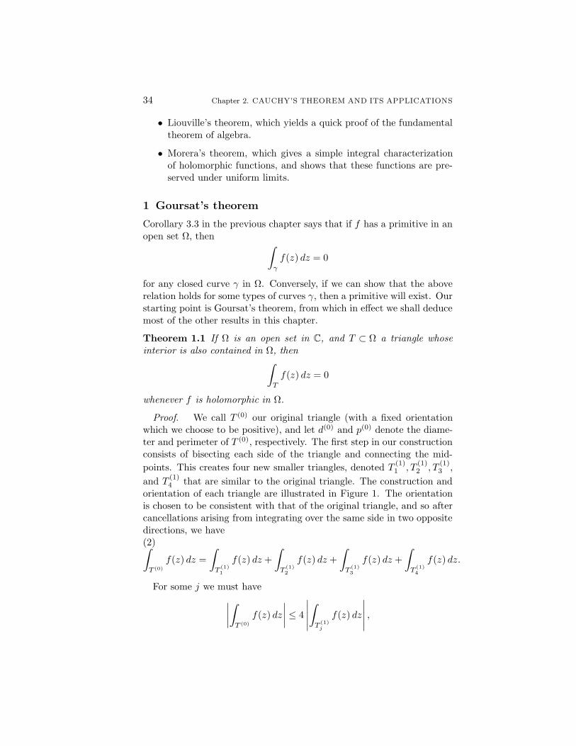
Proof. We call T (0) our original triangle (with a fixed orientationwhich we choose to be positive), and let d(0) and p(0) denote the diame-ter and perimeter of T (0), respectively. The first step in our constructionconsists of bisecting each side of the triangle and connecting the mid-

points. This creates four new smaller triangles, denoted T(1)1 , T

(1)2 , T

(1)3 ,

and T(1)4 that are similar to the original triangle. The construction and

orientation of each triangle are illustrated in Figure 1. The orientationis chosen to be consistent with that of the original triangle, and so aftercancellations arising from integrating over the same side in two oppositedirections, we have(2)∫

T (0)

f(z) dz =

∫

T(1)1

f(z) dz +

∫

T(1)2

f(z) dz +

∫

T(1)3

f(z) dz +

∫

T(1)4

f(z) dz.

For some j we must have

∣∣∣∣∫

T (0)

f(z) dz

∣∣∣∣ ≤ 4

∣∣∣∣∣

∫

T(1)j

f(z) dz

∣∣∣∣∣ ,

1. Goursat’s theorem 35

T(1)2

T(1)1

T(1)3

T(1)4

T (0)

Figure 1. Bisection of T (0)

for otherwise (2) would be contradicted. We choose a triangle thatsatisfies this inequality, and rename it T (1). Observe that if d(1) andp(1) denote the diameter and perimeter of T (1), respectively, then d(1) =(1/2)d(0) and p(1) = (1/2)p(0). We now repeat this process for the trian-gle T (1), bisecting it into four smaller triangles. Continuing this process,we obtain a sequence of triangles

T (0), T (1), . . . , T (n), . . .

with the properties that∣∣∣∣∫

T (0)

f(z) dz

∣∣∣∣ ≤ 4n

∣∣∣∣∫

T (n)

f(z) dz

∣∣∣∣

and

d(n) = 2−nd(0), p(n) = 2−np(0)

where d(n) and p(n) denote the diameter and perimeter of T (n), respec-tively. We also denote by T (n) the solid closed triangle with boundaryT (n), and observe that our construction yields a sequence of nested com-pact sets

T (0) ⊃ T (1) ⊃ · · · ⊃ T (n) ⊃ · · ·

whose diameter goes to 0. By Proposition 1.4 in Chapter 1, there existsa unique point z0 that belongs to all the solid triangles T (n). Since f isholomorphic at z0 we can write

f(z) = f(z0) + f ′(z0)(z − z0) + ψ(z)(z − z0) ,

where ψ(z) → 0 as z → z0. Since the constant f(z0) and the linear func-tion f ′(z0)(z − z0) have primitives, we can integrate the above equalityusing Corollary 3.3 in the previous chapter, and obtain

(3)

∫

T (n)

f(z) dz =

∫

T (n)

ψ(z)(z − z0) dz.


Now z0 belongs to the closure of the solid triangle T (n) and z to itsboundary, so we must have |z − z0| ≤ d(n), and using (3) we get, by (iii)in Proposition 3.1 of the previous chapter, the estimate

∣∣∣∣∫

T (n)

f(z) dz

∣∣∣∣ ≤ εnd(n)p(n),

where εn = supz∈T (n) |ψ(z)| → 0 as n→ ∞. Therefore

∣∣∣∣∫

T (n)

f(z) dz

∣∣∣∣ ≤ εn4−nd(0)p(0) ,

which yields our final estimate

∣∣∣∣∫

T (0)

f(z) dz

∣∣∣∣ ≤ 4n

∣∣∣∣∫

T (n)

f(z) dz

∣∣∣∣ ≤ εnd(0)p(0).

Letting n→ ∞ concludes the proof since εn → 0.

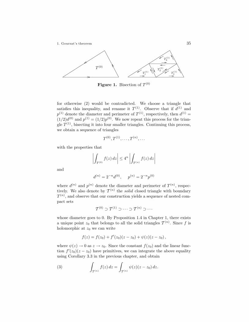
Corollary 1.2 If f is holomorphic in an open set Ω that contains arectangle R and its interior, then

∫

R

f(z) dz = 0.

This is immediate since we first choose an orientation as in Figure 2and note that

∫

R

f(z) dz =

∫

T1

f(z) dz +

∫

T2

f(z) dz.

T2

T1

R

Figure 2. A rectangle as the union of two triangles

2. Local existence of primitives and Cauchy’s theorem in a disc 37

2 Local existence of primitives and Cauchy’s theorem in

a disc

We first prove the existence of primitives in a disc as a consequence ofGoursat’s theorem.

Theorem 2.1 A holomorphic function in an open disc has a primitivein that disc.

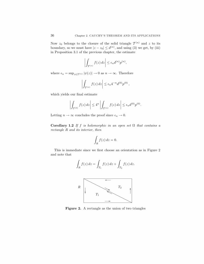
Proof. After a translation, we may assume without loss of generalitythat the disc, say D, is centered at the origin. Given a point z ∈ D,consider the piecewise-smooth curve that joins 0 to z first by moving inthe horizontal direction from 0 to z where z = Re(z), and then in thevertical direction from z to z. We choose the orientation from 0 to z,and denote this polygonal line (which consists of at most two segments)by γz , as shown on Figure 3.

γz

0 z

z

Figure 3. The polygonal line γz

Define

F (z) =

∫

γz

f(w) dw.

The choice of γz gives an unambiguous definition of the function F (z).We contend that F is holomorphic in D and F ′(z) = f(z). To prove this,fix z ∈ D and let h ∈ C be so small that z + h also belongs to the disc.Now consider the difference

F (z + h) − F (z) =

∫

γz+h

f(w) dw −∫

γz

f(w) dw.


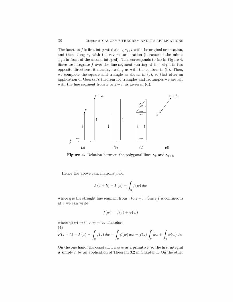
The function f is first integrated along γz+h with the original orientation,and then along γz with the reverse orientation (because of the minussign in front of the second integral). This corresponds to (a) in Figure 4.Since we integrate f over the line segment starting at the origin in twoopposite directions, it cancels, leaving us with the contour in (b). Then,we complete the square and triangle as shown in (c), so that after anapplication of Goursat’s theorem for triangles and rectangles we are leftwith the line segment from z to z + h as given in (d).

(a) (b) (c) (d)

0

z + h

z

z + h

z

Figure 4. Relation between the polygonal lines γz and γz+h

Hence the above cancellations yield

F (z + h) − F (z) =

∫

η

f(w) dw

where η is the straight line segment from z to z + h. Since f is continuousat z we can write

f(w) = f(z) + ψ(w)

where ψ(w) → 0 as w → z. Therefore(4)

F (z + h) − F (z) =

∫

η

f(z) dw +

∫

η

ψ(w) dw = f(z)

∫

η

dw +

∫

η

ψ(w) dw.

On the one hand, the constant 1 has w as a primitive, so the first integralis simply h by an application of Theorem 3.2 in Chapter 1. On the other

2. Local existence of primitives and Cauchy’s theorem in a disc 39

hand, we have the following estimate:

∣∣∣∣∫

η

ψ(w) dw

∣∣∣∣ ≤ supw∈η

|ψ(w)| |h|.

Since the supremum above goes to 0 as h tends to 0, we conclude fromequation (4) that

limh→0

F (z + h) − F (z)

h= f(z) ,

thereby proving that F is a primitive for f on the disc.

This theorem says that locally, every holomorphic function has a prim-itive. It is crucial to realize, however, that the theorem is true not onlyfor arbitrary discs, but also for other sets as well. We shall return to thispoint shortly in our discussion of “toy contours.”

Theorem 2.2 (Cauchy’s theorem for a disc) If f is holomorphic ina disc, then

∫

γ

f(z) dz = 0

for any closed curve γ in that disc.

Proof. Since f has a primitive, we can apply Corollary 3.3 of Chap-ter 1.

Corollary 2.3 Suppose f is holomorphic in an open set containing thecircle C and its interior. Then

∫

C

f(z) dz = 0.

Proof. Let D be the disc with boundary circle C. Then there existsa slightly larger disc D′ which contains D and so that f is holomorphicon D′. We may now apply Cauchy’s theorem in D′ to conclude that∫

Cf(z) dz = 0.

In fact, the proofs of the theorem and its corollary apply whenever wecan define without ambiguity the “interior” of a contour, and constructappropriate polygonal paths in an open neighborhood of that contourand its interior. In the case of the circle, whose interior is the disc, therewas no problem since the geometry of the disc made it simple to travelhorizontally and vertically inside it.


The following definition is loosely stated, although its applicationswill be clear and unambiguous. We call a toy contour any closed curvewhere the notion of interior is obvious, and a construction similar tothat in Theorem 2.1 is possible in a neighborhood of the curve and itsinterior. Its positive orientation is that for which the interior is to the leftas we travel along the toy contour. This is consistent with the definitionof the positive orientation of a circle. For example, circles, triangles,and rectangles are toy contours, since in each case we can modify (andactually copy) the argument given previously.

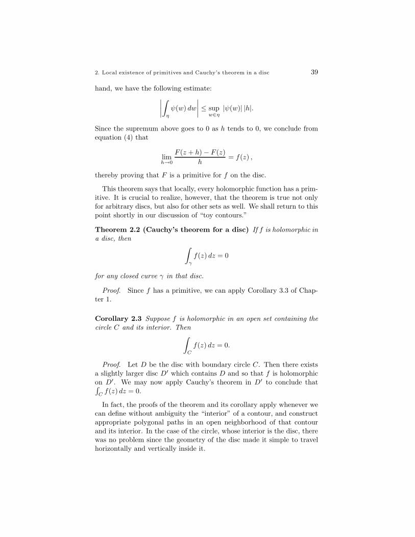
Another important example of a toy contour is the “keyhole” Γ (illus-trated in Figure 5), which we shall put to use in the proof of the Cauchyintegral formula. It consists of two almost complete circles, one large

Γint

Γ

Figure 5. The keyhole contour

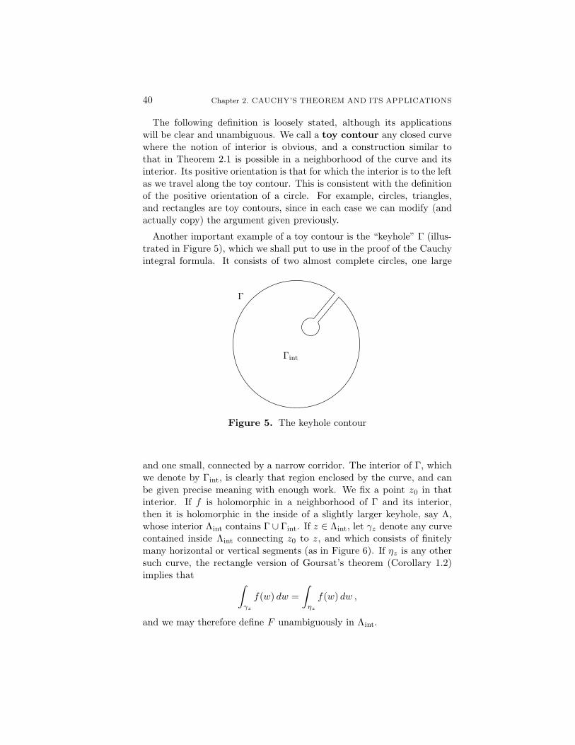
and one small, connected by a narrow corridor. The interior of Γ, whichwe denote by Γint, is clearly that region enclosed by the curve, and canbe given precise meaning with enough work. We fix a point z0 in thatinterior. If f is holomorphic in a neighborhood of Γ and its interior,then it is holomorphic in the inside of a slightly larger keyhole, say Λ,whose interior Λint contains Γ ∪ Γint. If z ∈ Λint, let γz denote any curvecontained inside Λint connecting z0 to z, and which consists of finitelymany horizontal or vertical segments (as in Figure 6). If ηz is any othersuch curve, the rectangle version of Goursat’s theorem (Corollary 1.2)implies that ∫

γz

f(w) dw =

∫

ηz

f(w) dw ,

and we may therefore define F unambiguously in Λint.

3. Evaluation of some integrals 41

Λ

z0

γz

z

Λint

Figure 6. A curve γz

Arguing as above allows us to show that F is a primitive of f in Λint

and therefore∫Γf(z) dz = 0.

The important point is that for a toy contour γ we easily have that

∫

γ

f(z) dz = 0 ,

whenever f is holomorphic in an open set that contains the contour γand its interior.

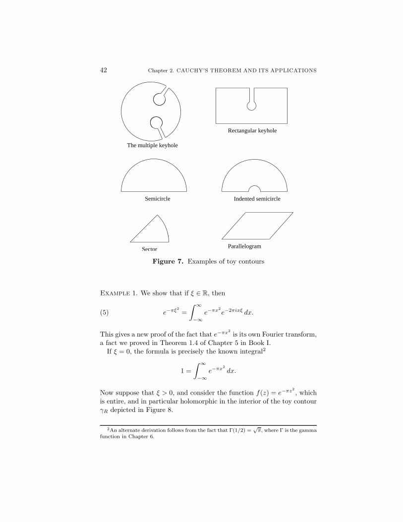
Other examples of toy contours which we shall encounter in applica-tions and for which Cauchy’s theorem and its corollary also hold aregiven in Figure 7.

While Cauchy’s theorem for toy contours is sufficient for most applica-tions we deal with, the question still remains as to what happens for moregeneral curves. We take up this matter in Appendix B, where we proveJordan’s theorem for piecewise-smooth curves. This theorem states thata simple closed piecewise-smooth curve has a well defined interior thatis “simply connected.” As a consequence, we find that even in this moregeneral situation, Cauchy’s theorem holds.

3 Evaluation of some integrals

Here we take up the idea that originally motivated Cauchy. We shallshow by several examples how some integrals may be evaluated by theuse of his theorem. A more systematic approach, in terms of the calculusof residues, may be found in the next chapter.


The multiple keyhole

Semicircle

Sector Parallelogram

Rectangular keyhole

Indented semicircle

Figure 7. Examples of toy contours

Example 1. We show that if ξ ∈ R, then

(5) e−πξ2

=

∫ ∞

−∞e−πx2

e−2πixξ dx.

This gives a new proof of the fact that e−πx2

is its own Fourier transform,a fact we proved in Theorem 1.4 of Chapter 5 in Book I.

If ξ = 0, the formula is precisely the known integral2

1 =

∫ ∞

−∞e−πx2

dx.

Now suppose that ξ > 0, and consider the function f(z) = e−πz2

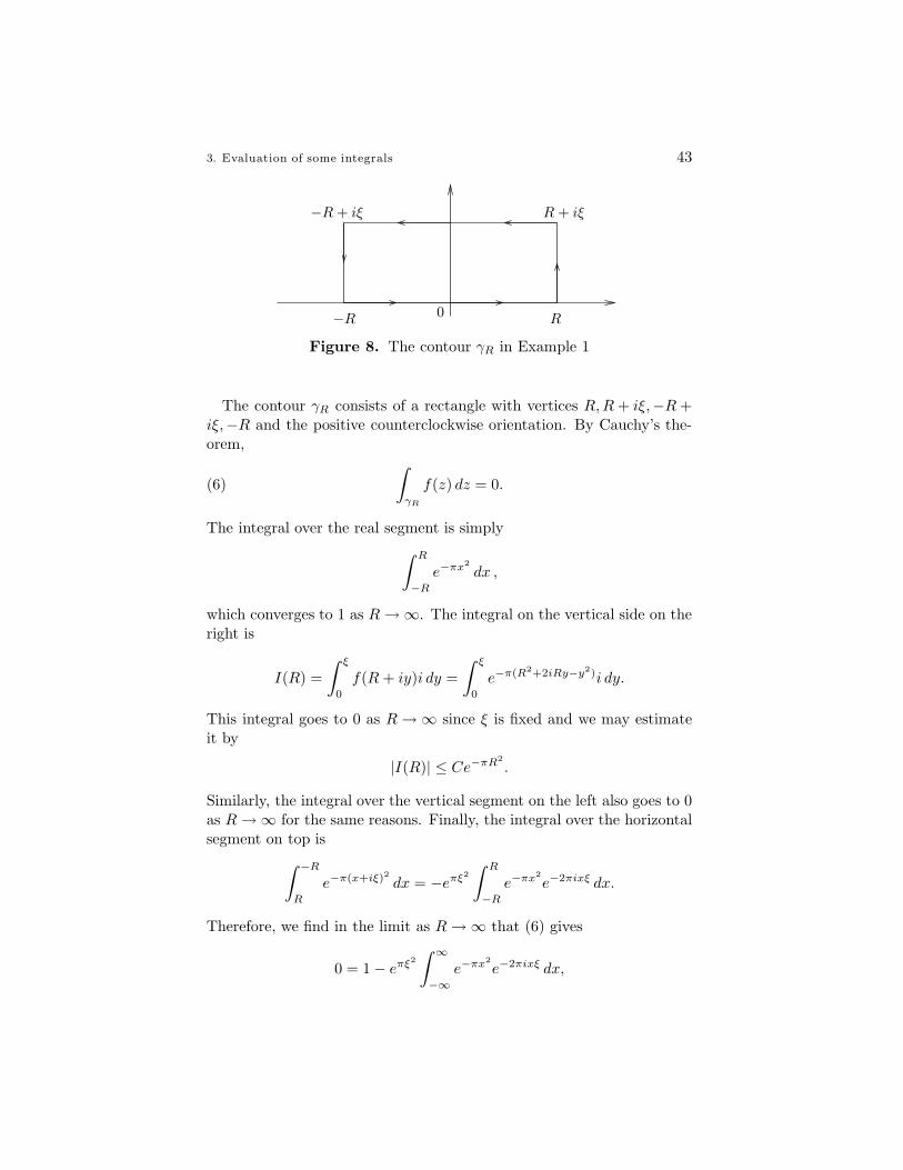
, whichis entire, and in particular holomorphic in the interior of the toy contourγR depicted in Figure 8.

2An alternate derivation follows from the fact that Γ(1/2) =√π, where Γ is the gamma

function in Chapter 6.

3. Evaluation of some integrals 43

R

R + iξ

−R

−R+ iξ

0

Figure 8. The contour γR in Example 1

The contour γR consists of a rectangle with vertices R,R+ iξ,−R+iξ,−R and the positive counterclockwise orientation. By Cauchy’s the-orem,

(6)

∫

γR

f(z) dz = 0.

The integral over the real segment is simply

∫ R

−R

e−πx2

dx ,

which converges to 1 as R→ ∞. The integral on the vertical side on theright is

I(R) =

∫ ξ

0

f(R + iy)i dy =

∫ ξ

0

e−π(R2+2iRy−y2)i dy.

This integral goes to 0 as R→ ∞ since ξ is fixed and we may estimateit by

|I(R)| ≤ Ce−πR2

.

Similarly, the integral over the vertical segment on the left also goes to 0as R→ ∞ for the same reasons. Finally, the integral over the horizontalsegment on top is

∫ −R

R

e−π(x+iξ)2 dx = −eπξ2

∫ R

−R

e−πx2

e−2πixξ dx.

Therefore, we find in the limit as R→ ∞ that (6) gives

0 = 1 − eπξ2

∫ ∞

−∞e−πx2

e−2πixξ dx,


and our desired formula is established. In the case ξ < 0, we then considerthe symmetric rectangle, in the lower half-plane.

The technique of shifting the contour of integration, which was usedin the previous example, has many other applications. Note that theoriginal integral (5) is taken over the real line, which by an applicationof Cauchy’s theorem is then shifted upwards or downwards (dependingon the sign of ξ) in the complex plane.

Example 2. Another classical example is∫ ∞

0

1− cosx

x2dx =

π

2.

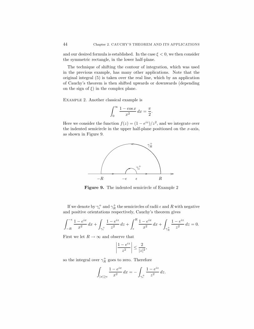
Here we consider the function f(z) = (1 − eiz)/z2, and we integrate overthe indented semicircle in the upper half-plane positioned on the x-axis,as shown in Figure 9.

R

γ+R

−R

γ+ε

ε−ε

Figure 9. The indented semicircle of Example 2

If we denote by γ+ε and γ+

R the semicircles of radii ε and R with negativeand positive orientations respectively, Cauchy’s theorem gives

∫ −ε

−R

1 − eix

x2dx+

∫

γ+ε

1− eiz

z2dz +

∫ R

ε

1 − eix

x2dx+

∫

γ+R

1 − eiz

z2dz = 0.

First we let R→ ∞ and observe that∣∣∣∣1 − eiz

z2

∣∣∣∣ ≤2

|z|2 ,

so the integral over γ+R goes to zero. Therefore

∫

|x|≥ε

1 − eix

x2dx = −

∫

γ+ε

1 − eiz

z2dz.

4. Cauchy’s integral formulas 45

Next, note that

f(z) =−izz2

+E(z)

where E(z) is bounded as z → 0, while on γ+ε we have z = εeiθ and

dz = iεeiθdθ. Thus∫

γ+ε

1 − eiz

z2dz →

∫ 0

π

(−ii) dθ = −π as ε→ 0.

Taking real parts then yields∫ ∞

−∞

1 − cosx

x2dx = π.

Since the integrand is even, the desired formula is proved.

4 Cauchy’s integral formulas

Representation formulas, and in particular integral representation formu-las, play an important role in mathematics, since they allow us to recovera function on a large set from its behavior on a smaller set. For example,we saw in Book I that a solution of the steady-state heat equation in thedisc was completely determined by its boundary values on the circle viaa convolution with the Poisson kernel

(7) u(r, θ) =1

2π

∫ 2π

0

Pr(θ − ϕ)u(1, ϕ) dϕ.

In the case of holomorphic functions, the situation is analogous, whichis not surprising since the real and imaginary parts of a holomorphicfunction are harmonic.3 Here, we will prove an integral representationformula in a manner that is independent of the theory of harmonic func-tions. In fact, it is also possible to recover the Poisson integral formula (7)as a consequence of the next theorem (see Exercises 11 and 12).

Theorem 4.1 Suppose f is holomorphic in an open set that containsthe closure of a disc D. If C denotes the boundary circle of this disc withthe positive orientation, then

f(z) =1

2πi

∫

C

f(ζ)

ζ − zdζ for any point z ∈ D.

3This fact is an immediate consequence of the Cauchy-Riemann equations. We referthe reader to Exercise 11 in Chapter 1.


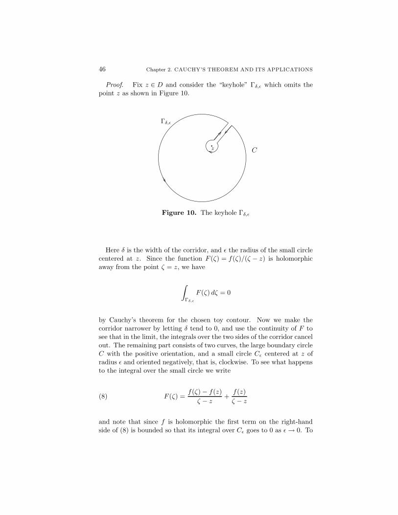
Proof. Fix z ∈ D and consider the “keyhole” Γδ,ε which omits thepoint z as shown in Figure 10.

Γδ,ε

z C

Figure 10. The keyhole Γδ,ε

Here δ is the width of the corridor, and ε the radius of the small circlecentered at z. Since the function F (ζ) = f(ζ)/(ζ − z) is holomorphicaway from the point ζ = z, we have

∫

Γδ,ε

F (ζ) dζ = 0

by Cauchy’s theorem for the chosen toy contour. Now we make thecorridor narrower by letting δ tend to 0, and use the continuity of F tosee that in the limit, the integrals over the two sides of the corridor cancelout. The remaining part consists of two curves, the large boundary circleC with the positive orientation, and a small circle Cε centered at z ofradius ε and oriented negatively, that is, clockwise. To see what happensto the integral over the small circle we write

(8) F (ζ) =f(ζ) − f(z)

ζ − z+f(z)

ζ − z

and note that since f is holomorphic the first term on the right-handside of (8) is bounded so that its integral over Cε goes to 0 as ε→ 0. To


conclude the proof, it suffices to observe that

∫

Cε

f(z)

ζ − zdζ = f(z)

∫

Cε

dζ

ζ − z

= −f(z)

∫ 2π

0

εie−it

εe−itdt

= −f(z)2πi ,

so that in the limit we find

0 =

∫

C

f(ζ)

ζ − zdζ − 2πif(z) ,

as was to be shown.

Remarks. Our earlier discussion of toy contours provides simple ex-tensions of the Cauchy integral formula; for instance, if f is holomorphicin an open set that contains a (positively oriented) rectangle R and itsinterior, then

f(z) =1

2πi

∫

R

f(ζ)

ζ − zdζ ,

whenever z belongs to the interior ofR. To establish this result, it sufficesto repeat the proof of Theorem 4.1 replacing the “circular” keyhole by a“rectangular” keyhole.

It should also be noted that the above integral vanishes when z isoutside R, since in this case F (ζ) = f(ζ)/(ζ − z) is holomorphic insideR. Of course, a similar result also holds for the circle or any other toycontour.

As a corollary to the Cauchy integral formula, we arrive at a secondremarkable fact about holomorphic functions, namely their regularity.We also obtain further integral formulas expressing the derivatives of finside the disc in terms of the values of f on the boundary.

Corollary 4.2 If f is holomorphic in an open set Ω, then f has infinitelymany complex derivatives in Ω. Moreover, if C ⊂ Ω is a circle whoseinterior is also contained in Ω, then

f (n)(z) =n!

2πi

∫

C

f(ζ)

(ζ − z)n+1dζ

for all z in the interior of C.


We recall that, as in the above theorem, we take the circle C to havepositive orientation.

Proof. The proof is by induction on n, the case n = 0 being simplythe Cauchy integral formula. Suppose that f has up to n− 1 complexderivatives and that

f (n−1)(z) =(n− 1)!

2πi

∫

C

f(ζ)

(ζ − z)ndζ.

Now for h small, the difference quotient for f (n−1) takes the form

(9)f (n−1)(z + h) − f (n−1)(z)

h=

(n− 1)!

2πi

∫

C

f(ζ)1

h

[1

(ζ − z − h)n− 1

(ζ − z)n

]dζ.

We now recall that

An − Bn = (A−B)[An−1 +An−2B + · · · +ABn−2 +Bn−1].

With A = 1/(ζ − z − h) and B = 1/(ζ − z), we see that the term inbrackets in equation (9) is equal to

h

(ζ − z − h)(ζ − z)[An−1 +An−2B + · · · +ABn−2 +Bn−1].

But observe that if h is small, then z + h and z stay at a finite distancefrom the boundary circle C, so in the limit as h tends to 0, we find thatthe quotient converges to

(n− 1)!

2πi

∫

C

f(ζ)

[1

(ζ − z)2

][n

(ζ − z)n−1

]dζ =

n!

2πi

∫

C

f(ζ)

(ζ − z)n+1dζ ,

which completes the induction argument and proves the theorem.

From now on, we call the formulas of Theorem 4.1 and Corollary 4.2the Cauchy integral formulas.

Corollary 4.3 (Cauchy inequalities) If f is holomorphic in an openset that contains the closure of a disc D centered at z0 and of radius R,then

|f (n)(z0)| ≤n!‖f‖C

Rn,

where ‖f‖C = supz∈C |f(z)| denotes the supremum of |f | on the boundarycircle C.


Proof. Applying the Cauchy integral formula for f (n)(z0), we obtain

|f (n)(z0)| =

∣∣∣∣n!

2πi

∫

C

f(ζ)

(ζ − z0)n+1dζ

∣∣∣∣

=n!

2π

∣∣∣∣∫ 2π

0

f(z0 +Reiθ)

(Reiθ)n+1Rieiθ dθ

∣∣∣∣

≤ n!

2π

‖f‖C

Rn2π.

Another striking consequence of the Cauchy integral formula is itsconnection with power series. In Chapter 1, we proved that a power seriesis holomorphic in the interior of its disc of convergence, and promised aproof of a converse, which is the content of the next theorem.

Theorem 4.4 Suppose f is holomorphic in an open set Ω. If D is adisc centered at z0 and whose closure is contained in Ω, then f has apower series expansion at z0

f(z) =

∞∑

n=0

an(z − z0)n

for all z ∈ D, and the coefficients are given by

an =f (n)(z0)

n!for all n ≥ 0.

Proof. Fix z ∈ D. By the Cauchy integral formula, we have

(10) f(z) =1

2πi

∫

C

f(ζ)

ζ − zdζ ,

where C denotes the boundary of the disc and z ∈ D. The idea is towrite

(11)1

ζ − z=

1

ζ − z0 − (z − z0)=

1

ζ − z0

1

1 −(

z−z0

ζ−z0

) ,

and use the geometric series expansion. Since ζ ∈ C and z ∈ D is fixed,there exists 0 < r < 1 such that

∣∣∣∣z − z0ζ − z0

∣∣∣∣ < r,


therefore

(12)1

1−(

z−z0

ζ−z0

) =

∞∑

n=0

(z − z0ζ − z0

)n

,

where the series converges uniformly for ζ ∈ C. This allows us to inter-change the infinite sum with the integral when we combine (10), (11),and (12), thereby obtaining

f(z) =

∞∑

n=0

(1

2πi

∫

C

f(ζ)

(ζ − z0)n+1dζ

)· (z − z0)

n.

This proves the power series expansion; further the use of the Cauchy in-tegral formulas for the derivatives (or simply differentiation of the series)proves the formula for an.

Observe that since power series define indefinitely (complex) differ-entiable functions, the theorem gives another proof that a holomorphicfunction is automatically indefinitely differentiable.

Another important observation is that the power series expansion off centered at z0 converges in any disc, no matter how large, as longas its closure is contained in Ω. In particular, if f is entire (that is,holomorphic on all of C), the theorem implies that f has a power seriesexpansion around 0, say f(z) =

∑∞n=0 anz

n, that converges in all of C.

Corollary 4.5 (Liouville’s theorem) If f is entire and bounded, thenf is constant.

Proof. It suffices to prove that f ′ = 0, since C is connected, and wemay then apply Corollary 3.4 in Chapter 1.

For each z0 ∈ C and all R > 0, the Cauchy inequalities yield

|f ′(z0)| ≤B

R

where B is a bound for f . Letting R→ ∞ gives the desired result.

As an application of our work so far, we can give an elegant proof ofthe fundamental theorem of algebra.

Corollary 4.6 Every non-constant polynomial P (z) = anzn + · · · + a0

with complex coefficients has a root in C.

Proof. If P has no roots, then 1/P (z) is a bounded holomorphicfunction. To see this, we can of course assume that an 6= 0, and write

P (z)

zn= an +

(an−1

z+ · · · + a0

zn

)


whenever z 6= 0. Since each term in the parentheses goes to 0 as |z| → ∞we conclude that there exists R > 0 so that if c = |an|/2, then

|P (z)| ≥ c|z|n whenever |z| > R.

In particular, P is bounded from below when |z| > R. Since P is contin-uous and has no roots in the disc |z| ≤ R, it is bounded from below inthat disc as well, thereby proving our claim.

By Liouville’s theorem we then conclude that 1/P is constant. Thiscontradicts our assumption that P is non-constant and proves the corol-lary.

Corollary 4.7 Every polynomial P (z) = anzn + · · · + a0 of degree n ≥

1 has precisely n roots in C. If these roots are denoted by w1, . . . , wn,then P can be factored as

P (z) = an(z − w1)(z − w2) · · · (z − wn).

Proof. By the previous result P has a root, say w1. Then, writingz = (z − w1) + w1, inserting this expression for z in P , and using thebinomial formula we get

P (z) = bn(z − w1)n + · · · + b1(z − w1) + b0,

where b0, . . . , bn−1 are new coefficients, and bn = an. Since P (w1) = 0,we find that b0 = 0, therefore

P (z) = (z − w1)[bn(z − w1)

n−1 + · · · + b1]

= (z − w1)Q(z),

where Q is a polynomial of degree n− 1. By induction on the degree ofthe polynomial, we conclude that P (z) has n roots and can be expressedas

P (z) = c(z − w1)(z − w2) · · · (z − wn)

for some c ∈ C. Expanding the right-hand side, we realize that the coef-ficient of zn is c and therefore c = an as claimed.

Finally, we end this section with a discussion of analytic continuation(the third of the “miracles” we mentioned in the introduction). It statesthat the “genetic code” of a holomorphic function is determined (thatis, the function is fixed) if we know its values on appropriate arbitrarilysmall subsets. Note that in the theorem below, Ω is assumed connected.


Theorem 4.8 Suppose f is a holomorphic function in a region Ω thatvanishes on a sequence of distinct points with a limit point in Ω. Thenf is identically 0.

In other words, if the zeros of a holomorphic function f in the con-nected open set Ω accumulate in Ω, then f = 0.

Proof. Suppose that z0 ∈ Ω is a limit point for the sequence wk∞k=1

and that f(wk) = 0. First, we show that f is identically zero in a smalldisc containing z0. For that, we choose a disc D centered at z0 andcontained in Ω, and consider the power series expansion of f in that disc

f(z) =

∞∑

n=0

an(z − z0)n.

If f is not identically zero, there exists a smallest integer m such thatam 6= 0. But then we can write

f(z) = am(z − z0)m(1 + g(z − z0)),

where g(z − z0) converges to 0 as z → z0. Taking z = wk 6= z0 for a se-quence of points converging to z0, we get a contradiction sinceam(wk − z0)

m 6= 0 and 1 + g(wk − z0) 6= 0, but f(wk) = 0.We conclude the proof using the fact that Ω is connected. Let U

denote the interior of the set of points where f(z) = 0. Then U is openby definition and non-empty by the argument just given. The set U isalso closed since if zn ∈ U and zn → z, then f(z) = 0 by continuity, andf vanishes in a neighborhood of z by the argument above. Hence z ∈ U .Now if we let V denote the complement of U in Ω, we conclude that Uand V are both open, disjoint, and

Ω = U ∪ V.

Since Ω is connected we conclude that either U or V is empty. (Here weuse one of the two equivalent definitions of connectedness discussed inChapter 1.) Since z0 ∈ U , we find that U = Ω and the proof is complete.

An immediate consequence of the theorem is the following.

Corollary 4.9 Suppose f and g are holomorphic in a region Ω andf(z) = g(z) for all z in some non-empty open subset of Ω (or more gen-erally for z in some sequence of distinct points with limit point in Ω).Then f(z) = g(z) throughout Ω.

5. Further applications 53

Suppose we are given a pair of functions f and F analytic in regionsΩ and Ω′, respectively, with Ω ⊂ Ω′. If the two functions agree on thesmaller set Ω, we say that F is an analytic continuation of f into theregion Ω′. The corollary then guarantees that there can be only one suchanalytic continuation, since F is uniquely determined by f .

5 Further applications

We gather in this section various consequences of the results proved sofar.

5.1 Morera’s theorem

A direct application of what was proved here is a converse of Cauchy’stheorem.

Theorem 5.1 Suppose f is a continuous function in the open disc Dsuch that for any triangle T contained in D

∫

T

f(z) dz = 0,

then f is holomorphic.

Proof. By the proof of Theorem 2.1 the function f has a primitive Fin D that satisfies F ′ = f . By the regularity theorem, we know that Fis indefinitely (and hence twice) complex differentiable, and therefore fis holomorphic.

5.2 Sequences of holomorphic functions

Theorem 5.2 If fn∞n=1 is a sequence of holomorphic functions thatconverges uniformly to a function f in every compact subset of Ω, thenf is holomorphic in Ω.

Proof. Let D be any disc whose closure is contained in Ω and Tany triangle in that disc. Then, since each fn is holomorphic, Goursat’stheorem implies

∫

T

fn(z) dz = 0 for all n.

By assumption fn → f uniformly in the closure of D, so f is continuousand ∫

T

fn(z) dz →∫

T

f(z) dz.

Documents

Elias M. Stein and Rami Shakarchi: Complex Analysisassets.press.princeton.edu/chapters/s02_7563.pdf · Elias M. Stein and Rami Shakarchi: Complex Analysis . 2 Cauchy’s Theorem and