ELEN0019:

Audio signal processing.

Principles and experiments

ELEN0019 - 2014

• To give an introduction to digital signal processing in

audio applications,

• Emphasis is on real-time applications, through the

programming of a DSP (digital signal processor),

• Laboratory sessions: the students will have the

opportunity to design their own systems, to test their

operation through measurements and listening !

• Textbook: http://www.montefiore.ulg.ac.be/~josmalskyj/dsp.php

ELEN0019 - 2014

Course objectives

• Specific processors optimized for real-time signal

processing,

• Example: the MAC operation (multiply and accumulate),

mostly used in the convolution operations,

• The Harvard architecture of the processor allows to read

an instruction and the corresponding data in memory, in

one clock cycle.

ELEN0019 - 2014

Digital signal processors (I)

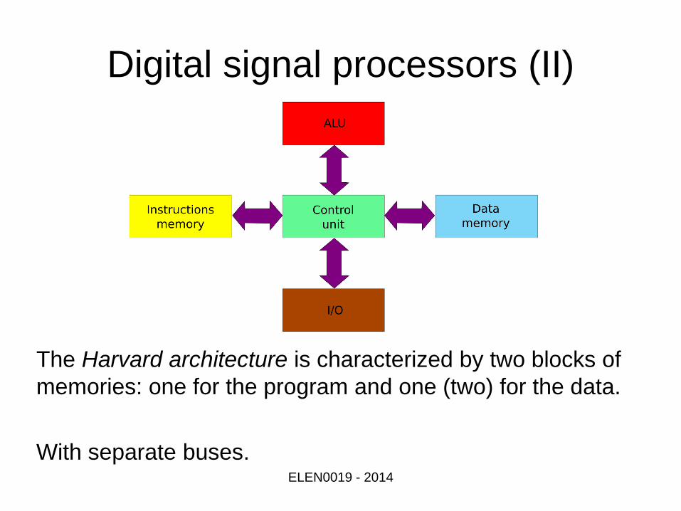
The Harvard architecture is characterized by two blocks of

memories: one for the program and one (two) for the data.

With separate buses.

ELEN0019 - 2014

Digital signal processors (II)

ELEN0019 - 2014

Digital signal processors (III)

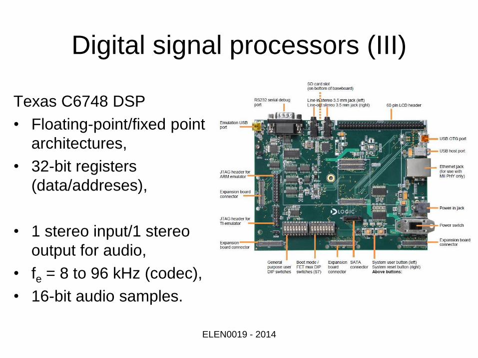
Texas C6748 DSP

• Floating-point/fixed point

architectures,

• 32-bit registers

(data/addreses),

• 1 stereo input/1 stereo

output for audio,

• fe = 8 to 96 kHz (codec),

• 16-bit audio samples.

ELEN0019 - 2014

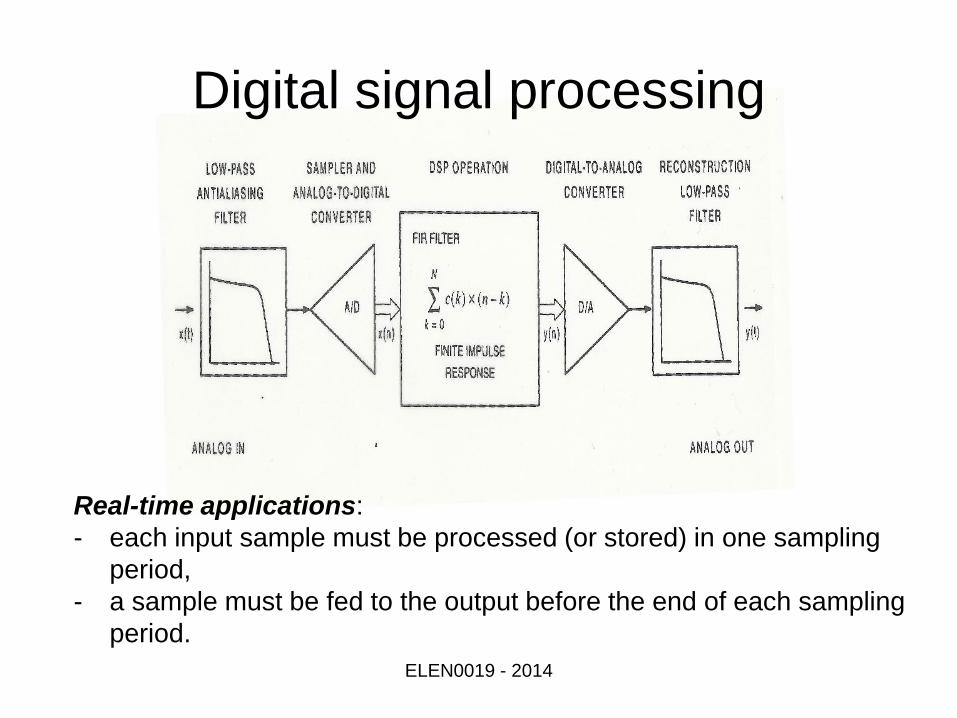
Digital signal processing

Real-time applications:

- each input sample must be processed (or stored) in one sampling

period,

- a sample must be fed to the output before the end of each sampling

period.

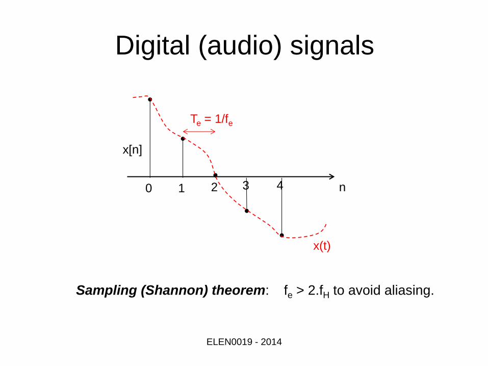
Digital (audio) signals

ELEN0019 - 2014

Sampling (Shannon) theorem: fe > 2.fH to avoid aliasing.

n 0 1 3 2 4

x[n]

x(t)

Te = 1/fe

Digital (audio) filters (I)

y[n] FILTER

EXCITATION

(INPUT)

RESPONSE

(OUTPUT)

CAUSALITY: if x[n]=0 for n<n0, then y[n]=0 for n<n0

LINEAR AND TIME-INVARIANT (LTI) SYSTEMS:

b0 y[n] + … bN y[n-N] = a0 x[n] + … aM x[n-M]

ELEN0019 - 2014

x[n] n 0 1 3 2 4

STABILITY : y[n] bounded if x[n] bounded

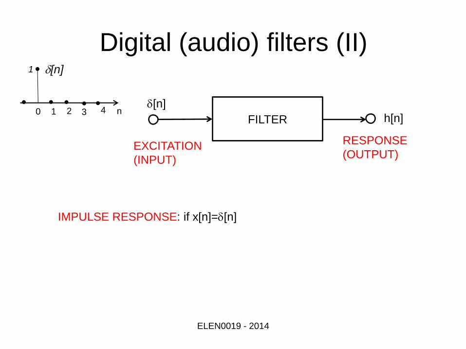
Digital (audio) filters (II)

h[n] FILTER

EXCITATION

(INPUT)

RESPONSE

(OUTPUT)

IMPULSE RESPONSE: if x[n]=d[n]

ELEN0019 - 2014

d[n] n 0 1 3 2 4

1 d[n]

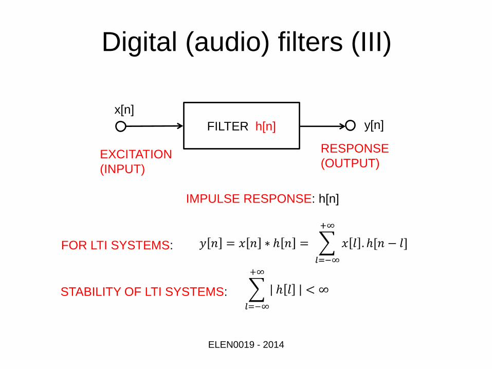
Digital (audio) filters (III)

y[n] FILTER h[n]

EXCITATION

(INPUT)

RESPONSE

(OUTPUT)

IMPULSE RESPONSE: h[n]

ELEN0019 - 2014

x[n]

FOR LTI SYSTEMS:

STABILITY OF LTI SYSTEMS:

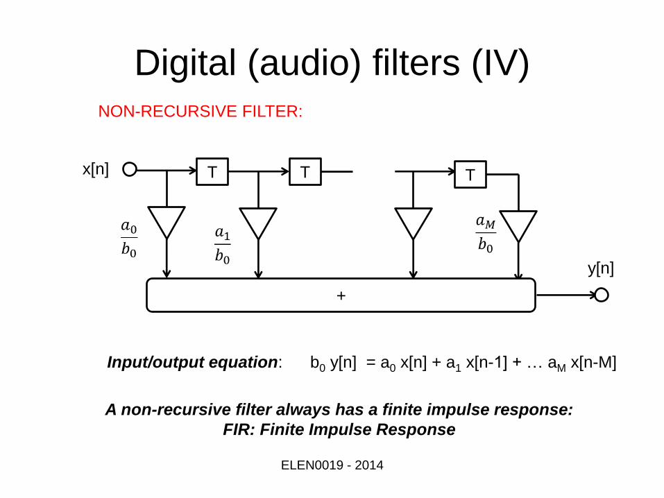
Digital (audio) filters (IV) NON-RECURSIVE FILTER:

A non-recursive filter always has a finite impulse response:

FIR: Finite Impulse Response

x[n]

y[n]

T T T

+

ELEN0019 - 2014

Input/output equation: b0 y[n] = a0 x[n] + a1 x[n-1] + … aM x[n-M]

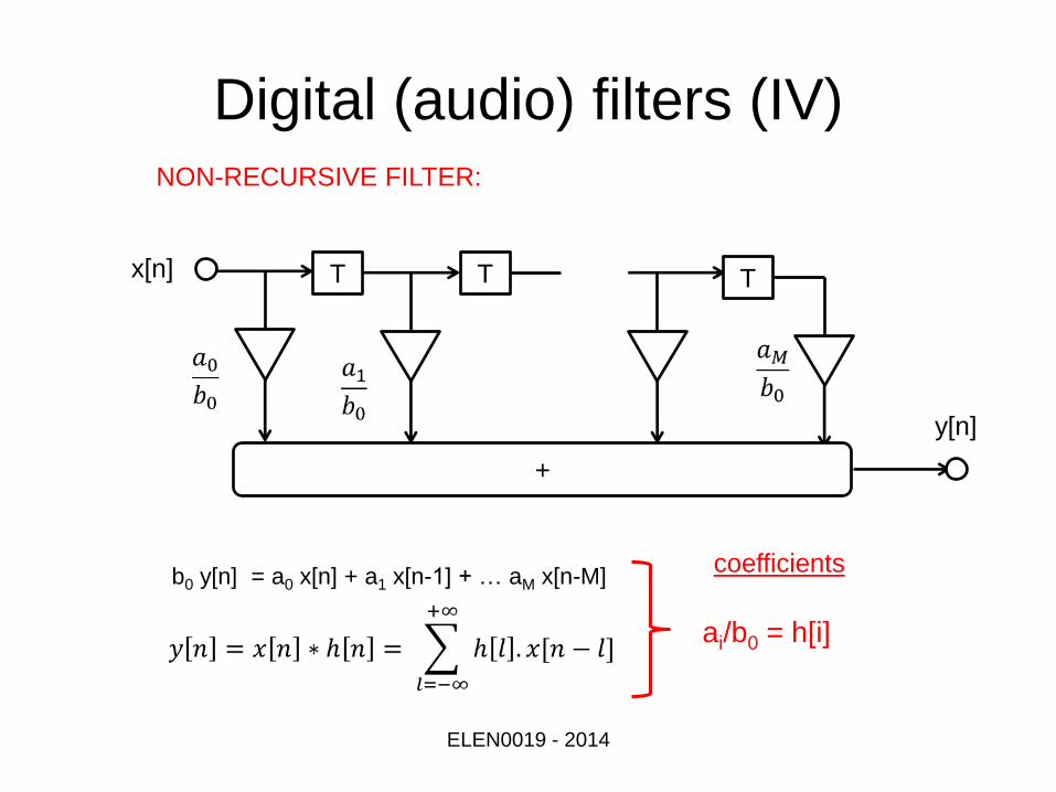
Digital (audio) filters (IV) NON-RECURSIVE FILTER:

x[n]

y[n]

T T T

+

ELEN0019 - 2014

b0 y[n] = a0 x[n] + a1 x[n-1] + … aM x[n-M]

ai/b0 = h[i]

coefficients

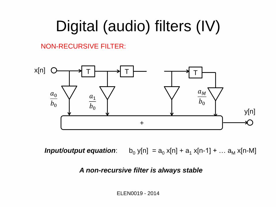
Digital (audio) filters (IV) NON-RECURSIVE FILTER:

A non-recursive filter is always stable

x[n]

y[n]

T T T

+

ELEN0019 - 2014

Input/output equation: b0 y[n] = a0 x[n] + a1 x[n-1] + … aM x[n-M]

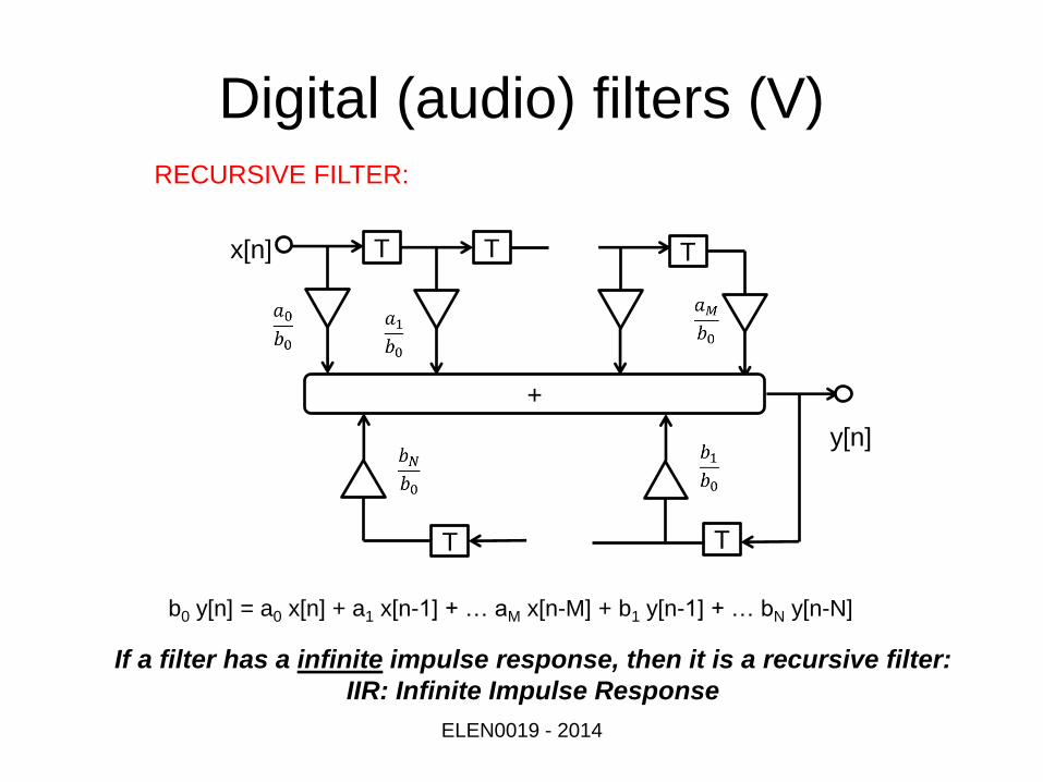
Digital (audio) filters (V) RECURSIVE FILTER:

T

x[n]

y[n]

T T T

+

T

ELEN0019 - 2014

b0 y[n] = a0 x[n] + a1 x[n-1] + … aM x[n-M] + b1 y[n-1] + … bN y[n-N]

If a filter has a infinite impulse response, then it is a recursive filter:

IIR: Infinite Impulse Response

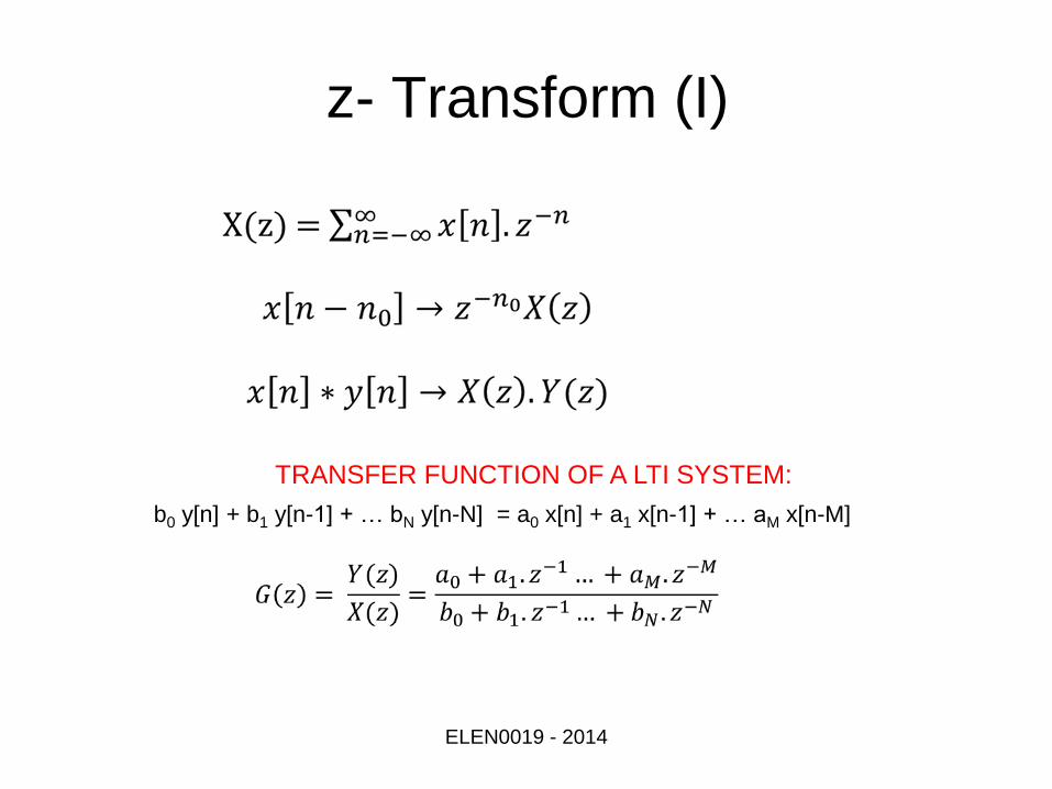
z- Transform (I)

TRANSFER FUNCTION OF A LTI SYSTEM:

ELEN0019 - 2014

b0 y[n] + b1 y[n-1] + … bN y[n-N] = a0 x[n] + a1 x[n-1] + … aM x[n-M]

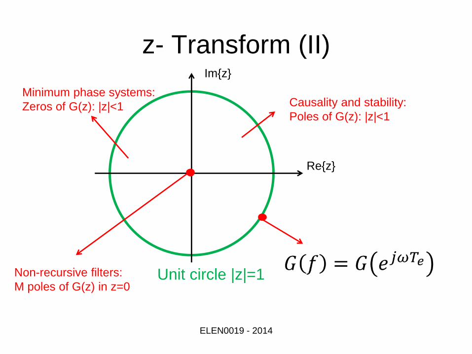
z- Transform (II)

Re{z}

Im{z}

Causality and stability:

Poles of G(z): |z|<1

Minimum phase systems:

Zeros of G(z): |z|<1

Unit circle |z|=1 Non-recursive filters:

M poles of G(z) in z=0

ELEN0019 - 2014

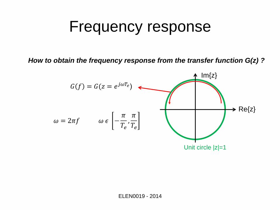
Frequency response

ELEN0019 - 2014

How to obtain the frequency response from the transfer function G(z) ?

Re{z}

Im{z}

Unit circle |z|=1

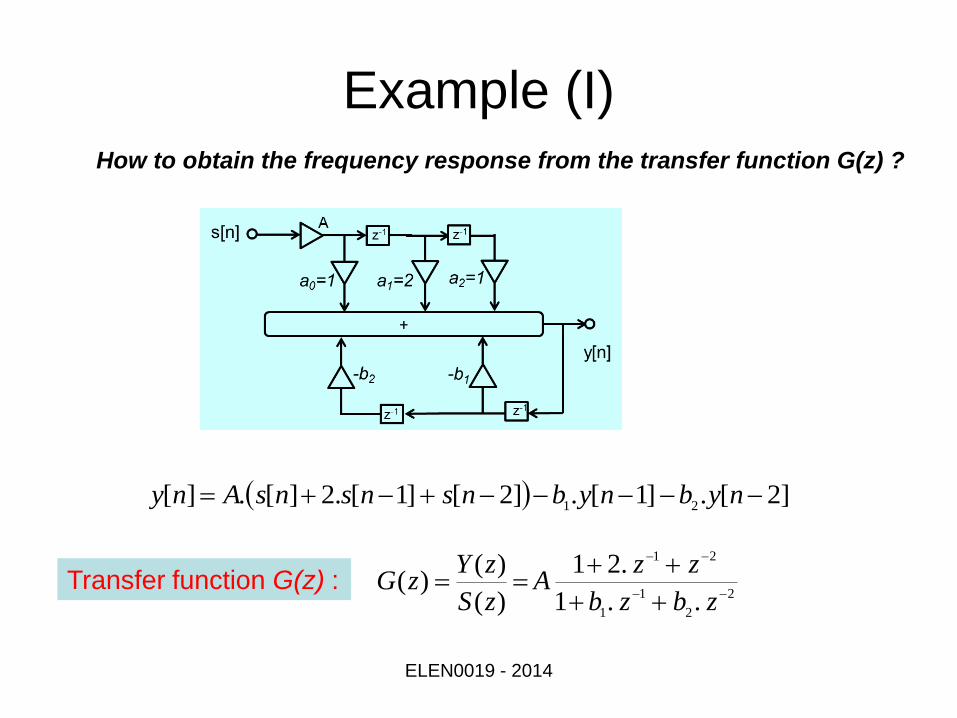
Example (I)

ELEN0019 - 2014

How to obtain the frequency response from the transfer function G(z) ?

]2[.]1[.]2[]1[.2][.][21

nybnybnsnsnsAny

Transfer function G(z) : 2

2

1

1

21

..1

.21

)(

)()(

zbzb

zzA

zS

zYzG

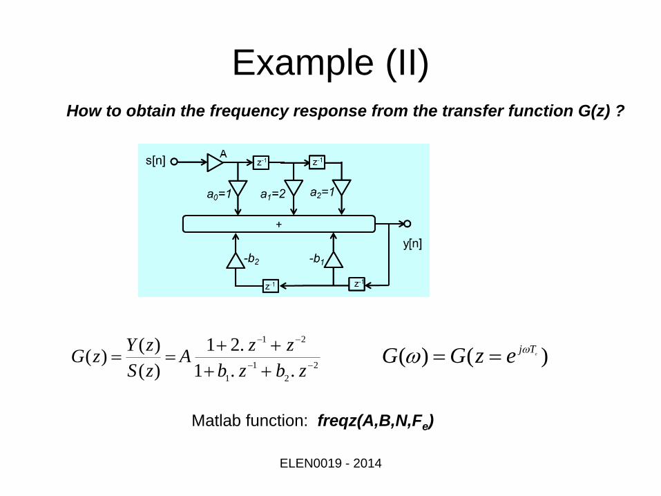
Example (II)

ELEN0019 - 2014

How to obtain the frequency response from the transfer function G(z) ?

2

2

1

1

21

..1

.21

)(

)()(

zbzb

zzA

zS

zYzG )()( e

TjezGG

Matlab function: freqz(A,B,N,Fe)

Example (III)

ELEN0019 - 2014

How to obtain the frequency response from the transfer function G(z) ?

• A = 0,005542

• b1 = -1,7786,

• b2 = -0,8008,

• fe = 48 kHz.

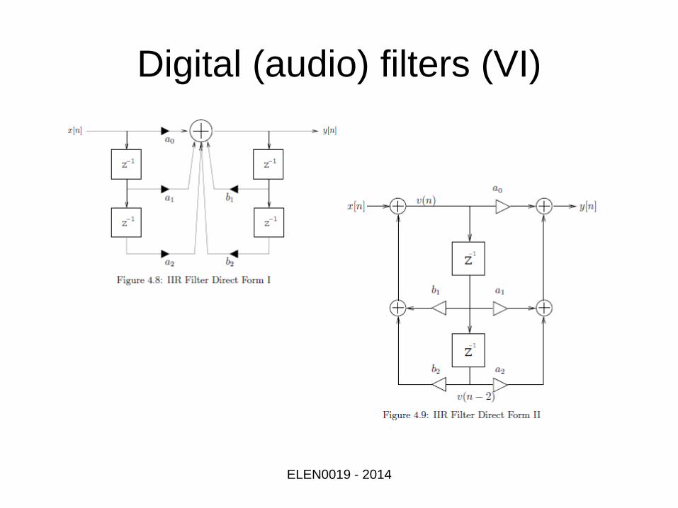
Digital (audio) filters (VI)

ELEN0019 - 2014