Embed Size (px)
Citation preview
Elements of Statistical Mechanics and
Large Deviation Theory

Contents
Chapter 1. Introduction . . . . . . . . . . . . . . . . . . . . . . . . . . . 11. Equilibrium Statistical Mechanics . . . . . . . . . . . . . . . . . . . 12. Large deviations . . . . . . . . . . . . . . . . . . . . . . . . . . . . . 53. Spin systems . . . . . . . . . . . . . . . . . . . . . . . . . . . . . . . 8
Chapter 2. The Maximum Entropy Principle . . . . . . . . . . . . . . . . 91. The Gibbs Distribution . . . . . . . . . . . . . . . . . . . . . . . . . 132. Uniqueness of Entropy . . . . . . . . . . . . . . . . . . . . . . . . . 16
Chapter 3. Large Deviations for finite alphabets . . . . . . . . . . . . . . 211. The Theorem of Sanov . . . . . . . . . . . . . . . . . . . . . . . . . 212. Applications . . . . . . . . . . . . . . . . . . . . . . . . . . . . . . . 273. The Theorem of Sanov for Pairs . . . . . . . . . . . . . . . . . . . . 34
Chapter 4. The Ideal Gas . . . . . . . . . . . . . . . . . . . . . . . . . . 371. The Microcanonical Distribution . . . . . . . . . . . . . . . . . . . . 382. The equilibrium value of the kinetic energy . . . . . . . . . . . . . . 403. The equilibrium value of other observables . . . . . . . . . . . . . . 42
Chapter 5. The Large Deviation Principle . . . . . . . . . . . . . . . . . 431. Definition of the LDP . . . . . . . . . . . . . . . . . . . . . . . . . . 432. The Varadhan Lemma . . . . . . . . . . . . . . . . . . . . . . . . . 473. LDP for Tilted Measures . . . . . . . . . . . . . . . . . . . . . . . . 484. The Contraction Principle . . . . . . . . . . . . . . . . . . . . . . . 49
Chapter 6. The Curie-Weiss Model . . . . . . . . . . . . . . . . . . . . . 511. The LDP for the magnetization . . . . . . . . . . . . . . . . . . . . 522. The free energy . . . . . . . . . . . . . . . . . . . . . . . . . . . . . 54
Chapter 7. The Theorem of Cramer . . . . . . . . . . . . . . . . . . . . . 551. The logarithmic moment generating function . . . . . . . . . . . . . 552. Main Theorem . . . . . . . . . . . . . . . . . . . . . . . . . . . . . . 563. The Theorem of Cramer in R
d . . . . . . . . . . . . . . . . . . . . . 60
Chapter 8. The Ising Model (COMPLETER) . . . . . . . . . . . . . . . 611. The FKG Inequality . . . . . . . . . . . . . . . . . . . . . . . . . . . 622. The thermodynamic limit . . . . . . . . . . . . . . . . . . . . . . . . 623. Proofs . . . . . . . . . . . . . . . . . . . . . . . . . . . . . . . . . . 64
Chapter 9. The DLR Formalism . . . . . . . . . . . . . . . . . . . . . . . 671. Random Fields via Kolmogorov’s Extension Theorem . . . . . . . . 67
iii
iv CONTENTS
2. Random Fields via Specifications . . . . . . . . . . . . . . . . . . . . 683. The Ising model, again . . . . . . . . . . . . . . . . . . . . . . . . . 734. An Inhomogeneous Ising chain on N . . . . . . . . . . . . . . . . . . 735. Uniqueness; Dobrushin’s Condition of Weak Dependence . . . . . . 74
Chapter 10. The Variational Principle . . . . . . . . . . . . . . . . . . . . 831. Introduction . . . . . . . . . . . . . . . . . . . . . . . . . . . . . . . 832. The Entropy of an Invariant Random Field . . . . . . . . . . . . . . 853. Gibbs measures as reference measures . . . . . . . . . . . . . . . . . 88
Chapter 11. Gibbs Measures and Large Deviations . . . . . . . . . . . . . 951. Introduction . . . . . . . . . . . . . . . . . . . . . . . . . . . . . . . 952. The Free Gibbs Measure . . . . . . . . . . . . . . . . . . . . . . . . 963. The LDP for Ln under the product measure . . . . . . . . . . . . . 974. The LDP for Ln under the Free Gibbs measure . . . . . . . . . . . . 107
Bibliography . . . . . . . . . . . . . . . . . . . . . . . . . . . . . . . . . . 109
Index . . . . . . . . . . . . . . . . . . . . . . . . . . . . . . . . . . . . . . 111
CHAPTER 1
Introduction
These notes aim at presenting some aspects of two intimately related areas,namely Equilibirum Statistical Mechanics (ESM) and Large Deviation Theory(LDT). On one side, ESM defines and studies the probability measures associ-ated to large systems of particles. On the other, LDT is a classical chapter ofprobability theory which can be loosely described as a refinement of the Lawof Large Numbers. I will try to introduce concepts from both sides in the mostnatural way, and show what are their common features. The text does not aim atpresenting the most general results, but rather at going deeper into the richnessof a few examples, such as random variables with values in a finite alphabets,which, in the statistical mechanics language, amounts to restrict to lattice spinsystems.
The material presented in these notes is taken from a series of standard texts onthe subject. There are two references that cover both LDT and ESM: [Ell85,OV05]. For LDT, the main references are [dH00, Lan73, DZ98, Str84, LP95].A non-technical reference, which covers a few aspects of the material in thesimplest way, is [CT06]. Concerning ESM, some basic references are [Geo75,
Geo88, Jay63, ML79, Pre76]. Finally, a series of papers on equivalence ofensembles will be exposed: [LPS95, LPS94]. [Var66, Roc97, Cra38] In thisintroduction I briefly describe what will be the main lines followed in the notes.
1. Equilibrium Statistical Mechanics
Consider for example a gas 1, composed of a large number of identical particles,say n = 1025. Statistical mechanics is concerned with giving a reasonable de-scription of such a large system. By a reasonable description, we mean a theorycapable of making prediction about some properties of the system, like how thegas will react to external forces or thermodynamic changes. Since the gas is madeof particles, knowing the state of each particle is equivalent to knowing the stateof the gas. Therefore, we can assume that a perfect knowledge of the system ata given time t is a vector
x(t) = (q1(t), p1(t), . . . , qn(t), pn(t)) ∈ (R3 × R3)n ≃ R
6n ,
1We will give a detailed analysis of the model presented here in Chapter 4. The informaldiscussion of this introduction also applies to other systems, such as ferromagnets, which willalso be considered later.
1
2 1. INTRODUCTION
giving the position qi(t) ∈ R3 and a momentum pi(t) ∈ R
3 of each particle. If aninitial confition x0 ∈ R
6n is fixed, i.e. x0 = x(t = 0), Classical Newtonian me-chanics gives, in principle, a way of knowing x(t) for each t > 0. If the interactionpotential among the particles is given (and not too singular), then x(t) is solutionof a system of R6n first order differential equations (Newton Equations). Unlessthe potential is trivial, or if the initial condition has pathological features, solvingthis differential system and obtaining explicit information on the time evolutionseems a rather tough analytic problem.
But before even opening a textbook on ordinary differential equations, the readermust agree that solving exactly the above system is not what one wants to do,for the following reasons.
First, the exact microscopic position of each atom in a gas is not a particularlyexciting piece of information, since our aim is to describe more relevant observ-ables related to the global behaviour of the system (see Un hereafter). In orderto solve the above system of differential equations, one must also determine theinitial condition x0 which in itself should be considered as impossible, at leastexperimentally.
Second, we can start by restricting our attention to particular conditions. A sim-ple but interesting one is the one which consists in waiting for the gas to havereached equilibrium. This amounts to study the limit t → ∞. From the analyt-ical point of view mentionned before, this limit seems to be even more difficult(existence of solutions to differential equations are typically guaranteed over fi-nite time intervals), but the system seems nevertheless simpler to describe oncea certain equilibrium has been reached.
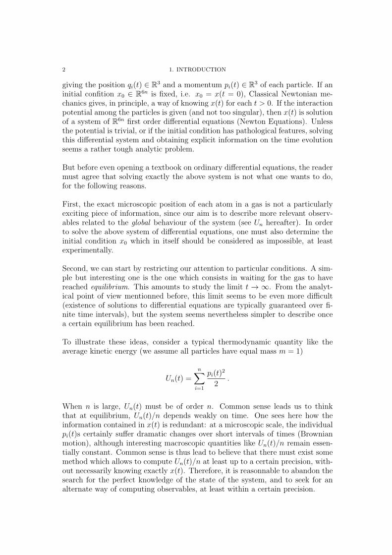
To illustrate these ideas, consider a typical thermodynamic quantity like theaverage kinetic energy (we assume all particles have equal mass m = 1)
Un(t) =n∑
i=1
pi(t)2
2.
When n is large, Un(t) must be of order n. Common sense leads us to thinkthat at equilibrium, Un(t)/n depends weakly on time. One sees here how theinformation contained in x(t) is redundant: at a microscopic scale, the individualpi(t)s certainly suffer dramatic changes over short intervals of times (Brownianmotion), although interesting macroscopic quantities like Un(t)/n remain essen-tially constant. Common sense is thus lead to believe that there must exist somemethod which allows to compute Un(t)/n at least up to a certain precision, with-out necessarily knowing exactly x(t). Therefore, it is reasonnable to abandon thesearch for the perfect knowledge of the state of the system, and to seek for analternate way of computing observables, at least within a certain precision.
1. EQUILIBRIUM STATISTICAL MECHANICS 3
Accepting that one does not have access to the perfect knowledge of the state ofthe system is equivalent to describing the system using probability theory. QuotingJaynes [Jay63],
The purpose of probability theory is to help us forming plausibleconclusions in cases where there is not enough information tolead to a certain information.
If one assumes that one does not have access to the exact microscopic state attime t, one is lead to look for a probability distribution Pt on R
6n. Assumingthe system is at equilibrium, one can assume that the distribution Pt does notdepend on time, and simply denote it by P . Then, a reasonable statement aboutthe average kinetic energy is that any measurement of Un/n will result, withoverwhelming P -probability, in a number lying close to some ideal value u. Moreprecisely, there exists a small interval [u− δ, u+ δ] ⊂ R and an ǫ > 0 such that
P(Un
n∈ [u− δ, u+ δ]
)
≥ 1− ǫ . (1)
Clearly, δ and ǫ must be small enough in order to provide an interesting infor-mation. We also expect that ǫ can be taken arbitrarily small when n is large,i.e.
limn→∞
P(Un
n∈ [u− δ, u+ δ]
)
= 1 . (2)
(2) is nothing but a LLN-like statement and as will be seen, obtaining an optimalrelation between ǫ, δ and n will be the content of the Large Deviation Principle.It happens that the precise relation between ǫ and n will involve the thermo-dynamic potentials of the system under consideration (free energy, pressure). Asimplified model (the ideal gas) of the above situation will described in details,using large deviations techniques, in Chapter 4.
Before going further, let us summarize the previous discussion into a few start-ing principles regarding the statistical mechanical description of large systemscomposed of simple elements.
(1) Randomness: If a system is composed of a large number of elements, itis hopeless and useless to obtain a theory aimed at describing the exactstate of each individual elements. Adopting a probabilistic viewpoint, anobservation of the system is a random realization of a random experiment(of which the probability space, in particular the probability measure P ,must be specified). The global properties of the system can then bestudied using the tools and methods from probability theory.
(2) Micro and Macroscopic quantities: There are different types ofobservables related to the different scales of the system. Some, likethe individual variables, or like local quantities which depend only ona finite number of variables, are called microscopic. Others, like theaverage total momentum or the average total magnetization, depend onthe whole system and are essentially insensitive to the change of a finite
4 1. INTRODUCTION
number of variables 2, and are called macroscopic. These are relevant inthermodynamics, for example, which is a theory giving detailed relationsamong macroscopic variables.
(3) Equilibrium: To simplify, we aim at describing only systems whichhave had the time to adapt (mechanically) to all exterior constraints,and therefore to introduce a probability distribution independent of time.Although the notion of equilibrium is rather subtle, it coincides with ourintuition that same measurments of macroscopic quantities made in thesame conditions lead to same results (within a certain range of preci-sion). For example, the density of a gas remains constant regardless ofthe microscopic changes, which occur constantly along the time evolu-tion. Therefore, a characterisation of equilibrium is that although themicroscopic variables are random, the macroscopic ones are determinis-tic, i.e. constant with probability one.
With these basic principles at hand, the aim of equilibrium statistical mechanics(and, partially, of these notes) is then
(1) Decide which probability measures P are best suited for the description oflarge systems. Part of this problem is to determine how certain parame-ters (temperature 3, external magnetic field, etc.) enter in the definitionof P .
(2) Through the study of the chosen measure P , relate the microscopic de-tails of the model to the large scale macroscopic behaviour. In this study,a natural way of testing this correspondence is to consider the thermo-dynamic limit, in which the size of the system goes to infinity. Thefluctuations of the macroscopic quantities must be studied in details,related to the size of the system, and should be shown to become negli-gible in the thermodynamic limit, leading to a deterministic macroscopicdescription.
(3) If there are different possible choices for the measure P describing a sys-tem, then these must be shown to lead to equivalent results in the ther-modynamic limit. Namely, the various microscopic descriptions shouldall lead to the same macroscopic behaviour.
These three long-term objectives of equilibrium statistical mechanics will be seento fit together naturally in the framework of Large deviation Theory (LDT).Point (1) is a recurrent theme of these notes; we will first provide a simple andnatural way of defining equilibrium probability measures, using the MaximumEntropy Principle in Chapter 2. This will require in particular the definition ofthe fundamental quantity of information theory, the Shannon Entropy. Point (2)will be studied from the point of view of LDT; we will use the concentration resultsprovided by Large Deviation Principles to simple models of statistical mechanics,and establish the relations between the rate functions of these principles and
2In probability theory, these observables are called tail measurable.3Probability theory does not say how the notion of temperature must be introduced into
the definition of a probability measure. Rather, the temperature will be introduced by analogy,by comparison with thermodynamics.
2. LARGE DEVIATIONS 5
the thermodynamic functions of statistical mechanics. (3) is the subject of theEquivalence of Ensembles, in which various tools from LDT will be used, followinga series of papers by Lewis, Pfister and Sullivan.
Remark 1.1. Part of point (2) is to give a description of phase transitions.Although this is a central problem in statistical mechanics, it will only be slightlystudied in these notes.
We move on to a short description of LDT.
2. Large deviations
Large Deviation Theory is a classical chapter of probability theory. It can beresumed as a theory giving a deeper analysis of the concentration provided bythe Law of Large Numbers (LLN), in the sense that it studies exponential conver-gence of sequences of certain random objects around their expected value. Thesecan be averages of collections of variables or their empirical measure, but alsomore general objects like probability measures on metric spaces, in which casethe theory takes its more general form nowadays.
As an illustration, consider a sequence of i.i.d. random variables X1, X2, . . . withcommon distribution µ. Let Sn = X1 + · · · + Xn. The Strong Law of LargeNumbers (SLLN) states that if m := E[X1] =
∫xµ(dx) exists, then the empirical
mean Sn
nconverges to m in the limit n→ ∞:
Sn
n→ m, a.s. (3)
As a consequence, the Weak Law of Large Numbers (WLLN) states that for allǫ > 0,
P(∣∣∣Sn
n−m
∣∣∣ ≥ ǫ
)
→ 0 . (4)
The event Sn
n−m| ≥ ǫ is called a large deviation, in the sense that it describes
a deviation of order n of Sn far from its mean value mn. The LLN thus statesthat large deviations of the mean have small probability. When looked at on afiner scale around mn, standard deviations of order
√n are probable and random.
Namely, if X1 has finite variance σ2 <∞, then the Central Limit Theorem (CLT)
states thatSn −mn
σ√n
⇒ N(0, 1) . (5)
(5) clearly implies (4), but a natural question is to know if the convergence (4)can be described in more details.
Large Deviation Theory tipically gives sharp bounds for the concentration of Sn
n
around m, in that it characterises the speed at which the convergence in (4) oc-curs. Under fairly general hypothesis, this convergence happens to be exponentialin n:
e−c1n ≤ P(∣∣∣Sn
n−m
∣∣∣ ≥ ǫn
)
≤ e−c2n , (6)
6 1. INTRODUCTION
where c1 > c2. The detailed study of the constants c1, c2 in (6) is the mainconcern of LDT. In many cases, c1 and c2 can be shown to be equal in the limitn → ∞. As a simple example where this can be done explicitely, consider ani.i.d. sequence X1, X2, . . . of Bernoulli random variables: Xi takes values in thefinite set A = 0, 1. We also simplify by considering the symmetric case, whereP (Xi = 1) = P (Xi = 0) = 1
2, so that m = 1
2. We fix some x > m and study the
probability of having a large deviation Sn
n≥ x. Since
P (Sn ≥ xn) =∑
xn≤k≤n
P (Sn = k) = 2−n∑
xn≤k≤n
(n
k
)
, (7)
we have
Hn(x)2−n ≤ P (Sn ≥ xn) ≤ (n+ 1)Hn(x)2
−n , (8)
where
Hn(x) := maxxn≤k≤n
(n
k
)
.
Since k →(n
k
)is increasing when k ≤ n
2and decreasing when k ≥ n
2, the maximum
inHn(x) is attained for k = ⌈xn⌉, and as can be easily computed using the StirlingFormula,
limn→∞
1
nlogHn(x) = −x log x− (1− x) log(1− x) .
Therefore,
limn→∞
1
nlogP (Sn ≥ an) = −I(x) , (9)
where
I(x) =
log 2− x log x− (1− x) log(1− x) if x ∈ [0, 1] ,
∞ if x 6∈ [0, 1] .
a
I(a)
0 12
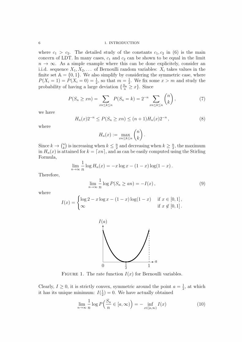
1r
Figure 1. The rate function I(x) for Bernoulli variables.
Clearly, I ≥ 0, it is strictly convex, symmetric around the point a = 12, at which
it has its unique minimum: I(12) = 0. We have actually obtained
limn→∞
1
nlogP
(Sn
n∈ [a,∞)
)
= − infx∈[a,∞)
I(x) (10)
2. LARGE DEVIATIONS 7
By the symmetry of I, we can write
limn→∞
1
nlogP
(∣∣∣Sn
n−m
∣∣∣ ≥ ǫ
)
= − infx:|x−m|≥ǫ
I(x) = −I(ǫ) < 0 . (11)
This is therefore a case where the two constants c1, c2 above can be computedexactly, and shown to be equal. They are expressed in terms of a variationalproblem involving the rate function I.
This result will be generalized to any sequence of i.i.d. random variables in theTheorem of Cramer. Nevertheless, it will not always be possible to obtain I in anexplicit form as above, neither will it be possible to obtain the exact limit (10).The general setup will be the following.
Definition 1.1. A sequence of random variables Z1, Z2, . . . satisfies a Large De-
viation Principle (LDP) if there exists a lower semicontinuous function I : R →[0,∞] with compact level sets such that
(1) for all closed set F ⊂ R,
lim supn→∞
1
nlogP
(
Zn ∈ F)
≤ − infx∈F
I(x) (12)
(2) for all open set G ⊂ R,
lim infn→∞
1
nlogP
(
Zn ∈ G)
≤ − infx∈G
I(x) (13)
It will be seen in the Theorem of Cramer (Section 7 below) that under a finitenesscondition on, Λ, the logarithmic moment generating function of X1, the sequenceSn
nsatisfies a LDP with a rate function given by the Legendre transform of Λ.
A LDP also holds (the Theorem of Gartner-Ellis) in the case where some depen-dence is introduced among the variables Zk, which is a typical situation encoun-tered in statistical mechanics. In that case, the rate function cannot be obtainedby the distribution of a single variable Xi, but through a limiting process equiv-alent to the definition of the free energy/pressure in the thermodynamic limit.
The LDP isn’t restricted to sequences of R-valued random variables, as the se-quence Sn
nabove, but can be defined for more general objects living on more
abstract metric spaces. These appear naturally, even in the study of real i.i.d.sequences. For example, rather than using Sn
nas a macroscopic observable, a finer
description of a large sample is obtained by considering the empirical measureLn ∈ M1(R), defined by
Ln :=1
n
n∑
j=1
δXj,
where δXjis a Dirac mass at Xj. In these terms, the WLLN can be reformulated
by saying that Ln converges weakly to the distribution of X1, ν, in the sensethat
∫f(x)Ln(dx) →
∫f(x)ν(dx) for all bounded continuous function f : R →
R. One can then wonder if some concentration speed for Ln around ν can be
8 1. INTRODUCTION
obtained. Namely, the Theorem of Sanov (see Section) says that Ln also satisfiesa large deviation principle: there exists a convex lower semicontinuous functionI : M1(R) → [0,+∞] such that for all E ⊂ M1(R),
− infµ∈
E
I(µ) ≤ lim infn→∞
1
nlogP
(Ln ∈ E
)
≤ lim supn→∞
1
nlogP
(Ln ∈ E
)≤ − inf
µ∈EI(µ) .
Here, the rate function is in fact given by I(µ) = D(µ|ν), the relative entropyof µ with respect to ν. The above is called a LDP of Level 2. It involves theconvergence of measures on M1(R) and gives a more precise information than thelevel 1. Somehow, the Level 1-LDP should follow from the Level 2-LDP. Namely,since
Sn
n=
∫
xLn(dx) ≡ Φ(Ln) ,
we expect that the concentration of Ln around µ should imply the concentrationof Sn
n= Φ(Ln) around m = Φ(µ). This indeed holds, due to the continuity of the
map Φ : M1(R) → R, as will be seen in the Contraction Principle.
A large part of these notes is to make a close link between the rate functions ofLDT with the thermodynamic potentials of ESM.
3. Spin systems
CHAPTER 2
The Maximum Entropy Principle
As we saw in the introduction, it is more natural to describe a large system ofparticles at equilibrium using a probability distribution, rather than to seek forthe solution of a system of 1025 differential equations. In this section we presenta simple procedure which allows to select this probability measure, in the mostnatural way. The method, called the Maximum Entropy Principle, will selectprobability measures a priori, under certain constraints. Such constraints ap-pear in statistical mechanics, where one studies, for example, systems of particleswhose total energy is fixed. This method is very clearly explained in the papersof Jaynes, [Jay63] and [Jay68]. Later, we use it to introduce the Gibbs distri-bution, the most widely used in equilibrium statistical mechanics.
The technique presented hereafter does not only apply to systems of particles andhas a wide range of applicability. Notice that although it should be consideredas fundamental, the Maximum Entropy Principle will find a justification in thelarge deviation theorems of subsequent chapters.
We start with a simple example. Suppose we are given a dice with 6 faces: throw-ing the dice results in a random number X ∈ 1, 2, . . . , 6. We put ourselves inthe situation where the probabilities pi = P (X = i) are unknown, and our aimis to associate to this dice a suitable probability distribution P = (p1, . . . , p6),pi ≥ 0,
∑6i=1 pi = 1. We are thus assuming that P exists, and our aim is to find it.
Of course, one way of doing, call it empirical, is to throw the dice a large numbern of times, X1, . . . , Xn, and to count the number of times each face appeared: foreach i ∈ 1, 2, . . . , 6,
p(n)i :=
♯1 ≤ k ≤ n : Xk = in
.
Then the Law of Large Numbers guarantees that when n becomes large, the
empirical ratios p(n)i converge to the true values pi:
(p(n)1 , . . . , p
(n)6 ) → (p1, . . . , p6) almost surely.
Unfortunately, we have no time to throw the dice an infinite number of times,and our aim is to find a way of choosing a distribution P a priori to any empiricalmanipulation: our choice must be made taking only into account the informationavailable at hand concerning the dice. It is also important that this association bedone by taking all available information into account. Assuming that our methodleads to a candidate distribution P , the LLN can then be used as a way of testing
9
10 2. THE MAXIMUM ENTROPY PRINCIPLE
if our choice for P matches with the frequencies p(n)i observed experimentally.
In general, the problem of choosing a distribution a priori 1 is under determined:the a priori available information usually doesn’t allow to determine P uniquely.For example, since the dice has six faces and since the constraint
∑6i=1 pi = 1
determines for example p6 in function of the other pis, one would need anotherfive conditions in order to determine P uniquely (if these conditions are not con-tradictory). We are thus faced with the problem of making a choice betweenmany possibilities, and the point is to decide which choice is most natural.
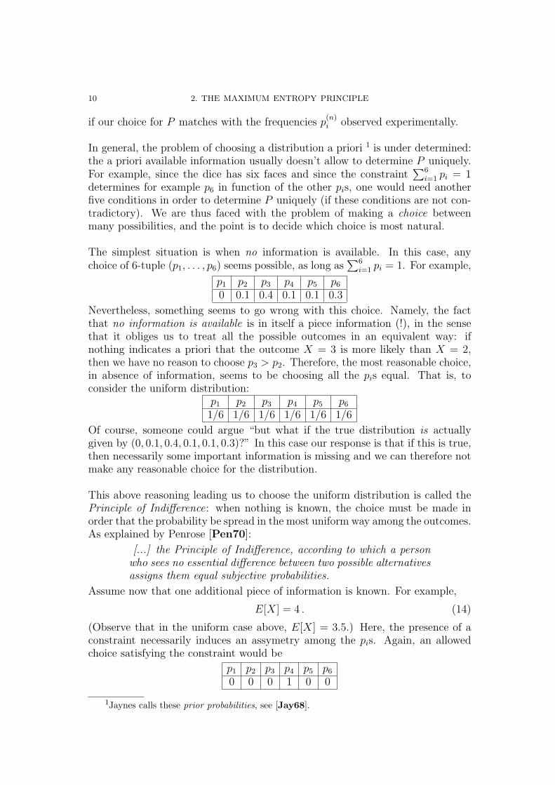
The simplest situation is when no information is available. In this case, anychoice of 6-tuple (p1, . . . , p6) seems possible, as long as
∑6i=1 pi = 1. For example,
p1 p2 p3 p4 p5 p60 0.1 0.4 0.1 0.1 0.3
Nevertheless, something seems to go wrong with this choice. Namely, the factthat no information is available is in itself a piece information (!), in the sensethat it obliges us to treat all the possible outcomes in an equivalent way: ifnothing indicates a priori that the outcome X = 3 is more likely than X = 2,then we have no reason to choose p3 > p2. Therefore, the most reasonable choice,in absence of information, seems to be choosing all the pis equal. That is, toconsider the uniform distribution:
p1 p2 p3 p4 p5 p61/6 1/6 1/6 1/6 1/6 1/6
Of course, someone could argue “but what if the true distribution is actuallygiven by (0, 0.1, 0.4, 0.1, 0.1, 0.3)?” In this case our response is that if this is true,then necessarily some important information is missing and we can therefore notmake any reasonable choice for the distribution.
This above reasoning leading us to choose the uniform distribution is called thePrinciple of Indifference: when nothing is known, the choice must be made inorder that the probability be spread in the most uniform way among the outcomes.As explained by Penrose [Pen70]:
[...] the Principle of Indifference, according to which a personwho sees no essential difference between two possible alternativesassigns them equal subjective probabilities.
Assume now that one additional piece of information is known. For example,
E[X] = 4 . (14)
(Observe that in the uniform case above, E[X] = 3.5.) Here, the presence of aconstraint necessarily induces an assymetry among the pis. Again, an allowedchoice satisfying the constraint would be
p1 p2 p3 p4 p5 p60 0 0 1 0 0
1Jaynes calls these prior probabilities, see [Jay68].
2. THE MAXIMUM ENTROPY PRINCIPLE 11
but again, this choice seems to favorize overwhelmingly the outcome X = 4.Rather, one needs to apply something analogous to the Principle of Indifferenceamong the set of distributions that satisfy (14). Since the distribution we arelooking for is obviously non-uniform, it is not clear how exactly this principleshould be applied: the distribution we are looking for must satisfy (14) and beat the same time “closest” to the uniform distribution. Ideally, one needs to seekfor a function quantifying the spread of a distribution, which should be maximalwhen the distribution is uniform.
It might be surprising to learn that there is essentially a unique way of defin-ing this function, introduced by Shannon in 1948. This function associates to(p1, . . . , pk) a number H = H(p1, . . . , pk) called entropy. H has many interpreta-tions, but its main feature is that it allows to measure, in some sense (which willbe made clearer when introducing relative entropy), the distance to the uniformdistribution. The spread of a distribution is larger when the distribution is closeto uniform. This can be expressed by saying that the spreading of the distributionturns the outcome of a realization more uncertain. Entropy therefore providesa way of measuring our uncertainty with respect to the outcome of a randomexperiment. Citing again Jaynes [Jay63],
Our problem is to find a probability assignment which avoidsbias, while agreeing with whatever information is given. [...]The great advance provided by Information Theory lies in thediscovery that there is a unique, unambiguous criterion for theamount of uncertainty represented by a discrete probability dis-tribution, which agrees with our intuition that a broad distri-bution represents more uncertainty than does a sharply peakedone.
The following definition of entropy was given by C.E. Shannon in [Sha48].
Definition 2.1. The entropy of a probability distribution (p1, . . . , pk) is definedby
H(p1, p2, . . . , pk) := −k∑
j=1
pj log pj , (15)
where it is assumed that the logarithm is with respect to the base e, and where wemake the convention that 0 log 0 := 0.
Let us verify that this definition suits our requirements for a function measuringour ignorance with respect to the outcome of the random experiment. First, ob-serve that H is a positive quantity which attains its minimal value H = 0 exactlywhen all but one pis are zero, and the last one equals 1. In any of these cases,the outcome of the experiment is certain, and so the uncertainty must be zero.
Then, we show that entropy is maximal for the uniform distribution:
H(p1, . . . , pk) ≤ H(1k, . . . , 1
k
)= log k . (16)
12 2. THE MAXIMUM ENTROPY PRINCIPLE
Namely, consider the strictly concave function ψ(x) := −x log x for x ∈ (0, 1],ψ(0) := 0. We have
H(p1, . . . , pk) =k∑
j=1
ψ(pj) = kk∑
j=1
1kψ(pj)
≤ kψ( 1k) = log k = H
(1k, . . . , 1
k
).
Therefore, (16) fullfills our previous requirement: the uncertainty with respectto the outcome of the experience is maximal when the distribution is uniform..Moreover, in Shannon’s own words, any change towards equalization of the prob-abilities (p1, . . . , pk) increases H(p1, . . . , pk). This can be seen by explicit calcu-lation, by considering the variation of H when, say p1(s) = p0+ s, p2(s) = p0− s,with sց 0, and where the other k − 2 variables are kept fixed:
d
dsH =
d
ds
[− (p0 + s) log(p0 + s)− (p0 − s) log(p0 − s)
]
= logp0 − s
p0 + s,
which is < 0 when s > 0. This means that if s decreases, i.e. when p1 and p2tend to equalize, then the entropy increases.
A further property of H is that it is a concave function of p = (p1, . . . , pk).To gain geometric intuition, we can identify the set of probability distributions(p1, . . . , pk) with the simplex
M1 :=
p =k∑
j=1
pjej : pj ≥ 0,k∑
j=1
pj = 1
⊂ Rk .
Any p ∈ M1 can thus be considered as a convex combination of the extremeelements ofM1, which are the unit vectors of the canonical basis of Rk: e1, . . . , ek.At each extreme element ej, H(ej) = 0. By the concavity of ψ, for any p1,p2 ∈M1, 0 ≤ λ ≤ 1,
H(λp1 + (1− λ)p2) ≥ λH(p1) + (1− λ)H(p2) .
One thus has a picture of H as a concave function on M1 which attains its max-imum (log k) at the barycenter of M1, namely ( 1
k, . . . , 1
k).
Going back to our problem of selecting a probability distribution under a con-straint, (Jaynes [Jay63])
In making inference on the basis of partial information we mustuse that probability distribution which has the maximum entropysubject to whatever is known. This is the only unbiased assign-ment we can make; to use any other would amount to arbitraryassumption of information, which by hypothesis we don’t have.
Consider the dice problem. Following Jaynes, the proper unbiased probabilitydistribution is the one that maximises H(p1, . . . , p6), with possible additional
1. THE GIBBS DISTRIBUTION 13
constraints. When no constraint is fixed (other than (p1, . . . , p6) being a proba-bility), the problem then reduces to
Maximise H(p1, . . . , p6) over M1.
As we have seen, the unique solution to this problem is the uniform probability(16, . . . , 1
6). Now if one imposes that E[X] = 4, then with M′
1 := (p1, . . . , p6) ∈M1 :
∑6j=1 jpj = 4, the problems becomes:
Maximise H(p1, . . . , p6) over M′1.
This optimization problem can be solved using the method of Lagrange multipli-ers. Since there are two constraints, we introduce two Lagrange multipliers λ, β,and define
L(p1, . . . , p6) := H(p1, . . . , p6)− λ6∑
i=1
pi − β6∑
i=1
ipi .
The optimization problem then turns into the analytic resolution of the system
∇L = 0 ,∑6
i=1 pi = 1 ,∑6
i=1 ipi = 4 .
As can be easily verified using the Lagrange multipliers , the solution of thisproblem is given by
pi =e−β∗i
Z(β∗),
where
Z(β) =6∑
i=1
e−βi ,
and where β∗ denotes the unique solution of
− d
dβlogZ(β) = 4 .
The solution (p1, . . . , p6) is therefore the solution of the variational problem
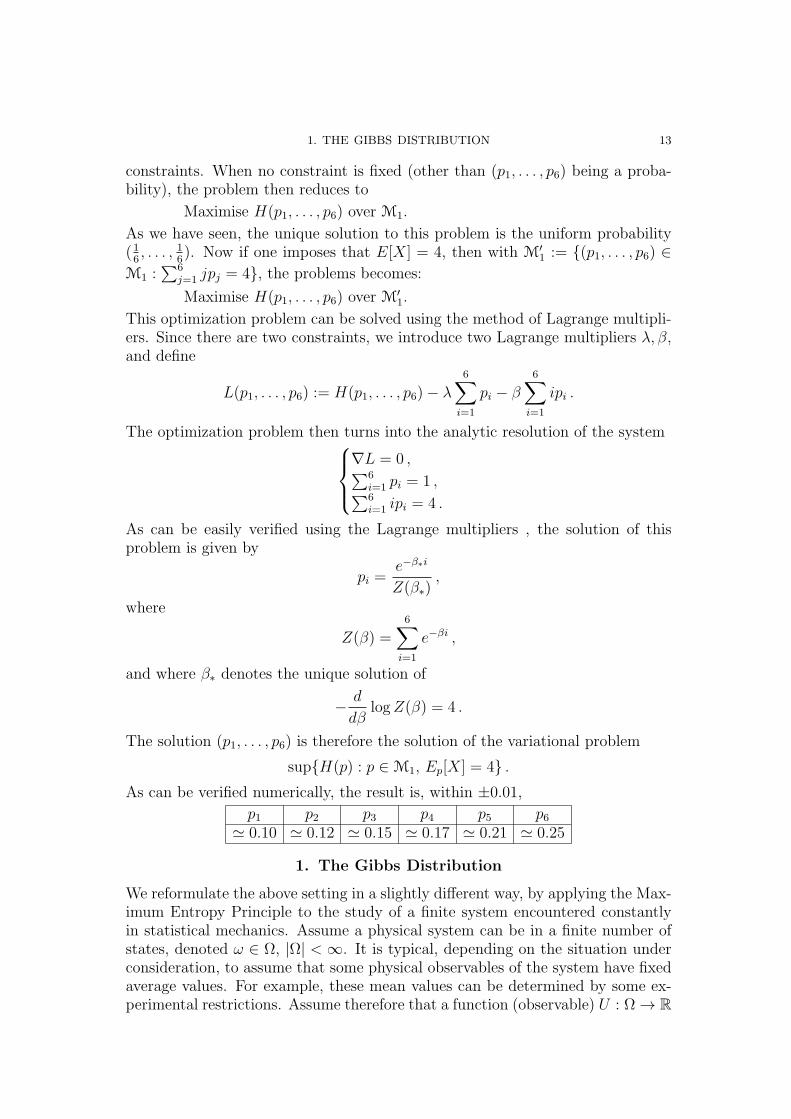
supH(p) : p ∈ M1, Ep[X] = 4 .As can be verified numerically, the result is, within ±0.01,
p1 p2 p3 p4 p5 p6≃ 0.10 ≃ 0.12 ≃ 0.15 ≃ 0.17 ≃ 0.21 ≃ 0.25
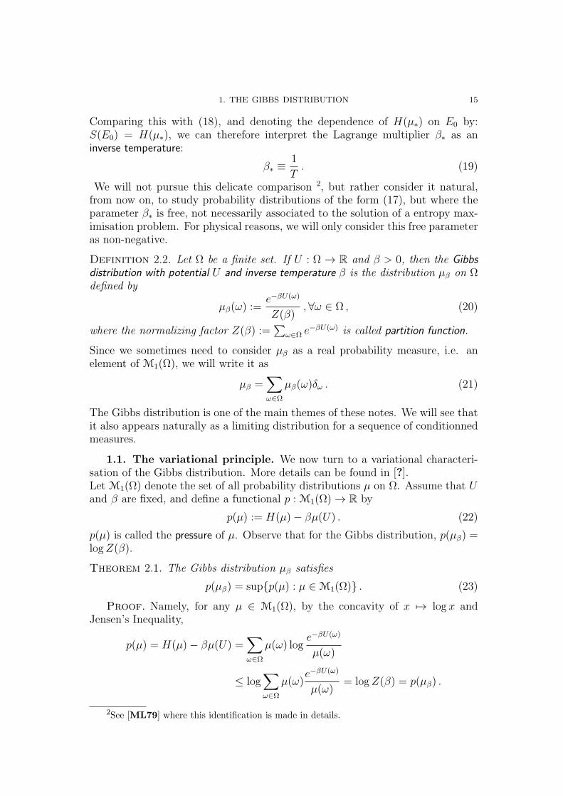
1. The Gibbs Distribution
We reformulate the above setting in a slightly different way, by applying the Max-imum Entropy Principle to the study of a finite system encountered constantlyin statistical mechanics. Assume a physical system can be in a finite number ofstates, denoted ω ∈ Ω, |Ω| < ∞. It is typical, depending on the situation underconsideration, to assume that some physical observables of the system have fixedaverage values. For example, these mean values can be determined by some ex-perimental restrictions. Assume therefore that a function (observable) U : Ω → R
14 2. THE MAXIMUM ENTROPY PRINCIPLE
is given. Although it is arbitrary, in most cases U(ω) represents the energy ofthe microscopic state ω. If no other information is given , what is the most nat-ural (or “least biased”) probability distribution µ = (µ(ω), ω ∈ Ω), satisfying theconstraint that Eµ[U ] = E0? (Here, E0 ∈ (minU,maxU).) As before, the Max-imum Entropy Principle leads to the following optimisation problem: maximisethe Shannon Entropy
H(µ) = −∑
ω∈Ω
µ(ω) log µ(ω) ,
under the constraints
µ(ω) ≥ 0,∑
ω∈Ω
µ(ω) = 1 ,∑
ω∈Ω
µ(ω)U(ω) = E0 .
As we saw, by a direct application of the method of the Lagrange multipliers, thesolution is obtained by first finding the Lagrange multiplier β∗ = β∗(E0), solutionof
− d
dβlogZ(β) = E0 ,
where Z(β) is the partition function, defined by
Z(β) :=∑
ω∈Ω
e−βU(ω) .
(As can be verified, β∗ exists as soon as E0 ∈ (minU,maxU).) Then, the max-imiser µ∗ = (µ∗(ω), ω ∈ Ω) of the Shannon Entropy is given by
µ∗(ω) =e−β∗U(ω)
Z(β∗), ∀ω ∈ Ω . (17)
The measure µ∗ has thus been constructed so that Eµ∗[U ] = E0, and its Shannon
Entropy is maximal among all measures µ satisfying this condition. By a directcomputation,
H(µ∗) = β∗Eµ∗[U ] + logZ(β∗) = β∗E0 + logZ(β∗) .
Therefore,
∂H
∂E0
= E0∂β∗∂E0
+ β∗ +∂
∂E0
logZ(β∗)
= E0∂β∗∂E0
+ β∗ +∂
∂βlogZ(β)
∣∣∣β=β∗
︸ ︷︷ ︸
=−E0
∂β∗∂E0
= β∗ . (18)
Assume for a while that U(ω) is the energy of the state ω. Then we can comparethis last display with the fundamental thermodynamic relation between entropyS, internal energy E and temperature T :
∂S
∂E=
1
T.
1. THE GIBBS DISTRIBUTION 15
Comparing this with (18), and denoting the dependence of H(µ∗) on E0 by:S(E0) = H(µ∗), we can therefore interpret the Lagrange multiplier β∗ as aninverse temperature:
β∗ ≡1
T. (19)
We will not pursue this delicate comparison 2, but rather consider it natural,from now on, to study probability distributions of the form (17), but where theparameter β∗ is free, not necessarily associated to the solution of a entropy max-imisation problem. For physical reasons, we will only consider this free parameteras non-negative.
Definition 2.2. Let Ω be a finite set. If U : Ω → R and β > 0, then the Gibbs
distribution with potential U and inverse temperature β is the distribution µβ on Ωdefined by
µβ(ω) :=e−βU(ω)
Z(β), ∀ω ∈ Ω , (20)
where the normalizing factor Z(β) :=∑
ω∈Ω e−βU(ω) is called partition function.
Since we sometimes need to consider µβ as a real probability measure, i.e. anelement of M1(Ω), we will write it as
µβ =∑
ω∈Ω
µβ(ω)δω . (21)
The Gibbs distribution is one of the main themes of these notes. We will see thatit also appears naturally as a limiting distribution for a sequence of conditionnedmeasures.
1.1. The variational principle. We now turn to a variational characteri-sation of the Gibbs distribution. More details can be found in [?].Let M1(Ω) denote the set of all probability distributions µ on Ω. Assume that Uand β are fixed, and define a functional p : M1(Ω) → R by
p(µ) := H(µ)− βµ(U) . (22)
p(µ) is called the pressure of µ. Observe that for the Gibbs distribution, p(µβ) =logZ(β).
Theorem 2.1. The Gibbs distribution µβ satisfies
p(µβ) = supp(µ) : µ ∈ M1(Ω) . (23)
Proof. Namely, for any µ ∈ M1(Ω), by the concavity of x 7→ log x andJensen’s Inequality,
p(µ) = H(µ)− βµ(U) =∑
ω∈Ω
µ(ω) loge−βU(ω)
µ(ω)
≤ log∑
ω∈Ω
µ(ω)e−βU(ω)
µ(ω)= logZ(β) = p(µβ) .
2See [ML79] where this identification is made in details.
16 2. THE MAXIMUM ENTROPY PRINCIPLE
We will move back to the variational principle when describing the contractionprinciple for LDPs of level 3.
2. Uniqueness of Entropy
In this section, following Khinchin [Khi57], we show that the entropy H de-fined in (15) is the unique function satisfying a set of natural conditions that aresuggested by the intuitive notion of uncertainty about the outcome of a randomexperience, or its unpredictability.
It is useful to formulate the problem in a slightly more general manner. Considera random experiment modelized by some probability space (Ω,F, P ). A finitescheme is a partition A of Ω into a finite number of sets Ak ∈ F (called atoms)together with their associated probabilities pk := P (Ak). Altough we will usu-ally denote a scheme by A = (A1, . . . , An), it should always be remembered thatthe probabilities (P (A1), . . . , P (An)) are part of the information contained in A.A scheme can represent a simple experiment, like the throw of a dice (whereAk = the kth face shows up), but it can also modelize the coarse-grainingof a more complicated experiment where instead of the true result of the ran-dom experiment, i.e. ω, one is interested in the atom Ak of the partition A towhich ω belongs. The coarse-grained result of the experience is therefore an indexk = k(ω) ∈ 1, 2, . . . , n, giving the unique atom Ak ∋ ω, and can be consideredas partial knowledge about the result of the experiment.
How can one define the unpredictability of a random experience modelized by afinite scheme A = (A1, . . . , An)? The unpredictability of A can of course dependonly on the probabilities (P (A1), . . . , P (An)). That is, we are looking for a classof functions
H(A) = H(P (A1), . . . , P (An)) .
We will define four conditions (see (I)-(IV) below) that H should satisfy, most ofwhich will be natural in terms of unpredictability 3, and then show that these leadunambiguously to the only possibility H = HSh (up to a multiplicative constant),where according to Definition 2.1, the Shannon Entropy HSh is defined by
HSh(A) = −∑
A∈A
P (A) logP (A) . (24)
A first condition we should impose is that the unpredictability of a random ex-perience be continuous in its arguments:
H is continuous. (I)
Next, as we have seen for HSh, we need that unpredictability be maximal whenthe distribution is uniform. Let us call a scheme uniform when its atoms have
3The only exception being maybe (IV), which has to do with extensivity; this conditionseems natural to me although I understand some might find it completely arbitrary.
2. UNIQUENESS OF ENTROPY 17
equal probabilities. The second requirement we impose on H is therefore that
H is maximal on uniform schemes. (II)
To state the third requirement, we introduce a few notations. Consider twoschemes, say A = (A1, . . . , Ak) and B = (B1, . . . , Bk), giving a coarse-graineddescription of the same random experiment. Consider the composite scheme A∨Bdefined by
A ∨B := A ∩ B : A ∈ A, B ∈ B .This scheme is a refinement of both A and B, since each of its atoms containsa double information (ω ∈ A and ω ∈ B for some couple (A,B)). It is easy tosee that when A and B are independent, that is if P (A∩B) = P (A)P (B) for allpair A ∈ A, B ∈ B, then
HSh(A ∨B) = HSh(A) +HSh(B) . (25)
This property is called extensivity. In the general case (i.e. without assumingindependence) we always have
HSh(A ∨B) ≥ −∑
(A,B)
P (A ∩B) logP (A) = HSh(A) .
The exact excess in the previous inequality,
HSh(B|A) := HSh(A ∨B)−HSh(A) , (26)
measures the average excess of information produced by the outcome of the ex-periment A ∨ B over the information produced by the experiment A. For anyevent A, P (A) > 0, define
HSh(B|A) := −∑
B∈B
P (B|A) logP (B|A) .
As can be verified explicitely,
HSh(B|A) =∑
A∈A
P (A)HSh(B|A) . (27)
The above quantities can be defined in general for finite schemes:
H(B|A) := H(P (B1|A), . . . , P (Bk|A)) ,and
H(B|A) :=∑
A∈A
P (A)H(B|A) .
A fundamental property that should be satisfied by entropy is therefore that
H(A ∨B) = H(A) +H(B|A) . (III)
The interpretation of this identity in terms of unpredictability is clear. The finalcondition says that unpredictability is not affected by the presence of atoms whoseprobability is zero:
If A = (A1, . . . , Ak) with P (Ak) = 0, and A′ = (A1, . . . , Ak−2, A′k−1),
where A′k−1 = Ak−1 ∪ Ak, then H(A) = H(A′). (IV)
18 2. THE MAXIMUM ENTROPY PRINCIPLE
Theorem 2.2. Let H be a function defined on probability distributions of finiteschemes, such that (I)-(IV) hold. Then H = HSh, up to a positive constant.
We first prove Theorem 2.2 for uniform schemes, which leads to (28), the Entropyof Boltzmann in its simplest form. If U is a scheme, |U| denotes the number ofelements of its partition.
Lemma 2.1. Let H be a function defined on uniform finite schemes which ismonotone increasing in |U|, and which is extensive, in the sense that if U, U′ aretwo independent uniform schemes, then
H(U ∨ U′) = H(U) +H(U′) .
Then there exists a constant λ > 0 such that for all uniform scheme U,
H(U) = λ log |U| . (28)
Proof. Let L(k) denote the value of H on schemes of size k. By the firstassumption, L(k) is non-decreasing. Let U1, . . . ,Um be independent, containingeach r elements. On one hand, by extensivity,
H(U1 ∨ · · · ∨ Um) =m∑
j=1
H(Uj) = mL(r).
On the other hand, U1 ∨ · · · ∨ Um is also uniform and contains rm elements.Therefore, H(U1∨· · ·∨Um) = L(rm). This shows that L(rm) = mL(r). We thencheck that the logarithm is the unique function satisfying this condition for allm ≥ 1, r ≥ 1. Namely, fix any s ≥ 1, n ≥ 1 and find some m ≥ 1 such thatrm ≤ sn < rm+1. Therefore, m log r ≤ n log s < (m + 1) log r, and since L ismonotone and L(sn) = nL(s), we have
m
n≤ L(s)
L(r)≤ m+ 1
n.
Altogether, these imply that∣∣∣L(s)
L(r)− log s
log r
∣∣∣ ≤ 1
n.
Since n was arbitrary, this shows that there exists λ such that L(r) = λ log r. λmust be positive in order for L to be monotone increasing.
Proof of Theorem 2.2: Assume H satisfies (I)-(IV). For a while, let Hk
denote the function associated to schemes with k elements. Then clearly
Hk(1k, . . . , 1
k)(IV)= Hk+1(
1k, . . . , 1
k, 0)
(II)
≤ Hk+1(1
k+1, . . . , 1
k+1, 1k+1
) ,
which implies that for uniform schemes, H is increasing of the number of elements.By (III), H is of course extensive for independent partitions. H therefore satisfiesthe conditions of the lemma, and so H(U) = λ log |U| for all uniform scheme.Let then A = (A1, . . . , An) be a scheme with rational probabilities pk (the exten-sion to arbitrary probabilities pk then follows by the continuity hypothesis (I)).That is, pk = wk
W, where wk ∈ N and W =
∑n
k=1wk. It is useful to reinterpretthe probabilities as follows. Consider a set of W balls numbered from 1 to W ,
2. UNIQUENESS OF ENTROPY 19
w1 of which are painted with a color c1, w2 of which are painted with a colorc2, etc. (we assume all the colors are different). A ball is drawn at random,uniformly. Then if we define A′
j as the even “the ball drawn has color cj”, then
P (A′j) =
ωj
W≡ P (Aj). Therefore, H(A) = H(A′), where A′ = (A′
1, . . . , A′n). Let
B = (B1, . . . , BW ) be made of the smallest possible atoms of the experience: Bi
is the event “the ball i was drawn”. Then clearly,
P (Bi|A′j) =
1wj
if i ∈ A′j
0 otherwise.
By the lemma, H(B|A′j) = λ logwj. Therefore,
H(B|A′) =n∑
j=1
pjH(B|A′j) = λ
n∑
j=1
pj log pj + λ logW
But since A′∨B contains events of equal probabilities (W of which are non-zero),we have again by (IV) and the lemma that H(A′ ∨ B) = λ logW . Therefore, byassumption (III),
H(A′) = H(A′ ∨B)−H(B|A′) = −λn∑
j=1
pj log pj .
Since H(A) = H(A′), this finishes the proof.

CHAPTER 3
Large Deviations for finite alphabets
In this chapter, we expose large deviation result for i.i.d. sequences X1, X2, . . .taking values in a finite set. The advantage of working with finite alphabets isthat it allows to rely on combinatorial rather than analytical methods, and al-ready gives a framework in which many interesting statistical mechanical systemscan be studied, for example the ideal gas of the next section. On the other hand,the results obtained are already far-reaching, and illustrate the main conceptsthat will be encountered later in more general settings.
This chapter will contain two kinds of results: first, those describing the concen-tration properties of the empirical mean Sn
n, called Level-1 LDPs. Second, those
describing the concentration of the empirical measure Ln, called Level-2 LDPs.
1. The Theorem of Sanov
Note that in the case where the variables Xj are Bernoulli, i.e. taking values inthe alphabet A = 0, 1, we have obtained in (10), Chapter 1, a precise asymp-totic behaviour of the frequency of 1s, i.e. Sn
n. Since the alphabet contains only
two letters, this of course automatically gives the frequency of 0s, equal to 1− Sn
n.
The LLN thus implies that the empirical measure (Sn
n, 1 − Sn
n), which give the
frequency of each symbol in a sample of size n, converges to its theoretical value(12, 12), exponentially fast with n. In the general case, where the alphabet can
contain more than two letters, the combinatorics is a little more complicated, buta similar result holds, known as the Theorem of Sanov.
In this section, we study a more general situation, in which the random variablesXj take values in a finite alphabet A. Let M1 = M1(A) denote the set of allprobabilty distributions on A, which we identify with the vectors µ = (µ(a), a ∈A) with µ(a) ≥ 0,
∑
a∈A µ(a) = 1. We equip M1 with the L1-metric, (also calledtotal variation distance), defined by
‖µ− ν‖1 :=∑
a∈A
|µ(a)− ν(a)| .
Teh interior of a set E ⊂ M1 is denoted intE, and its closure E. We will denotethe common distribution of the Xjs by ν: ν(a) := P (Xj = a). Without loss ofgenerality, we can assume that ν(a) > 0 for all a ∈ A. We also assume that the se-quence X1, X2, . . . is constructed canonically on the sequence space AN, endowedwith the σ-algebra generated by cylinders, and denote the product measure on
21
22 3. LARGE DEVIATIONS FOR FINITE ALPHABETS
this space by Pν .
Rather than just Sn
n, we study the frequency of appearance of each of the symbols
of the alphabet up to time n. Therefore, the empirical measure associated to afinite sample X1, . . . , Xn, is the probability distribution Ln ∈ M1 defined by
Ln :=1
n
n∑
j=1
δXj.
Ln is also called the type of the sample X1, . . . , Xn. In terms of Ln, the Lawof Large Numbers takes the following form: if ν ∈ M1 denotes the commondistribution of the Xis, then
Ln ⇒ ν , Pν-almost surely (29)
where ⇒ denotes weak convergence, which in the case of a finite alphabet reducesto ‖Ln − ν‖1 → 0.
The Theorem of Sanov describes the exponential concentration of Ln in thevincinity of ν. The cost of the empirical measure being far from ν will be mea-sured with the following function.
Definition 3.1. Let µ and ν be two probability distributions on A. The relative
entropy of µ with respect to ν, is defined by
D(µ‖ν) :=∑
a∈A
µ(a) logµ(a)
ν(a).
Our convention is that 0 log 0 := 0, and 0 log 0 := 00.
D is also called Kullback-Leibler distance, or information divergence between µ andν. Observe that if µ is not absolutely continuous with respect to ν (i.e. if thereexists a ∈ A such that µ(a) > 0, ν(a) = 0), then D(µ‖ν) = +∞. We list a fewproperties of D(·‖·).Proposition 3.1. Assume ν > 0. D satisfies the following properties:
(1) D(µ‖ν) ≥ 0, with equality if and only if µ = ν,(2) µ 7→ D(µ‖ν) is strictly convex and continuous on M1,(3) (µ, ν) 7→ D(µ‖ν) is convex.Proof. Write, temporarily,
D(µ‖ν) =∑
a∈A
ν(a)ψ(µ(a)
ν(a)
)
,
where ψ is the strictly convex function ψ(x) = x log x. Jensen’s inequality givesD(µ‖ν) ≥ ψ(1) = 0, with equality if and only if µ(a)/ν(a) = 1 for all a ∈ A, thusproving (1). For (2), the strict convexity and continuity ofD(·|ν) follow by that ofψ. For (3), we use the following (called log-concave inequality): if a1, . . . , an ≥ 0,b1, . . . , bn ≥ 0,
n∑
j=1
aj logajbj
≥( n∑
j=1
aj
)
log
∑n
j=1 aj∑n
j=1 bj,
1. THE THEOREM OF SANOV 23
with equality if and only if there exists a constant c such that aj = cbj for all j.Therefore if (µ′, ν ′) =
∑n
i=1 λi(µi, νi) with∑n
i=1 λi = 1, we have
D(µ′‖ν ′) =∑
a∈A
( n∑
i=1
λiµi(a))
log
∑n
i=1 λiµi(a)∑n
i=1 λiνi(a)
≤∑
a∈A
n∑
i=1
λiµi(a) logλiµi(a)
λiνi(a)
=n∑
i=1
λiD(µi‖νi) ,
with equality if and only if µi = νi for all i.
Although these properties remind those of a distance, D is actually not a distance:it is not symetric in general, as can be seen by constructing a simple example onan alphabet with two letters. Nevertheless, we have a usefull comparison withthe total variation distance:
Proposition 3.2 (Pinsker’s Inequality). For all µ, ν ∈ M1,
D(µ‖ν) ≥ 1
2‖µ− ν‖21 (30)
Therefore, if µ and ν are close in the sense of D(·‖·), they are also close in thesense of ‖ · ‖TV.
Observe that if ν is the uniform distribution, ν(a) = 1/|A|, thenD(µ‖ν) = log |A| −H(µ) . (31)
Then (2) implies that µ→ H(µ) is concave, as we already knew, but also that inthis case, D measures the same discrepancy as the Shannon Entropy does withrespect to the uniform distribution. Relative entropy can be thus be considered asa generalization of the Shannon Entropy to the case where the reference measureis ν rather than the uniform distribution.
We now state the theorem.
Theorem 3.1 (Theorem of Sanov). Let X1, X2, . . . be i.i.d. with common distri-bution ν. For all E ⊂ M1,
Pν(Ln ∈ E) ≤ (n+ 1)|A| exp(−n inf
µ∈ED(µ‖ν)
). (32)
Moreover,
− infµ∈intE
D(µ‖ν) ≤ lim infn→∞
1
nlogPν(Ln ∈ E) (33)
≤ lim supn→∞
1
nlogPν(Ln ∈ E) ≤ − inf
µ∈ED(µ‖ν) . (34)
24 3. LARGE DEVIATIONS FOR FINITE ALPHABETS
Remark 3.1. A particular feature of the upper bound (34) is that it does notimpose any restriction on the set E. Nevertheless, if E is open, or more generally,if E ⊂ intE (this forbids E to have isolated points, in particular), then
infµ∈intE
D(µ‖ν) ≥ infµ∈E
D(µ‖ν) ≥ infµ∈intE
D(µ‖ν) = infµ∈intE
D(µ‖ν)
The last equality follows from the continuity of D(·‖ν). Therefore the two boundsin the theorem coincide, and:
limn→∞
1
nlogPν(Ln ∈ E) = − inf
µ∈ED(µ‖ν) .
For later reference, we say that the open sets have theD(·‖ν)-continuity property.
The proof of Theorem 3.5 relies on simple combinatorial arguments. Denote byLn the set of all possible types of sequences of size n. For example, if |A| = 2,Ln = (0, 1), ( 1
n, n−1
n), . . . , (n−1
n, 1n), (1, 0).
Lemma 3.1. |Ln| ≤ (n+ 1)|A|.
Proof. Each L ∈ Ln can be identified with an n-tuple (l1, . . . , l|A|), withlj ∈ 0, 1, 2, . . . , n,
∑
j lj = n. But without this last constraint, the number of
such n-tuples is exactly (n+ 1)|A|.
If x = (x1, . . . , xn) ∈ An, we denote its type by Lx, and write Pν(x) := Pν(X1 =
x1, . . . , Xn = xn).
Lemma 3.2. For all x ∈ An, Pν(x) depends only on the type of x, and
Pν(x) = exp[−n(H(Lx) +D(Lx‖ν))
]. (35)
(35) nicely expresses the fact that D(Lx‖ν) represents the cost of Lx being dif-ferent from ν.
Proof. First, H(Lx) + D(Lx‖ν) = −∑
a∈A Lx(a) log ν(a). Then, by inde-pendence,
Pν(x) =n∏
i=1
ν(xi) =∏
a∈A
ν(a)|i≤n:xi=a|
=∏
a∈A
ν(a)nLx(a) = en∑
a∈ALx(a) log ν(a) ,
which gives (35).
If µ ∈ Ln, we denote the type class of µ as An(µ) := x ∈ An : Lx = µ. We have
|An| = |A|n = en log |A|, but
Lemma 3.3. For all type µ ∈ Ln,
(n+ 1)−|A|enH(µ) ≤ |An(µ)| ≤ enH(µ) . (36)
Since the Shannon Entropy is maximal for the uniform distribution, (36) saysthat the uniform distribution also has the largest type class.
1. THE THEOREM OF SANOV 25
Proof. For the upper bound, we use Lemma 3.2:
1 ≥ Pµ(An(µ)) =
∑
x∈An(µ)
e−nH(µ) = |An(µ)|e−nH(µ) .
For the lower bound, we use Lemma 3.1:
1 =∑
µ′∈Ln
Pµ(An(µ′)) ≤ |Ln| max
µ′∈Ln
Pµ(An(µ′)) .
We claim that maxµ′∈LnPµ(A
n(µ′)) ≤ Pµ(An(µ)), which will give the lower bound
since Pµ(An(µ)) = |An(µ)|e−nH(µ), as already seen.
Pµ(An(µ))
Pµ(An(µ′))=
|An(µ)|∏
a∈A µ(a)N(a)
|An(µ′)|∏a∈A µ(a)N ′(a)
,
whereN(a) = nµ(a), N ′(a) = nµ′(a). Since, by a simple combinatorial argument,
|An(µ)| = n!∏
a∈AN(a)!,
we havePµ(A
n(µ))
Pµ(An(µ′))=
∏
a∈A
N ′(a)!
N(a)!µ(a)N(a)−N ′(a)
Since m!n!
≥ nm−n for all m,n, this product is bounded below by∏
a∈A
N(a)N′(a)−N(a)µ(a)N(a)−N ′(a) =
∏
a∈A
nN ′(a)−N(a) = 1 ,
since∑
a∈A
(N ′(a)−N(a)
)= n
∑
a∈A
(µ′(a)− µ(a)
)= n− n = 0.
Proposition 3.3. Let ν ∈ M1. For any µ ∈ Ln,
(n+ 1)−|A|e−nD(µ‖ν) ≤ Pν(An(µ)) ≤ e−nD(µ‖ν) . (37)
Proof. The proof follows by using Lemma 3.2,
Pν(An(µ)) =
∑
x∈An(µ)
Pν(x) = |An(µ)| exp[−n(H(µ) +D(µ‖ν))
],
and by using Lemma 3.3 to estimate |An(µ)|.
Proof of Theorem 3.5: The upper bound (32) (from which (34) followsimmediately) is obtained as follows:
Pν(Ln ∈ E) =∑
µ∈E∩Ln
Pν(An(µ)) (38)
by Proposition 3.3 ≤∑
µ∈E∩Ln
e−nD(µ‖ν)
≤ |Ln|e−n infµ∈E D(µ‖ν) ,
26 3. LARGE DEVIATIONS FOR FINITE ALPHABETS
and |Ln| is estimated using Lemma 3.1. For the lower bound (33),
Pν(Ln ∈ E) =∑
µ∈E∩Ln
Pν(An(µ))
≥ (n+ 1)−|A| supµ∈E∩Ln
e−nD(µ‖ν) ,
where we used Proposition 3.3. Therefore,
lim infn→∞
1
nlogPν(Ln ∈ E) ≥ − lim sup
n→∞inf
µ∈E∩Ln
D(µ‖ν) .
Let µ0 ∈ intE. Then clearly, there exists a sequence µn ∈ E ∩ Ln such that‖µn − µ0‖1 → 0. Therefore,
lim supn→∞
infµ∈E∩Ln
D(µ‖ν) ≤ lim supn→∞
D(µn‖ν) = D(µ0‖ν) ,
by the continuity of D (Proposition 3.1). This gives (33).
As we have seen, when ν is the uniform distribution, D(µ‖ν) = log |A| −H(µ).Therefore, if E ⊂ M1, we have
infµ∈E
D(µ‖ν) = log |A| − supµ∈E
H(µ) .
The variational problem that appears in the Sanov estimates is thus related, inthis case, to a maximization of the Shannon Entropy. We will come back to thislater.
1.1. The Theorem of Sanov, General Case. The Theorem of Sanovis general and holds when the random variables Xj take values in a completeseparable metric space S 1. Without proof, we will state this theorem in thesimple case where S = R. The first step towards this generalization is to redefinethe relative entropy.
Definition 3.2. Let µ, ν ∈ M1(R) be two probability measures on R. The relativeentropy of µ with respect to ν is defined by
D(µ‖ν) :=∫
f log f dν if µ≪ ν, and f = dµ
dν,
+∞ otherwise.(39)
As before, it can be shown that µ → D(µ‖ν) is convex. We equip M1(R) withthe topology of weak convergence. That is, say that a sequence µn converges toµ if
∫
f dµn →∫
f dµ
for all continuous bounded function f : R → R. It can be shown that with respectto the weak topology, µ→ D(µ‖ν) is lower semicontinuous and has compact levelsets.
1This happens to be a corollary of an even more general result, the Theorem of Cramer ininfinite dimensional spaces. See [OV05].
2. APPLICATIONS 27
Theorem 3.2 (Theorem of Sanov). Let X1, X2, . . . be i.i.d. with common distri-bution ν ∈ M1(R).
(1) For all closed set C ⊂ M1(R),
lim supn→∞
1
nlogPν(Ln ∈ C) ≤ − inf
µ∈CD(µ‖ν) . (40)
(2) For all open set G ⊂ M1(R),
lim infn→∞
1
nlogPν(Ln ∈ G) ≥ − inf
µ∈GD(µ‖ν) (41)
Proof. See [OV05], p.58.
2. Applications
We go back to the case of a finite alphabet. Since the Theorem of Sanov 3.5gives precise information on the convergence of the empirical measure Ln, itseems natural to ask whether it allows to derive similar informations about theempirical mean Sn
n. Let us be a little more general, and consider partial sums of
the form Sfn := f(X1) + · · · + f(Xn), where f : A → R, and where as before the
Xis are i.i.d., A-valued with distribution ν. We introduce the notation
〈f, µ〉 :=∫
A
f dµ =∑
a∈A
µ(a)f(a) ,
with which Sfn
n= 〈f, Ln〉. Therefore, for A ⊂ R
Sfn
n∈ A⇔ Ln ∈ E
fA (42)
where EfA := µ ∈ M1 : 〈f, µ〉 ∈ A. Using this observation, we give two
applications of the Theorem of Sanov.
2.1. The Law of Large Numbers. Here we assume that A ⊂ R. Letm := E[X1] =
∑
a aν(a). Let ǫ > 0, and Eǫ := µ : D(µ‖ν) ≥ 12ǫ2. By the
Pinsker Inequality (30) and the upper bound (32),
Pν(‖Ln − ν‖1 ≥ ǫ) ≤ Pν(Ln ∈ Eǫ) ≤ (n+ 1)|A|e−12ǫ2n . (43)
To study the empirical mean Sn
n, we use (42) with f = id,
Pν
(∣∣∣Sn
n−m
∣∣∣ ≥ δ
)
= Pν(|〈id, Ln〉 −m| ≥ δ)
= Pν
(∣∣∣
∑
a∈A
a(Ln(a)− ν(a))∣∣∣ ≥ δ
)
≤ Pν
(∑
a∈A
|Ln(a)− ν(a)| ≥ δ/amax
)
= Pν
(‖Ln − ν‖1 ≥ δ/2amax
),
28 3. LARGE DEVIATIONS FOR FINITE ALPHABETS
where amax := maxa∈A |a|. Using (43), we conclude that there exists some con-stant cδ > 0 such that for large enough n,
Pν
(∣∣∣Sn
n−m
∣∣∣ ≥ δ
)
≤ e−cδn .
Since this holds for all δ > 0, the Borel-Cantelli Lemma implies that Sn
n→ m
almost surely.
2.2. The Theorem of Cramer. In the previous section we derived a Strong
Law of Large Numbers for Sfn
nfrom the Theorem of Sanov. We now show that a
Large Deviation Principle also holds for Sfn
n, called the Theorem of Cramer. Later
(see Chapter 7) this theorem will be generalized to arbitrary real-valued randomvariables.
Let X1, X2, . . . be i.i.d., A-valued, with X1 ∼ ν. Let Λ denote the logarithmicmoment generating function of X1, i.e. for all t ∈ R,
Λ(t) := log∑
a∈A
ν(a)etf(a) . (44)
The rate function for the LDP of the sequence Sfn
nwill be given by the Legendre
transform of Λ, i.e.Λ∗(x) := sup
t∈Rtx− Λ(t) . (45)
Theorem 3.3 (Theorem of Cramer for finite alphabets). Let X1, X2, . . . be ani.i.d. sequence taking values in a finite alphabet A with common distribution ν.Let f : A → R, Sf
n := f(X1) + · · ·+ f(Xn). Then for all A ⊂ R,
− infx∈
A
Λ∗(x) ≤ lim infn→∞
1
nlogPν
(Sfn
n∈ A
)
(46)
≤ lim supn→∞
1
nlogPν
(Sfn
n∈ A
)
≤ − infx∈A
Λ∗(x) . (47)
Remark 3.2. Remark that when I is continuous and when A ⊂ intA, then theupper and lower bounds coincide and we have
limn→∞
1
nlogPν
(Sfn
n∈ A
)
= − infx∈A
I(x) .
Before proving the theorem, we show how the Legendre transform Λ∗ is relatedto the relative entropy D. Let fmin := inf f , fmax := sup f , K := [fmin, fmax].
Lemma 3.4. Let ν ∈ M1, f : A → R, and for all x ∈ R, define
I(x) := infµ:〈f,µ〉=x
D(µ‖ν) . (48)
Then I = +∞ outside K, and for all x ∈ K, I(x) = Λ∗(x). In particular, I iscontinuous on intK. Moreover, I is strictly convex, and I(x) ≥ 0 with equality ifand only if x = 〈f, ν〉 = Eν [f(X1)].
2. APPLICATIONS 29
Proof. If x 6∈ K, then there are no µ such that 〈f, µ〉 = x, and so I(x) =+∞. For all µ ∈ M1 (with µ(a) > 0 for all a ∈ A), Jensen Inequality gives
Λ(t) = log∑
a∈A
µ(a)(
etf(a)ν(a)
µ(a)
)
≥ t〈f, µ〉 −D(µ‖ν) , (49)
with equality if and only if µ = µt, where µt is the Gibbs distribution
µt(a) =etf(a)
Z(t)ν(a) ∀a ∈ A , (50)
with Z(t) = eΛ(t). Therefore, D(µ‖ν) ≥ t〈f, µ〉 − Λ(t), and by infimizing thislower bound over those µ for which 〈f, µ〉 = x, this shows that
I(x) ≥ Λ∗(x) , (51)
We then shown that equality holds when x ∈ intK. Clearly, Λ is C∞ on R.Moreover, a simple calculation shows that
Λ′′(t) = Varµt [f ] > 0 ,
so that Λ is strictly convex, and t 7→ tx − Λ(t) is strictly concave. We can thustry to compute the supremum in Λ∗ by simple derivation:
Λ∗(x) = t∗x− Λ(t∗) ,
where t∗ = t∗(x) is the solution of Λ′(t) = x. The existence of t∗ is guaranteedwhen fmin < x < fmax (i.e. x ∈ intK), since
limt→−∞
Λ′(t) = fmin limt→+∞
Λ′(t) = fmax .
By the Implicit Function Theorem, x 7→ t∗(x) is C∞. Now observe that 〈f, µt∗〉 =
Λ′(t∗) = x, and so
I(x) ≤ D(µt∗‖ν) =∑
a∈A
µt∗(a) loget∗f(a)
Z(t∗)
= t∗〈f, µt∗〉 − logZ(t∗)
= t∗x− Λ(t∗)
= Λ∗(x) .
We show that I(x) ≤ Λ∗(x) also on the boundary of K. Let for instance x = fmax.Let a be the point of A at which f takes the value fmax. We can assume thatthis point is unique (the general case follows by continuity). Let µmax := δa. Ofcourse, 〈f, µmax〉 = x. It easy to verify that
Λ∗(x) ≥ lim supt→∞
tx− Λ(t) ≥ − log ν(a) ≡ D(µmax‖ν) ≥ I(x) .
The continuity of I on intK follows from the fact that there I(x) = Λ∗(x) =t∗(x)x−Λ(t∗(x)), which is made of continuous functions. The strict convexity ofI follows from the fact that on intK, I ′′(x) = 1/Varµt∗(x) [f ] > 0. Observe that byJensen, Λ(t) ≥ 〈f, ν〉, and so I(〈t, ν〉) ≤ 0. The last claim follows from the fact
30 3. LARGE DEVIATIONS FOR FINITE ALPHABETS
that I(x) ≥ 0 · x− Λ(0) = 0, which implies that I(〈f, ν〉) = 0, and from the factthat I is strictly convex.
More properties of I(x) = supttx− Λ(t) will be described in Chapter 7.
The proof above shows that for reasonable values of the parameter x,
infµ:〈f,µ〉=x
D(µ‖ν) = D(µt∗‖ν) , (52)
where µt∗ is the Gibbs distribution (50), with t∗ chosen such that 〈f, µt∗〉 = x. Inthe following section, we will study more general variational problems related tothe microcanonical distribution.
Proof of Theorem 3.3: The bounds (46)-(47) follow essentially from thecorrespondence (42) and the Theorem of Sanov. By Lemma 3.4,
infµ∈Ef
A
D(µ‖ν) = infx∈A
infµ:〈f,µ〉=x
D(µ‖ν) ≡ infx∈A
Λ∗(x) ,
from which the upper bound follows immediately. For the lower bound, observethat
lim infn→∞
1
nlogPν
(Sfn
n∈ A
)
≥ lim infn→∞
1
nlogPν
(Sfn
n∈ intA
)
= lim infn→∞
1
nlogPν
(Ln ∈ E
fintA
).
Since µ→ Φ(µ) := 〈f, µ〉 is continuous, EfintA = Φ−1(intA) is open. Therefore, by
the lower bound in the Theorem of Sanov and again Lemma 3.4,
lim infn→∞
1
nlogPν
(Ln ∈ E
fintA
)≥ − inf
µ∈EfintA
D(µ‖ν) = − infx∈intA
Λ∗(x) .
This proves the theorem.
Remark 3.3. What was done here is called a contraction: a large deviationresult for Ln was used to derive a large deviation result for the empirical meanSn
n= Φ(Ln), where Φ(·) = 〈id, ·〉 is a continuous mapping from M1 to the real
line. The new rate function I is obtained from the old D by the formula (48).This principle will be used at many places in these notes. It will be presented inits most general form in Chapter 5.
2.3. The Gibbs Conditioning Principle. Let Xi be i.i.d. with commondistribution ν, and α > Eν [X1]. What is the distribution of X1, conditionnedon the event that 1
n
∑n
i=1Xi ≥ α? This type of problem is typical in statisticalmechanics in the study of the microcanonical ensemble (see next chapter on theideal gas), and can be solved using the Theorem of Sanov. We will see belowthat the limiting distribution of X1 is a Gibbs distribution µβ with a well cho-sen inverse temperature β = β(α). This is a weak form of the Equivalence ofEnsembles for independent variables 2. Moreover, if ν is uniform, µβ also hasthe property of having maximal Shannon entropy among those distributions µ
2The general problem of the equivalence of ensembles will be treated in Chapter ??.
2. APPLICATIONS 31
that satisfy the constraint 〈id, µ〉 ≥ α. This is essentially the Maximal EntropyPrinciple exposed in Chapter 2.
We thus consider an i.i.d. sequence X1, . . . , Xn with common distribution ν, andstudy the distribution of X1, conditioned on an event of the form Ln ∈ E:
µEn(a) := Pν(X1 = a|Ln ∈ E) . (53)
ν
E
µ′∗
µ∗
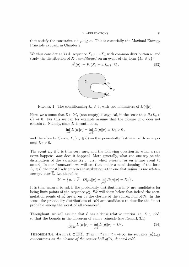
Figure 1. The conditionning Ln ∈ E, with two minimizers of D(·‖ν).
Here, we assume that E ⊂ M1 (non-empty) is atypical, in the sense that Pν(Ln ∈E) → 0. For this we can for example assume that the closure of E does notcontain ν. Namely, since D is continuous,
infµ∈E
D(µ‖ν) = infµ∈E
D(µ‖ν) ≡ DE > 0 ,
and therefore by Sanov, Pν(Ln ∈ E) → 0 exponentially fast in n, with an expo-nent DE > 0.
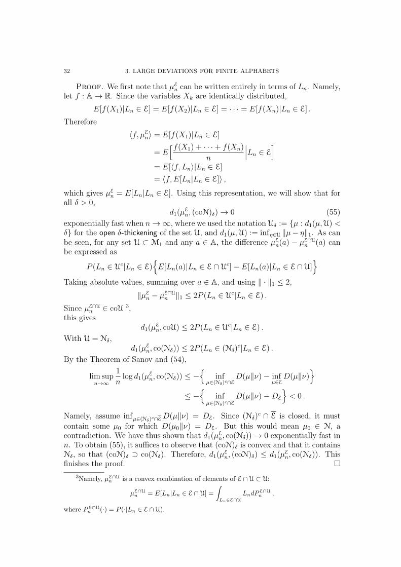
The event Ln ∈ E is thus very rare, and the following question is: when a rareevent happens, how does it happen? More generally, what can one say on thedistribution of the variables X1, . . . , Xn when conditioned on a rare event tooccur? In our framework, we will see that under a conditionning of the formLn ∈ E, the most likely empirical distribution is the one that infimizes the relativeentropy over E. Let therefore
N :=µ∗ ∈ E : D(µ∗‖ν) = inf
µ∈ED(µ‖ν) = DE
.
It is then natural to ask if the probability distributions in N are candidates forbeing limit points of the sequence µE
n. We will show below that indeed the accu-mulation points of µE
n are given by the closure of the convex hull of N. In thissense, the probability distributions of coN are candidates to describe the “mostprobable among the worst of all scenarios”.
Throughout, we will assume that E has a dense relative interior, i.e. E ⊂ intE,so that the bounds in the Theorem of Sanov coincide (see Remark 3.1):
infµ∈intE
D(µ‖ν) = infµ∈E
D(µ‖ν) = DE . (54)
Theorem 3.4. Assume E ⊂ intE. Then in the limit n→ ∞, the sequence (µEn)n≥1
concentrates on the closure of the convex hull of N, denoted coN.
32 3. LARGE DEVIATIONS FOR FINITE ALPHABETS
Proof. We first note that µEn can be written entirely in terms of Ln. Namely,
let f : A → R. Since the variables Xk are identically distributed,
E[f(X1)|Ln ∈ E] = E[f(X2)|Ln ∈ E] = · · · = E[f(Xn)|Ln ∈ E] .
Therefore
〈f, µEn〉 = E[f(X1)|Ln ∈ E]
= E[f(X1) + · · ·+ f(Xn)
n
∣∣∣Ln ∈ E
]
= E[〈f, Ln〉|Ln ∈ E]
= 〈f, E[Ln|Ln ∈ E]〉 ,which gives µE
n = E[Ln|Ln ∈ E]. Using this representation, we will show that forall δ > 0,
d1(µEn, (coN)δ) → 0 (55)
exponentially fast when n→ ∞, where we used the notation Uδ := µ : d1(µ,U) <δ for the open δ-thickening of the set U, and d1(µ,U) := infη∈U ‖µ− η‖1. As canbe seen, for any set U ⊂ M1 and any a ∈ A, the difference µE
n(a) − µE∩Un (a) can
be expressed as
P (Ln ∈ Uc|Ln ∈ E)
E[Ln(a)|Ln ∈ E ∩ Uc]− E[Ln(a)|Ln ∈ E ∩ U]
Taking absolute values, summing over a ∈ A, and using ‖ · ‖1 ≤ 2,
‖µEn − µE∩U
n ‖1 ≤ 2P (Ln ∈ Uc|Ln ∈ E) .
Since µE∩Un ∈ coU 3,
this givesd1(µ
En, coU) ≤ 2P (Ln ∈ Uc|Ln ∈ E) .
With U = Nδ,d1(µ
En, co(Nδ)) ≤ 2P (Ln ∈ (Nδ)
c|Ln ∈ E) .
By the Theorem of Sanov and (54),
lim supn→∞
1
nlog d1(µ
En, co(Nδ)) ≤ −
infµ∈(Nδ)c∩E
D(µ‖ν)− infµ∈E
D(µ‖ν)
≤ −
infµ∈(Nδ)c∩E
D(µ‖ν)−DE
< 0 .
Namely, assume infµ∈(Nδ)c∩ED(µ‖ν) = DE. Since (Nδ)
c ∩ E is closed, it must
contain some µ0 for which D(µ0‖ν) = DE. But this would mean µ0 ∈ N, acontradiction. We have thus shown that d1(µ
En, co(Nδ)) → 0 exponentially fast in
n. To obtain (55), it suffices to observe that (coN)δ is convex and that it containsNδ, so that (coN)δ ⊃ co(Nδ). Therefore, d1(µ
En, (coN)δ) ≤ d1(µ
En, co(Nδ)). This
finishes the proof.
3Namely, µE∩Un
is a convex combination of elements of E ∩ U ⊂ U:
µE∩U
n= E[Ln|Ln ∈ E ∩ U] =
∫
Ln∈E∩U
LndPE∩U
n,
where PE∩Un
(·) = P (·|Ln ∈ E ∩ U).
2. APPLICATIONS 33
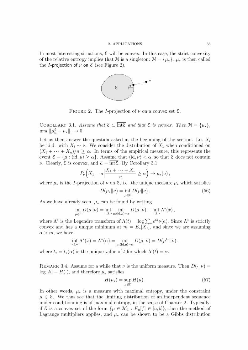
In most interesting situations, E will be convex. In this case, the strict convexityof the relative entropy implies that N is a singleton: N = µ∗. µ∗ is then calledthe I-projection of ν on E (see Figure 2).
ν
E µ∗
Figure 2. The I-projection of ν on a convex set E.
Corollary 3.1. Assume that E ⊂ intE and that E is convex. Then N = µ∗,and ‖µE
n − µ∗‖1 → 0.
Let us then answer the question asked at the beginning of the section. Let Xi
be i.i.d. with Xi ∼ ν. We consider the distribution of X1 when conditioned on(X1 + · · · + Xn)/n ≥ α. In terms of the empirical measure, this represents theevent E = µ : 〈id, µ〉 ≥ α. Assume that 〈id, ν〉 < α, so that E does not containν. Clearly, E is convex, and E = intE. By Corollary 3.1
Pν
(
X1 = a∣∣∣X1 + · · ·+Xn
n≥ α
)
→ µ∗(a) ,
where µ∗ is the I-projection of ν on E, i.e. the unique measure µ∗ which satisfies
D(µ∗‖ν) = infµ∈E
D(µ‖ν) . (56)
As we have already seen, µ∗ can be found by writing
infµ∈E
D(µ‖ν) = infx≥α
infµ:〈id,µ〉=x
D(µ‖ν) ≡ infx≥α
Λ∗(x) ,
where Λ∗ is the Legendre transform of Λ(t) = log∑
a etaν(a). Since Λ∗ is strictly
convex and has a unique minimum at m = Eν [X1], and since we are assumingα > m, we have
infx≥α
Λ∗(x) = Λ∗(α) = infµ:〈id,µ〉=α
D(µ‖ν) = D(µt∗‖ν) ,
where t∗ = t∗(α) is the unique value of t for which Λ′(t) = α.
Remark 3.4. Assume for a while that ν is the uniform measure. Then D(·‖ν) =log |A| −H(·), and therefore µ∗ satisfies
H(µ∗) = supµ∈E
H(µ) . (57)
In other words, µ∗ is a measure with maximal entropy, under the constraintµ ∈ E. We thus see that the limiting distribution of an independent sequenceunder conditionning is of maximal entropy, in the sense of Chapter 2. Typically,if E is a convex set of the form µ ∈ M1 : Eµ[f ] ∈ [a, b], then the method ofLagrange multipliers applies, and µ∗ can be shown to be a Gibbs distribution
34 3. LARGE DEVIATIONS FOR FINITE ALPHABETS
with potential f and a well defined inverse temperature β (depending on [a, b]).We will come back to this application in Chapter 4.
3. The Theorem of Sanov for Pairs
The empirical measure Ln studies the frequency with which the individual lettersappear in a sample of size n. More detailed information can be extracted fromthe sample by studying the occurence of words. The case of words of size twoalready contains the main difficulty, and we shall stick to this case.
The empirical pair measure is the probability distribution on words of size two,defined by
L2n :=
1
n
n∑
j=1
δ(Xj ,Xj+1) . (58)
As will be seen, it is convenient to define L2n by identifying thatXn+1 ≡ X1 (which,
when n is large, has no influence on the statistics of pairs). L2n ∈ M1(A
2), theset of probability distributions on pairs (a, b) ∈ A
2. A generic element of M1(A2)
will usually be denoted by π. The topology on M1(A2) is that of the L1-norm,
defined as before:
‖π − π′‖1 :=∑
a,b
|π(a, b)− π′(a, b)| .
The marginal of the first (resp. second) coordinate of π, denoted π ∈ M1(A)(resp. π ∈ M1(A)), is given by π(a) :=
∑
b π(a, b) (resp. π(b) :=∑
a π(a, b)). By
the cyclicity condition Xn+1 ≡ X1, we actually have L2n ∈ M
cycl1 (A2), where
Mcycl1 (A2) := π ∈ M1(A
2) : π = π .We of course expect L2
n to be close to ν ⊗ ν when n is large. Actually, as canbe shown using the Ergodic Theorem of Birkhoff (or simply the Strong Law ofLarge Numbers, if suitably applied), when n→ ∞,
L2n ⇒ ν ⊗ ν Pν − a.s. (59)
We will describe the concentration of L2n in the vincinity of ν ⊗ ν in terms of the
following rate function: if π ∈ Mcycl1 (A2),
I2ν (π) :=∑
a,b
π(a, b) logπ(a, b)
π(a)ν(b). (60)
Observe that if D denotes the relative entropy between distributions on M1(A2)
(see Definition 3.1), then
I2ν (π) = D(π‖π ⊗ ν) , (61)
and not D(π‖ν ⊗ ν) as one could have naively expected. The presence of π ⊗ νcomes from the fact that unlike single letters, words can overlap. Nevertheless,I2ν has the expected properties (compare with Proposition 3.1):
Proposition 3.4. I2ν : Mcycl1 (A2) → R has the following properties:
(1) I2ν (π) ≥ 0, with equality if and only if π = ν ⊗ ν.
3. THE THEOREM OF SANOV FOR PAIRS 35
(2) π → I2ν (π) is strictly convex, except on segments [π, π′] which satisfyπ(a, b)/π(a) = π′(a, b)/π′(a), on which it is affine.
Proof. (Similar to proof of Proposition 3.1.) Write
I2ν (π) =∑
a,b
π(a)ν(b)ψ(Xa,b) ,
where ψ(x) := x log x andXa,b :=π(a,b)
π(a)ν(b). By Jensen’s Inequality, I2ν (π) ≥ ψ(1) =
0, with equality if and only if π(a, b) = π(a)ν(b). But since π ∈ Mcycl1 (A2), this
implies π = π = ν, and so π = ν ⊗ ν. Convexity follows from the representation(61) and from (3) in Proposition 3.1, which implies that π 7→ D(π‖π ⊗ ν) isconvex.
Theorem 3.5 (Theorem of Sanov for pairs). Let X1, X2, . . . be i.i.d. with com-mon distribution ν. For all E ⊂ M1(A
2),
− infπ∈intE
I2ν (π) ≤ lim infn→∞
1
nlogPν(L
2n ∈ E) (62)
≤ lim supn→∞
1
nlogPν(L
2n ∈ E) ≤ − inf
π∈EI2ν (π) , (63)
Proof. Let as before L2n ⊂ M
cycl1 (A2) denote the set of (cyclic) types of
size n, i.e. the set of all empirical measures L2n associated to the sequences
(X1, . . . , Xn) ∈ An. We start as in the proof of Theorem 3.5, and decompose as
we did in (38):
Pν(L2n ∈ E) =
∑
π∈E∩L2n
Pν(L2n = π) . (64)
The key of the proof is to observe that a sequence X = (X1, . . . , Xn) can beencoded into a path in a graph with vertices A, and that L2
n can be read off thepath by counting the number of times each edge is visited.
A multigraph (with vertex set A), G = (A, E), is specified by a multiset E oforiented edges, that is, a set of pairs (a, b) with a, b ∈ A, in which the same paircan appear more than once. The multiset E is therefore completely characterizedby a family of numbers kG(a, b) ∈ 0, 1, . . . , n, where kG(a, b) gives the numberof times the edge (a, b) appears in E.
We associate to each sample X = (X1, . . . , Xn) a multigraph G(X) = (A, E(X))by walking along the vertices A and adding a new edge (a, b) to the edge-set eachtime it is traversed. In the end, the edge (a, b) appears the same number of timesin E(X) as the number of is for which (Xi, Xi+1) = (a, b). By the identificationXn+1 ≡ X1, the path is back at its starting pointX1 at time n+1. The multigraphG(X) contains all the information about L2
n: for all pair (a, b),
L2n(a, b) =
kG(X)(a, b)
n.
36 3. LARGE DEVIATIONS FOR FINITE ALPHABETS
For a given π ∈ L2n, of the form π = k
n, let Gπ denote the multigraph associated
to π, in which the edge (a, b) appears exactly k(a, b) ≡ nπ(a, b) times. Then
Pν(L2n = π) =
∑
X:G(X)=Gπ
Pν(X) .
Clearly, all the sequences X appearing in the sum have same probability. Namely,in each of them, the symbol a ∈ A appears exactly
∑
b kG(X)(a, b) =∑
b k(a, b) ≡k(a) times, and so
Pν(L2n = π) =
(∏
a
ν(a)k(a))
♯X : G(X) = Gπ . (65)
Let G′π denote the graph with vertex set A such that each pair of points (a, b)
is joined by exactly k(a, b) distinct oriented edges. Now, the number of elementsin X : G(X) = Gπ can be obtained by first counting the number of distinctEulerian paths on G′
π (that is paths that visit each edge of G′π exactly once), and
then take care of the number of overcountings that have been made. Since exactly∏
a,b k(a, b)! distinct Eulerian paths yield the same sequence X we get
♯X : G(X) = Gπ = cycl(π) · ♯Eulerian paths on G′π
∏
a,b k(a, b)!,
where 1 ≤ cycl(π) ≤ n is a number that accounts for the fact that each Eulerianpath can yields to at most n distinct sequencesX, obtained by cyclic permutation.
Lemma 3.5. For all π = kn∈ L2
n,∏
a
(k(a)− 1)! ≤ ♯Eulerian paths on G′π ≤ |A|
∏
a
k(a)! . (66)
Since 1 ≤ ∏
a k(a) ≤ n|A|, we can thus write (65) as:
Pν(L2n = π) =
(∏
a
ν(a)k(a))
eO(logn)
∏
a k(a)!∏
a,b k(a, b)!, (67)
uniformly in π ∈ L2n. Using the Stirling formula for each of the factorials k(a, b)!,
k(a)!, gathering carefully the terms and remembering (60),
Pν(L2n = π) = e−nI2ν (π)+O(logn) . (68)
The rest of the proof proceeds as in Theorem 3.5. For example, for the upperbound,
Pν(L2n ∈ E) ≤ |E ∩ L2
n| supπ∈E∩L2
n
Pν(L2n = π)
≤ |E ∩ L2n|eO(logn) exp
(− n inf
π∈E∩L2n
I2ν (π))
≤ |E ∩ L2n|eO(logn) exp
(− n inf
π∈EI2ν (π)
),
from which (63) follows, since |E ∩ L2n| ≤ |L2
n| ≤ (n+ 1)|A2|.
The Theorem of Sanov for pairs will be used later when studying large deviationsfor Markov chains. COMPLETER