Elements of Classical Field Theory

C6, Michaelmas 2017

Joseph Conlona

aRudolf Peierls Centre for Theoretical PhysicsUniversity of Oxford

OX1 3PN Oxford, United Kingdom

Please send corrections to joseph.conlon@physics.ox.ac.uk.

The parts of the script that are colored blue are not covered in the lecture. They will howeverbe discussed (at least in parts) in the exercises.

The parts of the script that are colored red are strictly non-examinable and will not be coveredin the exercises. They represent, for those who are interested, a more advanced gloss on thematerial.

These notes are adapted from the lectures notes of Uli Haisch.

1 Classical Field Theory

We start by discussing various aspects of classical fields. This will lay the groundwork for thesubsequent analysis of qauntum fields, as well as illustrating the dynamics of fields beyondwhat we will be able to analyse in the quantum theory.

1.1 Dynamics of Fields

A field is a quantity that can have a different value at every point of a space(-time) x = (t,x).The spatial coordinate x may parametrise space itself, but also may restrict to the interior(or surface) of a material - it depends on what the field is describing.

The particular difference of fields is that they involve an infinite number of degrees of free-dom. While classical particle mechanics deals with a finite number of generalized coordinatesqa(t), indexed by a label a, in field theory we are interested in the dynamics of fields

φa(t,x) , (1.1)

where both a and x are considered as labels. We are hence dealing with an infinite number ofdegrees of freedom (dofs), at least one for each point x in space. Notice that the concept ofposition has been relegated from a dynamical variable in particle mechanics to a mere labelin field theory.

1

What does every point in space(-time) mean physically? If we take a fielddefined on spacetime, then this implies that the value of the field at one point,and the value at another point separated by 10−25 metres, are physically separatedynamical quantities. There are, furthermore, an infinite number of dynamicalquantities going down to ever smaller and smaller scales. By writing a field φ(x, t),and describing its dynamics, we are also talking about the dynamics of this infinitenumber of quantities defined on truly microscopic scales.

Actually, we know this must ultimately be wrong physics. In condensed mattersystems, this notion is going to break down when we get to distances much smallerthan a lattice spacing - at sub-atomic separations, it really does not make senseto talk about the value of a field φ(x, t). Even in particle physics, where we mightthink that space makes sense down to arbitrarily small distances, any classicalpicture of space will still fail at small enough distances (once quantum gravitykicks in).

But yet we still talk about fields with infinite numbers of degrees of freedom, andin practice what happens at the very shortest of distances turns out to decouplewhen we get to longer distances. The field φ(x, t) does contain short-distancedynamics in it - but it also drops out from the long-distance questions we wantto pose. That this happens is true but deeply non-obvious, and arises from thephysics of renormalisation.

Lagrangian and Action

The dynamics of the fields is governed by the Lagrangian. In all the systems we will studyin this course, the Lagrangian is a function of the fields φa and their derivatives ∂µφa,

1 andgiven by

L(t) =

∫d3xL(φa, ∂µφa) , (1.2)

where the official name for L is Lagrangian density, but is in practice often simply calledthe Lagrangian. I am now also going to assume that the field is defined on four dimensions,three spatial and one time (this is an assumption - there are many interesting and physicallyimportant field theories that are defined on dimensions less than three).

For any time interval t ∈ [t1, t2], the action corresponding to (1.2) reads

S =

∫ t2

t1

dt

∫d3xL =

∫d4xL . (1.3)

Recall that in classical mechanics L depends only on qa and qa, but not on the second timederivatives of the generalized coordinates. In field theory we similarly restrict to LagrangiansL depending on φa and φa. Furthermore, with an eye on Lorentz invariance, we will onlyconsider Lagrangians depending on ∇φa and not higher derivatives.

Notice that employing c = ~ = 1, i.e., working with natural units, the dimension ofthe action is [S] = 0. With (1.3) and [d4x] = −4, it follows that the Lagrangian must

1If there is no (or only little) room for confusion, we will often drop the arguments of functions and writeφa = φa(x) etc. to keep the notation short.

2

necessarily have [L] = 4. Other objects that we will use frequently to construct Lagrangiansare derivatives, masses, couplings, and most importantly fields. The dimensions of the formertwo objects are [∂µ] = 1 and [m] = 1, while the dimensions of the latter two quantities dependon the specific type of coupling and field one considers. We therefore postpone the discussionof the mass dimension of couplings and fields to the point when we meet the relevant buildingblocks.

Principle of Least Action

As with particles, yhe dynamical behavior of fields can be determined by the principle ofleast action. This principle states that when a system evolves from one given configuration toanother between times t1 and t2 it does so along a “path” in configuration space for which theaction is an extremum (usually a minimum) and hence satisfies δS = 0. This condition leadsto equations of motion:

δS =

∫d4x

{∂L∂φa

δφa +∂L

∂(∂µφa)δ(∂µφa)

}

=

∫d4x

{[∂L∂φa− ∂µ

(∂L

∂(∂µφa)

)]δφa + ∂µ

(∂L

∂(∂µφa)δφa

)}= 0 .

(1.4)

The last term is a total derivative and vanishes for any δφa that decays at spatial infinity andobeys δφa(t1,x) = δφa(t2,x) = 0. For all such paths, we obtain the Euler-Lagrange equationsof motion (EOMs) for the fields φa, namely

∂µ

(∂L

∂(∂µφa)

)− ∂L∂φa

= 0 . (1.5)

When we come to quantise fields, ultimately the most powerful approach is the use of thepath integral formalism, from which the principle of least action arises as a classical limit.However, the easier (but less powerful) approach comes from using a Hamiltonian as taughtin ordinary quantum mechanics.

Hamiltonian Formalism

The Hamiltonian formalism of classical mechanics starts with the Hamiltonian,

H(qi,pi, t) =∑

i

piqi(qi, pi, t)− L (1.6)

where the conjugate momentum

pi =∂L

∂qi. (1.7)

Field theory is ‘just’ the mechanics of systems with N → ∞ degrees of freedom. Forthe Hamiltonian formalism of field theory, as the degrees of freedom are φa(x), the conjugatemomentum variable (momentum density) is πa(x),

πa =∂L∂φa

. (1.8)

3

In terms of πa, φa, and L the Hamiltonian density is given by

H = πaφa − L , (1.9)

where, as in classical mechanics, we must eliminate φa in favor of πa everywhere in H. TheHamiltonian then simply takes the form

H =

∫d3xH . (1.10)

Note the expression for H is precisely as in the case of classical mechanics and is to be regardedas a function of φa and πa (no explicit inclusion of φa).

1.2 Noether’s Theorem

A field theory is not required to possess any particular symmetries, and perfectly consistentfield theories can be constructed which possess no special symmetry properties.

But, interesting field theories that we care about generally do have extra symmetry prop-erties. Familiar examples are spatial translation, spatial rotation, time translation invarianceand Lorentz symmetry. Less familiar examples are internal gauge or global symmetries (whichmay relate different types of particle to each other), chiral symmetries (multiplying fermionsfields by complex phases), or supersymmetries (which relate bosons and fermions).

The role of symmetries in field theory is therefore possibly even more important than inparticle mechanics. As with particle mechanics, a crucial aspect of symmetries is that theylead to the generation of conserved quantities. We therefore start here by recasting Noether’stheorem within a field theoretic framework.

Currents and Charges

The statement of Noether’s theorem is that every continuous symmetry of the Lagrangiangives rise to a conserved current Jµ(x), so that the EOMs (1.5) imply

∂µJµ = 0 , (1.11)

or in components dJ0/dt+∇ ·J = 0.2 To every conserved current there exists also a conserved(global) charge Q, i.e., a physical quantity which stays the same value at all times, defined as

Q =

∫

R3

d3x J0 . (1.12)

The latter statement is readily shown by taking the time derivative of Q,

dQ

dt=

∫

R3

d3xdJ0

dt= −

∫

R3

d3x∇ · J , (1.13)

2In quantum theory there can be exceptions to this, called ‘anomalies’, where symmetries of the classicalLagrangian cease are not symmetries of the quantum theory.

4

which is zero, provided we assume that J falls off sufficiently rapidly as |x| → ∞. Notice,however, that the existence of the conserved current J is much stronger than the existence ofthe (global) charge Q, because it implies that charge is in fact conserved locally. To see this,we define the charge in a finite volume V by

QV =

∫

V

d3x J0 . (1.14)

Repeating the above analysis, we find

dQV

dt= −

∫

V

d3x∇ · J = −∮

S

dS · J , (1.15)

where S denotes the area bounding V , dS is a shorthand for n dS with n being the outwardpointing unit normal vector of the boundary S, and we have used Gauss’ theorem. In physicalterms the result means that any charge leaving V must be accounted for by a flow of thecurrent 3-vector J out of the volume. This kind of local conservation law of charge holds inany local field theory.

Proof of Theorem

In order to prove Noether’s theorem, we’ll consider infinitesimal transformations. This isalways possible in the case of a continuous symmetry. We say that δφa is a symmetry of thetheory if, under a field transformation

φa → φa + δφa, (1.16)

the Lagrangian changes by a total derivative

δL(φa) = ∂µJ µ(φa) , (1.17)

for a set of functions J µ. We then consider the transformation of L under an arbitrary changeof field δφa. Glancing at (1.4) tells us that in this case

δL =

[∂L∂φa− ∂µ

(∂L

∂(∂µφa)

)]δφa + ∂µ

(∂L

∂(∂µφa)δφa

). (1.18)

When the EOMs are satisfied than the term in square bracket vanishes so that we are simplyleft with the total derivative term. For a symmetry transformation satisfying (1.17), therelation (1.18) hence takes the form

∂µJ µ = δL = ∂µ

(∂L

∂(∂µφa)δφa

), (1.19)

or simply ∂µJµ = 0 with

Jµ =∂L

∂(∂µφa)δφa − J µ , (1.20)

5

which completes the proof. Notice that if the Lagrangian is invariant under the infinitesimaltransformation δφa, i.e., δL = 0, then J µ = 0 and Jµ contains only the first term on theright-hand side of (1.20).

We stress that that our proof only goes through for continuous transformations for whichthere exists a choice of the transformation parameters resulting in a unit transformation, i.e.,no transformation. An example is a Lorentz boost with some velocity v, where for v = 0 thecoordinates x remain unchanged. There are examples of discrete symmetry transformationswhere this does not occur. E.g., a parity transformation P does not have this property, andNoether’s theorem is not applicable then.

Energy-Momentum Tensor

Recall that in classic particle mechanics, spatial translation invariance gives rise to the con-servation of momentum, while invariance under time translations is responsible for the con-servation of energy. What happens in classical field theory? To figure it out, let’s have a lookat infinitesimal translations

xν → xν − εν =⇒ φa(x)→ φa(x+ ε) = φa(x) + εν∂νφa(x) , (1.21)

where the sign in the field transformation is plus, instead of minus, because we are doing anactive, as opposed to passive, transformation. If the Lagrangian does not explicitly dependon x but only through φa(x) (which will always be the case in the Lagrangians discussed inthe course), the Lagrangian transforms under the infinitesimal translation as

L → L+ εν∂νL . (1.22)

Since the change in L is a total derivative, we can invoke Noether’s theorem which givesus four conserved currents T µν = (Jµ)ν one for each of the translations εν (ν = 0, 1, 2, 3).From (1.20) and (1.21) we readily read off the explicit expressions for T µν ,

T µν =∂L

∂(∂µφa)∂νφa − δµνL . (1.23)

This quantity is called the energy-momentum (or stress-energy) tensor. It has dimension[T µν ] = 4 and satisfies

∂µTµν = 0 . (1.24)

The four “conserved charges” are (µ = 0, 1, 2, 3)

P µ =

∫d3xT 0µ , (1.25)

Specifically, the “time component” of P µ is

P 0 =

∫d3xT 00 =

∫d3x

(πaφa − L

), (1.26)

which (looking at (1.9) and (1.10)) is nothing but the Hamiltonian H. We thus conclude thatthe charge P 0 is the total energy of the field configuration, and it is conserved. In fields theory,

6

energy conservation is thus a pure consequence of time translation symmetry, like it was inparticle mechanics. Similarly, we can identify the charges P i (i = 1, 2, 3),

P i =

∫d3xT 0i = −

∫d3x πa∂iφa , (1.27)

as the momentum components of the field configuration in the three space directions, and theyare of course also conserved.

1.3 Symmetries and the Lorentz Group

In general, there are many different symmetry that can occur in physics. A symmetry trans-formation is, generally, an operation you can perform on a system that transforms it back toitself. In physics, symmetries normally refer to symmetries of the underlying equations. Muchinteresting physics - including both superconductivity and the properties of the Higgs boson- can be understood as examples of where there is a symmetry of the equations that is not asymmetry of the solution.

We are not going to give a formal mathematical presentation of group theory in theselectures (see the previous C6 lecture notes by John Chalker and Andre Lukas for an account).However, one concept of general importance is that of a representation of a symmetry. Rep-resentations refer to the distinct ways an abstract symmetry can be concretely realised, bymapping each symmetry transformation gi onto an n×n matrix Gi acting on an n-dimensionalvectors. Examples are the 3-dimensional vector representation of spatial rotations or the ten-dimensional symmetric tensor (metric) representation of Lorentz transformations in generalrelativity.

One extremely important example of a symmetry is that of the Lorentz group. The Lorentzgroup L is of fundamental importance for the construction of relativistic field theories, as Lis associated with the symmetry of 4-dimensional space-time. We therefore now consider theform of the Lorentz group in some more detail.

Using the Minkowski metric η = diag (1,−1,−1,−1), the Lorentz group L consists of thereal 4× 4 matrices Λ that satisfy

η = ΛT ηΛ , (1.28)

which written in components (µ, ν, ρ, σ = 0, 1, 2, 3) takes the form

ηµν = ησρΛµρΛν

σ . (1.29)

It is readily seen that the transformations

xµ → Λµνx

ν , (1.30)

with Λ satisfying (1.28) leave the distance ds2 invariant. Setting for simplicity the speed oflight c to 1, one has

ds2 = ηµνdxµdxν → ηµνΛµ

ρdxρΛν

σdxσ = ηρσdx

ρdxσ = ds2 . (1.31)

The Lorentz transformations (LTs) (1.30) therefore preserve distance as measured by theMinkowski metric.

7

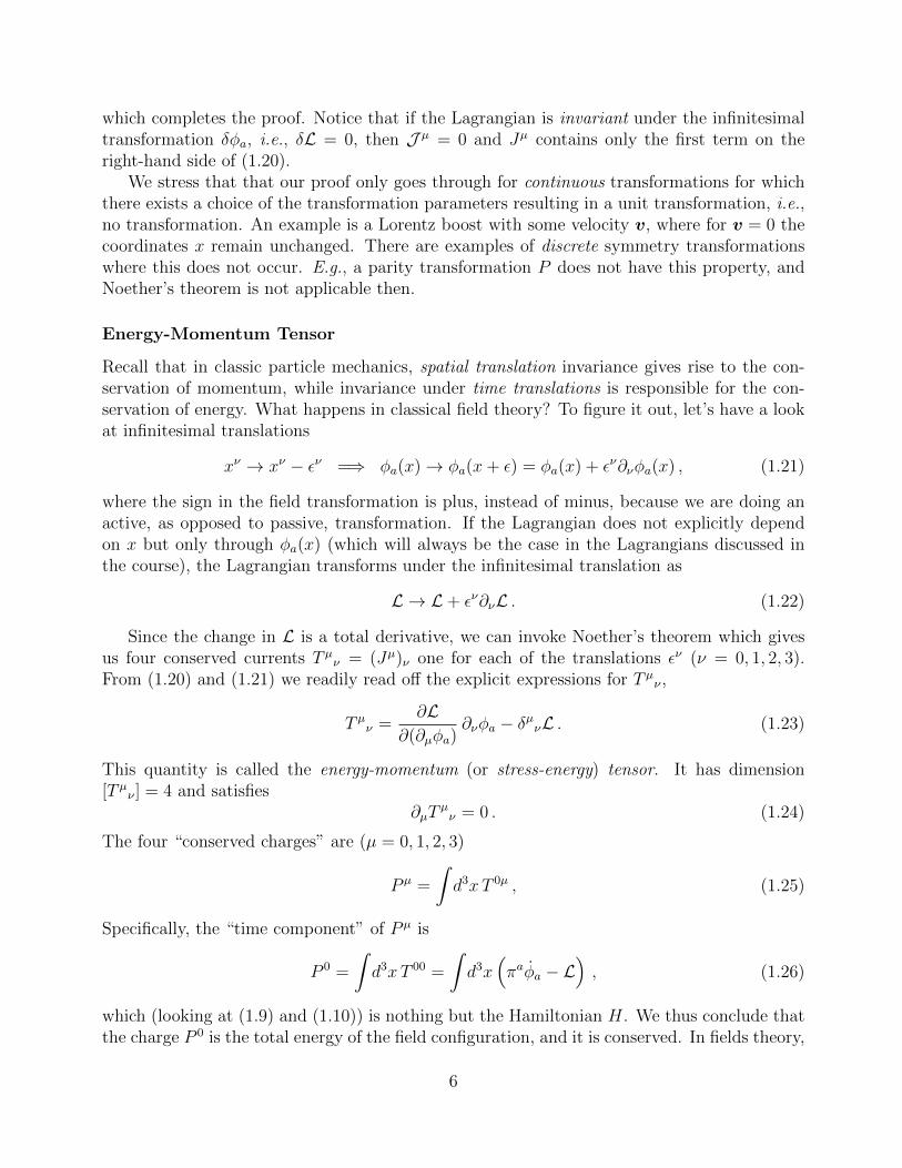
4.1. SYMMETRIES 43

det(!) !00 name contains given by

+1 ! 1 L!+ 14 L!

+

+1 " #1 L"+ PT PTL!

+

#1 ! 1 L!# P PL!

+

#1 " #1 L"# T TL!

+

Table 4.1: The four disconnected components of the Lorentz group. The union L+ = L!+ $ L"

+ is also called theproper Lorentz group andL! = L!

+$L!# is called the orthochronosLorentz group (as it consists of transformations

preserving the direction of time). L!+ is called the proper orthochronos Lorentz group.

O satisfying OT O = 1 and det(O) = 1. Writing O = 1 + iT with (purely imaginary) generators T , the relationOT O = 1 implies T = T † and, hence, that the Lie-algebra of SO(3) consists of 3 % 3 anti-symmetric matrices(multiplied by i). A basis for this Lie algebra is provided by the three matrices Ti defined by

(Ti)jk = #i!ijk , (4.16)

which satisfy the commutation relations[Ti, Tj] = i!ijkTk . (4.17)

These are the same commutation relations as in Eq. (4.13) and, hence, the Ti form a three-dimensional (irreducible)representation of (the Lie algebra of) SU(2). This representation must fit into the above classification of SU(2)representations by an integer or half-integer number j and, simply on dimensional grounds, it has to be identifiedwith the j = 1 representation.

4.1.4 The Lorentz groupThe Lorentz group is of fundamental importance for the construction of field theories. It is the symmetry associatedto four-dimensional Lorentz space-time and should be respected by field theories formulated in Lorentz space-time.Let us begin by formally defining the Lorentz group. With the Lorentz metric " = diag(1, #1, #1, #1) the Lorentzgroup L consists of real 4 % 4 matrices ! satisfying

!T "! = " . (4.18)

Special Lorentz transformations are the identity 14, parityP = diag(1, #1, #1, #1), time inversionT = diag(#1, 1, 1, 1)and the product PT = #14. We note that the four matrices {14, P, T, PT } form a finite sub-group of the Lorentzgroup. By taking the determinant of the defining relation (4.18) we immediately learn that det(!) = ±1 for allLorentz transformations. Further, if we write out Eq. (4.18) with indices

"µ!!µ"!

!# = ""# (4.19)

and focus on the component # = $ = 0 we conclude that (!00)

2 = 1 +!

i(!i0)

2 ! 1, so either !00 ! 1

or !00 " #1. This sign choice for !0

0 combined with the choice for det(!) leads to four classes of Lorentztransformations which are summarised in Table 4.1. Also note that the Lorentz group contains three-dimensionalrotations since matrices of the form

! =

"1 00 O

#(4.20)

satisfy the relation (4.18) and are hence special Lorentz transformations as long as O satisfies OT O = 13.To find the Lie algebra of the Lorentz group we write! = 14+iT + . . . with purely imaginary 4%4 generators

T . The defining relation (4.18) then implies for the generators that T = #"T T ", so T must be anti-symmetricin the space-space components and symmetric in the space-time components. The space of such matrices is six-dimensional and spanned by

Ji =

"0 00 Ti

#, K1 =

$%%&

0 i 0 0i 0 0 00 0 0 00 0 0 0

'(() , K2 =

$%%&

0 0 i 00 0 0 0i 0 0 00 0 0 0

'(() , K3 =

$%%&

0 0 0 i0 0 0 00 0 0 0i 0 0 0

'(() , (4.21)

Figure 1.1: The four disconnected components of the Lorentz group - these consist of’ordinary’ Lorentz transformations that may also be multiplied by Parity and Time-reversal.

Let us examine the consequences of (1.28). First, we take its determinant

det (η) = det(ΛT)

det (η) det (Λ) , (1.32)

from which we deduce thatdet (Λ) = ±1 . (1.33)

The case of det (Λ) = +1 (−1) corresponds to proper (improper) LTs and the associated sub-group is denoted L+ (L−). This implies that parity or space-inversion P = diag (1,−1,−1,−1)as well as time-reversal T = diag (−1, 1, 1, 1) are improper LTs and as such part of L−. Second,we look at the component η00, in which case one finds from (1.29) the relation

1 = ησρΛ0ρΛ0

σ =(Λ0

0

)2 −∑

i=1,2,3

(Λi

0

)2. (1.34)

It follows that|Λ0

0| ≥ 1 . (1.35)

When Λ00 ≥ 1 the LT is said to be orthochronous and part of L↑, while Λ0

0 ≤ −1 gives anon-orthochronous LT which belongs to L↓. In consequence, the Lorentz group consists outof four classes of LTs as illustrated in Figure 1.1

Let us have a look at some simple example of LTs: an ordinary spatial rotation by theangle θ about the z-axis, and then a boost by v < 1 along the x-axis

Λµν =

1 0 0 0

0 cos θ − sin θ 0

0 sin θ cos θ 0

0 0 0 1

, Λµ

ν =

γ −γv 0 0

−γv γ 0 0

0 0 1 0

0 0 0 1

, (1.36)

with γ = (1− v2)−1/2. In fact, any 3-dimensional rotation

Λµν =

(1 0

0 O

), (1.37)

8

44 CHAPTER 4. CLASSICAL FIELD THEORY

(j+, j!) dimension name symbol(0, 0) 1 scalar !(1/2, 0) 2 left-handed Weyl spinor "L

(0, 1/2) 2 right-handedWeyl spinor "R

(1/2, 0) ! (0, 1/2) 4 Dirac spinor #(1/2, 1/2) 4 vector Aµ

Table 4.2: Low-dimensional representations of the Lorentz group.

where Ti are the generators (4.16) of the rotation group. Given the embedding (4.20) of the rotation group intothe Lorentz group the appearance of the Ti should not come as a surprise. It is straightforward to work out thecommutation relations

[Ji, Jj ] = i$ijkJk , [Ki, Kj ] = "i$ijkJk , [Ji, Kj] = i$ijkKk . (4.22)

The above matrices can also be written in a four-dimensional covariant form by introducing six 4#4matrices %µ! ,labelled by two anti-symmetric four-indices and defined by

(%µ!)"# = i(&"

µ&!# " &µ#&"!) . (4.23)

By explicit computation one finds that Ji = 12$ijk%jk andKi = %0i. Introducing six independent parameters $µ! ,

labelled by an anti-symmetric pair of indices, a Lorentz transformation close to the identity can be written as

!"# $ '"

# " i

2$µ!(%µ!)"

# = '"# + $"

#; . (4.24)

The commutation relations (4.22) for the Lorentz group are very close to the ones for SU(2) in Eq. (4.13). Thisanalogy can be made even more explicit by introducing a new basis of generators

J±i =

1

2(Ji ± iKi) . (4.25)

In terms of these generators, the algebra (4.22) takes the form

[J±i , J±

j ] = i$ijkJ±k , [J+

i , J!j ] = 0 , (4.26)

that is, precisely the form of two copies (a direct sum) of two SU(2) Lie-algebras. Irreducible representations of theLorentz group can therefore be labelled by a pair (j+, j!) of two spins and the dimension of these representationsis (2j++1)(2j!+1). A list of a few low-dimensional Lorentz-group representations is provided in Table 4.2. Fieldtheories in Minkowski space usually require Lorentz invariance and, hence, the Lorentz group is of fundamentalimportance for such theories. Since it is related to the symmetries of space-time it is often also referred as externalsymmetry of the theory. The classification of Lorentz group representations in Table 4.2 provides us with objectswhich transform in a definite way under Lorentz transformations and, hence, are the main building blocks ofsuch field theories. In these lectures, we will not consider spinors in any more detail but focus on scalar fields!, transforming as singlets, ! % ! under the Lorentz group, and vector fields Aµ, transforming as vectors,Aµ % !µ

!A! .

4.2 General classical field theory4.2.1 Lagrangians and Hamiltonians in classical field theoryIn this subsection, we develop the general Lagrangian and Hamiltonian formalism for classical field theories.This formalism is in many ways analogous to the Lagrangian and Hamiltonian formulation of classical mechan-ics. In classical mechanics the main objects are the generalised coordinates qi = qi(t) which depend on timeonly. Here, we will instead be dealing with fields, that is functions of four-dimensional coordinates x = (xµ)on Minkowski space. Lorentz indices µ, (, · · · = 0, 1, 2, 3 are lowered and raised with the Minkowski metric(&µ!) = diag(1, "1, "1, "1) and its inverse &µ! . For now we will work with a generic set of fields !a = !a(x)before discussing scalar and vector fields in more detailed in subsequent sections. Recall that the Lagrangian in

Figure 1.2: Low-dimensional representations of the Lorentz group.

leaves ds2 invariant, since one has OTO = OOT = 13 by definition, if O is an element of the3-dimensional rotation group SO(3).3

Any Lorentz transformation can be decomposed as the product of a rotation, a boost,space-inversion P , and time-reversal T . Let us concentrate on the continuous transformations.Since there are three rotations and three boosts, one for each space direction, the continuousLTs are described in terms of six parameters. To find the corresponding six generators, i.e., abasis of transformation matrices that describes infinitesimal rotations and boosts, we write

Λ = 14 + iM , (1.38)

where M are purely imaginary 4 × 4 matrices. Inserting this linearized LT into the definingrelation (1.28), implies

M = −ηMT η . (1.39)

This tells us that the generators M must be anti-symmetric in the space-space components,but symmetric in the space-time components. The space of such matrices has indeed dimensionsix and is spanned by the set (i = 1, 2, 3)

Ji =

(0 0

0 Mi

),

K1 =

0 i 0 0

i 0 0 0

0 0 0 0

0 0 0 0

, K2 =

0 0 i 0

0 0 0 0

i 0 0 0

0 0 0 0

, K3 =

0 0 0 i

0 0 0 0

0 0 0 0

i 0 0 0

.

(1.40)

Here (Mi)jk = −iεijk with εijk the fully anti-symmetric Levi-Civita tensor (ε123 = +1) are thegenerators of SO(3). It follows that the matrices Ji (Ki) generate rotations (boosts).

It is a matter of simple algebra to work out the commutation relations of the generatorsJi and Ki of the Lorentz group. One obtains

[Ji, Jj] = iεijkJk , [Ki, Kj] = −iεijkJk , [Ji, Kj] = iεijkKk , (1.41)

3The group of 3-dimensional orthogonal matrices is denoted by O(3), while its subgroup of matrices withdeterminant +1 is called the special orthogonal group SO(3). The difference between the two is the paritytransformation x→ −x, which is in O(3) but not in SO(3).

9

where [a, b] = ab − ba is the usual commutator. These relations look very similar to thecommutation relations of angular momentum or spin that you should know from quantummechanics (QM). To make the analogy between the Lorentz group and the Lie group SU(2)even more explicit, we introduce the following new basis of generators

J±i =1

2(Ji ± iKi) . (1.42)

In terms of these generators, it is straightforward to verify that the Lorentz Lie algebra (1.41)takes the form

[J±i , J±j ] = iεijkJ

±k , [J±i , J

∓j ] = 0 . (1.43)

This means that J+i and J−i independently obey the Lie algebra of SU(2). By analogy to the

spin quantum number, we can therefore introduce a pair (j+, j−) of two spins that characterizethe possible representations of the Lorentz group. The states within a representation arefurther distinguished by the eigenvalues of J+

3 and J−3 , which can take the values m+ =−j+,−j+ + 1, . . . , j+ − 1, j+ and m− = −j−,−j− + 1, . . . , j− − 1, j−. The dimension, i.e., thenumber of distinct states in a given representation (j+, j−) is hence (2j+ + 1) (2j− + 1).

A list of some basic low-dimensional Lorentz-group representations is provided in Fig-ure 1.2. Field theories in Minkowski space usually require Lorentz invariance and, hence,the Lorentz group is of fundamental importance for such theories. Since it is related to thesymmetries of space-time it is often also referred as external symmetry of the theory. Theclassification of Lorentz group representations provides us with objects which transform ina definite way under LTs and thus these objects are the main building blocks of such fieldtheories. In what follows we will not deal with the spinor fields χL,R and ψ that describefermions (quarks and leptons). Our focus will be on scalar φ and vector Aµ fields, which havevery simple transformation properties under the Lorentz group:

φ→ φ , Aµ → ΛµνAν . (1.44)

1.4 Scalar Field Theories

We now apply the formalism described above to scalar field theories. These are the simplestclass of Lorentz invariant field theories, as they only involve fields transforming trivially underthe Lorentz group.

A Single Real Scalar Field

The Lagrangian density of a real scalar field φ is given by

L =1

2(∂µφ)2 − V (φ) , (1.45)

where the first term is referred to as kinetic energy (or kinetic term), while the second is knownas the scalar potential.4 Notice that φ corresponds to the (j+, j−) = (0, 0) representation ofthe Lorentz group. The dimension of the real scalar field is obviously [φ] = 1.

4Note that if this is expanded, it looks like φ2−(∇φ)2−V (φ). As ∇φ depends on the values of the individualfield degrees of freedom, it can also be viewed as a ‘potential’ term, with the Lagrangian then reflecting theparticle mechanics form of L = T − U .

10

The scalar potential can be written as

V =1

2m2φ2 +

∞∑

n=3

λnn!φn . (1.46)

Here m is the mass of φ (this will become clear later on) and the coefficients λn are calledcoupling constants. Dimensional analysis tells us that

[m] = 1 , [λn] = 4− n . (1.47)

The coupling terms in (1.46) fall into three different categories. First, dimension-threeterms with [λ3] = 1. For such terms, we can define a dimensionless parameter λ3/E, whereE has dimension of mass and represents the energy scale of the process of interest. Thismeans that ∆L3 = λ3 φ

3/(3!) is a small perturbation for high energies, i.e., E � λ3, but abig one at low energies, i.e., E � λ3. Such terms are called relevant, because they becomeand are most relevant at low energies which, after all, is where most of the physics that weexperience lies. In a relativistic quantum field theory (QFT), we have E > m, which meansthat we can always make this sort of perturbations small by taking λ3 � m. Second, termsof dimension four with [λ4] = 0. E.g., ∆L4 = λ4 φ

4/(4!). Such terms are small if λ4 � 1 andare called marginal. Third, operators with dimension of higher than four, having [λn] < 0. Inthis case the appropriate dimensionless parameters is (λnE

n−4) and terms ∆Ln = λn φn/(n!)

with n ≥ 5 are small (large) at low (high) energies. Such contributions are called irrelevant,since in daily life, meaning En−4 � λn, these terms do not matter.

As we will see later, it is typically impossible to avoid high-energy processes in QFT. Wehence might expect problems with irrelevant terms (or operators) that become important athigh energies. Indeed, these operators lead to non-renormalizable QFTs in which one cannotmake sense of the infinities at arbitrarily high energies. This does not mean that these theoriesare useless, it just means that they become incomplete at some energy scale and need to beembedded into an appropriate complete theory aka an ultraviolet (UV) completion. Let mealso add that the above naive assignment of relevant, marginal, and irrelevant operators is notalways carved in stone, since quantum corrections can sometimes change the character of anoperator.

Low-Energy Description

In typical applications of QFT only the relevant and marginal couplings are important. Thisis due to the fact that the irrelevant couplings become small at low energies, as we have seenabove. In practice this saves us, since instead of considering the infinite number of couplingterms in (1.46), only a handful are actually needed. E.g., in the case of the real scalar field φdescribed earlier, we only have to take into account two operators, namely ∆L3 = λ3 φ

3/(3!)and ∆L4 = λ4 φ

4/(4!), in the low-energy limit.Let us have a closer look at this issue. Suppose that at some day we discover the true

superduper theory aka the TOE that describes the world at very high energy scales. Whateverthis scale is, let’s call it Λ. Since it is an energy scale, we obviously have [Λ] = 1. What wewant to understand are the laws of physics at energy scales E that we can probe directly

11

in a laboratory, which given today’s standards, means E � Λ. Let us further suppose thatat energies of order E, the laws of physics are described by a real scalar field.5 This scalarfield will have some complicated coupling terms (1.46), where the precise form is dictated byall the stuff that is going on in the TOE. Can we get an idea about the interactions? Well,we can write our dimensionful coupling constants λn in terms of dimensionless couplings gn,multiplied by a suitable power of the relevant scale Λ,

λn =gn

Λn−4 . (1.48)

The exact values of the dimensionless couplings gn depend on the details of the TOE,6 so wehave to do some guesswork. Since the couplings gn are dimensionless, 1 looks like a pretty goodand somehow a natural guess. Since we are not completely sure, let’s say gn = O(1). Thismeans that in a laboratory with E � Λ the coupling terms ∆Ln = λnφ

n/(n!) of (1.46) will besuppressed by powers of (E/Λ)n−4 if n ≥ 5. Given the CERN Large Hadron Collider (LHC)energy of around 1 TeV, this is a suppression by many orders of magnitude. E.g., for Λ =MP = 1016 TeV corresponding to the Planck mass MP , one has E/Λ = 10−16. It is this simpleargument based on dimensional analysis that ensures that we need to focus only on the firstfew terms in the interactions, namely those that are relevant and marginal. It also means thatif we only have access to low-energy experiments, it is going to be very difficult to figure outthe precise nature of the TOE, because its effects are highly diluted except for the relevantand marginal interactions. Some people therefore call the superduper theory that everybodyis looking for, not TOE, but TOENAIL, which stands for “theory of everything not accessiblein laboratories”.

Klein-Gordon Equation

Applying the Euler-Lagrange equations to (1.45) leads to

∂µ∂µφ+∂V

∂φ= 0 . (1.49)

This equation describes the dynamical evolution of the scalar field φ. The Laplacian inMinkowski space is sometimes denoted by � and ∂V/∂φ is commonly written as V ′. Inthis notation, the above equation reads �φ+ V ′ = 0.

For non-vanishing (interaction) coefficients λ3, λ4, . . . the equation is non-linear and solu-tions to (1.49) are difficult to find. We therefore simply ignore them for the time being andconsider only the free case. The dynamics of such a non-interacting massive real scalar fieldis encoded in the famous Klein-Gordon equation:

(� +m2

)φ = 0 , (1.50)

arising from the Lagrangian

L =1

2(∂µφ)2 − 1

2m2φ2 . (1.51)

5Of course, we know that this assumption is plain wrong, since the standard model (SM) of particle physicsis a non-abelian gauge theory with chiral fermions, but the same argument applies in that case.

6If we would know the precise structure of the TOE we could, in fact, calculate the couplings gn.

12

To find the solutions to the classical Klein-Gordon equation (1.51), we perform a Fouriertransform on the field φ,

φ(t,x) =

∫d3p

(2π)3eip·x φ(t,p) . (1.52)

In momentum space (1.51) simply reads

[∂2

∂t2+(p2 +m2

)]φ(t,p) = 0 , (1.53)

which tells us that for each value of p, the Fourier mode φ(t,p) obeys the equation of a simpleharmonic oscillator with frequency

ωp =√|p|2 +m2 . (1.54)

It is then not difficult to see that the most general solution of the classical Klein-Gordonequation is a linear superposition of simple harmonic oscillators,7

φ(x) =

∫d3p

(2π)31

2ωp

(a(p)e−ipx + a∗(p)eipx

), (1.55)

each vibrating at a different frequency with a different amplitude (the appearance of the specificcombination of coefficients a(p) and a∗(p) is dictated by the reality of the Klein-Gordon fieldφ). The 4-vector p in the exponents is understood as pµ = (ωp,p).

The decomposition (1.55) sees each individual Fourier mode evolving as a harmonic os-cilator. The main puzzling aspect is to understand why the amplitudes for the Fourier modeshave been written as a(p)

2ωprather than just a(p).

The reason why this is convenient is to notice that the measure d3p/(2π)3 1/(2ωp) is aLorentz-invariant quantity. This follows from “reverse engineering”

∫d3p

(2π)31

2ωp=

∫d3p

(2π)31

2p0

∣∣∣∣p0=ωp

=

∫d4p

(2π)3δ(p20−p2−m2)

∣∣p0>0

=

∫d4p

(2π)3δ(p2−m2)|p0>0 .

(1.56)From the latter result we can also figure out that the Lorentz-invariant delta function for3-momenta is

2ωp δ(3)(p− q) , (1.57)

since ∫d3p

2ωp2ωp δ

(3)(p− q) = 1 . (1.58)

The Lorentz invariance of the measure d3p/(2π)3 1/(2ωp) and its consequences, should be keptin mind, because these features will be important at several occasions later on.

The important physical implication is that quantizing the field φ is then the same asquantizing a infinite number of harmonic oscillators. A free field φ corresponds to an infinite

7The actual derivation of this result can be found on page 47 of the script by John Chalker and Andre Lukas.It is not repeated here.

13

number of non-interacting harmonic oscillators, and an interacting field φ corresponds to aninfinite number of interacting harmonic oscillator. You should already know how this is done inQM and we will see later on how it is done in QFT. As Sidney Coleman once said: “The careerof a young theoretical physicist consists of treating the harmonic oscillator in ever-increasinglevels of abstraction.”.

Lorentz Invariance

We want to confirm that a Lorentz Transformation

φ(x)→ φ′(x) = φ(Λ−1x) , (1.59)

leaves the the KG action invariant. Notice that the inverse Λ−1 appears here because we aredealing with an active transformation, in which the field is truly shifted.8 To see why thismeans that the inverse appears, it will suffice to consider a non-relativistic example such asa temperature field. Suppose we start with an initial field φ(x) which has a hotspot at, say,x = (1, 0, 0). Let’s now make a rotation x → Ox about the z-axis so that the hotspot endsup at x = (0, 1, 0). If we want to express the new field φ′(x) in terms of the old field φ(x),we have to place ourselves at x = (0, 1, 0) and ask what the old field looked like at the pointO−1x = (1, 0, 0) we came from. This O−1 is the origin of the Λ−1 factor in the argument ofthe transformed field in (1.59).

According to the LT (1.59), the transformation of the mass term is 1/2m2φ2(x) →1/2m2φ2(x′) with x′ = Λ−1x. The transformation of ∂µφ is

∂µφ(x)→transformation ∂µ(φ(x′)) = (Λ−1)νµ(∂νφ)(x′) . (1.60)

Here we have used that

∂µ =∂

∂xµ=

∂

∂(x′)ν∂(x′)ν

∂xµ= (Λ−1)νµ ∂

′ν . (1.61)

and wrote ∂′νφ(x′) = (∂νφ)(x′). Below we will also use the notation ∂µφ(x′) to denote thederivative with respect to x′ at x′. Using the defining property (Λ−1)ρµ(Λ−1)σν η

µν = ηρσ ofthe LTs, we thus find that the derivative term in the Klein-Gordon Lagrangian then transformsas

1

2(∂µφ(x))2 → 1

2(Λ−1)ρµ(∂ρφ)(x′)(Λ−1)σν(∂σφ)(x′) ηµν

=1

2(∂ρφ)(x′)(∂σφ)(x′) ηρσ

=1

2(∂µφ(x′))

2.

(1.62)

Putting things together, we see that the action of the Klein-Gordon theory is indeed Lorentzinvariant,

S =

∫d4xL(x)→

∫d4xL(x′) =

∫d4x′ L(x′) = S . (1.63)

8In passive transformations, it is the coordinates that are changed rather than the field.

14

Notice that changing the integration variables from d4x to d4x′, in principle introduces anJacobian factor det (Λ). This factor is, however, equal to 1 for LT connected to the identity,that we are dealing with (remember that 14 is part of the proper, orthochronous or restrictedLorentz group L↑+).

A similar calculation also shows that, as promised, the EOM of the Klein-Gordon field φ,as given in (1.50), are invariant,

(∂2 +m2

)φ(x)→

(∂2 +m2

)φ′(x)

=[(Λ−1)νµ∂ν(Λ

−1)ρµ∂ρ +m2]φ(x′)

=(ηνρ∂′ν∂

′ρ +m2

)φ(x′) = 0 .

(1.64)

Here we have used another common notation for the Laplacian, ∂µ∂µ = ∂2.Notice that the above explicit example shows that the Lagrangian formulation of field

theory makes it especially easy to discuss Lorentz invariance, since an EOM is automaticallyLorentz invariant if it follows from a Lagrangian that is a Lorentz scalar. This is an immediateconsequence of the principle of least action. If a LT leaves the Lagrangian unchanged, thenan extremum of the action will be transformed to another extremum of the action.

Conservation Laws

Let us derive the Hamiltonian density and the energy-momentum tensor for (1.45). Theconjugate momentum of φ is simply π = φ, and therefore

H =1

2π2 +

1

2(∇φ)2 + V . (1.65)

For the stress tensor we find from (1.23) the expression

T µν = (∂µφ)(∂νφ)− 1

2ηµν (∂ρφ)2 + ηµν V . (1.66)

Notice that the energy-momentum tensor of (1.45) immediately comes out symmetric, i.e.,Tµν = Tνµ. This is not always the case. In accordance with our general formula (1.26), wehence have

P 0 =

∫d3xT 00 =

∫d3x

(1

2π2 +

1

2(∇φ)2 + V

)=

∫d3xH = H . (1.67)

The energy is hence conserved in our real scalar theory. Analog relations hold for the spacecomponents P i, signalling 3-momentum conservation.

In classical particle mechanics, rotational invariance gives rise to conservation of angularmomentum. What is the analogy in field theory? What happens to the remaining three LTs,namely the boosts. What conserved quantity do they correspond to? In order to address thesequestions using Noether’s theorem, we first need the infinitesimal form of the LTs

Λµν = δµν + ωµν , (1.68)

15

where ωµν is infinitesimal. The condition (1.29) for Λ to be a LT becomes in infinitesimalform

ηµν = ηρσ (δµρ + ωµρ) (δνσ + ωνσ) = ηµν + ωµν + ωνµ +O(ω2) . (1.69)

This shows that ωµν must be an anti-symmetric matrix (a feature that I have stated beforewithout proof),

ωµν = −ωνµ . (1.70)

Notice that an anti-symmetric 4×4 matrix has six independent parameters, which agrees withthe number of different Lorentz transformations, i.e., three rotations and three boosts.

Applying the infinitesimal LT to our real scalar field φ, we have

φ(xλ)→ φ(xλ − ωλνxν) = φ(x)− ωλνxν∂λφ(x) , (1.71)

where the minus sign arises from the factor Λ−1 in (1.59). The variation of the field φ underan infinitesimal LT is hence given by

δφ = −ωµνxν∂µφ . (1.72)

By the same line of reasoning, one shows that the variation of the Lagrangian (as it is also aLorentz scalar) is

δL = −ωµνxν∂µL = −∂µ (ωµνxνL) , (1.73)

where in the last step we used the fact that ωµµ = 0 due to its anti-symmetry. The Lagrangianchanges by a total derivative, so we can apply Noether’s theorem (1.20) with J µ = −ωµνxνLto find the conserved current,

Jµ = − ∂L∂(∂µφ)

ωρνxν∂ρφ+ ωµνx

νL

= −ωρν[

∂L∂(∂µφ)

∂ρφ− δµρL]xν = −ωρνT µρxν .

(1.74)

Stripping off ωρν , we obtain six different currents, which we write as

(Iλ)µν = xµT λν − xνT λµ . (1.75)

These currents satisfy∂λ(Iλ)µν = 0 , (1.76)

and give (as usual) rise to six conserved charges . For µ, ν 6= 0, the LT is a rotation andthe three conserved charges give the total angular momentum of the field configuration (i, j =1, 2, 3):

Qij =

∫d3x

(xiT 0j − xjT 0i

). (1.77)

What’s about the boosts? In this case, the conserved charges are

Q0i =

∫d3x

(x0T 0i − xiT 00

). (1.78)

16

The fact that these are conserved tells us that

0 =dQ0i

dt=

∫d3xT 0i + t

∫d3x

dT 0i

dt− d

dt

∫d3x xiT 00

= P i + tdP i

dt− d

dt

∫d3x xiT 00 .

(1.79)

Yet, also the momentum P i is conserved, i.e., dP i/dt = 0, and we conclude that

d

dt

∫d3x xiT 00 =

d

dt

∫d3x xiH = const. (1.80)

This is the statement that the center of energy of the field travels with a constant velocity. Ina sense it’s a field theoretical version of Newton’s first law but, rather surprisingly, appearinghere as a conservation law. Notice that after restoring the label a our results for (Iλ)µν etc.also apply in the case of multicomponent fields.

Poincare Invariance

We now require that a physical system possesses both space-time translation (1.21) and Lorentzsymmetry. The symmetry group that includes both transformations is called the Poincaregroup. Notice that for any Poincare-invariant theory the two charge conservation equations(1.24) and (1.76) should hold.

This is only possible if the energy-momentum tensor T µν is symmetric. Applying first(1.76) and then (1.24), we have

0 = ∂λ(Iλ)µν = ∂λ(xµT λν − xνT λµ

)

= xµ∂λTλν + T λν∂λx

µ − xν∂λT λµ − T λµ∂λxν

= T λνδλµ − T λµδλν = T µν − T νµ .

(1.81)

This general result tells us that the expression of the energy-momentum tensor in any Poincare-invariant theory can be made symmetric without changing physics. The key to actually do it,lies in making use of the conservation law (1.24) in an appropriate way.

Discrete Internal Symmetries

So far we have only imposed external symmetries, such as Lorentz or Poincare symmetry,on our scalar theory. Let us also have a brief look at internal symmetries. An interesting(discrete) internal symmetry to be considered is a Z2 symmetry which acts as

φ(x)→ −φ(x) . (1.82)

This transformation leaves (1.45) invariant if the scalar potential V contains only terms withan even number of φ fields (but as it is not a continuous symmetry, we cannot use Noether’s

17

-v +vΦ

VHvL

VHΦL

Figure 1.3: Shape of the scalar potential for m2 ≥ 0 (solid line) and m2 < 0 (dashedline). In the latter case the positions of the minima are at φ = ±v = ±

√(−6m2)/λ.

The value of the potential at the minima is V (v) = V0 − (λv4)/24.

theorem to derive a conserved quantity). Restricting ourselves to relevant and marginal cou-plings, we write

V = V0 +1

2m2φ2 +

λ

4!φ4 . (1.83)

where we have added a constant term V0 to the potential. Note that the inclusion of theconstant term V0 leaves the EOM (1.49) unaltered.

Let us now study the simplest type of solutions to the real scalar theory with the poten-tial (1.83). A trivial solution of (1.49) is φ(x) = v = const., provided that

∂V

∂φ

∣∣∣∣φ=v

= 0 . (1.84)

This relation implies that we should look for the extrema of the potential (1.83). In fact,to minimize the energy (1.67) we should focus on the minima of V . Such solutions of theclassical theory are called vacua (or vacuum if there is a single one). Note that if the quarticcoupling λ is negative, the potential is not bounded from below and the energy of a constantfield configuration tends to minus infinity for large field values. To avoid such an unphysicalsituation, we simply assume λ > 0 in what follows.

The shape of the scalar potential V is shown in Figure 1.3. We see that one has todistinguish two cases. First, the case where m2 ≥ 0 (solid curve). In this situation there isa single minimum located at the origin φ = 0. This solution is mapped into itself under thetransformation (1.82) and we say that the symmetry is unbroken in this vacuum. The secondcase with m2 < 0 (dashed curve) is more interesting. In this case φ = 0 is a maximum, whilethere are two minima. These are located at

φ = ±v = ±√−6m2

λ. (1.85)

18

At the minima, the potential takes the value

V (v) = V0 +1

4m2v2 = V0 −

λv4

24. (1.86)

Notice that neither minimum is invariant under the Z2 symmetry. In fact, the minima areinterchanged under (1.82), and we say that the symmetry is spontaneously broken. In general,spontaneous symmetry breaking refers to the case where a symmetry of the underlying theoryis partially or fully broken by the vacuum solution of the theory. This concept of spontaneoussymmetry breaking is of fundamental importance in theoretical physics and we shall return toit later.

Continuous Internal Symmetries

Besides discrete symmetries, continuous internal symmetries also play an important role inparticle physics. We start our discussion by considering a scalar theory that involves two realscalar fields φ1,2 and combine these fields into a field vector

φ =

(φ1

φ2

). (1.87)

In the following we will be interested in theories that are invariant under SO(2) transformations(aka internal 2-dimensional rotations) that take the form

φ→ φ′ = Oφ . (1.88)

Since this transformation is the same at every space-time point, symmetries of this type arecalled global.9 The length of φ should be SO(2) invariant, which implies that

OTO = OOT = 12 , (1.89)

and we also require thatdet (O) = +1 . (1.90)

Proper 2-dimensional rotation matrices can be written as

O = eiαT , (1.91)

where α is a real parameter (the rotation angle) and T denotes the 2×2 matrix that generatesthe 2-dimensional rotations. A suitable choice of the generator reads

T =

(0 −ii 0

). (1.92)

Check that this indeed exponentiates to a standard rotation! Notice that SO(2) is said to bean abelian group, since

eiαT eiβT = eiβT eiαT = ei(α+β)T , (1.93)

9In a local transformation, the matrix O is allowed to differ between every point in space.

19

which means that the ordering of two successive group transformations (rotations) does notmatter.

For 3-dimensional rotations, things are a bit more complicated. Since there is now oneindependent rotation for each plane in three dimensions, the SO(3) group has 3 (3− 1) /2 =3 parameters αi (Euler angles) and three generators Ti (i = 1, 2, 3). Infinitesimal SO(3)transformations thus act on φ = (φ1, φ2, φ3)

T as φ → φ′ = φ + iαiTiφ. From (1.89) and(1.90) it follows that the generator Ti are hermitian and traceless:

(Ti)† = Ti , Tr (Ti) = 0 . (1.94)

A possible set of 3× 3 matrices with these properties is

T1 =

0 0 0

0 0 −i0 i 0

, T2 =

0 0 i

0 0 0

−i 0 0

, T3 =

0 −i 0

i 0 0

0 0 0

, (1.95)

which can be written in a more compact way as (Ti)jk = −iεijk (j, k = 1, 2, 3). By a straight-forward calculation, one can prove that the latter matrices satisfy the following Lie algebra

[Ti, Tj] = iεijkTk . (1.96)

These relations imply that two 3-dimensional rotations do not in general “commute”, whichis equivalent to the non-abelian character of SO(3).

Other examples of non-abelian groups are provided by the special unitary groups SU(n),which consist of all complex n× n matrices U satisfying

U †U = UU † = 1n , det (U) = +1 . (1.97)

The simplest non-trivial example of a special unitary group is SU(2). It has 22 − 1 = 3generators τi and close to the identity one can write the group transformations as U = 12+itiτi.From (1.97) it follows that the generators obey τ †i = τi and Tr (τi) = 0. A convenient choiceof the generators τi is

τi =σi2, (1.98)

where σi are the usual Pauli matrices given by

σ1 =

(0 1

1 0

), σ2 =

(0 −ii 0

), σ3 =

(1 0

0 −1

). (1.99)

Recalling that σiσj = δij12 + iεijkσk, it is easy to show that Tr (τiτj) = δij/2 and that theSU(2) generators fulfil the commutation relations

[τi, τj] = iεijkτk . (1.100)

Although they lead to the same commutation relations, SU(2) and SO(3) are not actuallythe same groups. They in fact differ in their global properties. SU(2) is a ‘double cover’ of

20

SO(3) - roughly, it contains two copies of SO(3). This is related to the fact that, under 2πrotations of SO(3) spinors return to minus themselves. This global minus sign means thatspinors should be viewed as representations of SU(2).

Interestingly, (1.96) and (1.100) are the same commutation relations. This means thatthe matrices τi and Ti form two different representations of the SU(2) Lie algebra. Therepresentation that is classified by the 2 × 2 matrices (1.98) is called fundamental. It actson a complex vector of size two and hence the dimension of the representation space is two.The representation where the generators are 3 × 3 matrices of the form (Ti)jk = −iεijk

(as

in (1.95))

is instead called the adjoint representation of SU(2). This representation acts on3-dimensional real vectors and therefore it has the dimension of SU(2) that is equal to three.

A Complex Scalar Field With a U(1) Symmetry

For the further discussion it will prove convenient to arrange the two real scalar fields thatwe have meet at the beginning of the previous subsection into a single complex Klein-Gordonfield defined as

ϕ =1√2

(φ1 + iφ2) . (1.101)

On this complex representation, the transformation (1.88) acts as follows(φ1

φ2

)→(

cosα − sinα

sinα cosα

)(φ1

φ2

)=⇒

(φ1

iφ2

)→(

cosα i sinα

i sinα cosα

)(φ1

iφ2

)

=⇒ φ1 + iφ2 → eiα (φ1 + iφ2) .

(1.102)

This means that all terms in the invariant Lagrangians we are looking for should be unchangedunder a rephasing of the φ field, aka a global U(1) transformation,

ϕ→ ϕ′ = eiαϕ , ϕ∗ → (ϕ′)∗ = e−iαϕ∗ . (1.103)

The different transformation properties of ϕ and ϕ∗ tell us that these fields carry charge 1 and−1, respectively.

Since ϕ and ϕ∗ carry a non-zero charge not all terms polynomial in the fields are allowedin the Lagrangian if we want to respect the symmetry. E.g., a term ϕ2 has charge +2 and ishence not invariant under (1.103). In general, we can only allow terms with the same numberof ϕ and ϕ∗ field, so that the sought U(1) invariant Lagrangian takes the form

L = (∂µϕ∗)(∂µϕ)− V (ϕ∗ϕ) , (1.104)

with

V (ϕ∗ϕ) = V0 +m2ϕ∗ϕ+λ

4(ϕ∗ϕ)2 . (1.105)

Note that it is essential for the invariance of the kinetic term that the group parameter α isspace-time independent. For the EOM for ϕ, we find from the Euler-Lagrange equation (1.5),

∂2ϕ+∂V

∂ϕ∗= ∂2ϕ+m2ϕ+

λ

2(ϕ∗ϕ)ϕ = 0 . (1.106)

21

A similar equation holds in the case of ϕ∗. The conjugate momenta are π = ϕ∗ and π∗ = ϕ(note that we treat φ and φ∗ as independent here - this reflects the fact that φ contains twodegrees of freedom within it). The Hamiltonian then reads

H = πϕ+ π∗ϕ∗ − L = π∗π + (∇ϕ∗) · (∇ϕ) + V (ϕ∗ϕ) . (1.107)

As this theory is invariant under both translations and Lorentz transformations, the theoryhas conserved stress and angular momentum tensors which can be obtained in complete anal-ogy with the single scalar field case discussed before. We leave the derivation of the explicitexpressions for T µν and Qij as an useful exercise.

According to Noether’s theorem the presence of the internal symmetry (1.103) leads to anew type of conserved current which we will now derive. The variations of the fields ϕ and ϕ∗

(treated as independent) under the global U(1) symmetry are

δϕ = iαϕ , δϕ∗ = −iαϕ∗ . (1.108)

By plugging these variations into the general formula (1.20) and realizing that in our caseJ µ = 0 since δL = 0, the conserved current and charge is readily obtained:

Jµ = i (ϕ∗ ∂µϕ− ϕ∂µϕ∗) , Q = i

∫d3x (ϕ∗ ϕ− ϕϕ∗) = i

∫d3x (ϕ∗π∗ − ϕπ) . (1.109)

There is an ambiguity worth noting, when applying Noether’s theorem to find the conservedcharge under the transformation (1.103). Obviously, if Q is conserved, then so is every otheroperator c1Q + c2 with c1,2 constant numbers. The expression for Q in (1.109) is thereforeunique up to a multiplicative and an additive constant. The multiplicative factor essentiallydenotes the units in which we measure the charge. Notice that we have already used this am-biguity in (1.109) and simply ignored a factor −α. Later we will also learn how the ambiguityon the additive constant is removed.

Spontaneous Symmetry Breaking

We would now like to discuss the vacua of the theory, i.e., solutions to the EOM (1.106) withϕ = v = const. As for the real scalar case, when m2 ≥ 0 there is a single minimum at ϕ = 0.This solution is left invariant under the transformations (1.103) and hence the U(1) symmetryis unbroken. For m2 < 0 the shape of the potential is illustrated in Figure 1.4. We can seefrom the depicted red line that in this case there is a whole circle of minima

ϕ = v =v0√

2eiδ , v0 =

√−4m2

λ, (1.110)

where δ is an arbitrary phase. Clearly, the existence of this one-dimensional space of vacua isnot an accident, but originates from the U(1) invariance of the scalar potential (1.105):

V (ϕ∗ϕ)→ V ((ϕ′)∗ϕ′) = V (e−iαϕ∗eiαϕ) = V (ϕ∗ϕ) . (1.111)

In fact, this symmetry-induced invariance implies that for every minimum ϕ of V , ϕ′ =exp (iα)ϕ is also a minimum for arbitrary α. We can use this freedom to choose a particular

22

Φ1

Φ2

V

Φ1

Φ2

V

ϕ1

ϕ2

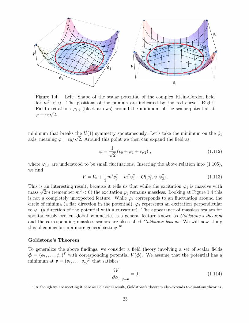
Figure 1.4: Left: Shape of the scalar potential of the complex Klein-Gordon fieldfor m2 < 0. The positions of the minima are indicated by the red curve. Right:Field excitations ϕ1,2 (black arrows) around the minimum of the scalar potential atϕ = v0

√2.

minimum that breaks the U(1) symmetry spontaneously. Let’s take the minimum on the φ1

axis, meaning ϕ = v0/√

2. Around this point we then can expand the field as

ϕ =1√2

(v0 + ϕ1 + iϕ2) , (1.112)

where ϕ1,2 are understood to be small fluctuations. Inserting the above relation into (1.105),we find

V = V0 +1

4m2v20 −m2ϕ2

1 +O(ϕ31, ϕ1ϕ

22) . (1.113)

This is an interesting result, because it tells us that while the excitation ϕ1 is massive withmass

√2m (remember m2 < 0) the excitation ϕ2 remains massless. Looking at Figure 1.4 this

is not a completely unexpected feature. While ϕ2 corresponds to an fluctuation around thecircle of minima (a flat direction in the potential), ϕ1 represents an excitation perpendicularto ϕ1 (a direction of the potential with a curvature). The appearance of massless scalars forspontaneously broken global symmetries is a general feature known as Goldstone’s theoremand the corresponding massless scalars are also called Goldstone bosons. We will now studythis phenomenon in a more general setting.10

Goldstone’s Theorem

To generalize the above findings, we consider a field theory involving a set of scalar fieldsφ = (φ1, . . . , φn)T with corresponding potential V (φ). We assume that the potential has aminimum at v = (v1, . . . , vn)T that satisfies

∂V

∂φa

∣∣∣∣φ=v

= 0 . (1.114)

10Although we are meeting it here as a classical result, Goldstone’s theorem also extends to quantum theories.

23

After defining ϕ = φ− v, we can Taylor expand the potential around such a minimum in thefollowing way

V = V (v) +1

2Mabϕ

aϕb +O(ϕ3) , (1.115)

where (a, b = 1, . . . , n)

Mab =∂2V

∂φa∂φb

∣∣∣∣φ=v

. (1.116)

Clearly, the eigenvalues of the mass matrix M are the mass squares of the fields (around thevacuum v).

Now let us assume that our scalar theory is invariant under a continuous (global) symmetrygroup G, under which

φ→ R(g)φ , (1.117)

where R(g) denotes the representation of φ. The invariance of the scalar theory in particularmeans that the scalar potential is invariant under such a transformation, namely

V (φ) = V (R−1(g)φ) , (1.118)

for all g ∈ G. The vacuum will in general not respect the full symmetry group G, but willspontaneously break it into a subgroup H ⊂ G, so that

R(g)v = v for g ∈ H , R(g)v 6= v for g 6∈ H . (1.119)

Now introducing infinitesimal group transformations

R(g) = 1 + itαTα , (1.120)

with generators Tα (in the representation R) and small coefficients tα. The set of generators{Tα} can be split into two subsets Ti and Tj, where Ti denotes the generators of the unbrokensubgroup H, while Tj are the remaining generators corresponding to the broken part of G. Bydefinition, one has

Tiv = 0 , Tjv 6= 0 . (1.121)

Now let us see how (1.120) acts on our potential. We have

V (φ) = V (φ− itαTαφ) = V (φ)− i(∂V

∂φ

)TtαTαφ . (1.122)

Differentiating this expression again and evaluating it at φ = v, one finds using (1.114)and (1.116), that

MTαv = 0 . (1.123)

From this relation we see that every broken generator Tj (with Tjv 6= 0) leads necessarily toan eigenvector of M with eigenvalue zero. Or in more physical terms, every broken symmetryleads to a massless scalar excitation. We have proven Goldstone’s theorem!

24

Scalar Field Theory With a SU(2)× U(1) Symmetry

Let us further illustrate Goldstone’s theorem by an educated example (this is a simplifiedaccount of what actually happens in the Higgs sector of the Standard Model). We considerthe symmetry SU(2)× U(1) and a complex scalar field Φ that is a doublet under SU(2) andhas a charge of 1/2 under the U(1). Our scalar transforms as

Φ→ eiαY eitiτi Φ '

(1 + iαY + itiτi

)Φ , (1.124)

with the generators

Y =1

2, τi =

σi2. (1.125)

Notice that our notation is on purpose sloppy here, since the 1 on the right-hand side of (1.124)should be in fact the 2 × 2 matrix 12. A similar statement also applies to the generator Y .Such a sloppiness in notation is common in textbooks, and it is good to get used to it early.

We can write an invariant Lagrangian as

L = (∂µΦ)† (∂µΦ)− V (Φ†Φ) (1.126)

withV (Φ†Φ) = V0 + µ2 Φ†Φ + λ

(Φ†Φ

)2. (1.127)

Provided that λ > 0 and µ2 < 0 (note we use µ2 rather than m2 for the squared mass term),the scalar potential (1.127) is bounded from below and minimized for

Φ†Φ = v20 = −µ2

2λ. (1.128)

Using (1.124) allows us to choose a particular simple vacuum configuration. Without loss ofgenerality, we take

Φ = v =

(0

v0

). (1.129)

For this choice, it is easy to verify that

τ1v 6= 0 , τ2v 6= 0 , (τ3 − Y )v 6= 0 , (1.130)

but(τ3 + Y )v = 0 . (1.131)

Hence three of the four generators of SU(2) × U(1) are broken, which corresponds to thebreaking pattern

SU(2)× U(1)→ U(1) , (1.132)

where the U(1) on the right-hand side is the diagonal subgroup of SU(2)×U(1) correspondingto the generator Q = τ3 + Y .

Although this example appears slightly contrived, its relevance stems from the fact thatthe breaking pattern (1.132) is precisely that of the electroweak gauge group of the SM of

25

particle physics: the SM is in fact based on SU(3)c × SU(2)L × U(1)Y → SU(3)c × U(1)em,where the subscript c refers to color, L indicates that the SU(2) only acts on left-handedfields, Y represents hypercharge, and U(1)em corresponds to the unbroken electromagnetismassociated to the generator Q, i.e., the electric charge.

However, there is an important difference. While the above theory predicts three masslessGoldstone bosons, in Nature we only observe a single weakly-interacting massless state, i.e.,the photon. This difference is explained by the fact that the electroweak symmetry in theSM is realized as a local or gauge(d) symmetry, while in our simple example we dealt with aglobal symmetry. It turns out that in the case of the spontaneously broken electroweak gaugesymmetry our three massless Goldstone bosons are absorbed (or eaten) by three vector bosons(the electrical neutral Z boson and the charged W± bosons) that receive their mass from thebreaking mechanism. This is the famous Higgs mechanism.

The residual massive scalar mode becomes massive is then the (physical) massive scalarstate the Higgs. After many years of searching, the Higgs boson was discovered in 2013 whenthe ATLAS and the CMS collaborations (situated at the CERN LHC in Geneva) announcedthe existence of a new bosonic state with a mass of around 125 GeV. Subsequent analyses haveshown that this particle behaves precisely as expected for a Standard Model Higgs particle.This discovery marks a turning point in the history of elementary-particle physics: the almost50 year-long hunt for the came to a successful end, and a no-lose era ended (in the sense thatthe Higgs was a guaranteed discovery for a collider that was energetic enough). The Nobelprize was then awarded to Francois Englert and Peter W. Higgs for their theoretical work onthe mechanism of electroweak symmetry breaking.

However, in order to fully understand the physics of the Higgs mechanism, we are still miss-ing an important ingredient, namely vector fields. These 4-component fields will be discussednow.

1.5 Vector Field Theories

In this section we focus on the basic features of another important ingredient of realistic(quantum) field theories, i.e., vector fields. These fields carry spin one and are called vectorfields, since they transform like a vector under the Lorentz group.

Maxwell’s Theory Of Electromagnetism

As another simple application of the formalism we have developed, let us try to deriveMaxwell’s equations using the field theory formulation. In terms of the electric and mag-netic fields E and B and the charge density ρ and 3-vector current j, these equations takethe well-known form

∇ ·B = 0 , (1.133)

∇×E +∂B

∂t= 0 , (1.134)

∇ ·E = ρ , (1.135)

26

∇×B − ∂E

∂t= j . (1.136)

The E and B fields are spatial 3-vectors and can be expressed in terms of the componentsof the 4-vector field Aµ = (φ,A) by

E = −∇φ− ∂A

∂t, B =∇×A . (1.137)

This definition ensures that the first two homogeneous Maxwell equations (1.133) and (1.134)are automatically satisfied,

∇ · (∇×A) = εijk∂i∂jAk = 0 , (1.138)

∇×(−∇φ− ∂A

∂t

)+∂

∂t(∇×A) = −∇× (∇φ) = −εijk∂j∂kφ = 0 . (1.139)

Here the indices i, j, k = 1, 2, 3 are summed over if they appear twice.The remaining two inhomogeneous Maxwell equations (1.135) and (1.136) follow from the

Lagrangian

L = −1

2(∂µAν) (∂µAν) +

1

2(∂µAν) (∂νAµ)− AµJµ , (1.140)

with Jµ = (ρ, j). From the rules presented before, we gather that the dimension of the vectorfield and current is [Aµ] = 1 and [Jµ] = 3, respectively. The funny minus sign of the first termon the right-hand side is required to ensure that the kinetic term 1/2A2

i is positive using theMinkowski metric. Notice also that the Lagrangian (1.140) has no kinetic term 1/2A2

0 andhence A0 is not dynamical. Why this is and necessarily has to be the case will become clearpretty soon.

Let us now evaluate the equations of motion and so confirm that the statement madebefore (1.140) is indeed correct. We first evaluate

∂L∂Aν

= −Jν , ∂L∂(∂µAν)

= −∂µAν + ∂νAµ , (1.141)

from which we derive the EOMs,

0 = ∂µ

(∂L

∂(∂µAν)

)− ∂L∂Aν

= ∂µ(−∂µAν + ∂νAµ) + Jν . (1.142)

Introducing now the field-strength tensor

Fµν = ∂µAν − ∂νAµ , (1.143)

we can write (1.140) and (1.142) quite compact,

L = −1

4FµνF

µν − JµAµ . (1.144)

∂µFµν = Jν , (1.145)

27

Does this look familiar? I hope so. Notice that we have [Fµν ] = 2 and that the field-strengthtensor satisfies the Bianchi identity:

∂ρFµν + ∂µFνρ + ∂νFρµ = 0 . (1.146)

In order to see that (1.145) indeed captures the physics of (1.135) and (1.136), we computethe components of F µν . We find

F 0i = −F i0 = ∂0Ai − ∂iA0 =

(∇φ+

∂A

∂t

)i= −Ei ,

F ij = −F ji = ∂iAj − ∂jAi = −εijkBk ,

(1.147)

while all other components are zero. With this in hand, we then obtain from ∂µFµ0 = ρ and

∂µFµ1 = j1,

∂µFµ0 = ∂0F

00 + ∂iFi0 =∇ ·E = ρ ,

∂µFµ1 = ∂0F

01 + ∂iFi1 = −∂E

1

∂t+∂B3

∂x2− ∂B2

∂x3=

(∇×B − ∂E

∂t

)1

= j1 .(1.148)

Similar relations hold for the remaining components i = 2, 3. Taken together this proves thesecond inhomogeneous Maxwell equation (1.136).

Let me also derive the energy-momentum tensor T µν of electrodynamics, ignoring for themoment the source term JµA

µ. Using (1.141) one finds

T µν = −F µρ∂νAρ +1

4ηµνFρσF

ρσ . (1.149)

Notice that the first term in (1.149) is not symmetric, which implies that T µν 6= T νµ. In fact,this is not really surprising since the definition of the energy-momentum tensor (1.23) doesnot exhibit an explicit symmetry in the indices µ and ν. Nevertheless, there is always a wayto massage the energy-momentum tensor of any theory into a symmetric form.11 To learn howthis can be done in the case under consideration is the objective of a homework problem.

Physical Degrees Of Freedom

Under LTs, Aµ transforms as a vector, i.e., Aµ → ΛµνAν , and the same applies of course also

to the current Jµ. The field-strength tensor Fµν , on the other hand, carries two indices andhence transforms as a tensor, i.e., Fµν → Λµ

ρΛνσFρσ. Equipped with these transformation

properties it is an easy exercise to show that the Lagrangian (1.144) is Lorentz invariant (atthe end it is sufficient to observe that in the expression for L all indices are contracted, so that(1.144) is a Lorentz scalar). The explicit calculation is left as an exercise to the interestedreader.

11One (but not the only) reason that you might want to have a symmetric energy-momentum tensor Tµν

is to make contact with general relativity, since such an object sits on the right-hand side of Einstein’s fieldequations.

28

After (1.140) we have already mentioned that not all components of Aµ are dynamical,which signals that Aµ contains unphysical dofs. In fact, this is not really a surprise becausethe physical fields E and B come from Fµν not Aµ (see (1.147)). Formally, this is expressedby the fact that a gauge transformation

Aµ(x)→ Aµ(x) + ∂µf(x) , (1.150)

with arbitrary function f(x) leaves Fµν invariant:

Fµν = ∂µAν − ∂νAµ → ∂µ(Aν + ∂νf)− ∂ν(Aµ + ∂µf)

= ∂µAν − ∂νAµ + ∂µ∂νf − ∂ν∂µf = Fµν .(1.151)

A gauge transformation should be thought of relating two physically identical configurationsfor Aµ(x).

This is an important result, because it gives us a recipe on how to “derive” the covariantformulation of electrodynamics without ever talking about Maxwell’s equations. The idea issimply to find the most general Lagrangian (including terms up to a certain mass dimension)that is Lorentz invariant and unchanged under (1.150). Notice that gauge invariance in partic-ular implies that L should only depend on Aµ through Fµν . Up to dimension four this leavesbasically only one term12 (in the case of a vanishing source term), namely L = −1/4FµνF

µν .The associated EOM is of course ∂µF

µν = 0, or written in terms of Aµ,

∂2Aµ − ∂µ∂νAν = 0 . (1.152)

In fact, this equation can be further simplified by exploiting the gauge symmetry (1.150) byimposing a gauge condition on Aµ through a suitable choice of gauge parameter f . Thereare various possibilities for such a gauge choice and here we consider the Lorenz (sic) gaugedefined by

∂µAµ = 0 . (1.153)

This gauge has the salient benefit that it is covariant (in contrast to other gauges such astemporal gauge A0 = 0 or Coloumb gauge ∇ ·A = 0) and it simplifies (1.152) to

∂2Aµ = 0 . (1.154)

It is however important to realize that (1.153) does not fix the gauge entirely but leaves aresidual gauge freedom, since all choices of f with

∂2f = 0 , (1.155)

are equivalent in the sense that they all lead to (1.154).

12The term Fµν Fµν with Fµν = εµνρσFρσ denoting the dual field-strength tensor also mets all requirements.

It can however be written as a total derivative 4∂µ(εµνρσAν∂ρAσ) and therefore does not contribute to theclassical EOMs. We hence ignore such a term.

29

The solutions of ∂2Aµ = 0 can be quickly obtained by noticing that the latter equationis nothing but a Klein-Gordon equation for a massless vector field. Adding vector indices to(1.55), we arrive at

Aµ(x) =

∫d3p

(2π)31

2ωp

(aµ(p)e−ipx + a∗µ(p)eipx

), (1.156)

where ωp = |p| and pµ = (ωp,p). After a Fourier transform, the Lorenz gauge condition(1.153) can be written as

pµaµ(p) = 0 . (1.157)

This gauge condition can be used to show that there are only two physical degrees offreedom in the electromagnetic field - the polarisation modes transverse to the direction ofpropagation. This result should be familiar to you from the study of sunglasses, and we nowsee how it arises here.

To exploit this constraint one conveniently introduces a set of polarization vectors ε(α)µ (p)

with α = 0, 1, 2, 3 and the following properties. The vectors ε(1)µ and ε

(2)µ are orthogonal to

both p and a vector n with n2 = 1 and n0 > 0. They furthermore are chosen such that theysatisfy ε(α) · ε(β) = −δαβ for α, β = 1, 2. The polarization vector ε

(3)µ is taken to be in the p–n

plane, orthogonal to n and normalized to -1, i.e., n · ε(3) = 0 and (ε(3))2 = −1. Finally, onedefines ε(0) = n. With these conventions one has an orthogonal set of vectors satisfying

ε(α) · ε(β) = ηαβ , (1.158)

for α, β = 0, 1, 2, 3. This basis can be used to write

aµ(p) =3∑

α=0

a(α)(p)ε(α)µ (p) . (1.159)

In fact, the basic idea behind all this “mumbo-jumbo” is that this specific choice of basis ofpolarization vectors, allows to easily separate the directions transversal to p (corresponding to

ε(1)µ and ε

(2)µ ) from the other two directions (corresponding to ε

(0)µ and ε

(3)µ ) that are longitudinal

to p. As an example, if we choose a spatial momentum p pointing in the z-directions, thecomponents of above vectors are explicitly given by

ε(α)µ = δαµ . (1.160)

In the general case, one has instead

ε(3)µ =pµp0− nµ . (1.161)

Clearly,

n · ε(3) =np

p0− n2 =

np

p0− 1 = 0 =⇒ np

p0= 1 , (1.162)

and thus

(ε(3))2 =p2

p20+ n2 − 2

np

p0= 1− 2

np

p0= −1 , (1.163)

30

where we have used that our vector field is massless, i.e., p2 = 0. So (1.161) is indeed thesought solution. Notice also that

ε(0)µ + ε(3)µ =pµp0. (1.164)

We now return to (1.157) and evaluate this sum inserting the expansion (1.159). By

definition the transversal components ε(1)µ and ε

(2)µ do not contribute and we find

pµaµ(p) = (p · ε(0))a(0)(p) + (p · ε(3))a(3)(p) = p0(a(0)(p)− a(3)(p)

)= 0 . (1.165)

Here we have used thatp · ε(0) = −p · ε(3) = p0 . (1.166)

Note that the first equality follows from (1.164) after contracting it with pµ, while the secondequality is a consequence of (1.162). From (1.165) it follows that a(0)(p) = a(3)(p). Theexpansion (1.159) can thus be written as

aµ(p) = a(3)(p)pµp0

+2∑

α=1

a(α)(p)ε(α)µ (p) , (1.167)

and we are left with two transversal modes and a longitudinal one along the p direction(remember that after (1.140) we already mentioned the fact that the time component A0 isnot dynamical, which reduces the number of independent dofs in Aµ from four to three). Thisis still one more dof than a physical massless field, such as the photon, ought to have.

The trick to get rid of the remaining longitudinal component is to make use of the residualgauge freedom (1.155) and to “gauge away” the term proportional to a(3)(p) in (1.167). Letsee how this works. Given that f also fulfils a Klein-Gordon equation, the most generaldecomposition obviously reads

f(x) =

∫d3p

(2π)31

2ωp

(ξ(p)e−ipx + ξ∗(p)eipx

). (1.168)

A gauge transformation (1.150) with such a f corresponds to

aµ(p)→ a′µ(p) = aµ(p)− ipµξ(p) . (1.169)

But such a shift is exactly what is needed to remove the remaining longitudinal componentfrom (1.167) and we arrive at the correct physical answer. Needless to say that the reduc-tion from apparent four dofs to actually two is intimately related to the gauge invariance of(quantum) electrodynamics.13

A Massive Vector Field

What happens if we try to give our vector field Aµ a mass? We can try and add a term

1

2m2AµA

µ , (1.170)

13Although we have presented a classical argument, an analogous argument also holds in the quantum theory.

31

to our Lagrangian L = −1/4FµνFµν , but immediately realize that such a term is not allowed

by gauge invariance (1.150). This is of course stupid, but let us ignore this unwanted featurefor a moment. The EOMs for the massive vector field would not be ∂µF

µν = 0, but

∂µFµν +m2Aν = 0 . (1.171)

Applying ∂ν to this relation we conclude that ∂νAν = 0, since ∂ν∂µF

µν is trivially zero. Wecan hence split the latter equation into two

(∂2 +m2)Aµ = 0 , ∂µAµ = 0 . (1.172)

The first equation is a massive Klein-Gordon equation for Aµ with the general solution (1.156)but ωp = (|p|2 + m2)1/2 instead of ωp = |p|. In order to satisfy the second equation we needto impose the condition (1.157), which reduces the number of dofs from four to three. Can wescrap another dof? Not this time - the mass term (1.170) breaks gauge invariance and thus wedo not have the freedom to use (1.155) and gauge it away. This means that a massive vectorfield has three physical degrees of freedom, one more than a massless one.

Current Sources

In the discussion of the last two subsections we have always ignored the possible presenceof external sources by simply setting Jµ = 0 by hand. If we now include a source term,the relevant Lagrangian leading to Maxwell’s theory has already been given in (1.144). Byapplying (1.150), we see that a gauge transformation of such a term introduces an additionalpiece into the action:

S → S −∫d4x (∂µf) Jµ = S +

∫d4x f (∂µJ

µ) . (1.173)

As usual we have used integration by parts to arrive at the final answer. This result tells usthat the apparent breaking of gauge invariance by the term JµA

µ can be avoided, providedthat

∂µJµ = 0 . (1.174)

In other words, the vector field Aµ needs to couple to a conserved current Jµ. In a fundamentaltheory, we expect the current Jµ to itself arise from fields, rather than simply being put in byhand as an external source.

We now conclude the chapter on classical field theory by studying the simplest fundamentaltheory of such a kind.

Scalar Electrodynamics And Abelian Higgs Mechanism

The goal of this final subsection is to write down an interesting theory involving a complexscalar ϕ and a vector field Aµ. ’Interesting’ is defined to mean that the two fields interact,which requires a Lagrangian involving terms with both ϕ and Aµ. The problem is now that ingeneral ϕ and Aµ do not transform trivially under a given symmetry. E.g., the complex scalarϕ transforms as (1.103) under a global U(1), while Aµ obeys the gauge transformation (1.150).

32

The important point to notice is that both transformations involve only a single parameter,namely α and f . However, α = const. is space-time independent, while f = f(x) is a functionof the space-time coordinate x. What happens if we generalize (1.103) by allowing the U(1)symmetry to be local rather than global? Our fields ϕ and ϕ∗ then transform as

ϕ→ ϕ′ = eiα(x)ϕ , ϕ∗ → (ϕ′)∗ = e−iα(x)ϕ∗ . (1.175)

Since the scalar potential is polynomial in ϕ∗ϕ it is clearly invariant under these local U(1)transformations. But as already noted after (1.105), for the kinetic term to be invariant, weneeded α = const. Explicitly, we have

∂µϕ→ ∂µ(eiα(x)ϕ

)= eiα(x) (∂µ + i∂µα(x))ϕ . (1.176)

Obviously, the term involving ∂µα(x) will cause (∂µϕ∗)(∂µϕ) to transform non-trivially un-

der (1.175). However, we still have the gauge transformation (1.150) of the vector field, whichalso involves a term with a derivative. So let us see how (∂µ − iAµ)ϕ transforms. One finds

(∂µ − iAµ)ϕ→ eiα [(∂µ + i∂µα)− i(Aµ + ∂µf)]ϕ = eiα [(∂µ − iAµ) + i∂µ(α− f)]ϕ . (1.177)

This prompts us to realise that if we identify α(x) = f(x) then

Dµϕ = (∂µ − iAµ)ϕ , (1.178)

has the correct properties! It transforms as

(Dµϕ)∗(Dµϕ)→ (Dµϕ)∗(Dµϕ) , (1.179)

underϕ→ eiαϕ , Aµ → Aµ + ∂µα . (1.180)

In other words the new kinetic term (Dµϕ)∗(Dµϕ), with ∂µ replaced by the covariant derivativeDµ, is gauge invariant. Notice that the covariant derivative (1.178) has dimension [Dµ] = 1and involves a “minimal” coupling Aµϕ between the vector field Aµ and the scalar ϕ.

We can now combine our scalar and gauge field Lagrangian to obtain

L = (Dµϕ)∗(Dµϕ)− V (ϕ∗ϕ)− 1

4FµνF

µν , V (ϕ∗ϕ) = V0 +m2ϕ∗ϕ+λ

4(ϕ∗ϕ)2 , (1.181)

which is the Lagrangian of scalar electrodynamics - describing a charged complex scalar coupledto electromagnetism. Notice that in this new theory the role of Aµ is to facilitate the invarianceof the scalar field theory under local gauge transformations. In fact, if we would have startedfrom the global U(1) invariant scalar theory, with the task of finding its locally U(1) invariantversion, we would have necessarily been led to introducing a gauge field Aµ.

We will now use (1.181) as a toy model to study the spontaneous symmetry breaking of alocal U(1) symmetry. Since the scalar potential is identical to the one in the global case, wecan reuse all our old results. The case m2 ≥ 0 is again not very interesting since the symmetryis unbroken, so let’s focus on the situation with m2 < 0. In the latter case the potential takes

33

the form of a “Mexican hat” as in Figure 1.4. We parametrize ϕ around the minima in thefollowing way

ϕ =1√2

(v0 + h) eiχ , (1.182)

with v0 given in (1.110). It is straightforward to see that h corresponds to a real massive field,while χ is a Goldstone mode (also a real field). We can now eliminate the Goldstone modefrom ϕ by choosing the specific gauge

ϕ→ ϕ′ = e−iχϕ =1√2

(v0 + h) . (1.183)

Under this transformation, we see from (1.180) that

Aµ → A′µ = Aµ − ∂µχ . (1.184)

Since the Lagrangian (1.181) is gauge invariant, we can as well write it in terms of primedrather than unprimed fields. For the covariant derivative, one finds

(Dµϕ)′ =1√2

(∂µh− i (v0 + h)A′µ

), (1.185)

and inserting this expression into (1.181) leads to

L =1

2(∂µh)2 +

1

2A′µA

′µ (v20 + 2v0h+ h2)− V (h)− 1

4F ′µνF

′µν , (1.186)

with

V (h) = V0 +1

4m2v20 −m2h2 +

λ

16

(4v0h

3 + h4). (1.187)

The most striking feature of this result is that the Goldstone mode χ has (magically) disap-peared and we are only left with the fields h and A′µ. So did we loose a dof? No, because thevector field is now no longer massless, but has a mass

mA′ = v0 . (1.188)

It has hence three dofs (as opposed to just two in the massless case), which explains thedisappearance of χ: the Goldstone boson has been “eaten” by the vector field and providesthe additional longitudinal component for the massive A′µ. This feature can also be inferredfrom (1.184). Notice furthermore that the mass of h is given by

mh =√−2m2 , (1.189)

and that (1.186) and (1.187) have a rich structure of interactions: there are couplings of twogauge fields to one and two massive scalars (A′A′h and A′A′h2) as well as cubic and quarticself-couplings of the massive scalar (h3 and h4).

So let’s briefly summarize our main findings: we have learned that a spontaneously brokenlocal (or gauge) symmetry leads to a mass for the associated vector boson and the conversion

34

of the Goldstone boson into the longitudinal component of the gauge field. This is the famousHiggs mechanism that we already alluded to.

The Higgs mechanism had already appeared within superconductivity. This can be un-derstood as the spontaneous breaking of electromagnetism within a superconductor, so thatthe photon is effectively massive and the magnetic field is expelled from the interior of thesuperconductor.

The massive scalar h left over in our model is called the Higgs scalar. The phenomenondescribed above (but in its generalization to non-abelian gauge groups) is at work in the SMof particle physics. In fact, since the SM symmetry breaking pattern is SU(2)L × U(1)Y →U(1)em, there are three Goldstone bosons that give masses to three electroweak gauge bosons.The masses of these particles are all proportional to the symmetry breaking scale (or vacuumexpectation value) v0. A detailed discussion of the breaking of the electroweak symmetry, whileworthwhile, is beyond the scope of this lecture, as it requires the introduction of non-abeliangauge symmetries, but you will learn a bit more in one of the exercises.

35