Intensive Computation

Annalisa Massini

The course will cover topics that are in some sense

related to intensive computation:

• Matlab (an introduction)

• GPU (an introduction)

• Sparse matrices

• Eigenvectors and eigenvalues, graph connectivity

• Molecular Dynamics

• Global search: simulated annealing, tabu search, …

• IEEE floating point representation and arithmetic

• Errors

• Simulations

Course topics

- 25th March lecture will be given by Paolo D'Onorio De

Meo and Mattia D’Antonio on Apache Hadoop, an open-

source software framework for storage and large scale

processing of data-sets on clusters (for bioinformatics)

- Exam project (or master thesis) on Hadoop

Course page is

http://twiki.di.uniroma1.it/twiki/view/CI/WebHome

Course topics

- Aula Alfa is reserved Tuesdays and Fridays, 12:00 to 13:30

- the course requires a quantity of hand-on work

- we will have lectures and laboratory classes

- Colossus Laboratory Tuesdays or Fridays, 12:00 to 13:30,

according to the previous lecture

Lectures will be given by using slides or by using the

blackboard

Time and venue

- Exercises will be assigned during the course

- Exercises are due during the week for intermediate exam

and during the course final week

- The presentation of a project developed with Matlab (or

on GPU) on one of the course topics

There is not a book – I will give you slides and references

on the topics of the course

Exam

Introduction Traditional methods in science and engineering are:

To develop theories and projects

To execute experiments and to build systems

These tasks can be :

Too difficult -------- wind tunnel

Too expensive ---- crash testing

Too slow ------------ the evolution of a galaxy

Too dangerous --- drugs, toxic gas diffusion

Introduction Computers represent the fundamental tool for the

simulation and can be seen both as a microscope and

as a telescope with respect to space and to the time

Examples:

To model molecules in details

To travel to the origin of the universe and study its evolution

To provide weather forecasts or climate changes

Introduction Instruments as particle accelerator, telescopes, scanner,

etc., produce big quantity of data

The obtained data are elaborated by means of a computer

and are:

Reduced and transformed

Represented and visualized

Objectives of data elaboration are:

To understand the meaning of the produced data

To develop new theories

To verify different kind of phenomena

Computational Science Computational science is concerned with constructing

mathematical models

quantitative analysis techniques

using computers

to analyze and solve scientific problems

Computational science involves the application of computer

simulation and other forms of computation, from numerical

analysis and theoretical computer science, to problems in

various scientific disciplines.

Computational Science The scientific computing approach is to gain understanding,

mainly through the analysis of mathematical models

implemented on computers.

Computational science is different from theory and

laboratory experiments, which are the traditional forms of

science and engineering.

Computational science is now considered a third mode

of science, besides experimentation/observation and

theory.

Computational Science Scientists and engineers develop computer programs

and application software, that model systems being

studied.

These programs are run with various sets of input

parameters.

In some cases, these models require massive amounts

of calculations (usually floating-point numbers) that are

executed on supercomputers or distributed computing

systems.

Grand challenges Grand Challenges were USA policy terms set as goals

in the late 1980s for funding high-performance computing and communications research

"A Research and Development Strategy for High Performance Computing", Executive Office of the President, Office of Science and Technology Policy, November 20, 1987

"A grand challenge is a fundamental problem in science or engineering, with broad applications, whose solution would be enabled by the application of high performance computing resources that could become available in the near future."

Grand challenges 1. Computational fluid dynamics for

the design of hypersonic aircraft, efficient automobile bodies, and

extremely quiet submarines

weather forecasting for short and long term effects

efficient recovery of oil, and for many other applications

2. Electronic structure calculations for the design of new

materials such as

chemical catalysts

immunological agents

superconductors

3. Plasma dynamics for fusion energy technology and

for safe and efficient military technology

4. Calculations to understand the fundamental nature of

matter, including quantum chromodynamics and

condensed matter theory

5. Symbolic computations including speech recognition speech recognition

computer vision

natural language understanding

automated reasoning

tools for design, manufacturing, and simulation of complex systems

Grand challenges

21st Century Grand Challenges

On April 2, 2013, President Obama called on companies,

research universities, foundations, and philanthropists to

join him in identifying and pursuing the Grand Challenges

of the 21st century.

Grand Challenges are ambitious but achievable goals that

harness science, technology, and innovation to solve

important national or global problems and that have the

potential to capture the public’s imagination.

Greenhouse effect simulation

As an example we describe an experiment done in the late

’90s for studying global warming a problem that is still

studied and has been the subject of international attention.

This problem is studied by computer simulations to

understand how changing concentrations of carbon

dioxide in the atmosphere contribute to global warming

through the greenhouse effect.

A study of this type requires modeling the climate over a

long period of time.

The climate model known as the General Circulation Model,

GCM, was used by the National Center for Atmospheric

Research to study the warming which would be caused by

doubling the concentration of carbon dioxide over a period

of 20 years.

The computations were done on a Cray-1, with a peak

speed of about 200 Mflops (2x102x106 flops/s):

110 s per simulated day

Two 19-year simulations required 400 computational

hours

Now a desktop processor peak speed is about 70 gflops (Intel i7)

Greenhouse effect simulation

The effects that the GCM attempts to

model are:

The atmosphere is a fluid the

behaviour of fluids is described by

partial differential equations

Computer solution of these equations is

obtained by means of the finite difference

algorithm in which derivatives with respect

to spatial coordinates and time are

approximated by difference formulas.

Greenhouse effect simulation

A 3D mesh in space is

considered

The mesh used in the

computations was composed

by about 2000 points to

cover the surface of the

earth and 9 layers of

different altitudes

There are 8-9 variables at

each mesh point that must

be updated (temperature,

CO2 concentration, wind

velocity, etc).

Computer performance is

very important!!

Greenhouse effect simulation

Solution of the problem needs a set of initial conditions for

which values are assigned to the variables at each mesh

point and stepping forward in time updating these variables

at the end of each step

Observation The mesh is extremely coarse!!

Infact the surface of the earth is 5,1 x 108 km2 one mesh

point over an area 2,6 x 105 km2, that is on a land area like

Spain-Portugal there are 2 mesh points!

Greenhouse effect simulation

We would like to have a greater accuracy, that is more

mesh points

If we double the density of points in each of the three

directions:

we increase the number of mesh points of a factor of 8

the computation that took 400 hours in this case would

take over 3000 hours, but we still have only few points

on Spain-Portugal

Greenhouse effect simulation

General Strategy

When we define a solution for a computational problem, the

general strategy is :

To substitute a difficult problem by an easier problem

with the same solution or solution quite similar

To this end we can

substitute infinite spaces with spaces of finite dimension

substitute infinite processes with finite processes, for

example we can substitute integrals or infinite series with

finite sums or we can substitute derivatives with finite

differences

General Strategy

…

substitute differential equations with algebraic equations

substitute non linear problems with linear problems

substitute higher degree problems with lower degree

problems

substitute difficult functions with simpler function, such as

polynomials

substitute general matrices with simpler matrices

At each step it is needed to verify that the solution doesn’t change or it changes within a certain threshold with respect to real solution

Example

To solve a system of nonlinear differential equations we

can:

Substitute the system of differential equations with a

system of algebraic equations

Substitute the nonlinear algebraic system with a

linear system

Substitute the matrix of the linear system with a

matrix with a simpler solution to compute

General Strategy

To make the general strategy appliable, we need:

A problem or a class of problems easier to solve

A transformation from the given problem to the

simplified problem that preserve the solution

If the solution of the new problem (the transformed

problem) is an approximation of the real solution, then we

have to estimate the accuracy and to compute the

convergence toward the real solution

The accuracy can be made as good as we want by using

time consuming and memory consuming computations

Simulations Computer simulation has become an important part of

modeling

natural systems in physics, chemistry and biology

human systems in economics and social science

engineering to gain insight into the operation of systems

Typical problems:

Handle big quantity of data

Consider scale with very small or huge values for distances

and time (molecules, astronomy)

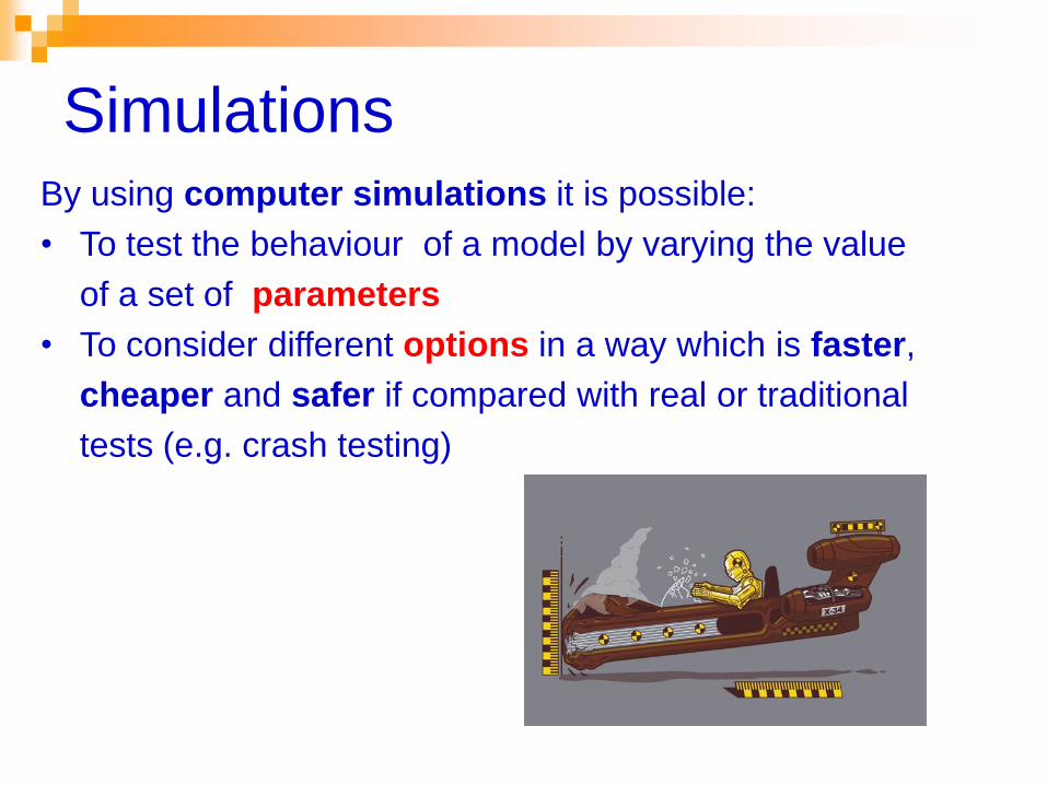
Simulations By using computer simulations it is possible:

• To test the behaviour of a model by varying the value

of a set of parameters

• To consider different options in a way which is faster,

cheaper and safer if compared with real or traditional

tests (e.g. crash testing)

Solutions e simulations

The solution of a problem by means of computational

simulations requires a sequence of steps:

1. To develop a mathematical model, consisting of

equations describing the physical system or phenomenon

of interest

2. To develop algorithms to numerically solve the equations

of the mathematical model

3. To implement the algorithms with a suitable language or

in a suitable sw environment

Solutions e simulations

4. To run programs on a high performance computer

selected for the specific problem

5. To represent computed data using a graphical

visualization that makes them understandable

6. To validate and to interpretate the obtained results, and to

repeate some of the previous steps

Note that in this process each step influences and is

influenced by the other steps.

Solutions e simulations

A problem is said well-posed if a solution exists, the

solution is unique and it continuously changes with the

initial conditions.

Continuum models must often be discretized in order to

obtain a numerical solution.

While solutions may be continuous with respect to the initial

conditions, they may suffer from numerical instability when

solved with finite precision or with errors in the data.

Solutions e simulations

Even if a problem is well-posed, it may still be ill-

conditioned, meaning that a small error in the initial data

can result in much larger errors in the solution.

If the problem is well-posed, then it stands a good chance

of solution on a computer using a stable algorithm.

If it is not well-posed, it needs to be re-formulated for

numerical treatment. Typically this involves including

additional assumptions, such as smoothness of solution.

Solutions e simulations

Problems that are not well-posed are termed ill-posed.

Inverse problems are often ill-posed.

For example, the inverse heat equation, deducing a

previous distribution of temperature from final data, is not

well-posed in that the solution is highly sensitive to changes

in the final data.

Another example is the study of internal structure of a

physical system from an external observation, as in the

case of tomography or in seismology. Often the derived

problems are ill-posed because very different configurations

can assume the same external appearance.

High performance computing

High Performance Computing (HPC) generally refers to

the practice of aggregating computing power to deliver

higher performance with respect to a typical desktop

computer or workstation

HPC is used to solve large problems in science,

engineering, or business

HPC tasks are characterized as needing large amounts of

computing power

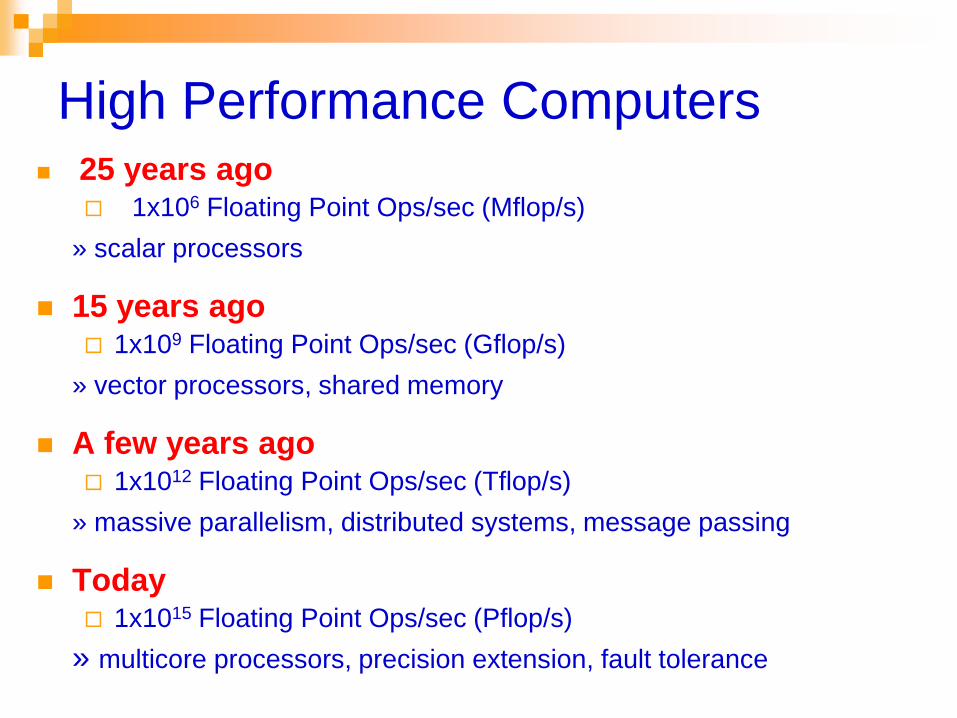
High Performance Computers 25 years ago

1x106 Floating Point Ops/sec (Mflop/s)

» scalar processors

15 years ago 1x109 Floating Point Ops/sec (Gflop/s)

» vector processors, shared memory

A few years ago 1x1012 Floating Point Ops/sec (Tflop/s)

» massive parallelism, distributed systems, message passing

Today 1x1015 Floating Point Ops/sec (Pflop/s)

» multicore processors, precision extension, fault tolerance

GPU and GPGPU

GPU, Graphics Processing Unit, is a specialized

electronic circuit designed to rapidly manipulate computer

graphics and to render 3D images

GPGPU (General Purpose computing on GPU) is the

utilization of a GPU to perform computation in applications

traditionally handled by CPU

The highly parallel structure of GPUs makes them more

effective than general-purpose CPUs for algorithms where

processing of large blocks of data is done in parallel

35

Some of the areas where GPUs have been used for general

purpose computing are:

● Weather forecasting

● Molecular dynamics

● Computational finance

● Protein alignment and genoma project

36

GPU and GPGPU

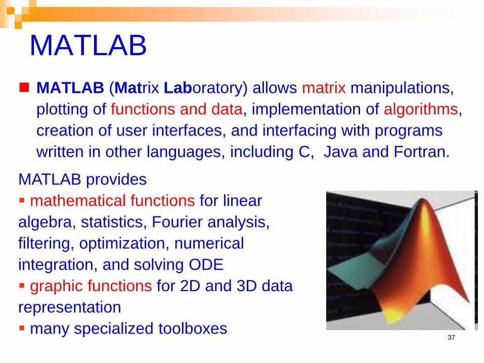
MATLAB

MATLAB (Matrix Laboratory) allows matrix manipulations,

plotting of functions and data, implementation of algorithms,

creation of user interfaces, and interfacing with programs

written in other languages, including C, Java and Fortran.

37

MATLAB provides

mathematical functions for linear

algebra, statistics, Fourier analysis,

filtering, optimization, numerical

integration, and solving ODE

graphic functions for 2D and 3D data

representation

many specialized toolboxes