i

ELEMENTARY SCHOOL TEACHERS' UNDERSTANDING OF ESSENTIAL TOPICS IN STATISTICS AND THE INFLUENCE OF ASSESSMENT

INSTRUMENTS AND A REFORM CURRICULUM UPON THEIR UNDERSTANDING

A Dissertation Presented to

the Graduate School of Clemson University

In Partial Fulfillment of the Requirements for the Degree

Doctor of Philosophy Curriculum and Instruction

by Tim Jacobbe August 2007

Accepted by: Dr. Bob Horton, Committee Chair

Dr. Donna Diaz Dr. Elizabeth Edmondson Dr. Suzanne Rosenblith

Timothy Jacobbe - Elementary school teachers’ understanding of essential topics in statistics and the influence of assessmentinstruments and a reform curriculum upon their understanding

ii

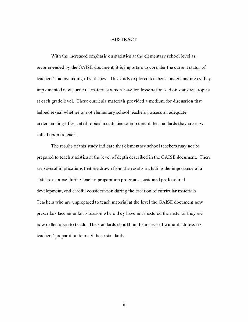
ABSTRACT

With the increased emphasis on statistics at the elementary school level as

recommended by the GAISE document, it is important to consider the current status of

teachers� understanding of statistics. This study explored teachers� understanding as they

implemented new curricula materials which have ten lessons focused on statistical topics

at each grade level. These curricula materials provided a medium for discussion that

helped reveal whether or not elementary school teachers possess an adequate

understanding of essential topics in statistics to implement the standards they are now

called upon to teach.

The results of this study indicate that elementary school teachers may not be

prepared to teach statistics at the level of depth described in the GAISE document. There

are several implications that are drawn from the results including the importance of a

statistics course during teacher preparation programs, sustained professional

development, and careful consideration during the creation of curricular materials.

Teachers who are unprepared to teach material at the level the GAISE document now

prescribes face an unfair situation where they have not mastered the material they are

now called upon to teach. The standards should not be increased without addressing

teachers� preparation to meet those standards.

iii

DEDICATION

This dissertation is dedicated to my loving wife Elizabeth and our two wonderful

children, Hannah and Nathan. Without Elizabeth�s patience, support, understanding, and

love, I would not have had the time and energy to complete this project. Hannah and

Nathan have patiently awaited the completion of this dissertation and are looking forward

to more play time with Daddy. The completion of this program would not be as fulfilling

if it were not for the happiness they bring to my life.

iv

ACKNOWLEDGMENTS

This dissertation could not have been written without Dr. Bob Horton who not

only served as my advisor but also encouraged and challenged me throughout my

academic program. He and the other members of my committee, Dr. Donna Diaz, Dr.

Elizabeth Edmondson, and Dr. Suzanne Rosenblith guided me through the dissertation

process. In addition to constructive feedback, Dr. Donna Diaz provided me support and

encouragement throughout the process.

I would like to thank Dr. Bill Moss and Dot Moss who provided support for my

entire family while going through the final stages of the dissertation process. I would

also like to thank my brother, Mike, and his wife, Julie, who provided tremendous

support for my family. Their support provided comfort during a difficult time of

transition.

In addition, my colleagues at Educational Testing Service provided support

during the research process. In particular, Dr. David Banach and Jeff Haberstroh

provided insight and guidance during the data collection process. Through my

interactions with various programs with Educational Testing Service, I had the honor of

working with Dr. Chris Franklin, Dr. Brad Hartlaub, and Dr. Calvin Williams. They

provided support and guidance whenever I had questions.

Finally, I cannot thank Dr. Barbara Moses enough for sparking my interest in

mathematics education. I would not have reached this point in my career without the

influence of Dr. Moses. She not only served as my advisor during undergraduate and

graduate studies at Bowling Green State University, but she has become a lifelong friend.

v

TABLE OF CONTENTS

Page

TITLE PAGE ............................................................................................................... i ABSTRACT................................................................................................................ ii DEDICATION........................................................................................................... iii ACKNOWLEDGMENTS .......................................................................................... iv LIST OF TABLES ................................................................................................... viii LIST OF FIGURES.................................................................................................... ix CHAPTER I. INTRODUCTION ..................................................................................... 1 Statistics in the K-12 Setting ................................................................ 3 Problematizing Teachers� Awareness of their Understanding .................................................................................. 7 Purpose of This Study .......................................................................... 9 Research Questions .............................................................................. 9 II. REVIEW OF THE LITERATURE ...........................................................10 What Do the Standards Say? ...............................................................10 The GAISE Document ........................................................................12 Research Related to Statistics in the Elementary School .............................................................................................21 Content Knowledge.............................................................................24 III. METHOD.................................................................................................33 Setting.................................................................................................34 Qualitative Design, Role of Researcher, and Participants....................................................................................35 Math Out of the Box Materials.............................................................40 Three Phases of Data Collection..........................................................43 Methods of Verification ......................................................................49 Limitations..........................................................................................50

vi

Table of Contents (Continued)

Page IV. ANALYSIS AND RESULTS ...................................................................53 Categorization of the Questions...........................................................53 Teachers� Performance in the Area of Data Displays ........................................................................................57 Teachers� Performance in the Area of Measures of Central Tendency.......................................................78 Teachers� Performance in the Area of Measures of Variation .................................................................103 Connecting the Teachers� Understanding of The GAISE..................................................................................113 Teachers� Awareness of their Understanding.....................................116 V. IMPLICATIONS ....................................................................................121 Answering the Research Questions....................................................121 Procedural versus Conceptual Knowledge of Essential Topics in Statistics........................................................122 Implications for Teacher Training .....................................................128 Sustained Professional Development Experiences .............................130 Implications for Curricular Development...........................................131 Areas for Future Research .................................................................134 APPENDICES .........................................................................................................138 A: Baseline Teacher Interview Protocol .......................................................139 B: Observational Protocol............................................................................141 C: Statistical Content Interview ...................................................................142 D: Math Out of the Box Interview ................................................................144 E: Assessment 1 (NAEP Items 4th Grade Level) Used by ETS to assess Content Knowledge of Students......................................................................145 F: Assessment 2 (NAEP Items 4th Grade Level) Used by ETS to assess Content Knowledge of Students......................................................................151 G: Selected Statistical Items from University Of Louisville .....................................................................................158

vii

Table of Contents (Continued)

Page H: Content Knowledge Assessments Using Center and Variation to Make Decisions (From 2006 AP Statistics Exam) ......................................................164 I: Card Sorting Tasks..................................................................................166 REFERENCES.........................................................................................................168

viii

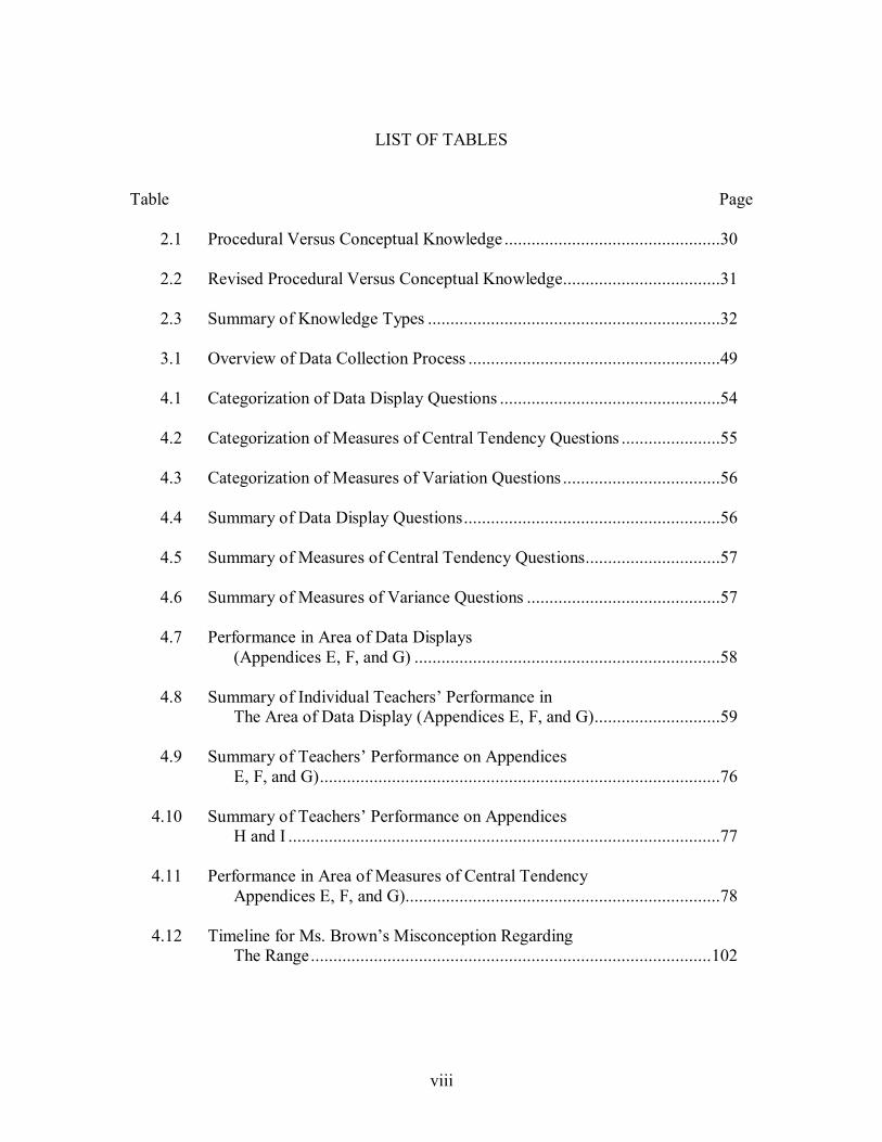
LIST OF TABLES

Table Page 2.1 Procedural Versus Conceptual Knowledge ................................................30 2.2 Revised Procedural Versus Conceptual Knowledge...................................31 2.3 Summary of Knowledge Types .................................................................32 3.1 Overview of Data Collection Process ........................................................49 4.1 Categorization of Data Display Questions .................................................54 4.2 Categorization of Measures of Central Tendency Questions ......................55 4.3 Categorization of Measures of Variation Questions ...................................56 4.4 Summary of Data Display Questions.........................................................56 4.5 Summary of Measures of Central Tendency Questions..............................57 4.6 Summary of Measures of Variance Questions ...........................................57 4.7 Performance in Area of Data Displays (Appendices E, F, and G) ....................................................................58 4.8 Summary of Individual Teachers� Performance in The Area of Data Display (Appendices E, F, and G)............................59 4.9 Summary of Teachers� Performance on Appendices E, F, and G).........................................................................................76 4.10 Summary of Teachers� Performance on Appendices H and I ................................................................................................77 4.11 Performance in Area of Measures of Central Tendency Appendices E, F, and G)......................................................................78 4.12 Timeline for Ms. Brown�s Misconception Regarding The Range.........................................................................................102

ix

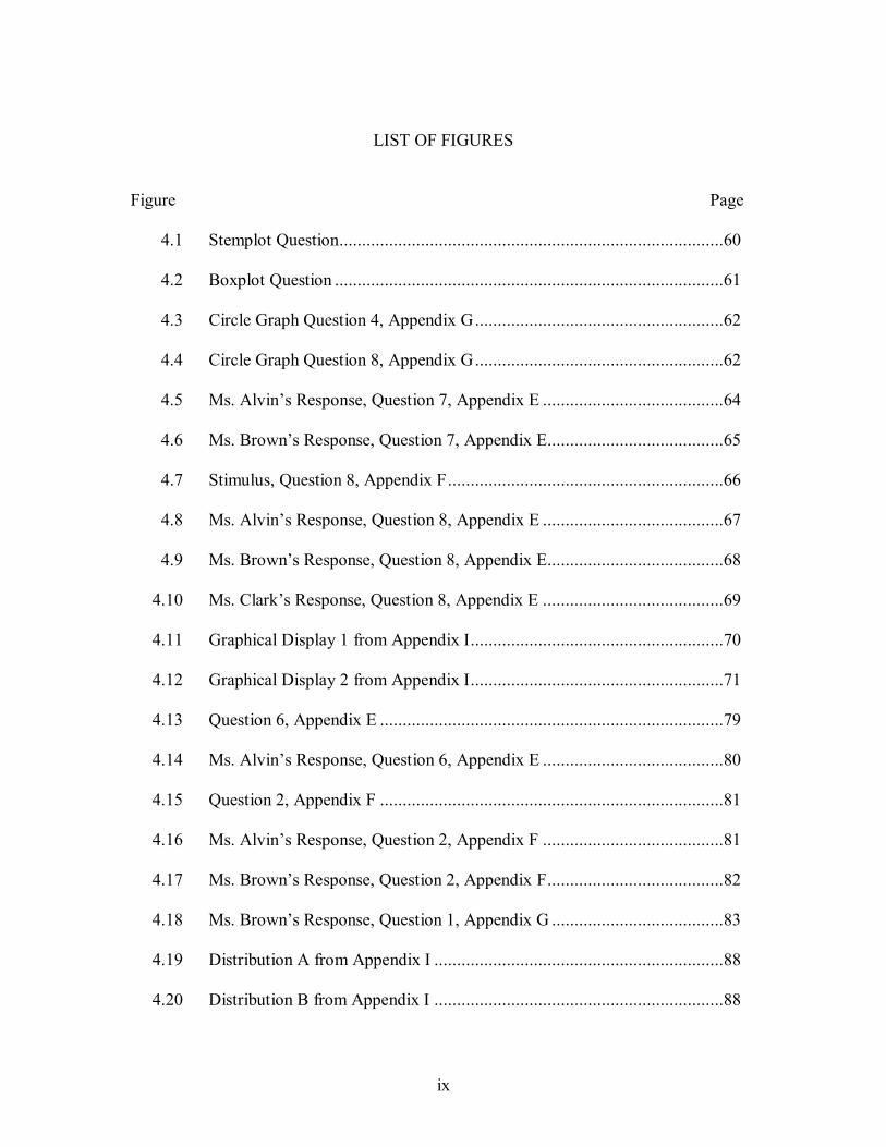
LIST OF FIGURES

Figure Page 4.1 Stemplot Question.....................................................................................60 4.2 Boxplot Question ......................................................................................61 4.3 Circle Graph Question 4, Appendix G.......................................................62 4.4 Circle Graph Question 8, Appendix G.......................................................62 4.5 Ms. Alvin�s Response, Question 7, Appendix E ........................................64 4.6 Ms. Brown�s Response, Question 7, Appendix E.......................................65 4.7 Stimulus, Question 8, Appendix F.............................................................66 4.8 Ms. Alvin�s Response, Question 8, Appendix E ........................................67 4.9 Ms. Brown�s Response, Question 8, Appendix E.......................................68 4.10 Ms. Clark�s Response, Question 8, Appendix E ........................................69 4.11 Graphical Display 1 from Appendix I........................................................70 4.12 Graphical Display 2 from Appendix I........................................................71 4.13 Question 6, Appendix E ............................................................................79 4.14 Ms. Alvin�s Response, Question 6, Appendix E ........................................80 4.15 Question 2, Appendix F ............................................................................81 4.16 Ms. Alvin�s Response, Question 2, Appendix F ........................................81 4.17 Ms. Brown�s Response, Question 2, Appendix F.......................................82 4.18 Ms. Brown�s Response, Question 1, Appendix G ......................................83 4.19 Distribution A from Appendix I ................................................................88 4.20 Distribution B from Appendix I ................................................................88

x

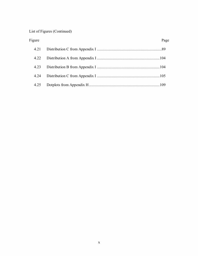
List of Figures (Continued) Figure Page 4.21 Distribution C from Appendix I ................................................................89 4.22 Distribution A from Appendix I ..............................................................104 4.23 Distribution B from Appendix I ..............................................................104 4.24 Distribution C from Appendix I ..............................................................105 4.25 Dotplots from Appendix H......................................................................109

1

CHAPTER ONE

INTRODUCTION

Based on the groundbreaking efforts of the Quantitative Literacy Project

(Schaeffer, 1986), the National Council of Teachers of Mathematics (NCTM) has

gradually increased the depth of statistical topics covered in elementary, middle, and

secondary schools (1989, 2000). The Data Analysis and Probability Standard in the

Principles and Standards for School Mathematics (NCTM, 2000) encourages

instructional programs from prekindergarten through grade 12 [that] enable all students

to:

• formulate questions that can be addressed with data and collect, organize, and

display relevant data to answer them; • select and use appropriate statistical methods to analyze data;

• develop and evaluate inferences and predictions that are based on data; AND

• understand and apply basic concepts of probability. (NCTM, 2000, p. 48)

In order to support the objectives set forth in the Principles and Standards for

School Mathematics, the American Statistical Association released a curriculum

framework for PreK-12 Statistics Education known as the Guidelines for Assessment and

Instruction of Statistics Education (GAISE) (Franklin et. al., 2005). �This Framework

provides a conceptual structure for statistics education which gives a coherent picture of

the overall curriculum. This structure adds to but does not replace the NCTM

recommendations� (Franklin et al., 2005, p. 5).

2

The GAISE suggests an increase in the level of sophistication for the teaching and

learning of statistics in K-12 classrooms. The authors indicate �a major objective of

statistics education is to help students develop statistical thinking. Statistical thinking, in

large part, must deal with the omnipresence of variability; statistical problem solving and

decision making depend on understanding, explaining and quantifying the variability in

the data� (Franklin et. al., 2005, p.5). The goals set forth by NCTM are dependent upon

students developing a sophisticated sense of variability in data. However, an examination

of the specific goals set forth by NCTM reveals no direct identification of variability.

The GAISE document helps clarify the path students should take in order to develop a

deeper understanding of variability in data. Without such a framework in the past,

elementary school teachers may not have developed the necessary level of understanding

to teach statistics with an eye toward variability.

One of the primary concerns that motivated the creation of the GAISE document

was that �statistics...is a relatively new subject for many teachers who have not had an

opportunity to develop sound understanding of the principles and concepts underlying the

practices of data analysis that they are now called upon to teach� (Franklin et al., 2005,

p.5). With these expansions to the K-12 curriculum, it is important to examine what

teachers know about the subject matter and how their awareness of the adequacy of that

understanding is influenced by the exposure to more advanced content.

This chapter provides an overview of the inclusion of statistical topics in the K-12

setting as well as the issues associated with the increased expectations of teachers.

Furthermore, the issue of problematizing teachers� awareness of their understanding is

3

discussed in relation to previous research on teacher change. Finally, the research

questions guiding this study are identified.

Statistics in the K-12 Setting

The inclusion of statistical topics, at least at a surface level, has been gaining

momentum since the first half of the 20th century. In 1947, a National Research Council

report indicated that an introduction to statistics should be included in the school

curriculum. However, the report indicated such an inclusion should occur �as soon as

there is a sufficient supply of trained teachers.� As the calls for inclusion of statistics in

the curriculum increased, a joint committee between the American Statistical Association

(ASA) and the NCTM was formed to define objectives for the K-12 curriculum in the

area of statistics (Garfield & Ahlgren, 1994). The joint committee led to the Quantitative

Literacy Project (QLP) which resulted in the development of supplemental materials for

grades 6-10. This project helped lay the foundation to change which culminated in the

inclusion of statistical topics in NCTM�s Curriculum and Evaluation Standards (1989)

and Principles and Standards for School Mathematics (2000) (Scheaffer, 2001).

Since statistics has not received much attention in the school curriculum until

recently, there is limited research on the variables related to teaching statistics in the K-

12 setting. Garfield (1988) identified four issues related to teaching statistics: (1) the

role of probability and statistics in the curriculum, (2) links between research and

instruction, (3) the preparation of mathematics teachers, and (4) the way learning is

currently being assessed.

4

The first issue identified by Garfield influenced the second issue for both teachers

and researchers. Many of the studies (e.g. Fischbein, Nello, & Marino, 1991; Fischbein

& Schnarch, 1997; Jones et al., 1999; Shaughnessy, 1985, 1992, 1993) have focused on

probability, but not on statistics. Studies that have involved statistics (e.g., Doerr &

English., 2003; Mevarech, 1983; Watson et al., 2003) centered on students�

understanding of statistical content at the secondary level or beyond. There is limited

research in the area of statistical understanding at the elementary school level.

As stated previously, the third issue identified by Garfield was one of the

motivations which led to the GAISE. It is not known whether teachers have an adequate

understanding of statistical topics in order to teach the content at the recommended level

of depth. Furthermore, it is likely teachers have not seen the statistical topics they must

teach since they were students in school themselves, if they saw them at all (Franklin,

personal communication, February 7, 2007). Despite the claim by national organizations

and authors of standards documents that teachers do not have an adequate understanding

of statistics, a search for relevant research on elementary school teachers� understanding

of statistical content revealed no previous studies.

The issue of teachers� preparation is also raised by Shaughnessy when he

comments that �teachers� backgrounds are weak or nonexistent in [statistics] and in

problem solving. This is not their fault, as historically our teacher preparation programs

have not systematically included either [statistics] or problem solving for prospective

mathematics teachers� (1992, p. 467).

5

�To be effective, teachers must know and understand deeply the mathematics they

are teaching and be able to draw on that knowledge with flexibility in their teaching

tasks� (NCTM, 2000, p. 17). Elementary school teachers often associate adequate

content knowledge with an understanding of the material at the level they teach. �Their

conceptions of the nature of mathematics shape the kinds of questions they ask, the ideas

they emphasize, and the sorts of tasks they choose for their students� (NCTM, 1991, p.

71). With a superficial understanding of the content, teachers are not able to expand on

the ideas introduced by their students, nor are they able to correct subtle misconceptions

that arise during classroom discussions (Campbell & White, 1997).

The point raised by Campbell and White relates to the fourth issue identified by

Garfield. If teachers do not have an adequate understanding of the content, then they are

only able to assess students at superficial levels of learning. Questions in textbooks and

on standardized tests tend to ask students to find certain values or to calculate simple

measures of center (Konold & Khalil, 2003). These types of questions are not consistent

with the increased expectations presented in the GAISE. Teachers must now have a

deeper command of statistical content in order to help ensure their students develop the

understanding expected of them.

According to Dewey, �[The teacher�s knowledge] must be wider than the ground

laid in textbooks or in any fixed plan for teaching a lesson. It must cover collateral

points, so that the teacher can take advantage of unexpected questions or unanticipated

incidents� (1910, p. 275). During content courses for elementary mathematics teachers,

preservice teachers revisit material they should already have learned in school, but they

6

revisit the material at a deeper level. In order to understand the mathematics they teach,

teachers need to possess an understanding that runs deeper than the level of

understanding they developed as elementary school students.

Particularly in elementary school, �the prevailing assumption is that the content of

the K-12 curriculum is already understood by teachers and. . .is relatively simple.

However, in reality, what teachers have learned about mathematics in their pre-college

mathematics classes is not adequate for teaching mathematics [or statistics] for

understanding� (NCTM, 1991, p. 74). Hatano (1982) indicated that it is a mistake to

assume that individuals who know mathematical procedures understand the underlying

concepts of those procedures.

Researchers have focused on the importance of knowing mathematics in order to

teach effectively. However, much of the work on elementary school teachers� content

knowledge has found them lacking (e.g. Ball, 1988, 1990, 1991; Ball, Hill, & Bass, 2005;

Collopy, 2003; Fennema & Franke, 1992; Remillard, 2000; Shulman, 1987). Particular

research has focused on multiplication and division (Ball, 1990; Graeber, Tirosh, &

Glover, 1989; Simon, 1993; Simon & Blume, 1994; Wheeler & Feghali, 1983; Zazkis &

Campbell, 1996), fractions (Ball, 1990; Borko et al., 1992; Lehrer & Franke, 1992),

decimals (Thipkong & Davis, 1991; Tirosh & Graber, 1990); measurement (Enochs &

Gabel, 1984), and area and perimeter (Menon, 1998; Reinke, 1997) (in Bush, et. al. under

review). There is a gap in research focused on teachers� understanding of statistics.

As Shaughnessy points out, �the real barriers for improvement of [statistics]

teaching. . .are fundamentally (a) getting [statistics] into the mainstream of the

7

mathematical science school curricula at all, (b) enhancing teachers� background and

conceptions of probability and statistics, and (c) confronting students� and teachers�

beliefs about probability and statistics� (1992, p. 467). The efforts of the QLP and

NCTM have addressed the first barrier for the improvement of statistical teaching.

However, there is a gap in the research that speaks to the barrier involving teachers�

understanding of statistical topics and how to confront teachers� awareness of their

understanding.

Problematizing Teachers� Awareness of their Understanding

Teachers must acknowledge a deficiency before they are willing to dedicate time

and energy to learning more advanced content (Richardson & Placier, 2001). Clarke

pointed out that �when it came to [teachers] integrating mathematics to solve problems

within the context of a �realistic� unit, they had difficulty. This led to situations where

their mathematical understanding was challenged� (1995, p. 157). The same can be said

about teachers as they become exposed to statistics. When they are asked to look beyond

simple calculations they have performed in the past, teachers may begin to question the

adequacy of their understanding.

Teachers must be willing to re-examine their own understanding of mathematics

(e.g. Ball, 1989; Thompson, 1991). Many teachers were educated in a system which

promoted the memorization of rules and procedures. Their notions of what it means to be

a mathematics teacher are influenced by their previous experiences. As teachers are

required to increase the level of sophistication involved with covering statistical topics in

8

accordance with the GAISE and NCTM�s Principles and Standards for School

Mathematics, they may experience a conflict. There could be a dramatic difference

between the level of understanding they were expected to develop during their

educational process and what is now required of them to teach.

Elementary teachers� �knowledge of mathematics is shallow and�this deficiency

represents a real impediment to achieving reform� (Cooney, 1994, p. 11). One or two

semesters of mathematics in college, even if taught in a manner consistent with the

NCTM vision, does not significantly alter individuals� views and understanding of

mathematics (Borko et al., 1992). Therefore, teachers must be exposed to experiences

which challenge their existing views and understanding of statistics through professional

development and other activities (Horton, 1997).

According to Richardson and Placier, �the long-term collaborative, and inquiry-

oriented programs with inservice teachers appear to be quite successful in changing�

conceptions, although not all teachers respond well to such approaches� (2001, p. 921).

In order for any intervention to be successful, teachers must be willing to change. This

willingness to change is associated with an awareness of a need for change. Schon

(1983) described a reflective practitioner as someone who reflects upon himself or herself

with an eye toward improving as a teacher.

It takes a reflective practitioner to re-examine the adequacy of his or her

understanding in light of the recent reform movements in statistics education. Moreover,

in light of these recent movements there is need for continued research on elementary

school teachers� understanding of essential topics of statistics.

9

Purpose of this Study

With the increased emphasis on statistics at the elementary school level, it is

important to consider the current status of teachers� understanding of statistics. In order

to explore teachers� understanding, research was conducted with teachers implementing

new curricula materials, Math Out of the Box (Moss et al., 2005), which have ten lessons

focused on statistical topics at each grade level. These curricula materials provided a

medium for discussion that helped reveal whether or not elementary school teachers

possess an adequate understanding of statistics to implement the standards they are now

called upon to teach. The questions that guided the data collection for this study are:

Research Questions

1. What is the understanding of elementary school teachers in the following areas of

statistics: data displays, measures of central tendency, and measures of variation?

2. Does the implementation of the curricula materials and exposure to advanced

assessment instruments influence elementary school teachers� awareness of their

understanding of statistics?

10

CHAPTER TWO

A REVIEW OF THE LITERATURE

In order to consider the level of understanding required to teach statistics at the

elementary school level, it is helpful to explore what the GAISE are expecting students to

learn in elementary and middle school. It is reasonable to expect teachers to possess at

least this level of understanding if they are to teach statistics effectively (Franklin,

personal communication, February 7, 2007). With the GAISE providing a medium to

define the content of statistics, different types of content knowledge are discussed.

Finally, specific �types� of content knowledge are chosen from the literature to serve as

the foundation for discussion of elementary school teachers� understanding of statistics.

What do the Standards Say?

At least in some arenas of mathematics education, there seems to be some

confusion over what constitutes the study of statistics. If an elementary school teacher

were asked to define statistics, he or she would probably say it involves the calculations

of mean, median and mode (McGatha, Cobb, & McClain, 1998). Although the

calculations of such measures of center are important in the study of statistics, they are

not the foundation of the study. Such confusion is rather surprising and disappointing

based on the efforts of the Quantitative Literacy Project, QLP, (Schaeffer, 1986) and the

NCTM (1989, 2000).

The QLP identified a set of guidelines for teaching statistics. The guidelines

were:

11

1. Experiences (activities) for students should be focused on asking questions about something in the students� environment and then finding quantitative ways to answer the question.

2. Problems should be approached in more than one way with an emphasis on

discussion and evaluation of these different methods.

3. Real data should be used whenever possible in any statistics lesson, and classroom presentations should give students hands-on experience in working with data.

4. Traditional topics in statistics should not be taught until students have

experienced and worked with simple counting and graphing techniques, and have established a foundation for those traditional ideas.

5. The emphasis in teaching statistics should be on good examples and

building intuition, not on probability paradoxes or using statistics to deceive.

6. Student projects should be an integral part of any work in statistics.

7. The emphasis in all work with statistics should be on the analysis and the communication of this analysis, not on a single answer. (Scheaffer, 1991) (Note: Although this reference is from 1991, these guidelines were used in the creation of the QLP materials in 1986 and thus were available in 1989 when NCTM published the Curriculum and Evaluation Standards for School Mathematics.)

These guidelines set the foundation for NCTM�s (1989) statistics and probability

strand. As early as the K-4 grade band, students should �collect, organize, describe,

display, and interpret data as well as make decisions and predictions on the basis of that

information� (1989, p. 54). The clarity of the message continued with the release of the

Principles and Standards for School Mathematics (NCTM, 2000). There, as early as

grades 3-5 �students should move toward seeing a set of data as a whole, describing its

shape, and using statistical characteristics of the data such as range and measures of

center to compare data sets� (NCTM, 2000, p. 177). Even though substantial efforts were

made by the QLP and NCTM, confusion still existed. For that reason, the GAISE

12

document was created to further clarify the content necessary to develop statistical

understanding in the K-12 setting.

The GAISE Document

The message from the statistical community is stronger with the release of

A Curriculum Framework for PreK-12 Statistics Education (Franklin, et. al., 2005). This

document identifies three levels of statistical development (Levels A, B, and C) that

students must progress through in order to develop statistical understanding. Grade

ranges for attainment of each level are intentionally unspecified. Students must begin

and master the concepts at Level A before moving on to Levels B and C. A discussion of

these levels sheds light on the level of statistical understanding expected during the

elementary years, based on recommendations from the GAISE document. It is

paramount for students to have worthwhile experiences at Levels A and B during their

elementary school years in order to prepare for future development at Level C at the

secondary level (Franklin, personal communication, February 7, 2007). �Without such

experiences, a middle [or high] school student who has had no prior experience with

statistics will need to begin with Level A concepts and activities before moving to Level

B� (Franklin, et.al., 2005, p.13).

The following discussion outlines what the GAISE are calling for at each level.

Level A serves as the focus for this discussion, since it is reasonable for the objectives of

Level A to be realized in the primary grades (Franklin, personal communication,

February 7, 2007). The objectives of Level B are also discussed as these build upon the

understanding students develop at Level A. For Levels A and B, topics are discussed in

13

the following categories: data displays, measures of central tendency, and measures of

variation.

Level A

The objectives of Level A are:

1. [Students] need to develop data sense � an understanding that data are more than numbers. Statistics changes numbers into information.

2. Students should learn that data are generated with respect to particular

contexts or situations and can be used to answer questions about the context or situation.

3. Students should have opportunities to generate questions about a particular

context (such as their classroom) and determine what data might be collected to answer these questions.

4. Students should learn how to use basic statistical tools to analyze the data and

make informal or casual inferences in answering the posed questions. 5. Students should develop basic ideas of probability in order to support their

later use of probability in drawing inferences at Levels B and C. (Franklin, et.al., 2005, p. 23)

Data Displays

Throughout their experiences at Level A, students should be exposed to a variety

of displays for exploring distributions and association (Franklin, et. al, 2005, p. 24).

These displays should include frequency tables (p. 24), bargraphs (pp. 25-26), stem-and-

leaf plots (p. 27), dotplots (p. 28), scatterplots (p. 31), and time plots (p. 32). The GAISE

specifically indicate that students at Level A should not be exposed to pictographs or

circle graphs as these �type[s] of graph[s] require a basic understanding of proportional

or multiplicative reasoning (p. 25).� In addition, students should be exposed to the

proper use of a bargraph versus a histogram. �A bargraph is used to summarize

14

categorical data. If a variable is numerical, the appropriate graphical display with bars is

called a histogram, which is introduced at Level B. At Level A, appropriate graphical

displays for numerical data are the dotplot and stem-and-leaf plot� (Franklin, et. al., 2005,

p. 35).

Measures of Central Tendency

Graphical displays provide information students can use to calculate descriptive

statistics, including measurements of central tendency. The GAISE document indicates

that students should be able to determine means, medians, and modes. Respectively,

students at Level A should understand these measurements as a fair share (p. 30), middle

point (p. 29), and values that occur most often (p. 26). In their analysis of the Sixth

Mathematics Assessment of the NAEP, Zawojewski and Heckman (1997) found that

students in 7th and 11th grade do not understand the mean, median, mode, and range.

Their findings were based on the examination of students� performance on the NAEP

which evaluated the percent correct and response rate for all questions related to data

analysis and statistics.

An analysis conducted by McGatha, Cobb and McClain (1998) indicated that

when students are asked to find the �center� of a set of data, they most often choose the

mean regardless of the context. This analysis was based on a study involving 7th grade

students. In their study, McGatha, Cobb and McClain used performance assessments

(which presented data within a context) in 3 sessions with the 7th grade students. The

number of students involved in the study was not reported. The assessments were

administered by a former middle-school teacher who was part of the research group. The

15

students worked in groups of 3 to 6 on the tasks. The fact that the students�

understanding of the center of a data set was limited to the mean is telling since the

students worked in groups of 3 to 6. If the students were unable to consider values other

than the mean while working together as a group, then it is likely they would not consider

values other than the mean while working individually. Despite the ability to work with

one another, the students did not utilize other measures of central tendency regardless of

the context in the task.

In an analysis of the Seventh Mathematics Assessment of the NAEP, Zawojewski

and Shaughnessy (1999) found similar results. However, in some contexts it is

inappropriate to calculate a mean. For example, the mean is not an appropriate measure

of central tendency for categorical data. Students often try to compute the mean or find

the median of a categorical set of data. For example, if a set of data is categorized by

gender where the numbers 1 and 2 represent a female and male, respectively, they may

calculate a mean by adding up all the values and computing a mean that falls somewhere

between 1 and 2, which is meaningless in this context.

Furthermore, students do not realize that in some contexts the median may be a

more appropriate measure of center (Zawojewski & Heckman, 1997). For example, to

determine the �average� salary in the United States it is more appropriate to use the

median than the mean. In this context, extremes (outliers), like some professional

athletes� salaries, increase the mean and possibly misrepresent the center of the data

(Franklin, et. al., 2005, p. 35). The most likely reason why students often calculate the

mean without thinking of the specific context is that they have been exposed to only non-

16

contextual situations where the objective is to correctly perform a calculation, rather than

use a statistic to analyze a set of data (McGatha, Cobb, & McClain, 2002; Zawojewski &

Shaughnessy, 1999).

Further evidence of students not understanding the concept of mean is evident in

the work of Gal, Rothschild, and Wagner (1990). In their study they interviewed students

of age 8, 11, and 14 to determine the usefulness of the mean. In particular the students

were presented with two data sets and asked to indicate whether the means were

different. Of the students who were able to successfully calculate a mean, only 50% of

the 11 and 14 year olds used the measures of center to compare the values.

Another misconception regarding measures of central tendency is the notion that

an average is a typical score. Konold and Higgins (2003) found that younger students

often choose the mode to summarize a distribution of data because they associate

�typical� with the value that occurs most often. The mode is an appropriate measure of

center; however it is not the only appropriate measure of center. Other research has

shown that students associate the center of data to be in some range or cluster of values

(Cobb, 1999; Konold, Robinson, Khalil, Pollatsek, Well, Wing, & Mayr, 2002; Mokros

& Russell, 1995; Noss, Pozzi, & Hoyles, 1999; Watson & Moritz, 1999). It is important

that students be exposed to a variety of contexts so they can determine which measure of

center best summarizes the data for a particular context.

Research indicates that students do not know which statistic to use in specific

situations. One of the reasons the mean may be the most informative measure of center is

that it includes all values of a data set. However, it is more likely that students simply

17

perform the calculation out of some set procedure they have memorized (McGatha, Cobb,

& McClain, 2002). Zawojewski and Heckman (1997) found that students do not

understand when to use the median. Students should understand the advantages and

disadvantages of each measure of central tendency for a given context (Zawojewski &

Shaughnessy, 2000).

Measures of Variation

In addition to developing an understanding of center, the authors of the GAISE

document recommend that students at Level A should become familiar with variation

through considering the maximum and minimum values of a data set. At Level A,

students can use these values to calculate the range of the data (Franklin, et.al., 2005, p.

30).

Since the study of statistics exists in order to explore variability (Cobb & Moore,

1997; Konold & Pollatsek, 2002), elementary school students should begin to question

why variations occur in data. If variations are discovered in data sets, students should be

encouraged to examine what factors may have caused these variations. Variations may

be due to errors in data recording, natural occurrences, or the results of something

interesting to explore. �The notions of error and variability should be used to explain the

outliers, clusters, and gaps that students observe in the graphical representations of data.

An understanding of error versus natural...variability helps students to interpret whether

an outlier is a legitimate data value that is unusual or whether the outlier is due to a

recording error� (Franklin, et.al., 2005, p.33).

18

According to Watson, Kelly, Callingham, and Shaughnessy (2003) there is little

research on students� understanding of variability. Shaughnessy claims that the absence

is due to the fact that the K-12 curriculum has focused on measures of center rather than

on variation. As students move through Levels A, B, and C it is important to return to the

concept of variation and what role it plays in statistical analysis.

Level B

The concepts discussed in level B are a continuation of the experiences students

are exposed to at Level A. At Level B:

1. Students become more aware of the statistical question distinction (a question with an answer based on data that vary versus a question with a deterministic answer).

2. Students make decisions about what variables to measure and how to measure

them in order to address the question posed. 3. Students use and expand the graphical, tabular and numerical summaries

introduced at Level A to investigate more sophisticated problems. 4. Students develop a basic understanding of the role that probability plays in

random selection when selecting a sample and in random assignment when conducting an experiment.

5. Students investigate problems with more emphasis placed on possible

associations among two or more variables and understand how a more sophisticated collection of graphical, tabular and numerical summaries is used to address these questions.

6. Students recognize ways that statistics is used or misused in their world.

(Franklin, et.al., 2005, p.37)

Data Displays

The data displays introduced to students at Level A are expanded upon at Level

B. Students are introduced to histograms (p. 44), frequency tables (p. 44), grouped

19

frequency and relative frequency tables (p.45), boxplots (p. 46) and time-series plots

(p.55). Students at Level B should be exposed to misuses of graphs in the media. In

particular students should be exposed to misuses of pictographs which compare

distributions inappropriately (Franklin, et. al., 2005, p. 57).

Measures of Central Tendency

The measures of central tendency introduced at Level A are also expanded upon

at Level B. The biggest �expansion� to the measures of center introduced at Level A is

that students should begin to see the mean as a �balance point� rather than as a �fair

share� (Franklin, et.al., 2005, p. 41). The following activity provided by the GAISE

gives an example of how students should visualize this concept.

Nine students were asked: How many pets do you have? The resulting data were 1, 3, 4, 4, 4, 5, 7, 8, 9. [These data are summarized in a dotplot] If the pets are combined into one group, there are a total of 45 pets. If the pets are evenly redistributed among the nine students, then each student would get five pets. That is, the mean number of pets is five. [The dotplot is then presented with 9 dots above the 5] It is hopefully obvious that if a pivot is placed at the value 5, then the horizontal axis will �balance� at this pivot point. That is, the �balance point� for the horizontal axis for this dotplot is 5. What is the balance point for the dotplot displaying the original data? We begin by noting what happens if one of the dots over 5 is removed and placed over the value 7 [They show a dotplot with 8 dots over 5 and one dot over 7]. Clearly, if the pivot remains at 5, the horizontal axis will tilt to the right. What can be done to the remaining dots over 5 to �rebalance� the horizontal axis at the pivot point? Since 7 is two units above 5, one solution is to move a dot two units below 5 to 3, as shown below [A dotplot is shown with 1 dot over 3, 7 dots over 5, and 1 dot over 7]. The horizontal axis is now rebalanced at the pivot point. Is the only way to rebalance the axis at 5? No. Another way to rebalance the axis at the pivot point would be to move two dots from 5 to 4, as shown below [A dotplot is shown with 2 dots above 4, 7 above 5, and 1 above 7].

20

The horizontal axis is now rebalanced at the pivot point. That is, the �balance point� for the horizontal axis for this dotplot is 5. Replacing each dot in this plot with the distance between the value and 5 we have [There is a dotplot with dots replaced by the distance away from 5, so there are two 1�s above 4, seven 0�s above 5, and one 2 above 7]. Notice that the total distance for the two values below the 5 (the two 4�s) is the same as the total distance for the one value above the 5 (the 7). For this reason, the balance point of the horizontal axis is 5. Replacing each value in the dotplot of the original data by its distance from 5 yields the following plot [There is a dotplot with one 4 above 1, one 2 above 3, three 1�s above 4, one 0 above 5, one 2 above 7, one 3 above 8, and one 4 above 9]. The total distance for the values below 5 is 9, the same as the total distance for the values above 5. For this reason, the mean (5) is the balance point of the horizontal axis. (Franklin et al., pp. 41-43)

Measures of Variation

Students at Level B should be exposed to more sophisticated measures of

variation. �At Level B, students should be introduced to the idea of comparing data

values to a central value, such as the mean or median, and quantifying how different the

data are from this central value� (Franklin, et. al., 2005, p. 44). The GAISE recommends

students expand their �tools� for measuring variation from the range to the Mean

Absolute Deviation (MAD) (Franklin, et. al., 2005, p. 44). Students at Level B should

also be introduced to the interquartile range (IQR) (Franklin, et. al., 2005, p. 47).

Summary

Although there are not many more graphical displays, measures of central

tendency, or measures of variation introduced at Level B, the major difference between

Level A and Level B is the sophistication with which students examine data. At Level B

students use the foundational understanding developed at Level A to compare groups and

21

make associations between sets of data (Franklin, et. al, 2005, pp. 27, 31, 32, 46-47, 48-

49, 49-50, 51-52). They also look at shapes of distributions to determine if outliers are

present (without formal calculations) (Franklin, et. al., 2005, p. 48). Finally, they begin

to compare the variability between groups (Franklin, et. al, 2005, p. 39) and explore the

concept of how repeated sampling may reduce the variability in a set of data (Franklin, et.

al, 2005, p. 54).

The objectives of Levels A and B lay the groundwork for students to begin to

realize many of the objectives set forth by the NCTM (1989, 2000). This progression

should allow students to begin formulating their own questions of interest, collect data,

and analyze their results based on the concepts of center and variation. Since it is

reasonable for students to realize the objectives of Level A prior to completing

elementary school, then, at the very least, it is reasonable to expect elementary school

teachers to have an understanding of statistical topics through Level B (Franklin, personal

communication, February 7, 2007). In order to begin discussing what understanding

should be expected of teachers, one must consider research related to statistics at the

elementary school level. What follows is a summary of those findings.

Research Related to Statistics in the Elementary School

Although a review of the literature does not reveal any prior studies involving the

statistical understanding of elementary school teachers, there are two studies related to

the research presented here. An extensive search of the literature revealed that Teachers

Ideas About Teaching Statistics (Begg & Edwards, 1999) was the only study that focused

22

on the teaching of statistics at the elementary school level. Unfortunately, the full

reporting of the original study could not be completed since the graduate student, Roger

Edwards, conducting this work passed away during the project. His advisor, Andy Begg,

continued with his direction and published a paper based on their joint work. The data

that was presented was based on �unstructured, semi-structured, and clinical interviews;

survey (Likert) scales that provided a guide with respect to the efficacy of the research�

(Begg & Edwards, 1999, p. 2). The sample included 22 inservice elementary school

teachers and 12 preservice elementary school teachers in New Zealand. The majority of

teachers were females (specific number not reported) and many of the inservice teachers

had substantial teaching experience (mean number of years not reported).

In general teachers� attitudes toward statistics were negative. Some of the words

they associated with the subject were �fear, horrors, uninteresting, boring, and horrible

graphs� (Begg & Edwards, 1999, p. 2). In considering the teachers� ideas of average, or

measures of center, most teachers were not familiar with the mathematical definitions of

the terms mean, median, and mode. When asked about the word average, the most

common response given was that it �was in the middle.� However, when pressed about

their understanding regarding specific measures, the teachers possessed better

understanding of the mean than the median or mode (Begg & Edwards, 1999, p. 5).

Begg and Edwards (1999) found that teachers did not rate the importance of

teaching statistics at the elementary level very high. Nor did teachers consider the

development of a deeper understanding of statistics important. When teachers were

asked whether they would prefer professional development which focused on statistical

23

understanding of the topics they taught or on activities for students, the teachers most

often preferred obtaining activities. This preference was despite a self-admitted lack of

understanding of statistics by the teachers. The lack of understanding was further evident

in that most of the teachers were �unfamiliar with one or more of the [statistical] terms

taken from the curriculum� (Begg & Edwards, 1999, p. 8).

Greer and Ritson (1994) conducted a different study related to elementary school

teachers and statistics. The motivation behind their study was that Northern Ireland,

under the United Kingdom education system, had been increasing the amount of

statistical topics covered in the K-12 setting without increasing the content covered

during teacher preparation. In order to explore the readiness of teachers in Northern

Ireland to teach statistics, Greer and Ritson conducted a survey of 16 elementary and 24

high school teachers. The surveys were conducted through interviews rather than

through mail. The interviews contained open-ended questions and prompts which raised

issues of importance to the teachers. Further details of the methods used by Greer and

Ritson were not available. They reported that although there is reason for concern at both

levels, �judging by this sample, [elementary school] teachers are ill-prepared to teach

[statistics]� (Greer & Ritson, 1994, p. 52). This was based on the teachers� responses

which indicated that of the 16 elementary school teachers: 94% felt they were not taught

the content during their teacher training courses; 63% felt they had never learned about

the topics since then; and 88% felt they did not understand the mathematics necessary to

teach the topics.

24

Summary

Although Begg and Edwards (1999) and Greer and Ritson (1994) did not directly

assess the statistical understanding of elementary school teachers, the studies reveal

specific areas where teachers are unprepared to teach. Perhaps, the lack of understanding

is a result of being educated in a system that does not develop statistical understanding at

the level discussed in the GAISE. �Such a limited view of statistics...means that teachers

may find it difficult to enable their students to take possession of the content if they have

not previously taken possession of the content themselves� (Begg & Edwards, 1999, p.

10).

Content Knowledge

In order to discuss teachers� understanding of statistics, it is necessary to examine

the literature with respect to what constitutes knowledge in general. The following

discussion of knowledge involves the work of Ryle (1949), Scheffler (1965), Skemp

(1978), Hiebert and Lefevre (1986), and Star (2000, 2005). The literature discussed

focuses on the dichotomy of knowledge into two categories and how these

categorizations have progressed. Finally, the terms procedural and conceptual knowledge

are selected to help describe elementary school teachers� statistical understanding in this

study.

Gilbert Ryle (1949) first distinguished between �knowing how� and �knowing

that.� Ryle defines these phrases primarily through examples.

We speak of learning how to play an instrument as well as learning something is the case; of finding out how to prune trees as well as finding out that the Romans

25

had a camp in a certain place; of forgetting how to tie a reef-knot as well as forgetting that the German for �knife� is �Messer.� (1949, p. 28)

These distinctions of knowledge type were focused on action or lack thereof. Knowing

how involves an ability to perform some type of action and knowing that involves

knowledge of a particular fact. �Understanding is a part of knowing how. The

knowledge that is required for understanding intelligent performances of a specific kind

is some degree of competence in performances of that kind� (Ryle, 1949, p. 54). In

regard to this point, is it possible for someone to judge a singing performance if one

cannot sing? What constitutes �competence in performances of that kind� as Ryle

suggests? A judge may �know that� of singing, knowing what tune or pitch a song

should be sung; however a judge may not �know how� to perform a song in pitch and in

tune.

This example is used as it relates to a proposition by Ryle in regard to what it

means for someone to know a tune.

It certainly does not entail his being able to tell its name, for it may have no name; and even if he gave it the wrong name, he might still be said to know the tune. Nor does it entail his being able to describe the tune in words, or write it out in musical notation, for few of us could do that, though most of us can recognise tunes�To describe him as knowing the tune is at the least to say that he is capable of recognising it, when he hears it. (1949, p. 226)

According to Ryle there are varying levels of knowing how and knowing that. A person

may know how to do something well or may know how to do something poorly.

Similarly, a person may know something (e.g. how to recognize a tune as described

above) at varying degrees of complexity (Ryle, 1949).

26

The work of Ryle was just the beginning of theories related to knowledge.

Scheffler (1965) expanded upon the work of Ryle. He was the first to introduce the

common distinction of knowledge in terms of concepts and procedures. Scheffler related

knowing how to the knowledge of concepts (1965, pp. 19-21) and knowing that to the

knowledge of procedures (1965, pp. 14-18).

Richard Skemp (1978) was the first mathematics educator to relate the

categorization of knowledge specifically to mathematics. A relationship can be drawn

from the distinctions made by Scheffler and Skemp. Because Skemp viewed

mathematical knowledge types as �relational� or �instrumental,� a relationship can be

drawn from the distinctions made by Ryle and Scheffler. Skemp�s relational

understanding involves �knowing what to do and why� which is analogous to Ryle�s

�knowing how� and Scheffler�s �conceptual knowledge.� The instrumental

understanding described by Skemp as �rules without reasons� (Skemp, 1978, p. 9) is

somewhat analogous to Ryle�s �knowing that� and Scheffler�s �procedural knowledge.�

Skemp identified two types of mathematical mismatches that can occur between

teachers and students regarding relational and instrumental understanding. These were:

1. Pupils whose goal is to understand instrumentally, taught by a teacher who

want[s] them to understand relationally.

2. The other way about. (Skemp, 1978, p. 10)

According to Skemp, students who want to learn instrumentally simply want some type

of rule they can apply in order to obtain an answer. This type of understanding usually

involves a multiplicity of rules rather than fewer principles of more general application.

27

Skemp warns that the other type of mismatch which may occur could be more

damaging.

A less obvious mismatch is that which may occur between teacher and text. Suppose that we have a teacher whose conception of understanding is instrumental, who for one reason or other is using a text which aim is relational understanding by the pupil. It will take more than this to change his teaching style. I was in a school which was using my own text, and noticed that some of the pupils were writing answers like

�the set of {flowers}�. When I mentioned this to the teacher (he was the head of mathematics) he asked the class to pay attention to him and said: �Some of you are not writing your answers properly. Look at the example in the book, at the beginning of the exercise, and be sure you write your answers exactly like that.� (Skemp, 1978, p. 11)

Skemp�s work in regard to relational and instrumental understanding led to Hiebert and

Lefevre revisiting the terms introduced by Scheffler in order to further define knowledge

types in reference to mathematics (1986). Hiebert and Lefevre clearly distinguished

between procedural and conceptual knowledge within the context of mathematics.

As one can see from this discussion, there are various terms to distinguish

between knowledge types. Hiebert and Lefevre felt that the terms procedural and

conceptual knowledge would be useful within the context of mathematics (1986, p. 3).

Since it is difficult to define knowledge in terms of this type or that type, they �do not

believe�that the distinction provides a classification scheme into which all knowledge

can or should be sorted� (Hiebert & Lefevre, 1986, p.3). However, these terms provide a

means of discussing varying knowledge types within the context of mathematics.

According to Hiebert and Lefevre, �conceptual knowledge is characterized most

clearly as knowledge that is rich in relationships. It can be thought of as a connected web

28

of knowledge, a network in which the linking relationships are as prominent as the

discrete pieces of information� (1986, pp. 3-4). They distinguished between two levels of

conceptual knowledge: primary and reflective. Primary conceptual knowledge involves

�constructing knowledge at the same level of abstractness (or at a less abstract level) than

that at which the information itself is represented� (Hiebert & Lefevre, 1986, p. 4).

Reflective conceptual knowledge involves relationships that are not tied to specific

contexts. �The relationships transcend the level at which the knowledge currently is

represented, pull out the common features of different-looking pieces of knowledge, and

tie them together� (Hiebert & Lefevre, 1986, p. 5). For the purposes of this study, only

one level of conceptual knowledge, namely the primary level, was considered.

A counterpart to conceptual knowledge is procedural knowledge. According to

Hiebert and Lefevre, there are two kinds of procedural knowledge. �One kind of

procedural knowledge is a familiarity with the individual symbols of the system and with

the syntactic conventions for acceptable configurations of symbols. The second kind of

procedural knowledge consists of rules or procedures for solving mathematical problems�

(Hiebert & Lefevre, 1986, p. 8). Procedural knowledge is structured in that many of the

algorithms utilized are dependent upon other algorithms (Hiebert & Lefevre, 1986, p. 7).

�Perhaps the biggest difference between procedural and conceptual knowledge is that the

primary relationships in procedural knowledge is �after,� which is used to sequence

subprocedures and superprocedures linearly. In contrast, conceptual knowledge is

saturated with relationships of many kinds� (Hiebert & Lefevre, 1986, p. 8).

29

In order to develop an understanding of mathematics it is necessary for students

(and teachers) to possess both procedural and conceptual knowledge (Hiebert & Lefevre,

1986, p. 22). This study investigated to what extent elementary school teachers possess

both types of knowledge.

The work of Jon Star has expanded upon the developments of Hiebert & Lefevre

in relation to the terms conceptual and procedural knowledge (2005). Star indicates that

conceptual knowledge is not defined in the literature as �knowledge of concepts or

procedures�rather it is defined in terms of the quality of one�s knowledge of the

concepts � particularly the richness of the connections inherent in such knowledge�

(2005, p. 407). Star indicates that there are two levels of depth in conceptual knowledge.

He also argues that Hiebert and Lefevre overlooked the multiple levels of conceptual

knowledge. According to Star, �mathematics educators who strictly adhere to Hiebert

and Lefevre�s (1986) definition implicitly refer only to a particular subset of conceptual

knowledge: that which is richly connected or deep� (2005, p. 407). This statement is a

misrepresentation of Hiebert and Lefevre�s work as they clearly defined two levels of

conceptual knowledge: primary and reflective.

Despite this oversight regarding conceptual knowledge, Star does clarify multiple

levels of procedural knowledge. By Hiebert and Lefevre�s definition, �procedural

knowledge is superficial: it is not rich in connections� (Star, 2005, p. 407). When

exploring how students solve linear equations, Star hypothesizes that there may be more

than one level for procedural knowledge. Star argues that �skilled equation solvers have

the ability to use the equation-solving actions flexibly, so that a maximally efficient

30

solution can be generated for any problem type� whereas a student with a lesser degree of

procedural knowledge has a limited set of skills to apply to any problem type. Star

presented the following example:

Consider three relatively simple (and superficially quite similar) linear equations: (a) 2(x + 1) + 3(x + 1) = 10; (b) 2(x + 1) + 3(x + 1) = 11; AND (c) 2(x + 1) + 3(x + 2) = 10. Although each of these equations can be solved with the same sequence of steps (using a standard algorithm for solving linear equations), the most efficient strategy may not be the standard algorithm. Furthermore, what is meant by the most efficient strategy is quite nuanced. Is the most efficient strategy the one that is the quickest or easiest to do, the one with the fewest steps, the one that avoids the use of fractions, or the one the solver likes best? There are subtle interactions among the problem�s characteristics, one�s knowledge of procedures, and one�s problem-solving goals that might lead a solver to implement a particular series of procedural actions. Someone with only a superficial knowledge of procedures likely has no recourse but to use a standard technique, which may lead to less efficient solutions or even an inability to solve unfamiliar problems. But a more flexible solver � one with a deep knowledge of procedures � can navigate his or her way through this procedural domain, using techniques other than ones that are overpracticed, to produce solutions that best match problem conditions or solving goals. I consider this kind of flexible knowledge to be both procedural and deep. (Star, 2005, p. 409)

The previous example helps to determine two levels of procedural knowledge �

one that is superficial and one that is deep. These terms relate to a previous piece of

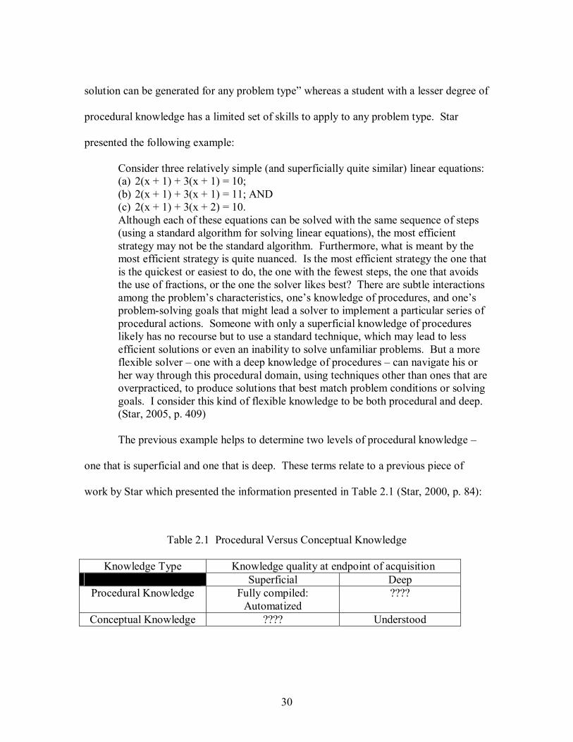
work by Star which presented the information presented in Table 2.1 (Star, 2000, p. 84):

Table 2.1 Procedural Versus Conceptual Knowledge

Knowledge Type Knowledge quality at endpoint of acquisition Superficial Deep

Procedural Knowledge Fully compiled: Automatized

????

Conceptual Knowledge ???? Understood

31

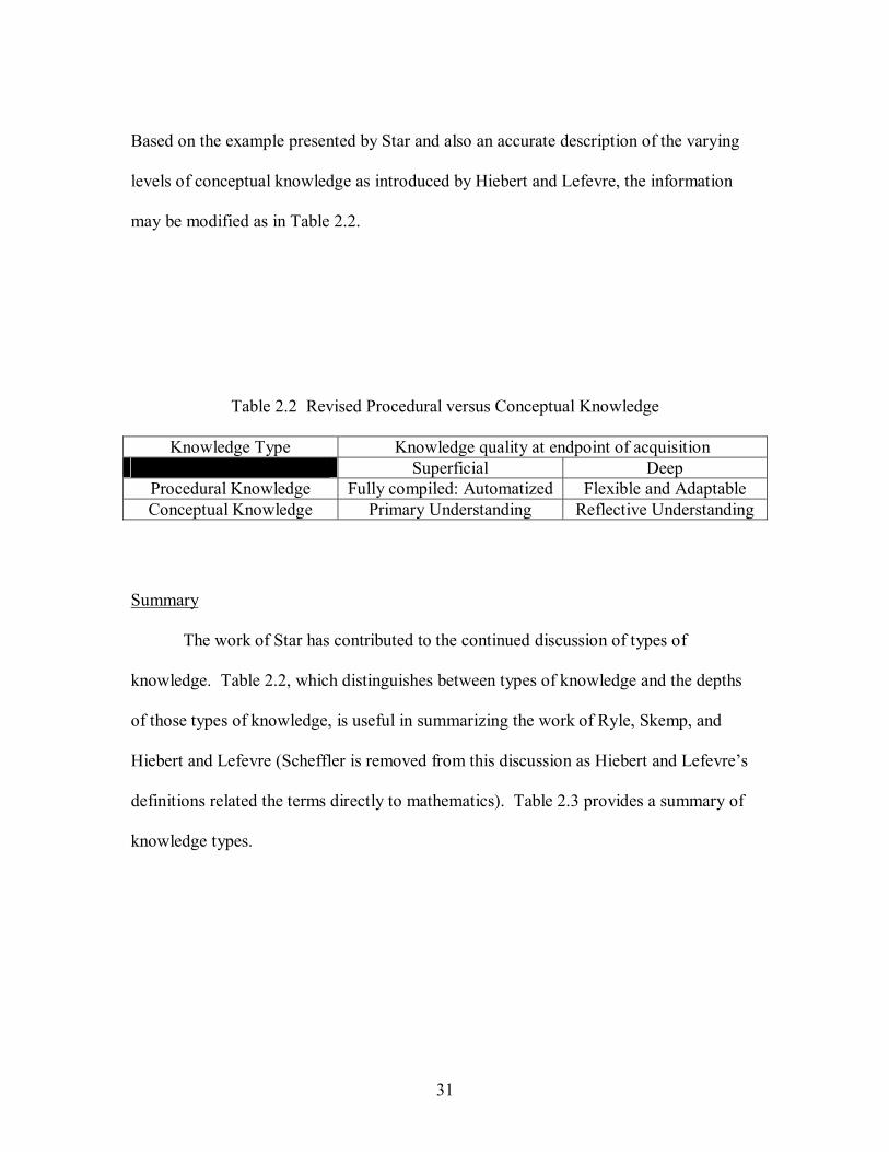
Based on the example presented by Star and also an accurate description of the varying

levels of conceptual knowledge as introduced by Hiebert and Lefevre, the information

may be modified as in Table 2.2.

Table 2.2 Revised Procedural versus Conceptual Knowledge

Knowledge Type Knowledge quality at endpoint of acquisition Superficial Deep

Procedural Knowledge Fully compiled: Automatized Flexible and Adaptable Conceptual Knowledge Primary Understanding Reflective Understanding

Summary

The work of Star has contributed to the continued discussion of types of

knowledge. Table 2.2, which distinguishes between types of knowledge and the depths

of those types of knowledge, is useful in summarizing the work of Ryle, Skemp, and

Hiebert and Lefevre (Scheffler is removed from this discussion as Hiebert and Lefevre�s

definitions related the terms directly to mathematics). Table 2.3 provides a summary of

knowledge types.

32

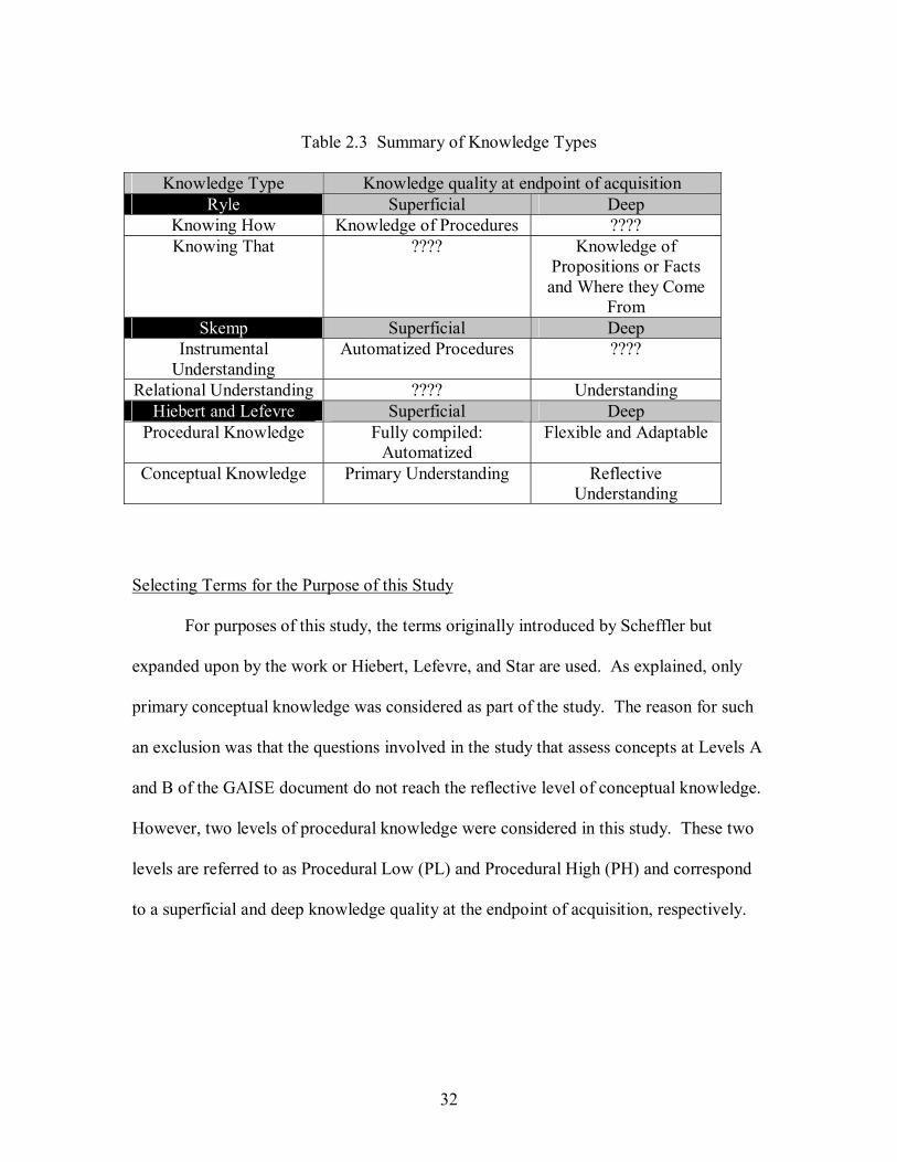
Table 2.3 Summary of Knowledge Types

Knowledge Type Knowledge quality at endpoint of acquisition Ryle Superficial Deep

Knowing How Knowledge of Procedures ???? Knowing That ???? Knowledge of

Propositions or Facts and Where they Come

From Skemp Superficial Deep

Instrumental Understanding

Automatized Procedures ????

Relational Understanding ???? Understanding Hiebert and Lefevre Superficial Deep

Procedural Knowledge Fully compiled: Automatized

Flexible and Adaptable

Conceptual Knowledge Primary Understanding Reflective Understanding

Selecting Terms for the Purpose of this Study

For purposes of this study, the terms originally introduced by Scheffler but

expanded upon by the work or Hiebert, Lefevre, and Star are used. As explained, only

primary conceptual knowledge was considered as part of the study. The reason for such

an exclusion was that the questions involved in the study that assess concepts at Levels A

and B of the GAISE document do not reach the reflective level of conceptual knowledge.

However, two levels of procedural knowledge were considered in this study. These two

levels are referred to as Procedural Low (PL) and Procedural High (PH) and correspond

to a superficial and deep knowledge quality at the endpoint of acquisition, respectively.

33

Conclusion

The terms identified are used to facilitate the discussion of what elementary

school teachers �understand� in relation to essential topics introduced in the GAISE

document at Levels A and B. The method by which the understanding of elementary

school teachers was examined is presented in the next chapter.

34

CHAPTER THREE

METHOD

This chapter presents the methods that were used to answer the following

questions:

1. What is the understanding of elementary school teachers in the following areas of

statistics: data displays, measures of central tendency, and measures of variation?

2. Does the implementation of the curricula materials and exposure to advanced

assessment instruments influence elementary school teachers� awareness of their

understanding of statistics?

This chapter is divided into six sections. The first section describes the setting of the

study. The second section describes the rationale for a qualitative design, the type of

design used, the role of the researcher, the selection of the participants, and the

participants. The third section provides a discussion of the Math Out of the Box materials

and how the topics covered compare to the GAISE document in relation to data displays,

measures of central tendency, and measures of variation. The fourth section describes the

phases of data collection. The fifth section discusses the methods of verification used in

this study. The concluding section contains a discussion of the limitations of the study.

Setting

This study was conducted in a middle- to upper-middle class school district

located in central New Jersey. Demographic data for the district are provided from the

New Jersey School Report Cards for each of the seven schools in the district. Two of the

35

seven schools were involved in this study. This information was provided by the New

Jersey Department of Education.

In the 2005-06 academic year, a total of 4,221 students attended the seven schools

in the district. Of the two schools involved in this study, one served students in grades K-

3 (School X) and the other served students in grades 4-6 (School Y). School X had a

total of 220 students with 53 in kindergarten, 53 in first-grade, 44 in second-grade, 46 in

third-grade, and 24 in special education programs. School X had a total of 20 teachers to

serve the 220 students creating a student to teacher ratio of 11 to 1. School Y had a total

of 898 students with 249 in fourth-grade, 266 in fifth-grade, 248 in sixth-grade, and 135

in special education programs. There were a total of 75 teachers at School Y creating a

student to teacher ratio of approximately 12 to 1.

In the state of New Jersey, an annual assessment is given entitled the NJASK. In

2005-06 the percent of third- and fourth-grade students at schools X and Y that were

judged to be either proficient or advanced on the mathematics assessment were 84.7%

and 76.6%, respectively. Third- and fourth-graders throughout the state were 82.4% and

82.3% proficient or advanced, respectively. Scores are reported for third- and fourth-

grade students since those are the grade levels taught by the three participants.

Qualitative Design, Role of Researcher, and Participants

Assumption and Rationale for a Qualitative Design

The questions of interest required analysis of three particular elementary school

teachers� understanding of various statistical topics. �Understanding of statistical topics�

36

cannot be easily identified or described. A qualitative design shed light on the status of

elementary school teachers� understanding of various statistical topics and how their

awareness of their understanding changed. Classroom observations provided a vehicle to

develop a clearer picture of elementary school teachers� understanding of various

statistical topics. The researcher spent more than 100 hours over the course of 14 months

in the field conducting observations and interviews.

The Type of Design Used

A qualitative approach was appropriate for this study because it offered methods

that were more suitable for collecting evidence to answer the research questions. There

was ample time for the collection of data from a number of sources. A case study was

used to describe the influences of implementing Math Out of the Box. The �case� for this

study was three particular elementary school teachers as they implemented this new

curriculum with ten lessons focused on data analysis and statistics. The case was a

�bounded system,� bounded by the amount of time it took the teachers to introduce the

concepts contained in the ten lessons during the spring and fall of 2006. There were

extensive, multiple sources of information. The data collected was triangulated to help

�tell the story� of these particular teachers.

The Role of the Researcher

The researcher served as a passive observer during classroom visits and as an

active participant in interviews with the teachers. Because of the rapport developed by

the researcher with the participants, open lines of communication were established. The

37

participants opened their classrooms and readily discussed their practices and

understanding of statistical ideas with the researcher.

Selection of Participants

Initial contact was made with the three teachers through a gatekeeper, the district

supervisor for mathematics and science education. She recommended a group of teachers

to participate in the study based on their qualifications and high standing in the district.

Several teachers were observed, interviewed, and surveyed before deciding on three

teachers as the focus of this case study. The study was limited to three participants

because of convenience sampling and the length of time necessary to visit, interview, and

assess the teachers at the depth involved in this study. The three participants were

selected because they were more willing to dedicate the necessary time involved with the

study than the other teachers and were open regarding their understanding of statistics.

Despite a self-reported dislike for the discipline of mathematics (discussion

forthcoming), the participants enjoyed teaching mathematics and looked forward to the

opportunity of teaching the statistical lessons contained in the Math Out of the Box

materials. All three teachers were highly recommended for this study as they were

viewed as exemplary teachers of mathematics by their principals and district supervisor.

The teachers were open regarding their misconceptions concerning the material. This

openness helped inform the researcher on the status of elementary school teachers�

understanding of various statistical topics.

38

Participants

This study involved two third-grade teachers, Ms. Brown and Ms. Clark, and one

fourth-grade teacher, Ms. Alvin (all pseudonyms). Ms. Brown and Ms. Clark were

teachers at School X and Ms. Alvin was a teacher at School Y. Ms. Alvin was the most

senior of the three with 9 years experience. Ms. Brown and Ms. Clark had 5 and 4 years

experience, respectively. Ms. Alvin was the only teacher with a Master�s degree (in

general education).

Ms. Alvin. Ms. Alvin had taught all nine years at the fourth-grade level. She

readily admitted mathematics was not her strong point. In college, she intentionally

avoided a mathematics course for as long as possible. In fact, she was able to take

physics to fulfill the mathematics requirement. Consequently, Ms. Alvin did not take any

undergraduate courses for teaching mathematics specifically at the elementary school

level, and only a single graduate mathematics teaching course.

Aside from the professional development (discussion forthcoming) related to the

implementation of Math Out of the Box, Ms. Alvin had not participated in any hours of

professional development related to mathematics education in the past six months. In the

past three years, she had participated in fewer than six hours of professional development

related to mathematics education. These values were self-reported and a description of

these professional development experiences was not available at the time of this study.

Ms. Alvin was a member of the National Educational Association and the New

Jersey Educational Association. She was not a member of any professional organizations

related to the teaching of mathematics. She was familiar with the New Jersey Core

39

Curriculum Content Standards, but, before the baseline interview (discussion

forthcoming) was unaware of the NCTM Standards, even though the New Jersey Core

Curriculum Content Standards were based on them.

Ms. Brown. Ms. Brown had taught all five years at the third-grade level. Like

Ms. Alvin, she readily admitted to not being particularly good at mathematics. Ms.

Brown took a college algebra course as a freshman to satisfy the mathematics

requirement as soon as possible. She also took a course in mathematics for elementary

school teachers in her junior year.

Aside from the professional development related to the implementation of Math

Out of the Box, Ms. Brown had participated in fewer than six hours of professional

development related to mathematics education in the past six months. In the past three

years, she had participated in 16-35 hours related to mathematics education. These

values were self-reported and a description of these professional development

experiences was not available at the time of this study.

Ms. Brown was not a member of any professional organizations. She

remembered hearing about the NCTM Standards when she was in college, but did not

remember them well. However, she was familiar with the New Jersey Core Curriculum

Content Standards.

Ms. Clark. Ms. Clark had taught all four years at the third-grade level. She too

readily admitted to an aversion to mathematics. In college she took an algebra class that

she remembered quite well due to her struggles with the subject. She took this course as

40

a senior after putting off the mathematics requirement for as long as possible. Like Ms.

Brown, she too took a course in mathematics for elementary school teachers in her junior

year.

Aside from the professional development related to the implementation of Math

Out of the Box, Ms. Alvin had participated in fewer than 6 hours of professional

development related to mathematics education in the past six months. In the past three

years, she had participated in between 6-15 hours of professional development. These

values were self-reported and a description of these professional development

experiences was not available at the time of this study.

Ms. Clark was a member of the National Educational Association and the New

Jersey Educational Association. Like the other two teachers, she was familiar with the

New Jersey Core Curriculum Content Standards but unfamiliar with the NCTM

Standards.

Math Out of the Box Materials

The following description of the materials was verified by an independent

reviewer who is an expert in curriculum and assessment. The curriculum materials

serving as the medium in this study build the content around real data collection

activities. The activities address many of the objectives identified at Level A in the

GAISE. Specifically, in grades 3 and 4 the first four objectives at Level A are touched

upon. The content at grades 3 and 4 is similar and the tasks guide students in formulating

questions, understanding that data are more than just numbers, and using tools (including

data displays, measures of central tendency, and measures of variation) to analyze data.

41

Data Displays

Similar data displays are utilized in grades 3 and 4. The students learn to

construct and interpret tally and frequency tables, line plots (similar to dotplots with X�s

instead of dots), and line graphs (time plots). The teacher manual in grades 3 and 4

encourages the teachers to ask students to represent data in multiple ways (e.g. tally

tables and line plots) so that they may be able to realize the advantages and disadvantages

of each display. However, those advantages or disadvantages are not discussed in the

materials themselves.

Measures of Central Tendency

The mode and median are the only measures of central tendency introduced in

grades 3 and 4. The mode is defined as the value that occurs most often. It is mentioned

on multiple occasions that a data set can have one mode, more than one mode, or no

mode. However, an example is not provided where a data set has more than one mode or

no mode. The median is defined as the middle value. The materials discuss finding a

median in a data set with an odd and even number of values. The mode is described as

the only acceptable measure of central tendency for a categorical variable. However, the

advantages and disadvantages of each measure of central tendency are not discussed.

Measures of Variation

The range is the only measure of variation introduced in grades 3 and 4. The

range is defined as the difference between the highest and lowest values. The materials

do not specifically indicate that the range is an inappropriate measure of variation for

42

categorical variables. The teacher manual indicates that the range provides information

about the spread of the data. It also indicates that a larger range generally implies the

data are more spread out.

Outliers (a topic related to measures of variation) are also introduced in grades 3

and 4. The teacher manual defines an outlier as �a value that falls far removed from

others in a data set.� The calculations for finding such a value are not discussed at either

grade level. The manual also indicates that often �an outlier is the result of a mistake in

the data collection process�in statistical analysis, an outlier is discarded when a whole

data set is examined� (Moss et al. 2005a, Grade 3, p. 157).

Summary

The data lessons in the Math Out of the Box materials involve some topics at the

level of sophistication described in the GAISE. The fact that the materials build the

content around real data encourages students to grasp the true essence of statistics.

However, the materials do not discuss the advantages and disadvantages of various data

displays, measures of central tendency, or measures of variation. These topics are

discussed during professional development provided by the creators of the curriculum

(discussion forthcoming). This study sheds light on whether or not elementary school

teachers possess sufficient understanding of the statistical topics described above. The

Math Out of the Box materials served as a powerful medium for such an exploration.

43

Three Phases of Data Collection

There were three phases of data collection. In Phase One, during the fall of 2005,

baseline data were collected on the teachers. In Phase Two, during the spring of 2006,

data were collected on the teachers as they implemented the Math Out of the Box

materials. In the case of Ms. Alvin, the implementation of the materials was for the

second time. However, during her first implementation she did not have time to complete

all of the lessons of the unit. The study had not begun prior to her implementation of the

materials for the first time. For Ms. Brown and Ms. Clark the spring of 2006 represented

their first use of the materials. In Phase Three, during the fall of 2006, data were

collected as the teachers implemented the materials for the second or third time. A table

summarizing the instruments used during each phase of data collection is provided at the

end of this section.

Phase One

Baseline data were collected during Phase One. This phase involved meeting

with the teachers and conducting a baseline interview before the first, or in the case of

Ms. Alvin second, implementation of the Math Out of the Box materials.

The baseline interview provided baseline data regarding the teachers� educational

background, experience, level of participation in professional development, and comfort

level with teaching data analysis and statistics. (Results were used in the above

discussion of the participants.) The 45-minute interview was conducted prior to use of

Math Out of the Box for Ms. Brown and Ms. Clark and after one implementation for Ms.

44

Alvin. One-on-one interviews were conducted with each teacher involved in the study.

See Appendix A for a copy of this interview.

Phase Two

Phase Two began with the professional development training focused on statistics

which was offered by the creators of the Math Out of the Box materials. The key

component of data collection during this phase involved observations of the teachers as

they implemented the statistical lessons of the Math Out of the Box Materials. There

were also two formal interviews conducted after the implementation of the materials.

Researcher Presence During Professional Development Activities. The researcher

was present during one eight-hour professional development training which focused on

statistical topics. The training was provided by the developers of Math Out of the Box

materials. During this one eight-hour session, the researcher sat with the teachers and

took notes. The following description of the professional development activities was

provided by the main professional development facilitator (Diaz, E-mail Correspondence,

4/16/2007). All of the teachers participated in sample activities for the K-5 curriculum

regardless of which grade they were teaching.

Description of Professional Development Activities. The professional

development is a K-5 overview of topics that provides teachers with a "big picture" of

how some of the topics in data analysis are developed through the Math Out of the Box

materials.

45

K-1 Focus. The day begins with a sorting activity and teachers sort the same

collection a couple of different ways. In the first sorting activity one group of teachers

sort a collection of objects and another group of teachers have to try to figure out the sort.

In the second sorting activity, they have to sort using a new rule and to create a display

that communicates the rule of sort they used. Teachers begin to learn that the purpose of

displaying data is to share information and discussions are facilitated to help teachers

understand how conventions used in data displays help communicate the information

about the data.

2-3 Focus. The second part of the data professional development focuses on the

importance of a "fair test." Teachers collect data about their wrist sizes. This is an actual

lesson in the grade 3 materials and the session models for the teachers some of the issues

that will arise in their own classrooms. Teachers are asked to provide some questions

about their wrists. After these questions are charted, a discussion is facilitated about how

the question determines the type of data that is collected. Teachers collect data about

their wrists (e.g. the circumference, width on top, width on bottom) and the importance of

describing specific details about data collection is discussed based on the outcomes of the

varied data that are collected without any specific directions. Various means of

organizing the data are discussed, particularly tabular methods. The group eventually

decides on collecting data regarding each participant�s wrist circumference and a line plot

is constructed to display these measurements.

46

4-5 Focus. The line plot from the wrist data is used to discuss statistical

information including the range, mode, and median. An investigation is carried out by

the group about counting the number of steps over a certain distance. Teachers set up

specifications for data collection, collect and organize the data and display their results.

Statistical information about the data is figured and discussed within the context of the

data set. The meaning of the mode, range, and median for that particular sample is

discussed, so that the definitions (which teachers tend to know "by heart") are given

meaning in the context of something they have experienced. Mode is not just the "most"

but it is the number of steps taken over a certain length by the most number of teachers in

the group. The range is not just the "most minus least" but the difference between the

most steps taken and the least steps taken, so one can know if there is really a big range

of difference in the group. The median is not just "the middle" but it means that the same

number of people in the group walked fewer steps than the median as walked more steps

than the median.

General. Teachers also do a leveling activity to examine the mean. The mean

is included in the professional development materials so teachers may begin to

understand the differences between the various measures of center. As discussed

previously, the only measures of center in the student materials are the median and the

mode. In this activity, the mean, median, and mode for teachers� shoe sizes is found and

their meanings and differences are discussed in the context of the data set. (Note: If there

are males present in the group, participants decide how to deal with that issue in regard to

appropriate methods of data collection.)

47

Observations. The researcher served as a passive observer during five classroom

visits per teacher. Transcripts of the lessons were composed. These transcripts were

used to analyze the statistical content covered in each class as well as to determine if any

misconceptions were exhibited by the teachers during instruction or in responses to

student questions. Appendix B is an example of the observational protocol.

Statistical Content Interview. This 30-minute interview asked teachers to define

common statistical terms that appear in the Math Out of the Box materials, discuss how

these measurements can be calculated, and why they may be useful. In relation to these

topics, teachers were asked to indicate whether or not their level of understanding of

these topics changed as a result of the use of the materials. This interview assessed the

teachers� possible change in understanding during Phase Three of data collection.

Appendix C is the form used for this interview.

Math Out of the Box Interview. This 45-minute interview provided feedback

during implementation of the Math Out of the Box curriculum. The questions contained

in this interview assessed teacher learning after the implementation of the Math Out of

the Box materials. The questions in this interview were based on the work of Diaz

(2004). Appendix D is the form used for this interview.

Phase Three

Phase Three served as the major component of data collection. This phase

represented a time when all the teachers had already implemented the statistical lessons at

least one time. During Phase Three, Observations, the Statistical Content Interview, and

48

the Math Out of the Box Interview were used as described in Phase Two. In addition, the

teachers� content knowledge was assessed as described below..

Assessments. In addition to the repeated administration of the Statistical Content

Interview, a more in-depth analysis of teachers� understanding of statistics was conducted

during Phase Three. This level of analysis involved topics related to the concepts

introduced at their particular grade level. However, the content of these assessments also

involved a more sophisticated level of understanding of statistics as proposed by the

GAISE. In particular these questions involved material related to data displays, measures

of central tendency, and measures of variation. Questions were taken from established

assessments such as the NAEP and Diagnostic Teacher Assessments in Mathematics and

Science developed at the University of Louisville. These assessments have established

high levels of reliability and validity (Bush, et al, under review). These assessments also

contained questions developed by the researcher who was a mathematics assessment

specialist. One of these questions was related to a question posed on the 2006 AP®

Statistics exam. This particular question was chosen because it pulled together how

measures of central tendency and variation can be used to make a decision and was

judged to be accessible by elementary school teachers. The decision to include this

particular question, based on the entry level available to elementary school teachers, was

confirmed by an independent reviewer who was also an assessment specialist in

mathematics. Appendices E, F, G, H, and I contain the questions used in these

assessments.

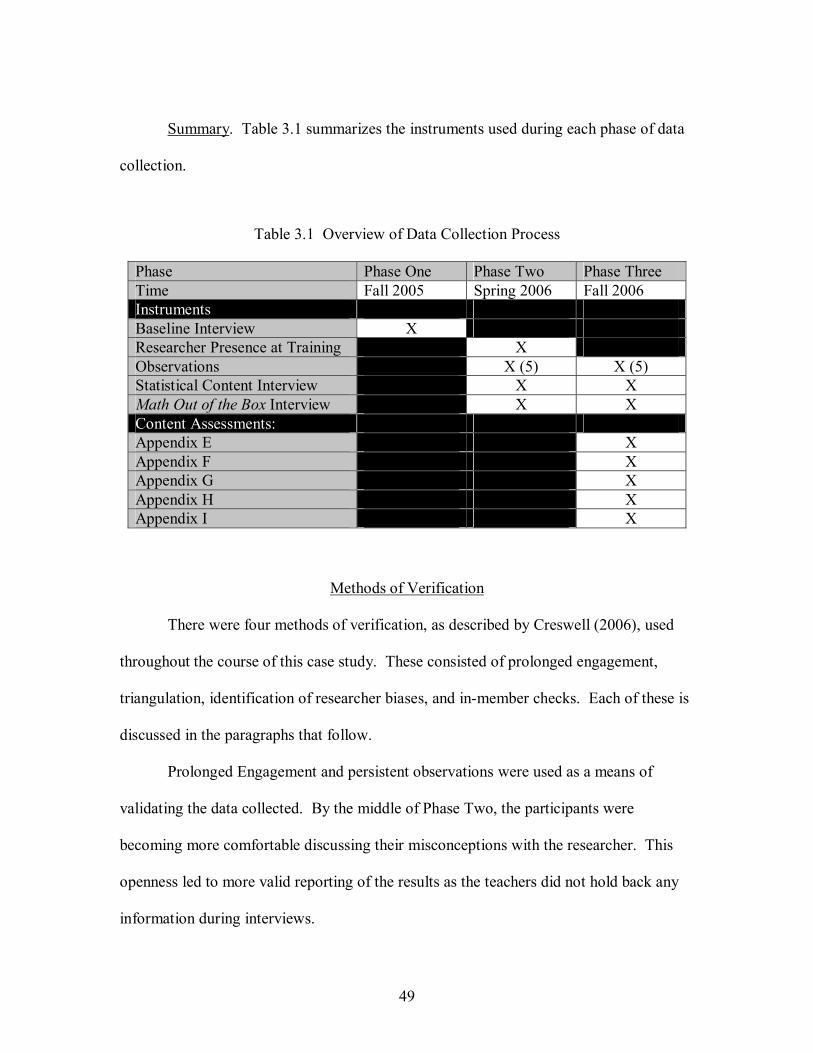
49

Summary. Table 3.1 summarizes the instruments used during each phase of data

collection.

Table 3.1 Overview of Data Collection Process

Phase Phase One Phase Two Phase Three Time Fall 2005 Spring 2006 Fall 2006 Instruments Baseline Interview X Researcher Presence at Training X Observations X (5) X (5) Statistical Content Interview X X Math Out of the Box Interview X X Content Assessments: Appendix E X Appendix F X Appendix G X Appendix H X Appendix I X

Methods of Verification

There were four methods of verification, as described by Creswell (2006), used

throughout the course of this case study. These consisted of prolonged engagement,

triangulation, identification of researcher biases, and in-member checks. Each of these is

discussed in the paragraphs that follow.

Prolonged Engagement and persistent observations were used as a means of

validating the data collected. By the middle of Phase Two, the participants were

becoming more comfortable discussing their misconceptions with the researcher. This

openness led to more valid reporting of the results as the teachers did not hold back any

information during interviews.

50

Triangulation was one of the primary sources for validation in this case study.

Nine different instruments were used during data collection. Each instrument involved in

the study was analyzed separately and then compared with other instruments to verify the

data provided an accurate view of the teachers� understanding. The process involved

corroborating evidence from the multiple sources in order to provide insight into the

status of elementary school teachers� statistical understanding.

Researcher biases are clarified later in this chapter. The audience must

understand the position of the researcher. The influences of past experiences that may

have biased the researcher are discussed in order to ensure an accurate interpretation can

be taken.

In-member checks were another major source of reliability. Lincoln and Guba

(1985) state that in-member checks are �the most critical technique of establishing

credibility� (p. 314). At several points during the collection of data and especially at the

conclusion of the study, participants were asked to verify reports that resulted from their

participation. In particular, the participants were presented with transcripts of the

observations and interviews and asked to ensure that the transcriptions were accurate

descriptions of what had transpired. During these in-member checks, there was not a

single area of disagreement between the researcher and the participants. This method of

verification was crucial to establishing reliability in this study.

Limitations

There are many advantages to conducting a qualitative case study; however there

are also limitations. First of all, this study was limited by the sample size. By examining

51

only three teachers, generalizations to all elementary school teachers are not appropriate.

However, since these teachers were highly recommended by their district supervisor and

principals as exemplary teachers of mathematics, they provide a snapshot of what may be

expected of exemplary elementary school teachers� understanding of certain statistical

topics.

Secondly, this study was influenced by the biases of the researcher. The

researcher believed elementary school teachers should possess an in-depth understanding

of statistics (and mathematics). It is only with an in-depth understanding that teachers

can appropriately respond to students� questions and push their thinking in new

directions. The researcher also speculated that most elementary school teachers (and

teachers at all levels) do not possess the understanding the authors of the GAISE

document suggest. If teachers do not possess the understanding expected of students then

it is difficult to create learning environments where students� understanding can reach an

adequate level. The researcher believed that most teachers, especially elementary school

teachers, view mathematics in a negative fashion.

Inherently, these acknowledged biases may have had an impact on the analysis of

this study. These biases may have caused the researcher to examine teachers�

understanding from a deficit rather than constructivist view. In other words, the study

focused more on the identification of misconceptions and shortcomings in the teachers�

understanding rather than viewing the understanding the teachers possessed as a building

block for future learning. These biases also influenced the selection of the research

questions. However, the realization of these biases caused the researcher to pay close

52

attention to the data collected and reduce the influence of these biases in assessing the

understanding of the teachers.

Conclusion

The Math Out of the Box materials served as a powerful medium to investigate

three elementary school teachers� understanding of essential statistical topics. Based on

the rationale for a qualitative design and the methods of verification, the results presented

in the following chapter are both reliable and valid.

53

CHAPTER FOUR

ANALYSIS AND RESULTS

This chapter presents the analysis and results of the study. The first section

categorizes the questions contained in each instrument based on the content (i.e. data

displays, measures of central tendency, and measures of variation) and the type of

knowledge assessed (i.e. procedural low, procedural high, and conceptual). The results

and data analysis are contained in the next five sections. The second section is an

analysis of the teachers� performance in the area of data displays, the third is an analysis

of the teachers� performance in the area of measures of central tendency, and the fourth is

an analysis of the teachers� performance in the area of measures of variation. The fifth

section makes connections between the teachers� understanding and the

recommendations contained in the GAISE document. The concluding section discusses

the teachers� awareness of their understanding.

Categorization of the Questions

This section organizes questions in the following categories: data displays,

measures of central tendency, and measures of variation. Tables 4.1, 4.2, and 4.3 show

the categorization of each question contained in the content knowledge instruments

(Appendices E, F, G, H, and I). Each question was identified as either multiple-choice

(MC) or open-ended (OE) and categorized as assessing procedural-low (PL), procedural-

high (PH), or conceptual knowledge (C). The categorizations indicated in the table have

been verified by two independent reviewers who are mathematics assessment specialists.

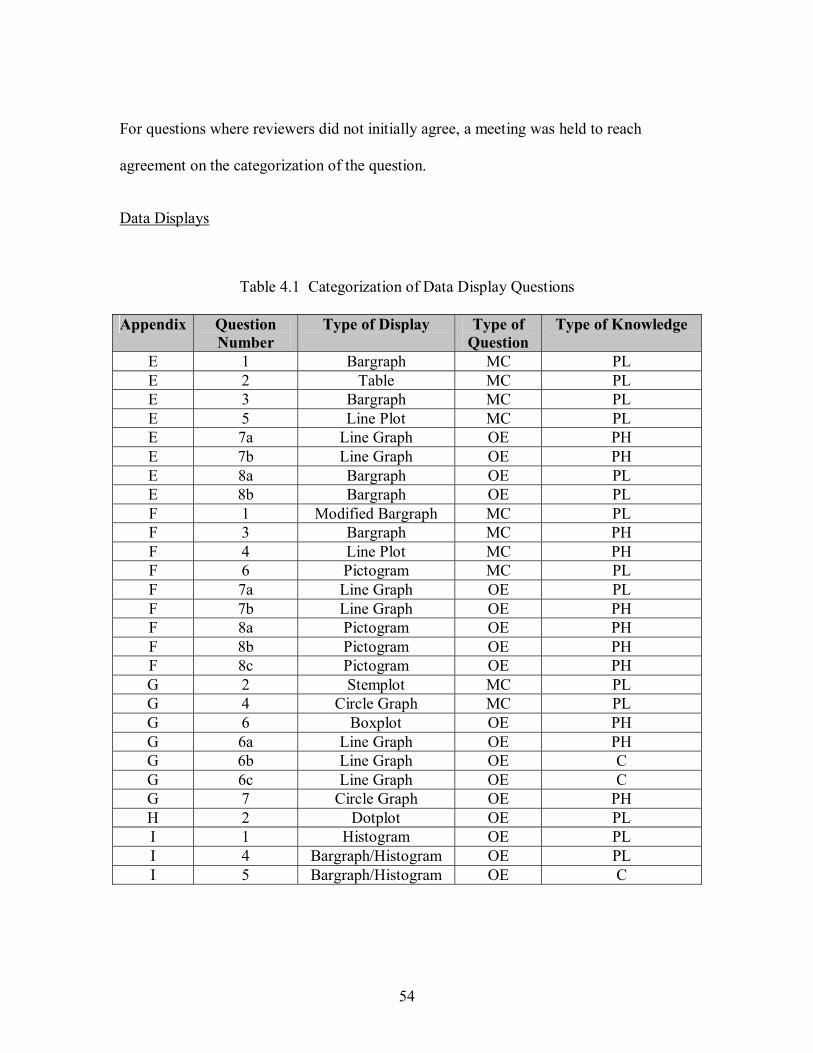
54

For questions where reviewers did not initially agree, a meeting was held to reach

agreement on the categorization of the question.

Data Displays

Table 4.1 Categorization of Data Display Questions

Appendix Question Number

Type of Display Type of Question

Type of Knowledge

E 1 Bargraph MC PL E 2 Table MC PL E 3 Bargraph MC PL E 5 Line Plot MC PL E 7a Line Graph OE PH E 7b Line Graph OE PH E 8a Bargraph OE PL E 8b Bargraph OE PL F 1 Modified Bargraph MC PL F 3 Bargraph MC PH F 4 Line Plot MC PH F 6 Pictogram MC PL F 7a Line Graph OE PL F 7b Line Graph OE PH F 8a Pictogram OE PH F 8b Pictogram OE PH F 8c Pictogram OE PH G 2 Stemplot MC PL G 4 Circle Graph MC PL G 6 Boxplot OE PH G 6a Line Graph OE PH G 6b Line Graph OE C G 6c Line Graph OE C G 7 Circle Graph OE PH H 2 Dotplot OE PL I 1 Histogram OE PL I 4 Bargraph/Histogram OE PL I 5 Bargraph/Histogram OE C

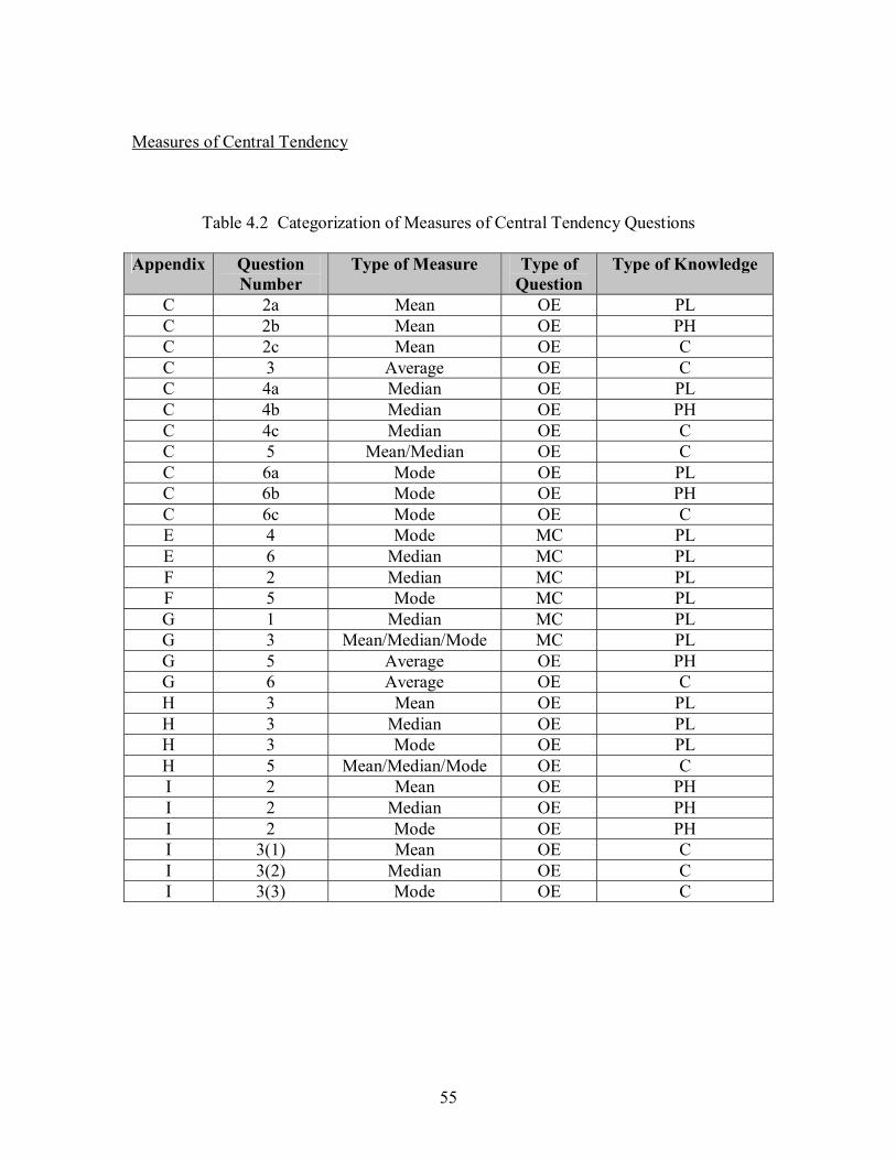
55

Measures of Central Tendency

Table 4.2 Categorization of Measures of Central Tendency Questions

Appendix Question Number

Type of Measure Type of Question

Type of Knowledge

C 2a Mean OE PL C 2b Mean OE PH C 2c Mean OE C C 3 Average OE C C 4a Median OE PL C 4b Median OE PH C 4c Median OE C C 5 Mean/Median OE C C 6a Mode OE PL C 6b Mode OE PH C 6c Mode OE C E 4 Mode MC PL E 6 Median MC PL F 2 Median MC PL F 5 Mode MC PL G 1 Median MC PL G 3 Mean/Median/Mode MC PL G 5 Average OE PH G 6 Average OE C H 3 Mean OE PL H 3 Median OE PL H 3 Mode OE PL H 5 Mean/Median/Mode OE C I 2 Mean OE PH I 2 Median OE PH I 2 Mode OE PH I 3(1) Mean OE C I 3(2) Median OE C I 3(3) Mode OE C

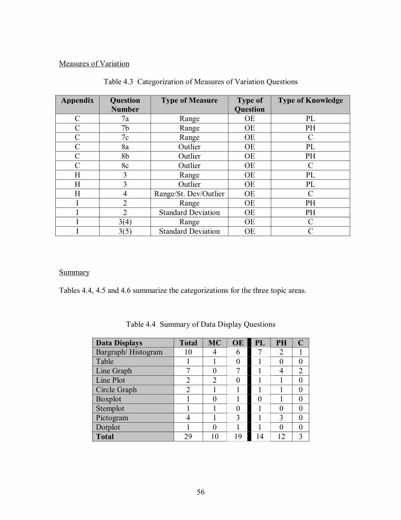
56

Measures of Variation

Table 4.3 Categorization of Measures of Variation Questions

Appendix Question Number

Type of Measure Type of Question

Type of Knowledge

C 7a Range OE PL C 7b Range OE PH C 7c Range OE C C 8a Outlier OE PL C 8b Outlier OE PH C 8c Outlier OE C H 3 Range OE PL H 3 Outlier OE PL H 4 Range/St. Dev/Outlier OE C I 2 Range OE PH I 2 Standard Deviation OE PH I 3(4) Range OE C I 3(5) Standard Deviation OE C

Summary

Tables 4.4, 4.5 and 4.6 summarize the categorizations for the three topic areas.

Table 4.4 Summary of Data Display Questions

Data Displays Total MC OE PL PH C Bargraph/ Histogram 10 4 6 7 2 1 Table 1 1 0 1 0 0 Line Graph 7 0 7 1 4 2 Line Plot 2 2 0 1 1 0 Circle Graph 2 1 1 1 1 0 Boxplot 1 0 1 0 1 0 Stemplot 1 1 0 1 0 0 Pictogram 4 1 3 1 3 0 Dotplot 1 0 1 1 0 0 Total 29 10 19 14 12 3

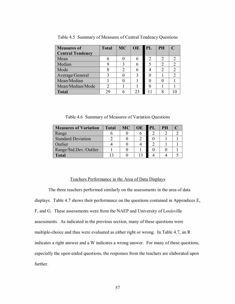
57

Table 4.5 Summary of Measures of Central Tendency Questions

Measures of Central Tendency

Total MC OE PL PH C

Mean 6 0 6 2 2 2 Median 9 3 6 5 2 2 Mode 8 2 6 4 2 2 Average/General 3 0 3 0 1 2 Mean/Median 1 0 1 0 0 1 Mean/Median/Mode 2 1 1 0 1 1 Total 29 6 23 11 8 10

Table 4.6 Summary of Measures of Variation Questions

Measures of Variation Total MC OE PL PH C Range 6 0 6 2 2 2 Standard Deviation 2 0 2 0 1 1 Outlier 4 0 4 2 1 1 Range/Std.Dev./Outlier 1 0 1 0 0 1 Total 13 0 13 4 4 5

Teachers Performance in the Area of Data Displays

The three teachers performed similarly on the assessments in the area of data

displays. Table 4.7 shows their performance on the questions contained in Appendices E,

F, and G. These assessments were from the NAEP and University of Louisville

assessments. As indicated in the previous section, many of these questions were

multiple-choice and thus were evaluated as either right or wrong. In Table 4.7, an R

indicates a right answer and a W indicates a wrong answer. For many of these questions,

especially the open-ended questions, the responses from the teachers are elaborated upon

further.

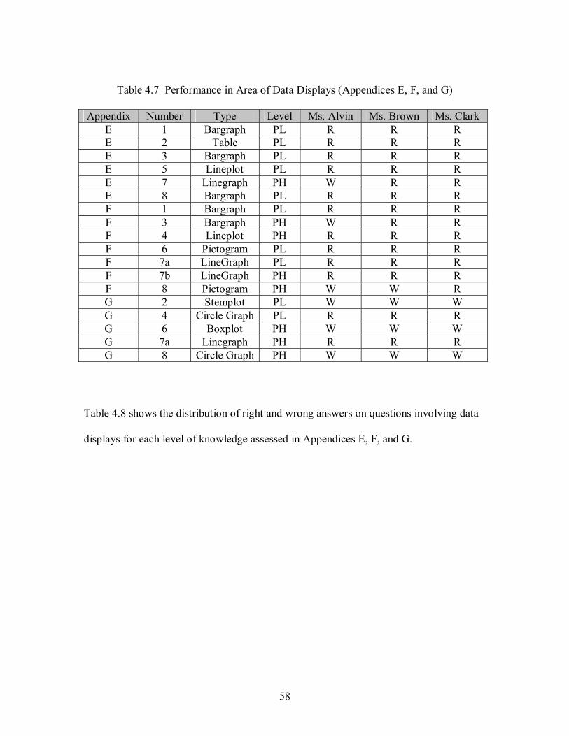
58

Table 4.7 Performance in Area of Data Displays (Appendices E, F, and G)

Appendix Number Type Level Ms. Alvin Ms. Brown Ms. Clark E 1 Bargraph PL R R R E 2 Table PL R R R E 3 Bargraph PL R R R E 5 Lineplot PL R R R E 7 Linegraph PH W R R E 8 Bargraph PL R R R F 1 Bargraph PL R R R F 3 Bargraph PH W R R F 4 Lineplot PH R R R F 6 Pictogram PL R R R F 7a LineGraph PL R R R F 7b LineGraph PH R R R F 8 Pictogram PH W W R G 2 Stemplot PL W W W G 4 Circle Graph PL R R R G 6 Boxplot PH W W W G 7a Linegraph PH R R R G 8 Circle Graph PH W W W

Table 4.8 shows the distribution of right and wrong answers on questions involving data

displays for each level of knowledge assessed in Appendices E, F, and G.

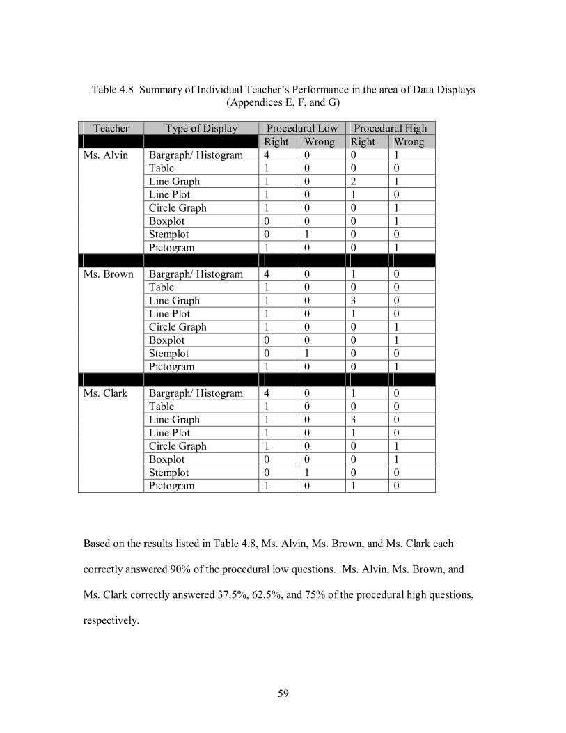
59

Table 4.8 Summary of Individual Teacher�s Performance in the area of Data Displays (Appendices E, F, and G)

Teacher Type of Display Procedural Low Procedural High

Right Wrong Right Wrong Bargraph/ Histogram 4 0 0 1 Table 1 0 0 0 Line Graph 1 0 2 1 Line Plot 1 0 1 0 Circle Graph 1 0 0 1 Boxplot 0 0 0 1 Stemplot 0 1 0 0

Ms. Alvin

Pictogram 1 0 0 1

Bargraph/ Histogram 4 0 1 0 Table 1 0 0 0 Line Graph 1 0 3 0 Line Plot 1 0 1 0 Circle Graph 1 0 0 1 Boxplot 0 0 0 1 Stemplot 0 1 0 0

Ms. Brown

Pictogram 1 0 0 1

Bargraph/ Histogram 4 0 1 0 Table 1 0 0 0 Line Graph 1 0 3 0 Line Plot 1 0 1 0 Circle Graph 1 0 0 1 Boxplot 0 0 0 1 Stemplot 0 1 0 0

Ms. Clark

Pictogram 1 0 1 0

Based on the results listed in Table 4.8, Ms. Alvin, Ms. Brown, and Ms. Clark each

correctly answered 90% of the procedural low questions. Ms. Alvin, Ms. Brown, and

Ms. Clark correctly answered 37.5%, 62.5%, and 75% of the procedural high questions,

respectively.

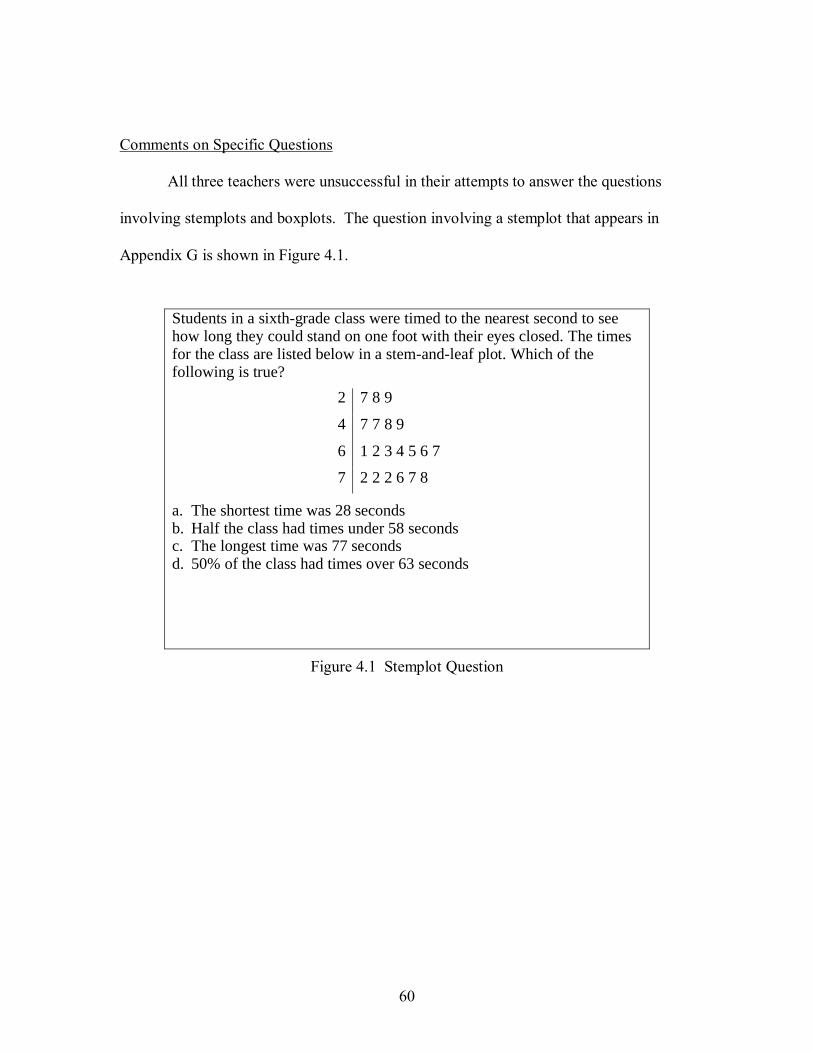
60

Comments on Specific Questions

All three teachers were unsuccessful in their attempts to answer the questions

involving stemplots and boxplots. The question involving a stemplot that appears in

Appendix G is shown in Figure 4.1.

Students in a sixth-grade class were timed to the nearest second to see how long they could stand on one foot with their eyes closed. The times for the class are listed below in a stem-and-leaf plot. Which of the following is true?

2 7 8 9

4 7 7 8 9

6 1 2 3 4 5 6 7

7 2 2 2 6 7 8

a. The shortest time was 28 seconds b. Half the class had times under 58 seconds c. The longest time was 77 seconds d. 50% of the class had times over 63 seconds

Figure 4.1 Stemplot Question

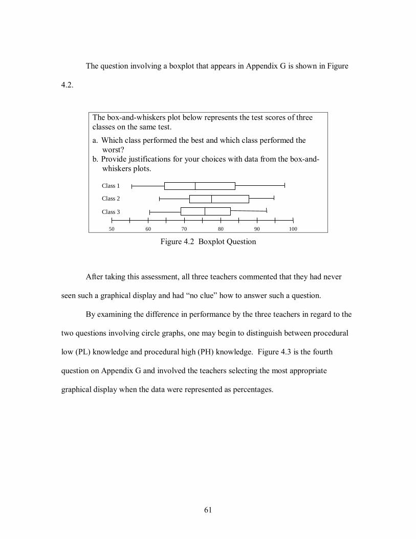
61

The question involving a boxplot that appears in Appendix G is shown in Figure

4.2.

The box-and-whiskers plot below represents the test scores of three classes on the same test. a. Which class performed the best and which class performed the

worst? b. Provide justifications for your choices with data from the box-and-

whiskers plots.

Figure 4.2 Boxplot Question

After taking this assessment, all three teachers commented that they had never

seen such a graphical display and had �no clue� how to answer such a question.

By examining the difference in performance by the three teachers in regard to the

two questions involving circle graphs, one may begin to distinguish between procedural

low (PL) knowledge and procedural high (PH) knowledge. Figure 4.3 is the fourth

question on Appendix G and involved the teachers selecting the most appropriate

graphical display when the data were represented as percentages.

50

Class 1 Class 2 Class 3

60 70 80 90 100

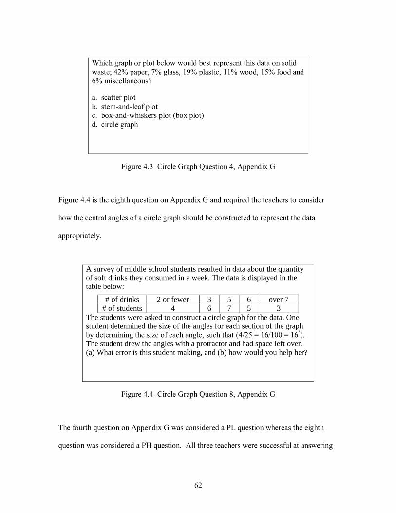
62

Which graph or plot below would best represent this data on solid waste; 42% paper, 7% glass, 19% plastic, 11% wood, 15% food and 6% miscellaneous?

a. scatter plot b. stem-and-leaf plot c. box-and-whiskers plot (box plot) d. circle graph

Figure 4.3 Circle Graph Question 4, Appendix G

Figure 4.4 is the eighth question on Appendix G and required the teachers to consider

how the central angles of a circle graph should be constructed to represent the data

appropriately.

A survey of middle school students resulted in data about the quantity of soft drinks they consumed in a week. The data is displayed in the table below:

# of drinks 2 or fewer 3 5 6 over 7 # of students 4 6 7 5 3

The students were asked to construct a circle graph for the data. One student determined the size of the angles for each section of the graph by determining the size of each angle, such that (4/25 = 16/100 = 16°). The student drew the angles with a protractor and had space left over. (a) What error is this student making, and (b) how would you help her?

Figure 4.4 Circle Graph Question 8, Appendix G

The fourth question on Appendix G was considered a PL question whereas the eighth

question was considered a PH question. All three teachers were successful at answering

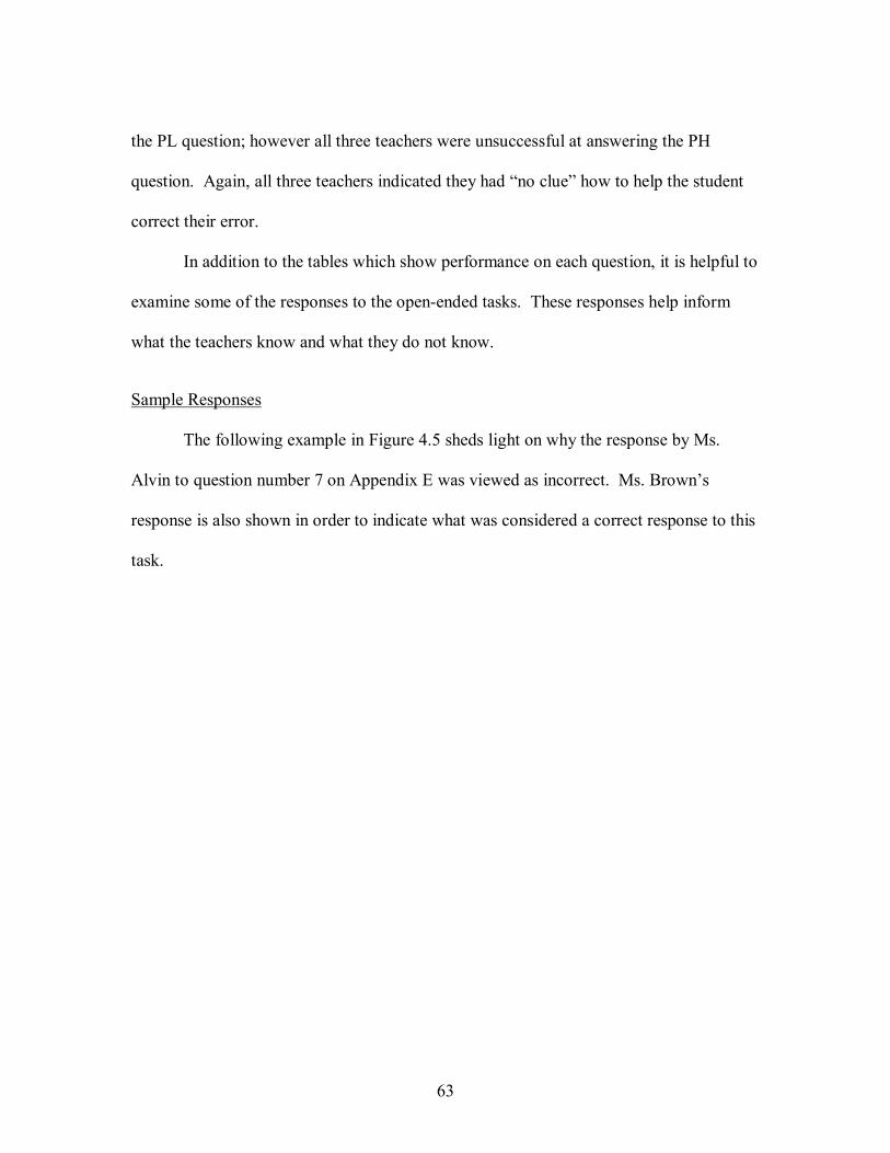
63

the PL question; however all three teachers were unsuccessful at answering the PH

question. Again, all three teachers indicated they had �no clue� how to help the student

correct their error.

In addition to the tables which show performance on each question, it is helpful to

examine some of the responses to the open-ended tasks. These responses help inform

what the teachers know and what they do not know.

Sample Responses

The following example in Figure 4.5 sheds light on why the response by Ms.

Alvin to question number 7 on Appendix E was viewed as incorrect. Ms. Brown�s

response is also shown in order to indicate what was considered a correct response to this

task.

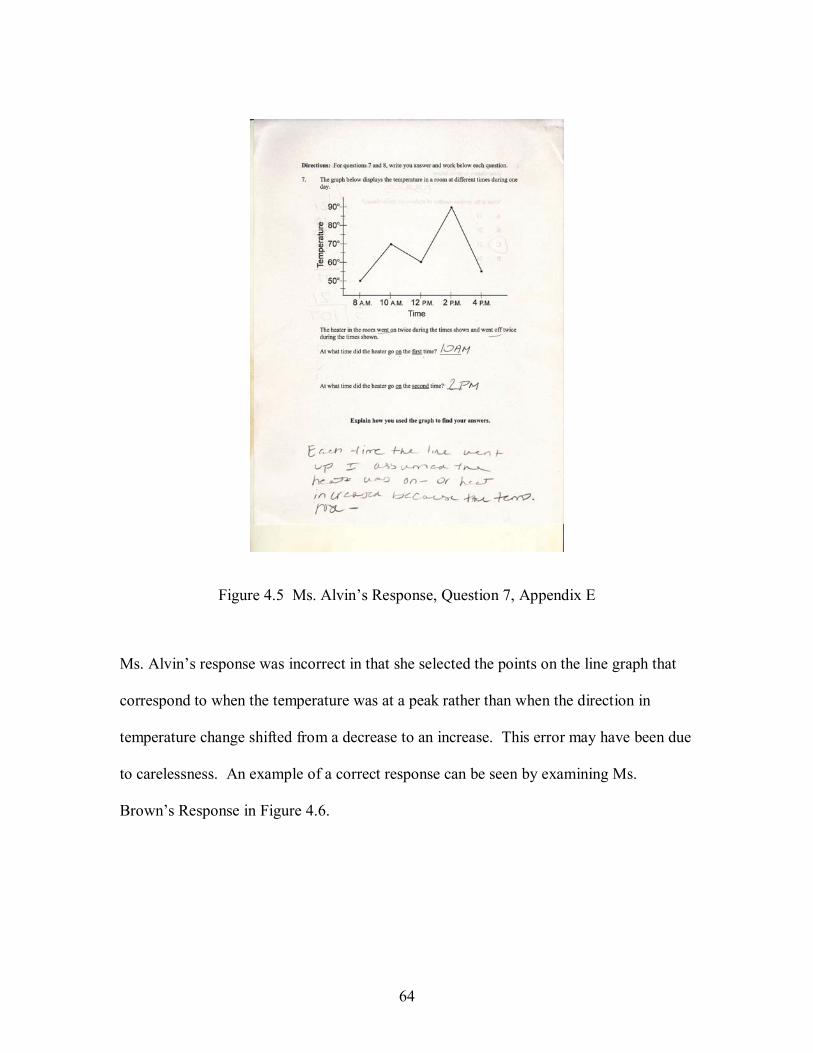
64

Figure 4.5 Ms. Alvin�s Response, Question 7, Appendix E

Ms. Alvin�s response was incorrect in that she selected the points on the line graph that

correspond to when the temperature was at a peak rather than when the direction in

temperature change shifted from a decrease to an increase. This error may have been due

to carelessness. An example of a correct response can be seen by examining Ms.

Brown�s Response in Figure 4.6.

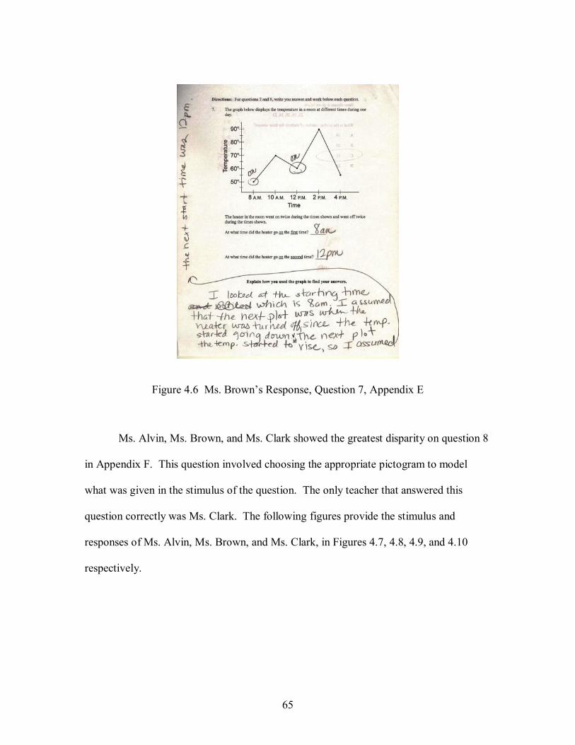
65

Figure 4.6 Ms. Brown�s Response, Question 7, Appendix E

Ms. Alvin, Ms. Brown, and Ms. Clark showed the greatest disparity on question 8

in Appendix F. This question involved choosing the appropriate pictogram to model

what was given in the stimulus of the question. The only teacher that answered this

question correctly was Ms. Clark. The following figures provide the stimulus and

responses of Ms. Alvin, Ms. Brown, and Ms. Clark, in Figures 4.7, 4.8, 4.9, and 4.10

respectively.

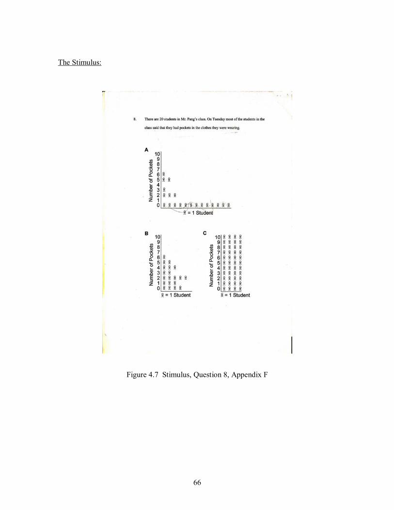
66

The Stimulus:

Figure 4.7 Stimulus, Question 8, Appendix F

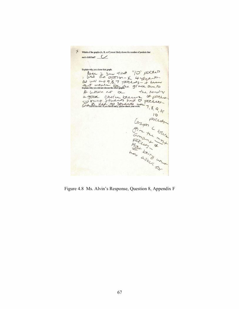
67

Figure 4.8 Ms. Alvin�s Response, Question 8, Appendix F

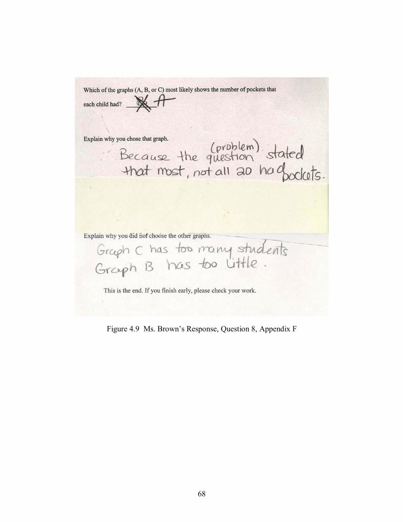
68

Figure 4.9 Ms. Brown�s Response, Question 8, Appendix F

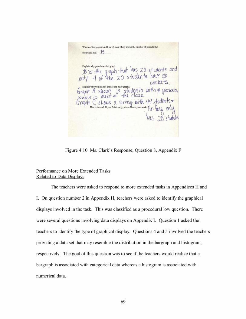
69

Figure 4.10 Ms. Clark�s Response, Question 8, Appendix F

Performance on More Extended Tasks Related to Data Displays

The teachers were asked to respond to more extended tasks in Appendices H and

I. On question number 2 in Appendix H, teachers were asked to identify the graphical

displays involved in the task. This was classified as a procedural low question. There

were several questions involving data displays on Appendix I. Question 1 asked the

teachers to identify the type of graphical display. Questions 4 and 5 involved the teachers

providing a data set that may resemble the distribution in the bargraph and histogram,

respectively. The goal of this question was to see if the teachers would realize that a

bargraph is associated with categorical data whereas a histogram is associated with

numerical data.

70

All three teachers were successful in their ability to identify the graphical displays

in Question 1 on Appendix H. For this question, the teachers indicated the dotplots were

lineplots. Since the two displays are virtually identical with the only exception that a

dotplot has dots and a lineplot has X�s, this was viewed as an acceptable response. Upon

further investigation the teachers had never been exposed to the terminology of dotplots.

On question 2 in Appendix I, all three teachers identified every data display as a

bargraph. It was clear they did not realize that these displays were histograms. The

ability to recognize that a particular data display is a histogram was considered

procedural low knowledge. There was a more important concept that was assessed by

asking participants to provide an example of a data set that could be displayed using the

display in Data Display 1 and the display in Data Display 2. Participants were expected

to associate categorical data with the bargraph and numerical data with the histogram.

The displays in Appendix I appeared as shown in Figure 4.11 and 4.12.

Graphical Display 1

0

2

4

6

8

Freq

uenc

y

Figure 4.11 Graphical Display 1 from Appendix I

71

Graphical Display 2

0

2

4

6

8

10

Freq

uenc

y

Figure 4.12 Graphical Display 2 from Appendix I

The two questions on Appendix I helped inform the researcher of the teachers�

lack of understanding between categorical and numerical data. Transcript comments 1 to

8 are a conversation between the researcher and Ms. Clark during the assessment of the

questions contained in Appendix I.

Number Person Comment 1. Researcher What type of display is display 1 and what type of display is

display 2?

2. Ms. Clark They both look like bars. I don�t believe bars are always supposed to be touching, but that doesn�t always seem to be true. So I would call them both bargraphs.

3. Researcher Can you give me an example of a set of data that could have these types of graphical displays? So start with display 1, what is an example of a set of data that could be represented with such a data display?

4. Ms. Clark I guess like maybe a game day. Let�s say we were playing kickball and in Game 1 my team scored 3 points, Game 2 we scored 5 points, Game 3 we scored 4 points, Game 4 we scored 6 points, and in Game 5 we scored 2 points.

72

Or maybe the different times up at bat. So in the first in my team scored 3, in the second we scored 5, and so on.

5. Researcher What is an example of a set of data that could be represented with display 2?

6. Ms. Clark Uhm, I could probably use the same kickball example. Maybe on day 2 of game day, the times we were up at bat we scored this number of runs in each inning.

7. Researcher So is there a difference between the graphical displays? Would you use one to represent a certain type of information?

8. Ms. Clark I would use both for the same information. Obviously the bars don�t reach the same heights on both graphs so they couldn�t be the exact same information, but the displays could be used for similar situations. So using my same scenario, the first day when we were first up at bat we got 3 runs and the second day when we were first up at bat we got 2 runs. I guess if I were going to be more detailed, in graphical display 1 all the bars are the same color and in graphical display 2 the bars are different colors.

From the example(s) provided by Ms. Clark in transcript comments 1 to 8, it is apparent

that she did not have an understanding that bargraphs are associated with categorical data

whereas histograms are associated with numerical data. The responses provided by Ms.

Alvin and Ms. Brown were similar to the response provided by Ms. Clark. This lack of

understanding is also apparent in transcript comments 9 to 14 of a conversation that took

place between Ms. Alvin and one of her students.

The transcript comments 9 through 14 were from a conversation that took place

during a lesson out of the fourth grade Math Out of the Box materials in regard to the

difference between bargraphs and histograms. This conversation occurred as a result of a

73

direction of the teacher to have students construct bargraphs based on their sorting

algorithm.

Number Person Comment 9. Ms. Alvin If you feel good about your table, I want you to start

making your bargraph.

10. Ms. Alvin For an example of a bargraph look on your desks.

The data display on the desks the teacher was referring to was a histogram of numerical data. After providing some time for the students to work on this, the teacher created a bargraph on the board based on the table she already had as an example.

11. Student Ms. Alvin, the bargraph you drew on the board does not have any space between the bars. Should ours have space between the bars?

12. Ms. Alvin Yes, they should

13. Student But the ones on our desks have the bars touching each other.

The teacher walked around the room and noticed that most of the students had constructed bargraphs with the bars touching.

14. Ms. Alvin You know, I don�t think it matters whether the bars are touching or not. There is not a difference between these graphs. You can make your bargraphs either with the bars touching or without the bars touching.

The lesson presented in transcript comments 9 to 14 represented one of the only

occasions in the third and fourth grade materials where students were asked to construct

bargraphs. It is not a critical component for teachers to know whether the bars should or

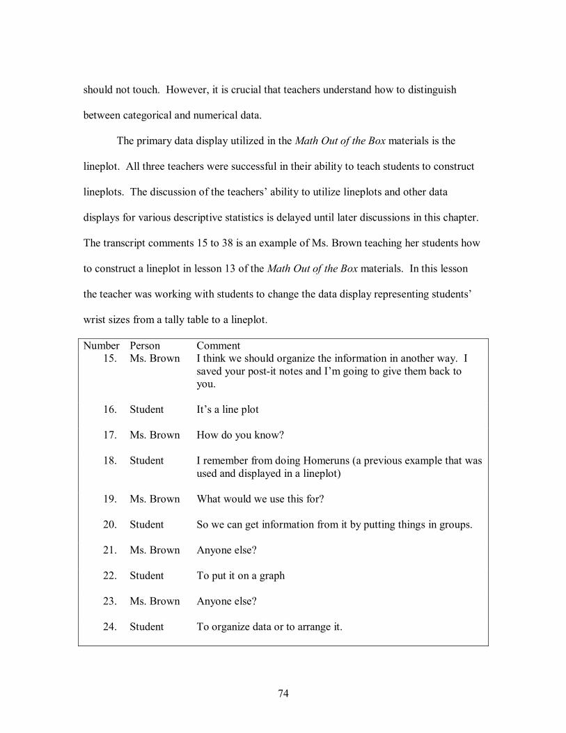
74

should not touch. However, it is crucial that teachers understand how to distinguish

between categorical and numerical data.

The primary data display utilized in the Math Out of the Box materials is the

lineplot. All three teachers were successful in their ability to teach students to construct

lineplots. The discussion of the teachers� ability to utilize lineplots and other data

displays for various descriptive statistics is delayed until later discussions in this chapter.

The transcript comments 15 to 38 is an example of Ms. Brown teaching her students how

to construct a lineplot in lesson 13 of the Math Out of the Box materials. In this lesson

the teacher was working with students to change the data display representing students�

wrist sizes from a tally table to a lineplot.

Number Person Comment 15. Ms. Brown I think we should organize the information in another way. I

saved your post-it notes and I�m going to give them back to you.

16. Student It�s a line plot

17. Ms. Brown How do you know?

18. Student I remember from doing Homeruns (a previous example that was used and displayed in a lineplot)

19. Ms. Brown What would we use this for?

20. Student So we can get information from it by putting things in groups.

21. Ms. Brown Anyone else?

22. Student To put it on a graph

23. Ms. Brown Anyone else?

24. Student To organize data or to arrange it.

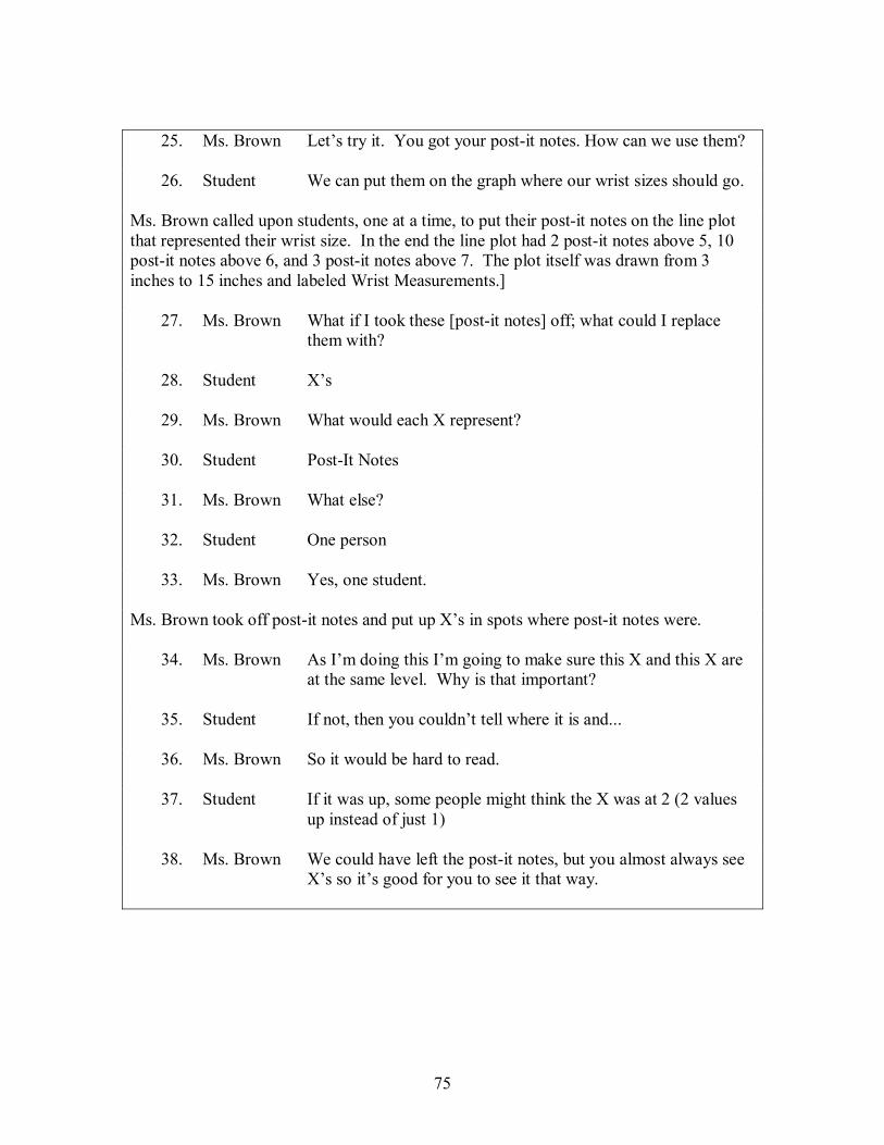
75

25. Ms. Brown Let�s try it. You got your post-it notes. How can we use them?

26. Student We can put them on the graph where our wrist sizes should go.

Ms. Brown called upon students, one at a time, to put their post-it notes on the line plot that represented their wrist size. In the end the line plot had 2 post-it notes above 5, 10 post-it notes above 6, and 3 post-it notes above 7. The plot itself was drawn from 3 inches to 15 inches and labeled Wrist Measurements.]

27. Ms. Brown What if I took these [post-it notes] off; what could I replace them with?

28. Student X�s

29. Ms. Brown What would each X represent?

30. Student Post-It Notes

31. Ms. Brown What else?

32. Student One person

33. Ms. Brown Yes, one student.

Ms. Brown took off post-it notes and put up X�s in spots where post-it notes were.

34. Ms. Brown As I�m doing this I�m going to make sure this X and this X are at the same level. Why is that important?

35. Student If not, then you couldn�t tell where it is and...

36. Ms. Brown So it would be hard to read.

37. Student If it was up, some people might think the X was at 2 (2 values up instead of just 1)

38. Ms. Brown We could have left the post-it notes, but you almost always see X�s so it�s good for you to see it that way.

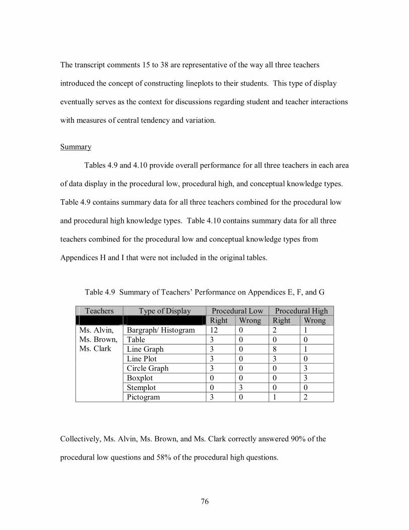
76

The transcript comments 15 to 38 are representative of the way all three teachers

introduced the concept of constructing lineplots to their students. This type of display

eventually serves as the context for discussions regarding student and teacher interactions

with measures of central tendency and variation.

Summary

Tables 4.9 and 4.10 provide overall performance for all three teachers in each area

of data display in the procedural low, procedural high, and conceptual knowledge types.

Table 4.9 contains summary data for all three teachers combined for the procedural low

and procedural high knowledge types. Table 4.10 contains summary data for all three

teachers combined for the procedural low and conceptual knowledge types from

Appendices H and I that were not included in the original tables.

Table 4.9 Summary of Teachers� Performance on Appendices E, F, and G

Teachers Type of Display Procedural Low Procedural High Right Wrong Right Wrong

Bargraph/ Histogram 12 0 2 1 Table 3 0 0 0 Line Graph 3 0 8 1 Line Plot 3 0 3 0 Circle Graph 3 0 0 3 Boxplot 0 0 0 3 Stemplot 0 3 0 0

Ms. Alvin, Ms. Brown, Ms. Clark

Pictogram 3 0 1 2

Collectively, Ms. Alvin, Ms. Brown, and Ms. Clark correctly answered 90% of the

procedural low questions and 58% of the procedural high questions.

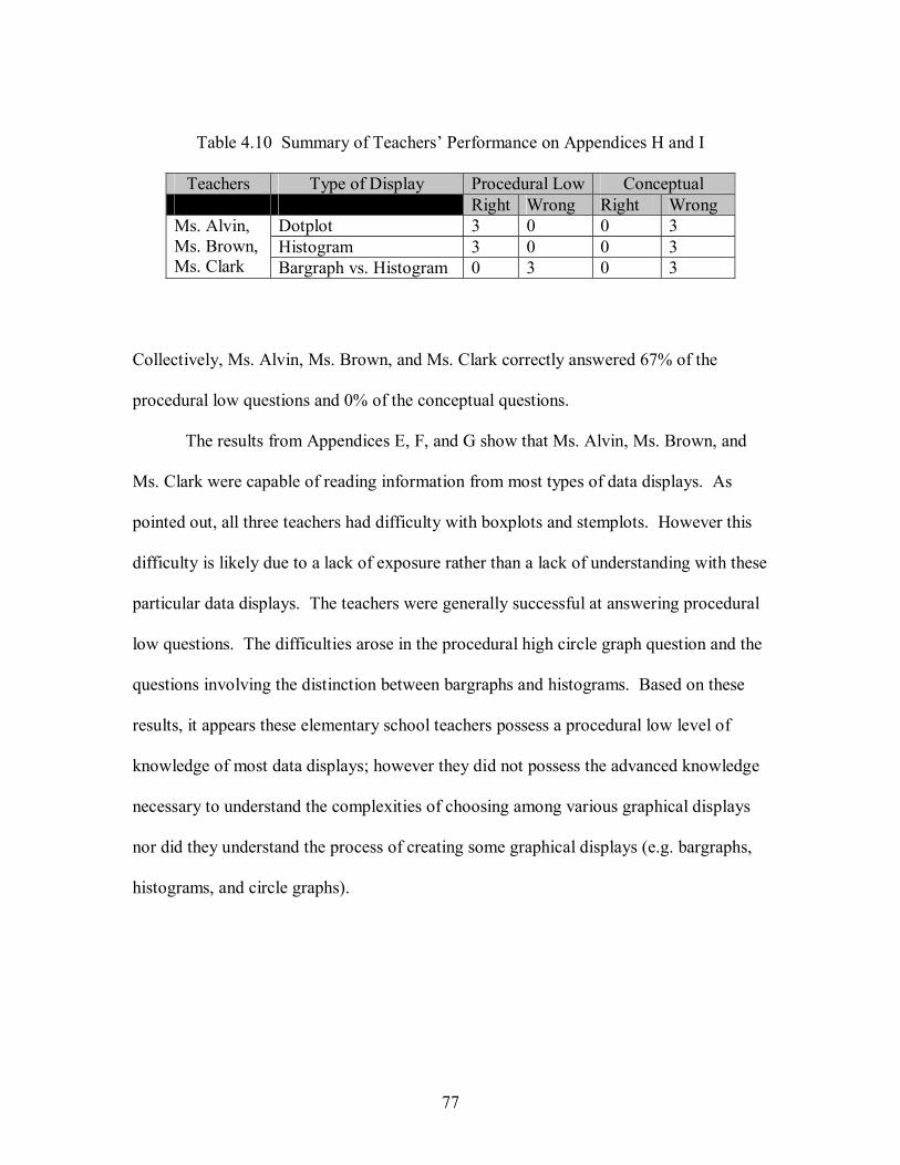
77

Table 4.10 Summary of Teachers� Performance on Appendices H and I

Teachers Type of Display Procedural Low Conceptual Right Wrong Right Wrong

Dotplot 3 0 0 3 Histogram 3 0 0 3

Ms. Alvin, Ms. Brown, Ms. Clark Bargraph vs. Histogram 0 3 0 3

Collectively, Ms. Alvin, Ms. Brown, and Ms. Clark correctly answered 67% of the

procedural low questions and 0% of the conceptual questions.

The results from Appendices E, F, and G show that Ms. Alvin, Ms. Brown, and

Ms. Clark were capable of reading information from most types of data displays. As

pointed out, all three teachers had difficulty with boxplots and stemplots. However this

difficulty is likely due to a lack of exposure rather than a lack of understanding with these

particular data displays. The teachers were generally successful at answering procedural

low questions. The difficulties arose in the procedural high circle graph question and the

questions involving the distinction between bargraphs and histograms. Based on these

results, it appears these elementary school teachers possess a procedural low level of

knowledge of most data displays; however they did not possess the advanced knowledge

necessary to understand the complexities of choosing among various graphical displays

nor did they understand the process of creating some graphical displays (e.g. bargraphs,

histograms, and circle graphs).

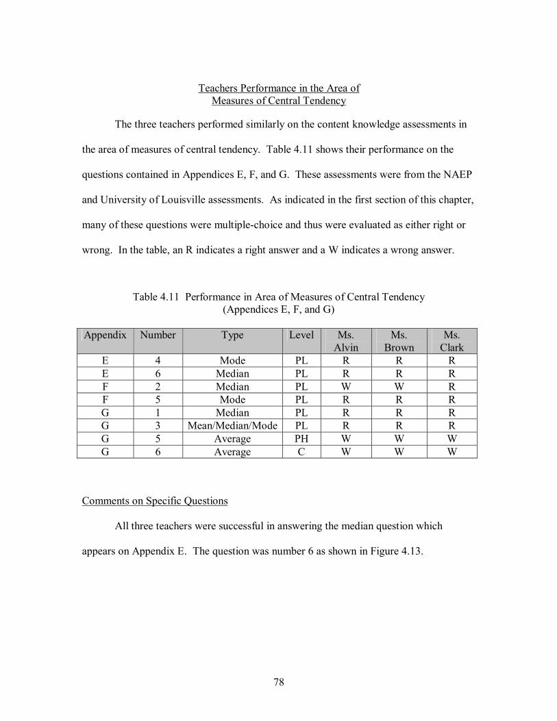
78

Teachers Performance in the Area of Measures of Central Tendency

The three teachers performed similarly on the content knowledge assessments in

the area of measures of central tendency. Table 4.11 shows their performance on the

questions contained in Appendices E, F, and G. These assessments were from the NAEP

and University of Louisville assessments. As indicated in the first section of this chapter,

many of these questions were multiple-choice and thus were evaluated as either right or

wrong. In the table, an R indicates a right answer and a W indicates a wrong answer.

Table 4.11 Performance in Area of Measures of Central Tendency (Appendices E, F, and G)

Appendix Number Type Level Ms.

Alvin Ms.

Brown Ms.

Clark E 4 Mode PL R R R E 6 Median PL R R R F 2 Median PL W W R F 5 Mode PL R R R G 1 Median PL R R R G 3 Mean/Median/Mode PL R R R G 5 Average PH W W W G 6 Average C W W W

Comments on Specific Questions

All three teachers were successful in answering the median question which

appears on Appendix E. The question was number 6 as shown in Figure 4.13.

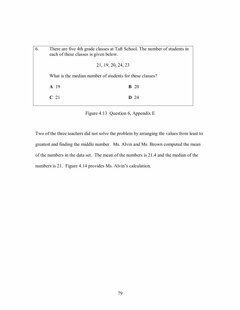
79

6. There are five 4th grade classes at Taft School. The number of students in each of these classes is given below.

21, 19, 20, 24, 23

What is the median number of students for these classes? A 19 B 20 C 21 D 24

Figure 4.13 Question 6, Appendix E

Two of the three teachers did not solve the problem by arranging the values from least to

greatest and finding the middle number. Ms. Alvin and Ms. Brown computed the mean

of the numbers in the data set. The mean of the numbers is 21.4 and the median of the

numbers is 21. Figure 4.14 provides Ms. Alvin�s calculation.

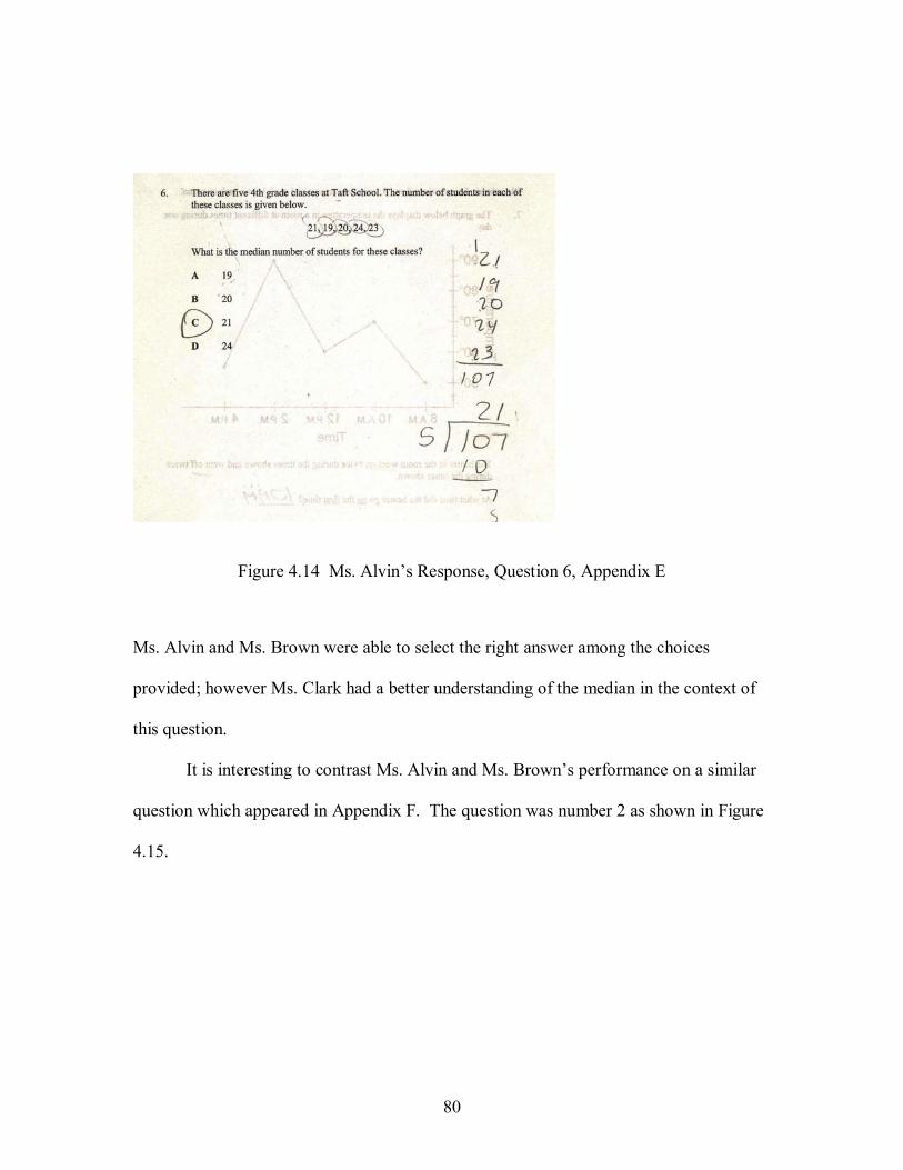
80

Figure 4.14 Ms. Alvin�s Response, Question 6, Appendix E

Ms. Alvin and Ms. Brown were able to select the right answer among the choices

provided; however Ms. Clark had a better understanding of the median in the context of

this question.

It is interesting to contrast Ms. Alvin and Ms. Brown�s performance on a similar

question which appeared in Appendix F. The question was number 2 as shown in Figure

4.15.

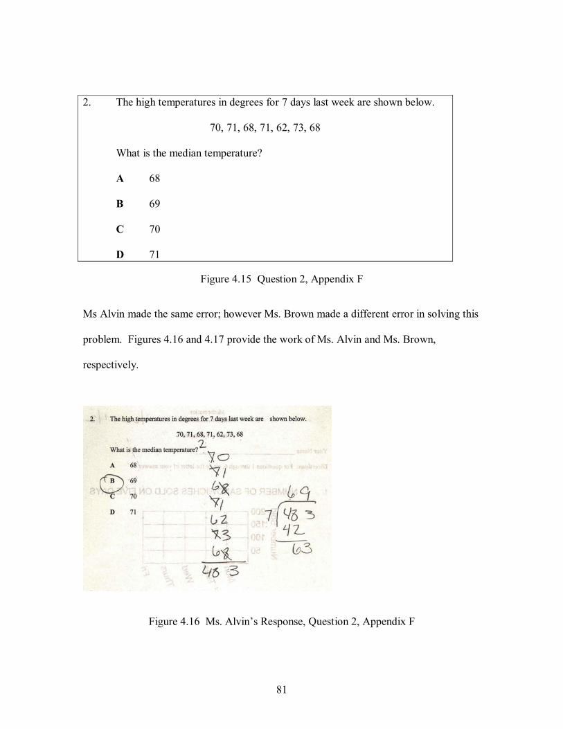
81

2. The high temperatures in degrees for 7 days last week are shown below.

70, 71, 68, 71, 62, 73, 68 What is the median temperature? A 68

B 69 C 70 D 71

Figure 4.15 Question 2, Appendix F

Ms Alvin made the same error; however Ms. Brown made a different error in solving this

problem. Figures 4.16 and 4.17 provide the work of Ms. Alvin and Ms. Brown,

respectively.

Figure 4.16 Ms. Alvin�s Response, Question 2, Appendix F

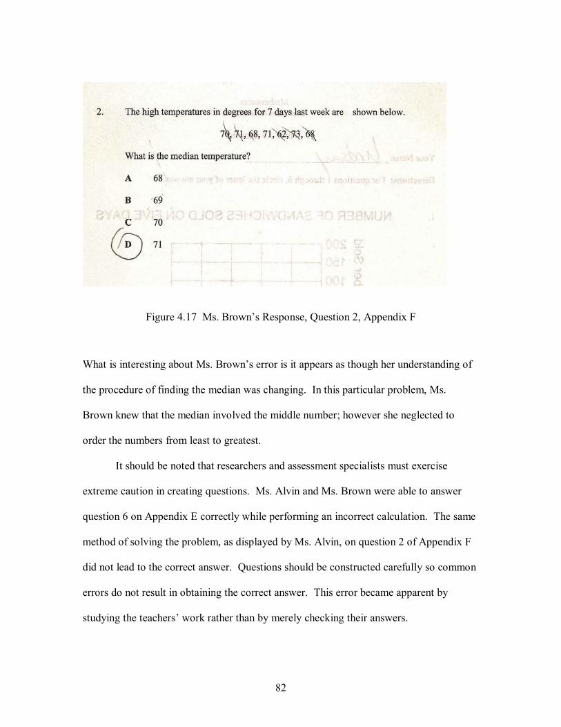
82

Figure 4.17 Ms. Brown�s Response, Question 2, Appendix F

What is interesting about Ms. Brown�s error is it appears as though her understanding of

the procedure of finding the median was changing. In this particular problem, Ms.

Brown knew that the median involved the middle number; however she neglected to

order the numbers from least to greatest.

It should be noted that researchers and assessment specialists must exercise

extreme caution in creating questions. Ms. Alvin and Ms. Brown were able to answer

question 6 on Appendix E correctly while performing an incorrect calculation. The same

method of solving the problem, as displayed by Ms. Alvin, on question 2 of Appendix F

did not lead to the correct answer. Questions should be constructed carefully so common

errors do not result in obtaining the correct answer. This error became apparent by

studying the teachers� work rather than by merely checking their answers.

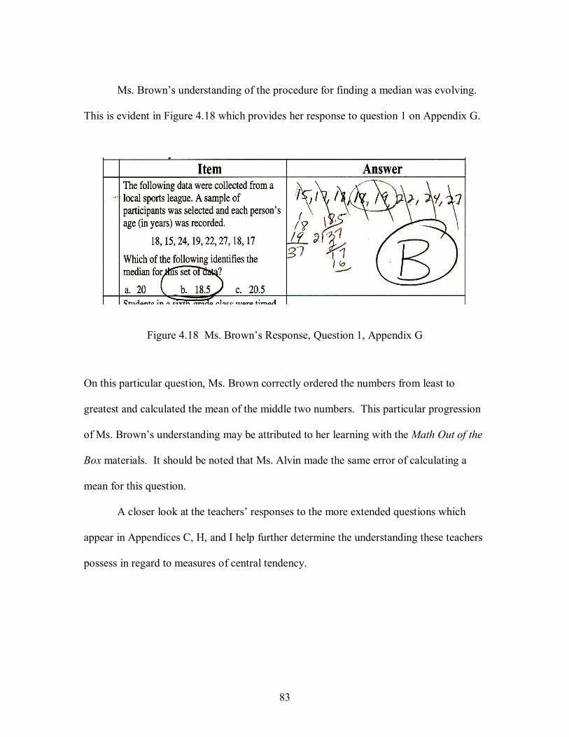
83

Ms. Brown�s understanding of the procedure for finding a median was evolving.

This is evident in Figure 4.18 which provides her response to question 1 on Appendix G.

Figure 4.18 Ms. Brown�s Response, Question 1, Appendix G

On this particular question, Ms. Brown correctly ordered the numbers from least to

greatest and calculated the mean of the middle two numbers. This particular progression

of Ms. Brown�s understanding may be attributed to her learning with the Math Out of the

Box materials. It should be noted that Ms. Alvin made the same error of calculating a

mean for this question.

A closer look at the teachers� responses to the more extended questions which

appear in Appendices C, H, and I help further determine the understanding these teachers

possess in regard to measures of central tendency.

84

Calculating the Mean, Median, and Mode

All three teachers were able to describe an appropriate method for determining the

mean, median, and mode. It was somewhat surprising that Ms. Alvin was able to provide

an appropriate description for finding the median, as it contrasted with her approach to

solving Questions 6, 2, and 1 on Appendices E, F, and G, respectively.

What is the difference between the Mean and the Median?

Two of the three teachers had difficulty explaining what these measures of center

actually represent. Ms. Clark indicated how to calculate such measures rather than

explaining what the measurements represent. An example of her response in regard to

the mean and median is shown in statements 39 to 42.

Number Person Comment 39. Researcher What does the mean represent?

40. Ms. Clark The mean is another word for average. So if you had the

numbers, 1,2,3,4,5, then the mean would be 1+2+3+4+5 divided by 5.

41. Researcher What does the median represent?

42. Ms. Clark The median is the middle number, so if the numbers were 1 through 5 the median would be 3.

Ms. Brown was confused regarding the difference between the two measures of center.

An example of her response in regard to the mean and median is shown in statements 43

to 50.

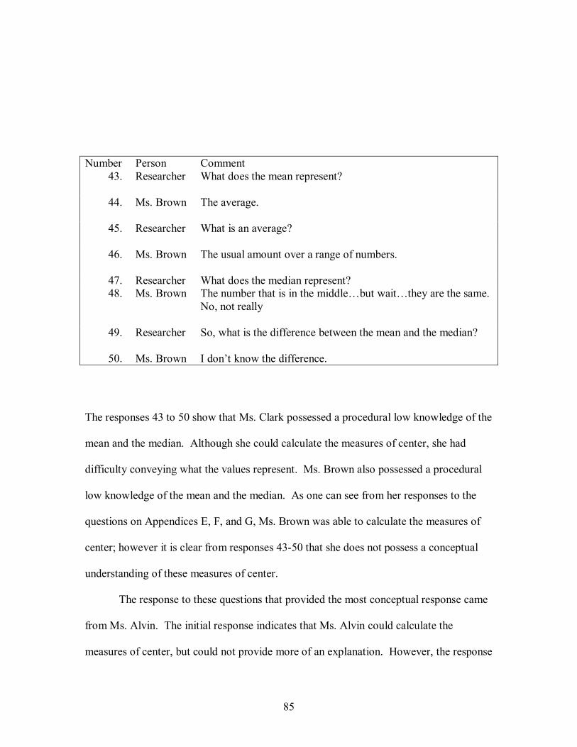
85

Number Person Comment 43. Researcher What does the mean represent?

44. Ms. Brown The average.

45. Researcher What is an average?

46. Ms. Brown The usual amount over a range of numbers.

47. Researcher What does the median represent? 48. Ms. Brown The number that is in the middle�but wait�they are the same.

No, not really

49. Researcher So, what is the difference between the mean and the median?

50. Ms. Brown I don�t know the difference.

The responses 43 to 50 show that Ms. Clark possessed a procedural low knowledge of the

mean and the median. Although she could calculate the measures of center, she had

difficulty conveying what the values represent. Ms. Brown also possessed a procedural

low knowledge of the mean and the median. As one can see from her responses to the

questions on Appendices E, F, and G, Ms. Brown was able to calculate the measures of

center; however it is clear from responses 43-50 that she does not possess a conceptual

understanding of these measures of center.

The response to these questions that provided the most conceptual response came

from Ms. Alvin. The initial response indicates that Ms. Alvin could calculate the

measures of center, but could not provide more of an explanation. However, the response

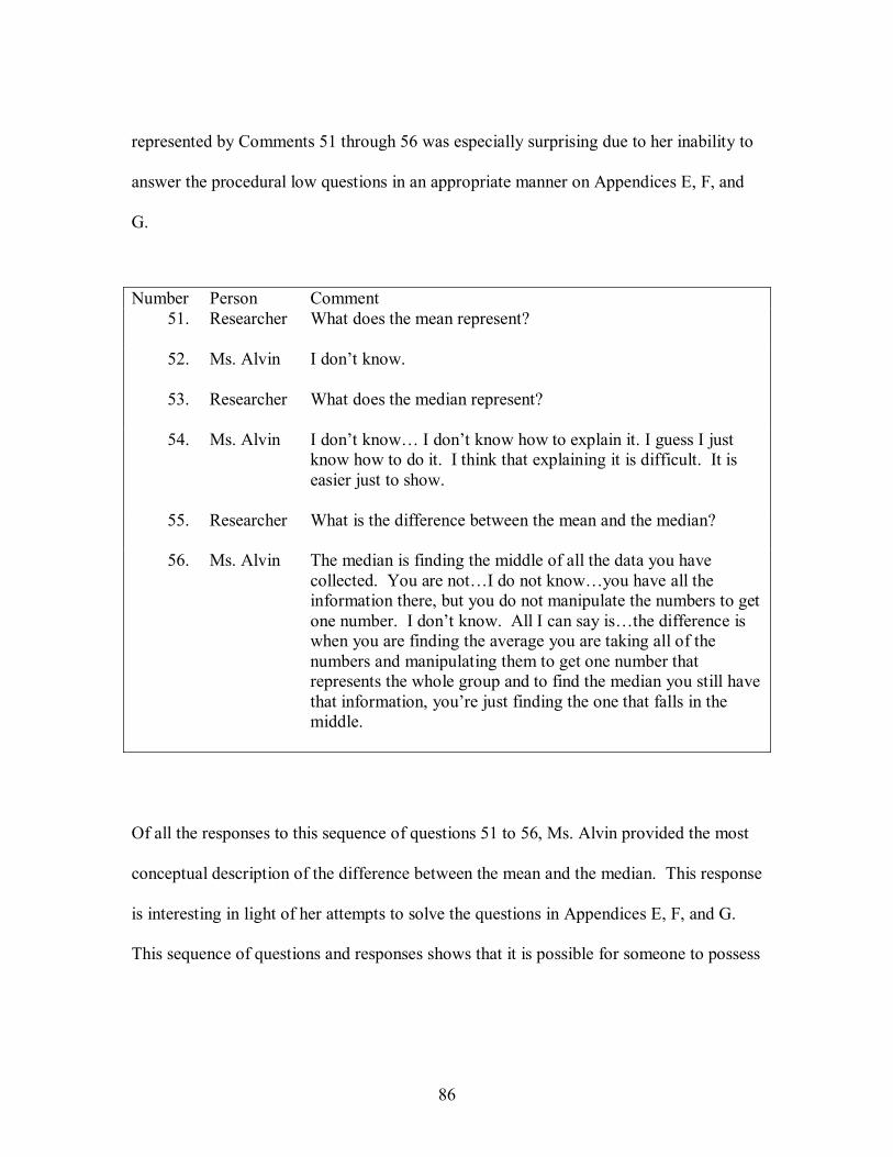
86

represented by Comments 51 through 56 was especially surprising due to her inability to

answer the procedural low questions in an appropriate manner on Appendices E, F, and

G.

Number Person Comment 51. Researcher What does the mean represent?

52. Ms. Alvin I don�t know.

53. Researcher What does the median represent?

54. Ms. Alvin I don�t know� I don�t know how to explain it. I guess I just

know how to do it. I think that explaining it is difficult. It is easier just to show.

55. Researcher What is the difference between the mean and the median?

56. Ms. Alvin The median is finding the middle of all the data you have collected. You are not�I do not know�you have all the information there, but you do not manipulate the numbers to get one number. I don�t know. All I can say is�the difference is when you are finding the average you are taking all of the numbers and manipulating them to get one number that represents the whole group and to find the median you still have that information, you�re just finding the one that falls in the middle.

Of all the responses to this sequence of questions 51 to 56, Ms. Alvin provided the most

conceptual description of the difference between the mean and the median. This response

is interesting in light of her attempts to solve the questions in Appendices E, F, and G.

This sequence of questions and responses shows that it is possible for someone to possess

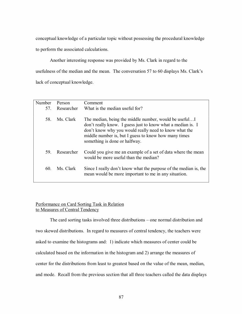
87

conceptual knowledge of a particular topic without possessing the procedural knowledge

to perform the associated calculations.

Another interesting response was provided by Ms. Clark in regard to the

usefulness of the median and the mean. The conversation 57 to 60 displays Ms. Clark�s

lack of conceptual knowledge.

Number Person Comment 57. Researcher What is the median useful for?

58. Ms. Clark The median, being the middle number, would be useful�I

don�t really know. I guess just to know what a median is. I don�t know why you would really need to know what the middle number is, but I guess to know how many times something is done or halfway.

59. Researcher Could you give me an example of a set of data where the mean would be more useful than the median?

60. Ms. Clark Since I really don�t know what the purpose of the median is, the mean would be more important to me in any situation.

Performance on Card Sorting Task in Relation to Measures of Central Tendency

The card sorting tasks involved three distributions � one normal distribution and

two skewed distributions. In regard to measures of central tendency, the teachers were

asked to examine the histograms and: 1) indicate which measures of center could be

calculated based on the information in the histogram and 2) arrange the measures of

center for the distributions from least to greatest based on the value of the mean, median,

and mode. Recall from the previous section that all three teachers called the data displays

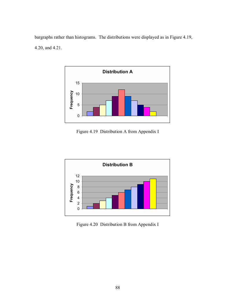
88

bargraphs rather than histograms. The distributions were displayed as in Figure 4.19,

4.20, and 4.21.

Distribution A

0

5

10

15

Freq

uenc

y

Figure 4.19 Distribution A from Appendix I

Distribution B

02468

1012

Freq

uenc

y

Figure 4.20 Distribution B from Appendix I

89

Distribution C

02468

1012

Freq

uenc

y

Figure 4.21 Distribution C from Appendix I

All three teachers indicated that measures of center could be found using these

distributions. However, only Ms. Clark was able to describe how to find the measures.

Comments 61 to 68 represent Ms. Clark�s description for finding the mean, median, and

mode.

Number Person Comment 61. Researcher Could you use the information in the displays to determine the

mean?

62. Ms. Clark I think I could do it; it might take a piece of paper. You had said they were on the same scale. If I knew these numbers I could calculate the mean by adding up all the values and dividing by the total amount.

63. Researcher Could you use the information in the displays to determine the median?

64. Ms. Clark Yes, I would list all the numbers and find the middle number.

65. Researcher Could you use the information in the displays to determine the mode?

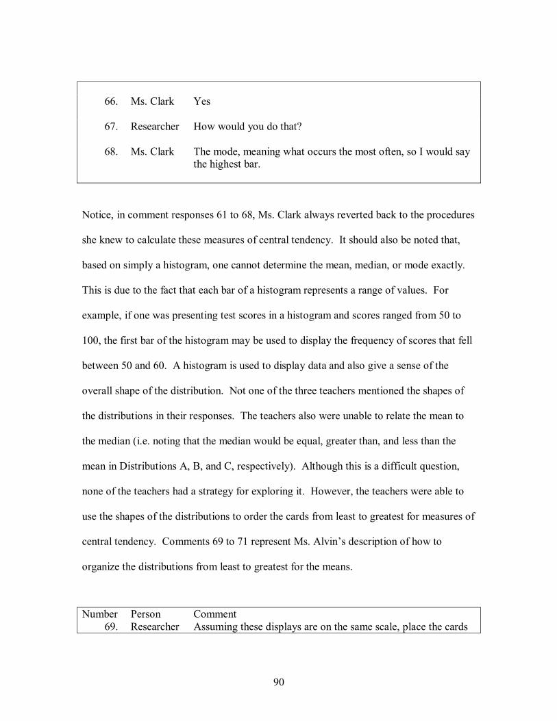
90

66. Ms. Clark Yes

67. Researcher How would you do that?

68. Ms. Clark The mode, meaning what occurs the most often, so I would say

the highest bar.

Notice, in comment responses 61 to 68, Ms. Clark always reverted back to the procedures

she knew to calculate these measures of central tendency. It should also be noted that,

based on simply a histogram, one cannot determine the mean, median, or mode exactly.

This is due to the fact that each bar of a histogram represents a range of values. For

example, if one was presenting test scores in a histogram and scores ranged from 50 to

100, the first bar of the histogram may be used to display the frequency of scores that fell

between 50 and 60. A histogram is used to display data and also give a sense of the

overall shape of the distribution. Not one of the three teachers mentioned the shapes of

the distributions in their responses. The teachers also were unable to relate the mean to

the median (i.e. noting that the median would be equal, greater than, and less than the

mean in Distributions A, B, and C, respectively). Although this is a difficult question,

none of the teachers had a strategy for exploring it. However, the teachers were able to

use the shapes of the distributions to order the cards from least to greatest for measures of

central tendency. Comments 69 to 71 represent Ms. Alvin�s description of how to

organize the distributions from least to greatest for the means.

Number Person Comment 69. Researcher Assuming these displays are on the same scale, place the cards

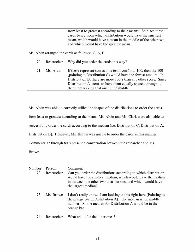
91

from least to greatest according to their means. So place these cards based upon which distribution would have the smallest mean, which would have a mean in the middle of the other two, and which would have the greatest mean.

Ms. Alvin arranged the cards as follows: C, A, B

70. Researcher Why did you order the cards this way?

71. Ms. Alvin If these represent scores on a test from 50 to 100, then the 100 (pointing at Distribution C) would have the fewest amount. In Distribution B, there are more 100�s than any other score. Since Distribution A seems to have them equally spaced throughout, then I am leaving that one in the middle.

Ms. Alvin was able to correctly utilize the shapes of the distributions to order the cards

from least to greatest according to the mean. Ms. Alvin and Ms. Clark were also able to

successfully order the cards according to the median (i.e. Distribution C, Distribution A,

Distribution B). However, Ms. Brown was unable to order the cards in this manner.

Comments 72 through 80 represent a conversation between the researcher and Ms.

Brown.

Number Person Comment 72. Researcher Can you order the distributions according to which distribution

would have the smallest median, which would have the median in between the other two distributions, and which would have the largest median?

73. Ms. Brown I don�t really know. I am looking at this right here (Pointing to the orange bar in Distribution A). The median is the middle number. So the median for Distribution A would be in the orange bar.

74. Researcher What about for the other ones?

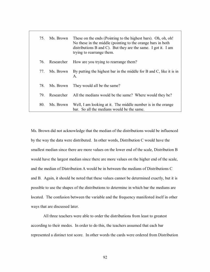
92

75. Ms. Brown These on the ends (Pointing to the highest bars). Oh, oh, oh!

No these in the middle (pointing to the orange bars in both distributions B and C). But they are the same. I got it. I am trying to rearrange them.

76. Researcher How are you trying to rearrange them?

77. Ms. Brown By putting the highest bar in the middle for B and C, like it is in A.

78. Ms. Brown They would all be the same?

79. Researcher All the medians would be the same? Where would they be?

80. Ms. Brown Well, I am looking at it. The middle number is in the orange bar. So all the medians would be the same.

Ms. Brown did not acknowledge that the median of the distributions would be influenced

by the way the data were distributed. In other words, Distribution C would have the

smallest median since there are more values on the lower end of the scale, Distribution B

would have the largest median since there are more values on the higher end of the scale,

and the median of Distribution A would be in between the medians of Distributions C

and B. Again, it should be noted that these values cannot be determined exactly, but it is

possible to use the shapes of the distributions to determine in which bar the medians are

located. The confusion between the variable and the frequency manifested itself in other

ways that are discussed later.

All three teachers were able to order the distributions from least to greatest

according to their modes. In order to do this, the teachers assumed that each bar

represented a distinct test score. In other words the cards were ordered from Distribution

93

C to Distribution A to Distribution B, since the highest bar in those distributions was

from lowest to highest on the scale. Again, this technically is incorrect because in a

histogram one cannot determine what those scores represent. For instance, in

Distribution C, although the highest bar appears on the lowest end of the scale, the mode

could actually be in one of the lower bars since what the mode is concerned with is the

specific value which occurs most often. It does not deal with which range of scores (i.e.

bar) that had the highest frequency. The teachers were unable to respond in this manner,

since they did not understand the differences between numerical and categorical data nor

did they understand the grouping that typically takes place in a histogram. Given their

understanding, their responses were viewed as if they understood the concept of the mode

in this particular context.

Summary

Based on the results from questions contained in Appendices E, F, G, and I, the

teachers demonstrated a procedural knowledge of measures of central tendency.

However, the teachers also showed weak conceptual knowledge in some areas of

measures of central tendency (e.g. Ms. Alvin�s description of the difference between the

mean and the median represented by comment number 56; all three teachers� ability to

order the distributions from least to greatest according to the means represented by Ms.

Alvin�s comments numbered 69-71). Some concepts involving measures of central

tendency follow in the next section focused on measures of variation. This is due to the

fact that a particular lesson that is used as an example involved more than just measures

of central tendency.

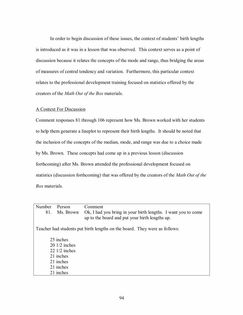
94

In order to begin discussion of these issues, the context of students� birth lengths

is introduced as it was in a lesson that was observed. This context serves as a point of

discussion because it relates the concepts of the mode and range, thus bridging the areas

of measures of central tendency and variation. Furthermore, this particular context

relates to the professional development training focused on statistics offered by the

creators of the Math Out of the Box materials.

A Context For Discussion

Comment responses 81 through 106 represent how Ms. Brown worked with her students

to help them generate a lineplot to represent their birth lengths. It should be noted that

the inclusion of the concepts of the median, mode, and range was due to a choice made

by Ms. Brown. These concepts had come up in a previous lesson (discussion

forthcoming) after Ms. Brown attended the professional development focused on

statistics (discussion forthcoming) that was offered by the creators of the Math Out of the

Box materials.

Number Person Comment 81. Ms. Brown Ok, I had you bring in your birth lengths. I want you to come

up to the board and put your birth lengths up.

Teacher had students put birth lengths on the board. They were as follows: 25 inches 20 1/2 inches 22 1/2 inches 21 inches 21 inches 21 inches 21 inches

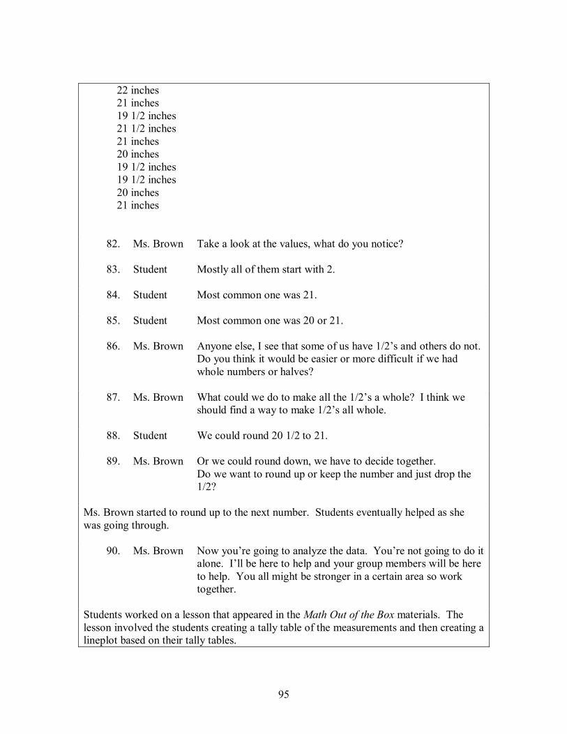
95

22 inches 21 inches 19 1/2 inches 21 1/2 inches 21 inches 20 inches 19 1/2 inches 19 1/2 inches 20 inches 21 inches

82. Ms. Brown Take a look at the values, what do you notice?

83. Student Mostly all of them start with 2.

84. Student Most common one was 21.

85. Student Most common one was 20 or 21.

86. Ms. Brown Anyone else, I see that some of us have 1/2�s and others do not. Do you think it would be easier or more difficult if we had whole numbers or halves?

87. Ms. Brown What could we do to make all the 1/2�s a whole? I think we should find a way to make 1/2�s all whole.

88. Student We could round 20 1/2 to 21.

89. Ms. Brown Or we could round down, we have to decide together. Do we want to round up or keep the number and just drop the 1/2?

Ms. Brown started to round up to the next number. Students eventually helped as she was going through.

90. Ms. Brown Now you�re going to analyze the data. You�re not going to do it alone. I�ll be here to help and your group members will be here to help. You all might be stronger in a certain area so work together.

Students worked on a lesson that appeared in the Math Out of the Box materials. The lesson involved the students creating a tally table of the measurements and then creating a lineplot based on their tally tables.

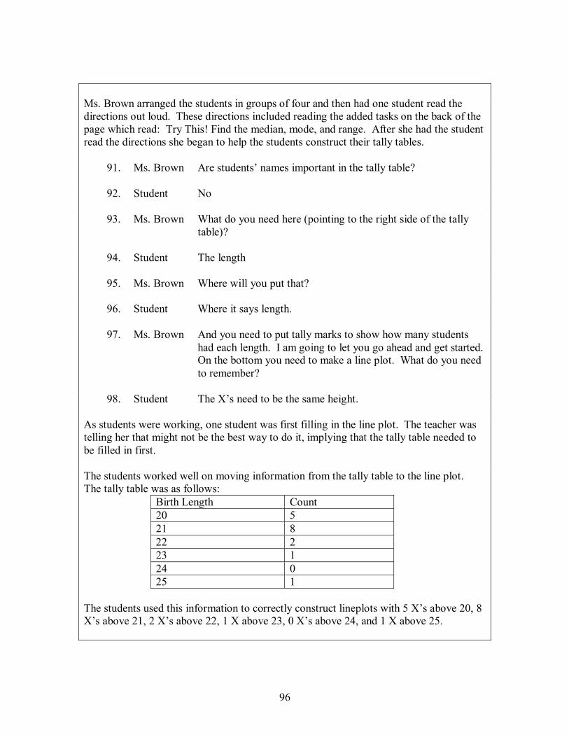
96

Ms. Brown arranged the students in groups of four and then had one student read the directions out loud. These directions included reading the added tasks on the back of the page which read: Try This! Find the median, mode, and range. After she had the student read the directions she began to help the students construct their tally tables.

91. Ms. Brown Are students� names important in the tally table?

92. Student No

93. Ms. Brown What do you need here (pointing to the right side of the tally table)?

94. Student The length

95. Ms. Brown Where will you put that?

96. Student Where it says length.

97. Ms. Brown And you need to put tally marks to show how many students had each length. I am going to let you go ahead and get started. On the bottom you need to make a line plot. What do you need to remember?

98. Student The X�s need to be the same height.

As students were working, one student was first filling in the line plot. The teacher was telling her that might not be the best way to do it, implying that the tally table needed to be filled in first. The students worked well on moving information from the tally table to the line plot. The tally table was as follows:

Birth Length Count 20 5 21 8 22 2 23 1 24 0 25 1

The students used this information to correctly construct lineplots with 5 X�s above 20, 8 X�s above 21, 2 X�s above 22, 1 X above 23, 0 X�s above 24, and 1 X above 25.

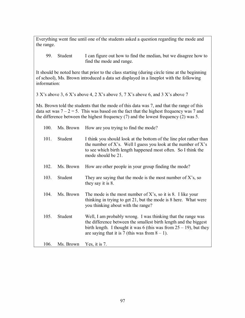
97

Everything went fine until one of the students asked a question regarding the mode and the range.

99. Student I can figure out how to find the median, but we disagree how to find the mode and range.

It should be noted here that prior to the class starting (during circle time at the beginning of school), Ms. Brown introduced a data set displayed in a lineplot with the following information: 3 X�s above 3, 6 X�s above 4, 2 X�s above 5, 7 X�s above 6, and 3 X�s above 7 Ms. Brown told the students that the mode of this data was 7, and that the range of this data set was 7 � 2 = 5. This was based on the fact that the highest frequency was 7 and the difference between the highest frequency (7) and the lowest frequency (2) was 5.

100. Ms. Brown How are you trying to find the mode?

101. Student I think you should look at the bottom of the line plot rather than the number of X�s. Well I guess you look at the number of X�s to see which birth length happened most often. So I think the mode should be 21.

102. Ms. Brown How are other people in your group finding the mode?

103. Student They are saying that the mode is the most number of X�s, so they say it is 8.

104. Ms. Brown The mode is the most number of X�s, so it is 8. I like your thinking in trying to get 21, but the mode is 8 here. What were you thinking about with the range?

105. Student Well, I am probably wrong. I was thinking that the range was the difference between the smallest birth length and the biggest birth length. I thought it was 6 (this was from 25 � 19), but they are saying that it is 7 (this was from 8 � 1).

106. Ms. Brown Yes, it is 7.

98

What is most interesting about this observation is that the concepts of the mode and range

came up during the professional development offered by creators of the Math Out of the

Box materials eight days prior to the teaching of this lesson. Even more interesting is that

when these concepts were introduced by a student during a lesson involving wrist sizes

only two days after the professional development, Ms. Brown corrected the students�

misconceptions.

Professional Development Training

Professional development training and what transpired in the class two days after

the training is described. Consider these descriptions in light of what occurred during the

lesson on birth lengths.

The context for the lesson introduced during the professional development was

the circumference of individuals� wrists from the materials. During this training, the

researcher sat at the table with Ms. Brown as she was participating in the professional

development. A line plot was constructed with four X�s above 6, eight X�s above 7, 9

X�s above 8, and 2 X�s above 9. During Ms. Brown�s exploration with the teachers, she

looked over at the researcher and indicated, �I know this stuff.� She proceeded to say

that the mode of the data was 9 and the range was 9 � 2 or 7. During the professional

development training, the correct method to find the mode and the range were discussed.

Ms. Brown clearly realized her error (i.e. using the frequencies rather than the values of

the variables) and by the end of the training focused on this topic indicated that the mode

was 8 inches and the range was 3 inches.

99

The Wrist Sizes Lesson Two Days Later

Recall the creation of the lineplot for students� wrist sizes as introduced by Ms.

Brown (comment numbers 15-38). Recall that the lineplot created during the wrist size

lesson had 2 X�s above 5, 10 X�s above 6, and 3 X�s above 7. During a discussion one of

the students in Ms. Brown�s class introduced the terminology of the range. Comments

107 through 150 are from a discussion that occurred between Ms. Brown and one of her

students following the construction of that lineplot.

Number Person Comment 107. Ms. Brown [To a particular student] You brought up a good word earlier.

What was that word?

108. Student Range

109. Ms. Brown What is the range?

110. Student Range is the difference between the biggest number of X�s and the smallest number of X�s.

111. Ms. Brown Anyone else?

112. Student Difference between the most popular and least popular.

113. Ms. Brown Can you show me?

The student showed that there were 10 X�s at 6 and 2 X�s at 7

114. Student So you take the 10 minus 2 to get a range of 8.

115. Ms. Brown Anyone else? How many number choices did we have when we recorded the information?

116. Student 15

117. Ms Brown How many measurements, in inches, did we actually have?

100

118. Student 3

119. Ms. Brown What measurement is the highest we used?

120. Student 6 inches

121. Ms. Brown Was that the highest number of inches that we used?

122. Student No. We used 7 as the highest.

123. Ms. Brown What was the smallest length?

124. Student 5

Ms. Brown wrote the word �Range� on the board with the numbers 7 and 5 beneath the word.

125. Ms. Brown I want to know the difference between these two numbers. What do I do?

126. Student Add them

127. Ms. Brown Close

128. Student Subtract them

129. Ms. Brown So, 7 � 5 = 2. Guess what that is.

130. Student The range.

131. Ms. Brown I made a mistake. Two what?

132. Student Inches

133. Ms. Brown So it is not the number of X�s. You just look down here (pointing to the numbers below the line in the lineplot).

134. Student I do not get how it is 7 and 5.

135. Ms. Brown We took the greatest number we had and the least.

136. Student We took the most before.

137. Student What about the mode?

101

138. Ms. Brown Let�s talk about the mode.

139. Student I think I know the mode. I think the mode is the opposite of the

range, so it is 7 + 5 = 12.

140. Student I think when you do the number of X�s, the highest amount of X�s is 10, so the mode would be 10.

141. Ms. Brown (Calling on a particular student) What did you say about the mode?

142. Student It would be the measurement that has the most X�s above it.

143. Ms. Brown What would that be?

144. Student 6 (The student went up to the board and pointed to it.)

145. Ms. Brown So what is the mode?

146. Student 6

147. Ms. Brown Did I have to add anything?

148. Student No

149. Ms. Brown I just have to say 6 inches. Did I have to count X�s?

150. Student You could just look at it.

During this sequence of events, Ms. Brown corrected the misconceptions introduced by

the students. This was the same misconception (comment number 110 for the range and

141 for the mode) that Ms. Brown exhibited during the professional development

training. However, just 6 days after this lesson was introduced and she corrected the

students� misconceptions, Ms. Brown reverted to her own misconceptions. It should be

noted that the student who went up to the board to correctly show that the mode of the

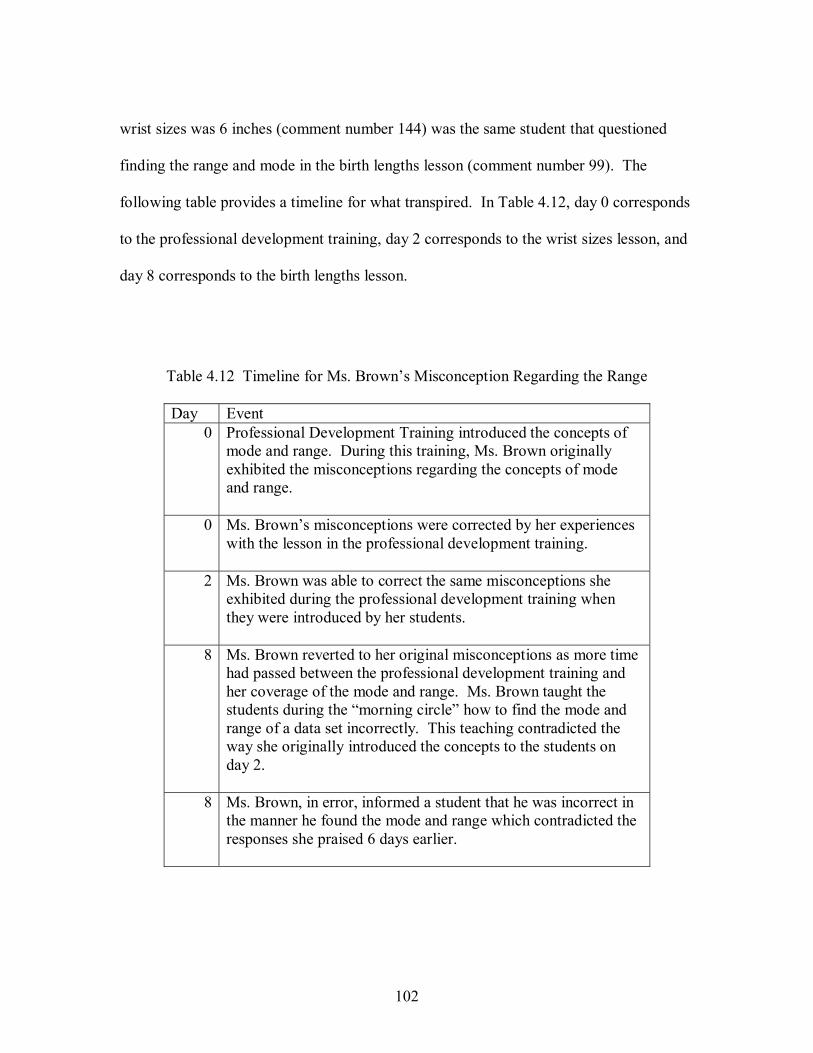
102

wrist sizes was 6 inches (comment number 144) was the same student that questioned

finding the range and mode in the birth lengths lesson (comment number 99). The

following table provides a timeline for what transpired. In Table 4.12, day 0 corresponds

to the professional development training, day 2 corresponds to the wrist sizes lesson, and

day 8 corresponds to the birth lengths lesson.

Table 4.12 Timeline for Ms. Brown�s Misconception Regarding the Range

Day Event 0 Professional Development Training introduced the concepts of

mode and range. During this training, Ms. Brown originally exhibited the misconceptions regarding the concepts of mode and range.

0 Ms. Brown�s misconceptions were corrected by her experiences with the lesson in the professional development training.

2 Ms. Brown was able to correct the same misconceptions she exhibited during the professional development training when they were introduced by her students.

8 Ms. Brown reverted to her original misconceptions as more time had passed between the professional development training and her coverage of the mode and range. Ms. Brown taught the students during the �morning circle� how to find the mode and range of a data set incorrectly. This teaching contradicted the way she originally introduced the concepts to the students on day 2.

8 Ms. Brown, in error, informed a student that he was incorrect in the manner he found the mode and range which contradicted the responses she praised 6 days earlier.

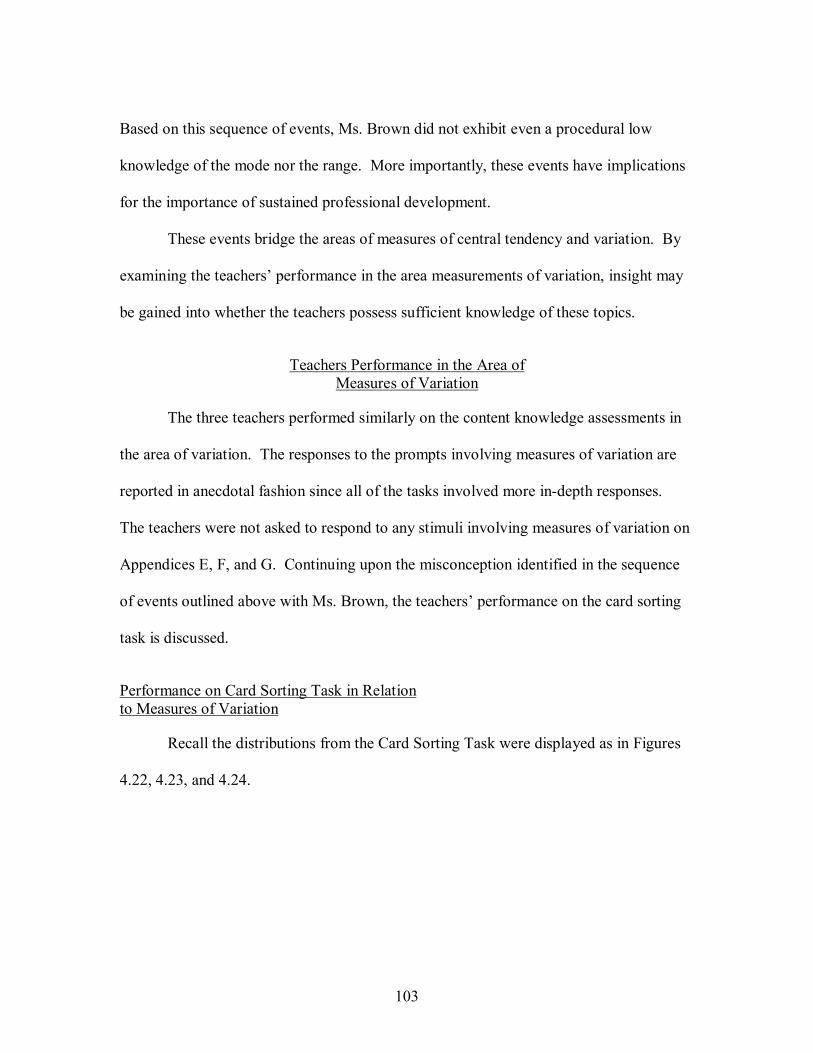
103

Based on this sequence of events, Ms. Brown did not exhibit even a procedural low

knowledge of the mode nor the range. More importantly, these events have implications

for the importance of sustained professional development.

These events bridge the areas of measures of central tendency and variation. By

examining the teachers� performance in the area measurements of variation, insight may

be gained into whether the teachers possess sufficient knowledge of these topics.

Teachers Performance in the Area of Measures of Variation

The three teachers performed similarly on the content knowledge assessments in

the area of variation. The responses to the prompts involving measures of variation are

reported in anecdotal fashion since all of the tasks involved more in-depth responses.

The teachers were not asked to respond to any stimuli involving measures of variation on

Appendices E, F, and G. Continuing upon the misconception identified in the sequence

of events outlined above with Ms. Brown, the teachers� performance on the card sorting

task is discussed.

Performance on Card Sorting Task in Relation to Measures of Variation

Recall the distributions from the Card Sorting Task were displayed as in Figures

4.22, 4.23, and 4.24.

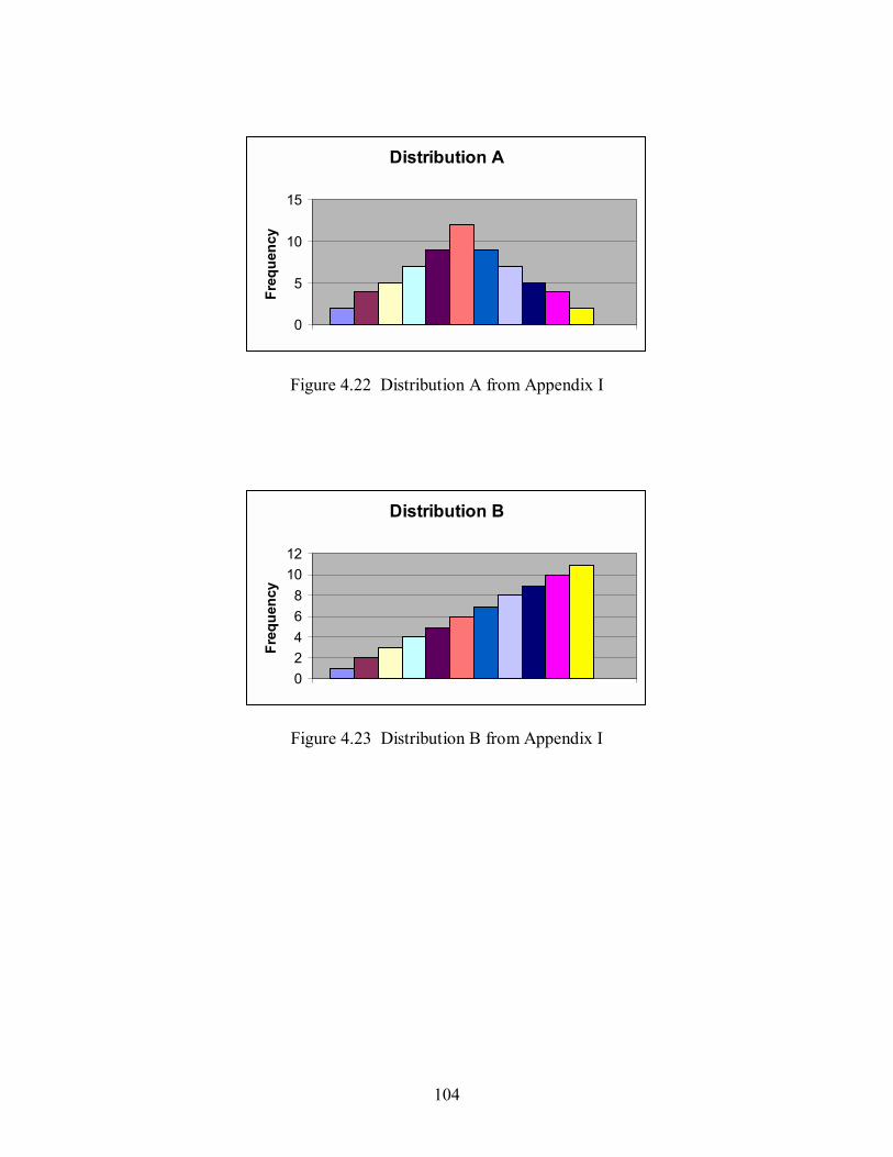
104

Distribution A

0

5

10

15

Freq

uenc

y

Figure 4.22 Distribution A from Appendix I

Distribution B

02468

1012

Freq

uenc

y

Figure 4.23 Distribution B from Appendix I

105

Distribution C

02468

1012

Freq

uenc

y

Figure 4.24 Distribution C from Appendix I

In regard to measures of variation, the teachers were asked to examine the histograms

and: 1) say which measures of variation could be calculated based on the information in

the histogram and 2) arrange the measures of variation for the distributions from least to

greatest based on the value of the range and standard deviation.

Ms. Alvin and Ms. Clark had not displayed the misconception involving the range

revealed by Ms. Brown in the previous sequence of events. However, during the Card

Sorting Task, all three teachers introduced the misconception of taking the difference

between the highest frequency and the lowest frequency in order to find the range. The

transcript comments 151 to 168 show how Ms. Clark revealed the misconception in the

context of arranging the distributions from least to greatest according to the range. The

initial lines in the transcript were from question 2 in Appendix I where Ms. Clark was

asked if she could use the data displays to find the range.

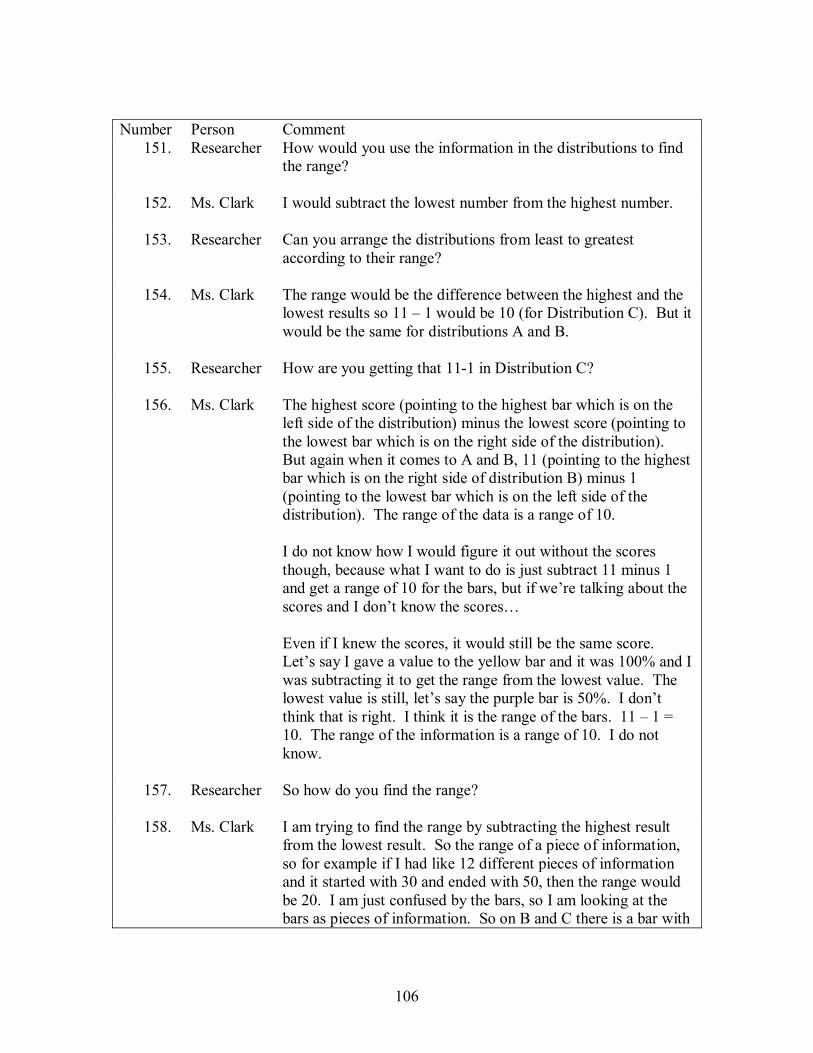
106

Number Person Comment 151. Researcher How would you use the information in the distributions to find

the range?

152. Ms. Clark I would subtract the lowest number from the highest number.

153. Researcher Can you arrange the distributions from least to greatest according to their range?

154. Ms. Clark The range would be the difference between the highest and the lowest results so 11 � 1 would be 10 (for Distribution C). But it would be the same for distributions A and B.

155. Researcher How are you getting that 11-1 in Distribution C?

156. Ms. Clark The highest score (pointing to the highest bar which is on the left side of the distribution) minus the lowest score (pointing to the lowest bar which is on the right side of the distribution). But again when it comes to A and B, 11 (pointing to the highest bar which is on the right side of distribution B) minus 1 (pointing to the lowest bar which is on the left side of the distribution). The range of the data is a range of 10. I do not know how I would figure it out without the scores though, because what I want to do is just subtract 11 minus 1 and get a range of 10 for the bars, but if we�re talking about the scores and I don�t know the scores� Even if I knew the scores, it would still be the same score. Let�s say I gave a value to the yellow bar and it was 100% and I was subtracting it to get the range from the lowest value. The lowest value is still, let�s say the purple bar is 50%. I don�t think that is right. I think it is the range of the bars. 11 � 1 = 10. The range of the information is a range of 10. I do not know.

157. Researcher So how do you find the range?

158. Ms. Clark I am trying to find the range by subtracting the highest result from the lowest result. So the range of a piece of information, so for example if I had like 12 different pieces of information and it started with 30 and ended with 50, then the range would be 20. I am just confused by the bars, so I am looking at the bars as pieces of information. So on B and C there is a bar with

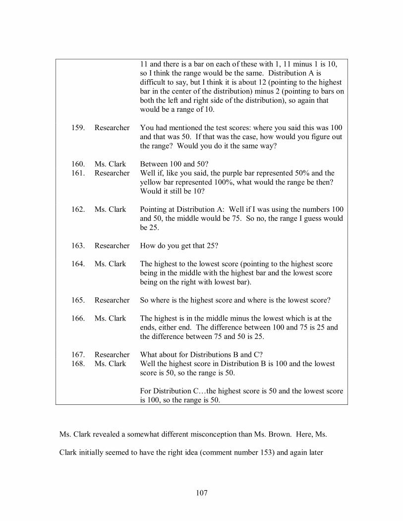
107

11 and there is a bar on each of these with 1, 11 minus 1 is 10, so I think the range would be the same. Distribution A is difficult to say, but I think it is about 12 (pointing to the highest bar in the center of the distribution) minus 2 (pointing to bars on both the left and right side of the distribution), so again that would be a range of 10.

159. Researcher You had mentioned the test scores: where you said this was 100 and that was 50. If that was the case, how would you figure out the range? Would you do it the same way?

160. Ms. Clark Between 100 and 50? 161. Researcher Well if, like you said, the purple bar represented 50% and the

yellow bar represented 100%, what would the range be then? Would it still be 10?

162. Ms. Clark Pointing at Distribution A: Well if I was using the numbers 100 and 50, the middle would be 75. So no, the range I guess would be 25.

163. Researcher How do you get that 25?

164. Ms. Clark The highest to the lowest score (pointing to the highest score being in the middle with the highest bar and the lowest score being on the right with lowest bar).

165. Researcher So where is the highest score and where is the lowest score?

166. Ms. Clark The highest is in the middle minus the lowest which is at the ends, either end. The difference between 100 and 75 is 25 and the difference between 75 and 50 is 25.

167. Researcher What about for Distributions B and C? 168. Ms. Clark Well the highest score in Distribution B is 100 and the lowest

score is 50, so the range is 50. For Distribution C�the highest score is 50 and the lowest score is 100, so the range is 50.

Ms. Clark revealed a somewhat different misconception than Ms. Brown. Here, Ms.

Clark initially seemed to have the right idea (comment number 153) and again later

108

(comment number 159). However, what she meant as the highest score was not the same

as what is typically thought of as the highest score. In reference to Distribution A (the

approximately normal distribution), Ms. Clark assigned the score of 75 to the bar in the

middle with scores of 50 and 100 on the ends. Here by highest, Ms. Clark meant the

mode (represented by the tallest bar), so she calculated 75 � 50 or 100 � 75 to obtain a

range of 25 rather than 50. When the same line of reasoning was used in reference to

Distributions B and C, Ms. Clark obtained the correct range of 50. Ms. Alvin exhibited a

similar misconception in her description of how to find the range.

All three teachers were unable to determine the standard deviations of the

distributions nor could they hypothesize which distribution would have a larger or

smaller standard deviation (the term spread was also used in an attempt to stimulate a

response). The teachers all indicated they had never been exposed to standard deviation

nor did they understand the concept. However, Ms. Clark correctly used the concept of

spread in responding to the catapult question as discussed in the following section.

Performance on the Catapult Question

The catapult question involved the teachers examining comparative dotplots in

order to choose the best catapult for landing ping pong balls within a certain band of a

target line for a game. The context was thoroughly explained to the teachers and they

were asked to explain the context back to the researcher, prior to their choosing a

catapult. The dotplots were displayed as in Figure 4.25.

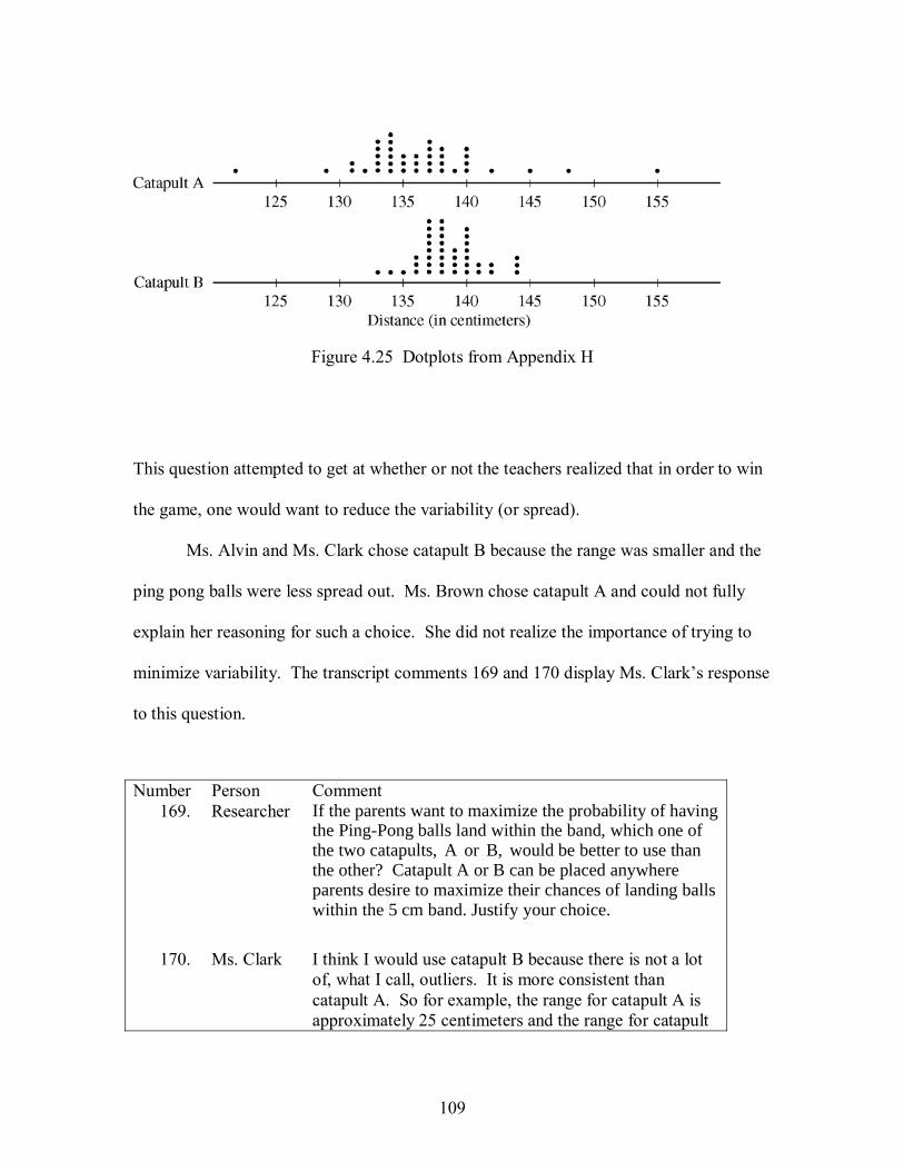
109

Figure 4.25 Dotplots from Appendix H

This question attempted to get at whether or not the teachers realized that in order to win

the game, one would want to reduce the variability (or spread).

Ms. Alvin and Ms. Clark chose catapult B because the range was smaller and the

ping pong balls were less spread out. Ms. Brown chose catapult A and could not fully

explain her reasoning for such a choice. She did not realize the importance of trying to

minimize variability. The transcript comments 169 and 170 display Ms. Clark�s response

to this question.

Number Person Comment 169. Researcher If the parents want to maximize the probability of having

the Ping-Pong balls land within the band, which one of the two catapults, A or B, would be better to use than the other? Catapult A or B can be placed anywhere parents desire to maximize their chances of landing balls within the 5 cm band. Justify your choice.

170. Ms. Clark I think I would use catapult B because there is not a lot

of, what I call, outliers. It is more consistent than catapult A. So for example, the range for catapult A is approximately 25 centimeters and the range for catapult

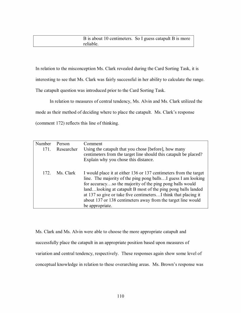
110

B is about 10 centimeters. So I guess catapult B is more reliable.

In relation to the misconception Ms. Clark revealed during the Card Sorting Task, it is

interesting to see that Ms. Clark was fairly successful in her ability to calculate the range.

The catapult question was introduced prior to the Card Sorting Task.

In relation to measures of central tendency, Ms. Alvin and Ms. Clark utilized the

mode as their method of deciding where to place the catapult. Ms. Clark�s response

(comment 172) reflects this line of thinking.

Number Person Comment 171. Researcher Using the catapult that you chose [before], how many

centimeters from the target line should this catapult be placed? Explain why you chose this distance.

172. Ms. Clark I would place it at either 136 or 137 centimeters from the target

line. The majority of the ping pong balls�I guess I am looking for accuracy�so the majority of the ping pong balls would land�looking at catapult B most of the ping pong balls landed at 137 so give or take five centimeters�I think that placing it about 137 or 138 centimeters away from the target line would be appropriate.

Ms. Clark and Ms. Alvin were able to choose the more appropriate catapult and

successfully place the catapult in an appropriate position based upon measures of

variation and central tendency, respectively. These responses again show some level of

conceptual knowledge in relation to these overarching areas. Ms. Brown�s response was

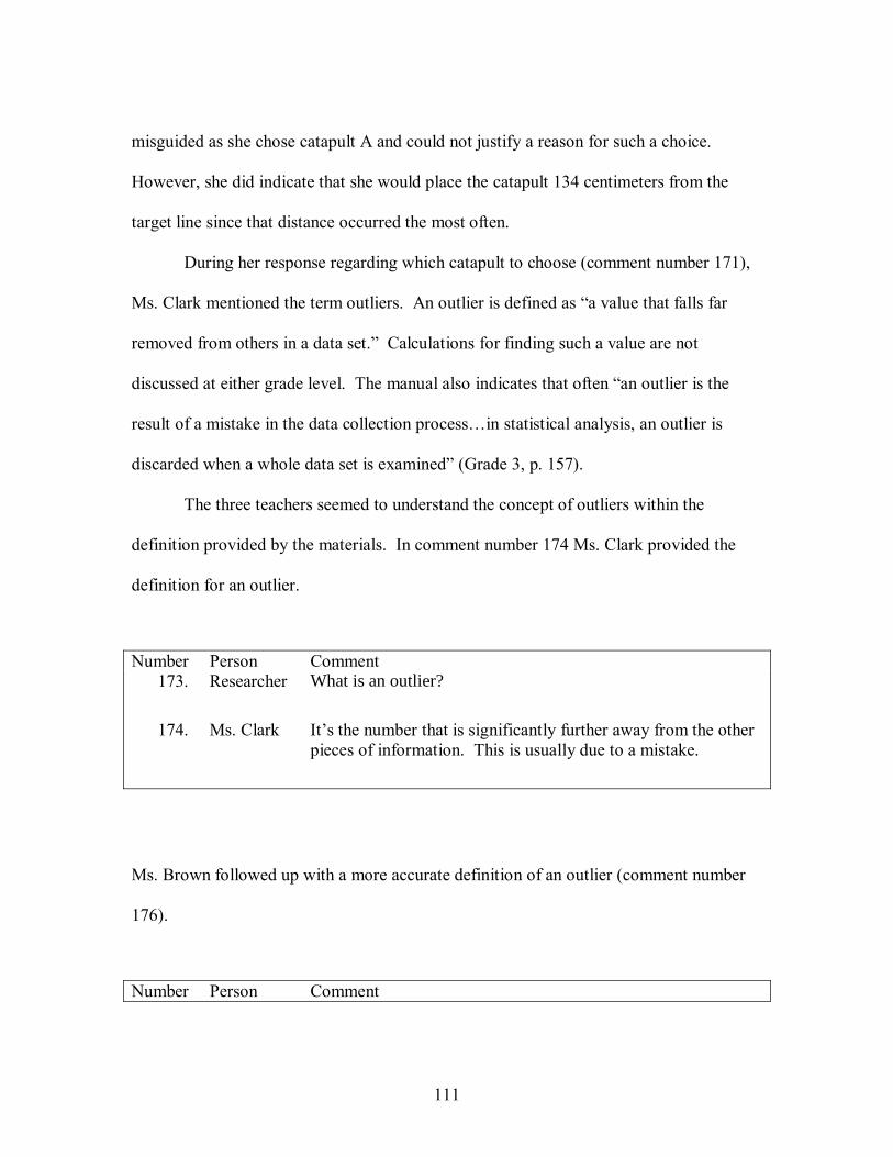
111

misguided as she chose catapult A and could not justify a reason for such a choice.

However, she did indicate that she would place the catapult 134 centimeters from the

target line since that distance occurred the most often.

During her response regarding which catapult to choose (comment number 171),

Ms. Clark mentioned the term outliers. An outlier is defined as �a value that falls far

removed from others in a data set.� Calculations for finding such a value are not

discussed at either grade level. The manual also indicates that often �an outlier is the

result of a mistake in the data collection process�in statistical analysis, an outlier is

discarded when a whole data set is examined� (Grade 3, p. 157).

The three teachers seemed to understand the concept of outliers within the

definition provided by the materials. In comment number 174 Ms. Clark provided the

definition for an outlier.

Number Person Comment 173. Researcher What is an outlier?

174. Ms. Clark It�s the number that is significantly further away from the other

pieces of information. This is usually due to a mistake.

Ms. Brown followed up with a more accurate definition of an outlier (comment number

176).

Number Person Comment

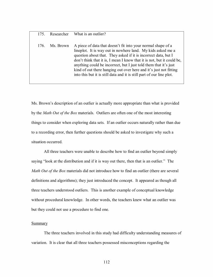
112

175. Researcher What is an outlier?

176. Ms. Brown A piece of data that doesn�t fit into your normal shape of a

lineplot. It is way out in nowhere land. My kids asked me a question about that. They asked if it is incorrect data, but I don�t think that it is, I mean I know that it is not, but it could be, anything could be incorrect, but I just told them that it�s just kind of out there hanging out over here and it�s just not fitting into this but it is still data and it is still part of our line plot.

Ms. Brown�s description of an outlier is actually more appropriate than what is provided

by the Math Out of the Box materials. Outliers are often one of the most interesting

things to consider when exploring data sets. If an outlier occurs naturally rather than due

to a recording error, then further questions should be asked to investigate why such a

situation occurred.

All three teachers were unable to describe how to find an outlier beyond simply

saying �look at the distribution and if it is way out there, then that is an outlier.� The

Math Out of the Box materials did not introduce how to find an outlier (there are several

definitions and algorithms); they just introduced the concept. It appeared as though all

three teachers understood outliers. This is another example of conceptual knowledge

without procedural knowledge. In other words, the teachers knew what an outlier was

but they could not use a procedure to find one.

Summary

The three teachers involved in this study had difficulty understanding measures of

variation. It is clear that all three teachers possessed misconceptions regarding the

113

concept of the range. Ms. Brown�s misconception in this area seems particularly deeply

rooted as exhibited by the reappearance of the misconception even after its correction. In

order to gauge what the teachers know and do not know it is important to return to what

the GAISE document recommends for students at Levels A and B. The GAISE

recommendations are compared to the results outlined above.

Connecting the Teachers� Understanding to the GAISE

Based upon the recommendations outlined by the GAISE document, it would

appear that the three teachers involved in this study were not prepared to help students

realize the objectives of Levels A and B. The teachers did not possess an adequate level

of knowledge of the topics expected of students at Levels A and B. In order to elaborate

upon this statement, topics in the areas of data displays, measures of central tendency,

and measures of variation are discussed.

Data Displays

The GAISE document indicates that students at Level A should understand how

to construct and use frequency tables, bargraphs, stem-and-leaf plots, dotplots,

scatterplots, and timeplots. The teachers in this study had not been exposed to stem-and-

leaf plots or scatterplots. This was exhibited by their performance on questions 2 and 5

on Appendix G. Dotplots are considered extremely similar to lineplots and the teachers

seemed to have a good understanding of those data displays based on their experience

with the Math Out of the Box materials.

114

The GAISE document indicates that it is important for students to realize the

difference between a bargraph and histogram at Level A. Based on the teachers�

responses to various questions (e.g. comment numbers 1-8), it appears that they did not

possess such knowledge. This type of knowledge would be considered as conceptual.

Teachers should understand the difference between categorical and numerical data and

should realize what is an appropriate data display for each. Based on the results of this

study, these three elementary school teachers were not prepared to help their students

make these realizations.

At Level B, students should understand how to construct and use histograms,

frequency tables, boxplots, grouped frequency tables, and time series plots. Based on the

results of this study, these teachers were unfamiliar with histograms and boxplots. They

were unable to answer question 6 on Appendix G based on their lack of familiarity with

boxplots. Students at this level should also be introduced to the misuses of graphs.

Possessing the high level of procedural knowledge necessary to construct a circle graph

(as appears on question 8 of Appendix G) is related to the ability to determine if graphs

are misused. If one cannot appropriately construct a data display, then it may be assumed

that same person would have difficulty in determining if a data display misrepresents the

information. It is important when constructing any data display to make sure the display

is representative of the data involved. An inability to comprehend what appears in

various data displays influences students� abilities to find appropriate measures of central

tendency.

115

Measures of Central Tendency

At Level A, students are expected to understand the mean, median, and mode as a

fair share, middle point, and value that occurs most often, respectively. Based on the

results of this study, these three teachers did not understand the mean and mode. The

teachers were able to calculate the mean; however two of the three teachers were unable

to realize the mean represents a fair share. Ms. Alvin was the only teacher that was able

to provide a description of the mean that included the idea that the mean is a fair share

(comment numbers 51-56). This is exhibited by their inability to determine when a mean

was more useful than a median.

Students at Level A should be able to determine when certain measures of central

tendency are inappropriate for different data sets. A lack of understanding of the

appropriateness of various measures of central tendency is apparent in Ms. Clark�s

response to when a median may be more useful than a mean (comment numbers 57-60).

Measures of Variation

These three teachers seemed most ill-prepared in the area of variation. At Level

A, students should understand what maximum and minimum values represent and how

these values relate to the range for a set of data. It is clear from the results of the study

that the teachers did not understand the concept of the range, or at least were not able to

apply what they knew to a histogram with an undefined independent variable. In fact, all

three teachers revealed misconceptions in regard to finding the range for a set of data. At

Level A, students should also begin to question why variations occur in data (e.g.

outliers). Based on their interaction with the Math Out of the Box materials, it appears

116

that the teachers knew what an outlier is, but they did not realize the importance of

investigating outliers further. This is related to the definition presented in the materials

themselves. However, Ms. Brown seemed to have the beginnings of such an

understanding.

At Level B, students should begin to realize variation involves comparing values

to a central value. Based on the results of this study, these three teachers had not made

such a realization. According to the results involving the determination of the spread for

the card sorting tasks, the teachers were unable to relate how these distributions may be

spread about a central value. The GAISE document also recommends that students at

Level B be introduced to the interquartile range. Given the teachers� lack of knowledge

in reference to the range, it is safe to assume they did not possess the knowledge of the

interquartile range.

Summary

Based on the results of this study it would appear that the three teachers involved

in this study were not prepared to help students realize the objectives of Levels A and B

as outlined in the GAISE document. It is unreasonable to expect teachers to teach

students material at a level which exceeds their own level of knowledge. In the next

section of this chapter, the influence these experiences had on the teachers� awareness of

their knowledge in the area of statistics is discussed.

117

Teachers� Awareness of Their Understanding

All three teachers had some reservations about teaching mathematics in general.

In relation to data analysis and statistical topics, the teachers felt fairly comfortable

teaching material at their grade level. However, they were hesitant to consider

themselves ready to teach anything beyond their grade level. This feeling is evident in

the transcript comment numbers 177 and 178.

Number Person Comment 177. Researcher How would you assess your level of understanding of data

analysis and statistical topics covered at your grade level?

178. Ms. Clark I feel comfortable teaching the material at the third grade level, but I wouldn�t want to go up to the fourth grade level. Students have difficulty with the concepts. I understand data at this level and feel comfortable teaching the students.

These feelings were echoed by Ms. Alvin and Ms. Brown. They all felt comfortable

teaching the material at their particular level, but not beyond.

Through their experiences with the Math Out of the Box materials, the teachers

became exposed to more data analysis and statistical topics than they had in the past. As

a result, they had to learn or re-learn some of the material. This is evident in the

transcript comment numbers 170 to 180.

Number Person Comment 179. Researcher What concepts did you have to review prior to teaching the data

analysis and statistical lessons?

118

180. Ms. Alvin I had to review all of the material: mean, median, mode, range.

I had never heard of an outlier before. We never covered this kind of stuff before these materials. I mean�in science, we may have done an activity where we counted the number of seeds in a bean pod. We may have talked about what number occurred most often. We didn�t teach enough of it, so I hadn�t thought about this stuff for a long time.

It is clear that Ms. Alvin was not the only teacher who had a change in view regarding the

knowledge necessary to teach data analysis and statistics. Transcript comments 181

through 182 represent comments from a conversation between the researcher and Ms.

Clark.

Number Person Comment 181. Researcher Has your thinking about data analysis and statistics changed as

a result of the Math Out of the Box lessons?

182. Ms. Clark Definitely, because I didn�t even know most of these terms. I knew what a mean or a mode was, but there were things that I didn�t even understand. I had only been given a shallow amount of data before. This presented it within a context so it wasn�t just numbers. It had more meaning to it, than just doing it. There were a lot of levels that you could go all over with.

Ms. Brown also developed a realization that there was a lot more to learn when it came to

mathematics as shown in transcript comments 183 through 184.

Number Person Comment

119

183. Researcher What have you learned about data analysis and statistics as a result of your work with the Math Out of the Box materials?

184. Ms. Brown That I�m not that good at it, but it�s OK because my kids can help me through it and it�s OK that if I don�t know something I can learn it with my students. We can all learn it together.

This quote has two views that can be taken. On the one hand, it can be seen as a negative

that a teacher would think of entering a classroom without knowing the material. On the

other hand, it can be seen as a positive, that at least this teacher is willing to learn new

things with her students. As the sophistication level involved in standards are increased

and teachers have not experienced the learning of concepts firsthand, they will need time

to learn the material.

Ms. Clark made a similar comment as shown in comments 185 through 186.

Number Person Comment 185. Researcher What have you learned about yourself as a learner?

186. Ms. Brown That I am capable too. I learned a lot that I didn�t know before.

I mean it is third grade math but I still didn�t necessary know all of it or experience all of it and do it.

Based on these limited results, it does appear that the teachers gained more of an

awareness of where their knowledge was in regard to statistics. It should be noted that

their feelings were also influenced by the questions that the researcher posed. Based on

120

these questions, the teachers felt as though they were not prepared at the level suggested

in the GAISE document.

The most telling result in regard to the teachers� awareness of their knowledge

comes from the results of a question which was taken from the Begg and Edwards (1999)

study. At the beginning and end of the study, the teachers were asked the following

question:

If you could receive a day of professional development focused on data analysis

and statistical topics, would you prefer to have the professional development focused on:

(a) activities at your grade level; or (b) data analysis and statistical content? At the

beginning of the study, all three teachers chose professional development focused on

activities. At the end of the study, all three teachers chose professional development

focused on data analysis and statistical content. As a follow-up question to this change in

opinion, all the teachers were asked whether their change was due more to their

interaction with the Math Out of the Box materials or with their interaction with the

questions posed on various assessments that were part of this study. All three teachers

indicated their change was due more to their interaction with the questions and their self-

discovered lack of familiarity with many data analysis and statistical topics.

Conclusion

The results of this study indicate that these elementary school teachers were not

prepared to teach the level of detail associated with the GAISE document. Based on

these results, these teachers primarily had a procedural low level of knowledge in the area

121

of statistics. There are several implications to this study and further questions for

consideration that are discussed in the next chapter.

122

CHAPTER FIVE

IMPLICATIONS

This chapter discusses the implications that may be drawn from this study. The

chapter is divided into six sections. The first section provides a short synopsis of the

answers to the research questions. The second section focuses on the difference between

procedural and conceptual knowledge in the area of statistics. The third section discusses

the implications for teacher training. The fourth section focuses on the importance of

sustained professional development. The fifth section discusses curricular implications.

The chapter concludes with the identification of topics and questions for future research.

Answering the Research Questions

This research study attempted to answer the following research questions:

1. What is the understanding of elementary school teachers in the following

areas of statistics: data displays, measures of central tendency, and measures

of variation?

2. Does the implementation of the curricula materials and exposure to advanced

assessment instruments influence elementary school teachers� awareness of

their understanding of statistics?

Based on the results of this study, it is possible to provide answers to the research

questions. The answers provided in this section are brief but are expanded upon

throughout the chapter. The elementary school teachers involved in this study generally

had a low-level (procedural low) understanding of essential topics in statistics. Their

123

understanding was lacking in each area explored during the course of this study. The

teachers� interaction with the Math Out of the Box materials and exposure to advanced

assessment instruments influenced their awareness of their understanding. By the end of

the study, the teachers had realized they lacked the sophisticated level of understanding

that is necessary to teach statistics effectively. The answer to question 1 is expanded

upon in Section 2 and the answer to question 2 is expanded upon in Section 4.

Procedural versus Conceptual Knowledge of Essential Topics in Statistics

As described previously, it is difficult to define �understanding of statistical

content.� The results of this study help shape a distinction between what it means to

understand certain statistical topics at the procedural versus the conceptual level. Based

on this study, these distinctions can be made in the areas of data displays, measures of

central tendency, and measures of variation.

In the area of data displays, teachers should, according to the GAISE document,

recognize the advantages and disadvantages of various data displays. This recognition

represents conceptual knowledge; however the teachers in this study rarely exhibited this

type of knowledge. The ability to read information from a particular display involves a

procedural knowledge of that particular display. The teachers involved in this study were

all able to use the information in tables, bargraphs, lineplots, dotplots, linegraphs, and

pictograms to answer particular questions. However, not one of the teachers was able to

understand the conceptual basis for the appropriateness of certain data displays for

particular sets of data.

124

The appropriateness of various data displays for particular sets of data is

dependent on whether the variable is categorical or numerical. The teachers involved in

this study were misguided in their focus. In the birth lengths setting, for example, Ms.

Brown focused on the frequency for each birth length rather than the birth lengths

themselves. She did not distinguish between the value of the variable (the actual length)

and the number of times that particular value occurred. This inability to identify what the

variable was led to her misconception regarding the mode and range. In order for

teachers to develop conceptual knowledge in regard to data displays, they must

understand that the variable of interest should determine the appropriate types of data

displays. Elementary school teachers with a conceptual understanding of data displays

should realize that there are appropriate displays for categorical data (e.g. frequency

tables, bargraphs, and circle graphs) and appropriate, but different, displays for numerical

data (e.g. histograms, stemplots, boxplots). The elementary school teachers in this study

did not possess such an understanding. While they had procedural knowledge in that

they could answer questions that required them to read information from graphs, they did

not possess conceptual knowledge that would allow them to realize the appropriateness of

different data displays for certain situations.

In the area of measures of central tendency, there is also a distinction between

procedural and conceptual knowledge. Although Ms. Alvin had difficulty with the

procedure of finding a median at times, overall these three teachers were successful in

applying the procedures to find the mean, median, and mode. However, Ms. Alvin was

125

the only teacher that was able to describe some of the properties that make the mean and

the median different.

For conceptual knowledge in the area of measures of central tendency, teachers

should understand the appropriateness and usefulness of the mean, median, and mode.

They should also realize that the appropriateness and usefulness of the mean, median, and

mode are connected to whether the data is categorical or numerical. Of the three, the

mode is the only useful measure of central tendency for categorical data. For example,

when considering the religion associated with a particular area, it would only be

appropriate to report the mode. The mode for this particular situation would be the

religion that was represented most often. It would not be appropriate to calculate the

mean or find the median of Buddhism, Christianity, Hinduism, Islam, Judaism, and the

many other religions around the world.

In order for elementary school teachers to possess conceptual knowledge of

measures of central tendency related to numerical data, they should realize that the

appropriateness and usefulness of the median and mean are connected to measures of

variation. In regard to the median, teachers� understanding should begin with the

realization that the median is the middle value when all values are arranged from least to

greatest. Their understanding of the median should extend to their realization that it is

the value that has the smallest absolute distance from all other values in the data set as

compared with any other data point. Consider the following data set to examine this

property.

126

1, 4, 5, 9, 14

The median of this data set is 5. This value has the smallest absolute distance (18) from

all other values. The absolute distance for 1 is .2814191514111 =−+−+−+−+−

The absolute distance for 4 is .1914494544414 =−+−+−+−+− The absolute

distance for 5 is .1814595554515 =−+−+−+−+− The absolute distance for 9

is .2214999594919 =−+−+−+−+− The absolute distance for 14 is

.371414914514414114 =−+−+−+−+− The smallest absolute distance (18 for

this example) occurs at the median. Elementary school teachers who possess a

conceptual understanding of the median should realize that the median has this property.

In regard to the mean, elementary school teachers should realize the mean is the

balance point of the data. Because of this the mean is influenced by extreme values.

Teachers should realize the reason for this is that the mean involves all values in a data

set where as the median only involves the one particular value that falls in the middle. To

illustrate this, consider a slightly modified data set from the one provided in the previous

example.

1, 4, 5, 9, 140

The median of this data set is 5, which is the same as the median in the previous example.

The mean of the original data set (1, 4, 5, 9, 14) is 6.6 whereas the mean of this new data

set is 31.8. The influence of one extreme value on the mean may be drastic. As a result,

in order for elementary school teachers to possess conceptual understanding of measures

of central tendency they need to realize this property. Ms. Alvin was the only teacher

127

among the three involved in this study that revealed the beginnings of such an

understanding.

Measures of variation are appropriate for numerical variables only. Since the

teachers were not able to distinguish variable types, they were necessarily limited in their

understanding. In regard to measures of variation, elementary school teachers should

realize that measures of variation (e.g. range, mean absolute deviation, and standard

deviation) help inform whether the mean or the median would be more representative of

the center for a data set. If the spread of a data set is large, then the median may be more

representative of the data (e.g. a skewed distribution). It should be noted that measures of

variation do not directly determine which measure of center is more appropriate for a

given data set. However, the influence variation has on the measures of central tendency

should be acknowledged.

The teachers involved in this study did not possess sufficient knowledge in the

area of measures of variation. Due to their lack of ability to apply various procedures to

describe measures of variations, it is difficult to draw implications regarding the

difference between procedural and conceptual knowledge in relation to measures of

variation. The possession of procedural knowledge in this area involves the ability to

calculate certain measures. For instance, teachers with a procedural knowledge of the

range would be able to calculate this descriptive statistic.

All three teaches displayed misconceptions regarding the calculation of the range.

The misconceptions were all related to the teachers� confusion regarding whether the

variable was categorical or numerical. This misconception could also be attributed to

128

whether or not the teachers had sufficient experience with histograms as a data display.

A lack of understanding with the display may have resulted in the teachers focusing on

the frequency rather than the appropriate variable. Ms. Brown calculated the difference

between the maximum and the minimum frequency for the birth lengths rather than the

difference between the maximum and minimum birth length. All three teachers

calculated the difference between the maximum and the minimum frequency of the �test

scores� on the Card Sorting Task rather than the difference between the maximum and

minimum �test score.� Since this is the primary measure of variation dealt with at the

elementary level according to the GAISE, it is paramount that elementary school teachers

possess a conceptual understanding of the topic.

The example above illustrates how conceptual knowledge, or the lack thereof,

informs procedural knowledge, or the lack thereof. The teachers in this study did not

realize the difference between categorical and numerical data and how this notion relates

to data displays and measures of central tendency. This lack of conceptual knowledge

informed their misconceptions regarding the calculation of the range. These teachers

viewed the numerical data as categorical data and were unable to find the range.

Teachers with a conceptual knowledge of the range would realize that the

measurement represents the amount the data is spread out. Knowledge of measures of

variation informs the teachers� understanding of advantages and disadvantages for

various measures of central tendency. It is clear that understanding essential aspects of

statistics is dependent upon understanding other essential aspects of statistics. Without

this fundamental knowledge in the areas of data displays, measures of central tendency,

129

and measures of variation, elementary school teachers will have difficulty teaching

statistics at the level proposed by the authors of the GAISE document.

The Status of Elementary School Teachers� Knowledge The three teachers involved in this study were recommended by their district

supervisor for mathematics and science education and principals as exemplary teachers of

mathematics. These teachers had extreme difficulty with the calculation of one of the

most straightforward measurements in statistics � the range. They exhibited

misconceptions that had been addressed during their professional development training.

Although the sample of teachers for this study was small, the fact that these teachers were

considered exemplary would lead one to wonder what may be expected of teachers who

are not considered exemplary. In order to prepare teachers for teaching statistics at the

level proposed by the authors of the GAISE, they must be exposed to experiences with

statistical content during their preservice teacher training or through sustained

professional development. The evidence found here through the example of Ms. Brown

suggests that one experience, even though it initially facilitated greater understanding, is

not sufficient as teachers may lapse back to their original misconceptions.

Implications for Teacher Training

The three teachers involved in this study do not possess knowledge of essential

statistical concepts as outlined at Levels A and B of the GAISE document. If the

sophisticated level of understanding described by the authors of the GAISE document is

to be realized by K-12 students, it is important that teachers are prepared to teach

130

statistics at this level. Since these expectations are relatively new, most preservice

teachers likely have not had sufficient experiences during their K-12 schooling to develop

such an understanding. As a result, teacher preparation programs might develop courses

to ensure the objectives identified in the GAISE document are realized by the teachers

who will be called upon to educate students in such a manner. Since the results of this

study suggest one exposure to the content is insufficient, perhaps multiple exposures to

statistical ideas during teacher preparation programs are necessary.

As discussed in the previous section, learning statistical content within a context

that emphasizes the advantages, disadvantages, and appropriateness of various data

displays, measures of central tendency, and measures of variation would be a good place

to start the training. They must first learn the concepts in depth and be exposed to

contexts which emphasize the advantages and appropriateness of the various data

displays, measures of central tendency, and measures of variation.

The discipline of statistics goes beyond the focus of this study. Statistics also

involves the formulation of questions, the design of studies to answer those questions,

and the use of statistical tools to make inferences about populations based on samples.

An entire course might be dedicated to statistics education during teacher preparation

programs for elementary teachers in order to help them develop the experiences described

in the GAISE Document.

As discussed previously, students must progress through the experiences suitable

for Level A before moving onto Level B, and thus must progress through appropriate

experiences at Level B before moving onto Level C. If K-12 students are expected to

131

make such a progression, then so should teachers. Without this progression, teachers

may have difficulty developing the sophistication expected in order to be prepared to

teach students at such an advanced level. A course dedicated entirely to statistics

education might help teachers; however this implication will only have an impact on

teachers that are not yet in the field. If inservice teachers have not been exposed to this

type of progression, then professional development opportunities should be provided to

expose them to the necessary experiences.

Sustained Professional Development Experiences

These three inservice teachers could likely benefit from professional development

training that focuses on the development of statistical content knowledge. By the end of

the study, all three teachers had acknowledged an awareness of their lack of content

knowledge in the area of statistics and a desire to receive professional development

focused on this particular content strand. Although the teachers� interaction with the

curricula materials and the assessments implemented by the researcher did not

sufficiently influence the teachers� understanding of essential topics in statistics, it caused

them to reconsider the suitability of their own content knowledge. In other words, this

interaction problematized the awareness of their knowledge.

Once teachers recognize new viewpoints or what may be lacking in their own

understanding, problematization occurs. Problematizing teachers� knowledge is essential

for professional development to be successful in changing teachers� preparedness for

teaching statistics (Cobb & Bauersfled, 2005). Teachers that realize they have a lack of

understanding in a particular area are more likely to benefit from professional

132

development focused on content. The three teachers involved in this study provide an

example that illustrates the importance of such a realization. At the beginning of the

study, the teachers preferred activities and more than likely would have avoided or half-

heartedly participated in professional development focused on content. At the end of the

study, they preferred professional development focused on content. With the

problematization they experienced, the teachers would be more likely to absorb the

content introduced during professional development.

In order for the professional development to be effective it should be delivered to

inservice teachers several times over several years. As the misconceptions exhibited by

Ms. Brown before and after the professional development training offered by the creators

of the Math Out of the Box indicate, it is imperative that sustained professional

development be provided. Based on the results of the study, it can be concluded that a

single effort at correcting teachers� misconceptions may not be successful. Professional

development in the area of statistics might be more successful if it were offered on a

more sustained basis. Further studies are necessary to investigate the effect of various

professional development training opportunities on the statistical content knowledge of

elementary school teachers.

Implications for Curricular Development

Given the lack of content knowledge elementary school teachers possess, caution

should be used when creating curricular materials. Curricular materials should include

contextual examples for elementary school teachers to call upon to realize the

advantages, disadvantages, and appropriateness of various data displays, measures of

133

central tendency, and measures of variation. The Math Out of the Box materials provide

an excellent example of how statistical content can be learned within a context. These

materials provide opportunities for richer learning experiences than the students might

otherwise encounter in their textbooks. In many instances, Math Out of the Box involves

more than just a surface-level question to assess for student understanding. The materials

build the content around real data collection activities. These experiences should help

students develop an ability to make connections. In order for the students to realize these

connections and get the most out of the contextual experiences, their teachers must

possess sufficient knowledge of statistics to guide them along the way. This research

suggests that even exemplary elementary school teachers may have difficulty helping

their students get the most out of the curriculum.

In light of the possibility that teachers may lack sufficient knowledge of essential

statistical concepts, care should be used in the construction of the definitions that are

provided in the materials. The definitions presented in curricular materials may serve as

the only exposure to the content the teachers have. For example, Ms. Clark�s description

of how to treat an outlier in a data set was similar to the description that was presented in

the curriculum. This description was inaccurate in that it states that �an outlier is the

result of a mistake in the data collection process�in statistical analysis, an outlier is

discarded when a whole data set is examined� (Moss et al., 2007, p. 157).

Some curricular creators are reluctant to include sample answers to open-ended

questions since teachers may look only for those �correct� answers. This may be

especially the case when teachers lack the knowledge to expand upon the answers

134

provided in the curriculum. However, it may be worse for teachers to accept an incorrect

answer (or give one themselves) than for them to look for �correct� answers. Given the

results of this study, both appropriate and inappropriate examples should be provided for

the teacher to call upon. Sample solutions would help teachers make those distinctions.

Professional development focused on the implementation of the materials should address

the issue of teachers accepting more than the samples provided. The materials should

also indicate that these are sample responses and they should encourage teachers to call

upon other resources to verify whether students have provided an appropriate response.

The types of questions that appear in curricular materials need to assess students

in identifying the advantages, disadvantages, and appropriateness of various data

displays, measures of central tendency, and measures of variation in different contexts.

Traditional textbooks tend to ask questions which focus on reading information from

graphs. These types of questions are not appropriate to assess the level of understanding

described by the authors of the GAISE document. However, textbooks are not the only

medium in which low-level questions are posed to students.

Konold and Khalil (2003) examined the levels of questions posed on high-stakes

tests in the area of data analysis. The results of their work shed light on why many

students associate statistics with �doing something with numbers.� They claim that test

developers for these examinations interpret data analysis and statistics as taking

information from a graph. Many questions, in fact, involve only examining a graph and

finding a particular point. Konold and Khalil conclude that �current high-stakes

135

assessments are virtually ignoring all but the most rudimentary skills in data analysis�

(2003, p.6).

Asking questions which force students to look beyond the graphs helps them

develop conceptual knowledge of essential topics in statistics. Furthermore, if the

students are thinking beyond the graphs, then the teachers also have to think beyond the

graphs. Inservice teachers who have not had sufficient experiences to develop

sophisticated understanding of statistical content will rely upon their curricula materials

for content, questions, and suitable answers to those questions.

Areas for Future Research

The results of this study begin to describe the status of elementary school

teachers� understanding of essential topics in statistics. Further studies are needed to

generalize to all elementary school teachers. This study investigated the understanding

elementary school teachers possess and found this understanding to be lacking for these

three elementary school teachers. Broader studies which contain a larger sample of

teachers will help further examine the status of elementary school teachers�

understanding of essential topics in statistics. Additionally, studies should explore more

aspects of the discipline of statistics. For example, studies should explore teachers�

understanding of the formulation of questions, design of studies to answer those

questions, and making inferences based on the results of studies.

Whether all teachers are prepared to help their students develop the level of

statistical understanding outlined in the GAISE document is a question that should also

be examined. The objectives outlined in the GAISE document may be too far-reaching

136

for the current status of elementary school teachers� knowledge of the discipline. The

objectives at Levels A and B exceed the current level of understanding possessed by the

three teachers involved in this study.

If teacher preparation programs are modified to include a course on teaching

statistics, then the influence of such a course should be examined. This influence needs

to be examined on an immediate and a longitudinal basis. Simply exposing preservice

teachers to more advanced statistical concepts during their teacher preparation programs

does not mean that this knowledge will transfer into practice.

In addition to examining teacher preparation programs, the effect of professional

development, specifically sustained professional development, on inservice teachers

should be examined. Particular attention should be given to activities which help the

teachers develop understanding of the advantages, disadvantages, and appropriateness of

various topics in statistics. Examples of some activities that may be attempted are

contained in the GAISE document.

Research should also be conducted on the types of learning experiences students

are exposed to in �traditional� curricular materials. The types of questions posed along

with the way the subject of data is introduced to students may squelch their opportunity

to develop more advanced ways to think about the process of statistics. Performance on

assessments that examine procedural and conceptual knowledge should be compared

between students taught with �traditional� materials and those taught with materials

similar to Math Out of the Box that present statistical concepts within a context.

137

These areas for future research lead to the identification of some specific

questions that may be explored. Based on the results and implications of this study, there

are many more questions that could be posed.

Some Specific Questions

Based on the discussion above, the identification of the following questions may

help the research community continue this endeavor.

1. What is the understanding of elementary, middle, and high school teachers in

the area of statistical methodology (e.g. formulating questions, designing a

study to answer those questions, and making inferences)?

2. What is the impact of a statistics course focused on the realization of the

objectives outlines in the GAISE document on preservice teachers� content

knowledge upon the completion of such a course? One year after the course?

Three years after the course?

3. What is the impact of sustained professional development emphasizing

statistical content on teachers� content knowledge?

4. If teachers are presented with a data display, what types of questions will be

posed? Do these types of questions reflect: a) the type of understanding they

possess in regard to statistics? And b) the experiences they have been exposed

to in their own training?

138

Conclusion

The elementary school teachers involved in this study were considered to be

exemplary teachers of mathematics by their district supervisor and principals. If teachers

who are considered exemplary do not possess the necessary content knowledge to help

students realize the objectives of the GAISE document, then it can be assumed that

teachers who are not considered exemplary also do not possess such knowledge. In order

to prepare elementary school teachers to teach statistics as described in the GAISE

document, teachers should progress through the levels of statistical understanding

themselves. The effect of a statistics course in teacher preparation programs and

sustained professional development on teachers� preparedness to teach statistics should

be further explored. Teachers who are unprepared to teach material at the level the

GAISE document now prescribes face an unfair situation where they have not mastered

the material they are now called upon to teach. The expectations for students cannot be

increased without addressing teachers� preparation to meet those expectations.

139

APPENDICES

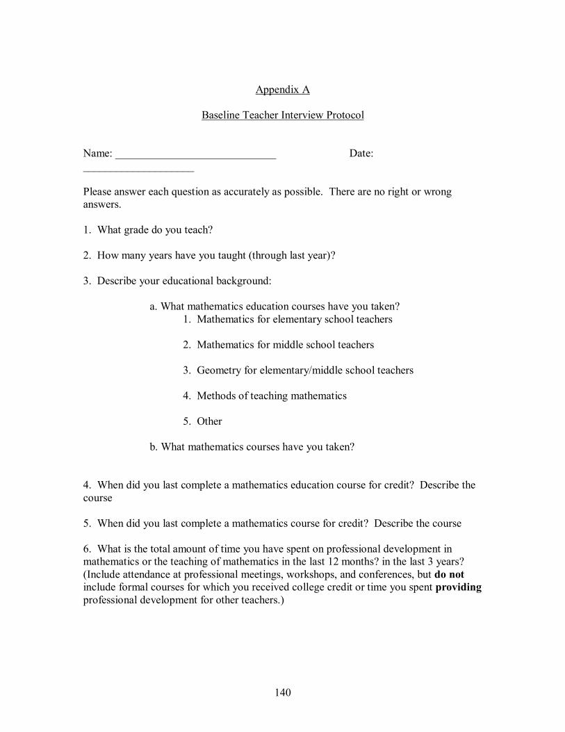
140

Appendix A

Baseline Teacher Interview Protocol Name: _____________________________ Date: ____________________ Please answer each question as accurately as possible. There are no right or wrong answers. 1. What grade do you teach? 2. How many years have you taught (through last year)? 3. Describe your educational background:

a. What mathematics education courses have you taken? 1. Mathematics for elementary school teachers 2. Mathematics for middle school teachers 3. Geometry for elementary/middle school teachers 4. Methods of teaching mathematics 5. Other

b. What mathematics courses have you taken?

4. When did you last complete a mathematics education course for credit? Describe the course 5. When did you last complete a mathematics course for credit? Describe the course 6. What is the total amount of time you have spent on professional development in mathematics or the teaching of mathematics in the last 12 months? in the last 3 years? (Include attendance at professional meetings, workshops, and conferences, but do not include formal courses for which you received college credit or time you spent providing professional development for other teachers.)

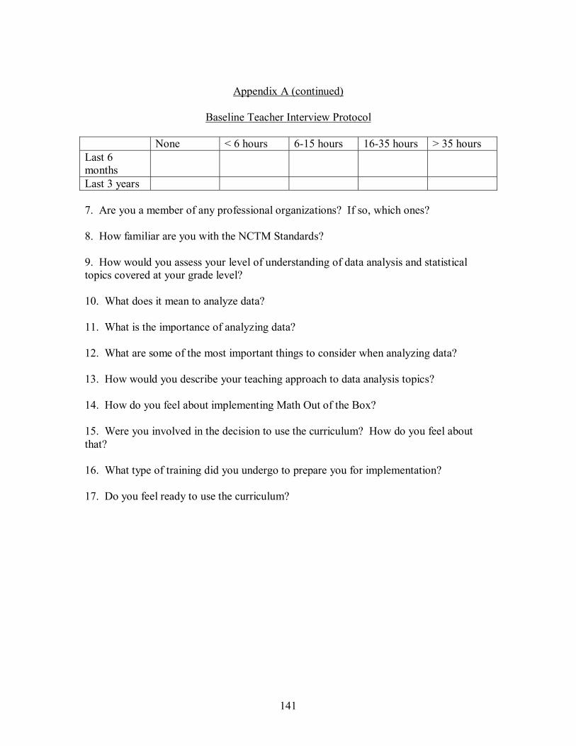
141

Appendix A (continued)

Baseline Teacher Interview Protocol None < 6 hours 6-15 hours 16-35 hours > 35 hours Last 6 months

Last 3 years 7. Are you a member of any professional organizations? If so, which ones? 8. How familiar are you with the NCTM Standards? 9. How would you assess your level of understanding of data analysis and statistical topics covered at your grade level? 10. What does it mean to analyze data? 11. What is the importance of analyzing data? 12. What are some of the most important things to consider when analyzing data? 13. How would you describe your teaching approach to data analysis topics? 14. How do you feel about implementing Math Out of the Box? 15. Were you involved in the decision to use the curriculum? How do you feel about that? 16. What type of training did you undergo to prepare you for implementation? 17. Do you feel ready to use the curriculum?

142

Appendix B

Observational Protocol

Teacher: Date: Class Length: Descriptive Notes Reflective Notes

143

Appendix C

Statistical Content Interview

Please define each concept in your own words. If you want to bring up an example that�s fine:

1. What is data?

2. What is the mean?

a. If successful to above:

i. How do you find the mean?

ii. Is there more than one way?

iii. What information does this value tell you?

3. What does the word average represent?

4. What is a median?

a. If successful to above:

i. How do you find the median?

ii. Is there more than one way?

iii. What information does this value tell you?

5. What is the difference between the median and the mean?

6. What is a mode?

a. If successful to above:

i. How do you find the mode?

ii. Is there more than one way?

iii. What information does this value tell you?

144

Appendix C (Continued)

Statistical Content Interview

7. What is the range?

a. If successful to above:

i. How do you find the range?

ii. Is there more than one way?

iii. What information does this tell you?

8. What is an outlier?

a. If successful to above:

i. How do you find an outlier?

ii. Is there more than one way?

iii. What information does this tell you?

145

Appendix D

Math Out of the Box Interview*

1. What did you learn about mathematics when teaching with Math Out of the BoxTM that you had never learned from teaching with other textbooks?

2. What did you learn about how children learn mathematics when teaching with

Math Out of the BoxTM that you had never learned from teaching with other textbooks?

3. How were the Math Out of the BoxTM lessons connected to each other? Did the

way the lessons were connected help you learn mathematics in a new way?

4. What kind of data analysis and statistical thinking did your students do with Math Out of the BoxTM? What kind did you do?

5. What was the most important thing YOU LEARNED about:

a. yourself as a teacher? b. yourself as a learner?

c. your students? d. mathematics?

*Diaz, Donna Clemson University Dissertation. 2004.

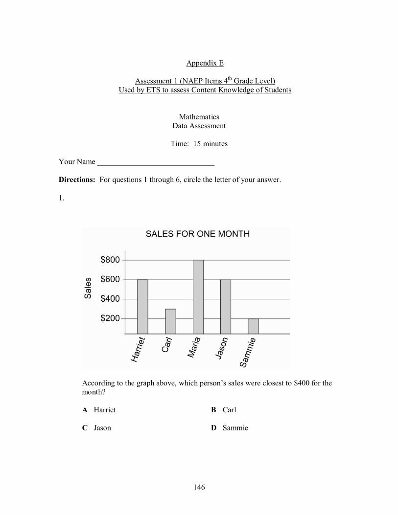
146

Appendix E

Assessment 1 (NAEP Items 4th Grade Level) Used by ETS to assess Content Knowledge of Students

Mathematics Data Assessment

Time: 15 minutes

Your Name ______________________________ Directions: For questions 1 through 6, circle the letter of your answer. 1.

According to the graph above, which person�s sales were closest to $400 for the

month? A Harriet B Carl C Jason D Sammie

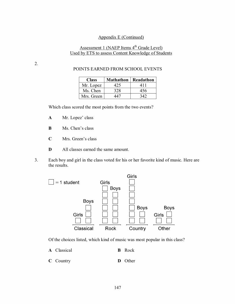
147

Appendix E (Continued)

Assessment 1 (NAEP Items 4th Grade Level) Used by ETS to assess Content Knowledge of Students

2.

POINTS EARNED FROM SCHOOL EVENTS

Class Mathathon ReadathonMr. Lopez 425 411 Ms. Chen 328 456

Mrs. Green 447 342

Which class scored the most points from the two events? A Mr. Lopez� class

B Ms. Chen�s class C Mrs. Green�s class D All classes earned the same amount.

3. Each boy and girl in the class voted for his or her favorite kind of music. Here are

the results.

Of the choices listed, which kind of music was most popular in this class?

A Classical B Rock C Country D Other

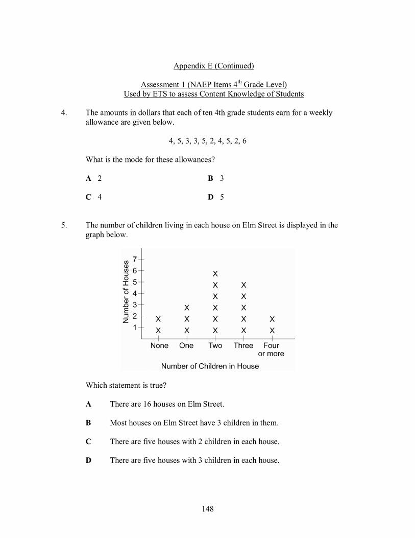
148

Appendix E (Continued)

Assessment 1 (NAEP Items 4th Grade Level) Used by ETS to assess Content Knowledge of Students

4. The amounts in dollars that each of ten 4th grade students earn for a weekly

allowance are given below.

4, 5, 3, 3, 5, 2, 4, 5, 2, 6

What is the mode for these allowances?

A 2 B 3 C 4 D 5

5. The number of children living in each house on Elm Street is displayed in the

graph below.

Which statement is true?

A There are 16 houses on Elm Street. B Most houses on Elm Street have 3 children in them.

C There are five houses with 2 children in each house.

D There are five houses with 3 children in each house.

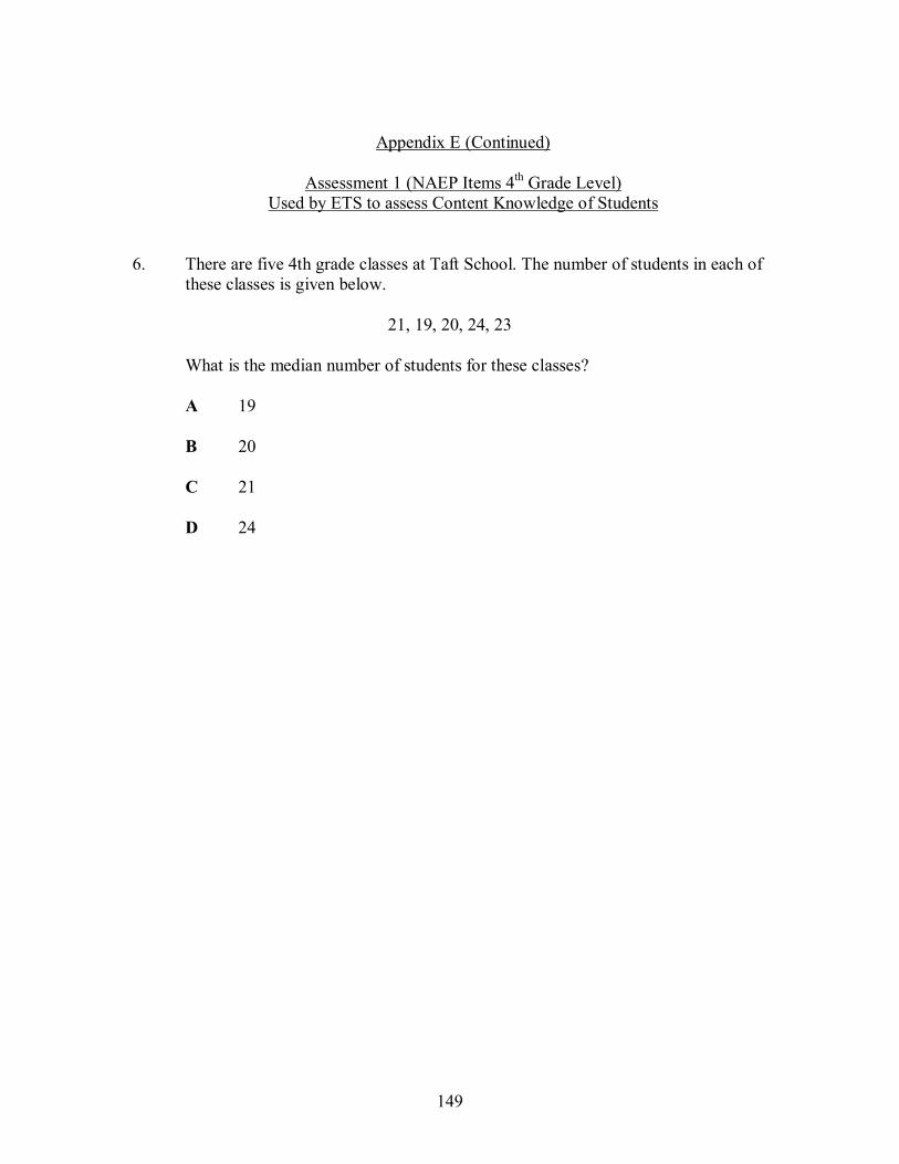
149

Appendix E (Continued)

Assessment 1 (NAEP Items 4th Grade Level) Used by ETS to assess Content Knowledge of Students

6. There are five 4th grade classes at Taft School. The number of students in each of

these classes is given below.

21, 19, 20, 24, 23

What is the median number of students for these classes? A 19 B 20 C 21 D 24

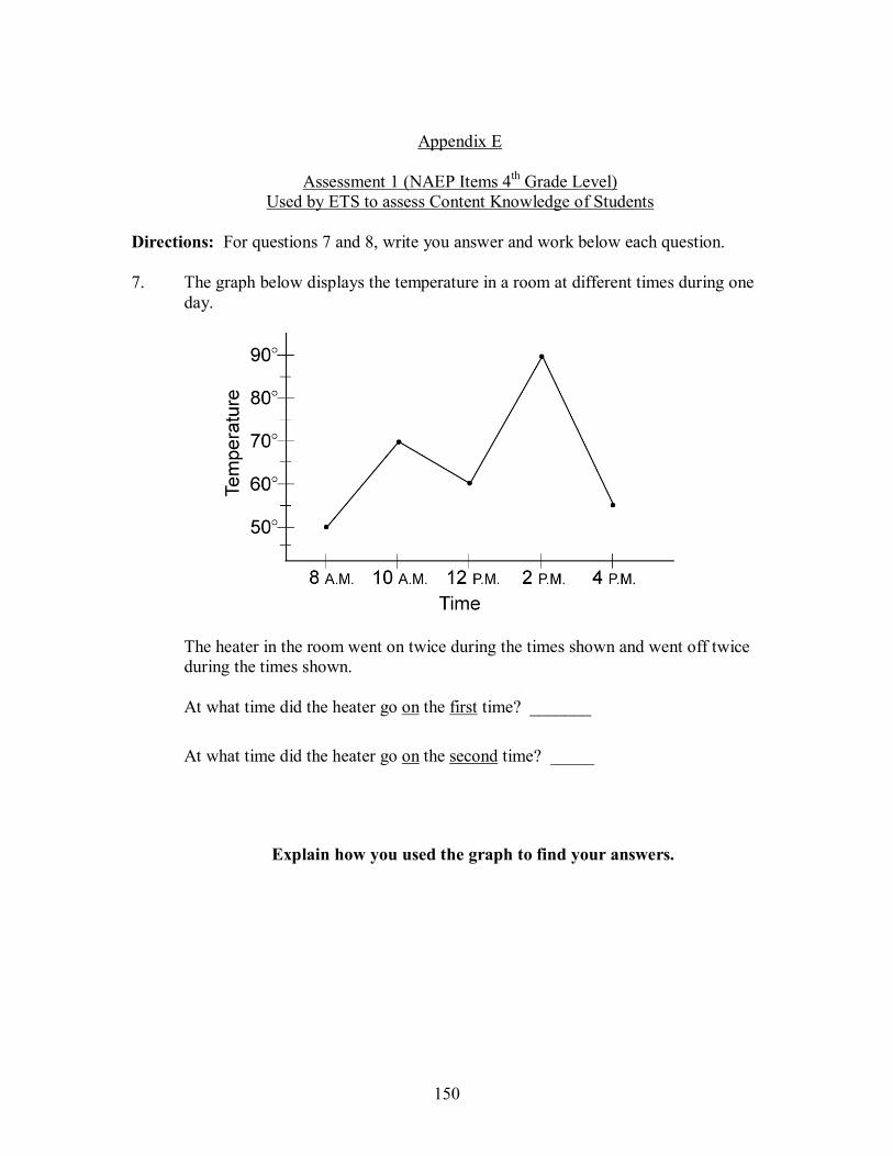
150

Appendix E

Assessment 1 (NAEP Items 4th Grade Level) Used by ETS to assess Content Knowledge of Students

Directions: For questions 7 and 8, write you answer and work below each question. 7. The graph below displays the temperature in a room at different times during one

day.

The heater in the room went on twice during the times shown and went off twice during the times shown.

At what time did the heater go on the first time? _______

At what time did the heater go on the second time? _____

Explain how you used the graph to find your answers.

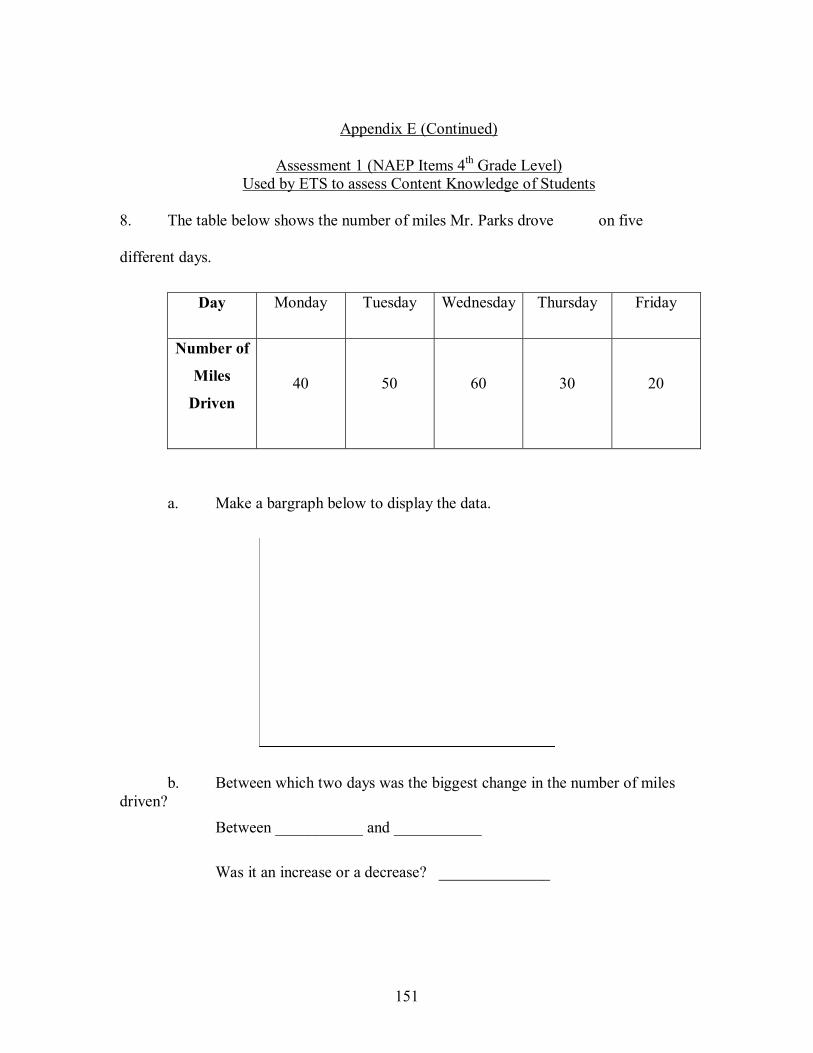
151

Appendix E (Continued)

Assessment 1 (NAEP Items 4th Grade Level) Used by ETS to assess Content Knowledge of Students

8. The table below shows the number of miles Mr. Parks drove on five

different days.

Day Monday Tuesday Wednesday Thursday Friday

Number of

Miles

Driven

40

50

60

30

20

a. Make a bargraph below to display the data.

b. Between which two days was the biggest change in the number of miles driven?

Between ___________ and ___________

Was it an increase or a decrease? ______________

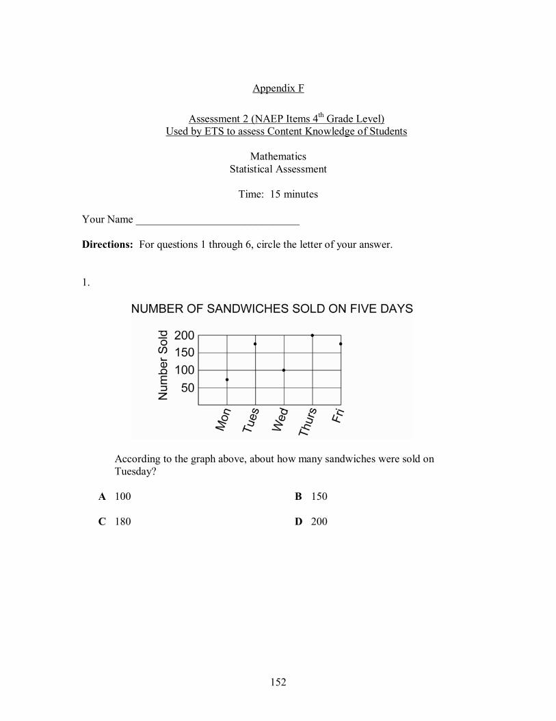
152

Appendix F

Assessment 2 (NAEP Items 4th Grade Level) Used by ETS to assess Content Knowledge of Students

Mathematics

Statistical Assessment

Time: 15 minutes Your Name ______________________________ Directions: For questions 1 through 6, circle the letter of your answer. 1.

According to the graph above, about how many sandwiches were sold on

Tuesday? A 100 B 150 C 180 D 200

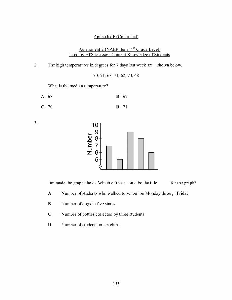
153

Appendix F (Continued)

Assessment 2 (NAEP Items 4th Grade Level) Used by ETS to assess Content Knowledge of Students

2. The high temperatures in degrees for 7 days last week are shown below.

70, 71, 68, 71, 62, 73, 68 What is the median temperature? A 68 B 69

C 70 D 71

3.

Jim made the graph above. Which of these could be the title for the graph?

A Number of students who walked to school on Monday through Friday B Number of dogs in five states C Number of bottles collected by three students D Number of students in ten clubs

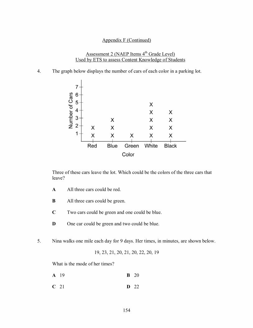
154

Appendix F (Continued)

Assessment 2 (NAEP Items 4th Grade Level) Used by ETS to assess Content Knowledge of Students

4. The graph below displays the number of cars of each color in a parking lot.

Three of these cars leave the lot. Which could be the colors of the three cars that

leave?

A All three cars could be red. B All three cars could be green. C Two cars could be green and one could be blue. D One car could be green and two could be blue.

5. Nina walks one mile each day for 9 days. Her times, in minutes, are shown below.

19, 23, 21, 20, 21, 20, 22, 20, 19

What is the mode of her times?

A 19 B 20

C 21 D 22

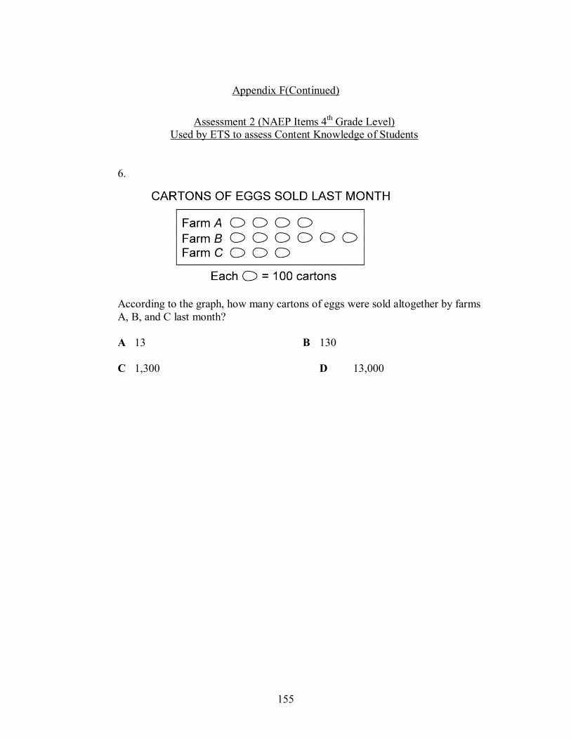
155

Appendix F(Continued)

Assessment 2 (NAEP Items 4th Grade Level) Used by ETS to assess Content Knowledge of Students

6.

According to the graph, how many cartons of eggs were sold altogether by farms

A, B, and C last month? A 13 B 130 C 1,300 D 13,000

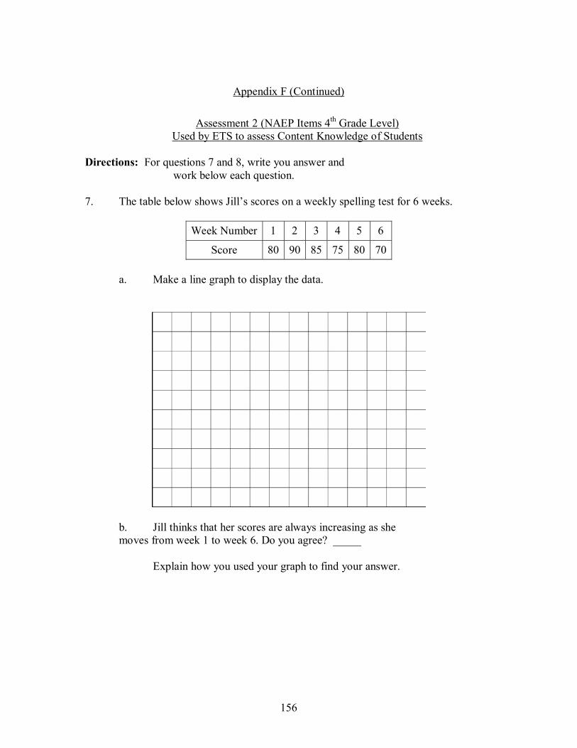
156

Appendix F (Continued)

Assessment 2 (NAEP Items 4th Grade Level) Used by ETS to assess Content Knowledge of Students

Directions: For questions 7 and 8, write you answer and work below each question. 7. The table below shows Jill�s scores on a weekly spelling test for 6 weeks.

Week Number 1 2 3 4 5 6

Score 80 90 85 75 80 70

a. Make a line graph to display the data.

b. Jill thinks that her scores are always increasing as she moves from week 1 to week 6. Do you agree? _____ Explain how you used your graph to find your answer.

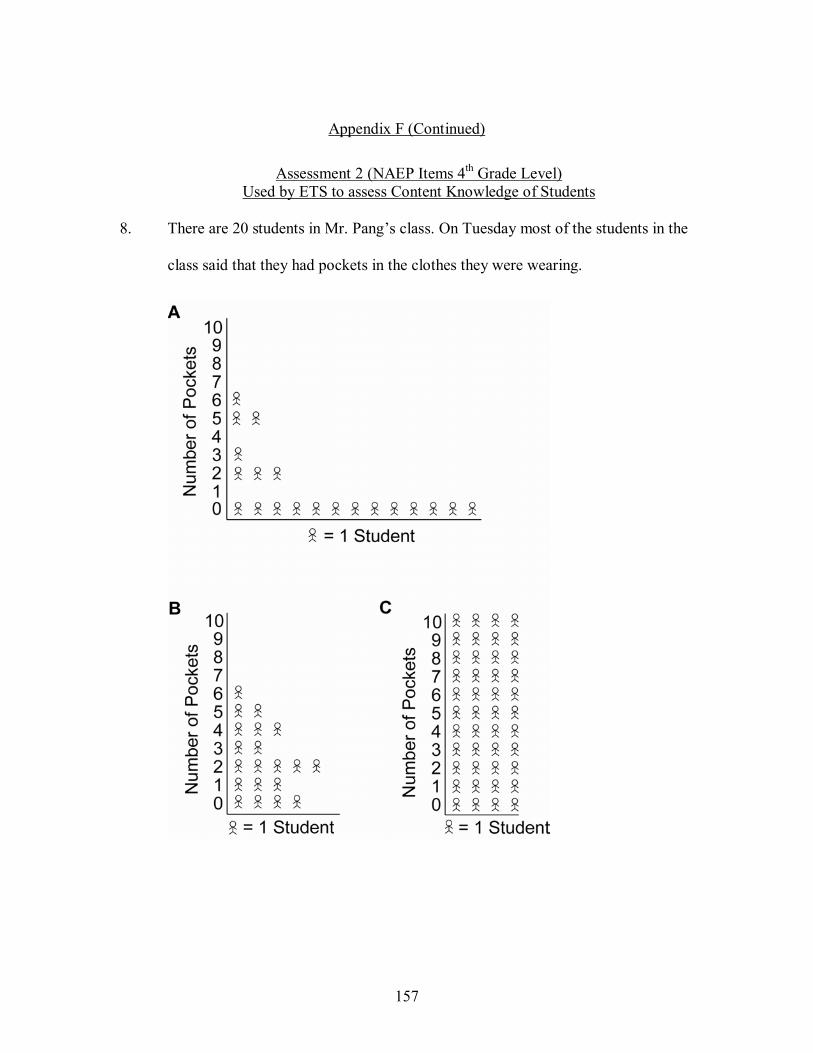
157

Appendix F (Continued)

Assessment 2 (NAEP Items 4th Grade Level) Used by ETS to assess Content Knowledge of Students

8. There are 20 students in Mr. Pang�s class. On Tuesday most of the students in the

class said that they had pockets in the clothes they were wearing.

158

Appendix F (Continued)

Assessment 2 (NAEP Items 4th Grade Level) Used by ETS to assess Content Knowledge of Students

Which of the graphs (A, B, or C) most likely shows the number of pockets that each child

had? __________

Explain why you chose that graph.

Explain why you did not choose the other graphs.

This is the end. If you finish early, please check your work.

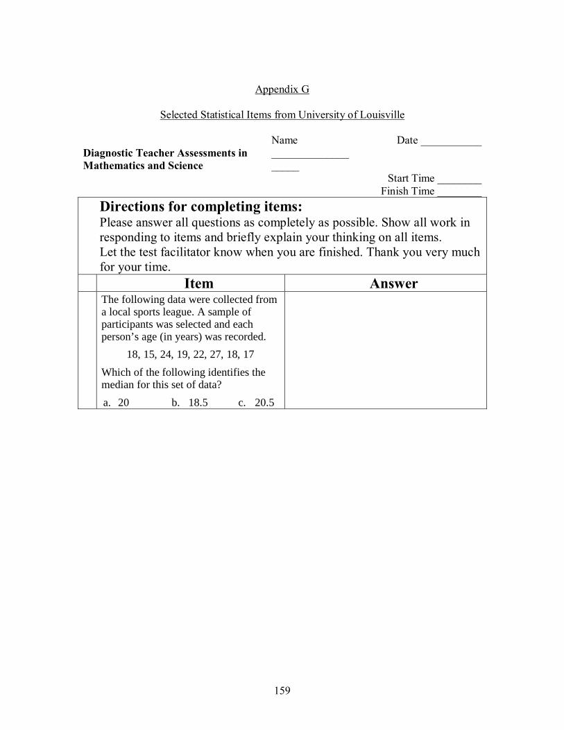
159

Appendix G

Selected Statistical Items from University of Louisville

Name ___________________

Date ___________Diagnostic Teacher Assessments in Mathematics and Science Start Time ________

Finish Time ________Directions for completing items: Please answer all questions as completely as possible. Show all work in responding to items and briefly explain your thinking on all items. Let the test facilitator know when you are finished. Thank you very much for your time.

Item Answer The following data were collected from a local sports league. A sample of participants was selected and each person’s age (in years) was recorded.

18, 15, 24, 19, 22, 27, 18, 17

Which of the following identifies the median for this set of data?

a. 20 b. 18.5 c. 20.5

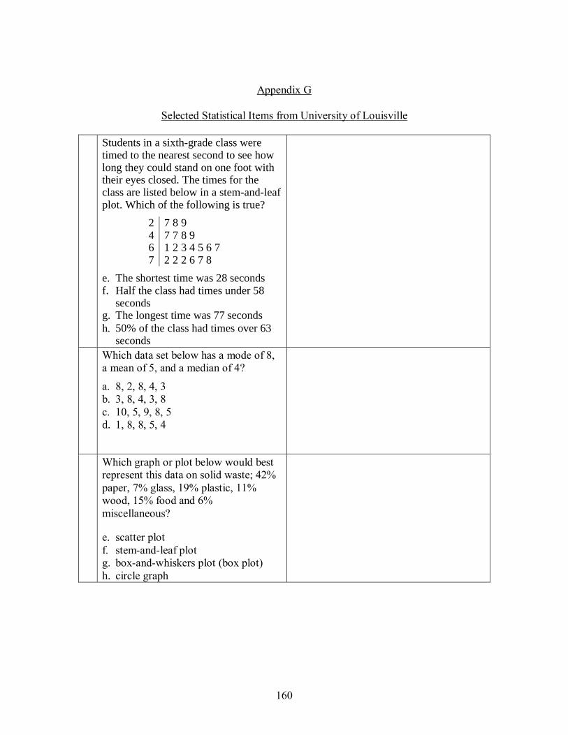
160

Appendix G

Selected Statistical Items from University of Louisville

Students in a sixth-grade class were timed to the nearest second to see how long they could stand on one foot with their eyes closed. The times for the class are listed below in a stem-and-leaf plot. Which of the following is true?

2 7 8 9 4 7 7 8 9 6 1 2 3 4 5 6 7 7 2 2 2 6 7 8

e. The shortest time was 28 seconds f. Half the class had times under 58

seconds g. The longest time was 77 seconds h. 50% of the class had times over 63

seconds

Which data set below has a mode of 8, a mean of 5, and a median of 4?

a. 8, 2, 8, 4, 3 b. 3, 8, 4, 3, 8 c. 10, 5, 9, 8, 5 d. 1, 8, 8, 5, 4

Which graph or plot below would best represent this data on solid waste; 42% paper, 7% glass, 19% plastic, 11% wood, 15% food and 6% miscellaneous?

e. scatter plot f. stem-and-leaf plot g. box-and-whiskers plot (box plot) h. circle graph

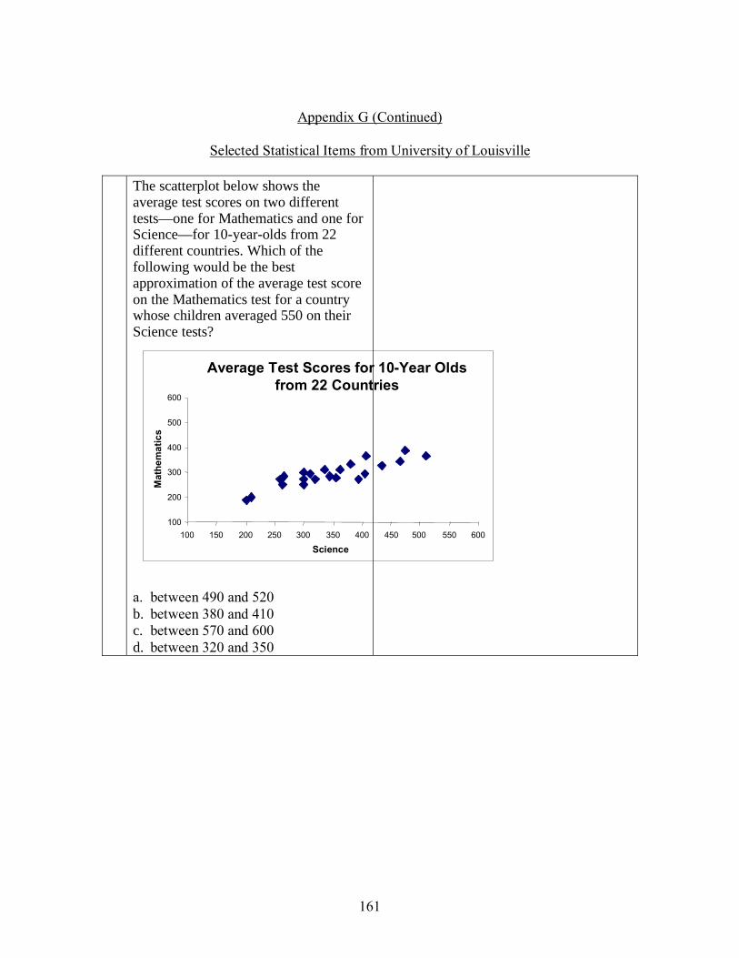
161

Appendix G (Continued)

Selected Statistical Items from University of Louisville

The scatterplot below shows the average test scores on two different tests—one for Mathematics and one for Science—for 10-year-olds from 22 different countries. Which of the following would be the best approximation of the average test score on the Mathematics test for a country whose children averaged 550 on their Science tests?

a. between 490 and 520 b. between 380 and 410 c. between 570 and 600 d. between 320 and 350

Average Test Scores for 10-Year Oldsfrom 22 Countries

100 200 300 400 500 600

100 150 200 250 300 350 400 450 500 550 600

Science

Mat

hem

atic

s

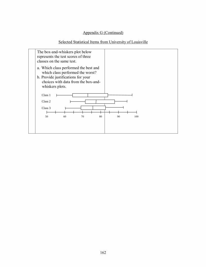
162

Appendix G (Continued)

Selected Statistical Items from University of Louisville

The box-and-whiskers plot below represents the test scores of three classes on the same test. a. Which class performed the best and

which class performed the worst? b. Provide justifications for your

choices with data from the box-and-whiskers plots.

50

Class 1 Class 2 Class 3

60 70 80 90 100

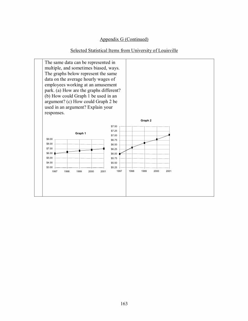
163

Appendix G (Continued)

Selected Statistical Items from University of Louisville

The same data can be represented in multiple, and sometimes biased, ways. The graphs below represent the same data on the average hourly wages of employees working at an amusement park. (a) How are the graphs different? (b) How could Graph 1 be used in an argument? (c) How could Graph 2 be used in an argument? Explain your responses.

Graph 1

$3.00 $4.00 $5.00 $6.00 $7.00 $8.00 $9.00

1997 1998 1999 2000 2001

Graph 2

$5.25

$5.50

$5.75

$6.00

$6.25

$6.50

$6.75

$7.00

$7.25

$7.50

1997 1998 1999 2000 2001

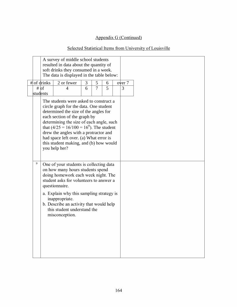
164

Appendix G (Continued)

Selected Statistical Items from University of Louisville

A survey of middle school students resulted in data about the quantity of soft drinks they consumed in a week. The data is displayed in the table below:

# of drinks 2 or fewer 3 5 6 over 7 # of

students 4 6 7 5 3

The students were asked to construct a circle graph for the data. One student determined the size of the angles for each section of the graph by determining the size of each angle, such that (4/25 = 16/100 = 160). The student drew the angles with a protractor and had space left over. (a) What error is this student making, and (b) how would you help her?

9 One of your students is collecting data on how many hours students spend doing homework each week night. The student asks for volunteers to answer a questionnaire. a. Explain why this sampling strategy is

inappropriate. b. Describe an activity that would help

this student understand the misconception.

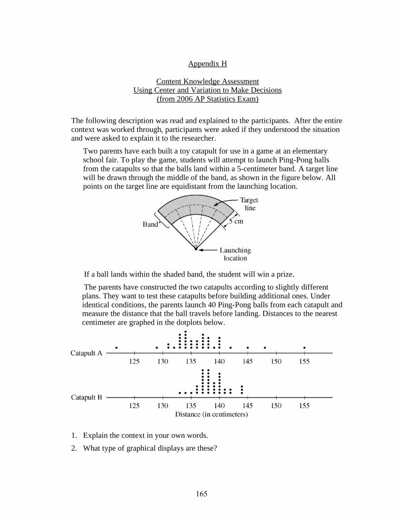
165

Appendix H

Content Knowledge Assessment Using Center and Variation to Make Decisions

(from 2006 AP Statistics Exam)

The following description was read and explained to the participants. After the entire context was worked through, participants were asked if they understood the situation and were asked to explain it to the researcher.

Two parents have each built a toy catapult for use in a game at an elementary school fair. To play the game, students will attempt to launch Ping-Pong balls from the catapults so that the balls land within a 5-centimeter band. A target line will be drawn through the middle of the band, as shown in the figure below. All points on the target line are equidistant from the launching location.

If a ball lands within the shaded band, the student will win a prize.

The parents have constructed the two catapults according to slightly different plans. They want to test these catapults before building additional ones. Under identical conditions, the parents launch 40 Ping-Pong balls from each catapult and measure the distance that the ball travels before landing. Distances to the nearest centimeter are graphed in the dotplots below.

1. Explain the context in your own words.

2. What type of graphical displays are these?

166

Appendix H (Continued)

Content Knowledge Assessment Using Center and Variation to Make Decisions (from 2006 AP Statistics Exam)

3. What information can you find based on what is presented (i.e. mean, median, mode, range, and standard deviation)?

4. If the parents want to maximize the probability of having the Ping-Pong balls land within the band, which one of the two catapults, A or B, would be better to use than the other? Catapult A or B can be placed anywhere parents desire to maximize their chances of landing balls within the 5 cm band. Justify your choice.

5. Using the catapult that you chose in question 4, how many centimeters from the target line should this catapult be placed? Explain why you chose this distance.

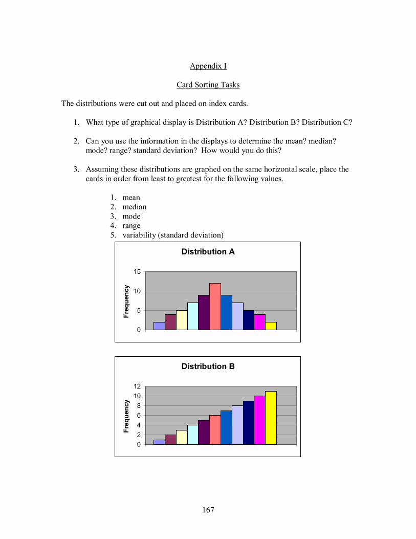
167

Appendix I

Card Sorting Tasks The distributions were cut out and placed on index cards.

1. What type of graphical display is Distribution A? Distribution B? Distribution C?

2. Can you use the information in the displays to determine the mean? median? mode? range? standard deviation? How would you do this?

3. Assuming these distributions are graphed on the same horizontal scale, place the

cards in order from least to greatest for the following values.

1. mean 2. median 3. mode 4. range 5. variability (standard deviation)

Distribution A

0

5

10

15

Freq

uenc

y

Distribution B

02468

1012

Freq

uenc

y

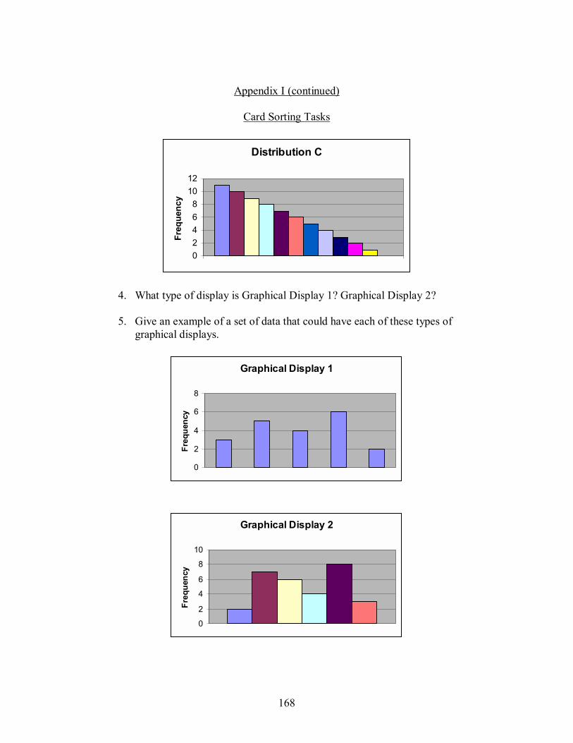
168

Appendix I (continued)

Card Sorting Tasks

Distribution C

02468

1012

Freq

uenc

y

4. What type of display is Graphical Display 1? Graphical Display 2? 5. Give an example of a set of data that could have each of these types of

graphical displays.

Graphical Display 1

0

2

4

6

8

Freq

uenc

y

Graphical Display 2

0

2

4

6

8

10

Freq

uenc

y

169

REFERENCES

Ball, D.L. (1988). Unlearning to teach mathematics (Issue Paper 88-1). East Lansing: Michigan State University, National Center for Research on Teacher Education.

Ball, D.L. (1989). Research on teaching mathematics: Making subject matter

knowledge part of the equation. In J. Brophy (Ed.), Advances in research on teaching: Vol. 2. Teachers� subject matter knowledge and classroom instruction. (pp. 1-48). Greenwich: JAI.

Ball, D.L. (1990). Prospective elementary and secondary teachers� understanding

of division. Journal for Research in Mathematics Education, 21(2), 132-144.

Ball, D.L. (1990). The mathematical understandings that pre-service teachers

bring to teacher education. Elementary School Journal, 90, 449-466. Ball, D.L. (1991). Research on teaching mathematics: Making subject matter

knowledge part of the equation. In J. E. Brophy (Ed.), Advances in research on teaching: Teachers� subject matter knowledge and classroom instruction (Vol. 2, pp. 1-48). Greenwich, CT: JAI Press.

Ball, D., Hill, H., & Bass, H. (2005). Knowing mathematics for teaching: Who

knows mathematics well enough to teach third grade, and how can we decide? American Educator, 14-22, 43-46.

Begg, A., & Edwards, R. (1999). Teachers' ideas about teaching statistics. Paper

presented at the joint conference of the AARE and NZARE, Melbourne. Borko, H., Eisenhar, M., Brown, C., Underhill, R., Jones, D., & Agard, P. (1992).

Learning to teach hard mathematics: Do novice teachers and their instructors give up too easily? Journal for Research in Mathematics, 23(3), 194-222.

Bush, W. et.al. (under review). Diagnostic mathematics assessment for middle

school teachers. Journal of Mathematics Teacher Education. Campbell, P. F. & White, D. Y. (1997). Project IMPACT: Influencing and

supporting teacher change in predominantly minority schools. In E. Fennema & B. S. Nelson (Eds.) Mathematics Teachers in Transition (pp. 309-355). Mahwah, NJ: Erlbaum.

170

Clarke, B. (1995). Expecting the unexpected: Critical incidents in the mathematics classroom. Unpublished doctoral dissertation, University of Wisconsin�Madison.

Cobb, G., and Moore, D. S. (1997), Mathematics, Statistics and Teaching. The

American Mathematical Monthly, 104(11), 801-823. Cobb, P. (1999). Individual and collective mathematical development: The case

of statistical data analysis. Mathematical Thinking and Learning, 1(1), 5-43.

Cobb, P., Bauersfeld, H. (Eds.) (1995). The Emergence of Mathematical

Meaning: Interacting in Classroom Cultures (Studies in Mathematical Thinking and Learning). Hillsdale, NJ: Lawrence Erlbaum.

Collopy, R. (2003). Curriculum materials as a professional development tool: how

a mathematics textbook affected two teachers� learning. The Elementary School Journal, 103(3), 287-311.

Cooney, T. J. (1994). Teacher education as an exercise in adaptation. In D.B.

Aichele & A.F. Coxford (Eds.) Professional Development for Teachers of Mathematics, pp. 9-22. Reston, VA: NCTM.

Cresswell, J.W. (1998). Qualitative Inquiry and Research Design: Choosing

Among Five Traditions. London: Sage Publications. Dewey, J. (1997). How We Think. New York: Dover Publications. Diaz, D. P. (2004). The role of standards-based curricula in teacher learning and

instructional reform. Unpublished doctoral dissertation. Clemson University.

Doerr, H. & English, L. (2003). A modeling perspective on students�

mathematical reasoning about data. Journal for research in mathematics education, 34(2), 110-136.

Enochs, L., & Gabel, D. (1984). Preservice elementary teachers� conceptions of

volume. School Science and Mathematics, 84(8), 670-680. Fennema, E. & Franke, M.L. (1992). Teachers� knowledge and its impact. In D.

Grouws (Ed.) Handbook of research on mathematics teaching and learning (pp.147-163). New York: MacMillan.

171

Fischbein, E., Nello, M., & Marino, M. (1991). Factors affecting probabilistic judgments in children and adolescents. Educational Studies in Mathematics, 22, 523-549.

Fischbein, E. & Schnarch, D. (1997). The evolution with age of probabilistic,

intuitively based misconceptions. Journal for Research in Mathematics Education, 28, 96-105.

Franklin, C. et.al. (2005). A curriculum framework for preK-12 statistics

education. Paper presented to the American Statistical Association Board of Directors for Endorsement.

Gal, I., Rothschild, K., & Wagner, D.A. (1990). Statistical concepts and

statistical reasoning in school children: Convergence or divergence. Paper presented at the annual meeting of the American Educational Research Association, Boston, MA.

Garfield, J. (1988). Obstacles to effective teaching of probability and statistics.

Paper presented at the Research Presession of the National Council of Teachers of Mathematics 66th Annual Meeting, Chicago.

Garfield, J. & Ahlgren, A. (1994). Student reactions to learning about probability and statistics: evaluating the quantitative literacy project. School science and mathematics, 94(2), pp. 84-95.

Graeber, A., Tirosh, D., & Glover, R. (1989). Preservice teachers� misconceptions

in solving verbal problems in multiplication and division. Journal for Research in Mathematics Education, 20(1), 95-102.

Greer, B. & Ritson, R. (1994). Readiness of teachers in Northern Ireland to teach

Data Handling. Proceedings of the Fourth International Conference on Teaching Statistics, Vol. 1. Marrakech, Morocco. National Organising Committee of the Fourth International Conference on Teaching Statistics, pp. 49-56.

Hatano, G. (1982). Cognitive consequences of practice in culture-specific

procedural skills. Quarterly Newsletter of the Laboratory of Comparative Human Cognition, 4(1), 15-18.

Hiebert, J., & Lefevre, P. (1986). Conceptual and procedural knowledge in

mathematics: An introductory analysis. In J. Hiebert and P. Lefevre (Eds.), Conceptual and procedural knowledge: The case of mathematics, pp. 1-27. Hillsdale, NJ: Lawrence Erlbaum.

172

Horton, R. (1997). Mathematics teachers� knowledge of and attitudes toward stochastics and the effects of a stochastics in-service program. Unpublished doctoral dissertation, University of Cincinnati, OH.

Jones, G. et. al. (1999). Students� probabilistic thinking in instruction. Journal for

Research in Mathematics Education, 30, 487-519. Konold, C. & Higgins, T. (2003). Reasoning about data. In J. Kilpatrick, W.G.

Martin, & D.E. Schifter (Eds.), A research companion to principles and standards for school mathematics. Reston, VA: NCTM.

Konold, C. & Khalil, K. (2003). If U can graff these numbers�2,15,6�your stat

literate. Paper presented at the annual meeting of the American Educational Research Association, Chicago, IL.

Konold, C., & Pollatsek, A. (2002). Data analysis as the search for signals in

noisy processes. Journal for Research in Mathematics Education, 33(4), 259-289.

Konold, C., Robinson, A., Khalil, K., Pollatsek, A., Well, A., Wing, R., & Mayr,

S. (2002). Students� use of modal clumps to summarize data. Paper presented at the Sixth International Conference on Teaching Statistics, Cape Town, South Africa.

Lehrer, R., & Franke, M.L. (1992). Applying personal construct psychology to the

study of teachers� knowledge of fractions. Journal for Research in Mathematics Education, 23(3), 223-241.

Lincoln, Y., & Guba, E. (1985). Naturalistic inquiry. Newbury Park, CA: Sage

Publications. McGatha, M., Cobb, P., McClain, K. (1998). An analysis of students� statistical

understandings. Paper presented at the Annual Meeting of the American Educational Research Association, San Diego, CA.

McGatha, M., Cobb, P., & McClain, K. (2002). An analysis of students� initial

statistical understandings: Developing a conjectured learning trajectory. Journal of Mathematical Behavior, 16, 339-355.

Menon, R. (1998). Preservice teachers� understanding of perimeter and area.

School Science and Mathematics, 98(7), 361-68. Mevarech, Z. (1983). A deep structure model of students� statistical

misconceptions. Educational studies in mathematics, 14, 415-429.

173

Mokros, J., & Russell, S. J. (1995). Children�s concepts of average and representativeness. Journal for Research in Mathematics Education, 26, 20-39.

Moss, D., et al. (2005). Developing Algebraic Thinking: Plotting and Growing,

Teacher�s Manual, Third Grade, Burlington, NC: Carolina Biological Supply.

Moss, D., et al. (2005). Developing Algebraic Thinking: Plotting and Growing,

Teacher�s Manual, Fourth Grade, Burlington, NC: Carolina Biological Supply.

National Council of Teachers of Mathematics. (1989). Curriculum and evaluation

standards for school mathematics. Reston, VA: NCTM. National Council of Teachers of Mathematics. (1991). Professional standards for

teaching mathematics. Reston, VA: NCTM. National Council of Teachers of Mathematics. (2000). Principles and standards

for school mathematics. Reston, VA: NCTM. Noss, R., Pozzi, S., & Hoyles, C. (1999). Touching epistemologies: Meanings of

average and variation in nursing practice. Educational Studies in Mathematics, 40, 25-51.

Reinke, K. (1997). Area and perimeter: Preservice teachers� confusion. School

Science and Mathematics, 97(2), 75-77. Remillard, J. (2000). Can curriculum materials support teachers� learning? Two

fourth-grade teachers� use of a new mathematics text. The Elementary School Journal, 100(4), 331-350.

Richardson, V., and Placier, P. (2001). Teacher change. In V. Richardson (Ed.)

Handbook of Research on Teaching, 4th ed., pp. 905-947. Washington, DC: AERA.

Ryle, G. (1949). The Concept of Mind. Chicago, IL: University of Chicago Press. Scheffler, I. (1965). Conditions of knowledge: An introduction to epistemology

and education. Glenview, IL: Scott, Foresman, and Company. Scheaffer, R. (1986). The quantitative literacy project. Teaching Statistics, 8(2),

pp. 34-38.

174

Scheaffer, R. (1991). The ASA-NCTM Quantitative Literacy Program: An overview. In D. Vere-Jones (Ed.), Proceedings of the Third International Conference on Teaching Statistics (pp. 45-49). Voorburg, The Netherlands: International Statistical Institute Publications.

Scheaffer, R. (2001). Statistics education: perusing the past, embracing the

present, and charting the future. Newsletter for the section on statistical education. 7(1). American Statistical Association.

Schon, D. (1983). The Reflective Practitioner. New York: Basic Books. Shaughnessy, J.M. (1985). Rote versus conceptual emphases in teaching

elementary probability. Journal for research in mathematics education, 18(5), 364-374.

Shaughnessy, J.M. (1992). Research in probability and statistics: reflections and

directions. In D. Grouws (Ed.) Handbook of Research on Mathematics Teaching and Learning (pp.465-493). New York: MacMillan.

Shaughnessy, J.M. (1993). Probability and statistics. Mathematics Teacher, 86(3),

244-248. Shaughnessy, J. M., & Zawojewski, J. S. (1999). Secondary students�

performance on data and chance in the 1996 NAEP. Mathematics Teacher, 92, 713�718.

Shulman, L. (1987). Knowledge and teaching: Foundations of the new reform.

Harvard Educational Review, 57(1), 1-22. Simon, M. (1993). Prospective elementary teachers� knowledge of division.

Journal for Research in Mathematics Education, 24(3), 233-253. Simon, M., & Blume, G. (1994). Building an understanding of multiplicative

relationships: A study of prospective elementary teachers. Journal for Research in Mathematics Education, 25(5), 472-494.

Skemp, R. (1978). Relational understanding and instrumental understanding.

Arithmetic teacher, 26(3), 9-15. Star, J.R. (2000). On the relationship between knowing and doing in procedural

learning. In B. Fishman & S. O'Connor-Divelbiss (Eds.), Proceedings of fourth international conference of the Learning Sciences (pp. 80-86). Mahwah, NJ: Lawrence Erlbaum.

175

Star, J.R. (2005). Reconceptualizing procedural knowledge. Journal for Research in Mathematics Education, 36(5), 404-411.

Thipkong, S., & Davis, E. (1991). Preservice elementary teachers�

misconceptions in interpreting and applying decimals. School Science and Mathematics, 91(3), 93-99.

Thompson, A.G. (1991). The development of teachers� conceptions of

mathematics teaching. In R. G. Underhill (Ed.), Proceedings of the thirteenth annual meeting of the North American Chapter of the International Group for the Psychology of Mathematics Education. (Vol.2; pp. 8-14). Blacksburgh, VA: Virginia Polytechnic Institute.

Tirosh, D., & Graeber, A. (1990). Inconsistencies in preservice elementary

teachers� beliefs about multiplication and division. Focus on Learning Problems in Mathematics, 12 (3-4), 65-74.

Watson, J., Kelly, B.A., Callingham, R.A., Shaughnessy, J.M. (2003). The

measurement of school students� understanding of statistical variation. International Journal of Mathematics Education Science & Technology, 34(1), 1-29.

Watson, J.M., & Moritz, J.B. (1999). The beginning of statistical inference:

Comparing two sets of data. Educational Studies in Mathematics, 37, 145-168.

Wheeler, M., & Feghali, I. (1983). Much ado about nothing. Journal for Research

in Mathematics Education, 14(3), 147-155. Zazkis, R., & Campbell, S. (1996). Divisibility and multiplicative structure of

natural numbers; Preservice teachers� understanding. Journal for Research in Mathematics Education, 27(5), 540-563.

Zawojewski, J.S. & Heckman, D.J. (1997). What do students know about data

analysis, statistics, and probability? In P.A. Kenney & E.A. Silver (Eds.), Results from the sixth mathematics assessment of the National Assessment of Educational Progress (pp. 195-223). Reston, VA: National Council of Teachers of Mathematics.

Zawojewski, J.S. & Shaughnessy, J.M. (1999). Data and chance. In P.A. Kenney

& E.A. Silver (Eds.), Results from the seventh mathematics assessment of the National Assessment of Educational Progress (pp.235-268). Reston, VA: National Council of Teachers of Mathematics.

176

Zawojewski, J.S. & Shaughnessy, J.M. (2000). Mean and median: Are they really so easy. Mathematics Teaching in the Middle School. 5(7), pp.436-440.