Embed Size (px)
Citation preview
Elementary Partial Differential Equations∗
William V. Smith
Introduction.
Partial differential equations (PDEs) is one of the oldest subjects in math-
ematical analysis. Its development extends back to Euler’s work in the 1700s,
together with Brooks Taylor and others.
Problems arising in the study of PDEs have motivated many of the prin-
ciple developments in classical and modern analysis. For example, harmonic
analysis (Fourier), complex analysis (Cauchy, Riemann), theory of integral
equations (Fredholm, Hilbert), Hilbert and Banach space theory, fixed point
theorems (Schauder), theory of distributions (L. Schwartz) and many others.
At present the theory of PDEs is one of the most active fields of research
in modern mathematics. Each month Mathematical Reviews contains many
pages of reviews of publications on PDE’s. As another example Professor
C. Miranda published a monograph on “PDEs of Elliptic Type” in 1954. It
contained a bibliography of more than 600 research papers published between
1924-1953. In the revised edition published in 1968, Miranda estimated that
∗Copyright c©2011, William V. Smith. All rights reserved.
1
to bring the bibliography up to date more than 1600 items would have to be
added. The process has continued to accelerate.
At the present time, it is impossible to present in a single course a com-
plete survey of what is known as PDEs and the properties of their solutions.
Many advanced monographs exist and in many cases their contents scarcely
overlap.
Plan for this course
A study of classical theories for some of the simplest PDEs. We shall
use as a source, V. Smirnov, A Course in Higher Mathematics, vols. II and
IV, and C. H. Wilcox, “Notes on PDEs.”1 The modern functional analytic
theories of PDEs must wait for further courses.
Contents
Chapter 1. Heat Conduction in a Slab. ————————————–p. 3
Chapter 2. Wave Propagation on a Taut String. ————————– p. 13
Chapter 3. Steady Temperature in a Circular Cylinder. —————- p. 32
Chapter 4. Basic Concepts in the Theory of Heat Conduction. —— p. 48
Chapter 5. The Cauchy Problem for the Heat Equation in 1 Space Dimen-
sion. — p. 77
Chapter 6. Steady Temperature in a Finite Cylinder. Vibration of a Drum
Head— p. 98
Appendices: Classification of PDEs. Bessel functions and Sturm-Lioville
problems. Fourier series. p. 117-143.
1Used by permission.
2
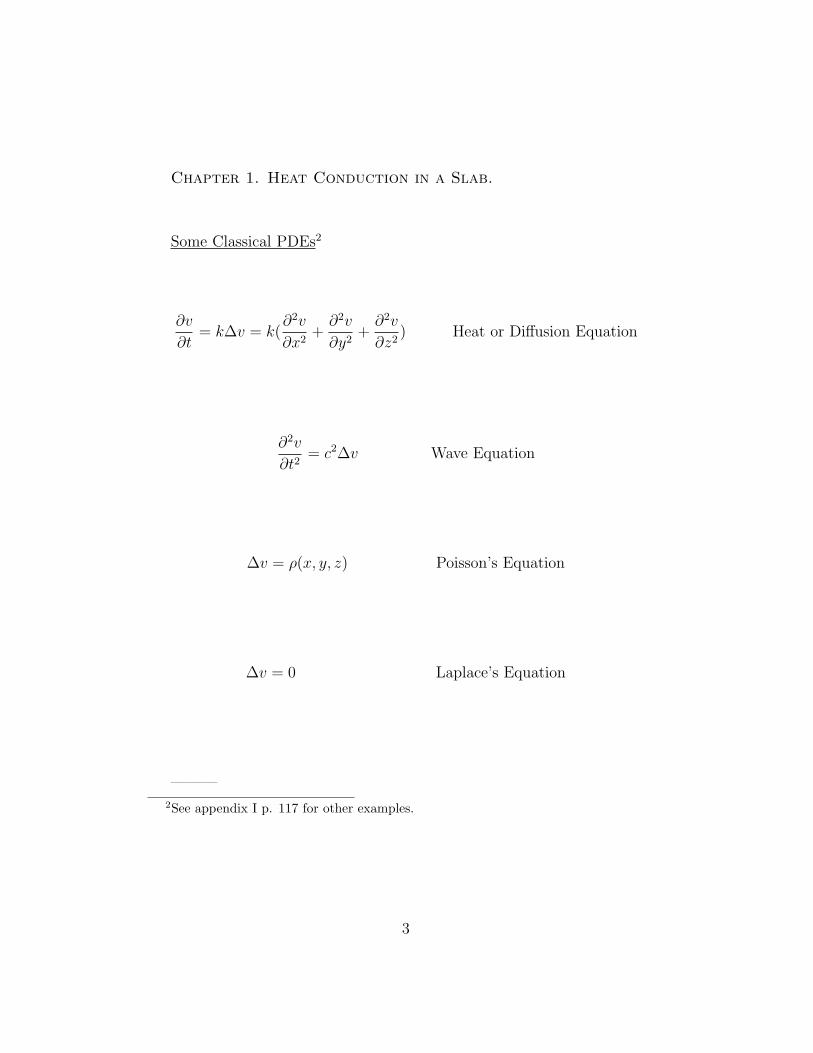
Chapter 1. Heat Conduction in a Slab.
Some Classical PDEs2
∂v
∂t= k∆v = k(
∂2v
∂x2+∂2v
∂y2+∂2v
∂z2) Heat or Diffusion Equation
∂2v
∂t2= c2∆v Wave Equation
∆v = ρ(x, y, z) Poisson’s Equation
∆v = 0 Laplace’s Equation
———
2See appendix I p. 117 for other examples.
3
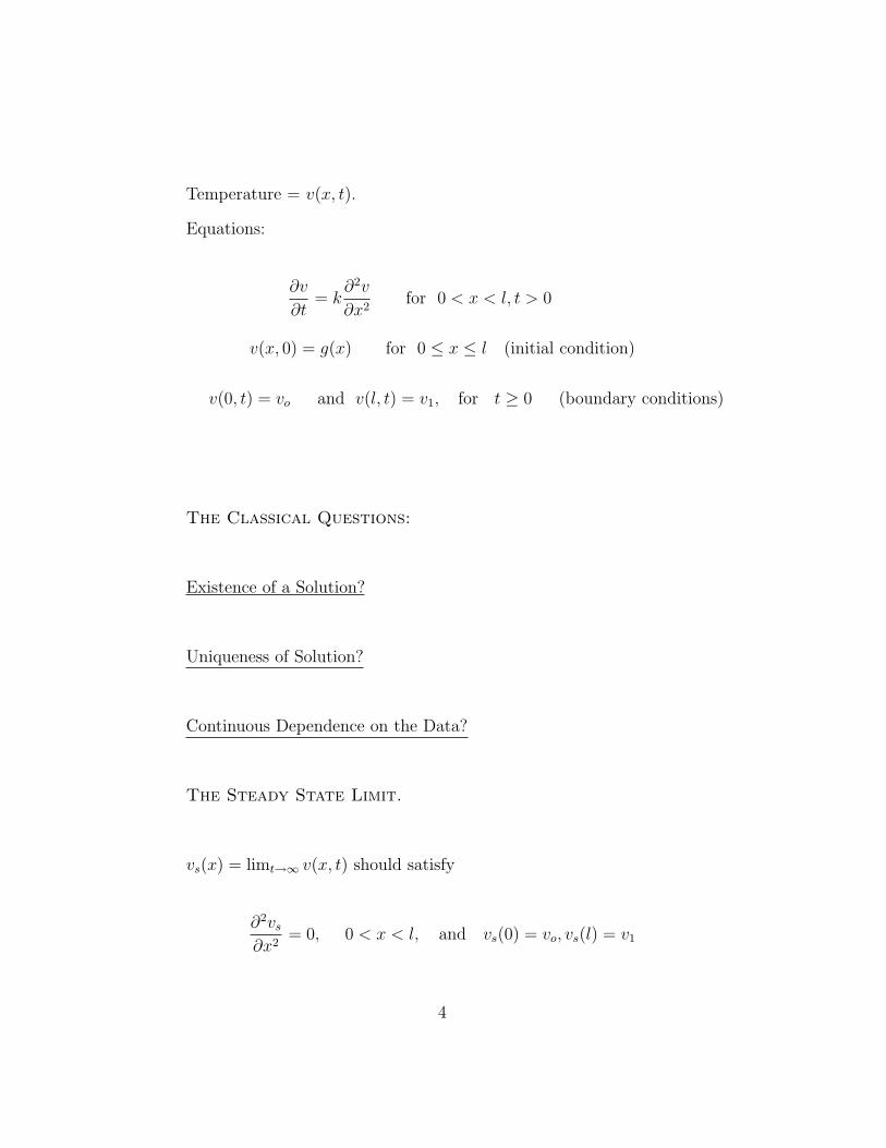
Temperature = v(x, t).
Equations:
∂v
∂t= k
∂2v
∂x2for 0 < x < l, t > 0
v(x, 0) = g(x) for 0 ≤ x ≤ l (initial condition)
v(0, t) = vo and v(l, t) = v1, for t ≥ 0 (boundary conditions)
The Classical Questions:
Existence of a Solution?
Uniqueness of Solution?
Continuous Dependence on the Data?
The Steady State Limit.
vs(x) = limt→∞ v(x, t) should satisfy
∂2vs∂x2
= 0, 0 < x < l, and vs(0) = vo, vs(l) = v1
4
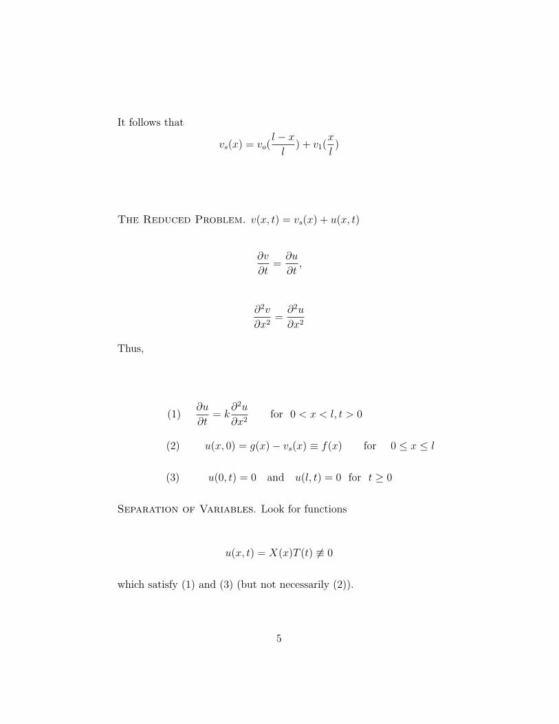
It follows that
vs(x) = vo(l − xl
) + v1(x
l)
The Reduced Problem. v(x, t) = vs(x) + u(x, t)
∂v
∂t=∂u
∂t,
∂2v
∂x2=∂2u
∂x2
Thus,
(1)∂u
∂t= k
∂2u
∂x2for 0 < x < l, t > 0
(2) u(x, 0) = g(x)− vs(x) ≡ f(x) for 0 ≤ x ≤ l
(3) u(0, t) = 0 and u(l, t) = 0 for t ≥ 0
Separation of Variables. Look for functions
u(x, t) = X(x)T (t) 6≡ 0
which satisfy (1) and (3) (but not necessarily (2)).
5
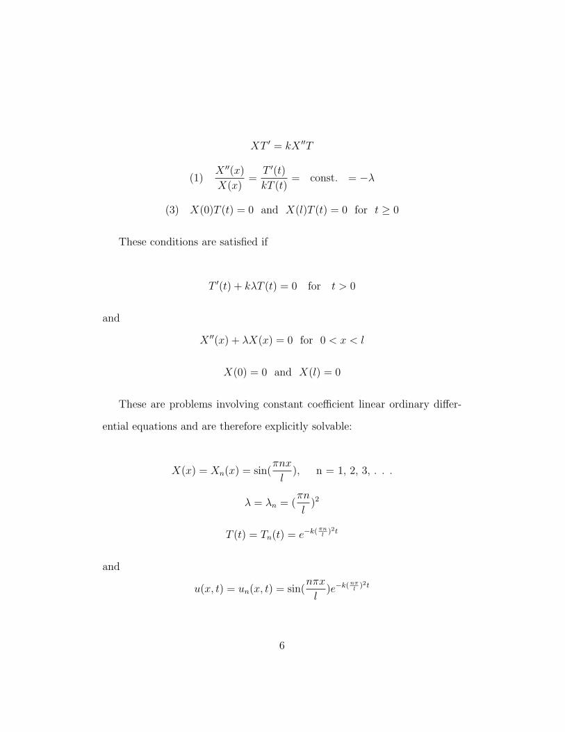
XT ′ = kX ′′T
(1)X ′′(x)
X(x)=
T ′(t)
kT (t)= const. = −λ
(3) X(0)T (t) = 0 and X(l)T (t) = 0 for t ≥ 0
These conditions are satisfied if
T ′(t) + kλT (t) = 0 for t > 0
and
X ′′(x) + λX(x) = 0 for 0 < x < l
X(0) = 0 and X(l) = 0
These are problems involving constant coefficient linear ordinary differ-
ential equations and are therefore explicitly solvable:
X(x) = Xn(x) = sin(πnx
l), n = 1, 2, 3, . . .
λ = λn = (πn
l)2
T (t) = Tn(t) = e−k(πnl
)2t
and
u(x, t) = un(x, t) = sin(nπx
l)e−k(nπ
l)2t
6
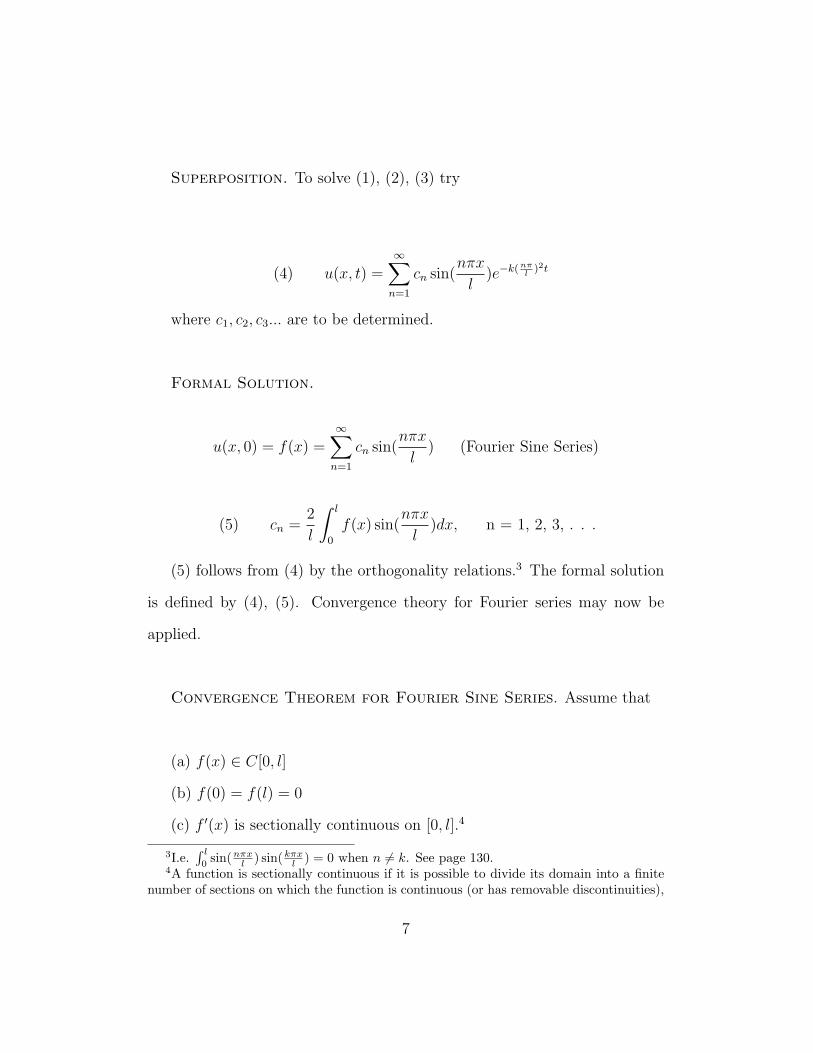
Superposition. To solve (1), (2), (3) try
(4) u(x, t) =∞∑n=1
cn sin(nπx
l)e−k(nπ
l)2t
where c1, c2, c3... are to be determined.
Formal Solution.
u(x, 0) = f(x) =∞∑n=1
cn sin(nπx
l) (Fourier Sine Series)
(5) cn =2
l
∫ l
0
f(x) sin(nπx
l)dx, n = 1, 2, 3, . . .
(5) follows from (4) by the orthogonality relations.3 The formal solution
is defined by (4), (5). Convergence theory for Fourier series may now be
applied.
Convergence Theorem for Fourier Sine Series. Assume that
(a) f(x) ∈ C[0, l]
(b) f(0) = f(l) = 0
(c) f ′(x) is sectionally continuous on [0, l].4
3I.e.∫ l0
sin(nπxl ) sin(kπxl ) = 0 when n 6= k. See page 130.4A function is sectionally continuous if it is possible to divide its domain into a finite
number of sections on which the function is continuous (or has removable discontinuities),
7
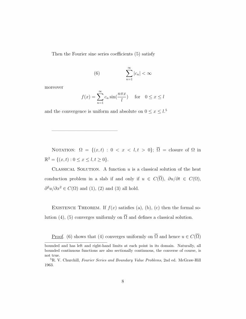
Then the Fourier sine series coefficients (5) satisfy
(6)∞∑n=1
|cn| <∞
moreover
f(x) =∞∑n=1
cn sin(nπx
l) for 0 ≤ x ≤ l
and the convergence is uniform and absolute on 0 ≤ x ≤ l.5
——————————————
Notation: Ω = (x, t) : 0 < x < l, t > 0; Ω = closure of Ω in
R2 = (x, t) : 0 ≤ x ≤ l, t ≥ 0.
Classical Solution. A function u is a classical solution of the heat
conduction problem in a slab if and only if u ∈ C(Ω), ∂u/∂t ∈ C(Ω),
∂2u/∂x2 ∈ C(Ω) and (1), (2) and (3) all hold.
Existence Theorem. If f(x) satisfies (a), (b), (c) then the formal so-
lution (4), (5) converges uniformly on Ω and defines a classical solution.
Proof. (6) shows that (4) converges uniformly on Ω and hence u ∈ C(Ω)
bounded and has left and right-hand limits at each point in its domain. Naturally, allbounded continuous functions are also sectionally continuous, the converse of course, isnot true.
5R. V. Churchill, Fourier Series and Boundary Value Problems, 2nd ed. McGraw-Hill1963.
8
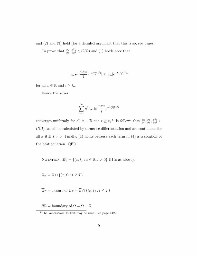
and (2) and (3) hold (for a detailed argument that this is so, see pages .
To prove that ∂u∂t, ∂
2u∂x2 ∈ C(Ω) and (1) holds note that
|cn sinnπx
le−k(nπ
l)2t| ≤ |cn|e−k(nπ
l)2to
for all x ∈ R and t ≥ to.
Hence the series
∞∑n=1
n2cn sinnπx
le−k(nπ
l)2t
converges uniformly for all x ∈ R and t ≥ to.6 It follows that ∂u
∂t, ∂u∂x, ∂
2u∂x2 ∈
C(Ω) can all be calculated by termwise differentiation and are continuous for
all x ∈ R, t > 0. Finally, (1) holds because each term in (4) is a solution of
the heat equation. QED
Notation. R2+ = (x, t) : x ∈ R, t > 0 (Ω is as above).
ΩT = Ω ∩ (x, t) : t < T
ΩT = closure of ΩT = Ω ∩ (x, t) : t ≤ T
∂Ω = boundary of Ω = Ω− Ω
6The Weierstrass M-Test may be used. See page 142-3.
9
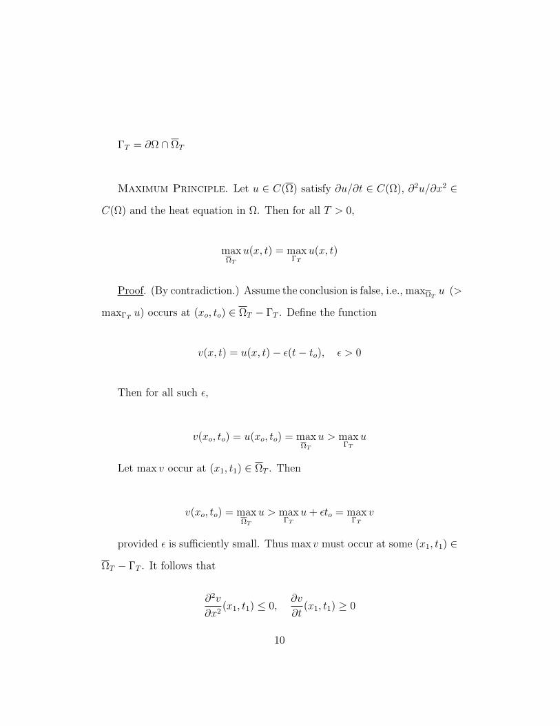
ΓT = ∂Ω ∩ ΩT
Maximum Principle. Let u ∈ C(Ω) satisfy ∂u/∂t ∈ C(Ω), ∂2u/∂x2 ∈
C(Ω) and the heat equation in Ω. Then for all T > 0,
maxΩT
u(x, t) = maxΓT
u(x, t)
Proof. (By contradiction.) Assume the conclusion is false, i.e., maxΩTu (>
maxΓT u) occurs at (xo, to) ∈ ΩT − ΓT . Define the function
v(x, t) = u(x, t)− ε(t− to), ε > 0
Then for all such ε,
v(xo, to) = u(xo, to) = maxΩT
u > maxΓT
u
Let max v occur at (x1, t1) ∈ ΩT . Then
v(xo, to) = maxΩT
u > maxΓT
u+ εto = maxΓT
v
provided ε is sufficiently small. Thus max v must occur at some (x1, t1) ∈
ΩT − ΓT . It follows that
∂2v
∂x2(x1, t1) ≤ 0,
∂v
∂t(x1, t1) ≥ 0
10
whence
∂2u
∂x2(x1, t1) =
∂2v
∂x2(x1, t1) ≤ 0
but
∂u
∂t(x1, t1) =
∂v
∂t(x1, t1) + ε > 0
which contradicts (1) (the heat equation). QED
Uniqueness Theorem. The BV problem (1), (2), (3) can have only
one classical solution.
Proof. Let u1 and u2 be any two classical solutions with the same initial
values f(x). Then u(x, t) = u1(x, t) − u2(x, t) is a classical solution with
f(x) ≡ 0. Thus
maxΩT
u = maxΓT
u = 0
i.e.7
u(x, t) ≤ 0 ∀(x, t) ∈ ΩT
Similarly, −u(x, t) is a classical solution with f(x) ≡ 0. Following the
same reasoning, −u(x, t) ≤ 0. It follows that u(x, t) ≡ 0. QED
7∀ is a logical symbol which simply means “for all.”
11
The maximum principle implies that if f(x) satisfies (a), (b), (c) and
u(x, t) is the corresponding classical solution then
maxΩ|u(x, t)| ≤ max
0≤x≤l|f(x)|
This implies
Continuous Dependence on the Data. Let fn(x) be a sequence
of functions satisfying (a), (b), (c). Let un(x, t) be the corresponding so-
lutions of (1), (2), (3). Suppose further that fn(x)→ 0 uniformly as n→∞
on 0 ≤ x ≤ l. Then un(x, t)→ 0 when n→∞, uniformly in Ω.
12
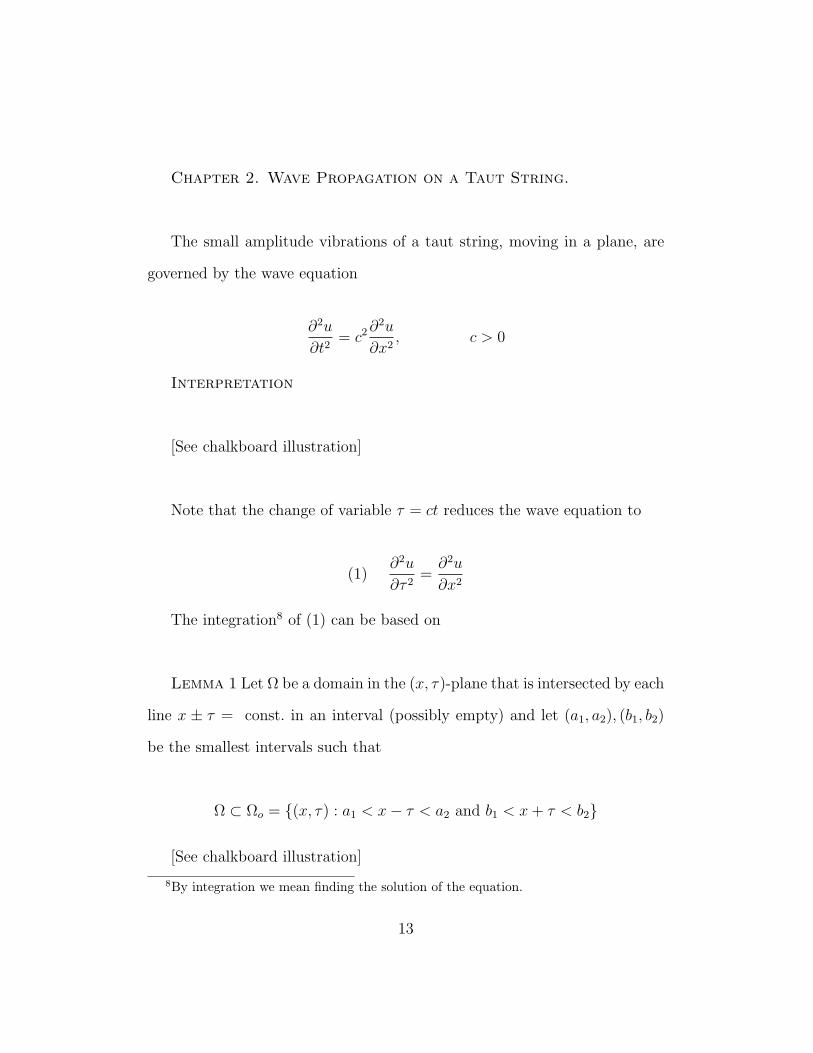
Chapter 2. Wave Propagation on a Taut String.
The small amplitude vibrations of a taut string, moving in a plane, are
governed by the wave equation
∂2u
∂t2= c2∂
2u
∂x2, c > 0
Interpretation
[See chalkboard illustration]
Note that the change of variable τ = ct reduces the wave equation to
(1)∂2u
∂τ 2=∂2u
∂x2
The integration8 of (1) can be based on
Lemma 1 Let Ω be a domain in the (x, τ)-plane that is intersected by each
line x ± τ = const. in an interval (possibly empty) and let (a1, a2), (b1, b2)
be the smallest intervals such that
Ω ⊂ Ωo = (x, τ) : a1 < x− τ < a2 and b1 < x+ τ < b2
[See chalkboard illustration]
8By integration we mean finding the solution of the equation.
13
Assume that u ∈ C2(Ω) and (1) holds for all (x, τ) ∈ Ω. Then there exist
functions f(τ), g(τ) such that
(a) f ∈ C2(a1, a2), g ∈ C2(b1, b2)
(b) u(x, τ) = f(x− τ) + g(x+ τ) in Ω
Remark 1 This is d’Alembert’s solution of (1).
Remark 2 f and g are unique up to constant functions.9
Proof. Introduce new coordinates
ξ = x− τ, η = x+ τ
and let
u(x, τ) = v(ξ, η)
Then (chain rule for partial derivatives)
∂u
∂x=∂v
∂ξ+∂v
∂η,
∂u
∂τ= −∂v
∂ξ+∂v
∂η
∂2u
∂x2=∂2v
∂ξ2+ 2
∂2v
∂ξ∂η+
∂v
∂η2,
∂2u
∂τ 2=∂2u
∂ξ2− 2
∂2v
∂ξ∂η+∂2v
∂η2
9That is, the pair (f, g) is equivalent to the pair (f+C, g−C) where C is any constant.
14
Thus
∂2u
∂x2− ∂2u
∂τ 2= 4
∂2v
∂ξ∂η= 0 in Ω′ = (ξ, η) : (x, τ) ∈ Ω
Also, v ∈ C2(Ω′). Thus for each ηo ∈ (b1, b2), ∂∂ξ
(∂v∂η
) = 0 on a non-empty
ξ-interval (Ω′ is connected) and hence
∂v(ξ, ηo)
∂η= G(ηo) ∈ C1(b1, b2).
Repeating this with ξo ∈ (a1, a2) gives v(ξ, η) = f(ξ) + g(η) on Ω′.
where
g(η) =
∫G(η)dη ∈ C2(b1, b2)
and hence f = v − g ∈ C2(a1, a2). QED
Corollary. Under the hypotheses of Lemma 1 u has an extension
u′ ∈ C2(Ωo) which satisfies (1) in Ωo.
Wave Propagation on a Long String. In the (x, τ) - plane consider
the domains
Ω = (x, τ) : τ > 0, a < x < b,∆ = (x, τ) : τ > 0, τ + a < x < b− τ
15
[See chalkboard illustration]
Let u ∈ C2(Ω) describe a motion of the string. By the lemma the values
of u in ∆ ⊂ ∆o are independent of what happens at the ends of the string
and ∃f, g ∈ C2(a, b)10 such that
u(x, τ) = f(x− τ) + g(x+ τ) in ∆
Moreover, f and g can be determined by the initial values
u(x, 0) = uo(x) and∂u(x, 0)
∂τ= u1(x), a < x < b
Indeed,
u(x, 0) = f(x) + g(x) = uo(x), f ′(x) + g′(x) = u′o(x)
∂u(x, 0)
∂τ= −f ′(x) + g′(x) = u1(x)
Thus
2f ′(x) = u′o(x)− u1(x), 2g′(x) = u′o(x) + u1(x)
2f(x) = uo(x)−∫ x
a
u1(ξ)dξ + C, 2g(x) = uo(x) +
∫ x
a
u1(ξ)dξ + C ′
10∃ is a logical symbol meaning “there exists.”
16
Hence
2(f(x) + g(x)) = 2uo(x) + C + C ′ = 2uo(x)
whence
C + C ′ = 0 or C ′ = −C
Thus
u(x, τ) =1
2uo(x− τ)− 1
2
∫ x−τ
a
u1(ξ)dξ + C
+1
2uo(x+ τ) +
1
2
∫ x+τ
a
u1(ξ)dξ − C
or
(2) u(x, τ) =1
2uo(x− τ) + uo(x+ τ)+
∫ x+τ
x−τu1(ξ)dξ, (x, τ) ∈ ∆.
This leads us to the
Initial Value Problem for the Wave Equation.
In the idealized case of an infinitely long string, a = −∞, b = ∞, (2)
gives the solution of the boundary value problem
17
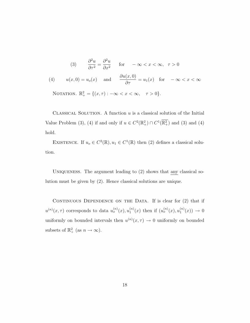
(3)∂2u
∂τ 2=∂2u
∂x2for −∞ < x <∞, τ > 0
(4) u(x, 0) = uo(x) and∂u(x, 0)
∂τ= u1(x) for −∞ < x <∞
Notation. R2+ = (x, τ) : −∞ < x <∞, τ > 0.
Classical Solution. A function u is a classical solution of the Initial
Value Problem (3), (4) if and only if u ∈ C2(R2+) ∩ C1(R2
+) and (3) and (4)
hold.
Existence. If uo ∈ C2(R), u1 ∈ C1(R) then (2) defines a classical solu-
tion.
Uniqueness. The argument leading to (2) shows that any classical so-
lution must be given by (2). Hence classical solutions are unique.
Continuous Dependence on the Data. If is clear for (2) that if
u(n)(x, τ) corresponds to data u(n)o (x), u
(n)1 (x) then if (u
(n)o (x), u
(n)1 (x)) → 0
uniformly on bounded intervals then u(n)(x, τ) → 0 uniformly on bounded
subsets of R2+ (as n→∞).
18
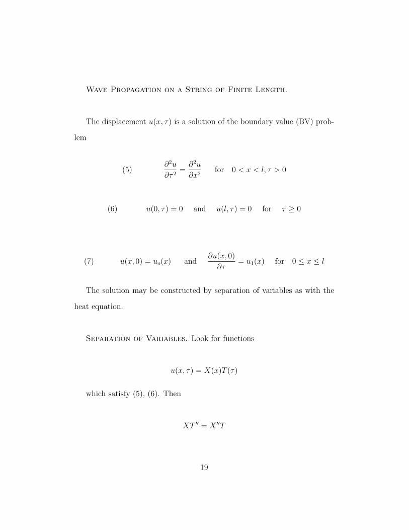
Wave Propagation on a String of Finite Length.
The displacement u(x, τ) is a solution of the boundary value (BV) prob-
lem
(5)∂2u
∂τ 2=∂2u
∂x2for 0 < x < l, τ > 0
(6) u(0, τ) = 0 and u(l, τ) = 0 for τ ≥ 0
(7) u(x, 0) = uo(x) and∂u(x, 0)
∂τ= u1(x) for 0 ≤ x ≤ l
The solution may be constructed by separation of variables as with the
heat equation.
Separation of Variables. Look for functions
u(x, τ) = X(x)T (τ)
which satisfy (5), (6). Then
XT ′′ = X ′′T
19
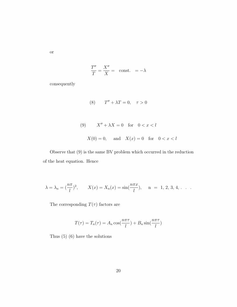
or
T ′′
T=X ′′
X= const. = −λ
consequently
(8) T ′′ + λT = 0, τ > 0
(9) X ′′ + λX = 0 for 0 < x < l
X(0) = 0, and X(x) = 0 for 0 < x < l
Observe that (9) is the same BV problem which occurred in the reduction
of the heat equation. Hence
λ = λn = (nπ
l)2, X(x) = Xn(x) = sin(
nπx
l), n = 1, 2, 3, 4, . . .
The corresponding T (τ) factors are
T (τ) = Tn(τ) = An cos(nπτ
l) +Bn sin(
nπτ
l)
Thus (5) (6) have the solutions
20
un(x, τ) = An cos(nπτ
l) +Bn sin(
nπτ
l) sin(
nπx
l), n = 1, 2, 3, 4, . . .
Principle of Superposition. To solve (5), (6), (7) try
(10) u(x, τ) =∞∑n=1
An cos(nπτ
l) +Bn sin(
nπτ
l) sin(
nπx
l)
∂u(x, τ)
∂τ=∞∑n=1
nπ
l−An sin(
nπτ
l) +Bn cos(
nπτ
l) sin(
nπx
l)
Formal Solution.
u(x, 0) = uo(x) =∞∑n=1
An sin(nπx
l)
∂u(x, 0)
∂τ= u1(x) =
∞∑n=1
nπ
lBn sin(
nπx
l)
Thus
(11) An =2
l
∫ l
0
uo(x) sinnπx
ldx
nπ
lBn =
2
l
∫ l
0
u1(x) sinnπx
ldx n = 1, 2, 3, 4, . . .
The formal solution is defined by (10), (11). We may now proceed to
21
define the
Classical Solution. u is a classical solution of the vibrating string
problem (5), (6), (7) if and only if u ∈ C1(Ω)∩C2(Ω) and (5), (6), (7) hold.
Here Ω = (x, τ) : 0 < x < l, τ > 0, Ω = (x, τ) : 0 ≤ x ≤ l, τ ≥ 0.
The existence of a classical solution can be proved by using convergence
theory for the Fourier sine series, as in the case of the heat equation, but this
does not give the best results (the weakest possible smoothness conditions
on the initial values). Instead Fourier convergence theory will be used in a
different way to sum the formal series (10), (11). For simplicity, only the
special case where
∂u(x, 0)
∂τ= u1(x) ≡ 0
will be discussed. In this case, the formal solution is
(10)′ u(x, τ) =∞∑n=1
An cosnπτ
lsin
nπx
l
(11)′ An =2
l
∫ l
0
uo(x) sinnπx
ldx
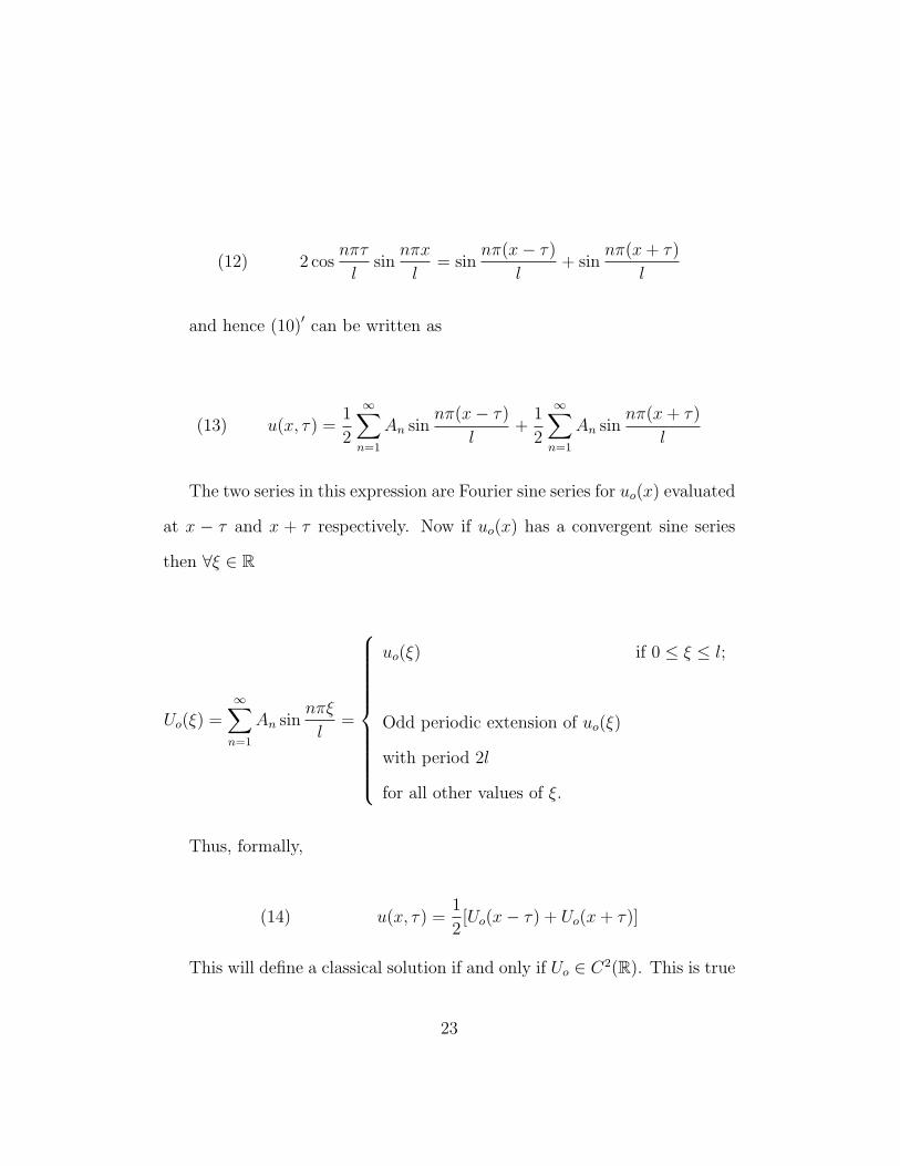
To sum (10)′, (11)′ note that
22
(12) 2 cosnπτ
lsin
nπx
l= sin
nπ(x− τ)
l+ sin
nπ(x+ τ)
l
and hence (10)′ can be written as
(13) u(x, τ) =1
2
∞∑n=1
An sinnπ(x− τ)
l+
1
2
∞∑n=1
An sinnπ(x+ τ)
l
The two series in this expression are Fourier sine series for uo(x) evaluated
at x − τ and x + τ respectively. Now if uo(x) has a convergent sine series
then ∀ξ ∈ R
Uo(ξ) =∞∑n=1
An sinnπξ
l=
uo(ξ) if 0 ≤ ξ ≤ l;
Odd periodic extension of uo(ξ)
with period 2l
for all other values of ξ.
Thus, formally,
(14) u(x, τ) =1
2[Uo(x− τ) + Uo(x+ τ)]
This will define a classical solution if and only if Uo ∈ C2(R). This is true
23
if and only if
(15) uo ∈ C2[0, l]
and
(16) uo(0) = 0, uo(l) = 0, u′′o(0) = 0, u′′o(l) = 011
This proves the
Existence Theorem. If uo satisfies (15), (16) then (13), (14) defines a
classical solution of (5), (6), (7) with u1(x) ≡ 0.
The case where uo(x) ≡ 0 and u1(x) 6= 0 can be treated similarly.
Another Derivation of the Solution Based on Lemma 1
Let u be a classical solution of the finite string problem, i.e.
(1) u ∈ C1(Ω) ∩ C2(Ω) and∂2u
∂τ 2=∂2u
∂x2in Ω
(2) u(x, 0) = uo(x) and∂u(x, 0)
∂τ= u1(x) for 0 ≤ x ≤ l
(3a) u(0, t) = 0 for t ≥ 0
(3b) u(l, t) = 0 for t ≥ 012
11These conditions are necessary to allow a smooth 2l periodic extension of uo.12The conditons (3a), (3b) state that the string is immobilized at the ends.
24
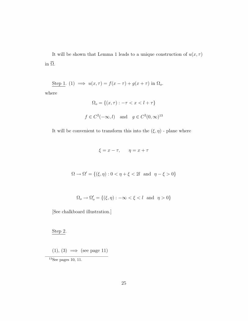
It will be shown that Lemma 1 leads to a unique construction of u(x, τ)
in Ω.
Step 1. (1) =⇒ u(x, τ) = f(x− τ) + g(x+ τ) in Ωo.
where
Ωo = (x, τ) : −τ < x < l + τ
f ∈ C2(−∞, l) and g ∈ C2(0,∞)13
It will be convenient to transform this into the (ξ, η) - plane where
ξ = x− τ, η = x+ τ
Ω→ Ω′ = (ξ, η) : 0 < η + ξ < 2l and η − ξ > 0
Ωo → Ω′o = (ξ, η) : −∞ < ξ < l and η > 0
[See chalkboard illustration.]
Step 2.
(1), (3) =⇒ (see page 11)
13See pages 10, 11.
25
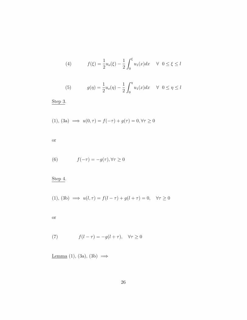
(4) f(ξ) =1
2uo(ξ)−
1
2
∫ ξ
0
u1(x)dx ∀ 0 ≤ ξ ≤ l
(5) g(η) =1
2uo(η)− 1
2
∫ η
0
u1(x)dx ∀ 0 ≤ η ≤ l
Step 3.
(1), (3a) =⇒ u(0, τ) = f(−τ) + g(τ) = 0,∀τ ≥ 0
or
(6) f(−τ) = −g(τ),∀τ ≥ 0
Step 4.
(1), (3b) =⇒ u(l, τ) = f(l − τ) + g(l + τ) = 0, ∀τ ≥ 0
or
(7) f(l − τ) = −g(l + τ), ∀τ ≥ 0
Lemma (1), (3a), (3b) =⇒
26
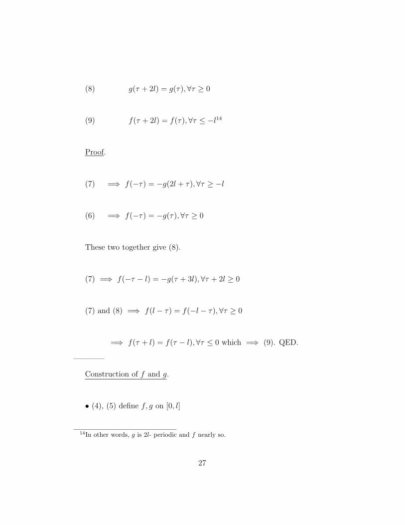
(8) g(τ + 2l) = g(τ),∀τ ≥ 0
(9) f(τ + 2l) = f(τ),∀τ ≤ −l14
Proof.
(7) =⇒ f(−τ) = −g(2l + τ),∀τ ≥ −l
(6) =⇒ f(−τ) = −g(τ),∀τ ≥ 0
These two together give (8).
(7) =⇒ f(−τ − l) = −g(τ + 3l), ∀τ + 2l ≥ 0
(7) and (8) =⇒ f(l − τ) = f(−l − τ),∀τ ≥ 0
=⇒ f(τ + l) = f(τ − l),∀τ ≤ 0 which =⇒ (9). QED.
————
Construction of f and g.
• (4), (5) define f, g on [0, l]
14In other words, g is 2l- periodic and f nearly so.
27
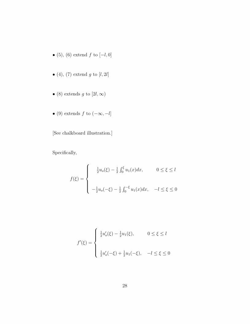
• (5), (6) extend f to [−l, 0]
• (4), (7) extend g to [l, 2l]
• (8) extends g to [2l,∞)
• (9) extends f to (−∞,−l]
[See chalkboard illustration.]
Specifically,
f(ξ) =
12uo(ξ)− 1
2
∫ ξ
0u1(x)dx, 0 ≤ ξ ≤ l
−12uo(−ξ)− 1
2
∫ −ξ0
u1(x)dx, −l ≤ ξ ≤ 0
f ′(ξ) =
12u′o(ξ)− 1
2u1(ξ), 0 ≤ ξ ≤ l
12u′o(−ξ) + 1
2u1(−ξ), −l ≤ ξ ≤ 0
28
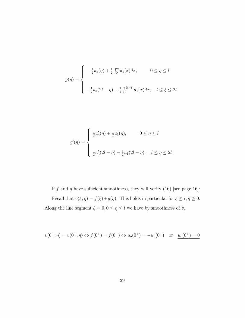
g(η) =
12uo(η) + 1
2
∫ η
0u1(x)dx, 0 ≤ η ≤ l
−12uo(2l − η) + 1
2
∫ 2l−ξ0
u1(x)dx, l ≤ ξ ≤ 2l
g′(η) =
12u′o(η) + 1
2u1(η), 0 ≤ η ≤ l
12u′o(2l − η)− 1
2u1(2l − η), l ≤ η ≤ 2l
If f and g have sufficient smoothness, they will verify (16) [see page 16]:
Recall that v(ξ, η) = f(ξ)+g(η). This holds in particular for ξ ≤ l, η ≥ 0.
Along the line segment ξ = 0, 0 ≤ η ≤ l we have by smoothness of v,
v(0+, η) = v(0−, η)⇔ f(0+) = f(0−)⇔ uo(0+) = −uo(0+) or uo(0
+) = 0
29
∂v(0+, η)
∂ξ=∂v(0−, η)
∂ξ⇔ f ′(0+) = f ′(0−)⇔ u1(0+) = −u1(0+) or u1(0+) = 0
∂2v(0+, η)
∂ξ2=∂2v(0−, η)
∂ξ2⇔ f ′′(0+) = f ′′(0−)⇔ u′′o(0
+) = −u′′o(0+) or u′′o(0+) = 0
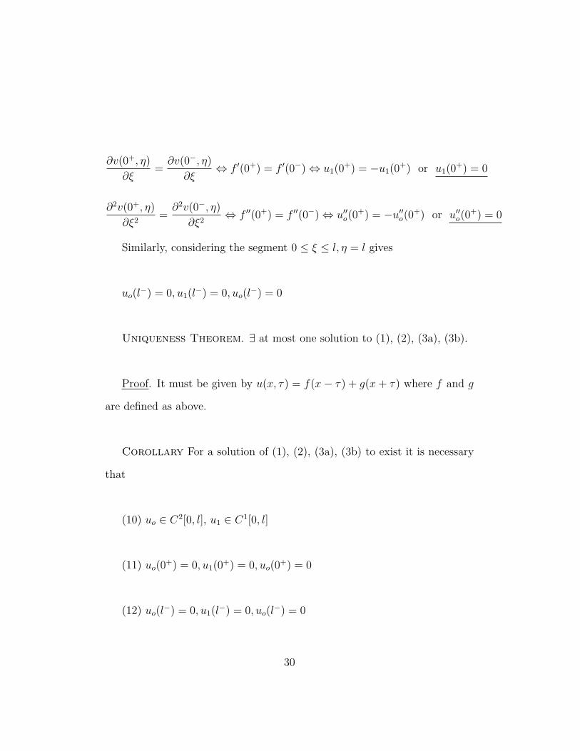
Similarly, considering the segment 0 ≤ ξ ≤ l, η = l gives
uo(l−) = 0, u1(l−) = 0, uo(l
−) = 0
Uniqueness Theorem. ∃ at most one solution to (1), (2), (3a), (3b).
Proof. It must be given by u(x, τ) = f(x− τ) + g(x + τ) where f and g
are defined as above.
Corollary For a solution of (1), (2), (3a), (3b) to exist it is necessary
that
(10) uo ∈ C2[0, l], u1 ∈ C1[0, l]
(11) uo(0+) = 0, u1(0+) = 0, uo(0
+) = 0
(12) uo(l−) = 0, u1(l−) = 0, uo(l
−) = 0
30
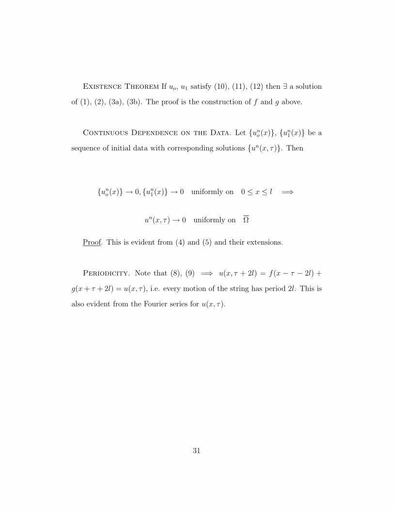
Existence Theorem If uo, u1 satisfy (10), (11), (12) then ∃ a solution
of (1), (2), (3a), (3b). The proof is the construction of f and g above.
Continuous Dependence on the Data. Let uno (x), un1 (x) be a
sequence of initial data with corresponding solutions un(x, τ). Then
uno (x) → 0, un1 (x) → 0 uniformly on 0 ≤ x ≤ l =⇒
un(x, τ)→ 0 uniformly on Ω
Proof. This is evident from (4) and (5) and their extensions.
Periodicity. Note that (8), (9) =⇒ u(x, τ + 2l) = f(x − τ − 2l) +
g(x+ τ + 2l) = u(x, τ), i.e. every motion of the string has period 2l. This is
also evident from the Fourier series for u(x, τ).
31
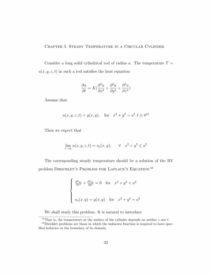
Chapter 3. Steady Temperature in a Circular Cylinder.
Consider a long solid cylindrical rod of radius a. The temperature T =
u(x, y, z, t) in such a rod satisfies the heat equation:
∂u
∂t= K(
∂2u
∂x2+∂2u
∂y2+∂2u
∂z2)
Assume that
u(x, y, z, t) = g(x, y), for x2 + y2 = a2, t ≥ 015
Then we expect that
limt→∞
u(x, y, z, t) = us(x, y), ∀ x2 + y2 ≤ a2
The corresponding steady temperature should be a solution of the BV
problem Dirichlet’s Problem for Laplace’s Equation:16
∂2us∂x2 + ∂2us
∂y2= 0 for x2 + y2 < a2
us(x, y) = g(x, y) for x2 + y2 = a2
We shall study this problem. It is natural to introduce
15That is, the temperature at the surface of the cylinder depends on neither z nor t.16Dirichlet problems are those in which the unknown function is required to have spec-
ified behavior at the boundary of its domain.
32
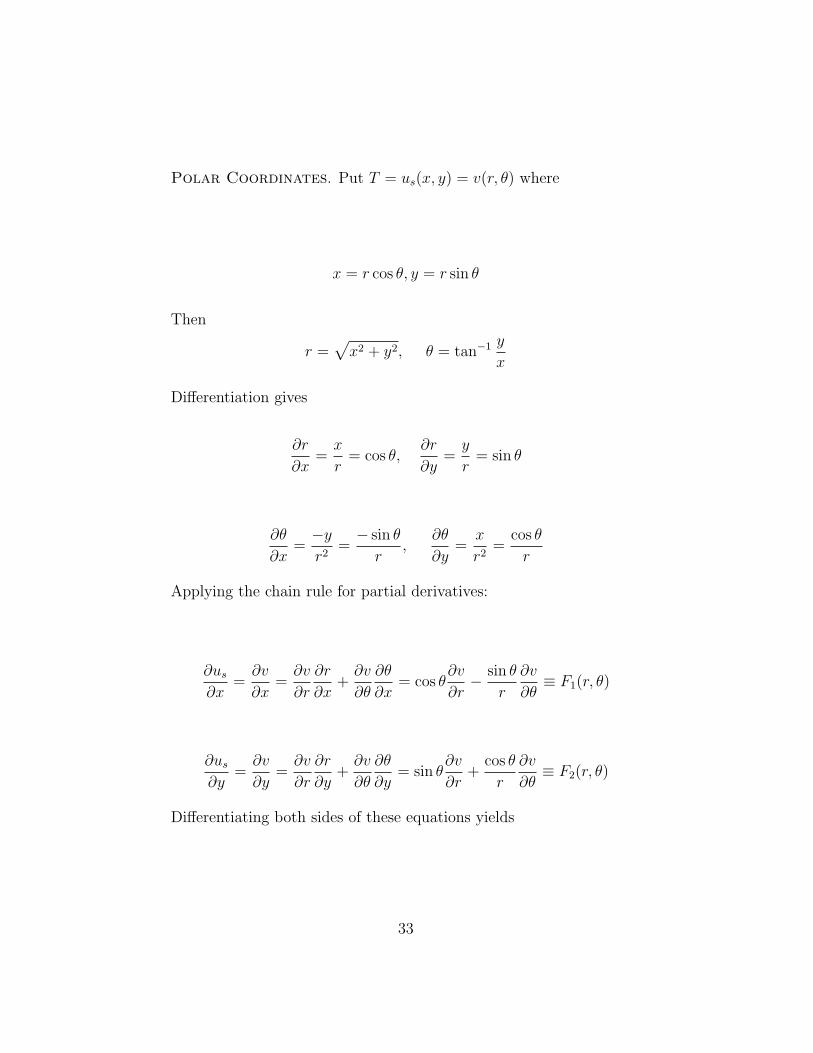
Polar Coordinates. Put T = us(x, y) = v(r, θ) where
x = r cos θ, y = r sin θ
Then
r =√x2 + y2, θ = tan−1 y
x
Differentiation gives
∂r
∂x=x
r= cos θ,
∂r
∂y=y
r= sin θ
∂θ
∂x=−yr2
=− sin θ
r,
∂θ
∂y=
x
r2=
cos θ
r
Applying the chain rule for partial derivatives:
∂us∂x
=∂v
∂x=∂v
∂r
∂r
∂x+∂v
∂θ
∂θ
∂x= cos θ
∂v
∂r− sin θ
r
∂v
∂θ≡ F1(r, θ)
∂us∂y
=∂v
∂y=∂v
∂r
∂r
∂y+∂v
∂θ
∂θ
∂y= sin θ
∂v
∂r+
cos θ
r
∂v
∂θ≡ F2(r, θ)
Differentiating both sides of these equations yields
33
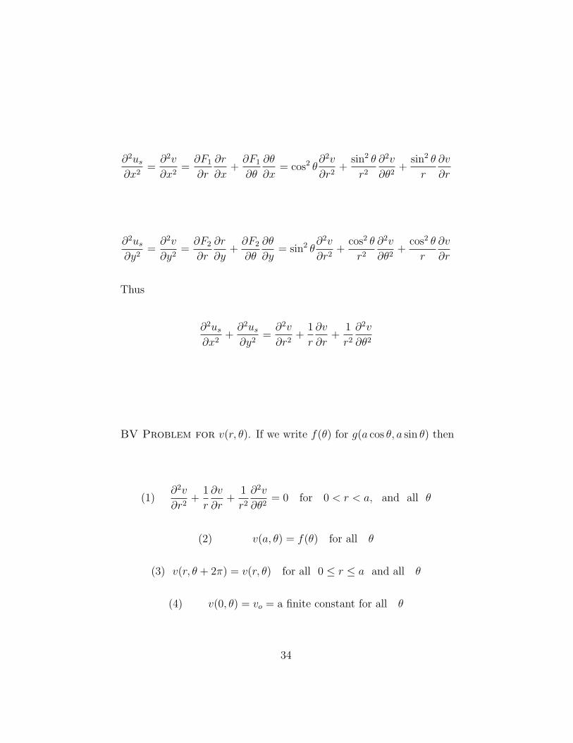
∂2us∂x2
=∂2v
∂x2=∂F1
∂r
∂r
∂x+∂F1
∂θ
∂θ
∂x= cos2 θ
∂2v
∂r2+
sin2 θ
r2
∂2v
∂θ2+
sin2 θ
r
∂v
∂r
∂2us∂y2
=∂2v
∂y2=∂F2
∂r
∂r
∂y+∂F2
∂θ
∂θ
∂y= sin2 θ
∂2v
∂r2+
cos2 θ
r2
∂2v
∂θ2+
cos2 θ
r
∂v
∂r
Thus
∂2us∂x2
+∂2us∂y2
=∂2v
∂r2+
1
r
∂v
∂r+
1
r2
∂2v
∂θ2
BV Problem for v(r, θ). If we write f(θ) for g(a cos θ, a sin θ) then
(1)∂2v
∂r2+
1
r
∂v
∂r+
1
r2
∂2v
∂θ2= 0 for 0 < r < a, and all θ
(2) v(a, θ) = f(θ) for all θ
(3) v(r, θ + 2π) = v(r, θ) for all 0 ≤ r ≤ a and all θ
(4) v(0, θ) = vo = a finite constant for all θ
34
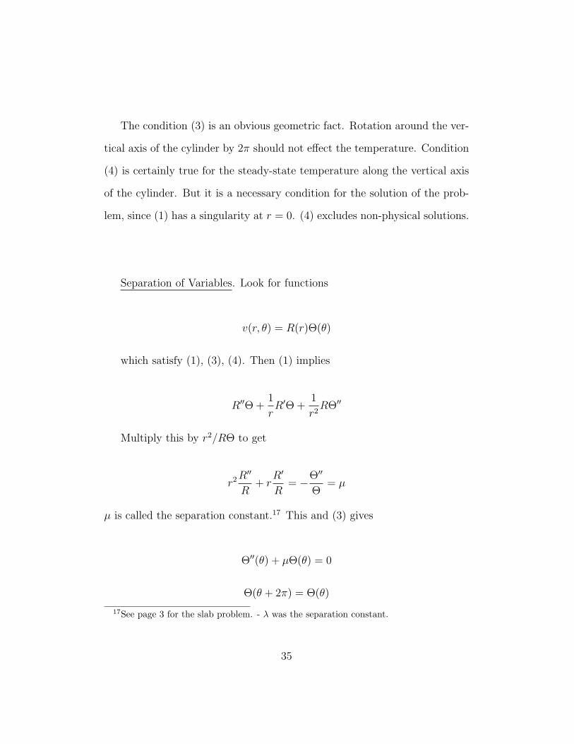
The condition (3) is an obvious geometric fact. Rotation around the ver-
tical axis of the cylinder by 2π should not effect the temperature. Condition
(4) is certainly true for the steady-state temperature along the vertical axis
of the cylinder. But it is a necessary condition for the solution of the prob-
lem, since (1) has a singularity at r = 0. (4) excludes non-physical solutions.
Separation of Variables. Look for functions
v(r, θ) = R(r)Θ(θ)
which satisfy (1), (3), (4). Then (1) implies
R′′Θ +1
rR′Θ +
1
r2RΘ′′
Multiply this by r2/RΘ to get
r2R′′
R+ r
R′
R= −Θ′′
Θ= µ
µ is called the separation constant.17 This and (3) gives
Θ′′(θ) + µΘ(θ) = 0
Θ(θ + 2π) = Θ(θ)
17See page 3 for the slab problem. - λ was the separation constant.
35
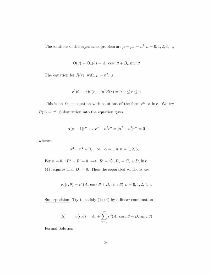
The solutions of this eigenvalue problem are µ = µn = n2, n = 0, 1, 2, 3, ...,
Θ(θ) = Θn(θ) = An cosnθ +Bn sinnθ
The equation for R(r), with µ = n2, is
r2R′′ + rR′(r)− n2R(r) = 0, 0 ≤ r ≤ a
This is an Euler equation with solutions of the form rα or ln r. We try
R(r) = rα. Substitution into the equation gives
α(α− 1)rα + αrα − n2rα = [α2 − n2]rα = 0
whence
α2 − n2 = 0, or α = ±n, n = 1, 2, 3, ...
For n = 0, rR′′ +R′ = 0 =⇒ R′ = Dor, Ro = Co +Do ln r
(4) requires that Do = 0. Thus the separated solutions are
vn(r, θ) = rn(An cosnθ +Bn sinnθ), n = 0, 1, 2, 3, ...
Superposition. Try to satisfy (1)-(4) by a linear combination
(5) v(r, θ) = Ao +∞∑n=1
rn(An cosnθ +Bn sinnθ)
Formal Solution
36
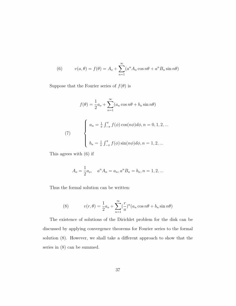
(6) v(a, θ) = f(θ) = Ao +∞∑n=1
(anAn cosnθ + anBn sinnθ)
Suppose that the Fourier series of f(θ) is
f(θ) =1
2ao +
∞∑n=1
(an cosnθ + bn sinnθ)
(7)
an = 1
π
∫ π
−π f(φ) cos(nφ)dφ, n = 0, 1, 2, ...
bn = 1π
∫ π
−π f(φ) sin(nφ)dφ, n = 1, 2, ...
This agrees with (6) if
Ao =1
2ao, anAn = an, a
nBn = bn, n = 1, 2, ...
Thus the formal solution can be written:
(8) v(r, θ) =1
2ao +
∞∑n=1
(r
a)n(an cosnθ + bn sinnθ)
The existence of solutions of the Dirichlet problem for the disk can be
discussed by applying convergence theorems for Fourier series to the formal
solution (8). However, we shall take a different approach to show that the
series in (8) can be summed.
37
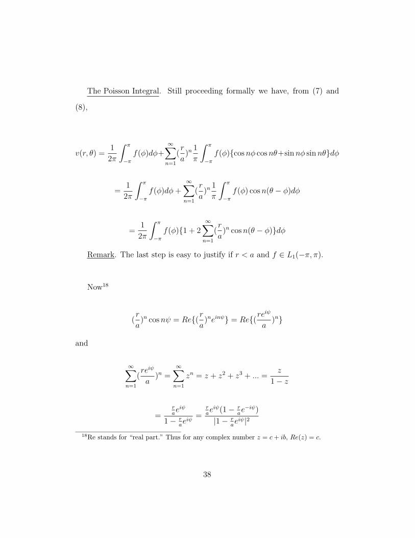
The Poisson Integral. Still proceeding formally we have, from (7) and
(8),
v(r, θ) =1
2π
∫ π
−πf(φ)dφ+
∞∑n=1
(r
a)n
1
π
∫ π
−πf(φ)cosnφ cosnθ+sinnφ sinnθdφ
=1
2π
∫ π
−πf(φ)dφ+
∞∑n=1
(r
a)n
1
π
∫ π
−πf(φ) cosn(θ − φ)dφ
=1
2π
∫ π
−πf(φ)1 + 2
∞∑n=1
(r
a)n cosn(θ − φ)dφ
Remark. The last step is easy to justify if r < a and f ∈ L1(−π, π).
Now18
(r
a)n cosnψ = Re(r
a)neinψ = Re(re
iψ
a)n
and
∞∑n=1
(reiψ
a)n =
∞∑n=1
zn = z + z2 + z3 + ... =z
1− z
=raeiψ
1− raeiψ
=raeiψ(1− r
ae−iψ)
|1− raeiψ|2
18Re stands for “real part.” Thus for any complex number z = c+ ib, Re(z) = c.
38
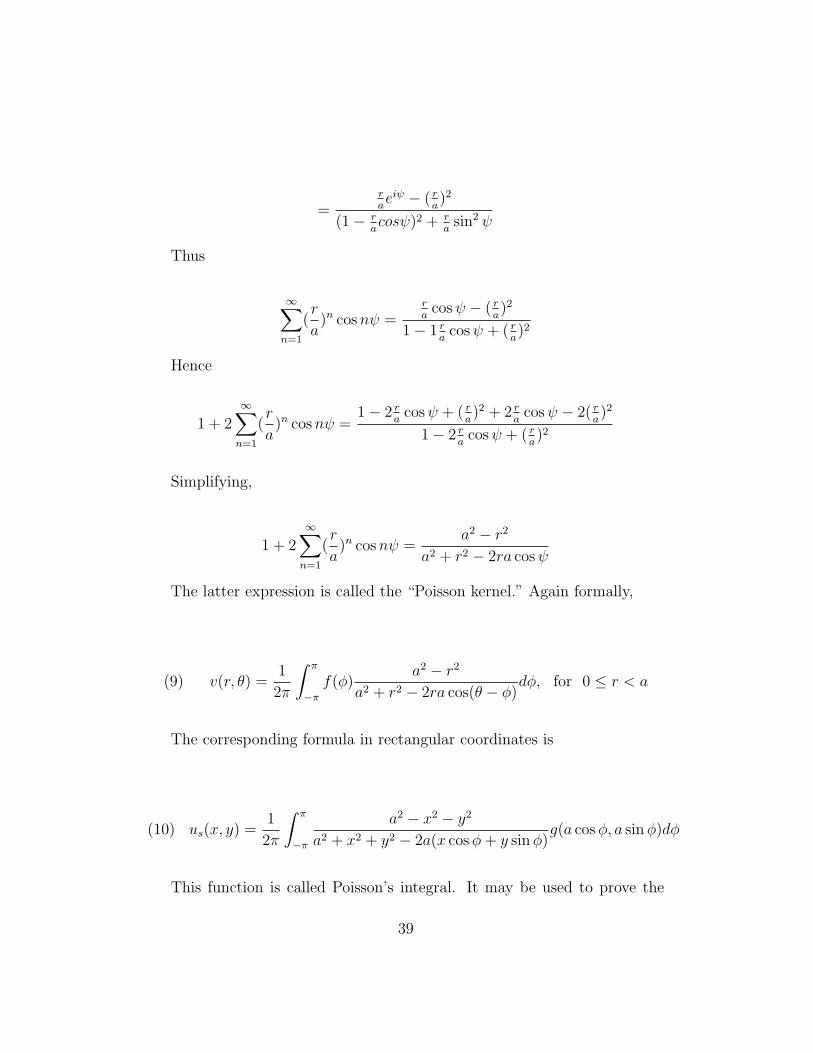
=raeiψ − ( r
a)2
(1− racosψ)2 + r
asin2 ψ
Thus
∞∑n=1
(r
a)n cosnψ =
ra
cosψ − ( ra)2
1− 1 ra
cosψ + ( ra)2
Hence
1 + 2∞∑n=1
(r
a)n cosnψ =
1− 2 ra
cosψ + ( ra)2 + 2 r
acosψ − 2( r
a)2
1− 2 ra
cosψ + ( ra)2
Simplifying,
1 + 2∞∑n=1
(r
a)n cosnψ =
a2 − r2
a2 + r2 − 2ra cosψ
The latter expression is called the “Poisson kernel.” Again formally,
(9) v(r, θ) =1
2π
∫ π
−πf(φ)
a2 − r2
a2 + r2 − 2ra cos(θ − φ)dφ, for 0 ≤ r < a
The corresponding formula in rectangular coordinates is
(10) us(x, y) =1
2π
∫ π
−π
a2 − x2 − y2
a2 + x2 + y2 − 2a(x cosφ+ y sinφ)g(a cosφ, a sinφ)dφ
This function is called Poisson’s integral. It may be used to prove the
39
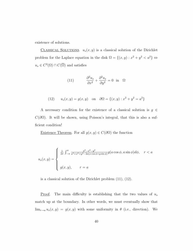
existence of solutions.
Classical Solutions. us(x, y) is a classical solution of the Dirichlet
problem for the Laplace equation in the disk Ω = (x, y) : x2 + y2 < a2 ⇔
us ∈ C2(Ω) ∩ C(Ω) and satisfies
(11)∂2us∂x2
+∂2us∂y2
= 0 in Ω
(12) us(x, y) = g(x, y) on ∂Ω = (x, y) : x2 + y2 = a2
A necessary condition for the existence of a classical solution is g ∈
C(∂Ω). It will be shown, using Poisson’s integral, that this is also a suf-
ficient condition!
Existence Theorem. For all g(x, y) ∈ C(∂Ω) the function
us(x, y) =
1
2π
∫ π
−πa2−x2−y2
a2+x2+y2−2a(x cosφ+y sinφ)g(a cosφ, a sinφ)dφ, r < a
g(x, y), r = a
is a classical solution of the Dirichlet problem (11), (12).
Proof. The main difficulty is establishing that the two values of us
match up at the boundary. In other words, we must eventually show that
limr→a us(x, y) = g(x, y) with some uniformity in θ (i.e., direction). We
40
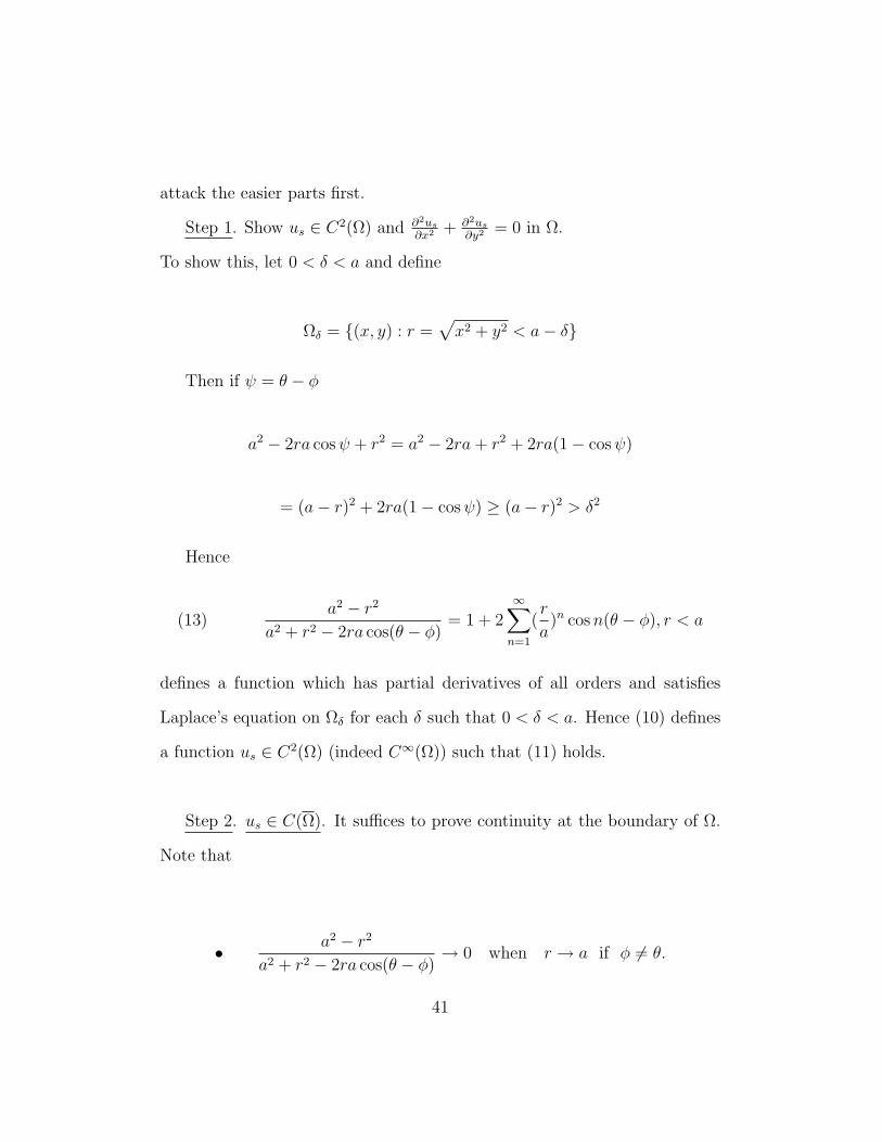
attack the easier parts first.
Step 1. Show us ∈ C2(Ω) and ∂2us∂x2 + ∂2us
∂y2= 0 in Ω.
To show this, let 0 < δ < a and define
Ωδ = (x, y) : r =√x2 + y2 < a− δ
Then if ψ = θ − φ
a2 − 2ra cosψ + r2 = a2 − 2ra+ r2 + 2ra(1− cosψ)
= (a− r)2 + 2ra(1− cosψ) ≥ (a− r)2 > δ2
Hence
(13)a2 − r2
a2 + r2 − 2ra cos(θ − φ)= 1 + 2
∞∑n=1
(r
a)n cosn(θ − φ), r < a
defines a function which has partial derivatives of all orders and satisfies
Laplace’s equation on Ωδ for each δ such that 0 < δ < a. Hence (10) defines
a function us ∈ C2(Ω) (indeed C∞(Ω)) such that (11) holds.
Step 2. us ∈ C(Ω). It suffices to prove continuity at the boundary of Ω.
Note that
• a2 − r2
a2 + r2 − 2ra cos(θ − φ)→ 0 when r → a if φ 6= θ.
41
• a2 − r2
a2 + r2 − 2ra cos(θ − φ)=
a2 − r2
(a− r)2=a+ r
a− r→ +∞ if φ = θ.
• 1
2π
∫ π
−π
a2 − r2
a2 + r2 − 2ra cos(θ − φ)dφ ≡ 1, ∀r < a,−π ≤ θ ≤ π (by 13)
[See chalkboard illustration.]
Thus, for δ > 0 sufficiently small
v(r, θ)− f(θo) =1
2π
∫ π
−π
a2 − r2
a2 + r2 − 2ra cos(θ − φ)f(φ)− f(θo)dφ19
=1
2π
∫ θo+δ
θo−δ
a2 − r2
a2 + r2 − 2ra cos(θ − φ)f(φ)− f(θo)dφ
+1
2π
∫|θo−φ|≥δ
a2 − r2
a2 + r2 − 2ra cos(θ − φ)f(φ)− f(θo)dφ
= I1(r, θ) + I2(r, θ)
Choose δ = δ1(ε) > 0 such that20
|f(φ)− f(θo)| <ε
2∀ φ with |φ− θo| ≤ δ1(ε)
19Recall a2 + r2 − 2ra cos(θ − φ) > 0.20Observe by definition (see (6)) that g(x, y) ∈ C(∂Ω)⇔ f(θ) ∈ C(R) and f(θ+2π) =
f(θ), ∀ θ ∈ R.
42
Then
(15) |I1(r, θ)| ≤ 1
2π
∫ θo+δ
θo−δ
a2 − r2
a2 + r2 − 2ra cos(θ − φ)|f(φ)− f(θo)|dφ
≤ ε
2, ∀θ ∈ R, r < a.
Next observe that
a2 + r2 − 2ra cos(θ − φ) ≥ 2ra(1− cos(θ − φ)) = 4ra sin2 θ − φ2
Take
|θ − θo| <δ1(ε)
2, |θo − φ| ≥ δ1(ε)
Then
|θ − φ| ≥ |θo − φ| − |θ − θo| >δ1(ε)
2
and hence
a2 + r2 − 2ra cos(θ − φ) ≥ 2ra(1− cos(θ − φ) > 4ra sin2 δ1(ε)
4> 0
43
Thus if
M = max0≤θ≤2π
|f(θ)|
|I2(r, θ)| ≤ 1
2π
∫|θo−φ|≥δ1(ε)
a2 − r2
a2 + r2 − 2ra cos(θ − φ)|f(φ)|+ |f(θo)|dφ
(16)
≤ 2M
2π
∫|θo−φ|≥δ1(ε)
a2 − r2
4ra sin2 δ1(ε)4
dφ ≤ 2Ma2 − r2
4ra sin2 δ1(ε)4
<ε
2
provided r > a− δ2(ε) for δ2(ε) sufficiently small, and |θ − θo| < δ1(ε)/2.
Combining (14), (15), (16) gives
|v(r, θ)− f(θo)| ≤ |I1(r, θ)|+ |I2(r, θ)| < ε
∀ (x, y) = (r cos θ, r sin θ) with a− δ2(ε) < r < a, |θ − θo| <δ1(ε)
2.
This shows that us(x, y) − g(xo, yo) → 0 uniformly as (x, y) → (xo, yo)
and this completes the proof. QED.
44
The Mean Value Theorem for Laplace’s Equation. Let
(1) Ω be a domain (any open set) in the (x, y) plane.
(2) u ∈ C2(Ω) and∂2us∂x2
+∂2us∂y2
= 0 in Ω.
(3) D(xo, yo, R) = (x, y) : (x− xo)2 + (y − yo)2 < R2 ⊂ Ω.
Then
(3) u(xo, yo) =1
2π
∫ π
−πu(xo + r cos θ, yo + r sin θ)dθ for 0 ≤ r ≤ R.
In other words, at any point in the domain, u is equal to its mean value
along any circle surrounding it in Ω.
Proof. Define
v(r, θ) = u(xo + r cos θ, yo + r sin θ)
Then
45
(5)∂2v
∂r2+
1
r
∂v
∂r+
1
r2
∂2v
∂θ2= 0 for 0 < r < R, θ ∈ R.
[The reader should check (5) by comparing with pp. 33-34.]
(6) v(r, θ + 2π) = v(r, θ)
Now let
(7) A(r) =1
2π
∫ π
−πv(r, θ)dθ =
1
2π
∫ π
−πu(xo + r cos θ, yo + r sin θ)dθ
Then
A′′(r) +1
rA′(r) =
1
2π
∫ π
−π(∂2
∂r2+
1
r
∂
∂r)v(r, θ)dθ
= − 1
2πr2
∫ π
−π
∂2v
∂θ2dθ = 0 by (5), (6)
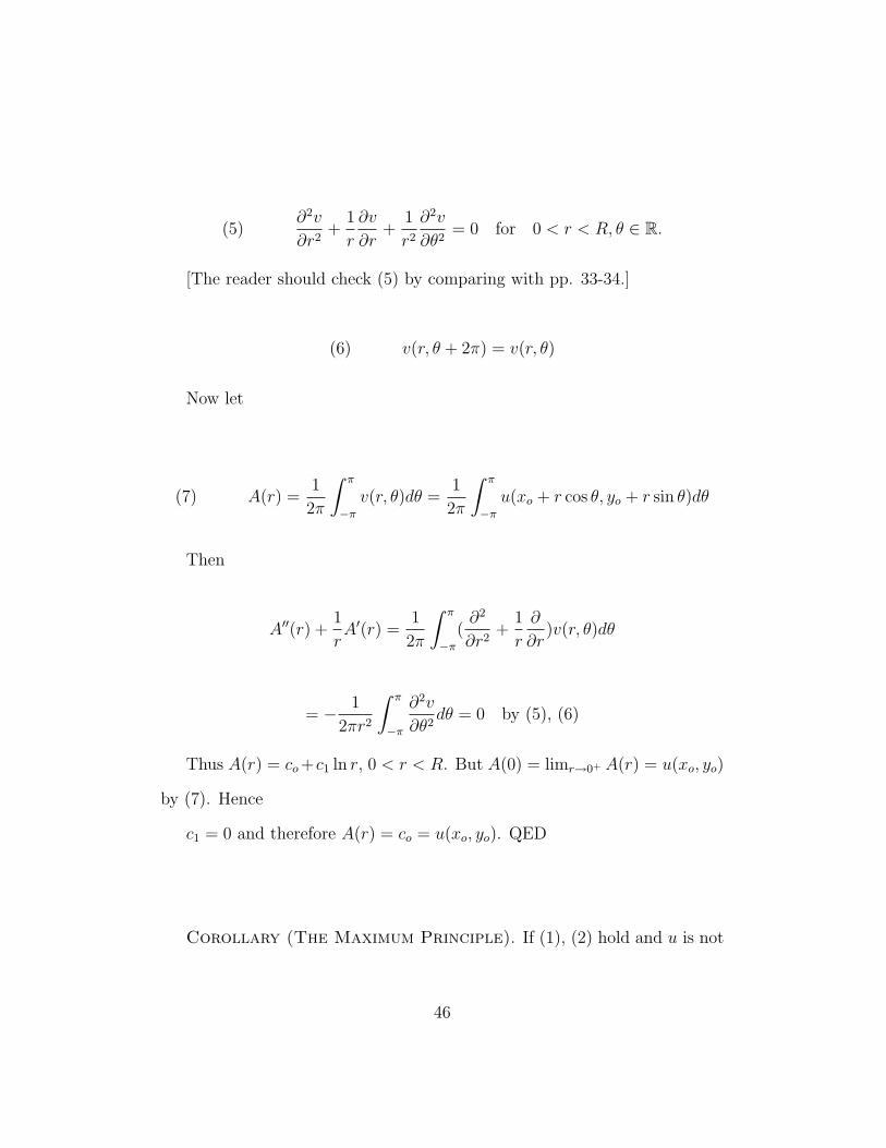
Thus A(r) = co+c1 ln r, 0 < r < R. But A(0) = limr→0+ A(r) = u(xo, yo)
by (7). Hence
c1 = 0 and therefore A(r) = co = u(xo, yo). QED
Corollary (The Maximum Principle). If (1), (2) hold and u is not
46
constant in Ω then it can have no local maximum or minimum in Ω.
Proof. (By contradiction.) Assume u has a local max at (xo, yo) ∈ Ω
then for R sufficiently small, u(x, y) < u(xo, yo) for all (x, y) ∈ D(xo, yo, R)−
(xo, yo). This violates (3).
Corollary. If Ω is compact,
u ∈ C(Ω) ∩ C2(Ω)
and
∂2u
∂x2+∂2u
∂y2= 0 in Ω
then the maximum and minimum of u occur on ∂Ω.
Uniqueness Theorem. If Ω is compact then the Dirichlet problem
for Laplace’s equation in Ω has at most one classical solution. Proof. Let
u1(x, y) and u2(x, y) be any two solutions with the same values on ∂Ω. Then
u(x, y) = u1(x, y)−u2(x, y) satisfies the conditions of the preceding corollary
and vanishes on ∂Ω. Hence u(x, y) ≡ 0 on Ω or
u1(x, y) ≡ u2(x, y)
QED.
47
Chapter 4. Basic Concepts in the Theory of Heat Conduc-
tion.
Temperature. The notion of the temperature of a body (at a point) is an
intuitive concept. A more precise definition can be based on thermodynam-
ics. In any case it is measurable by thermometers, thermocouples and many
other devices, The temperature relative to a fixed scale is measured by a real
number. Scales include
• Centigrade or Celsius Scale TC = 0 ↔ Freezing water.
• Fahrenheit Scale TF = 32 + 9/5TC
• Kelvin (or Absolute) Scale TK = TC + 273.16
The Kelvin scale is derived from thermodynamic principles. It has the
property that every body has a temperature
TK ≥ 0
Quantity of Heat. Heat is a form of energy. The basic unit of heat energy
is the calory (also spelled calorie), defined by the property that 1 calory =
Quantity of heat needed to heat 1 gram of water from 14.5C to 15.5C.
Specific Heat of a Solid. The lower case c will be used to represent this
48
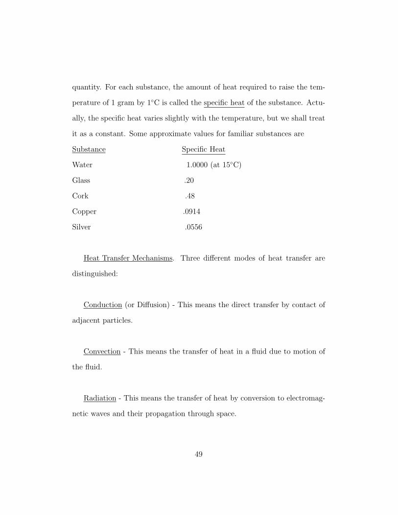
quantity. For each substance, the amount of heat required to raise the tem-
perature of 1 gram by 1C is called the specific heat of the substance. Actu-
ally, the specific heat varies slightly with the temperature, but we shall treat
it as a constant. Some approximate values for familiar substances are
Substance Specific Heat
Water 1.0000 (at 15C)
Glass .20
Cork .48
Copper .0914
Silver .0556
Heat Transfer Mechanisms. Three different modes of heat transfer are
distinguished:
Conduction (or Diffusion) - This means the direct transfer by contact of
adjacent particles.
Convection - This means the transfer of heat in a fluid due to motion of
the fluid.
Radiation - This means the transfer of heat by conversion to electromag-
netic waves and their propagation through space.
49
In solid bodies heat transfer in the interior is assumed to take place by
pure conduction. It may be necessary to consider convection and/or radia-
tion at the surface of a solid.
The Physical Principles Governing Heat Conduction.
There are two principles
I. The Conservation of Heat Energy. This is usually formulated as the
statement that if V is any volume in a solid then
Net Change in quantity of heat in V during any time interval =
Net Flux of heat through the surface of V during the same time interval.
This statement will be quantified below in several cases.
II. Fourier’s Law of Heat Conduction. This states that the rate of flow of
heat at any point in a solid is a function of the temperature gradient at that
point.
This will also be quantified in several different cases below. To begin, the
case of 1-dimensional heat flow in a plate (slab) is discussed.
50
Heat Flow in a Plate. Imagine a large uniform plate (or wall) with
Area = A, Thickness = l.
Assume that the two faces are kept at fixed temperature To and T1 6= To,
T (x) being the temperature (independent of time) on a plane parallel to the
faces of the plate at depth x21 and let
Q = Quantity of heat in the plate from
side 0 to side 1 in t units of time.22
In this case Fourier’s law states that
Q ∝ (T1 − To)A
l
Thus one may write
(1) Q = −K (T1 − To)Atl
where the constant of proportionality K = the thermal conductivty of the
21Hence To = T (0), T1 = T (l).22Therefore the quantity of heat in the plate between x = 0 and some interior depth
x = xo would be Q(xo, t) = − (T (xo)−To)Atl .
51
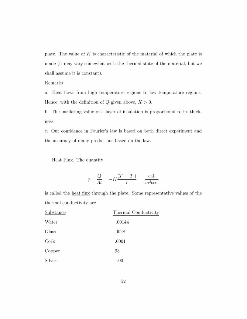
plate. The value of K is characteristic of the material of which the plate is
made (it may vary somewhat with the thermal state of the material, but we
shall assume it is constant).
Remarks
a. Heat flows from high temperature regions to low temperature regions.
Hence, with the definition of Q given above, K > 0.
b. The insulating value of a layer of insulation is proportional to its thick-
ness.
c. Our confidence in Fourier’s law is based on both direct experiment and
the accuracy of many predictions based on the law.
Heat Flux. The quantity
q =Q
At= −K (T1 − To)
l
cal.
m2sec.
is called the heat flux through the plate. Some representative values of the
thermal conductivity are
Substance Thermal Conductivity
Water .00144
Glass .0028
Cork .0001
Copper .93
Silver 1.00
52
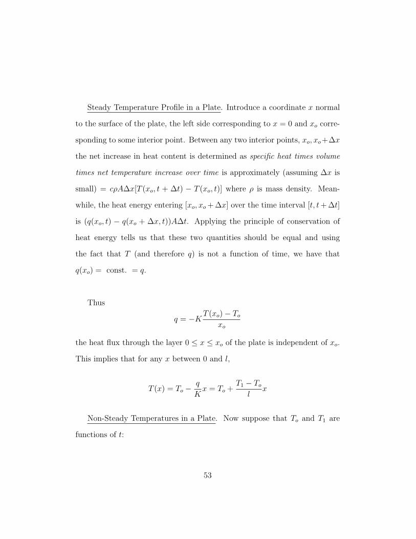
Steady Temperature Profile in a Plate. Introduce a coordinate x normal
to the surface of the plate, the left side corresponding to x = 0 and xo corre-
sponding to some interior point. Between any two interior points, xo, xo+∆x
the net increase in heat content is determined as specific heat times volume
times net temperature increase over time is approximately (assuming ∆x is
small) = cρA∆x[T (xo, t + ∆t) − T (xo, t)] where ρ is mass density. Mean-
while, the heat energy entering [xo, xo + ∆x] over the time interval [t, t+ ∆t]
is (q(xo, t) − q(xo + ∆x, t))A∆t. Applying the principle of conservation of
heat energy tells us that these two quantities should be equal and using
the fact that T (and therefore q) is not a function of time, we have that
q(xo) = const. = q.
Thus
q = −KT (xo)− Toxo
the heat flux through the layer 0 ≤ x ≤ xo of the plate is independent of xo.
This implies that for any x between 0 and l,
T (x) = To −q
Kx = To +
T1 − Tol
x
Non-Steady Temperatures in a Plate. Now suppose that To and T1 are
functions of t:
53
To = To(t), T1 = T1(t)
In this case the temperature in the plate will be a function of t and x,
the coordinate introduced above:
T = T (x, t), 0 ≤ x ≤ l
Consider the very thin slab parallel to the plate
Fourier’s law for steady temperatures suggests that the instantaneous flux
of heat through this slab, at time t, is approximately
q(xo, t) ' −KT (xo + ∆x, t)− T (xo, t)
∆x' −K∂T (xo, t)
∂x
Fourier assumed this law was exact in the limit as ∆x→ 0.
Fourier’s Law of Transient Heat Flow (1 Dimension)
q(xo, t) = −K∂T (xo, t)
∂x
As in the case of steady heat flow, our confidence in Fourier’s law is based
on the accuracy of many predictions based on it.
The Heat Equation for Non-Steady Temperatures in a Plate. Apply the
54
conservation of energy principle to a portion (x, x + ∆x) of the plate and a
time interval (t, t+ ∆t):
The net increase of heat content of (x, x+ ∆x) during (t, t+ ∆t)
= c
mass︷ ︸︸ ︷ρ A∆x︸ ︷︷ ︸
volume
[T (x, t+ ∆t)− T (x, t)︸ ︷︷ ︸net temperature increase
]
The heat energy entering (x, x+ ∆x) during (t, t+ ∆t) is
∫ t+∆t
t
Aq(x, t)dt︸ ︷︷ ︸heat entering at x
−∫ t+∆t
t
Aq(x+ ∆x, t)dt︸ ︷︷ ︸heat leaving at x+∆x
= −A∫ t+∆t
t
∫ x+∆x
x
∂q
∂xdt
By conservation of energy the two quantities are equal and thus,
−A∫ t+∆t
t
∫ x+∆x
x
∂q
∂xdt = cρA∆x[T (x, t+ ∆t)− T (x, t)]
or
− 1
∆t
∫ t+∆t
t
1
∆x
∫ x+∆x
x
∂q
∂xdt = cρ
T (x, t+ ∆t)− T (x, t)
∆t
Making ∆t,∆x→ 0 gives
−∂q(x, t)∂x
= cρ∂T (x, t)
∂t
Applying Fourier’s law,
55
K∂2T
∂x2= cρ
∂T
∂t
or
∂T
∂t= k
∂2T
∂x2
where
k = Kcρ
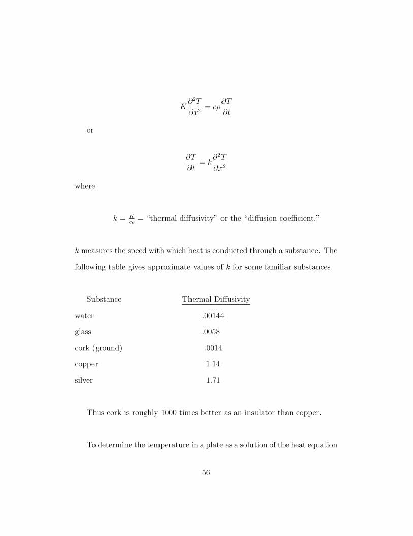
= “thermal diffusivity” or the “diffusion coefficient.”
k measures the speed with which heat is conducted through a substance. The
following table gives approximate values of k for some familiar substances
Substance Thermal Diffusivity
water .00144
glass .0058
cork (ground) .0014
copper 1.14
silver 1.71
Thus cork is roughly 1000 times better as an insulator than copper.
To determine the temperature in a plate as a solution of the heat equation
56
we must know T at some initial time (say t = 0). This gives
Initial Condition.
T (x, 0) = f(x) (a given function) for 0 ≤ x ≤ l
Boundary Conditions. In addition the temperatures at the two faces of
the plate must be controlled in some way. Several possibilities will be con-
sidered.
Surface Temperatures Given:
T (0, t) = To(t) (a given function) fort ≥ 0
T (l, t) = T1(t) (a given function) for t ≥ 0
Surface Heat Flux Given. Instead of specifying the surface temperatures
one may specify
q(0, t) = −K∂T (0, t)
∂x= qo(t) (a given function) t ≥ 0
or
57
∂T (0, t)
∂x= go(t) (=
qo(t)
−K) for t ≥ 0
Similarly
∂T (l, t)
∂x= g1(t) for t ≥ 0
may be given.
Convection Boundary Condition. If the plate face at x = 0 is cooled by
convection into a fluid at temperature Te then, to a good approximation,
−q(0, t) = K∂T (0, t)
∂x= H(T (0, t)− Te)
where H = “outer conductivity” = const.
Thus
∂T (0, t)
∂x− hT (0, t) = −hTe, t ≥ 0
where h = H/K. Note that since heat flows from hot to cold, H ≥ 0, h ≥ 0.
Mixed Boundary Conditions. We can have one of the above conditions
at x = 0 and a different one at x = l.
Linear Diffusion of Heat in a Slender Non-Uniform Rod.
In this context “slender” means that the temperature in the rod can be de-
58
scribed by a function
T = T (x, t)
where x measures distance along the rod.
[See blackboard illustration.]
The physical characteristics of the rod are described by the real-valued
positive functions
A = A(x) = cross-sectional area of rod
P = P (x) = perimeter of rod
ρ = ρ(x) = linear density of rod
c = c(x) = specific heat of rod
K = K(x) = thermal conductivity of rod
H = H(x) = outer conductivity of rod
If the rod is cooling through its surface into an environment with tem-
perature Te(x) then (cf. p. 59)
Net heat energy entering (x, x+ ∆x) during (t, t+ ∆t)
= −∫ t+∆t
t
[A(x+ ∆x)q(x+ ∆x, t)− A(x)q(x, t)]dt
59
−∫ x+∆x
x
∫ t+∆t
t
H(x)[T (x, t)− Te(x)]P (x)dtdx
and
Net increase in heat content of (x, x+∆x) during (t, t+∆t) (assuming ∆x is small)
= c(x)ρ(x)A(x)∆x[T (x, t+ ∆t)− T (x, t)]
Equating these and dividing by ∆x∆t gives
− 1
∆t
∫ t+∆t
t
[A(x+ ∆x)q(x+ ∆x, t)− A(x)q(x, t)]
∆xdt
− 1
∆x
∫ x+∆x
x
1
∆t
∫ t+∆t
t
H(x)[T (x, t)− Te(x)]P (x)dtdx
= c(x)ρ(x)A(x)[T (x, t+ ∆t)− T (x, t)
∆t]
Making ∆x,∆t→ 0 gives
− ∂
∂x(A(x)q(x, t))−H(x)P (x)[T (x, t)− Te(x)] = c(x)ρ(x)
∂T (x, t)
∂t
60
Combining this and Fourier’s law for a non-uniform rod:
q(x, t) = −K(x)∂T (x, t)
∂x
gives the heat diffusion equation for a slender non-uniform rod:
c(x)ρ(x)A(x)∂T
∂t=
∂
∂x(A(x)K(x)
∂T
∂x)−H(x)P (x)[T (x, t)− Te(x)]
This has the form
∂T
∂t− LT = F (x)
where F (x) is a known function and
Lu = po(x)∂2u
∂x2+ p1(x)
∂u
∂x+ p2(x)u
with
po(x) =K(x)
c(x)ρ(x)> 0
p1(x) =1
ρ(x)c(x)A(x)
d
dx(A(x)K(x))
p2(x) = − H(x)P (x)
ρ(x)c(x)A(x)< 0
61
It is interesting that the most general linear second order operator23 L
can arise in this way; i.e., by suitable choice of A(x), P (x), etc. The only
restrictions are that po(x) > 0, p2(x) < 0.
The initial and boundary conditions given on pp. 58-59 are appropriate
for the non-uniform rod. In addition we will consider the
Fourier Ring Problem. Imagine bending a slender rod of length l into a
ring and joining the ends. Then the physical identity of the ends x = 0 and
x = l gives the
Periodic Boundary Condition.
T (0, t) = T (l, 0) and K(0)∂T (0, t)
∂x= K(l)
∂T (l, t)
∂x, t ≥ 0
23See appendix I.
62
Diffusion of Heat in 3 Space Dimensions. Consider a heat con-
ducting solid body occupying a domain Ω ⊂ R3. The thermal state of the
body is characterized by a temperature field
T = T (x, t), x = (x1, x2, x3) ∈ Ω
(x is a vector quantity).
Let c = c(x) = the specific heat of the body at x ∈ Ω.
ρ = ρ(x) = density of the body at x ∈ Ω.
Thus if V ⊂ Ω is any volume in the body
Q(t) =
∫V
c(x)ρ(x)T (x, t)dx = Total quantity of heat in V at time t
where dx = dx1dx2dx3.24 In the important case where the body is homo-
geneous c and ρ are constants and Q(t) = cρ∫VT (x, t)dx.
The flow of heat in the body is described by a vector field
~q(x, t) = (q1(x, t), q2(x, t), q3(x, t)) = Heat Flux Field
24The single integral sign is customary in modern mathematics. In elementary calculusone often sees multiple integral signs corresponding to the space dimension.
63
To interpret ~q let dS be a (small) surface element in Ω with unit normal
vector ~ν.
[See blackboard illustration.]
Then
~q(x, t) • ~ν(x)dS = Quantity of heat crossing dS per unit time at time t
In particular, if V is any volume inside the body with boundary ∂V having
exterior unit normal ~ν(x) then the surface integral
∫∂V
~q(x, t) • ~ν(x)dS = Quantity of heat leaving V per unit time at time t.
Conservation of Heat Energy. The conservation of heat energy law be-
comes, in this context the statement
∫∂V
~q(x, t) • ~ν(x)dS = −dQdt
To obtain a differential equation we can use the divergence theorem:
64
∫V
∇ • ~Adx =
∫∂V
~ν • ~AdS
or
∫V
(∂A1
∂x1
+∂A2
∂x2
+∂A3
∂x3
)dx1dx2dx3 =
∫∂V
(ν1A1 + ν2A2 + ν3A3)dS
Applying this to ~q gives
∫V
∇ • ~qdx =
∫∂V
~ν • ~qdS
Hence the conservation of heat energy principle can be written
∫V
∇ • ~qdx = −∫V
c(x)ρ(x)∂T (x, t)
∂tdx
or
∫V
∇ • ~qdx+ c(x)ρ(x)∂T (x, t)
∂tdx = 0
If T (x, t), ~q(x, t) are C1 functions (in Ω×R) and c(x), ρ(x) ∈ C1(Ω) then
the integrand in the last integral is continuous in Ω (for any fixed t). Since
the identity holds for all volumes V ⊂ Ω it follows that
(1) ∇ • ~q + c(x)ρ(x)∂T (x, t)
∂t= 0, x ∈ Ω, t ∈ R
65
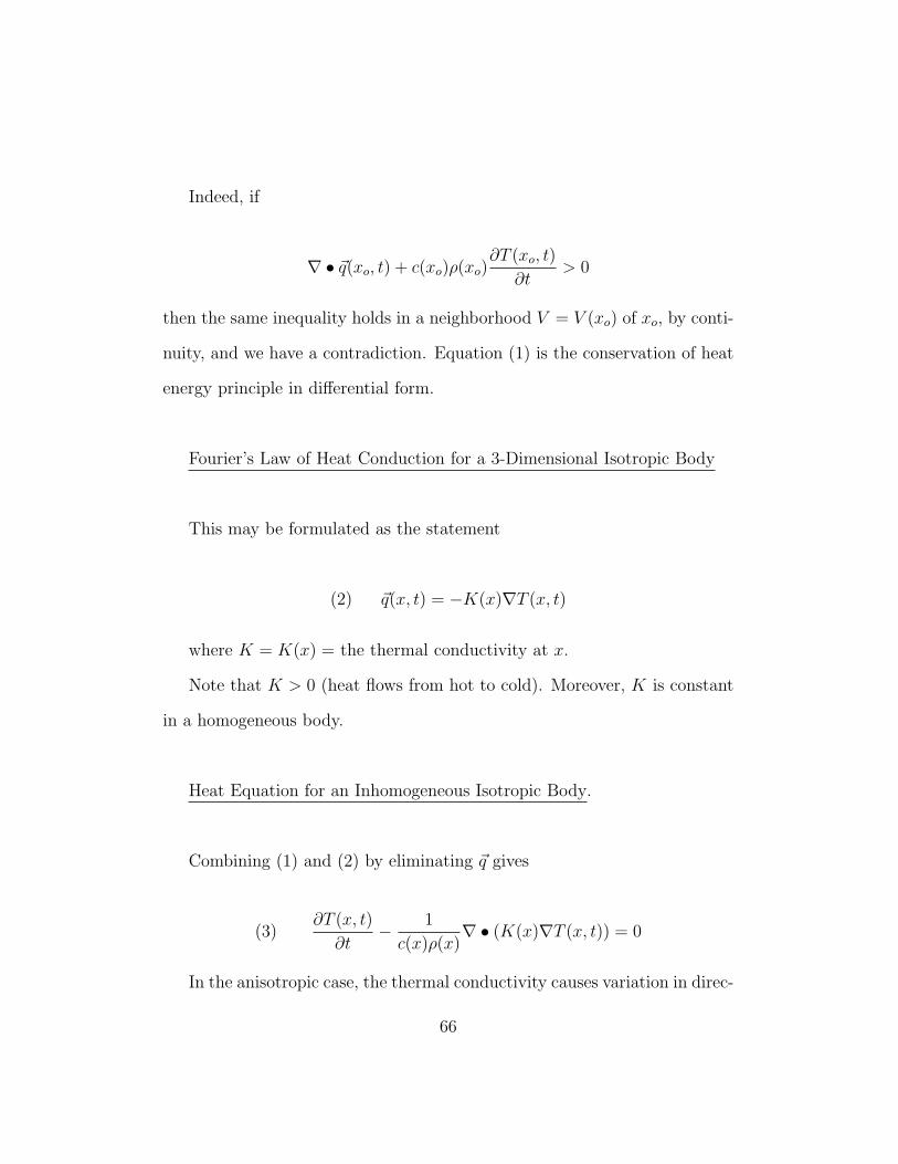
Indeed, if
∇ • ~q(xo, t) + c(xo)ρ(xo)∂T (xo, t)
∂t> 0
then the same inequality holds in a neighborhood V = V (xo) of xo, by conti-
nuity, and we have a contradiction. Equation (1) is the conservation of heat
energy principle in differential form.
Fourier’s Law of Heat Conduction for a 3-Dimensional Isotropic Body
This may be formulated as the statement
(2) ~q(x, t) = −K(x)∇T (x, t)
where K = K(x) = the thermal conductivity at x.
Note that K > 0 (heat flows from hot to cold). Moreover, K is constant
in a homogeneous body.
Heat Equation for an Inhomogeneous Isotropic Body.
Combining (1) and (2) by eliminating ~q gives
(3)∂T (x, t)
∂t− 1
c(x)ρ(x)∇ • (K(x)∇T (x, t)) = 0
In the anisotropic case, the thermal conductivity causes variation in direc-
66
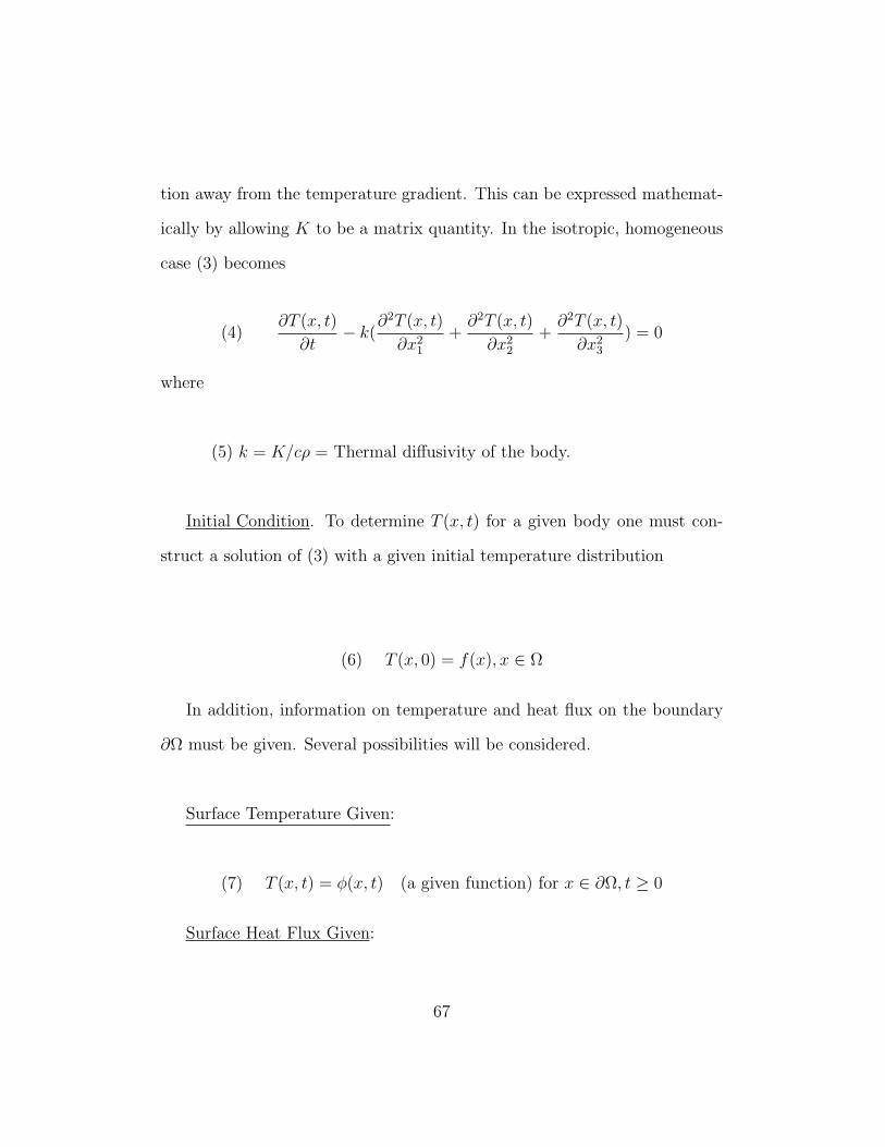
tion away from the temperature gradient. This can be expressed mathemat-
ically by allowing K to be a matrix quantity. In the isotropic, homogeneous
case (3) becomes
(4)∂T (x, t)
∂t− k(
∂2T (x, t)
∂x21
+∂2T (x, t)
∂x22
+∂2T (x, t)
∂x23
) = 0
where
(5) k = K/cρ = Thermal diffusivity of the body.
Initial Condition. To determine T (x, t) for a given body one must con-
struct a solution of (3) with a given initial temperature distribution
(6) T (x, 0) = f(x), x ∈ Ω
In addition, information on temperature and heat flux on the boundary
∂Ω must be given. Several possibilities will be considered.
Surface Temperature Given:
(7) T (x, t) = φ(x, t) (a given function) for x ∈ ∂Ω, t ≥ 0
Surface Heat Flux Given:
67
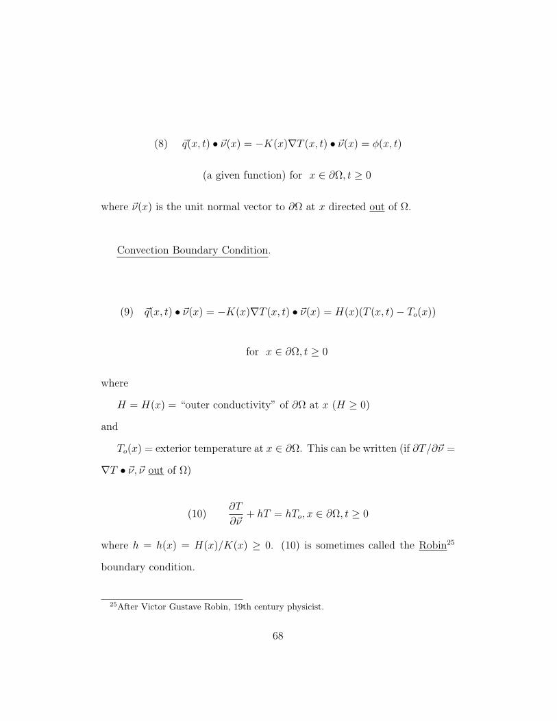
(8) ~q(x, t) • ~ν(x) = −K(x)∇T (x, t) • ~ν(x) = φ(x, t)
(a given function) for x ∈ ∂Ω, t ≥ 0
where ~ν(x) is the unit normal vector to ∂Ω at x directed out of Ω.
Convection Boundary Condition.
(9) ~q(x, t) • ~ν(x) = −K(x)∇T (x, t) • ~ν(x) = H(x)(T (x, t)− To(x))
for x ∈ ∂Ω, t ≥ 0
where
H = H(x) = “outer conductivity” of ∂Ω at x (H ≥ 0)
and
To(x) = exterior temperature at x ∈ ∂Ω. This can be written (if ∂T/∂~ν =
∇T • ~ν, ~ν out of Ω)
(10)∂T
∂~ν+ hT = hTo, x ∈ ∂Ω, t ≥ 0
where h = h(x) = H(x)/K(x) ≥ 0. (10) is sometimes called the Robin25
boundary condition.
25After Victor Gustave Robin, 19th century physicist.
68
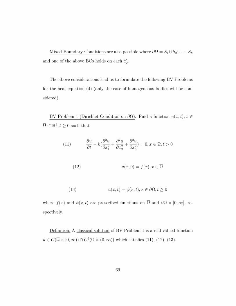
Mixed Boundary Conditions are also possible where ∂Ω = S1∪S2∪. . . Sk
and one of the above BCs holds on each Sj.
The above considerations lead us to formulate the following BV Problems
for the heat equation (4) (only the case of homogeneous bodies will be con-
sidered).
BV Problem 1 (Dirichlet Condition on ∂Ω). Find a function u(x, t), x ∈
Ω ⊂ R3, t ≥ 0 such that
(11)∂u
∂t− k(
∂2u
∂x21
+∂2u
∂x22
+∂2u
∂x23
) = 0, x ∈ Ω, t > 0
(12) u(x, 0) = f(x), x ∈ Ω
(13) u(x, t) = φ(x, t), x ∈ ∂Ω, t ≥ 0
where f(x) and φ(x, t) are prescribed functions on Ω and ∂Ω × [0,∞], re-
spectively.
Definition. A classical solution of BV Problem 1 is a real-valued function
u ∈ C(Ω× [0,∞)) ∩ C2(Ω× (0,∞)) which satisfies (11), (12), (13).
69
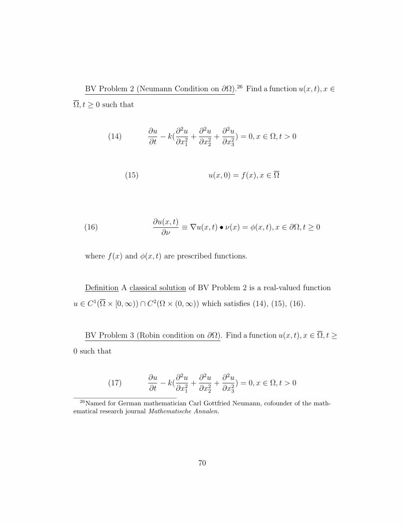
BV Problem 2 (Neumann Condition on ∂Ω).26 Find a function u(x, t), x ∈
Ω, t ≥ 0 such that
(14)∂u
∂t− k(
∂2u
∂x21
+∂2u
∂x22
+∂2u
∂x23
) = 0, x ∈ Ω, t > 0
(15) u(x, 0) = f(x), x ∈ Ω
(16)∂u(x, t)
∂ν≡ ∇u(x, t) • ν(x) = φ(x, t), x ∈ ∂Ω, t ≥ 0
where f(x) and φ(x, t) are prescribed functions.
Definition A classical solution of BV Problem 2 is a real-valued function
u ∈ C1(Ω× [0,∞)) ∩ C2(Ω× (0,∞)) which satisfies (14), (15), (16).
BV Problem 3 (Robin condition on ∂Ω). Find a function u(x, t), x ∈ Ω, t ≥
0 such that
(17)∂u
∂t− k(
∂2u
∂x21
+∂2u
∂x22
+∂2u
∂x23
) = 0, x ∈ Ω, t > 0
26Named for German mathematician Carl Gottfried Neumann, cofounder of the math-ematical research journal Mathematische Annalen.
70
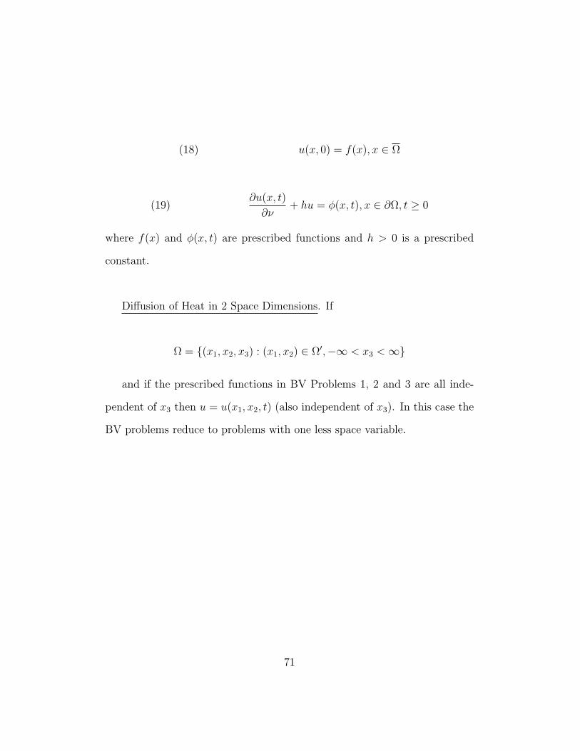
(18) u(x, 0) = f(x), x ∈ Ω
(19)∂u(x, t)
∂ν+ hu = φ(x, t), x ∈ ∂Ω, t ≥ 0
where f(x) and φ(x, t) are prescribed functions and h > 0 is a prescribed
constant.
Diffusion of Heat in 2 Space Dimensions. If
Ω = (x1, x2, x3) : (x1, x2) ∈ Ω′,−∞ < x3 <∞
and if the prescribed functions in BV Problems 1, 2 and 3 are all inde-
pendent of x3 then u = u(x1, x2, t) (also independent of x3). In this case the
BV problems reduce to problems with one less space variable.
71
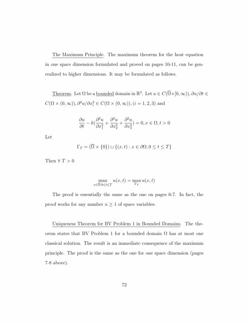
The Maximum Principle. The maximum theorem for the heat equation
in one space dimension formulated and proved on pages 10-11, can be gen-
eralized to higher dimensions. It may be formulated as follows.
Theorem. Let Ω be a bounded domain in R3. Let u ∈ C(Ω×[0,∞)), ∂u/∂t ∈
C(Ω× (0,∞)), ∂2u/∂x2i ∈ C(Ω× (0,∞)), (i = 1, 2, 3) and
∂u
∂t− k(
∂2u
∂x21
+∂2u
∂x22
+∂2u
∂x23
) = 0, x ∈ Ω, t > 0
Let
ΓT = (Ω× 0) ∪ (x, t) : x ∈ ∂Ω, 0 ≤ t ≤ T
Then ∀ T > 0
maxx∈Ω,0≤t≤T
u(x, t) = maxΓT
u(x, t)
The proof is essentially the same as the one on pages 6-7. In fact, the
proof works for any number n ≥ 1 of space variables.
Uniqueness Theorem for BV Problem 1 in Bounded Domains. The the-
orem states that BV Problem 1 for a bounded domain Ω has at most one
classical solution. The result is an immediate consequence of the maximum
principle. The proof is the same as the one for one space dimension (pages
7-8 above).
72
Uniqueness Theorems for BV Problems 2 and 3 in Bounded Domains. In
the case of BV Problems 2 and 3 the uniqueness of classical solutions does
not follow immediately from the maximum principle as it does for BV Prob-
lem 1. Another method of proving uniqueness will now be given that works
for these two problems. The following notation will be used in the proof.
∇u = (∂u
∂x1
,∂u
∂x2
,∂u
∂x3
)
4u = ∇ •∇u =∂2u
∂x21
+∂2u
∂x22
+∂2u
∂x23
Note also the identity
(20) ∇ • (u∇v) = ∇u • ∇v + u4 v
Theorem If Ω ∈ R3 is a bounded domain for which the divergence theorem
holds (this is a type of restriction on ∂Ω) then BV problems 2 and 3 have at
most one classical solution.
Proof. Note that BV problem 3 with h = 0 is the same as BV problem
2. Hence it will be enough to discuss BV problem 3 with condition h ≥ 0.
To prove that at most one classical solution exists we suppose that u1(x, t)
and u2(x, t) are any two classical solutions with the same “data” f(x), φ(x, t)
and consider the difference
73
u(x, t) = u1(x, t)− u2(x, t)
By linearity, u(x, t) is a classical solution of BV problem 3 with data
f(x) ≡ 0 in Ω, φ(x, t) ≡ 0 on ∂Ω× [0,∞). Now consider the function
J(t) =
∫Ω
u(x, t)2dx, t ≥ 0
J(t) is finite ∀ t ≥ 0 because Ω is bounded and u(., t) ∈ C(Ω),∀ t ≥ 0.
Moreover, it is easy to verify that
J(t) ∈ C[0,∞) ∩ C1(0,∞)
and
J ′(t) = 2
∫Ω
u(x, t)∂u(x, t)
∂tdx, t ≥ 0
Using the heat equation for u gives
J ′(t) = 2
∫Ω
u(x, t)4 u(x, t)dx
Combining this with (20), with v = u, gives
J ′(t) = 2
∫Ω
∇ • (u∇u)dx− 2
∫Ω
|∇u(x, t)|2dx
Next, using the divergence theorem gives
74
J ′(t) = 2
∫∂Ω
u∇u • ν(x)dS − 2
∫Ω
|∇u|2dx
= 2
∫∂Ω
u∂u
∂νdS − 2
∫Ω
|∇u|2dx
Finally, using (19) with φ(x, t) ≡ 0 gives
J ′(t) = −2h
∫∂Ω
u(x, t)2dS − 2
∫Ω
|∇u(x, t)|2dx ≤ 0, ∀t > 0
because h ≥ 0. Moreover, the initial condition (18) with f(x) ≡ 0 implies
J(0) = 0. Thus we deduce that
(21) J(t) = J(0) +
∫ t
0
J ′(τ)dτ =
∫ t
0
J ′(τ)dτ ≤ 0, ∀ t ≥ 0
But, since u(., t) ∈ C(Ω), ∀ t ≥ 0, (21) implies27 that
u(x, t) = u1(x, t)− u2(x, t) ≡ 0, ∀ x ∈ Ω, t ≥ 0
i.e.,
u1(x, t) = u2(x, t)
QED.
Remark 1. The same method also works for BV problem 1 if the diver-
gence theorem holds for the domain Ω.
27by the definition of J
75
Remark 2. The proof works for any number n ≥ 1 of space dimensions.28
28The divergence theorem for n = 1 dimensions is just the integration by parts formula.
76
Chapter 5.
The Cauchy Problem for the Heat Equation in 1 Space Dimension.
So far, our results for the heat equation have been restricted to bounded do-
mains. The Cauchy problem asks for a function u(x, t) such that
(1)∂u
∂t=∂2u
∂x2for −∞ < x <∞, t > 0
(2) u(x, 0) = uo(x) for −∞ < x <∞
where uo(x) is a prescribed function.
In this chapter the existence, uniqueness and construction of a solution
of (1), (2) is studied. It will be seen that uniqueness holds only if restrictions
are placed on the initial value function uo(x) and the class of solutions u(x, t)
admitted.
It will be helpful to think of the solution of (1), (2) as describing the
temperature distribution in an infinite uniform rod whose surface is insulated.
Thus temperature will satisfy (1) if
(3) k =K
cρ= 1
which also can be achieved by the proper choice of time unit. It will also be
assumed that
77
(4) cρ = 1 (choice of unit of heat)
and
(5) A = 1 (choice of unit of length)
Diffusion of Heat From a Point Source - The Fundamental Solution. Sup-
pose that the infinite uniform rod is at temperature 0 for t < 0 and imagine
that at time t = 0 1 unit of heat is introduced in a section xo ≤ x ≤ xo + ∆x
of the rod. If the heat is distributed uniformly in [xo, xo + ∆x] the result will
be an increase in temperature of the section from 0 to a uniform tempera-
ture To = const. in [xo, xo + ∆x]. By the definition of specific heat and the
assumptions (3), (4), (5)
Net increase in heat content of [xo, xo+∆x] = 1 = c× ρA∆x︸ ︷︷ ︸mass of section
× (To−0) = To∆x
Thus the introduction of unit heat, uniformly distributed in [xo, xo+∆x],
produces an initial temperature distribution
(6) uo(x) = u∆x(x, xo) =
1
∆x, xo ≤ x ≤ xo + ∆x
0 elsewhere
Let u∆x(x, xo, t) denote the subsequent temperature distribution, i.e., the
78
solution of (1), (2) with uo(x) defined by (6) (it is assumed for the moment
to exist).
[See blackboard illustration.]
The total quantity of heat in the infinite rod for any time t, is
(7) Q∆x =
∫ ∞
−∞cρAu∆x(x, xo, t)dx =
∫ ∞
−∞u∆x(x, xo, t)dx
The “conservation of energy” principle implies that this should be inde-
pendent of t. Indeed, this is verified by the following calculation:
Q′∆x(t) =
∫ ∞
−∞
∂u∆x(x, xo, t)
∂tdx =
∫ ∞
−∞
∂2u∆x(x, xo, t)
∂x2dx = 0
provided ∂u∆x(x, xo, t)/∂x → 0 when x → ±∞. This is clearly the case.
Thus
(8) Q∆x(t) = Q∆x(o+) = 1, ∀ t > 0
The Limiting Case of a Point Source. Now make ∆x → 0 and assume,
tentatively, that the limit
(9) φ(x, xo, t) = lim∆x→0
u∆x(x, xo, t)
79
exists. This will be verified below. The limiting function φ(x, xo, t) should
describe the temperature distribution at time t > 0 due to a unit amount of
heat released at the point xo at time t = 0.
Intuitively, this corresponds to the Cauchy problem (1), (2) with the
initial distribution
uo(x) = δ(x− xo) (Dirac δ-function)
but use of distribution theory will be avoided here. The limit function (9)
may be expected to have the following properties
(10)∂φ
∂t=∂2φ
∂x2∀ x, xo ∈ R and t > 0
(11) limt→0+
φ(x, xo, t) = 0 ∀ x 6= xo
(12)
∫ ∞
−∞φ(x, xo, t)dx = 1 ∀ xo, t > 0
(13) φ(x, xo, t) ≥ 0, ∀x, xo ∈ R, t > 0
A function φ(x, xo, t) having these properties will now be constructed. As
a working hypothesis, it will be assumed that there is exactly one function
having properties (10)-(13). This assumption will be shown to lead to a
construction of φ(x, xo, t). The latter is part of folklore in PDEs, summarized
80
by phrase, “uniqueness implies existence.”
Step 1. Let φ(x, xo, t) be the function having properties (10)-(13) and
consider the function φ′(x, xo, t) defined by
(14) φ′(x, xo, t) = φ(x− ξ, xo − ξ, t), ξ ∈ R
It is clear that for each fixed ξ ∈ R φ′ also satisfies (10)-(13). Hence, by
the assumed uniqueness of φ
(15) φ(x, xo, t) = φ(x− ξ, xo − ξ, t) ∀ x, xo, ξ ∈ R, t > 0
Taking xo = ξ in (14) gives
(16) φ(x, xo, t) = φ(x− xo, t) ∀ x, xo ∈ R, t > 0
where φ(x, t) is the function defined by
(17) φ(x, t) = φ(x, 0, t)
Thus φ(x, t) satisfies
(18)∂φ(x, t)
∂t=∂2φ(x, t)
∂x2∀ x ∈ R and t > 0
81
(19) limt→0+
φ(x, t) = 0 ∀ x 6= 0
(20)
∫ ∞
−∞φ(x, t)dx = 1 ∀ t > 0
(21) φ(x, t) ≥ 0, ∀x ∈ R, t > 0
Step 2. Consider the function
(22) φ′(x, t) = αnφ(αx, α2t), α > 0
For any fixed α > 0 it satisfies (18), (19) and (21). Moreover,
∫ ∞
−∞φ′(x, t)dx = αn
∫ ∞
−∞φ(αx, α2t)dx = αn−1
∫ ∞
−∞φ(y, α2y)dy = 1
if and only if αn−1 = 1; i.e., α = 1 or n = 1. Thus αφ(α(x−xo), α2t) has the
properties (10)-(13) for any α > 0 and hence by the assumed uniqueness
(23) φ(x, t) = φ(x, 0, t) = αφ(αx, α2t) ∀ α > 0
Taking α = t−12 gives
(24) φ(x, t) = t−12φ(t−
12x)
82
where φ(x) is the function of x ∈ R defined by
(25) φ(ξ) = φ(ξ, 1), ξ ∈ R
To find the properties of φ(ξ) corresponding to (18)-(21) note that differ-
entiating (24) gives
∂φ(x, t)
∂t= −1
2t−
32φ(
x
t12
)− 1
2t−
12 t−
32xφ′(
x
t12
) = −1
2t
32 (φ(ξ) + ξφ′(ξ))
where
ξ =x
t12
Similarly,
∂φ(x, t)
∂x=
1
tφ′(
x
t12
),∂2φ
∂x2=
1
t32
φ′′(ξ)
Whence,
∂2φ(x, t)
∂x2− ∂φ(x, t)
∂t=
1
t32
φ′′(ξ) +ξ
2φ′(ξ) +
1
2φ(ξ) = 0
Also,
∫ ∞
−∞φ(x, t)dx = t
12
∫ ∞
−∞φ(t−
12x)dx =
∫ ∞
−∞φ(ξ)dξ = 1
and
83
limt→0+
φ(x, t) = limt→0+
1
x
x
t12
φ(x
t12
) =1
xlim
ξ→±∞ξφ(ξ) = 0
for all x 6= 0 (x > 0⇔ ξ →∞, x < 0⇔ ξ → −∞.)
Thus (24) has properties (18) - (21) if and only if φ(ξ) satisfies the con-
ditions
(26)d2φ
dξ2+ξ
2
dφ
dξ+
1
2φ = 0 ∀ ξ ∈ R
(27) limt→±∞
ξφ(ξ) = 0
(28)
∫ ∞
−∞φ(ξ)dξ = 1
(29) φ(ξ) ≥ 0 ∀ ξ ∈ R
It will be shown that (26)-(28) determine φ(ξ) uniquely.
Step 3. To integrate (26) note that
d
dξ(dφ
dξ+ξ
2φ) ≡ d2φ
dξ2+ξ
2
dφ
dξ+
1
2φ
Thus (26) is equivalent to the 1st order equation
(30)dφ
dξ+ξ
2φ = K = const. ξ ∈ R
If K = 0 then separation of variables gives
84
φ = ce−ξ24
where c is any constant. The method of variation of constants29 then gives
the general solution
(31) ce−ξ2/4 + c′e−ξ
2/4
∫ ξ
0
eτ2/4dτ
where c and c′ are arbitrary constants. To determine them, conditions (27)-
(29) will be used. Note that, by repeated use of l’Hopital’s rule
limξ→±∞
ξe−ξ2/4
∫ ξ
0
eτ2/4dτ = lim
ξ→±∞
ξ∫ ξ
0eτ
2/4dτ
eξ2/4
= limξ→±∞
∫ ξ
0eτ
2/4dτ + ξeξ2/4
12ξeξ2/4
= 2 + limξ→±∞
eξ2/4
12ξeξ2/4 + ξ2
4eξ2/4
= 2
Thus (31) will satisfy (27) if and only if c′ = 0. Thus
(32) φ(ξ) = ce−ξ2/4
To find c we have, by (28)
29Also called variation of parameters.
85
∫ ∞
−∞φ(ξ)dξ = c
∫ ∞
−∞eξ
2/4dξ = c(4π)1/2 = 1
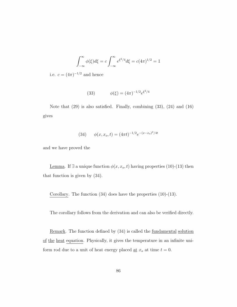
i.e. c = (4π)−1/2 and hence
(33) φ(ξ) = (4π)−1/2eξ2/4
Note that (29) is also satisfied. Finally, combining (33), (24) and (16)
gives
(34) φ(x, xo, t) = (4πt)−1/2e−(x−xo)2/4t
and we have proved the
Lemma. If ∃ a unique function φ(x, xo, t) having properties (10)-(13) then
that function is given by (34).
Corollary. The function (34) does have the properties (10)-(13).
The corollary follows from the derivation and can also be verified directly.
Remark. The function defined by (34) is called the fundamental solution
of the heat equation. Physically, it gives the temperature in an infinite uni-
form rod due to a unit of heat energy placed at xo at time t = 0.
86
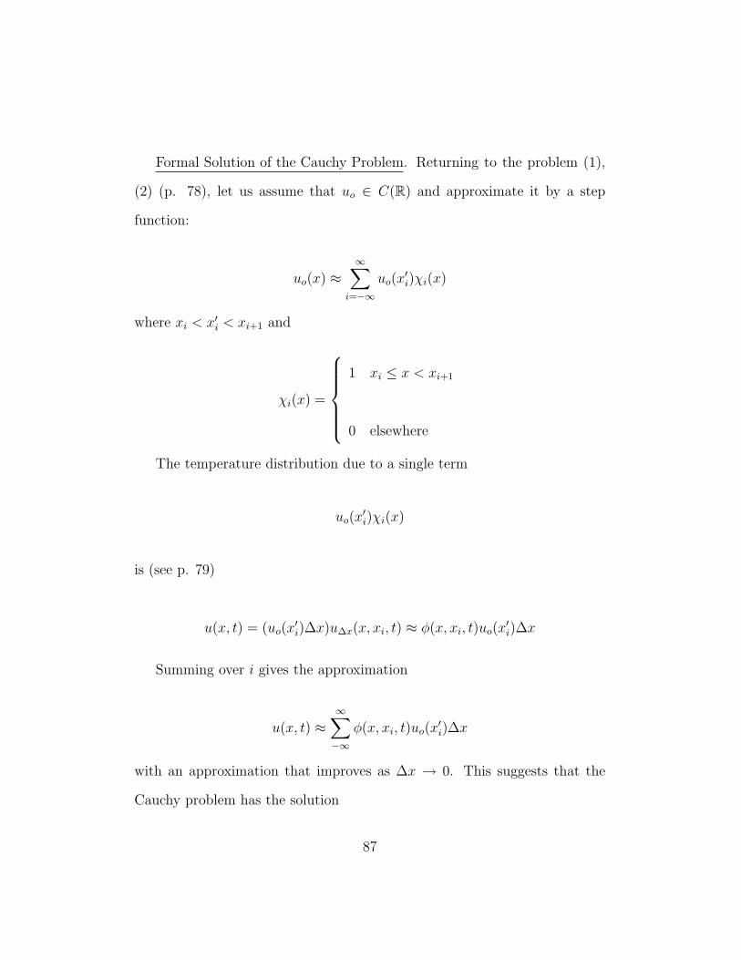
Formal Solution of the Cauchy Problem. Returning to the problem (1),
(2) (p. 78), let us assume that uo ∈ C(R) and approximate it by a step
function:
uo(x) ≈∞∑
i=−∞
uo(x′i)χi(x)
where xi < x′i < xi+1 and
χi(x) =
1 xi ≤ x < xi+1
0 elsewhere
The temperature distribution due to a single term
uo(x′i)χi(x)
is (see p. 79)
u(x, t) = (uo(x′i)∆x)u∆x(x, xi, t) ≈ φ(x, xi, t)uo(x
′i)∆x
Summing over i gives the approximation
u(x, t) ≈∞∑−∞
φ(x, xi, t)uo(x′i)∆x
with an approximation that improves as ∆x → 0. This suggests that the
Cauchy problem has the solution
87
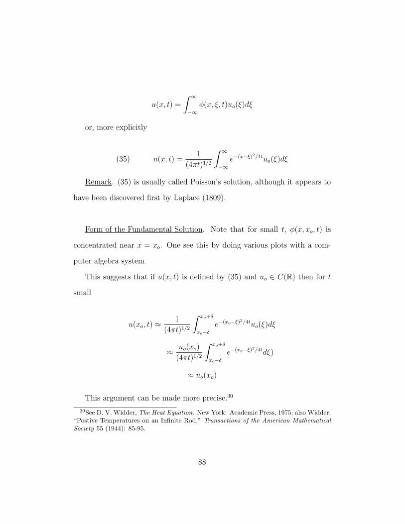
u(x, t) =
∫ ∞
−∞φ(x, ξ, t)uo(ξ)dξ
or, more explicitly
(35) u(x, t) =1
(4πt)1/2
∫ ∞
−∞e−(x−ξ)2/4tuo(ξ)dξ
Remark. (35) is usually called Poisson’s solution, although it appears to
have been discovered first by Laplace (1809).
Form of the Fundamental Solution. Note that for small t, φ(x, xo, t) is
concentrated near x = xo. One see this by doing various plots with a com-
puter algebra system.
This suggests that if u(x, t) is defined by (35) and uo ∈ C(R) then for t
small
u(xo, t) ≈1
(4πt)1/2
∫ xo+δ
xo−δe−(xo−ξ)2/4tuo(ξ)dξ
≈ uo(xo)
(4πt)1/2
∫ xo+δ
xo−δe−(xo−ξ)2/4tdξ)
≈ uo(xo)
This argument can be made more precise.30
30See D. V. Widder, The Heat Equation. New York: Academic Press, 1975; also Widder,“Postive Temperatures on an Infinite Rod.” Transactions of the American MathematicalSociety 55 (1944): 85-95.
88
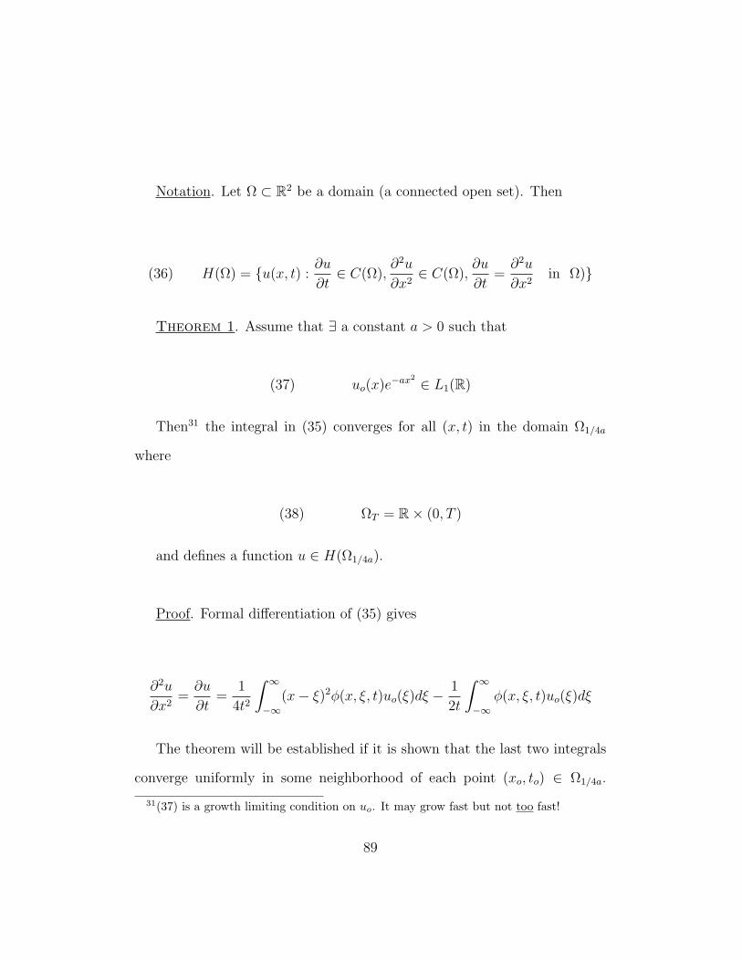
Notation. Let Ω ⊂ R2 be a domain (a connected open set). Then
(36) H(Ω) = u(x, t) :∂u
∂t∈ C(Ω),
∂2u
∂x2∈ C(Ω),
∂u
∂t=∂2u
∂x2in Ω)
Theorem 1. Assume that ∃ a constant a > 0 such that
(37) uo(x)e−ax2 ∈ L1(R)
Then31 the integral in (35) converges for all (x, t) in the domain Ω1/4a
where
(38) ΩT = R× (0, T )
and defines a function u ∈ H(Ω1/4a).
Proof. Formal differentiation of (35) gives
∂2u
∂x2=∂u
∂t=
1
4t2
∫ ∞
−∞(x− ξ)2φ(x, ξ, t)uo(ξ)dξ −
1
2t
∫ ∞
−∞φ(x, ξ, t)uo(ξ)dξ
The theorem will be established if it is shown that the last two integrals
converge uniformly in some neighborhood of each point (xo, to) ∈ Ω1/4a.
31(37) is a growth limiting condition on uo. It may grow fast but not too fast!
89
Choose δ > 0 such that
N(xo, to) = (x, t) : |x− xo| < δ, |t− to| < δ ⊂ Ω1/4a
It will be shown that the integrals are dominated by convergent integrals
whose integrands are independent of (x, t) ∈ N(xo, to). Consider first the
two integrals restricted over the partial range [R,∞) where R > xo + δ. We
have for xo − δ < x < xo + δ, ξ ≥ R, 0 < to − δ < t < to + δ < t/4a
φ(x, ξ, t) =1
(4πt)1/2e−(x−ξ)2/4t ≤ 1
(4πt)1/2e−(ξ−xo−δ)2/4t
≤ 1
(4πt)1/2e−(x−ξ)2/4(to+δ) ≤ 1
4π(to − δ))1/2e−(ξ−xo−δ)2/4(to+δ)
= Cφ(xo + δ, ξ, to + δ)
where
C =
√to + δ
to − δ
Similarly, ∀ (x, t) ∈ N(xo, to) and R ≤ ξ <∞
(x− ξ)2φ(x, ξ, t) ≤ C(ξ − xo + δ)2φ(xo + δ, ξ, to + δ)
Since to + δ < 1/4a it follows that
φ(xo + δ, ξ, to + δ)eaξ2 ≤ K1 ∀ ξ ∈ [R,∞)
90
(ξ − xo + δ)2φ(xo + δ, ξ, to + δ)eaξ2 ≤ K2 ∀ ξ ∈ [R,∞)
Then
|φ(x, ξ, t)uo(ξ)| ∈ CK1|uo(ξ)e−aξ2| ∈ L1([R,∞))
for all (x, t) ∈ N(xo, to). The remaining integrals can be treated in the same
way. QED.
Theorem 2. Assume that uo satisfies (37) and that the limits uo(xo+)
and uo(xo−) exist. Then the function u ∈ H(Ω1/4a) defined by (35) satisfies32
(39) lim supx→xo,t→0+
|u(x, t)| ≤ max(|uo(xo+)|, |uo(xo−)|)
If in addition, uo(x+) = uo(xo−) then
(40) limx→xo,t→0+
u(x, t) = uo(xo+)
Remark. The notation x→ xo, t→ 0 means that (x, t)→ (xo, 0) through
points of the half plane t > 0. The approach is otherwise unrestricted.
Proof of Theorem 2. Let M = max(|uo(xo+)|, |uo(xo−)|). Then ∀ ε >
0 ∃ δ > 0 such that
(41) |uo(ξ)| < M + ε for |ξ − xo| ≤ δ
32See Appendix IV.
91
Thus if
u(x, t) =
∫ xo−δ
−∞φ(x, ξ, t)uo(ξ)dξ+
∫ xo+δ
xo−δφ(x, ξ, t)uo(ξ)dξ+
∫ ∞
xo+δ
φ(x, ξ, t)uo(ξ)dξ
= I1 + I2 + I3
then
|I2| ≤ (M + ε)
∫ ∞
−∞φ(x, ξ, t)uo(ξ)dξ = M + ε, ∀ x ∈ R, t > 0.
Moreover, if |x−xo| < ρ < δ, ξ ≥ xo+δ then −xo−ρ < x < xo+ρ, ξ−x ≥
ξ − xo − ρ and hence
φ(x, ξ, t) ≤ 1
(4πt)1/2e−(ξ−xo−ρ)/4t = φ(xo + ρ, ξ, t)
Thus if |x− xo| < ρ then
|I3| ≤∫ ∞
xo+δ
φ(xo + ρ, ξ, t)|uo(ξ)|dξ
Now
φ(xo + ρ, ξ, t)eaξ2
is a decreasing function of ξ for ξ ≥ xo + δ and all t sufficiently small. (In
fact it has its maximum at ξ = (xo + ρ)/(1− 4at).) Thus
92
φ(xo + ρ, ξ, t)eaξ2 ≤ φ(xo + ρ, xo + δ, t)ea(xo+δ)2 , ξ ≥ xo + δ
or
φ(xo + ρ, ξ, t) ≤ [φ(ρ, δ, t)ea(xo+δ)2 ]e−aξ2
, ξ ≥ xo + δ
and
|I3| ≤ [φ(ρ, δ, t)ea(xo+δ)2 ]
∫ ∞
xo+δ
e−aξ2 |uo(ξ)dξ
∀ (x, t) with |x− xo| < ρ, t > 0. Making t→ 0+ gives
lim supx→xo,t→0+
|I3(x, t)| = 0
The integral I1 has the same property. Thus by (42)
lim supx→xo,t→0+
|u(x, t)| ≤M + ε, ∀ ε > 0
which implies (39). To prove (40), write
u(x, t)− uo(xo+) =
∫ ∞
−∞φ(x, ξ, t)[uo(ξ)− uo(xo+)]dξ = I ′1 + I ′2 + I ′3
as above. Following the same reasoning as above,
93
|I ′2(x, t)| ≤ sup|x−xo|≤δ
|uo(ξ)− uo(xo+)|+ ε
and the argument used above gives
lim supx→xo,t→0+
|u(x, t)− uo(xo+)| ≤ sup|ξ−xo|≤δ
|uo(ξ)− uo(xo+)|, ∀ δ > 0
If uo(xo−) = uo(xo+) the last expression tends to zero with δ which
proves (40). QED.
Theorems 1 and 2 can be combined to give an existence theorem for the
Cauchy problem. The notation ΩT as above and
ΩT = R× [0, T )
will be used.
Definition. A classical solution of the Cauchy problem (1), (2) (p. 78) in
a domain ΩT is a function
u ∈ H(ΩT ) ∩ C(ΩT )
such that u(x, 0) = uo(x) for all x ∈ R.
Observe that uo ∈ C(R) is a necessary condition for the existence of a
classical solution. Theorems 1 and 2 imply that continuity and condition
(37) are sufficient. More precisely, the following theorem holds.
94
Existence Theorem. Assume that
(a) uo ∈ C(R)
(b) ∃ a > 0 such that uo(x)e−ax2 ∈ L1(R)
Then the integral (35) defines a classical solution of the Cauchy problem
in the domain Ω1/4a.
Proof. Theorems 1 and 2 imply that u ∈ H(Ω1/4a) and that
limx→xo,t→0+
u(x, t) = uo(xo)
for all xo. This property and the continuity of uo imply that u ∈ C(Ω1/4a)
and u(x, 0) = uo(x), ∀ x ∈ R. QED.
Corollary. Assume that
(a) uo ∈ C(R)
(b) ∃M such that |uo(x)| ≤M, ∀ x ∈ R
Then (35) defines a classical solution of the Cauchy problem in Ω∞ = R2+.
Moreover
|u(x, t)| ≤M ∀ (x, t) ∈ R2+
.
Proof. The boundedness condition (b) implies that condition (b) of the
95
Existence Theorem holds for all a > 0. (35) implies the second part of the
corollary. QED.
————
The heat equation is strongly linked to the notion of absolute zero. In
fact it is possible to show that:
Widder’s Representation Theorem. A real-valued function u(x, t) has the
properties
(1) u ∈ H(ΩT )
(2) u(x, t) ≥ 0, ∀ (x, t) ∈ ΩT
if and only if there exists a real non-decreasing function α(x) defined on
R such that
(3) u(x, t) =
∫ ∞
−∞φ(x, ξ, t)dα(ξ) ∀ (x, t) ∈ ΩT
The class of solutions defined by (3) is more general than that defined by
Poisson’s integral with locally integrable uo(x). However we will not prove
this theorem since it requires some elementary measure theory.
96
Chapter 6. Steady Temperature in a Finite Cylinder.
In Chapter 3 (p. 32) we considered the case of a long cylinder. We now
consider the case of a finite cylinder. Let Ω be a cylinder of radius a and
length l. Let the x3-axis be the axis of the cylinder with x3 = 0 corresponding
to the base of the cylinder and x3 = l the top. The steady-state temperature
us will satisfy
(1)∂2us∂x2
1
+∂2us∂x2
2
+∂2us∂x2
3
= ∆us = 0, x = (x1, x2, x3) ∈ Ω
(2) us(x1, x2, 0) = f(x1, x2), x21 + x2
2 ≤ a2
(3) us(x1, x2, l) = g(x1, x2), x21 + x2
2 ≤ a2
(4) us(x1, x2, x3) = h(x1, x2, x3), x21 + x2
2 = a2, 0 ≤ x3 ≤ l
(2)-(4) respectively correspond to the prescribed temperature at the bottom,
top and side of Ω. Observe that conditions (2)-(3) suggest the consistency conditions
f(x1, x2) = h(x1, x2, 0), g(x1, x2) = h(x1, x2, l), x21 + x2
2 = a2. The circu-
lar nature of the problem suggests a change of coordinates, (x1, x2, x3) →
(r, θ, x3) which is the familiar cylindrical coordinate transformation.
Put us(x1, x2, x3) = v(r, θ, x3). The calculations on pp. 33-34 show that
v satisfies
97
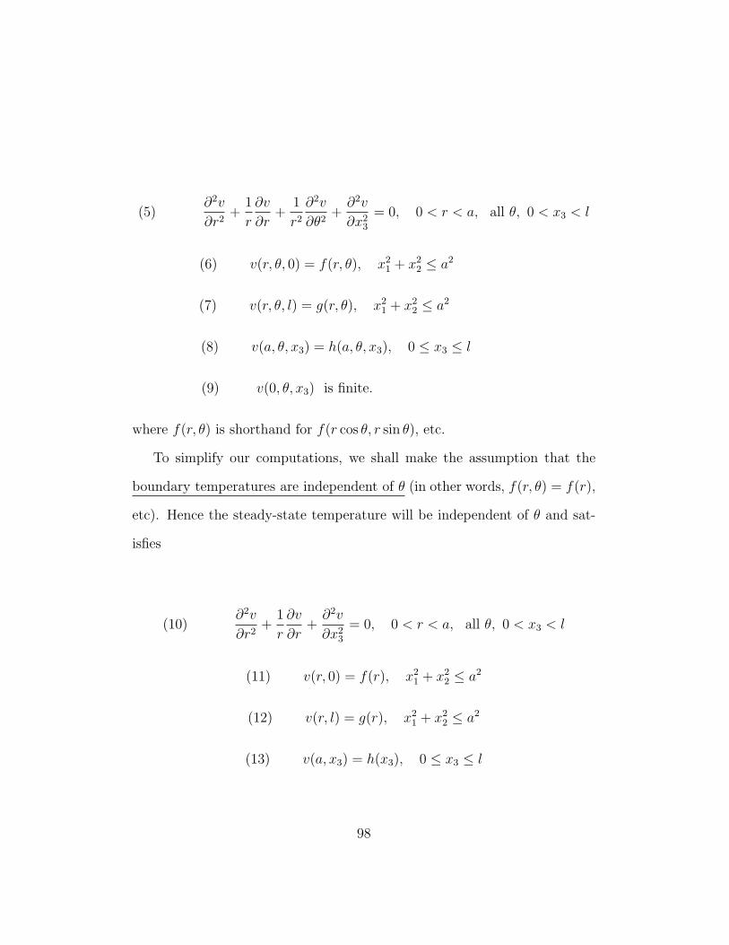
(5)∂2v
∂r2+
1
r
∂v
∂r+
1
r2
∂2v
∂θ2+∂2v
∂x23
= 0, 0 < r < a, all θ, 0 < x3 < l
(6) v(r, θ, 0) = f(r, θ), x21 + x2
2 ≤ a2
(7) v(r, θ, l) = g(r, θ), x21 + x2
2 ≤ a2
(8) v(a, θ, x3) = h(a, θ, x3), 0 ≤ x3 ≤ l
(9) v(0, θ, x3) is finite.
where f(r, θ) is shorthand for f(r cos θ, r sin θ), etc.
To simplify our computations, we shall make the assumption that the
boundary temperatures are independent of θ (in other words, f(r, θ) = f(r),
etc). Hence the steady-state temperature will be independent of θ and sat-
isfies
(10)∂2v
∂r2+
1
r
∂v
∂r+∂2v
∂x23
= 0, 0 < r < a, all θ, 0 < x3 < l
(11) v(r, 0) = f(r), x21 + x2
2 ≤ a2
(12) v(r, l) = g(r), x21 + x2
2 ≤ a2
(13) v(a, x3) = h(x3), 0 ≤ x3 ≤ l
98
(14) v(0, x3) is finite.
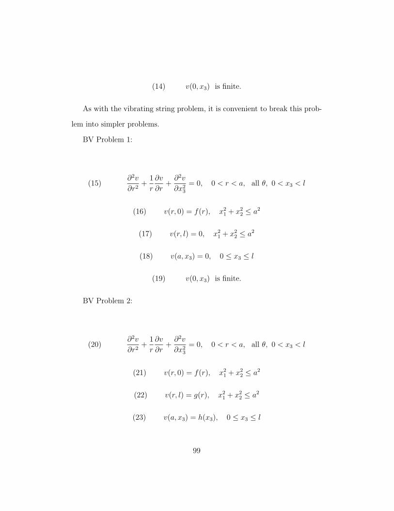
As with the vibrating string problem, it is convenient to break this prob-
lem into simpler problems.
BV Problem 1:
(15)∂2v
∂r2+
1
r
∂v
∂r+∂2v
∂x23
= 0, 0 < r < a, all θ, 0 < x3 < l
(16) v(r, 0) = f(r), x21 + x2
2 ≤ a2
(17) v(r, l) = 0, x21 + x2
2 ≤ a2
(18) v(a, x3) = 0, 0 ≤ x3 ≤ l
(19) v(0, x3) is finite.
BV Problem 2:
(20)∂2v
∂r2+
1
r
∂v
∂r+∂2v
∂x23
= 0, 0 < r < a, all θ, 0 < x3 < l
(21) v(r, 0) = f(r), x21 + x2
2 ≤ a2
(22) v(r, l) = g(r), x21 + x2
2 ≤ a2
(23) v(a, x3) = h(x3), 0 ≤ x3 ≤ l
99
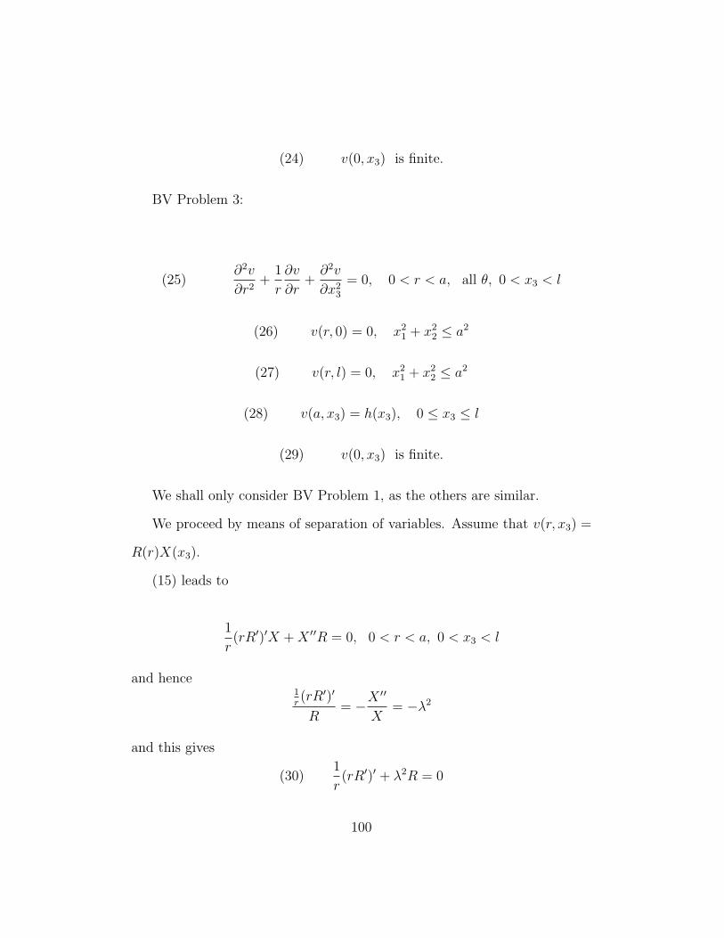
(24) v(0, x3) is finite.
BV Problem 3:
(25)∂2v
∂r2+
1
r
∂v
∂r+∂2v
∂x23
= 0, 0 < r < a, all θ, 0 < x3 < l
(26) v(r, 0) = 0, x21 + x2
2 ≤ a2
(27) v(r, l) = 0, x21 + x2
2 ≤ a2
(28) v(a, x3) = h(x3), 0 ≤ x3 ≤ l
(29) v(0, x3) is finite.
We shall only consider BV Problem 1, as the others are similar.
We proceed by means of separation of variables. Assume that v(r, x3) =
R(r)X(x3).
(15) leads to
1
r(rR′)′X +X ′′R = 0, 0 < r < a, 0 < x3 < l
and hence1r(rR′)′
R= −X
′′
X= −λ2
and this gives
(30)1
r(rR′)′ + λ2R = 0
100
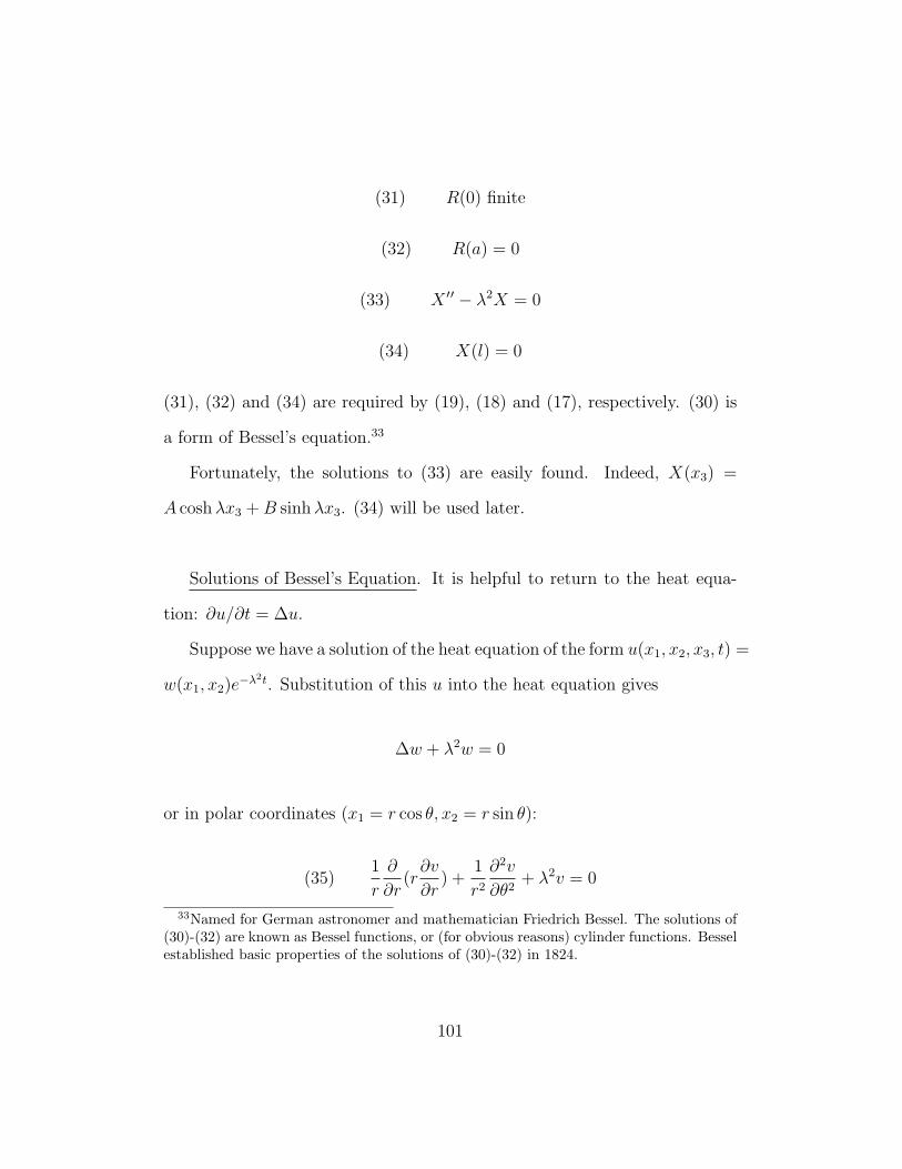
(31) R(0) finite
(32) R(a) = 0
(33) X ′′ − λ2X = 0
(34) X(l) = 0
(31), (32) and (34) are required by (19), (18) and (17), respectively. (30) is
a form of Bessel’s equation.33
Fortunately, the solutions to (33) are easily found. Indeed, X(x3) =
A coshλx3 +B sinhλx3. (34) will be used later.
Solutions of Bessel’s Equation. It is helpful to return to the heat equa-
tion: ∂u/∂t = ∆u.
Suppose we have a solution of the heat equation of the form u(x1, x2, x3, t) =
w(x1, x2)e−λ2t. Substitution of this u into the heat equation gives
∆w + λ2w = 0
or in polar coordinates (x1 = r cos θ, x2 = r sin θ):
(35)1
r
∂
∂r(r∂v
∂r) +
1
r2
∂2v
∂θ2+ λ2v = 0
33Named for German astronomer and mathematician Friedrich Bessel. The solutions of(30)-(32) are known as Bessel functions, or (for obvious reasons) cylinder functions. Besselestablished basic properties of the solutions of (30)-(32) in 1824.
101
(36) v(r, θ + 2π) = v(r, θ)
(37) v(0, θ) finite
Now observe that (30) is a special case of (35) in case v is independent
of θ. Write (35) as
∂2v
∂r2+
1
r
∂v
∂r+
1
r2
∂2v
∂θ2+ λ2v = 0
and integrate with respect to θ:
∫ π
−π
∂2v
∂r2dθ +
1
r
∫ π
−π
∂v
∂rdθ +
1
r2
∫ π
−π
∂2v
∂θ2dθ + λ2
∫ π
−πvdθ = 0
The third integral may be computed and based on (36) is zero. Thus we have
∫ π
−π
∂2v
∂r2dθ +
1
r
∫ π
−π
∂v
∂rdθ + λ2
∫ π
−πvdθ = 0
or
∂2
∂r2
∫ π
−πvdθ +
1
r
∂
∂r
∫ π
−πvdθ + λ2
∫ π
−πvdθ = 0
Thus we may write
(38) R(r) =
∫ π
−πvdθ
Thus every solution of ∆w + λ2w = 0 generates a solution of (30). We
102
may exploit this to obtain information about solutions of (30) which has
no solutions in terms of standard elementary functions. Suppose that w =
eax1+bx2 . Substituting this into ∆w + λ2w = 0 yields a2 + b2 + λ2 = 0. We
may choose a and b in any way, so select a = 0, b = iλ. This gives w = eix2λ.
Introducing polor coordinates again gives
(39) v(r, θ) = eirλ sin θ
Using (38) we have
(40) R(r) =
∫ π
−πeirλ sin θdθ
It is convenient to introduce a normalizing factor into (40):
(41) R(r) =1
2π
∫ π
−πeirλ sin θdθ
This specifies that R(0) = 1. Using Euler’s formula and that sin is an
odd function,
(42) R(r) =1
π
∫ π
0
cos(irλ sin θ)dθ
Now substitution of the Maclaurin series for cosine into (42) gives
R(r) =1
π
∞∑j=0
(−1)j(λr)2j
(2j)!
∫ π
0
sin2j θdθ
103
Reduction formulae can now be used to write
∫ π
0
sin2j θdθ =π(2j)!
22j(j!)2
It follows that R(r) has the power series representation
(43) R(r) =∞∑j=0
(−1)j(λr)2j
j!222j
(43) may be used to obtain approximate values of R(r).
Other forms of R(r) exist and provide other kinds of information. For
example, make the substitution ω = θ − π/2 into (42) which results in
(44) R(r) =2
π
∫ π2
0
cos(λr cosω)dω
Make the substitution t = cosω into (44) to get
(45) R(r) =2
π
∫ 1
0
cos(λrt)√1− t2
dt
The standard notation for R(r) is Jo(rλ). From (42) we observe that
(46) |Jo(rλ)| ≤ 1
For ease of computation, write λ = 1 in (32). (We can always recover R by
104
substituting λr for r.) Then
(47) Jo(r) =2
π
∫ 1
0
cos rt√1− t2
dt
Now change variables again with rt = r − τ . Then (47) becomes
(48) Jo(r) =2
π
∫ r
o
cos(r − τ)√2rτ
√1− τ
2r
dτ
Applying the cosine addition formula we get
(49) Jo(r) =2
π√r
∫ r
o
cos(τ)√2τ
√1− τ
2r
dτ cos r+2
π√r
∫ r
o
sin(τ)√2τ
√1− τ
2r
dτ sin r
As r →∞ ∫ r
o
cos(τ)√2τ
√1− τ
2r
dτ →∫ ∞
o
cos(τ)√2τ
dτ
with a similar result for the sine integral. Both limits can be computed
explicitly, i.e.,
∫ ∞
o
sin(τ)√2τ
dτ =
∫ ∞
o
cos(τ)√2τ
dτ =√π/2
Consequently,
Jo(r) =
√2√πr
[cos(r − π
4) + o(r)] as r →∞
105
Thus Jo(λr) behaves like cos(λr − π/4) for large r. Consequently when
r is large, J will have zeros in each of the intervals [mπλ
+ π4, (m+1)π
λ+ π
4].
Arranging the zeros of Jo(r) as
0 < β1 < β2 < β3...
we see that Jo(r) has properties similar to sine and cosine, although it is not
periodic.
Since (30) is a second order equation, it has two linearly independent
solutions. Of course there are many such pairs. Selecting another solution
in addition to J is partly a matter of usefulness. None of these solutions are
important for our heat conduction problem however: they are all unbounded
at r = 0 which violates (31). However, a common second solution, known as
Weber’s function is given by
Yo(λr) =2
πJo(λr) ln r +
∑ckr
2k
Such solutions become important if we change the geometry of the problem,
for example instead of a finite cylinder, imagine a cylinder with a hole bored
down the center. Then r cannot be zero.
Finishing the Solution to BV Problem 1. The condition R(a) = 0 implies
that λn = βn/a. Hence we have
Rn(r) = Jo(λnr), Xn(x3) = An coshλnx3 +Bn sinhλnx3
106
Recall that X(l) = 0. Hence, An coshλnl +Bn sinhλnl = 0. This implies
that
An = −Bn tanhλnl
and we may define
vn(r, x3) = BnJo(λnr)(− tanhλnl coshλnx3 + sinhλnx3)
Formal Solution. We define
(50) v(r, x3) =∞∑n=1
vn(r, x3), v(r, 0) = f(r)
Then the question of convergence for the series (50) is decided in part by
Fourier-Bessel convergence theory.
Theorem. Let f ′(r) be sectionally continuous on [0, a]. Then for each r,
0 < r < a, the series,
∞∑n=1
AnJo(λnr) =f(r+) + f(r−)
2
converges and the coefficients An are given by
An =2
a2J ′o(βn)
∫ a
0
f(r)Jo(λnr)rdr
We could define the notion of a classical solution and consider an existence
107
theorem in much the same was as we have already done. However, we shall
instead consider a similar problem.
Wave Motion in Two Dimensions.
Le Ω be a circular membrane (e.g., drumhead) of radius a, occupying the
region Ω = (x1, x2) : x21 + x2
2 ≤ a2.
If the membrane or drumhead is under tension, it will vibrate when struck.
For a low-mass drumhead, the transverse displacement from equilibrium u
satisfies the equation
(1)∂2u
∂t2= c2(
∂2u
∂x21
+∂2u
∂x22
), x21 + x2
2 < a2, t > 0
(2) u(x1, x2, 0) = uo(x1, x2), x21 + x2
2 ≤ a2
(3)∂u(x1, x2, 0)
∂t= u1(x1, x2), x2
1 + x22 ≤ a2
(4) u(x1, x2, t) = 0, x21 + x2
2 = a2, t ≥ 0
Conditions (2) and (3) specify the initial shape and velocity of the drum-
head, while condition (4) says that the drum skin is secured at the edge. As
with the vibrating string problem, we make the simplifying assumption that
u1 ≡ 0 (see p. 22). To further simplify our computations, let us assume that
a change of variable has been done to allow us to substitute 1 for c (see p.
13).
Changing to polar coordinates (u(x1, x2, t) = v(r, θ, t)) gives us the prob-
lem
108
(5)∂2v
∂t2=
1
r
∂
∂r(r∂v
∂r) +
1
r2
∂2v
∂θ2, 0 < r < a, t > 0
(6) v(r, θ, 0) = uo(r cos θ, r sin θ) = f(r, θ), ∀ 0 ≤ r ≤ a, θ ∈ R
(7)∂v(r, θ, 0)
∂t= 0, ∀ 0 ≤ r ≤ a, θ ∈ R
(8) v(r, θ, t) = 0, r = a, ∀ t ≥ 0
(9) v(r, θ + 2π, t) = v(r, θ, t), ∀ θ ∈ R, t ≥ 0
(10) v(r, θ, t) finite, r → 0, ∀ θ ∈ R, t ≥ 0
(11) v(a, θ, 0) = 0,∀ θ ∈ R
Separation of Variables.
We perform this in two stages:
Stage 1. Assume v(r, θ, t) = w(r, θ)T (t). Substitution into (5) gives
T ′′w =1
r
∂
∂r(r∂w
∂r)T +
1
r2
∂2w
∂θ2T
or
T ′′
T=
1r∂∂r
(r ∂w∂r
) + 1r2∂2w∂θ2
w= −λ2
Thus
T ′′ + λ2T = 0, T ′(0) = 0 (by (7)
109
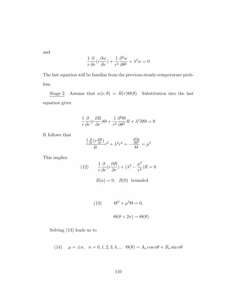
and
1
r
∂
∂r(r∂w
∂r) +
1
r2
∂2w
∂θ2+ λ2w = 0
The last equation will be familiar from the previous steady-temperature prob-
lem.
Stage 2. Assume that w(r, θ) = R(r)Θ(θ). Substitution into the last
equation gives
1
r
∂
∂r(r∂R
∂r)Θ +
1
r2
∂2Θ
∂θ2R + λ2RΘ = 0
It follows that1r∂∂r
(r ∂R∂r
)
Rr2 + λ2r2 = −
∂2Θ∂θ2
Θ= µ2
This implies
(12)1
r
∂
∂r(r∂R
∂r) + (λ2 − µ2
r2)R = 0
R(a) = 0, R(0) bounded
(13) Θ′′ + µ2Θ = 0,
Θ(θ + 2π) = Θ(θ)
Solving (13) leads us to
(14) µ = ±n, n = 0, 1, 2, 3, 4, ... Θ(θ) = An cosnθ +Bn sinnθ
110
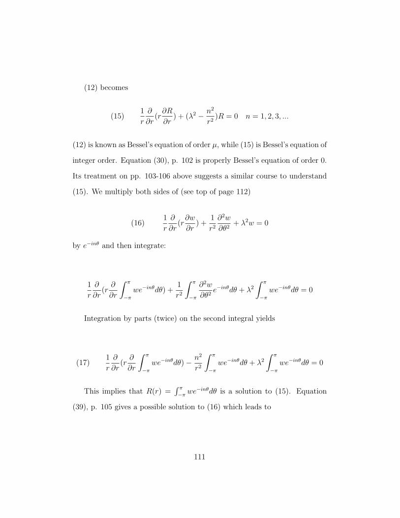
(12) becomes
(15)1
r
∂
∂r(r∂R
∂r) + (λ2 − n2
r2)R = 0 n = 1, 2, 3, ...
(12) is known as Bessel’s equation of order µ, while (15) is Bessel’s equation of
integer order. Equation (30), p. 102 is properly Bessel’s equation of order 0.
Its treatment on pp. 103-106 above suggests a similar course to understand
(15). We multiply both sides of (see top of page 112)
(16)1
r
∂
∂r(r∂w
∂r) +
1
r2
∂2w
∂θ2+ λ2w = 0
by e−inθ and then integrate:
1
r
∂
∂r(r∂
∂r
∫ π
−πwe−inθdθ) +
1
r2
∫ π
−π
∂2w
∂θ2e−inθdθ + λ2
∫ π
−πwe−inθdθ = 0
Integration by parts (twice) on the second integral yields
(17)1
r
∂
∂r(r∂
∂r
∫ π
−πwe−inθdθ)− n2
r2
∫ π
−πwe−inθdθ + λ2
∫ π
−πwe−inθdθ = 0
This implies that R(r) =∫ π
−π we−inθdθ is a solution to (15). Equation
(39), p. 105 gives a possible solution to (16) which leads to
111
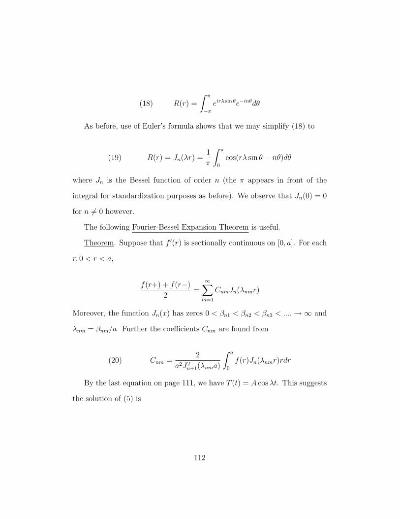
(18) R(r) =
∫ π
−πeirλ sin θe−inθdθ
As before, use of Euler’s formula shows that we may simplify (18) to
(19) R(r) = Jn(λr) =1
π
∫ π
0
cos(rλ sin θ − nθ)dθ
where Jn is the Bessel function of order n (the π appears in front of the
integral for standardization purposes as before). We observe that Jn(0) = 0
for n 6= 0 however.
The following Fourier-Bessel Expansion Theorem is useful.
Theorem. Suppose that f ′(r) is sectionally continuous on [0, a]. For each
r, 0 < r < a,
f(r+) + f(r−)
2=
∞∑m=1
CnmJn(λnmr)
Moreover, the function Jn(x) has zeros 0 < βn1 < βn2 < βn3 < ....→∞ and
λnm = βnm/a. Further the coefficients Cnm are found from
(20) Cnm =2
a2J2n+1(λnma)
∫ a
0
f(r)Jn(λnmr)rdr
By the last equation on page 111, we have T (t) = A cosλt. This suggests
the solution of (5) is
112
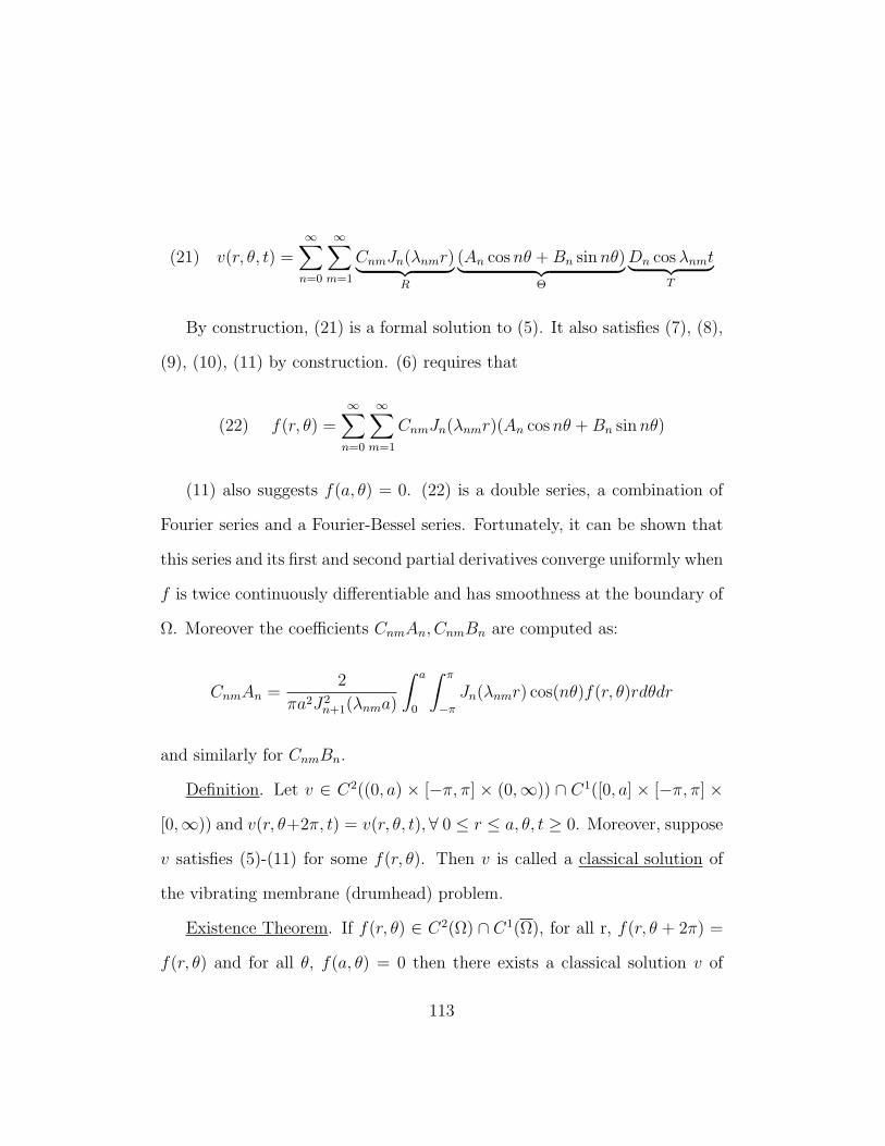
(21) v(r, θ, t) =∞∑n=0
∞∑m=1
CnmJn(λnmr)︸ ︷︷ ︸R
(An cosnθ +Bn sinnθ)︸ ︷︷ ︸Θ
Dn cosλnmt︸ ︷︷ ︸T
By construction, (21) is a formal solution to (5). It also satisfies (7), (8),
(9), (10), (11) by construction. (6) requires that
(22) f(r, θ) =∞∑n=0
∞∑m=1
CnmJn(λnmr)(An cosnθ +Bn sinnθ)
(11) also suggests f(a, θ) = 0. (22) is a double series, a combination of
Fourier series and a Fourier-Bessel series. Fortunately, it can be shown that
this series and its first and second partial derivatives converge uniformly when
f is twice continuously differentiable and has smoothness at the boundary of
Ω. Moreover the coefficients CnmAn, CnmBn are computed as:
CnmAn =2
πa2J2n+1(λnma)
∫ a
0
∫ π
−πJn(λnmr) cos(nθ)f(r, θ)rdθdr
and similarly for CnmBn.
Definition. Let v ∈ C2((0, a) × [−π, π] × (0,∞)) ∩ C1([0, a] × [−π, π] ×
[0,∞)) and v(r, θ+2π, t) = v(r, θ, t),∀ 0 ≤ r ≤ a, θ, t ≥ 0. Moreover, suppose
v satisfies (5)-(11) for some f(r, θ). Then v is called a classical solution of
the vibrating membrane (drumhead) problem.
Existence Theorem. If f(r, θ) ∈ C2(Ω) ∩ C1(Ω), for all r, f(r, θ + 2π) =
f(r, θ) and for all θ, f(a, θ) = 0 then there exists a classical solution v of
113
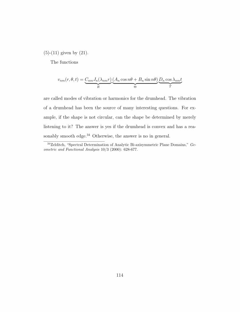
(5)-(11) given by (21).
The functions
vnm(r, θ, t) = CnmJn(λnmr)︸ ︷︷ ︸R
(An cosnθ +Bn sinnθ)︸ ︷︷ ︸Θ
Dn cosλnmt︸ ︷︷ ︸T
are called modes of vibration or harmonics for the drumhead. The vibration
of a drumhead has been the source of many interesting questions. For ex-
ample, if the shape is not circular, can the shape be determined by merely
listening to it? The answer is yes if the drumhead is convex and has a rea-
sonably smooth edge.34 Otherwise, the answer is no in general.
34Zelditch, “Spectral Determination of Analytic Bi-axisymmetric Plane Domains,” Ge-ometric and Functional Analysis 10/3 (2000): 628-677.
114
Chapter 7. The Propagation of Electromagnetic
Waves and The Fourier Transform.
115
Appendix I: Classification of PDEs35
PDEs can be classified in different ways. Some of these are (A) geomet-
ric form, (B) historical significance, (C) associated persons, (D) “algebraic”
form.
As an example of (A) consider an equation of the type
α∂2u
∂x2+ β
∂2u
∂x∂y+ γ
∂2u
∂y2+ δ
∂u
∂x+ ε
∂u
∂y= F (x, y) (1)
This equation is classified as “2nd order” because the highest order derivative
is 2. The values of the coefficients may be used to give a further useful
classification. This is based on obvious correspondence to the equation
αx2 + βxy + γy2 + δx+ εy = F (2)
Geometrically, this equation describes one of the conic sections: ellipse, hy-
perbola, parabola, line. Which one depends on the relative value of the co-
efficients. The equation (1) is classified according as equation (2) is: elliptic,
hyperbolic, parabolic. For example,
y − x2 = 0 (3)
35The perusal of any university library will reveal many monographs and research articleson equations of various types. The survey of types of equations below is by no meansexhaustive.
116
is a parabola. Hence
∂u
∂y− ∂2u
∂x2= 0 (4)
is classified as parabolic. We see that the heat equation is parabolic, while
the wave equation (vibrating string) is hyperbolic.
It is possible for an equation to change its geometric classification if its
coefficients are variable. A simple example is the Tricomi equation:
∂2u
∂x2= x
∂2u
∂y2
This equation is elliptic where x < 0 and hyperbolic when x > 0.
Another important classification is delivered by considering the algebraic
form (D) of the equation rather than the geometric form. For example,
u∂u
∂x− ∂3u
∂y3= x (5)
The first term, u∂u/∂x, is identified as “nonlinear.”36 The reason for this is
that the form does not distribute over sums and constant multiples.
4∂3u
∂z3(6)
is linear since
36Nonlinear equations often present unique challenges and require customized techiquesto study their solutions and properties.
117
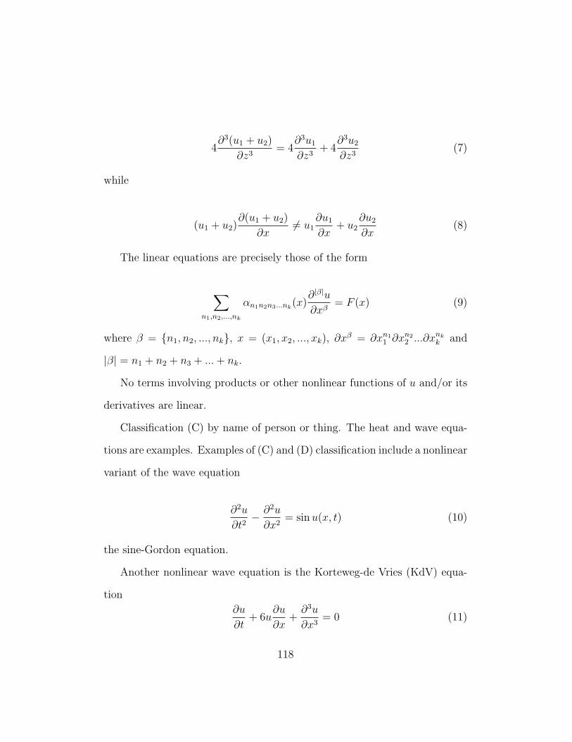
4∂3(u1 + u2)
∂z3= 4
∂3u1
∂z3+ 4
∂3u2
∂z3(7)
while
(u1 + u2)∂(u1 + u2)
∂x6= u1
∂u1
∂x+ u2
∂u2
∂x(8)
The linear equations are precisely those of the form
∑n1,n2,...,nk
αn1n2n3...nk(x)∂|β|u
∂xβ= F (x) (9)
where β = n1, n2, ..., nk, x = (x1, x2, ..., xk), ∂xβ = ∂xn1
1 ∂xn22 ...∂x
nkk and
|β| = n1 + n2 + n3 + ...+ nk.
No terms involving products or other nonlinear functions of u and/or its
derivatives are linear.
Classification (C) by name of person or thing. The heat and wave equa-
tions are examples. Examples of (C) and (D) classification include a nonlinear
variant of the wave equation
∂2u
∂t2− ∂2u
∂x2= sinu(x, t) (10)
the sine-Gordon equation.
Another nonlinear wave equation is the Korteweg-de Vries (KdV) equa-
tion
∂u
∂t+ 6u
∂u
∂x+∂3u
∂x3= 0 (11)
118
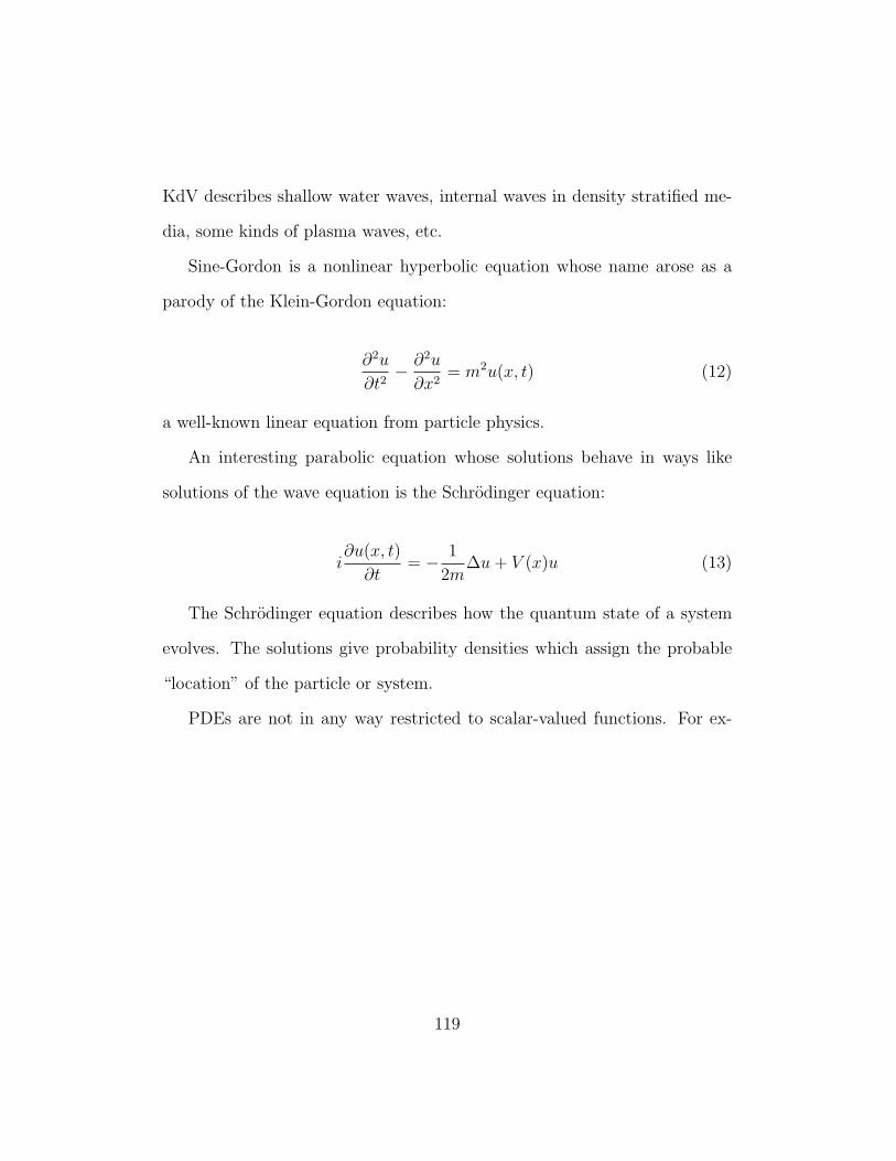
KdV describes shallow water waves, internal waves in density stratified me-
dia, some kinds of plasma waves, etc.
Sine-Gordon is a nonlinear hyperbolic equation whose name arose as a
parody of the Klein-Gordon equation:
∂2u
∂t2− ∂2u
∂x2= m2u(x, t) (12)
a well-known linear equation from particle physics.
An interesting parabolic equation whose solutions behave in ways like
solutions of the wave equation is the Schrodinger equation:
i∂u(x, t)
∂t= − 1
2m∆u+ V (x)u (13)
The Schrodinger equation describes how the quantum state of a system
evolves. The solutions give probability densities which assign the probable
“location” of the particle or system.
PDEs are not in any way restricted to scalar-valued functions. For ex-
119
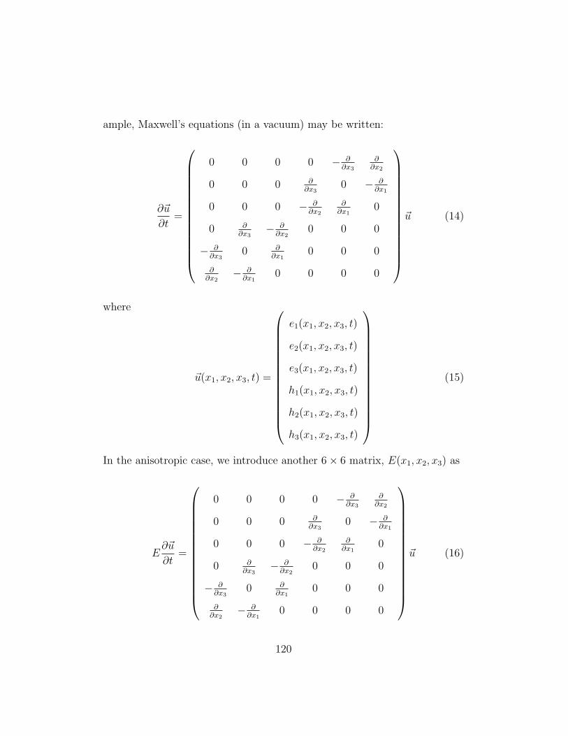
ample, Maxwell’s equations (in a vacuum) may be written:
∂~u
∂t=
0 0 0 0 − ∂∂x3
∂∂x2
0 0 0 ∂∂x3
0 − ∂∂x1
0 0 0 − ∂∂x2
∂∂x1
0
0 ∂∂x3
− ∂∂x2
0 0 0
− ∂∂x3
0 ∂∂x1
0 0 0
∂∂x2
− ∂∂x1
0 0 0 0
~u (14)
where
~u(x1, x2, x3, t) =
e1(x1, x2, x3, t)
e2(x1, x2, x3, t)
e3(x1, x2, x3, t)
h1(x1, x2, x3, t)
h2(x1, x2, x3, t)
h3(x1, x2, x3, t)
(15)
In the anisotropic case, we introduce another 6× 6 matrix, E(x1, x2, x3) as
E∂~u
∂t=
0 0 0 0 − ∂∂x3
∂∂x2
0 0 0 ∂∂x3
0 − ∂∂x1
0 0 0 − ∂∂x2
∂∂x1
0
0 ∂∂x3
− ∂∂x2
0 0 0
− ∂∂x3
0 ∂∂x1
0 0 0
∂∂x2
− ∂∂x1
0 0 0 0
~u (16)
120
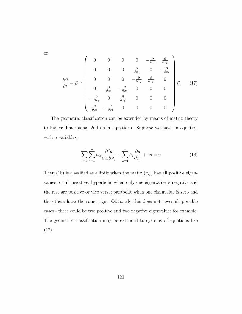
or
∂~u
∂t= E−1
0 0 0 0 − ∂∂x3
∂∂x2
0 0 0 ∂∂x3
0 − ∂∂x1
0 0 0 − ∂∂x2
∂∂x1
0
0 ∂∂x3
− ∂∂x2
0 0 0
− ∂∂x3
0 ∂∂x1
0 0 0
∂∂x2
− ∂∂x1
0 0 0 0
~u (17)
The geometric classification can be extended by means of matrix theory
to higher dimensional 2nd order equations. Suppose we have an equation
with n variables:
n∑i=1
n∑j=1
aij∂2u
∂xi∂xj+
n∑k=1
bk∂u
∂xk+ cu = 0 (18)
Then (18) is classified as elliptic when the matix (aij) has all positive eigen-
values, or all negative; hyperbolic when only one eigenvalue is negative and
the rest are positive or vice versa; parabolic when one eigenvalue is zero and
the others have the same sign. Obviously this does not cover all possible
cases - there could be two positive and two negative eigenvalues for example.
The geometric classification may be extended to systems of equations like
(17).
121
Appendix II: Bessel Functions and Sturm-Lioville Problems
Sturm-Lioville problems often arise in separation of variables in PDEs.37
The Bessel equations are examples of singular Sturm-Lioville problems. Let
B stand for the operator
B =1
r
∂
∂r(r∂
∂r) (19)
so that
Bu =1
r
∂
∂r(r∂u
∂r) (20)
using the product rule,
Bu =1
r
∂
∂r(r∂u
∂r) =
∂2u
∂r2+
1
r
∂u
∂r(21)
Now suppose that
limr→0+
u(r) <∞, limr→0+
ru′(r) = 0, limr→0+
v(r) <∞, limr→0+
rv′(r) = 0 (22)
Observe that
∫ a
c
[vBu− uBv]rdr =
∫ a
c
[v1
r
∂
∂r(r∂u
∂r)− u1
r
∂
∂r(r∂v
∂r)]rdr
37Phillip Hartman, Ordinary Differential Equations. Cambrige: Cambridge Univ. Press,2002.
122
=
∫ a
c
v∂
∂r(r∂u
∂r)dr −
∫ a
c
u∂
∂r(r∂v
∂r)dr
Integration by parts on both integrals gives
−[rv(r)u′(r)− u(r)v′(r)]|ac
By (22)
limc→0+
∫ a
c
[vBu− uBv]rdr =
∫ a
0
[vBu− uBv]rdr (23)
= limc→0+
−[rv(r)u′(r)− ru(r)v′(r)]|ac = 0 (24)
Thus ∫ a
0
[vBu− uBv]rdr = 0 (25)
Equation (25) is called Green’s formula for B.
Now consider the singular Sturm-Lioville problem
Bu = λ2u, u(r) is bounded as r → 0+, u(a) = 0 (26)
Suppose u1, u2 are two solutions to (26) corresponding to λ1, λ2.
Observe that
u2Bu1 = λ21u1u2, u1Bu2 = λ2
2u2u1 (27)
Subtracting these two equations and integrating we have
123
∫ a
0
[u2Bu1 − u1Bu2]rdr = (λ21 − λ2
2)
∫ a
o
u1u2rdr (28)
By (23)-(24), (26), ∫ a
o
u1u2rdr = 0 (29)
Now observe that (26) is Bessel’s equation and Jo(λr) satisfies (26) and (22)
( by (19) p. 114). Hence
∫ a
o
Jo(λnr)Jo(λmr)rdr = 0 (30)
when n 6= m. Equation (30) is called an orthogonality relation. Now suppose
that
f(r) =∞∑m=1
AmJo(λmr) (31)
Multiply both sides of (31) by Jo(λnr)r and integrate. This gives
∫ a
0
f(r)Jo(λnr)rdr =
∫ a
0
∞∑m=1
AmJo(λmr)Jo(λnr)rdr (32)
=∞∑m=1
∫ a
0
AmJo(λmr)Jo(λnr)rdr =
∫ a
0
AnJo(λnr)Jo(λnr)rdr (33)
This shows that An is given by
An =
∫ a
0f(r)Jo(λnr)rdr∫ a
0J2o (λnr)rdr
(34)
124
Now recall
∫ a
c
[vBu− uBv]rdr = −[rv(r)u′(r)− ru(r)v′(r)]|ac (35)
Using (26) with u = Jo(µr), v = Jo(λmr) we have
∫ a
0
Jo(µr)Jo(λmr)rdr =aλmJo(µa)J ′o(aλm)
µ− λm(36)
Since Jo(aλm) = 0, take the limit of both sides of (36) (l’hopital’s rule
can be used on the right hand side) as µ→ λm
∫ a
0
J2o (λmr)rdr =
a2
2[J ′o(λma)]2 (37)
—————
The Bessel functions Jn(λr) of order n also satisfy orthogonality relations.
Indeed, there are numerous identities satisfied by these functions. Setting
B1u = Bu+ n2
r2u we see Bessel’s equation (µ = n) can be written as
B1u = λ2u (38)
Now
∫ a
c
(vB1u− uB1v)rdr =
∫ a
c
(vBu− uBv + vn2
r2u− un
2
r2v)rdr (39)
=
∫ a
c
(vBu− uBv)rdr = −[rv(r)u′(r)− ru(r)v′(r)]|ac (40)
125
The same argument used above now shows that
∫ a
o
Jn(λnm2r)Jn(λnm1r)rdr = 0 (41)
when m1 6= m2.
The coefficients in (20), p. 114 are computed following the same method
as (32)-(34) above.
126
Appendix III: Fourier Series
We have seen that Fourier series arise in the solution of a number of
boundary value problems involving PDEs. To examine some elementary
facts about such series, consider a typical Fourier coefficient, say for a sine
series:
cn =2
l
∫ l
0
sin(nπx
l)f(x)dx (42)
The important question is how fast cn approaches 0 as n gets large. Ob-
serve that if f ′(x) is sectionally continuous, integration by parts leads to
cn =2
l
∫ l
0
sin(nπx
l)f(x)dx = − 2
nπcos(
nπx
l)f(x)|l0+
2
nπ
∫ l
0
cos(nπx
l)f ′(x)dx
(43)
Note that if f(0) = f(l) = 0 then the first term on the right side of (43)
vanishes. Next, suppose that f ′′(x) is sectionally continuous. Then we may
repeat the integration by parts:
cn =2
l
∫ l
0
sin(nπx
l)f(x)dx
= − 2l
n2π2sin(
nπx
l)f ′(x)|l0 +
2l
n2π2
∫ l
0
sin(nπx
l)f ′′(x)dx (44)
Since f ′′(x) is sectionally continuous, we can estimate cn by |cn| ≤ Kn2 . The
comparison test for infinite series shows that∑cn converges absolutely ((6)
127
on page 8) and that∑cn sin(nπx
l) also converges uniformly and absolutely.
The theorem on page 7 is rather better than this, since it requires nothing
of f ′′(x).
One can conclude from the theorem on page 7 that if f ′(0) = f ′(l) and
f ′′(x) is sectionally continuous on [0, l] that it is possible to expand f ′(x) as
a Fourier series as well, etc.
Continuity is not necessary in the consideration of Fourier series. Indeed,
the most natural requirement turns out to be a condition like38
∫ l
0
|f(x)|2dx <∞ (45)
however, in applications, continuity is often physically obvious.
Fourier sine series appeared in our study of heat in a slab. Fourier cosine
series have much the same properties, and will arise in the slab problem when
Neumann boundary conditions appear. We have also seen general Fourier
series appear in our study of heat in a long cylinder ((7) p. 37).
Fourier series arise, just as Bessel series, from the solution of a Sturm-
Lioville problem.39 In particular, a problem such as
X ′′(x) + λ2X(x) = 0, X(0) = X(l) = 0 (46)
38The reason for this stems from the orthogonality properties of the sine and cosinefunctions. One can see almost immediately that (45) implies that
∑|cn|2 <∞.
39Fourier himself discovered Fourier series when proposing a solution to the problem ofheat in a slab: Therie Analytique de la Chaleur, 1822.
128
Moreover, Sturm-Lioville problems always lead to solutions with properties
which are Fourier-like. Indeed, such series are often called generalized Fourier
series. Thus Bessel series are generalized Fourier series.
The question of whether a given function can be expanded as a Fourier
series is a complicated one and has led to very complex mathematics. Func-
tions, even highly discontinuous ones, which satisfy (45) always have conver-
gent Fourier series, at least in a certain general sense:
limn→∞
∫ l
−l|
n∑k=0
ak cos(kπx
l) + bk sin(
kπx
l)− f(x)|2dx = 0 (47)
A very complex result, due to Lennart Carleson shows that functions satis-
fying (45) may be expanded as a Fourier series in the usual sense, except at
certain exceptional points which together form a set of zero length.40 On the
other hand, it has been shown that if one only requires that
∫ l
0
|f(x)|dx <∞ (48)
then the Fourier series for f(x) may not converge at any point at all. Func-
tions satisfying (45) also satisfy (48), but not necessarily the other way
around. Hence such extreme examples must satisfy (48) but not (45).
40“On convergence and growth of partial sums of Fourier series.” Acta Mathematica 116(1966): 135-157. Carleson’s proof is so complex that it took considerable time for othermathematicians to verify it. No simplified proof has been found. Condition (45) wasgeneralized to
∫ l−l |f(x)|pdx <∞ for any fixed real value p > 1 by Richard Hunt in 1967.
129
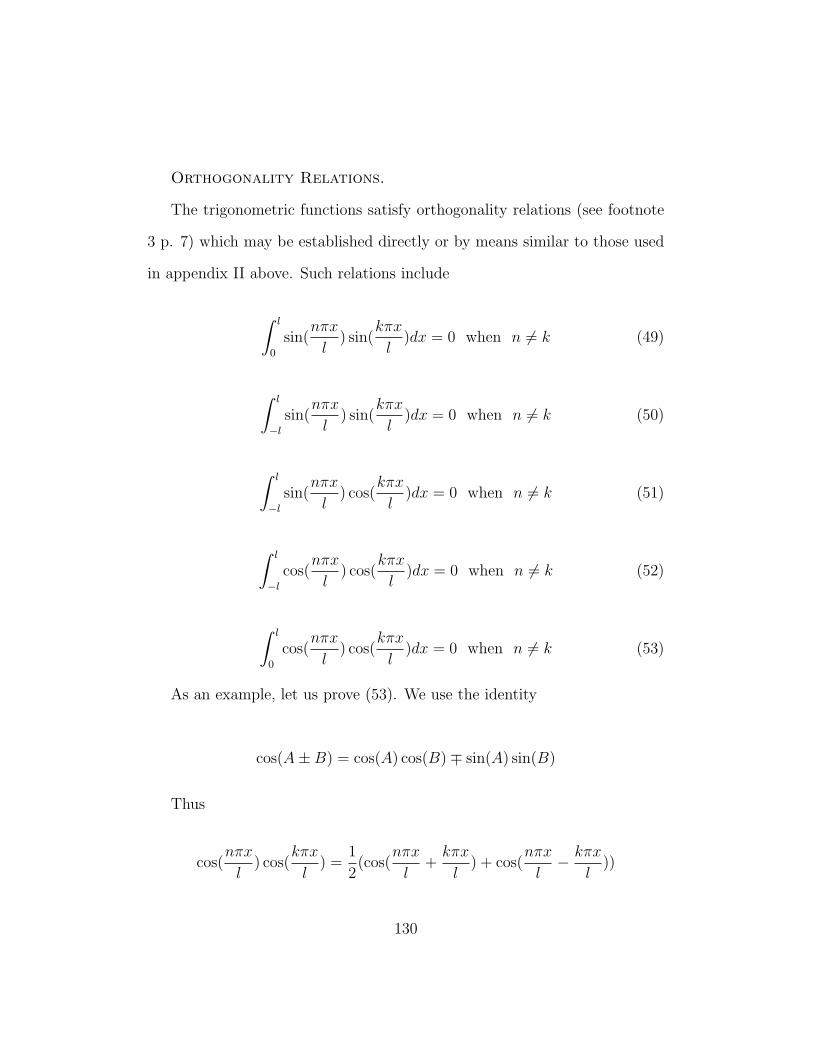
Orthogonality Relations.
The trigonometric functions satisfy orthogonality relations (see footnote
3 p. 7) which may be established directly or by means similar to those used
in appendix II above. Such relations include
∫ l
0
sin(nπx
l) sin(
kπx
l)dx = 0 when n 6= k (49)
∫ l
−lsin(
nπx
l) sin(
kπx
l)dx = 0 when n 6= k (50)
∫ l
−lsin(
nπx
l) cos(
kπx
l)dx = 0 when n 6= k (51)
∫ l
−lcos(
nπx
l) cos(
kπx
l)dx = 0 when n 6= k (52)
∫ l
0
cos(nπx
l) cos(
kπx
l)dx = 0 when n 6= k (53)
As an example, let us prove (53). We use the identity
cos(A±B) = cos(A) cos(B)∓ sin(A) sin(B)
Thus
cos(nπx
l) cos(
kπx
l) =
1
2(cos(
nπx
l+kπx
l) + cos(
nπx
l− kπx
l))
130
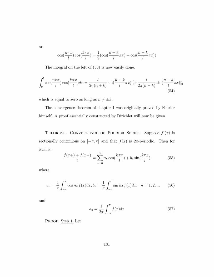
or
cos(nπx
l) cos(
kπx
l) =
1
2(cos(
n+ k
lπx) + cos(
n− kl
πx))
The integral on the left of (53) is now easily done:
∫ l
0
cos(nπx
l) cos(
kπx
l)dx =
l
2π(n+ k)sin(
n+ k
lπx)|l0+
l
2π(n− k)sin(
n− kl
πx)|l0
(54)
which is equal to zero as long as n 6= ±k.
The convergence theorem of chapter 1 was originally proved by Fourier
himself. A proof essentially constructed by Dirichlet will now be given.
Theorem - Convergence of Fourier Series. Suppose f ′(x) is
sectionally continuous on [−π, π] and that f(x) is 2π-periodic. Then for
each x,
f(x+) + f(x−)
2=∞∑k=0
ak cos(kπx
l) + bk sin(
kπx
l) (55)
where
an =1
π
∫ π
−πcosnxf(x)dx, bn =
1
π
∫ π
−πsinnxf(x)dx, n = 1, 2, ... (56)
and
a0 =1
2π
∫ π
−πf(x)dx (57)
Proof. Step 1. Let
131
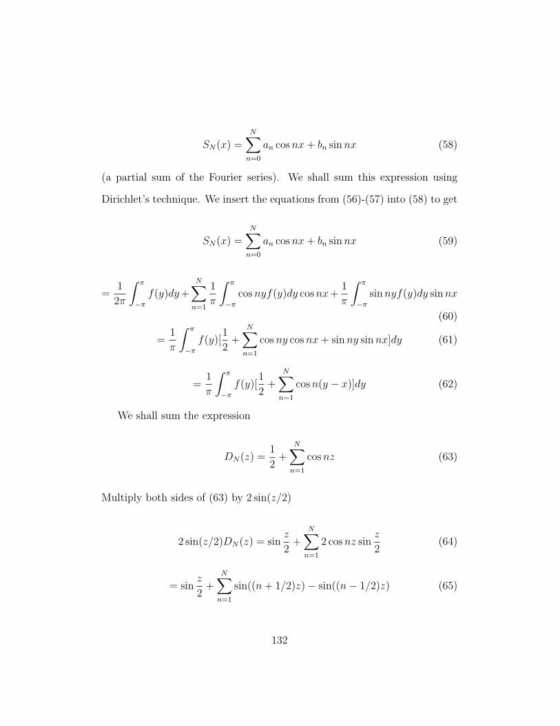
SN(x) =N∑n=0
an cosnx+ bn sinnx (58)
(a partial sum of the Fourier series). We shall sum this expression using
Dirichlet’s technique. We insert the equations from (56)-(57) into (58) to get
SN(x) =N∑n=0
an cosnx+ bn sinnx (59)
=1
2π
∫ π
−πf(y)dy+
N∑n=1
1
π
∫ π
−πcosnyf(y)dy cosnx+
1
π
∫ π
−πsinnyf(y)dy sinnx
(60)
=1
π
∫ π
−πf(y)[
1
2+
N∑n=1
cosny cosnx+ sinny sinnx]dy (61)
=1
π
∫ π
−πf(y)[
1
2+
N∑n=1
cosn(y − x)]dy (62)
We shall sum the expression
DN(z) =1
2+
N∑n=1
cosnz (63)
Multiply both sides of (63) by 2 sin(z/2)
2 sin(z/2)DN(z) = sinz
2+
N∑n=1
2 cosnz sinz
2(64)
= sinz
2+
N∑n=1
sin((n+ 1/2)z)− sin((n− 1/2)z) (65)
132
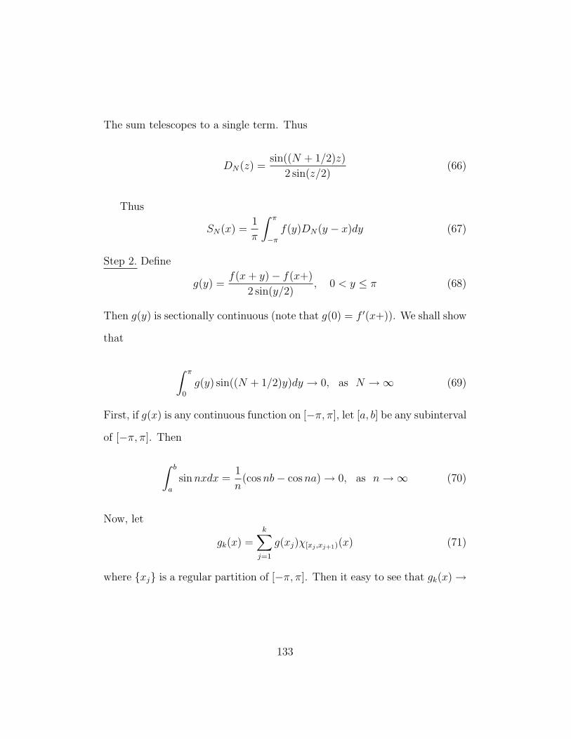
The sum telescopes to a single term. Thus
DN(z) =sin((N + 1/2)z)
2 sin(z/2)(66)
Thus
SN(x) =1
π
∫ π
−πf(y)DN(y − x)dy (67)
Step 2. Define
g(y) =f(x+ y)− f(x+)
2 sin(y/2), 0 < y ≤ π (68)
Then g(y) is sectionally continuous (note that g(0) = f ′(x+)). We shall show
that
∫ π
0
g(y) sin((N + 1/2)y)dy → 0, as N →∞ (69)
First, if g(x) is any continuous function on [−π, π], let [a, b] be any subinterval
of [−π, π]. Then
∫ b
a
sinnxdx =1
n(cosnb− cosna)→ 0, as n→∞ (70)
Now, let
gk(x) =k∑j=1
g(xj)χ[xj ,xj+1)(x) (71)
where xj is a regular partition of [−π, π]. Then it easy to see that gk(x)→
133
g(x) uniformly. Moreover (70) shows that
∫ π
−πgk(x) sin(nx)dx→ 0, as n→∞ (72)
Now observe ∫ π
−πg(x) sin(nx)dx (73)
=
∫ π
−πgk(x) sin(nx)dx−
∫ π
−πgk(x) sin(nx)dx−
∫ π
−πg(x) sin(nx)dx (74)
=
∫ π
−πgk(x) sin(nx)dx−
∫ π
−π(gk(x)− g(x)) sin(nx)dx (75)
Therefore
|∫ π
−πg(x) sin(nx)dx| ≤ |
∫ π
−πgk(x) sin(nx)dx|+
∫ π
−π|gk(x)− g(x)|| sin(nx)|dx
(76)
≤ |∫ π
−πgk(x) sin(nx)dx|+
∫ π
−π|gk(x)− g(x)|dx (77)
Given ε > 0, k sufficiently large
∫ π
−π|gk(x)− g(x)|dx < ε/2 (78)
Now let n be large enough so that
|∫ π
−πgk(x) sin(nx)dx| < ε/2 (79)
134
Then for all such n,
|∫ π
−πg(x) sin(nx)dx| < ε (80)
Since ε was arbitrary, this gives (69).41
Step 3. A direct computation based on (63) shows that
∫ π
−πDN(z)dz = 1 (81)
moreover, since (63) is an even function
1
2=
∫ π
0
DN(z)dz =
∫ 0
−πDN(z)dz (82)
Step 4.
SN(x) =1
π
∫ π
−πf(y)DN(y − x)dy =
1
π
∫ π
−πf(y)DN(y − x)dy (83)
=1
π
∫ π−x
−π−xf(t+ x)DN(t)dt =
1
π
∫ π
−πf(t+ x)DN(t)dt (84)
Step 5.
SN(x)− f(x+) + f(x−)
2=
1
π
∫ 0
−πf(x+ t)DN(t)dt− 1
2f(x−)
41Actually g being sectionally continuous, requires a slight modification of the proof,breaking up the integral over the intervals of continuity. The conclusion is the same.Moreover, the same conclusion holds for the cosine. The result of step 2 is a version ofthe “Riemann-Lebesgue Lemma” which holds for much less well-behaved functions g.
135
+1
π
∫ π
0
f(x+ t)DN(t)dt− 1
2f(x+)
Now
1
π
∫ 0
−πf(x+t)DN(t)dt−1
2f(x−) =
1
π
∫ 0
−πf(x+t)DN(t)dt− 1
π
∫ 0
−πDN(t)dtf(x−)
=1
π
∫ 0
−πf(x+ t)DN(t)dt− 1
π
∫ 0
−πf(x−)DN(t)dt
=1
π
∫ 0
−π(f(x+ t)− f(x−))DN(t)dt
By step 2, the last integral goes to zero as N → ∞. A similar statement
holds for
1
π
∫ π
0
f(x+ t)DN(t)dt− 1
2f(x+)
QED.
Corollary. If f(x) is an odd function, then only the sine terms appear
in the expansion. Alternatively, if f(x) is even, then only the cosine terms
appear in its Fourier series expansion.
Proof. This a simple consequence of (56), (57) above. In the odd case for
example, an will clearly be zero, since cosnxf(x) will be odd, therefore its
integral is even. Hence integrating over the symmetric interval must give zero.
Corollary. If f(x) is only defined on [0, π], it may be extended as
either an even or odd function to [−π, π]. Hence, it can be given a sine or
136
cosine expansion. Moreover in this case, the integrals in (56), (57) can be
written as integrals over [0, π].
The Fourier series itself is defined on all (−∞,∞) and therefore gives a
periodic extension of f(x) to all of R.
Corollary. The expansion theorem can be extended to functions satis-
fying the hypotheses of the theorem on any interval [−l, l]. The use of [−π, π]
was merely a convenience to reduce the size of expressions. Exactly the same
proof works for any symmetric interval. See page 7 for a version of this more
general case (for sine series).
A useful fact which we have (sometimes silently) employed throughout
the text is the following.
Theorem.42 Suppose un(x) is a sequence of continuous functions, each
defined on the interval [a, b]. Suppose further that the series
∞∑n=1
un(x)
converges uniformly to a function u(x). Then u(x) is continuous on [a, b].
42This theorem may seem obvious, but even the great Cauchy had trouble understandingit.
137

Moreover, if the functions un are differentiable and the series
∞∑n=1
dundx
converges uniformly on [a, b] then indeed dudx
exists and
∞∑n=1
dundx
=du
dx.
In order to understand the proof, we need a clear idea of uniform conver-
gence. We give the following adequate definition:
Definition of Uniform Convergence of a Sequence of Func-
tions. Let gn(x) be a sequence of functions defined on a set Ω. We say
the sequence gn(x) converges uniformly to a function g(x) on Ω if for any
ε > 0 ∃N such that if n ≥ N then |gn(x) − g(x)| < ε for all x ∈ Ω. Since
a series can be thought of in terms of the sequence of its partial sums, the
definition also applies to series, i.e. suppose we have a series∑un(x). To say
it converges uniformly to u(x) means that for any ε > 0 there is a positive
integer N such that if k ≥ N then
|k∑
n=1
un(x)− u(x)| < ε
for all x ∈ Ω.
Now we construct a proof of the theorem on uniform convergence. First
we dispose of the continuity of limits portion. So suppose each un(x) is
138
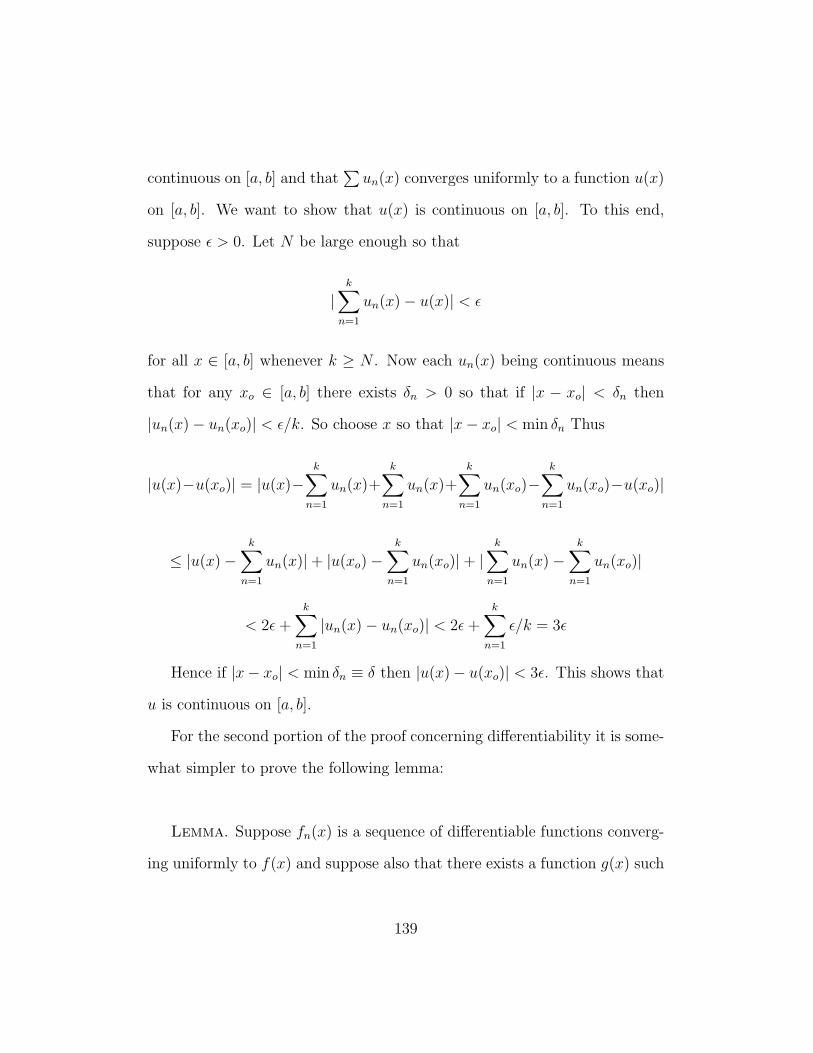
continuous on [a, b] and that∑un(x) converges uniformly to a function u(x)
on [a, b]. We want to show that u(x) is continuous on [a, b]. To this end,
suppose ε > 0. Let N be large enough so that
|k∑
n=1
un(x)− u(x)| < ε
for all x ∈ [a, b] whenever k ≥ N . Now each un(x) being continuous means
that for any xo ∈ [a, b] there exists δn > 0 so that if |x − xo| < δn then
|un(x)− un(xo)| < ε/k. So choose x so that |x− xo| < min δn Thus
|u(x)−u(xo)| = |u(x)−k∑
n=1
un(x)+k∑
n=1
un(x)+k∑
n=1
un(xo)−k∑
n=1
un(xo)−u(xo)|
≤ |u(x)−k∑
n=1
un(x)|+ |u(xo)−k∑
n=1
un(xo)|+ |k∑
n=1
un(x)−k∑
n=1
un(xo)|
< 2ε+k∑
n=1
|un(x)− un(xo)| < 2ε+k∑
n=1
ε/k = 3ε
Hence if |x− xo| < min δn ≡ δ then |u(x)− u(xo)| < 3ε. This shows that
u is continuous on [a, b].
For the second portion of the proof concerning differentiability it is some-
what simpler to prove the following lemma:
Lemma. Suppose fn(x) is a sequence of differentiable functions converg-
ing uniformly to f(x) and suppose also that there exists a function g(x) such
139
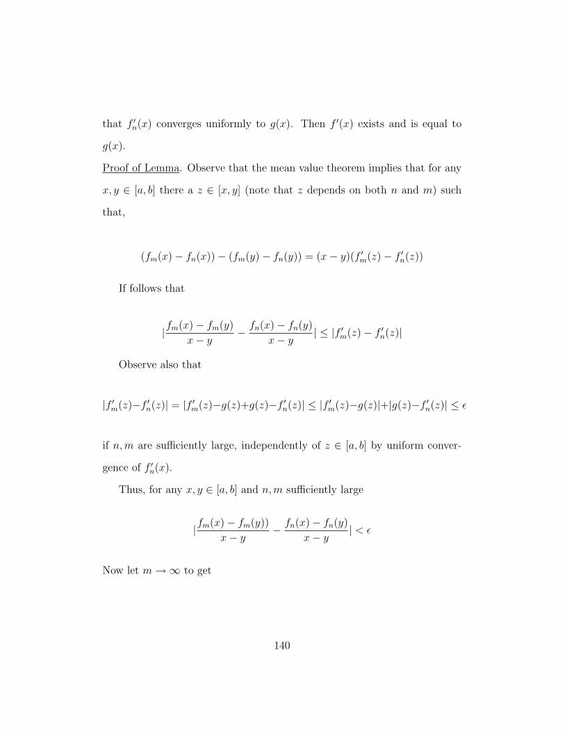
that f ′n(x) converges uniformly to g(x). Then f ′(x) exists and is equal to
g(x).
Proof of Lemma. Observe that the mean value theorem implies that for any
x, y ∈ [a, b] there a z ∈ [x, y] (note that z depends on both n and m) such
that,
(fm(x)− fn(x))− (fm(y)− fn(y)) = (x− y)(f ′m(z)− f ′n(z))
If follows that
|fm(x)− fm(y)
x− y− fn(x)− fn(y)
x− y| ≤ |f ′m(z)− f ′n(z)|
Observe also that
|f ′m(z)−f ′n(z)| = |f ′m(z)−g(z)+g(z)−f ′n(z)| ≤ |f ′m(z)−g(z)|+|g(z)−f ′n(z)| ≤ ε
if n,m are sufficiently large, independently of z ∈ [a, b] by uniform conver-
gence of f ′n(x).
Thus, for any x, y ∈ [a, b] and n,m sufficiently large
|fm(x)− fm(y))
x− y− fn(x)− fn(y)
x− y| < ε
Now let m→∞ to get
140
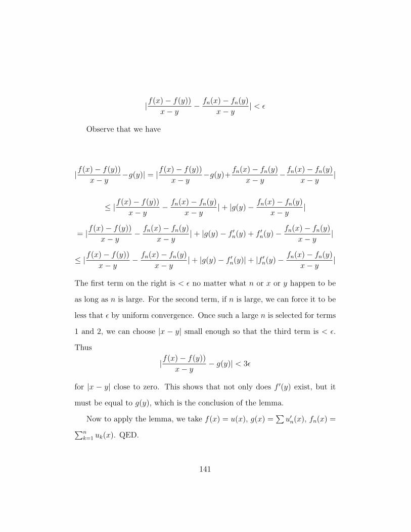
|f(x)− f(y))
x− y− fn(x)− fn(y)
x− y| < ε
Observe that we have
|f(x)− f(y))
x− y−g(y)| = |f(x)− f(y))
x− y−g(y)+
fn(x)− fn(y)
x− y− fn(x)− fn(y)
x− y|
≤ |f(x)− f(y))
x− y− fn(x)− fn(y)
x− y|+ |g(y)− fn(x)− fn(y)
x− y|
= |f(x)− f(y))
x− y− fn(x)− fn(y)
x− y|+ |g(y)− f ′n(y) + f ′n(y)− fn(x)− fn(y)
x− y|
≤ |f(x)− f(y))
x− y− fn(x)− fn(y)
x− y|+ |g(y)− f ′n(y)|+ |f ′n(y)− fn(x)− fn(y)
x− y|
The first term on the right is < ε no matter what n or x or y happen to be
as long as n is large. For the second term, if n is large, we can force it to be
less that ε by uniform convergence. Once such a large n is selected for terms
1 and 2, we can choose |x − y| small enough so that the third term is < ε.
Thus
|f(x)− f(y))
x− y− g(y)| < 3ε
for |x − y| close to zero. This shows that not only does f ′(y) exist, but it
must be equal to g(y), which is the conclusion of the lemma.
Now to apply the lemma, we take f(x) = u(x), g(x) =∑u′n(x), fn(x) =∑n
k=1 uk(x). QED.
141
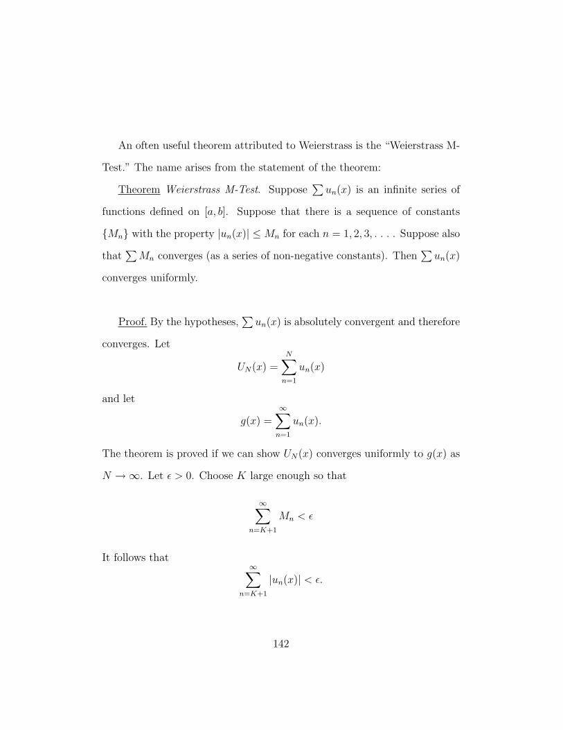
An often useful theorem attributed to Weierstrass is the “Weierstrass M-
Test.” The name arises from the statement of the theorem:
Theorem Weierstrass M-Test. Suppose∑un(x) is an infinite series of
functions defined on [a, b]. Suppose that there is a sequence of constants
Mn with the property |un(x)| ≤Mn for each n = 1, 2, 3, . . . . Suppose also
that∑Mn converges (as a series of non-negative constants). Then
∑un(x)
converges uniformly.
Proof. By the hypotheses,∑un(x) is absolutely convergent and therefore
converges. Let
UN(x) =N∑n=1
un(x)
and let
g(x) =∞∑n=1
un(x).
The theorem is proved if we can show UN(x) converges uniformly to g(x) as
N →∞. Let ε > 0. Choose K large enough so that
∞∑n=K+1
Mn < ε
It follows that∞∑
n=K+1
|un(x)| < ε.
142
Now we have
|g(x)−UK(x)| = |∞∑n=1
un(x)−K∑n=1
un(x)| = |∞∑
n=K+1
un(x)| ≤∞∑
n=K+1
|un(x)| < ε.
It follows that |g(x)− UN(x)| < ε for any N ≥ K. QED.
Remark 1. The test may be used with functions of more than one vari-
able. The proof is the same.
Remark 2. The theorem on uniform convergence is stated for functions
of one variable, but the following more general theorem has essentially the
same proof:
General Theorem on Uniform Convergence. Suppose that un(x) is a se-
quence of functions defined on an open subset Ω of Rk. Suppose also that∑un(x) converges uniformly on Ω, and that for some one of the variables of
x, say xi,∞∑n=1
∂u
∂xi(x)
converges uniformly. Then, if we define u(x) =∑un(x), it follows that
∂u
∂xi=∞∑n=1
∂un∂xi
for all x ∈ Ω.
143
Proof. The proof consists of reducing this general case to the one variable
proof. First, by hypothesis, Ω ⊆ Rk. Hence x ∈ Ω =⇒ x = (x1, x2, x3, ...xk).
Fix x ∈ Ω and consider a small box, Bδ = y ∈ Ω : yj = −δ ≤ xj ≤ δ ⊆ Ω
containing x. In the proof of the one variable case, replace [a, b] by [−δ, δ]
and x by xi.
144
Appendix IV - Limits
The purpose here is to give some brief definitions of useful limit ideas.
The most important are
lim sup and lim inf
To define these, we need to know what sup and inf are. Sup stands for
supremum, inf stands for infimum. These in turn are synonyms for least
upper bound and greatest lower bound respectively. It is a fact that any set
of real numbers has both a supremum and infimum. For example,
supx|x < 4 = 4
and
inf 1
n|n = 1, 2, 3, 4, . . . = 0
and
supx|x > 0 =∞
This brings us to the notions of lim sup and lim inf.
Let N(a, ε) = y|0 < |y − a| < ε then we define
lim supx→a
f(x) = limε→0
supf(x)|x ∈ N(a, ε)
145
Observe that when ε1 > ε2, f(x)|x ∈ N(a, ε1) ⊇ f(x)|x ∈ N(a, ε2).
Thus supf(x)|x ∈ N(a, ε1) ≥ supf(x)|x ∈ N(a, ε2). It follows that
lim supx→a
f(x)
always exists (∞ or −∞ are allowed possibilities) in contrast to ordinary
limits.
Similarly for lim inf,
lim infx→a
f(x) = limε→0
inff(x)|x ∈ N(a, ε)
whereas
inff(x)|x ∈ N(a, ε1) ≤ inff(x)|x ∈ N(a, ε2)
whenever ε1 > ε2.
When more than one variable is involved, the definitions remain essen-
tially the same.
Let N((a, b), ε) = (c, d)||(c, d)− (a, b)| < ε. Then we define
lim sup(x,t)→(a,b)
f(x, t) = limε→0
supf(x, t)||(x, t) ∈ N((a, b), ε)
In one variable, we can define one-sided limsup and liminf:
146
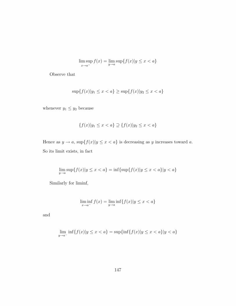
lim supx→a−
f(x) = limy→a
supf(x)|y ≤ x < a
Observe that
supf(x)|y1 ≤ x < a ≥ supf(x)|y2 ≤ x < a
whenever y1 ≤ y2 because
f(x)|y1 ≤ x < a ⊇ f(x)|y2 ≤ x < a
Hence as y → a, supf(x)|y ≤ x < a is decreasing as y increases toward a.
So its limit exists, in fact
limy→a
supf(x)|y ≤ x < a = infsupf(x)|y ≤ x < a|y < a
Similarly for liminf,
lim infx→a−
f(x) = limy→a
inff(x)|y ≤ x < a
and
limy→a−
inff(x)|y ≤ x < a = supinff(x)|y ≤ x < a|y < a
147
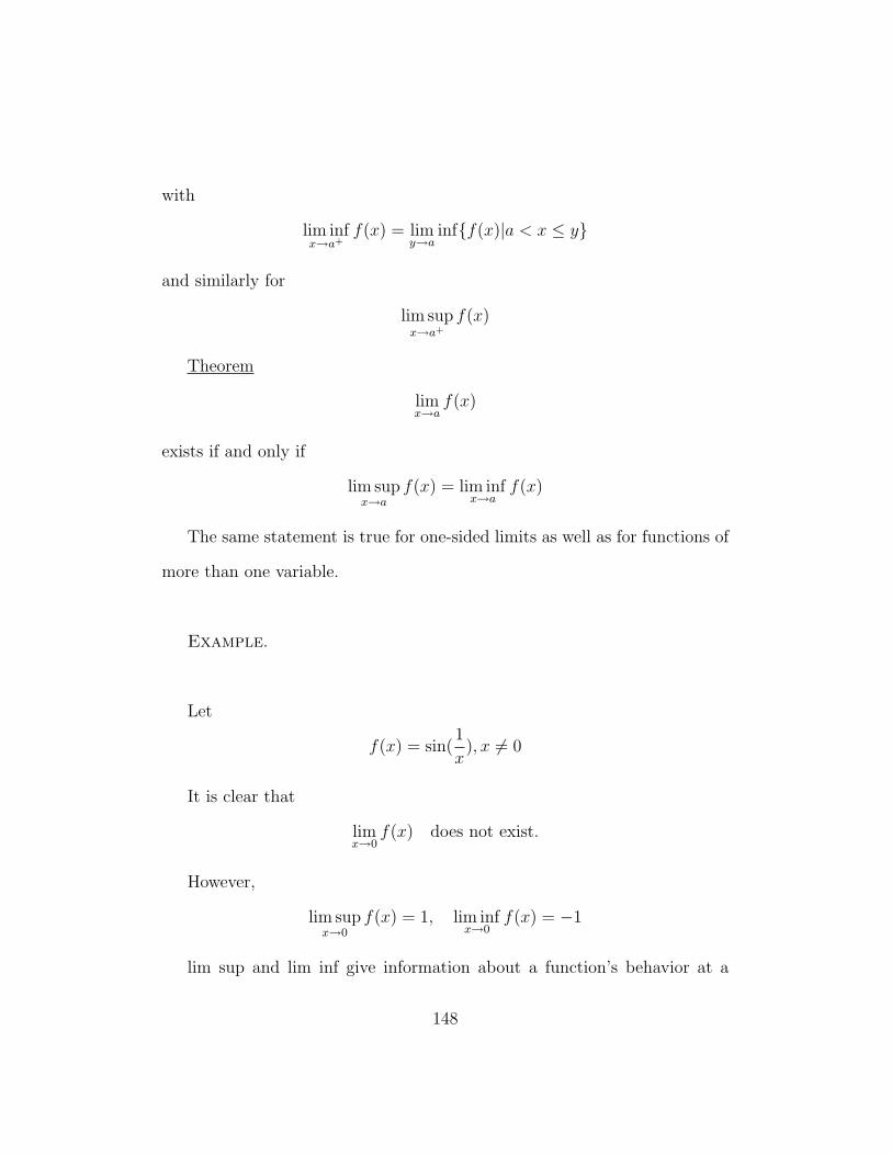
with
lim infx→a+
f(x) = limy→a
inff(x)|a < x ≤ y
and similarly for
lim supx→a+
f(x)
Theorem
limx→a
f(x)
exists if and only if
lim supx→a
f(x) = lim infx→a
f(x)
The same statement is true for one-sided limits as well as for functions of
more than one variable.
Example.
Let
f(x) = sin(1
x), x 6= 0
It is clear that
limx→0
f(x) does not exist.
However,
lim supx→0
f(x) = 1, lim infx→0
f(x) = −1
lim sup and lim inf give information about a function’s behavior at a
148
point and can be used to control or estimate such behavior as in Theorem 2
on page 91.
When more than one variable is involved, we don’t have a concept of
“one-sided” limit exactly, but sometimes it is useful to restrict the idea of
lim sup, lim inf in a somewhat similar way. For example,
lim supx→xo,t→0+
f(x, t)
would mean that we choose
N((xo, 0), ε) = (x, t) | 0 < |(x, t)− (xo, 0)| < ε, t > 0 and
lim supx→xo,t→0+
f(x, t) = limε→0
supf(x, t) | x ∈ N((xo, 0), ε)
———————————————————————
Promised extended argument from page 9 above:
To extend the argument a bit on uniform convergence of
∞∑n=1
−n2(π
l)2cn sin
nπx
le−k(nπ
l)2t
which is the (term by term) derivative of u(x, t), with respect to t, suggests
that we consider the following estimate:
| − cn(π
l)2n2 sin
nπx
le−k(nπ
l)2t| ≤ |cn|(
π
l)2n2 sin
nπx
le−k(nπ
l)2t
149
≤ n2e−k(nπl
)2t
provided n is large enough so that |cn|(πl )2 ≤ 1, say for all n ≥ m for some
m. Now fix to > 0 and δ > 0. For t > to + δ we claim that for large enough
n, that
n2e−k(nπl
)2t ≤ e−k(nπl
)2to
Let k(πl)2 = c. Restating, we have
n2e−cn2t ≤ e−cn
2to
This is equivalent to
n2e−cn2(t−to) ≤ 1
Now note that
n2e−cn2(t−to) ≤ n2e−cn
2δ
Observe that l’Hopital’s rule implies that
n2
ecn2δ→ 0
as n→∞. Thus for sufficiently large m, we have that if n ≥ m then
n2
ecn2δ≤ 1
150
or
n2e−cn2(t−to) ≤ 1
Taking Mn = e−cn2to gives us the correct hypothesis for the Weierstrass M-
test provided we can show that
∞∑n=m
Mn <∞
However l’Hopital’s rule again shows that
n2
ecn2to→ 0
as n→ 0 and therefore that
1
n2≥ e−cn
2to = Mn
for all large n and therefore
∞∑n=1
−n2(π
l)2cn sin
nπx
le−k(nπ
l)2t
converges uniformly. Actually we only established the estimate
|n2(π
l)2cn sin
nπx
le−k(nπ
l)2t| ≤Mn
for n ≥ m but this is sufficient. Now since to and δ were arbitrary, we
151
have term by term differentiability for all t. Also, since the second partial
derivative with respect to x of u(x, t) delivers a similar series, we have that
both sides of the heat equation are defined for u(x, t) (provided that f satisfies
the conditions of the Fourier convergence theorem).
152


![Elementary Di erential Geometry: Lecture Notes · [2] L. P. Eisenhart An introduction to di erential geometry with use of the ten-sor calculus, Princeton University Press. [3] W](https://img.pdfslide.us/doc/110x75/5f7de235dbee7e26cf5c8b7b/elementary-di-erential-geometry-lecture-notes-2-l-p-eisenhart-an-introduction.jpg)