Elementary Graph Theory

Robin Truax

March 2020

Contents

1 Basic Definitions 21.1 Specific Types of Graphs . . . . . . . . . . . . . . . . . . . . . . . . . . . . . . . . . . . 21.2 Paths and Cycles . . . . . . . . . . . . . . . . . . . . . . . . . . . . . . . . . . . . . . . 31.3 Trees and Forests . . . . . . . . . . . . . . . . . . . . . . . . . . . . . . . . . . . . . . . 31.4 Directed Graphs and Route Planning . . . . . . . . . . . . . . . . . . . . . . . . . . . . 4

2 Finding Cycles and Trails 52.1 Eulerian Circuits and Eulerian Trails . . . . . . . . . . . . . . . . . . . . . . . . . . . . 52.2 Hamiltonian Cycles . . . . . . . . . . . . . . . . . . . . . . . . . . . . . . . . . . . . . . 6

3 Planar Graphs 63.1 Polyhedra and Projections . . . . . . . . . . . . . . . . . . . . . . . . . . . . . . . . . . 73.2 Platonic Solids . . . . . . . . . . . . . . . . . . . . . . . . . . . . . . . . . . . . . . . . 8

4 Ramsey Theory 94.1 Ramsey’s Theorem . . . . . . . . . . . . . . . . . . . . . . . . . . . . . . . . . . . . . . 94.2 An Application of Ramsey’s Theorem . . . . . . . . . . . . . . . . . . . . . . . . . . . 104.3 Schur’s Theorem and a Corollary . . . . . . . . . . . . . . . . . . . . . . . . . . . . . . 10

5 The Lindstrom-Gessel-Viennot Lemma 115.1 Proving the Lindstrom-Gessel-Viennot Lemma . . . . . . . . . . . . . . . . . . . . . . 115.2 An Application in Linear Algebra . . . . . . . . . . . . . . . . . . . . . . . . . . . . . . 125.3 An Application in Tiling . . . . . . . . . . . . . . . . . . . . . . . . . . . . . . . . . . . 13

6 Coloring Graphs 136.1 The Five-Color Theorem . . . . . . . . . . . . . . . . . . . . . . . . . . . . . . . . . . . 14

7 Extra Topics 157.1 Matchings . . . . . . . . . . . . . . . . . . . . . . . . . . . . . . . . . . . . . . . . . . . 15

1

1 Basic Definitions

Definition 1 (Graphs). A graph G is a pair (V,E) where V is the set of vertices and E is a list of“edges” (undirected line segments) between pairs of (not necessarily distinct) vertices.

Definition 2 (Simple Graphs). A graph G is called a simple graph if there is at most one edgebetween any two vertices and if no edge starts and ends at the same vertex.

Below is an example of a very famous graph, called the Petersen graph, which happens to be simple:

Right now, our definitions have a key flaw: two graphs that have exactly the same setup, except onevertex is a quarter-inch to the left, are considered completely different. To solve this issue, we needan idea of “equivalence of graphs”.

Definition 3 (Graph Isomorphism). An isomorphism of graphs G = (VG, EG) and H = (VH , EH) isa bijection φ : VG → VH such that (v, w) is in EG if and only if (φ(v), φ(w)) is in EH . If there is anisomorphism φ : G→ H, we say G and H are isomorphic graphs, denoted G ∼= H.

Essentially, an isomorphism of graphs is a structure-preserving map from the set of vertices of G to theset of vertices of H which is a one-to-one correspondence. Of course, where there is an isomorphism,there is a homomorphism.

Definition 4 (Graph Homomorphism and Subgraphs). A homomorphism of graphs G = (VG, EG)and H = (VH , EH) is a function φ : VG → VH such that (v, w) ∈ EG ⇒ (φ(v), φ(w)) ∈ EH . Inparticular, if this is an injective function G→ H, then we say that H is a subgraph of G (since thereis a structure-preserving embedding of H into G).

1.1 Specific Types of Graphs

Definition 5 (Null Graph). The graph G with v vertices and no edges is called the null graph on vvertices and denoted Nv. For example, a diagram of the graph N0 is displayed to the right:

Definition 6 (Complete Graph). The graph G on v vertices with one edge between each distinct pairof vertices is called the complete graph on v vertices and denoted Kv.

Definition 7 (Bipartite Graph). A graph G is called a bipartite graph if one can partition the set ofvertices VG of G into two nonempty parts A and B such that every edge in G is between a vertex inA and a vertex in B.

For example, the “utility graph” (which we will explore more later) is a bipartite graph:

2

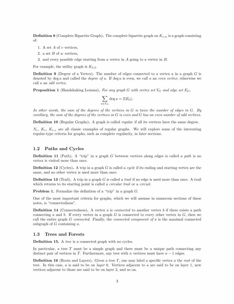
Definition 8 (Complete Bipartite Graph). The complete bipartite graph onKv,w is a graph consistingof:

1. A set A of v vertices,

2. a set B of w vertices,

3. and every possible edge starting from a vertex in A going to a vertex in B.

For example, the utility graph is K3,3.

Definition 9 (Degree of a Vertex). The number of edges connected to a vertex a in a graph G isdenoted by deg a and called the degree of a. If deg a is even, we call a an even vertex ; otherwise wecall a an odd vertex.

Proposition 1 (Handshaking Lemma). For any graph G with vertex set VG and edge set EG,∑a∈VG

deg a = 2|EG|.

In other words, the sum of the degrees of the vertices in G is twice the number of edges in G. Bycorollary, the sum of the degrees of the vertices in G is even and G has an even number of odd vertices.

Definition 10 (Regular Graphs). A graph is called regular if all its vertices have the same degree.

Nv, Kv, Kv,v are all classic examples of regular graphs. We will explore some of the interestingregular-type criteria for graphs, such as complete regularity, in later sections.

1.2 Paths and Cycles

Definition 11 (Path). A “trip” in a graph G between vertices along edges is called a path is novertex is visited more than once.

Definition 12 (Cycles). A trip in a graph G is called a cycle if its ending and starting vertex are thesame, and no other vertex is used more than once.

Definition 13 (Trail). A trip in a graph G is called a trail if no edge is used more than once. A trailwhich returns to its starting point is called a circular trail or a circuit.

Problem 1. Formalize the definition of a “trip” in a graph G.

One of the most important criteria for graphs, which we will assume in numerous sections of thesenotes, is “connectedness”.

Definition 14 (Connectedness). A vertex a is connected to another vertex b if there exists a pathconnecting a and b. If every vertex in a graph G is connected to every other vertex in G, then wecall the entire graph G connected. Finally, the connected component of a is the maximal connectedsubgraph of G containing a.

1.3 Trees and Forests

Definition 15. A tree is a connected graph with no cycles.

In particular, a tree T must be a simple graph and there must be a unique path connecting anydistinct pair of vertices in T . Furthermore, any tree with n vertices must have n− 1 edges.

Definition 16 (Roots and Layers). Given a tree T , one may label a specific vertex a the root of thetree. In this case, a is said to be on layer 0. Vertices adjacent to a are said to be on layer 1, newvertices adjacent to those are said to be on layer 2, and so on.

3

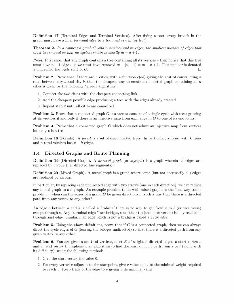
Definition 17 (Terminal Edges and Terminal Vertices). After fixing a root, every branch in thegraph must have a final terminal edge to a terminal vertex (or leaf ).

Theorem 2. In a connected graph G with n vertices and m edges, the smallest number of edges thatmust be removed so that no cycles remain is exactly m− n+ 1.

Proof. First show that any graph contains a tree containing all its vertices – then notice that this treemust have n− 1 edges, so we must have removed m− (n− 1) = m− n+ 1. This number is denotedγ and called the cycle rank of G.

Problem 2. Prove that if there are n cities, with a function c(ab) giving the cost of constructing aroad between city a and city b, then the cheapest way to create a connected graph containing all ncities is given by the following “greedy algorithm”:

1. Connect the two cities with the cheapest connecting link.

2. Add the cheapest possible edge producing a tree with the edges already created.

3. Repeat step 2 until all cities are connected.

Problem 3. Prove that a connected graph G is a tree or consists of a single cycle with trees growingat its vertices if and only if there is an injective map from each edge in G to one of its endpoints.

Problem 4. Prove that a connected graph G which does not admit an injective map from verticesinto edges is a tree.

Definition 18 (Forests). A forest is a set of disconnected trees. In particular, a forest with k treesand n total vertices has n− k edges.

1.4 Directed Graphs and Route Planning

Definition 19 (Directed Graph). A directed graph (or digraph) is a graph wherein all edges arereplaced by arrows (i.e. directed line segments).

Definition 20 (Mixed Graph). A mixed graph is a graph where some (but not necessarily all) edgesare replaced by arrows.

In particular, by replacing each undirected edge with two arrows (one in each direction), we can reduceany mixed graph to a digraph. An example problem to do with mixed graphs is the “one-way trafficproblem”: when can the edges of a graph G be given directions in such a way that there is a directedpath from any vertex to any other?

An edge e between a and b is called a bridge if there is no way to get from a to b (or vice versa)except through e. Any “terminal edges” are bridges, since their tip (the outer vertex) is only reachablethrough said edge. Similarly, an edge which is not a bridge is called a cycle edge.

Problem 5. Using the above definitions, prove that if G is a connected graph, then we can alwaysdirect the cycle edges of G (leaving the bridges undirected) so that there is a directed path from anygiven vertex to any other.

Problem 6. You are given a set V of vertices, a set E of weighted directed edges, a start vertex sand an end vertex t. Implement an algorithm to find the least difficult path from s to t (along withits difficulty), using the following method:

1. Give the start vertex the value 0.

2. For every vertex v adjacent to the startpoint, give v value equal to the minimal weight requiredto reach v. Keep track of the edge to v giving v its minimal value.

4

3. Iterate by assigning values to each vertex adjacent to a vertex covering in the last step. Whenevermultiple values can be assigned to a vertex, choose the minimal one. Again, keep track of theedges to each vertex giving them their minimal value.

4. Eventually, one gives the end vertex t a value, and can trace back the path using the previousedges recorded.

2 Finding Cycles and Trails

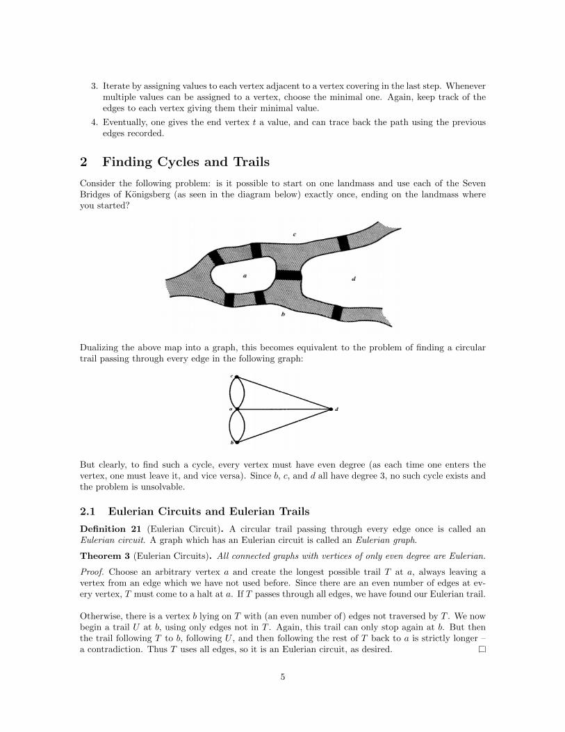
Consider the following problem: is it possible to start on one landmass and use each of the SevenBridges of Konigsberg (as seen in the diagram below) exactly once, ending on the landmass whereyou started?

Dualizing the above map into a graph, this becomes equivalent to the problem of finding a circulartrail passing through every edge in the following graph:

But clearly, to find such a cycle, every vertex must have even degree (as each time one enters thevertex, one must leave it, and vice versa). Since b, c, and d all have degree 3, no such cycle exists andthe problem is unsolvable.

2.1 Eulerian Circuits and Eulerian Trails

Definition 21 (Eulerian Circuit). A circular trail passing through every edge once is called anEulerian circuit. A graph which has an Eulerian circuit is called an Eulerian graph.

Theorem 3 (Eulerian Circuits). All connected graphs with vertices of only even degree are Eulerian.

Proof. Choose an arbitrary vertex a and create the longest possible trail T at a, always leaving avertex from an edge which we have not used before. Since there are an even number of edges at ev-ery vertex, T must come to a halt at a. If T passes through all edges, we have found our Eulerian trail.

Otherwise, there is a vertex b lying on T with (an even number of) edges not traversed by T . We nowbegin a trail U at b, using only edges not in T . Again, this trail can only stop again at b. But thenthe trail following T to b, following U , and then following the rest of T back to a is strictly longer –a contradiction. Thus T uses all edges, so it is an Eulerian circuit, as desired.

5

Corollary 3.1. A connected graph has a trail Tab covering all edges just once (which we call anEulerian trail) if and only if a and b are the only odd vertices.

Proof. Connect a and b with an edge, create a Eulerian cycle, and then drop the edge ab.

Theorem 4. A connected graph with 2k odd vertices contains a family of k distinct trails which,together, traverse all edges of the graph exactly once.

Proof. Let the odd vertices in the graph be denoted by a1, . . . , ak and b1, . . . , bk. When we add theedges a1b1, . . . akbk to the graph, all the vertices become even and we get an Eulerian cycle T . Whenthe edges are dropped out again, T breaks up into k separate trails, still covering all edges.

2.2 Hamiltonian Cycles

Definition 22 (Hamiltonian Cycles). A Hamiltonian cycle in a graph is a cycle that passes througheach of the vertices exactly once. A graph with a Hamiltonian cycle is called a Hamiltonian graph.

Though it is extremely easy to determine if a graph is Eulerian, finding a Hamiltonian cycle or evenshowing that one exists is extremely difficult (we have found no efficient general criterion). Indeed,the problem of finding a Hamiltonian cycle is known to be NP -complete (that is, if it is possible todo it in polynomial time, then P = NP ).

3 Planar Graphs

Definition 23 (Planar Graph). If a graph can be drawn on the plane in such a way that the edgeshave no intersections or common points except at the vertices, then we call it planar.

Problem 7. Prove that K5 is not planar using the Jordan Curve Theorem.

Problem 8. Prove that K3,3 is not planar using the Jordan Curve Theorem.

Theorem 5 (Euler’s Formula). For a connected planar graph G with V vertices, E edges, and Ffaces (including the infinite face), V − E + F = 2.

Proof. Induct on E: start with 0 edges (which implies one vertex) – for which the theorem clearlyholds – and add edges. Each time, you either add a new vertex with your edge or a new face withyour edge, keeping the sum V − E + F constant.

Theorem 6 (Fary’s Theorem). Any simple planar graph can be drawn without crossings in such away that all edges are straight line segments.

Theorem 7 (Kuratowski-Wagner Theorem). A subdivision of a graph is formed by subdividing itsedges into paths of one or more edges. Then a finite graph is planar if and only if it contains nosubgraph which is not a subdivision of K5 or K3,3.

I encourage you to learn more about the proofs of the above theorems, but we will not discuss theproofs here – they are quite long for the minimal reward (at least with respect to what we are goingto work on next).

Problem 9. Use the Kuratowski-Wagner Theorem to prove that the Petersen graph is not planar.

However, this is not an easy test to perform in general. Instead, usually one uses invariants of planargraphs to prove that a graph is not planar. For example, if G is a simple connected planar graph withv vertices and e edges, then e ≤ 3v − 6.

Problem 10. Prove that e ≤ 3v− 6 by adding edges to any planar graph until all faces are triangles,and then using Euler’s Formula.

Also look at this link which shows an amazing and beautiful way to draw planar graphs in planarform using algebraic graph theory.

6

3.1 Polyhedra and Projections

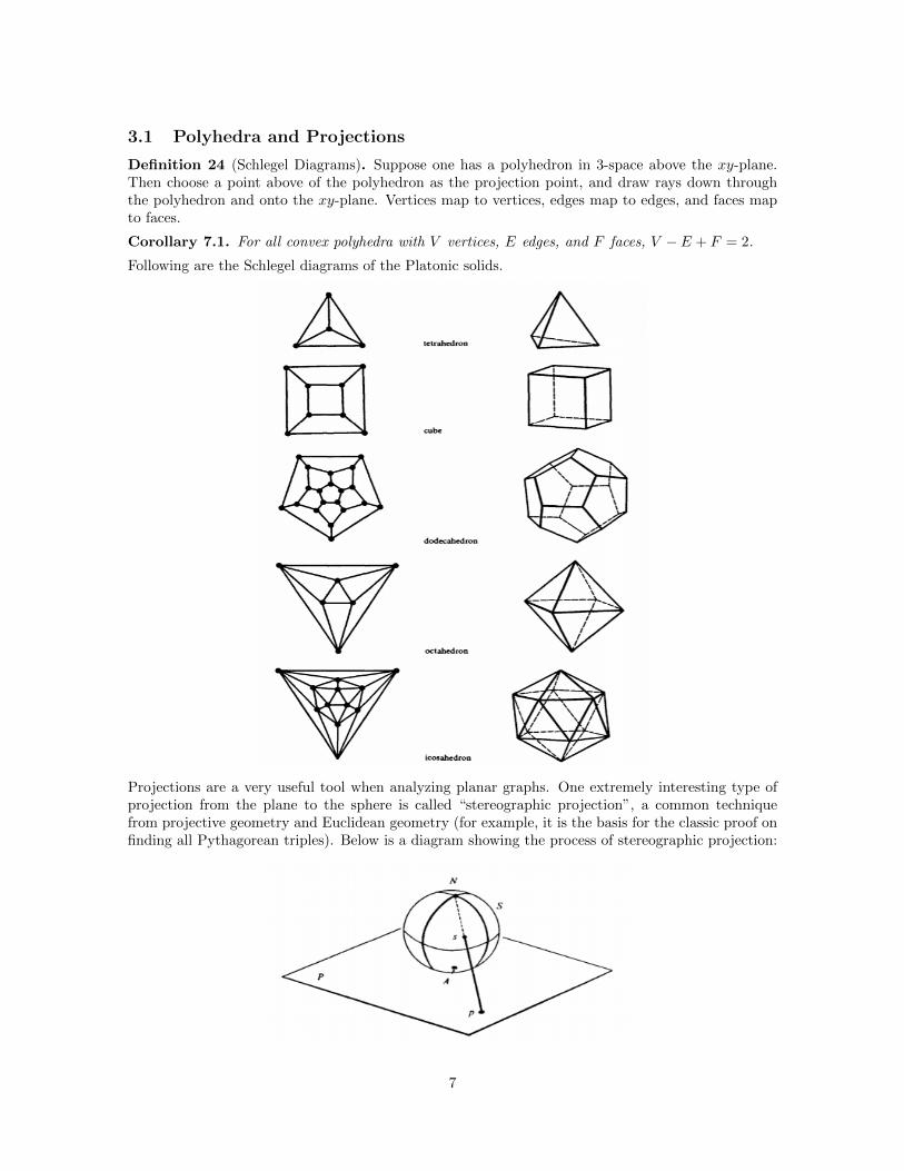
Definition 24 (Schlegel Diagrams). Suppose one has a polyhedron in 3-space above the xy-plane.Then choose a point above of the polyhedron as the projection point, and draw rays down throughthe polyhedron and onto the xy-plane. Vertices map to vertices, edges map to edges, and faces mapto faces.

Corollary 7.1. For all convex polyhedra with V vertices, E edges, and F faces, V − E + F = 2.

Following are the Schlegel diagrams of the Platonic solids.

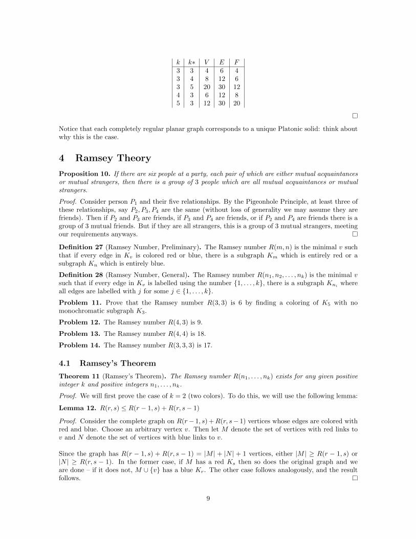
Projections are a very useful tool when analyzing planar graphs. One extremely interesting type ofprojection from the plane to the sphere is called “stereographic projection”, a common techniquefrom projective geometry and Euclidean geometry (for example, it is the basis for the classic proof onfinding all Pythagorean triples). Below is a diagram showing the process of stereographic projection:

7

Theorem 8. Let v be a vertex of a connected planar graph G. Then G can be embedded in the planein such a way that v is on the exterior face of the embedding.

Proof. Let G be a planar embedding of G. Stereographically project G onto the sphere to get anembedding into the sphere called X. Let f be a face that has v as one of its vertices: choose a pointx in the interior of f and fix it. Rotate the sphere until x is the north pole, and project X back downonto the plane. x becomes the point at infinity, so f is the exterior face, so v is on the exterior faceof the new planar embedding.

3.2 Platonic Solids

Definition 25 (Dual Graph). For any polygonal graph G, we can construct a new polygonal graphG∗ called its dual graph by the following method:

1. Within each face, including the infinite face, we define a single point.

2. Two such points are connected by an edge e if they correspond to neighboring faces (i.e. facessharing an edge f). e is drawn such that it crossings f but no other edges of the graph.

3. If there are several boundary edges common to the two faces, one new edge is drawn for eachboundary edge.

For example:

Notice that the two graphs have the same number of edges, but the number of vertices and faces isswapped. Also refer back to the figure of the Platonic solids’ Schleger diagrams and notice that theoctahedron graph is dual to the cube graph, the icosahedron graph is dual to the dodecahedron graph,and the tetrahedron graph is self-dual.

Definition 26 (Completely Regular). A graph G is completely regular if both G and G∗ are regular.

Theorem 9. There are exactly five completely regular graphs.

Proof. Suppose that G is regular of degree k and G∗ is regular of degree k∗. Then 2E = k · V and2E = k∗ · F . In partciular, E = kV

2 and F = kVk∗ . From Euler’s Formula, we see that:

n(1 +k

k∗− 1

2k) = 2⇒ n(2k + 2k∗ − kk∗) = 4k∗.

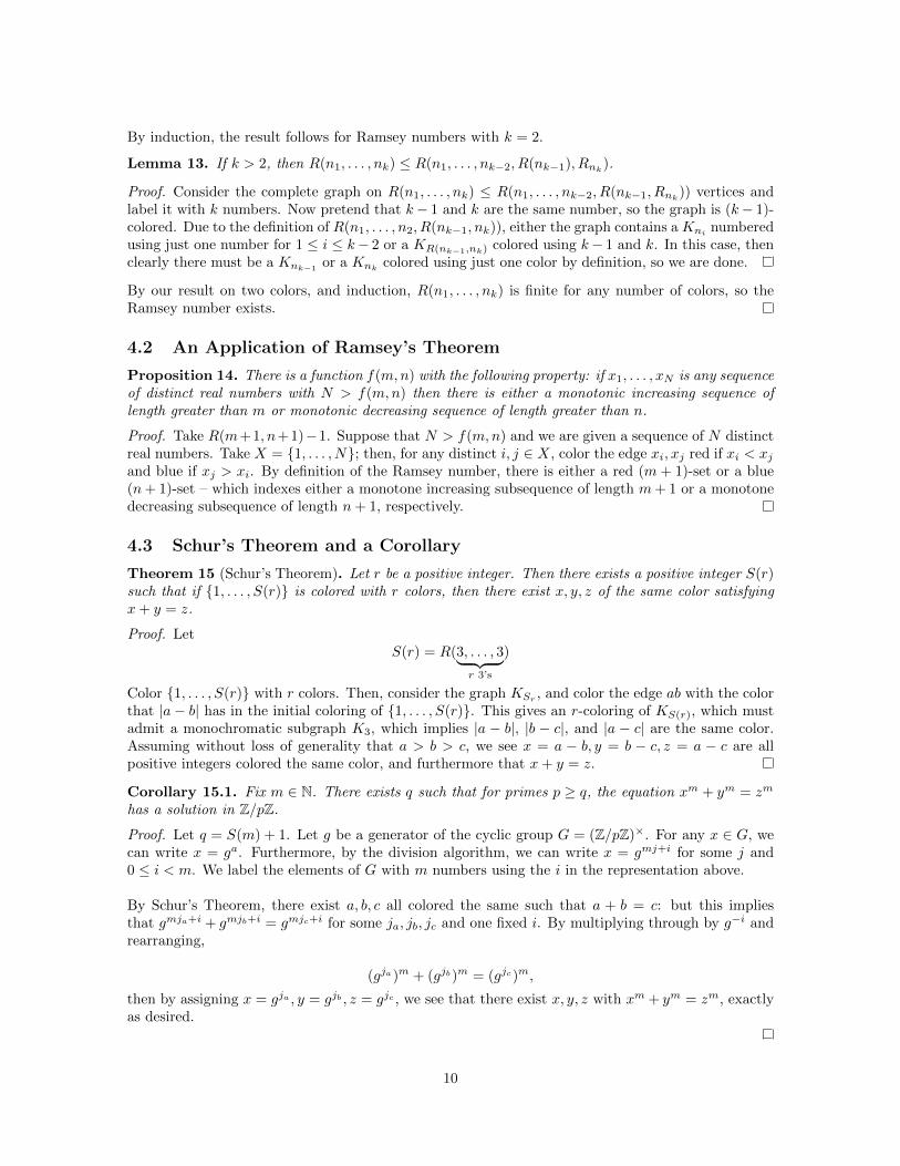
But since n and 4k∗ are positive integers, then the expression in parentheses must also be posi-tive. Thus 2k + 2k∗ − kk∗ > 0 and (k − 2)(k∗ − 2) < 4. The only pairs which work here are(3, 3), (3, 4), (3, 5), (4, 3), and (5, 3). From here, it is not difficult to show that there is only one graphfor each pair, as seen in the following table:

8

k k∗ V E F3 3 4 6 43 4 8 12 63 5 20 30 124 3 6 12 85 3 12 30 20

Notice that each completely regular planar graph corresponds to a unique Platonic solid: think aboutwhy this is the case.

4 Ramsey Theory

Proposition 10. If there are six people at a party, each pair of which are either mutual acquaintancesor mutual strangers, then there is a group of 3 people which are all mutual acquaintances or mutualstrangers.

Proof. Consider person P1 and their five relationships. By the Pigeonhole Principle, at least three ofthese relationships, say P2, P3, P4 are the same (without loss of generality we may assume they arefriends). Then if P2 and P3 are friends, if P3 and P4 are friends, or if P2 and P4 are friends there is agroup of 3 mutual friends. But if they are all strangers, this is a group of 3 mutual strangers, meetingour requirements anyways.

Definition 27 (Ramsey Number, Preliminary). The Ramsey number R(m,n) is the minimal v suchthat if every edge in Kv is colored red or blue, there is a subgraph Km which is entirely red or asubgraph Kn which is entirely blue.

Definition 28 (Ramsey Number, General). The Ramsey number R(n1, n2, . . . , nk) is the minimal vsuch that if every edge in Kv is labelled using the number {1, . . . , k}, there is a subgraph Kni

whereall edges are labelled with j for some j ∈ {1, . . . , k}.Problem 11. Prove that the Ramsey number R(3, 3) is 6 by finding a coloring of K5 with nomonochromatic subgraph K3.

Problem 12. The Ramsey number R(4, 3) is 9.

Problem 13. The Ramsey number R(4, 4) is 18.

Problem 14. The Ramsey number R(3, 3, 3) is 17.

4.1 Ramsey’s Theorem

Theorem 11 (Ramsey’s Theorem). The Ramsey number R(n1, . . . , nk) exists for any given positiveinteger k and positive integers n1, . . . , nk.

Proof. We will first prove the case of k = 2 (two colors). To do this, we will use the following lemma:

Lemma 12. R(r, s) ≤ R(r − 1, s) +R(r, s− 1)

Proof. Consider the complete graph on R(r− 1, s) +R(r, s− 1) vertices whose edges are colored withred and blue. Choose an arbitrary vertex v. Then let M denote the set of vertices with red links tov and N denote the set of vertices with blue links to v.

Since the graph has R(r − 1, s) + R(r, s − 1) = |M | + |N | + 1 vertices, either |M | ≥ R(r − 1, s) or|N | ≥ R(r, s − 1). In the former case, if M has a red Ks then so does the original graph and weare done – if it does not, M ∪ {v} has a blue Kr. The other case follows analogously, and the resultfollows.

9

By induction, the result follows for Ramsey numbers with k = 2.

Lemma 13. If k > 2, then R(n1, . . . , nk) ≤ R(n1, . . . , nk−2, R(nk−1), Rnk).

Proof. Consider the complete graph on R(n1, . . . , nk) ≤ R(n1, . . . , nk−2, R(nk−1, Rnk)) vertices and

label it with k numbers. Now pretend that k− 1 and k are the same number, so the graph is (k− 1)-colored. Due to the definition of R(n1, . . . , n2, R(nk−1, nk)), either the graph contains a Kni numberedusing just one number for 1 ≤ i ≤ k− 2 or a KR(nk−1,nk) colored using k− 1 and k. In this case, thenclearly there must be a Knk−1

or a Knkcolored using just one color by definition, so we are done.

By our result on two colors, and induction, R(n1, . . . , nk) is finite for any number of colors, so theRamsey number exists.

4.2 An Application of Ramsey’s Theorem

Proposition 14. There is a function f(m,n) with the following property: if x1, . . . , xN is any sequenceof distinct real numbers with N > f(m,n) then there is either a monotonic increasing sequence oflength greater than m or monotonic decreasing sequence of length greater than n.

Proof. Take R(m+1, n+1)−1. Suppose that N > f(m,n) and we are given a sequence of N distinctreal numbers. Take X = {1, . . . , N}; then, for any distinct i, j ∈ X, color the edge xi, xj red if xi < xjand blue if xj > xi. By definition of the Ramsey number, there is either a red (m + 1)-set or a blue(n+ 1)-set – which indexes either a monotone increasing subsequence of length m+ 1 or a monotonedecreasing subsequence of length n+ 1, respectively.

4.3 Schur’s Theorem and a Corollary

Theorem 15 (Schur’s Theorem). Let r be a positive integer. Then there exists a positive integer S(r)such that if {1, . . . , S(r)} is colored with r colors, then there exist x, y, z of the same color satisfyingx+ y = z.

Proof. LetS(r) = R(3, . . . , 3︸ ︷︷ ︸

r 3’s

)

Color {1, . . . , S(r)} with r colors. Then, consider the graph KSr, and color the edge ab with the color

that |a− b| has in the initial coloring of {1, . . . , S(r)}. This gives an r-coloring of KS(r), which mustadmit a monochromatic subgraph K3, which implies |a − b|, |b − c|, and |a − c| are the same color.Assuming without loss of generality that a > b > c, we see x = a − b, y = b − c, z = a − c are allpositive integers colored the same color, and furthermore that x+ y = z.

Corollary 15.1. Fix m ∈ N. There exists q such that for primes p ≥ q, the equation xm + ym = zm

has a solution in Z/pZ.

Proof. Let q = S(m) + 1. Let g be a generator of the cyclic group G = (Z/pZ)×. For any x ∈ G, wecan write x = ga. Furthermore, by the division algorithm, we can write x = gmj+i for some j and0 ≤ i < m. We label the elements of G with m numbers using the i in the representation above.

By Schur’s Theorem, there exist a, b, c all colored the same such that a + b = c: but this impliesthat gmja+i + gmjb+i = gmjc+i for some ja, jb, jc and one fixed i. By multiplying through by g−i andrearranging,

(gja)m + (gjb)m = (gjc)m,

then by assigning x = gja , y = gjb , z = gjc , we see that there exist x, y, z with xm + ym = zm, exactlyas desired.

10

5 The Lindstrom-Gessel-Viennot Lemma

Definition 29 (Locally Finite Graph). A locally finite graph is a graph with a (possibly infinite) setof vertices such that the set of edges of any single vertex is finite.

Definition 30 (Acyclic Graph). An acyclic graph is a graph with no cycles.

Definition 31 (Acyclic Plane). Consider the graph G with vertices Z2 with directed edges (x, y)→(x, y+ 1) and (x, y)→ (x+ 1, y). In particular, G is a locally finite directed acyclic graph and we callit the acyclic plane.

Definition 32 (Path System). Given “sources” a1, . . . , an and “sinks” b1, . . . , bn (both sets of distin-guished vertices) in a locally finite directed graph G, a path system P is an n-tuple of paths, sendingeach source to a distinct sink. Such a path system has an associated permutation: the permutationof {1, . . . , n} corresponding to which source goes to which sink. We denote this permutation σ(P).

Definition 33 (Non-Intersecting Path System). A path system is said to be a non-intersecting pathsystem if no two distinct paths share a vertex.

Lemma 16 (The Lindstrom-Gessel-Viennot Lemma). Consider a locally finite acyclic directed graphG with sources a1, . . . , an and sinks b1, . . . , bn. Define a weight on each edge e in G, denoted ω(e),and define the weight of a path P in G to be the product of the weights of the edges in P , denotedω(P ). For any two vertices a and b, define e(a, b) to be the sum of the weights of the paths between aand b.

Also let the weight of a path system P, denoted by ω(P), be∏P∈P ω(P ). Finally, let M be the matrix

whose i, j-entry is e(ai, bj). Then, if N is the set of all non-intersecting path systems in G,

detM =∑P∈N

sign(σ(P))ω(P)

Corollary 16.1. If the only possible permutation of a non-intersecting path system P is the identitypermutation, then detM =

∑P∈N

∏P∈P ω(P ).

Corollary 16.2. If the weight function is 1 (that is, the graph is unweighted) and furthermore theonly possible permutation of a non-intersecting path system is the identity, then detM is the numberof non-intersecting path systems in G.

5.1 Proving the Lindstrom-Gessel-Viennot Lemma

For such a complex theorem to state, the proof is remarkably simple. Intuitively, we start with theLeibniz formula for determinants, and then just need to define an involution on the path systems withfixes the non-intersecting path systems but reverses the sign of the permutation of the intersectingpath systems (so they all cancel out except the non-intersecting path systems).

Proof. Now recall the Leibniz formula for determinants: if A is a matrix with i, j entry ai,j , then

det(A) =∑σ∈Sn

sign(σ)

n∏i=1

ai,τ(i)

In particular, for our matrix M , we see that:

det(M) =∑σ∈Sn

sign(σ)

n∏i=1

e(ai, bσ(i)) =∑σ∈Sn

sign(σ)∑{ω(P) : P a path system with σ(P) = σ}

11

Now, if S is the set of all path systems in G, then the above sum (and therefore detM) is equal to:∑P∈S

sign(σ(P))ω(P)

Now we seek to prove that the given sum over all P ∈ S \N is 0. To do this, consider an involutionon the intersecting path systems defined so:

1. Let i be the smallest index such that the path from ai intersects another path and let j be thelargest index such that the path from aj intersects the path from ai.

2. Let v be the vertex which is the first intersection between the paths from ai and aj .

3. Swap the two paths (the path from ai and the path from aj) after v, thereby negating the signof the path system.

Clearly this is an involution, and since it negates the sign, we must have that the given sum over allP ∈ S \N is 0, as desired, so we have our desired result:

detM =∑P∈N

sign(σ(P))ω(P)

5.2 An Application in Linear Algebra

Theorem 17. Consider the following matrix:

M =

(00

) (11

) (22

). . .

(nn

)(10

) (21

) (32

). . .

(n+1n

)(20

) (31

) (42

). . .

(n+2n

)...

......

. . ....(

n0

) (n+11

) (n+22

). . .

(2nn

)

In short, we’re inserting Pascal’s triangle into a matrix – for example, for n = 4, the matrix becomes:

M =

1 1 1 11 2 3 41 3 6 101 4 10 20

For any n, the determinant of this matrix is 1.

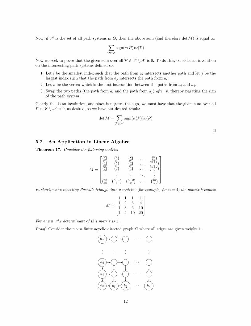
Proof. Consider the n× n finite acyclic directed graph G where all edges are given weight 1:

a0

a1

a2

an

b1 b2 bn. . .

......

...

. . .

. . .

. . .

...

12

Notice that there is no b0. However, we define b0 to be the same vertex as a0. It is not difficult tosee that the number of paths from ai to bj is the i, j-entry of M (indexing from 0 in the rows andcolumns). But notice that there is only one possible non-intersecting path system, where each aitravels right until it is directly above bi, and then travels downward. This path system is associatedwith the identity permutation, whence by the Lindstrom-Gessel-Viennot Lemma, detM = 1.

5.3 An Application in Tiling

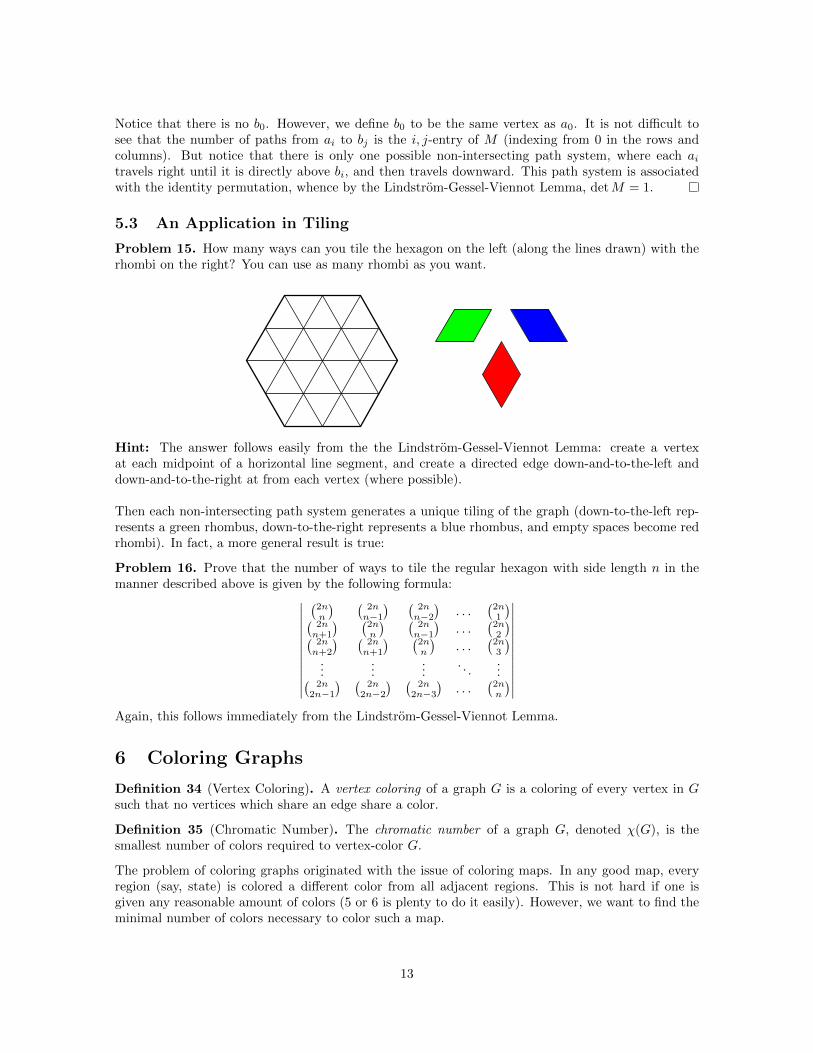
Problem 15. How many ways can you tile the hexagon on the left (along the lines drawn) with therhombi on the right? You can use as many rhombi as you want.

Hint: The answer follows easily from the the Lindstrom-Gessel-Viennot Lemma: create a vertexat each midpoint of a horizontal line segment, and create a directed edge down-and-to-the-left anddown-and-to-the-right at from each vertex (where possible).

Then each non-intersecting path system generates a unique tiling of the graph (down-to-the-left rep-resents a green rhombus, down-to-the-right represents a blue rhombus, and empty spaces become redrhombi). In fact, a more general result is true:

Problem 16. Prove that the number of ways to tile the regular hexagon with side length n in themanner described above is given by the following formula:∣∣∣∣∣∣∣∣∣∣∣∣

(2nn

) (2nn−1) (

2nn−2)

. . .(2n1

)(2nn+1

) (2nn

) (2nn−1)

. . .(2n2

)(2nn+2

) (2nn+1

) (2nn

). . .

(2n3

)...

......

. . ....(

2n2n−1

) (2n

2n−2) (

2n2n−3

). . .

(2nn

)

∣∣∣∣∣∣∣∣∣∣∣∣Again, this follows immediately from the Lindstrom-Gessel-Viennot Lemma.

6 Coloring Graphs

Definition 34 (Vertex Coloring). A vertex coloring of a graph G is a coloring of every vertex in Gsuch that no vertices which share an edge share a color.

Definition 35 (Chromatic Number). The chromatic number of a graph G, denoted χ(G), is thesmallest number of colors required to vertex-color G.

The problem of coloring graphs originated with the issue of coloring maps. In any good map, everyregion (say, state) is colored a different color from all adjacent regions. This is not hard if one isgiven any reasonable amount of colors (5 or 6 is plenty to do it easily). However, we want to find theminimal number of colors necessary to color such a map.

13

Our first step is to notice that because a map is naturally a planar graph, we can take the dual graphof the map to make our map coloring problem the following graph coloring problem.

Definition 36. A graph coloring is a coloring of every vertex in a graph such that no vertex whichshare an edge share a color.

Problem 17. How many colors are required to color a planar graph?

Of course, if we don’t restrict ourselves to planar graphs, there is no limit on the number of colorsrequired: the graph Kn requires n colors. Thus, this is the most interesting form of the graph coloringproblem.

Theorem 18 (The Four-Color Theorem). If G is a planar graph, then χ(G) ≤ 4.

This theorem, proven in 1976, is still not human-comprehensible: it requires the checking of over 600cases. Thus, we cannot document it here (and it is honestly not worth the effort to go through theproof). However, we will prove the Five-Color Theorem in the next subsection.

One common treatment of the chromatic number is via the chromatic polynomial, which is the functionfG on the natural numbers defined by fG(r) := {the number of colorings of G with r colors}. Thefact that we use the name chromatic “polynomial” should be surprising: it is not at all obvious thatsuch a function is a polynomial. We will prove now that this is the case:

Definition 37 (Deletions). Let e = ab be an edge of a graph G = (V,E). Then the graph G − e iscalled the deletion of e and equals (V,E \ {e}).

Definition 38 (Contractions). The contraction of e is denoted G/e and given by replacing x and yby a new vertex z and replacing any edge {v, x} or {v, y} with an edge {v, z} for every v.

Theorem 19. For any graph G with an edge e, fG(r) = fG−e(r)− fG/e(r)

Proof. Divide the set of colors of G− e into two disjoint classes:

1. Those for which x and y receive different colors: these are all valid colorings of G.

2. Those for which x and y receive the same color. These colorings correspond exactly to coloringsof G/e.

From this the result follows.

Corollary 19.1. This implies that the chromatic polynomial of G is a polynomial in Z[r] of degree n(where n is the number of vertices of G).

Proof. Consider the graph with one vertex and no edges, which has chromatic polynomial r and thussatisfies the condition. Then induction on the sum e + v (where v is the number of vertices and e isthe number of edges) gives the result for all graphs.

6.1 The Five-Color Theorem

Lemma 20. Every planar graph G contains a vertex v such that deg v ≤ 5.

Proof. Trivial from the bound e ≤ 3v − 6.

Theorem 21. For any planar graph G, χ(G) ≤ 5.

Proof. We induct on p, the number of vertices in G. If p = 1, then the chromatic number is 1. Nowsuppose that the theorem holds up through graphs of size P (that is, p ≤ P ⇒ χ(G) ≤ 5). Let G be agraph of order V + 1. By the lemma, there is a vertex v with deg v ≤ 5. By the inductive hypothesis,

14

G − v has a 5-coloring. If deg v ≤ 4, then there is a color which is not used by any of v’s neighbors,so we can color v and the result follows. Thus we may assume that deg v = 5.

Now notice that it is always possible to find 2 vertices adjacent to v that are not adjacent to eachother. If this was not the case, there would a subgraph of G isomorphic to K5, a contradiction withthe fact that G is planar.

Now let u and w be vertices adjacent to v but not each other. Form a graph H from G by identifyingu and w. Now, H is planar, because we can turn it into a plane graph by deforming u and w to valong uv and wv. Thus there is a 5-coloring for this graph, but that gives a 5-coloring on G− v whichhas 4 or fewer colors adjacent to v – so we can color the entirety of G by coloring v the last color.

7 Extra Topics

7.1 Matchings

Recall the definition of a bipartite graph from section 1. A key example of the application of sucha graph is the matching of applicants (set A) to positions (set P ). An edge is drawn between anapplicant and a position if the applicant is suitable for the job. Then, we seek to know when it ispossible for us to assign every applicant a to a position p ∈ P .

Definition 39 (Diversity Condition). For each group of k applicants (for all k = 1, 2, . . . , n), theremust be at least k jobs for which, collectively, they are qualified.

Theorem 22. If the diversity condition is fulfilled, one can assign a suitable job to each applicant.

Proof. Clearly the theorem is true for n = 1 and n = 2. We will thus try to prove the result byinduction: assume that the result is true for n− 1 applicants and fewer.

Case 1: Every possible group of k applicants (k = 1, 2, 3, . . . , n − 1) qualifies for more than k jobs.In this case, pick any one of the n applicants and place him in one of the jobs for which he is suited.Then the diversity condition holds for the remaining n− 1 applicants, so by induction there is a wayto put all of them too into suitable jobs.

Case 2: There is some possible set A0 of k0 applicants whose are qualified for exactly k0 jobs. Be-cause of the diversity condition, no k of these applications can be qualified for fewer than k jobs. Bythe induction hypothesis, the k0 applicants in A0 can be placed can be assigned suitable jobs.

But then the diversity conditions are still satisfied for the n − k0 applicants left (and the remainingjobs), so by induction the rest of the applicants can also be assigned jobs! Thus the result follows.

Definition 40 (Graph Matching). A graph matching from A into P on a bipartite graph is a setof edges such that each vertex in A is linked to a different vertex in P . Thus, the above theorembecomes: a matching of A into P is possible iff any k vertices in A are connected by edges to at leastk vertices in P .

There are numerous applications of this principle. Here’s a quite simple example:

Problem 18. Suppose that are n committees C1, . . . , Cn and a set of p1, . . . , pm people belongingto these committees. We seek to choose a secretary from each committee such that no person is asecretary for multiple committees. Prove that this is possible if and only if every group of k committeesincludes k distinct people.

Problem 19. Prove that if each committee has at least t members, and no individual belongs tomore than t committees, then it is always possible to find a separate secretary for each committee.

15