FACULTY OF ELECTRICAL ENGINEERING

UNIVERSITY OF BANJA LUKA

VOLUME 8, NUMBER 1, JUNE 20 41 1

ELECTRONICS

F A C U L T Y O F E L E C T R I C A L E N G I N E E R I N G

U N I V E R S I T Y O F B A N J A L U K A

Address: Patre 5, 78000 Banja Luka, Bosnia and Herzegovina

Phone: +387 51 211824

Fax: +387 51 211408

Web: www.etfbl.net

E L E C T R O N I C S Web: www.electronics.etfbl.net

E-mail: electronics@etfbl.net

Editor-in-Chief:

Branko L. Dokić, Ph. D.

Faculty of Electrical Engineering, University of Banja Luka, Bosnia and Herzegovina

E-mail: branko.dokic@etfbl.net

Co Editor-In-Chief:

Prof. Tatjana Pešić-Brđanin, University of Banja Luka, Bosnia and Herzegovina

E-mail: tatjanapb@etfbl.net

International Editorial Board: Prof. Goce Arsov, St. Cyril and Methodius University, Macedonia

Prof. Zdenka Babić, University of Banja Luka, Bosnia and Herzegovina

Prof. Petar Biljanović, University of Zagreb, Croatia

Prof. Milorad Božić, University of Banja Luka, Bosnia and Herzegovina

Prof. Octavio Nieto-Taladriz Garcia, Polytechnic University of Madrid, Spain

Dr Zoran Jakšić, IHTM, Serbia

Prof. Vladimir Katić, University of Novi Sad, Serbia

Prof. Tom J. Kazmierski, University of Southampton, United Kingdom

Prof. Vančo Litovski, University of Niš, Serbia

Dr Duško Lukač, University of Applied Sciences, Germany

Prof. Danilo Mandić, Imperial College, London, United Kingdom

Prof. Bratislav Milovanović, University of Niš, Serbia

Prof. Vojin Oklobdžija, University of Texas at Austin, USA

Prof. Predrag Pejović, University of Belgrade, Serbia

Prof. Ninoslav Stojadinović, University of Niš, Serbia

Prof. Robert Šobot, Western University, Canada

Prof. Slobodan Vukosavić, University of Belgrade, Serbia

Prof. Volker Zerbe, University of Applied Sciences of Erfurt, Germany

Secretary:

Mladen Knežić, M.Sc.

Željko Ivanović, M.Sc.

Publisher:

Faculty of Electrical Engineering, University of Banja Luka, Bosnia and Herzegovina

Number of printed copies: 100

HE oldest and the most prestigious expert association in

western Balkans, Serbia-based ETRAN Society has been

organizing conferences dedicated to various aspects of

electrical and electronics engineering since 1955. The

conference is split into 16 separate symposia, each dedicated

to a different aspect of electrical and electronics engineering.

For its 57th conference held in 2013 in Zlatibor, Serbia the

ETRAN Society introduced the best paper awards, where each

section grants its award to the best paper picked by a jury of

eminent members of the ETRAN Society, each of them expert

for the field covered by the section. Each section also chose

one outstanding presentation besides the awarded paper. For

this issue of Electronics journal we picked three such

presentations awarded at the ETRAN 2013 conference and

asked the authors to submit significantly extended and

rewritten versions of their manuscripts for this issue of

Electronics. The papers were further subject to the standard

reviewing procedure for Electronics. One of these

presentations was the award recipient in Electronics Section

(the paper by Miona Andrejević Stošović et al, dedicated to

simulation of maximum power point tracking in photovoltaic

systems), another in Automatics Section (the paper by Sanja

Vujnović et al dealing with the use of Bayesian networks in

thermal power plants), and one paper was chosen as the

outstanding presentation in Electronics Section (the paper by

Grigor Y. Zargaryan et al, dedicated to simulation and

verification of USB controllers). In this way the ETRAN

Society continues its already fruitful cooperation with the

ETRAN Society.

We are pleased to recommend readers of this issue of

Electronics journal to pay attention to the invited paper

„Energy Efficient Multi-Core Processing“ by C. Leech and T.

Kazmierski. In this paper, the present state of the art of energy-

efficient embedded processor design techniques is evaluated,

and it is demonstrated how small, variable architecture

embedded processors may exploit a run-time minimal

architectural synthesis technique to achieve greater energy and

area efficiency whilst maintaining performance.

The paper „Measuring Capacitor Parameters Using

Vector Network Analyzers“, by Deniss Stepins et al, is

focused on the measurement accuracy of capacitor parameters

using VNA (Vector Network Analyzers) and proper de-

embedding of an experimental setup parasitics to get accurate

measurement results.

Jasmin Igić and Milorad Božić in their paper present an

improvement of the Approximate Internal Model-based Neural

Control (AIMNC) structure. The authors also suggest an

approach in which one can ensure satisfactory behavior of the

AIMNC law for controlling slow industrial processes and

provide the zero steady state error in the cases of constant

reference signal and constant disturbances.

The two remaining papers, „Data-Driven Gradient Descent

Direct Adaptive Control for Discrete-Time Nonlinear SISO

Systems“ and „Integrated Cost-Benefit Assessment of

Customer-Driven Distributed Generation“, are related to the

research results published in the doctoral dissertations of Igor

Krčmar and Čedomir Željković, respectively.

Prof. Bratislav Milovanović

Chair of ETRAN Society

Prof. Zoran Jakšić

Chair of ETRAN Program Committee

Prof. Tatjana Pešić-Brđanin

Electronics journal Co Editor-In-Chief

Editorial

T

Energy Efficient Multi-Core ProcessingCharles Leech and Tom J. Kazmierski

(Invited Paper)

Abstract—This paper evaluates the present state of the artof energy-efficient embedded processor design techniques anddemonstrates, how small, variable-architecture embedded pro-cessors may exploit a run-time minimal architectural synthesistechnique to achieve greater energy and area efficiency whilstmaintaining performance. The picoMIPS architecture is pre-sented, inspired by the MIPS, as an example of a minimaland energy efficient processor. The picoMIPS is a variable-architecture RISC microprocessor with an application-specificminimised instruction set. Each implementation will contain onlythe necessary datapath elements in order to maximise areaefficiency. Due to the relationship between logic gate count andpower consumption, energy efficiency is also maximised in theprocessor therefore the system is designed to perform a specifictask in the most efficient processor-based form. The principlesof the picoMIPS processor are illustrated with an example ofthe discrete cosine transform (DCT) and inverse DCT (IDCT)algorithms implemented in a multi-core context to demonstratethe concept of minimal architecture synthesis and how it can beused to produce an application specific, energy efficient processor.

Index Terms—Embedded processors, application specific ar-chitectures, MIPS architecture, digital synthesis, energy efficientdesign, low power design.

Review PaperDOI: 10.7251/ELS1418003L

I. INTRODUCTION

THE energy efficiency of embedded processors is essentialin mobile electronics where devices are powered by

batteries. Processor performance has been increasing over thelast few decades at a rate faster than the developments inbattery technologies. This has led to a significant reductionof the battery life in mobile devices from days to hours. Also,new mobile applications demand higher performance and moregraphically intensive processing. These demands are currentlybeing addressed by many-core, high-frequency architectureswhich can deliver high-speed processing necessary to meet thetight execution deadlines. These two contradictory demands,the need to save energy and the requirement to deliver out-standing performance must be addressed by entirely new ap-proaches. A number of research directions have appeared. Het-erogeneous and reconfigurable embedded many-core systemscan improve energy efficiency while maintaining high speedthrough judicious task scheduling and hardware adaptability.In a heterogeneous system, such as the ARM big.LITTLEarchitecture [1] smaller cores are employed to process simpleand less demanding tasks to save energy while larger cores

Manuscript received 29 May 2014. Accepted for publication 12 June2014.

C. Leech and T. J. Kazmierski are with the University of Southampton, UK(e-mail: cl19g10, tjk@ecs.soton.ac.uk).

handle high performance and energy hungry processing whennecessary. Reconfigurable architectures use flexible intercon-nect, power gating and software control within each core, thusachieving heterogeneity within the core. Reconfigurable corescan be configured in this way as either slower, but energy effi-cient processors, or faster, high-performance cores.. A numberof approaches have been proposed to save energy within acore. Dynamic Voltage and Frequency Scaling (DVFS) [2] isa popular and well established technique where the supplyvoltage and the clock frequency are scaled to trade energy forperformance and vice-versa. DVFS is typically implementedby including voltage regulators and phase-lock loop controlledclocks in the processor. The architecture is modified to allowthe operating system to select a desired voltage and frequencythrough writing data to a DVFS control register. At any desiredperformance level, the operating system will put the processorinto a minimum energy consumption mode. DVFS has provedvery effective especially in applications where high perfor-mance is peaking only during a small fraction of the operatingtime as significant energy savings are achieved. Many otherenergy saving design techniques are currently being exploredat the circuit, architecture and even system level. For examplesupply voltage in bus drivers can be reduced to extremelylow levels to reduce bus energy consumption. New SRAMdesigns are being developed where energy consumption isreduced to extremely low levels in both the on-chip cachesand the external memories. The architecture of processor coresare traditionally determined from a compromise of speed,power consumption, scalability, maintainability and extensi-bility. However, applications have different characteristics thatrequire specific hardware implementations to enable optimalperformance and therefore a system should be able to adapt itsarchitecture to each application scenario. In this paper, we aimto demonstrate, through the evaluation of present technology,how small, variable-architecture embedded processors mayexploit a run-time minimal architectural synthesis technique toachieve greater energy and area efficiency whilst maintainingperformance.

II. OVERVIEW OF ENERGY EFFICIENCY TECHNOLOGIES

This section presents the current state of research in energyefficient technologies in multi-core systems for both traditionalpower saving techniques and novel technologies includingheterogeneous and reconfigurable architectures. Through theanalysis of present technology, we aim to demonstrate howa greater performance, energy efficiency and area efficiencybalance can be achieved.

The introduction of multi-core structures to processor ar-chitectures has caused a significant increase in the power

ELECTRONICS, VOL. 18, NO. 1, JUNE 2014 3

consumption of these systems. In addition, the gap betweenaverage power and peak power has widened as the levelof core integration increases [3]. A global power managerpolicy, such as that proposed by Isci et al, that has per-corecontrol of parameters such as voltage and frequency levels isrequired in order to provide effective dynamic control of thepower consumption [3]. Metrics such as performance-per-watt[4], [5], average and peak power or energy-delay product [6]are all used to quantify the power or energy efficiency of asystem in order to evaluate it, however properties are priori-tised differently depending on the application requirements.Modelling and simulation of multi-core processors is also animportant process in order to better understand the complexinteractions that occur inside a system and cause power andenergy consumption [7]–[11]. For example, the model createdby Basmadjian et al is tailored for multi-core architecturesin that it accounts for resource sharing and power savingmechanisms [8].

A. Energy Efficiency techniques in Static Homogeneous Multi-core Architectures

Many energy efficiency and power saving technologies arealready integrated into processor architectures in order toreduce power dissipation and extend battery life, especiallyin mobile devices. A combination of technologies is mostcommonly implemented to achieve the best energy efficiencywhilst still allowing the system to meet performance targets[4]. Techniques to increase energy efficiency can be appliedat many development levels from architecture co-design andcode compilation to task scheduling, run-time managementand application design [12]. A summary and analysis of thesetechnologies is presented in the following section.

1) Dynamic Voltage and Frequency Scaling: Dynamic Volt-age and Frequency Scaling (DVFS) is a technique used tocontrol the power consumption of a processor through fine ad-justment of the clock frequency and supply voltage levels [3],[4], [12], [13]. High levels are used when meeting performancetargets is a priority and low levels (known as CPU throttling)are used when energy efficiency is most important or high per-formance is not required. When the supply voltage is loweredand the frequency reduced, the execution of instructions bythe processor is slower but performed more energy efficientlydue to the extension of delays in the pipeline stages. Therise and fall times for logic circuitry is increased along withthe clock period meaning performance targets for applicationsmust be relaxed. DVFS can be used in homogeneous multi-core architectures to emulate heterogeneity by controlling thefrequency and supply to each core individually [14]. Each coretherefore appears as though it has different delay propertieshowever the architectures are still essentially identical. Thisper-core DVFS mechanism is investigated by Wonyoung et alwho conclude that significant energy saving opportunities existwhere on-chip integrated voltage regulators are used to providenanosecond scale voltage switching [13]. DVFS can also becombined with thread migration to reduce energy consumption[4], [15]. Cai et al cite the problem that present DVFSenergy saving techniques on multi-core systems assume one

hardware context for each core whereas simultaneous multi-threading (SMT) is commonly implemented which causesthese techniques to be less effective. Their novel technique,known as thread shuffling, uses concepts of thread criticalityand thread criticality degree instead of thread-delay to mapstogether threads with similar criticality degree. This accountsfor SMT when implementing DVFS and thread migrationand achieves energy savings of up to 56% without impedingperformance at all.

2) Clock Gating and Clock Distribution: Clock gating is aprocess, applied at the architectural design phase, to insertadditional logic between the clock source and clock inputof the processor’s circuitry. During program execution, itreduces power consumption by logically disconnecting theclock of synchronous logic circuits to prevent unnecessaryswitching. Classed as a Dynamic Power Management (DPM)technique, as it is applied at run-time along with othertechniques such as thread scheduling and DVFS to optimisethe power/performance trade-off of a system [12]. The clockgating and distribution techniques implemented by Qualcommin the Hexagon processor are analysed by Bassett et al ontheir ability to improve the energy efficiency of a digitalsignal processors (DSP) [16]. A low power clock networkis implemented using multi-level clock gating strategies andspine-based clock distribution. The 4 levels of clock gatingallows different size regions of the chip to be deactivated,from entire cores down to single logic cells. Further powerreduction is achieved through a structured clock tree that aimsto minimise the power consumed in distributing the clocksignal across the chip whilst avoiding clock skew and delay.The clock tree structure (CTS) examined by Bassett et al istested to give a 2 time reduction in skew over traditionalCTS while power tests show reductions in power consumptionby 8% for high-activity and over 35% for idle mode. Largeportions of the chip will spend the majority of their time inidle more therefore high efficiency in this mode is critical.

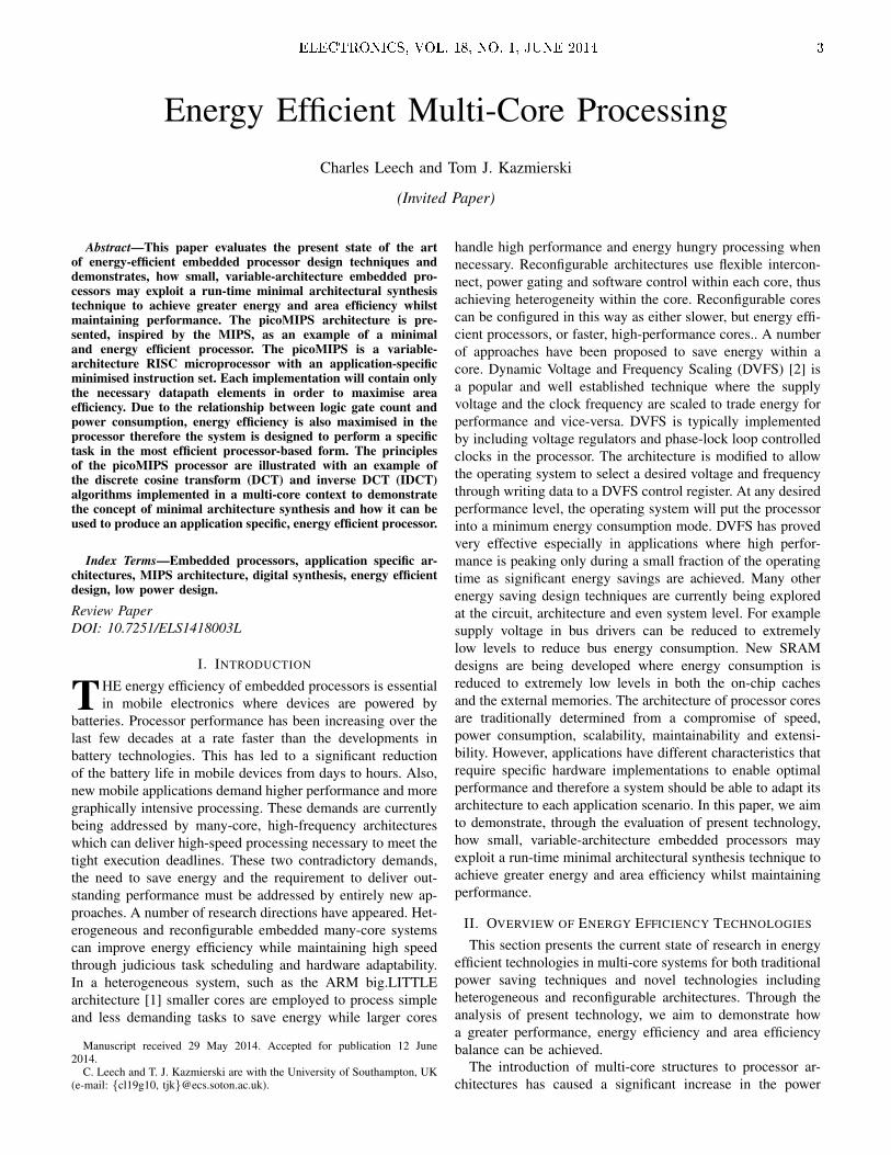
3) Power Domains: Power domains are regions of a systemor processor that are controlled from a single supply andcan be completely powered down in order to minimise powerconsumption without entirely removing the power supply tothe system. Power domains can be used dynamically andwhen used in conjunction with clock gating, lead to furtherimprovements in energy efficiency. The ARM Cortex-A15MPCore processor supports multiple power domains both forthe core and for the surrounding logic [17]. Figure 1 showsthese domains, labelled Processor and Non-Processor, thatallow large parts of the processor to be deactivated. Smallerinternal domains, such as CK GCLKCR, are implemented toallow smaller sections to be deactivated for finer performanceand power variations.

Power domains are often coupled with power modes as ameans of switching on or off several power domains in orderto enter low power, idle or shutdown states. The Cortex-A15features multiple power modes with specific power domainconfigurations such as Dormant mode, where some Debug andL2 cache logic is powered down but the L2 cache RAMs arepowered up to retain their state, or Powerdown mode whereall power domains are powered down and the processor state

4 ELECTRONICS, VOL. 18, NO. 1, JUNE 2014

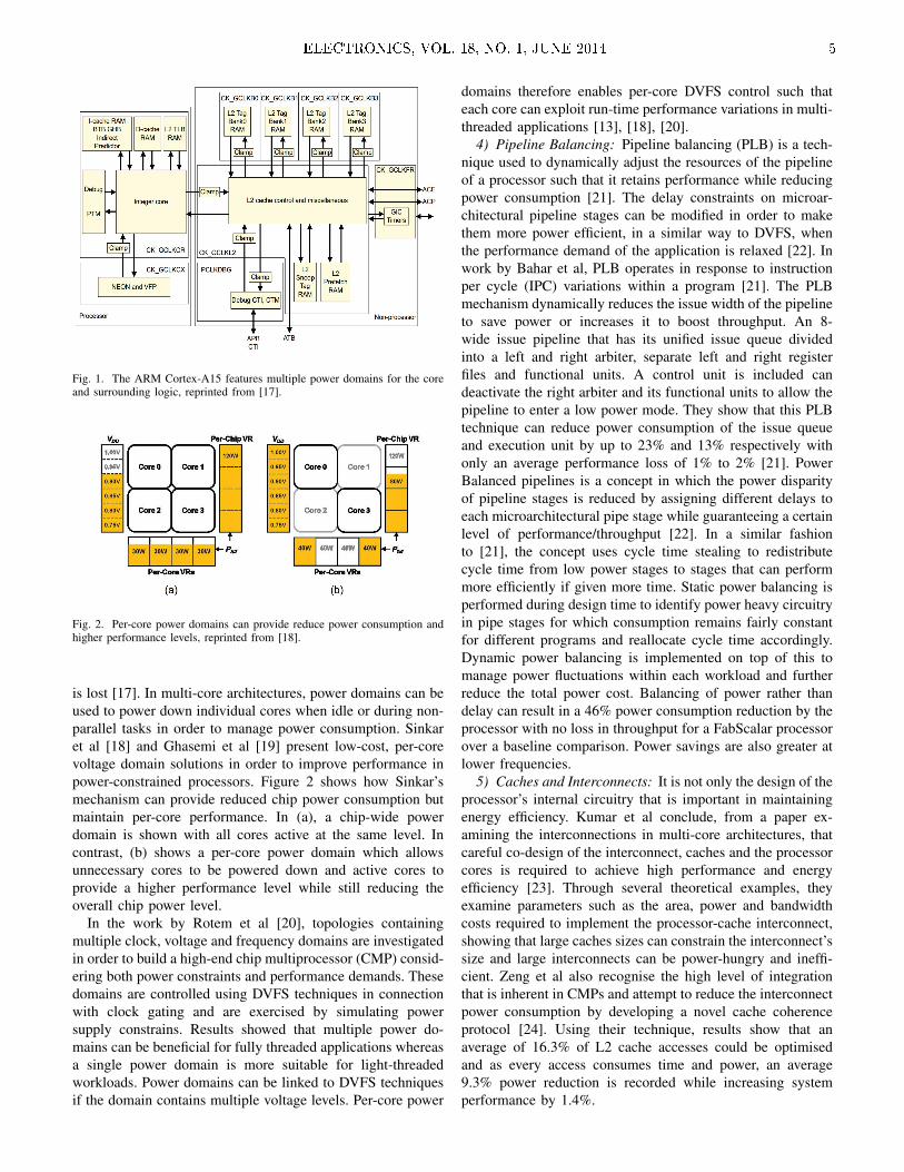
Fig. 1. The ARM Cortex-A15 features multiple power domains for the coreand surrounding logic, reprinted from [17].

Fig. 2. Per-core power domains can provide reduce power consumption andhigher performance levels, reprinted from [18].

is lost [17]. In multi-core architectures, power domains can beused to power down individual cores when idle or during non-parallel tasks in order to manage power consumption. Sinkaret al [18] and Ghasemi et al [19] present low-cost, per-corevoltage domain solutions in order to improve performance inpower-constrained processors. Figure 2 shows how Sinkar’smechanism can provide reduced chip power consumption butmaintain per-core performance. In (a), a chip-wide powerdomain is shown with all cores active at the same level. Incontrast, (b) shows a per-core power domain which allowsunnecessary cores to be powered down and active cores toprovide a higher performance level while still reducing theoverall chip power level.

In the work by Rotem et al [20], topologies containingmultiple clock, voltage and frequency domains are investigatedin order to build a high-end chip multiprocessor (CMP) consid-ering both power constraints and performance demands. Thesedomains are controlled using DVFS techniques in connectionwith clock gating and are exercised by simulating powersupply constrains. Results showed that multiple power do-mains can be beneficial for fully threaded applications whereasa single power domain is more suitable for light-threadedworkloads. Power domains can be linked to DVFS techniquesif the domain contains multiple voltage levels. Per-core power

domains therefore enables per-core DVFS control such thateach core can exploit run-time performance variations in multi-threaded applications [13], [18], [20].

4) Pipeline Balancing: Pipeline balancing (PLB) is a tech-nique used to dynamically adjust the resources of the pipelineof a processor such that it retains performance while reducingpower consumption [21]. The delay constraints on microar-chitectural pipeline stages can be modified in order to makethem more power efficient, in a similar way to DVFS, whenthe performance demand of the application is relaxed [22]. Inwork by Bahar et al, PLB operates in response to instructionper cycle (IPC) variations within a program [21]. The PLBmechanism dynamically reduces the issue width of the pipelineto save power or increases it to boost throughput. An 8-wide issue pipeline that has its unified issue queue dividedinto a left and right arbiter, separate left and right registerfiles and functional units. A control unit is included candeactivate the right arbiter and its functional units to allow thepipeline to enter a low power mode. They show that this PLBtechnique can reduce power consumption of the issue queueand execution unit by up to 23% and 13% respectively withonly an average performance loss of 1% to 2% [21]. PowerBalanced pipelines is a concept in which the power disparityof pipeline stages is reduced by assigning different delays toeach microarchitectural pipe stage while guaranteeing a certainlevel of performance/throughput [22]. In a similar fashionto [21], the concept uses cycle time stealing to redistributecycle time from low power stages to stages that can performmore efficiently if given more time. Static power balancing isperformed during design time to identify power heavy circuitryin pipe stages for which consumption remains fairly constantfor different programs and reallocate cycle time accordingly.Dynamic power balancing is implemented on top of this tomanage power fluctuations within each workload and furtherreduce the total power cost. Balancing of power rather thandelay can result in a 46% power consumption reduction by theprocessor with no loss in throughput for a FabScalar processorover a baseline comparison. Power savings are also greater atlower frequencies.

5) Caches and Interconnects: It is not only the design of theprocessor’s internal circuitry that is important in maintainingenergy efficiency. Kumar et al conclude, from a paper ex-amining the interconnections in multi-core architectures, thatcareful co-design of the interconnect, caches and the processorcores is required to achieve high performance and energyefficiency [23]. Through several theoretical examples, theyexamine parameters such as the area, power and bandwidthcosts required to implement the processor-cache interconnect,showing that large caches sizes can constrain the interconnect’ssize and large interconnects can be power-hungry and ineffi-cient. Zeng et al also recognise the high level of integrationthat is inherent in CMPs and attempt to reduce the interconnectpower consumption by developing a novel cache coherenceprotocol [24]. Using their technique, results show that anaverage of 16.3% of L2 cache accesses could be optimisedand as every access consumes time and power, an average9.3% power reduction is recorded while increasing systemperformance by 1.4%.

ELECTRONICS, VOL. 18, NO. 1, JUNE 2014 5

B. Energy Efficiency techniques in Heterogeneous Multi-coreArchitectures

A heterogeneous or asymmetric multi-core architecture iscomposed of cores of varying size and complexity which aredesigned to compliment each other in terms of performanceand energy efficiency [6]. A typical system will implement asmall core to process simple tasks, in an energy efficient way,while a larger core provides higher performance processingfor when computationally demanding tasks are presented.The cores represent different points in the power/performancedesign space and significant energy efficiency benefits can beachieved by dynamically allocating application execution tothe most appropriate core [25]. A task matching or switchingsystem is also implemented to intelligently assign tasks tocores; balancing a performance demand against maintainingsystem energy efficiency. These systems are particularly goodat saving power whilst handling a diverse workload where fluc-tuations of high and low computational demand are common[26].

A heterogeneous architecture can be created in many dif-ferent ways and many alternative have been developed dueto the heavy research interest in this area. Modifications togeneral purpose processors, such as asymmetric core sizes[11], custom accelerators [27], varied caches sizes [14] andheterogeneity within each core [5], [28], have all been demon-strated to introduce heterogeneous features into a system.

One of the most prominent and successful heterogeneousarchitectures to date is the ARM big.LITTLE system. Thisis a production example of a heterogeneous multiprocessorsystem consisting of a compact and energy efficient “LITTLE”Cortex-A7 processor coupled with a higher performance “big”Cortex-A15 processor [26]. The system is designed with thedynamic usage patterns of modern smart phones in mindwhere there are typically periods of high intensity processingfollowed by longer periods of low intensity processing [29].Low intensity tasks, such as texting and audio, can be handledby the A7 processor enabling a mobile device to save batterylife. When a period of high intensity occurs, the A15 processorcan be activated to increase the system’s throughput and meettighter performance deadlines. A power saving of up to 70%is advertised for a light workload, where the A7 processorcan handle all of the tasks, and a 50% saving for mediumworkloads where some tasks will require allocation to the A15processor.

Kumar et al present an alternative implementation wheretwo architectures from the Alpha family, the EV5 and EV6,are combined to be more energy and area efficient than ahomogeneous equivalent [6], [25]. They demonstrate that amuch higher throughput can be achieved due to the ability of aheterogeneous multi-core architecture to better exploit changesin thread-level parallelism as well as inter- and intra- threaddiversity [6]. In [25], they evaluate the system in terms of itspower efficiency indicating a 39% average energy reductionfor only a 3% performance drop [25].

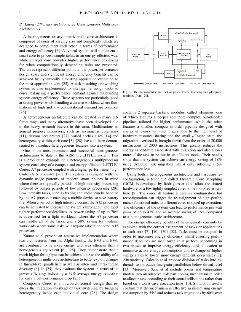
Composite Cores is a microarchitectural design that re-duces the migration overhead of task switching by bringingheterogeneity inside each individual core [28]. The design

Fig. 3. The microarchitecture for Composite Cores, featuring two µEngines,reprinted from [28].

contains 2 separate backend modules, called µEngines, oneof which features a deeper and more complex out-of-orderpipeline, tailored for higher performance, while the otherfeatures a smaller, compact in-order pipeline designed withenergy efficiency in mind. Figure Due to the high level ofhardware resource sharing and the small µEngine state, themigration overhead is brought down from the order of 20,000instructions to 2000 instructions. This greatly reduces theenergy expenditure associated with migration and also allowsmore of the task to be run in an efficient mode. Their resultsshow that the system can achieve an energy saving of 18%using dynamic task migration whilst only suffering a 5%performance loss.

Using both a heterogeneous architecture and hardware re-configuration, a technique called Dynamic Core Morphing(DCM) is developed by Rodrigues et al to allow the sharedhardware of a few tightly coupled cores to be morphed at run-time [5]. The cores all feature a baseline configuration butreconfiguration can trigger the re-assignment of high perfor-mance functional units to different cores to speed up execution.The efficiency of the system can lead to performance per wattgains of up to 43% and an average saving of 16% comparedto a homogeneous static architecture.

The energy efficiency benefits of heterogeneity can only beexploited with the correct assignment of tasks or applicationsto each core [7], [10], [30]–[32]. Tasks must be assigned inorder to maximise energy efficiency whilst ensuring perfor-mance deadlines are met. Awan et al perform scheduling intwo phases to improve energy efficiency; task allocation tominimise active energy consumption and exchange of higherenergy states to lower, more energy efficient sleep states [7].Alternatively, Calcado et al propose division of tasks into m-threads to introduce fine-grain parallelism below thread level[33]. Moreover, Saha et al include power and temperaturemodels into an adaptive task partitioning mechanism in orderto allocate task according to their actual utilisations rather thanbased on a worst case execution time [10]. Simulation resultsconfirm that the mechanism is effective in minimising energyconsumption by 55% and reduces task migrations by 60% over

6 ELECTRONICS, VOL. 18, NO. 1, JUNE 2014

alternative task partitioning schemes.Tasks assignment can also be performed in response to pro-

gram phases which naturally occur during execution when theresource demands of the application change. Phase detectionis used by Jooya and Analoui to dynamically re-assigningprograms for each phase to improve the performance andpower dissipation of heterogeneous multi-core processors [31].Programs are profiled in dynamic time intervals in order todetect phase changes. Sawalha et al also propose an onlinescheduling technique that dynamically adjusts the program-to-core assignment as application behaviour changes betweenphases with an aim to maximise energy efficiency [32].Simulated evaluation of the scheduler shows energy savingof 16% on average and up to 29% reductions in energy-delayproduct can be achieved as compared to static assignments.

C. Energy Efficiency techniques in Reconfigurable Multi-coreArchitectures

Reconfigurability is another property that has the potentialto increase the energy and area efficiency of processors andsystems on chip by introducing adaptability and hardware flex-ibility into the architecture. Building on the innovations thatheterogeneous architectures bring, reconfigurable architecturesaim to achieve both energy efficiency and high performancebut within the same processor and therefore meet the require-ments of many embedded systems. The flexible heterogeneousMulti-Core processor (FMC) is an example of the fusion ofthese two architectures that can deliver both a high throughputfor uniform parallel applications and high performance forfluctuating general purpose workloads [34]. Reconfigurablearchitectures are dynamic, adjusting their complexity, speedand performance level in response to the currently executingapplication. With this property in mind, we disregard systemsthat are statically reconfigurable but fixed while operating,such as traditional FPGAs, considering only architectures thatare run-time reconfigurable.

1) Dynamic Partial Reconfiguration: FPGA manufactur-ers such as Xilinx and Altera now offer a mechanismcalled Dynamic Partial Reconfiguration (DPR) [35] or Self-Reconfiguration (DPSR) [36] to enable reconfiguration duringrun-time of the circuits within an FPGA, allowing a regionof the design to change dynamically while other areas remainactive [37]. The FPGA’s architecture is partitioned into a staticregion consisting of fixed logic, control circuits and an embed-ded processor that control and monitor the system. The restof the design space is allocated to a dynamic/reconfigurableregion containing a reconfigurable logic fabric that can beformed into any circuit whenever hardware acceleration isrequired.

PDR/PDSR presents energy efficiency opportunities overfixed architectures. PDR enables the system to react dynam-ically to changes in the structure or performance and powerconstraints of the application, allowing it to address ineffi-ciencies in the allocation of resources and more accuratelyimplement changing software routines as dynamic hardwareaccelerators [35]. These circuits can then be easily removedor gated when they are no longer required to reduce power

consumption [38]. PDR can also increase the performanceof an FPGA based system because it permits the continuedoperation of portions of the dynamic region unaffected by re-configuration tasks. Therefore, it allows multiple applicationsto be run in parallel on a single FPGA [36]. This propertyalso improves the hardware efficiency of the system as, whereseparate devices were required, different tasks can now beimplemented on a single FPGA, reducing power consumptionand board dimensions. In addition, PDR reduces reconfigu-ration times due to the fact that only small modification aremade to the bitstream over time and the entire design does notneed to be reloaded for each change.

A study into the power consumption patterns of DPSR pro-gramming was conducted by Bonamy et al [9] to investigateto what degree the sharing of silicon area between multipleaccelerators will help to reduce power consumption. However,many parameters must be considered to assess whether theperformance improvement outweighs preventative factors suchas reconfiguration overhead, accelerator area and idle powerconsumption and as such any gain can be difficult to evaluate.Their results show complex variations in power usage atdifferent stages during reconfiguration that is dependent onfactors like the previous configuration and the contents ofthe configured circuit. In response to these experiments, threepower models are proposed to help analyse the trade-offbetween implementing tasks as dynamically reconfigurable, instatic configuration or in full software execution.

Despite clear benefits, several disadvantages become ap-parent with this form of reconfigurable technology. As wasshown above, the power consumption overhead associatedwith programming new circuits can effectively imposed aminimum size or usage time on circuits for implementationto be validated. In addition, a baseline power and area costis also always created due to the large static region whichcontinuously consumes power and can contain unnecessaryhardware. Finally, the FPGA interconnect reduces the speedand increases the power consumption of the circuit comparedto an ASIC implementation because of an increased gate countrequired to give the system flexibility.

2) Composable and Partitionable Architectures: Partition-ing and composition are techniques employed by some dynam-ically reconfigurable systems to provide adaptive parallel gran-ularity [39]. Composition involves synthesising a larger logicalprocessor from smaller processing elements when higher per-formance computation or greater instruction or thread levelparallelism (ILP or TLP) is required. Partitioning on the otherhand will divide up a large design in the most appropriateway and assign shared hardware resources to individual coresto meet the needs of an application.

Composable Lightweight Processors (CLP) is an exam-ple of a flexible architectural approach to designing a ChipMultiprocessor (CMP) where low-power processor cores canbe aggregated together dynamically to form larger single-threaded processors [39]. The system has an advantage overother reconfigurable techniques in that there are no mono-lithic structure spanning the cores which instead communicateusing a microarchitectural protocol. In tests against a fixed-granularity processor, the CLP has been shown to provide a

ELECTRONICS, VOL. 18, NO. 1, JUNE 2014 7

42% performance improvement whilst being on average 3.4times as area efficient and 2 times as power efficient.

Core Fusion is a similar technique to CLP in that it allowsmultiple processors to be dynamically allocated to a singleinstruction window and operated as if there were one largerprocessor [40]. The main difference from CLP is that CoreFusion operates on conventional RISC or CISC ISAs givingit an advantage over CLP in terms of compatibility. However,this also requires that the standard structures in these ISAs arepresent and so can limit the scalability of the architecture.

3) Coarse Grained Reconfigurable Array Architectures:Coarse-Grained Reconfigurable Array (CGRA) architecturesrepresent an important class of programmable system thatact as an intermediate state between fixed general purposeprocessors and fine-grain reconfigurable FPGAs. They aredesigned to be reconfigurable at a module or block level ratherthan at the gate level in order to trade-off flexibility for reducedreconfiguration time [41].

One example of a CGRA designed with energy efficiency asthe priority is the Ultra Low Power Samsung ReconfigurableProcessor (ULP-SRP) presented by Changmoo et al [42].Intended for biomedical applications as a mobile healthcaresolution, the ULP-SRP is a variation of the ADRES processor[43] and uses 3 run-time switch-able power modes and au-tomatic power gating to optimise the energy consumption ofthe device. Experimental results when running a low powermonitoring application show a 46.1% energy consumptionreduction compared to previous works.

III. CASE STUDY - PICOMIPS

In this section, we present the picoMIPS architecture asan example of a minimal and energy efficient processorimplementation. The key points of the architecture will bedescribed and evaluated, showing how it is a novel concept inminimal architecture synthesis. Developments are proposed tothe architecture, that can improve performance and maintainenergy efficiency, using the technologies described in theprevious section.

The picoMIPS architecture is foremost a RISC micropro-cessor with a minimised instruction set architecture (ISA).Each implementation will contain only the necessary datapathelements in order to maximise area efficiency as the priority.For example, the instruction decoder will only recogniseinstructions that the user specifies and the ALU will onlyperform the required logic or arithmetic functions. Due tothe proportionality between logic gate count and power con-sumption, energy efficiency is also maximised in the processortherefore the system is designed to perform a specific task inthe most efficient processor-based form.

By synthesising the picoMIPS as a microprocessor, a base-line configuration is established upon which functionality canbe added or removed, in the form of instructions or functions,while incurring only minimal changes to the area consumptionof the design. If the task was implemented as a specificdedicated hardware circuit, any changes to the functionalitycould have a large influence on the area consumption ofthe design. Figure 4 shows an example configuration for the

picoMIPS which can accommodate the majority of the simpleRISC instructions. It is a Harvard architecture, with separateprogram and data memories, although the designer may chooseto exclude a data memory entirely. The user can also specifythe widths of each data bus to avoid unnecessary opcode bitsfrom wasting logic gates.

The principles of the picoMIPS processor have been im-plemented in a few projects to demonstrate the concept ofminimal architecture synthesis and how it can be used toproduce an application specific, energy efficient processor. Thediscrete cosine transform (DCT) algorithm, a stage in JPEGcompression, was synthesised into a processor architecturebased on the picoMIPS concept. The resulting processor wasmore area efficient than a GPP due to the removal of un-necessary circuitry however its functionality was also reducedto performing only those functions which appear in the DCTalgorithm. The processor can also be compared to a dedicatedASIC hardware implementation of the DCT algorithm. AnASIC implementations have a much higher performance andthroughput of data however this is at the cost of area andenergy efficiency. The picoMIPS therefore represents a balancebetween the two, sacrificing some performance for area andenergy efficiency benefits.

The picoMIPS has also been implemented to perform theDCT and inverse DCT (IDCT) in a multi-core context [44]. Ahomogeneous architecture was deployed with the same singlecore structure, as in figure 4, being replicated 3 times. Thecores are connected via a data bus to a distribution module asshown in figure 5 where block data is transferred to each corein turn. This structure theoretically triples the throughput ofthe system as it can process multiple data blocks in parallel.

As a microprocessor architecture, the picoMIPS can im-plement many of the technologies discussed in section IIin order to improve energy efficiency. Clock gating, powerdomains and DVFS will all benefit the system however thearea overhead of implementing them must first be consideredas necessary. Pipeline balancing and caching can be integratedinto more complex picoMIPS architectures however these areperformance focused improvements and so are not prioritiesin the picoMIPS concept. The expansion of the system tomulti-core is also one that can be employed to improveperformance. Moreover, a heterogeneous architecture couldbe implemented to allow the picoMIPS to process multipledifferent applications simultaneously using several tailoredISAs. Reconfigurability can also be applied to picoMIPS tocreate an architecture which can be specific to each applicationthat is executed, effectively creating a general purpose yet ap-plication specific processor. This property would require run-time synthesis algorithms to detect and develop the instructionsand functional units that are required, before executing theapplication.

IV. CONCLUSION

A new concept of variable-architecture application-specificapproach to embedded processor design has been presented.Over the past few decades, the trend in processor architectures,has evolved from single core to homogeneous multi-core and

8 ELECTRONICS, VOL. 18, NO. 1, JUNE 2014

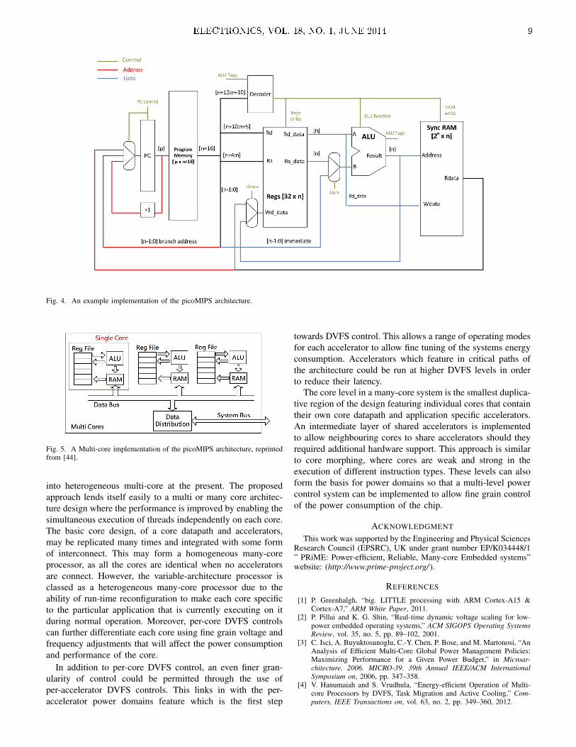
Fig. 4. An example implementation of the picoMIPS architecture.

Fig. 5. A Multi-core implementation of the picoMIPS architecture, reprintedfrom [44].

into heterogeneous multi-core at the present. The proposedapproach lends itself easily to a multi or many core architec-ture design where the performance is improved by enabling thesimultaneous execution of threads independently on each core.The basic core design, of a core datapath and accelerators,may be replicated many times and integrated with some formof interconnect. This may form a homogeneous many-coreprocessor, as all the cores are identical when no acceleratorsare connect. However, the variable-architecture processor isclassed as a heterogeneous many-core processor due to theability of run-time reconfiguration to make each core specificto the particular application that is currently executing on itduring normal operation. Moreover, per-core DVFS controlscan further differentiate each core using fine grain voltage andfrequency adjustments that will affect the power consumptionand performance of the core.

In addition to per-core DVFS control, an even finer gran-ularity of control could be permitted through the use ofper-accelerator DVFS controls. This links in with the per-accelerator power domains feature which is the first step

towards DVFS control. This allows a range of operating modesfor each accelerator to allow fine tuning of the systems energyconsumption. Accelerators which feature in critical paths ofthe architecture could be run at higher DVFS levels in orderto reduce their latency.

The core level in a many-core system is the smallest duplica-tive region of the design featuring individual cores that containtheir own core datapath and application specific accelerators.An intermediate layer of shared accelerators is implementedto allow neighbouring cores to share accelerators should theyrequired additional hardware support. This approach is similarto core morphing, where cores are weak and strong in theexecution of different instruction types. These levels can alsoform the basis for power domains so that a multi-level powercontrol system can be implemented to allow fine grain controlof the power consumption of the chip.

ACKNOWLEDGMENT

This work was supported by the Engineering and Physical SciencesResearch Council (EPSRC), UK under grant number EP/K034448/1” PRiME: Power-efficient, Reliable, Many-core Embedded systems”website: (http://www.prime-project.org/ ).

REFERENCES

[1] P. Greenhalgh, “big. LITTLE processing with ARM Cortex-A15 &Cortex-A7,” ARM White Paper, 2011.

[2] P. Pillai and K. G. Shin, “Real-time dynamic voltage scaling for low-power embedded operating systems,” ACM SIGOPS Operating SystemsReview, vol. 35, no. 5, pp. 89–102, 2001.

[3] C. Isci, A. Buyuktosunoglu, C.-Y. Chen, P. Bose, and M. Martonosi, “AnAnalysis of Efficient Multi-Core Global Power Management Policies:Maximizing Performance for a Given Power Budget,” in Microar-chitecture, 2006. MICRO-39. 39th Annual IEEE/ACM InternationalSymposium on, 2006, pp. 347–358.

[4] V. Hanumaiah and S. Vrudhula, “Energy-efficient Operation of Multi-core Processors by DVFS, Task Migration and Active Cooling,” Com-puters, IEEE Transactions on, vol. 63, no. 2, pp. 349–360, 2012.

ELECTRONICS, VOL. 18, NO. 1, JUNE 2014 9

[5] R. Rodrigues, A. Annamalai, I. Koren, S. Kundu, and O. Khan, “Per-formance Per Watt Benefits of Dynamic Core Morphing in Asymmet-ric Multicores,” in Parallel Architectures and Compilation Techniques(PACT), 2011 International Conference on, 2011, pp. 121–130.

[6] R. Kumar, D. Tullsen, P. Ranganathan, N. Jouppi, and K. Farkas,“Single-ISA heterogeneous multi-core architectures for multithreadedworkload performance,” in Computer Architecture, 2004. Proceedings.31st Annual International Symposium on, 2004, pp. 64–75.

[7] M. Awan and S. Petters, “Energy-aware partitioning of tasks ontoa heterogeneous multi-core platform,” in Real-Time and EmbeddedTechnology and Applications Symposium (RTAS), 2013 IEEE 19th, 2013,pp. 205–214.

[8] R. Basmadjian and H. De Meer, “Evaluating and modeling powerconsumption of multi-core processors,” in Future Energy Systems:Where Energy, Computing and Communication Meet (e-Energy), 2012Third International Conference on, 2012, pp. 1–10. [Online]. Available:http://ieeexplore.ieee.org/xpl/articleDetails.jsp?arnumber=6221107

[9] R. Bonamy, D. Chillet, S. Bilavarn, and O. Sentieys, “Power consump-tion model for partial and dynamic reconfiguration,” in ReconfigurableComputing and FPGAs (ReConFig), 2012 International Conference on,2012, pp. 1–8.

[10] S. Saha, J. Deogun, and Y. Lu, “Adaptive energy-efficient task parti-tioning for heterogeneous multi-core multiprocessor real-time systems,”in High Performance Computing and Simulation (HPCS), 2012 Inter-national Conference on, 2012, pp. 147–153.

[11] D. . Woo and H.-H. Lee, “Extending Amdahl’s Law for Energy-EfficientComputing in the Many-Core Era,” Computer, vol. 41, no. 12, pp. 24–31, 2008.

[12] B. de Abreu Silva and V. Bonato, “Power/performance optimization inFPGA-based asymmetric multi-core systems,” in Field ProgrammableLogic and Applications (FPL), 2012 22nd International Conference on,2012, pp. 473–474.

[13] K. Wonyoung, M. Gupta, G.-Y. Wei, and D. Brooks, “System levelanalysis of fast, per-core DVFS using on-chip switching regulators,”in High Performance Computer Architecture, 2008. HPCA 2008. IEEE14th International Symposium on, 2008, pp. 123–134.

[14] B. de Abreu Silva, L. Cuminato, and V. Bonato, “Reducing the overallcache miss rate using different cache sizes for Heterogeneous Multi-core Processors,” in Reconfigurable Computing and FPGAs (ReConFig),2012 International Conference on, 2012, pp. 1–6.

[15] Q. Cai, J. Gonzalez, G. Magklis, P. Chaparro, and A. Gonzalez, “Threadshuffling: Combining DVFS and thread migration to reduce energyconsumptions for multi-core systems,” in Low Power Electronics andDesign (ISLPED) 2011 International Symposium on, 2011, pp. 379–384.

[16] P. Bassett and M. Saint-Laurent, “Energy efficient design techniques fora digital signal processor,” in IC Design Technology (ICICDT), 2012IEEE International Conference on, 2012, pp. 1–4.

[17] ARM, ARM Cortex-A15 MPCore Processor Technical Reference Man-ual, ARM, June 2013, pages 53 - 63.

[18] A. Sinkar, H. Ghasemi, M. Schulte, U. Karpuzcu, and N. Kim, “Low-Cost Per-Core Voltage Domain Support for Power-Constrained High-Performance Processors,” Very Large Scale Integration (VLSI) Systems,IEEE Transactions on, vol. 22, no. 4, pp. 747–758, 2013.

[19] H. Ghasemi, A. Sinkar, M. Schulte, and N. S. Kim, “Cost-effectivepower delivery to support per-core voltage domains for power-constrained processors,” in Design Automation Conference (DAC), 201249th ACM/EDAC/IEEE, 2012, pp. 56–61.

[20] E. Rotem, A. Mendelson, R. Ginosar, and U. Weiser, “Multipleclock and Voltage Domains for chip multi processors,” inMicroarchitecture, 2009. MICRO-42. 42nd Annual IEEE/ACMInternational Symposium on, 2009, pp. 459–468. [Online]. Available:http://ieeexplore.ieee.org/xpl/articleDetails.jsp?arnumber=5375435

[21] R. Bahar and S. Manne, “Power and energy reduction via pipelinebalancing,” in Computer Architecture, 2001. Proceedings. 28th AnnualInternational Symposium on, 2001, pp. 218–229.

[22] J. Sartori, B. Ahrens, and R. Kumar, “Power balanced pipelines,” inHigh Performance Computer Architecture (HPCA), 2012 IEEE 18thInternational Symposium on, 2012, pp. 1–12.

[23] R. Kumar, V. Zyuban, and D. Tullsen, “Interconnections in multi-corearchitectures: understanding mechanisms, overheads and scaling,” inComputer Architecture, 2005. ISCA ’05. Proceedings. 32nd InternationalSymposium on, 2005, pp. 408–419.

[24] H. Zeng, J. Wang, G. Zhang, and W. Hu, “An interconnect-aware powerefficient cache coherence protocol for CMPs,” in Parallel and Dis-tributed Processing, 2008. IPDPS 2008. IEEE International Symposiumon, 2008, pp. 1–11.

[25] R. Kumar, K. Farkas, N. Jouppi, P. Ranganathan, and D. Tullsen,“Single-ISA heterogeneous multi-core architectures: the potential forprocessor power reduction,” in Microarchitecture, 2003. MICRO-36.Proceedings. 36th Annual IEEE/ACM International Symposium on,2003, pp. 81–92.

[26] P. Greenhalgh, “big.LITTLE Processing with ARM Cortex-A15 &Cortex-A7,” ARM, Tech. Rep., September 2011.

[27] H. M. Waidyasooriya, Y. Takei, M. Hariyama, and M. Kameyama,“FPGA implementation of heterogeneous multicore platform withSIMD/MIMD custom accelerators,” in Circuits and Systems (ISCAS),2012 IEEE International Symposium on, 2012, pp. 1339–1342.

[28] A. Lukefahr, S. Padmanabha, R. Das, F. Sleiman, R. Dreslinski,T. Wenisch, and S. Mahlke, “Composite Cores: Pushing Heterogene-ity Into a Core,” in Microarchitecture (MICRO), 2012 45th AnnualIEEE/ACM International Symposium on, 2012, pp. 317–328.

[29] B. Jeff, “Advances in big.LITTLE Technology for Power and EnergySavings,” ARM, Tech. Rep., September 2012.

[30] S. Zhang and K. Chatha, “Automated techniques for energy efficientscheduling on homogeneous and heterogeneous chip multi-processorarchitectures,” in Design Automation Conference, 2008. ASPDAC 2008.Asia and South Pacific, 2008, pp. 61–66.

[31] A. Z. Jooya and M. Analoui, “Program phase detection in heterogeneousmulti-core processors,” in Computer Conference, 2009. CSICC 2009.14th International CSI, 2009, pp. 219–224.

[32] L. Sawalha and R. Barnes, “Energy-Efficient Phase-Aware Schedulingfor Heterogeneous Multicore Processors,” in Green Technologies Con-ference, 2012 IEEE, 2012, pp. 1–6.

[33] F. Calcado, S. Louise, V. David, and A. Merigot, “Efficient Useof Processing Cores on Heterogeneous Multicore Architecture,” inComplex, Intelligent and Software Intensive Systems, 2009. CISIS ’09.International Conference on, 2009, pp. 669–674.

[34] M. Pericas, A. Cristal, F. Cazorla, R. Gonzalez, D. Jimenez, andM. Valero, “A Flexible Heterogeneous Multi-Core Architecture,” inParallel Architecture and Compilation Techniques, 2007. PACT 2007.16th International Conference on, 2007, pp. 13–24.

[35] M. Santambrogio, “From Reconfigurable Architectures to Self-AdaptiveAutonomic Systems,” in Computational Science and Engineering, 2009.CSE ’09. International Conference on, vol. 2, 2009, pp. 926–931.

[36] J. Zalke and S. Pandey, “Dynamic Partial Reconfigurable EmbeddedSystem to Achieve Hardware Flexibility Using 8051 Based RTOS onXilinx FPGA,” in Advances in Computing, Control, TelecommunicationTechnologies, 2009. ACT ’09. International Conference on, 2009, pp.684–686.

[37] S. Bhandari, S. Subbaraman, S. Pujari, F. Cancare, F. Bruschi, M. San-tambrogio, and P. Grassi, “High Speed Dynamic Partial Reconfigurationfor Real Time Multimedia Signal Processing,” in Digital System Design(DSD), 2012 15th Euromicro Conference on, 2012, pp. 319–326.

[38] S. Liu, R. Pittman, A. Forin, and J.-L. Gaudiot, “On energy efficiencyof reconfigurable systems with run-time partial reconfiguration,” inApplication-specific Systems Architectures and Processors (ASAP), 201021st IEEE International Conference on, 2010, pp. 265–272.

[39] K. Changkyu, S. Sethumadhavan, M. S. Govindan, N. Ranganathan,D. Gulati, D. Burger, and S. Keckler, “Composable Lightweight Proces-sors,” in Microarchitecture, 2007. MICRO 2007. 40th Annual IEEE/ACMInternational Symposium on, 2007, pp. 381–394.

[40] E. Ipek, M. Kirman, N. Kirman, and J. F. Martinez, “Corefusion: accommodating software diversity in chip multiprocessors,” inProceedings of the 34th annual international symposium on Computerarchitecture, ser. ISCA ’07. New York, NY, USA: ACM, 2007, pp. 186–197. [Online]. Available: http://doi.acm.org/10.1145/1250662.1250686

[41] Z. Rakossy, T. Naphade, and A. Chattopadhyay, “Design and analysisof layered coarse-grained reconfigurable architecture,” in ReconfigurableComputing and FPGAs (ReConFig), 2012 International Conference on,2012, pp. 1–6.

[42] K. Changmoo, C. Mookyoung, C. Yeongon, M. Konijnenburg, R. Soo-jung, and K. Jeongwook, “ULP-SRP: Ultra low power Samsung Recon-figurable Processor for biomedical applications,” in Field-ProgrammableTechnology (FPT), 2012 International Conference on, 2012, pp. 329–334.

[43] F. J. Veredas, M. Scheppler, W. Moffat, and B. Mei, “Custom imple-mentation of the coarse-grained reconfigurable ADRES architecture formultimedia purposes,” in Field Programmable Logic and Applications,2005. International Conference on, 2005, pp. 106–111.

[44] G. Liu, “Fpga implementation of 2d-dct/idct algorithm using multi-core picomips,” Master’s thesis, University of Southampton, School ofElectronics and Computer Science, September 2013.

10 ELECTRONICS, VOL. 18, NO. 1, JUNE 2014

Abstract—One among several equally important subsystems of

a standalone photovoltaic (PV) system is the circuit for maximum

power point tracking (MPPT). There are several algorithms that

may be used for it. In this paper we choose such an algorithm

based on the maximum simplicity criteria. Then we make some

small modifications to it in order to make it more robust. We

synthesize a circuit built out of elements from the list of elements

recognized by SPICE. The inputs are the voltage and the current

at the PV panel to DC-DC converter interface. Its task is to

generate a pulse width modulated pulse train whose duty ratio is

defined to keep the input impedance of the DC-DC converter at

the optimal value.

Index Terms—Modeling; Simulation; PV systems; MPPT

algorithm.

Original Research Paper

DOI: 10.7251/ELS1418011A

I. INTRODUCTION

TYPICAL standalone PV system is depicted in Fig. 1. As

seen from the figure, it contains the following main

subsystems: the PV panel, the line capacitor CL, the DC to DC

converter, the maximum power point tracking (MPPT)

subsystem, the battery, and the load which is here represented

as a resistor RL.

Each part of the system may be realized in different

versions. For example there are several circuit architectures for

the DC to DC converter; there are different technologies

implemented for production of the batteries and, most

frequently, the load is a specific electronic system, e.g.

metrological measurement station, working remotely.

To design the complete system one has to have circuit

models of all subsystems and that is not the case. Namely, to

our knowledge there are no published circuit simulations of the

whole system. The published simulations are most frequently

behavioural using Matlab-Simulink [1,2] which is successful

Manuscript received 13 April 2014. Accepted for publication 30 May

2014.

This research was partly funded by The Ministry of Education and Science

of Republic of Serbia under contract No. TR32004.

Miona Andrejević Stošović and Marko Dimitrijević are with the

University of Niš, Faculty of Electronic Engineering, 14 Aleksandra

Medvedeva, 18000 Niš, Serbia (e-mail: miona.andrejevic@elfak.ni.ac.rs,

marko.dimitrijevic@elfak.ni.ac.rs).

Duško Lukač is with the Rheinische Fachhochschule Köln, Germany (e-

mail: lukac@rfh-koeln.de).

Vančo Litovski is with NiCAT - Niš Cluster of Advanced Technologies,

18000 Niš, Serbia (e-mail: vanco.litovski@elfak.ni.ac.rs).

when looking at the system level but makes it difficult to

implement models of real components due to lack of proper

libraries.

Circuit simulation with SPICE [3] and SPICE-like software

enables easier data transfer to a PCB layout design tool so

making the design process continuous, reducing the format

translation activities, and minimizing the risk of error during

manipulation of data. iin

vin

iin

vin

MPPTcontrol

DC/DCconverter

CL

D

Bat-tery

RL

PWMclock

vin

PVpanel

Fig. 1. System level schematic of a standalone PV system.

To our knowledge most of the parts of the PV system de-

picted in Fig. 1. are already modeled and simulated in SPICE

e.g. [4,5,6]. However, there are no published results reporting

SPICE modeling and simulation of the MPPT circuit. By cre-

ation of such a model, we expect, one will be capable to simu-

late and design the whole standalone system, hence the

importance of this work.

The paper is organized as follows. First we will describe the

basic properties of the PV panel from the sensitivity to

illumination and temperature point of view in order to

establish the feeling about the reason why the maximum power

point is migrating during the operation of the PV system.

Then, we will describe the most frequently used algorithm for

MPPT named Perturb and Observe (P&O), as described in

[7,8,9]. A minor improvement of the way how the algorithm is

expressed will be introduced leading to a Modified Perturb

and Observe (MP&O) algorithm. Finally, the SPICE model of

the MPPT and simulation results verifying the model reported

will be introduced.

II. MPPT ALGORITHM

Fig. 2. depicts the dependence of the photovoltaic power

produced by a PV panel on the voltage on it with the

illumination as a parameter [7]. As it may be seen the MPP

SPICE Modeling and Simulation

of a MPPT Algorithm

Miona Andrejević Stošović, Marko Dimitrijević, Duško Lukač, and Vančo Litovski

A

ELECTRONICS, VOL. 18, NO. 1, JUNE 2014 11

migrates slightly due to the change of the output resistance of

the panel [10].

As a counterpart to this dependence the migration of the

MPP with temperature is shown in Fig. 3. [7]. Due to these

reasons every PV system is equipped with a specific circuitry

which controls the duty cycle of the pulse train controlling the

switches within the converter (inverter). These changes lead to

changes of the input resistance of the converter and if the

control is properly tailored the PV panel will be kept in a

position to deliver maximum power to the converter.

Panel voltage (V)

2 4 6 80 10 12 14 16 18 20 22

100 Illumination

1000

700

500

300 W/m

W/m

W/m

W/m

2

2

2

2

Ph

oto

volt

aic

po

wer

(W

)

50

MPP

MPP

MPP

MPP

Fig. 2. Photovoltaic power versus panel voltage for different illumination

intensities.

Panel voltage (V)

0.0 5.0 10.0 15.0 20.0 25.0

70.0

60.0

50.0

40.0

30.0

20.0

10.0

00.0

Ph

oto

vo

ltai

c p

ow

er

(W)

T=0 Co

T=25 Co

T=50 Co

MPP

MPP

MPP

Fig. 3. Photovoltaic power versus cell voltage for different temperatures.

As already mentioned in Introduction there are several

techniques and algorithms enabling implementation of the idea

of tracking the MPP. Among them the most popular is the so

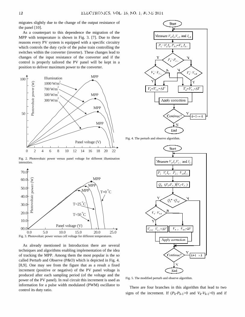
called Perturb and Observe (P&O) which is depicted in Fig. 4.

[8,9]. One may see from the figure that as a result a fixed

increment (positive or negative) of the PV panel voltage is

produced after each sampling period (of the voltage and the

power of the PV panel). In real circuit this increment is used as

information for a pulse width modulated (PWM) oscillator to

control its duty ratio.

Fig. 4. The perturb and observe algorithm.

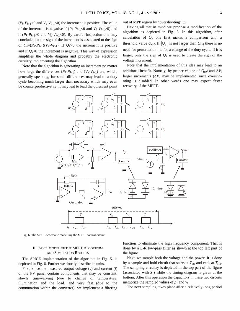
Fig. 5. The modified perturb and observe algorithm.

There are four branches in this algorithm that lead to two

signs of the increment. If (Pk-Pk-1>0 and Vk-Vk-1>0) and if

12 ELECTRONICS, VOL. 18, NO. 1, JUNE 2014

(Pk-Pk-1<0 and Vk-Vk-1<0) the increment is positive. The value

of the increment is negative if (Pk-Pk-1<0 and Vk-Vk-1>0) and

if (Pk-Pk-1>0 and Vk-Vk-1<0). By careful inspection one may

conclude that the sign of the increment is associated to the sign

of Qk=(Pk-Pk-1)(Vk-Vk-1). If Qk>0 the increment is positive

and if Qk<0 the increment is negative. This way of expression

simplifies the whole diagram and probably the electronic

circuitry implementing the algorithm.

Note that the algorithm is generating an increment no matter

how large the differences (Pk-Pk-1) and (Vk-Vk-1) are, which,

generally speaking, for small differences may lead to a duty

cycle becoming much larger than necessary which may even

be counterproductive i.e. it may leat to lead the quiescent point

out of MPP region by "overshooting" it.

Having all that in mind we propose a modification of the

algorithm as depicted in Fig. 5. In this algorithm, after

calculation of Qk one first makes a comparison with a

threshold value Qref. If kQ is not larger than Qref there is no

need for perturbation i.e. for a change of the duty cycle. If it is

larger, only the sign of Qk is used to create the sign of the

voltage increment.

Note that the implementation of this idea may lead to an

additional benefit. Namely, by proper choice of Qref and V,

larger increments (V) may be implemented since oversho-

oting is disabled. In other words one may expect faster

recovery of the MPPT.

Fig. 6. The SPICE schematic modelling the MPPT control circuit.

III. SPICE MODEL OF THE MPPT ALGORITHM

AND SIMULATION RESULTS

The SPICE implementation of the algorithm in Fig. 5. is

depicted in Fig. 6. Further we shortly describe its units.

First, since the measured output voltage (v) and current (i)

of the PV panel contain components that may be constant,

slowly time-varying (due to change of temperature,

illumination and the load) and very fast (due to the

commutation within the converter), we implement a filtering

function to eliminate the high frequency component. That is

done by a L-R low-pass filter as shown at the top left part of

the figure.

Next, we sample both the voltage and the power. It is done

by a sample and hold circuit that starts at Ts1s and ends at Ts1d.

The sampling circuitry is depicted in the top part of the figure

(associated with S1) while the timing diagram is given at the

bottom. After this operation the capacitors in these two circuits

memorize the sampled values of p1 and v1.

The next sampling takes place after a relatively long period

ELECTRONICS, VOL. 18, NO. 1, JUNE 2014 13

which is adjustable based on how fast changes of temperature

and illuminations are expected. Here the sampling instant

(associated with S2) is denoted by Ts2s. So after Ts2d we have

two new samples: p2 and v2.

Having these four quantities we compute Q=(p2-p1)(v2-v1)

which is represented in Fig. 6. as a controlled voltage source.

That signal is contrasted to Qref and the result is brought to a

limiter so that vq takes (approximately) values 0, 1V and -1V,

only.

The resulting vq is used to create the voltage increment at

Cx. It is vx=k∙vq∙t/Cx, where t=Ts3d-Ts3s. This increment is

brought to one of the inputs of a comparator. The second input

of the comparator is excited by the output (voltage) signal of

an oscillator that produces symmetrical alternatively linearly

rising and linearly falling signal. The oscillation period is

equal to the switching period of the converter so that at the

output of the limiter connected to the comparator`s output one

gets pulse width modulated signal.

After completion of the sampling at S3, using S4 the sampled

values of v1, v2, p1, and p2, are erased and a new measurement

and control cycle is enabled. Here, to shorten the computer

time, a measurement/control period of 100 ms was used. In

real world that interval is supposed to be longer.

The following set of parameter values was used to enable

the simulation of the circuit in Fig. 6: a=1, r=1Ω, C=1µF,

L=1H, R=1kΩ, Qref=0.5V, Rs=10kΩ, Cs=0.9nF, k=10-3

,

Cx=14.3mF, Ts1s=5ms, Ts1d=10ms, Ts2s=70ms, Ts2d=75ms,

Ts3s=85ms, Ts3d=90ms, Ts4s=95ms, Ts4d=100ms. No battery was

included in the system.

To illustrate the implementation of the algorithm an

example will be shown. Instead of getting the signals directly

from the PV panel, for verification purposes, we created two

signals as follows (Figs. 7 and 8):

v(t)=2+ sin(2π·50000·t)+sin(2π·0.5·t) [V] (1a)

i(t)=0.6+sin(2π·50000·t)+sin(2π·0.5·t+/2) [A]. (1b)

Fig. 7. Input voltage signal.

Fig. 8. Input current signal.

These were used as excitation for the circuit in Fig. 6. Fig.

9. depicts the signal Q of Fig. 6. Finally, Fig. 10 illustrates the

dependence of the duty cycle at the output of the circuit in Fig.

6. It is clear that it follows the shape of Q. It also implements

the new version of the MPPT algorithm presented in Fig. 5.

Fig. 9. The Q=(p2-p1)(v1-v2) product.

In Figs. 11 and 12 pulses at the circuit output are given for

two different time instances. We can see that pulse width

dramatically changes in time, which was in fact the goal.

Fig. 10. Dependence of the duty cycle at the output of the circuit of Fig. 6.

14 ELECTRONICS, VOL. 18, NO. 1, JUNE 2014

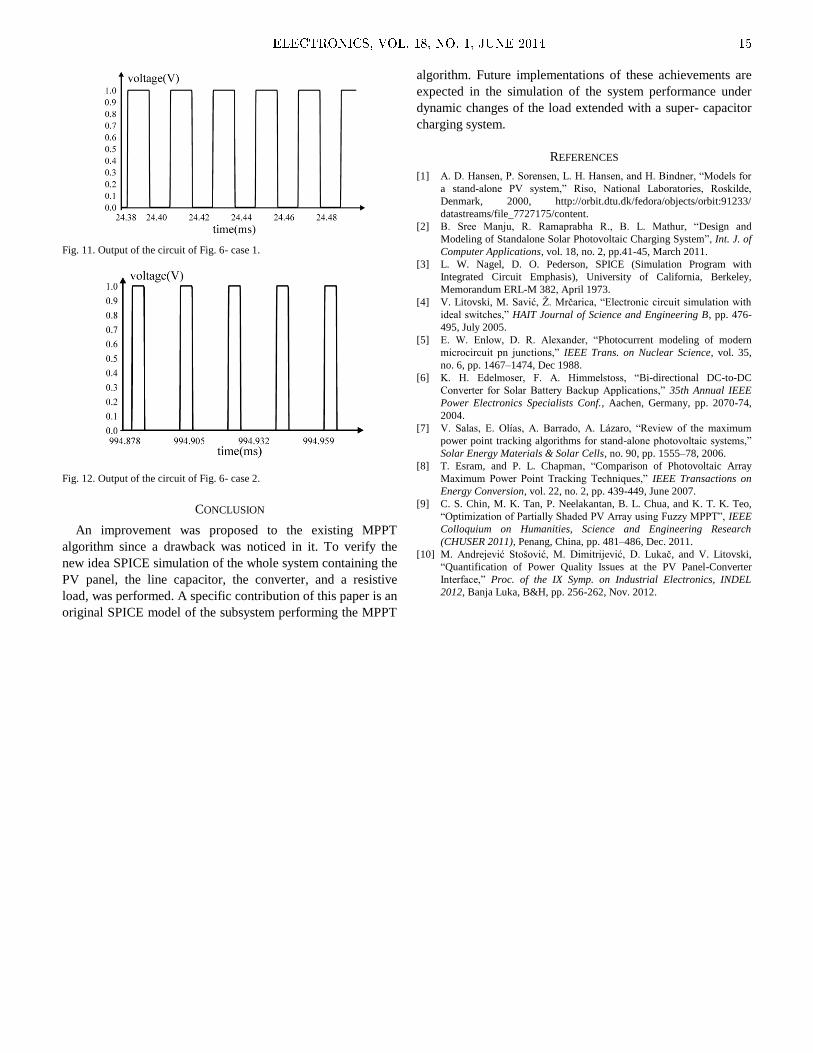
Fig. 11. Output of the circuit of Fig. 6- case 1.

Fig. 12. Output of the circuit of Fig. 6- case 2.

CONCLUSION

An improvement was proposed to the existing MPPT

algorithm since a drawback was noticed in it. To verify the

new idea SPICE simulation of the whole system containing the

PV panel, the line capacitor, the converter, and a resistive

load, was performed. A specific contribution of this paper is an

original SPICE model of the subsystem performing the MPPT

algorithm. Future implementations of these achievements are

expected in the simulation of the system performance under

dynamic changes of the load extended with a super- capacitor

charging system.

REFERENCES

[1] A. D. Hansen, P. Sorensen, L. H. Hansen, and H. Bindner, “Models for

a stand-alone PV system,” Riso, National Laboratories, Roskilde,

Denmark, 2000, http://orbit.dtu.dk/fedora/objects/orbit:91233/

datastreams/file_7727175/content.

[2] B. Sree Manju, R. Ramaprabha R., B. L. Mathur, “Design and

Modeling of Standalone Solar Photovoltaic Charging System”, Int. J. of

Computer Applications, vol. 18, no. 2, pp.41-45, March 2011.

[3] L. W. Nagel, D. O. Pederson, SPICE (Simulation Program with

Integrated Circuit Emphasis), University of California, Berkeley,

Memorandum ERL-M 382, April 1973.

[4] V. Litovski, M. Savić, Ž. Mrčarica, “Electronic circuit simulation with

ideal switches,” HAIT Journal of Science and Engineering B, pp. 476-

495, July 2005.

[5] E. W. Enlow, D. R. Alexander, “Photocurrent modeling of modern

microcircuit pn junctions,” IEEE Trans. on Nuclear Science, vol. 35,

no. 6, pp. 1467–1474, Dec 1988.

[6] K. H. Edelmoser, F. A. Himmelstoss, “Bi-directional DC-to-DC

Converter for Solar Battery Backup Applications,” 35th Annual IEEE

Power Electronics Specialists Conf., Aachen, Germany, pp. 2070-74,

2004.

[7] V. Salas, E. Olías, A. Barrado, A. Lázaro, “Review of the maximum

power point tracking algorithms for stand-alone photovoltaic systems,”

Solar Energy Materials & Solar Cells, no. 90, pp. 1555–78, 2006.

[8] T. Esram, and P. L. Chapman, “Comparison of Photovoltaic Array

Maximum Power Point Tracking Techniques,” IEEE Transactions on

Energy Conversion, vol. 22, no. 2, pp. 439-449, June 2007.

[9] C. S. Chin, M. K. Tan, P. Neelakantan, B. L. Chua, and K. T. K. Teo,

“Optimization of Partially Shaded PV Array using Fuzzy MPPT”, IEEE

Colloquium on Humanities, Science and Engineering Research

(CHUSER 2011), Penang, China, pp. 481–486, Dec. 2011.

[10] M. Andrejević Stošović, M. Dimitrijević, D. Lukač, and V. Litovski,

“Quantification of Power Quality Issues at the PV Panel-Converter

Interface,” Proc. of the IX Symp. on Industrial Electronics, INDEL

2012, Banja Luka, B&H, pp. 256-262, Nov. 2012.

ELECTRONICS, VOL. 18, NO. 1, JUNE 2014 15

Abstract—The main objective of this paper is to present a new

method of predictive maintenance which can detect the states of

coal grinding mills in thermal power plants using Bayesian

networks. Several possible structures of Bayesian networks are

proposed for solving this problem and one of them is implemented

and tested on an actual system. This method uses acoustic signals

and statistical signal pre-processing tools to compute the inputs of

the Bayesian network. After that the network is trained and

tested using signals measured in the vicinity of the mill in the

period of 2 months. The goal of this algorithm is to increase the

efficiency of the coal grinding process and reduce the

maintenance cost by eliminating the unnecessary maintenance

checks of the system

Index Terms—Acoustic Signals, Bayesian Networks, Predictive

Maintenance, Ventilation Mills.

Original Research Paper

DOI: 10.7251/ELS1418016V

I. INTRODUCTION

ONDITION based maintenance (CBM) is a maintenance

technique widely used in the industry today. It uses data

collected through condition monitoring to advise whether

maintenance is necessary, and thus reduces maintenance cost

of the system [1]. Many of the maintenance techniques that are

currently implemented are using a certain type of time-based

preventive maintenance, where the components of the system

are checked regularly after a certain period of time to ensure

that no serious fault has occurred. This kind of maintenance is

being conducted on ventilation mills in thermal power plants

where, due to the inability to predict the state of the coal

grinding plate within the mill, the entire subsystem needs to be

periodically stopped and inspected. This paper proposes a new

method of predictive maintenance which can detect the state of

the plates within the mills based on the acoustic signals

Manuscript received 13 April 2014. Accepted for publication 30 May

2014.

S. Vujnović is with the School of Electrical Engineering, University of

Belgrade, Belgrade, Serbia (phone: +381-11-3218-370; e-mail:

svujnovic@etf.bg.ac.rs).

P. Todorov is with the School of Electrical Engineering, University of

Belgrade, Belgrade, Serbia (e-mail: pedjatodorov@etf.bg.ac.rs).

Ž. Đurović is with the School of Electrical Engineering, University of

Belgrade, Belgrade, Serbia (e-mail: zdjurovic@etf.bg.ac.rs).

A. Marjanović is with the School of Electrical Engineering, University of

Belgrade, Belgrade, Serbia (e-mail: amarjanovic@etf.bg.ac.rs).

measured in the vicinity of the mill, using Bayesian networks

(BN).

Bayesian networks have been widely used for the purpose of

predictive maintenance in the last few years. Since their

introduction in the mid 80’s [2] they have experienced a rapid

development in many areas of research. Also, due to their

ability to represent complex systems in which high amount of

uncertainty exists, they have proven themselves to be superior

to other methods such as neural networks, support vector

machines, etc. In this paper several BN structures will be

proposed which serve to model the states and the behaviors of

ventilation mills, and one of them will be tested on actual

acoustic measurements.

There are many examples of fault detection algorithms

which are based on the measurements of vibration signals of

the machines ([3] and [4], to name a few). However, it has

long since been shown that acoustic measurements can be as

informative as vibration signals when it comes to detecting the

faults in machines [5]. The usage of acoustic signals in fault

detection has expanded during the last decade [6], however

they are still considered to be a lesser alternative to vibration

signals, due to their high susceptibility to surrounding noise. In

this paper acoustic signals acquired in a very noisy

environment will be used to test the efficiency of a simple

Bayesian network for the detection of states in the ventilation

mills. More complex realizations of the solution to the

problem will be proposed as well.

This paper is structured as follows. In Chapter 2 a short

introduction to Bayesian Networks is presented, while in

Chapter 3 some practical realizations of BNs which can be

used for fault detection are proposed. Chapter 4 describes the

system on which the algorithms have been tested, as well as

the process of acquiring acoustic signals. In Chapter 5 the

results of the algorithm are presented and in Chapter 6 the final

conclusions to this paper are stated.

II. BAYESIAN BELIEF NETWORKS

Bayesian Belief Network (BBN) is a term introduced in

1980s by Jude Pearl [2] in an attempt to create a mathematical

probabilistic tool capable of modeling and reproducing the

process of human reasoning. The basic idea was to reproduce

the way in which people accumulate information from

different sources and use it to develop conclusions about

certain ideas. During the last decade Bayesian networks have

become a very powerful tool for representation of complex

The use of Bayesian Networks in Detecting the

States of Ventilation Mills in Power Plants

Sanja Vujnović, Predrag Todorov, Željko Đurović, and Aleksandra Marjanović

C

16 ELECTRONICS, VOL. 18, NO. 1, JUNE 2014

systems and it has been used in many areas of research

including fault detection and fault isolation [7], [8].

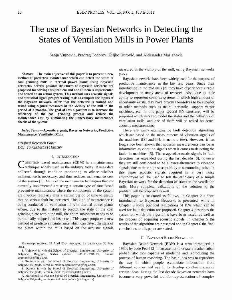
Fig. 1. A simple Bayesian network which consists of 4 nodes (X1, X2, X3 and

X4) and three connections between them.

A. Bayesian Theorem

Bayesian networks apply Bayesian theorem on complex

systems to calculate conditional probabilities of certain events

or hypothesis when a new evidence is obtained. Bayesian

theorem was coined by Thomas Bayes in the 18th century and

it can be formulated as

.)(

)|()()|(

EP

HEPHPEHP nn

n (1)

Here ( | )nP H E is a posterior probability of hypothesis

Hn when evidence E is known. ( )nP H and ( )P E are prior

probabilities of hypothesis and evidence, respectively, and

( | )nP E H is the probability of evidence E given the

hypothesis nH . The great advantage of Bayes' theorem is that

it allows us to easily calculate conditional probabilities based

on the corresponding prior probabilities. In this case, if nH is,

for example, a certain fault, and E is evidence or a symptom

of a fault, than ( )nP H and ( | )nP E H can be more easily

obtained from the survey or maintenance data, than the

conditional probability of a fault given the evidence.

If we assume that i denotes a specific hypothesis iH , then

(1) can be rewritten using the rule of total probability, where

the summation is taken over all hypotheses iH which are

mutually exclusive and their prior probabilities sum up to 1.

The final form is given as

.)|()(

)|()()|(

i ii

nn

nHEPHP

HEPHPEHP (2)

This is called inference and it represents the basic idea of

how the inserted evidence spreads throughout Bayesian

networks.

B. Topology of Bayesian Network

Bayesian network is an acyclic probabilistic graph which

contains a set of nodes and directed connections between them

and it is used to represent the knowledge about uncertain

events. Nods represent the probabilistic variables which can be

continuous or discrete. Connections between nodes represent

the probabilistic dependencies among certain variables. A

simple type of Bayesian network is shown in Fig. 1. Here an

edge from node X1 to node X3 and from nodes X1 and X2 to

node X4 represent a statistical dependence between the

corresponding variables. Therefore a value taken by a variable

X4 depends on the values taken by variables X1 and X2. Nodes

X1 and X2 are then referred to as the parents of X4 and,

similarly, X4 is referred to as the child of X1 and X2. In general,

for the network with n nodes: X1, X2,..., Xn, the joint

probability can be expressed as

1 2

1

( , ,..., ) ( | ( )) ,n

n i i

i

P X X X P X pa X

(3)

where ( )ipa X is a set of parents of the node iX .

There are many types of nodes which can be chosen for any

given Bayesian network. However, in practice only two types

of variables are used: discrete and continuous Gaussian. This

is because only for these two types of nodes can the exact

computation of conditional probabilities be done [9].

Similarly, the discrete variables cannot have continuous

parents if the exact computation is required. Therefore, there

are three different combinations of nodes for the parent-child

relationship and three different methods for calculating

conditional probabilities. If discrete variables have discrete

parents, their conditional probabilities are expressed via

conditional probability table. For example, if both X1 and X3

from Fig. 1 are discrete variables, with n and m different

possible states respectively, their conditional probability table

would have n x m entries of conditional probabilities

3 3 1 1( | )i kP X x X x , where 3ix is the i-th state of node X3

and 1kx the k-th state of the node X1. On the other hand, if X3

was a Gaussian continuous variable and X1 its discrete parent,

the conditional probability distribution would be Gaussian as

well [9].

C. The Learning Process

There are two ways of calculating parameters of Bayesian

network, as well as the structure. One is based on an expert

knowledge of the system and the other on machine learning

using experimental results. These two approaches can be used

jointly or individually.

Assuming that the expert knowledge of the system is

unavailable and that Bayesian network needs to be taught its

structure and parameters, there are several ways in which this

can be achieved. Structure learning itself is much more

complicated than the parameter learning and we will not dwell

on it further in this paper. For all intents and purposes we will

assume that the structure of the Bayesian network is known

and that only the parameters need to be taught.

In the case when all the nodes (variables) of the system are

observable, the most common algorithm for machine learning

of the Bayesian network is the log likelihood approach. Here

ELECTRONICS, VOL. 18, NO. 1, JUNE 2014 17

the goal is to learn all of the conditional probability densities

which maximize the likelihood of the training data. That is to

Fig. 2. Bayesian network with one measured continuous node (X3), one

hidden discrete node (X2) and one discrete node which represents the state of

impact plates and which cannot be directly measured (X1).

say that if we have Bayesian network ( , )B S p with defined

structure S and parameters p, and where D is a set of training

data with the values of all the parameters p of network B, then

the goal is to maximize the likelihood, i.e. the probability of

the data d given the Bayesian network B:

( | ) ,d D

L P d B

(4)

or as it is more commonly expressed in logarithmic form:

.)|(log 2

Dd

BdPLL (5)

If by any chance there is a choice of several Bayesian

network models, it is wise to adopt the model which gives the

maximum likelihood given the data obtained.

Usually however, not all the parameters can be measured,

and some connections between the nodes must be modeled

with unobservable variables. In such cases the exact log

likelihood approach cannot be used and the approximate

parameter estimation must be conducted. The most popular

approximate algorithm for teaching the Bayesian network with

hidden nodes is the Expectations maximization (EM)

algorithm. This algorithm consists of two steps. In the first

step, called the expectation step, the current parameter

estimations p are used to calculate expectations for the

missing values of hidden variables. Then, in the second step

called the maximization step, a new maximum likelihood

estimate of the parameters is calculated after which the

algorithm goes back to the previous step. This continues

throughout the entire training set.

III. APPLICATION OF BAYESIAN NETWORK IN PREDICTIVE

MAINTENANCE

The fundamental problem with Bayesian networks is

deciding which model adequately represents the system which

is observed. First of all, the variables used in the system need

to be chosen. They can represent some physical, measurable

property of the system or some unknown interference which

Fig. 3. Hidden Markov model represented with Bayesian networks. Xi

S are the

states of the system and XiM are the measurements of the system. All the

variables are continuous Gaussian and visible.

cannot be measured. Then, the decision needs to be made

concerning the type of the chosen variables. They can be

discrete or continuous, visible or hidden. Secondly, the

question of the structure of the Bayesian network should be

decided upon. This is the most important and the most

complex question. The types of structures which can be

represented with Bayesian networks are vast, and the only

limit one faces when choosing them is the knowledge of the

causal relationships within the physical system and the

complexity sufficient to solve the given problem. In this

chapter several structures will be proposed for solving the

problem of detecting the states of ventilation mills.

A. The Simple Static Model

The simplest Bayesian network that can be used for

detecting the state of the mill is shown in Fig. 1. Circles

represent continuous-valued random variables, squares are

discrete random variables, clear boxes represent observed

nodes and gray boxes represent hidden nodes. This network

contains only 3 nodes (variables), two of which are discrete

and one of which is continuous Gaussian.

The basic idea is that the measurements taken outside of the

mill are directly influenced by the state of the impact plates

within the mill and by a hidden variable which is modeled as a

discrete node. This hidden, immeasurable node can represent

an outside noise, unknown component of the system or some

other feature which does not necessarily need to have a

physical interpretation. The state of the plates X1 is modeled as

a discrete node with 2 states: healthy plates and worn plates.

The measured signal which is represented by the node X3 is a

two-dimensional Gaussian variable.

B. Hidden Markov Model

Hidden Markov model (HMM) can be modeled as a simple

dynamic Bayesian network, where the next state of the system

depends on the previous state and the state transition

probabilities, and where the states themselves are not directly

measured. However, even though the states cannot be

18 ELECTRONICS, VOL. 18, NO. 1, JUNE 2014

Fig. 4. Complex dynamical BN model. Xi

S are the states of the system, XiM are the measurements of the system and Xi

H. are the hidden variables of the system

which cannot be observed or detected. All the nodes are continuous and Gaussian.

measured, they influence the measurements of the system

which are then used to infer the state in which the system is in.

Hidden Markov models are used for a very broad range of

systems and one such model (Fig. 3) can be used to infer the

states of the impact plates in ventilation mills.

In Fig. 3, XiS represents a state node and Xi

M a measurement

node. All of the variables are chosen to be continuous and

visible (that is to say, information on states and measurements

can be used when training the network). In this case 3

continuous states are chosen: the state of healthy plates (X1S ),

the state when the plates are used but not damaged enough, so

the repair is not necessary (X2S ) and the state which represents

worn plates (X3S ) and which indicates that the repair should be

done as soon as possible.

Note that the transition between states is modeled so that the

state deteriorates up until a point when the plates have to be

replaced, and only then can the state return to the initial value

of healthy plates. Also, each state influences the appropriate

measurement of the system, but due to noise and

inconsistencies it can appear as a measurement of the adjacent

state as well (presented by dotted lines in Fig. 3).

A. The Complex Dynamical Model

As we have noted, HMM are broadly used to model all sorts

of systems in many areas of research. However, they represent

only a simple usage of dynamic Bayesian network which can

easily be modified to include more complex demands of the

system. One such modification is proposed in Fig 4, where the

mixture of first two solutions to Bayesian network models is

implemented. Here the one-way transition between the states is

included as well as the influence of the unknown, hidden

variable on the measurements of the system.

IV. CASE STUDY

In the previous chapter some possible structures of Bayesian

networks were proposed that can be used for predictive

maintenance. The actual process on which one of these

solutions will be tested is a ventilation mill in thermal power

plant Kostolac A (Serbia) and it will be described in this

chapter. Also, the process of acquiring and pre-processing of

acoustic signals used in simulations will be depicted.

A. Ventilation Mill

Coal grinding mills are a very important subsystem of

thermal power plants. Their main purpose is to pulverize the

coal into fine powder before it can get into the furnace. The

mill itself consists of coal grinding plates (also called impact

plates) which rotate within it with the frequency of fr=12.5Hz

and are used to crush the coal into smaller pieces until it gets

sufficiently fragmented. After that it drifts into the furnace

system where it is used as a fuel.

During the grinding process the impact plates get slowly

depleted and their efficiency reduces. In the early stages this

causes them to pulverize the coal more slowly, but if the plates

are not changed for a long period of time it can cause a

complete malfunction of the milling subsystem in thermal

power plants. Some algorithms for solving this problem have

already been proposed [10]. Currently this problem is being

solved by employing a type of time based maintenance, which

implies stopping the entire subsystem once every 8 or 9 weeks,

conducting visual inspection of the plates and, if it is deemed

necessary, replacement of the plates with the new ones. This

can be very costly if the overhaul was concluded not to be

necessary.

In this paper a new algorithm will be tested which uses

acoustic signals recorded in the vicinity of the mill, while the

mill is operating mode, and Bayesian networks to determine

the state of the impact plates, i.e. whether the replacement is

necessary or not.

B. Acoustic Signals

Acoustic signals were recorded in the vicinity of the mill

while it was in operating mode. The measurements were

conducted every couple of weeks in the period of two months,

thus encompassing the entire life cycle of the plates, from the

moment they were replaced to the moment when they were

completely depleted. These signals were recorded with the

ELECTRONICS, VOL. 18, NO. 1, JUNE 2014 19

sampling frequency of fs=48kHz and 24bit encryption.

Approximately once every two weeks an acoustic signal has

been measured, which has afterward been divided into 20-30

shorter signals.

For the training and testing of the Bayesian network the

sampling period was downsized to 4.8kHz, Also, certain

features were extracted from the signal which were later used

in the decision making process. These features are the basic

properties of the signal in time and frequency domain. Eight

features in time domain are chosen as characteristic parameters

of the signal [3]:

Arithmetic mean value:1

1( )

N

ix x i

N

Root mean square value: 1/2

2

1

1( )

N

rms ix x i

N

Square mean root value: 2

1/2

1

1( )

N

r ix x i

N

Skewness index: 3 3/2

1

1( ) /

N

ske vix x i x x

N

Kurtosis index: 2

1

1( ) 4 /

N

kur vix x i x x

N

C factor: / rmsC PP x

L factor: / rL PP x

S factor: /rmsS x x

where xv is the variance of the signal x and PP is peak-to-peak

value of the signal. Also, eight features in the frequency

domain were chosen as the most dominant components in the

frequency spectrum of the signal, in the same way it has been

done in [10]. They represent the maximum value of the

amplitude frequency spectrum of the signal at the frequencies:

25 37.5 50 62.5 125 250 375 500f Hz.

After extracting these features a vector of 16 elements is

acquired for each of the measured signals. To reduce the

dimension of this vector and therefore reduce the amount of

variables needed for the Bayesian network, a linear dimension

reduction algorithm is applied which transforms a 16-

dimentional vector X into a two-dimentional vector Y [11]:

.1221612 x

T

xx XAY (6)

The matrix A is chosen so to minimize the loss of

information by maximizing the distance of two extreme classes

- the class of healthy and the class of worn plates. This matrix

is acquired by maximizing the criteria 1

( )W B

J tr S S

where

WS is a within-class scatter matrix and

BS is a between-class

scatter matrix, as defined in [11], and applied in [3]. After this

procedure has been implemented, the 2-dimensional vector of

features Y is used as an input to a Bayesian network.

V. RESULTS

For the testing of this algorithm the Bayesian Network

depicted in Fig. 2 is used. The first variable (X1) represents the

true state of the system and is chosen to be a discrete variable

with two possible states - healthy and worn plates. The second

variable (X2) is a hidden variable and it does not have a

specific physical meaning. It represents the noise in the

surroundings that can influence the measurements, as well as

unknown parameters of the system that were not otherwise

included in the model. It is also chosen to be a discrete

variable with two possible states. Finally, the third variable

(X3) represents the measured output of the system, or in this

case, a parameter Y gained by signal pre-processing techniques

described in the previous chapter. This variable is chosen to be

continuous and Gaussian. With this in mind, the joint

probability of this Bayesian network is:

.)()|(),|(),,( 112213321 XPXXPXXXPXXXP (7)

The idea is to calculate the probability of each of the states

in X1 given the measurements X3.

Learning and testing procedures for this Bayesian network

are done in a programming package Matlab, using toolbox for

Bayesian networks created by [9]. For a training set, the

signals taken slightly before and slightly after the change of

plates were chosen, representing the two extreme states of the

mill. Since there is a hidden node within the system, the EM

learning algorithm is applied. The testing is done on all the

signals. No initial assumptions about the conditional

probabilities were made, so only after the learning process has

been completed, the conditional probability table for all the

nodes had been constructed. The testing has been done in two

ways - real time and offline testing.

In average of every two weeks, a recording has been

conducted, enabling us to acquire around 30 acoustic signals,

thus giving us a complete database of a over 120 signals

throughout the entire lifespan of the grinding plates. In order

to test this algorithm in real time, all these signals have been

artificially merged so to appear as though the seconds have

passed between different measurement sessions, when indeed

it has actually been weeks. However, despite the artificially

created sudden changes in the state of the mill (which are

realistically much slower) the algorithm tested in real-time has

shown some very good results.

From Fig. 5 it can be concluded that this simple Bayesian

network can successfully detect the states of the grinding

plates. Two weeks after they have been changed the algorithm

detects that the plates are completely healthy, 5 weeks after the

change the deterioration of the plates becomes noticeable, and

the Bayesian network detects 25% probability that the plates

are worn. After 6 weeks this percentage increases to 50%,

whereas after 8 weeks the algorithm reports with 100%

certainty that the plates need to be replaced. In order to

prevent sudden changes in real time testing environment, the

output of the Bayesian network is averaged over the last 10

time periods (each of which lasts 15 seconds). It can be noted

20 ELECTRONICS, VOL. 18, NO. 1, JUNE 2014

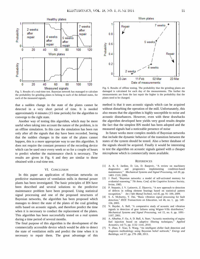
Fig. 5. Results of a real-time test. Bayesian network has managed to calculate

the probability for grinding plates to belong to each of the defined states, for

each of the measured signals.

that a sudden change in the state of the plates cannot be

detected in a very short period of time. It is needed

approximately 4 minutes (15 time periods) for the algorithm to

converge to the right state.

Another way of testing this algorithm, which may be more

useful when taking into account the nature of the problem, is in

an offline simulation. In this case the simulation has been run

only after all the signals that day have been recorded. Seeing

that the sudden changes in the state of the plates cannot

happen, this is a more appropriate way to use this algorithm. It

does not require the constant presence of the recording device

which can be used once every week or so for a couple of hours

to predict whether the maintenance check is necessary. The

results are given in Fig. 6 and they are similar to those

obtained with a real-time test.

VI. CONCLUSION

In this paper an application of Bayesian networks on

predictive maintenance of ventilation mills in thermal power

plants has been investigated. The basic principles of BN have

been described and several solutions to the predictive

maintenance problem have been proposed. Using statistical

signal processing and one of the proposed structures of

Bayesian networks, the algorithm has been proposed which

manages to detect the state of the plates of the coal grinding

mills based on acoustic signals, and therefore predict the time

when it is necessary to conduct the replacement of the plates.

This algorithm has been successfully tested on a real system

during a time period of several months.

The final purpose of this algorithm is the development of the

commercially accessible device which would be able to detect

the state of ventilation mills and predict the time when it is

necessary to repair them. The great advantage of this

Fig. 6. Results of offline testing. The probability that the grinding plates are

damaged is calculated for each day of the measurements. The further the

measurements are from the last repair the higher is the probability that the

plates need to be changed.

method is that it uses acoustic signals which can be acquired

without disturbing the operation of the mill. Unfortunately, this

also means that the algorithm is highly susceptible to noise and

acoustic disturbances. However, even with these drawbacks

the algorithm developed here yields very good results despite

the fact that the simplest BN model has been adopted and the

measured signals had a noticeable presence of noise

In future works more complex models of Bayesian networks

that include the dynamic behavior of the transition between the

states of the system should be tested. Also a better database of

the signals should be acquired. Finally it would be interesting

to test the algorithm on acoustic signals gained with a cheaper

microphone which is commercially more available.

REFERENCES

[1] A. K. S. Jardine, D. Lin, D. Banjevic, “A review on machinery

diagnostics and prognostics implementing condition-based

maintenance,” Mechanical Systems and Signal Processing, vol 20, pp.

1483–1510, 2006.

[2] J. Pearl, “Bayesian networks: a model of self-activated memory for

evidential reasoning,” 7th Annu. Conf. of the Cognitive Science Society,

Irvine, 1985.

[3] P. Stepanic, I. V. Latinovic, Z. Djurovic, “A new approach to detection

of defects in rolling element bearings based on statistical pattern

recognition,” Int J Adv Manuf Technol, vol 45, pp. 91–100, 2009.

[4] S. A. McInerny, Y. Dai, “Basic vibration signal processing for fault

detection,” IEEE Transactions on Education, vol 46, no. 1, pp. 149–

156, 2003.

[5] N. Baydar, A. Ball, “A comparative study of acoustic and vibration

signals in detection of gear failures using Wigner-Ville distribution,”

Mechanical Systems and Signal Processing, vol 15, no. 6. pp. 1091–

1107, 2001.

[6] A. Albarbar, F. Gu, A. D. Ball, A. Starr, “Acoustic monitoring of engine

fuel injection based on adaptive filtering techniques,” Applied

Acoustics, vol 71, pp. 1132–1141, 2010.

[7] Y. Zhao, F. Xiao, S. Wang, “An intelligent chiller fault detection and

diagnosis methodology using Bayesian belief nettwork,” Energy and

Buildings, vol 57, pp. 278–288, 2013.

ELECTRONICS, VOL. 18, NO. 1, JUNE 2014 21

[8] S. Verron, J. Li, T. Tiplica, “Fault detection and isolation of faults in a

multivariate process with Bayesian network,” Journal of Process

Control, vol 20, pp. 902–911, 2010.

[9] K. P. Murphy, “Dynamic Bayesian networks: Representation, Inference

and Learning,” Ph.D. dissertation, Dept. Computer Science, Univ. of

California, Berkeley, 2002.

[10] E. Kisić, V. Petrović, S. Vujnović, Ž. Đurović, M. Ivezić, “Analysis of

the condition of coal grinding mills in thermal power plants based on

the T2 multivatiate control chart applied on acoustic measurements,”

Facta Universitatis Series: Automatic Control and Robotics, vol 11, no.

2, pp. 141–151, 2012.

[11] K. Fukunaga, Introduction to Statistical Pattern Recognition. Boston:

Academic Press, 1980.

22 ELECTRONICS, VOL. 18, NO. 1, JUNE 2014

Abstract—This paper describes a new verification environment

for USB 2.0 controller. New methodology is presented, where a

co-simulation environment is used as one of the starting points for

the embedded hardware/software development and as an

accelerator of the overall design process. The verification

environment is based on the device emulation/virtualization

technique, using USB controller’s real register transfer level

(RTL) instead of models. This approach is functionally very close

to the corresponding real-world devices and allows wider

opportunities for hardware debugging. The new software utilities

for USB host and device functionality testing are also presented.

This tool allows generating custom tests by including various

transfer types and modifying parameters such as data payload,

interval, number of pipes, etc. It can be used for both hardware

(HW) and software (SW) limitations characterization, as well as

debugging.

Index Terms—Co-simulation, FPGA, System C, QEMU, USB

Original Research Paper

DOI: 10.7251/ELS1418023G

I. INTRODUCTION

HE Universal Serial Bus (USB) is a fast, bidirectional,

low-cost, dynamically attachable communication interface

consistent with the requirements of the present microelectronic

platforms [1]. It is widely used in the huge number of

instruments and devices, which include personal computers,

digital cameras, scanners, image devices, printers, keyboards,

mice, telephones, embedded systems, systems on a chip (SoC),

etc. Fig. 1 shows the high-level architecture diagram of USB

controller within a typical system.

Field programmable gate array (FPGA) based techniques

can be used for verification and functional debuging in design

flow of USB IPs. In this approach, hardware core is mapped

onto an emulation platform, based on an FPGA that mimics

the behavior of the final chip, and the software modules are

loaded into the memory of the emulation platform. Once

programmed, the emulation platform enables testing and

debugging of hardware (HW) and software (SW) components,

close to system’s full operational speed. In fact, FPGAs are

used primarily to speed up testing and make some parts of the

verification easier. Various components of USB system can be

Manuscript received 13 April 2014. Accepted for publication 30 May

2014.

G. Y. Zargaryan, V. K. Aharonyan, N. V. Melikyan are with the Synopsys

Armenia CJSC (e-mail: grigorz, vahrama, nazeli@synopsys.com ).

M. A. Dimitrijević is with Faculty of Electrical Engineering, University of

Niš, Niš, Serbia, (+381-18-529-321; e-mail: marko@venus.elfak.ni.ac.rs).

prototyped and verified using FPGAs. In [2] the development

of USB peripheral core on the FPGA is described. USB

protocol analyzer and the core were implemented for

verification. For example, only UTMI logic can be designed

using VHDL code, then simulated, synthesized and

programmed to the targeted FPGA [3]. But the drawback of

both approaches [2], [3] is that designed components were not

fully validated in complete USB system (including host, USB

SW stack, etc.).

USB 3.0

controller

ULPI PHY

PIPE PHY

ULPI

PIPE

Ap

pli

cati

on

Bu

s

Master

Slave I/F

SSRAM

Dat

a F

IFO

RA

M I

/F

CPU

Memo

Peripheral 1

Peripheral 2

Interrupt

Another drawback of FPGA based HW verification can be

relatively slow debugging of signals, when some problem in

register transfer level (RTL) emerges. If the developer wants

to look at some signals generated in the core, he needs to

perform some modifications in RTL, connect appropriate

wires to the debug pins of chip, resynthesize logic, connect

analyzing osciloscope tools like Logic Analyzer and trigger the

signals or use JTAG cable to connect to FPGA and store

necessary signals in RAM memory supported (which requires

more resources) and finaly study signals from this store point.

If the developer is trying to proceed directly with RTL

validation in real system using FPGAs, problems can occur

with the absence of other USB system’s components (USB

PHY chip, programmable processor of SoC, memory access

unit, etc.).

On the other hand, in order to actually validate and use the

implemented USB hardware in applications running by SoC or

some other system, the software layer that encapsulates the

underlying hardware and provides the application developer

defined API (at minimum it is the so called hardware driver or

the hardware abstraction layer; often it contains more software

layers like OS modules) should be developed. Thus, only

hardware subcomponents (in this case USB IP core licensed

by suppliers) become a combination of hardware and software.

USB HW/SW Co-Simulation Environment with

Custom Test Tool Integration Zargaryan Y. Grigor, Aharonyan K. Vahram, Melikyan V. Nazeli and Marko A. Dimitrijević

T Fig.1. System-Level Block diagram including USB controller.

ELECTRONICS, VOL. 18, NO. 1, JUNE 2014 23

In this case, bare USB hardware IP is not enough.

Development of this software usually starts when the hardware

part is finished (or almost finished) and can be prototyped in

an FPGA device. This may considerably extend the project

timeframe. Early software development based on virtual

prototyping is getting more popular at system level, but in the

IP development it has not become a common practice yet. To

overcome the above mentioned problems, the necessity arises

to have a complete emulation and simulation environment for

USB coreduring controller design flow, .

II. BACKGROUND OF KNOWN METHODS FOR SIMULATION AND

VALIDATION OF USB CONTROLLER

SystemC [4], [5] has solved many of the software-hardware

co-simulation issues today, and software based verification

perfectly supports the new IP packaging requirements (i.e.

requirement to deliver hardware dependent software along

with the hardware component). Therefore, to design a USB

controller HW in a faster manner and to begin the

development of necessary drivers in the first stage of the

design, various modeling and verification methods have been

suggested. In [6] USB device simulation using Microsoft

Device Simulation Framework (DSF) is presented, which

allows quick construction of a virtual mass storage USB

device having final RTL architecture, but DSF does not

provide sufficient capabilities for USB simulation and

validation, and offers only smoke tests (i.e. file copy from and

to). Paper [7] describes the way of simulation and validation

system design for USB peripheral device’s Verilog HDL code

using SmartModel tools which include functions of USB 2.0

host and UTMI. This environment tests main functions of

device peripheral without SW stack (Start of Frame packet

generation, handling of Split transfers, ping protocol, etc.).

Paper [8] presents the USB host controller verification

environment using Transaction Level modeling (TLM), but

this environment actually does not cooperate with RTL, nor

USB host software, delivered as the final package to the user.

Only in [9] an example is given of design flow that includes

real HW (described in RTL language) validation with SW

stack. Here, SystemC TLM is used for hardware architecture

definition and preliminary SW development, in the first step.

RTL verification and prototyping is the next step. User-level

test is done only after USB RTL prototyping to the FPGA.

In this paper, a new approach to HW/SW co-simulation and

verification technique is proposed, using two entries of USB

Super-Speed (SS) core acting as a host and device. It allows

testing and validation of Verilog HDL code of USB core

together with depending software (SW) drivers, whole Linux

USB stack, running real user level applications (for either

smoke or stress tests, or specific protocol testing means [10]),

which makes simulation very close to real testing and

debugging. The main role of the simulation environment is to

make the USB controller work in real physical world

conditions prior to implementation on FPGA or ASIC. The

USB host and device controllers are attached to the emulated

x86 PCs running 3.6.3 Linux kernel using PCI bus. The

simulation environment provides full access to all signals of

RTL, during and after simulation. The possibility of capturing

and analyzing data packets sent and received over USB bus is

also provided. PC systems are emulated using QEMU open

source virtualization software which works straightforwardly

with verification environment, considering it as a combination

of two real-world Linux systems connected to each other via

USB. Another important advantage of this method is that the

other USB controller (EHCI, OHCI, USB 3.0 xHCI) RTL

codes can be easily integrated into verification environment as

well, after specific changes in Verilog source code of USB

PHY model. As Linux OS runs on emulated PC, the validation

of these controllers with corresponding drivers included in

Linux kernel becomes suitable and does not require any

specific changes in the SW stack.

The testing of complete USB hardware and software

environment is performed using certification tools – USB CV,

USB GoldenTree environment, WHCK, etc. [11], [12]. A

majority of these tools run on the final product and cannot be

used during early stages of the USB controller design. For

Linux systems there is a combination of ustbtest class and

g_zero gadget drivers [10], which allow generating traffic on

the various pipes of the host and device controllers either on

final product or using co-simulation environment. Actually,

this tool is for USB 2.0 mode only and does not allow testing

various configurations and interfaces, changes of test

parameters, etc. This paper also presents new testing tool

integrated within suggested co-simulation environment that

provides flexible interface for generating custom tests running

in USB 2.0 and 3.0 modes, gathering statistics on the test

results and observing failures.

III. QEMU VIRTUALIZATION SOFTWARE

QEMU [11] is a processor emulator that relies on dynamic

binary translation in order to achieve a reasonable speed.

QEMU is easy to port on new host CPU architectures. In

conjunction with CPU emulation, it also provides a set of

device models, ensuring possibility to run a variety of

unmodified guest operating systems. It can thus be viewed as a

hosted virtual machine monitor. It also provides an accelerated

mode for supporting a mixture of binary translation (for kernel

code) and native execution (for user code). It has two main

modes of operation [12], [13]:

User mode emulation - QEMU can launch processes on

CPUs that are compiled on another CPU. It is used to ease

cross compilation or cross-debugging.

Full system emulation - QEMU emulates a full system (for

example PC), including processors and several peripherals.

The second mode is used to launch different kinds of

operating systems on the same PC, as virtual machines. This

mode is used to build co-simulation environment. One of the

main advantages of QEMU is the fact that it runs in user space.

There is no kernel module and therefore no adherence with the

host system. It is executed like any other application. QEMU

24 ELECTRONICS, VOL. 18, NO. 1, JUNE 2014

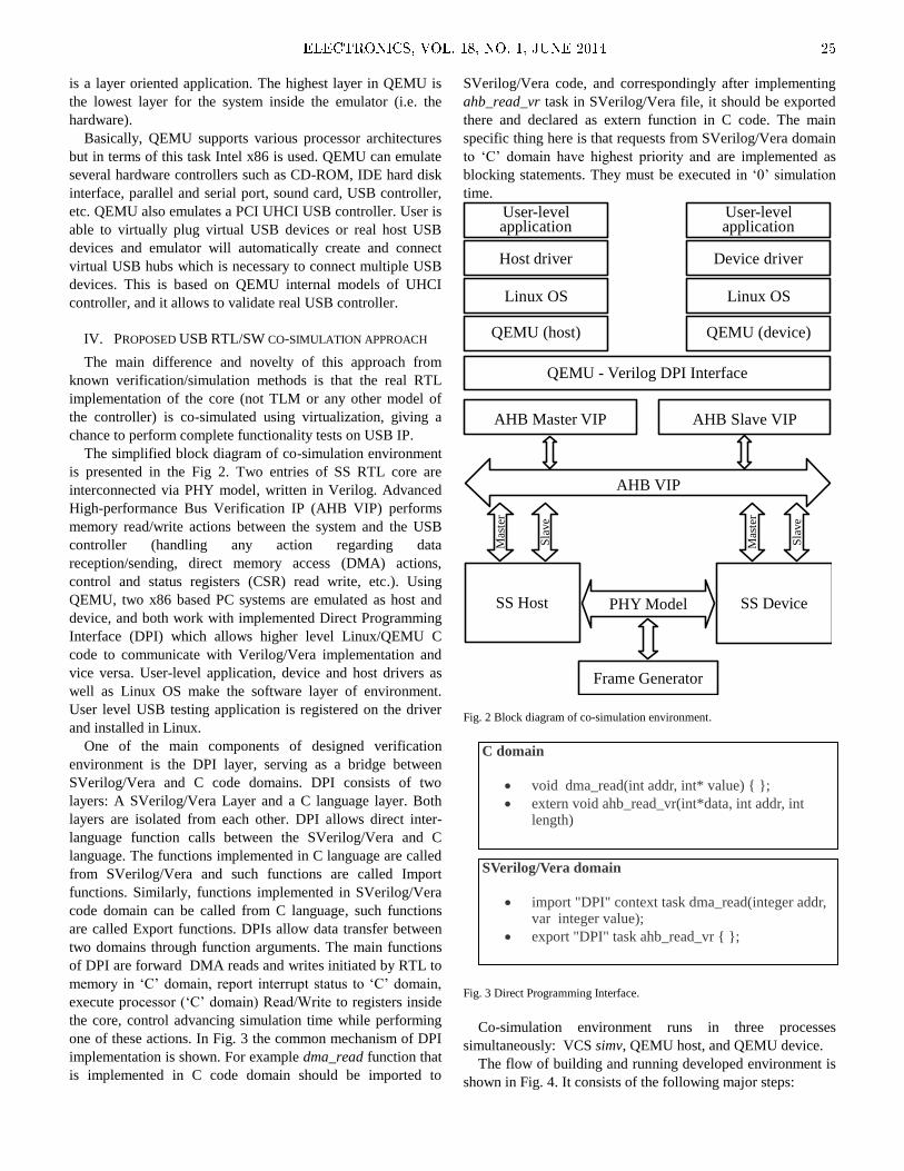
is a layer oriented application. The highest layer in QEMU is

the lowest layer for the system inside the emulator (i.e. the

hardware).

Basically, QEMU supports various processor architectures

but in terms of this task Intel x86 is used. QEMU can emulate

several hardware controllers such as CD-ROM, IDE hard disk

interface, parallel and serial port, sound card, USB controller,

etc. QEMU also emulates a PCI UHCI USB controller. User is

able to virtually plug virtual USB devices or real host USB

devices and emulator will automatically create and connect

virtual USB hubs which is necessary to connect multiple USB

devices. This is based on QEMU internal models of UHCI

controller, and it allows to validate real USB controller.

IV. PROPOSED USB RTL/SW CO-SIMULATION APPROACH

The main difference and novelty of this approach from

known verification/simulation methods is that the real RTL

implementation of the core (not TLM or any other model of

the controller) is co-simulated using virtualization, giving a

chance to perform complete functionality tests on USB IP.

The simplified block diagram of co-simulation environment

is presented in the Fig 2. Two entries of SS RTL core are

interconnected via PHY model, written in Verilog. Advanced

High-performance Bus Verification IP (AHB VIP) performs

memory read/write actions between the system and the USB

controller (handling any action regarding data

reception/sending, direct memory access (DMA) actions,

control and status registers (CSR) read write, etc.). Using

QEMU, two x86 based PC systems are emulated as host and

device, and both work with implemented Direct Programming

Interface (DPI) which allows higher level Linux/QEMU C

code to communicate with Verilog/Vera implementation and

vice versa. User-level application, device and host drivers as

well as Linux OS make the software layer of environment.

User level USB testing application is registered on the driver

and installed in Linux.

One of the main components of designed verification

environment is the DPI layer, serving as a bridge between

SVerilog/Vera and C code domains. DPI consists of two

layers: A SVerilog/Vera Layer and a C language layer. Both

layers are isolated from each other. DPI allows direct inter-

language function calls between the SVerilog/Vera and C

language. The functions implemented in C language are called

from SVerilog/Vera and such functions are called Import

functions. Similarly, functions implemented in SVerilog/Vera

code domain can be called from C language, such functions

are called Export functions. DPIs allow data transfer between

two domains through function arguments. The main functions

of DPI are forward DMA reads and writes initiated by RTL to

memory in ‘C’ domain, report interrupt status to ‘C’ domain,

execute processor (‘C’ domain) Read/Write to registers inside

the core, control advancing simulation time while performing

one of these actions. In Fig. 3 the common mechanism of DPI

implementation is shown. For example dma_read function that

is implemented in C code domain should be imported to

SVerilog/Vera code, and correspondingly after implementing

ahb_read_vr task in SVerilog/Vera file, it should be exported

there and declared as extern function in C code. The main

specific thing here is that requests from SVerilog/Vera domain

to ‘C’ domain have highest priority and are implemented as

blocking statements. They must be executed in ‘0’ simulation

time.

AHB Master VIP AHB Slave VIP

AHB VIP

QEMU - Verilog DPI Interface

QEMU (device)QEMU (host)

Linux OS Linux OS

Host driver Device driver

PHY Model

Frame Generator

SS Host SS Device

Sla

ve

Mas

ter

Sla

ve

Mas

ter

User-level application

User-level application

Fig. 2 Block diagram of co-simulation environment.

C domain

void dma_read(int addr, int* value) ;

extern void ahb_read_vr(int*data, int addr, int length)

SVerilog/Vera domain

import "DPI" context task dma_read(integer addr, var integer value);

export "DPI" task ahb_read_vr ;

Fig. 3 Direct Programming Interface.

Co-simulation environment runs in three processes

simultaneously: VCS simv, QEMU host, and QEMU device.

The flow of building and running developed environment is

shown in Fig. 4. It consists of the following major steps:

ELECTRONICS, VOL. 18, NO. 1, JUNE 2014 25

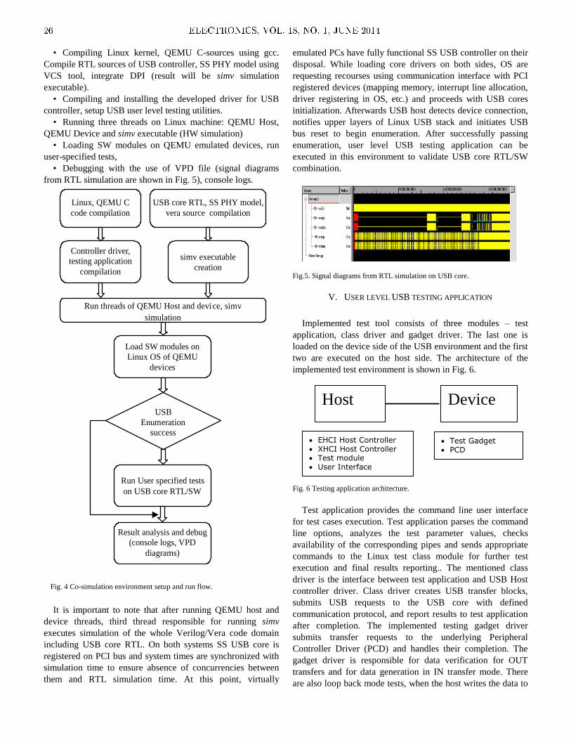
• Compiling Linux kernel, QEMU C-sources using gcc.

Compile RTL sources of USB controller, SS PHY model using

VCS tool, integrate DPI (result will be simv simulation

executable).

• Compiling and installing the developed driver for USB

controller, setup USB user level testing utilities.

• Running three threads on Linux machine: QEMU Host,

QEMU Device and simv executable (HW simulation)

• Loading SW modules on QEMU emulated devices, run

user-specified tests,

• Debugging with the use of VPD file (signal diagrams

from RTL simulation are shown in Fig. 5), console logs.

It is important to note that after running QEMU host and

device threads, third thread responsible for running simv

executes simulation of the whole Verilog/Vera code domain

including USB core RTL. On both systems SS USB core is

registered on PCI bus and system times are synchronized with

simulation time to ensure absence of concurrencies between

them and RTL simulation time. At this point, virtually

emulated PCs have fully functional SS USB controller on their

disposal. While loading core drivers on both sides, OS are

requesting recourses using communication interface with PCI

registered devices (mapping memory, interrupt line allocation,

driver registering in OS, etc.) and proceeds with USB cores

initialization. Afterwards USB host detects device connection,

notifies upper layers of Linux USB stack and initiates USB

bus reset to begin enumeration. After successfully passing

enumeration, user level USB testing application can be

executed in this environment to validate USB core RTL/SW

combination.

Fig.5. Signal diagrams from RTL simulation on USB core.

V. USER LEVEL USB TESTING APPLICATION

Implemented test tool consists of three modules – test

application, class driver and gadget driver. The last one is

loaded on the device side of the USB environment and the first

two are executed on the host side. The architecture of the

implemented test environment is shown in Fig. 6.

Fig. 6 Testing application architecture.

Test application provides the command line user interface

for test cases execution. Test application parses the command

line options, analyzes the test parameter values, checks

availability of the corresponding pipes and sends appropriate

commands to the Linux test class module for further test

execution and final results reporting.. The mentioned class

driver is the interface between test application and USB Host

controller driver. Class driver creates USB transfer blocks,

submits USB requests to the USB core with defined

communication protocol, and report results to test application

after completion. The implemented testing gadget driver

submits transfer requests to the underlying Peripheral

Controller Driver (PCD) and handles their completion. The

gadget driver is responsible for data verification for OUT

transfers and for data generation in IN transfer mode. There

are also loop back mode tests, when the host writes the data to

Fig. 4 Co-simulation environment setup and run flow.

Linux, QEMU C

code compilation

Controller driver,

testing application

compilation

USB core RTL, SS PHY model,

vera source compilation

simv executable

creation

Run threads of QEMU Host and device, simv

simulation

Load SW modules on

Linux OS of QEMU

devices

USB

Enumeration

success

Run User specified tests

on USB core RTL/SW

Result analysis and debug

(console logs, VPD

diagrams)

Host Device

EHCI Host Controller XHCI Host Controller Test module User Interface

Test Gadget PCD

26 ELECTRONICS, VOL. 18, NO. 1, JUNE 2014

the device first, then reads it back and verifies its accuracy.

For communication between host and device, vendor

specific protocol is developed (Table 1) in addition to standard

USB requests.

User interface module is a command line interface. Each

test case (or group of test cases) needs to be configured

individually with flexible input arguments through user

interface module. Each configuration parameters can be

divided into the following groups: endpoints parameters which

represent endpoint descriptors main fields and endpoint’s pair

number (interface, number, direction, type, and max packet

size), test parameters (mode, transfer size and iteration count).

A special algorithm is developed to handle errors. The

transfer buffers are filled with data using implemented

algorithm. This algorithm is common for the test gadget and

the host test module. Depending on the direction of the test,

the test module or test gadget will fill the transfer buffer. The

other part will verify the received data.

The USB test gadget provides functionality for

implementing the Communication protocol. The test gadget

handles all vendor specific requests, controlling endpoints and

interface.

VI. STATISTICS AND TEST RESULTS

Co-simulation environment requires significant resources

from host Linux machine. The analysis shows that major CPU

load is caused by simv executable running. Simulation

profiling shows that about 50% of CPU utilization by simv is

due to Verilog modules (core RTL design itself). The basic

timing statistics of co-simulation and CPU utilization are

follows:

• Compilation done – time 7.2 min (performing once

during setup)

• QEMU Host and Device booting – 2.5 min

• Driver loading done – time 1.3 min

• Core Initialization by driver done – time 1.2 min

• Simulating 1mSec – time 3.6 sec

• CPU Utilization Profile [%]: total time 20 min

Direct Programming Interface (DPI) 1.53%

Programming language interface (PLI) 24.45%

VCS for writing VCD and VPD files 6.82%

VCS for internal operations (KERNEL) 15.86%

Verilog Modules 50.69%

A SystemVerilog testbench program block 0.38%

Garbage Collector(PROGRAM GC) 0.27%

As it is shown in statistics analysis, it takes about 3–4s of

real time to simulate 1 ms of hardware work. Hence basic file

copy test between host and device systems via USB, with data

size, for example, 1MB takes about 3 minutes of real-time, but

based on simulation time copy is performed with 46-60MB/s

speed.

After driver loading phase and USB cores’ initialization by

SW on emulated host and device systems, various tests are

performed using the suggested test utility – control, bulk,

isochronous and interrupt traffic generation in both IN and

OUT directions. Also, test parameters like maximum packet

size, interval for periodic endpoints, burst for USB 3.0

transfers, stream count, etc. were modified during tests.

Obtained results are captured in Table 2.

VII. CONCLUSIONS

In this paper a new approach to USB controller RTL and

driver co-simulation and verification method is proposed. The

suggested method is based on virtualization techniques

(QEMU emulator) using USB SS core. The method is based

on the idea of using a real USB controller RTL model, instead

of TLM or other abstract models. The designed environment

allows identifying/debugging USB HW design easily,

debugging device driver before real tests on FPGA or SoC,

TABLE 2. LINUX USBTEST UTILITY TEST RESULTS IN CO-SIMULATION

ENVIRONMENT

Tes

t

Des

crip

tio

n

Max

pac

ket

size

Max

bu

rst

size

Tr.

siz

e

Inte

rval

Du

rati

on

Res

ult

Bulk in 1024 0 0.1M - 0.328s Pass

Bulk in 1024 10 0.1M - 0.18s Pass

Bulk out 1024 0 0.1M - 0.331s Pass

Bulk out 1024 10 0.1M - 0.19s Pass

Control in 512 - 1M - 2.083s Pass

Control out 512 - 1M - 2.063s Pass

Isochronous

in

1024 0 10M 1 1.5s Pass

Isochronous

out

1024 0 16K 14 19.09s Pass

Request Mnemonic Description/Purpose

DEV_CAP The device will return the

device capabilities.

CONF_EP_IF

Allows the host to change the

parameters of endpoints and

configure an interface.

TEST_SETUP The host sets the test

parameters.

TEST_STAT The device will return the Test

Case status.

CONTROL_WRITE Writes data to the control

pipe.

CONTROL_READ Reads data from the control

pipe.

SET_TR Provides to device for setting

up a transfer for an Endpoint.

RET_RES

The device will return the

results of the most recent

transfer.

DEV_RESET Resets the Device or Interface

to a known state.

TABLE 1 VENDOR SPECIFIC PROTOCOLS

ELECTRONICS, VOL. 18, NO. 1, JUNE 2014 27

reproducing and debugging issues emerging in the real

circumstances using signal diagrams obtained from simulation,

beginning device driver development and testing when

hardware is not available yet. A user level USB testing

application is also developed, which allows running custom

tests with various test parameters using different speeds. The

implemented application has the ability to ensure four types of

transfer running in virtual environment. The method is flexible

and does not depend on the USB controller or any other USB

IP’s RTL, and can be easily integrated into the environment

after minor changes in the USB PHY model.

REFERENCES

[1] Universal Serial Bus 3.0 Specification. Rev 1.0. - June 2011,

www.usb.org

[2] De Maria, E.A.A., Gho, E., Maidana, C.E., Szklanny, F.I., Tantignone,

H.R., A Low Cost FPGA based USB Device Core // IEEE 4th Southern

Conference on Programmable Logic, 2008, pp. 149-154.

[3] Babulu, K., Rajan, K.S., FPGA Implementation of USB Transceiver

Macrocell Interface with USB2.0 Specifications // ICETET '08. First

International Conference on Emerging Trends in Engineering and

Technology, July 2008, pp. 966-970.

[4] IEEE Computer Society, IEEE Standard System C Language Reference

Manual, 2005, pp. 423.

[5] OSCI, Transaction Level Modeling(TLM) Library, Release 1.0, 2005

[6] Anderson, R.B., Borowczak, M., Wilsey, P.A., The Use of Device

Simulation in Development of USB Storage Devices // IEEE 41st

Annual symposium, 2008, pp. 220-226.

[7] Xiaoping, B.; Shenlei, The Study on System Verification of USB2.0

Interface Protocol Control Chip Hardware Design // ICEE '07.

International Conference on Electrical Engineering, 2007, pp. 1-5.

[8] Puhar, P., Zemva, A., Functional Verification of a USB Host Controller

// IEEE 11th EUROMICRO Conference on Digital System Design

Architectures, Methods and Tools, 2008, pp. 735-740.

[9] Soba ski, I.; Sakowski, W., Hardware/software co-design in USB 3.0

mass storage application // IEEE International Conference on Signals

and Electronic Systems (ICSES), 2010, pp. 343-346..

[10] USB Testing on Linux, March 2007, http://www.linux-usb.org/usbtest/.

[11] SuperSpeed USB Compliance Testing

http://www.usb.org/developers/ssusb/testing

[12] QEMU open source processor emulator, http://www.qemu.org, 2013.

[13] Ribi re, A., Emulation of obsolete hardware in open source

virtualization software // IEEE 8th IEEE International Conference on

Industrial Informatics (INDIN), 2010, pp. 354-360.

28 ELECTRONICS, VOL. 18, NO. 1, JUNE 2014

Abstract—Vector network analyzer (VNA) is versatile

measuring equipment which is primarily used for two-port device

S parameters measurements. This paper addresses measurement

of capacitor parameters using VNA in broad frequency range.

The main attention is focused on the measurement accuracy of

capacitors parameters using VNA and proper de-embedding of an

experimental setup parasitics to get accurate results. Comparative

measurement error analysis for different measurement techniques

is presented. Suitability of each measurement technique for

measurements of capacitor parameters using VNA is discussed

and effect of the experimental setup parasitics on the

measurement results is addressed. Moreover useful procedures

for proper capacitor impedance measurement using VNA are

developed.

Index Terms—Capacitors, vector network analyzers,

measurements, measurement accuracy.

Original Research Paper

DOI: 10.7251/ELS1418029S

I. INTRODUCTION

APACITORS are used in many electronic devices, especially

in radio-frequency equipment, such as transmitters,

receivers, conducted electromagnetic interference filters, etc.

Capacitors capacitance is typically ranging from several pF

to several thousands of µF. The main parameters of a capacitor

are its capacitance C and impedance magnitude |Zc| (as a

function of frequency). Real capacitors, of course, have

parasitic parameters such as series resistance Rs (mainly lead

wires resistance), parallel resistance Rp (due to losses in

capacitor dielectric), equivalent series inductance (ESL) and

self-resonance frequency fres. Real capacitors can be

substituted by their equivalent circuit model shown in Fig.1

(a). However in practice when designing electronic circuits

with capacitors, more simple capacitor equivalent circuit

model is usually used as shown in Fig.1(b). In this model ESR

accounts for both Rp and Rs [1]. Usually knowing ESR is much

more important than Rp and Rs separately [2]. That is why

Manuscript received 15 April 2014. Received in revised form 7 June 2014.

Accepted for publication 11 June 2014.

This work was supported by the Project "Competence Centre of Latvian

Electric and Optical Equipment Production" co financed by the European

Union (agreement no. L-KC-11-0006). D. Stepins, G. Asmanis and A.

Asmanis are with the Latvian Electronic Equipment Testing Center, Riga,

Latvia (phone: +37128327653; e-mail: stepin2@inbox.lv).

capacitor manufacturers only give ESR values in their catalogs.

At a self-resonance frequency fres a capacitor has its

minimum |Zc|, which is equal to ESR (at fres). For f<fres, |Zc| is

decreasing function of f, but for f>fres, |Zc| increases as f

increases, Fig.2.

Accurate measurement of capacitor parameters (including

parasitic ones) is of major importance when designing

electronic equipment. For capacitor and inductor parameters

measurements in broad frequency range usually impedance

analyzers are used [3] – [10]. However the impedance

analyzers are expensive and the measurement frequency range

is usually limited up to several hundreds of MHz [3], [6], [10].

In contrast to the impedance analyzers, vector network

analyzers (VNA) are less expensive, more versatile and can be

used for capacitor parameters measurements in much broader

frequency range up to tens of GHz.

Measuring Capacitor Parameters Using Vector

Network Analyzers

Deniss Stepins, Gundars Asmanis, and Aivis Asmanis

C

ESLCESR

Parasitic parameters

ESLC Rs

Rp (a)

(b)

Fig. 1. Real capacitor equivalent circuit model (a) and its simplified

version (b).

Impe

dan

ce m

agnitude

Frequencyfres

ESR @ fres

Capacitive

reactance is

dominant

Inductive

reactance is

dominant

Fig. 2. Real capacitor impedance magnitude versus frequency.

ELECTRONICS, VOL. 18, NO. 1, JUNE 2014 29

For two-terminal passive electronic components

measurements using VNA, three measurement techniques can

be used: reflection (based on reflection coefficient S11

measurement), shunt-through (based on transmission

coefficient S21 measurements) and series-through techniques

(based on S21 measurements) as shown in Fig.3 [3], [6]. Shunt-

through technique is usually used for low-impedance passive

electronic components, while series-through technique for

high-impedance components [3].

Although different measurement techniques of two-terminal

passive electronic components are investigated in [3], [6] -

[10], no one of the papers consider measurement accuracy of

VNA techniques. Moreover suitability of each VNA technique

for capacitors parameters measurements is not addressed and

proper de-embedding of experimental setup parasitic

parameters is not considered in the papers. For example, in

[10] the main attention is focused on auto-balancing bridge

techniques for ESR measurements and VNA techniques are not

investigated thoroughly, in [6] inductors and capacitors

impedance measurement repeatability and temperature

dependence for the radio-frequency impedance analyzers and

VNA is comparatively investigated, but in [3] experimental

measurements of low-impedance inductors and ferrite complex

magnetic permeability using VNA are presented without

addressing any measurement accuracy issues.

The main original contribution of this paper is focused on

the measurement accuracy of capacitors parameters using

VNA and proper de-embedding of an experimental setup

parasitics to get accurate measurement results. Comparative

measurement error analysis for all the three techniques will be

presented. Suitability of each measurement technique for

capacitors parameters measurements using VNA will be

discussed and effect of the experimental setup parasitics on

capacitor measurement results will be addressed. Moreover

useful procedures for proper capacitor impedance

measurement using VNA will be developed.

II. MEASUREMENT OF CAPACITOR PARAMETERS

A. Experimental setups

In order to get capacitor impedance and other capacitor

parameters, S parameters should be measured first. When using

the reflection technique S11 should only be measured; for the

shunt-through technique S21 should only be measured; when

using the series-through technique S21 should only be measured

[3],[6]. For S parameters measurements VNA Rohde and

Schwarz ZVRE is used. Necessary capacitor parameters are

then extracted from the S parameters measured. The

measurements are done in the frequency range 100 kHz – 500

MHz, with VNA intermediate frequency filter bandwidth of

300 Hz and 1600 points per sweep. After the warm-up time of

one hour, full two-port TOSM (through-open-short-matched)

calibration has been performed to significantly reduce

systematic errors due to imperfect VNA cables and connectors.

Experimental setups used for the capacitor parameters

measurements are shown in Fig.4 – Fig.6. To perform one-port

reflection measurements, a capacitor is attached to one VNA

cable using type N RF connector (Fig.4(a)). To perform two-

port shunt-through capacitor measurement, two VNA cables

and capacitor are connected in parallel as shown in Fig.5(a).

To perform two-port series-through capacitor measurement,

two VNA cables and capacitor are connected in series as

VNA

Capacito

r

port 1 port 2VNA

Capacitor

port 1 port 2

(a) (b)

VNA

Capacitor

port 1 port 2

(c)

Fig. 3. Two terminal passive components measueremnt techniques using

VNA: (a) reflection technique; (b) shunt-through technique; (c) series

through technique.

VNA cable

calibrated

connectoruncalibrated

type N

connector

capacitor

under test

shorted

connector

CpRp

Ls Rs

VN

A P

ort 1

Uncalibrated

connector

Capacitor

under test

Vs

50

VNA

Z11s

Y11p

(a)

(b)

(c)

Fig. 4. (a) Experimental setup to perform the reflection technique; (b)

shorted N type connector; (c) equivalent circuit model.

30 ELECTRONICS, VOL. 18, NO. 1, JUNE 2014

VNA cables

Cp1Rp1

Ls1 Rs1

Uncalibrated

Connector 1Capacitor

under test

VN

A p

ort 1

VN

A p

ort 2

Vs

50

VNA

50

VNA

VVCp2 Rp2

Ls2Rs2

Y11p1 Y11p2

Z11s1 Z11s2Zc

Uncalibrated

Connector 2

(a)

(b)

Fig. 5. Experimental setup to perform the shunt-through technique (a) and its equivalent circuit model (b).

shown in Fig.6(a).

Since it is impossible to make TOSM calibration for the N

type RF connectors to which the capacitors are attached in the

experiments, the parasitic parameters (parasitic equivalent

series impedance Z11s and parasitic equivalent conductance

Y11p) of the connectors should be taken into account and

removed from the capacitors measurement results

mathematically using de-embedding.

B. De-embedding of the connectors parasitics

To de-embed the connector’s parasitics, simple equivalent

circuit models of the experimental setups for all the three

measurement techniques are developed in the paper as shown

in Fig.4 – Fig.6. The equivalent circuit models can give us a

possibility to derive expressions for capacitors complex

impedance Zc calculations.

For the reflection technique it can be derived

s

p

ZY

11

1111

c1/Z

1Z

, (1)

where Z11 is complex impedance which can be calculated from

the measured reflection coefficient S11 as follows [3]

2

1111

11

2

11

11

1111

cos21

sin2150

S-1

S150Z

SS

SjS

. (2)

If parasitics of the connectors are not high, then approximately

Zc can be calculated using (2).

For the shunt-through technique it can be derived

))(( 21121121111121

211211211111111

50150100100

15050250050

psspb

psssasc

YZZYZS

)Y(ZZZZZZ

, (3)

where )()( 211111111211211 505011 spppsa ZYYYZZ

)()( 211111211211 2500501 pppsb YYYZZ

Z11s1 and Z11s2 are parasitic equivalent series impedances of

the 1st and the 2

nd uncalibrated connectors respectively; Y11p1

and Y11p2 are parasitic equivalent conductances of the 1st and

the 2nd

uncalibrated connectors respectively.

If parasitics of the connectors are not high, then

approximately Zc can be calculated as follows [3]

2

2121

21

2

2121

21

21c

cos21

sincos25

S-1

S52Z

SS

SjSS

. (4)

For the series-through technique it can be derived

s

p

sps

ZY

ZYZZZ

11

111

11111

21

1

c501

5050S

2Z

Z

, (5)

ELECTRONICS, VOL. 18, NO. 1, JUNE 2014 31

VNA cables

Cp1Rp1

Ls1 Rs1

Uncalibrated

Connector 1Capacitor

under test

VN

A p

ort 1

VN

A p

ort 2

Vs

50

VNA

50

VNA

VVCp2 Rp2

Ls2Rs2

Y11p1 Y11p2

Z11s1 Z11s2Zc

Uncalibrated

Connector 2

(a)

(b)

Fig. 6. Experimental setup to perform the series-through technique (a) and its equivalent circuit model (b).

where Zs=Z11s1+Z11s2; Z1=1/(1/50+Y11p2).

If parasitics of the connectors are not high, then

approximately Zc can be calculated as follows

212121

21c

sin1

cos100

S

S-1100Z

Sj

S

(6)

C. Determination of the connectors parasitics

Typical RF N type connector parasitic capacitance is about 1

pF and inductance of shorted connector is about 10nH. This

means that parasitic resonant frequency of the connectors is

well above 1 GHz. Since all the measurements are done in the

frequency range up to 500 MHz, then parasitic series

impedances Z11s1 and Z11s2 can be determined by measuring

impedance of shorted connectors, but parasitic parallel

conductances Y11p1 and Y11p2 can be determined by measuring

conductance of open connectors. The measurement results for

the two connectors used in the experiments are shown in Fig.7.

As it can be seen the shorted connector impedance magnitude

increases almost linearly as frequency increases, because

inductive reactance (due to Ls) is dominant, and conductance

magnitude of the open connectors also increases almost

linearly because capacitive conductance (due to Cp) dominates.

D. Procedures for capacitor impedance measurement

In this section the procedures developed for capacitor

impedance measurements using all the three measurement

105

106

107

108

10-3

10-2

10-1

100

101

102

frequency, Hz

im

pe

da

nce

mag

nitu

de,

oh

ms,

connector 1

connector 2

105

106

107

108

109

10-6

10-5

10-4

10-3

10-2

frequency, Hz

con

du

cta

nce

ma

gnit

ud

e,

S

(a) (b)

Fig. 7. Measured impedance magnitude of short connectors (a) and conductance magnitude of open connectors (b).

32 ELECTRONICS, VOL. 18, NO. 1, JUNE 2014

techniques are presented.

Procedure for the capacitor impedance measurement using

the reflection technique

make full two-port TOSM calibration;

connect the type N RF connector with soldered

capacitor (Fig.4(a)) to VNA cable;

measure complex S11;

desolder the capacitor from the connector and

connect shorted connector without capacitor

(Fig.4(b)) to the VNA cable and measure complex

Z11s;

connect open connector without capacitor to the

VNA cable and measure complex Y11s;

calculate complex impedance Z11 using (2);

de-embed the connector parasitics using (1) to

calculate the capacitor complex impedance Zc;

end.

Procedure for the capacitor impedance measurement using

the shunt-through technique

make full two-port TOSM calibration;

connect both N type RF connectors in parallel and

solder a capacitor under test to them (Fig.5(a));

measure complex S21 using VNA;

measure both connectors parasitcs Z11s1, Z11s2, Y11p1

and Y11p2;

calculate the capacitor complex impedance Zc using (3);

end.

Procedure for the capacitor impedance measurement using

the series-through technique

make full two-port TOSM calibration;

solder a capacitor under test to both connectors in

series as shown in Fig.6(a);

connect them to VNA cables;

measure complex S21 (with the capacitor under test);

measure both connectors parasitics Z11s1, Z11s2, Y11p1

and Y11p2;

calculate the capacitor complex impedance Zc using

(5);

end.

E. Extraction of capacitor parameters from complex

impedance Zc

capacitance C can be calculated at the lowest

frequency f1 (at which parasitic inductive reactance

is negligible):

||2

1C

1 cZimagf (7)

capacitor ESR(f)=realZc(f);

capacitor resonant frequency fres is frequency at

which capacitor complex impedance magnitude |Zc|

is minimum;

capacitor equivalent series inductance can be

calculated as follows:

Cf

ESLres

224

1

. (8)

F. Comparison of the measurement results

Using the procedures developed capacitors with different

105

106

107

108

10-1

100

101

102

103

Frequency, Hz|Z

c|, o

hm

s

1 2 3 4 5 6 7 8

x 105

200

400

600

800

1000

1200

1400

1600

Frequency, Hz 4 6 8 10 12 14 16

x 107

10-1

100

Frequency, Hz

A

B

CD

Shunt-through

Series-

through

Reflection

|Zc|, o

hm

s

(a)

105

106

107

108

0

50

100

150

200

250

300

frequency, Hz

ES

R,

oh

ms

1.5 2 2.5 3 3.5

x 105

-6

-4

-2

0

2

4

6

8

frequency, Hz

ES

R,

oh

ms

Frequency, Hz

A

4 6 8 10 12

x 107

0.1

0.2

0.3

0.4

0.5

ES

R,

oh

ms

Frequency, Hz

ES

R,

oh

ms

ES

R,

oh

ms

Frequency, Hz

Frequency, Hz Frequency, Hz

Shunt-through

Reflection

Series-

through

Series-

through

Reflection

(b)

Fig. 8. Measured 1nF capacitor impedance magnitude (a) and ESR (b) versus

frequency.

ELECTRONICS, VOL. 18, NO. 1, JUNE 2014 33

nominal capacitance values (1nF, 10nF, 100nF and 1000nF)

have been measured using the reflection, shunt-through and

series-through techniques. The capacitors with nominal

capacitances of 1nF, 100nF and 1000nF are metalized

polypropylene film capacitors with capacitance tolerance of

±5%, but the capacitor with nominal capacitance of 10nF is

polyester film capacitor with tolerance of ±20%.

Measured |Zc| and ESR versus frequency for several

capacitors are comparatively depicted in Fig.8 and Fig.9. But

in Table 1 measured capacitor C and ESR (at f=100kHz) using

VNA and high-precision LCR meter Instek LCR 819 are

tabulated. Analysis of the measurement results and

measurement errors will be presented in section IV.

TABLE 1

COMPARISON OF MEASURED CAPACITANCE AND ESR (AT 100KHZ) USING

HIGH-PRECISION LCR METER AND VNA FOR DIFFERENT CAPACITORS

Nominal capacitance, nF 1 10 100 1000

LCR meter C, nF 1 8.48 100.2 998.7

ESR, Ω 2.5 3.6 0.29 0.04

VNA

refle-

ction

C, nF 0.96 8.22 98.5 984.8

ESR, Ω -2.61 2.86 0.19 0.041

shunt-

through

C, nF 1.25 8.74 99.3 991

ESR, Ω 288 7.8 0.28 0.04

series-

through

C, nF 0.98 8.29 99 1200

ESR, Ω -5.9 2.86 0.59 0.39

G. Effect of connectors parasitics on capacitor parameters

measurements

It is interesting to observe how uncalibrated connectors

parasitics affect measurement results. Measured |Zc| and ESR

versus frequency before (using (2), (4) and (6)) and after

(using (1), (3) and (5)) de-embedding is depicted in Fig.10. As

it can be seen the reflection and the series-through techniques

are very sensitive to the connectors parasitics in MHz range for

both ESR and |Zc| (Fig.10(a,b,e,f)). If the connector parasitics

are not removed from the measurement results using (1) and

(5), then measured fres is noticeably lower, but |Zc| is noticeably

higher (for f above fres) than it is. This is mainly due to

parasitic inductance of the connectors used.

|Zc| and fres measured using the shunt-through technique is

much less affected due to the connector parasitics. For f up to

several hundreds of MHz effect of the connector’s parasitics is

negligible (Fig.10(c)). However ESR measured using the

shunt-through technique is affected much higher due to

connectors parasitics for f higher than several tens of MHz

(Fig.10(d)).

III. CALCULATION OF THE CAPACITOR PARAMETERS

MEASUREMENT ERRORS

Since capacitor Zc, ESR and other parameters are indirect

measurement results then for measurement error calculation

partial differentiation method [12] can be used. When partial

errors are known, indirect measurement absolute error (∆Y)

can be calculated

K

i

i

i

xx

YY

1

2

, (9)

and relative error

% ,Y

Y 100 , (10)

where ixY / is partial derivative with respect to argument xi;

∆xi is xi argument absolute error.

For the reflection technique capacitor impedance is the

function of 6 arguments (according to (1) and (2)):

x1=|S11|, x2=φ; x3=|Z11s|, x4=φs, x5=|Y11p|, x4=φp,

where S11= |S11|ejφ

, Z11s=|Z11s|ejφs, Y11p==|Y11p|e

jφp.

For the shunt-through technique capacitor impedance is

the function of 10 arguments (according to (3)):

x1=|S21|, x2=φ; x3=|Z11s1|, x4=φs1, x5=|Y11p1|, x6=φp1,

x7=|Z11s2|, x8=φs2, x9=|Y11p2|, x10=φp2.

For the series-through technique capacitor impedance

is the function of 10 arguments (according to (5)):

x1=|S21|, x2=φ; x3=|Z11s1|, x4=φs1, x5=|Y11p1|, x6=φp1,

x7=|Z11s2|, x8=φs2, x9=|Y11p2|, x10=φp2.

Absolute measurement errors of the main capacitor

parameters can be calculated using the following expressions:

K

i

i

i

cc x

x

ZZESR

1

2

ReRe (11)

|Zc|, o

hm

s

Frequency, Hz10

510

610

710

810

-2

10-1

100

101

102

Reflection

Series-through

Shunt-through

(a)

105

106

107

108

-1.5

-1

-0.5

0

0.5

1

Frequency, Hz

ES

R, o

hm

s

Shunt-through

Reflection

Series-through

(b)

Fig. 9. Measured 100nF capacitor impedance magnitude (a) and ESR (b)

versus frequency.

34 ELECTRONICS, VOL. 18, NO. 1, JUNE 2014

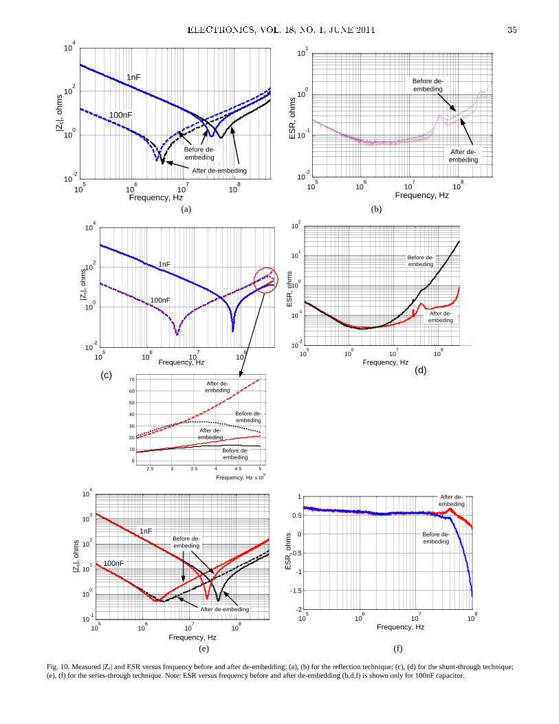
105

106

107

108

10-2

100

102

104

|Zc|, o

hm

s

Frequency, Hz

Before de-

embeding

After de-embeding

1nF

100nF

Frequency, Hz

ES

R,

oh

ms

105

106

107

108

10-2

10-1

100

101

Before de-

embeding

After de-

embeding

(a) (b)

2.5 3 3.5 4 4.5 5

x 108

0

10

20

30

40

50

60

70

105

106

107

108

10-2

100

102

104

Before de-

embeding

Frequency, Hz

|Zc|, o

hm

s

After de-

embeding

After de-

embeding

Before de-

embeding

1nF

100nF

105

106

107

108

10-2

10-1

100

101

102

Frequency, Hz

After de-

embeding

Before de-

embeding

ES

R,

oh

ms

Frequency, Hz

(c)(d)

105

106

107

108

10-1

100

101

102

103

104

Before de-

embeding

After de-embeding

|Zc|, o

hm

s

Frequency, Hz

105

106

107

108

-2

-1.5

-1

-0.5

0

0.5

1

ES

R,

ohm

s

Frequency, Hz

Before de-

embeding

After de-

embeding

1nF

100nF

(e) (f)

Fig. 10. Measured |Zc| and ESR versus frequency before and after de-embedding: (a), (b) for the reflection technique; (c), (d) for the shunt-through technique;

(e), (f) for the series-through technique. Note: ESR versus frequency before and after de-embedding (b,d,f) is shown only for 100nF capacitor.

ELECTRONICS, VOL. 18, NO. 1, JUNE 2014 35

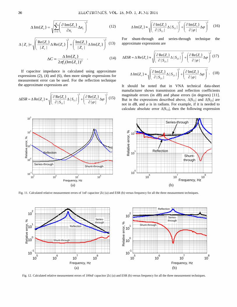
K

i

i

i

cc x

x

ZZ

1

2

ImIm (12)

22

Im||

ImRe

||

Re||

c

c

cc

c

cc Z

Z

ZZ

Z

ZZ (13)

2

1 )(Im2

Im

c

c

Zf

ZC

. (14)

If capacitor impedance is calculated using approximate

expressions (2), (4) and (6), then more simple expressions for

measurement error can be used. For the reflection technique

the approximate expressions are

22

11

11 ||

Re||

||

ReRe

cc

c

ZS

S

ZZESR (15)

22

11

11 ||

Im||

||

ImIm

cc

c

ZS

S

ZZ (16)

For shunt-through and series-through technique the

approximate expressions are

22

21

21 ||

Re||

||

ReRe

cc

c

ZS

S

ZZESR (17)

22

21

21 ||

Im||

||

ImIm

cc

c

ZS

S

ZZ . (18)

It should be noted that in VNA technical data-sheet

manufacturer shows transmission and reflection coefficients

magnitude errors (in dB) and phase errors (in degrees) [11].

But in the expressions described above, Δ|S11| and Δ|S21| are

not in dB, and φ is in radians. For example, if it is needed to

calculate absolute error Δ|S11|, then the following expression

105

106

107

108

10-1

100

101

102

103

Frequency, Hz

Re

lative e

rror,

%

Shunt-throughSeries-through

Reflection

106

107

108

100

101

102

Frequency, Hz

Rela

tive e

rror,

%

Shunt-

through

Series-through

Reflection

(a) (b)

Fig. 11. Calculated relative measurement errors of 1nF capacitor |Zc| (a) and ESR (b) versus frequency for all the three measurement techniques.

105

106

107

108

10-1

100

101

102

Frequency, Hz

Rela

tive e

rror,

%

Shunt-through

Series-

through

Reflection

105

106

107

108

10-1

100

101

102

Frequency, Hz

Rela

tive

err

or,

% Shunt-through

Reflection

Series-

through

(a) (b)

Fig. 12. Calculated relative measurement errors of 100nF capacitor |Zc| (a) and ESR (b) versus frequency for all the three measurement techniques.

36 ELECTRONICS, VOL. 18, NO. 1, JUNE 2014

should be used

)(||||/)||(

11020

111111

dBSSS , (19)

where dB

S ||11

is reflection coefficient measurement

uncertainty in dB from VNA data-sheet. In its turn, phase

absolute error (in radians) from VNA data-sheet can be

calculated as follows

180

deg , (20)

From VNA ZVRE data-sheet [11] it can be deduced that in

frequency range 20kHz – 4GHz: dB

S ||11

<0.4dB and Δφdeg<3o

(when |S11| is in range -15dB – +3dB); dB

S ||11

<1dB and

Δφdeg<6o (when |S11| is in range -25dB – -15dB). Accuracy of

transmission measurements: in the frequency range 20kHz –

300kHz: dB

S ||21

<0.2dB and Δφdeg<2o (when |S21| is in range -

20dB – +3dB); dB

S ||21

<0.5dB and Δφdeg<4o (when |S21| is in

range -20dB – -30dB); in the frequency range 300 kHz to 1

MHz: dB

S ||21

<0.1 dB or Δφdeg<1°; in the frequency range

1MHz to 4 GHz: dB

S ||21

<0.05 dB or Δφdeg<0.4°. This data

will be used for capacitors measurement error calculation.

Calculated relative measurement errors of ESR and |Zc| versus

frequency for all the three measurement techniques are shown

in Fig.11 and Fig.12. In the next section the measurement error

analysis will be presented.

IV. ANALYSIS OF THE MEASUREMENT RESULTS AND

MEASUREMENT ERRORS

Capacitors impedance magnitude |Zc| measurement analysis

Results presented in Fig.11 and Fig.12 clearly show that

measurement error of capacitors |Zc| depends not only on

capacitor impedance magnitude (and frequency) but also on

the measurement technique used.

For the shunt-through technique, the lower |Zc| is, the lower

measurement error is. The best measurement accuracy (below

1%) can be achieved at fres and in the vicinity of it using the

shunt-through technique. When using the technique for

|Zc|>30Ω, the measurement error exceeds several %. In kΩ

range the shunt-through technique exhibits very poor accuracy

(region A in Fig, 8(a)), because |S21| is very close to 0dB.

As opposed to the shunt-through technique, series-through

technique exhibits lower measurement error for higher |Zc|.

Measurement accuracy at fres and in the vicinity of it using the

series-through technique is very poor, because |S21| is very

close to 0dB. However when |Zc|>30Ω, the measurement error

is lower than several %, and in kΩ range the series-through

technique exhibits very good accuracy.

The reflection technique should not be used for capacitor

parameters measurements because it can give accurate results

only when capacitor |Zc| slightly differs from 50Ω (Fig.11(a)).

Capacitors resonant frequency fres measurement analysis

The best suited technique for capacitor fres measurement is

the shunt-through technique, because measurement accuracy of

capacitor impedance at fres and in the vicinity of it is very good

(Fig.11(a) and Fig.12(a)) and this technique is less sensitive to

the connectors parasitics.

Capacitors capacitance C measurement analysis

C measurement accuracy highly depends on the measurement

technique used. Since C is calculated using (7) and capacitor

|ImZc| at f1 can vary from hundreds of mΩ to kΩ (depends on

capacitor C), then for C measurements it is better to use the

shunt-through technique when C>50nF. However, when

C<50nF, then the series-through technique is the best choice

for C measurements. This can also be deduced from the Table

1. For capacitors with nominal capacitance values of 100nF

and 1000nF, the lowest difference between C values measured

using VNA and high-precision LCR meter is achieved using

the shunt-through technique (the difference below 1%).

However, for capacitors with nominal capacitance of 1nF and

10nF, the lowest difference between C values measured using

VNA and high-precision LCR meter is achieved using the

series-through technique (the difference below 3%). The

reflection technique should not be used for capacitance

measurements.

Capacitors ESR measurement analysis

According to the results presented in Table 1 and Fig.8(b) -

Fig.12(b) the most problematic parameter to measure

accurately with VNA is capacitor ESR. Only the shunt-through

technique should be used for accurate ESR measurements.

However there are some limitations. ESR can accurately be

measured only at fres and in vicinity of it (ESR measurement

error below 3% can be achieved). For frequencies which are

much higher or lower than fres the measurement accuracy can

be very poor, even using the shunt-through technique, because

when capacitor reactance is much higher than its ESR, then the

measurement error can increase enormously. Moreover

accurate measurements of ESR of capacitors with C lower than

several tens of nF are impossible: series-through and reflection

techniques for capacitors with C below 1nF, can give even

negative ESR which is completely unrealistic (Table 1). Even

the shunt-through technique gives very erroneous ESR

measurement results for small-capacitance capacitors. So ESR

measurements of small-capacitance capacitors (below 10nF)

using VNA is completely useless, because of very poor

measurement accuracy.

V. CONCLUSION

Vector network analyzers can be very useful for accurate

capacitor impedance, resonant frequency, capacitance and ESL

measurements in broad frequency range if proper measurement

technique and de-embedding is used. Measurement accuracy of

several % and even lower can be achieved using proper

measurement technique. Measurement error of capacitors

ELECTRONICS, VOL. 18, NO. 1, JUNE 2014 37

impedance and ESR depends not only on capacitor impedance

magnitude (and frequency) but also on the measurement

technique used.

The best suited technique for capacitor fres measurement is

the shunt-through technique, because measurement accuracy of

capacitor impedance at fres and in the vicinity of it is very good

(even below 1%) and this technique is less sensitive to the

experimental setup parasitics. For capacitor impedance

measurements in broad frequency range (when capacitor |Zc|

can change from mΩ to kΩ) it is better to use combination of

the shunt-through and series-through techniques: when |Zc| is

below several tens of ohms, then it is better to use shunt-

through technique; when |Zc| is above several tens of ohms,

then it is better to use series-through technique. The reflection

technique should not be used for capacitor parameters

measurements because, firstly, it can give accurate results only

when capacitor |Zc| slightly differs from 50Ω and secondly, it is

very sensitive to uncalibrated connectors parasitics.

The most problematic parameter to measure accurately with

VNA is capacitor ESR. Only shunt-through technique should

be used for accurate ESR measurements. However there are

some limitations. ESR can accurately be measured only at fres

and in vicinity of it (ESR measurement error below 3% can be

achieved). For frequencies which are much higher or lower

than fres the measurement accuracy can be very poor, even

using shunt-through technique, because when capacitor

reactance is much higher than its ESR, then the measurement

error can increase enormously. Accurate measurements of ESR

of capacitors with C lower than several tens of nF are

impossible. ESR measurements of small-capacitance

capacitors using VNA is completely useless.

Overall it can be concluded that VNA can substitute more-

expensive impedance analyzers for accurate capacitor

parameters measurements in broad frequency range with some

limitations in terms of ESR measurements.

REFERENCES

[1] Kazunari Okada, Toshimasa Sekino. Impedance Measurement

Handbook. Agilent Technologies, 2006.

[2] A.M.R. Amarel, A.J.M. Cordoso, “An economic offline technique for

estimating equivalent circuit of aluminum electrolytic capacitors,” IEEE

Transactions on Instrumentation and Measurement, vol.57, No.12, pp.

2697 – 2710, Dec. 2008.

[3] R. Dosoudil, „Determination of permeability from impedance

measurement using vector network analyzer,” Journal of electrical

engineering, vol. 63, No.7, pp. 97-101, Oct. 2012.

[4] Satish Prabhakaran, Charles Sullivan, "Impedance-analyzer

measurements of high-frequency power passives: Techniques for high

power and low impedance," In proc. IEEE Industry Applications

Conference, Pittsburgh, PA, USA, 2002, pp. 1360 – 1367.

[5] William B. Kuhn, Adam P. Boutz, "Measuring and reporting high

quality factors of inductors using vector network analyzers," IEEE

Transactions on Microwave Theory and Techniques, vol.58, No.4, pp.

1046-1055, Apr. 2010.

[6] Advanced Impedance Measurement Capability of the RF I-V Method

Compared to the Network Analysis Method. Agilent Application Note

No. 1369-2.

[7] Ultra Low Impedance Measurements Using 2-Port Measurements.

Agilent Application Note, 2004.

[8] L.D. Smith, D. Hockanson, “Distributed SPICE circuit model for

ceramic capacitors,” In. proc. Electronic Components and Technology

Conference, 2001, pp. 523-528.

[9] Rosa M. García Salvador, José A. Gázquez Parra, Nuria Novas

Castellano, “Characterization and Modeling of High-Value Inductors in

ELF Band Using a Vector Network Analyzer,” IEEE Transactions on

Instrumentation and Measurement, vol.62, No.4, pp. 415-423, Feb.

2013.

[10] Gregory L. Amorese, "Reducing ESR measurement errors," Microwaves

& RF, vol. 42, No.4, 2003.

[11] Vector Network Analyzer Family ZVR datasheet. Rohde and Schwarz.

[12] John R. Taylor, An Introduction To Error Analysis: The Study Of

Uncertainties In Physical Measurements. Sausalito, University Science

Books, 1996.

38 ELECTRONICS, VOL. 18, NO. 1, JUNE 2014

Abstract—A novel data-driven gradient descent (GD) adaptive

controller, for discrete-time single-input and single output (SISO)

systems, is presented. The controller operates as the least mean

squares (LMS) algorithm, applied to a nonlinear system with

feedback. Normalization of the learning rate parameter provides

robustness of the overall system to modeling errors and

environment nonstationarity. Convergence analysis reveals that

the controller forces tracking error to zero, with bounded control

signal and the controller weights. The experiments on the

benchmark systems support the analysis.

Index Terms—Data-Driven Controller, Gradient Descent

Algorithms, Direct Adaptive Control, Nonlinear SISO Systems,

Discrete Time.

Original Research Paper

DOI: 10.7251/ELS1418039K

I. INTRODUCTION

ONTROL means decision making. In order to decide well,

one has to have a goal, as well as, information on a

controlled process and process environment. Within automatic

control setup, the goal specifies desired behavior of the overall

system. Information, regarding the process and influence of the

environment, is given by the process model and/or process

measurements. In many automatic control applications process

model is not available. Instead, process measurements contain

information on the process behavior. Therefore, many control

algorithms were developed to cope with this situation. Usually,

they are referred to as data-driven or model-free. This

emphasizes situation where control is based, mainly, on the

available measurement data. In these situations, concepts like

feedback linearization [1], regardless their firm theoretical

foundation and good performance, are not applicable. If we

look back to the past, probably, the first data-driven control

Manuscript received 9 May 2014. Accepted for publication 11 June 2014.

I. R. Krcmar is with the Faculty of Electrical Engineering, University of

Banja Luka, Banja Luka, Bosnia and Herzegovina (phone: +387-65-927-212;

fax: +387-51-211-408; e-mail: ikrcmar@etfbl.net).

M. M. Bozic is with the Faculty of Electrical Engineering, University of

Banja Luka, Banja Luka, Bosnia and Herzegovina (e-mail:

mbozic@etfbl.net).

P. S. Maric is with the Faculty of Electrical Engineering, University of

Banja Luka, Banja Luka, Bosnia and Herzegovina (e-mail:

pmaric@etfbl.net).

procedure is one proposed by Ziegler and Nichols for tuning

proportional-integral-derivative (PID) controllers. However,

many data-driven control algorithms were reported in the

literature, till now. These are virtual reference feedback tuning

(VRFT), iterative feedback tuning (IFT) and data-driven

model-free adaptive control (MFAC), to mention a few. The

VRFT is reference model adaptive control technique. Within

VRFT framework, it is assumed that controller structure is

known a-priori and controller parameters are determined by

system identification procedure, using virtual reference signal.

It is designed for discrete-time single-input and single output

(SISO) linear time invariant (LTI) systems. The VRFT

procedure may produce controller that results in a non stable

closed loop system [2,3]. The IFT, also proposed for an

unknown discrete-time SISO LTI system, determines

controller parameters through iterative gradient-based local

search procedure. Computation of the gradient of criterion

function, with respect to the controller parameters, is based on

available input/output (I/O) measurement data of the

controlled plant [4]. The MFAC approach, in opposition to the

VRFT and IFT, was developed for a class of discrete-time

nonlinear systems. The main characteristic of the MFAC is

utilization of local dynamic linearization data models. The

models are computed along the dynamic operation points of

the closed-loop system. Computation is performed by the

dynamic linearization techniques, with a pseudo-partial

derivative concept, based on the real-time I/O measurements

of the controlled plant [3]. The above mentioned algorithms,

i.e. VRFT, IFT and data-driven MFAC, are direct adaptive

control algorithms, as they tune controller without prior plant

identification procedure. Further, in applications rich with

measurement data, regarding processes with high complexity,

neural networks (NNs), with their ability to approximate

functions through training procedure [5, 1], might be a good

solution. Specially, in nonlinear control tasks, NNs are

employed as nonlinear process models and/or nonlinear

controllers [6, 7, 1]. However, design of an appropriate NN,

meaning choice of an NN structure, input and output vectors,

training set and training algorithm, might be a difficult task.

Within signal prediction applications, we design a model that

should produce, on its output, the desired signal. Usually, the

model is parameterized and model parameters are tuned in the

real-time based on the incoming process measurements, i.e.

Data-Driven Gradient Descent Direct Adaptive

Control for Discrete-Time Nonlinear SISO

Systems

Igor R. Krcmar, Milorad M. Bozic, and Petar S. Maric

C

ELECTRONICS, VOL. 18, NO. 1, JUNE 2014 39

adaptively, in order to minimize a certain criterion. The

criterion is a function of the error signal, the signal that

represents the difference between some desired signal and the

model output [8]. Similar setup one can find in the automatic

control reference tracking tasks. In the reference tracking

tasks, the controller is tuned, so the overall system output

tracks the reference signal, as close as possible. Thus, adaptive

signal prediction and reference tracking control are similar

problems, as they can share the same criterion to be minimized

through the parameters correction procedure. For the given

parameterization of the process model, different procedures

can be applied to achieve optimal value of the model

parameters, regarding the imposed criterion. The gradient

descent (GD) approach performs search for the optimal value

of the parameters, in the parameter space, as it corrects the

parameter values in direction opposite to the gradient of the

criterion. A common choice for the criterion is a function of

the squared error. Models, applied in the signal prediction

tasks, with the feedback from the output to the input, introduce

nonlinearity into the signal prediction algorithm. Algorithms,

based on such models, are referred to as recurrent [8]. The

least mean squares (LMS) algorithm, as a member of the GD

class, is a simple, yet most frequently used algorithm for signal

prediction and system identification. However, it might have a

poor performance, when applied to a nonlinear signal and in

varying environment [10]. To that cause, a class of normalized

algorithms has been developed [12, 8, 9, 10]. They

successfully cope with process nonlinearity and

nonstationarity, thus provides faster convergence and higher

accuracy. The proposed data-driven GD adaptive controller

relies on the ideas established within signal prediction

framework. It is direct adaptive controller, designed for

discrete-time SISO nonlinear system to perform reference

tracking. The controller is parameterized, thus provides linear

combination of the reference signal and the output signal

discrete-time samples. The parameters are tuned, in the real-

time, through the GD procedure, to minimize a certain

criterion. The criterion is square of the instantaneous output

error, therefore the algorithm operates as the LMS algorithm

applied to a nonlinear system with feedback. In order to cope

with modeling errors and environment nonstationarity, the

learning rate is modified as in normalized algorithms [9, 10,

12]. The proposed algorithm has ability of a constant

disturbance rejection. Convergence analysis of the proposed

algorithm can be performed, following the approach given in

[11, 10]. The rest of the paper is organized as follows. In the

Section 2, problem formulation and the controller design

procedure are given. The Section 3 gives convergence

analysis, as well as, analysis of the disturbance rejection ability

of the proposed algorithm. The Section 4 contains

experimental verification of the algorithm, while the Section 5

concludes the paper.

II. PROBLEM FORMULATION AND CONTROLLER DESIGN

PROCEDURE

It is assumed that the controlled plant is discrete-time

nonlinear SISO system, described by the equation

( 1) ( ( ), ( 1), , ( );

( ), ( 1), , ( )) ( ),

y

u

y k f y k y k y k n

u k u k u k n f k

(1)

where ( )y k R and ( )u k R are the system output and

input, respectively, yn and

un are the unknown orders, and

k denotes discrete-time instant. Further, ( )f R is some

nonlinear function with continuous partial derivatives with

respect to its arguments. The controller parameterization is

given by the equation

1 2

1

2 2

( ) ( ) ( ) ( ) ( 1)

( ) ( 1) ( ) ( )

( ) ( 1) ( ) ( 1),

c c

c c

n c n

n n c

u k w k r k w k r k

w k r k n w k y k

w k y k w k y k n

(2)

where ( )r k R denotes the reference

signal, ( ); 1,2, ,2i cw k i n are controller parameters, in what

follows called weights, and cn is the controller order. If we

introduce the following vectors

1 2 2( ) [ ( ), ( ), , ( )]c

T

nk w k w k w kw ,

( ) [ ( ), , ( 1)]T

r ck r k r k n ,

( ) [ ( ), , ( 1)]T

y ck y k y k n , and ( ) [ ( ), ( )]T T T

r yk k k ,

where ( )T denotes vector transpose, the equation (2) can be

written in compact form as

( ) ( ) ( ).Tu k k k w (3)

The cost function, as the system output should track the

reference signal, is defined by

2( ) 1 2 ( ),J k e k (4)

where ( )e k denotes instantaneous error at the system output,

and it is given as follows

( ) ( ) ( ).e k r k y k (5)

The weight vector is updated in the real-time according to

the equation

( 1) ( ) ( ).k k k w w w (6)

The weights are corrected, through the GD procedure, thus

minimizing the cost function (4). Therefore, the weights

correction vector is given by

( )( ) ( ) ( ),kk k J k w

w (7)

where ( )k denotes the learning rate and ( ) ( )k w

denotes

gradient of a scalar function with respect to the weight vector

( )kw . In order to compute the weight correction vector (7),

40 ELECTRONICS, VOL. 18, NO. 1, JUNE 2014

first we have to compute the gradient of the cost function

2

( ) ( ) ( )

1( ) ( ) ( ) ( ).

2k k kJ k e k e k e k

w w w

(8)

To determine the gradient on the right hand side of the

equations (8), we have to compute partial derivatives of the

error ( )e k with respect to the weight ( )iw k , where

1 2 ci n

1

1

( ) ( ) ( ) ( )

( ) ( ) ( ) ( )

( ) ( ).

( ) ( )

c

c

n

ji i i

n

j i

e k y k f k y k j

w k w k y k j w k

f k u k j

u k j w k

(9)

Now we introduce

( ) ( )( ) ; ( ) .

( ) ( )j j

f k f kk k

y k j u k j

(10)

Combining (9) and (10) we have

1 1

( ) ( )

( ) ( )

( ) ( )( ) .

( ) ( )

c c

i i

n n

j j

j ji i

e k y k

w k w k

y k j u k jk

w k w k

(11)

Computation of the partial derivatives, on the right hand

side of (11), will be carried out under the assumption of slowly

changing weights [13, 8]. Therefore, the following holds

( ) ( ) ( ) ( ); .

( ) ( ) ( ) ( )i i i i

y k j y k j u k j u k j

w k w k j w k w k j

(12)

At this point, it is worth noting that the coefficients

( )j k and ( )j k are time varying and they define the

linearized model of the nonlinear system (1), computed along

the trajectory that system (1) follows as it advances through

time. As we assume the system (1) is unknown, the coefficients

( )j k and ( )j k can not be determined. Even if we can

determine them, from the available measurement data, to

represent dominant dynamics of the system (1), the modeling

error is still present. To remedy the situation, normalization of

the learning rate parameter, as proposed in [8, 9, 10, 11], will

be applied. Therefore, we can continue the algorithm

derivation by taking into account the assumptions

1( ) , ( ) 0; 2,3, , ,j ck k j n (13)

and

1( ) , ( ) 0; 2,3, , .j ck k j n (14)

Now, (11) can be rewritten as follows

( ) ( ) ( 1) ( 1).

( ) ( ) ( 1) ( 1)i i i i

e k y k y k u k

w k w k w k w k

(15)

In order to compute partial derivatives ( 1) ( 1)iu k w k

we have to refer to the equation (2). Now, we can distinguish

two cases. In the first one, the weight ( 1)iw k is connected to

the reference signal. Thus, we have

1

1

( 1) ( )( ) ( 1)

( 1) ( 1)

( )( ) ( 1) ,

( )

c

c

c

c

n

j n

ji i

n

j n

j i

u k y k jr k i w k

w k w k

y k jr k i w k

w k j

(16)

and in the case the weight ( 1)iw k is connected to the

output signal, we have

1

1

( 1) ( )( ) ( 1)

( 1) ( 1)

( )( ) ( 1) .

( )

c

c

c

c

n

j n

ji i

n

j n

j i

u k y k jy k i w k

w k w k

y k jy k i w k

w k j

(17)

Let us introduce the following

( )( ) ; 1,2, ,2 ,

( )i c

i

y kk i n

w k

(18)

and

1 2( ) [ ( ), ( ), , ( )] ,c

T

nk k k k π (19)

where ( )kπ denotes gradient, with respect to the weight

vector, at the system output. Now, the weight update equation

becomes

( 1) ( ) ( ) ( ) ( ),k k k e k k w w π (20)

with

1

( ) ( 1) ( 1) ( ) .c

c

n

j n

j

k k k w k j

π π π (21)

To achieve normalization of the learning rate parameter,

first we shall expand the error term (5) into a Taylor series [9] 2

1

2 2 2

1 1

( ) 1( 1) ( ) ( )

( ) 2!

( )( ) ( ) .

( ) ( )

c

c c

n

i

i i

n n

i j

i j i j

e ke k e k w k

w k

e kw k w k

w k w k

(22)

From (5) and (18) we have

( ) ( )( ),

( ) ( )i

i i

e k y kk

w k w k

(23)

while from the weight update we have

( ) ( ) ( ) ( ).i iw k k e k k (24)

If, for the time being, we neglect higher order terms in the

Taylor series expansion (22), as well as, influence of the

modeling errors, which comes through the local

ELECTRONICS, VOL. 18, NO. 1, JUNE 2014 41

gradients ( )i k , then the error term becomes

2

2( 1) ( ) 1 ( ) ( ) ,e k e k k k

π (25)

where 2 denotes the Euclidean norm. The error term in

(25) equals zero for

2

2

1( ) .

( )k

k

π (26)

The expression (26) has to be corrected to compensate for

the higher order terms in (22), as well as, for modeling errors,

thus we have

2

2

1( ) .

( )k

C k

π (27)

Even though the learning rate (27) provides an optimal

solution, it might yield a large bandwidth of the overall

system, which in turn may result with the system instability.

Therefore, the following learning rate is adjusted according to

2

2

( ) ,( )

kC k

π (28)

where 0 1 . Thus, equations (2), (20), (21), and (28)

define the proposed algorithm. From the derivation of the

algorithm, it is clear that the coefficients and , given by

(13) and (14), the controller order cn , the constant C ,

introduced in (28), as well as, the constant are the designed

parameters of the algorithm.

III. CONVERGENCE ANALYSIS AND DISTURBANCE REJECTION

The goal of the analysis is to examine whether, the overall

system can track the reference signal ( )r k r , so both

signals ( )u k and ( )y k are bounded. Therefore, the following

should hold

lim ( ) 0 lim ( ) ,k k

e k y k r

(29)

with ( ) uu k L and ( ) yy k L , where denotes an

absolute value, whileuL and

yL are some positive constants.

In order to (29) holds, the mapping (25) has to be a

contraction, i.e. 2

21 ( ) ( ) 1k k π (30)

If inequality (30) holds the equation (25) defines fixed point

iteration, thus (29) holds. The inequality (30) can be written as 2

21 1 ( ) ( ) 1.k k π (31)

Now, we substitute the learning rate ( )k , defined by the

equation (28), into the inequalities (31), which yields the lower

bound on the constant C

2

2

2( ) .

2C k

π (32)

Further, if we refer to the equation (3), we can write

( ) ( ) ( ) ( ) ( ).T Tu k k k k k w w (33)

Now, from the weight update equation (20), we have

lim ( ) 0 lim ( ) 0.k k

e k k

w (34)

To investigate behavior of ( )k we proceed as follows

( 1) ( ) ( 1) ( )

( 1) ( ) ( ) 1 ,

y k y k y k r r y k

e k e k e k

(35)

where 2

21 ( ) ( ) 1k k π . Therefore, the following

holds

lim ( ) 0 lim ( 1) ( ) 0,k k

e k y k y k

(36)

and, as ( )r k r , we have

lim ( ) 0 lim ( ) 0.k k

e k k

(37)

From (33), (34), and (37) we conclude

lim ( ) 0 lim ( ) 0,k k

e k u k

(38)

which completes the convergence analysis. If the system is

under influence of constant disturbances at its output, then

equation (1) can be rewritten as

( 1) ( ) ,y k f k d (39)

where d denotes the disturbance. It is obvious that

computation of the partial derivatives (15) is not affected by

the disturbance, and the algorithm derivation holds in this case.

However, the disturbance affects the error signal, thus it will

appear in the Taylor series (22). Thus, if adjust the constant

C to compensate the disturbance, the analysis holds.

IV. SIMULATIONS

In order to investigate performance of the proposed

algorithm, the controller was applied, in a reference tracking

task, on three benchmark processes. In all experiments the

parameters in the equation (15) were set to 0 and 1 ,

while the learning rate parameter in (28) was set to 0.1 .

Further, the order of the controller, cn , was varied from 1 to

15, and values of the constant C were from the set

0.1,0.3,0.5,0.7,0.9,1.1,1.3,1.5,1.7,1.9,2.1,2.3,2.5,3,4,5,10 .

The averaged squared error was adopted as the performance

measure.

42 ELECTRONICS, VOL. 18, NO. 1, JUNE 2014

A. Experiment 1

In the first experiment, the controller was applied to the

process [7] given by the equation

( 1) sin( ( )) ( )(5 cos( ( ) ( )))y k y k u k y k u k (40)

Fig. 1.a Tracking performance of the proposed algorithm in the Experiment 1.

Fig. 1.b Control signal in the Experiment 1.

Figures 1.a to 1.c gives tracking performance, control

signal, and error signal of the proposed algorithm,

respectively, applied to the system (40), with parameters

0.5C and 3cn . Value of the performance measure was

0.1059.

Figure 1.d gives performance surface in the experiment 1.

Minimum of the performance measure was 0.09166, and it was

attained for 1cn and 3C .

B. Experiment 2

In the second experiment, the controller was applied to the

process [6] given by the equation

3

2

( )( 1) ( )

1 ( )

y ky k u k

y k

(41)

Figures 2.a to 2.c shows tracking performance, control

signal, and error signal of the proposed algorithm,

respectively, applied to the system (41), with parameters

0.5C and 3cn . The performance measure was 0.13196.

Fig. 1.c The error signal in the Experiment 1.

Fig. 1.d Performance index in the Experiment 1.

Fig. 2.a Tracking performance of the proposed algorithm in the Experiment 2.

Fig. 2.b Control signal in the Experiment 2.

ELECTRONICS, VOL. 18, NO. 1, JUNE 2014 43

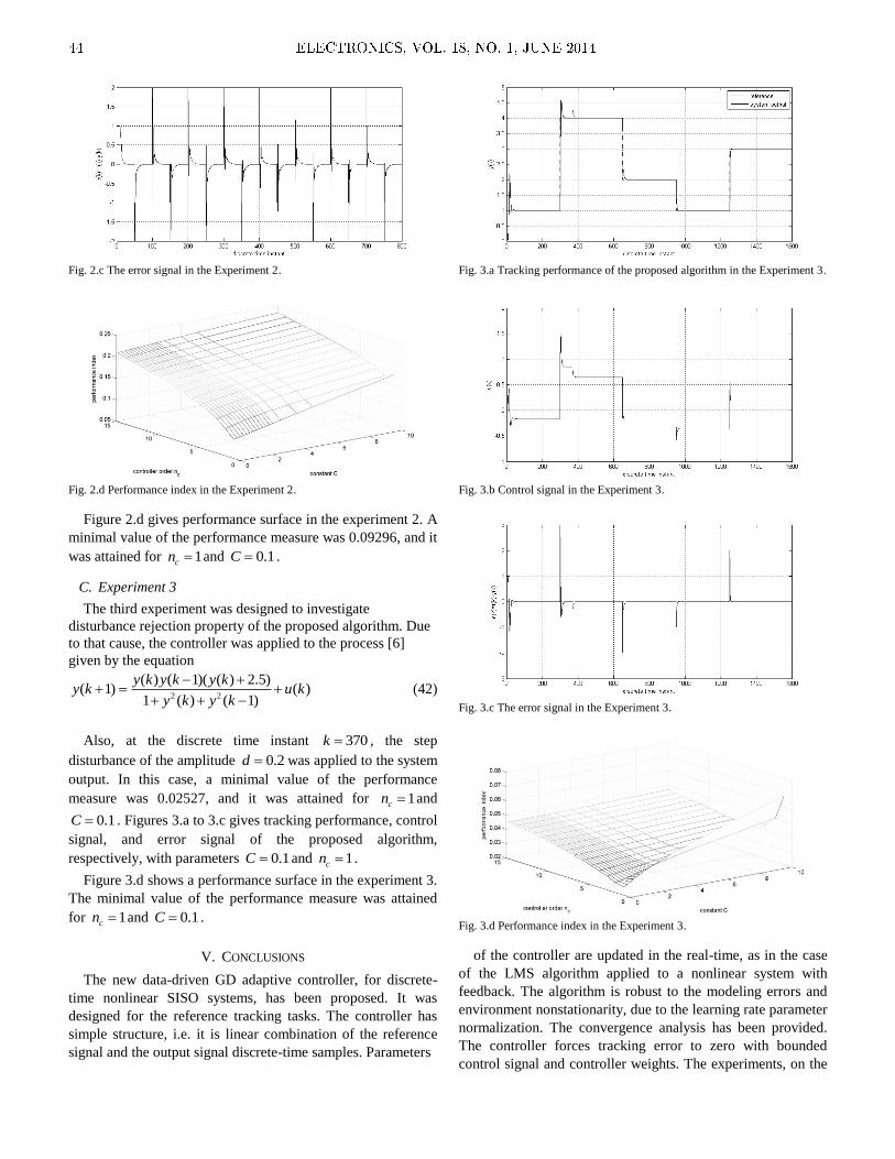
Fig. 2.c The error signal in the Experiment 2.

Fig. 2.d Performance index in the Experiment 2.

Figure 2.d gives performance surface in the experiment 2. A

minimal value of the performance measure was 0.09296, and it

was attained for 1cn and 0.1C .

C. Experiment 3

The third experiment was designed to investigate

disturbance rejection property of the proposed algorithm. Due

to that cause, the controller was applied to the process [6]

given by the equation

2 2

( ) ( 1)( ( ) 2.5)( 1) ( )

1 ( ) ( 1)

y k y k y ky k u k

y k y k

(42)

Also, at the discrete time instant 370k , the step

disturbance of the amplitude 0.2d was applied to the system

output. In this case, a minimal value of the performance

measure was 0.02527, and it was attained for 1cn and

0.1C . Figures 3.a to 3.c gives tracking performance, control

signal, and error signal of the proposed algorithm,

respectively, with parameters 0.1C and 1cn .

Figure 3.d shows a performance surface in the experiment 3.

The minimal value of the performance measure was attained

for 1cn and 0.1C .

V. CONCLUSIONS

The new data-driven GD adaptive controller, for discrete-

time nonlinear SISO systems, has been proposed. It was

designed for the reference tracking tasks. The controller has

simple structure, i.e. it is linear combination of the reference

signal and the output signal discrete-time samples. Parameters

Fig. 3.a Tracking performance of the proposed algorithm in the Experiment 3.

Fig. 3.b Control signal in the Experiment 3.

Fig. 3.c The error signal in the Experiment 3.

Fig. 3.d Performance index in the Experiment 3.

of the controller are updated in the real-time, as in the case

of the LMS algorithm applied to a nonlinear system with

feedback. The algorithm is robust to the modeling errors and

environment nonstationarity, due to the learning rate parameter

normalization. The convergence analysis has been provided.

The controller forces tracking error to zero with bounded

control signal and controller weights. The experiments, on the

44 ELECTRONICS, VOL. 18, NO. 1, JUNE 2014

benchmark systems, demonstrate performance of the proposed

controller and support the analysis.

REFERENCES

[1] Jeffrey T. Spooner, Manfredi Maggiore, Raul Ordonez, and Kevin M.

Passino, Stable Adaptive Control and Estimation for Nonlinear

Systems: Neural and Fuzzy Approximator Techniques, New York: John

Wiley & Sons, Inc., 2002.

[2] M. C. Campi, A. Lecchini, and S. M. Savaresi, “Virtual reference

feedback tuning: a direct method for the design of feedback controllers,”

Automatica, vol. 38, pp. 1337-1346, 2002.

[3] Zhongsheng Hou and Shangtai Jin, “Data-Driven Model-Free Adaptive

Control for a Class of MIMO Nonlinear Discrete-Time Systems,” IEEE

Transactions on Neural Networks, vol. 22, no. 12, pp. 2173-2188, Dec.

2011.

[4] H. Hjalmarsson, S. Gunnarsson, and M. Gevers, “Iterative feedback

tuning: Theory and applications,” IEEE Control System Magazine, vol.

18, no. 4, pp. 26-41, Aug. 1998.

[5] S. Haykin, Neural Networks: A Comprehensive Foundation, Englewood

Cliffs, NJ: Prentice-Hall, 1999.

[6] K. Narendra and K. Parthasarathy, “Identification and control of

dynamical systems using neural networks,” IEEE Transactions on

Neural Networks, vol. 1, pp. 4-27, Jan. 1990.

[7] Hua Deng, Han-Xiong Li, and Yi-Hu Wu, “Feedback-Linearization-

Based Neural Adaptive Control for Unknown Nonaffine Nonlinear

Discrete-Time Systems,” IEEE Transactions on Neural Networks, vol.

19, no. 9, Sep. 2008.

[8] D. Mandic and J. Chambers, Recurrent Neural Networks for Prediction,

New York: Wiley, 2001.

[9] D. P. Mandic, “NNGD algorithm for neural adaptive filters,”

Electronics Letters, vol. 39, no. 6, pp. 845-846, 2000.

[10] Danilo P. Mandic, “A Generalized Normalized Gradient Descent

Algorithm,” IEEE Signal Processing Letters, vol.11, no. 2, pp. 115-118,

Feb. 2004.

[11] D. P. Mandic and I. R. Krcmar, “Stability of NNGD algorithm for

nonlinear system identification,” Electronics Letters, vol. 37, no. 3, pp.

200-202, 2001.

[12] Danilo P. Mandic and Jonathon A. Chambers, “A normalised real time

recurrent learning algorithm,” Signal Processing, vol. 80, pp. 1909-

1916, 2000.

[13] R. J. Williams and D. Zipser, “A learning algorithm for continually

running fully recurrent neural networks,” Neural Computations, vol. 1,

no. 3, pp. 270-280, 1989.

ELECTRONICS, VOL. 18, NO. 1, JUNE 2014 45

Abstract—A modification of the Approximate Internal Model-

based Neural Control (AIMNC), using Multi Layer Neural

Network (MLNN) is introduced. A necessary condition that the

system provides zero steady-state error in case of the constant

reference and constant disturbances is derived. In the considered

control strategy only one neural network (NN), which is the

neural model of the plant, should be trained off-line. An inverse

neural controller can be directly obtained from the neural model

without need for a further training. Simulations demonstrate

performance improvement of the modified AIMNC strategy. An

extension of the modified AIMNC controller for the typical

industrial processes is proposed.

Index Terms—Industrial processes, Neural networks,

Nonlinear internal model control, Zero steady-state error.

Original Research Paper

DOI: 10.7251/ELS1418046I

I. INTRODUCTION

E may imagine an Internal Model Control (IMC)

architecture as a system with two degrees of freedom

consisting of plant model dynamics and some approximation

of the inverse dynamics of the plant model. In this respect the

process as well as its approximate inverse dynamics must be

stable. If the dynamics of the process is not stable, then the

objective of the system design using an IMC approach is,

primarily, stabilization of the process. Such a stabilized system

is then viewed as an equivalent process that must satisfy

forward-mentioned characteristics in terms of stability.

In addition to stability not less important aspect is the

system accuracy. An architecture of the IMC has many

positive characteristics in terms of stability, robustness and

accuracy in a steady-state with respect to one degree of

freedom approaches developed in the area of control

engineering [1],[2].

Manuscript received 13 May 2014. Received in revised form 7 June 2014.

Accepted for publication 11 June 2014.

J. Igic is with the mtel a.d. Banja Luka, Kralja Petra I Karadjordjevica

93, 78.000 Banja Luka, Bosnia and Herzegovina (e-mail:

jasmin.igic@mtel.ba).

M. Bozic is with the University Banja Luka, Faculty of Electrical

Engeneering, Banja Luka, Bosnia and Herzegovina. (e-mail:

mbozic@etfbl.net).

The IMC design algorithms based on linear models have

attracted much attention of control theorists, as well as of

practitioners, especially within industrial applications in

1980s. Almost in parallel with such developments many

successful trials were conducted using the IMC architecture

combined with some kind of adaptation mechanism applied to

control slowly varying processes [3],[4].

Further more, as the MLNN have been proved as universal

approximators they were used in IMC architectures to control

nonlinear processes [2],[5]-[10]. In that sense an Approximate

Internal Model-based Neural Control (AIMNC) and its

modification were proposed for unknown nonlinear discrete

time processes [11]-[13]. High performance of the mentioned

algorithms have been demonstrated at applications to some

benchmark examples of industrial processes. However, we

have noticed unacceptable behavior in applications of such

designs to control slow industrial processes. The typical

industrial processes show some accumulation effects plus dead

time, i.e. they usually have a very slow dynamics.

The well-known examples of such processes are tanks,

where the liquid level is controlled by using the difference

between the input and output flow rates to form a manipulated

variable [14], so in this paper we consider a double tank

system as a plant.

To overcome the above mentioned problem in applications

of the modified AIMNC algorithm, in this paper we present an

extension of the modified AIMNC controller design for slow

nonlinear discrete time processes. This extension is based on a

heuristic consideration of the needed control changes which

provide requested tracking performance of the control system.

However, simulation results confirm the validity of the

proposed control design in cases of slow nonlinear discrete

time processes.

The rest of the paper is organized as follows. In the Section

II, a plant modeling, structure and the modified AIMNC

controller design procedure are given. The Section III gives an

extension of the modified AIMNC algorithm applied to double

tank system together with simulation results demonstrating

performance of the proposed approach in controlling slow

processes. In the Section IV we give conclusions of the work.

A Modified Approximate Internal Model-based

Neural Control for the Typical Industrial

Processes

Jasmin Igic and Milorad Bozic

W

46 ELECTRONICS, VOL. 18, NO. 1, JUNE 2014

II. THE AIMNC CONTROLLER DESIGN

A. The plant modeling

A general input–output representation for an n-dimensional

unknown nonlinear discrete time system with relative degree d

is as follows [15]

)](,[)( kuwfdky k , (1)

where a vector kw is composed of current )(ky and past values

of the output 1,,1),1( niky , and past values of the input

1,,1),1( niku , at the system, and nonlinear mapping is

defined by RRRf nn : with Cf .

Modeling is the first step in designing a controller for

unknown nonlinear system. Different types of neural networks

have been considered for modeling and control of nonlinear

dynamical systems. In this paper, a MLNN has been used for

modeling of nonlinear discrete time dynamical systems due to

its general approximation abilities. If there is an appropriate

number of the neurons in the hidden layers and adequately

determined free parameters, the MLNN can approximate

arbitrary continuous nonlinear function on a compact subset C of nn RR to the desired accuracy [16].

A Neural Network Nonlinear Autoregressive Moving

Average (NARMA) model, i.e. NN NARMA model is defined

as follows [11],[12]

kk kuwNdky )](,[)( , (2)

where ][N is a neural model of the nonlinear dynamical

system and the weight vector of the NN is omitted for

simplicity, k is an output model error.

Taking into account the disturbances acting on the plant, (2)

can be written as

kk vkuwNdky )](,[)( , (3)

where kv represents the effect of uncertainties (model error k

and disturbances).

B. An approximation of the NN model

The NN controller in the IMC control structure represemts

an inversion of the NN model of the plant [7]. Hence, it is

necessary to find the inversion of nonlinear mapping,

represented by the NN, that models the nonlinear plant [2],

[3]. Thus [11]-[13], an approximate model for the system (3)

using Taylor series expansion of )](,[ kuwN k with respect to

)(ku around )1( ku is as

kkkk

kk

vRkukuwNkuwN

vkuwNdky

)()]1(,[)]1(,[

)](,[)(

1

, (4)

where )(/)]1(,[)]1(,[1 kukuwNkuwN kk , )1()()( kukuku ,

and remainder kR is given by

2/))(](,[ 2

2 kuwNR kkk , (5)

where )(/)],[],[ 22

2kuwNwN

kkkk with k as a point

between )(ku and )1( ku .

Based on the assumptions made in [11], after neglecting the

reminder kR and the uncertainty kv in (4), the NN approximate

model output )(ˆ dkym is derived as follows

).()]1(,[)]1(,[)(ˆ1 kukuwNkuwNdky kkm (6)

Since in (6), a control increment )(ku appears linearly in the

output )(ˆ dkym of the NN approximate model, thus the design

of the inverse NN controller is facilitated. To obtain the NN

approximate model (6) and NN controller, the calculation of

)]1(,[1 kuwN k is needed. As was shown in [12], when using the

NN with two hidden layers and neurons with hyperbolic

activation functions within it, both the NN model and a

calculation of )]1(,[1 kuwN k can be obtained by one neural

network, whose parameters are trained off-line.

C. The controller design

From (6) the control increment )(ku is as follows

)].1(,[/)])1(,[)(ˆ()( 1 kuwNkuwNdkyku kkm (7)

The control increment in (6) can be divided into two parts

[12], as shown below

)()()( kukuku cn , (8)

where )(kun refers to the nominal control increment and

)(kuc is used to compensate the model error and

disturbances. Using (8), (6) becomes

)).()()](1(,[

)]1(,[)(ˆ

1 kukukuwN

kuwNdky

cnk

km

(9)

When the model is exact and there is no disturbances, i.e. in

the nominal case, the NN approximate model is given as

follows

).()]1(,[)]1(,[)(ˆ1 kukuwNkuwNdky nkkm (10)

If the NN approximate model given by (10) has a stable

inverse, then the nominal control increment )(kun can be

obtained directly by

)]1(,[/)])1(,[)((

)(

1

kuwNkuwNdkr

ku

kk

n, (11)

ELECTRONICS, VOL. 18, NO. 1, JUNE 2014 47

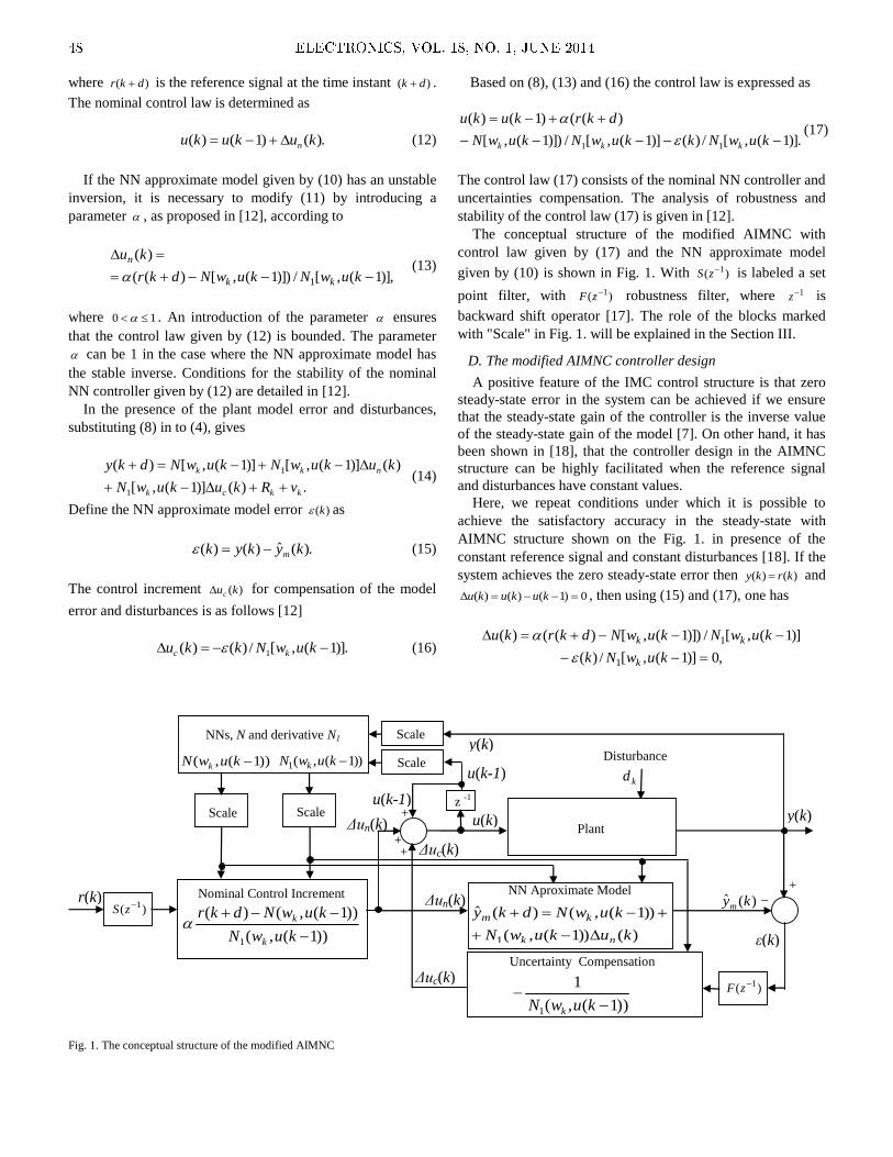
where )( dkr is the reference signal at the time instant )( dk .

The nominal control law is determined as

).()1()( kukuku n (12)

If the NN approximate model given by (10) has an unstable

inversion, it is necessary to modify (11) by introducing a

parameter , as proposed in [12], according to

)],1(,[/)])1(,[)((

)(

1

kuwNkuwNdkr

ku

kk

n

(13)

where 10 . An introduction of the parameter ensures

that the control law given by (12) is bounded. The parameter

can be 1 in the case where the NN approximate model has

the stable inverse. Conditions for the stability of the nominal

NN controller given by (12) are detailed in [12].

In the presence of the plant model error and disturbances,

substituting (8) in to (4), gives

.)()]1(,[

)()]1(,[)]1(,[)(

1

1

kkck

nkk

vRkukuwN

kukuwNkuwNdky

(14)

Define the NN approximate model error )(k as

).(ˆ)()( kykyk m (15)

The control increment )(kuc for compensation of the model

error and disturbances is as follows [12]

)].1(,[/)()( 1 kuwNkku kc (16)

Based on (8), (13) and (16) the control law is expressed as

)].1(,[/)()]1(,[/)])1(,[

)(()1()(

11

kuwNkkuwNkuwN

dkrkuku

kkk

(17)

The control law (17) consists of the nominal NN controller and

uncertainties compensation. The analysis of robustness and

stability of the control law (17) is given in [12].

The conceptual structure of the modified AIMNC with

control law given by (17) and the NN approximate model

given by (10) is shown in Fig. 1. With )( 1zS is labeled a set

point filter, with )( 1zF robustness filter, where 1z is

backward shift operator [17]. The role of the blocks marked

with "Scale" in Fig. 1. will be explained in the Section III.

D. The modified AIMNC controller design

A positive feature of the IMC control structure is that zero

steady-state error in the system can be achieved if we ensure

that the steady-state gain of the controller is the inverse value

of the steady-state gain of the model [7]. On other hand, it has

been shown in [18], that the controller design in the AIMNC

structure can be highly facilitated when the reference signal

and disturbances have constant values.

Here, we repeat conditions under which it is possible to

achieve the satisfactory accuracy in the steady-state with

AIMNC structure shown on the Fig. 1. in presence of the

constant reference signal and constant disturbances [18]. If the

system achieves the zero steady-state error then )()( krky and

0)1()()( kukuku , then using (15) and (17), one has

,0)]1(,[/)(

)]1(,[/)])1(,[)(()(

1

1

kuwNk

kuwNkuwNdkrku

k

kk

y(k)

)(ˆ kym

ε(k)

+ _

u(k)

u(k-1)

z -1

r(k) )( 1zS

)( 1zF

+

+ +

Plant

NN Aproximate Model

)())1(,(

))1(,()(ˆ

1 kukuwN

kuwNdky

nk

km

Uncertainty Compensation

))1(,(

1

1

kuwN k

Nominal Control Increment

))1(,(

))1(,()(

1

kuwN

kuwNdkr

k

k

Δun(k)

NNs, N and derivative N1

Scale

Scale

Δun(k)

u(k-1)

Δuc(k)

Δuc(k)

y(k) Disturbance

kd

))1(,(1 kuwN k ))1(,( kuwN k

Scale

Scale

Fig. 1. The conceptual structure of the modified AIMNC

48 ELECTRONICS, VOL. 18, NO. 1, JUNE 2014

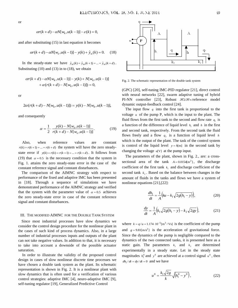
or

,0)()]1(,[)( kkuwNdkr k

and after substituting (15) in last equation it becomes

.0)(ˆ)()]1(,[)( kykykuwNdkr mk (18)

In the steady-state we have )(ˆ...)1(ˆ)(ˆ dkykyky mmm .

Substituting (10) and (13) in to (18), we obtain

,0)])1(,[)((

)]1(,[)()]1(,[)(

kuwNdkr

kuwNkykuwNdkr

k

kk

or

)],1(,[)()])1(,[)((2 kuwNkykuwNdkr kk

and consequently

.)]1(,[)(

)]1(,[)(

2

1

kuwNdkr

kuwNky

k

k (19)

Also, when reference values are constant

)(...)1()( dkrkrkr the system will have the zero steady-

state error if )(...)1()()( dkrkrkrky . It follows from

(19) that 5.0 is the necessary condition that the system in

Fig. 1. attains the zero steady-state error in the case of the

constant reference signal and constant disturbances.

The comparison of the AIMNC strategy with respect to

performance of the fixed and adaptive IMC has been presented

in [18]. Through a sequence of simulations we have

demonstrated performance of the AIMNC strategy and verified

that the system with the parameter value of 5.0 achieves

the zero steady-state error in case of the constant reference

signal and constant disturbances.

III. THE MODIFIED AIMNC FOR THE DOUBLE TANK SYSTEM

Since most industrial processes have slow dynamics we

consider the control design procedure for the nonlinear plant in

the cases of such kind of process dynamics. Also, in a large

number of industrial processes inputs and outputs of the plant

can not take negative values. In addition to that, it is necessary

to take into account a downside of the possible actuator

saturation.

In order to illustrate the validity of the proposed control

design in cases of slow nonlinear discrete time processes we

have chosen a double tank system as the plant. Its schematic

representation is shown in Fig. 2. It is a nonlinear plant with

slow dynamics that is often used for a verification of various

control strategies: adaptive IMC [4], neuro-adaptive IMC [9],

self-tuning regulator [19], Generalized Predictive Control

Fig. 2. The schematic representation of the double tank system

(GPC) [20], self-tuning IMC-PID regulator [21], direct control

with neural networks [22], swarm adaptive tuning of hybrid

PI-NN controller [23], Robust ℋ2/ℋ∞/reference model

dynamic output-feedback control [24].

The input flow q into the first tank is proportional to the

voltage u of the pump P, which is the input to the plant. The

fluid flows from the first tank to the second and flow rate 1q is

a function of the difference of liquid level 1h and h in the first

and second tank, respectively. From the second tank the fluid

flows freely and a flow 2q is a function of liquid level h

which is the output of the plant. The task of the control system

is control of the liquid level ]m[hy in the second tank by

changing the voltage ]V[u at the pump input.

The parameters of the plant, shown in Fig. 2., are: a cross-

sectional area of the tank ]m[0154.0 2A , the discharge

coefficient of the first tank 1k and discharge coefficient of the

second tank 2k . Based on the balance between changes in the

amount of fluids in the tanks and flows we have a system of

nonlinear equations [21],[22]:

yhgkkuAdt

dh 11

1 21

, (20)

gykyhgkAdt

dy22

1211 , (21)

where ]Vs/m[10174.1/ 35 uqk is the coefficient of the pump

and ]9.81[m/s2g is the acceleration of gravitational force.

Since the dynamics of the pump is negligible compared to the

dynamics of the two connected tanks, it is presented here as a

static gain. The parameters 1k and 2k are determined

experimentally in a steady state. Let in the steady state

magnitudes 01h and 0y are achieved at a control signal 0u , then

0//1 dtdydtdh and we have

001

10 2yh

k

gku , (22)

ELECTRONICS, VOL. 18, NO. 1, JUNE 2014 49

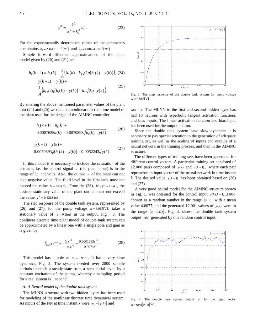
012

221

210 h

kk

ky

. (23)

For the experimentally determined values of the parameters

one obtains ]m[102,46476 2-51 k and ]m[101,816245 2-5

2 k .

Simple forward-difference approximations of the plant

model given by (20) and (21) are

)()(2)(1

)()1( 1111 kykhgkkkuA

khkh , (24)

.)(2)()(2

1

)()1(

211 kygkkykhgkA

kyky

(25)

By entering the above mentioned parameter values of the plant

into (24) and (25) we obtain a nonlinear discrete time model of

the plant used for the design of the AIMNC controller:

,)()(0.0070893)(0007625.0

)()1(

1

11

kykhku

khkh

(26)

.)(0.0052243)()(0.0070893

)()1(

1 kykykh

kyky

(27)

In this model it is necessary to include the saturation of the

actuator, i.e. the control signal u (the plant input) is in the

range of 010 volts. Also, the output y of the plant can not

take negative value. The fluid level in the first tank must not

exceed the value ]m[65.01 h . From the (23), 1.543/ 001 yh , the

desired stationary value of the plant output must not exceed

the value ]m[4213.00 y .

The step response of the double tank system, represented by

(26) and (27), for the pump voltage ]V[065.3u , takes a

stationary value of ]m[2.0y at the output, Fig. 3. The

nonlinear discrete time plant model of double tank system can

be approximated by a linear one with a single pole and gain as

is given by

1

1

11

111

0.99711

0.0001893

1)(

~

z

z

za

zbzPDTS

, (28)

This model has a pole at 9971.01 a . It has a very slow

dynamics, Fig. 3. The system needed over 2000 sample

periods to reach a steady state from a zero initial level, by a

constant excitation of the pump, whereby a sampling period

for a real system is 1 second.

A. A Neural model of the double tank system

The MLNN structure with two hidden layers has been used

for modeling of the nonlinear discrete time dynamical system.

As inputs of the NN at time instant k were )(kywk and

Fig. 3. The step response of the double tank system for pump voltage

]V[065.3u

)1( ku . The MLNN in the first and second hidden layer has

had 10 neurons with hyperbolic tangent activation functions

and bias inputs. The linear activation function and bias input

has been used for the output neuron.

Since the double tank system have slow dynamics it is

necessary to pay special attention to the generation of adequate

training set, as well as the scaling of inputs and outputs of a

neural network in the training process, and then in the AIMNC

structure.

The different types of training sets have been generated for

different control vectors. A particular training set consisted of

12.000 pairs composed of )(ky and )1( ku , where each pair

represents an input vector of the neural network in time instant

k. The desired value )1( ky has been obtained based on (26)

and (27).

A very good neural model for the AIMNC structure shown

in Fig. 1. was obtained for the control input 12000,...,1),( kku

chosen as a random number in the range 80 with a mean

value 4.0077, and the generated 12.001 values of )(ky were in

the range 373.00 . Fig. 4. shows the double tank system

output )(ky generated by this random control input.

Fig. 4. The double tank system output y for the input vector

]V[80randu

50 ELECTRONICS, VOL. 18, NO. 1, JUNE 2014

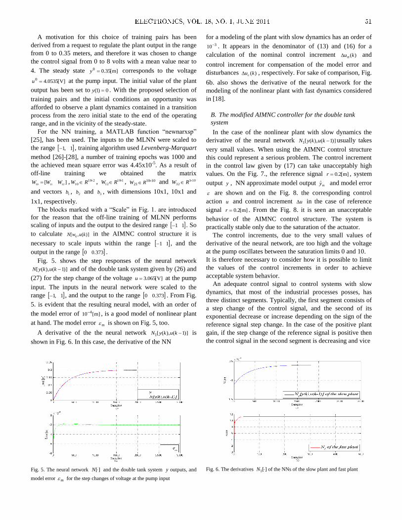
A motivation for this choice of training pairs has been

derived from a request to regulate the plant output in the range

from 0 to 0.35 meters, and therefore it was chosen to change

the control signal from 0 to 8 volts with a mean value near to

4. The steady state ]m[35.00 y corresponds to the voltage

]V[0535.40 u at the pump input. The initial value of the plant

output has been set to 0)1( y . With the proposed selection of

training pairs and the initial conditions an opportunity was

afforded to observe a plant dynamics contained in a transition

process from the zero initial state to the end of the operating

range, and in the vicinity of the steady-state.

For the NN training, a MATLAB function “newnarxsp”

[25], has been used. The inputs to the MLNN were scaled to

the range 1,1 , training algorithm used Levenberg-Marquart

method [26]-[28], a number of training epochs was 1000 and

the achieved mean square error was 4.45x10-5

. As a result of

off-line training we obtained the matrix

][121110

WWW , 21010

RW , 11012

RW , 101021

RW and 10132

RW

and vectors 1b , 2b and 3b , with dimensions 10x1, 10x1 and

1x1, respectively.

The blocks marked with a “Scale” in Fig. 1. are introduced

for the reason that the off-line training of MLNN performs

scaling of inputs and the output to the desired range 11 . So

to calculate )](,[ kuwN k in the AIMNC control structure it is

necessary to scale inputs within the range 11 , and the

output in the range 373.00 .

Fig. 5. shows the step responses of the neural network

)]1(),([ kukyN and of the double tank system given by (26) and

(27) for the step change of the voltage ]V[065.3u at the pump

input. The inputs in the neural network were scaled to the

range 1,1 , and the output to the range 373.00 . From Fig.

5. is evident that the resulting neural model, with an order of

the model error of ]m[10 4 , is a good model of nonlinear plant

at hand. The model error m is shown on Fig. 5, too.

A derivative of the the neural network )]1(),([1 kukyN is

shown in Fig. 6. In this case, the derivative of the NN

Fig. 5. The neural network ][N and the double tank system y outputs, and

model error m for the step changes of voltage at the pump input

for a modeling of the plant with slow dynamics has an order of 310 . It appears in the denominator of (13) and (16) for a

calculation of the nominal control increment )(kun and

control increment for compensation of the model error and

disturbances )(kuc , respectively. For sake of comparison, Fig.

6b. also shows the derivative of the neural network for the

modeling of the nonlinear plant with fast dynamics considered

in [18].

B. The modified AIMNC controller for the double tank

system

In the case of the nonlinear plant with slow dynamics the

derivative of the neural network )]1(),([1 kukyN usually takes

very small values. When using the AIMNC control structure

this could represent a serious problem. The control increment

in the control law given by (17) can take unacceptably high

values. On the Fig. 7., the reference signal ]m[2.0r , system

output y , NN approximate model output my and model error

are shown and on the Fig. 8. the corresponding control

action u and control increment u in the case of reference

signal ]m[2.0r . From the Fig. 8. it is seen an unacceptable

behavior of the AIMNC control structure. The system is

practically stable only due to the saturation of the actuator.

The control increments, due to the very small values of

derivative of the neural network, are too high and the voltage

at the pump oscillates between the saturation limits 0 and 10.

It is therefore necessary to consider how it is possible to limit

the values of the control increments in order to achieve

acceptable system behavior.

An adequate control signal to control systems with slow

dynamics, that most of the industrial processes posses, has

three distinct segments. Typically, the first segment consists of

a step change of the control signal, and the second of its

exponential decrease or increase depending on the sign of the

reference signal step change. In the case of the positive plant

gain, if the step change of the reference signal is positive then

the control signal in the second segment is decreasing and vice

Fig. 6. The derivatives ][1 N of the NNs of the slow plant and fast plant

ELECTRONICS, VOL. 18, NO. 1, JUNE 2014 51

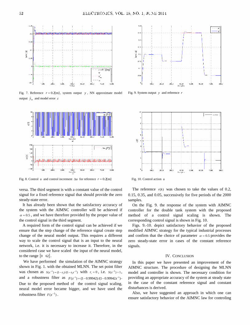
Fig. 7. Reference ]m[2.0r , system output y , NN approximate model

output my and model error

Fig. 8. Control u and control increment u for reference ]m[2.0r

versa. The third segment is with a constant value of the control

signal for a fixed reference signal that should provide the zero

steady-state error.

It has already been shown that the satisfactory accuracy of

the system with the AIMNC controller will be achieved if

5.0 , and we have therefore provided by the proper value of

the control signal in the third segment.

A required form of the control signal can be achieved if we

ensure that the step change of the reference signal create step

change of the neural model output. This requires a different

way to scale the control signal that is an input to the neural

network, i.e. it is necessary to increase it. Therefore, in the

considered case we have scaled the input of the neural model,

to the range 620 .

We have performed the simulation of the AIMNC strategy

shown in Fig. 1. with the obtained MLNN. The set point filter

was chosen as )1/()1()( 111

1 zrrzS with 01r , i.e. 1)( 1 zS ,

and a robustness filter as )0.999421/()0.999421()( 11 zzF .

Due to the proposed method of the control signal scaling,

neural model error became bigger, and we have used the

robustness filter )( 1zF .

Fig. 9. System output y and reference r

Fig. 10. Control action u

The reference )(kr was chosen to take the values of 0.2,

0.15, 0.35, and 0.05, successively for five periods of the 2000

samples.

On the Fig. 9. the response of the system with AIMNC

controller for the double tank system with the proposed

method of a control signal scaling is shown. The

corresponding control signal is shown in Fig. 10.

Figs. 9.-10. depict satisfactory behavior of the proposed

modified AIMNC strategy for the typical industrial processes

and confirm that the choice of parameter 5.0 provides the

zero steady-state error in cases of the constant reference

signals.

IV. CONCLUSION

In this paper we have presented an improvement of the

AIMNC structure. The procedure of designing the MLNN

model and controller is shown. The necessary condition for

providing an appropriate accuracy of the system at steady state

in the case of the constant reference signal and constant

disturbances is derived.

Also, we have suggested an approach in which one can

ensure satisfactory behavior of the AIMNC law for controling

52 ELECTRONICS, VOL. 18, NO. 1, JUNE 2014

slow industrial processes and provide the zero steady state

error in the cases of constant reference signals and constant

disturbances. Simulation results confirm performance

improvements obtained by the proposed modification of the

AIMNC algorithm.

REFERENCES

[1] T.Samad, and A.Annaswamy (Editors), “The Impact of Control

Technology: Overview, Success Stories, and Research Challenges”,

IEEE Control Systems Society, February 2011. Available:

http://ieeecss.org/main/IoCT-report.

[2] K.J.Hunt, and D.Sbarbaro, “Neural networks for nonlinear internal

model control”, IEE Proceedings-D, vol. 138, no. 5, pp. 431-438,

September, 1991.

[3] J. M. Sanches and J. Rodellar, Adaptive Predictive Control: From the

concepts to plant optimization, Prentice Hall, 1996.

[4] J.Igic, M.Bozic, P.Maric, and I.Krcmar, “Adaptive Control based on

Internal Model”, Proc. XLV ETRAN, Conference vol. 1, pp. 209-212,

Bukovicka Banja, June, 2001.

[5] P.M.Mills, A.Y.Zomaya and M.O.Tade, Neuro-Adaptive Process

Control: A Practical Appoach, John Willey&Sons, 1996.

[6] C.Kambhampati, R.J.Craddock, M.Tham, and K.Warwick, “Inverse

model control using recurrent networks”, Mathematics and Computers

in Simulation, vol. 51, pp. 181-199, 2000.

[7] I.Rivals, and L.Personnaz, “Nonlinear internal model control using

neural networks: Application to processes with delay and design

issues,” IEEE Transactions Neural Networks, vol. 11, no. 1, pp.

80–90, January, 2000.

[8] M.Mohammadzaheri, L.Chen, and S.Grainger, ”A critical review of the

most popular types of neuro control”, Asian Journal of Control, vol. 14,

no. 1, pp. 1-11, January 2012.

[9] J.Igic, M.Bozic, and P.Maric, “Neuro-Adaptive Control based on

Internal Model”, Proc. XLVI ETRAN, Conference vol. 1, pp. 161-164,

Banja Vrucica, Teslic, June, 2002.

[10] V.G.Krishnapura, and A.Jutan, “A neural adaptive controller”,

Chemical Engineering Science 55, pp. 3803-3812, 2000.

[11] H.Deng, and H.-X.Li, “A Novel Neural Approximate Inverse Control for

Unknown Nonlinear Discrete Dynamical Systems”, IEEE Transactions

on Systems, Man, and Cybernetics—Part B: Cybernetics, vol. 35, no. 1,

pp. 553-567, February, 2005.

[12] H.-X.Li, and D.Hua, “An Approximate Internal Model-Based Neural

Control for Unknown Nonlinear Discrete Processes,” IEEE

Transactions on Neural Networks, vol. 17, no. 3, pp. 659-670, May,

2006.

[13] Y-N.Wang, and X-F. Yuan, “SVM Approximate-based Internal Model

Control Strategy”, Acta Automatica Sinica, vol. 34, no. 2, pp. 172-179,

February, 2008.

[14] A. Visioli, and Q.-C. Zhong, Control of Integral Processes with Dead

Time. Springer Verlag, London, 2011.

[15] J.B.D. Cabrera, and K.S.Narendra, “Issues in the application of neural

networks for tracking based on inverse control”, IEEE Transactions on.

Automatic Control, vol. 44, no. 11, pp. 2007–2027, November 1999.

[16] M.Sanguineti, “Universal Approximation by Ridge Computational

Models and Neural Networks: A Survey”, The Open Applied

Mathematics Journal, pp. 31-58, 2008.

[17] L.Ljung, System Identification-Theory for the User, 2nd Edition., A

Simon & Schuster Company, N.J., Prentice-Hall PTR, 1999.

[18] J.Igic, and M.Bozic, “An Modified Approximate Internal Model-based

Neural Control”, Proc. XIII INFOTEH Conference, vol.13, pp. 1026–

1031, Jahorina, March, 2014.

[19] J.M.Fernandes, C.E.De Souza, and G.C.Goodwin, "Adaptive Control of

Coupled Tank Apparatus", International Journal of Adaptive Control

and Signal Processing, vol.3, pp.319-331, 1989.

[20] H.Demircioĝlu, and E.Karasu, "Generalized Predictive Control", IEEE

Control Systems Magazine, vol.20, no.5, pp.36-47, October 2000.

[21] W.K.Ho, T.H.Lee, H.P.Han, and Y.Hang, "Self-Tuning IMC-PID

Control with Interval Gain and Phase Margins Assignment" IEEE

Transactions on Control Systems Technology, vol.9, no.3, pp.535-541,

May 2001.

[22] Y.Li, and A.Häuβler, "Artificial Evolution of Neural Networks and its

Application to Feedback Control", Centre for Systems and Control,

University of Glasgow, Tech. Report: CSC-95011, Glasgow, UK, 1995

[23] M. S. Ramli, R. M. T. R. Ismail, M. A. Ahmad, S. M. Nawi, and M. V.

Mat, “Improved Coupled Tank Liquid Levels System Based on Swarm

Adaptive Tuning of Hybrid Proportional-Integral Neural Network

Controller,” Am. J. Eng. Appl. Sci., vol. 2, no. 4, pp. 669–675, 2009.

[24] E. N. Gonçalves, W. E. G. Bachur, R. M. Palhares, and R. H. C.

Takahashi, “Robust ℋ2/ℋ∞/reference model dynamic output-feedback

control synthesis,” Int. J. Control, vol. 84, no. 12, pp. 2067–2080,

November, 2011.

[25] H. Demuth, M. Beale, and M. Hagan, Neural Network Toolbox 6,

User’s Guide. The MathWorks, Inc., 2008.

[26] K. Levenberg, “A method for the solution of certain problems in least

squares,” Quart Appl. Math, vol. 2, pp. 164–168, 1944.

[27] D. W. Marquardt, “An Algorithm for Least-Squares Estimation of

Nonlinear Parameters,” SIAM J. Appl. Math., vol. 11, no. 2, pp. 431–

441, 1963.

[28] J. Nocedal, and S. Wright, Numerical Optimization, 2nd Edition.,

Springer, 2006.

ELECTRONICS, VOL. 18, NO. 1, JUNE 2014 53

Abstract—Distributed generation (DG) has the potential to

bring respectable benefits to electricity customers, distribution

utilities and community in general. Among the customer benefits,

the most important are the electricity bill reduction, reliability

improvement, use of recovered heat, and qualifying for financial

incentives. In this paper, an integrated cost-benefit methodology

for assessment of customer-driven DG is presented. Target

customers are the industrial and commercial end-users that are

critically dependent on electricity supply, due to high

consumption, high power peak demand or high electricity supply

reliability requirements. Stochastic inputs are represented by the

appropriate probability models and then the Monte Carlo

simulation is employed for each investment alternative. The

obtained probability distributions for the prospective profit are

used to assess the risk, compare the alternatives and make

decisions.

Index Terms—Distributed generation (DG), customer-

perspective approach, integrated cost-benefit assessment, Monte

Carlo simulation, long-term planning, uncertainty analysis.

Original Research Paper

DOI: 10.7251/ELS1418054Z

I. INTRODUCTION

N a few recent decades, distributed generation (DG) draws

an increasing attention due to its numerous techno-economic

and environmental potentials [1]. Primarily, the community

may be interested in introducing such a small-scale generation

connected close to end-users in order to improve the overall

efficiency and security of the nation’s energy supply. Second-

ly, distributed generation may bring significant benefits to

distribution power utilities through upgrade investment defer-

ral, avoided electricity purchase, and loss reduction. Finally,

the single electricity customers may also achieve remarkable

benefits from the use of distribution generation especially

through electricity bill reduction, improvement of supply

reliability and combined production of heat and power (CHP).

Manuscript received 31 May 2014. Accepted for publication 10 June

2014. This article partially presents results from the PhD thesis ”Investment

and Operation Aspects of Customer-Driven Distribution Generation under

Uncertainty”, defended at the Faculty of Electrical Engineering, University of

Belgrade.

Čedomir Zeljković is with the Faculty of Electrical Engineering,

University of Banja Luka, Banja Luka, Bosnia and Herzegovina (phone:

+387-51-221-878; e-mail: cedomir@etfbl.net).

Nikola Rajaković is with the School of Electrical Engineering, University

of Belgrade, Belgrade, Serbia (e-mail: rajakovic@etf.rs).

By the most authors, the concept of optimal investment in

distributed generation is considered from the perspective of

distribution power utility. This problem principally comes

down to determination of rated powers and installation

locations for prospective DG units and is usually referred to as

optimal DG sizing and sitting. The optimality criteria are

mainly loss minimization, improvement of reliability and

power quality, network upgrade deferral or voltage profile

improvement [2]-[4]. There are also multi-objective

approaches with a combination of two or more optimization

goals [5]-[7].

Several papers emphasize “a customer approach”, although

the term customers does not refer to electricity end-users, but

to the independent DG developers which consider the

investments in DG units that would be connected at the

appropriate locations in the distribution network being optimal

for investor’s profit maximization. For example, Ref. [8] has

presented a methodology based on the Monte Carlo simulation

where DG units of random size were placed on random

locations in the distribution network searching for the solution

which would offer the maximum overall network benefits. In

the paper is then highlighted that the total achieved benefits

must be accordingly translated to the deserving parties, among

them the DG owners.

On the contrary to the network-perspective approaches, this

paper focuses on the significantly less studied problem of the

benefits achievable by the single electricity customers. In

particular, we deal with the industrial and commercial

customers that are billed by the world’s most common time-of-

use (TOU) electricity tariff, consisted of both volumetric and

demand cost elements. Our target customers observe the

problem exclusively from their point of view and are not in

possession of any data about the structure and operation of the

distribution network they are connected to.

The problem of customer adoption of distributed generation

and optimal operation of installed DG units has been

illustrated in [9]. The optimization task, written in a form of

mixed-integer linear program, has been solved by using

commercial software and, in its original form, has taken into

account only the benefits of electricity bill reduction. This

approach is a pure customer-perspective, though through using

the more general concept of a microgrid, where a group of

related customers are observed together as a low voltage

network. The original model has been extended in [10], where

combined generation of heat as well as the use of local energy

Integrated Cost-Benefit Assessment of

Customer-Driven Distributed Generation

Čedomir Zeljković and Nikola Rajaković

I

54 ELECTRONICS, VOL. 18, NO. 1, JUNE 2014

storage devices have been considered, but still without taking

into account the DG reliability benefits. It is not the only

approach where the potentials of CHP systems to provide

savings to the customers have been analyzed [11][12]. Finally,

in this short literature review, the study of very important issue

of stochastic change of fuel and electricity prices must

necessarily be mentioned [13].

In our previous efforts we have also discussed about the

customer electricity bill reduction by means of the optimal

scheduling of distributed generation. We have introduced a

method based on a search procedure capable of dealing with

non-linear, non-convex and discontinuous DG cost functions

[14]. We have also analyzed the impact of financial incentives

on customer DG investments [15], as well as the potentials of

DG to provide the reliability improvements [16].

In this paper, the results of recent studies have been utilized

in order to establish a new integral DG installation assessment

methodology that would include a majority of influential

factors. The main goal of the methodology is to provide an

answer to the customer is it profitable or not to invest in

distributed generation and which is the best possible solution

from the investment options available on the market. The

approach considers the overall life time of the DG investment

and, due to uncertainties in input parameters, involves not only

deterministic but also stochastic elements. Since the life times

of DG technologies are typically a couple of decades long, the

change in worth of money over time must also be respected

and thus all money amounts must be converted into their

present values. Like in the other long-term planning

methodologies, the employed models and procedures are kept

as simple as possible, but tending to involve all the essential

principles. The main benefits taken into account are the

customer’s bill reduction, reliability improvement, combined

heat and power savings as well as financial incentives. On the

opposite side of the scales lie the DG investment costs. The

probability distributions of net profit calculated from the

benefits and costs are used for declaring the best solution.

They may also be used for the assessment of customer

investment risk. It should be noted that the proposed

methodology is modular and, in case of presence of additional

facts not covered in this study, the new costs/benefits can be

easily attached to the basic framework.

II. PROBLEM FORMULATION AND SOLUTION METHODOLOGY

A. Overview of the System under Consideration

The target customer is a medium or large industrial or

commercial company whose business is significantly

dependent on electricity supply, due to high electricity

consumption, high power peak demand or high electricity

supply reliability requirements. The traditional way for

customer energy supply is purchasing electricity from the

distribution utility company. The alternative is buying fuel

from the market and generating electricity locally, by using

own generating units. The customer considers an investment in

on-site dispatchable generating units such as reciprocating

engines, gas turbines, microturbines, and fuel cells. The

dispatchable units may also be combined with some renewable

energy technologies like solar and wind power devices.

Depending on their rated powers, DG units may partially or

completely satisfy the customer load. A potential deficit can be

compensated by purchasing electricity from the utility. The

purchasing may also be preferred in the case of electricity

prices being more attractive then fuel prices. On the other

hand, it is assumed that the surplus electricity is not sold back

to the grid. The opposite class of problems, assuming the two-

way flow of energy and net-metering, deserves its own

approach. Finally, since our research is focused on the

application of distributed generation, the other customer cost-

saving techniques like demand-side management or local

energy storage are not considered in the paper. The concept of

the system is illustrated in Fig. 1.

POWER UTILITY

L1

L2

L3

Lm

CONTROL

G1

Gn

DG UNITS

LOADS

ENERGY STORAGE (optional)

Fig. 1. The concept of the system under consideration

B. Stochastic vs. Deterministic Methodology

In case when all inputs are known with complete certainty,

the economic cost-benefit assessment may be performed using

the traditional discounted cash flow (DCF) method [17]. For

each considered investment alternative, the net present value

(NPV) is calculated using the following manner

Lkk

kjkj

jd

CBNPV

1

,,

where Bj,k is the benefit obtained by the use of DG investment

alternative j during the year k, Cj,k is the corresponding

annualized cost, d is the discount rate and L is the life time of

the investment. The usual decision-making approach is

choosing the alternative having the highest positive NPV.

On the contrary, in cases when several input variables

exhibit stochastic changes, the conventional approach should

be extended. One of the most comprehensive methods for

analyzing problems that involve uncertainty is Monte Carlo

simulation (MCS) [18]. In the MCS method, the main

stochastic variables are assigned probabilistic models, a

sufficient number of random scenarios is generated and, for

each scenario, the behavior of the system is simulated. The

output of MCS procedure is a probability distribution of NPV,

which represents a full spectrum of possible outcomes of the

ELECTRONICS, VOL. 18, NO. 1, JUNE 2014 55

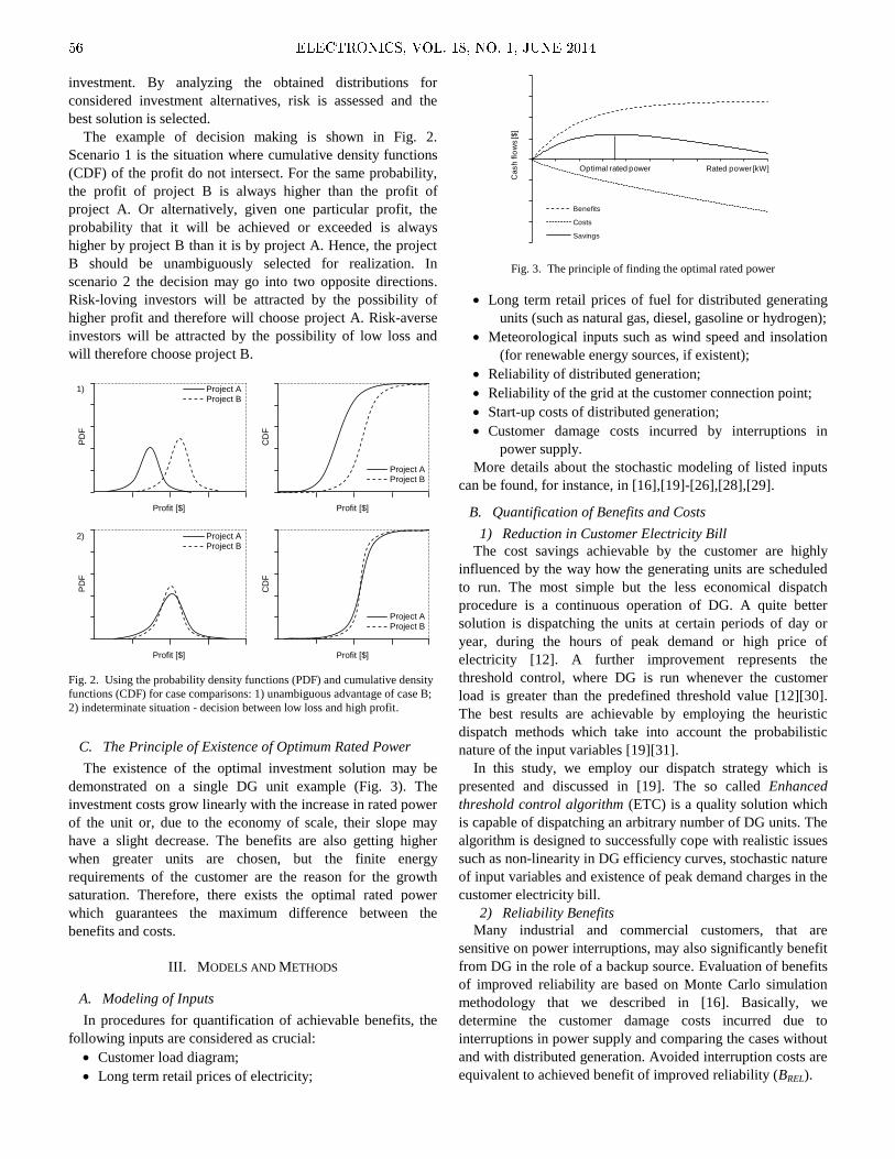
investment. By analyzing the obtained distributions for

considered investment alternatives, risk is assessed and the

best solution is selected.

The example of decision making is shown in Fig. 2.

Scenario 1 is the situation where cumulative density functions

(CDF) of the profit do not intersect. For the same probability,

the profit of project B is always higher than the profit of

project A. Or alternatively, given one particular profit, the

probability that it will be achieved or exceeded is always

higher by project B than it is by project A. Hence, the project

B should be unambiguously selected for realization. In

scenario 2 the decision may go into two opposite directions.

Risk-loving investors will be attracted by the possibility of

higher profit and therefore will choose project A. Risk-averse

investors will be attracted by the possibility of low loss and

will therefore choose project B.

PD

F

Profit [$]

Project A Project B

1)

CD

F

Profit [$]

Project A Project B

PD

F

Profit [$]

Project A Project B

2)

CD

F

Profit [$]

Project A Project B

Fig. 2. Using the probability density functions (PDF) and cumulative density

functions (CDF) for case comparisons: 1) unambiguous advantage of case B;

2) indeterminate situation - decision between low loss and high profit.

C. The Principle of Existence of Optimum Rated Power

The existence of the optimal investment solution may be

demonstrated on a single DG unit example (Fig. 3). The

investment costs grow linearly with the increase in rated power

of the unit or, due to the economy of scale, their slope may

have a slight decrease. The benefits are also getting higher

when greater units are chosen, but the finite energy

requirements of the customer are the reason for the growth

saturation. Therefore, there exists the optimal rated power

which guarantees the maximum difference between the

benefits and costs.

III. MODELS AND METHODS

A. Modeling of Inputs

In procedures for quantification of achievable benefits, the

following inputs are considered as crucial:

Customer load diagram;

Long term retail prices of electricity;

Cash

flo

ws

[$]

Rated power [kW]

Benefits

Costs

Savings

Optimal rated power

Fig. 3. The principle of finding the optimal rated power

Long term retail prices of fuel for distributed generating

units (such as natural gas, diesel, gasoline or hydrogen);

Meteorological inputs such as wind speed and insolation

(for renewable energy sources, if existent);

Reliability of distributed generation;

Reliability of the grid at the customer connection point;

Start-up costs of distributed generation;

Customer damage costs incurred by interruptions in

power supply.

More details about the stochastic modeling of listed inputs

can be found, for instance, in [16],[19]-[26],[28],[29].

B. Quantification of Benefits and Costs

1) Reduction in Customer Electricity Bill

The cost savings achievable by the customer are highly

influenced by the way how the generating units are scheduled

to run. The most simple but the less economical dispatch

procedure is a continuous operation of DG. A quite better

solution is dispatching the units at certain periods of day or

year, during the hours of peak demand or high price of

electricity [12]. A further improvement represents the

threshold control, where DG is run whenever the customer

load is greater than the predefined threshold value [12][30].

The best results are achievable by employing the heuristic

dispatch methods which take into account the probabilistic

nature of the input variables [19][31].

In this study, we employ our dispatch strategy which is

presented and discussed in [19]. The so called Enhanced

threshold control algorithm (ETC) is a quality solution which

is capable of dispatching an arbitrary number of DG units. The

algorithm is designed to successfully cope with realistic issues

such as non-linearity in DG efficiency curves, stochastic nature

of input variables and existence of peak demand charges in the

customer electricity bill.

2) Reliability Benefits

Many industrial and commercial customers, that are

sensitive on power interruptions, may also significantly benefit

from DG in the role of a backup source. Evaluation of benefits

of improved reliability are based on Monte Carlo simulation

methodology that we described in [16]. Basically, we

determine the customer damage costs incurred due to

interruptions in power supply and comparing the cases without

and with distributed generation. Avoided interruption costs are

equivalent to achieved benefit of improved reliability (BREL).

56 ELECTRONICS, VOL. 18, NO. 1, JUNE 2014

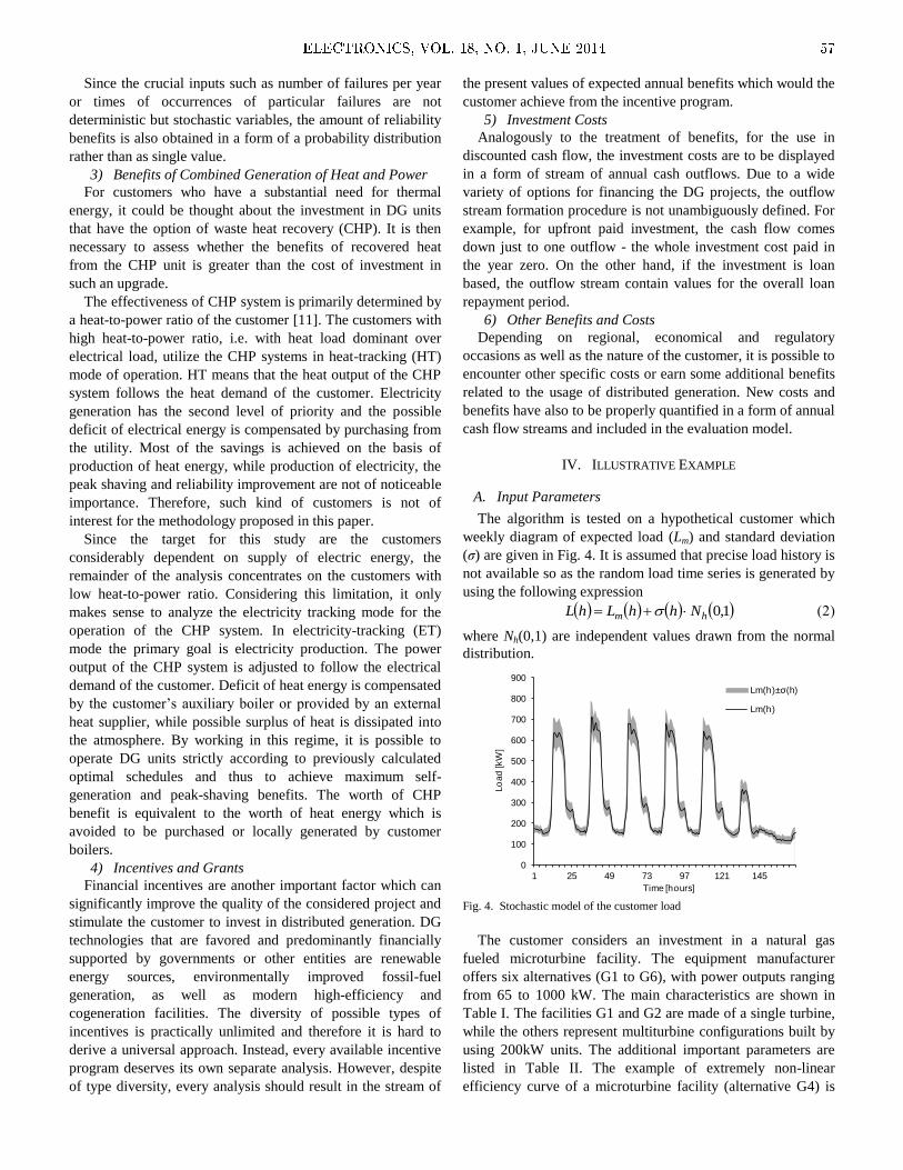
Since the crucial inputs such as number of failures per year

or times of occurrences of particular failures are not

deterministic but stochastic variables, the amount of reliability

benefits is also obtained in a form of a probability distribution

rather than as single value.

3) Benefits of Combined Generation of Heat and Power

For customers who have a substantial need for thermal

energy, it could be thought about the investment in DG units

that have the option of waste heat recovery (CHP). It is then

necessary to assess whether the benefits of recovered heat

from the CHP unit is greater than the cost of investment in

such an upgrade.

The effectiveness of CHP system is primarily determined by

a heat-to-power ratio of the customer [11]. The customers with

high heat-to-power ratio, i.e. with heat load dominant over

electrical load, utilize the CHP systems in heat-tracking (HT)

mode of operation. HT means that the heat output of the CHP

system follows the heat demand of the customer. Electricity

generation has the second level of priority and the possible

deficit of electrical energy is compensated by purchasing from

the utility. Most of the savings is achieved on the basis of

production of heat energy, while production of electricity, the

peak shaving and reliability improvement are not of noticeable

importance. Therefore, such kind of customers is not of

interest for the methodology proposed in this paper.

Since the target for this study are the customers

considerably dependent on supply of electric energy, the

remainder of the analysis concentrates on the customers with

low heat-to-power ratio. Considering this limitation, it only

makes sense to analyze the electricity tracking mode for the

operation of the CHP system. In electricity-tracking (ET)

mode the primary goal is electricity production. The power

output of the CHP system is adjusted to follow the electrical

demand of the customer. Deficit of heat energy is compensated

by the customer’s auxiliary boiler or provided by an external

heat supplier, while possible surplus of heat is dissipated into

the atmosphere. By working in this regime, it is possible to

operate DG units strictly according to previously calculated

optimal schedules and thus to achieve maximum self-

generation and peak-shaving benefits. The worth of CHP

benefit is equivalent to the worth of heat energy which is

avoided to be purchased or locally generated by customer

boilers.

4) Incentives and Grants

Financial incentives are another important factor which can

significantly improve the quality of the considered project and

stimulate the customer to invest in distributed generation. DG

technologies that are favored and predominantly financially

supported by governments or other entities are renewable

energy sources, environmentally improved fossil-fuel

generation, as well as modern high-efficiency and

cogeneration facilities. The diversity of possible types of

incentives is practically unlimited and therefore it is hard to

derive a universal approach. Instead, every available incentive

program deserves its own separate analysis. However, despite

of type diversity, every analysis should result in the stream of

the present values of expected annual benefits which would the

customer achieve from the incentive program.

5) Investment Costs

Analogously to the treatment of benefits, for the use in

discounted cash flow, the investment costs are to be displayed

in a form of stream of annual cash outflows. Due to a wide

variety of options for financing the DG projects, the outflow

stream formation procedure is not unambiguously defined. For

example, for upfront paid investment, the cash flow comes

down just to one outflow - the whole investment cost paid in

the year zero. On the other hand, if the investment is loan

based, the outflow stream contain values for the overall loan

repayment period.

6) Other Benefits and Costs

Depending on regional, economical and regulatory

occasions as well as the nature of the customer, it is possible to

encounter other specific costs or earn some additional benefits

related to the usage of distributed generation. New costs and

benefits have also to be properly quantified in a form of annual

cash flow streams and included in the evaluation model.

IV. ILLUSTRATIVE EXAMPLE

A. Input Parameters

The algorithm is tested on a hypothetical customer which

weekly diagram of expected load (Lm) and standard deviation

(σ) are given in Fig. 4. It is assumed that precise load history is

not available so as the random load time series is generated by

using the following expression

1,0hm NhhLhL

where Nh(0,1) are independent values drawn from the normal

distribution.

0

100

200

300

400

500

600

700

800

900

1 25 49 73 97 121 145

Lo

ad

[kW

]

Time [hours]

Lm(h)±σ(h)

Lm(h)

Fig. 4. Stochastic model of the customer load

The customer considers an investment in a natural gas

fueled microturbine facility. The equipment manufacturer

offers six alternatives (G1 to G6), with power outputs ranging

from 65 to 1000 kW. The main characteristics are shown in

Table I. The facilities G1 and G2 are made of a single turbine,

while the others represent multiturbine configurations built by

using 200kW units. The additional important parameters are

listed in Table II. The example of extremely non-linear

efficiency curve of a microturbine facility (alternative G4) is

ELECTRONICS, VOL. 18, NO. 1, JUNE 2014 57

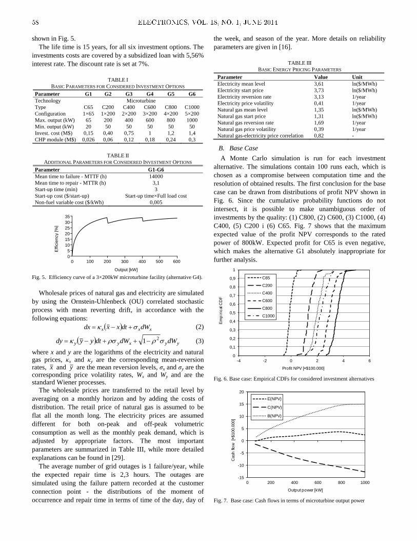
shown in Fig. 5.

The life time is 15 years, for all six investment options. The

investments costs are covered by a subsidized loan with 5,56%

interest rate. The discount rate is set at 7%.

TABLE I

BASIC PARAMETERS FOR CONSIDERED INVESTMENT OPTIONS

Parameter G1 G2 G3 G4 G5 G6

Technology Microturbine

Type C65 C200 C400 C600 C800 C1000

Configuration 1×65 1×200 2×200 3×200 4×200 5×200

Max. output (kW) 65 200 400 600 800 1000

Min. output (kW) 20 50 50 50 50 50

Invest. cost (M$) 0,15 0,40 0,75 1 1,2 1,4

CHP module (M$) 0,026 0,06 0,12 0,18 0,24 0,3

TABLE II

ADDITIONAL PARAMETERS FOR CONSIDERED INVESTMENT OPTIONS

Parameter G1-G6

Mean time to failure - MTTF (h) 14000

Mean time to repair - MTTR (h) 3,1

Start-up time (min) 3

Start-up cost ($/start-up) Start-up time×Full load cost

Non-fuel variable cost ($/kWh) 0,005

Effic

iency [%

]

Output [kW]

0 400 200 600 300 100 500 0

5

10

15

20

25

30

35

Fig. 5. Efficiency curve of a 3×200kW microturbine facility (alternative G4).

Wholesale prices of natural gas and electricity are simulated

by using the Ornstein-Uhlenbeck (OU) correlated stochastic

process with mean reverting drift, in accordance with the

following equations:

xxx dWdtxxdx (2)

yyxyy dWdWdtyydy 21 (3)

where x and y are the logarithms of the electricity and natural gas prices, κx and κy are the corresponding mean-reversion rates, x and y are the mean reversion levels, σx and σy are the corresponding price volatility rates, Wx and Wy and are the standard Wiener processes.

The wholesale prices are transferred to the retail level by

averaging on a monthly horizon and by adding the costs of

distribution. The retail price of natural gas is assumed to be

flat all the month long. The electricity prices are assumed

different for both on-peak and off-peak volumetric

consumption as well as the monthly peak demand, which is

adjusted by appropriate factors. The most important

parameters are summarized in Table III, while more detailed

explanations can be found in [29].

The average number of grid outages is 1 failure/year, while

the expected repair time is 2,3 hours. The outages are

simulated using the failure pattern recorded at the customer

connection point - the distributions of the moment of

occurrence and repair time in terms of time of the day, day of

the week, and season of the year. More details on reliability

parameters are given in [16].

TABLE III

BASIC ENERGY PRICING PARAMETERS

Parameter Value Unit

Electricity mean level 3,61 ln($/MWh)

Electricity start price 3,73 ln($/MWh)

Electricity reversion rate 3,13 1/year

Electricity price volatility 0,41 1/year

Natural gas mean level 1,35 ln($/MWh)

Natural gas start price 1,31 ln($/MWh)

Natural gas reversion rate 1,69 1/year

Natural gas price volatility 0,39 1/year

Natural gas-electricity price correlation 0,82 -

B. Base Case

A Monte Carlo simulation is run for each investment

alternative. The simulations contain 100 runs each, which is

chosen as a compromise between computation time and the

resolution of obtained results. The first conclusion for the base

case can be drawn from distributions of profit NPV shown in

Fig. 6. Since the cumulative probability functions do not

intersect, it is possible to make unambiguous order of

investments by the quality: (1) C800, (2) C600, (3) C1000, (4)

C400, (5) C200 i (6) C65. Fig. 7 shows that the maximum

expected value of the profit NPV corresponds to the rated

power of 800kW. Expected profit for C65 is even negative,

which makes the alternative G1 absolutely inappropriate for

further analysis.

0

0,1

0,2

0,3

0,4

0,5

0,6

0,7

0,8

0,9

1

-4 -2 0 2 4 6

Em

pir

ical

CD

F

Profit NPV [ $100.000]

C65

C200

C400

C600

C800

C1000

Fig. 6. Base case: Empirical CDFs for considered investment alternatives

-15

-10

-5

0

5

10

15

20

0 200 400 600 800 1000

Cash

flo

w [

$100.0

00]

Output power [kW]

E(NPV)

C(NPV)

B(NPV)

Fig. 7. Base case: Cash flows in terms of microturbine output power

58 ELECTRONICS, VOL. 18, NO. 1, JUNE 2014

C. Sensitivity Analysis

Errors in the input parameters may lead to erroneous results

and conclusions. Therefore, the analysis is performed in order

to determine how the results are influenced by the change in

particular inputs. In this paper we show some representative

results of our comprehensive sensitivity analysis. The

investigation is limited to three most promising alternatives,

namely G4-G6.

1) Case A: Electricity Price Volatility

Case A covers the impact of electricity price volatility. Fig.

8 shows that the increase in volatility of approximately 50%

leads to a just slight increase in profit NPV, for each

investment alternative. The increase is logical since the greater

deviation in electricity price provides room for distributed

generation to participate more effectively both in peak shaving

and energy generation. Fig. 9 shows that the increase in

deviation of the electricity price also leads to the larger

deviation of the profit NPV. Obviously, C800 remains the best

alternative for the customer.

-15

-10

-5

0

5

10

15

20

0 200 400 600 800 1000

Cash

flo

ws [

$100.0

00]

Output power [kW]

E(NPV)

C(NPV)

B(NPV)

Fig. 8. Case A: Cash flows in terms of microturbine output power

2

2,5

3

3,5

4

0,3 0,4 0,5 0,6 0,7 0,8

Exp

ecte

d N

PV

[×$100.0

00]

Standard deviation [×$100.000]

a) Electricity price volatility: 0,41 -> 0,6G4

G5

G6

G4a

G5a

G6a

Fig. 9. Case A: Changes in expected value and standard deviation of profit

NPV due to increase in electricity price volatility.

2) Case B: Natural Gas to Electricity Price Correlation

In the base case, the correlation between the prices of

natural gas and electricity is assumed to be high, which is

appropriate for the markets where a large portion of electricity

is produced by gas power plants. The adopted value of the

correlation coefficient ρ in the formula (3) is 0,82. In this

analysis, the initial value of the correlation coefficient is

decreased down to ρ = 0,41. Fig. 10 shows that halving the

correlation factor significantly affects the standard deviation of

NPV, while the expected values are left almost unchanged.

The interpretation of this phenomenon is simple. When the

prices of gas and electricity change with the correlated

trajectories, the ratio of their prices are not changed within

wide limits, so the customer savings are similar from month to

month. When the correlation decreases, the ratio of the price

of gas and electricity oscillates more. Therefore, in cases with

expensive electricity the savings are getting greater and in

cases with expensive gas the savings are getting lower. This

increases the deviation of the results, but the average value of

the profit does not experience a remarkable change.

2

2,5

3

3,5

4

0,3 0,4 0,5 0,6 0,7 0,8

Exp

ecte

d N

PV

[×$100.0

00]

Standard deviation [×$100.000]

b) Electricity-gas price correlation 0,82 -> 0.41G4

G5

G6

G4b

G5b

G6b

Fig. 10. Case B: Changes in expected value and standard deviation of profit

NPV due to decrease in correlation between the prices of natural gas and

electricity.

3) Case C: Natural Gas to Electricity Mean Level Ratio

The gas/electricity price ratio is one of the most important

factors that dictate the amount of achievable savings for the

customer. Case C will test the impact of this variable. The

mean level of natural gas price logarithm is therefore changed

from initial 1,35 to an arbitrary new value of 1,54. As might be

expected, the impact on the achievable savings will be very

strong. Because of the expensive gas, distributed generation

will be used much rarely, mainly just for the peak shaving.

Results in Fig. 11 show that the alternative with C1000 very

likely finishes its life time with negative NPV of the profit.

The alternatives C600 and C800 keep the profits positive, but

the expected values of NPV are more than halved in

comparison with the base case. Once again, C800 remains the

best investment alternative.

0

0,1

0,2

0,3

0,4

0,5

0,6

0,7

0,8

0,9

1

-4 -2 0 2 4 6

Em

pir

ical

CD

F

Profit NPV [ $100.000]

C600

C800

C1000

Fig. 11. Case C: Empirical CDFs for considered investment alternatives.

ELECTRONICS, VOL. 18, NO. 1, JUNE 2014 59

4) Case D: Load deviation

Case D covers the influence of uncertainty in customer load

to the amount of savings achievable by DG. The standard

deviation of the customer load from the base case is doubled

here and the Monte Carlo simulations are performed again for

the alternatives G4-G6. Increased deviation of the load

logically leads to an increase in the monthly peak demand.

Therefore, C1000 comes into play since it has the largest

potential for the peak shaving. As per Fig. 12 the overall

performance of C1000 almost reaches the results achievable

by C800. C600 as the facility with the smallest output power is

not significantly affected by the change in the load deviation.

2

2,5

3

3,5

4

0,3 0,4 0,5 0,6 0,7 0,8

Exp

ecte

d N

PV

[×$100.0

00]

Standard deviation [×$100.000]

d) Load deviation: 1x -> 2xG4

G5

G6

G4d

G5d

G6d

Fig. 12. Case D: Changes in expected value and standard deviation of profit

NPV due to increase in deviation of the customer load.

D. Contribution in Reliability Improvement

It is interesting to determine which portion of the total

benefits is related to improved reliability. According to

principles described in [16], the customer loads are sorted in a

priority order, so as in case of the grid outage, the most critical

loads are served first by distributed generation. Although the

less critical loads are left disconnected, the customer does not

incur a significant additional damage. For the customer

considered in this paper, microturbine facility C600 with

600kW rated power is sufficient to cover the most critical

loads. Therefore, C800 and C1000 with their surplus of output

power are not worth much in terms of reliability. Fig. 13

illustrates that the benefits of improved reliability are

practically the same for each investment alternative. The

expected present value of reliability benefits are about 16,5%

of the overall customer benefits. With modifications of input

parameters defined in cases A to D, the results obtained for the

base case are not significantly changed.

E. Final Decision Based on Power Aspects

Using the results of presented comprehensive analysis, the

customer would select the alternative based on C800

microturbine facility. This alternative shows the best results

for the wide range of change in crucial input parameters. The

risk of loss (i.e. negative profit NPV) is negligible.

The customer primarily benefits on cutting costs for energy

supply. The benefits of improved reliability are just 1/6 of the

total benefits. It should be noted that the ratio between

particular benefits can be significantly changed under different

conditions. For example, for the customers connected to

unreliable distribution grid, the benefits of improved reliability

can be even greater than the benefits of cheaper energy supply.

0

0,1

0,2

0,3

0,4

0,5

0,6

0,7

0,8

0,9

1

-4 -2 0 2 4 6

Em

pir

ical

CD

F

PV(Brel) [×$100.000]

C600

C800

C1000

Fig. 13. Base case: Contribution of reliability improvement to the total profit

NPV

F. Combined Heat and Power

Microturbine exhaust gases contain a respectable amount of

heat energy. Heat to power ratio for microturbine technology

is regularly greater than 1,5. By investing in a system of heat

exchangers, available heat energy might be used for space

heating, water heating, etc. It depends on the nature of the

customer how much of the available heat can be effectively

utilized.

We tested how much heat energy is available for six

investment alternatives (G1–G6), while the microturbines are

dispatched according to the proposed ETC algorithm. It is

assumed that the customer used their own boiler to produce

heat, prior to the investment in distributed generation. Natural

gas is bough at the retail prices, as same as for microturbine

purposes. The boiler efficiency is set to 80%. We calculated

the amount of avoided purchase of natural gas thanks to the

use of heat recovered from the microturbines. The heat

exchanger investment costs are deducted from the value of

benefit in order to compute the net profit of the investment.

Fig. 14 shows that the upgrade in CHP has a huge

theoretical maximum potential. If total available heat energy

would be utilized, the investment in CHP would be very

profitable. On the other hand, it is not easy to achieve a perfect

matching between the load profiles of electricity and heat. In a

simple case of space heating, the available heat would be used

only during the colder months.

-15

-10

-5

0

5

10

15

20

0 200 400 600 800 1000

Cash

flo

ws [

$100,0

00]

Electrical output [kW]

Heat benefit

Heat profit NPV

Heat exchanger cost

Fig. 14. Cost-effectiveness of investment in microturbine heat exchangers

60 ELECTRONICS, VOL. 18, NO. 1, JUNE 2014

In order to precisely calculate the benefits of recovered heat,

a detailed model of customer heat load profile is necessary. In

this paper, we determine just the profitability thresholds

expressed as a percentage of the theoretical maximum, where

the investment in CHP upgrade is still profitable for the

customer. The results are summarized in Table IV.

It should be noted that the investments in CHP can be

subsidized under certain circumstances, which would

additionally lower the profitability thresholds.

TABLE IV

PROFITABILITY THRESHOLDS FOR INVESTMENT IN CHP UPGRADE

Unit C65 C200 C400

CHP investment cost NPV ×105$ 0,24 0,55 1,09

Benefit NPV ×105$ 2,79 5,44 7,76

Profitability threshold % 8,5 10,1 14,1

Unit C600 C800 C1000

CHP investment cost NPV ×105$ 1,64 2,19 2,73

Benefit NPV ×105$ 9,61 10,98 11,02

Profitability threshold % 17,1 19,9 24,8

V. CONCLUSION

In this paper the profitability of investing in customer-driven

distributed generation has been considered. The target

customers are industrial and commercial users of electricity,

which are billed not only for the volumetric consumption but

also for the monthly peak demand. Presented methodology is

capable of providing the answer whether or not it is profitable

to invest in distributed generation, and which is the most

appropriate investment option for the customer. The proposed

methodology has been comprehensively tested on one

integrated illustrative example.

REFERENCES

[1] G. Pepermans, J. Driesen, D. Haeseldonckx, R. Belmans, and W.

D’haeseleer, "Distributed generation: definition, benefits and issues",

Energy Policy, vol. 33, pp. 787-798, 2005.

[2] A. A. Chowdhury, S. K. Agarwal, and D. O. Koval, "Reliability

modeling of distributed generation in conventional distribution systems

planning and analysis", IEEE Transactions on Industry Applications,

vol. 39, pp. 1493-1498, 2003.

[3] A. Moreno-Munoz, J. J. G. de-la-Rosa, M. A. Lopez-Rodriguez, J. M.

Flores-Arias, F. J. Bellido-Outerino, and M. Ruiz-de-Adana,

"Improvement of power quality using distributed generation",

International Journal of Electrical Power Energy Systems, vol. 32 pp.

1069-1076, 2010.

[4] H. A. Gil and G. Joos, "On the quantification of the network capacity

deferral value of distributed generation", IEEE Transactions on Power

Systems, vol. 21, pp. 1592-1599, 2006.

[5] H. A. Gil and G. Joos, "Models for quantifying the economic benefits of

distributed generation", IEEE Transactions on Power Systems, vol. 23

pp. 327-335, 2008.

[6] I. -S. Bae, J. O. Kim, J. -C. Kim and C. Singh, "Optimal operating

strategy for distributed generation considering hourly reliability worth",

IEEE Transactions on Power Systems, vol. 19, pp. 287-292, 2004.

[7] A. Barina, L. F. Pozzatti, L. N. Canha, R. Q. Machado, A. R. Abaide,

and G. Arend, "Multi-objective analysis of impacts of distributed

generation placement on the operational characteristics of networks for

distribution system planning", International Journal of Electrical

Power Energy Systems, vol. 32, pp. 1157-1164, 2010.

[8] M. Zangiabadi, R. Feuillet, H. Lesani, N. Hadj-Said, and J. T. Kvaløy,

"Assessing the performance and benefits of customer distributed

generation developers under uncertainties", Energy, vol. 36, pp. 1703-

1712, 2011.

[9] C. Marnay, J. Chard, K. Hamachi, T. Lipman, M. Moezzi, B. Ouaglal,

and A.Siddiqui, "Modeling of customer adoption of distributed energy

resources", Lawrence Berkeley National Laboratory Report LBNL-

49582, Berkeley, CA, USA, 2001.

[10] A. S. Siddiqui, C. Marnay, R. M. Firestone, and N. Zhou, "Distributed

generation with heat recovery and storage", Journal of Energy

Engineering, vol. 133, pp. 181-210, 2007.

[11] Y. Ruan, Q. Liu, W. Zhou, R. Firestone, W. Gao, and T. Watanabe,

"Optimal option of distributed generation technologies for various

commercial buildings", Applied Energy, vol. 86, pp. 1641-1653, 2009.

[12] B. Coffey and E. Kutrowski, "Demand charge considerations in the

optimization of cogeneration dispatch in a deregulated energy market",

International Journal of Energy Research, vol. 30, pp. 535-551, 2006.

[13] A. S. Siddiqui and C. Marnay, "Distributed generation investment by a

microgrid under uncertainty", Energy, vol. 33, pp. 1729-1737, 2008.

[14] Č. V. Zeljković, N. Lj. Rajaković, and S. J. Zubić, "A method for cost

minimization applicable to load centers containing distributed

generation", in Proc. IEEE PowerTech Conf., Bucharest Romania, June

28 – July 2, 2009, pp. 1-6.

[15] Č. V. Zeljković, N. Lj. Rajaković, and S. J. Zubić, "An application of

cost minimization algorithm to economic justification of installing

distributed generation", in Proc. IFAC CMTEE Conference Vilamoura,

Portugal, March 29-31, 2010, pp. 243-248.

[16] Č. V. Zeljković, N. Lj. Rajaković, and S. J. Zubić, "Customer-

perspective approach to reliability evaluation of distributed generation",

in Proc. IEEE PowerTech Conf., Trondheim Norway, June 19-23, 2011.

[17] R. A. Brealey and S. C. Myers, Principles of corporate finance, 7th ed.,

Boston: McGraw-Hill, 2003.

[18] S. C. Savvides, “Risk analysis in investment appraisal”, Project

Appraisal, vol. 9, pp. 3-18, 1994.

[19] Č. Zeljković and N. Rajaković, “Cost-saving potential of customer-

driven distributed generation,” Electric Power Systems Research, vol.

92, pp. 87-95, 2012.

[20] J. Nowicka-Zagrajek and R. Weron, "Modeling electricity loads in

California: ARMA models with hyperbolic noise", Signal Processing,

vol. 82, pp. 1903-1915, 2002.

[21] B. Klöckl, G. Papaefthymiou, Multivariate time series models for

studies on stochastic generators in power systems, Electr.Power Syst.

Res. 80 (2010) 265-276.

[22] G. H. Kjølle, and A. T. Holen, Reliability and interruption cost

prediction using time-dependent failure rates and interruption costs,

Qual. Reliab. Eng. Int.14 (1998) 159-165.

[23] R. Billinton W. Li, Reliability Assessment of electric power systems

using Monte Carlo methods, New York: Plenum, 1994.

[24] L. Goel, X. Liang, and Y. Ou, Monte Carlo simulation-based customer

service reliability assessment, Electr. Power Syst. Res. 49 (1999) 185-

194.

[25] R. Billinton, R. N. Allan, Reliability evaluation of power systems, 2nd

ed., New York and London: Plenum Press, 1996.

[26] R. E. Brown, Electric power distribution reliability, 2nd ed., Boca

Raton: CRC Press, 2008.

[27] H. Y. Yamin, Review on methods of generation scheduling in electric

power systems, Electr. Power Syst. Res. 69 (2004) 227-248.

[28] K. H. LaCommare, J. H. Eto, Cost of power interruptions to electricity

consumers in the United States (US), Energy, vol. 31, pp. 1845-1855,

2006.

[29] K. M. Maribu and S. -E. Fleten, “Combined heat and power in

commercial buildings: Investment and risk analysis,” The Energy

Journal, vol. 29, pp. 123-150, 2008.

[30] P. S. Curtiss and J. F. Kreider, “Recent developments in the control of

distributed electrical generation systems”, ASME Journal of Solar

Energy Engineering, vol. 125, pp. 352-358, 2003.

[31] R. Firestone, M. Stadler, C. Marnay, “Integrated energy system dispatch

optimization”, in Proc. 4th Annual IEEE Conference on Industrial

Informatics, Singapore, August 16-18, 2006, pp. 357-362.

ELECTRONICS, VOL. 18, NO. 1, JUNE 2014 61

Instructions for Authors First A. Author, Second B. Author, and Third C. Author

Abstract—These instructions give you guidelines for preparing

papers for ELECTRONICS journal. Use this document as a template if you are using Microsoft Word 6.0 or later. Otherwise, use this document as an instruction set. The electronic file of your paper will be formatted further. Define all symbols used in the abstract. Do not cite references in the abstract. Do not delete the blank line immediately above the abstract; it sets the footnote at the bottom of this column.

Index Terms—About four key words or phrases in alphabetical order, separated by commas.

I. INTRODUCTION HIS document is a template for Microsoft Word versions 6.0 or later.

When you open the file, select “Page Layout” from the “View” menu in the menu bar (View | Page Layout), which allows you to see the footnotes. Then, type over sections of file or cut and paste from another document and use markup styles. The pull-down style menu is at the left of the Formatting Toolbar at the top of your Word window (for example, the style at this point in the document is “Text”). Highlight a section that you want to designate with a certain style, then select the appropriate name on the style menu. The style will adjust your fonts and line spacing. Do not change the font sizes or line spacing to squeeze more text into a limited number of pages. Use italics for emphasis; do not underline. The length of the manuscript is limited to the maximum of 15 pages.

To insert images in Word, position the cursor at the insertion point and either use Insert | Picture | From File or

Manuscript received 15 September 2011 (write the date when you have

first sent the manuscript for review). Received in revised form 20 October 2011 (write the date when you have sent the manuscript in its revised form if revisions required for your paper after review).

(Place here any sponsor and financial support acknowledgments). F. A. Author is with the Faculty of Electrical Engineering, University of

Banja Luka, Banja Luka, Bosnia and Herzegovina (corresponding author to provide phone: +387-51-222-333; fax: +387-51-111-222; e-mail: author@etfbl.net).

S. B. Author was with Faculty of Technical Sciences, University of Novi Sad, Novi Sad, Serbia. He is now with the Institute “Mihailo Pupin”, Belgrade, Serbia (e-mail: author@pupin.rs).

T. C. Author is with the School of Electrical Engineering, University of Belgrade, Belgrade, Serbia, on leave from the Faculty of Electronic Engineering, University of Niš, Niš, Serbia (e-mail: author@elfak.ni.ac.rs).

copy the image to the Windows clipboard and then Edit | Paste Special | Picture (with “float over text” unchecked).

We will do the final formatting of your paper.

II. PROCEDURE FOR PAPER SUBMISSION

A. Review Stage The manuscripts are to be delivered to the editor by e-mail:

electronics@etfbl.net. Prepare it in two-column format as shown in this template. Place all figures and tables at the end of the paper (after the references) on separate page(s). Figures and tables must have the same caption names as referenced in the text. Only PDF format of the manuscript is allowed at the review stage. Please, check if all fonts are embedded and subset and that the quality of diagrams, illustrations, and graphics is satisfactory. Failing to provide above listed requirements is a valid reason for rejection.

B. Final Stage When you submit your final version (after your paper has

been accepted), prepare it in two-column format, including figures and tables in accordance with this template. Pack all of your files (manuscript source file in Word, figures, and manuscript PDF form) within one archive file (you may use any of the available file compression tools: WinZip, WinRAR, 7-Zip, etc.). Do not forget to provide the manuscript converted in PDF format that will be used as a reference for final formatting of your paper. Figures should be named as referenced in the manuscript (e.g. fig1.eps, fig2.tif, etc.)

C. Figures and Tables Format and save your graphic images using a suitable

graphics processing program and adjusts the resolution settings. We accept images in the following formats: PS, EPS, TIFF, GIF, and PNG. Additionally, it is allowed to use images generated by using one of the following software tools: Microsoft Word, Microsoft PowerPoint, or Microsoft Excel. The resolution of a RGB color file should be 400 dpi. Please note that JPG and other lossy-compressed image formats are not allowed. Use available software tools to convert these images to appropriate format.

Image quality is very important to how yours graphics will reproduce. Even though we can accept graphics in many formats, we cannot improve your graphics if they are poor quality when we receive them. If your graphic looks low in quality on your printer or monitor, please keep in mind that cannot improve the quality after submission.

T

If you are importing your graphics into this Word template, please use the following steps:

Under the option EDIT select PASTE SPECIAL. A dialog box will open, select paste picture, then click OK. Your figure should now be in the Word Document.

If you are preparing images in TIFF, EPS, or PS format, note the following. High-contrast line figures and tables should be prepared with 600 dpi resolution and saved with no compression, 1 bit per pixel (monochrome).

Photographs and grayscale figures should be prepared with 300 dpi resolution and saved with no compression, 8 bits per pixel (grayscale).

Most charts graphs and tables are one column wide (3 1/2 inches or 21 picas) or two-column width (7 1/16 inches, 43 picas wide). We recommend that you avoid sizing figures less than one column wide, as extreme enlargements may distort your images and result in poor reproduction. Therefore, it is better if the image is slightly larger, as a minor reduction in size should not have an adverse affect the quality of the image.

III. MATH If you are using Word, use either the Microsoft Equation

Editor or the MathType add-on (http://www.mathtype.com) for equations in your paper (Insert | Object | Create New | Microsoft Equation or MathType Equation). “Float over text” should not be selected.

IV. UNITS Use either SI (MKS) or CGS as primary units. (SI units are

strongly encouraged.) English units may be used as secondary units (in parentheses). This applies to papers in data storage. For example, write “15 Gb/cm2 (100 Gb/in2).” An exception is when English units are used as identifiers in trade, such as “3½-in disk drive.” Avoid combining SI and CGS units, such as current in amperes and magnetic field in

oersteds. This often leads to confusion because equations do not balance dimensionally. If you must use mixed units, clearly state the units for each quantity in an equation.

The SI unit for magnetic field strength H is A/m. However, if you wish to use units of T, either refer to magnetic flux density B or magnetic field strength symbolized as µ0H. Use the center dot to separate compound units, e.g., “A·m2.”

TABLE I UNITS FOR MAGNETIC PROPERTIES

Symbol Quantity Conversion from Gaussian and CGS EMU to SI a

Φ magnetic flux 1 Mx → 10−8 Wb = 10−8 V·s B magnetic flux density,

magnetic induction 1 G → 10−4 T = 10−4 Wb/m2

H magnetic field strength 1 Oe → 103/(4π) A/m m magnetic moment 1 erg/G = 1 emu

→ 10−3 A·m2 = 10−3 J/T M magnetization 1 erg/(G·cm3) = 1 emu/cm3

→ 103 A/m 4πM magnetization 1 G → 103/(4π) A/m σ specific magnetization 1 erg/(G·g) = 1 emu/g → 1 A·m2/kg j magnetic dipole

moment 1 erg/G = 1 emu → 4π × 10−10 Wb·m

J magnetic polarization 1 erg/(G·cm3) = 1 emu/cm3 → 4π × 10−4 T

χ, κ susceptibility 1 → 4π χρ mass susceptibility 1 cm3/g → 4π × 10−3 m3/kg μ permeability 1 → 4π × 10−7 H/m

= 4π × 10−7 Wb/(A·m) μr relative permeability μ → μr w, W energy density 1 erg/cm3 → 10−1 J/m3

N, D demagnetizing factor 1 → 1/(4π)

Vertical lines are optional in tables. Statements that serve as captions for the entire table do not need footnote letters.

aGaussian units are the same as cgs emu for magnetostatics; Mx = maxwell, G = gauss, Oe = oersted; Wb = weber, V = volt, s = second, T = tesla, m = meter, A = ampere, J = joule, kg = kilogram, H = henry.

Fig. 1. Magnetization as a function of applied field. Note that “Fig.” isabbreviated. There is a period after the figure number, followed by twospaces. It is good practice to explain the significance of the figure in thecaption.

V. HELPFUL HINTS

A. Figures and Tables Because we will do the final formatting of your paper, you

do not need to position figures and tables at the top and bottom of each column. In fact, all figures, figure captions, and tables can be at the end of the paper. Large figures and tables may span both columns. Place figure captions below the figures; place table titles above the tables. If your figure has two parts, include the labels “(a)” and “(b)” as part of the artwork. Please verify that the figures and tables you mention in the text actually exist. Please do not include captions as part of the figures. Do not put captions in “text boxes” linked to the figures. Do not put borders around the outside of your figures. Use the abbreviation “Fig.” even at the beginning of a sentence. Do not abbreviate “Table.” Tables are numbered with Roman numerals.

Color printing of figures is not available Do not use color unless it is necessary for the proper interpretation of your figures.

Figure axis labels are often a source of confusion. Use words rather than symbols. As an example, write the quantity

“Magnetization,” or “Magnetization M,” not just “M.” Put units in parentheses. Do not label axes only with units. As in Fig. 1, for example, write “Magnetization (A/m)” or “Magnetization (A ⋅ m−1),” not just “A/m.” Do not label axes with a ratio of quantities and units. For example, write “Temperature (K),” not “Temperature/K.”

Multipliers can be especially confusing. Write “Magnetization (kA/m)” or “Magnetization (103 A/m).” Do not write “Magnetization (A/m) × 1000” because the reader would not know whether the top axis label in Fig. 1 meant 16000 A/m or 0.016 A/m. Figure labels should be legible, approximately 8 to 12 point type.

B. References Number citations consecutively in square brackets [1]. The

sentence punctuation follows the brackets [2]. Multiple references [2], [3] are each numbered with separate brackets [1]–[3]. When citing a section in a book, please give the relevant page numbers [2]. In sentences, refer simply to the reference number, as in [3]. Do not use “Ref. [3]” or “reference [3]” except at the beginning of a sentence: “Reference [3] shows ... .” Please do not use automatic endnotes in Word, rather, type the reference list at the end of the paper using the “References” style.

Number footnotes separately in superscripts (Insert | Footnote).1 Place the actual footnote at the bottom of the column in which it is cited; do not put footnotes in the reference list (endnotes). Use letters for table footnotes (see Table I).

Please note that the references at the end of this document are in the preferred referencing style. Give all authors’ names; do not use “et al.” unless there are six authors or more. Use a space after authors’ initials. Papers that have not been published should be cited as “unpublished” [4]. Papers that have been accepted for publication, but not yet specified for an issue should be cited as “to be published” [5]. Papers that have been submitted for publication should be cited as “submitted for publication” [6]. Please give affiliations and addresses for private communications [7].

Capitalize only the first word in a paper title, except for proper nouns and element symbols. For papers published in translation journals, please give the English citation first, followed by the original foreign-language citation [8]. All references must be written in Roman alphabet.

C. Abbreviations and Acronyms Define abbreviations and acronyms the first time they are

used in the text, even after they have already been defined in the abstract. Abbreviations such as IEEE, SI, ac, and dc do not have to be defined. Abbreviations that incorporate periods should not have spaces: write “C.N.R.S.,” not “C. N. R. S.” Do not use abbreviations in the title unless they are unavoidable (for example, “IEEE” in the title of this article).

1It is recommended that footnotes be avoided (except for the unnumbered

footnote with the receipt date and authors’ affiliations on the first page). Instead, try to integrate the footnote information into the text.

D. Equations Number equations consecutively with equation numbers in

parentheses flush with the right margin, as in (1). First use the equation editor to create the equation. Then select the “Equation” markup style. Press the tab key and write the equation number in parentheses. To make your equations more compact, you may use the solidus ( / ), the exp function, or appropriate exponents. Use parentheses to avoid ambiguities in denominators. Punctuate equations when they are part of a sentence, as in

.)()()||(exp

)]2(/[),(

0211

0

020

2

λλλλλ

μσϕϕ

drJrJzz

rddrrF

iij

r

−∞−−⋅

=

∫

∫ (1)

Be sure that the symbols in your equation have been

defined before the equation appears or immediately following. Italicize symbols (T might refer to temperature, but T is the unit tesla). Refer to “(1),” not “Eq. (1)” or “equation (1),” except at the beginning of a sentence: “Equation (1) is ... .”

E. Other Recommendations Use one space after periods and colons. Hyphenate complex

modifiers: “zero-field-cooled magnetization.” Avoid dangling participles, such as, “Using (1), the potential was calculated.” [It is not clear who or what used (1).] Write instead, “The potential was calculated by using (1),” or “Using (1), we calculated the potential.”

Use a zero before decimal points: “0.25,” not “.25.” Use “cm3,” not “cc.” Indicate sample dimensions as “0.1 cm × 0.2 cm,” not “0.1 × 0.2 cm2.” The abbreviation for “seconds” is “s,” not “sec.” Do not mix complete spellings and abbreviations of units: use “Wb/m2” or “webers per square meter,” not “webers/m2.” When expressing a range of values, write “7 to 9” or “7-9,” not “7~9.”

A parenthetical statement at the end of a sentence is punctuated outside of the closing parenthesis (like this). (A parenthetical sentence is punctuated within the parentheses.) In American English, periods and commas are within quotation marks, like “this period.” Other punctuation is “outside”! Avoid contractions; for example, write “do not” instead of “don’t.” The serial comma is preferred: “A, B, and C” instead of “A, B and C.”

If you wish, you may write in the first person singular or plural and use the active voice (“I observed that ...” or “We observed that ...” instead of “It was observed that ...”). Remember to check spelling. If your native language is not English, please get a native English-speaking colleague to carefully proofread your paper.

VI. SOME COMMON MISTAKES The word “data” is plural, not singular. The subscript for

the permeability of vacuum µ0 is zero, not a lowercase letter “o.” The term for residual magnetization is “remanence”; the adjective is “remanent”; do not write “remnance” or “remnant.” Use the word “micrometer” instead of “micron.” A

graph within a graph is an “inset,” not an “insert.” The word “alternatively” is preferred to the word “alternately” (unless you really mean something that alternates). Use the word “whereas” instead of “while” (unless you are referring to simultaneous events). Do not use the word “essentially” to mean “approximately” or “effectively.” Do not use the word “issue” as a euphemism for “problem.” When compositions are not specified, separate chemical symbols by en-dashes; for example, “NiMn” indicates the intermetallic compound Ni0.5Mn0.5 whereas “Ni–Mn” indicates an alloy of some composition NixMn1-x.

Be aware of the different meanings of the homophones “affect” (usually a verb) and “effect” (usually a noun), “complement” and “compliment,” “discreet” and “discrete,” “principal” (e.g., “principal investigator”) and “principle” (e.g., “principle of measurement”). Do not confuse “imply” and “infer.”

Prefixes such as “non,” “sub,” “micro,” “multi,” and “ultra” are not independent words; they should be joined to the words they modify, usually without a hyphen. There is no period after the “et” in the Latin abbreviation “et al.” (it is also italicized). The abbreviation “i.e.,” means “that is,” and the abbreviation “e.g.,” means “for example” (these abbreviations are not italicized).

An excellent style manual and source of information for science writers is [9].

VII. EDITORIAL POLICY Each manuscript submitted is subjected to the following

review procedure: • It is reviewed by the editor for general suitability for

this publication • If it is judged suitable, two reviewers are selected and

a single-blinded review process takes place • Based on the recommendations of the reviewers, the

editor then decides whether the particular paper should be accepted as is, revised or rejected.

Do not submit a paper you have submitted or published elsewhere. Do not publish “preliminary” data or results. The submitting author is responsible for obtaining agreement of all coauthors and any consent required from sponsors before submitting a paper. It is the obligation of the authors to cite relevant prior work.

Every paper submitted to “Electronics” journal are single-blind reviewed. For conference-related papers, the decision to accept or reject a paper is made by the conference editors and publications committee; the recommendations of the referees are advisory only. Undecipherable English is a valid reason for rejection.

VIII. PUBLICATION PRINCIPLES The contents of “Electronics” are peer-reviewed and

archival. The “Electronics” publishes scholarly articles of archival value as well as tutorial expositions and critical reviews of classical subjects and topics of current interest.

Authors should consider the following points: 1) Technical papers submitted for publication must advance

the state of knowledge and must cite relevant prior work. 2) The length of a submitted paper should be commensurate

with the importance, or appropriate to the complexity, of the work. For example, an obvious extension of previously published work might not be appropriate for publication or might be adequately treated in just a few pages.

3) Authors must convince both peer reviewers and the editors of the scientific and technical merit of a paper; the standards of proof are higher when extraordinary or unexpected results are reported.

4) Because replication is required for scientific progress, papers submitted for publication must provide sufficient information to allow readers to perform similar experiments or calculations and use the reported results. Although not everything need be disclosed, a paper must contain new, useable, and fully described information. For example, a specimen’s chemical composition need not be reported if the main purpose of a paper is to introduce a new measurement technique. Authors should expect to be challenged by reviewers if the results are not supported by adequate data and critical details.

5) Papers that describe ongoing work or announce the latest technical achievement, which are suitable for presentation at a professional conference, may not be appropriate for publication in “Electronics”.

IX. CONCLUSION A conclusion section is not required. Although a conclusion

may review the main points of the paper, do not replicate the abstract as the conclusion. A conclusion might elaborate on the importance of the work or suggest applications and extensions.

APPENDIX Appendixes, if needed, appear before the acknowledgment.

ACKNOWLEDGMENT The preferred spelling of the word “acknowledgment” in

American English is without an “e” after the “g.” Use the singular heading even if you have many acknowledgments. Avoid expressions such as “One of us (S.B.A.) would like to thank ... .” Instead, write “F. A. Author thanks ... .” Sponsor and financial support acknowledgments are placed in the unnumbered footnote on the first page, not here.

REFERENCES [1] G. O. Young, “Synthetic structure of industrial plastics (Book style with

paper title and editor),” in Plastics, 2nd ed. vol. 3, J. Peters, Ed. New York: McGraw-Hill, 1964, pp. 15–64.

[2] W.-K. Chen, Linear Networks and Systems (Book style). Belmont, CA: Wadsworth, 1993, pp. 123–135.

[3] H. Poor, An Introduction to Signal Detection and Estimation. New York: Springer-Verlag, 1985, ch. 4.

[4] B. Smith, “An approach to graphs of linear forms (Unpublished work style),” unpublished.

[5] E. H. Miller, “A note on reflector arrays (Periodical style—Accepted for publication),” IEEE Trans. Antennas Propagat., to be published.

[6] J. Wang, “Fundamentals of erbium-doped fiber amplifiers arrays (Periodical style—Submitted for publication),” IEEE J. Quantum Electron., submitted for publication.

[7] C. J. Kaufman, Rocky Mountain Research Lab., Boulder, CO, private communication, May 1995.

[8] Y. Yorozu, M. Hirano, K. Oka, and Y. Tagawa, “Electron spectroscopy studies on magneto-optical media and plastic substrate interfaces (Translation Journals style),” IEEE Transl. J. Magn.Jpn., vol. 2, Aug. 1987, pp. 740–741 [Dig. 9th Annu. Conf. Magnetics Japan, 1982, p. 301].

[9] M. Young, The Techincal Writers Handbook. Mill Valley, CA: University Science, 1989.

[10] J. U. Duncombe, “Infrared navigation—Part I: An assessment of feasibility (Periodical style),” IEEE Trans. Electron Devices, vol. ED-11, pp. 34–39, Jan. 1959.

[11] S. Chen, B. Mulgrew, and P. M. Grant, “A clustering technique for digital communications channel equalization using radial basis function networks,” IEEE Trans. Neural Networks, vol. 4, pp. 570–578, Jul. 1993.

[12] R. W. Lucky, “Automatic equalization for digital communication,” Bell Syst. Tech. J., vol. 44, no. 4, pp. 547–588, Apr. 1965.

[13] S. P. Bingulac, “On the compatibility of adaptive controllers (Published Conference Proceedings style),” in Proc. 4th Annu. Allerton Conf. Circuits and Systems Theory, New York, 1994, pp. 8–16.

[14] G. R. Faulhaber, “Design of service systems with priority reservation,” in Conf. Rec. 1995 IEEE Int. Conf. Communications, pp. 3–8.

[15] W. D. Doyle, “Magnetization reversal in films with biaxial anisotropy,” in 1987 Proc. INTERMAG Conf., pp. 2.2-1–2.2-6.

[16] G. W. Juette and L. E. Zeffanella, “Radio noise currents n short sections on bundle conductors (Presented Conference Paper style),” presented at the IEEE Summer power Meeting, Dallas, TX, Jun. 22–27, 1990, Paper 90 SM 690-0 PWRS.

[17] J. G. Kreifeldt, “An analysis of surface-detected EMG as an amplitude-modulated noise,” presented at the 1989 Int. Conf. Medicine and Biological Engineering, Chicago, IL.

[18] J. Williams, “Narrow-band analyzer (Thesis or Dissertation style),” Ph.D. dissertation, Dept. Elect. Eng., Harvard Univ., Cambridge, MA, 1993.

[19] N. Kawasaki, “Parametric study of thermal and chemical nonequilibrium nozzle flow,” M.S. thesis, Dept. Electron. Eng., Osaka Univ., Osaka, Japan, 1993.

[20] J. P. Wilkinson, “Nonlinear resonant circuit devices (Patent style),” U.S. Patent 3 624 12, July 16, 1990.

[21] IEEE Criteria for Class IE Electric Systems (Standards style), IEEE Standard 308, 1969.

[22] Letter Symbols for Quantities, ANSI Standard Y10.5-1968. [23] R. E. Haskell and C. T. Case, “Transient signal propagation in lossless

isotropic plasmas (Report style),” USAF Cambridge Res. Lab., Cambridge, MA Rep. ARCRL-66-234 (II), 1994, vol. 2.

[24] E. E. Reber, R. L. Michell, and C. J. Carter, “Oxygen absorption in the Earth’s atmosphere,” Aerospace Corp., Los Angeles, CA, Tech. Rep. TR-0200 (420-46)-3, Nov. 1988.

[25] (Handbook style) Transmission Systems for Communications, 3rd ed., Western Electric Co., Winston-Salem, NC, 1985, pp. 44–60.

[26] Motorola Semiconductor Data Manual, Motorola Semiconductor Products Inc., Phoenix, AZ, 1989.

[27] (Basic Book/Monograph Online Sources) J. K. Author. (year, month, day). Title (edition) [Type of medium]. Volume (issue). Available: http://www.(URL)

[28] J. Jones. (1991, May 10). Networks (2nd ed.) [Online]. Available: http://www.atm.com

[29] (Journal Online Sources style) K. Author. (year, month). Title. Journal [Type of medium]. Volume(issue), paging if given. Available: http://www.(URL)

[30] R. J. Vidmar. (1992, August). On the use of atmospheric plasmas as electromagnetic reflectors. IEEE Trans. Plasma Sci. [Online]. 21(3). pp. 876–880. Available: http://www.halcyon.com/pub/journals/21ps03-vidmar

Editorial objectives

In the journal ”Electronics”, the scientific papers from different fields of electronics and electrical

engineering in the broadest sense are published. Main topics are electronics, automatics,

telecommunications, computer techniques, power engineering, nuclear and medical electronics, analysis

and synthesis of electronic circuits and systems, new technologies and materials in electronics etc. The

main emphasis of papers should be on methods and new techniques, or the application of existing

techniques in a novel way.

The reviewing process

Each manuscript submitted is subjected to the following review procedures:

It is reviewed by the editor for general suitability for this publication;

If it is judged suitable, two reviewers are selected and a double-blind review process takes place;

Based on the recommendations of the reviewers, the editor then decides whether the particular paper

should be accepted as it is, revised or rejected.

Submissions Process

The manuscripts are to be delivered to the editor by e-mail: electronics@etfbl.net.

Manuscripts have to be prepared in accordance with the instructions given in the template for paper

preparation that can be found on the journal’s web page (www.electronics.etfbl.net).

Authors should note that proofs are not supplied prior to publication and ensure that the paper

submitted is complete and in its final form.

Copyright

Articles submitted to the journal should be original contributions and should not be under

consideration for any other publication at the same time. Authors submitting articles for publication warrant

that the work is not an infringement of any existing copyright and will indemnify the publisher against any

breach of such warranty. For ease of dissemination and to ensure proper policing of use, papers and

contributions become the legal copyright of the publisher unless otherwise agreed.

Instruction for Authors

ISSN 1450-5843

UDK 621.38

ELECTRONICS, VOL. 18, NO. 1, JUNE 2014

PAPERS

EDITORIAL .................................................................................................................................................................................................................................... 1

ENERGY EFFICIENT MULTI-CORE PROCESSING .............................................................................................................................................................. 3

Charles Leech and Tom J. Kazmierski

SPICE MODELING AND SIMULATION OF A MPPT ALGORITHM ................................................................................................................................. 11

Miona Andrejević Stošović, Marko Dimitrijević, Duško Lukač, and Vančo Litovski

THE USE OF BAYESIAN NETWORKS IN DETECTING THE STATES OF VENTILATION MILLS IN POWER PLANTS ...................................... 16

Sanja Vujnović, Predrag Todorov, Željko Đurović, and Aleksandra Marjanović

USB HW/SW CO-SIMULATION ENVIRONMENT WITH CUSTOM TEST TOOL INTEGRATION .............................................................................. 23

Zargaryan Y. Grigor, Aharonyan K. Vahram, Melikyan V. Nazeli and Marko A. Dimitrijević

MEASURING CAPACITOR PARAMETERS USING VECTOR NETWORK ANALYZERS ............................................................................................. 29

Deniss Stepins, Gundars Asmanis, and Aivis Asmanis

DATA-DRIVEN GRADIENT DESCENT DIRECT ADAPTIVE CONTROL FOR DISCRETE-TIME NONLINEAR SISO SYSTEMS ........................ 39

Igor R. Krcmar, Milorad M. Bozic, and Petar S. Maric

A MODIFIED APPROXIMATE INTERNAL MODEL-BASED NEURAL CONTROL FOR THE TYPICAL INDUSTRIAL PROCESSES ................. 46

Jasmin Igic and Milorad Bozic

INTEGRATED COST-BENEFIT ASSESSMENT OF CUSTOMER-DRIVEN DISTRIBUTED GENERATION............................................................... 54

Čedomir Zeljković and Nikola Rajaković