Embed Size (px)
Citation preview

HANDWRITTEN DEVANAGARI NUMERAL
RECOGNITION
Thesis submitted in partial fulfilment of the requirement for the degree of
Master of Technology
In
Electronics and Instrumentation
By
S.Bhargav
(Roll No: 212EC3149)
Department of Electronics and Communication Engineering
National Institute of Technology Rourkela
Rourkela-769 008, Odisha, India

HANDWRITTEN DEVANAGARI NUMERAL
RECOGNITION
Thesis submitted in partial fulfilment of the requirement for the degree of
Master of Technology
In
Electronics and Instrumentation
By
S.Bhargav
(Roll No: 212EC3149)
Under the guidance of
Prof. Sukadev Meher
Department of Electronics and Communication Engineering
National Institute of Technology Rourkela
Rourkela-769 008, Odisha, India

Dedicated to…
My late father,
My mother, my uncle and my brother.

CERTIFICATE
This is to certify that the Thesis Report entitled “HANDWRITTEN DEVANAGARI
NUMERAL RECOGNITION” submitted by S.BHARGAV bearing roll no. 212EC3149 in
partial fulfillment of the requirements for the award of Master of Technology in Electronics
and Communication Engineering with specialization in “ELECTRONICS AND
INSTRUMENTATION” during session 2012-2014 at National Institute of Technology,
Rourkela is an authentic work carried out by him under my supervision and guidance.
Date: 28th May 2014 Prof. Sukadev Meher

ACKNOWLEDGEMENT
First, I thank god for guiding me and taking care of me all the time. My life is so
blessed because of him.
I would like to take this as an opportunity to thank my project supervisor, Dr.
Sukadev Meher, for giving me the opportunity to work with him guiding and helping me
throughout my project. I thank him from the core of my heart for his for his constant
guidance and valuable suggestions.
I would like to thank my lab mates and all the PhD. Scholars for their help and
support. They provided me their valuable guidance each and every time when I was in
problem. I would also like to thank all the faculty members of Electronics and
Communication Department for their advice and support because they are the one who taught
me about the concepts and gave me the necessary knowledge.
Finally, I would like to express my gratitude to my mother, uncle, brother and friends
for their support and love which helped me a lot for the completion of my thesis. Last but not
the least to my father who may not be with me in this world but his heavenly soul is guiding
and protecting me from somewhere.
S.Bhargav

ABSTRACT
Optical character recognition (OCR) plays a very vital role in today’s modern world.
OCR can be useful for solving many complex problems and thus making human’s job easier.
In OCR we give a scanned digital image or handwritten text as the input to the system. OCR
can be used in postal department for sorting of the mails and in other offices. Much work has
been done for English alphabets but now a day’s Indian script is an active area of interest for
the researchers. Devanagari is on such Indian script. Research is going on for the recognition
of alphabets but much less concentration is given on numerals.
Here an attempt was made for the recognition of Devanagari numerals. The main part
of any OCR system is the feature extraction part because more the features extracted more is
the accuracy. Here two methods were used for the process of feature extraction. One of the
method was moment based method. There are many moment based methods but we have
preferred the Tchebichef moment. Tchebichef moment was preferred because of its better
image representation capability. The second method was based on the contour curvature.
Contour is a very important boundary feature used for finding similarity between shapes.
After the process of feature extraction, the extracted feature has to be classified and
for the same Artificial Neural Network (ANN) was used. There are many classifier but we
preferred ANN because it is easy to handle and less error prone and apart from that its
accuracy is much higher compared to other classifier. The classification was done
individually with the two extracted features and finally the features were cascaded to increase
the accuracy.

INDEX
List of Figures ............................................................................................................................ i
List Of Tables ........................................................................................................................... ii
Chapter 1 ................................................................................................................................... 1
Introduction ............................................................................................................................... 2
1.1 Synopsis of optical character recognition (OCR) ............................................................... 3
1.1. Input ............................................................................................................................... 4
1.2. Pre processing ................................................................................................................. 4
1.2.1 Binarization................................................................................................................. 5
1.2.2 Inversion ..................................................................................................................... 6
1.2.3 Skeletonization ............................................................................................................ 6
1.2.4 Image segmentation ..................................................................................................... 7
1.2.5. Skew correction .......................................................................................................... 8
1.3. Feature extraction .............................................................................................................. 8
1.4. Classification .................................................................................................................... 9
1.5. Literature review ............................................................................................................. 13
1.6. Motivation ...................................................................................................................... 14
1.7. Organization of the thesis ................................................................................................ 14
CHAPTER 2 ............................................................................................................................ 15
PRE-PROCESSING................................................................................................................ 16
2.1 Morphological operations ............................................................................................ 16
2.1.1. Erosion ................................................................................................................ 16
2.1.2. Dilation................................................................................................................ 16
2.1.3. Opening ............................................................................................................... 16
2.1.4. Closing ................................................................................................................ 16
2.2 Conversion of RGB image into a Gray-scale Intensity image ...................................... 17
2.3 Conversion of Grayscale image into a Binary image ................................................... 17
2.4 Inversion of the Binary image ..................................................................................... 18
2.5 Experimental results and discussion ............................................................................ 19
CHAPTER 3 ............................................................................................................................ 21
3.1 Feature extraction ............................................................................................................ 22

3.2 Shape based ..................................................................................................................... 23
3.3 Theory of moments .......................................................................................................... 23
3.3.1 Types of moments: ..................................................................................................... 24
3.4. Summary ........................................................................................................................ 26
3.4.1. Limitations of moment-based character recognition methods .................................... 27
3.5 Contour based method ..................................................................................................... 27
3.6. Contour Signature ........................................................................................................... 28
3.6.1.Centroid .................................................................................................................... 29
3.6.2. Tangent Angle .......................................................................................................... 30
3.7. Experimental results and discussions............................................................................... 30
CHAPTER 4 ............................................................................................................................ 32
4.1 Classification ................................................................................................................... 33
4.2 Feed-forward multilayer perceptron ................................................................................. 33
4.2.1 Back-propagation algorithm ...................................................................................... 34
4.2.2. Activation function ................................................................................................... 35
4.2.3. Hyperbolic tangent function: .................................................................................... 35
4.3 Performance matrices ....................................................................................................... 36
4.4 Experimental results and discussions................................................................................ 37
CHAPTER 5 ............................................................................................................................ 41
5.1 CONCLUSION ............................................................................................................... 42
5.2 FUTURE WORK............................................................................................................. 42
REFERNCES .......................................................................................................................... 43

i
LIST OF FIGURES
Figure 1. 1 Basic steps of an OCR system. .................................................................................. 4
Figure 1. 2 Devanagari Data base ................................................................................................ 4
Figure 1. 3 Steps of Preprocessing ............................................................................................... 5
Figure 1. 4 Conversion from RGB Image to GRAY Image, GRAY Image to Binary image ......... 6
Figure 1. 5 (a) Skewed text (b) Skew removed text ...................... 8
Figure 1. 6 Neural network system ............................................................................................ 11
Figure 1. 7 Three layered neural network .................................................................................. 12
Figure 1. 8 Feedback neural network ......................................................................................... 13
Figure 2. 1 (a) Binary image (b) Inverted image (c) Filled image .......................... 20
Figure 2. 2 Images after basic morphological operations ........................................................... 20
Figure 3. 1 various methods for shape based feature extraction .................................................. 23
Figure 3. 2 The Contour Signature is determined using the polar coordinates of each point on the
contour of the image........................................................................................................... 28
Figure 3. 3 Centroid of the image. ............................................................................................. 30
Figure 4. 1 A basic feedback neural network ............................................................................. 33
Figure 4. 2 Graphical representation of Multilayer Perceptron ................................................... 34
Figure 4. 3 Performance comparison of two features ................................................................. 39
Figure 4. 4 Performance comparison of three features ............................................................... 40

ii
LIST OF TABLES
Table 4. 1 Confusion matrix of Contour signature feature .......................................................... 37
Table 4. 2 Confusion matrix of Tchebichef moment feature ...................................................... 38
Table 4. 3 Performance comparison of various features ............................................................. 38
Table 4. 4 Confusion matrix of contour -Tchebichef cascading feature ...................................... 39
Table 4. 5 Performance comparison of all three features ............................................................ 40

1
CHAPTER 1
INTRODUCTION

2
INTRODUCTION
The present world is becoming automated day by day. This automation helps us to do our
work more quickly and efficiently. The more we are automated, the easier and faster our
work becomes. Digitalization is the next trend in today’s fast moving world .Now a days
we can see that we are using computer for every task, but the problem comes when we
have to make our computer familiar with real world conditions. One of the processes
which is used for human machine interface is optical character recognition (OCR)
Optical character recognition (OCR) has been the area of interest for many researchers.
Giving machines the human like capability, has remained one of the most challenging
task of Electronics and this process is known as artificial intelligence(AI).The main task
of AI is interpreting and to detecting the text efficiently .A lot of research is going on
this field but the problem has not been solved fully because of the complexity. By using
OCR the computer can learn and recognize the regional languages pretty well. OCR
generally deals with the recognition of hand written characters which can serve as the
input for the computer directly. A good text recognizer has many commercial and
practical applications, e.g. from searching data in scanned book to automation of any
organization, like post office, which involve manual task of interpreting text. The first
step in OCR deals with studying the individual characters which make up the language of
our concern. Every character has some unique features and if we are able to extract those
unique features of the individual characters we can train the system about that particular
character. Each and every character has different sets of features which we can use for
comparison with a test character. Hence by this way we can make the system recognize a
character.
Character recognition can be performed by many different approaches. One of the oldest
and simplest method is template matching. Here input text is matched with the reference
text and the text with less error is required output. For standard fonts this method gives
god result but not for hand written characters. Feature extraction is another approach
where statistical distribution is used for the analyzing the image and orthogonal properties
are extracted from it. Feature vector is calculated and stored for each of symbols in the
data. The same feature vector is stored for calculating the correlation between the input
and output for minimum deviation of the result. This technique gives much better results
compared to other methods for handwritten character recognition ,but coming to its,

3
disadvantages this method is very sensitive to noise and edge thickness. Most of the
features can be extracted mathematically using some simple logic and basic transforms
etc. Sometimes those features are also extracted which gives us the clear details about the
character. These features are function of physical properties, such as number of joints,
relative positions, number of end points, length to width ratio etc. The snag of this
method is, as it is mainly depends on the character set, Hindi alphabets or English
alphabets or Numbers etc. There is a least chance that features extracted for one set will
work for other character set. Neural networks are came in to picture to overcome the
drawback form the above method as it provides complete isolation between recognition
process and character set. Here neural network is trained by supervised learning where
different samples of each alphabet are used as teacher in the process. The advantage of
neural networks compared to other methods is that domain of the character set have
flexibility to change, we just have to train the network with the new set. Neural networks
has another advantage that it is less prone to noise .The only disadvantage of neural
network method is training i.e. the system should be properly trained by using huge
number of samples which itself is time consuming .There are many approaches for
character recognition but we can’t get good efficiency using a single method .so, we
generally use the hybrid form i.e. combination of methods to get good results [1].
Even though after using the best approaches a computer is unable to recognize all the
characters properly as that of humans. The main reason for this is because of the wide
varieties of writing styles of different peoples.
1.1 Synopsis of optical character recognition (OCR)
OCR is the process of translation of typed text or handwritten text into a format which
can be used by the user afterwards or can be processed by the computer. The output of the
OCR can be given to the computer as input for further processing. An OCR process
consists of following important steps [2-4].

4
Figure 1. 1 Basic steps of an OCR system.
1.1. Input
The input can be given directly using a digital pad or by using scanned copy of the text.
In our case we have used standard devanagari numeral database as shown below
Figure 1. 2 Devanagari Data base
1.2. Pre processing
Pre-processing is the most basic and important step of OCR. The input data which we
give consists of many deficits which in turn gives less accuracy. So the data has to first go
through some basic processes to remove the deficiencies and which will give accurate
results.
As the input can be given directly or by scanning so we may get noise. In preprocessing
step all the shortcomings of the data is removed so that we can extract the features easily
in further steps and increase the accuracy of the process.
5
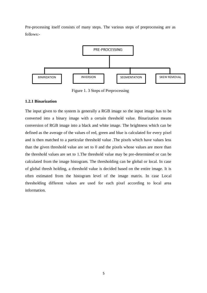
Pre-processing itself consists of many steps. The various steps of preprocessing are as
follows:-
Figure 1. 3 Steps of Preprocessing
1.2.1 Binarization
The input given to the system is generally a RGB image so the input image has to be
converted into a binary image with a certain threshold value. Binarization means
conversion of RGB image into a black and white image. The brightness which can be
defined as the average of the values of red, green and blue is calculated for every pixel
and is then matched to a particular threshold value .The pixels which have values less
than the given threshold value are set to 0 and the pixels whose values are more than
the threshold values are set to 1.The threshold value may be pre-determined or can be
calculated from the image histogram. The thresholding can be global or local. In case
of global thresh holding, a threshold value is decided based on the entire image. It is
often estimated from the histogram level of the image matrix. In case Local
thresholding different values are used for each pixel according to local area
information.

6
Figure 1. 4 Conversion from RGB Image to GRAY Image, GRAY Image to Binary image
1.2.2 Inversion
The process of conversion of white pixel to black and black pixel to white is known as
inversion. After binarization the image consists of black pixels in white background.
As we know white pixels have value binary 1 and the dark pixels have the value binary
0. So the numbers of pixels which are having value 1 are more than the number of
pixels which are having value 0. As all the methods are applied on pixel 1 so inversion
of the image is must so that the calculation can be lessened and hence we can make the
process fast and competent.
1.2.3 Skeletonization
Skeleton of a shape is a thin version of that shape i.e. equidistant from the boundaries.
We can also say that skeletonization is a conversion of a component of a digital image
into a subset of the original image. The pixels are removed in such a way that the

7
connectivity of original image is preserved. It is useful because it provides a simple
and compact representation of the shape of the image. There are various methods of
skeletonization which are as follows:-
1. The first category is based on distance transforms, where a definite subset of
the transformed image is distance skeleton. The original image can be restored
from the obtained distance skeleton.
2. The second category is based on thinning approach where the output of
skeletonization is a set of arcs and curves. The thinning can be achieved by
using the hit and miss transform method. The thinning is done with the help of a
structuring element .The origin of the structuring element is translated to each
and every position of the image. At every position the underlying pixels of the
image are compared to the structuring element .If the background and
foreground pixels of the image exactly matches that of the structuring element
then those pixels are set to 0 otherwise they are left unchanged.
1.2.4 Image segmentation
The process of portioning the image into its principle regions is called segmentation.
Segmentation is done to make the analysis easier. It is generally used to detect point,
line, edge, curves etc. Since the input to OCR system is generally handwritten text so
we have to separate each and every character exclusively [5]. So we can say that it is
one of the important steps of pre-processing.
Image segmentation can be further sub divided into:-
1. Implicit Segmentation, here words are predicted directly without segmenting the
word as individual letters.
2. Explicit Segmentation, here the word is segmented into individual character.
The segmentation can be done by many methods some of them are:-
a) Threshold based segmentation:- Here thresholding of histogram and slicing
technique is used for segmenting the image. This method can be applied directly
to the image.
b) Edge based segmentation:- In this method the edges of the image detected are
assumed to be the object boundaries which are used for identification.
c) Region based segmentation:- a region based technique initiates in the middle of
an object and then moving outward until and unless it encounters the object
8
boundaries.
d) Clustering techniques:- Clustering can be said as a synonym for segmentation
technique. Clustering method tries to group all pattern together which are similar in
some sense. This method is used for data analysis of high dimensional measurement
patterns.
e) Matching:- Matching approach is used when we know how the object looks like
which we wish to identify in an image.
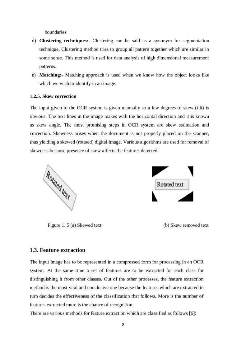
1.2.5. Skew correction
The input given to the OCR system is given manually so a few degrees of skew (tilt) is
obvious. The text lines in the image makes with the horizontal direction and it is known
as skew angle. The most promising steps in OCR system are skew estimation and
correction. Skewness arises when the document is not properly placed on the scanner,
thus yielding a skewed (rotated) digital image. Various algorithms are used for removal of
skewness because presence of skew affects the features detected.
Figure 1. 5 (a) Skewed text (b) Skew removed text
1.3. Feature extraction
The input image has to be represented in a compressed form for processing in an OCR
system. At the same time a set of features are to be extracted for each class for
distinguishing it from other classes. Out of the other processes, the feature extraction
method is the most vital and conclusive one because the features which are extracted in
turn decides the effectiveness of the classification that follows. More is the number of
features extracted more is the chance of recognition.
There are various methods for feature extraction which are classified as follows [6]:

9
1. Global Transformation and Series Expansion: includes Fourier Transform,
Gabor Transforms, Wavelets, moments and Karhuen-Loeve Expansion.
2. Statistical Method: In this method the features extracted from each and every
single character is combined which forms the feature vector for a particular
image. The various statistical method s are Zoning, Crossing and Distances,
Projections etc.
3. Geometrical and Topological Representation: Extracting and Counting
Topological Structures, Geometrical Properties, Coding, Graphs and Trees etc.
1.4. Classification
Here classifiers are used whose main purpose is to map features of the training set to a
group of feature vector of the training set. There are various approaches which can be
used for the process of classification and the approach varies depending on several real
world snags. Sometimes to get better efficiency a combination of different algorithms
can be used for the process of recognition which is more operative than using a single
character.
There are many various methods by which image can be classified. Given below are
some of the method which are generally used for the purpose of recognition. Every
classifier has his own advantages and disadvantages. The choice of classifier depends
on our purpose of use.
(a) HIDDEN MARKOVS MODEL
Here the system is trained with some hidden states and the output which we get is
dependent on the state and is visible. These type of models are generally used for
character recognition, speech recognition and gesture recognition [7]. In hidden
markovs model, the state is not directly visible, but output dependent on the state is
visible. This model can also be used where the observations are occurred due to some
probability distribution for example Gaussian distribution, in such a HMM the states
output is signified by a Gaussian distribution. The combination of two or more
Gaussians represents more complex behavior.

10
(b) SUPPORT VECTOR MACHINE
Support vector machines (SVMs,) are controlled learning models with related learning
algorithms that is used for evaluating data and for pattern recognition. An SVM model
is a depiction of the samples as points in space, mapped so that the samples of the
distinct types are separated by a clear gap that is as wide as possible. New samples are
then mapped into that same space and forecast to belong to a category based on which
side of the gap they fall on. Apart from performing linear classification, SVMs can
competently perform a classification which is non- linear using what is known as
kernel trick [8]. SVMs can be used in the following cases:
SVMs are useful for text and hypertext classification as their application can
meaningfully lessen the need for labeled training cases in standard inductive and as
well as transductive settings.
i. SVMs are used in cases where organization of images has to be performed.
Experimental results prove that SVMs attain considerably higher search
accuracy than customary query refinement systems after giving some
considerable amount of feedback.
ii. SVMs are also used in the field of medical science for the purpose of
classification.
iii. SVMs are also used for pattern recognition.
As everything as his own pros and cons similarly the disadvantages of support vector
machines are:
i. The accuracy decreases if the numbers of features are more than the number of
samples.
ii. They do not directly provide probability estimation, they are calculated using
an expensive five-fold cross-validation.
(c) ARTIFICIAL NEURAL NETWORK
Artificial neural networks (ANNs) motivated by an animal’s central nervous systems
which has the capability of machine learning and pattern recognition. . It resembles the
brain because of its capability to adapt learning process and the knowledge can also be
stored in synaptic weights which are the interconnections of neurons. ANNs are
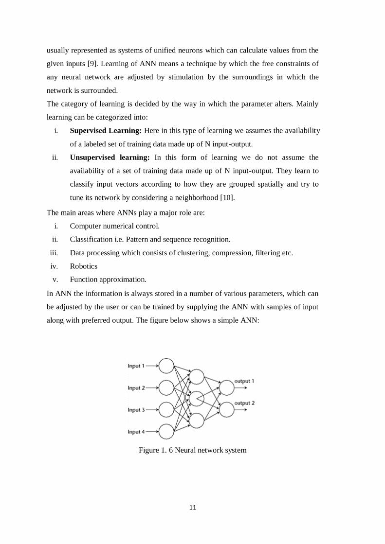
11
usually represented as systems of unified neurons which can calculate values from the
given inputs [9]. Learning of ANN means a technique by which the free constraints of
any neural network are adjusted by stimulation by the surroundings in which the
network is surrounded.
The category of learning is decided by the way in which the parameter alters. Mainly
learning can be categorized into:
i. Supervised Learning: Here in this type of learning we assumes the availability
of a labeled set of training data made up of N input-output.
ii. Unsupervised learning: In this form of learning we do not assume the
availability of a set of training data made up of N input-output. They learn to
classify input vectors according to how they are grouped spatially and try to
tune its network by considering a neighborhood [10].
The main areas where ANNs play a major role are:
i. Computer numerical control.
ii. Classification i.e. Pattern and sequence recognition.
iii. Data processing which consists of clustering, compression, filtering etc.
iv. Robotics
v. Function approximation.
In ANN the information is always stored in a number of various parameters, which can
be adjusted by the user or can be trained by supplying the ANN with samples of input
along with preferred output. The figure below shows a simple ANN:
Figure 1. 6 Neural network system

12
Types of Neural Networks
1. Multi-Layer Feed-forward Neural Networks.
Feed-forward ANNs transmits signals in one way only i.e. from input to output.
Feedback system is not available in such type of networks or we can say that the output
is independent. A feed-forward network appears to be straight forward networks that
associate inputs with outputs. These type of networks are widely used for pattern
recognition.
Figure 1. 7 Three layered neural network
In a three-layer network, the first layer known as input layer connects the input variables.
The last layer which is known as output layer. The layers present in between the input layer
and output layer are known as the hidden layer. In an ANN we can use more than one hidden
layer.
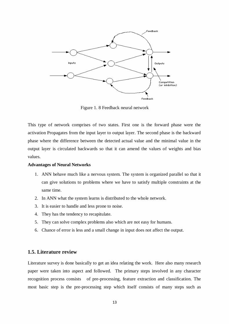
2. Multi-Layer Feed-back Neural Networks.
In a feedback networks the signals can travel directionally by using loops in the network.
Feedback networks are a bit complicated and at the same time very dominant. Feedback
networks are dynamic i.e. their state changes constantly till they reach a stability point. They
remain at the Stable point till the input changes and a new stability needs to be found.
Feedback neural network are also known to be communicative or persistent, even though the
last term is often used to represent feedback connections in single-layer organizations.
13
Figure 1. 8 Feedback neural network
This type of network comprises of two states. First one is the forward phase were the
activation Propagates from the input layer to output layer. The second phase is the backward
phase where the difference between the detected actual value and the minimal value in the
output layer is circulated backwards so that it can amend the values of weights and bias
values.
Advantages of Neural Networks
1. ANN behave much like a nervous system. The system is organized parallel so that it
can give solutions to problems where we have to satisfy multiple constraints at the
same time.
2. In ANN what the system learns is distributed to the whole network.
3. It is easier to handle and less prone to noise.
4. They has the tendency to recapitulate.
5. They can solve complex problems also which are not easy for humans.
6. Chance of error is less and a small change in input does not affect the output.
1.5. Literature review
Literature survey is done basically to get an idea relating the work. Here also many research
paper were taken into aspect and followed. The primary steps involved in any character
recognition process consists of pre-processing, feature extraction and classification. The
most basic step is the pre-processing step which itself consists of many steps such as

14
Binarization, Inversion, thinning, segmentation, noise reduction. A brief idea was also taken
on the difference between on-line and off-line character recognition processes various
research papers pertaining to feature extraction processes were gone through. The features
are essential for efficient recognition process. The better the features extracted the better will
be the result. There are many processes for this process but we have to choose our method
properly based on our input character. Then comes the process of classification and for the
same we use classifiers. Classifiers only give our final output. There are many types of
classifiers which were studied amongst them were hidden Markov model (HMM) and
artificial neural network (ANN).
1.6. Motivation
OCR is the most important process for humans and machine interface. A lot of research is
going on this area. Now a days OCR is very essential as slowly and steadily the world is
becoming automated and OCR helps in reducing human work load. A lot of research has
been done on English language but Devanagari which is used by a large number of
population in our country lags behind in the context of research. Various techniques were
studied and the best one was implemented on Devanagari text.
1.7. Organization of the thesis
The remaining of the thesis is organized as follows
Chapter 2 describes about the process of pre-processing.
Chapter 3 deals with the methods of feature extraction. Various methods of feature extraction
are described and the used method is explained.
Chapter 4 describes about the various methods of classification and the method used.
Chapter 5 thesis is concluded with the results and suggestions for future work.

15
CHAPTER 2
PRE-PROCESSING

16
PRE-PROCESSING
2.1 MORPHOLOGICAL OPERATIONS
Based on the shape of the image numerous image processing techniques are there for
processing images. The output of the morphological operation is of same size as input image
and it uses structuring element for the operation. In a morphological operation, comparison of
the corresponding pixel in the input image is done with its neighbors so as to get the value of
each pixel in the output image. For particular shapes in an input image, the morphological
operation can be constructed by varying the size and shape of the neighborhood [11].
There were various morphological operations which were performed on the input data which
are described below [12]:-
2.1.1. Erosion- It is the process of removing pixels on the object boundaries. The shape
of the structuring element used determines the number of pixels removed. The
process follows a particular rule according to which the value of the output pixel
is the least value of all the pixels in the input pixel’s neighborhood. If in a binary
image any of the pixel is set to 0, the output pixel is also set to 0.
The matlab function imerode is used for eroding an image.
2.1.2. Dilation- In this process pixels are added to the boundary of the objects in an
image. Here also structuring element decides the number of pixels to be added.
This process also follows a particular rule according to which the value of all the
pixels in the input pixel’s neighborhood is taken as the value of the output pixel.
For ex. If any of the pixel is set to the value 1, then the output pixel value is also
set to be 1.
The matlab function imdilate is used for dilation of the image.
2.1.3. Opening- The object contour is smoothened in this process by eradication of
portions and breaking of narrow strips. It uses the same structuring element as in
previous methods and the result of this operation is same as the combination of
erosion followed by dilation.
If image is denoted by set A and B is structuring element then operation is
denoted as follows
𝐴°𝐵 = (𝐴⊝ 𝐵)⊕ 𝐵
The above expression shows that the opening is result of erosion and followed
dilation of the erosion result by structuring element.
2.1.4. Closing- Closing is also used for soothing of the contours but opposite to that of

17
opening. It soothes the image by eradication of small holes and connection of
narrow breaks and filling of the gaps. It uses the same structuring element as in
previous methods and the result of this operation is same as the combination of
dilation followed by erosion.
If image is denoted by set A and B is structuring element then operation is
denoted as follows
A⋅B= = (𝐴⊕𝐵)⊖ 𝐵
The above expression shows that the closing is result of dilation and followed
erosion of the erosion result by structuring element.
Intensity transformations are applied to enhance the quality of the image for further
processing. The following transformations are applied on the colour JPEG image:
1. Conversion of RGB image into a Gray-scale Intensity image.
2. Conversion of Intensity image into a Binary image.
3. Inversion of the Binary image.
2.2 CONVERSION OF RGB IMAGE INTO A GRAY-SCALE
INTENSITY IMAGE
The above conversion can be performed by using the built-in MATLAB functions. The
image that is given as an input to the system can be an RGB colour image or a Grayscale
Intensity image. The algorithm has to checks whether the image is RGB image or not and if it
is an RGB image it converts it into a grayscale image, because all the further processing is
done in Grayscale format. Grayscale is preferred because of its ease in processing and for its
two dimensional matrix nature, and also it contains enough information needed for the actual
recognition.
The conversion is performed by using the MATLAB function rgb2gray.
2.3 CONVERSION OF GRAYSCALE IMAGE INTO A BINARY IMAGE
This conversion, also known as Image Quantization, produces a binary image from the
grayscale image by comparing pixel intensities with a threshold. This stage is very critical for
the car image. The threshold for Binarization can be two types static or dynamic. In static
general threshold is taken 150 (in gray scale of 0-255). This value reasonably quantizes those
pixels, which represents the license plate and any other portions, which has a pixel-value
more than the selected threshold. The remaining portions, which have a pixel-value less than

18
the threshold value, are darkened, as shown in Figure 3.2. In dynamic threshold, the
threshold taken will be the average of low and median gray scale values.
The conversion is done by using the MATLAB function im2bw.
2.4 INVERSION OF THE BINARY IMAGE
The process of conversion of white pixel to black and black pixel to white is known as
inversion. After binarization the image consists of black pixels in white background. As we
know white pixels have value binary 1 and the dark pixels have the value binary 0. So the
number of pixels which are having value 1 are more than the number of pixels which are
having value 0. As all the methods are applied on pixel 1 so inversion of the image is must so
that the calculation can be lessened and hence we can make the process fast and competent.
Inversion can be done by using negation in Matlab.
Other processes in preprocessing is
1. Labeling connected components in 2-D binary image.
2. Region props were used for measuring the properties of image. There are various
properties which can be measured. In our case Bounding Box and Area was
measured.
Bounding Box- This is smallest rectangle that an image can fit in to it.
Area- It specifies the actual number of pixels in the region.
3. Pixel list- It specifies the locations of pixels in the region.
4. Centroid- It specifies the center of mass of the region. The first element is the
horizontal coordinate (or x-coordinate), and the second is the vertical coordinate (or
y-coordinate).
Region props can be calculated by using Matlab functions.
5. The boundaries of the binary image were traced using bwboundaries function.
B = bwboundaries (BW, conn, options) postulates an optional argument, where
options can take any of the following values:
holes – It is used for finding out the both boundaries of object and hole.
noholes – It is used for finding boundary of object (parent and child) only.
This gives better performance.
While tracing the boundaries of parent and child Conn postulates the use of
connectivity. Conn can have either 4-connected neighborhood or 8-connected
neighborhood

19
6. The image was cropped using the imcrop function.
7. The image was then resized using the imresize command.
For ex. B=imresize (A, scale) after this operation we get an image B that is scale
times the size of A.
8. The image regions and holes were filled using the imfill function.
BW2 = imfill (BW, 'holes')
Here BW is a binary image containing holes which are filled by the MATLAB code
imfill.
9. Conversion of image to 8-bit unsigned integers.
I = im2uint8 (BW), im2uint8 takes an image as input and returns an image of class
uint8.
10. Bridges unconnected pixels, that is, sets 0-valued pixels to 1 if they have two nonzero
neighbors that are not connected. For example:
1 0 0 1 1 0
1 0 1 becomes 1 1 1
0 0 1 0 1 1
11. Thicken- This is morphological operation in which pixels are added to the exterior of
the objects for the purpose of thickening of objects. After this operation the
unconnected objects are results to 8-connected. This operation preserves the Euler
number.
2.5 Experimental results and discussion
The input image after going through various morphological operations and other
preprocessing steps gets ready for feature extraction. The results after performing the various
morphological operations is shown

20
Figure 2. 1 (a) Binary image (b) Inverted image (c) Filled image
Figure 2. 2 Images after basic morphological operations
.

21
CHAPTER 3
FEATURE EXTRACTION
22
3.1 Feature extraction
Features are essential for efficient recognition process. The better the features extracted the
better will be the result. There are many processes for this process but we have to choose our
method properly based on our input character. Features are generally categorized into two
different types, which are structural features such as strokes and bays, end points,
intersections of line segments loops and stroke relations, and other is the statistical features
which are derived from the statistical distribution of points. Statistical features comprises of
zoning, moments, n-tuples, characteristic loci [13]. The two features are opposite to each
other as both the features give different characters. To get the better results and to improve
the efficiency combination of both the approaches is used for feature extraction.
The extracted features should have the following properties:
1. Identifiability: The shapes which appear exactly similar to the human vision have the
identical features that are dissimilar from other feature.
2. Translation, rotation and scale invariance: The obtained feature must be invariant to
the change in location, rotation and scaling.
3. Affine invariance: the affine transformation is used for performing linear mapping
from one coordinates system to another coordinates system that conserves the
"straightness “and "parallelism" of lines. Affine transform is done by using various
processes of translations, scales, flips, rotations and shears. So the extracted features
must not be affected with affine transforms.
4. Noise hostility: The extracted features must be less affected by noise i.e., they must
not change if there is some noise or the strength of noise changes.
5. Occultation invariance: when some parts of an object gets obstructed by other objects,
the features extracted of the remaining part of the image must not differ.
6. Statistically independent: The different features extracted must not be statistically
dependent on each other.
7. Consistency: The extracted feature must be consistent i.e., the extracted features must
remain the same as long as we are dealing with the same pattern.
In our case we have used the shape based and contour features, the details of shape based
feature is explained below.

23
3.2 Shape based
Shape feature extraction methods are generally divided into two groups, they are contour
based methods and region based methods. The contour based method computes the shape
features only from the boundary of the shape, while the region based method extracts features
from the whole region.
Figure 3. 1 various methods for shape based feature extraction
Out of the various shape based feature the one based on theory of Moment was studied and
used in our project.
3.3 Theory of moments
The theory of moments was developed from the idea of moments in mechanics where mass
repartitions of objects are observed. Moments play a very important role for feature
extraction. The extracted features consists of shape area, the centre of the mass, the moment
of inertia which are known as the global properties of an image. Moments are basically of
two types orthogonal and non- orthogonal. Geometric moments were the primitive type of
24
moment which was used for the process of recognition [14, 15]. But due to the non
orthogonality property of the geometric moments reformation of the image from the features
is very complicated. The interpretation of accuracy of such moments is also not possible. The
most vital assets of the moments is their invariance under affine transformation [16, 17, 18]
Moments such as Tchebichef, Krawtchouk, dual Hahn, Racah and Hahn moments was used
for image analysis because of their better image representation ability than the continuous
orthogonal moments
3.3.1 Types of moments:
Moments are basically classified into two types which are further subdivided into other types.
The different types of moments are given below
I. Non-orthogonal Moments
In general the two-dimensional (2D) moment is given by
2
,.......2,1,0,,),(),(R
nmnm mndxdyyxfyx
Where,
f(x, y) is image intensity function and
ϕnm(x, y) is moment weighing kernel
By varying the basis functions, ϕnm , various moments can be found.
II. Orthogonal Moments (OM)
Two functions or vectors are said to be orthogonal if their inner product i.e. sum of
the product of their corresponding elements is zero. The geometric moment has the
projection of f(x, y) onto the monomials xnym. Unluckily, the basis set {xnym} is not
orthogonal. As a result, these moments are not ideal with respect to the information
retrieve capability. Apart from that the absence of orthogonally makes the recovery of
an image from its geometric moments difficult. To overcome the deficiencies related
with geometric moments, orthogonal moments came into existence [19]. Orthogonal
moments are robust to image noise. Orthogonal moments are further sub divided into
two types:-
A. Continuous orthogonal moments
These moments can be defined as continuous integrals over a domain of normalized
coordinates. The use of continuous orthogonal moment comprises the following
errors:
I. The discrete approximation of the continuous integrals
25
II. change of coordinate system of the image into the domain of the orthogonal
polynomials.
III. Analytical properties that the moment functions are supposed to fulfil such as
orthogonally and invariance are affected by the discrete approximation of
integrals. So to eliminate the above said problems discrete orthogonal moment
came into existence
B. Discrete orthogonal moments
To overcome one of the main problem associated with continuous orthogonal
moment i.e. the discretization error, which amasses with the increase in the order of
the moments discrete orthogonal moment came into existence [20]. The accuracy of
the calculated moments are thus affected. To overcome this problem, discrete
orthogonal moments came into existence. There are various discrete orthogonal
moments and tchebichef moment is one of them which was studied and used in our
case.
a. Tchebichef moments (TM)
For an image f(x, y) with size N×N, the Tchebichef moments of (n+m)th order is
defined as [21]
1
0
1 ~~
~~),,()()(
),().,(
1 N
x
N
oy
mnnm yxfytxt
NmNn
T
(14)
After going through all the various moment based methods, we have found that the
Tchebichef moment was best suitable for character recognition. Tchebichef moment
is explained in detail below.
The 2-D Tchebichef moment of order (n+m) of an image intensity function f(x, y)
with N x N is defined as
1
0
1
0
),()()(N
x
N
y
mnnm yxfytxtT
(1)
Here tn(x) is the nth order orthonormal Tchebichef polynomial and is defined as
.1,......,1,0,
)1()!(
)1()()(.
),(
)1()(
02
Nxn
Nk
nxn
Nn
Nxt
n
k k
kkkn
n
(2)
(a)k represents Pochhammer symbol

26
1)(1
)1)......(2)(1()(
0
aandk
Kaaaaa k
(3)
And the squared-norm (n,N) is given by
)!1)(12(
)!(),(
nNn
nNNn
(4)
Equation (2) can also be written as
n
k
kknn xcxt0
, )()(
(5)
Where
)!1(
)!1(.
)!()!(
)!(.
),(
)1(
)1(
)1(.
)!()!(
)!(.
),(
)1(
2
2,
nN
kN
kkn
kn
Nn
N
N
kkn
kn
Nnc
n
k
nk
kn
(6)
The orthogonally property leads to the following inverse moment transform
1
0
1
0
).()(),(N
n
N
m
mnnm ytxtTyxf
(7)
If only the moments of order up to (M-1, M-1) are computed,(7) is approximated by
1
0
1
0
~
).().(),(M
n
M
m
mnnm ytxtTyxf (8)
It has been shown that the reconstruction accuracy improves significantly by renormalization
of orthonormal Tchebichef moments [22]. We use this renormalized version of orthonormal
Tchebichef moments in our method.
3.4. Summary
Tchebichef moments are proved to have better image representation capabilities than
Legendre and Zernike moments and therefore can effectively be used in image analysis
applications including character recognition. In character recognition problem like in many
other pattern recognition problems, it becomes necessary to distinguish very similar
characters. At the same time, it is also necessary to identify different images of the same

27
character having some variations due to many factors like noise, font, size etc. as the images
of the same character. It is found in our study that, in spite of their superior image
representation capabilities, Tchebichef moments fail to distinguish characters which are very
similar in their shapes.
It has been observed in character recognition problems and also in other pattern recognition
problems that, in many cases, the distinguishing features are located in small parts of a group
of similar characters while the other parts are indistinguishable. These smaller parts
containing the distinguishing features can be discriminated with lower order moments in
comparison to the order of moments needed for the complete images. We have explored this
observation in the recognition of printed characters of the Devanagari numerals and found
that considerable improvement can be achieved in the recognition of characters through the
proposed method. By using tchebichef moments, the problems associated to continuous
orthogonal moments are eliminated by using a discrete orthogonal basis function. Apart from
that mapping is also not required to compute Tchebichef moments due to the orthogonality
property of the Tchebichef polynomials.
3.4.1. Limitations of moment-based character recognition methods
Theoretically, the representation accuracy should increase with the order of moments used to
represent the characters. But, the computational requirement also increases with the number
of moments. It is also evidenced from experiments that effectiveness of the representation
space does not improve beyond a certain level even when the size of the moment vector is
increased. It may be mentioned here that the effectiveness of a representation space is
determined by how well patterns from different classes can be separated [23].
The second approach for feature extraction was based on the contour.
3.5 Contour based method
This was the second method used for the process of feature extraction which is explained
below.
Shape based methods can be broadly divided into two class of methods:
Contour based methods and region-based methods. The classification is dependent on
whether shape features are extracted from the contour only or are extracted from the whole
shape region. Under each class, the various methods are further divided into structural
approaches i.e. the shape is represented by segments and global approaches where the shape
28
can be represented as a whole. These approaches can be further divided into space domain
and transform domain.
Contour shape methods only find the shape boundary information. There are generally two
types of approaches for contour detection first one is the continuous approach or global
approach and second one is the discrete approach or the structural approach. In continuous
approach shape is not divided into sub-parts, usually a feature vector derived from the
integral boundary is used to describe the shape. The measure of shape similarity is usually a
metric distance between the attained feature vectors. In discrete approaches the shape
boundary is broken down into segments, called primitives using a particular criterion [24].
Shape feature extraction is used in the following applications:
Shape recovery
Classification and shape recognition
Registration and shape alignment
Simplification and shape approximation
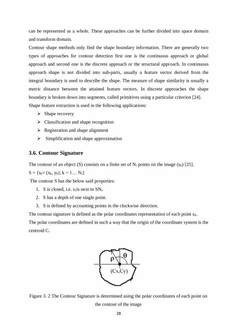
3.6. Contour Signature
The contour of an object (S) consists on a finite set of Ni points on the image (sk) [25].
S = {sk= (xk, yk); k = 1… Ni}
The contour S has the below said properties:
1. S is closed, i.e. s1is next to SNi.
2. S has a depth of one single point.
3. S is defined by accounting points in the clockwise direction.
The contour signature is defined as the polar coordinates representation of each point sk.
The polar coordinates are defined in such a way that the origin of the coordinate system is the
centroid C.
Figure 3. 2 The Contour Signature is determined using the polar coordinates of each point on
the contour of the image

29
In contour signature the centroid is calculated and the distance between centroid and
boundary points is calculated. After that the angle which the boundary point made to the
centroid is also determined according to the formula as described below. As the number of
boundary points are different for each image so an algorithm was applied to make the number
of boundary points same.
1. We have selected sample value of boundary point as the average value of the
maximum and minimum value of boundary points.
i. NNN= (max.+min.)/2
2. Let the number of boundary points of an arbitrary image is Ni. Then the algorithm
will convert all boundary points to NNN as shown in the algorithm.
If (NNN)> Ni
Then ceil i.e. round towards positive infinity
Else
Round i.e. round to nearest integer
3.6.1. Centroid
The centroid also known as centre of gravity. Its position is fixed in relation to the shape.
Suppose that shape is represented by its region function, then centroid (gx, gy) is given by:
Where N is the number of point in the shape,
The general function f(x,y) is :
Dyxif
otherwiseyxf ),(1
0),(
Where D is the domain of the binary shape.

30
Figure 3. 3 Centroid of the image.
3.6.2. Tangent Angle
The tangent angle function at a point Pn(x(n), y(n)) is given by a tangential direction of a
contour at that point [26]:
wnxnx
wnynyn n
arctan
w is a small window to calculate θ (n)
Tangent angle has its own snags which are as follows:
1) Noise sensitivity- To reduce the effect of noise, we use a low-pass filter with suitable
bandwidth before determining the tangent angle function.
2) Discontinuity- The tangent angle function value is assumed in the range of length 2π,
usually in the interval of [-π, π] or [0, 2π]. So θn in general contains discontinuities of
size 2π. To reduce the problem of discontinuity, the cumulative angular function φn is
known as the angle differences between the tangent at any point Pn along the curve and
the tangent at the starting point P0.
3.7. Experimental results and discussions
Both the above methods of feature extraction was implemented on both the training data set
as well as testing data set. Our training data consists of 2000 images whereas the testing data
consists of 500 images. The feature set extracted for training data set by using the Tchebichef

31
moment consists of a matrix of size 81 x 2000 i.e. we can say that a total of 81 features were
extracted for each single. Similarly 81x 500 for the testing data.
In case of contour signature we got a matrix of size 412 x 2000 for training data set and 412 x
500 for testing data set. Out of the 412 feature extracted 206 features gives the distance
between centroid and boundary points and the remaining 206 features gives the angle.
After going through the various methods of feature extraction I assumed there must be some
hidden attributes which were undetected by both the methods and hence to overcome this
problem I opted for feature cascading which is nothing but addition of both the features
obtained. The resultant feature vector was given to the classifier. Suppose there are x and y
different feature vectors therefore their resultant feature after feature cascading will be (x+y)
.In our case the resultant feature vector size was 493 x 2000.

32
CHAPTER 4
CLASSIFICATION
33
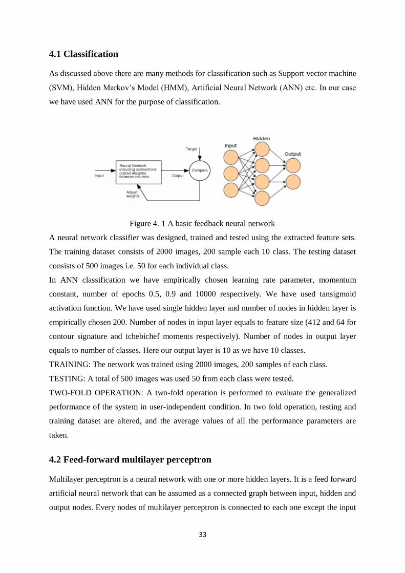
4.1 Classification
As discussed above there are many methods for classification such as Support vector machine
(SVM), Hidden Markov’s Model (HMM), Artificial Neural Network (ANN) etc. In our case
we have used ANN for the purpose of classification.
Figure 4. 1 A basic feedback neural network
A neural network classifier was designed, trained and tested using the extracted feature sets.
The training dataset consists of 2000 images, 200 sample each 10 class. The testing dataset
consists of 500 images i.e. 50 for each individual class.
In ANN classification we have empirically chosen learning rate parameter, momentum
constant, number of epochs 0.5, 0.9 and 10000 respectively. We have used tansigmoid
activation function. We have used single hidden layer and number of nodes in hidden layer is
empirically chosen 200. Number of nodes in input layer equals to feature size (412 and 64 for
contour signature and tchebichef moments respectively). Number of nodes in output layer
equals to number of classes. Here our output layer is 10 as we have 10 classes.
TRAINING: The network was trained using 2000 images, 200 samples of each class.
TESTING: A total of 500 images was used 50 from each class were tested.
TWO-FOLD OPERATION: A two-fold operation is performed to evaluate the generalized
performance of the system in user-independent condition. In two fold operation, testing and
training dataset are altered, and the average values of all the performance parameters are
taken.
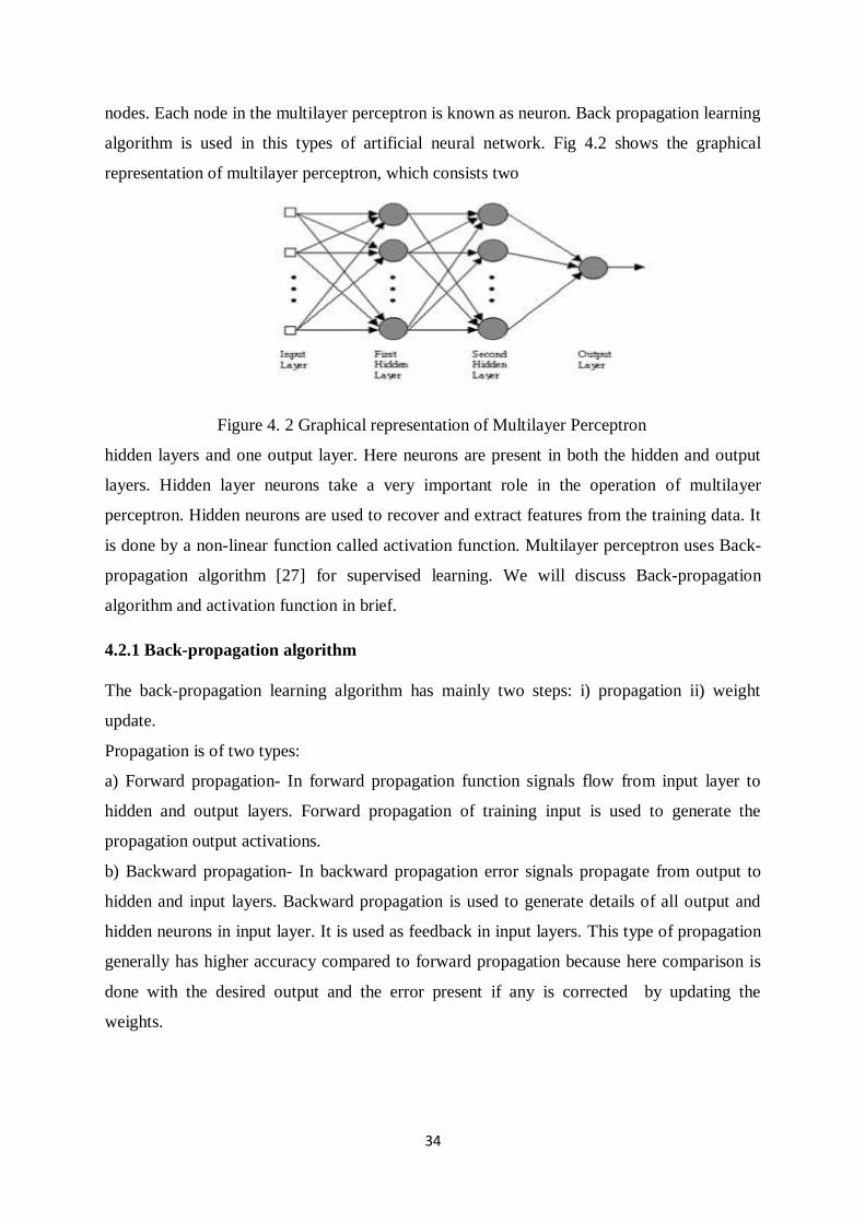
4.2 Feed-forward multilayer perceptron
Multilayer perceptron is a neural network with one or more hidden layers. It is a feed forward
artificial neural network that can be assumed as a connected graph between input, hidden and
output nodes. Every nodes of multilayer perceptron is connected to each one except the input
34
nodes. Each node in the multilayer perceptron is known as neuron. Back propagation learning
algorithm is used in this types of artificial neural network. Fig 4.2 shows the graphical
representation of multilayer perceptron, which consists two
Figure 4. 2 Graphical representation of Multilayer Perceptron
hidden layers and one output layer. Here neurons are present in both the hidden and output
layers. Hidden layer neurons take a very important role in the operation of multilayer
perceptron. Hidden neurons are used to recover and extract features from the training data. It
is done by a non-linear function called activation function. Multilayer perceptron uses Back-
propagation algorithm [27] for supervised learning. We will discuss Back-propagation
algorithm and activation function in brief.
4.2.1 Back-propagation algorithm
The back-propagation learning algorithm has mainly two steps: i) propagation ii) weight
update.
Propagation is of two types:
a) Forward propagation- In forward propagation function signals flow from input layer to
hidden and output layers. Forward propagation of training input is used to generate the
propagation output activations.
b) Backward propagation- In backward propagation error signals propagate from output to
hidden and input layers. Backward propagation is used to generate details of all output and
hidden neurons in input layer. It is used as feedback in input layers. This type of propagation
generally has higher accuracy compared to forward propagation because here comparison is
done with the desired output and the error present if any is corrected by updating the
weights.

35
Weight update is done by the following steps a) multiply local gradient and input signal of
neuron b) subtract a portion of the gradient from the weight. It can be expressed by the
following formula
( ) ( ) ( )Weight correction learning rate parameter local gradient input signal of neuron
4.2.2. Activation function
Hidden neurons are used to recover and extract features from the training data. It is done by a
non-linear function called activation function. Computation of local gradient is related to the
derivative of the activation function. For that purpose, activation function is very important in
Multi-layer perceptron. There are mainly two types of activation functions: a) Logistic
Function: b) Hyperbolic tangent function
Logistic function: This type of activation functions are expressed by the following equation
1( ( ))
1 exp( ( ))j j
j
v nav n
(4.1)
Where, vj(n) is the local field of neuron j and a is an adjustable positive parameter.
Differentiating equation (4.2) with respect to vj(n), we get
'
2
exp( ( ))( ( ))
[1 exp( ( ))]
j
j j
j
a av nv n
av n
(4.2)
Now from the activation function we can get local gradient as given by the following formula
'( ) ( ) ( ( ))j j j jn e n v n (4.3)
Hyperbolic tangent function:
This type of activation functions are expressed by the following equation
( ( )) tanh( ( ))j j jv n a bv n (4.4)
' 2( ( )) sec ( ( ))j j jv n ab h bv n (4.5)
Now from the activation function we can get local gradient as given by the following formula
'( ) ( ) ( ( ))j j j jn e n v n (4.6)

36
In our proposed Artificial Neural Network classifier we have used tan sigmoid activation
function.
In an ANN classifier the feature size depicts the number of input layer present in the network.
So in our case the number of input layers were 412 for contour signature and 81 for
tchibichef moment. We have empirically selected number of hidden neurons as 200.
4.3 Performance matrices
The classification performance was determined using accuracy, sensitivity, specificity and
positive predictivity. Overall accuracy (A) of the classifier is defined as
100 1 e
b
NA
N
In this equation A is the overall accuracy and the variable 𝑁𝑒 and 𝑁𝑏 represent the total
number of misclassified images and total number of images, respectively. Other parameters
which are computed are Accuracy (Ac), Sensitivity (Se), Specificity (Sp) and Positive
Predictivity (Pp). These parameters are given by the subsequent equations.
c
TP TNA
TP TN FP FN
e
TPS
TP FN
p
TNS
TN FP
p
TPP
TP FP
Where,
TP- True positive are those images which belong to a particular class and are correctly
allotted to that class only.
FP- False positive are those images which belongs to some other class incorrectly allotted to
that same class.
TN- True negative are those images which doesn’t belongs to a particular class and in the
output also it was correctly not allotted that class.

37
FN- False negative are those image which should have been assigned to a particular class but
was not allotted to that class and allotted to another class
Consequently, sensitivity shows how accurately a classifier recognizes images of a certain
class. Positive predictivity gives the true positive images in all the images. Specificity shows
the ability to reject correctly and accuracy gives the overall performance of the system.
4.4 Experimental results and discussions
The confusion matrix obtained from the classifier is shown below for both the features in
table4.1 and table 4.2 respectively
Class 0 1 2 3 4 5 6 7 8 9
0 47 0 0 0 1 0 0 2 0 0
1 0 40 4 0 0 0 0 0 0 6
2 2 3 44 0 0 0 0 0 0 1
3 1 0 0 28 10 2 7 0 0 2
4 0 0 0 0 33 12 0 3 0 2
5 0 0 0 5 13 30 0 0 2 0
6 0 0 0 0 1 0 48 0 1 0
7 1 0 0 0 0 0 0 49 0 0
8 2 5 0 0 0 0 0 11 32 0
9 0 2 0 0 0 0 0 0 12 36
Table 4. 1 Confusion matrix of Contour signature feature
From the above confusion matrix we can observe that maximum miss classification occurred
in case of 3 followed by 8, 4 and 9

38
Class 0 1 2 3 4 5 6 7 8 9
0 49 0 0 0 1 0 0 0 0 0
1 0 43 3 0 0 0 0 4 0 0
2 0 12 32 3 0 0 0 0 0 3
3 0 0 0 50 0 0 0 0 0 0
4 3 0 0 0 31 15 0 1 0 0
5 0 0 0 0 0 50 0 0 0 0
6 0 0 2 0 3 0 40 0 5 0
7 6 0 0 0 3 0 0 34 7 0
8 0 0 0 0 0 0 0 0 50 0
9 0 0 0 0 0 0 0 0 0 50
Table 4. 2 Confusion matrix of Tchebichef moment feature
From the above confusion matrix we can observe that miss classification occurred in case of
4 followed by 2 and 7.
The performance of the classifier was determined using the four parameters they are
accuracy, sensitivity, Specificity and positive predictivity. Performance of both the methods
is shown in table 4.3 and Fig.4.1. From the table we can observe that Tchebichef moment
gives better result compared to contour signature method moment in all respects.
Features Accuracy Sensitivity Positive
Predictivity
Specificity
Contour signature 95.48 77.4 77.76 97.48
Tchebichef moment 97.16 85.80 86.41 98.42
Table 4. 3 Performance comparison of various features

39
Figure 4. 3 Performance comparison of two features
From the table we can observe that classification accuracy of contour signature and
Tchebichef moment are 77.4% and 85.8% respectively, as shown in table4.3
To improve classification accuracy we used feature cascading as discussed in chapter 3. In
that case, we observe that classification performance has improved. In table below we can see
that the sensitivity has increased to 87.4% after cascading. Below we can see the confusion
matrix and other parameters.
Table 4. 4 Confusion matrix of contour -Tchebichef cascading feature
0
20
40
60
80
100
120
Accuracy Sensitivity pos.pred Specificity
Contour
Tchebichef
Class 0 1 2 3 4 5 6 7 8 9
0 49 0 0 0 1 0 0 0 0 49
1 0 42 5 0 0 0 0 0 0 0
2 0 8 38 4 0 0 0 0 0 0
3 0 0 0 44 0 0 6 0 0 0
4 3 0 0 0 35 14 0 1 0 3
5 0 0 0 0 0 50 0 0 0 0
6 0 0 0 0 2 0 47 0 1 0
7 5 0 0 0 0 0 0 43 2 5
8 5 0 0 0 0 0 0 3 42 5
9 0 1 0 0 0 0 0 0 0 49
40
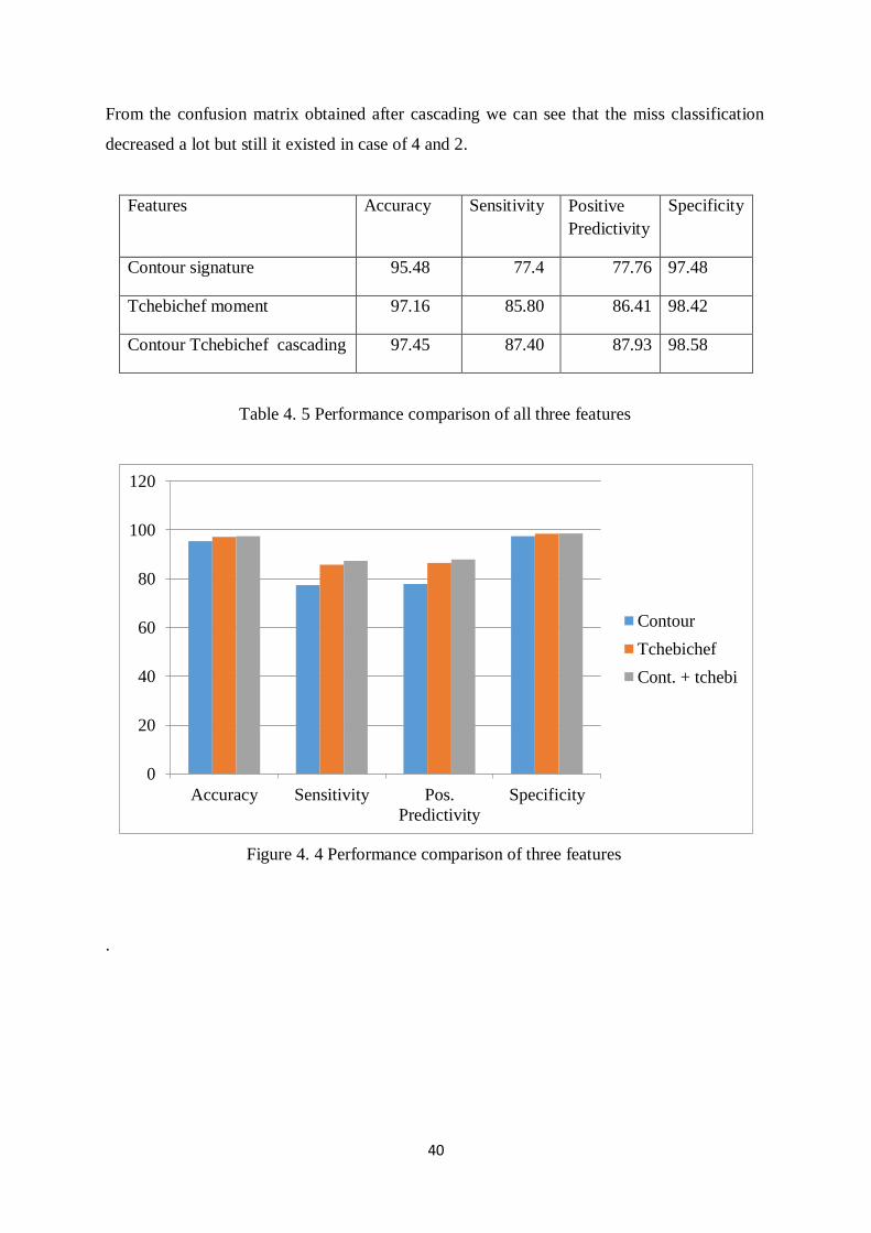
From the confusion matrix obtained after cascading we can see that the miss classification
decreased a lot but still it existed in case of 4 and 2.
Features Accuracy Sensitivity Positive
Predictivity
Specificity
Contour signature 95.48 77.4 77.76 97.48
Tchebichef moment 97.16 85.80 86.41 98.42
Contour Tchebichef cascading 97.45 87.40 87.93 98.58
Table 4. 5 Performance comparison of all three features
Figure 4. 4 Performance comparison of three features
.
0
20
40
60
80
100
120
Accuracy Sensitivity Pos.
Predictivity
Specificity
Contour
Tchebichef
Cont. + tchebi

41
CHAPTER 5
CONCLUSION AND FUTURE
WORK

42
5.1 CONCLUSION
OCR has been the area of interest from past many years. The motive of this project was to
develop an offline character recognition system. The motive was to recognize devnagari
numerals. Here we have used two types of features first one was contour based and second
one was moment based. Prior to that basic morphological operation were performed to make
the data fit for feature extraction. The work was completed by using an ANN classifier.
A total of 2000 images were taken for training the network and 500 images were taken for
testing. The performance was compared for both the features. The sensitivity was found to be
77.4% for contour based features and 85.80% for Tchebichef based features. I assumed that
there may be some hidden attributes which cannot be determined by using single type of
features, so I cascaded the features obtained by both the methods to get a feature set which
have some extra features. The cascaded features were used for testing and training and we
observed that the performance parameters increased significantly. The specificity increased to
87.40% from 85.80%. Here misclassification occurred in case of 1and 2, 4 and 5.
5.2 FUTURE WORK
The area of character recognition is very wide. Here we have recognized devnagari numerals.
Work can be done for recognition of devnagari alphabets and other regional languages
because regional language lags behind in the matter of research compared to other languages.
Here we have recognized offline characters work can also be done for online character
recognition.

43
REFERNCES
[1] V.K. Govindan and A.P. Shivaprasad, “Character Recognition – A review,” Pattern
Recognition, Vol. 23, no. 7, pp. 671- 683, 1990.
[2] Plamondon Rejean, Sargur N. Srihari, “On line and off line handwriting recognition:
A comprehensive survey”, IEEE Transactions on PAMI, vol. 22, No. 1, 2000.
[3] Anil K. Jain, Robert P. W. Duin, Jianchang Mao, “Statistical Pattern Recognition:A
Review”, IEEE Transactions on PAMI, Vol. 22, No. 1, pp. 4-37, January 2000.
[4] R. O. Duda, P. E. Hart, D. G. Stork, “Pattern Classification”, second ed., Wiley-
Interscience, New York 2001.
[5] R.G. Casey and E.Lecolinet, “A Survey of Methods and Strategies in Character
Segmentation,” IEEE Transactions on Pattern Analysis and Machine Intelligence,
Vol. 18, No.7, July 1996, pp. 690-706
[6] C.-L. Liu, K. Nakashima, H. Sako, andH. Fujisawa, “Handwritten digit recognition:
Bench-marking of state-of-the-art techniques”, Pattern Recognition. 36 (10), 2271–
2285, 2003.
[7] A. Rajavelu, M. T. Musavi, and M. V. Shirvaikar, “ANeural Network Approach to
Character Recognition,” Neural Networks, 2, pp. 387-393, 1989.
[8] J. X. Dong, A. Krzyzak, C. Y. Suen, “An improved handwritten Chinese character
recognition system using support vector machine”, Pattern Recognition Letters.
26(12), 1849–1856, 2005
[9] S.C.W. Ong, S. Ranganath, “Automatic sign language analysis: a survey and the
future beyond lexical meaning”, IEEE Transactions on Pattern Analysis and Machine
Intelligence 27 (6) (2005) 873–891.
[10] D. S. Zhang and G. Lu, “A comparative study on shape retrieval using fourier
descriptors with different shape signatures”, in Proc. International Conference on
Intelligent Multimedia and Distance Education (ICIMADE01), 2001
[11] Rafael C. Gonzalez, Richard E. woods and Steven L.Eddins, “Digital Image
Processing using MATLAB”, Pearson Education, Dorling Kindersley, South Asia,
2004.
[12] Y. Kimura, T. Wakahara, and A. Tomono, “Combination of statistical and neural
classifiers for a high-accuracy recognition of large character sets”, Transactions of
IEICE Japan. J83-D-II (10), 1986–1994, 2000 (in Japanese).

44
[13] S.C.W. Ong, S. Ranganath, “Automatic sign language analysis: a survey and the
future beyond lexical meaning”, IEEE Transactions on Pattern Analysis and Machine
Intelligence 27 (6) (2005) 873–891
[14] R. Mukundan, K.R. Ramakrishnan, “Moment Functions in Image Analysis: Theory
and Applications”, World Scientific Publishing Co.Pte.Ltd. 1998.
[15] D. Trier, A. K. Jain, T. Taxt, “Feature Extraction Method for Character Recognition -
A Survey”, Pattern recognition, vol. 29, no. 4, pp. 641-662, 1996.
[16] M. Mitchell, “An Introduction to Genetic Algorithms”, MIT Press, 1998.
[17] Hu, M.K., “Visual pattern recognition by moment invariants” IRE Transactions on
Information Theory 8, 179–187, 1962.
[18] Teague MR, “Image analysis via the general theory of moments”, J Opt SocAm.1980;
70:920–930.
[19] Yap PT, Paramesran R, Ong SH, “Image Analysis by Krawtchouk Moments”, IEEE
Trans Image Processing, 12:1367–1377, 2003. [PubMed]
[20] Mukundan R, Ong SH, Lee PA, “Image analysis by Tchebichef moments”, IEEE
Trans Image Process, 10:1357–1364, 2001. [PubMed]
[21] R. Mukundan, “Improving image reconstruction accuracy using discrete orthonormal
moments”, in Proc. Intnl. Conf. on Imaging Systems, Science and Technology
(CISST), pp. 287-293, 2003.
[22] A. K. Jain, R. P. W. Duin, and J. Mao, “Stastical pattern recognition: A review,”
IEEE PAMI, vol. 22, no. 1, pp. 5–37, Jan 2000.
[23] Yang Mingqiang, Kpalma Kidiyo and Ronsin Joseph, “A survey of shape feature
extraction techniques”, July 15, 2008.
[24] Paulo Peixoto, Paulo Peixoto, “A natural hand gesture human computer interface
using contour signatures”.
[25] Richard O. Duda, Peter E. Hart, and David E. Stork, “Pattern Classification”, Wiley,
New York, second edition, 2001.
[26] K.-J. Lu and S. Kota, “Compliant mechanism synthesis for shape-change applications:
Preliminary results”, in Proceedings of SPIE Modeling, Signal Processing, and
Control Conference, vol. 4693, March 2002, pp. 161-172.
[27] Y. Kimura, T. Wakahara, and A. Tomono, “Combination of statistical and neural
classifiers for a high-accuracy recognition of large character sets”, Transactions of
IEICE Japan, J83-D-II (10), 1986–1994, 2000 (in Japanese).