Electronic Supplementary Information Supplementary Information ... Naming convention of the video files: ... We have not measured the 3-phase contact angle of the drop at the PDMS

1

Break-up of droplets in a concentrated emulsion flowing through a narrow

constriction

Liat Rosenfeld, Lin Fan, Yunhan Chen, Ryan Swoboda, and Sindy K.Y. Tang*

Department of Mechanical Engineering, Stanford University, CA 94305

*Corresponding author: [email protected]

Electronic Supplementary Information

Electronic Supplementary Material (ESI) for Soft MatterThis journal is © The Royal Society of Chemistry 2013

2

Supplementary Note 1: Synthesis of surfactant ammonium salt of Krytox. We found that Krytox alone could not stabilize aqueous drops in HFE-7500 against coalescence. The ammonium salt of Krytox, on the other hand, generated much more stable drops. The synthesis steps of the latter are as follows. 1. Add 20 g of Krytox 157 FSL (DuPont) to 180 g methanol in a 500 ml Erlenmeyer flask

equipped with vigorous magnetic stirring. 2. Add, drop-wise, 28 % (wt.%) ammonium hydroxide solution (NH4OH(aq)) and stir

continuously. Total amount of NH4OH(aq) added was about 0.6 g. 3. Continue step 2 until the cloudy, two-phase mixture became clear, and when the pH becomes

pH 7. 4. Remove the solvent by rotary evaporation.

Supplementary Note 2: Estimation of strain rate in contraction region. We consider a fluid element with dimensions l being stretched dl as it enters the constriction. We ignore shear for now. Strain can be written as 휀 = . From geometry we know = , and

( )( )

= ( )( )

. So:

휀 =푑푙푙 =

2tan(훼)푑푥푤(푥)

Strain rate G can be found by taking the derivative of 휀 with respect to time:

퐺 =푑휀푑푡 =

푑푥푑푡

2tan(훼)푤(푥) =

2푣(푥)tan(훼)푤(푥)

Alternatively, according to the derivation of equation (1) from reference 1, we can estimate the overall strain rate G in the contraction area as the change in the average fluid velocity at the

entrance region (v0) and at the constriction (v) over the contraction length (푙 =( )

):

퐺~ ∆ ~ ~2 ( ) 푣tan(훼).

In either case, G ~ tan(). We thus expect the break-up dynamics to scale with tan(). Supplementary Videos Set 1: Single drops did not split in our system. Videos show that single droplets passing through the constriction did not split at the highest flow rates used in the reinjection experiments for channels with entrance angles of 5° and 30°


3

respectively. From these videos, we conclude that droplet splitting was primarily due to droplet-droplet interactions. Naming convention of the video files: total flow rate_entrance angle_drop volume_frame rate_SingleDropFlow.avi For example, “3p0mLhr_5degch_40pLdrops_41237fps_SingleDropFlow.avi” means the video is recorded for an experiment at a total flow rate of 3.0 mL/hr in a channel with 5 degrees of entrance angle for drops that have a volume of 40 pL. The video is recorded at 41,237 frames per second (fps) for the flow of single drops only. Supplementary Videos Set 2: Representative movies of reinjection of concentrated emulsions. Naming convention of the video files: total flow rate_entrance angle_drop volume_frame rate_number of frames.avi Supplementary Videos Set 3: Representative movies of droplet tracking at upstream/downstream locations and direct imaging at the constriction. Naming convention of the video files: total flow rate_entrance angle_drop volume_region of imaging.avi MATLAB code. MATLAB code for tracking droplets will be provided upon request.


4

Supplementary Figure S1: Calculation of the number of droplet break-up events

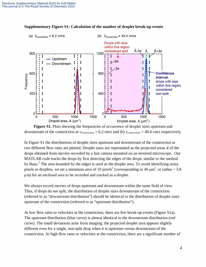
Figure S1. Plots showing the frequencies of occurrence of droplet sizes upstream and

downstream of the constriction at vconstriction = 6.2 cm/s and (b) vconstriction = 49.4 cm/s respectively. In Figure S1 the distributions of droplet sizes upstream and downstream of the constriction at two different flow rates are plotted. Droplet sizes are represented as the projected areas 퐴 of the drops obtained from movies recorded by a fast camera mounted on an inverted microscope. Our MATLAB code tracks the drops by first detecting the edges of the drops, similar to the method by Basu.2 The area bounded by the edges is used as the droplet area. To avoid identifying noisy pixels as droplets, we set a minimum area of 10 pixels2 (corresponding to 46 μm2, or radius ~ 3.8 m) for an enclosed area to be recorded and tracked as a droplet. We always record movies of drops upstream and downstream within the same field of view. Thus, if drops do not split, the distribution of droplet sizes downstream of the constriction (referred to as “downstream distribution”) should be identical to the distribution of droplet sizes upstream of the constriction (referred to as “upstream distribution”). At low flow rates or velocities at the constriction, there are few break-up events (Figure S1a). The upstream distribution (blue curve) is almost identical to the downstream distribution (red curve). The small deviations arise from imaging: the projected droplet area appears slightly different even for a single, non-split drop when it is upstream versus downstream of the constriction. At high flow rates or velocities at the constriction, there are a significant number of


5

break-up events (Figure S1b). Upstream distribution obviously deviates from downstream distribution. Quantification of the number of split drops from the distributions of droplet sizes upstream and downstream of the constriction. We first observe that upstream distribution is normal with a standard deviation, 휎 ~ 3.3%. We define a 3-standard deviation confidence interval to include 99.7% of the upstream droplets (corresponding to ~ 4985 drops out of 5000 drops) centered about the mean droplet size, 퐴̅. The upper and lower bounds of this interval are 퐴̅ + 3휎 and 퐴̅ − 3휎 respectively, as shown in Figure S1b. This confidence interval indicates the expected droplet sizes at the initial non-split state. If the drops do not split passing through the constriction, we expect the downstream distribution (red curve) to fall within this interval, as shown in Figure S1a. If the drops split, the number of drops with sizes smaller than 퐴̅will increase. We define the region outside of the confidence interval (shaded in pink in Figure S1b), specifically droplet size < 퐴̅ − 3휎, as indicative of break-up events. To account for parent drops with initial sizes outside of the confidence interval, we subtract the upstream distribution from the downstream distribution for all discussions below. The following discussion refers to Figure S1b. From video analysis, we know that for each break-up event, one upstream parent always splits into two downstream daughter droplets (for > 300 drops observed manually). If we assume all upstream droplets have an area equal to 퐴̅and area is conserved between upstream parent and downstream daughter droplets, we can see that two cases exist: (1) An upstream parent droplet splits into a large downstream daughter droplet with size within

{퐴̅ − 3휎, 퐴} , and a small downstream droplet with area less than 3휎. (2) An upstream parent droplet splits into two downstream droplets with areas within {3휎, 퐴̅ −

3휎}. For case (1), since we ignore the region within the confidence interval in our accounting for break-up events, we can only observe 1 downstream daughter droplet with size less than 3휎. Thus, in this case, the number of break-up events (or, the number of upstream drops that split) is equal to the number of downstream droplets with size less than 3휎. For case (2) we observe 2 downstream daughter droplets with areas within {3휎, 퐴̅ − 3휎} that were produced by 1 upstream parent droplet. Thus, in this case, the number of break-up events (or, the number of upstream drops that split) is equal to 1/2 of the number of downstream droplets with size within {3휎, 퐴̅ − 3휎}.


6

Estimation of errors in the quantification split drops. Our quantification method will have errors because not all parent drops upstream have a size exactly equal to the mean 퐴̅. There is variation in droplet size as shown by the confidence interval. We can estimate the upper limit of this error by assuming all droplets that split have a size of 퐴 = 퐴̅ + 3휎. In this scenario, the two cases will be:

(1) An upstream droplet splits into a large downstream droplet with size within {퐴̅ − 3휎, 퐴̅ + 3휎}, and a small downstream droplet with area less than 6휎.

(2) An upstream droplet splits into two downstream droplets with areas within {6휎, 퐴̅ − 3휎}. For case (1), since we ignore the region within the confidence interval in our accounting for break-up events, we only observe 1 downstream droplet with size less than 6휎 that was produced by 1 upstream droplet. Thus, in this case, the number of upstream droplets split is equal to the number of downstream droplets with size less than 6휎. For case (2) we observe 2 downstream droplets with areas between within {6휎, 퐴̅ − 3휎} that were produced by 1 upstream droplet. Thus, in this case, the number of upstream droplets split is equal to 1/2 of the number of downstream droplets with size within {6휎, 퐴̅ − 3휎}. We calculated the number of droplets that split based on the above discussion to obtain the upper limit of the error bars in Figures 2c and 2f in the main text. Similarly, we can estimate the lower limit of the error by assuming all droplets that split have size 퐴 = 퐴̅ − 3휎. In this scenario, there is only one case. Every upstream droplet that is split will split into two downstream droplets with size less than 퐴̅ − 3휎. Thus, in this case, the number of upstream droplets split is equal to 1/2 of the number of downstream droplets with size less than 퐴̅ − 3휎. We calculated the number of droplets that split based on the above discussion to obtain the lower limit of the error bars in Figures 2c and 2f in the main text.


7

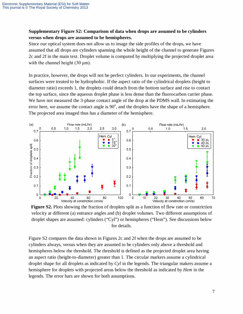
Supplementary Figure S2: Comparison of data when drops are assumed to be cylinders versus when drops are assumed to be hemispheres. Since our optical system does not allow us to image the side profiles of the drops, we have assumed that all drops are cylinders spanning the whole height of the channel to generate Figures 2c and 2f in the main text. Droplet volume is computed by multiplying the projected droplet area with the channel height (30 μm). In practice, however, the drops will not be perfect cylinders. In our experiments, the channel surfaces were treated to be hydrophobic. If the aspect ratio of the cylindrical droplets (height to diameter ratio) exceeds 1, the droplets could detach from the bottom surface and rise to contact the top surface, since the aqueous droplet phase is less dense than the fluorocarbon carrier phase. We have not measured the 3-phase contact angle of the drop at the PDMS wall. In estimating the error here, we assume the contact angle is 90o, and the droplets have the shape of a hemisphere. The projected area imaged thus has a diameter of the hemisphere.

Figure S2. Plots showing the fraction of droplets split as a function of flow rate or constriction velocity at different (a) entrance angles and (b) droplet volumes. Two different assumptions of droplet shapes are assumed: cylinders (“Cyl”) or hemispheres (“Hem”). See discussions below

for details. Figure S2 compares the data shown in Figures 2c and 2f when the drops are assumed to be cylinders always, versus when they are assumed to be cylinders only above a threshold and hemispheres below the threshold. The threshold is defined as the projected droplet area having an aspect ratio (height-to-diameter) greater than 1. The circular markers assume a cylindrical droplet shape for all droplets as indicated by Cyl in the legends. The triangular makers assume a hemisphere for droplets with projected areas below the threshold as indicated by Hem in the legends. The error bars are shown for both assumptions.


8

It is likely that the actual shape for droplets below the projected area threshold is somewhere between that of a cylinder and a hemispherical cap. The exact shape of the droplets is difficult to predict without direct imaging because there can be compressive stresses that act on individual droplets from the channel walls and neighboring droplets. Nevertheless, from Figures S2a and S2b, we can see that the difference between the two assumptions is negligible for small splitting fractions and thus does not affect the threshold values defining the transition from non-splitting to splitting regimes. Additionally, adopting one assumption over the other does not change the overall qualitative trends as shown in the plots. Thus, for simplicity, we assume that droplets are always cylindrical in the main text.


9

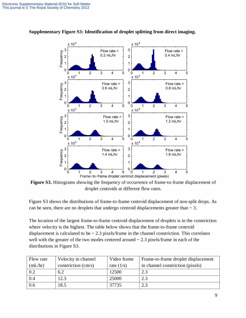
Supplementary Figure S3: Identification of droplet splitting from direct imaging.

Figure S3. Histograms showing the frequency of occurrence of frame-to-frame displacement of

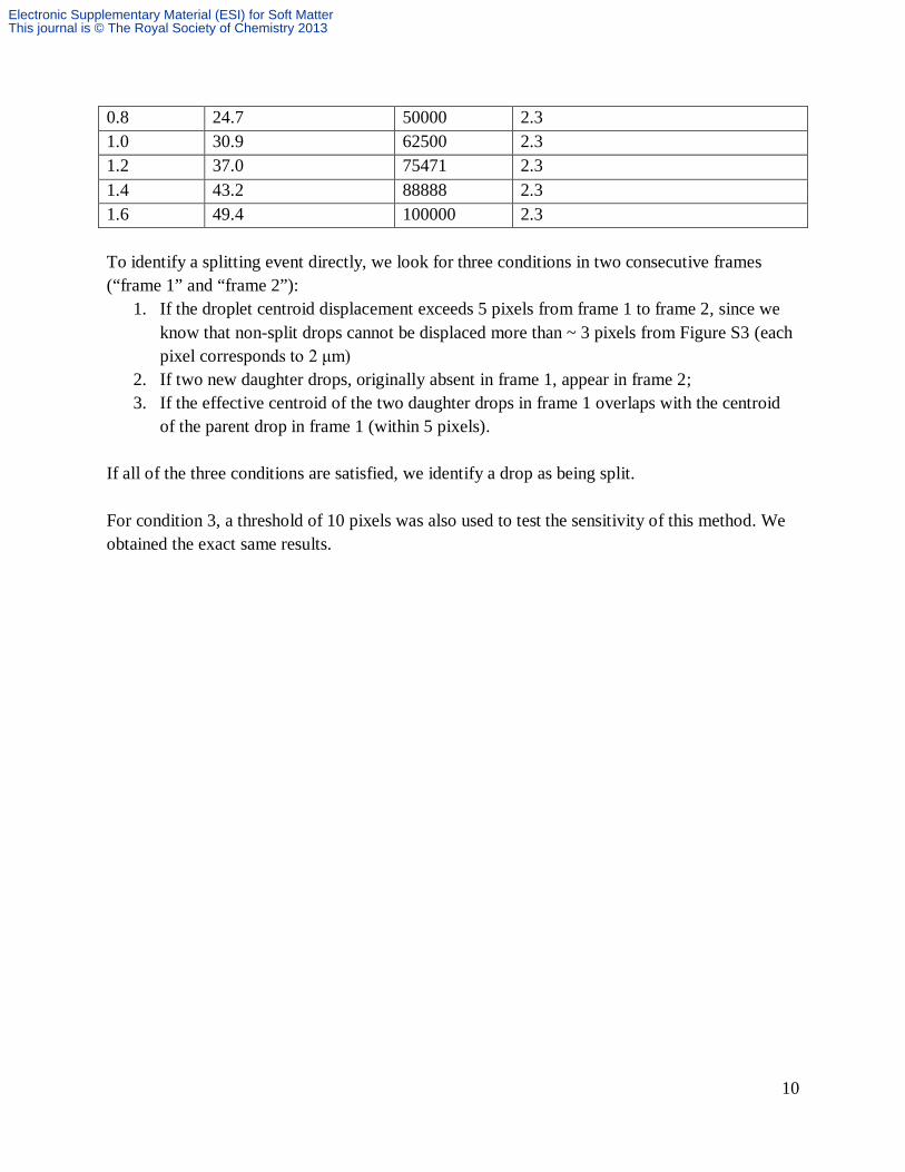
droplet centroids at different flow rates. Figure S3 shows the distributions of frame-to-frame centroid displacement of non-split drops. As can be seen, there are no droplets that undergo centroid displacements greater than ~ 3. The location of the largest frame-to-frame centroid displacement of droplets is in the constriction where velocity is the highest. The table below shows that the frame-to-frame centroid displacement is calculated to be ~ 2.3 pixels/frame in the channel constriction. This correlates well with the greater of the two modes centered around ~ 2.3 pixels/frame in each of the distributions in Figure S3. Flow rate (mL/hr)

Velocity in channel constriction (cm/s)

Video frame rate (1/s)

Frame-to-frame droplet displacement in channel constriction (pixels)

0.2 6.2 12500 2.3 0.4 12.3 25000 2.3 0.6 18.5 37735 2.3


10

0.8 24.7 50000 2.3 1.0 30.9 62500 2.3 1.2 37.0 75471 2.3 1.4 43.2 88888 2.3 1.6 49.4 100000 2.3 To identify a splitting event directly, we look for three conditions in two consecutive frames (“frame 1” and “frame 2”):

1. If the droplet centroid displacement exceeds 5 pixels from frame 1 to frame 2, since we know that non-split drops cannot be displaced more than ~ 3 pixels from Figure S3 (each pixel corresponds to 2 μm)

2. If two new daughter drops, originally absent in frame 1, appear in frame 2; 3. If the effective centroid of the two daughter drops in frame 1 overlaps with the centroid

of the parent drop in frame 1 (within 5 pixels).

If all of the three conditions are satisfied, we identify a drop as being split. For condition 3, a threshold of 10 pixels was also used to test the sensitivity of this method. We obtained the exact same results.


11

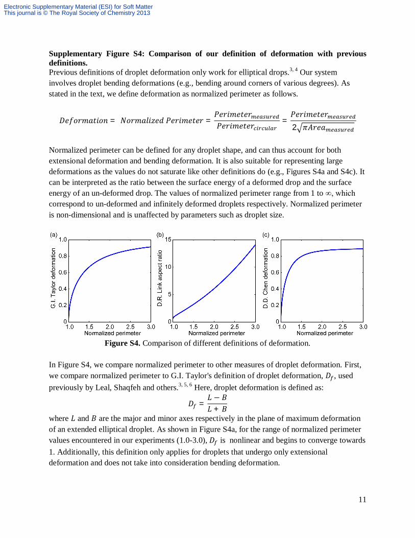
Supplementary Figure S4: Comparison of our definition of deformation with previous definitions. Previous definitions of droplet deformation only work for elliptical drops.3, 4 Our system involves droplet bending deformations (e.g., bending around corners of various degrees). As stated in the text, we define deformation as normalized perimeter as follows.

퐷푒푓표푟푚푎푡푖표푛 = 푁표푟푚푎푙푖푧푒푑푃푒푟푖푚푒푡푒푟 =푃푒푟푖푚푒푡푒푟푃푒푟푖푚푒푡푒푟 =

푃푒푟푖푚푒푡푒푟2 휋퐴푟푒푎

Normalized perimeter can be defined for any droplet shape, and can thus account for both extensional deformation and bending deformation. It is also suitable for representing large deformations as the values do not saturate like other definitions do (e.g., Figures S4a and S4c). It can be interpreted as the ratio between the surface energy of a deformed drop and the surface energy of an un-deformed drop. The values of normalized perimeter range from 1 to ∞, which correspond to un-deformed and infinitely deformed droplets respectively. Normalized perimeter is non-dimensional and is unaffected by parameters such as droplet size.

Figure S4. Comparison of different definitions of deformation.

In Figure S4, we compare normalized perimeter to other measures of droplet deformation. First, we compare normalized perimeter to G.I. Taylor's definition of droplet deformation, 퐷 , used previously by Leal, Shaqfeh and others.3, 5, 6 Here, droplet deformation is defined as:

퐷 =퐿 − 퐵퐿 + 퐵

where 퐿 and 퐵 are the major and minor axes respectively in the plane of maximum deformation of an extended elliptical droplet. As shown in Figure S4a, for the range of normalized perimeter values encountered in our experiments (1.0-3.0), 퐷 is nonlinear and begins to converge towards 1. Additionally, this definition only applies for droplets that undergo only extensional deformation and does not take into consideration bending deformation.


12

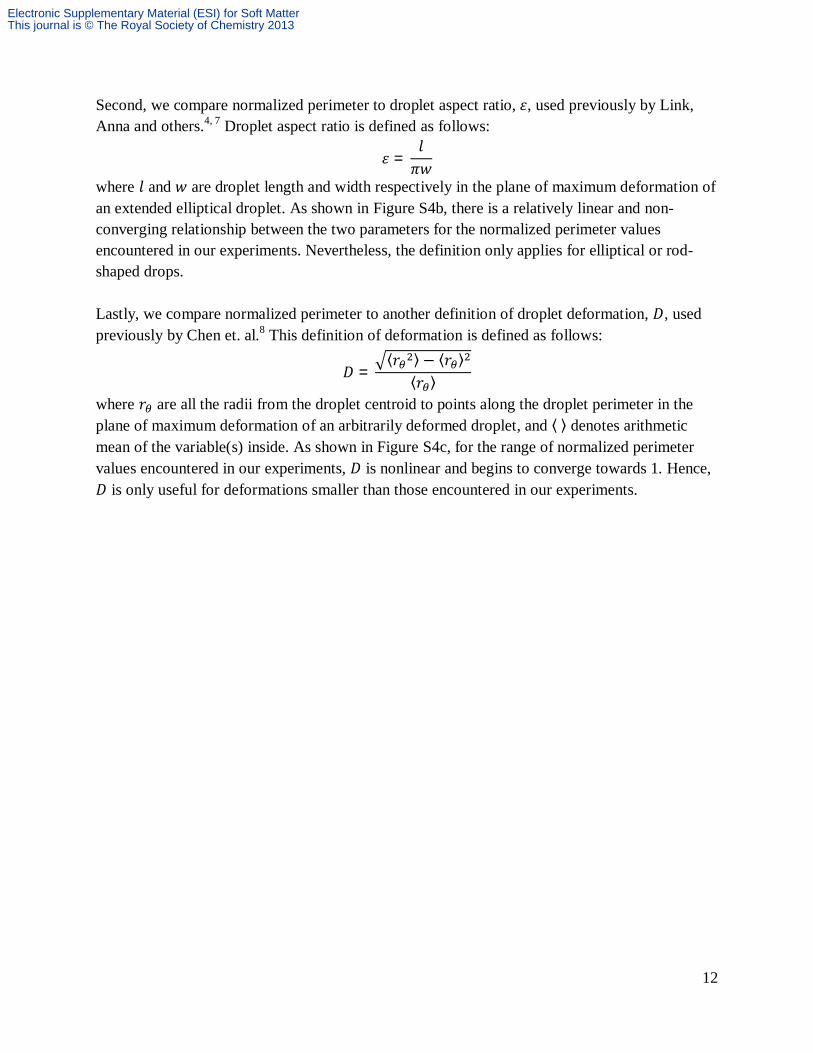
Second, we compare normalized perimeter to droplet aspect ratio, 휀, used previously by Link, Anna and others.4, 7 Droplet aspect ratio is defined as follows:

휀 =푙휋푤

where 푙 and 푤 are droplet length and width respectively in the plane of maximum deformation of an extended elliptical droplet. As shown in Figure S4b, there is a relatively linear and non-converging relationship between the two parameters for the normalized perimeter values encountered in our experiments. Nevertheless, the definition only applies for elliptical or rod-shaped drops. Lastly, we compare normalized perimeter to another definition of droplet deformation, 퐷, used previously by Chen et. al.8 This definition of deformation is defined as follows:

퐷 =⟨푟 ⟩ − ⟨푟 ⟩

⟨푟 ⟩

where 푟 are all the radii from the droplet centroid to points along the droplet perimeter in the plane of maximum deformation of an arbitrarily deformed droplet, and ⟨⟩ denotes arithmetic mean of the variable(s) inside. As shown in Figure S4c, for the range of normalized perimeter values encountered in our experiments, 퐷 is nonlinear and begins to converge towards 1. Hence, 퐷 is only useful for deformations smaller than those encountered in our experiments.


13

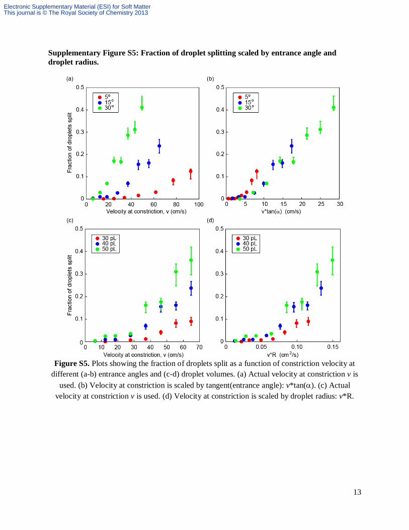
Supplementary Figure S5: Fraction of droplet splitting scaled by entrance angle and droplet radius.

Figure S5. Plots showing the fraction of droplets split as a function of constriction velocity at

different (a-b) entrance angles and (c-d) droplet volumes. (a) Actual velocity at constriction v is used. (b) Velocity at constriction is scaled by tangent(entrance angle): v*tan(). (c) Actual

velocity at constriction v is used. (d) Velocity at constriction is scaled by droplet radius: v*R.


14

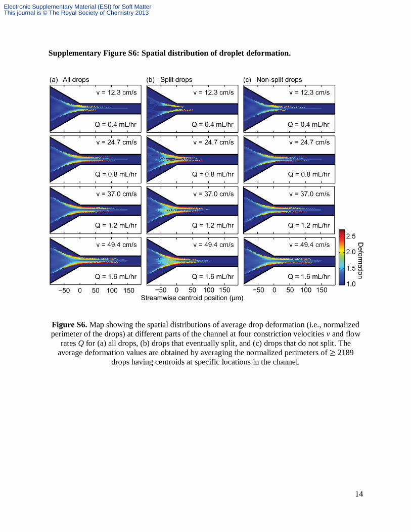
Supplementary Figure S6: Spatial distribution of droplet deformation.

Figure S6. Map showing the spatial distributions of average drop deformation (i.e., normalized perimeter of the drops) at different parts of the channel at four constriction velocities v and flow

rates Q for (a) all drops, (b) drops that eventually split, and (c) drops that do not split. The average deformation values are obtained by averaging the normalized perimeters of ≥ 2189

drops having centroids at specific locations in the channel.


15

References 1. W. Lee, L. M. Walker and S. L. Anna, Phys. Fluids, 2009, 21, 032103. 2. A. S. Basu, Lab Chip, 2013, 13, 1892-1901. 3. G. I. Taylor, Proc. R. Soc. A, 1934, 146, 0501-0523. 4. D. R. Link, S. L. Anna, D. A. Weitz and H. A. Stone, Phys. Rev. Lett., 2004, 92, 4. 5. S. Kaura and L. G. Leal, J. Rheol.,2010, 54, 981-1008. 6. A. B. Mosler and E. S. G. Shaqfeh, Phys. Fluids, 1997, 9, 3209-3226. 7. G. F. Christopher, J. Bergstein, N. B. End, M. Poon, C. Nguyen and S. L. Anna, Lab

Chip, 2009, 9, 1102-1109. 8. D. D. Chen, K. W. Desmond and E. R. Weeks, Soft Matt., 2012, 8, 10486-10492.


Documents

Electronic Supplementary Information Supplementary Information ... Naming convention of the video files: ... We have not measured the 3-phase contact angle of the drop at the PDMS