Electronic differential for high-performance electricreza.hoseinnezhad.com/papers/Andy_IJEHV_preprint.pdfElectronic differential for high-performance electric vehicles with independent

Electronic differential for high-performance electricvehicles with independent driving motors

Chunyun FuReza Hoseinnezhad*Alireza Bab-HadiasharReza N. JazarSimon Watkins

School of Aerospace, Mechanical and Manufacturing EngineeringRMIT UniversityPlenty Road, Bundoora, Victoria 3083, AustraliaE-mail: [email protected]: [email protected]: [email protected]: [email protected]: [email protected]*Corresponding author

Abstract: This paper presents a novel electronic differential design for high-performance electric vehicles with independent driving motors. The aim of thisdesign is to achieve neutral-steer in intense driving scenarios. The proposedmethod employs a closed-loop control system that constantly regulates the torquecommands sent to the independent driving motors. These commands are generatedto tune the torque difference between left and right driving motors at the amountthat leads to neutral-steer. Real vehicle parameters and real tyre testing dataare employed in extensive simulations. Simulation results demonstrate that thenew electronic differential works in principle and can endow the electric vehiclewith a next-to-neutral steer characteristic, which is of great significance tohigh-performance vehicles in challenging driving conditions. Also, comparativesimulations demonstrate how the proposed method can outperform competingmethods in terms of steering performance in various scenarios, while maintainingthe dynamic stability of the vehicle.

Keywords: electric vehicle; electronic differential; yaw rate control; neutral steer;independent driving motors.

Reference to this paper should be made as follows: Fu, C., Hoseinnezhad, R.,Bab-Hadiashar, A., Jazar, R.N. and Watkins, S. (2014) ‘Electronic differentialfor high-performance electric vehicles with independent driving motors’, Int. J.Electric and Hybrid Vehicles, Vol. x, No. x, pp.xxx–xxx.

Biographical notes: Chunyun Fu received his Bachelor’s degree from the Collegeof Mechanical Engineering, Chongqing University in 2006. He is currently aPhD candidate at the School of Aerospace, Mechanical and ManufacturingEngineering, RMIT University. His research interests include vehicle dynamicsand control, electric vehicles with independent driving motors and non-linear

2 Electronic differential for high-performance electric vehicles . . .

control applications on vehicle dynamics.

Reza Hoseinnezhad received the B.Sc., M.Sc., and Ph.D. degrees in electricalengineering from the University of Tehran, Tehran, Iran, in 1994, 1996, and 2002,respectively. During 2002–2010, he has held various positions at the Universityof Tehran, Swinburne University of Technology, Hawthorn, Australia, and theUniversity of Melbourne, Melbourne, Australia. He is currently a Senior Lecturerat the School of Aerospace, Mechanical and Manufacturing Engineering, RMITUniversity, Bundoora, Australia. He is the holder of two international patents andhas over 50 papers published in reputable journals and conferences. His mainresearch interests are vehicular electronics, multi-target tracking, and robustestimation in computer vision.

Alireza Bab-Hadiashar received the BSc degree in mechanical engineeringfrom Tehran University (1988), MES degree in mechanical and mechatronicsengineering from The University of Sydney (1993) and the PhD degree incomputer vision from Monash University (1997). His main research interests arethe development of robust estimation and segmentation techniques for computervision applications and intelligent and robust sensory systems for new generationvehicle technologies. He is currently a Professor with the School of Aerospace,Mechanical and Manufacturing Engineering at RMIT University, Melbourne,Australia. He has made a significant contribution to developing and establishingthe Mechatronics Engineering degree program at both Australia and Malaysiaand has published several highly cited papers in optical flow, robust segmentationand model selection techniques.

Reza N. Jazar is a professor of mechanical engineering, receiving his master’sdegree from Tehran Polytechnic in 1990, specializing in robotics. In 1997, heacquired his PhD from Sharif Institute of Technology in nonlinear dynamicsand applied mathematics. Prof. Jazar is a specialist in classical and nonlineardynamic systems, and has extensive experience in the field of vehicle dynamicsand mathematical modeling. Prof. Jazar has formulated many theorems,innovative ideas, and discoveries in classical dynamics, robotics, control, andnonlinear vibrations. Razi Acceleration, Theory of Time Derivative, Order-FreeTransformations, Caster Theory, Autodriver Algorithm, Floating-Time Method,Energy-Rate Method, and RMS Optimization Method are some of his discoveriesand innovative ideas. Prof. Jazar has authored 10 books all among the mostprestigious publications in their fields. Prof. Jazar’s Vehicle Dynamics has beenadopted by more than 50 universities worldwide. Prof. Jazar has written over200 scientific papers and technical reports.

Simon Watkins received his PhD degree from RMIT University in 1990.He is currently a professor with the School of Aerospace, Mechanical andManufacturing Engineering, RMIT University. Prof. Watkins’ main researchinterest lies in Micro Air Vehicles (MAV). He leads a research group in this areawith funding from the USAF supporting several PhD students, and he has alreadysuccessfully supervised more than twenty PhD or MEng students. Prof. Watkinshas published numerous prestigious peer-reviewed journal and conference papers,and has authored four book chapters. He was the originator and architect of thefirst automotive engineering degree in Australia, and set up RMIT racing whichwon the FISITA Formula Student World Cup in UK in 2007 and the AmericanFSAE event in 2006. He now supervises the design, build and testing of all-electricFSAE cars at RMIT.

C. Fu et al 3

1 Introduction

The swift responsiveness of electric actuators compared to hydraulic and mechanicalactuators, has already motivated many drive-by-wire technologies developed for differentcontrol purposes in internal combustion engine (ICE) vehicles (Hoseinnezhad & Bab-Hadiashar 2005, Hoseinnezhad et al. 2008, Hoseinnezhad & Bab-Hadiashar 2006). Whenit comes to electric vehicles (EVs), the vehicle locomotion is sourced by powerful electricmotors instead of ICEs. This makes EVs a promising solution to deteriorating global energyand environmental problems (Zhao & Zhang 2009, Magallán et al. 2009, Lebeau et al. 2013,Özel et al. 2013). Besides their energy and environmental benefits, due to the use of electricmotors, electric cars present significant performance advantages over ICE vehicles. Thesemerits can remarkably enhance vehicle dynamic performances. Some of the advantages ofelectric vehicles over ICE vehicles are as follows (Yin et al. 2009, Hori 2004, Geng et al.2009):

• Swift and accurate torque generation: this is the most straightforward advantage gainedfrom using electric motors instead of an ICE.

• Ease in designing an optimal control system: this is mainly due to the feasibility andease of accurate measurement of different dynamic states (such as the driving torque).

• Ease in designing a direct yaw moment control system such as an electronic differential,due to the feasibility of independent-driving-motor configuration.

High-performance electric vehicles equipped with independent driving motors,such as electric race cars, have recently gained attention, along with the advent ofFormula SAE/Formula student electric competitions in Australia, Italy, the UK andGermany (Watkins & Samsons 2011). With the independent-driving-motor configuration,the conventional mechanical differential is eliminated, and an appropriate electronicdifferential for electric vehicles is needed to control the independent torque outputs properly.Although utilisation of an electronic differential contributes to savings in fuel consumptionthrough reduction in mass, the major significance of electronic differential lies in theenhancement in handling, maneuverability and responsiveness of the electric vehicle.

Most existing electronic differential solutions are designed for passenger carapplications with the focus to maintain the vehicle stability as the first priority. However,in high-performance vehicle design, the main concerns, apart from vehicle stability, arethe cornering agility and responsiveness of the vehicle as well as the driver’s steering feel.Ideally, a high-performance vehicle needs to be neutral-steer (avoiding over- or under-steer)in intense driving conditions. This paper focuses on devising a proper electronic differentialthat achieves this goal.

A complete set of non-linear equations is firstly presented to describe the eight degreesof freedom vehicle motion, including rolling. Then, this set of equations are appropriatelysimplified to provide illuminating implications for controller design. The designed controllergenerates the desired motor torque difference between the driving motors that leads toneutral-steer.

In extensive simulations, we compare the steering performance of a typical electric racecar equipped with the proposed electronic differential, with three other popular solutions.The results demonstrate that our method endows the race car with a close-to-neutral steercharacteristic while maintaining its stability in challenging steering scenarios, whereas thecompeting methods fail to keep the car close to neutral-steer.


The outline of this paper is as follows. In section 2, we present the background inwhich the working principles of the three popular electronic differential control solutionsare reviewed. We then present the vehicle mathematical model in section 3 and the proposedcontroller design in section 4. Comparative simulations are presented in section 5, followedby conclusions in section 6.

2 Background

Different electronic differential control methods have been proposed in the literature. Here,we introduce the three most popular methods and briefly explain the concepts and principlesbehind these methods. In section 5, the control performance of these popular methods willbe analysed in comparison with our proposed method.

2.1 Equal torque method

A straightforward solution for electronic differential control is to emulate the behaviour ofan open differential, the most used mechanical differential, by applying equal torques to thetwo driving wheels, as shown in Figure 1 (Magallán et al. 2008, 2009). This method providesthe electric vehicle with a cornering performance similar to an ICE vehicle equipped withan open differential. In this design, the torque commands sent to the motors are determinedbased on the difference between the speed required by the driver (read from the accelerationpedal and denoted by ω∗ in Figure 1) and the average of the two driving wheel speeds(denoted by ω in Figure 1). The speed error is then used by a PI controller to generate equaltorque reference for the two motor controllers.

When a car is at low speed and does not have wheel slips, the average of the two drivingwheel speeds is proportional to the vehicle longitudinal speed and the open differentialbehaviour is reproduced by the equal torque method (Magallán et al. 2008, 2009). However,when the car is running very fast or in driving conditions involving relatively high wheelslips, the average of the two driving wheel speeds is no longer proportional to the vehiclelongitudinal speed. As a result, the equal torque method would not generate proper drivingcommands. For instance, when one driving wheel is locked, the other one will be sped upto twice the reference speed (Magallán et al. 2008, 2009), resulting in severe tyre slip andundesirable yaw moment.

2.2 Ackerman method

Unlike the equal torque method, Hartani et al. (2008) proposed a control algorithm thatemploys independent reference signals to control two separate driving motors. The proposedmethod uses the vehicle speed and the steering angle as input parameters and calculatesthe required inner and outer wheel angular speeds, by means of the well-known Ackermansteering geometry. The Ackerman geometry, as a simple kinematic condition, has beencommonly employed in various electronic differential designs (Haddoun et al. 2008, Zhao,Zhang & Guan 2009, Lee et al. 2000, Perez-Pinal et al. 2009, Zhou et al. 2007).

In Ackerman steering geometry, the driving wheels are assumed to turn slip-free, andthe desired angular velocities of the two driving wheels are given by:

ωL =vLR

=v

R(1 − d tan δ

2l) (1)

C. Fu et al 5

ωR =vRR

=v

R(1 +

d tan δ

2l), (2)

where v denotes the vehicle velocity at the centre of the rear axle, R represents the tyreradius, d denotes the rear track, l is the wheel-base and δ is the steering angle of the frontwheels.

Maintaining the wheel angular velocities at the above desired levels is the main objectiveof many existing electronic differential control methods. When the electric vehicle entersa corner, the electronic differential acts immediately on both motors, reducing the angularvelocity of the inner wheel while increasing that of the outer wheel (Hartani et al. 2008) totheir desired values defined by equations (1) and (2).

In our simulations, to examine the performance of methods developed on the basis ofsatisfying Ackerman condition, we have tuned the driving wheel angular velocities basedon their sum and difference, with the sum being proportional to the speed command readfrom the throttle pedal sensor and the difference computed from equations (1) and (2):

∆ω = ωR − ωL =vd tan δ

Rl. (3)

It is important to note that the Ackerman steering geometry is a purely kinematiccondition that is accurate only when the wheel slip is very low. However, in intense drivingconditions (for example in racing condition), vehicles run very fast and wheel slips areinevitable and ubiquitous. Indeed, in challenging driving conditions sometimes some levelof wheel slip is necessary for best maneuverability. Thus, control designs based on satisfyingAckerman condition are normally suitable for low-speed passenger car applications in whichtyre slips are assumed to be negligible during steering. Results of our simulations willexpose the inherent shortcomings of Ackerman condition-based electronic differentials.

2.3 Karogal’s method

As described above, neither the equal torque method nor the Ackerman method takes intoaccount the vehicle dynamics. Some modern electronic differential control designs havebeen proposed in which besides the vehicle kinematics, its dynamics is also incorporated.By taking the vehicle dynamics into consideration, such control methods aim to produceresponsive driving commands while keeping the car within its physical limits. Kim & Kim(2007) proposed a controller design that maintains the yaw rate of the vehicle at a desiredlevel determined by a planar vehicle dynamic model. Similarly, Karogal & Ayalew (2009)put forward an independent torque distribution method in which again a planar dynamicmodel is used to derive the desired reference value for the control system. A vehicle planarmodel was also employed by Zhao, Zhang & Zhao (2009) to obtain the desired yaw ratein their direct yaw-moment control (DYC) algorithm for a four-in-wheel-motor electricvehicle.

In the above control methods, the planar model is mainly used to derive the desired yawrate which is indeed the steady-state yaw rate expressed in the following general form:

r =vxδ

l(1 +Kvx2), (4)


where vx denotes the vehicle longitudinal velocity, l represents the wheel-base and K iscalled the “stability factor” given by:

K =m

l2(lfCαr

− lrCαf

), (5)

where m is the total vehicle mass, lf and lr are the distance from the centre of gravity to thefront and rear axle respectively, and Cαf , Cαr are the cornering stiffness of the front andrear tyres respectively. In the above designs, the stability factorK is maintained at a positivevalue to ensure the stability of the vehicle. However, a positive stability factor causes under-steer and gives the vehicle a sluggish cornering response, which compromises the handlingof high-performance vehicles. In contrast, a negative stability factor produces over-steerthat may lead to instability, particularly when novice drivers drive. In the following text,we will present how the ideal steer characteristic, neutral-steer, can be realised for a high-performance electric vehicle, without compromising vehicle stability.

3 Vehicle equations of motion

Consider a rear-wheel-drive electric vehicle with a local coordinate frame attached to itscentre of mass, as schematically shown in Figure 2. The x-axis is the centreline of thevehicle and points forwards, while the y-axis points to the left. The x-y plane is parallel tothe ground, and the z-axis is perpendicular to the x-y plane and points upwards. The originof the coordinate system is at the vehicle centre of mass (C).

Using the aforesaid local coordinate system, the vehicle dynamics can be expressed bythe following equations:

∑Fx =mvx −mrvy∑Fy =mvy +mrvx∑Mx = Ixp∑Mz = Iz r,

(6)

where,

m = vehicle mass,vx = longitudinal velocity of the centre of mass,vy = lateral velocity of the centre of mass,p = roll rate,r = yaw rate,Ix = roll moment of inertia, andIz = yaw moment of inertia.

In most relevant literature, a planar vehicle model without the vehicle roll motion is usedin vehicle handling analysis. However, in the above set of equations, we take into accountthe vehicle roll motion, in order to provide more accurate and realistic results.

C. Fu et al 7

Expanding the left-hand side of the equations in (6), we obtain:

∑Fx =

4∑i=1

(Fxi cos δi − Fyi sin δi)∑Fy =

4∑i=1

(Fxi sin δi + Fyi cos δi)∑Mx = −

4∑i=1

zi(Fxi sin δi + Fyi cos δi) +Mk +Mc∑Mz =

4∑i=1

xi(Fxi sin δi + Fyi cos δi)−4∑i=1

yi(Fxi cos δi − Fyi sin δi),

(7)

where xi, yi and zi represent the coordinates of the i-th wheel, δi denotes the wheel steeringangle of the i-th wheel (δ3 = δ4 = 0),Mk andMc are the roll moment produced by springsand dampers of the suspension system respectively, and Fxi and Fyi are the longitudinaland lateral road-tyre reaction force exerted on the i-th wheel, respectively.

The roll moments Mk and Mc can be further expressed by the equations below:

Mk = −kϕϕMc = −cϕϕ = −cϕp, (8)

where the coefficients kϕ and cϕ are the total roll stiffness and the total roll damping of thevehicle suspension system, and ϕ denotes the roll angle of the vehicle.

The longitudinal and lateral road-tyre reaction forces, Fxi and Fyi, are non-linearlyrelated to the wheel longitudinal slip ratio s and the wheel side-slip angle α, respectively.These relationships are elaborated by the well-known Magic Formula equations (Pacejka2006) which have been frequently used in vehicle dynamic and control literature suchas Mutoh et al. (2008), Mutoh & Nakano (2012), Hu et al. (2012):

y(x) = D sin(C tan−1(Bx− E(Bx− tan−1Bx))) (9)

with

Y (X) = y(x) + SVx=X + SH

(10)

where,

Y (X) = output variable Fxi or Fyi,X = input variable tanα or slip ratio s,B = stiffness factor,C = shape factor,D = peak value,E = curvature factor,SH = horizontal shift, andSV = vertical shift.


Utilising the above Magic Formula, the following torque equilibrium equation for thedriving wheels is established:

T = Jdω

dt+ FxR, (11)

where T is the motor driving torque, J represents the moment of inertia of the drivingwheel assembly, ω and R denote the wheel angular velocity and radius, Fx stands for thelongitudinal road-tyre reaction force.

Equations (6)-(11) constitute a complete non-linear vehicle dynamic model whichthoroughly describes the eight degrees of freedom vehicle motion. We employ this completemodel to simulate a full vehicle in our comparative simulation studies in MATLAB Simulinkenvironment, as will be presented in section 5.

4 Electronic differential design

4.1 Equations of motion linearisation

In order to reveal the fundamental mathematical relationships that govern the vehicledynamics with electronic differential on-board, we now investigate the implications deducedfrom the aforesaid equations (6)-(11). When the wheel side-slip angle α is small, the MagicFormula equation for lateral force can be considered linearly proportional toα, which reads:

Fy = −Cαα (12)

where Cα is called the cornering stiffness of the tyre. When a vehicle rolls, it is knownthat the wheel camber angle will change which in turn results in a tyre camber thrust.To accommodate the effect of camber angle, a new term is added to the tyre lateral forceequation:

Fy = −Cαα− Cϕϕ (13)

where Cϕ is the tyre camber thrust coefficient and ϕ is the vehicle roll angle (Jazar 2008).The side-slip angle of the i-th wheel αi can be expressed by the following equation,

assuming that β, δi and αi are small (Jazar 2008):

αi = β + xir

vx− Cβi

p

vx− δi − Cδϕiϕ, (14)

whereCβi is called the tyre roll rate coefficient,Cδϕiϕ represents the steering angle causedby the vehicle roll motion, and Cδϕi is called the roll steering coefficient. It is worth notingthat the rear wheel steering angles δ3 and δ4 are zero, and the cot-average of the front wheelsteering angles, δ, is used in place of δ1 and δ2 for simplicity (cot δ = (cot δ1 + cot δ2)/2).

We then assume that the left and right longitudinal forces are symmetric, namely Fx1 =Fx2 andFx3 = Fx4. We also assume that δi is small, then we have approximations sin δi ≈ 0and cos δi ≈ 1. Combining equations (6)-(14) leads to the following equations that governthe lateral, yaw and roll motion of the car:

Crr + Cpp+ Cββ + Cϕϕ+ Cδδ =mvy +mrvxDrr +Dpp+Dββ +Dϕϕ+Dδδ = Iz rErr + Epp+ Eββ + Eϕϕ+ Eδδ = Ixp,

(15)

C. Fu et al 9

where,β = side-slip angle,ϕ = roll angle, andδ = front wheel steering angle.

The detailed derivation of the above equations, and the coefficients that appear on theleft-hand side of the equations are explicitly expressed in Jazar (2008). The coefficientsare rewritten in the Appendix. The equation for longitudinal dynamics is neglected here,because in vehicle handling analysis the vehicle longitudinal velocity vx is always assumedto be constant, i.e. vx = 0.

We have employed small angle assumption several times in the above derivations. It isvery important to justify that in intense driving conditions, the simplified vehicle model (15)obtained by using small angle assumption does not lose its validity.

The application of small angle assumption toα can be justified by an example in Milliken& Milliken (1995), a typical racing tyre inflated at 31 psi for a given load of 1800 lb. ThisGoodyear racing tyre provides the maximum lateral force at a side-slip angle of about 6.5◦

after which the tyre enters the unstable frictional range. We notice that 6.5◦ is only about0.1 rad and the tyre normally operates in the range below 6.5◦, which enables us to safelyapply small angle assumption in the linearisation.

As for δ, with a steering ratio of 1:12, a small front wheel steering angle of 0.2 rad iscorresponding to a steering wheel/column angle of about 138◦. At a medium vehicle speed,say 60 km/h, this steering angle is a typical marginal magnitude beyond which vehiclestend to lose stability. So in the stable region, the vehicle will mostly operate with a smallersteering angle at that speed, which in turn makes it justified to apply small angle assumptionto the front wheel steering angle δ.

Besides, when both α and δ are assumed to be small, the associated vehicle side-slipangle β becomes small as well. Summing up the above points, the vehicle model (15)obtained by means of small angle assumptions does not lose its validity, and can capture themajor characteristics of vehicle dynamics. As we will present in the next section, this modelprovides us with fundamental understanding of the relationships between the yaw rate andthe left-right torque difference, based on which our electronic differential is designed.

4.2 Controller design

Our design is based on independently generating different torque commands to be sent tothe two driving motors. Different motor torques are intuitively expected to lead to differentroad-tyre reaction forces on the left and right driving wheels, denoted by Fx3 and Fx4. Inthis section, using the vehicle motion equations presented in section 4.1, we first derive theequation showing a direct relationship between the yaw rate and the difference in reactionforces ∆F = Fx3 − Fx4. We then show the relationship between the force difference andthe torque difference ∆T as mathematically inferred from the wheel dynamic equation.Combining the two relationships will show how the yaw rate can be directly controlled bytuning the torque difference.

We note that a force difference ∆F is equivalent to an additional moment ∆M =∆F × d/2 applied on the rear axle plus a force ∆F exerted at the centre of the driving (rear)


axle, as illustrated in Figure 3. Thus, in presence of the difference between the reactionforces, only the second equation in (15) needs to be modified as below:

Drr +Dpp+Dββ +Dϕϕ+Dδδ +d

2· ∆F = Iz r. (16)

Here, we note that the dynamics of the vehicle (its lateral, yaw and roll dynamics) issubstantially slower than the dynamics of the electric motors. Therefore, in the context ofcontrol command generation (torque commands sent to motors for generating particularvalues of torques), the time-derivative terms in the equations of motion are negligible andcan be discarded. Hence, for the purpose of controlling the driving motors, we can safelyuse the following steady-state forms of the motion equations:Cβ Cr −mvx Cϕ

Dβ Dr Dϕ

Eβ Er Eϕ

βrϕ

=

−Cδ 0−Dδ −d

2−Eδ 0

[ δ∆F

]. (17)

Solving the above system of equations, the following yaw rate response is derived in termsof the control inputs δ and ∆F :

r =ZδZ0δ +

ZFZ0

∆F, (18)

where,

ZF = d2 (EβCϕ − EϕCβ)

Z0 =Eβ(DϕCr −DrCϕ −mvxDϕ)+Eϕ(DrCβ −DβCr +mvxDβ)+Er(DβCϕ −DϕCβ)

Zδ =Eβ(DδCϕ −DϕCδ) + Eϕ(DβCδ −DδCβ)+Eδ(DϕCβ −DβCϕ).

(19)

Equation (18) shows a direct relationship between the yaw rate and ∆F .As mentioned above, compared to the dynamics of the electric motors, the dynamics of

the mechanical parts is very slow. Particularly, during each sampling time of the electroniccontrol system, the variation of the wheel angular velocity is negligible. Thus, equation (11)can be simplified to:

T = FxR. (20)

This shows that longitudinal road-tyre reaction forces (and their difference) can be directlycontrolled by tuning the torque commands sent to the driving motors.

Substituting (20) in (18) leads to:

r =ZδZ0δ +

ZFZ0R

∆T. (21)

Equation (21) clearly demonstrates a direct relationship between the yaw rate and thedifference in the two motor torques. This implies that, by controlling the two motor torques,we can tune the vehicle steady-state yaw rate to attain its desired value.

C. Fu et al 11

To calculate the desired yaw rate, we consider the main criterion for neutral-steerbehaviour: the vehicle’s instantaneous turning radius should not change with speed. Thevehicle will be under-steer if its turning radius increases upon acceleration, and over-steerif it decreases upon acceleration. Kinematically, the turning radius is known as ρ = v/r,where v is the resultant velocity at the centre of mass. We assume that the lateral componentof v is negligible compared to its longitudinal component vx, i.e. ρ = vx/r.

In numerator of the fraction in equation (4), we substitute vx with rρ, and solving for ρwe have:

ρ =l(1 +Kvx

2)

δ. (22)

For ρ to be invariant with vx, we need the Kvx2 term to vanish. Hence, the desired yawrate of a neutral-steer vehicle is:

r∗ =vxlδ. (23)

It has already been shown in (21) that the steady-state yaw rate is a function of the motortorque difference. According to (21), the controller should be designed to achieve a desiredyaw rate by creating a corresponding desired motor torque difference ∆T ∗, namely:

r∗ =ZδZ0δ +

ZFZ0R

∆T ∗. (24)

Subtracting equation (21) from equation (24), we obtain the following relationship expressedin terms of errors in ∆T and r:

∆T ∗ − ∆T =Z0R

ZF(r∗ − r). (25)

Note that the electronic differential system is a discrete control system. The output of thecontroller ∆T (k + 1) at discrete time k + 1, must be generated to make r(k) approachr(k)∗ as soon as possible. Thus, our control policy is to create ∆T (k + 1) = ∆T ∗ whichleads to:

∆T (k + 1) − ∆T (k) =Z0R

ZF(r(k)∗ − r(k)). (26)

Dividing both sides by the sampling time ts, we obtain:

∆T (k + 1) − ∆T (k)

ts=Z0R

ZF ts(r(k)∗ − r(k)). (27)

Since the sampling time ts is very small, the left-hand side of equation (27) can be consideredas the time-derivative of the torque difference ∆T . Therefore, integration of both sides ofequation (27) in continuous time t yields:

∆T (t) =Z0R

ZF ts

∫ t

0

eβ(τ)dτ, (28)


where,

eβ(τ) = r(τ)∗ − r(τ). (29)

Equation (28) implies that the desired torque difference between the two driving motorscan be attained by using a simple I controller. We recall that the Simulink model usedfor simulation studies employs a complete set of non-linear equations, as mentioned insection 3. However, we utilised a set of linearised and simplified equations to achieve theabove controller design. To accommodate the modelling errors and better regulate the yawrate, we propose a PID controller instead of just an I controller for the proposed electronicdifferential.

Figure 4 shows the block diagram of the proposed electronic differential. The electronicdifferential controller consists of two controller units. As explained above, the PID formyaw rate controller unit compares the actual yaw rate with the desired yaw rate measuredbased on equation (23) and generates half the difference in torque commands, ∆T/2. Thespeed controller unit, also suggested in PID form, provides the base torque Tbase which isthe average of the two torque commands on the left and right sides, TL and TR. We tunethe base torque in such a way that the vehicle longitudinal velocity, vx, follows the desiredspeed read from the throttle pedal sensor (Karogal & Ayalew 2009).

The parameters of both controllers can be easily tuned by trial-and-error. The outputsof the two controllers are subtracted and summed up to form the torque commands sent tothe left and right inverters. The saturation blocks model the physical limits to the extentof torque the motors can generate. The two inverters convert torque commands to electricsignals to drive the motors, using the feedback phase signal φ read from the motor encoders.Two brush-less permanent-magnet DC motors are selected as driving motors, which allowsboth positive and negative torques to be generated. Several sensors are employed to measurethe vehicle states r, vx (the average linear velocity of the two passive wheels is taken as thevehicle longitudinal velocity vx) and the driver’s commands v∗x, δ. These signals are fedback to form the errors for the two PID controller units.

5 Simulation

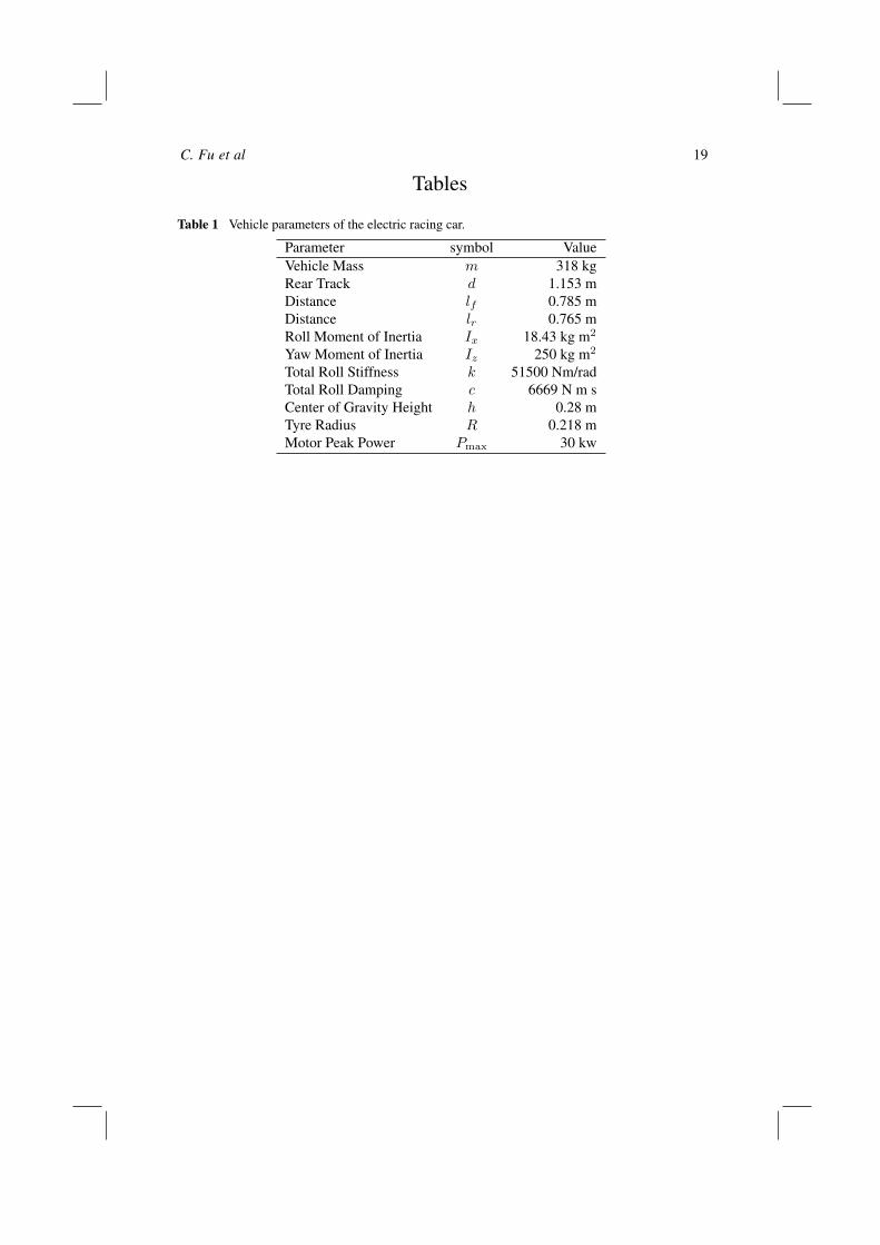
A set of simulations are conducted in MATLAB Simulink environment to verify theeffectiveness of the proposed electronic differential design and compare the steeringperformances between the competing methods. As mentioned in section 3, a complete non-linear vehicle dynamic model is employed for simulation studies. The vehicle parametersused in our simulations are from a real electric racing car built at our institution as shown inFigure 5. This car is the third generation of electric racing cars designed and developed byour students, equipped with two independent driving motors for rear wheels. The vehicleparameters are listed in Table 1. As our institution is a member of the Formula SAE TyreTest Consortium (TTC), we obtained real tyre testing data from TTC and employed thosedata in Magic Formula for road-tyre reaction force calculation in our simulations (Kasprzak& Gentz 2006).

The proposed method is compared with several electronic differential control solutionsintroduced in section 2. These methods are equal torque method, Ackerman method andKarogal’s method. Our simulation studies comprise two groups: case studies with stepsteering inputs and case studies with sinusoidal steering inputs. In each group, we examine

C. Fu et al 13

the steering performance of a fully simulated vehicle in response to various magnitudes andfrequencies (for sinusoidal inputs) of the step/sinusoidal steering inputs.

The performance of each electronic differential control scheme can be evaluated interms of several criteria. In intense driving scenarios (such as racing conditions), the mostimportant criterion is the capability of tracking the desired yaw rate expressed by equation(23) which corresponds to neutral-steer. Secondly, vehicle paths are taken into consideration.These paths demonstrate how close the racing car is to the desired track, and they also act asa complement to the first criterion. Lastly, the slip ratio and the corresponding longitudinalroad-tyre reaction force of the inner driving wheel are assessed, in order to check if theelectronic differential system causes any instability to the vehicle maneuvres.

5.1 Simulation with step inputs

In this set of simulations, step inputs are used as steering inputs in different rounds to verifythe effectiveness of the proposed method. In each round, the same value of step input isapplied to all four competing control methods, but the value is varied between differentrounds. We have examined a large range of possible step magnitudes. For the sake of brevity,here we only present the results for step inputs δ = 0.1 rad, δ = 0.075 rad and δ = 0.05rad in three different rounds. The initial longitudinal velocity vx is set to be 16 m/s. In allrounds, the step steering command occurs at t = 10 s.

5.1.1 Step input δ = 0.1 rad

As is seen in Figure 6, the yaw rate errors of all other three methods converge to a non-zerovalue after a period of time, and only the proposed control method has been able to bring theyaw rate error to zero. In other words, in steady-state, only with our method does the vehicleachieve neutral-steer. As expected, the equal torque method performs the worst, as it alwaysoutputs the same torque commands to driving motors and emulates the behaviour of an opendifferential. We observe a pulse at t = 10 s for all these four curves. This happens becausethe slope of the step input at t = 10 s is infinity and all methods need time to converge. Att = 10 s, all methods have the same yaw rate error of slightly over 1 rad/s, but this errorfades out very quickly.

The vehicle paths using the aforesaid four control algorithms, after 12.5 s of simulation,are portrayed in Figure 7. It is evident that the path traversed with the proposed methodon-board is the closest to the desired vehicle track, which is consistent with the yaw rateerrors shown in Figure 6.

Figure 8 shows the slip ratio responses of the inner driving wheel using different controlmethods. The inner driving wheel normally presents the worst wheel slip because it isconsiderably unloaded by the centrifugal force during cornering. The slip ratios of theequal torque method and the Karogal’s method are both positive, while the slip ratios ofthe Ackerman method and the proposed method are negative. Moreover, the slip ratios ofall other three methods are very small in absolute value, compared to that of the proposedmethod. This result indicates that, the longitudinal road-tyre reaction forces generated bythe equal torque method and the Karogal’s method are positive (forward) and small, and theforce produced by the Ackerman method is negative (backward) and small. Only with theproposed method, can a large (in absolute value) negative (backward) longitudinal road-tyrereaction force be generated to decrease the yaw rate error. This explanation is verified byFigure 9 in which the values of the longitudinal forces generated on the inner driving wheelby different methods are clearly plotted. In fact, the about 6% (absolute value) slip ratio


exhibited by the proposed method is normally an optimal value for most tyres, at which,sufficient longitudinal road-tyre reaction force can be generated, and neither does this slipratio jeopardise vehicle safety nor causes any excessive tyre wear.

As mentioned before, with brush-less permanent-magnet DC motors, both positive andnegative torques can be generated. When motors generate negative torques, they are actuallyworking in the “electrical braking” mode (Mutoh 2012). We observe that, in Figure 9, theroad-tyre reaction force generated by the proposed method is negative, while the wheelangular velocity of the inner driving wheel seen from Figure 10 is positive. This meansthat the direction of the motor torque is opposite to the direction of angular velocity of thewheel, namely the motor is operating in the “electrical braking” mode. Since the vehiclelongitudinal velocity vx is maintained by the speed controller that generates the basetorque, vx will not be decreased due to this “electrical braking” motion. Furthermore, inthe “electrical braking” mode, regenerative braking can be made possible to enhance theefficiency of the driving system.

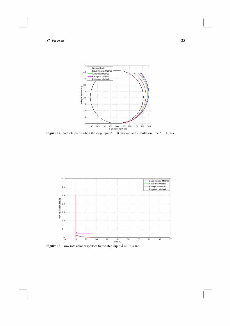
5.1.2 Step inputs δ = 0.075 rad and δ = 0.05 rad

The performances of the four competing methods when δ = 0.075 rad and δ = 0.05 rad aresimilar to those when δ = 0.1 rad, as can been seen in Figures 11–14. The proposed methodstill brings the yaw rate error down to zero, and keeps the vehicle path the closest to thedesired track. For brevity, the slip ratio responses and the longitudinal road-tyre reactionforce responses of the inner driving wheel for step input δ = 0.075 rad and δ = 0.05 radare omitted, but it is worth emphasising that they are similar to Figure 8 and Figure 9 andthe responses agree with the aforesaid explanation.

5.2 Simulation with sinusoidal inputs

In this group of simulations, sinusoidal signals are employed as steering inputs to the system.We have examined various combinations of magnitudes and frequencies for the steeringcommands. The results of four cases are presented here. In order to save space, we onlypresent the yaw rate tracking results.

Figure 15 displays the yaw rate error responses with the magnitude and frequency ofthe sinusoid being 0.1 rad and π rad/s, respectively. We observe that the proposed methodtracks the desirable yaw rate with errors considerably smaller than the competing methods.The error peak value presented by this method is approximately 0.1 rad/s lower than theequal torque method and 0.07 rad/s lower than the Ackerman method. Similar superiorperformance of the proposed method can also be observed from the yaw rate error plotspresented in Figure 16 (for steering input with amplitude of 0.1 rad and frequency of 0.5πrad/s), Figure 17 (for steering input with amplitude of 0.05 rad and frequency of π rad/s) andFigure 18 (for steering input with amplitude of 0.05 rad and frequency of 0.5π rad/s). Theobservations of the above figures demonstrate that the proposed method is able to keep thevehicle much closer to neutral-steer condition with challenging sinusoidal steering inputs.

In summary, the simulation results demonstrate that in response to sharp steeringdemands (in the form of large steps and large and fast sinusoids), the proposed methodoutperforms the competing methods in terms of steering performance. More precisely, forvarious magnitudes of the step input, our method consistently drives the yaw rate to convergeto the desired value, and keeps the vehicle the closest to the desired path. Meanwhile, noexcessive wheel slips occur on the inner driving wheel, which guarantees the stability of thevehicle maneuvres. When we employ sinusoidal steering inputs with different combinations

C. Fu et al 15

of amplitude and frequency, the proposed method shows the smallest yaw rate error, therebymaintaining the car the closest to neutral-steer characteristic.

6 Conclusions

A neutral-steer vehicle follows the driver’s command accurately and enables the driverto accelerate in a corner without constantly adjusting the steering wheel. This capabilityis of special significance to high-performance vehicles. With conventional mechanicaldifferentials or common electronic differential control solutions, it is almost impossible tomake a vehicle neutral-steer in intense driving conditions. In this paper, we mathematicallyand graphically demonstrated how neutral-steer can be made possible for high-performanceelectric vehicles with the proposed electronic differential system.

Simulation results manifest that with challenging steering inputs, using the proposedelectronic differential, the vehicle closely tracks the desired yaw rate that corresponds toneutral-steer, namely, a next-to-neutral steer characteristic is achieved. It is also shownin simulations that in various challenging steering scenarios, our electronic differentialoutperforms the common electronic differential control methods.

Appendix: Coefficients in motion equations

The coefficients of motion equations listed in (15) are given by the following equations.Interested readers are referred to Jazar (2008) for derivation details.

Cr =∂Fy∂r

= − lfvxCαf +

lrvxCαr

Cp =∂Fy∂p

=CαfCβfvx

+CαrCβrvx

Cβ =∂Fy∂β

= −(Cαf + Cαr)

Cϕ =∂Fy∂ϕ

= CαrCδϕr + CαfCδϕf − Cϕf − Cϕr

Cδ =∂Fy∂δ

= Cαf

Er =∂Mx

∂r= − lf

vxCTfCαf +

lrvxCTrCαr

Ep =∂Mx

∂p=

1

vxCβfCTfCαf +

1

vxCβrCTrCαr − cϕ

Eβ =∂Mx

∂β= −CTfCαf − CTrCαr

Eϕ =∂Mx

∂ϕ= −CTf (Cϕf − CαfCδϕf ) − CTr(Cϕr − CαrCδϕr) − kϕ

Eδ =∂Mx

∂δ= CTfCαf


Dr =∂Mz

∂r= −

l2fvxCαf −

l2rvxCαr

Dp =∂Mz

∂p=lfvxCβfCαf −

lrvxCβrCαr

Dβ =∂Mz

∂β= −lfCαf + lrCαr

Dϕ =∂Mz

∂ϕ= −lf (Cϕf − CαfCδϕf ) + lr(Cϕr − CαrCδϕr)

Dδ =∂Mz

∂δ= lfCαf

In the above equations, Cαf and Cαr are the cornering stiffness of the front and reartyres respectively. Cϕf and Cϕr denote the tyre camber thrust coefficient of the front andrear tyres respectively. Cδϕf and Cδϕf represent the tyre roll steering coefficient of thefront and rear tyres respectively. Cβf and Cβr stand for the tyre roll rate coefficient of thefront and rear tyres respectively.CTf andCTf are the overall torque coefficient of the frontand rear tyres respectively. kϕ is roll stiffness of the suspension system, and cϕ is the rolldamping of the suspension system.

References

Geng, C., Mostefai, L., Denai, M. & Hori, Y. (2009), ‘Direct yaw-moment control ofan in-wheel-motored electric vehicle based on body slip angle fuzzy observer’, IEEETransactions on Industrial Electronics 56(5), 1411 – 1419.

Haddoun, A., Benbouzid, M. E. H., Diallo, D., Abdessemed, R., Ghouili, J. & Srairi, K.(2008), ‘Modeling, analysis, and neural network control of an EV electrical differential’,IEEE Transactions on Industrial Electronics 55(6), 2286 – 2294.

Hartani, K., Bourahla, M., Miloud, Y. & Sekkour, M. (2008), ‘Direct torque control ofan electronic differential for electric vehicle with separate wheel drives’, Journal ofAutomotion & Systems Engineering 2(2).

Hori, Y. (2004), ‘Future vehicle driven by electricity and control - research on four-wheel-motored “UOT Electric March II”’, IEEE Transactions on Industrial Electronics51(5), 954 – 962.

Hoseinnezhad, R. & Bab-Hadiashar, A. (2005), ‘Missing data compensation for safety-critical components in a drive-by-wire system’, IEEE Transactions on VehicularTechnology 54(4), 1304 – 1311.

Hoseinnezhad, R. & Bab-Hadiashar, A. (2006), ‘Calibration of resolver sensors in electro-mechanical braking systems: A modified recursive weighted least squares approach’,IEEE Transactions on Industrial Electronics. 54(2), 1052–1060.

Hoseinnezhad, R., Bab-Hadiashar, A. & Rocco, T. (2008), ‘Real-time clamp forcemeasurement in electro-mechanical brake calipers’, IEEE Transactions on VehicularTechnology 57(2), 770–777.

C. Fu et al 17

Hu, J.-S., Huang, Y.-R. & Hu, F.-R. (2012), ‘Development of traction control for front-wheeldrive in-wheel motor electric vehicles’, International Journal of Electric and HybridVehicles 4(4), 344–358.

Jazar, R. N. (2008), Vehicle Dynamics: Theory and Application, New York; London:Springer, c2008., chapter 11, pp. 666–684.

Karogal, I. & Ayalew, B. (2009), ‘Independent torque distribution strategies for vehiclestability control’, SAE Technical Paper 2009-01-0456 .

Kasprzak, E. M. & Gentz, D. (2006), ‘The formula SAE tire test consortium-tire testingand data handling’, SAE Technical Paper 2006-01-3606 .

Kim, J. & Kim, H. (2007), Electric vehicle yaw rate control using independent in-wheelmotor, in ‘Fourth Power Conversion Conference-NAGOYA, PCC-NAGOYA 2007 -Conference Proceedings’, Nagoya, Japan, pp. 705 – 710.

Lebeau, K., Van Mierlo, J., Lebeau, P., Mairesse, O. & Macharis, C. (2013), ‘Consumerattitudes towards battery electric vehicles: A large-scale survey’, International Journalof Electric and Hybrid Vehicles 5(1), 28–41.

Lee, J.-S., Ryoo, Y.-J., Lim, Y.-C., Free, P., Kim, T.-G., Son, S.-J. & Kim, E.-S. (2000),A neural network model of electric differential system for electric vehicle, in ‘IECONProceedings (Industrial Electronics Conference)’, Vol. 1, Nagoya, Japan, pp. 83 – 88.

Magallán, G. A., De Angelo, C. H., Bisheimer, G. & García, G. (2008), A neighborhoodelectric vehicle with electronic differential traction control, in ‘Proceedings - 34th AnnualConference of the IEEE Industrial Electronics Society, IECON 2008’, Orlando, FL, Unitedstates, pp. 2757 – 2763.

Magallán, G., De Angelo, C. & García, G. (2009), ‘A neighbourhood-electric vehicledevelopment with individual traction on rear wheels’, International Journal of Electricand Hybrid Vehicles 2(2), 115–136.

Milliken, W. F. & Milliken, D. L. (1995), Race Car Vehicle Dynamics, Warrendale, PA,U.S.A.: SAE International c1995, chapter 2, pp. 24–25.

Mutoh, N. (2012), ‘Driving and braking torque distribution methods for front- and rear-wheel-independent drive-type electric vehicles on roads with low friction coefficient’,IEEE Transactions on Industrial Electronics 59(10), 3919 – 3933.

Mutoh, N. & Nakano, Y. (2012), ‘Dynamics of front-and-rear-wheel-independent-drive-type electric vehicles at the time of failure’, IEEE Transactions on Industrial Electronics59(3), 1488 – 1499.

Mutoh, N., Takahashi, Y. & Tomita, Y. (2008), ‘Failsafe drive performance of FRID electricvehicles with the structure driven by the front and rear wheels independently’, IEEETransactions on Industrial Electronics 55(6), 2306 – 2315.

Özel, F., Ernst, C.-S., Davies, H. & Eckstein, L. (2013), ‘Development of a battery electricvehicle sector in north-west europe: Challenges and strategies’, International Journal ofElectric and Hybrid Vehicles 5(1), 1–14.


Pacejka, H. B. (2006), Tire and Vehicle Dynamics, second edn, SAE International, chapter 4,pp. 172–213.

Perez-Pinal, F. J., Cervantes, I. & Emadi, A. (2009), ‘Stability of an electric differential fortraction applications’, IEEE Transactions on Vehicular Technology 58(7), 3224 – 3233.

Watkins, S. & Samsons, A. (2011), ‘Green racing; solar and FSAE’, SAE Technical Paper2011-28-0023 .

Yin, D., Oh, S. & Hori, Y. (2009), ‘A novel traction control for EV based on maximumtransmissible torque estimation’, IEEE Transactions on Industrial Electronics 56(6), 2086– 2094.

Zhao, Y.-E. & Zhang, J. (2009), ‘Yaw stability control of a four-independent-wheel driveelectric vehicle’, International Journal of Electric and Hybrid Vehicles 2(1), 64–76.

Zhao, Y. E., Zhang, J. W. & Guan, X. Q. (2009), ‘Modelling and simulation of the electronicdifferential system for an electric vehicle with two-motor-wheel drive’, InternationalJournal of Vehicle Systems Modelling and Testing 4(1-2), 117 – 131.

Zhao, Y., Zhang, Y. & Zhao, Y. (2009), Stability control system for four-in-wheel-motordrive electric vehicle, in ‘6th International Conference on Fuzzy Systems and KnowledgeDiscovery, FSKD 2009’, Vol. 4, Tianjin, China, pp. 171 – 175.

Zhou, Y., Li, S.-J., Tian, H.-B., Fang, Z.-D. & Zhou, Q.-X. (2007), ‘Control method ofelectronic differential of EV with four in-wheel motors’, Electric Machines and Control11(5), 467 – 471+476.

C. Fu et al 19

Tables

Table 1 Vehicle parameters of the electric racing car.

Parameter symbol ValueVehicle Mass m 318 kgRear Track d 1.153 mDistance lf 0.785 mDistance lr 0.765 mRoll Moment of Inertia Ix 18.43 kg m2

Yaw Moment of Inertia Iz 250 kg m2

Total Roll Stiffness k 51500 Nm/radTotal Roll Damping c 6669 N m sCenter of Gravity Height h 0.28 mTyre Radius R 0.218 mMotor Peak Power Pmax 30 kw


Figures

+Vdc

IM1

IM2

Inverter 2

+Vdc

Inverter 1

Ia1

Ib1Theta1

Theta 2

Ia2

Ib2

DSP TMS320F2812

PWM1

PWM2

Theta1 Theta 2

Ia1 Ib1 & Ia2 Ib2JTAG

+Vdc

Brake Chopper

Battery Bank

Acelerator

Brake

Fig. 3. Electrical Diagram of Inverters

PI+

-

*

Acel

PI+

1IMT

*

T

1ω

2ω

+

+1

2

1IMV

+

-

ω

IM1med

ω

PI

2IMT

2IMV

-

IM2med

ω

Fig. 5. Equal torque differential control implemented.

tan(δout) =L

R+ d2

, tan(δin) =L

R− d2

(1)

For small direction angles, it is possible to consider themas one parameter, called the Ackerman angle:

δ =δout + δin

2, tan(δ) =

L

R(2)

The angular speed for each traction wheel can be expressedas functions of the vehicle lineal speed (Vx) and the Ackermanangle (δ),

ωin =Vx

r.(1− d

2.tan(δ)

L)

ωout =Vx

r.(1 +

d

2.tan(δ)

L) (3)

In the present work a simple differential traction control isimplemented emulating the mechanical differential behavior.During this �rst vehicle control design stage, steering angleand vehicle speed are not measured; only speeds and currentmotor are sensed.

As it can be seen in Fig. 5, the accelerator pedal is thereference for the motors average speed. When the vehicle ismoved in normal conditions (without slipping wheels) thisreference is proportional to the vehicle speed (ω1+ω2

2 .r = Vx).Then a PI controller is used to control the average speedand its output is a torque reference for the traction motorscontrollers. This approach applies equal torque to each wheelfor all the vehicle trajectories, independently of wheel speeds.In this way the mechanical differential behavior is reproduced.However, if a traction wheel is blocked or running free, thefree wheel tends to accelerate up to twice the reference speed.This drawback can be easily avoided by limiting the maximumwheel speed in each wheel controller. More accurate andcomplex differential control schemes can be carried out bytaking into account the geometry and vehicle dynamic models[9] [10] [11].In these works, vehicle speed, Vx, and steering angle, δ,

are the input signals, and measured speeds of the inner andouter wheels are used. These approaches may present somedrawbacks if any traction wheel is blocked producing high andnon-uniform torques generating vehicle yaw movement. Somenew strategies, based on the geometry and vehicle dynamicmodels, are being evaluated to improve the traction controlimplemented in the present paper.

V. DIGITAL CONTROL

The widely known Field Oriented Control (FOC) or vectorcontrol of AC motors allows high ef�ciency and precision inmotor torque production, being therefore the most appropriatecontrol strategy for this work. In order to implement an IMvector control, stator current, rotor �ux position and rotorspeed are required [3]. For this reason, two phase currentsand motor speeds are measured. Working with IM model indq coordinates and synchronous frame, independent control ofrotor �ux and motor torque is obtained.

��

ω

Figure 1 Block diagram of a control solution based on the equal torque method.

Fy1

Fx1 Fx2

Fy2

Fx4

Fy4 Fy3

Fx3

x

yC

21

lf

lr

l

vx

vy

γ

d

z

βv

Figure 2 Top view of the vehicle local coordinate frame.

C. Fu et al 21

Figure 3 The force system acting on the vehicle.

PID

PIDLeft

Driving Motor

Yaw Rate Sensor

Throttle Pedal Sensor

Inverter

Right Driving Motor

Inverter

Yaw Rate Controller

Speed Controller

T/2

Tbase

TL

TR

Steering Angle Sensor

Wheel Speed Sensors1/L

γ

δ

vx

δ

vx*

vx*

γ*

γ

Electronic Differential Controller Vehicle

ϕ

ϕ

vx

Figure 4 Block diagram of the proposed control system.

Figure 5 The third generation all-electric racing car developed at our institution.


0 10 20 30 40 50 60 70 80 90 100-0.2

0

0.2

0.4

0.6

0.8

1

1.2

time (s)

yaw

rate

err

or (r

ad/s

)

Equal Torque MethodAckerman MethodKarogal’s MethodProposed Method

Figure 6 Yaw rate error responses to the step input δ = 0.1 rad.

140 145 150 155 160 165 170 175 1800

5

10

15

20

25

30

35

x-displacement (m)

y-di

spla

cem

ent (

m)

Desired PathEqual Torque MethodAckerman MethodKarogal’s MethodProposed Method

Figure 7 Vehicle paths when the step input is δ = 0.1 rad and simulation time is t = 12.5 s.

C. Fu et al 23

0 10 20 30 40 50 60 70 80 90 100-0.08

-0.07

-0.06

-0.05

-0.04

-0.03

-0.02

-0.01

0

0.01

0.02

time (s)

slip

ratio


Figure 8 Slip ratio responses of the inner driving wheel to the step input δ = 0.1 rad.

0 10 20 30 40 50 60 70 80 90 100-400

-300

-200

-100

0

100

200

300

400

500

time (s)

road

-tyre

reac

tion

forc

e (N

)


Figure 9 Longitudinal road-tyre reaction force responses of the inner driving wheel to the stepinput δ = 0.1 rad.


0 10 20 30 40 50 60 70 80 90 10062

64

66

68

70

72

74

76

78

time (s)

whe

el a

ngul

ar v

eloc

ity (r

ad/s

)

Rear Left WheelRear Right Wheel

Figure 10 Wheel angular velocity responses of two driving wheels to the step input δ = 0.1 radusing the proposed method.

0 10 20 30 40 50 60 70 80 90 1000

0.1

0.2

0.3

0.4

0.5

0.6

0.7

0.8

time (s)

yaw

rate

err

or (r

ad/s

)



C. Fu et al 25

140 145 150 155 160 165 170 175 180 1850

5

10

15

20

25

30

35

40

45

x-displacement (m)

y-di

spla

cem

ent (

m)


Figure 12 Vehicle paths when the step input δ = 0.075 rad and simulation time t = 13.5 s.

0 10 20 30 40 50 60 70 80 90 1000

0.1

0.2

0.3

0.4

0.5

0.6

0.7

time (s)

yaw

rate

err

or (r

ad/s

)




120 130 140 150 160 170 180 1900

10

20

30

40

50

60

70

x-displacement (m)

y-di

spla

cem

ent (

m)


Figure 14 Vehicle paths when the step input δ = 0.05 rad and simulation time t = 13.5 s.

0 5 10 15-0.4

-0.3

-0.2

-0.1

0

0.1

0.2

0.3

time (s)

yaw

rate

err

or(r

ad/s

)


Figure 15 Yaw rate error responses to the sinusoidal input δ = 0.1 sinπt rad.

C. Fu et al 27

0 5 10 15-0.25

-0.2

-0.15

-0.1

-0.05

0

0.05

0.1

0.15

0.2

0.25

time (s)

yaw

rate

err

or(r

ad/s

)


Figure 16 Yaw rate error responses to the sinusoidal input δ = 0.1 sin 0.5πt rad.

0 5 10 15-0.2

-0.15

-0.1

-0.05

0

0.05

0.1

0.15

time (s)

yaw

rate

err

or(r

ad/s

)


Figure 17 Yaw rate error responses to the sinusoidal input δ = 0.05 sinπt rad.


0 5 10 15-0.1

-0.08

-0.06

-0.04

-0.02

0

0.02

0.04

0.06

0.08

0.1

time (s)

yaw

rate

err

or(r

ad/s

)


Figure 18 Yaw rate error responses to the sinusoidal input δ = 0.05 sin 0.5πt rad.

Documents

Electronic differential for high-performance electricreza.hoseinnezhad.com/papers/Andy_IJEHV_preprint.pdfElectronic differential for high-performance electric vehicles with independent