1

Electron-phonon coupling on Be surfaces: Be(0001); Be(10 1 0) and hydrogen modified Be surfaces

Submitted to the University of Tennessee Comprehensive Exam: Proposal for Original Research

TeYu Chien November 7, 2005

Abstract:

The mass enhancement factors of beryllium surfaces are proposed to be studied.

Mass enhancement factors are closely related to the strength of the electron-phonon interaction. Large values of mass enhancement factors always represent strong electron-phonon interaction. For beryllium, the mass enhancement factors of surfaces are large compared with the bulk one. However, the mass enhancement factors of the surfaces are inconsistent among values obtained from different experiments or theories. One of the possible reasons is that the mass enhancement factors are strongly k-dependent. In order to understand the mechanism of electron-phonon coupling on beryllium surfaces, hydrogen modified beryllium surfaces are proposed to be studied as well. There is no report related to the mass enhancement factors of modified beryllium surfaces till now. Angle-resolved photoemission spectroscopy (ARPES) will be used to detect the electron self energy, while the electron energy loss spectroscopy (EELS) will be used to determine the phonon dispersion.

Introduction:

Electron-phonon coupling (EPC) is the main idea for the conventional

superconductors, which can be described by BCS theory [1-3]. In BCS theory, the central idea is forming the Cooper pairs, which are electron pairs formed with the assistance of the phonons. Theoretically, the Eliashberg function [4], which describes the strength of the coupling constant times the phonon density of states (DOS) [5], is used to present the EPC strength. Almost all the quantities, such as the electron self energy and the mass enhancement factor et. al., associated with the EPC can be deduced from the Eliashberg function. According to some studies, a material that has large mass enhancement factor would be superconducting or would have a higher critical temperature (Tc) [6]. For instance, bulk lead and mercury, which have quite large mass enhancement factors, also have quite high Tc. As a contrast, for example, bulk beryllium and sodium, which have pretty low mass enhancement factors, also have low Tc or even have no superconducting.

2

However, properties of surface always differ from that of bulk. In beryllium, many experiments showed that the mass enhancement factors of beryllium surfaces are much larger than that of bulk beryllium [6-17]. Besides, some experiments measured the Tc of amorphous beryllium to be about 10K [18-20], which is much larger than the Tc of bulk beryllium: 0.026K [21]. One of the explanations is that the surface ratio of the amorphous beryllium is higher than that of crystalline beryllium and the fact that the mass enhancement factors of surfaces are larger.

Although the mass enhancement factors are large on the beryllium surfaces, the experimental values are inconsistent between each other [6-13]. One of the possible reasons might be that the mass enhancement factors are k-dependent; in other words, the values might be different in different directions in reciprocal space. The structure of beryllium is hexagonal close-packed (hcp) structure. There are two main kinds of surfaces that beryllium would have, one is (0001) surface and one is (10 1 0) surface. Therefore, one of the goals in this proposal is to determine the mass enhancement factors of Be(0001) and Be(10 1 0) surfaces in different directions and different momentum in reciprocal space.

In order to understand more about the mechanism of the electron-phonon interaction, hydrogen would be used to be adsorbed on the surfaces of beryllium to modify the electron DOS and the phonon DOS. Compared to the few reports related to the experimental studies of the hydrogen modified Be surfaces [22-25], many theoretical studies on the modified surfaces have been done [25-34]. The properties of the electronic band structure and the phonon dispersion relation of hydrogen modified beryllium surfaces are still an essential work to be done. To understand the electron-phonon coupling on the hydrogen modified surfaces, the other goal of this proposal is to determine the mass enhancement factors on the modified Be surfaces. In addition, the comparison between the electron-phonon interaction on different kinds of Be surfaces needs to be done to understand the mechanism.

For the phonon part, many experiments related to the bulk phonon dispersion and the surface phonon dispersions were performed [35-39]. Hydrogen modified Be(0001) surface studied by EELS was also reported [23]. However, there is no report related to the phonon dispersion on hydrogen modified beryllium surfaces. Hopefully, from the study of the phonon dispersion and the study of the self energy of the electrons, the electron-phonon interaction would be understood better.

The purpose of this proposal is to determine the mass enhancement factors in different directions in reciprocal space with different values of k, or in other words, with different binding energy. The phonon dispersion will be tested as well. Four kinds of surfaces of beryllium will be examined and be compared: Be(0001); Be(1010), and the other two are the both beryllium surfaces modified by hydrogen. Electron-Phonon Interaction:

The mechanism for conventional superconductivity is due to electron-phonon

coupling. One electron attracts the other electron in a superconductor to form a Cooper pair through the medium of phonon, a quantized collective vibration of ions in the material. To describe the electron-phonon interaction, one can utilize Fröhlich Hamiltonian as following [40]:

3

int0 HHH += (1) where H0 is the unperturbed Hamiltonian, related to the energy of electrons and phonons; Hint is the interacting Hamiltonian between electrons and phonons. H0 and Hint can be written as following form:

( )��<

+−−

++ ++=

mqq

qqqqqqp

ppp bbbbaaH

�

�

������

�

�� ωε21

0 (2)

( ) ( )�<

+−

++ +=

mqqqp

qqpqp bbaaqH�

��

������

,int υ (3)

where a and a+ are annihilation and creation operators of electrons, respectively; b and b+ are annihilation and creation operators of phonons, respectively; �, � and � are the energy of electrons, of phonons and the interacting potential between electrons and phonons, respectively. Use this Hamiltonian, one can deduce the probability of the transition from the initial state with N electrons in the system to the final state as the expression [5]:

( ) ( ) ( )[ ]�⋅−⋅⋅−=

j

RkkiRqitot qn

NeekkgH jj 21' ,

1;',,','

00

λλβαβα�������

(4)

where � and � denote the electron part and phonon part states; � is the polarization of the phonon wave; n(q, �) is Bose-Einstein distribution function; ( )λ;', kkg

�� is defined as

coupling function, which refers to the scattering from the initial state at point k to the final state at point k’ in k space. However, in many applications, it is more interesting to know the scattering rate from a state at k with energy Ek to all other final states with the energy Ek ± ��, without regarding their momentum. As a convention, the definition of the coupling function considering the scattering with respect to the energy is shown as follows, which is called the Eliashberg function [5]:

( ) ( ) ( ) ( )( )�� −=λ

λωωδλυπ

ωαFS

k

qkkgkdV

kF ,;','

2;

2

'

2

32 �

����

�

�

�

(5)

Once you have the Eliashberg function, almost all quantities associated with the EPC can be deduced from it. For instance, the self energy of the quasiparticles can be expressed as follows [5]:

( ) ( ) ( )�� +−

−=Σ∞

∞−

max

0 222

''2

'';Reω

ωνων

ωωαωνω fFddT (6)

( ) ( ) ( ) ( ) ( )[ ]� +++−−=Σ max

0

2 ''2'1'';Imω

ωωωωωωαωπω fnfFdT � (7)

eq. (6) and (7) are the real part and the imaginary part of the self energy of the quasiparticle. The other example is the mass enhancement factor [5]:

( ) ( )�= max

0

2

''

'2

ωω

ωωαλ d

FT (8)

Originally, the mass enhancement factor is defined as ( )

FE=∂Σ∂=

ωωωλ Re (9)

Thus, there are couples methods to extract the mass enhancement factors. Some researchers calculated the mass enhancement factors from the Eliashberg function by using eq. (8) [7, 9, 15] ; others measured the real part of the self energy near the Fermi

4

surface and got the slope of it to get the mass enhancement factors, which was using eq. (9) [8, 10-11], while the others took another approach, using eq. (7) [13-14, 16-17] with appropriate phonon model approximation. This approach will be discussed later.

Experimentally, the electron self energy can be obtained very straightforward. The real part of the self energy of the quasiparticles describes the difference between the renormalized energy and the energy of the bare particles; while the imaginary part of the self energy is related to the decay rate or in other words, the life time, of the quasiparticles in the particular states. In ref. 7, Tang et. al. extract the Eliashberg function through the integral inversion on base of eq. (6) and a constraint function with a fitting process called Maximum Entropy Method (MEM). Then from the extracted Eliashberg function, they deduced the mass enhancement factor by using eq. (8). However, this method needs equipment with quite good energy resolution to achieve. The alternative way to obtain the mass enhancement factor is to fit the imaginary part of the self energy as a function of temperature by using eq. 7 with an appropriate phonon model, Debye or Einstein models. By using 3D Debye model, the Eliashberg function can be approximated as [5] ( ) ( )22 '' DF ωωλωα = ; while using 2D Debye model, ( ) ( )DF ωωλωα 2''2 = . Another case is using the Einstein phonon model, in which the Eliashberg function is in this form [5]: ( ) ( ) ( )EEF ωωδλωωα −= 2'2 . Angel-Resolved Photoemission Spectroscopy (ARPES):

Historically, the first experiments that reveal the interaction between light and

electrons in solid were performed by Heinrich Hertz and Wilhelm Hallwachs in 1877 [41]. As shown in fig. 1, the experimental setup used by Hallwachs, light was emitted from the light source. After passing the filter and being screened, light impinged on the charged gold-leaf electroscope with a grounded body. The conclusion of this experiment is that the negative charge can be removed by shining the ultraviolet light on the surface of the gold-leaf, while the positive charges can not be removed.

At the beginning of the twentieth century, the Einstein’s famous work related to the photoelectric effect was published in 1905. His breakthrough idea was that the energy of light is quantized, named as “photon”, and won him the Nobel Prize. His explanation of the photoelectric effect is following the equation of energy conservation:

0max Φ−= υhEk , where max

kE is the maximum kinetic energy that electrons may have after jumping out from the surface, on which the light shine on; h is the Plank constant; � is the frequency of the incident light; and �0 is the work function of the metal. However, this equation only describes the electrons at the Fermi surface. In fact, the electrons can stay in the solid with a certain value of binding energy and with a certain value of momentum. Further beyond the equation of the simple equation of the photoelectric effect proposed by Einstein, the binding energy, which is defined as the difference between the Fermi energy and the energy of the state where the electrons stay, can be easily written with the concept of the energy conservation as

kB EhE −Φ−= 0ν (10)

5

Figure 1. The experimental setup used by Hallwachs [41]. Light was emitted from the light source and then pass through a filter (Gips) and a screener (Schirm) to reach a

charged gold-leaf electroscope with a ground body (Erde).

On the other hand, to determine the momentum of the electron in the initial state, one has to have the concept of momentum conservation. The momentum parallel to the surface will be conserved before and after the photoemission process; while the momentum perpendicular to the surface will be not conserved because of the potential difference in the perpendicular direction. According to the parallel momentum conservation, the momentum of the initial state, final state and the momentum of the photon, would relate to each other as: ( ) ( ) ( )pkikfk |||||| += . However, the momentum of the photon is very small compared to the momentum of the electrons and can be neglected. For modern photoemission instruments, the kinetic energy and the momentum of the emitted electrons can be determined simultaneously. The typical scheme of the ARPES is shown in fig. 2 [42]. The electrons emitted from the surface of the sample, on which the light irradiated, were collected by the analyzer with the information of the kinetic energy Ek of the electrons and the geometry angles, and . It is straight forward to deduce the parallel momentum of the electrons in the final state by

( ) ( ) ( ) ( )ϑsin2

||||�

fmEfkik k== (11)

Hence, one can easily obtain the information of the binding energy and the parallel component of the momentum of the electrons in the initial state in the solid. To scan any angle of any energy desired, one can easily obtain the quasiparticle dispersion or the constant energy mapping. A typical ARPES data, Cu(111) data, is shown in fig. 3. The upper panel in fig. 3 shows the Fermi surface mapping, which is obtained by setting the energy at Fermi energy and scan all angles. The lower panel of fig. 3 shows the electron band dispersion, which is obtained by setting a fixed momentum direction and scan all the energy and momentum along the direction.

The ARPES data is closely related to the electron self energy. First, let us begin from the theories. Theoretically, the foundation is based on the Green’s function formalism [42]. To describe the single electron in a many body system, one can utilize the time-ordered one-electron Green’s function G(t-t’), which describes the probability amplitude of adding or removing an electron to a many body system. After doing the Fourier transformation, the Green’s function can be expressed as G(k, �) = G+(k, �) + G-(k, �), where G+(k, �) and G-(k, �) are the one-electron addition and removal Green’s function, respectively. In order to take the electron-electron and electron-phonon interaction into account, the self energy of the electrons is needed to be included. The self energy of electrons contains all information related to the interactions, which will cause the energy renormalization and the life time of the electron state. In the sense of the self energy, the Green’s function can be written as [42]:

6

Figure 2. Typical scheme of the angle-resolved photoemission spectroscopy [42]. The electrons emitted from the sample with the irradiation of the light. Data is the count numbers of the determined geometry angles

and the kinetic energy of the electrons emitted.

Figure 3. Photoemission intensity from Cu(111) is displayed as a color plot [41]. The upper panel

shows the Fermi surface mapping. The lower panel shows the intensity as the function of the kx

and the binding energy.

( ) ( )ωεωω

,1

,k

kGk

��

� Σ−−= (12)

where � is the renormalized energy of the electron; �k is the bare electron energy; the self energy of the electrons can be written as ( ) ( ) ( )ωωω ,",', kikk

���Σ+Σ=Σ . The

spectral function is related to the Green’s function as ( ) ( ) ( )ωπω ,Im1, kGkA

��−=

and can be expressed as:

( ) ( )( )[ ] ( )[ ]22

,",'

,"1,

ωωεωω

πω

kk

kkA

k

��

��

� Σ+Σ−−

Σ−= (13)

The ARPES data can be directly related to the spectral function, eq. (13). Fig. 4. illustrates how the self energy of the electrons related to the ARPES data [43]. The real part of the self energy is defined as the difference between the renormalized energy and the bare energy, as indicated in the Fig. 4. The imaginary part of the self energy, then, is related to the FWHM (full width of half maximum) of the spectrum, as shown in Fig. 4.

Conventionally, to analyze the ARPES data, there are two ways to do. One is to plot the intensity as a function of momentum with a constant energy. This will generate the momentum distribution curves (MDCs). The other way is to plot the intensity as a function of energy with a constant momentum. This will generate the energy distribution curves (EDCs). Moreover, the intensity of the ARPES data can be expressed as the spectral function times the Fermi distribution function, which represents the fact that the ARPES only measures the occupied electron states.

( ) ( ) ( )FEfkAkI −⋅= ωωω ,,��

(14)

7

Figure 4. The interpretation of the self energy in the ARPES data [43].

2�”(�)

EDCs can be fit as a Lorentzian function when the binding energy is far enough from the Fermi energy. According to eq. (14), if the binding energy is too close to the Fermi energy, the spectrum will be asymmetric due to the effect of the Fermi distribution function and then it is hard to fit with Lorentzian function. However, the energy scale of the electron-phonon interaction is just a few tens of meV, quite small compared to the electron band width, which might be few eV. In order to obtain good enough data from EDCs, one should use a quite good energy resolution instrument, however, it costs money. The alternate way is analyzing the MDCs. For MDCs, the Fermi distribution function won’t affect the line shape, only affects the intensity of the whole spectrum. Thus, MDCs can always fit by the Lorentzian function. The common way to approach the MDCs is to approximate the energy bare dispersion to be linear. Then from the spectral function, the MDCs can be expressed as a symmetric Lorentzian function. Based on the assumptions that the electrons self energy is independent of the momentum k, the width of MDCs represents the imaginary part of the self energy as

( )v

MDCsFWHMωΣ

=Im2

)( (15)

where v is the quasiparticles’ local velocity, defined as kv ∂∂= 0ε . If the data is taken at different temperature, one can use eq. (7) with appropriate phonon model, such as Debye model or Einstein model, to deduce the mass enhancement factors. Beryllium surfaces:

The structure of beryllium is hexagonal close-packed (hcp) structure, as shown in

fig. 5 [44-45]. Figure 5 (c) is the real space structure with t1 = t2 = 2.285 Å and t3 = 3.582 Å; while (b) is the first Brillouin Zone (BZ). If the surface is ended with (0001) direction, the surface BZ is shown in fig. 5 (a); while (d) is the surface BZ ended with (10 1 0) direction. The electron band structure of the bulk beryllium and of the two surfaces, Be(0001) and Be(10 1 0), are shown in fig. 6 [16, 46]. The Be(0001) was well studied [7-13, 35-37, 46, 49-53], while comparative fewer studies were concerning about Be(10 1 0) surface [14-17, 47-49].

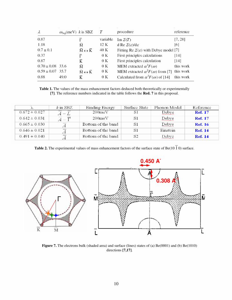
For Be(0001), several papers reported the mass enhancement factors of its surface state [7-13]. However, the values of the enhancement factors are not consistent to each other. The values are listed in Table 1., range from 0.37 to 1.18. It is worthy to mention that the data were taken from different positions in the reciprocal space, indicated as symbols, Γ , K , M and M �K , as shown in Fig. 7 (a). One thing needs to be careful

8

Figure 5. The real space structure (c) and reciprocal space structures (b) of beryllium. In 2D Be

surfaces, (a) is Be(0001) and (d) is Be(10 1 0) surfaces [44-45]. (a)

(b)

Figure 6. The electron structures of bulk beryllium and (a) Be(0001) [46] and (b)

Be(10 1 0) [16] in some main directions in the reciprocal space.

(b)

(c)

(d)

(a)

9

concerned is that the meaning of “ M ”, “ K ” or “ M �K ” are referring to the points, indicated in Fig. 7 (a) with blue, orange and green stars, where the surface state, centered at Γ , meets the Fermi energy along the indicated directions, not really lie on the M , K or M �K points in reciprocal lattice. The Fermi momentum of the highly symmetric surface state centered at Γ of the Be(0001) surface is about 0.947 Å-1 [7]. The possible reason for this situation of the inconsistency of the mass enhancement factors might be the mass enhancement factors are dependent on the position in the reciprocal space.

For the Be(10 1 0) surface, the Fermi surface with the indication of the bulk state and the surface states are shown in Fig. 7 (b). The surface state centered at A has an eccentricity � = 0.684, with the Fermi momentum of 0.450 Å-1 and 0.308 Å-1 along

LA − and Γ−A directions, respectively [17]. The values of the mass enhancement factors are list in table 2 [14, 16-17]. In table 2, the S1 and S2 indicate the surface states centered at A with different binding energies, see Fig. 6 (b). S1 denotes the higher energy surface state which crosses the Fermi energy; S2 denotes the lower energy surface state. All the values in table 2 were obtained by the method of fitting the temperature-dependent imaginary part of the self energy with eq. (7) with either Debye phonon model or Einstein phonon model. The values seems consistent with each other, however, more experimental data is needed to confirm this conclusion.

In order to understand more about the electron-phonon interaction, the hydrogen is always used to be adsorbed on the beryllium surface. The theoretical researches [25-34] for the modified beryllium surfaces are much more than the experimental researches [22-25, 54-56]. However, only three papers reported the photoemission study of the modified beryllium surface. One of them studied the hydrogen modified Be(0001) surface [22], while the other two studied the lithium modified Be surfaces [54-55]. According to the ref. 23, the adsorbed hydrogen favors the bridge sites and would change the work function about -0.5 eV when the coverage of the bridge site saturates. From the photoemission study of the hydrogen modified Be(0001) surface [22], the clean beryllium surface state centered at Γ (band width is about 2.78 eV) is broaden as increasing the covering hydrogen and vanished when the covering hydrogen reach 5L (L= Torr · s). At this coverage of hydrogen, there are two new surface states appeared with the binding energies are equal to about 4.2 eV and 10.2 eV at Γ point, as shown in fig. 8. The effective mass of the band, with binding energy of about 4.2 eV, located at Γ , were also measured as 0.88 and 0.90 along the K−Γ and the M−Γ directions, respectively; while the effective mass of the other band, with the binding energy of about 10.2 eV, located at Γ , was measured as 1.5, and the effective mass of the band located at M was measured as 0.23 along the Γ−M direction. However, there is no report related to the measurement of mass enhancement factors of these states of hydrogen modified beryllium surfaces.

There are some papers related to the measurement of the phonon dispersions [36, 38-39]. The bulk phonon dispersions were measured by Stedman et. al., as shown in Fig. 9 (a) [55]. The points in the reciprocal lattice of hcp are indicated in Fig. 9 (b) [38]. The surface phonon dispersions of Be(0001) and Be(10 1 0) surfaces were measured by HREELS [36, 39]. The surface phonon dispersion of Be(0001) along the high symmetry directions, as shown in Fig. 9(c), has a strong peak in HREELS and three more weak peaks. The strong peaks were indicated as filled circles, while the weak peaks were

10

Table 1. The values of the mass enhancement factors deduced both theoretically or experimentally [7]. The reference numbers indicated in the table follows the Red. 7 in this proposal.

Table 2. The experimental values of mass enhancement factors of the surface state of Be(10 1 0) surface.

0.450 A-

1

0.308 A-1

�

Figure 7. The electrons bulk (shaded area) and surface (lines) states of (a) Be(0001) and (b) Be(1010) directions [7,17].

11

Figure 8. The electron structures of the bulk beryllium (shadowed area) and Be(0001) surface

(open circles) and the hydrogen modified Be(0001) surface (filled circles) [22].

indicated as open circles in the figure. The surface phonon dispersion of Be(10 1 0) surface were also measured and shown in Fig. 9 (d). The phonon dispersion of Be(10 1 0) surface does not disperse too much. Although the phonon dispersions of clean beryllium surfaces were measured, there is no report related to the phonon dispersion of hydrogen modified beryllium surface.

Research methods; current progress and future plans: As mentioned above, the goal of this proposal is to understand more about the

mechanism of EPC by means of determining the mass enhancement factors at different points in reciprocal space on four kinds of beryllium surfaces by using ARPES. The different directions can be found in Fig. 7 in both Be(0001) or Be(10 1 0) surfaces; while the four kinds of beryllium surfaces are: clean Be(0001); clean Be(10 1 0); hydrogen modified Be(0001); hydrogen modified Be(10 1 0) surfaces.

The first experiment of this work was already performed at ASTRID (Aarhus Storage Ring in Denmark), Denmark in April 2005. In this measurement, the data of surface states of clean Be(0001) along some high symmetric directions were collected. The procedure of the experiment was: clean the surface of Be(0001) by using Ar ion gun sputtering at 450 °C in 5 minutes and followed by an annealing at 550°C in 15 minutes, and repeated two more cycles. Then use Auger electron spectroscopy (AES) to make sure the surface was clean. After the preparation procedure, as described above, the sample was sent to ARPES chamber to take the ARPES data with different temperature range from 50K to 650K with 100K difference per step.

Figure 10 shows the ARPES data of the surface state centered at Γ of the clean Be(0001) surface measured at ASTRID, Denmark. After the fitting and the analysis, the imaginary part of the electron self energy as a function of binding energy were extracted, as shown in fig. 11. In fig. 11, three kinds of approaches were used: Linear (green squares), Semi-Linear (red squares) and quadratic (black squares). The linear approach was described previously, which uses the linear dispersion for the bare energy dispersion relation in the spectral function (eq. 13) and uses eq. 15 to extract the

12

Figure 9. Phonon dispersions of (a) bulk beryllium [38]; (c) Be(0001) surface [36] and (d)

Be(10 1 0) surface [39]. The points in reciprocal space can be found in (b) [38].

(a) (b)

(c) (d)

Figure 10. The ARPES data of the surface state centered at Γ of the clean Be(0001) surface measured at ASTRID, Denmark.

13

0.0 0.5 1.0 1.5 2.0

0.24

0.30

0.36

Quadratic Linear Semi-Linear

ImΣΣ ΣΣ (

eV)

Binding Energy (eV)

50K(a)

0.0 0.5 1.0 1.5 2.0 2.5

0.2

0.3

0.4

0.5

Quadratic Linear Semi-Linear

650K

ImΣΣ ΣΣ(

eV)

Binding Energy (eV)

(b)

Figure 11. The imaginary part of the electron self energy with temperature as (a) 50 K and (b) 650 K by using three kinds of approaches: Linear (green squares); Semi-Linear (red squares) and

Quadratic (black squares).

imaginary part of the self energy. The semi-linear approach uses the same energy dispersion relation (linear relation) in the spectral function as well. The difference is that the equation relates the imaginary part of the self energy to the FWHM of the MDCs as follows [43]:

( ) ( ) ( ) ( )ωωωωω 222

02Im WkW

k mF

−=Σ (16)

the idea for eq. 16 is based on the quadratic dispersion relation. Both of above two approaches are used widely but have problems when dealing with the data near the bottom of the band. Near the bottom of the band, the local velocity v will approach to zero in eq. 15, which will cause the imaginary part of the self energy to be zero; the momentum k will approach to zero in eq. 16, which will cause the number in the square root to be negative. Here, we proposed a new approach, the quadratic approach. The quadratic approach uses the quadratic energy dispersion relation function in the spectral function. Then the spectral function can be written as:

( )( )

( ) ( ) 2

2

2

222

2

2

ImRe

Im,

��

���

� Σ+��

���

� Σ−+−

���

�Σ

∝

Fb

Fb

F

F

b

kE

kE

kk

kE

kAωωω

ωω

� (17)

If the ARPES data is plot as a function of k2 with a constant energy, the special MDCs (hereafter denote as MDCs*) can be fit as a symmetric Lorentzian function. The imaginary part of the self energy relates to the FWHM of MDCs* could be written as:

( ) ( )b

F

EkMDCsFWHM

22*

Im =Σ ω (18)

By using this approach, the problem occurred in previous two approaches when dealing with the data near the bottom of the band can be solved. It is clearly to see in Fig. 11, the imaginary part of the electron self energy are similar when the binding energy smaller

14

than about 1.9 eV among these three kinds of approaches, except for a little vertical shifting. However, when the binding energy is larger than about 1.9 eV, the trend of the imaginary part of the electron self energy went to different way between quadratic and linear/semi-linear approaches. In both Fig. 11 (a) and (b), which are the data taken when the temperatures were at 50 K and 650 K, respectively, the imaginary part of the electron self energy extracted both by Linear or Semi-Linear go toward to zero when the binding energy getting higher while the imaginary part of the electron self energy extracted by Quadratic approach goes up.

There is a new ARPES system is being built in UT currently. The detector is SCIENTA R4000, made by a Sweden company, Gammadata. The energy resolution could be less than 1 meV; The ultimate angular resolution could be less than 0.1 degree; The spatial resolution could be less than 9 �m.

Synchrotron will be used to measure the Be(0001) and hydrogen modified Be(0001) surfaces. The proposal to use the beam time in ALS (advanced light source) is approved. ALS is located at Berkeley, CA, and has been completely constructed since 1993. The facility operates with electrons with a nominal energy of 1.9 GeV in the storage ring. The size of the electron beam in the storage ring is about 0.20 mm × 0.02 mm. The number of the operating beam lines is about 35 plus the beam test facility, while the number of the possible beam lines could be 50.

The phonon dispersion is going to be examined by HREELS (high resolution electron energy loss spectroscopy) system. The HREELS system, which is rebuilt currently, is the VSW HIB1000 made by VSW Science Instruments. The surface orientation would be monitored by a LEED system.

Hopefully, I can learn many things when involved in doing the research of the electron phonon interaction on the beryllium surfaces and then be able to graduate. Of course, the results of this study would be helpful to understand many-body interacting phenomenon. References:

1. J. Bardeen, L. N. Cooper, and J. R. Schrieffer, Phys. Rev. 108, 1175(1957). 2. J. Bardeen, L. N. Cooper, and J. R. Schrieffer, Phys. Rev. 106, 162(1957). 3. L. N. Cooper, Phys. Rev. 104, 1189(1956). 4. G. M. Eliashberg, Soviet Phys. JETP 11, 696(1960). 5. G. Grimvall, The Electron-Phonon Interaction in Metals, Selected Topics in Solid

State Physics, edited by E. Wohlfarth (North-Holland, New York, 1981). 6. G. D. Mahan, Many-Particle Physics, Physics of solidsand liquids, (Kluwer

Academic/Plenum Publishers, New York, 2000). 7. S.-J. Tang, J. Shi, B. Wu, P. T. Sprunger, W. L. Yang, V. Brouet, X. J. Zhou, Z.

Hussain, Z.-X. Shen, Z. Zhang, and E. W. Plummer, Phys. Stat. Sol. (b) 241, 2345(2004).

8. M. Hengsberger, D. Purdie, P. Segovia, and Y. Baer, Phys. Rev. Lett. 83, 592(1999).

9. M. Hengsberger, R. Fresard, D. Purdie, P. Segovia, and Y. Baer, Phys. Rev. B 60, 10796(1999).

10. S. LaShell, E. Jensen, and T. Balasubramanian, Phys. Rev. B 61, 2371(2000).

15

11. A. Eiguren, S. de Gironcoli, E. V. Chulkov, P. M. Echenique, and E. Tosatti, Phys. Rev. Lett. 91, 166803(2003).

12. E. V. Chulkov, V. M. Silkin, and E. N. Shirykalov, Surf. Sci. 188, 287(1987). 13. T. Balasubramanian, and E. Jensen, Phys. Rev. B 57, R6866(1998). 14. S.-J. Tang, Ismail, P. T. Sprunger, and E. W. Plummer, Phys. Rev. B 65,

235428(2002). 15. J. Shi, S.-J. Tang, B. Wu, P. T. Sprunger, W. L. Yang, V. Brouet, X. J. Zhou, Z.

Hussain, Z.-X. Shen, Z. Zhang, and E. W. Plummer, Phys. Rev. Lett. 92, 186401(2004).

16. T. Balasubramanian, L. I. Johansson, P.-A. Glans, C. Virojanadara, V. M. Silkin, E. V. Chulkov, and P. M. Echenique, Phys. Rev. B 64, 205401(2001).

17. T. Balasubramanian, P.-A. Glans, and L. I. Johansson, Phys. Rev. B 61, 12709(2000).

18. B. G. Lazarev, E. E. Semenenko, and A. I. Sudowtsov, Sov. Phys. JETP 13, 75(1961).

19. N. E. Alekseevskii, and V. I. Tsebro, J. Low Temp. Phys. 4, 679(1971). 20. K. Takei, M. Okamoto, K. Nakanura, and Y. Maeda, Jpn. J. Appl. Phys., Part 1 26,

386(1987). 21. R. L. Falge Jr., Phys. Lett. 24A, 579(1967). 22. K. B. Ray, X. Pan, and E. W. Plummer, Surf. Sci. 285, 66(1993). 23. K. B. Ray, J. B. Hannon, and E. W. Plummer, Chem. Phys. Lett. 171, 469(1990). 24. G. S. Tompa, W. E. Carr, and M. Seidl, Surf. Sci. 198, 431(1988). 25. M. M. Marino, W. C. Ermler, G. S. Tompa, and M. Seidl, Surf. Sci. 208,

189(1989). 26. J. Z. Wu, S. B. Trickey, and J. C. Boettger, Phys. Rev. B 42, 1668(1990). 27. P. S. Bagus, H. F. Schaefer III, and C. W. Bauschlicher, Jr., J. Chem. Phys. 78,

1390(1983). 28. J. W. Mintmire, J. R. Sabin, and S. B. Trickey, Phys. Rev. B 26, 1743(1982). 29. J. Rubio, F. Illas, and J. M. Ricart, J. Chem. Phys. 84, 3311(1986). 30. M. Seel, Phys. Rev. B 43, 9532(1991). 31. R. Yu, and P. K. Lam, Phys. Rev. B 39, 5035(1989). 32. B. N. Cox, and C. W. Bauschlicher, Jr., Surf. Sci. 102, 295(1981). 33. G. Angonoa, J. Koutecky, A. N. Ermoshkin, and C. Pisani, Surf. Sci. 138,

51(1984). 34. C. W. Bauschlicher, Jr., and P. S. Bagus, Chem. Phys. Lett. 90, 355(1982). 35. J. B. Hannon, and E. W. Plummer, J. Electron Spectros. Rel. Phenom. 64/65,

683(1993). 36. J. B. Hannon, E. J. Mele, and E. W. Plummer, Phys. Rev. B 53, 2090(1996). 37. E. W. Plummer, and J. B. Hannon, Prog. Surf. Sci. 46, 149(1994). 38. R. Stedman, Z. Amilius, R. Pauli, and O. Sundin, J. Phys. F: Metal Phys. 6,

157(1976). 39. P. Hofmann, and E. W. Plummer, Surf. Sci. 377-379, 330(1997). 40. H. Fröhlich, Phys. Rev. 79, 845(1950). 41. F. Reinert, and S. Hüfner, New J. Phys. 7, 97(2005). 42. A. Damascelli, Phys. Scrip. T109, 61(2004).

16

43. A. A. Kordyuk, S. V. Borisenko, A. Koitzsch, J. Fink, M. Knupfer, and H. Berger, Phys. Rev. B 71, 214513(2005).

44. E. Jensen, R. A. Bartynski, T. Gustafsson, E. W. Plummer, M. Y. Chou, M. L. Cohen, and G. B. Hoflund, Phys. Rev. B 30, 5500(1984).

45. P. Hofmann, R. Stumpf, V. M. Silkin, E. V. Chulkov, and E. W. Plummer, Surf. Sci. 355, L278(1996).

46. R. A. Bartynski, E. Jensen, T. Gustafsson, and E. W. Plummer, Phys. Rev. B 32, 1921(1985).

47. Ismail, P. Hofmann, A. P. Baddorf, and E. W. Plummer, Phys. Rev. B 66, 245414(2002).

48. P.-A. Glans, L. I. Johansson, T. Balasubramanian, and R. J. Blake, Phys. Rev. B 70, 033408(2004).

49. L. I. Johansson, and B. E. Sernelius, Phys. Rev. B 50, 16817(1994). 50. J. C. Boettger, and S. B. Trickey, Phys. Rev. B 34, 3604(1986). 51. L. I. Johansson, H. I. P. Johansson, J. N. Andersen, E. Lundgren, and R. Nyholm,

Phys. Rev. Lett. 71, 2453(1993). 52. U. O. Karlsson, S. A. Flodström, R. Engelhardt, W. Gädeke, and E. E. Koch,

Solid State Comm. 49, 711(1984). 53. V. M. Silkin, T. Balasubramanian, E. V. Chulkov, A. Rubio, and P. M. Echenique,

Phys. Rev. B 64, 085334(2001). 54. G. M. Watson, P. A. Bruhwiler, E. W. Plummer, H.-J. Sagner, and K.-H. Frank,

Phys. Rev. Lett. 65, 468(1990). 55. L. I. Johansson, T. Balasubramanian, and C. Virojanadara, Surf. Rev. Lett. 9,

1493(2002). 56. G. S. Tompa, M. Seidl, W. C. Ermler, and W. E. Carr, Surf. Sci. 185, L453(1987).