6/7/2012

1

Electron Focusing Through a Magnetic Lens

© 2012 COMSOL. COMSOL and COMSOL Multiphysics are registered trademarks of COMSOL AB. Capture the Concept, COMSOL Desktop, and LiveLink are trademarks of COMSOL AB. Other product or brand names are trademarks or registered trademarks of their respective holders.

John Dunec, Ph.D.

VP of Sales, NW USA

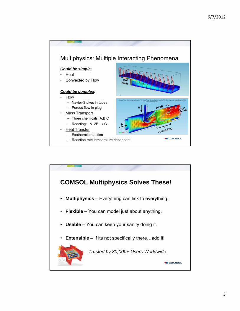
Welcome to the Lunch-Time Tutorials!

• Solve One Problem Using COMSOL Multiphysics

This Tutorial: Electron Focusing Through a Magnetic Lens• This Tutorial: Electron Focusing Through a Magnetic Lens

• 30-35 minutes duration

• Short Q&A at end

• Archived at:

www.comsol.com/webinars

Upcoming Tutorials:

• Magnetophoretic cell separation

www.comsol.com/events

Presentation, Step-by-Steps, and COMSOL model available on request

6/7/2012

2

Individual Physics you Learned in School

Heat in a rod, … S i h

• Individual equation sets … Applied to simple, (and sometimes not-so-simple) single-physics problems

Stress in a wrench

In Reality – Multiple Sets of Physics Interact

• Typically bi-directional nonlinear coupling between multiple physical processes

6/7/2012

3

Multiphysics: Multiple Interacting Phenomena

Could be simple:

• HeatHeat

• Convected by Flow

Could be complex:

• Flow– Navier-Stokes in tubes

– Porous flow in plug B

• Mass Transport– Three chemicals: A,B,C

– Reacting: A+2B → C

• Heat Transfer– Exothermic reaction

– Reaction rate temperature dependant

COMSOL Multiphysics Solves These!

• Multiphysics – Everything can link to everything.Multiphysics Everything can link to everything.

• Flexible – You can model just about anything.

• Usable – You can keep your sanity doing it.

• Extensible – If its not specifically there…add it!

Trusted by 80,000+ Users Worldwide

6/7/2012

4

Anywhere you can type a number …you can type an equation

• Or an interpolation function• Or an interpolation function …

• And it can depend on anything known in your problem

• Example: Concentration-dependant viscosity:

Low concentration, High velocity

221001.0 cHigh concentration, Low velocity

Electron Focusing Through a Magnetic Lens

Key Elements

Simulating a magnetic field from• Simulating a magnetic field from an electric coil

• Setting up a multi-turn coil in COMSOL

• Using Particle Tracing to plot trajectories of electrons responding to magnetic field

6/7/2012

5

Two Physics: Magnetics & Particle Tracing

Magnetics Particle Tracing

• Particles respond to Magnetic Forces

COMSOL Products Used – This Tutorial

AutoCAD® and Inventor® are registered trademarks of Autodesk, Inc. LiveLink™ for AutoCAD® and LiveLink™ for Inventor® are not affiliated with, endorsed by, sponsored by, or supported by Autodesk, Inc. and/or any of its affiliates and/or subsidiaries. CATIA® is a registered trademark of Dassault Systèmes S.A. or its affiliates or subsidiaries. SolidWorks® is a registered trademark of Dassault Systèmes SolidWorks Corporation or its parent, affiliates, or subsidiaries. Creo™ is a trademark and Pro/ENGINEER® is a registered trademark of Parametric Technology Corporation or its subsidiaries in the U.S and/or in other countries. MATLAB® is a registered trademark of The MathWorks, Inc.

• COMSOL Multiphysics, AC/DC Module

• Along with the Particle Tracing Module

6/7/2012

6

Tutorial Roadmap

First: Setup and Solve Magnetics Problem

Choose predefined multiphysics• Choose predefined multiphysics

• Import geometry sequence

• Define materials (Copper and Air)

• Set up Coil

• Mesh

• Solve

Next: Add Particle Tracing Magnetic Field Surrounding Multi-turn

Electric Coil

Geometry

• Air domain with

Magnetic In

electrons

• Copper mechanical structure

• Multi-turn electric coil

Coil

Copper

Copper

C

Air

nsulation on all Outerelectric coil

• Electron “Inlet” at bottom of bottom copper annulus

Copper

Electron “Inlet”

r Boundaries

6/7/2012

7

1st Solve for Magnetic Field

• Solve based on Magnetic Potential

• Ampere’s Law relates H and B

AB

JH

e

HB 0

• Applied Volumetric Current from a Multi-turn Coil

HB r0

coilareacrosswire

coile A

INeJ

Modeling Nuts & Bolts: Coil Ref Circle

We Need to Define a “Reference Edge”

• To Trace the Path of the Current and …

• To Determine the Average Coil Length

Draw a mid-coil circle on

top of actual coil domain

6/7/2012

8

Let’s do this in COMSOL …

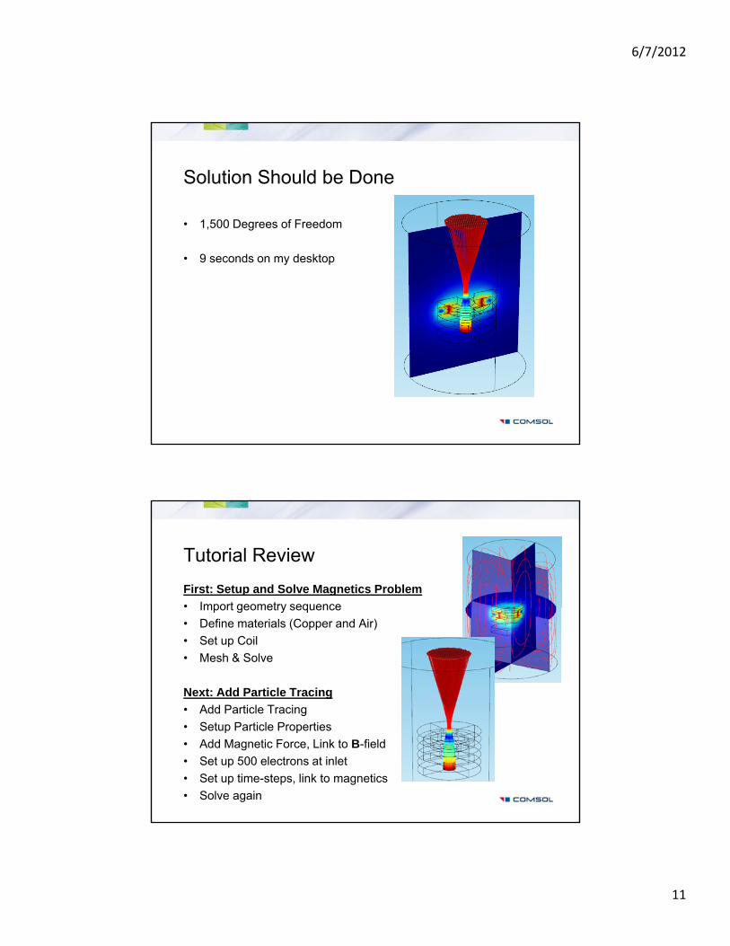
Solution Should be Done

• 175,000 Degrees of Freedomg

• 25 seconds on my desktop

6/7/2012

9

Next Add Particle Tracing for Electrons

Add 2nd Physics: y

• Particle Tracing, Transient

Define Particle Physics

• Define the Particle Properties

• Add the Magnetic Force, Link to B field

• Create an Inlet (500 electrons, velocity = 1.33e7)

Set up Transient Study

• Time Stepping

• Link Transient Particle Tracing to Magnetic Stationary Results

Lorenz Force on the Electrons

• Newton’s Law – recast to change in momentumg

• The force will be the Lorentz force of a particle in a magnetic field – which changes the momentum

vaF mdt

dm

• v is particle velocity vector, q is the particle charge, m is the particle mass

Bvv qmdt

d

6/7/2012

10

Magnetic Lens

• Solve for Magnetic Field from simple Coilp

• Apply Magnetic Force to electron particles entering from below

• Vector cross product with B-field causes particles to both spiral & focusfocus

B-Field Vectors

Bvv qmdt

d

Let’s do this in COMSOL …

6/7/2012

11

Solution Should be Done

• 1,500 Degrees of Freedomg

• 9 seconds on my desktop

Tutorial Review

First: Setup and Solve Magnetics Problem

• Import geometry sequenceImport geometry sequence

• Define materials (Copper and Air)

• Set up Coil

• Mesh & Solve

Next: Add Particle Tracing

• Add Particle Tracingg

• Setup Particle Properties

• Add Magnetic Force, Link to B-field

• Set up 500 electrons at inlet

• Set up time-steps, link to magnetics

• Solve again

6/7/2012

12

To Get More Information …

Attend a Free Seminar

• Includes 2-week trial of COMSOL

• www.comsol.com/events

Attend our Webinars

• www.comsol.com/events/webinars/

Contact Your Local COMSOL Office

• www.comsol.com/contact

Attend our Annual Conference

• www.comsol.com/conference2012

6/7/2012

13

www.comsol.com

6/7/2012

14

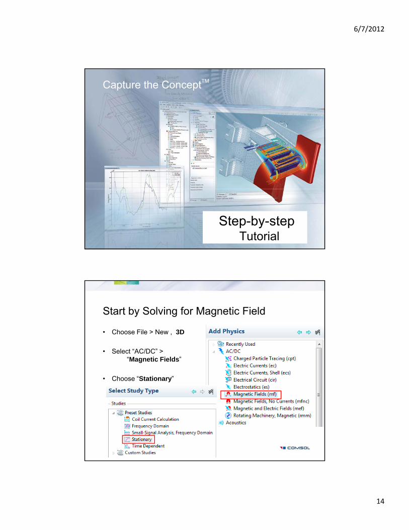
Capture the ConceptTM

Step-by-step Tutorial

Step-by-step Tutorial

Start by Solving for Magnetic Field

• Choose File > New , 3D

• Select “AC/DC” > “Magnetic Fields”

• Choose “Stationary”

6/7/2012

15

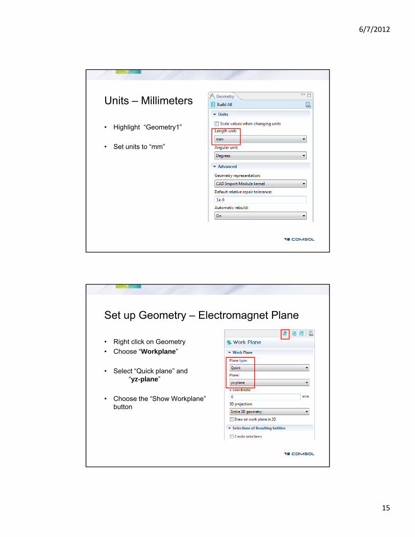
Units – Millimeters

• Highlight “Geometry1”g g y

• Set units to “mm”

Set up Geometry – Electromagnet Plane

• Right click on Geometry g y

• Choose “Workplane”

• Select “Quick plane” and “yz-plane”

• Choose the “Show Workplane” buttonbutton

6/7/2012

16

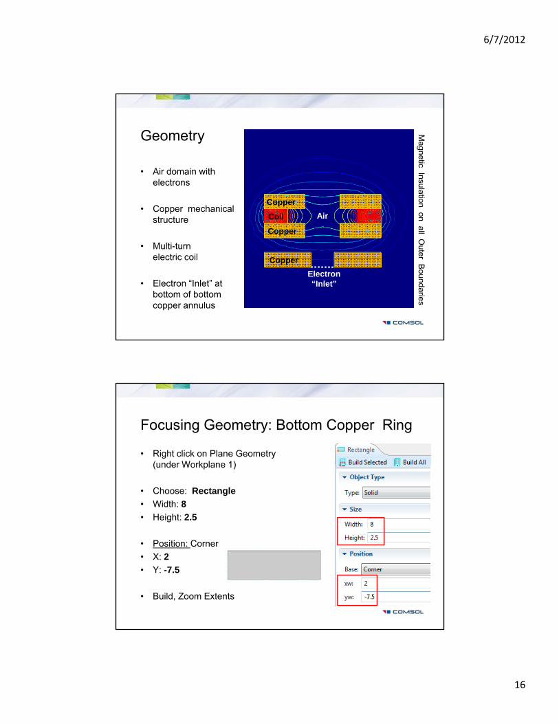
Geometry

• Air domain with

Magnetic In

electrons

• Copper mechanical structure

• Multi-turn electric coil

Coil

Copper

Copper

C

Air

nsulation on all Outerelectric coil

• Electron “Inlet” at bottom of bottom copper annulus

Copper

Electron “Inlet”

r Boundaries

Focusing Geometry: Bottom Copper Ring

• Right click on Plane Geometry (under Workplane 1)(under Workplane 1)

• Choose: Rectangle

• Width: 8

• Height: 2.5

• Position: Corner

• X: 2

• Y: -7.5

• Build, Zoom Extents

6/7/2012

17

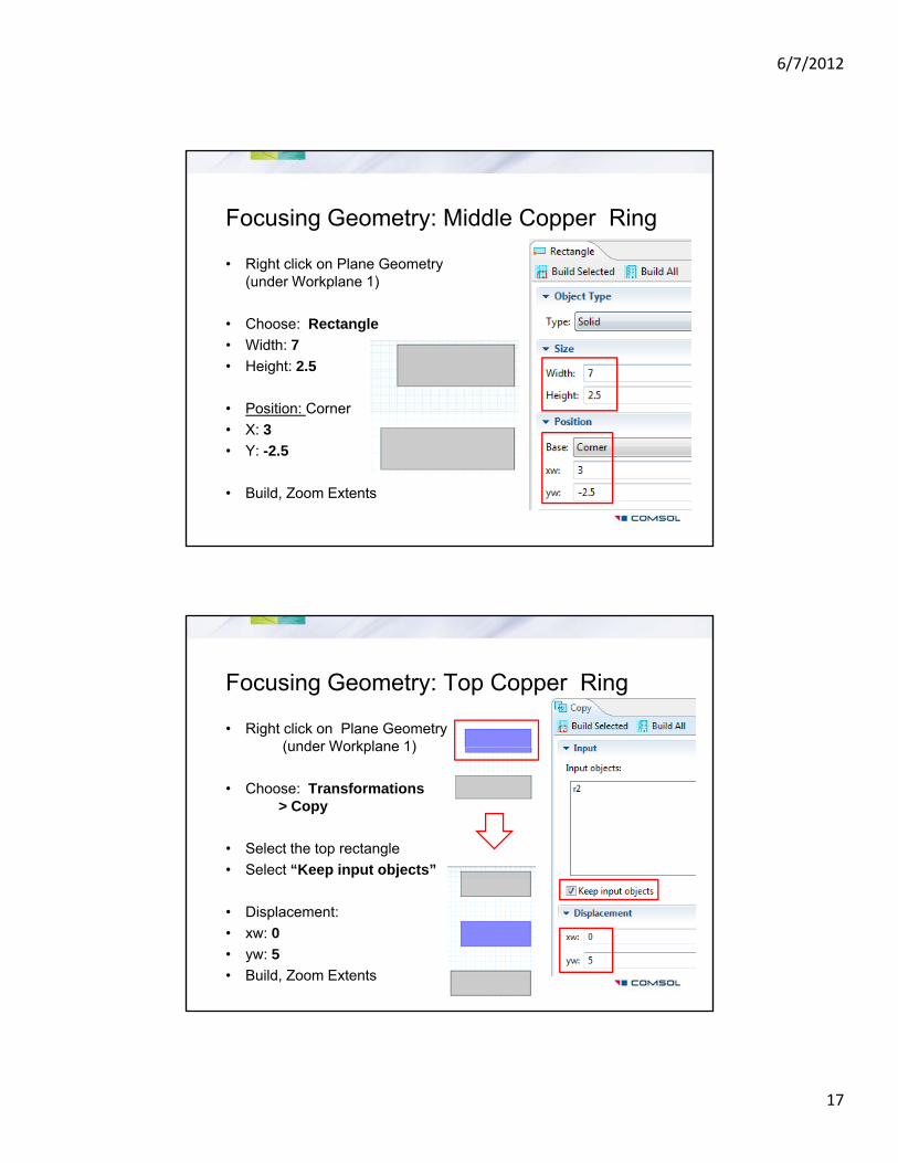
Focusing Geometry: Middle Copper Ring

• Right click on Plane Geometry (under Workplane 1)(under Workplane 1)

• Choose: Rectangle

• Width: 7

• Height: 2.5

• Position: Corner

• X: 3

• Y: -2.5

• Build, Zoom Extents

Focusing Geometry: Top Copper Ring

• Right click on Plane Geometry(under Workplane 1)(under Workplane 1)

• Choose: Transformations > Copy

• Select the top rectangle

• Select “Keep input objects”

• Displacement:

• xw: 0

• yw: 5

• Build, Zoom Extents

6/7/2012

18

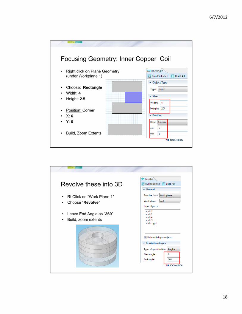
Focusing Geometry: Inner Copper Coil

• Right click on Plane Geometry (under Workplane 1)(under Workplane 1)

• Choose: Rectangle

• Width: 4

• Height: 2.5

• Position: Corner

• X: 6

• Y: 0

• Build, Zoom Extents

Revolve these into 3D

• Rt Click on “Work Plane 1”

Choose “Revolve”• Choose Revolve”

• Leave End Angle as “360”

• Build, zoom extents

6/7/2012

19

Draw the Electron Inlet Surface

• Rt Click on “Geometry 1”

Choose “Workplane”• Choose Workplane”

• Select “Face Parallel”

• Pick the bottom face of the copper

• Choose the “Show Workplane” Icon

• Choose “Zoom Extents”

• Pick the Draw centered circle” buttonPick the Draw centered circle button

• Draw a circle as shown

• (Line up with the inner circle)

• Build all

• Highlight “Geometry” > Build all

Geometry: Surrounding Air

• Rt click on “Geometry 1”y

• Select “Cylinder”

• Radius: 20

• Height: 50

• Position: z = -20

(Negative!)

6/7/2012

20

Materials

• Rt Click on “Materials”

• Choose “Material Browser”

• Expand “Built-in”

• Rt click on “Copper”

• Add material to Model

• Make sure “All domains” is selected

• Pick “Material Browser” tab

• Rt click on “Air”

• Add material to Model

• Select the outer Air Domain

Specify Coil Domain

• Rt Click on “Magnetic Fields”g

• Add “Multi turn Coil Domain”

• Select the 2nd Annulus from top

• Change “Coil Type” to “Circular”

• Enter Number of Turns as “1000”

• Coil Current as “0.32[A]”

6/7/2012

21

Reference Circle for Coil

We Need to Define a “Reference Edge”

To Trace the Path of the Current and• To Trace the Path of the Current and …

• To Determine the Average Coil Length

Draw a Mid-Coil Circle

• Rt Click on Geometry 1

• Choose “Workplane”

• “Quick Plane” “x-y” z-coord: “2 5”Quick Plane x y z coord: 2.5

• Choose “Show Workplane” > Zoom Extents

• Rt Click on “Plane Geometry”

• Choose “Circle”

• Radius 8 mm, Center on (0,0)

• Build all

Choose Circle as Reference Edge

• Rt Click on “Multi-Turn Coil Domain”

• Choose “Edges” > Reference Edge”

• Pick the Broom Icon to Clear the list

• Pick the mid-line circular edges just drawn on the top of the coil domain

6/7/2012

22

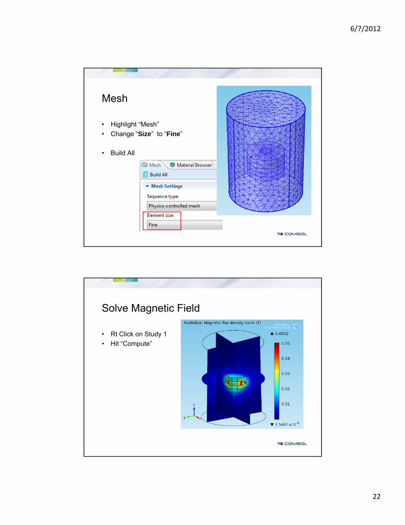
Mesh

• Highlight “Mesh”g g

• Change “Size” to “Fine”

• Build All

Solve Magnetic Field

• Rt Click on Study 1y

• Hit “Compute”

6/7/2012

23

Add Particle Tracing

• Rt click on “Model 1”

Choose “Add Physics”• Choose Add Physics”

• Choose “AC/DC” > “Charged Particle Tracing”

• Choose the blue “Next” arrow

• Choose “Time Dependant”p

• Deselect “Solve For” Magnetic Fields

• Pick Finish Flag

Note: You need an additional study since particle tracing is transient whereas the magnetic analysis was stationary.

Particles only in Air Domain

• Highlight “Charged Particle Tracing”

• Go to “Domain” section

• Pick “Clear Selection” button (the broom)

• Choose only Air domain, (domain #1)

6/7/2012

24

Add Lorenz Magnetic Force to Particles

• Rt Click on “Charged Particle Tracing”g g

• Choose “Magnetic Force”

• Select only the Air Domain (#1)

• Under Magnetic Force selection for B list

• Choose “Magnetic flux density mf/mf”

Note Particle Properties

• Under “Charged Particle Tracing”• Under Charged Particle Tracing

• Highlight “Particle Properties 1”

Leave as Default values:

• Particle mass: me constParticle mass: me_const(mass of an electron)

• Charge Number: -1

6/7/2012

25

BC: Particle Inlet

• Rt Click on “Charged Particle Tracing”

• Choose “Inlet”

• Select Indicated Boundary (#40)

• Choose “Projected Plane Grid

• Change “Initial position” to “Density”

• Set “N” to “500”• Set N to 500

Set Initial Velocity:

• 0 : x

• 0 : y

• 1.33e7[m/s] : z

Walls – Leave as “Freeze”

• Under “Charged Particle Tracing”g g

• Highlight “Wall 1”

• Leave “Wall Condition” as default “Freeze”

That way we can get statistics later

6/7/2012

26

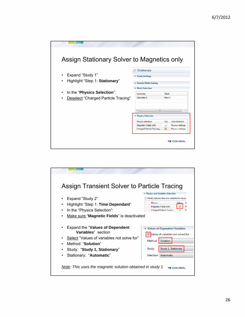
Assign Stationary Solver to Magnetics only

• Expand “Study 1”p y

• Highlight “Step 1: Stationary”

• In the “Physics Selection”:

• Deselect “Charged Particle Tracing”

Assign Transient Solver to Particle Tracing

• Expand “Study 2”

Highlight “Step 1: Time Dependant”• Highlight Step 1: Time Dependant”

• In the “Physics Selection”:

• Make sure “Magnetic Fields” is deactivated

• Expand the “Values of Dependent Variables” section

• Select “Values of variables not solve for”

• Method: “Solution”

• Study: “Study 1, Stationary”

• Stationary: “Automatic”

Note: This uses the magnetic solution obtained in study 1

6/7/2012

27

Set Times and Solve

• Highlight “Step 1: Time Dependant”

• Choose the “Range” button

• Set to “Number of Values”

• Start: “0”

• Stop: “5e-9”

• Number of Values: “25”

• Rt Click on Study 2 > Hit Compute

Add Lines to Trajectories

• Expand Particle Trajectories (cpt)

• Highlight “Particle Trajectories 1”

• Change “Type” to “Line”

• Plot

6/7/2012

28

Add Slice Plot of B-Field

• Rt Click on “Particle Tracing”

• Choose “Slice Plot”

Change to

• Plane Type: Quick

• Plane: zx-plane

Pl 1• Planes: 1

• Leave default expression: mf.normB (magnetic flux density)

www.comsol.com