Embed Size (px)
Citation preview

Electromechanical Modeling and Simulation of Thin
Cardiac Tissue Constructs –
Smoothed FEM Applied to a Biomechanical Plate Problem
Von der Fakultat fur Ingenieurwissenschaften,Abteilung Bauwissenschaftender Universitat Duisburg-Essen
zur Erlangung des akademischen Grades
Doktor-Ingenieur
genehmigte Dissertation
von
Ralf Frotscher, M.Sc.
Hauptberichter: Prof. Dr.-Ing. habil. J. SchroderBetreuer: Prof. Dr.-Ing. M. StaatKorreferent: Prof. Dr.-Ing. W. Kowalczyk
Tag der Einreichung: 14. September 2015Tag der mundlichen Prufung: 16. Februar 2016
Fakultat fur Ingenieurwissenschaften,Abteilung Bauwissenschaftender Universitat Duisburg-Essen
Institut fur MechanikProf. Dr.-Ing. habil. J. Schroder

Herausgeber:
Prof. Dr.-Ing. habil. J. Schroder
Organisation und Verwaltung:
Prof. Dr.-Ing. habil. J. SchroderInstitut fur MechanikFakultat fur IngenieurwissenschaftenAbteilung BauwissenschaftenUniversitat Duisburg-EssenUniversitatsstraße 1545141 EssenTel.: 0201 / 183 - 2682Fax.: 0201 / 183 - 2680
© Ralf FrotscherLabor BiomechanikInstitut fur BioengineeringFachhochschule AachenHeinrich-Mußmann-Straße 152428 Julich
Alle Rechte, insbesondere das der Ubersetzung in fremde Sprachen, vorbehalten. OhneGenehmigung des Autors ist es nicht gestattet, dieses Heft ganz oder teilweise auffotomechanischem Wege (Fotokopie, Mikrokopie), elektronischem oder sonstigen Wegenzu vervielfaltigen.

Preface
The work on this thesis has been carried out under the supervision of Prof. Dr.-Ing.Manfred Staat at the Biomechanics Lab at Aachen University of Applied Sciences (FHAachen) in Julich where I started working in September 2010, in cooperation with Prof.Dr.-Ing. habil. Jorg Schroder, the director of the Institute for Mechanics at the UniversityDuisburg-Essen.
My work has been financially supported by
the ZIM cooperative project ”Einstellbares alloplastisches Schlingensystem zur min-imalinvasiven Therapie der Belastungsinkontinenz bei Frauen” (2010–2011) fundedby the German Federal Ministry of Economics and Technology (BMWi),
the project ”Cardiakytos: Messung mechanischer Grundspannungen und Schlagam-plituden von Monolayern stammzellbasierter Kardiomyozyten fur die funktionelleMedikamenten- und Toxinforschung” (2011–2013) that has been selected from theoperational program for NRW in ’Ziel 2: Regionale Wettbewerbsfahigkeit undBeschaftigung’ (2007–2013) which is co-financed by EFRE,
the project ”Optimierung des Systems Netzimplantat-Beckenboden zur therapeutis-chen Gewebeverstarkung nach der Integraltheorie” (2013–2015) funded by the Ger-man Federal Ministry of Education and Research and
the project ”CardiacDrums: Messung mechanischer Grundspannungen undSchlagamplituden von hiPS-basierten Kardiomyozyten fur funktionelleMedikamenten- und Toxintests in der personalisierten Medizin” (2014–2015)funded by funded by the German Ministry of Innovation, Science and Research(MIWF) through the program Translational Stem Cell Research.
My first and deep thankful thoughts are dedicated to Prof. Dr.-Ing. Manfred Staat whoguided me through this thesis and who taught me scientific working. His invaluable per-sonal and professional support was accompanied by introducing me into the field of Com-putational Biomechanics, by letting me develop my own scientific interests, by giving methe freedom to gain a broad and deep knowledge in different fields, by patience and byflexibility.
I want to thank Prof. Dr.-Ing. habil. Jorg Schroder for providing me the chance to obtaina PhD degree at his institute in terms of this cooperation and for his valuable commentson my mork.
Dr.-Ing. Minh Tuan Duong, who recently obtained his PhD degree at RWTH Aachen,I want to thank for his kindness and for the countless interesting, engaged, detailed,critical and thoughtful discussions through five years. I also thank Dr.-Ing. Thanh NgocTran who introduced me into the smoothed FEM and Karl-Heinz Gatzweiler for theintroduction in practical FEA and his technical support. The researchers at the Lab

4
of Medical and Molecular Biology helped me understanding cellular electrophysiologyand how cells behave in a tissue. Dr. rer. nat. Matthias Goßmann performed all theexperiments that are computationally investigated in here and I deeply appreciate hispatience in explaining his work to me. Dr.-Ing. Dominik Brands and Dr.-Ing. AlexanderSchwarz were very courteous in supporting my PhD project administratively and withregard to contents, respectively.
Special thanks to all the scientists I was able to meet at conferences and summer schoolsin Graz, Barcelona, Vienna, Minsk, Paris, Pavia and Aachen and to the graduate pro-gram of FH Aachen that financially supported some of these visits. These opportunitiesto personally discuss own and others work and to learn from experienced and leadingresearchers were precious.
I also want to thank my family who always encouraged me in continuing my academiccareer, my dear colleagues at FH Aachen and my Volleyball team for talking with meabout anything but my work.
The final paragraph is short because I do not have words to express the love and gratitudeI feel for my wife and daughters. Luckily I am able to show both everyday.
Leinfelden-Echterdingen, in February 2016 Ralf Frotscher
Abstract
This work models and simulates an inflation test for in vitro cardiac tissues in the frame-work of the Finite Element Method (FEM). It focuses on the simulation of drug treat-ment of autonomously beating cardiac tissue consisting of human-induced pluripotentstem cell-derived cardiac myocytes and the validation based on in-house experimental re-sults and on literature data. The ultra-thin composite material is modeled as a shell thatis coupled with Hodgkin-Huxley based systems of differential equations describing thecellular electrophysiology. Additionally, the edge-based smoothed FEM is investigatedconcerning its applicability to biomechanical plate problems. This method achieves ahigher accuracy than the standard FEM by smoothing the element-wise constant com-patible strains over the edges of the finite element mesh. It is especially beneficial in thecomputation of strongly distorted elements that are often created by automatic meshingof anatomical structures.The thesis starts by introducing the employed plate and FE theories, the electromechani-cal basics of cardiac tissue as well as of drug treatment and corresponding computationalmodels. The model is then applied to the inflation test that serves as the validation basisfor the quality and the ability of the model to predict drug effects on cardiac tissue.
Zusammenfassung
In dieser Arbeit wird ein Aufblasversuch fur in vitro Herzgewebe im Rahmen der Fi-nite Elemente Methode (FEM) modelliert und simuliert. Ziel ist dabei insbesondere dieSimulation von Medikamentenwirkung auf auto-kontraktile Herzgewebe bestehend ausvon human-induzierten pluripotenten Stammzellen abgeleiteten Kardiomyozyten undder Abgleich mit hausinternen experimentellen Resultaten und mit Literaturdaten. Furdas sehr dunne Kompositmaterial wird ein Schalenmodell aufgestellt und mit Hodgkin-Huxley basierten Differentialgleichungssystemen gekoppelt, die die zellulare Elektro-physiologie beschreiben. Zusatzlich wird die kanten-basiert geglattete FEM auf ihre An-wendbarkeit auf biomechanische Schalenprobleme hin untersucht. Diese Methode glattetdie elementweise konstanten, kompatiblen Dehnungen uber Elementgrenzen hinweg underreicht so eine hohere Genauigkeit, als die Standard FEM. Daruberhinaus eignet siesich in besonderem Maße fur die Berechnung auf stark verzerrten Elementen, die beiautomatischer Netzgenerierung fur anatomische Strukturen haufig entstehen.Zunachst werden die verwendeten Schalen- und FE-Theorien, die elektromechanischenGrundlagen von Herzgeweben, sowie von Medikamentenwirkung und einschlagige Mo-delle vorgestellt. Im Anschluß wird das Modell auf den Aufblasversuch angewandt, andem die Qualitat und die Fahigkeit des Modells Medikamentenwirkung auf Herzgewebevorherzusagen, validiert und beurteilt werden.


7
AbbreviationsCE contractile elementCM cardiomyocyteDSG Discrete Shear GapECM extracellular matrixhiPSC human-induced pluripotent stem cellhePSC human embryonic pluripotent stem cellhiPSC-CM human-induced pluripotent stem cell-derived cardiomyocyteFEM Finite Element MethodHMT Hunter-McCulloch-ter Keurs (model)MNT McAllister-Noble-Tsien (model)NHS Niederer-Hunter-Smith (model)ODE ordinary differential equationPE parallel elementQ4 4-noded quadrilateral (element)SE series elementS-FEM Smoothed Finite Element MethodTnC troponin CTT ten Tusscher (model)T3, T4, T6, T7 3-, 4-, 6-, 7-noded triangular (element)


9
Important symbols and notation
Indices
i ∈ 1, 2, 3α ∈ 1, 2I ∈ N0
Continuum Mechanicsei, ei global coordinate vectors and componentsξi, ξi local coordinate vectors and componentsX = (X1, X2, X3)
T position vector in reference configurationx = (x1, x2, x3)
T position vector in current configurationN0 normal vector in reference configurationn normal vector in current configurationθi contravariant curvilinear coordinatesd shell unit director in current configurationh shell thickness in current configurationu total displacementv displacement of shell middle planew change of shell directorθα rotation about α-axisχ change in thickness
(·)i,j =∂(·)i∂(·)j
derivative of component i with respect to coordinate j
(·),j directional derivativeI identityH displacement gradientF deformation gradientC right Cauchy-Green tensorb left Cauchy-Green tensorE Green-Lagrangian straine Euler-Almansi strainε strainεm shell membrane strainεl linear shell membrane strainεnl non-linear shell membrane strainεb shell bending strainεs shell transverse shear strainγ12, γ13, γ23 shear strain componentsσ Cauchy stressP 1st Piola-Kirchhoff stressS 2nd Piola-Kirchhoff stressN in-plane stress resultantsM bending momentsQ transverse forces

10
Constitutive equations
Ψ strain energyII scalar invariantλ, λi principal stretchesE Young’s modulusν poisson ratioCIJ Ogden material parametersp hydrostatic pressureC constitutive tensor
FEMΩ computational domainΓ boundary of the computational domainΓu,Γd Dirichlet (displacement) and Neumann (traction) boundary, respectively(·) quantity expressed in context-related coordinates
(·) quantity expressed in global coordinates
(·) quantity expressed in element coordinates(·) quantity expressed in smoothing domain coordinatesΩe
I domain occupied by element IΩs
I domain occupied by smoothing domain IΦ matrix of shape functionsΦenh matrix of enhanced shape functionsL1,L2 helper matricesB strain-displacement matrixKt tangent stiffness matrixK material stiffness matrixG geometrical stiffness matrixC material matrixu global displacement vectord local displacement vectorf internal force vectorNN total number of nodes in meshNe total number of elements in meshNs total number of smoothing domains in meshNn number of nodes of a smoothing domain or an element (from context)Bi
∗local strain-displacement matrix of domain Ωi related to a certain kind of strain
Rα∗I rotation matrix
Electrophysiology
Vm membrane action potentialI∗ ionic currentg∗ ionic gateIC50 half-inhibitory constant
Table of Contents I
Contents
1 Introduction 1
2 Continuum Mechanics and FEM 5
2.1 Continuum Mechanics . . . . . . . . . . . . . . . . . . . . . . . . . . . . . 5
2.1.1 Strain . . . . . . . . . . . . . . . . . . . . . . . . . . . . . . . . . . 6
2.1.2 Stress . . . . . . . . . . . . . . . . . . . . . . . . . . . . . . . . . . 7
2.2 Plate and Shell Theories . . . . . . . . . . . . . . . . . . . . . . . . . . . . 8
2.2.1 Plate Models . . . . . . . . . . . . . . . . . . . . . . . . . . . . . . 9
2.2.2 Reissner-Mindlin Plates in Detail . . . . . . . . . . . . . . . . . . . 10
2.3 Finite Element Method . . . . . . . . . . . . . . . . . . . . . . . . . . . . . 11
2.3.1 The Principle of Virtual Displacements . . . . . . . . . . . . . . . . 12
2.3.2 Variational Formulation . . . . . . . . . . . . . . . . . . . . . . . . 13
2.3.3 Discretization . . . . . . . . . . . . . . . . . . . . . . . . . . . . . . 13
2.3.4 Special Principles of Potential Energy . . . . . . . . . . . . . . . . . 15
2.3.4.1 Hu-Washizu . . . . . . . . . . . . . . . . . . . . . . . . . . 16
2.3.4.2 de Veubeke . . . . . . . . . . . . . . . . . . . . . . . . . . 16
2.3.5 Nonlinear FEM . . . . . . . . . . . . . . . . . . . . . . . . . . . . . 16
2.3.6 Finite Element Discretization of Plates and Shells . . . . . . . . . . 18
3 Smoothed FEM 19
3.1 Strain Smoothing . . . . . . . . . . . . . . . . . . . . . . . . . . . . . . . . 20
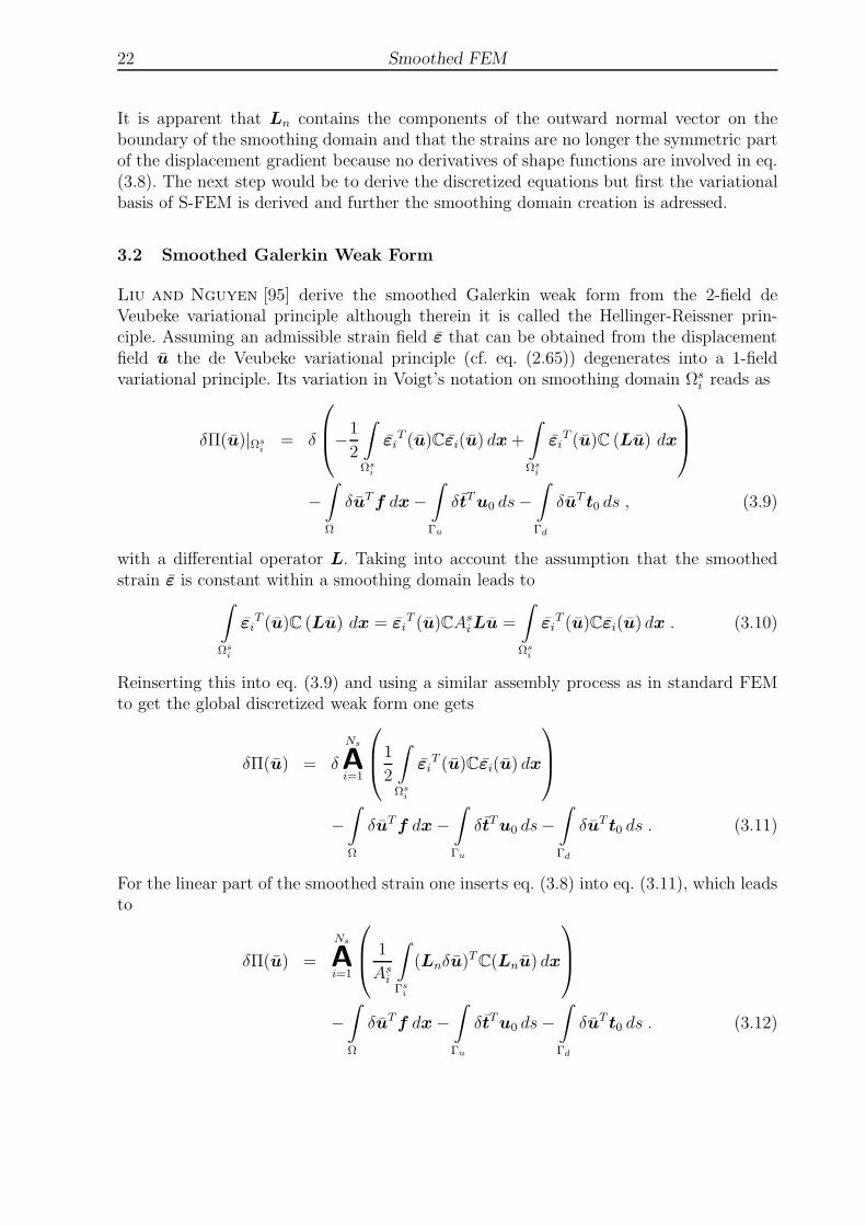
3.2 Smoothed Galerkin Weak Form . . . . . . . . . . . . . . . . . . . . . . . . 22
3.3 Smoothing Domains . . . . . . . . . . . . . . . . . . . . . . . . . . . . . . 23
3.4 Edge-based S-FEM for Nonlinear Plate Problems . . . . . . . . . . . . . . 24
3.5 Involving the Discrete Shear Gap Method . . . . . . . . . . . . . . . . . . 29
4 Cardiac Cells and Tissue 31
4.1 Purkinje Cells . . . . . . . . . . . . . . . . . . . . . . . . . . . . . . . . . . 33
4.2 Ventricular Cells . . . . . . . . . . . . . . . . . . . . . . . . . . . . . . . . 34
4.3 Human-induced Pluripotent Stem Cell Derived Cardiomyocytes . . . . . . 34
4.4 Drug Action . . . . . . . . . . . . . . . . . . . . . . . . . . . . . . . . . . . 35
4.4.1 Lidocaine . . . . . . . . . . . . . . . . . . . . . . . . . . . . . . . . 35
4.4.2 Verapamil . . . . . . . . . . . . . . . . . . . . . . . . . . . . . . . . 36
II CONTENTS
4.4.3 Veratridine . . . . . . . . . . . . . . . . . . . . . . . . . . . . . . . 36
4.4.4 Bay K8644 . . . . . . . . . . . . . . . . . . . . . . . . . . . . . . . . 36
5 Mechanical and Electrophysiological Modeling of Cardiac Tissue 37
5.1 Active Stress Formulation . . . . . . . . . . . . . . . . . . . . . . . . . . . 38
5.2 Active Strain Formulation . . . . . . . . . . . . . . . . . . . . . . . . . . . 39
5.3 Modeling the Passive Component . . . . . . . . . . . . . . . . . . . . . . . 40
5.3.1 St. Venant-Kirchhoff . . . . . . . . . . . . . . . . . . . . . . . . . . 41
5.3.2 Neo-Hookean . . . . . . . . . . . . . . . . . . . . . . . . . . . . . . 43
5.4 Modeling the Contractile Component . . . . . . . . . . . . . . . . . . . . . 43
5.4.1 Different Scales . . . . . . . . . . . . . . . . . . . . . . . . . . . . . 45
5.4.2 Modeling Drug Action . . . . . . . . . . . . . . . . . . . . . . . . . 45
5.4.2.1 Blocking Drugs . . . . . . . . . . . . . . . . . . . . . . . . 46
5.4.2.2 Stimulating Drugs . . . . . . . . . . . . . . . . . . . . . . 46
5.4.3 Electrophysiological Models . . . . . . . . . . . . . . . . . . . . . . 47
5.4.3.1 McAllister-Noble-Tsien . . . . . . . . . . . . . . . . . . . . 48
5.4.3.2 ten Tusscher et al. . . . . . . . . . . . . . . . . . . . . . . 50
5.4.3.3 Stewart . . . . . . . . . . . . . . . . . . . . . . . . . . . . 54
5.4.4 Models of Contraction . . . . . . . . . . . . . . . . . . . . . . . . . 55
5.4.4.1 Hunter-McCulloch-ter Keurs . . . . . . . . . . . . . . . . . 55
5.4.4.2 Niederer et al. . . . . . . . . . . . . . . . . . . . . . . . . 56
5.4.5 Excitation-Contraction Coupling . . . . . . . . . . . . . . . . . . . 57
5.5 Remarks on Viscoelasticity . . . . . . . . . . . . . . . . . . . . . . . . . . . 59
6 Experimental Setup 61
6.1 CellDrum . . . . . . . . . . . . . . . . . . . . . . . . . . . . . . . . . . . . 61
6.2 Discussion and Critique . . . . . . . . . . . . . . . . . . . . . . . . . . . . 63
7 Modeling of Cardiac Tissue Constructs 65
7.1 Choosing Appropriate Finite Elements . . . . . . . . . . . . . . . . . . . . 65
7.2 Parameter Fitting . . . . . . . . . . . . . . . . . . . . . . . . . . . . . . . . 66
7.3 Constitutive Tensor . . . . . . . . . . . . . . . . . . . . . . . . . . . . . . . 68
7.4 Model Summary . . . . . . . . . . . . . . . . . . . . . . . . . . . . . . . . 69
8 Implementation, Validation and Numerical Results 71
CONTENTS III
8.1 Implementations . . . . . . . . . . . . . . . . . . . . . . . . . . . . . . . . 71
8.1.1 Data Acquisition and Processing . . . . . . . . . . . . . . . . . . . 71
8.1.2 Finite Element Framework . . . . . . . . . . . . . . . . . . . . . . . 71
8.1.2.1 ES-FEM . . . . . . . . . . . . . . . . . . . . . . . . . . . . 71
8.1.2.2 Material Model . . . . . . . . . . . . . . . . . . . . . . . . 72
8.2 Validation of S-FEM Implementation . . . . . . . . . . . . . . . . . . . . . 72
8.2.1 Square Plate with Circular Hole . . . . . . . . . . . . . . . . . . . . 72
8.2.2 L-shaped 2D Solid . . . . . . . . . . . . . . . . . . . . . . . . . . . 73
8.2.3 Cantilever Beam . . . . . . . . . . . . . . . . . . . . . . . . . . . . 75
8.3 Simulation of Cardiac Monolayers . . . . . . . . . . . . . . . . . . . . . . . 76
8.3.1 Simulation of Pressure-deflection Curves . . . . . . . . . . . . . . . 77
8.3.2 Simulation of Cell Contraction . . . . . . . . . . . . . . . . . . . . . 78
8.3.3 Drug Action . . . . . . . . . . . . . . . . . . . . . . . . . . . . . . . 80
8.3.3.1 Lidocaine . . . . . . . . . . . . . . . . . . . . . . . . . . . 81
8.3.3.2 Verapamil . . . . . . . . . . . . . . . . . . . . . . . . . . . 83
8.3.3.3 Veratridine . . . . . . . . . . . . . . . . . . . . . . . . . . 84
8.3.3.4 Bay K8644 . . . . . . . . . . . . . . . . . . . . . . . . . . 85
8.4 Discussion . . . . . . . . . . . . . . . . . . . . . . . . . . . . . . . . . . . . 87
8.5 Simulation of Cardiac 3D Tissue . . . . . . . . . . . . . . . . . . . . . . . . 88
9 Summary and Conclusion 91
9.1 ES-FEM in Soft Tissue Mechanics . . . . . . . . . . . . . . . . . . . . . . . 91
9.2 Model Improvements . . . . . . . . . . . . . . . . . . . . . . . . . . . . . . 92
9.2.1 Shell and Finite Element Model . . . . . . . . . . . . . . . . . . . . 92
9.2.2 Electrophysiology . . . . . . . . . . . . . . . . . . . . . . . . . . . . 93
9.2.3 Model Adjustment to HiPSC-derived Cardiac Myocytes . . . . . . . 95
9.2.4 Passive Material Modeling . . . . . . . . . . . . . . . . . . . . . . . 95
9.2.5 ECM-dependent Model of Contraction . . . . . . . . . . . . . . . . 96
9.2.6 Excitation-Contraction Coupling . . . . . . . . . . . . . . . . . . . 96
9.2.7 Homogenization . . . . . . . . . . . . . . . . . . . . . . . . . . . . . 96
9.2.8 Modeling Drug Action, Diseases and Mutations . . . . . . . . . . . 97
9.2.9 Action Potential Conduction . . . . . . . . . . . . . . . . . . . . . . 98
9.3 Future Prospects . . . . . . . . . . . . . . . . . . . . . . . . . . . . . . . . 100

IV CONTENTS
References 101
LIST OF TABLES V
List of Tables
5.1 Parameters of the original HMT model . . . . . . . . . . . . . . . . . . . . 56
5.2 Parameters of the original NHS model . . . . . . . . . . . . . . . . . . . . 58
8.1 ε11 at horizontal middle line of an L-shaped solid . . . . . . . . . . . . . . 74
8.2 Change in deflection at different beating frequencies . . . . . . . . . . . . . 80
8.3 IC50 values for Lidocaine . . . . . . . . . . . . . . . . . . . . . . . . . . . . 81
8.4 IC50 values for Verapamil . . . . . . . . . . . . . . . . . . . . . . . . . . . 83
8.5 IC50 values for Veratridine . . . . . . . . . . . . . . . . . . . . . . . . . . . 84
8.6 ∆V x50 and ∆Sx for channel activation and inactivation through Bay K8644 86
9.1 Beam tip deflection with aspect ratios above 50 . . . . . . . . . . . . . . . 92


LIST OF FIGURES VII
List of Figures
2.1 Movement of a particle in material and physical coordinates . . . . . . . . 6
2.2 Transport theorems . . . . . . . . . . . . . . . . . . . . . . . . . . . . . . . 6
2.3 Global and local coordinate systems, displacements, rotations and normal . 9
2.4 Plate theories . . . . . . . . . . . . . . . . . . . . . . . . . . . . . . . . . . 9
2.5 Axial forces, bending moments and transversal shear . . . . . . . . . . . . 11
3.1 Cell-based smoothing domains . . . . . . . . . . . . . . . . . . . . . . . . . 24
3.2 Node-based smoothing domains . . . . . . . . . . . . . . . . . . . . . . . . 24
3.3 Edge-based smoothing domains . . . . . . . . . . . . . . . . . . . . . . . . 24
3.4 Face-based smoothing domains . . . . . . . . . . . . . . . . . . . . . . . . 24
3.5 Element and smoothing domain coordinate systems . . . . . . . . . . . . . 27
4.1 The anatomy of the human heart . . . . . . . . . . . . . . . . . . . . . . . 31
4.2 Electrical conduction system of the human heart . . . . . . . . . . . . . . . 32
4.3 Electrophysiology of Purkinje cells and a typical action potential . . . . . . 34
5.1 Hill’s muscle model . . . . . . . . . . . . . . . . . . . . . . . . . . . . . . . 37
5.2 Collagen structure at rest and in stretching . . . . . . . . . . . . . . . . . . 37
5.3 Action potential of the McAllister model . . . . . . . . . . . . . . . . . . . 49
5.4 Action potential of the TT model . . . . . . . . . . . . . . . . . . . . . . . 53
5.5 Action potential of the Stewart model . . . . . . . . . . . . . . . . . . . . . 54
6.1 Seven CellDrums . . . . . . . . . . . . . . . . . . . . . . . . . . . . . . . . 62
6.2 Schematic drawing of the inflation experiment . . . . . . . . . . . . . . . . 62
6.3 1mm × 1mm microscopic cutout of the tissue showing isotropy . . . . . . 63
6.4 Cyclic deflection due to contraction (incl. noise) . . . . . . . . . . . . . . . 63
7.1 Boundary conditions for the quarter CellDrum model . . . . . . . . . . . . 65
7.2 Illustration of the deflected CellDrum . . . . . . . . . . . . . . . . . . . . . 67
7.3 Model summary . . . . . . . . . . . . . . . . . . . . . . . . . . . . . . . . . 70
8.1 Geometry and boundary conditions of plate with hole . . . . . . . . . . . . 73
8.2 Discretization with triangular elements . . . . . . . . . . . . . . . . . . . . 73
8.3 Displacement u1 of the bottom symmetry line of the plate with a hole . . . 73
8.4 Displacement u2 of the left symmetry line of the plate with a hole . . . . . 73
8.5 L-Shaped solid with boundary conditions . . . . . . . . . . . . . . . . . . . 74
8.6 Strain in 1-direction at traction line . . . . . . . . . . . . . . . . . . . . . . 74

VIII LIST OF FIGURES
8.7 Cantilever beam with boundary conditions . . . . . . . . . . . . . . . . . . 75
8.8 Displacement u2 of the beam line discretized with distorted T3 elements . 75
8.9 4µm thick membrane seeded with 100µm thick tissue . . . . . . . . . . . . 76
8.10 Comparison of seven experimental and simulation results . . . . . . . . . . 77
8.11 Comparison of simulation and experiment with respect to ∆uc3 . . . . . . . 79
8.12 Contractile force due to the staircase effect . . . . . . . . . . . . . . . . . . 79
8.13 Lidocaine affecting contractibility in experiment and simulation . . . . . . 81
8.14 Lidocaine affecting beating frequency in experiment and simulation . . . . 81
8.15 Effect of external pacing on model response to Lidocaine application . . . . 82
8.16 Verapamil affecting contractibility in experiment and simulation . . . . . . 83
8.17 Verapamil affecting beating frequency in experiment and simulation . . . . 83
8.18 Different effect of Verapamil when using the TT-NHS model . . . . . . . . 84
8.19 Veratridine affecting contractibility in experiment and simulation . . . . . 85
8.20 Veratridine affecting beating frequency in experiment and simulation . . . 85
8.21 Disappearance of inotropic saturation effect of Veratridine (TT-NHS) . . . 85
8.22 Bay K8644 affecting contractibility in experiment and simulation . . . . . 86
8.23 Bay K8644 affecting beating frequency in experiment . . . . . . . . . . . . 86
8.24 Disappearance of inotropic saturation effect of Bay K8644 (TT-NHS) . . . 87
9.1 Influence of cf on the beating frequency of the Stewart model . . . . . . . 94
9.2 Influence of c∗ on the beating frequency of the Chandler model . . . . . . . 94
9.3 Markovian model of INa . . . . . . . . . . . . . . . . . . . . . . . . . . . . 97
9.4 Flowchart of the incremental algorithm . . . . . . . . . . . . . . . . . . . . 99

Introduction 1
1 Introduction
The human heart is a complex organ with a complicated anisotropic, heterogeneous mi-croscopic and macroscopic structure. The complexity of the electromechanical processesand working mechanisms at the macroscopic level is relatively well understood comparedto the microscopic level. Especially the electrophysiology of different types of native car-diomyocytes (CM) has a level of intricacy such that the current knowledge in this fieldmust be viewed as incomplete. This limited knowledge is exemplarily illustrated by thefact that multiple hypotheses are still discussed concerning which biochemical processdrives the autonomous pacemaking of the heart (Li et al. [90]). Although these pro-cesses are of major interest since the beginning of cardiovascular research, it still cannotbe decided which one is preferable.
Despite this lack of knowledge in cardiac electrophysiology, the pharmaceutical industrydevelops and sells medication that is supposed to change specific biochemical processesmore or less selectively in order to cure cardiac diseases. Regarding the fact that thecellular electrophysiology is far from completely understood one has to conclude thatquantitative assessments, supposed selectivity and assumed compatibility of medicationneeds to be viewed with caution.
As it is in the sense of the patient’s health, drug effects are investigated at the proteinlevel, at the cellular level, in cell clusters, at tissue level and at organ level using variousexperimental setups and methods. All the setups and methods share the major issue thatit is close to impossible to perform experiments on healthy native human CM in vivo. Inthe best case, diseased specimens from cadavers can be obtained in a very low sample size.One remedy often was and still is to perform animal testing which is not only ethicallycritical but mammalian cells of different species also differ in their electrophysiology whichquestions the cross-species translation.
As a further remedy, in 2006, Takahashi and Yamanaka presented the breakthrough tech-nology of reprogramming adult somatic, i.e. fully differentiated cells to embryonic-like cells(Takahashi and Yamanaka [145]) which in general can be differentiated into any hu-man cell. Since then, human-induced pluripotent stem cells (hiPSC) became a powerfultool not only for drug screening. Although today there are some cell types that are difficultto be derived from hiPS cells, hiPSC-derived cardiomyocytes (hiPSC-CM) are very com-monly used in experimental setups all over the world because they are relatively cheap,reliably and infinitely reproducible, ethically nearly uncritical and they reproduce theprominent characteristics of native CM fairly well.
In the following years many groups started to investigate medicated hiPSC-CMperforming patch clamp experiments (e.g. Liang et al. [92]), fluorescent imaging(e.g. Sirenko et al. [140]), using multi-electrode arrays (e.g. Harris et al. [68]) or(electro-)mechanical testing (e.g. Grosberg et al. [64], Nawroth et al. [111] andAgarwal et al. [2]). Mechanical testing of hiPSC-CM monolayers and tissues is alsoperformed in the Lab of Medical and Molecular Biology at Aachen University of Ap-plied Sciences (Linder et al. [93]). There, the so-called CellDrum system, an inflatablethin silicone membrane with cultivated myocardial tissue, provides mechanical quanti-

2 Introduction
ties that one can investigate and evaluate in order to determine the contractility of cellsand the effect of drugs on them (Trzewik et al. [152] and Trzewik [151]). This waymacroscopic information about the cardiac tissue being investigated is obtained. Evenmore interesting than those information is the question: ‘How do the drugs act on thegates that activate and inactivate cellular ion channels?’ because this is the level wheremedication changes the cellular processes.
For this purpose this thesis aims to build and employ a computational model for car-diac tissue and drug action. Simulating cardiac tissue or even the human heart is aninterdisciplinary task as special knowledge in biology, medicine, cardiology, chemistry,biochemistry, cell culturing, microscopy, electrophysiology, mechanics, electromechanics,neurology, computer science and mathematics is required. The need for computationalmodels in this field is evident due to multiple reasons:
Experiments are very expensive, time consuming and they require a lot of manpower.Often a long trial and error phase is needed to build an experimental setup and toperform special experiments.
Replacing some experiments by parametric simulations also reduces the amount ofunethical or at least ethically questionable animal testing.
Besides experiments on hiPSC-CM, animal testing is the only way to produce data.Of course the hearts of different animal species differ from that of a human. Trans-ferring the results to a human heart can be facilitated by simulations.
Simulations can enhance the information that is gathered from experiments andthereby increase the benefit from each individual experiment.
Simulations may help to understand individual differences or deviating behavior ofisolated cells, cell clusters, monolayers, 3D tissues and organs.
Performing simulations prior to the construction of an experimental setup or theconduction of experiments can reveal helpful advice how to build the setup or howto perform the experiment.
Simulations based on literature data serve as validation for own experimental results.
In view of personalized medicine, computational models might be able to predictthe effects and side-effects of medical treatment on person-specific cardiac cells withonly very little experimental data that has to be determined.
There is a strong community currently building models for the electrophysiology of indi-vidual cardiac cells (e.g. ten Tusscher and Panfilov [146], Chandler et al. [23]and Paci et al. [122]), the electromechanical behavior of cardiac tissue (e.g.Bol et al. [15], Goktepe and Kuhl [59] and Goktepe et al. [61]), the mechano-electrical feedback, the pathologies of the heart (Genet et al. [58]), the electricalpropagation through the whole heart and tissues (e.g. Nash and Panfilov [110],Goktepe and Kuhl [59] and Weise and Panfilov [156]) and drug action (e.g.
Introduction 3
Obiol-Pardo et al. [121]). All models suffer from the fact that reliable experimen-tal data is difficult to obtain. Experimental results depend on a lot of influences like theexperimental setup, the cell type, the species, the cell production batch, the maturity ofthe cells and their health condition. In total there are a lot of factors that can hardly bemeasured, controlled or quantified during an experiment. Thus, developing or choosingan appropriate model for a specific application often is very difficult and choices shouldbe made with caution.
This thesis builds and investigates a model for very thin cardiac tissue constructs, so-called 2D tissue, that consist of a collagen matrix seeded with hiPSC-CM. All parts of thefinite element model are explained in detail. Concerning the employed experimental data,be it own data or literature data, all choices become justified and explained including anevaluation of the quality of the available data. Special attention is drawn on the compar-ison of experimental data of drug action on a cardiac tissue construct from an inflationtest called CellDrum with simulations. This setup has been developed in the Lab of Med-ical and Molecular Biology at Aachen University of Applied Sciences. The comparisonof experiments and simulations reveals modeling deficiencies that clearly show necessaryimprovements. Nevertheless, the qualitatively good results presented in this thesis arevery promising regarding the prediction of the patient-specific response of cardiac tissueto drug treatment.
Mathematically, the problem can be separated into a global and a local problem. The localproblem comprises the cellular electrophysiology and the excitation-contraction couplingthat are formulated in terms of systems of ordinary differential equations. The globalmechanical problem is stated in terms of a partial differential equation that is solvednumerically using the FEM. Within this thesis the standard FEM as well as the so-calledsmoothed FEM are employed. The latter method proves to be very suitable for simulationsin biomechanical applications.
In section 2 the reader gets a quick introduction into continuum mechanics, existing plateand shell theories and the nonlinear FEM. The following section 3 introduces into thesmoothed FEM that has been used for many of the simulations and that is especiallyuseful in future applications. Section 4 introduces into the electrophysiology of cardiaccells before section 5 draws attention on the material modeling of cardiac tissue andspecifically on the proper modeling of the cellular electrophysiology of cardiomyocytes. Insection 6 the inflation setup is explained before the whole finite element model becomessummed up in section 7. The final two sections 8 and 9 present implementational detailsand results as well as a conclusion and outlook.


Continuum Mechanics and FEM 5
2 Continuum Mechanics and FEM
This chapter is intended to introduce the basic ideas of continuum mechanics, plates andthe FEM as far as needed to explain the contents of this thesis. For details each sectionrefers to special literature on the respective topic. The notation that is used throughoutthe thesis is also explained in the following sections. In this thesis both, the symbolic aswell as the index notation of tensors, are used.
2.1 Continuum Mechanics
This section mainly bases on the standard text book Holzapfel [72] and on the intro-duction into Continuum Mechanics in Willner [157].
A material point X, as illustrated in fig. 2.1, can be referred to either with respect to thereference (undeformed) configuration B0 using the coordinate vector
X = χ−1(x, t) , (2.1)
with χ being the movement of particle X and the time t or with respect to the current(deformed) configuration B using
x = χ(X, t) , (2.2)
the coordinate vector to the current position of the particle in the physical space. Thedisplacement u(x, t) is simply defined by the difference of the position vectors of a particlein both configurations
u = x−X . (2.3)
A basic deformation measure between B0 and B is the deformation gradient
F =∂χ(X, t)
∂X=
∂x
∂X, (2.4)
that maps a line element dX in the reference configuration onto a line element dx in thecurrent configuration
dx = F dX . (2.5)
It can be expressed in terms of the displacement gradient as
F =∂u
∂X+ I = Gradu+ I , (2.6)
Based on eq. (2.5) one can derive that a reference area element dA can be mapped to acurrent area element da by Nanson’s formula
da = nda = JF−TN0dA = JF−TdA , (2.7)
using the unit normal vectors N0 and n of the area elements in the reference and currentconfiguration, respectively and the determinant of F ,
J = detF . (2.8)
6 Continuum Mechanics and FEM
The Jacobian determinant J (0 < J < ∞) determines the volume change between avolume element dV in B0 and a volume element dv in B
dv = JdV . (2.9)
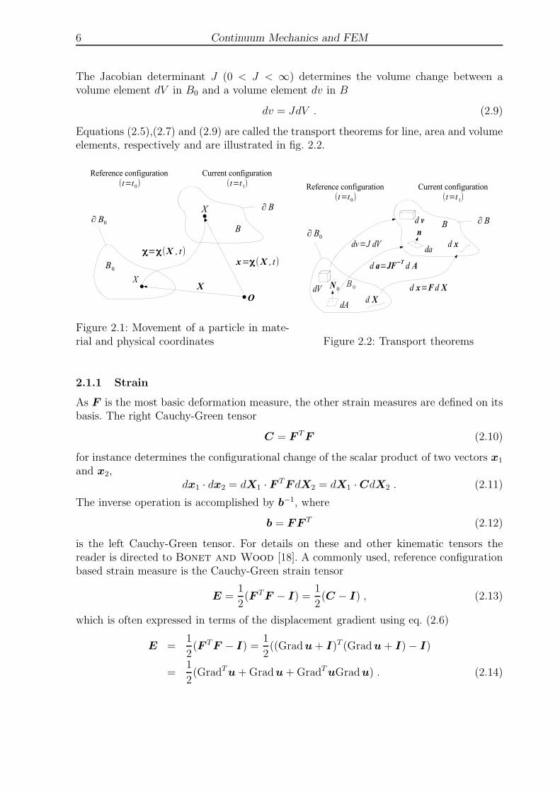
Equations (2.5),(2.7) and (2.9) are called the transport theorems for line, area and volumeelements, respectively and are illustrated in fig. 2.2.
Figure 2.1: Movement of a particle in mate-rial and physical coordinates Figure 2.2: Transport theorems
2.1.1 Strain
As F is the most basic deformation measure, the other strain measures are defined on itsbasis. The right Cauchy-Green tensor
C = F TF (2.10)
for instance determines the configurational change of the scalar product of two vectors x1
and x2,dx1 · dx2 = dX1 · F
TF dX2 = dX1 ·CdX2 . (2.11)
The inverse operation is accomplished by b−1, where
b = FF T (2.12)
is the left Cauchy-Green tensor. For details on these and other kinematic tensors thereader is directed to Bonet and Wood [18]. A commonly used, reference configurationbased strain measure is the Cauchy-Green strain tensor
E =1
2(F TF − I) =
1
2(C − I) , (2.13)
which is often expressed in terms of the displacement gradient using eq. (2.6)
E =1
2(F TF − I) =
1
2((Gradu+ I)T (Gradu+ I)− I)
=1
2(GradTu+Gradu+GradTuGradu) . (2.14)

Continuum Mechanics and FEM 7
Ignoring the quadratic contribution in eq. (2.14) gives the linear part of the strain
LinE =1
2(GradTu+Gradu) = sym(Gradu) , (2.15)
which is the symmetric part of the displacement gradient. This part purely refers todeformation whereas the additive skew-symmetric part refers to the rotational part of thetensor.
Applying the so-called covariant push-forward operation F−T (•)F−1 that transforms aquantity given in the reference configuration into the current configuration leads to theEuler-Almansi strain tensor
e = F−TEF−1 =1
2(I − b−1) . (2.16)
The inverse operation to a covariant push-forward is the covariant pull-back operationF T (•)F .
2.1.2 Stress
Cauchy’s fundamental lemma
t = σn (2.17)
states that the stress vector t is defined by a linear mapping of the outward normal vectorn, namely the Cauchy (or true) stress σ operating on n. Applying t to the area da leadsto
df = tda = σnda = σda , (2.18)
with df being a true force applied to the current area element da. The benefit of introduc-ing σ is that it does not contain information about the orientation, like the stress vector.Proper handling of the stress vector requires the knowledge of n, whereas the Cauchystress can be computed independent of the normal to the area element. From eq. (2.18)one derives the first Piola-Kirchhoff stress tensor by using the transport theorem (2.7)
df = σJF−TdA . (2.19)
Thus the first Piola-Kirchhoff stress tensor
P = σJF−T (2.20)
can be interpreted as the actual force applied to an area element in the reference configu-ration. Of course it is possible to transform the force itself to the reference configurationtoo which leads to
S = F −1P = JF−1σF−T , (2.21)
the second Piola-Kirchhoff stress tensor that represents a force mapped to the referenceconfiguration and applied to the reference configuration. S is often preferred because itis a symmetric tensor, unlike P .

8 Continuum Mechanics and FEM
Stress and strain can be related via a fourth-order constitutive tensor C
Σ = C(t, T, ε,α)ε (2.22)
that might be dependent on the time t, the temperature T , the strain ε or other parametersα. Throughout this thesis Voigt’s notation of symmetric stress and strain tensors will beused, i.e.
Σ = (Σ11,Σ22,Σ33,Σ12,Σ13,Σ23)T and (2.23)
ε = (ε11, ε22, ε33, 2ε12, 2ε13, 2ε23)T (2.24)
= (ε11, ε22, ε33, γ12, γ13, γ23)T , (2.25)
with γij being the shear strains and Σ and ε representing any conjugate stress and straintensors. A stress-strain pair (Σ, ε) is termed (work) conjugate if their double contractionequals the internally stored energy Ψ:
Σ : ε = Ψ . (2.26)
In the given notation the fourth-order constitutive tensor C is a square matrix.
2.2 Plate and Shell Theories
Plate and shell models are used to describe the kinematics of very thin bodies, whoselateral dimension l is much larger than its thickness h, i.e.
l >> h . (2.27)
A full three-dimensional discretization of such a plate either leads to very high length-thickness ratios or an unreasonably large number of elements, depending on whether itis a coarse or a fine mesh. In the former case one observes numerical locking whereasthe latter case leads to a highly increased number of degrees of freedom resulting inincreased computation time and increased memory consumption. In order to avoid thosecircumstances one degenerates the three-dimensional model into a middle plane with athickness h. A local, generally curvilinear coordinate system ξ = [ξ1, ξ2, ξ3] is attached tothis middle plane as shown in fig. 2.3, with in-plane coordinates ξ1 and ξ2, and ξ3 beingthe coordinate normal to the middle plane. If not otherwise stated, in this thesis, ξ isalways a Cartesian basis system because the developments herein are mainly based onplane plate models. In the case of shells one would switch to local curvilinear coordinatesin order to properly take into account the curvature of the shell geometry.
Due to the contents of the thesis the term plate is used rather than the term shell althoughall the concepts may be applied to shells too. The basic kinematic quantities of stan-dard plate and shell formulations are shown in fig. 2.3. The displacement u(ξ1, ξ2, ξ3) =[u1, u2, u3]
T of any point of the shell in general varies in thickness direction and dependson the translation v(ξ1, ξ2) = [v1, v2, v3]
T of the shell middle plane E(ξ1, ξ2, ξ3 = 0) andon its rotation in point (ξ1, ξ2, 0), termed w(ξ1, ξ2) = [w1, w2]
T = [θ2,−θ1]T .

Continuum Mechanics and FEM 9
2.2.1 Plate Models
In order to simplify the very general descripton of plates, different theories of varyingcomplexity have been introduced that are depicted in fig. 2.4 with respect to a beamexample (cross-section of a plate). The beam is clamped on its left end and on its rightend a moment M is applied.
Figure 2.3: Global and local coordinate sys-tems e and ξ, displacements vi, rotations wα
and normal n Figure 2.4: Plate theories
First of all the Kirchhoff-Love theory assumes that lines that initially are normal to theplate middle plane remain normal, i.e. the shell director d that is attached to the middleplane remains normal, shear strains are zero and it assumes constant thickness. Allowingfor transverse shear strains leads to so-called Reissner-Mindlin plates that usually assumea linearly varying displacement field in thickness direction ξ3
u = v + ξ3w , (2.28)
which can be written in detail for a local coordinate system ξ = [ξ1, ξ2, ξ3] tangential tothe plate middle plane,
u1(ξ1, ξ2, ξ3) = v1(ξ1, ξ2) + ξ3θ2(ξ1, ξ2) (2.29)
u2(ξ1, ξ2, ξ3) = v2(ξ1, ξ2) − ξ3θ1(ξ1, ξ2) (2.30)
u3(ξ1, ξ2, ξ3) = v3(ξ1, ξ2) . (2.31)
In both, the Kirchhoff-Love and the Reissner-Mindlin theory, the so-called Kirchhoffconstraint, ε33 = 0, leads to an inconsistency. Assuming plane stress, i.e. σ33 = 0, which is

10 Continuum Mechanics and FEM
a common assumption for the thin plate limit, one normally would be able to determineε33 from the constitutive eq. (2.22). The resulting non-zero thickness strain contradictsthe Kirchhoff constraint.
Consequently the next step in complexity of the formulation is the drop of the con-straint ε33 = 0 to get rid of this inconcistency. The so-called 7-parameter model in-troduces two new parameters into the variational form, namely the constant thick-ness strain χ and a strain component β33 that is linear in ξ3 to get a linearly vary-ing thickness strain. The variational form then is a three-field Hu-Washizu functionalas described in sect. 2.3.4.1. As β33 is introduced using the Enhanced Assumed Straintechnique and therefore does not need to be compatible, its parameters can be elimi-nated on element level. In fact the 7-parameter model ends up with a two-field func-tional as described in sect. 2.3.4.2. Plate and shell formulations including thickness strainhave already been the topic of many researchers and detailed explanations of the con-cept of 7-parameter models and the Enhanced Assumed Strain technique can be foundin Simo et al. [138], Simo and Armero [139], Buchter [21], Buchter et al. [22],Roehl [129], Betsch et al. [11], Bischoff [13], Miehe and Schroder [106] andKoschnick [85], to name only a selection. Those shell models share the benefit of beingable to use full three-dimensional constitutive laws for the shell without modification.
The last degree of complexity that is shown in fig. 2.4 is a nonlinear director d leading tomultilayer models. For details the reader is referred to Eckstein [46].
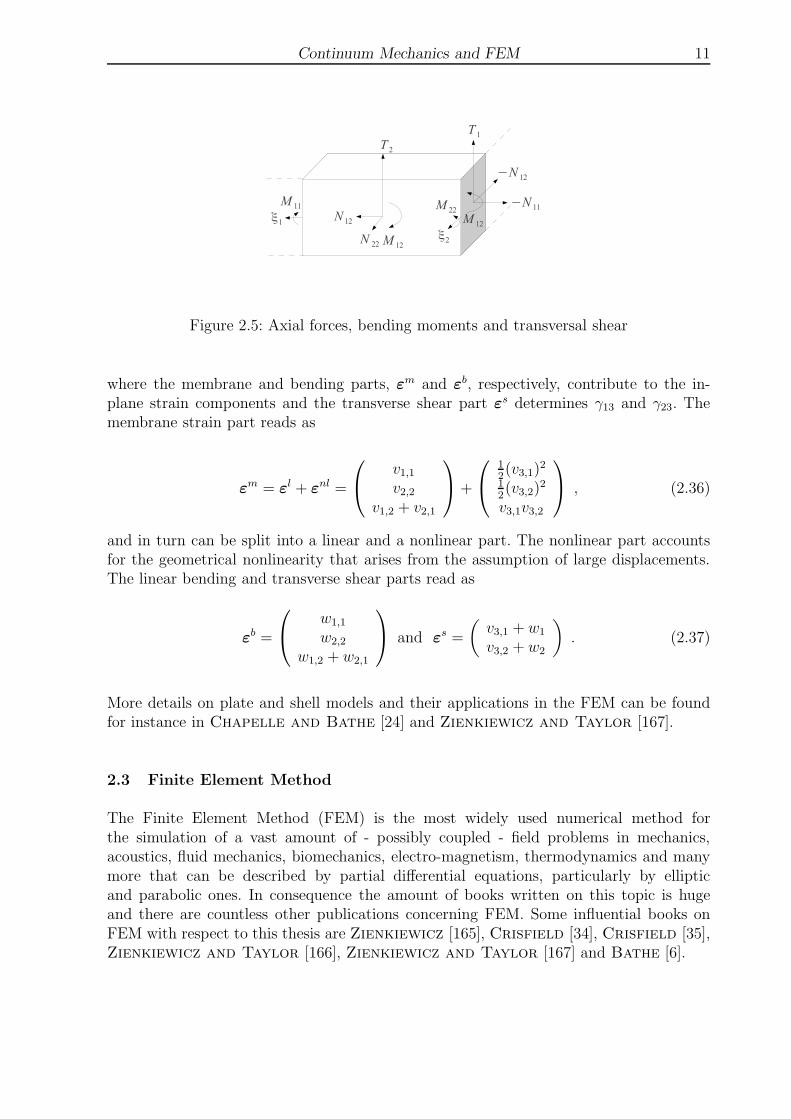
2.2.2 Reissner-Mindlin Plates in Detail
The Reissner-Mindlin plate theory is sufficiently accurate for the applications investigatedin this thesis. Figure 2.5 shows the stress resultants of a unit volume of a plate with respectto this theory. The stress resultants are
N =
N11
N22
N12
=
h2∫
−h2
σ11
σ22
σ12
dξ3 , (2.32)
M =
M11
M22
M12
=
h2∫
−h2
ξ3
σ11
σ22
σ12
dξ3 , (2.33)
T =
(T1
T2
)
=
h2∫
−h2
(σ13
σ23
)
dξ3 , (2.34)
with N ,M and T the axial forces, bending moments and transversal shear forces, re-spectively.
Therefore the strains are introduced as follows
ε = (ε11, ε22, γ12, γ13, γ23)T =
(εm
0
)
+
(ξ3ε
b
0
)
+
(0εs
)
, (2.35)
Continuum Mechanics and FEM 11
Figure 2.5: Axial forces, bending moments and transversal shear
where the membrane and bending parts, εm and εb, respectively, contribute to the in-plane strain components and the transverse shear part εs determines γ13 and γ23. Themembrane strain part reads as
εm = εl + εnl =
v1,1v2,2
v1,2 + v2,1
+
12(v3,1)
2
12(v3,2)
2
v3,1v3,2
, (2.36)
and in turn can be split into a linear and a nonlinear part. The nonlinear part accountsfor the geometrical nonlinearity that arises from the assumption of large displacements.The linear bending and transverse shear parts read as
εb =
w1,1
w2,2
w1,2 + w2,1
and εs =
(v3,1 + w1
v3,2 + w2
)
. (2.37)
More details on plate and shell models and their applications in the FEM can be foundfor instance in Chapelle and Bathe [24] and Zienkiewicz and Taylor [167].
2.3 Finite Element Method
The Finite Element Method (FEM) is the most widely used numerical method forthe simulation of a vast amount of - possibly coupled - field problems in mechanics,acoustics, fluid mechanics, biomechanics, electro-magnetism, thermodynamics and manymore that can be described by partial differential equations, particularly by ellipticand parabolic ones. In consequence the amount of books written on this topic is hugeand there are countless other publications concerning FEM. Some influential books onFEM with respect to this thesis are Zienkiewicz [165], Crisfield [34], Crisfield [35],Zienkiewicz and Taylor [166], Zienkiewicz and Taylor [167] and Bathe [6].
12 Continuum Mechanics and FEM
2.3.1 The Principle of Virtual Displacements
In elasticity the problem to be solved is given in its differential form as
divσ + f = 0 in Ω , (2.38)
u = u0 on Γu , (2.39)
σn = t0 on Γd , (2.40)
where eq. (2.38) is called the global balance of momentum and states the equilibriumof internal forces and external forces f . Both, f and the unknown displacement field u
need to be twice continuously differentiable. In addition, u has to fullfill the (essential)Dirichlet boundary conditions (2.39) and the (natural) Neumann boundary conditions(2.40). Robin (Newton) boundary conditions are a mixed kind and thus can be neglectedhere for simplicity. Equivalent formulations of this problem are the variational formulationand the herein employed principle of virtual displacements. Details on all formulationscan be found for instance in Bathe [6].
The principle of virtual displacements can be derived from the differential form by mul-tiplication with a test function δu and integration, i.e.
∫
Ω
divσ · δu dx+
∫
Ω
f · δu dx = 0 , (2.41)
which, using the symmetry of the stress tensor σ = σT , can be expanded to∫
Ω
div(σ · δu) dx−
∫
Ω
σ · gradδu dx+
∫
Ω
f · δu dx = 0 . (2.42)
The test function δu := ǫη is called the variation of u and is a non-zero function that hassimilar properties like u besides that it vanishes on Γ. In the limit case, by construction,
limǫ→0
(u+ δu) = limǫ→0
(u+ ǫη) = u , (2.43)
holds. Application of the divergence theorem to the first term in eq. (2.42) leads to∫
Γd
σn · δu ds−
∫
Ω
σ · δε dx+
∫
Ω
f · δu dx = 0 , (2.44)
where the symmetry of the stress tensor has been used again to get the equality gradδu =δε which is generally not true if σ were asymmetric. By rearranging one finally derivesthe principle of virtual displacements or the weak form of the differential formulation as
∫
Ω
σ · δε dx =
∫
Ω
f · δu dx+
∫
Γd
σn · δu ds , (2.45)
Finally inserting the constitutive relation (2.22) between stress and strain, the Neumannboundary condition (2.40) and switching to Voigt’s notation as introduced in sect. 2.1.2leads to ∫
Ω
δεTCε dx =
∫
Ω
δuTf dx+
∫
Γd
δuT t0 ds . (2.46)

Continuum Mechanics and FEM 13
The Dirichlet boundary conditions (2.39) are enforced globally and do not show up in theweak form (2.46). The main difference of the weak form to the differential form is thatthe unknown u needs to be only continuously differentiable now, i.e. u lies in the Sobolevspace
H1(Ω) = u|Dαu ∈ L2(Ω), ||α|| ≤ 1, (2.47)
with Dα the differential operator for all spatial dimensions indicated by α = α1, ..., αnand the Hilbert space
L2(Ω) = u|
∫
Ω
u2dΩ < ∞ (2.48)
of all square integrable functions. Summarizing this the function space of the solution is
S = u|u ∈ H1(Ω),u|Γu= u0,σn|Γd
= t0 . (2.49)
The function space of δu is similar but as already indicated, the function vanishes onΓ. Due to the lower requirements, the principle of virtual displacements and variationalapproaches are called weak forms whereas the differential form is called the strong form.
2.3.2 Variational Formulation
Although the formulations are fully equivalent, the variational formulation is shortly sum-marized here in order to provide the basics to show the variational consistency of S-FEMin sect. 3.2. Keeping in mind that the boundary conditions need to be fulfilled, the func-tional Π, being an energy potential, for a general problem can be written in the form
Π(u) =
∫
Ω
f
(
x,u,∂u
∂x
)
dx . (2.50)
It can be shown that the differential formulation is equivalent to the minimization of Π.The necessary condition for the functional to be minimal is that its first variation equalszero, i.e.
δΠ(u) =d
dǫΠ(u+ ǫη)
∣∣∣∣ǫ=0
= limǫ→0
1
ǫ(Π(u+ ǫη)− Π(u))
!= 0 , (2.51)
where the test function ǫη appears again.
2.3.3 Discretization
In order to solve the global eq. (2.45) FEM discretizes the computational domain Ω intoNE finite elements Ωe
i , with i = 1, ..., NE based on NN nodes. For the derivation of theelement equations a linear two-dimensional problem is addressed in order to keep it simple.The derivation of the equations for three-dimensional problems is straightforward and canbe found in Bathe [6]. The equations for plate problems will be shown in chap. 3.
Based on a discretization the local version of eq. (2.45) in Voigt’s notation reads as∫
Ωe
δεTσ dx =
∫
Ωe
δuTf dx+
∫
Γed
δuT t0 ds . (2.52)

14 Continuum Mechanics and FEM
By using the constitutive equation (2.22) as in eq. (2.46) and by switching to matrixnotation eq. (2.52) can be rewritten
∫
Ωe
δuTLTCLu dx =
∫
Ωe
δuT f dx+
∫
Γed
δuT t0 ds , (2.53)
with the differential operator
L =
∂∂x1
0
0 ∂∂x2
∂∂x2
∂∂x1
(2.54)
and the constitutive matrix C.
Up to here the field u is an element of the function space Sh ⊂ S, cf. eq. (2.49), whichonly contains the admissible functions regarding the discretization. Applying the Galerkinmethod, specific nodal shape functions ΦI are chosen to avoid searching for a solutionin the whole space Sh. Denoting Nn the number of nodes of an element, the discretedisplacement field and its variation can then be written on element level
ue(x) =Nn∑
I=1
ΦI(x)dI , (2.55)
δue(x) =Nn∑
I=1
ΦI(x)δdI , (2.56)
where the nodal shape functions ΦI have compact support on the respective elementonly and are applied to the respective nodal displacement vector dI . Summing up thecontributions of all NN nodes of the finite element mesh, one gets the global discretedisplacement field uh.
Herein the same shape functions for ue and δue are used (Bubnov-Galerkin method)although this is generally not required (Petrov-Galerkin method). For convenience theposition vector xe is represented in the same way as ue using the same shape functions.This approach is called the isoparametric concept. The application of the differentialoperator L to obtain the local strain field is straightforward
εe = Lue(x) =Nn∑
I=1
LΦI(x)dI =Nn∑
I=1
BI(x)dI , (2.57)
with the nodal strain-diplacement matrix BI containing the derivates of the shapefunctions. Using B = [B1, ...,BNn
], de = [d1, ...,dNn]T , δde = [δd1, ..., δdNn
]T , Φ =[Φ1, ...,ΦNn
] and the divergence theorem to integrate the boundary condition over theboundary only, eq. (2.53) can be reexpressed as
(δde)T∫
Ωe
BTCBde dx = (δde)T∫
Ωe
ΦT f dx+ (δde)T∫
Γd
ΦT t0 ds . (2.58)
Continuum Mechanics and FEM 15
The element stiffness matrix Ke and the right hand side of the equation system, Fe, thenread as
Ke =
∫
Ωe
BTCB dx , Fe =
∫
Ωe
ΦT f dx+
∫
Γd
ΦT t0 ds (2.59)
and the global version of eq. (2.58) is given as
(δd)T
NE
Ai=1
∫
Ωei
BTCB dx
d = (δd)T
NE
Ai=1
∫
Ωei
ΦT f dx+
∫
Γd
ΦT t0 ds
, (2.60)
where d = [d1, ...,dNN]T , δd = [δd1, ..., δdNN
]T and the operator A assembles the nodalcontributions of elements into the global stiffness matrix and into the global internal forcevector. In short terms, eq. (2.60) can be expressed as
Kd = F , (2.61)
withK,d and F being the global counterparts ofKe,de and Fe, respectively. The Dirichletboundary conditions are not part of the assembly as they prescribe the solution at certaindegrees of freedom and therefore need not to be computed.
The integration on element level usually is carried out using Gaussian integration basedon a certain number of weighted Gaussian points that are distributed within the element.The choice of the kind of Gaussian integration and the number of Gaussian points isdone with respect to the degree of the shape functions and the desired accuracy of thesolution. Moreover one usually performs the Gaussian integration on a parent element thatis defined in a natural coordinate system. Those details are not explained here becausethey are not relevant for this thesis. Details can be found in each of the references namedin the introduction of this chapter.
2.3.4 Special Principles of Potential Energy
According to Willner [157] the complete representation of the considered energy poten-tial is
Π(u) =1
2
∫
Ω
σ · ε dx−
∫
Ω
f · u dx−
∫
Γu
u0 · t ds−
∫
Γd
t0 · u ds , (2.62)
with traction vector t and u0 and t0 given by boundary conditions. It is called a 1-field functional because it solely depends on u. The necessary supplementary conditionsfor fully defining the linear problem are the expression of the strain in terms of thedisplacement gradient (2.15) and the constitutive equation (2.22).
There is a number of different energy potentials that directly integrate the supplementaryconditions into the potential thereby introducing more (Euler-Lagrange) differential equa-tions. Those potentials are the functional basis for methods like the already mentionedEnhanced Assumed Strain method or the Smoothed FEM (S-FEM) described in chap. 3.Both of the following energy potential formulations can be viewed as a functional basisof S-FEM, although chap. 3 only uses the 2-field de Veubeke functional.
16 Continuum Mechanics and FEM
2.3.4.1 Hu-Washizu The 3-field Hu-Washizu functional integrates both supple-mentary conditions (2.15) and (2.22) into the functional resulting in
Π(u, ε,σ) =1
2
∫
Ω
σ · ε dx −
∫
Ω
f · u dx−
∫
Γu
u0 · t ds−
∫
Γd
t0 · u ds
−
∫
Ω
(
ε−1
2(∇Tu+∇u)
)
· σ dx . (2.63)
In this functional all three fields are treated as unknowns. Using the supplementary con-dition (2.22) again to eliminate σ leads to the 2-field de Veubeke functional.
2.3.4.2 de Veubeke Using symmetry of the stress tensor and, for convenience,the constitutive tensor in tensor notation, it reads as
Π(u, ε) =1
2
∫
Ω
Cε · ε dx −
∫
Ω
f · u dx−
∫
Γu
u0 · t ds−
∫
Γd
t0 · u ds
−
∫
Ω
C
(
ε−1
2(∇Tu+∇u)
)
· ε dx
= −1
2
∫
Ω
Cε · ε dx +
∫
Ω
C
(1
2(∇Tu+∇u)
)
· ε dx
−
∫
Ω
f · u dx−
∫
Γu
u0 · t ds−
∫
Γd
t0 · u ds . (2.64)
Willner [157] explains that this functional formerly has been called the Reissner prin-ciple but that it should be named after de Veubeke. Liu and Nguyen [95] even call itHellinger-Reissner principle. Within this thesis a functional Π(u,σ) is called a Hellinger-Reissner functional.
The variation of the de Veubeke potential energy
δΠ(u, ε) = −1
2
∫
Ω
Cεδε dx +
∫
Ω
C
(1
2(∇Tu+∇u)
)
· δε dx
−
∫
Ω
f · δu dx−
∫
Γu
u0 · δt ds−
∫
Γd
t0 · δu ds (2.65)
delivers the principle of virtual displacements that is later used for the variationally con-sistent derivation of S-FEM. The nonlinear variational form is straightforward and canbe found in Willner [157].
2.3.5 Nonlinear FEM
The derivation of the principle of virtual displacements for geometrically nonlinear three-dimensional problems can be found in e.g. Crisfield [34] and Bathe [6], the latter of

Continuum Mechanics and FEM 17
which is the foundation of this section. Geometrically nonlinear plate problems can beviewed as a special case of a three-dimensional problem, thus here the principle for thethree-dimensional case is derived.
For the nonlinear case we rewrite the linear principle of virtual displacements (2.45), stayin Voigt’s notation for convenience and seek for an incremental solution ut+∆t at timet+∆t that satisfies ∫
Ω
δεTt+∆tσt+∆t dx = Rt+∆t , (2.66)
with Rt+∆t containing the body forces and the static boundary conditions. Assumingthat ε is nonlinear now, one has to linearize eq. (2.66) using Taylor series expansion at adegree of freedom uj. With an incremental change, ∆uj, the linearization of the integrandis given as
δεTt+∆tσt+∆t = δεTt σt +∂(δεTt σt
)
∂uj
∆uj . (2.67)
From this notation it becomes apparent that in the incremental procedure, computablequantities at time t are employed to compute the solution at time t+∆t. Moreover, dueto the nonlinearity of the problem, the accuracy of the solution strongly depends on thetime step ∆t. Keeping this in mind, in the sequel the time information is dropped forcompactness. Using the following property of a variation
δε =∂ε
∂uj
δuj , (2.68)
the second term in eq. (2.67) can be differentiated and simplified as follows
∂(δεTσ
)
∂uj
∆uj =
(∂δεT
∂uj
σ + δεT∂σ
∂uj
)
∆uj
=
(
δuTj
∂2εT
∂u2j
σ + δuTj
∂εT
∂uj
∂σ
∂ε
∂ε
∂uj
)
∆uj
= δuTj
(∂2εT
∂u2j
σ +∂εT
∂uj
C∂ε
∂uj
)
∆uj , (2.69)
which leads to the linearized principle of virtual displacements
δuTj
∫
Ω
∂εT
∂uj
σ dx+ δuTj
∫
Ω
(∂2εT
∂u2j
σ +∂εT
∂uj
C∂ε
∂uj
)
dx∆uj = R (2.70)
or
δuTj
∫
Ω
(∂2εT
∂u2j
σ +∂εT
∂uj
C∂ε
∂uj
)
dx∆uj = R− δuTj
∫
Ω
∂εT
∂uj
σ dx . (2.71)
The second term on the left hand side is called the material stiffness as before. Thefirst term arises from the geometrical nonlinearity and therefore is called the geometricalstiffness. On the right hand side an additional term appears in the nonlinear formulationthat can be identified with internal forces.

18 Continuum Mechanics and FEM
The nonlinear global principle of virtual work can now be expressed using the matricesknown from the linear FEM. It reads as
(Km +Kg)d = R− F , (2.72)
with the global material and geometrical stiffness matrices Km and Kg, respectively, orin more detail
∫
Ω
BTCB dx+
∫
Ω
GTSG dx
d = R−
∫
Ω
BTS dx , (2.73)
where B now is the nonlinear strain-displacement matrix related to the nonlinear strain(2.14) and G contains derivatives of shape functions. Finally, S is a matrix of stresscomponents, such that the second term on the right hand side of eq. (2.73) represents theinternal forces. Detailed expressions of the respective matrices are omitted here becausefor geometrically nonlinear plate problems they are given in sect. 3.4.
2.3.6 Finite Element Discretization of Plates and Shells
As it is apparent from the cited references, FE discretizations exist for any of the theoriesshown in fig. 2.4. In this thesis the Reissner-Mindlin theory has been applied and twodifferent FE discretizations have been used. Both of them use triangular elements becausea robust automatic meshing is required for biomechanical applications in general, althoughnot necessarily for the particular model built here. In terms of standard FEM the shapefunctions are of degree two whereas in the context of S-FEM only linear shape functionsare employed. In the latter case the disadvantages of constant strain triangular elementsare greatly reduced by S-FEM.
Both discretizations introduce six degrees of freedom per node, three of which are trans-lational and two of which are rotational. The sixth degree of freedom does not have aphysical meaning and the related stiffness is chosen very small to only marginally influ-ence the result but sufficiently large to avoid ill conditioning.

Smoothed FEM 19
3 Smoothed FEM
The FE modeling of biological tissue possesses some general difficulties:
Mesh quality: First of all the mesh quality often is bad, i.e. one expects high aspectratios of the inner angles of at least some elements. With respect to soft biologicaltissues there are some possible reasons for a bad mesh quality:
1. The considered geometries defined by the problem domain usually can not bediscretized with other elements than triangles or tetrahedrals because of theircomplexity. Patient-specific geometrical data from X-Ray, MRI, CT, plasti-nates or similar imaging procedures usually result in geometrical data wheremost of the automatic meshing algorithms fail. Even requiring some manualrepairing, the only class of meshing algorithm that is able to reliably producea valid FE mesh, is triangulation in 2D and 3D. Besides the fact that a com-mon triangulation in those cases usually produces some elements with highaspect ratios between the inner angles of the triangle, in general triangular, aswell as tetrahedral meshes are known to have a worse performance than theirquadrilateral and hexahedral counterparts, respectively.
2. Even if the automatic and manual efforts result in a reasonable mesh quality,difficulties arise during deformation. Soft biological tissues undergo large defor-mations that again lead to high aspect ratios. Even more so if some elementsalready have high aspect ratios that become even higher. Unfortunately onebadly shaped element already leads to computational problems or even abor-tion of the computation. Remeshing is a possible but very expensive remedyin terms of computation time.
3. The simulation of cutting soft tissues is done in real-time for surgical trainingpurposes. Cutting eventually produces badly shaped elements that have to behandled with caution.
In the best case, if the computation does not abort due to a singularity, shearlocking might occur because of the distorted elements, resulting in highly inaccuratedeformation behaviour.
Incompressibility: Biological soft tissues often are (quasi-)incompressible, i.e. J =det(F ) ≈ 1, which leads to the volumetric locking phenomenon in a standard FEsetup. To overcome this problem some techniques already exist, like underintegratedelements. A comprehensive and well-written overview of these techniques is given inKoschnick [85]. In order to impose incompressibility the constitutive tensor canbe decomposed into a deviatoric and a volumetric part (cf. Holzapfel [72]).
Transverse shear locking: With respect to the thin plate problem that is investi-gated in this thesis another locking phenomenon occurs, namely the transverse shearlocking. It occurs in the computation of very thin structures and leads to inaccuratedeformation behaviour too. This locking phenomenon stiffens the system and the

20 Smoothed FEM
computed deformation is often much smaller than the real deformation. There areadvanced techniques to remedy this locking phenomenon like the Discrete ShearGap method presented in Bletzinger et al. [14].
Most of the named problems lead to some kind of locking. A very informative andcomprehensive thesis on locking phenomena and their treatment has been written byKoschnick [85]. One way to overcome all the named problems at the same time is theso-called smoothed FEM (S-FEM). S-FEM is a class of methods that bases on the ideaof strain smoothing. Chen et al. [25] started to apply this idea to avoid material in-stabilities in meshless methods and Chen et al. [26] proposed to use strain smoothingfor stabilizing nodal integration. Since then, S-FEM has been developed and a collectionof S-FEM theory and computational examples can be found in Liu and Nguyen [95].There is a large number of different kinds of S-FEM with different benefits and draw-backs that are explained in detail in Liu and Nguyen [95] too. Some of them arepresented in sect. 3.3. Moreover there is a number of publications covering differ-ent topics concerning S-FEM, like Cui et al. [36], Dai and Liu [39], Dai et al. [40],Liu et al. [96] and Liu et al. [97] that construct S-FEM for various 2D prob-lems, Cui et al. [38], Frotscher and Staat [50] and Nguyen-Xuan et al. [113]that apply S-FEM on plates and shells, Bordas et al. [19], Chen et al. [27],Liu et al. [94] and Nix et al. [118] where S-FEM is combined with the extended FEMand for instance Nguyen-Thoi et al. [112] where the face-based S-FEM is introducedfor 3D problems.
Within this thesis the so-called edge-based Smoothed Finite Element Method (ES-FEM)is applied to the nonlinear plate problems because this method shows a very good accuracywhen applied to linear triangular elements, it is insensitive to element distortion and itovercomes shear locking naturally. Before the ES-FEM becomes explained in detail, theidea of strain smoothing and the variational details for S-FEM are presented. Some partsof this chapter already appeared in Frotscher et al. [54] and are repeated here withsome modifications.
3.1 Strain Smoothing
All different kinds of S-FEM share the idea of smoothing the strain over so-called smooth-ing domains Ωs
i
εi = ε(xi) =
∫
Ωsi
W (xi − x)ε(x) dΩ , (3.1)
with ε being the usual, possibly known, (compatible) strain, W representing a scalarweighting function and εi being the smoothed strain in Ωs
i . In order to stay consistentwith the FEM the smoothing domains are non-overlapping, i.e. Ωs
i ∩ Ωsj = ∅(i 6= j) but
fully cover the computational domain, i.e. Ωs1 ∪ · · · ∪ Ωs
Ns= Ω, where Ns is the total
number of smoothing domains. Usually W is chosen in the way that the smoothed strain

Smoothed FEM 21
in eq. (3.1) becomes an area-weighted average of the strains in the smoothing domain
W (xi − x) =
1As
i
, x ∈ Ωsi
0, x 6∈ Ωsi
, (3.2)
with Asi the area of the i-th smoothing domain. In the case of a plate problem we can
apply eq. (3.1) to each strain part separately using eq. (3.2) to get
εli =1
Asi
∫
Ωsi
εli(x) dΩ , (3.3)
εbi =1
Asi
∫
Ωsi
εbi(x) dΩ , (3.4)
εsi =1
Asi
∫
Ωsi
εsi (x) dΩ , (3.5)
εnli =1
Asi
∫
Ωsi
εnli (x) dΩ , (3.6)
with εli, εbi , ε
si , ε
nli the smoothed linear membrane, bending, shear and nonlinear strain
parts, respectively.
In eqs. (3.1) and (3.3)–(3.6) a known strain ε becomes smoothed. One way of getting aknown strain field is to perform a standard FE computation and smooth the compatiblestrain afterwards. In this case the S-FEM is boiled down to a simple averaging procedure.As the reader will see below it is more advantageous to avoid the smoothing of thecompatible strain and compute the smoothed strain directly instead. The principle ideaof strain smoothing can easily be explained with respect to the smoothed linear membranestrain and the same procedure can be applied to the other smoothed strain parts too. Toget to the discretized equations, first the compatible strain is replaced by an unknownstrain that can be computed using the differential operator Ld
εl(xi) =
∫
Ωsi
Ldu(x)W (xi − x) dΩ . (3.7)
Using integration by parts one can transform the domain integral in eq. (3.7) into anintegral over the boundary Γs
i of the smoothing domain
εl(xi) =
∫
Γsi
Ln(x)u(x)W (xi − x) dΓ−
∫
Ωsi
u(x) W (xi − x)︸ ︷︷ ︸
=0
dΩ
=1
Asi
∫
Γsi
n1 00 n2
n2 n1
︸ ︷︷ ︸
Ln(x)
u(x) dΓ ∀x ∈ Ωsi . (3.8)
22 Smoothed FEM
It is apparent that Ln contains the components of the outward normal vector on theboundary of the smoothing domain and that the strains are no longer the symmetric partof the displacement gradient because no derivatives of shape functions are involved in eq.(3.8). The next step would be to derive the discretized equations but first the variationalbasis of S-FEM is derived and further the smoothing domain creation is adressed.
3.2 Smoothed Galerkin Weak Form
Liu and Nguyen [95] derive the smoothed Galerkin weak form from the 2-field deVeubeke variational principle although therein it is called the Hellinger-Reissner prin-ciple. Assuming an admissible strain field ε that can be obtained from the displacementfield u the de Veubeke variational principle (cf. eq. (2.65)) degenerates into a 1-fieldvariational principle. Its variation in Voigt’s notation on smoothing domain Ωs
i reads as
δΠ(u)|Ωsi
= δ
−
1
2
∫
Ωsi
εiT (u)Cεi(u) dx+
∫
Ωsi
εiT (u)C (Lu) dx
−
∫
Ω
δuTf dx−
∫
Γu
δtTu0 ds−
∫
Γd
δuT t0 ds , (3.9)
with a differential operator L. Taking into account the assumption that the smoothedstrain ε is constant within a smoothing domain leads to
∫
Ωsi
εiT (u)C (Lu) dx = εi
T (u)CAsiLu =
∫
Ωsi
εiT (u)Cεi(u) dx . (3.10)
Reinserting this into eq. (3.9) and using a similar assembly process as in standard FEMto get the global discretized weak form one gets
δΠ(u) = δ
Ns
Ai=1
1
2
∫
Ωsi
εiT (u)Cεi(u) dx
−
∫
Ω
δuTf dx−
∫
Γu
δtTu0 ds−
∫
Γd
δuT t0 ds . (3.11)
For the linear part of the smoothed strain one inserts eq. (3.8) into eq. (3.11), which leadsto
δΠ(u) =
Ns
Ai=1
1
Asi
∫
Γsi
(Lnδu)TC(Lnu) dx
−
∫
Ω
δuTf dx−
∫
Γu
δtTu0 ds−
∫
Γd
δuT t0 ds . (3.12)
Smoothed FEM 23
This variational form can now be specialized for any kind of S-FEM by choosing therespective smoothing domains. The most important message from this section is thatS-FEM methods are variationally consistent because they can be derived from the deVeubeke variational form.
3.3 Smoothing Domains
So far the shape or creation of the smoothing domains have not been adressed. The basicS-FEM kinds are the cell-based (CS-FEM), the node-based (NS-FEM) and the edge-based(ES-FEM) S-FEM for 2D meshes and the face-based (FS-FEM) S-FEM for 3D meshes.Those methods solely differ in the creation of the smoothing domains thereby creatingdifferent advantages. Combinations of different kinds of S-FEM to get the benefits in thepart of the mesh where they are needed or direct combination of the methods on smoothingdomain level (αS-FEM) already have been developed by Liu and Nguyen [95].
All the methods have in common that they create their smoothing domains based on astandard FE mesh constisting of linear elements, without the introduction of additionalnodes or degrees of freedom. Within the smoothing domains a constant strain is assumed.Figure 3.1 depicts four possible ways of smoothing domain creation in the case of CS-FEM. CS-FEM can be applied to quadrilateral elements by subdividing each element Ωe
i
into a number of smoothing cells Ωsie, with ie depending on the respective element. Cell-
based smoothing domains are formed by taking the nodes of the finite element and virtualnodes on the element boundary as well as inside the element as corner points of the cells.The way of subdivision and the number of smoothing cells should be chosen with respectto stability requirements. Regarding stability there is an optimal number of smoothingcells per element. Figure 3.1 shows a quadrilateral element that has been subdivided into1,2,3 and 4 smoothing cells.
Figure 3.2 shows that node-based smoothing domains are created around each node of theFE mesh by taking the barycenters of the elements surrounding the respective node andthe midpoints of each edge connected to the node as the cornerpoints of the smoothingdomain. The special property of NS-FEM is that it is free of volumetric locking. Thereforethe selective combination of CS-FEM and NS-FEM to NCS-FEM is very beneficial to havethe stability and accuracy of CS-FEM and to get rid of the volumetric locking where itoccurs.
Figure 3.3 shows a middle plane of a plate that is meshed with three triangular elementsbased on four nodes A, B, C and D. Two edge-based smoothing domains Ωs
k and Ωsm
are highlighted here; the former one bases on edge k and the latter one on edge m ofthe standard finite element mesh. Both are formed using the two corner nodes of therespective edge and the barycenters of the element(s) connected to the respective edge.Please note that, as in any of the S-FEM kinds, the barycenters are virtual nodes thusthey do not carry additional degrees of freedom. Concerning the discretization there is nodifference between 2D and plate problems despite from the number of degrees of freedoms.The ES-FEM and its benefits are explained in detail in sect. 3.4 because it is the methodof choice with respect to the computation of soft biological tissues. The last basic S-FEM

24 Smoothed FEM
a) b)
c) d)
Figure 3.1: Cell-based smoothing domains
Node k
Figure 3.2: Node-based smoothing domains
Figure 3.3: Edge-based smoothing domains Figure 3.4: Face-based smoothing domains
kind is the FS-FEM, shown in fig. 3.4. It is the 3D equivalent of ES-FEM and basicallyhas the same properties.
3.4 Edge-based S-FEM for Nonlinear Plate Problems
Equation (3.12) reveals that the integration is now performed on smoothing domains in-stead of elements. Besides the fact that the local quantities now lie on smoothing domainsthe discretization of eq. (3.8) looks quite familiar:
εl(xi) =Nn∑
I=1
Bl
I(xi)dI , (3.13)
with Nn being the number of nodes related to the smoothing domain, Bl
I being therespective smoothed strain-displacement matrix and dI being the nodal vector of degreesof freedom at node I. For plate problems each nodal dI = [dI1, dI2, dI3, dI4, dI5]
T containstwo in-plane translational, one out-of-plane translational and two rotational degrees offreedom according to the plate kinematics given by eqs. (2.29)–(2.31). Regarding theexample in fig. 3.3 Nn takes the values 3 for Ωs
m and 4 for Ωsk. An inner smoothing

Smoothed FEM 25
domain like Ωsk occupies space in two different elements thereby relating all the nodes of
both elements. As a consequence the local stiffness matrix on Ωsk has an increased size
compared to standard FEM leading to an increased bandwidth of the global matrices.
Please note that for the computation of the global smoothed displacement field u, the Nstandard nodal shape functions are employed and that the isoparametric concept is stillused. N is the total number of nodes in the FE mesh. From eqs. (3.8) and (3.13) it is nowpossible to construct
Bl
I(xi) =1
Asi
∫
Γsi
Ln(x)ΦI(x) dΓ =
bI1 0 0 0 00 bI2 0 0 0bI2 bI1 0 0 0
, (3.14)
with
Ln(x) =
n1(x) 0 0 0 00 n2(x) 0 0 0
n2(x) n1(x) 0 0 0
(3.15)
containing the components of the outwards directed normal vector on the boundary ofthe smoothing domain. The structure of Ln differs with respect to the respective part ofthe strain (cf. eqs. (3.19)–(3.21)). The entries of the smoothed strain-displacement matrixread as
bI(xi) =1
Asi
∫
Γsi
ΦI(x)ni(x) dΓ . (3.16)
Placing Gauss Points in the center of each boundary segment of the smoothing domain(e.g. Γs
k and Γsm in fig. 3.3) one discretizes the remaining boundary integral to get
bI(xi) =1
Asi
Ns∑
k=1
ΦI(xGPk )ni(x
GPk )lk , (3.17)
with Ns being the number of boundary segments, xGPk the Gaussian Point at the center
of segment Γk, ni the outward normal vector and lk the length of segment Γk. Of course,like in standard FEM the number of Gaussian Points and also their placement can vary.Regarding the fact that the strain is assumed to be constant within a smoothing domainthe placement of one Gaussian Point at the center of each boundary segment is sufficient.Concerning applications that have to deal with discontinuities (Smoothed X-FEM) moreGaussian Points are used and differently distributed within the smoothing domain in orderto better resolve close to the discontinuity.
It has been mentioned earlier that computing the smoothed strain from eq. (3.13) ratherthan using a known compatible strain field is beneficial. The first reason is that thecomputation of BI does not require derivatives of shape functions. The shape functionsthemselves are sufficient due to the boundary integral formulation. Secondly, with thechoice of linear triangular elements all quantities are computed in physical coordinatesthus isoparametric mappings are avoided.

26 Smoothed FEM
The given procedure applies to the other parts of B too thus the smoothed strain-displacement matrix for smoothing domain Ωs
i reads as
Bi =
Bl
i + Bnl
i
Bb
i
Bs
i
, (3.18)
with Bi = [B1, ..., BNn]. B
l
I has already been given in eq. (3.14). The other parts of thesmoothed strain are
Bb
I =
0 0 0 0 bI10 0 0 −bI2 00 0 0 −bI1 bI2
, (3.19)
Bs
I =
0 0 bI11Nn
Nn∑
j=1
ΦI(xj) 0
0 0 bI2 0 1Nn
Nn∑
j=1
ΦI(xj)
, (3.20)
Bnl
I =
Nn∑
J=1
bJ1ωJ 00 bJ2ωJ
bJ2ωJ bJ1ωJ
[0 0 bI1 0 00 0 bI2 0 0
]
, (3.21)
with ωJ the nodal deflection. The sum in eq. (3.21) represents the smoothed displacementgradient. The smoothing of which is similar to that of the strain. Starting from
H(xi) =
∫
Ωsi
∂u
∂xW (xi − x) dx
=
∫
Γsi
LnuW (xi − x) dx−
∫
Ωsi
uW (xi − x) dx
=1
Asi
∫
Γsi
Lnu dx , (3.22)
the discretized smoothed displacement gradient applied to the deflection component onlyreads as
H(xi) =
Nn∑
I=1
BIwI . (3.23)
Figure 3.5 shows the different coordinate systems that are needed for the computationbesides the global coordinate system, i.e. the element coordinate systems ξ1 and ξ2 aswell as a smoothing domain coordinate system ξ1.
With respect to fig. 3.5 one can sum up the computation of Bi as follows. Both smoothedstrain-displacement matrices B1 and B2 are computed on element level in the respectiveelement coordinate system and transformed into the smoothing domain coordinate system
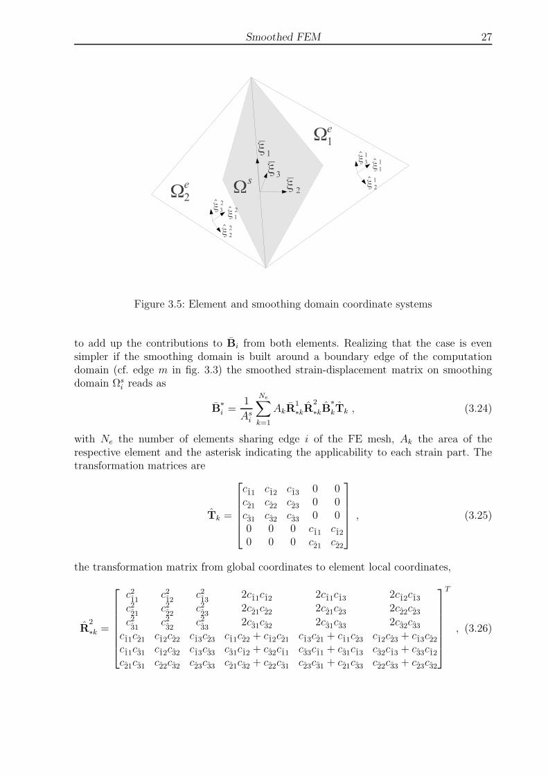
Smoothed FEM 27
Figure 3.5: Element and smoothing domain coordinate systems
to add up the contributions to Bi from both elements. Realizing that the case is evensimpler if the smoothing domain is built around a boundary edge of the computationdomain (cf. edge m in fig. 3.3) the smoothed strain-displacement matrix on smoothingdomain Ωs
i reads as
B∗
i =1
Asi
Ne∑
k=1
AkR1∗kR
2
∗kB∗
kTk , (3.24)
with Ne the number of elements sharing edge i of the FE mesh, Ak the area of therespective element and the asterisk indicating the applicability to each strain part. Thetransformation matrices are
Tk =
c11 c12 c13 0 0c21 c22 c23 0 0c31 c32 c33 0 00 0 0 c11 c120 0 0 c21 c22
, (3.25)
the transformation matrix from global coordinates to element local coordinates,
R2
∗k =
c211
c212
c213
2c11c12 2c11c13 2c12c13c221
c222
c223
2c21c22 2c21c23 2c22c23c231
c232
c233
2c31c32 2c31c33 2c32c33c11c21 c12c22 c13c23 c11c22 + c12c21 c13c21 + c11c23 c12c23 + c13c22c11c31 c12c32 c13c33 c31c12 + c32c11 c33c11 + c31c13 c32c13 + c33c12c21c31 c22c32 c23c33 c21c32 + c22c31 c23c31 + c21c33 c22c33 + c23c32
T
, (3.26)

28 Smoothed FEM
the rotation matrix from element to global coordinates and
R1∗k =
c211 c212 c213 c11c12 c11c13 c12c13c221 c222 c223 c21c22 c21c23 c22c23c231 c232 c233 c31c32 c31c33 c32c33
2c11c21 2c12c22 2c13c23 c11c22 + c12c21 c13c21 + c11c23 c12c23 + c13c222c11c31 2c12c32 2c13c33 c31c12 + c32c11 c33c11 + c31c13 c32c13 + c33c122c21c31 2c22c32 2c23c33 c21c32 + c22c31 c23c31 + c21c33 c22c33 + c23c32
,
(3.27)the rotation matrix from global to smoothing domain coordinates.
The global smoothed tangent stiffness matrix in the smoothing domain coordinate systemthen is given by
Kt
IJ =
Ns∑
i=1
(Bi
)T
IC(Bi
)
JAs
i +
Ns∑
i=1
(Gi
)T
IN(Gi
)
JAs
i , (3.28)
with Ns the number of smoothing domains, i.e. edges in the mesh. The second term ineq. (3.28) is the smoothed geometrical stiffness matrix and consists of
(Gi
)
I=
[0 0 bI1 0 00 0 bI2 0 0
]
(3.29)
and the matrix of the membrane stress resultants
N =
[N11 N12
N12 N22
]
. (3.30)
According to eq. (2.73) the nodal force vector given in the coordinate system ξ can becomputed from
FI =Ns∑
i=1
(Bi
)T
I
N
M
T
I
, (3.31)
where N,M and T are the discrete axial forces, bending moments and transverse shearforces (cf. eqs. (2.32)–(2.34)). Given that the boundary conditions are integrated as usual(e.g. by elimination or by Lagrangian coefficients) the global system of equations that hasto be solved reads as
Ktd = F . (3.32)
The assembly process for the stiffness matrix and the internal force vector is similar to thatof standard FEM although some remarks are indicated. In this work the smoothed localtangent stiffness matrices K
t
i are directly assembled into the global smoothed tangent
stiffness matrix. It should be noticed that Kt∈ R5N×5N (five degrees of freedom per
node) has exactly the same size as the standard tangent stiffness matrix whereas the size
of the smoothed local tangent stiffness matrices Kt
i ∈ R5Nn×5Nn depends on whether therespective smoothing domain is related to an inner edge or an edge on the boundaryof the FE mesh. For a mesh consisting of linear triangular elements, in the latter case
Smoothed FEM 29
Kt
i contributes to three nodes only, i.e. Nn = 3, whereas in the former one Nn = 4,
leading to an increased bandwidth of Kt. The proposed smoothing domain-based assembly
necessitates a modification of the standard implementation of the assembly process. Thiscan be avoided by splitting up K
t
i into element-wise contributions as for instance done inCui et al. [37].
For completeness, the final remark concerns the sixth, unphysical degree of freedom at eachnode, that was already mentioned in sect. 2.3.6. For numerical reasons it is also includedin the presented ES-FEM formulation but it has not been shown for compactness.
3.5 Involving the Discrete Shear Gap Method
It has already been shown in sect. 2.2.2 that each component of the shear strain,
εs =
(v3,1 + w1
v3,2 + w2
)
, (3.33)
is computed from the sum of the first derivative of a displacement v and from a rotationw. For plates one often states the so-called Kirchhoff constraint that requires
γ = v′ + w = 0 . (3.34)
However, this is usually in contradiction to the reality which becomes apparent if purebending is regarded. In the case of pure bending the transverse shear stresses vanish, i.e intheory eq. (3.34) is satisfied but regarding a discretization this is usually not true. Usuallythe displacements and the rotations are discretized using the same shape functions or atleast shape functions of equal degree. One can directly see that this violates the Kirchhoffconstraint because after discretization v′ is one degree lower than w, i.e.
γ = v′ + w 6= 0 . (3.35)
This discrepancy that causes transverse shear locking has been adressed by many differentapproaches that are detailed and compared in Koschnick [85]. One of the most simpleapproaches has been published in Bletzinger et al. [14] and is called the DiscreteShear Gap (DSG) method. This method introduces a discretized shear gap field on elementlevel that later can be condensed in order to keep the number of degrees of freedom ofthe element. In a linear triangular element, the discretized shear gap field removes thelinear part of the transverse shear which results from the discretization and makes itconstant. This way no parasitic shear stresses occur anymore and transverse shear lockingis effectively avoided. The DSG method has been generalized for other strain parts inKoschnick et al. [86] and is called the Discrete Strain Gap method then.
The ES-FEM triangular plate element employed in this thesis is enhanced by the DSGmethod. The only thing that changes on element level, is the computation of the shearpart of the strain-displacement matrix thus this method can be called a B-bar method.The respective shear strain, εsDSG replaces the standard shear strain on element level. Itreads as
εsDSG = BsDSG[d1,d2,d3]
T , (3.36)
30 Smoothed FEM
with BsDSG that has already been presented in Nguyen-Xuan et al. [114] and
Cui et al. [37] and is shown here for the sake of completeness. BsDSG is composed of
three nodal parts, thus BsDSG = [Bs1
DSG,Bs2DSG,B
s3DSG], with
Bs1DSG =
1
2Ak
[0 0 b− d 0 Ak
0 0 c− a −Ak 0
]
(3.37)
Bs2DSG =
1
2Ak
[0 0 d − bd
2ad2
0 0 −c bc2
−ac2
]
(3.38)
Bs3DSG =
1
2Ak
[0 0 −b bd
2− bc
2
0 0 a −ad2
ac2
]
. (3.39)
The parameters a = x2 − x1, b = y2 − y1, c = x3 − x1 and d = y3 − y1 are computed fromthe nodal coordinates of the element and Ak is the area of the element. As this method isa B-bar method, nothing changes in the smoothing of this strain part, i.e. eq. (3.24) canbe applied to get the respective smoothed strain-displacement matrix.

Cardiac Cells and Tissue 31
4 Cardiac Cells and Tissue
This section is intended to provide an overview over human cardiac tissue and cardiaccells as far as it is needed to understand their electrophysiology.
The human heart is an autonomously beating organ as depicted in fig. 4.1 and as mostbiological tissues each tissue in the human heart consists of a collagen-based extracellularmatrix (ECM) and embedded cells. Both, the ECM and the respective cardiac cells areunder investigation because they fulfill different tasks. The ECMmainly provides a passivestiffness of the tissue whereas the contribution of cells to the passive stiffness of thetissue is negligible. Cardiac cells mainly provide an active contribution to the stiffness bycontraction, be it self-induced or triggered. This thesis investigates the contractile behaviorof cardiac cells and therefore the ECM is not explained in further detail. However, itshould be noticed that the composition of the ECM in fact strongly influences the overallcontractile strength of the tissue.
Figure 4.1: The anatomy of the human heart (Credits: Ties van Brussel, public domain)
Cardiac cells consist of overlapping actin and myosin filaments. They are attached viaso-called cross bridges. The overlap is strain dependent thus if the tissue is stretched theactin and myosin myofilaments overlap less and the stress produced is higher.
The constituent of the heart that is responsible for generating the electrical stimulus iscalled sinoatrial node (SA node), cf. fig. 4.2. The dominating cells in the SA node areauto-contractile sinoatrial cells. The electrophysiology of SA cells is balanced in a way so
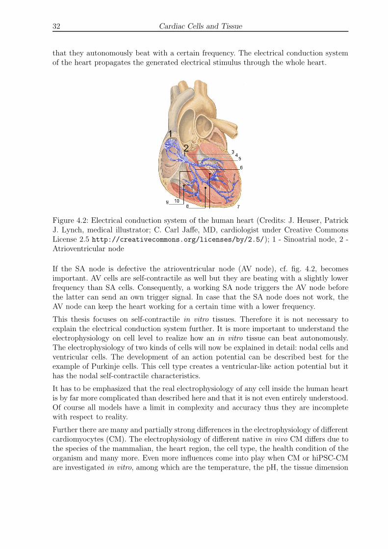
32 Cardiac Cells and Tissue
that they autonomously beat with a certain frequency. The electrical conduction systemof the heart propagates the generated electrical stimulus through the whole heart.
Figure 4.2: Electrical conduction system of the human heart (Credits: J. Heuser, PatrickJ. Lynch, medical illustrator; C. Carl Jaffe, MD, cardiologist under Creative CommonsLicense 2.5 http://creativecommons.org/licenses/by/2.5/); 1 - Sinoatrial node, 2 -Atrioventricular node
If the SA node is defective the atrioventricular node (AV node), cf. fig. 4.2, becomesimportant. AV cells are self-contractile as well but they are beating with a slightly lowerfrequency than SA cells. Consequently, a working SA node triggers the AV node beforethe latter can send an own trigger signal. In case that the SA node does not work, theAV node can keep the heart working for a certain time with a lower frequency.
This thesis focuses on self-contractile in vitro tissues. Therefore it is not necessary toexplain the electrical conduction system further. It is more important to understand theelectrophysiology on cell level to realize how an in vitro tissue can beat autonomously.The electrophysiology of two kinds of cells will now be explained in detail: nodal cells andventricular cells. The development of an action potential can be described best for theexample of Purkinje cells. This cell type creates a ventricular-like action potential but ithas the nodal self-contractile characteristics.
It has to be emphasized that the real electrophysiology of any cell inside the human heartis by far more complicated than described here and that it is not even entirely understood.Of course all models have a limit in complexity and accuracy thus they are incompletewith respect to reality.
Further there are many and partially strong differences in the electrophysiology of differentcardiomyocytes (CM). The electrophysiology of different native in vivo CM differs due tothe species of the mammalian, the heart region, the cell type, the health condition of theorganism and many more. Even more influences come into play when CM or hiPSC-CMare investigated in vitro, among which are the temperature, the pH, the tissue dimension
Cardiac Cells and Tissue 33
(isolated cell, cell cluster, monolayer, 3D tissue) or other culture conditions.
To account for some of the differences, computational models of cardiac cells have beenestablished not only with respect to the different cell types within one heart but also withrespect to the species. Although they largely influence the cellular electrophysiology, thecountless environmental influences can hardly be quantified thus they are normally notincorporated in the models.
In the following, as this thesis focuses on the investigation of human cardiac cells andhiPSC-CM, all the details are related to the human heart if not otherwise stated.
4.1 Purkinje Cells
Purkinje fibers are located inside the ventricular walls, i.e. the walls of the right andleft ventricles shown in fig. 4.1. They belong to the pacemaker-conduction system andplay a major role in electrical conduction and propagation of impulses to the ventricularmuscle. Figure 4.3 schematically illustrates the cellular processes that take place duringcell contraction and relaxation. The contents of this figure are very closely related to thecomputational model that is described later.
An action potential is the transient depolarization of a cell resulting from voltage- andtime-dependent currents across the membrane. At rest (phase 4), cardiac muscle cellspossess a negative membrane potential due to outward-directed potassium currents IK1.The resting potential depends on the cell type and for purkinje cells it ranges between-79 and -85 mV. Cells from the pacemaker-conduction system slowly depolarize due topacemaker currents until a threshold potential is exceeded, followed by a full action poten-tial sequence. The rate of spontaneous depolarization determines the beating frequencyof the heart. Ventricular cells lack these pacemaker currents. Their action is initiated bypropagating electrical impulses from the pacemaker-conduction system.
After the threshold potential is actively exceeded, the upstroke (phase 0) of purkinje cellsis carried by a rapid inward sodium current INaf . When the cell is depolarized, a tran-sient outward current ICl that is carried by chloride and potassium ions causes a quickrepolarization (phase 1). This is followed by a second inward current Isi which is mainlycarried by calcium ions and marginally carried by sodium ions. It counteracts the out-ward directed slow and fast delayed rectifier potassium currents Ix1 and Ix2, leading toa depolarized plateau (phase 2). The calcium influx during the plateau phase triggers amassive release of calcium as indicated in the figure by ICaSR from the sarcoplasmic retic-ulum. The sarcoplasmic reticulum is an intracellular calcium store. Some of the calciumions then bind to troponin C, thereby initiating the contraction process. Total actionpotential repolarization (phase 3) to the resting state occurs when the L-type calciumchannels (Cav1.2) close. Further there are three background currents, a sodium currentINab, a potassium current IKb and a chloride current IClb that have only little influence onthe action potential. Ion pumps and exchangers, e.g. the sodium-calcium exchanger andsodium-potassium ATPase, help regulating the ionic concentration gradients across themembrane in order to allow action potential sequences to occur physiologically identically.
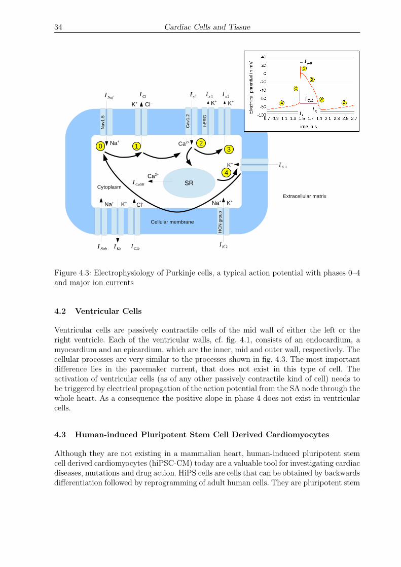
34 Cardiac Cells and Tissue
Figure 4.3: Electrophysiology of Purkinje cells, a typical action potential with phases 0–4and major ion currents
4.2 Ventricular Cells
Ventricular cells are passively contractile cells of the mid wall of either the left or theright ventricle. Each of the ventricular walls, cf. fig. 4.1, consists of an endocardium, amyocardium and an epicardium, which are the inner, mid and outer wall, respectively. Thecellular processes are very similar to the processes shown in fig. 4.3. The most importantdifference lies in the pacemaker current, that does not exist in this type of cell. Theactivation of ventricular cells (as of any other passively contractile kind of cell) needs tobe triggered by electrical propagation of the action potential from the SA node through thewhole heart. As a consequence the positive slope in phase 4 does not exist in ventricularcells.
4.3 Human-induced Pluripotent Stem Cell Derived Cardiomyocytes
Although they are not existing in a mammalian heart, human-induced pluripotent stemcell derived cardiomyocytes (hiPSC-CM) today are a valuable tool for investigating cardiacdiseases, mutations and drug action. HiPS cells are cells that can be obtained by backwardsdifferentiation followed by reprogramming of adult human cells. They are pluripotent stem

Cardiac Cells and Tissue 35
cells, meaning that they can be differentiated into any kind of cell existing in the humanbody. Since there are ethical concerns in performing experiments on native animal orhuman cells, the possibility of generating those cells from any cell, is brilliant and evenbrought the Nobel prize to Takahashi and Yamanaka [145].
When this method has been developed, of course it was questionable by what extentthe hiPSC-CM functionally resemble native human cells. It has been shown that thedifferentiation of human embryonic pluripotent stem cells (hePSC) leads to functionallysimilar adult cells. However, again there are ethical concerns in obtaining ePSC. Thus,hiPS cells are commonly used instead of hePSC. In fact, one major problem in using hiPScells is their immaturity or at least the unknown stage of maturity. This and the generalapplicability of experimental results obtained for hiPS cells to native human cells will beaddressed at many points within this thesis.
Despite the known and unknown differences between native and differentiated inducedcells they are commonly used because they are ethically acceptable. Thus they are cur-rently used as models for native human cardiomyocytes in the investigation of cardiac dis-eases (Liang and Du [91]), of drug action (Liang et al. [92], Mehta et al. [104])and the effect of mutations (Roden and Hong [128]).
4.4 Drug Action
The variety and the operating modes of known drugs are huge. Some drugs are actingsomewhere in the metabolism, thereby having some influence to the cardiovascular system.Some other drugs occupy proteins in the cell membrane thus limit the availability of thoseproteins to other drugs. Both operation modes are not part of the investigations in thisthesis. This work focuses on drugs that selectively influence specific ion channels withdifferent intensity and depending on their concentration. Those drugs can be inhibitoryand stimulating in the sense of blocking activation or inactivation gates (inhibition) orin the sense of accelerating the activation or inactivation of specific gates (stimulation).At the same time one drug can have an inhibitory behavior with respect to one gateand a stimulating behavior with respect to another gate with different potency. Bothactions change the action potential, thus change the beating force and the heart rate(beating frequency). In the following paragraphs the drugs and their ways of action thatare investigated within this thesis are explained.
4.4.1 Lidocaine
The common local anesthetic drug Lidocaine is clinically used as an antiarrhythmic drugfor emergency-treatment of ventricular arrhythmias. As a Class IB antiarrhythmic agent,it binds to fast sodium channels (Nav1.5) in their inactivated state, thereby inhibitingtheir activation. Its effectivity strongly rises with increased heart rate and therefore it hasa use-dependency. The block of fast sodium channels results in a decreased sodium influxINa during depolarization that subsequently causes a lowered inner calcium concentrationin ventricular myocytes during the action potential plateau due to the reverse mode of

36 Cardiac Cells and Tissue
the sodium-calcium-exchanger as reported by Saleh et al. [134]. Lidocaine thus lowersventricular contractile force.
Recent studies provide evidence for the inhibitory effect of Lidocaine on HCN channelswhich are assumed to be responsible for the pacemaker current thus the drug lowers theheart rate, Meng et al. [105].
4.4.2 Verapamil
Verapamil is a multi-ion-channel blocker classified as a class IV-antiarrhytmic agent. Incardiac tissue, this agent especially inhibits calcium ion influx through L-type calciumchannels (Cav1.2) during the early plateau phase as well as potassium ion efflux throughrapidly activating delayed rectifier potassium channels (hERG) during the late plateauand repolarization phases by dose-dependent blocking of the activation of the respec-tive channels. This causes a slower repolarization-rate that in turn leads to an actionpotential prolongation. The action potential prolongation leads to the expectation thatVerapamil induces a negative chronotropic effect, i.e. a reduction of the heart rate asfound by Arnold et al. [4]. The decreased calcium influx yields a negative inotropiceffect of Verapamil, i.e. a reduced beating force, since calcium ions play a major role inthe contraction process. Kramer et al. [87] reported that the drug additionally blocksfast sodium channels (Nav1.5), but with a very low potency.
4.4.3 Veratridine
Veratridine is a sodium channel toxin that solely prolongates the permeability of fastsodium channels (Nav1.5) by drug-induced inhibition of channel inactivation, resulting inan increased inner sodium ion concentration as found by Brill and Wasserstrom [20]and Honerjager and Reiter [74]. Saleh et al. [134] found that this consequentlytriggers an increase in intracellular calcium ions by stimulation of the sodium-calciumexchange and to an increased beating force. By an extension of the plateau phase, Vera-tridine additionally induces an action potential prolongation due to the lowered calciuminflux which results in a decreased beating frequency as found by Arnold et al. [4].
4.4.4 Bay K8644
In calf and guinea pig myocardial cells, Bay K8644 has been found to be a L-type cal-cium channel agonist which increases the calcium concentration in the cell thus it is apositively inotropic substance (Thomas et al. [149]). The drug not only increases theopen probability of the L-type calcium gates but also shifts the reversal potentials of theactivation and inactivation gates to more negative voltages and accelerates the decay ofthis channel (Chen et al. [28]).
Kang et al. [82] and Ji et al. [80] found that Bay K8644 does not show the channelactivating behavior in the case of hiPSC-CM and hePSC-CM. As this statement is notentirely true for all investigated cell cultures it is supposed that the lack of the effects instem cell-derived cardiomyocytes was due to an immaturity of the cells.

Mechanical and Electrophysiological Modeling of Cardiac Tissue 37
5 Mechanical and Electrophysiological Modeling of Cardiac Tis-
sue
From the modeling point of view cardiac tissue can be described by the three-elementmodel of Hill [69] that has been established in 1938 and is shown in fig. 5.1. The modelassumes a passive elastic element (PE) that is in parallel to a serial elastic (SE) elementwhich is in series with a contractile element (CE). Although within this thesis it is ap-plied to cardiac muscles only, Hill’s model is a general model that describes the passiveand active behavior of muscles, be they skeletal, smooth or cardiac muscles. The pas-sive element mainly corresponds to the extracellular matrix (ECM) that provides passivestiffness by collagen, elastin and other proteins. Besides its mechanical role the ECMplays a huge role in shaping cells, it contains ions and regulates ion diffusion necessary forproper cellular function and it serves as a biological scaffold for the cells (Humphrey [77],Alberts et al. [3]). Its constituent collagen is a protein that, in an unloaded environ-ment, is folded as can be seen in fig. 5.2. If the ECM, i.e. the tissue, is stretched, thecollagen proteins will unfold thus provide an anisotropic structure to the tissue and de-velop an increasing stress. The corresponding nonlinear relationship between stress andstrain can be seen in fig. 5.2 too. For small strains this relationship is highly flexible be-cause the protein is still unfolding but as soon as the collagen fibers are properly alignedthey produce an increasing stiffness.
Figure 5.1: Hill’s muscle model, Hill [69]Figure 5.2: Collagen structure at rest and instretching
In Hill’s model the active component that is in parallel to the passive element also producesa passive stress via the serial element. This element can be identified with the inherentelasticity provided by cross-bridges that form during contraction. Cross-bridges are builtby overlapping actin and myosin filaments, that, the more they overlap, increase thecontraction force. This passive contribution of the active element usually is neglectedbecause the passive stress that solely results from the contraction of the cells is rathersmall compared to the stress arising from the contractile component, i.e. the so-called

38 Mechanical and Electrophysiological Modeling of Cardiac Tissue
active stress.
In general the constitutive modeling of soft tissue is very flexible as can be seen for instanceregarding the structural mechanically motivated approach presented in Bol et al. [16].Therein a tetrahedral representative volume element has been created with truss elementslying on the edges of the tetrahedron. The volumetric stress contribution of the cardiactissue is computed based on the tetrahedral element whereas the passive stress arisingfrom the collagen fibers is reflected by the truss elements. The active stress component isalso incorporated via fiber-oriented truss elements.
Computationally oriented discussions of skeletal, smooth and cardiac muscle structureand more details on the interpretation of Hill’s model can be found in Spyrou [142].Although cardiac muscle is in the focus of this thesis, the very clear and concise practicalintroduction of Martins et al. [101] into the modeling of skeletal muscle using Hill’smodel is worth reading and nearly fully valid for cardiac muscle. The main differencebetween skeletal and cardiac muscle cells is that some of the latter are able to beatautonomously whereas the former cells need to be activated through the nerve system.
5.1 Active Stress Formulation
From the mechanical point of view there are the so-called active stress and the active strainformulations. The majority today employs the former one. Following the suggestions inthe cited literature, the active stress formulation is used herein but the active strainformulation is presented and discussed in the subsequent section. Therein the choice ofthe active stress formulation for the purposes of this thesis is justified.
The active stress formulation bases on the assumption that passive and active stressesoccur separately and both lead to deformation, thus the Cauchy stress
σ = σp + σa = 2J−1b∂Ψ(b)
∂b− pI + T (t, b)a⊗ a (5.1)
is split up into a passive part σp and an active part σa. In eq. (5.1), in the framework ofhyperelasticity, the passive stress is expressed via the strain energy Ψ and the hydrostaticpressure p. The active stress is given by a time- and strain-dependent scalar quantityT (t, b) that acts in a certain fiber direction a.
Both, models for the passive and active stress contributions of cardiac muscles, havebeen presented in the literature. A very famous and often employed model for σp
is a generalized version of the one shown in eq. (5.1). It has been proposed inHolzapfel and Ogden [73] and for incompressible soft biological tissue reads as
σp = 2∂Ψ
∂I1b+ 2
∂Ψ
∂I2(I1b− b2)− pI + 2
∂Ψ
∂I4aa⊗ a + 2
∂Ψ
∂I4ss⊗ s
+∂Ψ
∂I8as(a⊗ s+ s⊗ a) +
∂Ψ
∂I8an(a⊗ n+ n⊗ a) . (5.2)
Therein a sheet direction s that lies in the fiber plane and is normal to a and a normaldirection n that is normal to both have been introduced and respective invariants I∗ have

Mechanical and Electrophysiological Modeling of Cardiac Tissue 39
been formulated. This transversely isotropic stress formulation is much more sophisticatedthan the isotropic ones used herein but in turn it requires information about fiber orien-tation and the determination of many material parameters. It will become clear that forthe investigations in this thesis, the four terms in eq. (5.2) that are associated with theanisotropy can be ignored. Nevertheless it should be mentioned that such a complex stressformulation should be employed in whole heart simulations as the anisotropy significantlyinfluences the mechanical behavior.
The active stress contribution σa is detailed in sect. 5.4. The scalar T represents thecontractile stress and is determined by a system of ordinary differential equations (ODE)that comprises ODEs describing the cellular electrophysiology, the action potential and theso-called excitation-contraction coupling which is the actual electromechanical coupling.
5.2 Active Strain Formulation
The active strain formulation originates from Nardinocchi and Teresi [109] andCherubini et al. [29] who firstly proposed a multiplicative decomposition of the de-formation gradient
F = FeFa , (5.3)
for the analysis of passive and active deformation. The idea is that the elastic part ofthe deformation gradient Fe produces all the stress and that the active part Fa does notdeliver a stress contribution. The intermediate configuration that is created by Fa thus isconsidered to be virtual.
Very recently the active strain formulation has been applied to whole-heart simulations,like in Rossi et al. [131], Goktepe et al. [61] and Ruiz-Baier et al. [132] andto the simulation of isolated cardiomyocytes, cf. Ruiz-Baier et al. [133]. EspeciallyRossi et al. [131] theoretically compared multiple isotropic and anisotropic constitu-tive laws in the active stress and active strain frameworks. It comes out that in the smallstrain regime both are equivalent. In the finite strain regime though, they observe con-siderable differences in the deformation behavior that even become more severe when theconstitutive law becomes more complicated. The main reason for this can be seen bycomparing the first Piola-Kirchhoff stress in the active stress formulation
P = µF + Ta⊗ a0 (5.4)
and the active strain formulation
P = µ(1 + γa)F + µg(γa)a⊗ a0 (5.5)
for the very simple isotropic neo-Hookean material law. Interpreting γa as the relativedisplacement in the fiber axis one can clearly see that in eq. (5.5), in contrast to eq.(5.4), this relative displacement not only influences the anisotropic stress contributionbut also the isotropic one by the factor of (1 + γa). This basically means that an activecontraction influences the passive material response as well, i.e. it modifies the stiffnessof the material. The authors of the cited references leave open whether the active stress

40 Mechanical and Electrophysiological Modeling of Cardiac Tissue
or the active strain formulation is preferable. They suggest to conduct experiments thatlead to this decision but this is still an open issue.
As already pointed out, within this thesis the active stress formulation is applied. It ispreferable because it provides a disjunct split of passive and active stress contributionswhich is in accordance with the assumptions made in the experiments that serve for theparameterization of the employed models. It has to be mentioned though that the activestrain formulation might be able to cover microstructural effects at the macro-level thatwould be disregarded in the active stress formulation. However, it seems to be muchsimpler to regard passive and active stresses as fully disjunct, both experimental- andinterpretation-wise.
In the following sections the employed models for the passive stress are shown. The activestress contribution is in the main focus of this thesis and is discussed in very detail in thefollowing sections as well.
5.3 Modeling the Passive Component
In soft tissue biomechanics the passive stress is usually represented by a hyperelastic con-stitutive law. As already indicated in eq. (5.1), hyperelastic constitutive laws are definedby a strain energy function Ψ that represents the energy stored in the material. Ψ can beexpressed with the help of any strain measure and its derivative with respect to a certainstrain measure leads to the dual (conjugate) stress. Therefore the first Piola-Kirchhoffstress is given as
P =∂Ψ(F )
∂F(5.6)
and all other stress tensors can be derived using the transformation rules given in sect.2.1.2. In terms of this thesis the second Piola-Kirchhoff stress
S = F−1∂Ψ(F )
∂F(5.7)
and the Cauchy stress
σ = J−1∂Ψ(F )
∂FF T (5.8)
are of special interest. In general Ψ can be anisotropic, i.e. dependent on a number offiber families, which is often the case for biological soft tissues like muscles (usually onefiber family) or blood vessels (multiple fiber families).
A very common constraint on biological soft tissues is the incompressibility of the tissue,i.e. J = det(F ) = 1. This constraint can be introduced into the strain energy function bya Lagrangian multiplier p
Ψ = Ψ(F )− p(J − 1) , (5.9)
which is known to be the hydrostatic pressure. In the remainder of this work only incom-pressible and isotropic materials will be examined. Although cardiac tissue in general isanisotropic, it will be shown in sec. 6.1 (cf. fig. 6.3) that the herein investigated tissue is
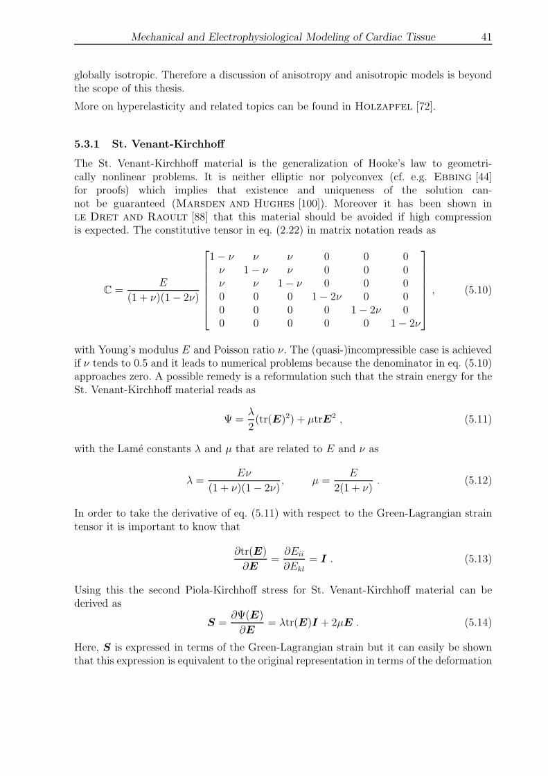
Mechanical and Electrophysiological Modeling of Cardiac Tissue 41
globally isotropic. Therefore a discussion of anisotropy and anisotropic models is beyondthe scope of this thesis.
More on hyperelasticity and related topics can be found in Holzapfel [72].
5.3.1 St. Venant-Kirchhoff
The St. Venant-Kirchhoff material is the generalization of Hooke’s law to geometri-cally nonlinear problems. It is neither elliptic nor polyconvex (cf. e.g. Ebbing [44]for proofs) which implies that existence and uniqueness of the solution can-not be guaranteed (Marsden and Hughes [100]). Moreover it has been shown inle Dret and Raoult [88] that this material should be avoided if high compressionis expected. The constitutive tensor in eq. (2.22) in matrix notation reads as
C =E
(1 + ν)(1 − 2ν)
1− ν ν ν 0 0 0ν 1− ν ν 0 0 0ν ν 1− ν 0 0 00 0 0 1− 2ν 0 00 0 0 0 1− 2ν 00 0 0 0 0 1− 2ν
, (5.10)
with Young’s modulus E and Poisson ratio ν. The (quasi-)incompressible case is achievedif ν tends to 0.5 and it leads to numerical problems because the denominator in eq. (5.10)approaches zero. A possible remedy is a reformulation such that the strain energy for theSt. Venant-Kirchhoff material reads as
Ψ =λ
2(tr(E)2) + µtrE2 , (5.11)
with the Lame constants λ and µ that are related to E and ν as
λ =Eν
(1 + ν)(1− 2ν), µ =
E
2(1 + ν). (5.12)
In order to take the derivative of eq. (5.11) with respect to the Green-Lagrangian straintensor it is important to know that
∂tr(E)
∂E=
∂Eii
∂Ekl
= I . (5.13)
Using this the second Piola-Kirchhoff stress for St. Venant-Kirchhoff material can bederived as
S =∂Ψ(E)
∂E= λtr(E)I + 2µE . (5.14)
Here, S is expressed in terms of the Green-Lagrangian strain but it can easily be shownthat this expression is equivalent to the original representation in terms of the deformation
42 Mechanical and Electrophysiological Modeling of Cardiac Tissue
gradient (cf. eq. (5.7)),
S =∂Ψ(E)
∂E=
∂Ψ(E)
∂F
∂F
∂E=
(∂E
∂F
)−1
∂Ψ(F )
∂F
=
(
1
2
∂(F TF − I
)
∂F
)−1
∂Ψ(F )
∂F
= F−1∂Ψ(F )
∂F. (5.15)
Herein the fact has been used that Ψ is defined in a way that it stays unchanged underrotation, i.e. Ψ(F ) = Ψ(RF ). Consequently all the different functions
Ψ(F ) = Ψ(U) = Ψ(V ) = Ψ(C) = Ψ(b) = Ψ(E) (5.16)
have the same value. This originates from the fact that with the polar decompositionsF = RU and F = V R of the deformation gradient tensor into an orthogonal rotationtensor R and a right and left stretch tensor U and V , respectively, the strain tensors
C = F TF = RUTRU = UTRTRU = UTU , (5.17)
b = FF T = V RV RT = V RRTV T = V V T and (5.18)
E =1
2(C − I) =
1
2(UTU − I) (5.19)
can be expressed independently of the rotation tensor. Intuitively it is clear that, in statics,rigid body rotation or translation does not cause any stress.
Taking the second derivative of Ψ with respect to E gives the constitutive tensor
C =∂S
∂E=
∂2Ψ(E)
∂E2= λI ⊗ I + 2µI ⊗ I = (λ+ 2µ)S , (5.20)
where the symmetric fourth-order tensor S has the components
Sijkl =1
2(δikδjl + δilδjk) (5.21)
and replaces the fourth-order identity tensor because E and S are symmetric. Equation(5.20) is equivalent to eq. (5.10). Both equations show that the St. Venant-Kirchhoffmaterial is isotropic and the material properties are strain-independent. Recapitulatingfig. 5.2, neither isotropy nor independence of strain can be assumed for cardiac tissue.Nevertheless this material model is useful for describing material in the linear regime.Regarding its limitations that already have been indicated above, the St.Venant-Kirchhoffmaterial model should only be used for boundary value problems with large rotations butsmall strains.
It can be shown that if a polyconvex or a quasiconvex strain energy density is requiredin the isotropic hyperelastic case, then the stress-strain relationship must be physicallynonlinear in the nonlinear strain measure.

Mechanical and Electrophysiological Modeling of Cardiac Tissue 43
5.3.2 Neo-Hookean
The Neo-Hookean material model is the simplest strain-dependent model and it can beviewed as a special case of the general Ogden model
Ψ = Ψ(λ1, λ2, λ3) =n∑
p=1
µp
αp
(λαp
1 + λαp
2 + λαp
3 − 3) , (5.22)
with the principal stretches λi, shear moduli µp and dimensionless parameters αp. SettingN = 1 and α1 = 2 leads to
Ψ(λ1, λ2, λ3) =µ1
2(λ2
1 + λ22 + λ2
3 − 3) = C10(I1 − 3) = Ψ(I1) , (5.23)
with I1(C) = tr(C) the first invariant of the right Cauchy-Green tensor.
This hyperelastic strain energy function in terms of the first invariant or the principalstretches is commonly used thus the passive stress contribution in eq. (5.1) has to bereformulated in terms of λi too. Using the identities derived in sect. 5.3.1 one gets
σp = 2J−1b∂Ψ(b)
∂b− pI = 2J−1V V T ∂Ψ(V )
∂V
∂V
∂b− pI
= 2J−1V V T ∂Ψ(V )
∂V
(∂b
∂V
)−1
− pI = J−1V V T ∂Ψ(V )
∂VV −1 − pI
= J−1V∂Ψ(V )
∂V− pI . (5.24)
The final step is to simply replace the left stretch tensor by its eigenvalues because σp
shall be expressed in its principal directions. The passive stress contribution then readsas
(σp)i = J−1λi
∂Ψ
∂λi
− pδii , (5.25)
with J = λ1λ2λ3. Of course there are many more different hyperelastic models for softtissues. Major benefits of the Neo-Hookean model are that it is polyconvex and that onlyone parameter C10 needs to be determined by parameter fitting. On the other hand morecomplex models allow a better approximation of the material curve if it has regions oflargely differing slopes, i.e. different degrees of nonlinearity. In the application that isinvestigated within this thesis the material behavior can accurately be approximated bythe Neo-Hookean material thus more complex models are not required.
The problems that are investigated in this thesis are modeled with either the St. Venant-Kirchhoff material for small deformation but large displacement or the Neo-Hookean ma-terial for large deformation problems.
5.4 Modeling the Contractile Component
The modeling of the contractile element in Hill’s model is most important for this thesis.This part of the model strongly depends on the type of muscle (skeletal, smooth or cardiac)

44 Mechanical and Electrophysiological Modeling of Cardiac Tissue
and on the cell type because the action potentials of different cells in the heart, like AVcells, SA cells, Purkinje cells or ventricular cells differ significantly. It has already beenexplained that the main driver for the contractility of any cardiac cell is the concentrationof free inner calcium.
In standard tissue models one uses an electrophysiological model of a specific cell type inorder to create an action potential and to compute the free inner calcium concentration[Ca2+]i, which then serves as input for the computation of the active stress contributionσa in eq. (5.1).
There are different ways of modeling cell electrophysiology, cf. Ay and Arnosti [5], butmost commonly the electrophysiological processes across the cell membrane (cf. fig. 4.3)are modeled by a system of ordinary differential equations in the form of
dVm
dt=
1
Cm
(
Istim −M∑
i=1
Ii(g1, g2, ..., gMi)
)
(5.26)
dgj(Vm)
dt= α+
j (Vm)(1− gj) + α−
j (Vm)gj , (5.27)
where Vm is the cell membrane potential, Cm is the electrical capacitance of the cellmembrane, Istim is an external (potentially zero) electrical stimulus, Ii are ionic currentsand M is the total number of ionic currents in the model. Each current depends on Mi
(usually one or two) gate variables gj that control the opening and closure of the ionicchannel i where ions diffuse through. α+
j and α−
j are experimentally determined openingand closure rates of the respective gate. They depend on Vm, i.e. for each gate there arethreshold values for the membrane potential that determine the opening and closure ofthe respective gate.
The membrane potential itself is determined by the difference of an externally applied cur-rent Istim and the ionic currents that are governed by the gates. The idea for this very gen-eral electrophysiological model for a single cell goes back to Hodgkin and Huxley [71].Since then numerous special single-cell models have been developed based on an immenseamount of experiments to determine the electrical, mechanical and electromechanicalproperties of cells and single ion channels. As the knowledge of cellular processes is stillincomplete but continuously increasing the quantification of the properties is work inprogress. Extensive overviews over electrophysiological cell models of different mammalianand human cell types that also have been used to study the electrical propagation in car-diac tissues are provided by Fenton and Cherry [49] and Nickerson [115]. Thosemodels have different complexity, ranging from two variables to very complex modelsthat consist of up to 60 variables. They are too numerous to name them all, i.e. only themodels that have been used in this work will be explained.
As already indicated in Ruiz-Baier et al. [132], currently there is no model that prop-erly builds the bridge between the cell and tissue scales by means of homogenization.Usually the micro-scale effects are directly transmitted to the macro-scale, i.e. concerningthe contractile behavior, the tissue is treated as if it would consist of cells only, with-out an extracellular matrix. Those models are referred to as monodomain models. Inorder to benefit from the detailed data on the cell level in tissue analysis, a switchover

Mechanical and Electrophysiological Modeling of Cardiac Tissue 45
to bidomain models is important. The theoretical background of which can be found inNobile et al. [119].
5.4.1 Different Scales
At first one has to distinct between the modeling on different scales. There are approachesof modeling optical effects on the Angstrom to the nano-scale to achieve realistic multi-scale behavior of the heart. Chemical processes like diffusion of ions through the ionchannels of the cell take place on the nano- to the micro-scale. Within this thesis chemicalprocesses are modeled at the cell level (micro-scale) ignoring the local effects that takeplace at the nano-scale. The chemical and electrophysiological cellular processes are muchfaster than the mechanical response of the tissue. Therefore the tissue which consists ofmillions of cells is not only modeled on a coarser length scale but also on a coarser timescale. Crossing the scales is rather simple in the model developed herein.
An even larger scale is the organ itself. For basic investigations like the simulation ofdrug action on a tissue this scale is too large regarding the fact that cellular processes arenot entirely understood and that corresponding models are under current development.Some research has been done in the simulation of the mechanics and the propagation ofthe electrical potential through the human heart including mechano-electrical feedback,likeGoktepe and Kuhl [59],Hunter et al. [79] and Smith et al. [141] but mostlywithout crossing the scales to the cell level. An exception to that is the recently proposedframework byGoktepe et al. [61] that allows for internal ordinary differential equationsystems describing the cellular electrophysiology.
Computational models at the tissue and organ level are often chosen for the investigationof the electromechanics of the whole heart, i.e. when the organ deformation, the electricalconduction system or mechano-electrical effects are of interest. Models at the cellular levelare employed when individual ion currents, specific gates or proteins, the cellular actionpotential or the cellular communication via gap junctions are studied. Cellular models areoften used for the computational assessment of single cells, cell clusters or even tissue, likein the present case. Fully bridging the scales from the cellular level up to the organ levelis very challenging and is discussed in the outlook section 9 as a current research topic.
5.4.2 Modeling Drug Action
Before starting to explain the chosen electrophysiological models, the general way of mod-eling drug action within the Hodgkin-Huxley framework shall be clarified.
Different drugs typically have different effects on the membrane potential. First of all, adrug may change the activation or inactivation gate of a certain channel or possibly multi-ple gates in a varying amount. The two basic effects that are investigated are the blockingand the stimulation of the activation or the inactivation of a certain gate, respectively.The modeling approaches of both are different and strongly depend on the data that istaken from experiments.
46 Mechanical and Electrophysiological Modeling of Cardiac Tissue
5.4.2.1 Blocking Drugs In patch clamp experiments one quantifies an IC50 valuewhich is the half-blocking concentration of a drug with respect to a certain gate. In otherwords the IC50 value is the concentration of the drug that is needed to slow down theion flux through the respective channel by 50%. Knowing the constant IC50 value thatfor instance can be taken from literature and the actually applied drug concentrationD, Obiol-Pardo et al. [121] simply introduce a scaling factor into the respective gatedifferential equation (5.27)
dgj(Vm; ICd50, D
d)
dt=
1
1 + Dd
ICd50
(α+j (Vm)(1− gj) + α−
j (Vm)gj). (5.28)
Obviously this scaling factor equals 0.5 (half-blocking) if Dd = ICd50, where the upper
index d indicates a specific drug. One has to be very careful in searching appropriate IC50
values. This experimentally determined parameter depends on the drug, the ion channel,the cell type, the cell environment, stretch, etc. Depending on the numerous influences,values from different publications that seem to be determined in a similar environmentoften lie in a wide range.
5.4.2.2 Stimulating Drugs Stimulating effects of drugs are modeled in a dif-ferent way. Experimentally one observes that either the opening rate α+
j or the closurerate α−
j or both are affected by a drug. Those rates are often defined with respect to athreshold potential. Thus if Vm reaches the threshold potential the gate opens. In patchclamp experiments one can measure a shift of a test action potential with respect to thedrug concentration. The determined potential shifts ∆V +
j and ∆V −
j are added in order tomodify the threshold. Intuitively it is clear that if the gate becomes activated at a lowerpotential, i.e. it opens earlier, and if the inactivation stays unchanged, then the gate willbe in the open state for a longer time, which has a positive effect on the ion flux. Thesame is true for unchanged activation but later inactivation (at higher potentials). Thegate differential equation including the potential shift is introduced as
dgj(Vm)
dt= α+
j (Vm +∆V +j )(1− gj) + α−
j (Vm +∆V −
j )gj . (5.29)
Depending on the affected ion channel, a potential shift might result in a changing beatingforce or beating frequency of the cell. Of course both effects can be seen at the same time,especially if the drug acts on a specific calcium channel and on a specific potassiumchannel, the latter of which often is called the pacemaker channel. Also, there is the wellknown staircase effect that reveals a positive proportionality of cell beating force withrespect to the beating frequency.
From a modeling point of view one has to be very cautious about how the drug is supposedto change the cellular processes and where in the model this effect can be introduced andabout the experimentally determined potential shifts that again underlie uncertainties.The application of multiple drugs at the same time with opposing effects is possible ingeneral but has not been investigated in here.

Mechanical and Electrophysiological Modeling of Cardiac Tissue 47
5.4.3 Electrophysiological Models
In order to understand how the choice of the proper cell models for the purposes of thisthesis have been made, it is necessary to provide an overview about the currently existingmodels. Models for SA cells and ventricular cells are in the focus because those are theinvestigated cell types.
The first model that has been implemented during this work is the Fenton-Karma modelFenton and Karma [48] for ventricular cells representing a fast-inward, a slow-inwardand a slow-outward current. Each of those three currents represents an assembly of anumber of ion currents. In the view of simulation of drug action the level of detail ofthe Fenton-Karma model is not sufficient because drugs selectively act on ion channelsand in order to simulate this appropriately the respective ion channels need to have aseparate representation. Moreover this model represents ventricular cells which are notautonomously beating but which need a trigger from outside. In the human heart as wellas in the investigated tissues the stimulus originates from nodal cells, like SA cells.
For the sake of simplicity, models have been chosen that do not have much more than20 unknowns in total. For the investigations in this thesis a higher degree of detail is notnecessary and may be even confusing. It is already difficult to find reliable experimentaldata concerning action potentials of and drug action on different type of cells. The unre-liability originates from different factors like the cell environment, species, uncertainty ofcell type, the influence of the respective experimental setup and whether the experimentsare performed on the level of single ion channels, single cells, tissues or organs. Especiallythe herein investigated human-induced pluripotent stem cells (hiPSC) show considerablydifferent behavior depending on those and other factors because all over the world theyhave a different origin. Given the fact that it is very difficult to select appropriate datafor hiPS cells from the literature, it is important to keep the models simple in order toprovide a certain range of applicable data instead of not being able to find any data.
Besides those concerns there is another one that has already been mentioned: the differ-ence between hiPS cells and native human cells thus the applicability of results obtainedwith hiPS cells. Although they provide a good and promising basis for ethically beneficialexperiments they are functionally different or immature. Recent experimental and simula-tion studies like Ji et al. [80] and Hu et al. [75], respectively, show that currently it isdangerous trying to transfer hiPSC results to native cells as largely significant functionaldifferences can be seen between different cell lines and even within one cell line.
In order to understand the basic properties of self-contractile cell models, two modelsfor Purkinje fiber cells have been implemented: the Noble model, Noble [120] and theMcAllister-Noble-Tsien (MNT) model, McAllister et al. [103]. The former one againis a very simple model having only four variables and therefore is not well-suited for thesimulation of drug action. The MNT model was the first model that has been used hereinto simulate self-contractile tissue and drug action.
During data evaluation it appeared that the calcium dynamics needed to be simulatedin much more detail than it has been done in this first setup. In addition to that theinvestigated tissues consist of multiple different cell types: nodal, atrial and ventricular CM

48 Mechanical and Electrophysiological Modeling of Cardiac Tissue
as well as fibroblasts. Taking this into account two more recent models have been selectedand implemented. The model of Stewart et al. [143] is a Purkinje fiber model, just likethe MNT model. This model has been chosen because it models the calcium dynamics inmuch more detail and because it is parameterized based on data of human Purkinje fibercells in contrast to the MNT model that is mostly based on rabbit and canine data. In thefinite element model the Stewart model serves as the pacemaker without a geometricalrepresentation. In turn, the human ventricular model of ten Tusscher et al. [147] andten Tusscher and Panfilov [146] (TT) is applied everywhere to simulate the cardiacaction potential.
Choosing a Purkinje fiber model instead of a proper nodal model seems to be arbitrary.During the work on the thesis the MNTmodel for Purkinje cells has been chosen because ofits limited number of ionic currents such that basic electrophysiological effects are clearlyrepresented. Later, when a human model was required, the differences to the MNT modelshould be as little as possible in order to be able to keep track of the changes in theresults. Thus, in order to keep the cell type, a consequent choice was the Stewart modelfor human Purkinje cells. It will be pointed out in sections 5.4.5 and 9.2.2 that humanSA models have been chosen for further investigations that extend this thesis.
The three models, MNT, Stewart and TT, that have been used in the simulations areexplained in the following paragraphs.
5.4.3.1 McAllister-Noble-Tsien The MNT model proposed inMcAllister et al. [103] consists of ten variables and therefore it is sufficientlycomplex to appropriately simulate drug action but not too complex to be confusingconcerning the adjustable parameters. Here, the equations and parameters of the originalmodel are shown. If different parameters have been used (Nickerson [115] shows someminor differences) it is explicitly stated. The following equations form a model for thecellular processes that have been described with the help of fig. 4.3 and the actionpotential one can compute from this model is shown in fig. 5.3. The different phases ofthe AP have been explained in sect. 4.1 and it shall be emphasized here that one canclearly observe a rising of the AP before depolarization and after the beat. Consequently,the model will reach its threshold potential on its own and beats with a frequency ofabout 0.77 s−1.
Disregarding the units in eqs. (5.30–5.38) for compactness, the ion currents in the MNT
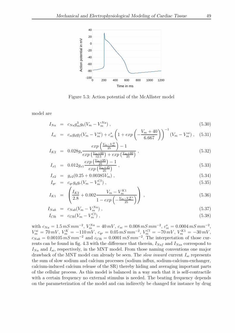
Mechanical and Electrophysiological Modeling of Cardiac Tissue 49
Figure 5.3: Action potential of the McAllister model
model are
INa = cNag3mgh(Vm − V Na
m ) , (5.30)
Isi = csigdgf(Vm − V sim ) + c∗si
(
1 + exp
(
−Vm + 40
6.667
))−1
(Vm − V sim ) , (5.31)
IK2 = 0.028gsexp
(Vm−V K
m
25
)
− 1
exp(Vm+6012.5
)+ exp
(Vm+60
25
) , (5.32)
Ix1 = 0.012gx1exp
(Vm+95
25
)− 1
exp(Vm+45
25
) , (5.33)
Ix2 = gx2(0.25 + 0.00385Vm) , (5.34)
Iqr = cqrgqgr(Vm − V Clm ) , (5.35)
IK1 =
IK2
2.8+ 0.002
Vm − V K1m
1− exp(
−Vm−V K1m
25
)
, (5.36)
INab = cNab(Vm − V Nam ) , (5.37)
IClb = cClb(Vm − V Clm ) , (5.38)
with cNa = 1.5mSmm−2, V Nam = 40mV , csi = 0.008mSmm−2, c∗si = 0.0004mSmm−2,
V sim = 70mV , V K
m = −110mV , cqr = 0.05mSmm−2, V Clm = −70mV , V K1
m = −30mV ,cNab = 0.00105mSmm−2 and cClb = 0.0001mSmm−2. The interpretation of those cur-rents can be found in fig. 4.3 with the difference that therein, INaf and INas correspond toINa and Isi, respectively, in the MNT model. From those naming conventions one majordrawback of the MNT model can already be seen. The slow inward current Isi representsthe sum of slow sodium and calcium processes (sodium influx, sodium-calcium-exchanger,calcium-induced calcium release of the SR) thereby hiding and averaging important partsof the cellular process. As this model is balanced in a way such that it is self-contractilewith a certain frequency no external stimulus is needed. The beating frequency dependson the parameterization of the model and can indirectly be changed for instance by drug
50 Mechanical and Electrophysiological Modeling of Cardiac Tissue
application or other parameter adjustments. By setting Cm = 0.1µF mm−2 the currents(5.30)–(5.38) determine the time course of the membrane potential, eq. (5.26).
To complete the model the activation and inactivation parameters of the nine gates ofthis model are shown. Again, the units are ommited:
α+m =
Vm + 47
1− exp(−Vm+47
10
) α−
m = 9.86exp
(
−Vm + 47
17.86
)
(5.39)
α+h = 1.13 · 10−7exp
(
−Vm + 10
5.43
)
α−
h = 2.5
(
1 + exp
(
−Vm + 10
12.2
))−1
(5.40)
α+d = 0.002
Vm + 40
1− exp(−Vm+40
10
) α−
d = 0.02exp
(
−Vm + 40
11.26
)
(5.41)
α+f = 0.00253exp
(
−Vm + 26
25
)
α−
f = 0.02
(
1 + exp
(
−Vm + 26
11.49
))−1
(5.42)
α+q = 0.008
Vm
1− exp(−Vm
10
) α−
q = 0.08exp
(
−Vm
11.26
)
(5.43)
α+r = 2.08 · 10−5exp
(
−Vm + 26
25
)
α−
r = 0.02
(
1 + exp
(
−Vm + 26
11.49
))−1
(5.44)
α+s = 0.001
Vm + 52
1− exp(−Vm+52
5
) α−
s = 5 · 10−5exp
(
−Vm + 52
14.93
)
(5.45)
α+x1 = 5 · 10−4 exp
(Vm+5012.1
)
1 + exp(Vm+5017.5
) α−
x1 = 0.0013exp
(−Vm+20
16.67
)
1 + exp(−Vm+20
25
) (5.46)
α+x2 = 1.27 · 10−4
(
1 + exp
(
−Vm + 19
5
))−1
α−
x2 = 3 · 10−4 exp(−Vm+20
16.67
)
1 + exp(−Vm+20
25
) (5.47)
Each gate is expressed in the form of eq. (5.27). In order to couple this model to the modelsof contraction described in sect. 5.4.4, another ordinary differential equation needs to beintroduced that determines the inner calcium concentration. In the model of contractionthe calcium concentration at a certain time serves as direct input. Unlike other models theMNTmodel does not provide such a differential equation but inBeeler and Reuter [9]the differential equation
∂[Ca2+]i∂t
= −1.848 · 10−4Isi + 0.07(10−4 − [Ca2+]i) (5.48)
has been proposed that uses Isi as input. Here it has already been scaled to a minimumcalcium concentration of 0.1µM and a maximum calcium concentration of 1µM. Anyother scaling is also possible depending on the cell type to model.
5.4.3.2 ten Tusscher et al. This model of human ventricular cells consists of 17variables that are explained in detail in ten Tusscher and Panfilov [146]. The time

Mechanical and Electrophysiological Modeling of Cardiac Tissue 51
course of the membrane potential is determined by a total of 12 ion currents and a possi-ble stimulus. As ten Tusscher et al. [147] and ten Tusscher and Panfilov [146]are very detailed, within this thesis only some ion currents and some specific gates areexplained depending on whether they are influenced by a drug. However, all the differen-tial equations are shown here because they slightly differ from those shown in the citedpapers due to minor mistakes that have been corrected in Niederer and Smith [116].Each of the gate differential equations is written in the form
∂gj(Vm)
∂t=
ginfj − gj
τgj, (5.49)
with time constants
τgj = α+gjα−
gj+ β−
gj(5.50)
for most of the gates except for the j- and h-gates for which
τgj =1
α+gj+ α−
gj
. (5.51)
Avoiding the units in the equations of this section as well, the activation and inactivationconstants α+
gj, α−
gjand β−
gjfor each gate are given as follows
α+m =
1
1 + exp(−Vm+60
5
) α−
m =0.1
1 + exp(Vm+35
5
) +0.1
1 + exp(Vm−50200
)
β−
m = 0 minf =1
(1 + exp
(−Vm+56.86
9.03
))2
α+d =
1.4
1 + exp(−Vm+35
13
) + 0.25 α−
d =1.4
1 + exp(Vm+5
5
)
β−
d =1
1 + exp(50−Vm
20
) dinf =1
1 + exp(−Vm+8
7.53
)
α+x1 =
450
1 + exp(−Vm+45
10
) α−
x1 =6
1 + exp(Vm+3011.5
)
β−
x1 = 0 x1inf =1
1 + exp(−Vm+26
7
)
α+x2 =
3
1 + exp(−Vm+60
20
) α−
x2 =1.12
1 + exp(Vm−60
20
)
β−
x2 = 0 x2inf =1
1 + exp(Vm+88
24
)
α+xs =
1400√
1 + exp(5−Vm
14
) α−
xs =1
1 + exp(Vm−35
15
)
β−
xs = 80 xsinf =1
1 + exp(−Vm+5
14
)

52 Mechanical and Electrophysiological Modeling of Cardiac Tissue
α+h =
0.057exp
(−Vm+80
6.8
), Vm < −40
0, else
α−
h =
2.7exp(0.079Vm) + 310000exp(0.3485Vm), Vm < −400.77
0.13(1+exp(−Vm+10.6611.1 ))
, else
hinf =1
(1 + exp
(Vm+71.55
7.43
))2 β−
h = 0
α+j ==
(−25428exp(0.2444Vm)−6.948·10−6exp(−0.04391Vm))(Vm+37.78)
(1+exp(0.311(Vm+79.23)))−1 , Vm < −40
0, else
α−
j =
0.02424exp(−0.01052Vm)
1+exp(−0.1378(Vm+40.14)), Vm < −40
0.6exp(0.057Vm)1+exp(−0.1(Vm+32))
, else
jinf =1
(1 + exp
(Vm+71.55
7.43
))2 β−
j = 0 .
For the remaining f -, f2-, fCaSS-, s- and r-gates the inferior values and the time constantsare given as follows
τf = 1102.5exp
(
−(Vm + 27)2
225
)
+200
1 + exp(13−Vm
10
) +180
1 + exp(Vm+30
10
) + 20
finf =1
1 + exp(Vm+20
7
)
τf2 = 562exp
(
−(Vm + 27)2
240
)
+31
1 + exp(25−Vm
10
) +80
1 + exp(Vm+30
10
)
f inf2 =
0.67
1 + exp(Vm+35
7
) + 0.33
τfCaSS=
80
1 +(CaSS
0.05
)2 + 2
f infCaSS =
0.6
1 +(CaSS
0.05
)2 + 0.4
τs = 85exp
(
−(Vm + 45)2
320
)
+5
1 + exp(Vm−205
)+ 3
sinf =1
1 + exp(Vm+205
)
τr = 9.5exp
(
−(Vm + 40)2
1800
)
+ 0.8
rinf =1
1 + exp(20−Vm
6).
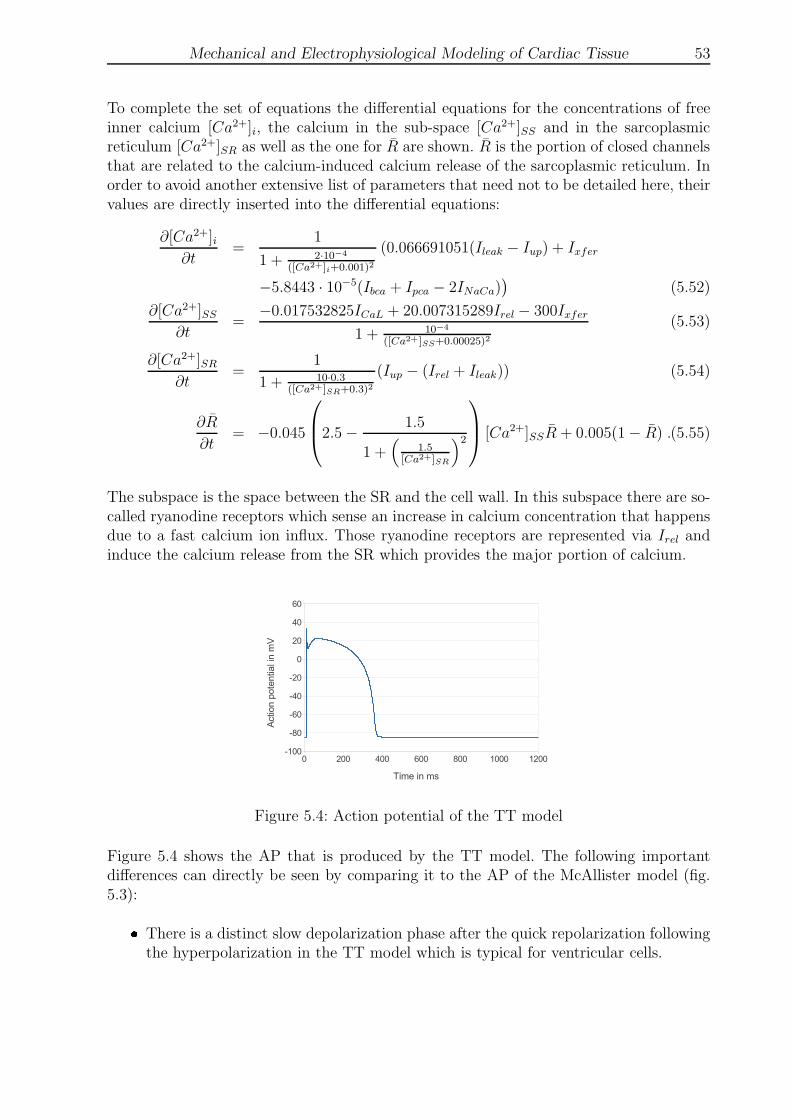
Mechanical and Electrophysiological Modeling of Cardiac Tissue 53
To complete the set of equations the differential equations for the concentrations of freeinner calcium [Ca2+]i, the calcium in the sub-space [Ca2+]SS and in the sarcoplasmicreticulum [Ca2+]SR as well as the one for R are shown. R is the portion of closed channelsthat are related to the calcium-induced calcium release of the sarcoplasmic reticulum. Inorder to avoid another extensive list of parameters that need not to be detailed here, theirvalues are directly inserted into the differential equations:
∂[Ca2+]i∂t
=1
1 + 2·10−4
([Ca2+]i+0.001)2
(0.066691051(Ileak − Iup) + Ixfer
−5.8443 · 10−5(Ibca + Ipca − 2INaCa))
(5.52)
∂[Ca2+]SS∂t
=−0.017532825ICaL + 20.007315289Irel − 300Ixfer
1 + 10−4
([Ca2+]SS+0.00025)2
(5.53)
∂[Ca2+]SR∂t
=1
1 + 10·0.3([Ca2+]SR+0.3)2
(Iup − (Irel + Ileak)) (5.54)
∂R
∂t= −0.045
2.5−
1.5
1 +(
1.5[Ca2+]SR
)2
[Ca2+]SSR + 0.005(1− R) .(5.55)
The subspace is the space between the SR and the cell wall. In this subspace there are so-called ryanodine receptors which sense an increase in calcium concentration that happensdue to a fast calcium ion influx. Those ryanodine receptors are represented via Irel andinduce the calcium release from the SR which provides the major portion of calcium.
Figure 5.4: Action potential of the TT model
Figure 5.4 shows the AP that is produced by the TT model. The following importantdifferences can directly be seen by comparing it to the AP of the McAllister model (fig.5.3):
There is a distinct slow depolarization phase after the quick repolarization followingthe hyperpolarization in the TT model which is typical for ventricular cells.

54 Mechanical and Electrophysiological Modeling of Cardiac Tissue
The AP of the TT model is more bulgy which is typical for ventricular cells andatypical for nodal or Purkinje cells.
The TT model does not show a rise of the AP during the resting state. It represents aventricular cell thus it needs to be paced from outside by either an external stimulusor another cellular model that provides one.
5.4.3.3 Stewart The Stewart model resembles the TT model in many parts. Themost important difference between those models is the introduction of a so-called funnycurrent
If = If,K + If,Na , (5.56)
that is responsible for the repolarization phase and serves as the pacemaker. It is drivenby two sub-currents that result from potassium and sodium ion fluxes, respectively. Theyare governed by the membrane potential and a newly introduced gate y and read as
If,K = cf,Ky(Vm − EK) (5.57)
If,Na = cf,Nay(Vm − ENa) , (5.58)
with conductivities cf,K = 0.0234346nSpF−1 and cf,Na = 0.0145654nSpF−1 and equi-librium potentials Ef,K = −86.3596773mV and Ef,Na = 74.51577033mV . The y gate isdefined by
α+y = exp(−2.9 − 0.04Vm) α−
y = exp(3.6 + 0.11Vm) (5.59)
τy =4000
α+y + α−
y
yinf =1
1 + exp(Vm+80.6
6.8
) . (5.60)
Compared to the TT model there are slight changes in the r- and s-gates and in thecurrents to account for human Purkinje fiber cells instead of ventricular cells. Furtherdetails of this model can be found in Stewart et al. [143].
Figure 5.5: Action potential of the Stewart model
Figure 5.5 shows the AP of the Stewart model and again some differences become apparentwith respect to the other two models:

Mechanical and Electrophysiological Modeling of Cardiac Tissue 55
The AP shape looks like a mixture of both previous models. This is due to the factthat the Stewart model just alters the TT model and adds the funny current thatprovides Purkinje cell characteristics.
The AP duration is a little bit shorter than in the McAllister model because theStewart model is parameterized for human rather than for rodent Purkinje cells.
The beating frequency of both, the McAllister and the Stewart model, is about0.77 s−1.
5.4.4 Models of Contraction
In this section suitable models for the description of the active stress component in eq.(5.1) are explained and evaluated. Therein the scalar quantity T (t, b) depends on thetime and the left Cauchy-Green tensor b. Current models that describe the active stressof cardiac muscles are formulated one-dimensionally with respect to the stretch λ in fiberdirection. To the authors knowledge there is no two-dimensional model of the contractilestress. Therefore, within this thesis, T (t, b) is simplified to T (t, λ1) = T (t, λ2) = T (t, λ),such that the principal stretches λ1 and λ2 are assumed to be equal. This assumptionis valid because the circular specimen to be studied is in an equibiaxial strain state.Moreover the specimen is isotropic (cf. sec. 6.1), thus principal stretches are taken for the’fiber stretches’.
T (t, λ) implicitly depends on [Ca2+]i. In the original publications that present the follow-ing models, a time course of [Ca2+]i is usually prescribed. As in this work the calciumconcentration in the cytoplasm is determined by a model of cell electrophysiology, [Ca2+]iis the interface between the models of cell electrophysiology and of mechanical stressdevelopment.
5.4.4.1 Hunter-McCulloch-ter Keurs The Hunter-McCulloch-ter Keursmodel (HMT) proposed in Hunter et al. [78] was the first choice because of itsrelative simplicity. In its original version all model parameters have been taken fromanimal testing. The application to human cardiac cells is questionable but as experimentaldata for humans were and are quite rare this model is still one of the best choices. Animproved version of this model including some model parameters that then have beenderived from human cardiac cells is given in the next paragraph.
The HMT model assumes the active stress to be determined by
T (t, λ, [Ca2+]i) = Tref(1 + β0(λ− 1))z(t, λ, [Ca2+]i), (5.61)
with β0 being a measure of how cooperatively neighboring myofilaments interact, thereference tension of a cell Tref and z being an activation variable. If there is no interactionof neighboring myofilaments, β0 = 1 and the length-dependent tension development wouldresult from the changing myofilament overlap only.
The activation variable z represents the tropomyosin kinetics that result from the bindingof [Ca2+]i to troponin C (TnC). With 0 ≤ z ≤ 1 it equals the portion of available actin
56 Mechanical and Electrophysiological Modeling of Cardiac Tissue
sites. The system of ordinary differential equations to describe the activation state of thecardiac muscle is given as
∂z
∂t= α0
(([Ca2+]b[Ca2+]50b
)n
(1− z)− z
)
(5.62)
∂Cab∂t
= ρ0[Ca2+]i([Ca2+]maxb − [Ca2+]b)− ρ1
(
1−Tcb
γTref
)
[Ca2+]b , (5.63)
with the concentration of bound calcium Cab, the half maximal calcium concentration
[Ca2+]50i = 106−(p[Ca2+]50refi (1+β2(λ−1))) (5.64)
and the Hill coefficientn = nref(1 + β1(λ− 1)) . (5.65)
An active crossbridge binding (Tcb > 0) slows down the unbinding and it can even stop theunbinding when, at maximum, Tcb = γTref . Due to a very little influence and to reducethe model complexity, crossbridge binding is neglected here, thus one chooses Tcb = 0.
The time course of [Ca2+]i is given by the electrophysiological model. A summary anddescription of the model parameters as well as their values is given in table 5.1. Moredetails about this model and explanations where the experimental data have been takenfrom is given in Hunter et al. [78].
Table 5.1: Parameters of the original HMT model
Parameter Value Interpretationρ0 0.1 µM−1ms−1 binding rate TnC-Ca2+
ρ1 0.163 ms−1 unbinding rate TnC-Ca2+
γ 2.6 effect of tension on ρ1[Ca2+]max
b 2.26 µM saturation [Ca2+]bα0 0.002 ms−1 activation and inactivation rate (actin sites)nref 6.9 reference Hill coefficient for cooperativity of actin sites
p[Ca2+]50refi 6.2 exponential reference half-maximal [Ca2+]iTref 100 kPa tension at resting SLβ0 1.45 tension-length dependency of Tβ1 1.95 tension-length dependency of nβ2 0.31 tension-length dependency of [Ca2+]50b
It has to be emphasized that the reference tension of a cell, Tref = 100kPa in table 5.1does not have any relevance as in this thesis it is determined by a parameter fitting. Thefitted value might be differently interpreted as a reference tension of the overall tissue andtherefore it is four to five orders of magnitude lower.
5.4.4.2 Niederer et al. The Niederer-Hunter-Smith model (NHS) can be foundin Niederer et al. [117]. It improves the HMT model by adding more details and byfitting some of the parameters to human cardiac cells. One major difference betweenthe two models is the introduction of the parameter zmax that represents the maximum
Mechanical and Electrophysiological Modeling of Cardiac Tissue 57
portion of available actin binding sites. It is incorporated because it is assumed that evenat full activation not all actin sites are available. The muscle tension then reads as
T = Tref(1 + β0(λ− 1))z
zmax
. (5.66)
The differential equation describing the concentration of bound calcium again is eq. (5.63)but z is now determined by
∂z
∂t= α0
([Ca2+]b[Ca2+]50b
)n
(1− z)− αr1z − αr2znr
znr +Knr
Z
, (5.67)
thus binding as well as slow and fast unbinding processes of calcium to and from TnC areseparated. The algebraic equations to compute the maximum portion of available actinsites and the half-maximal concentrations of bound and free inner calcium, respectively,are
zmax =
α0([Ca2+]maxb )
n
([Ca2+]50b )
n −K2
αr1 +K1 +α0([Ca2+]max
b )n
([Ca2+]50b )
n
(5.68)
K1 =αr2z
nr−1p nrK
nr
Z(znrp +Knr
Z
)2 (5.69)
K2 = αr2
znrp
znrp +Knr
Z
(
1−nrK
nr
Z
znrp +Knr
Z
)
(5.70)
[Ca2+]50b = [Ca2+]maxb
[Ca2+]50i
[Ca2+]50i +ρref1
ρ0
(
1− 0.5(1+β0(λ−1))γ
) (5.71)
[Ca2+]50i = [Ca2+]50refi (1 + β1(λ− 1)) . (5.72)
The original parameter values are given in table 5.2. Again, Tref will be re-placed by an experimentally determined value. In Niederer and Smith [116] andWeise and Panfilov [156] this model has been used to simulate human cardiac tis-sue. Therein the myocyte relaxation rates αr1 = 0.01s−1 and αr2 = 0.025s−1 are modifiedin order to achieve a faster relaxation. Also Tref = 125kPa and p[Ca2+]50refi = 6.5 havebeen adopted.
The cross-bridge binding kinetics, i.e. the history-dependent relaxation that has beenproposed in the NHS model have been implemented as well but as this does not affectthe results too much, it is not detailed here but can be found in Niederer et al. [117].
5.4.5 Excitation-Contraction Coupling
The presented HMT and NHS models require the time course of free intra-cellular calciumas input. In its original version the MNT model does not provide a differential equationfor [Ca2+]i thus the coupling differential equation (5.48) needs to be implemented.

58 Mechanical and Electrophysiological Modeling of Cardiac Tissue
Table 5.2: Parameters of the original NHS model
Parameter Value Interpretationρ0 0.1 µM−1ms−1 binding rate TnC-Ca2+
ρ1 0.2 ms−1 reference unbinding rate TnC-Ca2+
γ 2 effect of tension on ρ1[Ca2+]max
b 70 µM saturation [Ca2+]bα0 0.008 ms−1 activation rate (actin sites)αr1 0.002 ms−1 slow relaxation rate (actin sites)αr2 0.00175 ms−1 fast relaxation rate (actin sites)n 3 Hill coefficient for cooperativity of actin sitesKZ 0.15 fitted relaxation parameter (actin sites)nr 3 fitted relaxation parameter (actin sites)zp 0.85 point of Taylor expansion for zβ1 -4 SL dependency of [Ca2+]50i[Ca2+]50refi 1.05 µM reference half-maximal [Ca2+]iTref 56.2 kPa tension at resting SLβ0 4.9 tension-length dependency of T
The combined HMT-MNT model has one major drawback. The ion current Isi comprisesmultiple cellular processes like the sodium-calcium exchanger and the calcium inducedcalcium release of the sarcoplasmic reticulum, the latter of which is known to deliver thelargest portion of calcium. Thus the calcium dynamics which are most important for thedevelopment of contractile force are not represented in sufficient detail. Especially in themodeling of drug action those dynamics need to be represented in more detail becausedrugs act very specifically on certain gates and processes.
Thus in the second step the MNT model has been replaced by the TT model that fulfillsthe named requirement. This model is then coupled to the NHS model. Coupling justmeans combining all the differential equations of both models into one system.
The TT model is a model for ventricular cells that provides more detailed calcium dynam-ics such that the differential equation (5.48) is replaced by multiple differential equationsdescribing the free inner calcium concentration, the calcium concentration in the sar-coplasmic reticulum and in the sub-space. As it is a model of ventricular cells, this modelis not self-contractile and needs to be paced from outside by a prescribed stimulus. Forthe simulation of autonomously beating tissue the Stewart model has been chosen as apacemaker, although it is a Purkinje fiber cell model, because it is one of the rare hu-man models, and because it is as complex as the TT model. A similar complexity ofboth models is necessary to allow for comparable drug application in both models. In thesimulations, the stimulus that is autonomously created by the Stewart model is directlyapplied to the TT model for 1ms.
As an extension of this thesis the human sinoatrial models of Seemann et al. [137]and Chandler et al. [23] are studied in Frotscher et al. [56] in terms of theirapplicability to the herein investigated cardiac tissue construct. Therein they re-
Mechanical and Electrophysiological Modeling of Cardiac Tissue 59
place the Stewart model. Both models are modified versions of the atrial model inCourtemanche et al. [33].
5.5 Remarks on Viscoelasticity
Both, the ECM and the cells, in reality behave viscoelastically. The time-dependent behav-ior of both has been investigated and modeled in Abney [1] and Zahalak et al. [161].This chapter closes with some remarks on the viscoelastic behavior of cardiac tissues.
Regarding stress only, viscoelasticity means that under constant strain the tissue relaxeswith a certain time rate until it reaches a certain stress level. In the experiments, thedrugs are applied to the tissue at constant strain but at that time the strain was heldconstant for a long time already thus there should be only neglectable viscoelastic effects.If there would be some, one could observe it in the experiments. As this observation isnegative the viscoelastic effect of the ECM is disregarded in the model.
At the cellular level strong viscoelastic effects occur thus after a contraction it is not onlythe decay in calcium concentration inside the cell that recovers the resting state but alsoviscoelastic effects in the sliding filaments. Especially in cells without automaticity thiseffect is quite strong. The half-relaxation time has been measured to be approximately0.7s, which is in the range of physiological heart beats. Nevertheless this effect is dis-regarded in the herein presented finite element model because firstly this would furthercomplicate this comprehensive model. Secondly, additional experiments would be requiredfor the determination of the viscoelastic parameters that could not be conducted duringthe thesis.


Experimental Setup 61
6 Experimental Setup
The main purposes of the developed model and its parts are the interpretation of mechan-ical and electrophysiological experiments as well as, in a future perspective, their partialreplacement by validated models. The main focus lies on the simulation of cardiac tissuesand the respective drug treatment.
For the development of the whole model and its validation, experimental data are ofhigh importance. Experiments to determine the mechanical properties of cardiac cells,like their passive stress-strain behavior, the orientation of fibers and the influence ofthe stretch of sarcomeres to the active stress have been conducted in different works,e.g. Yamada [159], Guccione et al. [65], Trzewik et al. [152], Trzewik [151],Grosberg et al. [64], Nawroth et al. [111] and Agarwal et al. [2]. Also differ-ent ways to determine the electrical properties of cardiac cells and tissues exist. In patchclamp experiments one measures the action potential of the cellular membrane or the elec-trical properties of a single ion channel. Using multi-electrode arrays (MEAs) one can mea-sure the cell action potential and the speed of the electrical propagation through a tissue.Recent approaches are heading to combine mechanical and electrical measurements usingthe concept of stretchable MEAs like in Pakazad et al. [123], Pakazad et al. [124]and Pakazad et al. [125].
In summary there is a vast amount of measurements of forces and stresses, membranepotential, electrical propagation, drug action on ion channels, conductivity of single ionchannels, ion concentrations, etc. for different cell types of different species. Studying theliterature reveals that those data often are very difficult to compare due to the differentexperimental setups, the biological and mechanical environment of the cells, the wayof cell cultivation, the age and the maturity of the cells. Thus literature data variessignificantly and should be verified by own experiments if possible. An important collectionof electrophysiological data of cardiac cells can be found in Niederer et al. [117].
The experimental setup which is explained in the next section delivers some mechanicaldata that, in conjunction with electrophysiological data from the literature, serves as inputfor the model.
6.1 CellDrum
Since its invention in 2001 there have been a number of publications concerning the ex-perimental device called CellDrumTM , e.g. Linder et al. [93], Trzewik et al. [152]and Trzewik [151]. It is basically an inflation test of a circular, 4µm thin silicone mem-brane with a diameter of 1.6cm = 16000µm. On top of the membrane hiPSC-CM arecultivated in a collagen monolayer of about 4µm thickness that is chemically attached.The cells are produced by Axiogenesis AG in Cologne, Germany who is a project partner.A regularly refreshed culture medium keeps the cells alive and as in the real heart thetissue is autonomously beating. This results from the fact that in the Cor.4U® cell lineapproximately 10% of the cells are nodal cells. The nodal cells have a repolarization phasethus no external stimulus is needed for cell contraction. A total number of 2 · 105 cells is
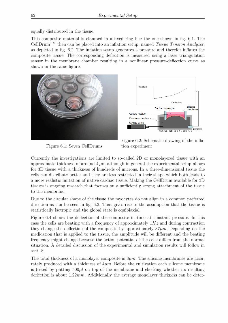
62 Experimental Setup
equally distributed in the tissue.
This composite material is clamped in a fixed ring like the one shown in fig. 6.1. TheCellDrumTM then can be placed into an inflation setup, named Tissue Tension Analyzer,as depicted in fig. 6.2. The inflation setup generates a pressure and therefor inflates thecomposite tissue. The corresponding deflection is measured using a laser triangulationsensor in the membrane chamber resulting in a nonlinear pressure-deflection curve asshown in the same figure.
Figure 6.1: Seven CellDrumsFigure 6.2: Schematic drawing of the infla-tion experiment
Currently the investigations are limited to so-called 2D or monolayered tissue with anapproximate thickness of around 4µm although in general the experimental setup allowsfor 3D tissue with a thickness of hundreds of microns. In a three-dimensional tissue thecells can distribute better and they are less restricted in their shape which both leads toa more realistic imitation of native cardiac tissue. Making the CellDrum available for 3Dtissues is ongoing research that focuses on a sufficiently strong attachment of the tissueto the membrane.
Due to the circular shape of the tissue the myocytes do not align in a common preferreddirection as can be seen in fig. 6.3. That gives rise to the assumption that the tissue isstatistically isotropic and the global state is equibiaxial.
Figure 6.4 shows the deflection of the composite in time at constant pressure. In thiscase the cells are beating with a frequency of approximately 1Hz and during contractionthey change the deflection of the composite by approximately 37µm. Depending on themedication that is applied to the tissue, the amplitude will be different and the beatingfrequency might change because the action potential of the cells differs from the normalsituation. A detailed discussion of the experimental and simulation results will follow insect. 8.
The total thickness of a monolayer composite is 8µm. The silicone membranes are accu-rately produced with a thickness of 4µm. Before the cultivation each silicone membraneis tested by putting 500µl on top of the membrane and checking whether its resultingdeflection is about 1.22mm. Additionally the average monolayer thickness can be deter-
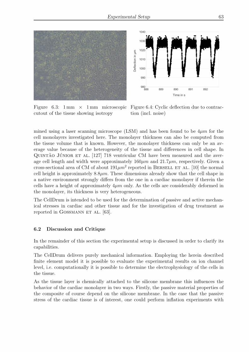
Experimental Setup 63
Figure 6.3: 1mm × 1mm microscopiccutout of the tissue showing isotropy
Figure 6.4: Cyclic deflection due to contrac-tion (incl. noise)
mined using a laser scanning microscope (LSM) and has been found to be 4µm for thecell monolayers investigated here. The monolayer thickness can also be computed fromthe tissue volume that is known. However, the monolayer thickness can only be an av-erage value because of the heterogeneity of the tissue and differences in cell shape. InQuintao Junior et al. [127] 718 ventricular CM have been measured and the aver-age cell length and width were approximately 160µm and 21.7µm, respectively. Given across-sectional area of CM of about 191µm2 reported in Bersell et al. [10] the normalcell height is approximately 8.8µm. These dimensions already show that the cell shape ina native environment strongly differs from the one in a cardiac monolayer if therein thecells have a height of approximately 4µm only. As the cells are considerably deformed inthe monolayer, its thickness is very heterogeneous.
The CellDrum is intended to be used for the determination of passive and active mechan-ical stresses in cardiac and other tissue and for the investigation of drug treatment asreported in Goßmann et al. [63].
6.2 Discussion and Critique
In the remainder of this section the experimental setup is discussed in order to clarify itscapabilities.
The CellDrum delivers purely mechanical information. Employing the herein describedfinite element model it is possible to evaluate the experimental results on ion channellevel, i.e. computationally it is possible to determine the electrophysiology of the cells inthe tissue.
As the tissue layer is chemically attached to the silicone membrane this influences thebehavior of the cardiac monolayer in two ways. Firstly, the passive material properties ofthe composite of course depend on the silicone membrane. In the case that the passivestress of the cardiac tissue is of interest, one could perform inflation experiments with
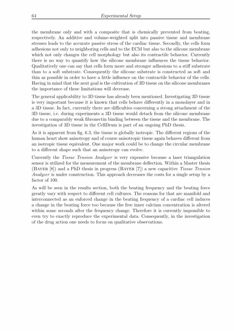
64 Experimental Setup
the membrane only and with a composite that is chemically prevented from beating,respectively. An additive and volume-weighted split into passive tissue and membranestresses leads to the accurate passive stress of the cardiac tissue. Secondly, the cells formadhesions not only to neighboring cells and to the ECM but also to the silicone membranewhich not only changes the cell morphology but also its contractile behavior. Currentlythere is no way to quantify how the silicone membrane influences the tissue behavior.Qualitatively one can say that cells form more and stronger adhesions to a stiff substratethan to a soft substrate. Consequently the silicone substrate is constructed as soft andthin as possible in order to have a little influence on the contractile behavior of the cells.Having in mind that the next goal is the cultivation of 3D tissue on the silicone membranesthe importance of these limitations will decrease.
The general applicability to 3D tissue has already been mentioned. Investigating 3D tissueis very important because it is known that cells behave differently in a monolayer and ina 3D tissue. In fact, currently there are difficulties concerning a strong attachment of the3D tissue, i.e. during experiments a 3D tissue would detach from the silicone membranedue to a comparably weak fibronectin binding between the tissue and the membrane. Theinvestigation of 3D tissue in the CellDrum is part of an ongoing PhD thesis.
As it is apparent from fig. 6.3, the tissue is globally isotropic. The different regions of thehuman heart show anisotropy and of course anisotropic tissue again behaves different froman isotropic tissue equivalent. One major work could be to change the circular membraneto a different shape such that an anisotropy can evolve.
Currently the Tissue Tension Analyzer is very expensive because a laser triangulationsensor is utilized for the measurement of the membrane deflection. Within a Master thesis(Bayer [8]) and a PhD thesis in progress (Bayer [7]) a new capacitive Tissue TensionAnalyzer is under construction. This approach decreases the costs for a single setup by afactor of 100.
As will be seen in the results section, both the beating frequency and the beating forcegreatly vary with respect to different cell cultures. The reasons for that are manifold andinterconnected as an enforced change in the beating frequency of a cardiac cell inducesa change in the beating force too because the free inner calcium concentration is alteredwithin some seconds after the frequency change. Therefore it is currently impossible toeven try to exactly reproduce the experimental data. Consequently, in the investigationof the drug action one needs to focus on qualitative observations.
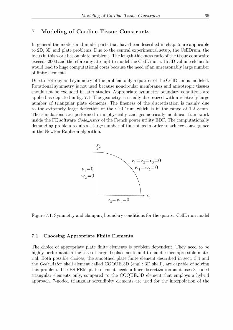
Modeling of Cardiac Tissue Constructs 65
7 Modeling of Cardiac Tissue Constructs
In general the models and model parts that have been described in chap. 5 are applicableto 2D, 3D and plate problems. Due to the central experimental setup, the CellDrum, thefocus in this work lies on plate problems. The length-thickness ratio of the tissue compositeexceeds 2000 and therefore any attempt to model the CellDrum with 3D volume elementswould lead to huge computational costs because the need of an unreasonably large numberof finite elements.
Due to isotropy and symmetry of the problem only a quarter of the CellDrum is modeled.Rotational symmetry is not used because noncircular membranes and anisotropic tissuesshould not be excluded in later studies. Appropriate symmetry boundary conditions areapplied as depicted in fig. 7.1. The geometry is usually discretized with a relatively largenumber of triangular plate elements. The fineness of the discretization is mainly dueto the extremely large deflection of the CellDrum which is in the range of 1.2–3mm.The simulations are performed in a physically and geometrically nonlinear frameworkinside the FE software Code Aster of the French power utility EDF. The computationallydemanding problem requires a large number of time steps in order to achieve convergencein the Newton-Raphson algorithm.
Figure 7.1: Symmetry and clamping boundary conditions for the quarter CellDrum model
7.1 Choosing Appropriate Finite Elements
The choice of appropriate plate finite elements is problem dependent. They need to behighly performant in the case of large displacements and to handle incompressible mate-rial. Both possible choices, the smoothed plate finite element described in sect. 3.4 andthe Code Aster shell element called COQUE 3D (engl.: 3D shell), are capable of solvingthis problem. The ES-FEM plate element needs a finer discretization as it uses 3-nodedtriangular elements only, compared to the COQUE 3D element that employs a hybridapproach. 7-noded triangular serendipity elements are used for the interpolation of the

66 Modeling of Cardiac Tissue Constructs
rotational degrees of freedom and 6-noded triangular Lagrange elements are used for thetranslational degrees of freedom. The performance of those two elements obviously is quitedifferent as they use interpolation functions of different degree and as the COQUE 3Delements employ a corotational framework. For the current problems, that are supposedto often show below 5% or at most 10% strain, both elements produce nearly equal results.The ES-FEM plate element is expected to perform better if the geometry becomes morecomplex and if the strains become larger because it is comparably insensitive to elementdistortion that is likely to occur in those cases.
7.2 Parameter Fitting
Currently we model the passive material response with the Neo-Hookean material. Itsstrain energy function Ψ in terms of the principal stretches λ = (λ1, λ2, λ3)
T reads as
Ψ(λ1, λ2, λ3) = C10(λ21 + λ2
2 + λ23 − 3) , (7.1)
with its material constant C10 that defines the slope of the nonlinear stress-strain curve.Taking into account the active component of the constitutive law one can specialize eq.(5.1) using eq. (5.61) to
S11 = 2C10 − p1
λ21
+ Tref(1 + β0(λ1 − 1))1
λ21
, (7.2)
at maximum activation z = 1. Of course eq. (5.61) of the HMT model can be replacedby the NHS version, eq. (5.66). The main mechanical parameters in this model are theNeo-Hookean material constant C10 and the tissue tension at rest Tref , both determinedby a parameter fitting. To this end we minimize
2C10 +1
λ21
(1 + β0(λ1 − 1))Tref − p1
λ21
− Se → Min , (7.3)
with respect to C10 and Tref with the stress Se obtained from the experiments. Theexperimental stress values can be determined by simple geometric considerations that areillustrated in fig. 7.2. It is obvious that for the circular isotropic membrane the stretch isequibiaxial and
λ1 = λ2 = λ =d2d1
(7.4)
holds with d1 being the initial diameter of the membrane and d2 the arc length in thedeflected state. λ3 = λ−2 can be obtained from the incompressibility condition J = 1 thathas been introduced in eqs. (7.2) and (7.3). The arc length can be computed from thecenter deflection u3 via
d2 =arctan
(2u3
d1
)
(4u23 + d21)
2u3. (7.5)
An expression for the experimentally determined 2nd Piola-Kirchhoff stress can been de-rived like for instance in Schomburg [136]. The balance of the pressure-induced vertical

Modeling of Cardiac Tissue Constructs 67
Figure 7.2: Illustration of the deflected CellDrum
force F P3 and the vertical component F F
3 of the force that is acting on the clamping frameas shown in fig. 7.2 reads as F P
3 = F F3 . Replacing F P
3 by the pressure acting on the circu-lar membrane and representing F F
3 by the membrane (experimental) stress Se acting onthe whole circumference of the frame and on the membrane thickness h, the balance ofvertical forces is given by
F P3 = Pπ
(d22
)2
= F F3 = Seh · 2π
d22
dw
dr
∣∣∣∣r=
d22
. (7.6)
The derivative of the deflection w in radial direction is included in order to get the verticalportion of F F . Given the approximation that the inflated membrane has a parabolic shape,its deflection w can be represented by
w(r) = u3
(
1−4r2
d22
)
. (7.7)
Carrying out the differentiation in eq. (7.6) leads to
Pπ
(d22
)2
= Seh · 2πd22u3
4
d2(7.8)
and reorganizing delivers the experimentally determined 2nd Piola-Kirchhoff stress
Se =P(d22
)2
4hu3. (7.9)
As usual in soft tissue biomechanics the poisson ratio ν is assumed to be close to 0.5.
With respect to the described parameter fitting the data for the membrane-tissue compos-ite yields C10 = 0.0838284 and Tref = 0.058kPa. A parameter fitting for measurements ofthe silicone membrane alone revealed C10 = 0.1840321. Thus, in the small strain regimethe membrane is approximately twice as stiff as the composite which proves that it in-fluences the contractility of the cardiac cells as discussed in sect. 6.2. This influence evengrows when large strains occur which is not the case for the results presented here, though.
68 Modeling of Cardiac Tissue Constructs
Another limitation of the parameter fitting is the assumption of a homogeneous andisotropic stretch although the local stretch of course depends on the tissue composition, alocal anisotropy and the activation state. In the fitting procedure these local differences aredisregarded and the average stretch λ is used instead. The assumption of global isotropyhas been verified in sect. 6.1.
Finally it should be mentioned that fig. 7.2 implies that the membrane inflates like afreely supported plate and is shaped like a sphere segment. From fig. 7.1 it is apparentthat the membrane is actually fully clamped and consequently the model in eq. (7.9) isonly an approximation.
7.3 Constitutive Tensor
In order to compute the stiffness matrices the constitutive tensor is needed. The stresscan be split up into three parts and so can the constitutive tensor
C = Cdev + Cvol + Ca . (7.10)
The deviatoric and volumetric parts of the constitutive tensor need not be derived here asthey represent the passive response of the material that is not in the focus of this thesis.Those derivations can be found in Holzapfel [72]. It is still necessary to derive Ca
Ca = 2∂Sa
∂C= 2
∂Sa
∂λ⊗
∂λ
∂C, (7.11)
the part of the constitutive tensor that arises from the cellular contraction. With
λ2 = a0 ·Ca0 = C · (a0 ⊗ a0) (7.12)
the derivative of the stretch with respect to the right Cauchy-Green tensor can be com-puted as follows
∂λ
∂C=
1
2(C · (a0 ⊗ a0))
−1
2
∂(C · (a0 ⊗ a0))
∂C
=1
2(a0 ·Ca0)
−1
2
∂(a0 ·Ca0)
∂C
=1
2λ−1∂C
∂C· (a0 ⊗ a0)
=1
2λ−1(a0 ⊗ a0) . (7.13)
In terms of the herein investigated circular membrane one can ideally assume that λ1 =λ2 = λ and λ3 = 1. Using the spectral decomposition of C,
C =
3∑
i=1
λ2iai ⊗ ai, (7.14)
Modeling of Cardiac Tissue Constructs 69
leads to
C = λ2(a1 ⊗ a1 + a2 ⊗ a2) = λ2R (7.15)
C−1 = λ−2RT = λ−2R. (7.16)
with R orthogonal and symmetric. The derivative of the active part of the 2nd Piola-Kirchhoff stress tensor with respect to the stretch then reads as
∂Sa
∂λ=
∂(T (t, λ)λ−2R)
∂λ
=
(∂T (t, λ)
∂λλ−2 − 2λ−3T (t, λ)
)
R
=(Trefβ0zλ
−2 − 2λ−3Tref(1 + β0(λ− 1))z)R
= Trefz(β0λ
−2 − 2λ−3 − 2λ−2β0 + 2λ−3β0
)R
= Trefzλ−2(2λ−1(β0 − 1)− β0)R . (7.17)
In the given isotropic application, R = I and one arrives at
Ca = 2∂Sa
∂λ⊗
∂λ
∂C(7.18)
= λ−3Trefz(2λ−1(β0 − 1)− β0)I ⊗ I . (7.19)
7.4 Model Summary
In order to facilitate the understanding of this multi-component model, fig. 7.3 depicts thebasic steps. Inflation experiments and drug testing are performed in the Lab of Medicaland Molecular Biology at Aachen University of Applied Sciences. These data can be usedto construct the model and to fit the mechanical model parameters.
The two systems of ordinary differential equations are solved at each time step at the levelof the constitutive equations. The models of cellular processes are parameterized solelyusing electrophysiological literature data. The nodal model provides the stimulus for theventricular model, thereby being the pacemaker.
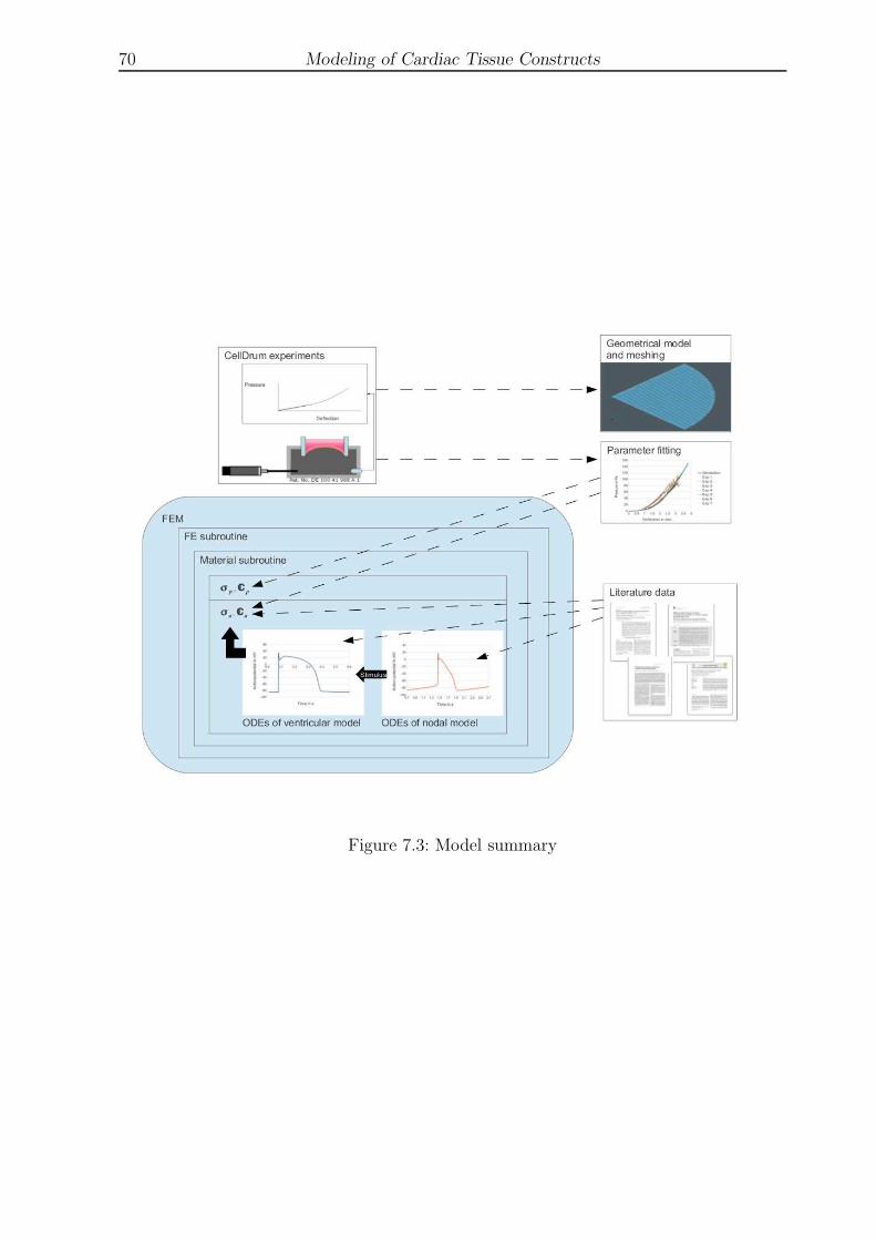
70 Modeling of Cardiac Tissue Constructs
Figure 7.3: Model summary
Implementation, Validation and Numerical Results 71
8 Implementation, Validation and Numerical Results
8.1 Implementations
8.1.1 Data Acquisition and Processing
The data acquisition from the CellDrum is implemented in LabView and further analyticsof the results is made through MS Excel or its non-commercial equivalent Libre OfficeCalc. The parameter fittings have been implemented in the software Scilab and statisticalanalysis of the pressure-deflection curves has been implemented in the statistics softwareR.
8.1.2 Finite Element Framework
As already indicated, the FE software in use is Code Aster which is developed by theFrench utility EDF. It is an open source software whose core is written in FORTRAN77until version 11.x. Most of the implementations have been done in Code Aster version10.6 and have been successfully tested in version 11.4 too. Starting from version 12.0 thecore of Code Aster is written in FORTRAN90 and the material subroutines written inthis thesis have been successfully converted to FORTRAN90 and tested in Code Asterversion 12.1. The administrative and configuration files as well as the user interfaces ofCode Aster are written in Python.
The pre- and post-processor that has been employed is called SALOME and also comesfrom EDF. Geometry creation and modification, meshing and graphical analysis of theresults can all be done in this software.
In order to prepare a simulation using Code Aster one needs to define a so-called commandfile. In this Python interpreted command file the mesh can be read in and modified, thematerial definitions are made, the boundary conditions are established, the solver can bechosen and configured and the results can be processed to prepare post-processing.
8.1.2.1 ES-FEM For the implementation of the plate smoothed FEM the so-called discrete Kirchhoff triangular (DKT) element of Code Aster has been modified. Theimplementation of the DKT element provides all the structures that are required in orderto be able to implement the plate ES-FE. The DKT element is a three-noded triangularplate element with three translational and three rotational degrees of freedom at eachnode. The only change to the element definition that has to be made is an increase of thebandwidth of the stiffness matrix because edge-based smoothing domains generally spanover two elements. The computation of the strain-displacement matrix and the stiffnessmatrix is made on element level by replacing the standard computation of the DKTelement.
Besides some work-around implementations to fit into the complex framework ofCode Aster the whole implementational work is limited to the element subroutine. It isongoing work to properly integrate the implementation into the Code Aster distributionmaking it available to the community.

72 Implementation, Validation and Numerical Results
8.1.2.2 Material Model The passive-active model for cardiac tissue is imple-mented on the level of the constitutive equation. The standard hyper-elastic materialmodel is used and the active part is additionally implemented. Within those subroutinesthe systems of ordinary differential equations are implemented that describe the cellularelectrophysiology of different cell types. Depending on the given problem the ventricularcell model can either be solved on each Gaussian point or only once. The nodal cell modelis always solved only once per time step as it has no influence to the beating force butonly serves as a pacemaker for the ventricular cells.
Some configuration files have been written in order to let the Code Aster distributionknow the material model.
The nonlinear equation systems are solved using a Newton-Raphson algorithm with arelative error of erel = 10−6 at discrete times ti. At each Gaussian point the stiff systemof ODEs is solved with an adaptive time stepping scheme in the way that the Newton-Raphson time interval [ti, ti+1] is further divided into m time steps because the electricalprocesses are much faster than the mechanical response. A fourth order singly-diagonalimplicit Runge-Kutta solver with adaptive time stepping (Hairer and Wanner [67])which has been shown to be unconditionally A-stable is used for the solution of the systemof ODEs.
8.2 Validation of S-FEM Implementation
Firstly the ES-FEM implementation for plate problems is validated for some aca-demic plane stress and plain strain problems that already have been presented inFrotscher and Staat [50]. They show the abilities of the ES-FEM in general andthe application to geometrically and materially nonlinear plates. Secondly the ES-FEMimplementation is applied to the CellDrum problem and performs well despite the extremeslenderness of the membrane.
8.2.1 Square Plate with Circular Hole
The first problem to be examined is a linear plane strain problem shown in fig. 8.1. Itillustrates a quarter of a square plate of size 10m× 10m with a circular hole of 1m radiusand the applied symmetry and traction boundary conditions. Its thickness is t = 1m. Thematerial has been chosen with E = 1000N/m2 and ν = 0.3. The problem domain hasbeen discretized with three-noded triangular elements as can be seen in fig. 8.2.
Figures 8.3 and 8.4 show the displacements u1 and u2 on the symmetry lines x2 = 0 andx1 = 0, respectively. The ES-FEM results achieved with linear triangular elements (ES-FEM-T3) are compared with the results achieved with standard FEM using triangularelements (FEM-T3, i.e. constant strain) and quadrilateral elements (FEM-Q4). The latterserves as the reference solution. It is obvious that the ES-FEM-T3 solution is nearly equalto the FEM-Q4 solution whereas FEM-T3 shows deficiencies. Especially with x1 → 1 andx2 → 1, i.e. next to the hole, the FEM-T3 solution differs significantly from the two othersolutions.
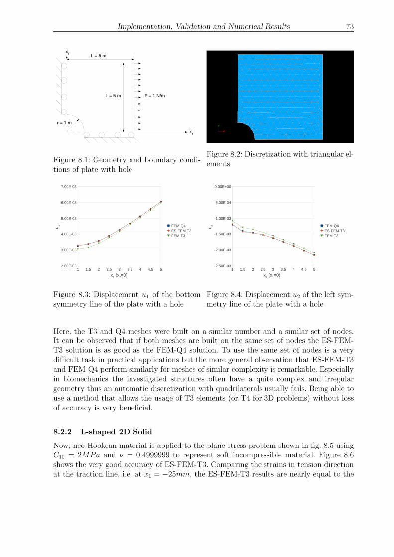
Implementation, Validation and Numerical Results 73
Figure 8.1: Geometry and boundary condi-tions of plate with hole
Figure 8.2: Discretization with triangular el-ements
Figure 8.3: Displacement u1 of the bottomsymmetry line of the plate with a hole
Figure 8.4: Displacement u2 of the left sym-metry line of the plate with a hole
Here, the T3 and Q4 meshes were built on a similar number and a similar set of nodes.It can be observed that if both meshes are built on the same set of nodes the ES-FEM-T3 solution is as good as the FEM-Q4 solution. To use the same set of nodes is a verydifficult task in practical applications but the more general observation that ES-FEM-T3and FEM-Q4 perform similarly for meshes of similar complexity is remarkable. Especiallyin biomechanics the investigated structures often have a quite complex and irregulargeometry thus an automatic discretization with quadrilaterals usually fails. Being able touse a method that allows the usage of T3 elements (or T4 for 3D problems) without lossof accuracy is very beneficial.
8.2.2 L-shaped 2D Solid
Now, neo-Hookean material is applied to the plane stress problem shown in fig. 8.5 usingC10 = 2MPa and ν = 0.4999999 to represent soft incompressible material. Figure 8.6shows the very good accuracy of ES-FEM-T3. Comparing the strains in tension directionat the traction line, i.e. at x1 = −25mm, the ES-FEM-T3 results are nearly equal to the
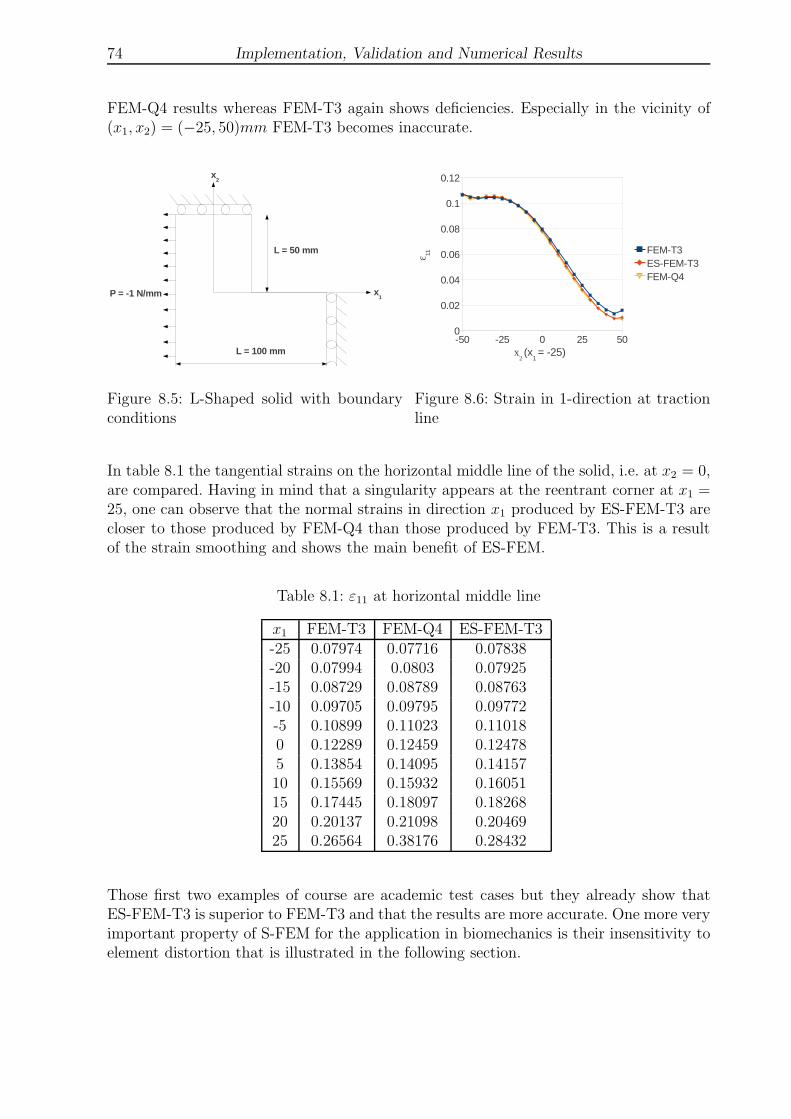
74 Implementation, Validation and Numerical Results
FEM-Q4 results whereas FEM-T3 again shows deficiencies. Especially in the vicinity of(x1, x2) = (−25, 50)mm FEM-T3 becomes inaccurate.
Figure 8.5: L-Shaped solid with boundaryconditions
Figure 8.6: Strain in 1-direction at tractionline
In table 8.1 the tangential strains on the horizontal middle line of the solid, i.e. at x2 = 0,are compared. Having in mind that a singularity appears at the reentrant corner at x1 =25, one can observe that the normal strains in direction x1 produced by ES-FEM-T3 arecloser to those produced by FEM-Q4 than those produced by FEM-T3. This is a resultof the strain smoothing and shows the main benefit of ES-FEM.
Table 8.1: ε11 at horizontal middle line
x1 FEM-T3 FEM-Q4 ES-FEM-T3-25 0.07974 0.07716 0.07838-20 0.07994 0.0803 0.07925-15 0.08729 0.08789 0.08763-10 0.09705 0.09795 0.09772-5 0.10899 0.11023 0.110180 0.12289 0.12459 0.124785 0.13854 0.14095 0.1415710 0.15569 0.15932 0.1605115 0.17445 0.18097 0.1826820 0.20137 0.21098 0.2046925 0.26564 0.38176 0.28432
Those first two examples of course are academic test cases but they already show thatES-FEM-T3 is superior to FEM-T3 and that the results are more accurate. One more veryimportant property of S-FEM for the application in biomechanics is their insensitivity toelement distortion that is illustrated in the following section.
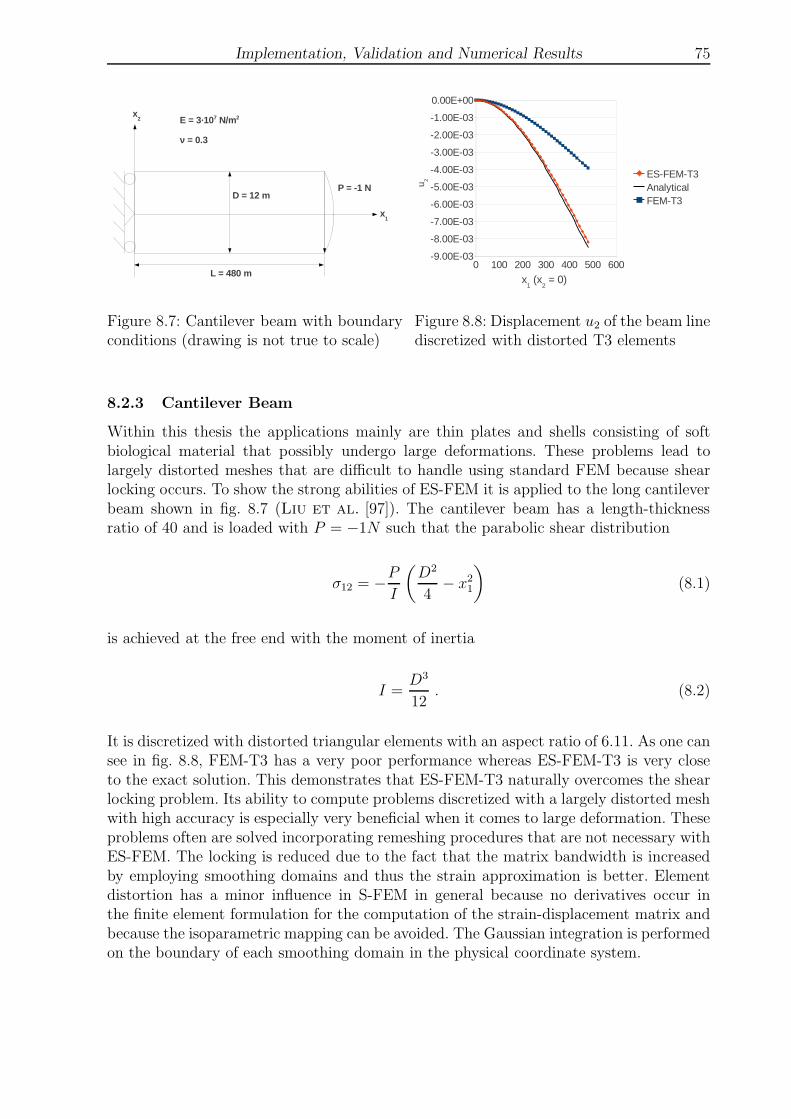
Implementation, Validation and Numerical Results 75
Figure 8.7: Cantilever beam with boundaryconditions (drawing is not true to scale)
Figure 8.8: Displacement u2 of the beam linediscretized with distorted T3 elements
8.2.3 Cantilever Beam
Within this thesis the applications mainly are thin plates and shells consisting of softbiological material that possibly undergo large deformations. These problems lead tolargely distorted meshes that are difficult to handle using standard FEM because shearlocking occurs. To show the strong abilities of ES-FEM it is applied to the long cantileverbeam shown in fig. 8.7 (Liu et al. [97]). The cantilever beam has a length-thicknessratio of 40 and is loaded with P = −1N such that the parabolic shear distribution
σ12 = −P
I
(D2
4− x2
1
)
(8.1)
is achieved at the free end with the moment of inertia
I =D3
12. (8.2)
It is discretized with distorted triangular elements with an aspect ratio of 6.11. As one cansee in fig. 8.8, FEM-T3 has a very poor performance whereas ES-FEM-T3 is very closeto the exact solution. This demonstrates that ES-FEM-T3 naturally overcomes the shearlocking problem. Its ability to compute problems discretized with a largely distorted meshwith high accuracy is especially very beneficial when it comes to large deformation. Theseproblems often are solved incorporating remeshing procedures that are not necessary withES-FEM. The locking is reduced due to the fact that the matrix bandwidth is increasedby employing smoothing domains and thus the strain approximation is better. Elementdistortion has a minor influence in S-FEM in general because no derivatives occur inthe finite element formulation for the computation of the strain-displacement matrix andbecause the isoparametric mapping can be avoided. The Gaussian integration is performedon the boundary of each smoothing domain in the physical coordinate system.

76 Implementation, Validation and Numerical Results
Figure 8.9: 4µm thick membrane seeded with 100µm thick tissue
8.3 Simulation of Cardiac Monolayers
The CellDrum setup described in sect. 6 up to now has been used for the investigationof cardiac monolayers that have a thickness of about 4µm. As the current plate ES-FEMimplementation does not incorporate a handling of large rotations, like for instance thecorotational approach, it converges very slowly when the deflection of the membrane be-comes very large. Thus for the current application we usually employ the Code Aster shellelement named COQUE 3D that has been mentioned in sect. 7.1 already. One drawback ofthose elements are stress oscillations close to regions where Dirichlet boundary conditionsare applied. Those oscillations do not appear for the ES-FEM-T3 elements.
As already indicated, both elements produce similar results and this is shown in fig. 8.9.For large rotations the ES-FEM-T3 element shows a much worse convergence behaviourconcerning the Newton iterations (although it always converges). ES-FEM-T3 is the el-ement of choice for so-called three-dimensional tissue layers with a thickness of about100µm. For 3D tissue layers the CellDrum problem is still a plate problem with a diame-ter to thickness ratio of 160.
Based on the implementations that have been done in this thesis, materially and geo-metrically nonlinear FS-FEM-T4 elements have been implemented in another PhD thesis(Duong [42]). As FS-FEM is the 3D equivalent of ES-FEM those tetrahedral elementshave very similar properties. Those elements can be employed when - apart from theinvestigation of the CellDrum experiments - 3D tissue simulations need to be performed.
Due to isotropy and symmetry the model only represents a quarter of the CellDrumand the applied appropriate boundary conditions are depicted in fig. 7.1. The fineness ofthe discretization mainly depends on the slenderness and the expected deflection of theCellDrum. It has a diameter of 16mm and in the case of a cell monolayer it has a thicknessof only 0.008mm. Therefore we have to deal with radius-thickness ratios of about 1000 anda maximum deflection of the membrane in the range of 2.5–3mm. This computationally
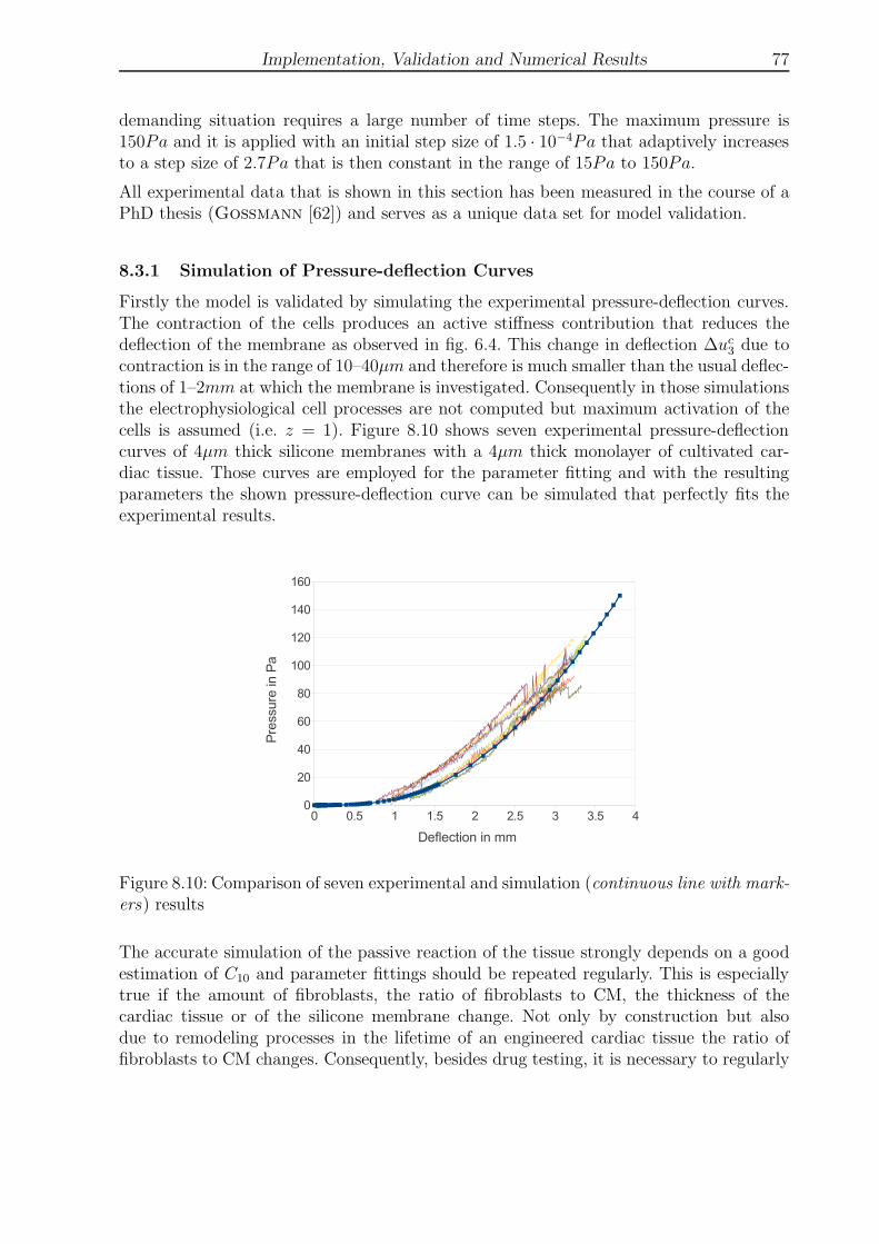
Implementation, Validation and Numerical Results 77
demanding situation requires a large number of time steps. The maximum pressure is150Pa and it is applied with an initial step size of 1.5 · 10−4Pa that adaptively increasesto a step size of 2.7Pa that is then constant in the range of 15Pa to 150Pa.
All experimental data that is shown in this section has been measured in the course of aPhD thesis (Goßmann [62]) and serves as a unique data set for model validation.
8.3.1 Simulation of Pressure-deflection Curves
Firstly the model is validated by simulating the experimental pressure-deflection curves.The contraction of the cells produces an active stiffness contribution that reduces thedeflection of the membrane as observed in fig. 6.4. This change in deflection ∆uc
3 due tocontraction is in the range of 10–40µm and therefore is much smaller than the usual deflec-tions of 1–2mm at which the membrane is investigated. Consequently in those simulationsthe electrophysiological cell processes are not computed but maximum activation of thecells is assumed (i.e. z = 1). Figure 8.10 shows seven experimental pressure-deflectioncurves of 4µm thick silicone membranes with a 4µm thick monolayer of cultivated car-diac tissue. Those curves are employed for the parameter fitting and with the resultingparameters the shown pressure-deflection curve can be simulated that perfectly fits theexperimental results.
Figure 8.10: Comparison of seven experimental and simulation (continuous line with mark-ers) results
The accurate simulation of the passive reaction of the tissue strongly depends on a goodestimation of C10 and parameter fittings should be repeated regularly. This is especiallytrue if the amount of fibroblasts, the ratio of fibroblasts to CM, the thickness of thecardiac tissue or of the silicone membrane change. Not only by construction but alsodue to remodeling processes in the lifetime of an engineered cardiac tissue the ratio offibroblasts to CM changes. Consequently, besides drug testing, it is necessary to regularly
78 Implementation, Validation and Numerical Results
repeat the plain inflation experiments in order to be able to properly parameterize themodels. On the other hand the computational model can be improved by incorporatingthe amount of fibroblasts directly as discussed in sect. 9.2.5.
8.3.2 Simulation of Cell Contraction
To simulate single or multiple contractions one can start the contraction process at a cer-tain point of the simulation result in fig. 8.10. This starting point can be chosen dependingon the experimental results as follows.
From the experiments one is able to extract the deflection of the membrane when the cellsare inactivated. For clarity fig. 8.11 shows an experimental result that has a deflectionat rest of 1.23mm and compares it to a simulation result. Even with an equal pressure adifferent membrane will have a different deflection at rest in the order of approximately0.05mm because it is not possible to accurately reproduce the biological tissues. To providea good accuracy of the simulations one can select a time step of the pressure-deflectionsimulation in sect. 8.3.1 at which the membrane has a deflection that is close to the oneshown in the experiments. If that does not provide sufficient accuracy one can simulateup to a pressure such that the proper deflection at rest is achieved in the simulation. Itcan be seen in fig. 8.10 that it is generally possible to simulate any membrane deflectionin the experimental range.
Starting from this resting state when the cells are inactive. One can now simulate one ormultiple contractions using all parts of the model, i.e. computing the electrophysiologicalprocesses on cell level and use the resulting free inner calcium concentration as an inputto the mechanical part of the constitutive model at time ti. The time steps ∆ti = ti+1− tineed to be chosen in the way so that the mechanical response of the model is sufficientlyaccurate. The electrophysiological processes are much faster and therefore are computedin adaptively subdivided time steps.
Figure 8.11 compares one contraction of the CellDrum with two simulation results. Itis obvious that the change in deflection is nearly the same in all the cases. Thus thecontractility of the cells can be captured very well by the model.
One also observes that the duration of the deflection, i.e. the contraction time is muchshorter in the simulation where the MNT Purkinje fiber model has been used in conjunc-tion with the HMT model (0.2s vs. 0.6s). This effect leads to the assumption that themechanical response of the applied model is too fast. Possible reasons have been identifiedthat explain the discrepancy:
Depending on the specific cell type the speed of development of free intra-cellularcalcium concentration is different. As the literature data provides a wide range ofresults the parameter set of the system of ODEs might have to be adjusted accordingto the respective cell type. Currently there are a lot of uncertainties concerning theactual cell types that are represented in the monolayer, their degree of maturity, thecell environment and literature data is often very specific and does not fully fit.
The time rate of muscle activation z (cf. eq. (5.67)) depends on the free intra-

Implementation, Validation and Numerical Results 79
cellular calcium concentration. Again, it might be the rate constants that need tobe adjusted to the cell type.
It has been mentioned in Ruiz-Baier et al. [132] that today’s models directlyuse cellular models on tissue level without properly scaling or averaging the cellularcontributions to the passive or active stress in the tissue with respect to cell volumeportion or cell distribution. Necessarily, the mechanical reaction of the tissue on theelectrophysiological processes is much more direct than it would be with a so-calledhomogenization that is discussed in sect. 9.2.7.
The current model assumes that all the cells in the monolayer contract syn-chronously. In reality the action potential is transmitted through the monolayervia gap junctions that connect neighboring cells to each other. This again wouldlead to a slower mechanical response.
Figure 8.11: Comparison of MNT-HMT(blue continuous line with square markers)and TT-NHS (yellow continuous line withtriangular markers) simulations with exper-imental results (red dashed line) with re-spect to ∆uc
3
Figure 8.12: Comparison of simulationspaced with a current density of 52pA · pF−1
at 1Hz (blue continuous line with squaremarkers) and 0.7Hz (red continuous linewith diamond markers) with respect to ∆uc
3
The second simulation curve has been computed using the TT human ventricular modelin conjunction with the NHS excitation-contraction coupling. It can clearly be seen thatthe duration of the contraction, i.e. the shape of the curve agrees much better with theexperimental findings. This is more due to the changes made in the NHS model withrespect to the HMT model as explained in sect. 5.4.4.2 rather than due to the differentelectrophysiological model that is employed. Especially the splitting of the tropomyosinrelaxation into slow and fast terms is supposed to drive those differences.
It has to be mentioned that there even seems to be a quantitative agreement between thecurves in fig. 8.11. The question that arises is whether this is generally true and it can only

80 Implementation, Validation and Numerical Results
be answered partially by this thesis as the amount of available experimental data is quitelow. However, the following results indicate that a quantitative agreement is achieved. Inthe following section some experimental results are shown for drug action on the CellDrumtissue and in the experimental results one recognizes strong differences in the beatingfrequencies of the control groups. It has already been mentioned that a so-called staircaseeffect exists that stands for positive relation between beating frequency and contractileforce, i.e. if the beating frequency increases, the contractile force increases too and viceversa. In fig. 8.12 the TT model has been paced externally at two different frequencies andafter a 60s pre-equilibration phase the contractile force is considerably different betweenthe two simulations. The pre-equilibration phase is necessary because the model needssome time to adjust to the new beating frequency just like real cells. Accounting for thestaircase effect indeed gives a fairly good quantitative agreement between the experimentaland simulated change in deflection as can be seen from table 8.2.
Table 8.2: Comparison of experimental (m = 3) and simulated maximum change in de-flection at different beating frequencies in mm
f = 0.5Hz f = 1.0HzExperiment 0.00913 0.02735Simulation 0.00462 0.02764
Nevertheless, respecting the given data, it currently is not possible to reliably compareeffects quantitatively. Therefore the following results are partially normalized to facilitatethe interpretation of the results. However, the results are not normalized in some diagramsif quantitative differences are important to be shown.
8.3.3 Drug Action
This section shows simulation results for the drugs named in sect. 4.4 and discusses themby comparison to CellDrum results and to findings from literature. Most of the resultshave already been published in Frotscher et al. [53; 54].
The results need to be regarded with respect to the fact that, although a lot of electro-physiological experiments have been performed all over the world for measuring the actionpotential of single cells, the action potential conduction through cell clusters, individualcurrents as well as intra- and extracellular ion concentrations, the gathered informationvaries. The experimental data strongly depend on the cell type, their maturity, the pro-duction batch, the investigated species, the experimental setup, the environment of thecells and many more. Therefore the data differ in the reported beating force, cell stresses,beating frequency, action potential shifts and IC50 values. The data are selected suchthat it fits the CellDrum experimental setup the most but often even this very care-fully selected information varies quite much. In some cases reliable data could not befound for human induced pluripotent stem cells. Thus data from different cells need tobe taken. Even under relatively well-controlled and well-known conditions the mechanicalCellDrum results themselves vary for the named reasons. Currently there are only few se-tups that measure mechanical parameters like the CellDrum, e.g. Grosberg et al. [64],

Implementation, Validation and Numerical Results 81
Nawroth et al. [111], Agarwal et al. [2] and Pakazad et al. [125] but so farthey have not been regarded for comparison because of the aforementioned uncertain-ties.
In the following all the results are collected comparing experimental and simulation re-sults of drug action on cardiac monolayers. If not stated otherwise, the inotropic andchronotropic drug effects have been simulated with the TT-NHS model and the Stewartmodel, respectively. For each respective drug the employed data for modeling the drugaction, as described in sect. 5.4.2, are summarized in a table including the source whereit has been obtained from.
8.3.3.1 Lidocaine Figures 8.13 and 8.14 show the simulated influence of Lido-caine to the change in deflection of the membrane and to the beating frequency of thecells at different concentrations and corresponding experimental results obtained fromCellDrum experiments. According to table 8.3 an IC50 value of 50µM is applied to both,the activation gate of the fast sodium channel and the activation gate of the pacemakercurrent.
Table 8.3: IC50 values for Lidocaine
IC50 Ion channel Species and cell type Reference11.2µM Nav1.5 HiPSc-derived cardiomyocytes Sirenko et al. [140]70µM Nav1.5 HiPSc-derived cardiomyocytes Terasawa [148]20µM Sodium Mouse eSc-derived cardiomyocytes Stoelzle et al. [144]61µM Sodium Freshly isolated rat cardiac myocytes Hill et al. [70]20–70µM HCN Xenopus laevis Oocytes Meng et al. [105]
Figure 8.13: Lidocaine affecting contractibil-ity in experiment (dashed) and simulation(continuous); sample size m = 3
Figure 8.14: Lidocaine affecting beating fre-quency in experiment (dashed) and simula-tion (continuous); sample size m = 3
Clearly both, the simulated dose-dependent change in beating force and in heart rate, arein good agreement with the experimental results. Within the range of 0–100µM of appliedLidocaine, the beating force seems to be linearly dose-dependent. The model even captures
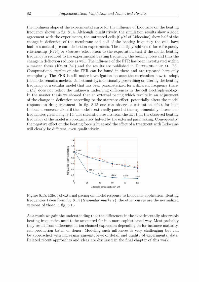
82 Implementation, Validation and Numerical Results
the nonlinear slope of the experimental curve for the influence of Lidocaine on the beatingfrequency shown in fig. 8.14. Although, qualitatively, the simulation results show a goodagreement with the experiments, the untreated cells (0µM of Lidocaine) show half of thechange in deflection of the membrane and half of the beating frequency the cells havehad in standard pressure-deflection experiments. The multiply addressed force-frequencyrelationship (FFR) or staircase effect leads to the expectation that if the model beatingfrequency is reduced to the experimental beating frequency, the beating force and thus thechange in deflection reduces as well. The influence of the FFR has been investigated withina master thesis (Koch [84]) and the results are published in Frotscher et al. [56].Computational results on the FFR can be found in there and are repeated here onlyexemplarily. The FFR is still under investigation because the mechanism how to adoptthe model remains unclear. Unfortunately, intentionally prescribing or altering the beatingfrequency of a cellular model that has been parameterized for a different frequency (here:1Hz) does not reflect the unknown underlying differences in the cell electrophysiology.In the master thesis we showed that an external pacing which results in an adjustmentof the change in deflection according to the staircase effect, potentially alters the modelresponse to drug treatment. In fig. 8.15 one can observe a saturation effect for highLidocaine concentrations if the model is externally paced at the experimentally determinedfrequencies given in fig. 8.14. The saturation results from the fact that the observed beatingfrequency of the model is approximately halved by the external pacemaking. Consequently,the negative effect on the beating force is huge and the effect of a treatment with Lidocainewill clearly be different, even qualitatively.
Figure 8.15: Effect of external pacing on model response to Lidocaine application. Beatingfrequencies taken from fig. 8.14 (triangular markers); the other curves are the normalizedversions of those in fig. 8.13
As a result we gain the understanding that the differences in the experimentally observablebeating frequencies need to be accounted for in a more sophisticated way. Most probablythey result from differences in ion channel expression depending on for instance maturity,cell production batch or donor. Modeling such influences is very challenging but canbe approached with increasing amount, level of detail and quality of experimental data.Related recent approaches and ideas are discussed in the final chapter of this work.
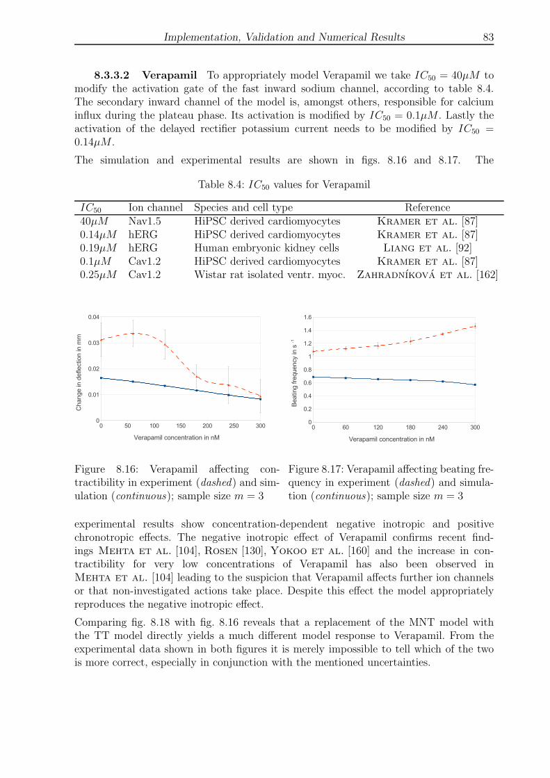
Implementation, Validation and Numerical Results 83
8.3.3.2 Verapamil To appropriately model Verapamil we take IC50 = 40µM tomodify the activation gate of the fast inward sodium channel, according to table 8.4.The secondary inward channel of the model is, amongst others, responsible for calciuminflux during the plateau phase. Its activation is modified by IC50 = 0.1µM . Lastly theactivation of the delayed rectifier potassium current needs to be modified by IC50 =0.14µM .
The simulation and experimental results are shown in figs. 8.16 and 8.17. The
Table 8.4: IC50 values for Verapamil
IC50 Ion channel Species and cell type Reference40µM Nav1.5 HiPSC derived cardiomyocytes Kramer et al. [87]0.14µM hERG HiPSC derived cardiomyocytes Kramer et al. [87]0.19µM hERG Human embryonic kidney cells Liang et al. [92]0.1µM Cav1.2 HiPSC derived cardiomyocytes Kramer et al. [87]0.25µM Cav1.2 Wistar rat isolated ventr. myoc. Zahradnıkova et al. [162]
Figure 8.16: Verapamil affecting con-tractibility in experiment (dashed) and sim-ulation (continuous); sample size m = 3
Figure 8.17: Verapamil affecting beating fre-quency in experiment (dashed) and simula-tion (continuous); sample size m = 3
experimental results show concentration-dependent negative inotropic and positivechronotropic effects. The negative inotropic effect of Verapamil confirms recent find-ings Mehta et al. [104], Rosen [130], Yokoo et al. [160] and the increase in con-tractibility for very low concentrations of Verapamil has also been observed inMehta et al. [104] leading to the suspicion that Verapamil affects further ion channelsor that non-investigated actions take place. Despite this effect the model appropriatelyreproduces the negative inotropic effect.
Comparing fig. 8.18 with fig. 8.16 reveals that a replacement of the MNT model withthe TT model directly yields a much different model response to Verapamil. From theexperimental data shown in both figures it is merely impossible to tell which of the twois more correct, especially in conjunction with the mentioned uncertainties.
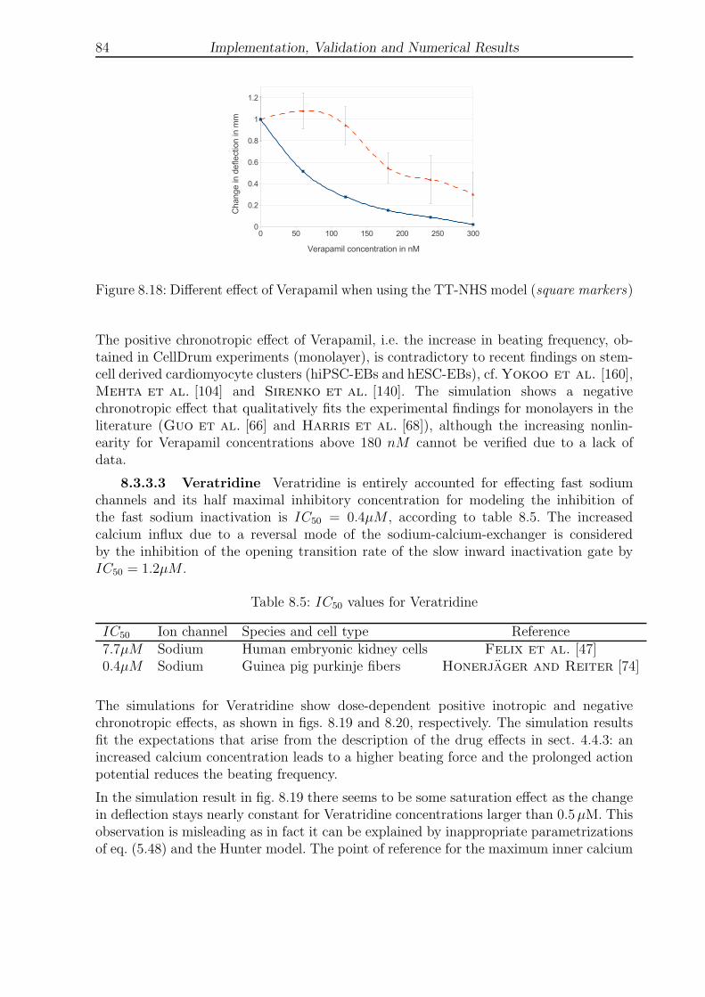
84 Implementation, Validation and Numerical Results
Figure 8.18: Different effect of Verapamil when using the TT-NHS model (square markers)
The positive chronotropic effect of Verapamil, i.e. the increase in beating frequency, ob-tained in CellDrum experiments (monolayer), is contradictory to recent findings on stem-cell derived cardiomyocyte clusters (hiPSC-EBs and hESC-EBs), cf.Yokoo et al. [160],Mehta et al. [104] and Sirenko et al. [140]. The simulation shows a negativechronotropic effect that qualitatively fits the experimental findings for monolayers in theliterature (Guo et al. [66] and Harris et al. [68]), although the increasing nonlin-earity for Verapamil concentrations above 180 nM cannot be verified due to a lack ofdata.
8.3.3.3 Veratridine Veratridine is entirely accounted for effecting fast sodiumchannels and its half maximal inhibitory concentration for modeling the inhibition ofthe fast sodium inactivation is IC50 = 0.4µM , according to table 8.5. The increasedcalcium influx due to a reversal mode of the sodium-calcium-exchanger is consideredby the inhibition of the opening transition rate of the slow inward inactivation gate byIC50 = 1.2µM .
Table 8.5: IC50 values for Veratridine
IC50 Ion channel Species and cell type Reference7.7µM Sodium Human embryonic kidney cells Felix et al. [47]0.4µM Sodium Guinea pig purkinje fibers Honerjager and Reiter [74]
The simulations for Veratridine show dose-dependent positive inotropic and negativechronotropic effects, as shown in figs. 8.19 and 8.20, respectively. The simulation resultsfit the expectations that arise from the description of the drug effects in sect. 4.4.3: anincreased calcium concentration leads to a higher beating force and the prolonged actionpotential reduces the beating frequency.
In the simulation result in fig. 8.19 there seems to be some saturation effect as the changein deflection stays nearly constant for Veratridine concentrations larger than 0.5µM. Thisobservation is misleading as in fact it can be explained by inappropriate parametrizationsof eq. (5.48) and the Hunter model. The point of reference for the maximum inner calcium
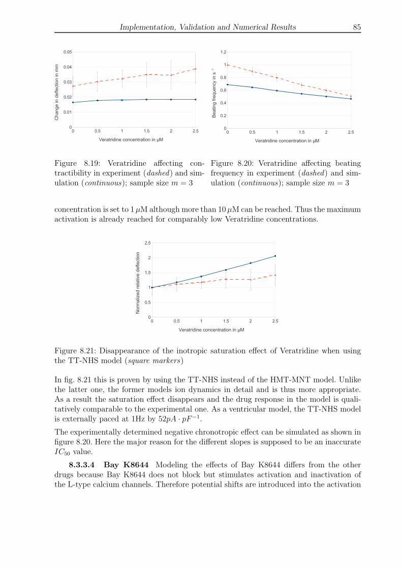
Implementation, Validation and Numerical Results 85
Figure 8.19: Veratridine affecting con-tractibility in experiment (dashed) and sim-ulation (continuous); sample size m = 3
Figure 8.20: Veratridine affecting beatingfrequency in experiment (dashed) and sim-ulation (continuous); sample size m = 3
concentration is set to 1µM although more than 10µM can be reached. Thus the maximumactivation is already reached for comparably low Veratridine concentrations.
Figure 8.21: Disappearance of the inotropic saturation effect of Veratridine when usingthe TT-NHS model (square markers)
In fig. 8.21 this is proven by using the TT-NHS instead of the HMT-MNT model. Unlikethe latter one, the former models ion dynamics in detail and is thus more appropriate.As a result the saturation effect disappears and the drug response in the model is quali-tatively comparable to the experimental one. As a ventricular model, the TT-NHS modelis externally paced at 1Hz by 52pA · pF−1.
The experimentally determined negative chronotropic effect can be simulated as shown infigure 8.20. Here the major reason for the different slopes is supposed to be an inaccurateIC50 value.
8.3.3.4 Bay K8644 Modeling the effects of Bay K8644 differs from the otherdrugs because Bay K8644 does not block but stimulates activation and inactivation ofthe L-type calcium channels. Therefore potential shifts are introduced into the activation
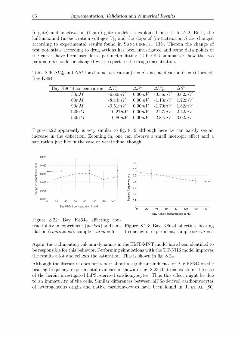
86 Implementation, Validation and Numerical Results
(d-gate) and inactivation (f-gate) gate models as explained in sect. 5.4.2.2. Both, thehalf-maximal (in-)activation voltages V50 and the slope of (in-)activation S are changedaccording to experimental results found in Sanguinetti [135]. Therein the change oftest potentials according to drug actions has been investigated and some data points ofthe curves have been used for a parameter fitting. Table 8.6 summarizes how the twoparameters should be changed with respect to the drug concentration.
Table 8.6: ∆V x50 and ∆Sx for channel activation (x = a) and inactivation (x = i) through
Bay K8644
Bay K8644 concentration ∆V a50 ∆Sa ∆V i
50 ∆Si
30nM -6.60mV 0.00mV -0.56mV 0.62mV60nM -8.44mV 0.00mV -1.13mV 1.22mV90nM -9.51mV 0.00mV -1.70mV 1.82mV120nM -10.27mV 0.00mV -2.27mV 2.42mV150nM -10.86mV 0.00mV -2.84mV 3.02mV
Figure 8.22 apparently is very similar to fig. 8.19 although here we can hardly see anincrease in the deflection. Zooming in, one can observe a small inotropic effect and asaturation just like in the case of Veratridine, though.
Figure 8.22: Bay K8644 affecting con-tractibility in experiment (dashed) and sim-ulation (continuous); sample size m = 5
Figure 8.23: Bay K8644 affecting beatingfrequency in experiment; sample size m = 5
Again, the rudimentary calcium dynamics in the HMT-MNT model have been identified tobe responsible for this behavior. Performing simulations with the TT-NHS model improvesthe results a lot and relaxes the saturation. This is shown in fig. 8.24.
Although the literature does not report about a significant influence of Bay K8644 on thebeating frequency, experimental evidence is shown in fig. 8.23 that one exists in the caseof the herein investigated hiPSc-derived cardiomyocytes. Thus this effect might be dueto an immaturity of the cells. Similar differences between hiPSc-derived cardiomyocytesof heterogeneous origin and native cardiomyocytes have been found in Ji et al. [80]
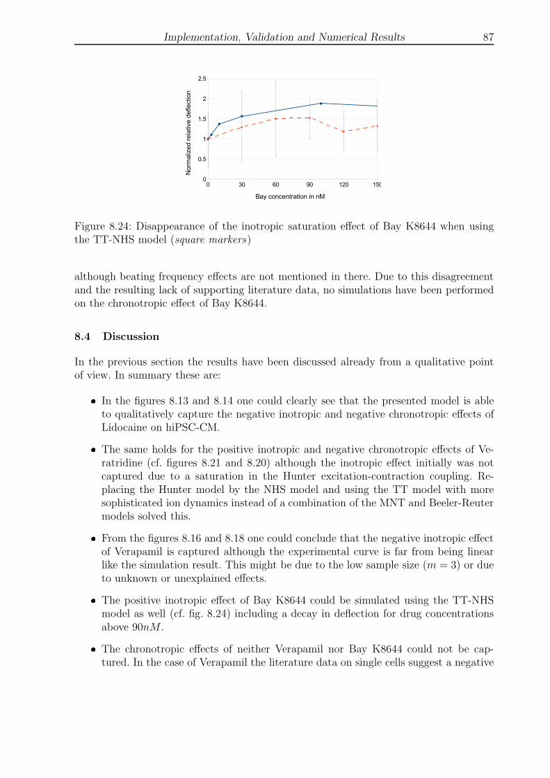
Implementation, Validation and Numerical Results 87
Figure 8.24: Disappearance of the inotropic saturation effect of Bay K8644 when usingthe TT-NHS model (square markers)
although beating frequency effects are not mentioned in there. Due to this disagreementand the resulting lack of supporting literature data, no simulations have been performedon the chronotropic effect of Bay K8644.
8.4 Discussion
In the previous section the results have been discussed already from a qualitative pointof view. In summary these are:
In the figures 8.13 and 8.14 one could clearly see that the presented model is ableto qualitatively capture the negative inotropic and negative chronotropic effects ofLidocaine on hiPSC-CM.
The same holds for the positive inotropic and negative chronotropic effects of Ve-ratridine (cf. figures 8.21 and 8.20) although the inotropic effect initially was notcaptured due to a saturation in the Hunter excitation-contraction coupling. Re-placing the Hunter model by the NHS model and using the TT model with moresophisticated ion dynamics instead of a combination of the MNT and Beeler-Reutermodels solved this.
From the figures 8.16 and 8.18 one could conclude that the negative inotropic effectof Verapamil is captured although the experimental curve is far from being linearlike the simulation result. This might be due to the low sample size (m = 3) or dueto unknown or unexplained effects.
The positive inotropic effect of Bay K8644 could be simulated using the TT-NHSmodel as well (cf. fig. 8.24) including a decay in deflection for drug concentrationsabove 90nM .
The chronotropic effects of neither Verapamil nor Bay K8644 could not be cap-tured. In the case of Verapamil the literature data on single cells suggest a negative
88 Implementation, Validation and Numerical Results
chronotropic effect whereas in monolayers the effect is positive. Of course the singlecell MNT and TT models are not able to capture this effect without major modifi-cation (cf. fig 8.17). In the case of Bay K8644 no chronotropic effects are reportedin the literature at all whereas a negative chronotropic effect could be observed inthe CellDrum experiments (cf. 8.23).
Including the FFR into the model is promising (see also Frotscher et al. [56])but with an external pacing there is an overreaction of the model. An alternativewill be discussed in sec. 9.2.2.
From a quantitative point of view one can state that in the control groups, i.e. withoutdrug treatment, neither the simulated contractile change in deflection nor the beatingfrequency are equal to the experimental values. The reasons are quite manifold but thetwo major reasons are the FFR and the immaturity of the hiPSC-CM. Respecting the FFRin an appropriate way, i.e. by reparameterization of the model according to experimentallyobserved beating frequencies will adjust the beating force and thus the contractile changein deflection as well. First investigations in Frotscher et al. [56] show that the FFRindeed has a strong effect and should be regarded in modeling.
The immaturity of the hiPSC-CM though is a generic term for the lack of knowledge on thephenotypical expression of the individual ion channels in hiPSC-CM compared to nativemammalian and human CM. The in vitro differentiation processes do not entirely reflectthe in vivo processes and therefore some channels might express differently. Moreover thematurity of the cells depends on how long after the day of cultivation the experiments areperformed. For this influence to be included in the model many patch clamp and MEAexperiments are required. This way one could clearly specify the differences between theinvestigated hiPSC-CM and native CM and derive better predictions of drug effects.Computational models could support this by parameter studies that help to find the ionchannels in question.
8.5 Simulation of Cardiac 3D Tissue
The heart of course is a 3D structure and it is well known that cells behave differentlydepending on their environment. This is especially true for a cell monolayer in whichthe cells are not organized in a 3D tissue. In a monolayer they can only communicatewith each other in a 2D plane. Moreover the mechanical environment is influenced by thesurface of the silicone membrane and the cells are flat in a monolayer whereas their shapeis significantly different in a 3D tissue. Nevertheless, investigating cell monolayers firstis a reasonable approach as this simplification leads to much more basic results. Duringthis thesis no 3D tissues (t > 100µm) have been investigated on the CellDrum which ismainly due to manufacturing problems. The chemical fixation of the tissue containing thehiPSc-derived cardiac myocytes at this time was not strong enough to reliably connect a3D tissue to the silicone membrane. Thus, lacking experimental data for 3D tissue it wasnecessary to focus on simulations of 2D tissue and the respective drug action.
First attempts to create 3D tissue consisting of hiPSC-CM and to investigate it in an
Implementation, Validation and Numerical Results 89
experimental setup have been successful as for instance inMathur et al. [102]. Thereinthe authors built a microfluidic device to measure the beating rate of the tissue based oncomputational motion-tracking in control conditions and with the option to apply drugs.
Surely the model can be applied to 3D tissues in the CellDrum setup as well althoughsome changes will have to be made then:
First of all the problem formulation will be three-dimensional and replace the plateformulation. This requires the usage of different finite elements. Regarding the re-sults obtained by Duong [42], a face-based smoothed finite element might be agood choice.
The implemented material models and especially the electrophysiological modelsare implemented for a 2D domain. Those models need to be extended to the thirddimension.
In a larger piece of tissue than the one investigated here, the propagation of themembrane potential through the tissue has a large effect on the mechanical behavior.Moreover the heart only works if the electrical propagation works appropriately.Thus this needs to be modeled appropriately and also in three dimensions.

Summary and Conclusion 91
9 Summary and Conclusion
The central goal of this work was the computational investigation of drug action oncardiac tissue. Regarding the complexity of the human heart on each length scale, asimplifying inflation test, called CellDrum, has been chosen to measure beating forcesand frequencies of cardiac monolayers. The system provides mechanical data for a cardiacmonolayer consisting of hiPSC-derived cardiomyocytes, fibroblasts and an ECM that ischemically fixed on an ultra-thin silicone membrane.
The mechanical experimental data has been used as input and validation data for a FEbased computational model. The shell FE model is able to capture the mechanics ofthe system and appropriate cellular electrophysiology models including the excitation-contraction coupling have been introduced on the level of the constitutive equations.
In the previous chapter the reader could see the capabilities of the model and the pur-pose of the following sections is mainly to point out necessary and nice-to-have modelimprovements and to point into rewarding future directions of research, especially con-cerning patient-specific investigation of drug action.
9.1 ES-FEM in Soft Tissue Mechanics
The edge-based S-FEM has been applied to the presented biomechanical plate problem.This method smooths a compatible, element-wise constant strain field across the edges ofa standard FE mesh. Converting the integrals over smoothing domains to boundary in-tegrals, the derivatives of shape functions and the isoparametric concept can be avoided.It has been shown that the ES-FEM-T3 element is superior to the standard FEM-T3element and can be as accurate as the standard FEM-Q4. The only drawback is an in-crease in matrix bandwidth that is more than compensated by the gain in accuracy andthe following properties of the method. For both, plate and three-dimensional applica-tions (FS-FEM), it is a method that facilitates the handling of volumetric locking, meshdistortion, shear locking and that avoids remeshing.
Today, geometrical models of anatomical structures are very often created fromMRI data, plastinates or other image processing methods, for instance for theheart (Jiang et al. [81]) and for pelvic floor structures (Bhattarai et al. [12] andvan der Giessen et al. [153]). Especially in these non-generic models, automaticmeshing algorithms often produce highly distorted elements from the image processingdata. ES-FEM and FS-FEM do not only improve the accuracy of T3 and T4 elements,respectively, which might lead to the preference of T3 and T4 elements over T6 and T8elements in some applications. Maybe even more importantly they avoid a singularity ofthe system matrix for very large aspect ratios. To demonstrate this the cantilever beamshown in figure 8.7 has been stretched to a length of 4800m and the tip load has beenmodified by P = 0.001N . The elements show aspect ratios greater than 50 and table9.1 shows that standard FEM can hardly produce a solution different from zero and forslightly larger aspect ratios it will give a singular system matrix. ES-FEM on the otherhand keeps two more decimal places and thus is able to handle much higher aspect ra-
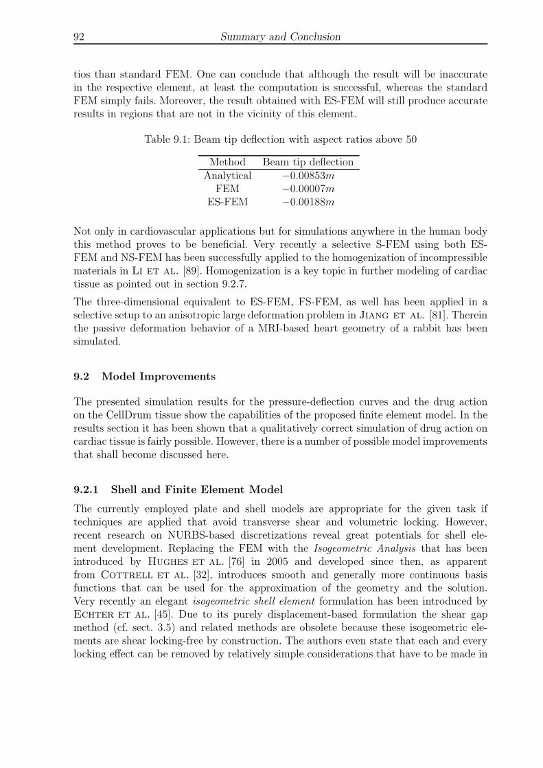
92 Summary and Conclusion
tios than standard FEM. One can conclude that although the result will be inaccuratein the respective element, at least the computation is successful, whereas the standardFEM simply fails. Moreover, the result obtained with ES-FEM will still produce accurateresults in regions that are not in the vicinity of this element.
Table 9.1: Beam tip deflection with aspect ratios above 50
Method Beam tip deflectionAnalytical −0.00853m
FEM −0.00007mES-FEM −0.00188m
Not only in cardiovascular applications but for simulations anywhere in the human bodythis method proves to be beneficial. Very recently a selective S-FEM using both ES-FEM and NS-FEM has been successfully applied to the homogenization of incompressiblematerials in Li et al. [89]. Homogenization is a key topic in further modeling of cardiactissue as pointed out in section 9.2.7.
The three-dimensional equivalent to ES-FEM, FS-FEM, as well has been applied in aselective setup to an anisotropic large deformation problem in Jiang et al. [81]. Thereinthe passive deformation behavior of a MRI-based heart geometry of a rabbit has beensimulated.
9.2 Model Improvements
The presented simulation results for the pressure-deflection curves and the drug actionon the CellDrum tissue show the capabilities of the proposed finite element model. In theresults section it has been shown that a qualitatively correct simulation of drug action oncardiac tissue is fairly possible. However, there is a number of possible model improvementsthat shall become discussed here.
9.2.1 Shell and Finite Element Model
The currently employed plate and shell models are appropriate for the given task iftechniques are applied that avoid transverse shear and volumetric locking. However,recent research on NURBS-based discretizations reveal great potentials for shell ele-ment development. Replacing the FEM with the Isogeometric Analysis that has beenintroduced by Hughes et al. [76] in 2005 and developed since then, as apparentfrom Cottrell et al. [32], introduces smooth and generally more continuous basisfunctions that can be used for the approximation of the geometry and the solution.Very recently an elegant isogeometric shell element formulation has been introduced byEchter et al. [45]. Due to its purely displacement-based formulation the shear gapmethod (cf. sect. 3.5) and related methods are obsolete because these isogeometric ele-ments are shear locking-free by construction. The authors even state that each and everylocking effect can be removed by relatively simple considerations that have to be made in
Summary and Conclusion 93
the near future. The simplicity of the proposed isogeometric shell elements makes thema good choice for more complex thin tissue constructs that might become investigated inthe CellDrum setup in the future where the currently used elements might fail.
9.2.2 Electrophysiology
It is well known that the cardiac tissue construct investigated in here, consists of a mixtureof cells of the Cor.4U cell line of Axiogenesis AG, Cologne, approximately 60% ventricular,30% atrial and 10% nodal cells. In the latest model at least two different cell types havebeen modeled. The Stewart model represents a human Purkinje fiber cell and serves asa pacemaker. The TT model, as a model of a human ventricular cell, is employed in thewhole computational domain to drive the active tissue behavior.
In Frotscher et al. [56], the Stewart model has been replaced by models ofhuman sinoatrial nodal cells. Therein the model of Chandler et al. [23] andSeemann et al. [137] has been employed that both have a complexity that is similar tothat of the TT model. They are based on the atrial model ofCourtemanche et al. [33].Modifications on the ion channels and ion concentrations are made to match nodalcharacteristics and nodal ion currents are introduced based on recent data thathave been published in Zhang et al. [164] and Verkerk et al. [154]. Further evenmore recent results on the funny current and the calcium dynamics in SAN cells(Verkerk et al. [155]) could be integrated in the nodal model. The Courtemanchemodel itself can serve as a human model of atrial cells.
Employing those three electrophysiological models would have the benefits of modelingpurely human cells and of closely matching the cell types that are actually occuring onthe CellDrum. In addition to that the models have very similar complexity, i.e. they allmodel round about 20 unknowns.
So far it has been difficult to adjust the frequency of the pacing model to the experimen-tally observed beating frequency of the cardiac tissue. The range of which is approximately0.5–1.2Hz. In order to get the chronotropic effects of drugs right, it is reasonable to try toadjust the frequency of the new pacing model although it is parameterized appropriatelyfor human nodal cells. The exemplary parameter study in fig. 9.1 shows that an adjust-ment of the maximal conductivity of the funny current, cf can be made in order to getdifferent beating frequencies.
From the cited literature it becomes apparent that this approach is reasonable. Neverthe-less it should be regarded with caution as there are some inaccuracies:
The funny current is not the only current that has an influence to the beatingfrequency. As it is a hyperpolarization-actived current that is active during phase 4of the action potential one can assume that it is mainly responsible for the beatingfrequency. Nevertheless it is necessary to keep in mind that there are other currentsthat for instance shorten or lengthen the action potential or background currentsthat have a comparably strong influence during phase 4.
In a Master thesis (Muanghong [108]), parameter studies similar to the one shown

94 Summary and Conclusion
Figure 9.1: Influence of cf on the beating frequency of the Stewart model
in fig. 9.1 are performed with respect to the Chandler SAN model. As can be seenin fig. 9.2, it has been found that the sodium-driven funny current If,Na, the inwardrectifier potassium current IK1, the transient outward current Ito and the T-typecalcium current ICaT have a strong influence on the beating frequency of the model.Currently, computational drug testing is performed on isolated cells in combina-tion with modified conductance values in order to match the experimental beatingfrequencies. The goal is to construct hypotheses that can better explain the experi-mentally observed chronotropic effects of Lidocaine, Verapamil, Veratridine and BayK8644 and that lead to assumptions concerning the ion channel expressions in theinvestigated cardiac monolayer.
Figure 9.2: Influence of cf,Na (blue square markers), cK1 (red diamond markers), cto (yellowupside down triangular markers) and cCaT (green triangular markers) on the beatingfrequency of the Chandler model
It is an ongoing debate, whether there exists a funny current at all or whetherthe contractile behavior of cardiac myocytes is driven by a so-called calcium clock(DiFrancesco [41], Li et al. [90]).
Summary and Conclusion 95
Often the funny current is split up into a potassium- and a sodium-mediated partwith separate maximum channel conductances. Applying the explained quite phe-nomenological approach requires equal maximum conductances if the funny currentis split up. Otherwise there would be an infinite number of combinations leading tothe same beating frequency.
The experimental range of frequencies between 0.5Hz and 1.2Hz is quite largecompared to what one would expect for healthy cells in a normal environment. Thishuge range might result from the fact that the hiPSC-CM are immature, i.e. not fullydifferentiated. Consequently there are lots of possible reasons for these differencesand one has to keep in mind that a model of adult human cells is not fully valid forperhaps immature hiPSC-CM.
9.2.3 Model Adjustment to HiPSC-derived Cardiac Myocytes
This directly leads to the task of modeling hiPSC-CM instead of adult human cells.Although there are attempts of building models for those cells (Paci et al. [122]), inthe author’s opinion this is questionable for the given application for three main reasons:
1. It has been reported by Ji et al. [80] that there are huge quantitative and qual-itative differences in the normal behavior and in the pharmacological response ofhiPSC-CM coming from different cell cultures and vendors.
2. The immaturity of the cells is an uncontrollable issue that challenges any modelingattempt.
3. Stem cell researchers have the goal to better control the differentiation of hiPSC-CM in order to reproducibly get patient-specific cells that are functionally closer totheir native counterparts (Liang and Du [91]). Consequently the cellular functionof hiPSC-CM will change which always requires a model adaptation.
With the goal of simulating patient-specific drug treatment, it seems to be a better ap-proach to use models for native human cells and, if necessary, to modify them accordingto the known functional differences of hiPSC-CM. Due to the named issues, it is currentlyimpossible to build a globally valid model for hiPSC-CM but it is possible for native cells.
9.2.4 Passive Material Modeling
It is less a suggestion than more an obvious necessity that the passive material responseneeds to be modeled and parameterized appropriately. For the currently investigatedtissue constructs the Neo-Hookean strain energy function sufficiently models the passivetissue behavior. Nevertheless the material parameter needs to be adjusted according tothe mixture of different tissues and cells in the tissue construct that consists of differentcardiomyocytes, fibroblasts, silicone and an ECM. Depending on the mixture ratio of theconstituents the passive material behavior will change, i.e. the parameter fitting shouldbe repeated.
96 Summary and Conclusion
9.2.5 ECM-dependent Model of Contraction
The mixture of cells mentioned in the previous section also has an influence on the over-all contractile behavior of the tissue. It is well-known and has been investigated exper-imentally and computationally that the ratio between fibroblasts and cardiomyocytesΘ influences the contractile force (Xie et al. [158], Marquez et al. [99], Abney [1],Zhan et al. [163]). CellDrum experiments currently being in progress support this influ-ence for the given monolayers. One could therefore suggest a modification of the referencetension Tref(Θ) such that the contractibility of the cells directly depends on the portionof fibroblasts. Abney [1] shows that one might even be able to simply relate the passivestiffness to the fibroblast-to-cardiomyocyte ratio which allows for the interpretation that,up to a certain ratio, a stiffer cellular environment leads to more contraction due to animproved cell adhesion. Both, the fibroblast-to-cardiomyocyte ratio and the passive stiff-ness are known a-priori and from parameter fitting, respectively such that the model tobe constructed can easily be verified.
9.2.6 Excitation-Contraction Coupling
The coupling of the cellular free inner calcium concentration to the active stress contri-bution is currently done using the NHS model. One suggestion is to split the active stresscontribution
Ta(Θ) = rvTa,v(Θ) + raTa,a(Θ) + rnTa,n(Θ) (9.1)
into weighted contributions Ta,v, Ta,a and Ta,n from the ventricular, atrial and nodal cells,respectively. The weights are the volume ratio of the respective cell type with respect tothe total amount of cells thus they fulfill
rv + ra + rn = 1 . (9.2)
Moreover, eq. (9.1) respects the fact that the different cell types show different contrac-tile forces and that the respective change in contractile force depends differently on thefibroblast-to-cardiomyocyte ratio. It is an open issue how the differences in contractibil-ity could be integrated in the model. Although the electrophysiological models computedifferent time courses of free inner calcium, the available models of excitation-contractioncoupling do not further distinct cardiomyocytes. Possibly the actin-myosin kinetics andthe binding of calcium to troponin C also differ for different types of cardiomyocytes.The cell type-specific parameterization of the NHS model could be attempted as inTøndel et al. [150], where an approach is presented how to consider the inter-speciesdependency of the model parameters.
9.2.7 Homogenization
As pointed out by Ruiz-Baier et al. [132], bridging the scales via homogenization cur-rently is not common in computational cardiac electromechanics. The current model is notan exception, it does not take into account the micro-structure of the tissue as generatedby the mixture of cell types, local anisotropies or local cell-cell and the previously men-tioned cell-ECM interactions. Global anisotropies, as given by the orientation of cardiac

Summary and Conclusion 97
muscles might be handled with macroscopic anisotropic constitutive laws as described inHolzapfel [72], for instance. In order to incorporate the local effects induced by cell-celland cell-ECM interaction though, one has to perform a homogenization using a frameworklike the one presented and investigated in Miehe et al. [107]. A future work could con-sider these local effects by introducing a representative volume element of the micro-scaleand a map to the macro-structure, like recently proposed in Keip et al. [83]. Problemslike instabilities can arise from such a homogenization as pointed out in the cited paper.However, a homogenization framework as described therein, immensely increases the levelof model detail and introduces some more model flexibility and local heterogeneity thatis necessary to have when modeling living tissue. On the other hand one has to be carefulbecause introducing more detail is computationally costly thus perhaps not all features ofa chosen homogenization framework can be used. A first average-based homogenizationapproach avoiding reference volumes has been presented in Frotscher and Staat [51].
9.2.8 Modeling Drug Action, Diseases and Mutations
Especially with respect to the modeling of drug action, cardiac diseases and mutationsthe Hodgkin-Huxley (HH) models show a clear deficit because they lack heterogeneity.Heterogeneity of ion channels or protein function and cellular function also occurs innormal tissues. It means that, in contradiction to what is the outcome of a HH model, anion channel shows a specific behavior, i.e. is in a state, with a certain probability. As aconsequence a portion of ion channels of a given kind might be in the open state whereasanother portion is in an inactivation state.
As already discussed in Frotscher et al. [55] a more recent approach is to useMarkovian processes to model the ion channel expression rather than its phenotype(Clancy and Rudy [30]). In the cited paper a Markovian model of the fast sodiumcurrent INa that contributes to the depolarization phase of the membrane potential hasbeen suggested. Therein it replaces the standard Hodgkin-Huxley representation of thiscurrent in the Luo-Rudy model (Luo and Rudy [98]). Figure 9.3 illustrates the model.Six different states have been modeled, namely three different closed states C1–C3, fastand slow inactivation states, IF and IS and an open state O. There is a certain probability
IF IS
C3 C2 C1 O
Figure 9.3: Markovian model of INa
for an ion channel to be in one of the states. The probabilities of being in a certain stateare computed by solving the associated system of ordinary differential equations. In theend there will be a certain probability ONa of a fast sodium channel being in the openstate and the corresponding ion current is computed as usual by
INa = GNaONa(Vm −ENa) . (9.3)

98 Summary and Conclusion
In HH models ONa is replaced by a product of gate variables which govern opening andclosure. The Markovian way of modeling shows some clear benefits:
Replacing parts of an HH model by Markovian processes does not change the generaltype of the mathematical problem. The system to solve on cellular level still is asystem of ordinary differential equations.
The opening, closure, activation and inactivation kinetics of an ion channel canbe modeled in very detail by introducing more states. Separation of slow and fastinactivation, for instance, is rather simple.
The heterogeneity of ion channels within one cell is directly reflected by the statesin which they can be with a certain probability. This way ion channel expression ismodeled rather than its phenotype.
Related to that is the individualization of the Markovian ion channel model. One way ofindividualization is the adjustment of the transition rates between the states. For instance,Bondarenko et al. [17] succeeded in reparameterizing the Markovian model of INa inClancy and Rudy [30] to match mouse data.
Another way of individualization is the introduction of additional states as for instance inClancy and Rudy [30] and Clancy et al. [31]. In the former one the model shownin fig. 9.3 has been supplemented by four additional states to model the changes in pro-tein function arising from the ∆KQP mutation in the SCN5A gene that causes long-QTsyndrome. In the latter one the authors clearly showed the benefit of Markovian modelsbeing able to reflect heterogeneity. Therein the INa model has been amended again byfour states and some transition rates have been adjusted to account for the 1795insDmutation in SCN5A. This mutation causes both, a long-QT syndrome and a Brugadasyndrome which result in an enhanced and a reduced function of the fast sodium channelat the same time. Being able to model those opposing effects is important to distinct botheffects from each other and to get the appropriate cellular response.
Those are only some examples one can find in the literature. The same arguments apply forheterogeneity in general and for drug or disease modeling in particular. Markovian modelssimply introduce much flexibility that is necessary for proper patient-specific simulationof cellular response.
9.2.9 Action Potential Conduction
The conduction of the action potential through the tissue has been ignoredin this thesis and total synchrony of all cells has been assumed instead. Thecomputational investigation of action potential conduction through the heartis a wide and important field and has been investigated a lot already, e.g.by Nash and Panfilov [110], Seemann et al. [137], Cherubini et al. [29],Pathmanathan and Whiteley [126], Goktepe and Kuhl [59],Goktepe et al. [61], Weise and Panfilov [156] and many many more. Respecting

Summary and Conclusion 99
the conduction, the systems of ordinary differential equations are formulated locally andare solved as an integral part of a globally parabolic system
∇ · (D(C)∇V ) = C(C)∂V
∂t+ Im(C, t) , (9.4)
with a strain-dependent conductivity tensor D(C), the potential V and capaci-tance C. The electrical source current Im still results from the local cellular pro-cesses. This parabolic system is then coupled to the purely mechanical problem de-scribed by an elliptic differential equation. Such a framework is thoroughly describedin Goktepe and Kuhl [60] and is schematically depicted in fig. 9.4. The nonlinearparabolic system that determines the action potential, provides activation characteristicsthat are forwarded to the nonlinear mechanical elliptic system. Therein, the activationdrives the active stress component and the deformed structure is computed. Using map-ping algorithms the electrical mesh is modified accordingly and the mechanical strain isprojected onto the electrical mesh serving as input to the computation of the action po-tential. Both, the mechanical and the electrical model are solved by a Newton-Raphsonalgorithm due to their nonlinear nature. The nonlinearity of the parabolic system arisesfrom the source term Im on the right hand side of eq. (9.4). The source term is stronglyvarying in time and determined by a stiff system of ordinary differential equations.
Figure 9.4: Flowchart of the incremental algorithm, the nonlinear mechanical and electricalmodel
Electrical conduction through cardiac tissue and the influence of the cellular environmenton the cellular action potential, the action potential propagation and the active stressdevelopment are wide fields. It is well known that the mechanical behavior of cardiac cellsin general and their contractile behavior in particular strongly defer whether they are iso-lated, in a cell cluster, in a monolayer or in a 3D tissue. Therefore, the modeling work donein this thesis should be incorporated in the larger framework of eq. (9.4), which alreadyhas been started as reported in Frotscher and Staat [52], Frotscher et al. [57]and Duong et al. [43]. Especially when patient-specific simulations should not only beperformed on monolayers but on 3D tissues or even on the whole organ, this is essential.
100 Summary and Conclusion
9.3 Future Prospects
The CellDrum, the herein presented computational model, experimental setups and com-putational models all over the world in general share their future prospects because theyhave common goals. Research work at different length and time scales, be it experimentalor computational, needs to be combined in order to reach the ultimate goals of patient-specific evaluation of drug action, patient-specific avoidance or treatment of cardiovasculardiseases, patient-specific evaluation and perhaps control of mutations, reduction of animaland human experiments, safety of proposed treatments and patient-specific production ofcardiovascular implants. The investigation of tissue that is mainly composed of hiPSC-derived cardiomyocytes is only one necessary step to reach these goals. With increasingamount and quality of data the computational models on all scales will help to betterunderstand the inner workings of cardiomyocytes, the interaction of cardiomyocytes withthe ECM, the electrical conduction through cardiac tissue and the effect of drugs on thewhole heart of one specific human. It will be possible to perform only very few laboratoryexperiments on a piece of artificially created or stem cell-derived tissue and use the assis-tance of computational models to derive an individualized treatment of a cardiac disease.Contemporary computational models are strong and quite detailed but in the authorsopinion there are two main challenges left with respect to this work.
Firstly, the amount of available experimental data is comparably low and it is obvious thatthe cellular behavior strongly depends on the cell or tissue environment. It seems as if agood approach would be to try to reproduce the cell environment that exists in the humanheart as accurately as possible to be able to measure data that is valid for the actual hearttissue of a patient. In fact, this has been a central task in the development of experimentalsetups for a long time and currently available microfluidic devices connecting lung, heart,kidney and other organs are heading to this direction. The development of a true in vitroheart will take some time though due to the complexity of this organ. However, cultivationtechniques are quite advanced already. Some research groups successfully cultivate ureter,skin and vascular tissue. It is only a matter of time when full organs can be created invitro.
The second challenge that is faced at the current stage of knowledge is model flexibility.The experimental data in the cardiovascular field will always vary a lot due to the en-vironment, temperature, pH, the donor’s or patient’s condition, differences in genetics,different ion channel expression, diseases and the external stress the tissue is experienc-ing. Cardiac cells and tissue are highly flexible in order to adopt to all kinds of externalinfluences thus the models of cardiac cells, tissue or the heart need to show the same flex-ibility and heterogeneity to produce an outcome that is valid. Probabilistic modeling likethe mentioned Markovian modeling will become very important when the patient-specificapplication of computational models will finally reach a state in which it is useful in dailypractice. Deterministic models may hardly be sufficient to reflect the variety of responsesthat cardiac cells are able to give.

References 101
References
[1] T. Abney. Interactions of cardiomyocytes and myofibroblasts : an experimental andtheoretical model study. PhD thesis, Washington University, St. Louis, USA, 2012.
[2] A. Agarwal, J. A. Goss, A. Cho, M. L. McCain, and K. K. Parker. Microfluidicheart on a chip for higher throughput pharmacological studies. Lab on a Chip, 13:3599–608, 2013. doi: 10.1039/c3lc50350j.
[3] B. Alberts, A. Johnson, J. Lewis, M. Raff, K. Roberts, and P. Walter. Moleku-larbiologie der Zelle. Wiley-VCH Verlag & Co. KGaA, Weinheim, Germany, 5thedition, 2011. ISBN 978-3-527-32384-5.
[4] L. Arnold, J. Page, D. Attwell, M. Cannell, and D. A. Eisner. The dependenceon heart rate of the human ventricular action potential duration. CardiovascularResearch, 16(10):547–51, Oct. 1982.
[5] A. Ay and D. N. Arnosti. Mathematical modeling of gene expression: a guide forthe perplexed biologist. Critical Reviews in Biochemistry and Molecular Biology, 46(2):137–51, Apr. 2011. doi: 10.3109/10409238.2011.556597.
[6] K.-J. Bathe. Finite-Elemente-Methoden. Springer Verlag, Berlin Heidelberg NewYork, 2002.
[7] R. Bayer. Entwicklung eines Gefaßmodells zur biomechanischen Analyse von blut-drucksenkenden Medikamenten. Phd thesis in progress (preliminary title), Univer-sitat Duisburg-Essen.
[8] R. Bayer. Development of a multi-channel Tissue Tension Analyzer based on ca-pacitive proximity sensor. Master thesis, Aachen University of Applied Sciences,2014.
[9] B. Y. G. W. Beeler and H. Reuter. Reconstruction of the action potential of ven-tricular myocardial fibres. Journal of Physiology, 268:177–210, 1977.
[10] K. Bersell, S. Arab, B. Haring, and B. Kuhn. Neuregulin1/ErbB4 signaling inducescardiomyocyte proliferation and repair of heart injury. Cell, 138(2):257–70, July2009. doi: 10.1016/j.cell.2009.04.060.
[11] P. Betsch, F. Gruttmann, and E. Stein. A 4-node finite shell element for theimplementation of general hyperelastic 3D-elasticity at finite strains. ComputerMethods in Applied Mechanics and Engineering, 130(1-2):57–79, Mar. 1996. doi:10.1016/0045-7825(95)00920-5.
[12] A. Bhattarai, R. Frotscher, M.-C. Sora, and M. Staat. A 3D Finite Element modelof the female pelvic floor for the reconstruction of urinary incontinence. In E. Onate,J. Oliver, and A. Huerta (Ed.), Proceedings 11th World Congress on ComputationalMechanics (WCCM XI), 5th European Conference on Computational Mechanics
102 References
(ECCM V), 6th European Conference on Computational Fluid Dynamics (ECFDVI), pages 923–934, Barcelona, Spain, 2014.
[13] M. Bischoff. Theorie und Numerik einer dreidimensionalen Schalenformulierung.PhD thesis, Universitat Stuttgart, 1999.
[14] K.-U. Bletzinger, M. Bischoff, and E. Ramm. A unified approach for shear-locking-free triangular and rectangular shell finite elements. Computers & Structures, 75(3):321–334, 2000. doi: 10.1016/S0045-7949(99)00140-6.
[15] M. Bol, S. Reese, K. K. Parker, and E. Kuhl. Computational modeling of muscularthin films for cardiac repair. Computational Mechanics, 43:535–544, 2009. doi:10.1007/s00466-008-0328-5.
[16] M. Bol, O. J. Abilez, A. N. Assar, C. K. Zarins, and E. Kuhl. In vitro/in sil-ico characterization of active and passive stresses in cardiac muscle. Interna-tional Journal for Multiscale Computational Engineering, 10(2):171–188, 2012. doi:10.1615/IntJMultCompEng.2011002352.
[17] V. E. Bondarenko, G. P. Szigeti, G. C. L. Bett, S.-J. Kim, and R. L. Rasmusson.Computer model of action potential of mouse ventricular myocytes. American Jour-nal of Physiology - Heart and Circulatory Physiology, 287(3):H1378–403, Sept. 2004.doi: 10.1152/ajpheart.00185.2003.
[18] J. Bonet and R. D. Wood. Nonlinear Continuum Mechanics for Finite ElementAnalysis. Cambridge University Press, Cambridge, 2nd edition, 2008.
[19] S. P. Bordas, T. Rabczuk, N.-X. Hung, V. P. Nguyen, S. Natarajan, T. Bog, D. M.Quan, and N. V. Hiep. Strain smoothing in FEM and XFEM. Computers & Struc-tures, 88(23-24):1419–1443, Dec. 2010. doi: 10.1016/j.compstruc.2008.07.006.
[20] D. M. Brill and J. A. Wasserstrom. Intracellular sodium and the positive inotropiceffect of veratridine and cardiac glycoside in sheep Purkinje fibers. CirculationResearch, 58(1):109–119, Jan. 1986. doi: 10.1161/01.RES.58.1.109.
[21] N. Buchter. Zusammenfuhrung von Degenerationskonzept und Schalentheorie beiendlichen Rotationen. PhD thesis, Universitat Stutgart, 1992.
[22] N. Buchter, E. Ramm, and D. Roehl. Three-dimensional extension of non-linearshell formulation based on the enhanced assumed strain concept. InternationalJournal for Numerical Methods in Engineering, 37(15):2551–2568, 1994.
[23] N. J. Chandler, I. D. Greener, J. O. Tellez, S. Inada, H. Musa, P. Molenaar,D. Difrancesco, M. Baruscotti, R. Longhi, R. H. Anderson, R. Billeter, V. Sharma,D. C. Sigg, M. R. Boyett, and H. Dobrzynski. Molecular architecture of the humansinus node: insights into the function of the cardiac pacemaker. Circulation, 119(12):1562–75, Mar. 2009. doi: 10.1161/CIRCULATIONAHA.108.804369.
References 103
[24] D. Chapelle and K.-J. Bathe. The Finite Element Analysis of Shells - Fundamentals.Computational Fluid and Solid Mechanics. Springer Verlag, Berlin Heidelberg NewYork, 2003.
[25] J. Chen, C. Wu, and T. Belytschko. Regularization of material instabilities bymeshfree approximations with intrinsic length scales. International Journal forNumerical Methods in Engineering, 47(July 1999):1303–1322, 2000. doi: 10.1002/(SICI)1097-0207(20000310)47:7〈1303::AID-NME826〉3.0.CO;2-5.
[26] J.-S. Chen, C.-T. Wu, S. Yoon, and Y. You. A stabilized conforming nodal integra-tion for galerkin mesh-free methods. International Journal for Numerical Methodsin Engineering, 50(2):435–466, 2001. doi: 10.1002/1097-0207(20010120)50:2〈435::AID-NME32〉3.0.CO;2-A.
[27] L. Chen, G. Liu, Y. Jiang, K. Zeng, and J. Zhang. A singular edge-based smoothedfinite element method (ES-FEM) for crack analyses in anisotropic media. Engineer-ing Fracture Mechanics, 78(1):85–109, Jan. 2011. doi: 10.1016/j.engfracmech.2010.09.018.
[28] X. Chen, X. Zhang, D. M. Harris, V. Piacentino, R. M. Berretta, K. B. Margulies,and S. R. Houser. Reduced effects of BAY K 8644 on L-type Ca2+ current in failinghuman cardiac myocytes are related to abnormal adrenergic regulation. AmericanJournal of Physiology - Heart and Circulatory Physiology, 294(5):H2257–67, May2008. doi: 10.1152/ajpheart.01335.2007.
[29] C. Cherubini, S. Filippi, P. Nardinocchi, and L. Teresi. An electromechanical modelof cardiac tissue: constitutive issues and electrophysiological effects. Progress inBiophysics and Molecular Biology, 97(2-3):562–73, 2008. doi: 10.1016/j.pbiomolbio.2008.02.001.
[30] C. E. Clancy and Y. Rudy. Linking a genetic defect to its cellular phenotype in acardiac arrhythmia. Nature, 400(6744):566–9, Aug. 1999. doi: 10.1038/23034.
[31] C. E. Clancy, M. Tateyama, and R. S. Kass. Insights into the molecular mecha-nisms of bradycardia-triggered arrhythmias in long QT-3 syndrome. The Journalof Clinical Investigation, 110(9):1251–62, Nov. 2002. doi: 10.1172/JCI15928.
[32] J. A. Cottrell, T. J. R. Hughes, and Y. Bazilevs. Isogeometric Analysis. JohnWiley & Sons, Ltd, Chichester, UK, Aug. 2009. ISBN 9780470749081. doi: 10.1002/9780470749081.
[33] M. Courtemanche, R. J. Ramirez, and S. Nattel. Ionic mechanisms underlyinghuman atrial action potential properties: insights from a mathematical model. TheAmerican Journal of Physiology, 275(1 Pt 2):H301–21, July 1998.
[34] M. A. Crisfield. Non-linear Finite Element Analysis of Solids and Structures, Vol-ume 1 Essentials. John Wiley & Sons Ltd, Chichester, UK, 1991.

104 References
[35] M. A. Crisfield. Non-linear Finite Element Analysis of Solids and Structures, Vol-ume 2 Advanced Topics. John Wiley & Sons Ltd, Chichester, UK, 1997.
[36] X. Cui, G. Liu, G. Li, G. Zhang, and G. Sun. Analysis of elasticplastic problemsusing edge-based smoothed finite element method. International Journal of PressureVessels and Piping, 86(10):711–718, Oct. 2009. doi: 10.1016/j.ijpvp.2008.12.004.
[37] X. Cui, G.-R. Liu, G.-y. Li, G. Zhang, and G. Zheng. Analysis of plates and shellsusing an edge-based smoothed finite element method. Computational Mechanics,45(2-3):141–156, Oct. 2009. doi: 10.1007/s00466-009-0429-9.
[38] X. Y. Cui, G. R. Liu, G. Y. Li, X. Zhao, T. T. Nguyen, and G. Y. Sun. A SmoothedFinite Element Method (SFEM) for linear and geometrically nonlinear analysis ofplates and shells. CMES, 28:109–125, 2008.
[39] K. Dai and G. Liu. Free and forced vibration analysis using the smoothed finiteelement method (SFEM). Journal of Sound and Vibration, 301(3-5):803–820, Apr.2007. doi: 10.1016/j.jsv.2006.10.035.
[40] K. Dai, G. Liu, and T. Nguyen. An n-sided polygonal smoothed finite elementmethod (nSFEM) for solid mechanics. Finite Elements in Analysis and Design, 43(11-12):847–860, Aug. 2007. doi: 10.1016/j.finel.2007.05.009.
[41] D. DiFrancesco. The role of the funny current in pacemaker activity. CirculationResearch, 106(3):434–46, Feb. 2010. doi: 10.1161/CIRCRESAHA.109.208041.
[42] M. T. Duong. Hyperelastic Modeling and Soft-Tissue Growth integrated with theSmoothed Finite Element Method-SFEM. PhD thesis, RWTH Aachen University,2014.
[43] M. T. Duong, A. Jung, R. Frotscher, and M. Staat. A 3D electromechanical FEM-based model for cardiac tissue. In M. Papadrakakis, V. Papadopoulos, and V. P.Stefanou (Ed.), ECCOMAS Congress 2016, VII European Congress on Computa-tional Methods in Applied Sciences and Engineering, Crete Island, Greece, 2016.
[44] V. Ebbing. Design of Polyconvex Energy Functions for All Anisotropy Classes. PhDthesis, University Duisburg-Essen, 2010.
[45] R. Echter, B. Oesterle, and M. Bischoff. A hierarchic family of isogeometric shellfinite elements. Computer Methods in Applied Mechanics and Engineering, 254:170–180, Feb. 2013. doi: 10.1016/j.cma.2012.10.018.
[46] A. Eckstein. Zur Theorie und Finite-Element-Simulation von Schalen mit großenelastischen Dehnungen und duktilen Schadigungen. PhD thesis, Ruhr-UniversitatBochum, 1999.
[47] J. P. Felix, B. S. Williams, B. T. Priest, R. M. Brochu, I. E. Dick, V. A. Warren,L. Yan, R. S. Slaughter, G. J. Kaczorowski, M. M. Smith, and M. L. Garcia. Func-tional assay of voltage-gated sodium channels using membrane potential-sensitive

References 105
dyes. ASSAY and Drug Development Technologies, 2(3):260–268, June 2004. doi:10.1089/1540658041410696.
[48] F. Fenton and A. Karma. Vortex dynamics in three-dimensional continuous my-ocardium with fiber rotation: Filament instability and fibrillation. Chaos (Wood-bury, N.Y.), 8(1):20–47, Mar. 1998. doi: 10.1063/1.166311.
[49] F. H. Fenton and E. M. Cherry. Models of cardiac cell. Scholarpedia, 3(8):1868,2008. doi: 10.4249/scholarpedia.1868.
[50] R. Frotscher and M. Staat. Application of an Edge-based Smoothed Finite ElementMethod on geometrically non-linear plates of non-linear material. In Eberhard-steiner, J; Bohm, H.J.; Rammerstorfer, F.G. (Eds.), CD-ROM Proceedings of the 6thEuropean Congress on Computational Methods in Applied Sciences and Engineering(ECCOMAS 2012), Vienna, 2012. Vienna University of Technology, Austria.
[51] R. Frotscher and M. Staat. Homogenization of a Cardiac Tissue Construct. InP. Nithiarasu and E. Budyn (Ed.), Proceedings of the 4th International Conferenceon Computational and Mathematical Biomedical Engineering, Cachan, France, 2015.
[52] R. Frotscher and M. Staat. An electromechanical model for cardiac tissue con-structs. In S. Elgeti and J.-W. Simons (Ed.), Proceedings of YIC GACM 2015,3rd ECCOMAS Young Investigators Conference, 6th GACM Colloquium, Aachen,Germany, 2015.
[53] R. Frotscher, J.-P. Koch, H.-J. Raatschen, and M. Staat. Evaluation of a compu-tational model for drug action on cardiac tissue. In Onate, E.; Oliver, J.; Huerta,A. (Eds.), Proceedings 11th World Congress on Computational Mechanics (WCCMXI), 5th European Conference on Computational Mechanics (ECCM V), 6th Euro-pean Conference on Computational Fluid Dynamics (ECFD VI), pages 1425–1436,Barcelona, Spain, 2014.
[54] R. Frotscher, M. Goßmann, H.-J. Raatschen, A. Temiz-Artmann, and M. Staat.Simulation of cardiac cell-seeded membranes using the edge-based smoothed FEM.In Altenbach, Holm; Mikhasev, Gennadi (Eds.), Shell and Membrane Theories inMechanics and Biology: From Macro- to Nanoscale Structures, chapter 11, pages187–212. Springer, 2015. doi: 10.1007/978-3-319-02535-3 11.
[55] R. Frotscher, J.-P. Koch, and M. Staat. Towards patient-specific computationalmodeling of hiPS-derived cardiomyocytes. In G. M. Artmann (Eds.), IFMBE Con-ference Proceedings of the 9th International Conference on Cell- and Stem CellEngineering, 2015.
[56] R. Frotscher, J.-P. Koch, and M. Staat. Computational investigation of drug ac-tion on human-induced stem cell-derived cardiomyocytes. Journal of BiomechanicalEngineering, 137(7):071002–071002–7, 2015. doi: 10.1115/1.4030173.
106 References
[57] R. Frotscher, D. Muanghong, G. Dursun, M. Goßmann, A. Temiz-Artmann, andM. Staat. Sample-specific adaption of an improved electro-mechanical model of invitro cardiac tissue. Journal of Biomechanics, 2016. doi: 10.1016/j.jbiomech.2016.01.039.
[58] M. Genet, L. C. Lee, B. Baillargeon, J. M. Guccione, and E. Kuhl. Modeling Patholo-gies of Diastolic and Systolic Heart Failure. Annals of Biomedical Engineering, 44(1):112–127, Jan. 2016. doi: 10.1007/s10439-015-1351-2.
[59] S. Goktepe and E. Kuhl. Electromechanics of the heart: a unified approach to thestrongly coupled excitationcontraction problem. Computational Mechanics, 45(2-3):227–243, Nov. 2009. doi: 10.1007/s00466-009-0434-z.
[60] S. Goktepe and E. Kuhl. Computational modeling of cardiac electrophysiology:A novel finite element approach. International Journal for Numerical Methods inEngineering, 79(2):156–178, 2009. doi: 10.1002/nme.2571.
[61] S. Goktepe, A. Menzel, and E. Kuhl. Micro-structurally based kinematic approachesto electromechanics of the heart. In G. A. Holzapfel and E. Kuhl (Ed.), ComputerModels in Biomechanics, chapter 13, pages 175–187. Springer, 1st edition, 2013. doi:10.1007/978-94-007-5464-5 13.
[62] M. Goßmann. Entwicklung eines autokontraktilen Herzmuskelmodells zur funkti-nalen Medikamenten- und Toxinforschung. PhD thesis, Universitat Duisburg-Essen,2015.
[63] M. Goßmann, R. Frotscher, P. Linder, S. Neumann, R. Bayer, M. Epple, M. Staat,A. Temiz-Artmann, and G. M. Artmann. Mechano-pharmacological characteriza-tion of cardiomyocytes derived from human induced pluripotent stem cells. CellularPhysiology and Biochemistry, 38:1182–1198, 2016. doi: 10.1159/000443124.
[64] A. Grosberg, P. W. Alford, M. L. McCain, and K. K. Parker. Ensembles of engi-neered cardiac tissues for physiological and pharmacological study: Heart on a chip.Lab on a Chip, 11:4165–173, 2011. doi: 10.1039/C1LC20557A.
[65] J. M. Guccione, G. S. L. Prell, P. P. D. Tombe, and W. C. Hunter. Measurementsof active myocardial tension under a wide range of physiological loading conditions.Technical Report 2, Department of Biomedical Engineering, The Johns HopkinsUniversity, School of Medicine, Baltimore, 1997.
[66] L. Guo, R. M. C. Abrams, J. E. Babiarz, J. D. Cohen, S. Kameoka, M. J. Sanders,E. Chiao, and K. L. Kolaja. Estimating the risk of drug-induced proarrhythmiausing human induced pluripotent stem cell-derived cardiomyocytes. ToxicologicalSciences : An Official Journal of the Society of Toxicology, 123(1):281–289, 2011.doi: 10.1093/toxsci/kfr158.
[67] E. Hairer and G. Wanner. Solving Ordinary Differential Equations II - Stiff andDifferential-Algebraic Problems. Springer, Berlin Heidelberg, 1st edition, 1991.

References 107
[68] K. Harris, M. Aylott, Y. Cui, J. B. Louttit, N. C. McMahon, and A. Sridhar.Comparison of electrophysiological data from human-induced pluripotent stem cell-derived cardiomyocytes to functional preclinical safety assays. Toxicological Sciences: An Official Journal of the Society of Toxicology, 134(2):412–26, Aug. 2013. doi:10.1093/toxsci/kft113.
[69] A. V. Hill. The Heat of Shortening and the Dynamic Constants of Muscle. Proceed-ings of the Royal Society B: Biological Sciences, 126(843):136–195, Oct. 1938. doi:10.1098/rspb.1938.0050.
[70] R. J. Hill, H. J. Duff, and R. S. Sheldon. Class I antiarrhythmic drug receptor:biochemical evidence for state-dependent interaction with quinidine and lidocaine.Molecular Pharmacology, 36(1):150–9, July 1989.
[71] A. L. Hodgkin and A. F. Huxley. A quantitative description of membrane currentand its application to conduction and excitation in nerve. The Journal of Physiology,117(4):500–44, Aug. 1952.
[72] G. A. Holzapfel. A Continuum Approach for Engineering/Nonlinear Solid Mechan-ics. John Wiley & Sons Ltd, Chichester, UK, 2000.
[73] G. A. Holzapfel and R. W. Ogden. Constitutive modelling of passive myocardium:a structurally based framework for material characterization. Philosophical Trans-actions. Series A, Mathematical, Physical, and Engineering Sciences, 367(1902):3445–75, Sept. 2009. doi: 10.1098/rsta.2009.0091.
[74] P. Honerjager and M. Reiter. The relation between the effects of veratridine onaction potential and contraction in mammalian ventricular myocardium. Naunyn-Schmiedeberg’s Archives of Pharmacology, 289(1):1–28, Jan. 1975.
[75] Z. Hu, M. Qian, and M. Q. Zhang. Novel Markov model of induced pluripotencypredicts gene expression changes in reprogramming. BMC Systems Biology, 5(Suppl2), Dec. 2011. doi: 10.1186/1752-0509-5-S2-S8.
[76] T. Hughes, J. Cottrell, and Y. Bazilevs. Isogeometric analysis: CAD, finite elements,NURBS, exact geometry and mesh refinement. Computer Methods in Applied Me-chanics and Engineering, 194(39-41):4135–4195, Oct. 2005. doi: 10.1016/j.cma.2004.10.008.
[77] J. D. Humphrey. Cardiovascular Solid Mechanics - Cells, Tissues, and Organs.Springer, New York, 2002.
[78] P. J. Hunter, A. D. McCulloch, and H. ter Keurs. Modelling the mechanical prop-erties of cardiac muscle. Progress in Biophysics and Molecular Biology, 69(2-3):289–331, 1998. doi: 10.1016/S0079-6107(98)00013-3.
[79] P. J. Hunter, A. J. Pullan, and B. H. Smaill. Modeling total heart function. An-nual Review of Biomedical Engineering, 5:147–77, Jan. 2003. doi: 10.1146/annurev.bioeng.5.040202.121537.

108 References
[80] J. Ji, J. Kang, and D. Rampe. L-type ca(2+) channel responses to bay k 8644in stem cell-derived cardiomyocytes are unusually dependent on holding potentialand charge carrier. Assay and Drug Development Technologies, 12(6):352–60, Aug.2014. doi: 10.1089/adt.2014.596.
[81] C. Jiang, G.-R. Liu, X. Han, Z.-Q. Zhang, and W. Zeng. A smoothed finite elementmethod for analysis of anisotropic large deformation of passive rabbit ventricles indiastole. International Journal for Numerical Methods in Biomedical Engineering,31(1):1–25, 2015. doi: 10.1002/cnm.2697.
[82] J. Kang, X.-l. Chen, J. Ji, Q. Lei, and D. Rampe. Ca channel activators revealdifferential L-type Ca channel pharmacology between native and stem cell-derivedcardiomyocytes. The Journal of Pharmacology and Experimental Therapeutics, 341(2):510–7, May 2012. doi: 10.1124/jpet.112.192609.
[83] M.-A. Keip, P. Steinmann, and J. Schroder. Two-scale computational homogeniza-tion of electro-elasticity at finite strains. Computer Methods in Applied Mechanicsand Engineering, 278:62–79, Aug. 2014. doi: 10.1016/j.cma.2014.04.020.
[84] J.-P. Koch. Modeling and simulation of the effects of cardioactive drugs on beatingcardiomyocytes. Master thesis, Aachen University of Applied Sciences, 2014.
[85] F. Koschnick. Geometrische Locking-Effekte bei finiten Elementen und ein allge-meines Konzept zu ihrer Vermeidung. PhD thesis, Technische Universitat Munchen,2004.
[86] F. Koschnick, M. Bischoff, N. Camprubı, and K.-U. Bletzinger. The discrete straingap method and membrane locking. Computer Methods in Applied Mechanics andEngineering, 194(21-24):2444–2463, June 2005. doi: 10.1016/j.cma.2004.07.040.
[87] J. Kramer, C. A. Obejero-Paz, G. Myatt, Y. A. Kuryshev, A. Bruening-Wright,J. S. Verducci, and A. M. Brown. MICE models: superior to the HERG model inpredicting Torsade de Pointes. Scientific Reports, 3:2100, Jan. 2013. doi: 10.1038/srep02100.
[88] H. le Dret and A. Raoult. The quasiconvex envelope of the Saint Venant-Kirchhoffstored energy function. In P. G. Ciarlet, L. Trabucho, and J. M. Viano (Ed.), Asymp-totic Methods for Elastic Structures: Proceedings of the International Conference,Lisbon, Portugal, October 4-8, 1993, pages 171–180. De Gruyter, 1995.
[89] E. Li, Z. Zhang, C. Chang, G. Liu, and Q. Li. Numerical homogenization forincompressible materials using selective smoothed finite element method. CompositeStructures, 123:216–232, 2015. doi: 10.1016/j.compstruct.2014.12.016.
[90] P. Li, G. T. Lines, M. M. Maleckar, and A. Tveito. Mathematical models of cardiacpacemaking function. Frontiers in Physics, 1(October):1–13, 2013. doi: 10.3389/fphy.2013.00020.

References 109
[91] P. Liang and J. Du. Human induced pluripotent stem cell for modeling cardio-vascular diseases. Regenerative Medicine Research, 2(1):4, 2014. doi: 10.1186/2050-490X-2-4.
[92] P. Liang, F. Lan, A. S. Lee, T. Gong, V. Sanchez-Freire, Y. Wang, S. Diecke, K. Sal-lam, J. W. Knowles, P. J. Wang, P. K. Nguyen, D. M. Bers, R. C. Robbins, and J. C.Wu. Drug screening using a library of human induced pluripotent stem cell-derivedcardiomyocytes reveals disease-specific patterns of cardiotoxicity. Circulation, 127(16):1677–91, May 2013. doi: 10.1161/CIRCULATIONAHA.113.001883.
[93] P. Linder, J. Trzewik, M. Ruffer, G. M. Artmann, I. Digel, R. Kurz, A. Rothermel,A. Robitzki, and A. Temiz Artmann. Contractile tension and beating rates ofself-exciting monolayers and 3D-tissue constructs of neonatal rat cardiomyocytes.Medical & Biological Engineering & Computing, 48(1):59–65, Jan. 2010. doi: 10.1007/s11517-009-0552-y.
[94] G. Liu, N. Nourbakhshnia, and Y. Zhang. A novel singular ES-FEM method forsimulating singular stress fields near the crack tips for linear fracture problems. Engi-neering Fracture Mechanics, 78(6):863–876, Apr. 2011. doi: 10.1016/j.engfracmech.2009.11.004.
[95] G. R. Liu and T. T. Nguyen. Smoothed Finite Element Methods. CRC Press, BocaRaton, 2010. ISBN 9781439820278.
[96] G. R. Liu, K. Y. Dai, and T. T. Nguyen. A Smoothed Finite Element Method formechanics problems. Computational Mechanics, 39(6):859–877, 2007.
[97] G. R. Liu, T. Nguyen-Thoi, and K. Y. Lam. An edge-based smoothed finite elementmethod (ES-FEM) for static, free and forced vibration analyses of solids. Journalof Sound and Vibration, 320(4-5):1100–1130, 2009. doi: 10.1016/j.jsv.2008.08.027.
[98] C. H. Luo and Y. Rudy. A dynamic model of the cardiac ventricular action potential.I. Simulations of ionic currents and concentration changes. Circulation Research, 74(6):1071–1096, June 1994. doi: 10.1161/01.RES.74.6.1071.
[99] J. P. Marquez, E. L. Elson, and G. M. Genin. Whole cell mechanics of contrac-tile fibroblasts: relations between effective cellular and extracellular matrix moduli.Philosophical Transactions. Series A, Mathematical, Physical, and Engineering Sci-ences, 368(1912):635–54, Mar. 2010. doi: 10.1098/rsta.2009.0240.
[100] J. E. Marsden and T. J. R. Hughes. Mathematical Foundations of Elasticity. Dover,Mineola, NY, USA, 1984.
[101] J. Martins, E. Pires, R. Salvado, and P. Dinis. A numerical model of passive andactive behavior of skeletal muscles. Computer Methods in Applied Mechanics andEngineering, 151(3-4):419–433, Jan. 1998. doi: 10.1016/S0045-7825(97)00162-X.
110 References
[102] A. Mathur, P. Loskill, K. Shao, N. Huebsch, S. Hong, S. G. Marcus, N. Marks,M. Mandegar, B. R. Conklin, L. P. Lee, and K. E. Healy. Human iPSC-based CardiacMicrophysiological System For Drug Screening Applications. Scientific reports, 5:1–7, 2015. doi: 10.1038/srep08883.
[103] R. E. McAllister, D. Noble, and R. W. Tsien. Reconstruction of the electricalactivity of cardiac Purkinje fibres. The Journal of Physiology, 251(1):1–59, Sept.1975.
[104] A. Mehta, Y. Y. Chung, A. Ng, F. Iskandar, S. Atan, H. Wei, G. Dusting, W. Sun,P. Wong, and W. Shim. Pharmacological response of human cardiomyocytes derivedfrom virus-free induced pluripotent stem cells. Cardiovascular Research, 91(4):577–86, Sept. 2011. doi: 10.1093/cvr/cvr132.
[105] Q.-T. Meng, Z.-Y. Xia, J. Liu, D. A. Bayliss, and X. Chen. Local anesthetic inhibitshyperpolarization-activated cationic currents. Molecular Pharmacology, 79(5):866–73, May 2011. doi: 10.1124/mol.110.070227.
[106] C. Miehe and J. Schroder. Energy and momentum conserving elastodynamics of anon-linear brick-type mixed finite shell element. International Journal for NumericalMethods in Engineering, 50(8):1801–1823, Mar. 2001. doi: 10.1002/nme.95.
[107] C. Miehe, J. Schroder, and M. Becker. Computational homogenization analysis in fi-nite elasticity: material and structural instabilities on the micro- and macro-scales ofperiodic composites and their interaction. Computer Methods in Applied Mechan-ics and Engineering, 191(44):4971–5005, Oct. 2002. doi: 10.1016/S0045-7825(02)00391-2.
[108] D. Muanghong. Computational study of drug effects on human induced pluripotentstem cell-derived cardiomyocytes with adopted beating frequencies. Master thesis,Aachen University of Applied Sciences, 2015.
[109] P. Nardinocchi and L. Teresi. On the active response of soft living tissues. Journalof Elasticity, 88:27–39, 2007. doi: 10.1007/s10659-007-9111-7.
[110] M. P. Nash and A. V. Panfilov. Electromechanical model of excitable tissue to studyreentrant cardiac arrhythmias. Progress in Biophysics and Molecular Biology, 85(2-3):501–22, 2004. doi: 10.1016/j.pbiomolbio.2004.01.016.
[111] J. C. Nawroth, H. Lee, A. W. Feinberg, C. M. Ripplinger, M. L. McCain, A. Gros-berg, J. O. Dabiri, and K. K. Parker. A tissue-engineered jellyfish with biomimeticpropulsion. Nature Biotechnology, 30(8):792–797, 2012. doi: 10.1038/nbt.2269.
[112] T. Nguyen-Thoi, G. R. Liu, K. Y. Lam, and G. Y. Zhang. A face-based smoothedfinite element method (FS-FEM) for 3D linear and geometrically non-linear solidmechanics problems using 4-node tetrahedral elements. International Journal forNumerical Methods in Engineering, 78(3):324–353, Apr. 2009. doi: 10.1002/nme.2491.
References 111
[113] H. Nguyen-Xuan, G. Liu, C. Thai-Hoang, and T. Nguyen-Thoi. An edge-basedsmoothed finite element method (ES-FEM) with stabilized discrete shear gap tech-nique for analysis of ReissnerMindlin plates. Computer Methods in Applied Mechan-ics and Engineering, 199(9-12):471–489, Jan. 2010. doi: 10.1016/j.cma.2009.09.001.
[114] H. Nguyen-Xuan, G. R. Liu, C. Thai-Hoang, and T. Nguyen-Thoi. An edge-basedsmoothed finite element method (ES-FEM) with stabilized discrete shear gap tech-nique for analysis of Reissner-Mindlin plates. Computational Methods in AppliedMechanics and Engineering, 199:471–489, 2010. doi: 10.1016/j.cma.2009.09.001.
[115] D. P. Nickerson. Cardiac Electro-Mechanics : From cellML to the Whole Heart.PhD thesis, University of Auckland, 2004.
[116] S. A. Niederer and N. P. Smith. An improved numerical method for strong cou-pling of excitation and contraction models in the heart. Progress in Biophysics andMolecular Biology, 96(1-3):90–111, 2008. doi: 10.1016/j.pbiomolbio.2007.08.001.
[117] S. A. Niederer, P. J. Hunter, and N. P. Smith. A quantitative analysis of cardiacmyocyte relaxation: a simulation study. Biophysical Journal, 90(5):1697–722, Mar.2006. doi: 10.1529/biophysj.105.069534.
[118] Y. Nix, R. Frotscher, and M. Staat. Implementation of the Edge-based SmoothedExtended Finite Element Method. In Eberhardsteiner, J.; Bohm, H.J.; Rammer-storfer, F.G. (Eds.), CD-ROM Proceedings of the 6th European Congress on Compu-tational Methods in Applied Sciences and Engineering (ECCOMAS 2012), Vienna,2012. Vienna University of Technology, Austria.
[119] F. Nobile, A. Quarteroni, and R. Ruiz-Baier. An active strain electromechanicalmodel for cardiac tissue. International Journal for Numerical Methods in BiomedicalEngineering, 28(1):52–71, Jan. 2012. doi: 10.1002/cnm.1468.
[120] D. Noble. A modification of the Hodgkin–Huxley equations applicable to Purkinjefibre action and pace-maker potentials. The Journal of Physiology, 160:317–52, Feb.1962.
[121] C. Obiol-Pardo, J. Gomis-Tena, F. Sanz, J. Saiz, and M. Pastor. A multiscale simu-lation system for the prediction of drug-induced cardiotoxicity. Journal of ChemicalInformation and Modeling, 51(2):483–92, Feb. 2011. doi: 10.1021/ci100423z.
[122] M. Paci, J. Hyttinen, K. Aalto-Setala, and S. Severi. Computational modelsof ventricular- and atrial-like human induced pluripotent stem cell derived car-diomyocytes. Annals of Biomedical Engineering, 41(11):2334–48, Nov. 2013. doi:10.1007/s10439-013-0833-3.
[123] S. K. Pakazad, A. M. Savov, A. van de Stolpe, S. Braam, B. vanMeer, and R. Dekker.A stretchable Micro-Electrode Array for in vitro electrophysiology. In 2011 IEEE24th International Conference on Micro Electro Mechanical Systems, pages 829–832.IEEE, Jan. 2011. ISBN 978-1-4244-9632-7. doi: 10.1109/MEMSYS.2011.5734553.
112 References
[124] S. K. Pakazad, A. Savov, S. R. Braam, and R. Dekker. A platform for manu-facturable stretchable Micro-Electrode Arrays. Procedia Engineering, 47:817–820,2012. doi: 10.1016/j.proeng.2012.09.272.
[125] S. K. Pakazad, A. Savov, A. van de Stolpe, and R. Dekker. A novel stretchablemicro-electrode array (SMEA) design for directional stretching of cells. Journal ofMicromechanics and Microengineering, 24:034003, 2014. doi: 10.1088/0960-1317/24/3/034003.
[126] P. Pathmanathan and J. P. Whiteley. A numerical method for cardiac mechanoelec-tric simulations. Annals of Biomedical Engineering, 37(5):860–73, May 2009. doi:10.1007/s10439-009-9663-8.
[127] J. F. Quintao Junior, A. J. Natali, M. A. Carneiro-Junior, C. A. de Castro, L. R.Drummond, V. N. Lavorato, L. B. Felix, J. d. S. Cruz, and T. N. Prımola-Gomes.Morphology and contractility in cardiomyocytes of rats with low exercise perfor-mance. Arquivos Brasileiros de Cardiologia, 98(5):431–6, May 2012.
[128] D. M. Roden and C. C. Hong. Stem cell-derived cardiomyocytes as a tool forstudying proarrhythmia: a better canary in the coal mine? Circulation, 127(16):1641–3, Apr. 2013. doi: 10.1161/CIRCULATIONAHA.113.002127.
[129] D. Roehl. Zur Berechnung von großen elastoplastischen Deformationen beiFlachentragwerken und Kontinua. PhD thesis, Stuttgart, 1994.
[130] M. R. Rosen. Consequences of the Sicilian Gambit. European Heart Journal, 16Suppl G:32–6, Aug. 1995.
[131] S. Rossi, R. Ruiz-Baier, L. F. Pavarino, and A. Quarteroni. Orthotropic activestrain models for the numerical simulation of cardiac biomechanics. InternationalJournal for Numerical Methods in Biomedical Engineering, 28:761–788, 2012. doi:10.1002/cnm.2473.
[132] R. Ruiz-Baier, D. Ambrosi, S. Pezzuto, S. Rossi, and A. Quarteroni. Activationmodels for the numerical simulation of cardiac electromechanical interactions. InG. A. Holzapfel and E. Kuhl (Ed.), Computer Models in Biomechanics, chapter 14,pages 189–201. Springer, 1st edition, 2013. doi: 10.1007/978-94-007-5464-5\ 14.
[133] R. Ruiz-Baier, A. Gizzi, S. Rossi, C. Cherubini, A. Laadhari, S. Filippi, and A. Quar-teroni. Mathematical modelling of active contraction in isolated cardiomyocytes.Mathematical Medicine and Biology : A Journal of the IMA, pages 1–25, 2013. doi:10.1093/imammb/dqt009.
[134] S. Saleh, S. Y. M. Yeung, S. Prestwich, V. Pucovsky, and I. Greenwood. Elec-trophysiological and molecular identification of voltage-gated sodium channels inmurine vascular myocytes. The Journal of Physiology, 568(Pt 1):155–69, Oct. 2005.doi: 10.1113/jphysiol.2005.090951.

References 113
[135] M. C. Sanguinetti. Voltage-dependent modulation of Ca channel current in heartcells by Bay K8644. The Journal of General Physiology, 88(3):369–392, Sept. 1986.doi: 10.1085/jgp.88.3.369.
[136] W. K. Schomburg. Introduction to Microsystem Design. In Introduction to Mi-crosystem Design, volume 1, pages 29–52. Springer Berlin Heidelberg, 2011. ISBN978-3-642-19488-7. doi: 10.1007/978-3-642-19489-4.
[137] G. Seemann, C. Hoper, F. B. Sachse, O. Dossel, A. V. Holden, and H. Zhang. Het-erogeneous three-dimensional anatomical and electrophysiological model of humanatria. Philosophical Transactions. Series A, Mathematical, Physical, and Engineer-ing Sciences, 364(1843):1465–81, June 2006. doi: 10.1098/rsta.2006.1781.
[138] J. Simo, M. Rifai, and D. Fox. On a stress resultant geometrically exact shell model.Part IV: Variable thickness shells with through-the-thickness stretching. ComputerMethods in Applied Mechanics and Engineering, 81(1):91–126, July 1990. doi: 10.1016/0045-7825(90)90143-A.
[139] J. C. Simo and F. Armero. Geometrically non-linear enhanced strain mixed meth-ods and the method of incompatible modes. International Journal for NumericalMethods in Engineering, 33(7):1413–1449, May 1992. doi: 10.1002/nme.1620330705.
[140] O. Sirenko, C. Crittenden, N. Callamaras, J. Hesley, Y.-W. Chen, C. Funes, I. Rusyn,B. Anson, and E. F. Cromwell. Multiparameter in vitro assessment of compound ef-fects on cardiomyocyte physiology using iPSC cells. Journal of Biomolecular Screen-ing, 18(1):39–53, Jan. 2013. doi: 10.1177/1087057112457590.
[141] N. Smith, P. Mulquiney, M. Nash, C. Bradley, D. P. Nickerson, and P. Hunter.Mathematical modelling of the heart: cell to organ. Chaos, Solitons & Fractals, 13(8):1613–1621, June 2002. doi: 10.1016/S0960-0779(01)00170-9.
[142] L. A. Spyrou. Muscle and tendon tissues : constitutive modeling , numerical imple-mentation and applications. PhD thesis, University of Thessaly, 2009.
[143] P. Stewart, O. V. Aslanidi, D. Noble, P. J. Noble, M. R. Boyett, and H. Zhang.Mathematical models of the electrical action potential of Purkinje fibre cells. Philo-sophical Transactions. Series A, Mathematical, Physical, and Engineering Sciences,367(1896):2225–55, June 2009. doi: 10.1098/rsta.2008.0283.
[144] S. Stoelzle, A. Haythornthwaite, R. Kettenhofen, E. Kolossov, H. Bohlen, M. George,A. Bruggemann, and N. Fertig. Automated patch clamp on mESC-derived car-diomyocytes for cardiotoxicity prediction. Journal of Biomolecular Screening, 16(8):910–6, Oct. 2011. doi: 10.1177/1087057111413924.
[145] K. Takahashi and S. Yamanaka. Induction of pluripotent stem cells from mouseembryonic and adult fibroblast cultures by defined factors. Cell, 126(4):663–76,Aug. 2006. doi: 10.1016/j.cell.2006.07.024.

114 References
[146] K. H. W. J. ten Tusscher and A. V. Panfilov. Alternans and spiral breakup ina human ventricular tissue model. American Journal of Physiology - Heart andCirculatory Physiology, 291(3):H1088–100, Sept. 2006. doi: 10.1152/ajpheart.00109.2006.
[147] K. H. W. J. ten Tusscher, D. Noble, P. J. Noble, and A. V. Panfilov. A model forhuman ventricular tissue. American Journal of Physiology - Heart and CirculatoryPhysiology, 286(4):H1573–89, Apr. 2004. doi: 10.1152/ajpheart.00794.2003.
[148] Y. Terasawa. Improved strategies for nonclinical cardiac safety assessment. Tech-nical report, ChanTest, 2011.
[149] G. Thomas, M. Chung, and C. J. Cohen. A dihydropyridine (Bay k 8644) thatenhances calcium currents in guinea pig and calf myocardial cells. A new type ofpositive inotropic agent. Circulation Research, 56(1):87–96, Jan. 1985. doi: 10.1161/01.RES.56.1.87.
[150] K. Tøndel, S. Land, S. A. Niederer, and N. P. Smith. Quantifying inter-speciesdifferences in contractile function through biophysical modelling. The Journal ofPhysiology, 593(5):1083–1111, 2015. doi: 10.1113/jphysiol.2014.279232.
[151] J. Trzewik. Experimental analysis of biaxial mechanical tension in cell monolayersand cultured three-dimensional tissues. PhD thesis, Technical University Illmenau,2008.
[152] J. Trzewik, A. Artmann-Temiz, P. T. Linder, T. Demirci, I. Digel, and G. M. Art-mann. Evaluation of lateral mechanical tension in thin-film tissue constructs. Annalsof Biomedical Engineering, 32(9):1243–51, Sept. 2004.
[153] A. G. van der Giessen, H. C. Groen, P. A. Doriot, P. J. de Feyter, A. F. W. van derSteen, F. N. van de Vosse, J. J. Wentzel, and F. J. H. Gijsen. The influence ofboundary conditions on wall shear stress distribution in patients specific coronarytrees. Journal of Biomechanics, 44:1089–1095, 2015. doi: 10.1016/j.jbiomech.2011.01.036.
[154] A. O. Verkerk, M. M. G. J. van Borren, R. J. G. Peters, E. Broekhuis, K. Y.Lam, R. Coronel, J. M. T. de Bakker, H. L. Tan, and R. Wilders. Single cellsisolated from human sinoatrial node: action potentials and numerical reconstructionof pacemaker current. Engineering in Medicine and Biology Society, 2007. EMBS2007. 29th Annual International Conference of the IEEE, pages 904–7, Jan. 2007.doi: 10.1109/IEMBS.2007.4352437.
[155] A. O. Verkerk, M. M. G. J. van Borren, and R. Wilders. Calcium transient andsodium-calcium exchange current in human versus rabbit sinoatrial node pacemakercells. The Scientific World Journal, 2013:507872, Jan. 2013. doi: 10.1155/2013/507872.
References 115
[156] L. D. Weise and A. V. Panfilov. A discrete electromechanical model for humancardiac tissue: effects of stretch-activated currents and stretch conditions on resti-tution properties and spiral wave dynamics. PloS One, 8(3):e59317, Jan. 2013. doi:10.1371/journal.pone.0059317.
[157] K. Willner. Kontinuums- und Kontaktmechanik. Springer, Berlin Heidelberg, 2003.ISBN 3540435298.
[158] Y. Xie, A. Garfinkel, P. Camelliti, P. Kohl, J. N. Weiss, and Z. Qu. Effects offibroblast-myocyte coupling on cardiac conduction and vulnerability to reentry: Acomputational study. Heart Rhythm : The Official Journal of the Heart RhythmSociety, 6(11):1641–9, Nov. 2009. doi: 10.1016/j.hrthm.2009.08.003.
[159] H. Yamada. Strength of Biological Materials. William & Wilkins, Baltimore, 1970.ISBN 0683093231.
[160] N. Yokoo, S. Baba, S. Kaichi, A. Niwa, T. Mima, H. Doi, S. Yamanaka, T. Naka-hata, and T. Heike. The effects of cardioactive drugs on cardiomyocytes derivedfrom human induced pluripotent stem cells. Biochemical and Biophysical ResearchCommunications, 387(3):482–8, Sept. 2009. doi: 10.1016/j.bbrc.2009.07.052.
[161] G. I. Zahalak, J. E. Wagenseil, T. Wakatsuki, and E. L. Elson. A cell-based con-stitutive relation for bio-artificial tissues. Biophysical Journal, 79(5):2369–81, Nov.2000. doi: 10.1016/S0006-3495(00)76482-4.
[162] A. Zahradnıkova, I. Minarovic, and I. Zahradnık. Competitive and cooperativeeffects of Bay K8644 on the L-type calcium channel current inhibition by calciumchannel antagonists. The Journal of Pharmacology and Experimental Therapeutics,322(2):638–45, Aug. 2007. doi: 10.1124/jpet.107.122176.
[163] H.-Q. Zhan, L. Xia, G.-F. Shou, Y.-l. Zang, F. Liu, and S. Crozier. Fibroblastproliferation alters cardiac excitation conduction and contraction: a computationalstudy. Journal of Zhejiang University. Science. B, 15(3):225–42, Mar. 2014. doi:10.1631/jzus.B1300156.
[164] H. Zhang, A. V. Holden, I. Kodama, H. Honjo, M. Lei, T. Varghese, and M. R.Boyett. Mathematical models of action potentials in the periphery and center ofthe rabbit sinoatrial node. American Journal of Physiology - Heart and CirculatoryPhysiology, 279(1):H397–421, July 2000.
[165] O. C. Zienkiewicz. The Finite Element Method in Engineering Science. McGraw-HillLondon, 2nd edition, 1971. ISBN 070941386.
[166] O. C. Zienkiewicz and R. L. Taylor. Finite Element Method: Volume 1 - The Basis.Butterworth-Heinemann, Oxford, 5th edition, 2000.
[167] O. C. Zienkiewicz and R. L. Taylor. Finite Element Method: Volume 2 - SolidMechanics. Butterworth-Heinemann, Oxford, 5th edition, 2000.


Der Lebenslauf ist in der Online-Version aus Grnden des Datenschutzes nicht enthalten.


In dieser Schriftenreihe bisher erschienene Berichte:
Nr. 1 (2004) Ein Modell zur Beschreibung finiter anisotroper elasto-plastischer Deformationen unter Berucksichtigung diskreterRissausbreitung, J. Loblein, Dissertation, 2004.
Nr. 2 (2006) Polyconvex Anisotropic Energies and Modeling of Damage ap-plied to Arterial Walls, D. Balzani, Dissertation, 2006.
Nr. 3 (2006) Kontinuumsmechanische Modellierung ferroelektrischer Ma-terialien im Rahmen der Invariatentheorie, H. Romanowski,Dissertation, 2006.
Nr. 4 (2007) Mehrskalen-Modellierung polykristalliner Ferroelektrikabasierend auf diskreten Orientierungsverteilungsfunktionen,I. Kurzhofer, Dissertation, 2007.
Nr. 5 (2007) Proceedings of the First Seminar on the Mechanics of Multi-functional Materials, J. Schroder, D.C. Lupascu, D. Balzani(Ed.), Tagungsband, 2007.
Nr. 6 (2008) Zur Modellierung und Simulation diskreter Rissausbre-itungsvorgange, O. Hilgert, Dissertation, 2008.
Nr. 7 (2009) Least-Squares Mixed Finite Elements for Solid Mechanics,A. Schwarz, Dissertation, 2009.
Nr. 8 (2010) Design of Polyconvex Energy Functions for All AnisotropyClasses, V. Ebbing, Dissertation, 2010.
Nr. 9 (2012) Modeling of Electro-Mechanically Coupled Materials on Mul-tiple Scales, M.-A. Keip, Dissertation, 2012.
Nr. 10 (2012) Geometrical Modeling and Numerical Simulation of Heteroge-neous Materials, D. Brands, Dissertation, 2012.
Nr. 11 (2012) Modeling and simulation of arterial walls with focus on dam-age and residual stresses, S. Brinkhues, Dissertation, 2012.
Nr. 12 (2014) Proceedings of the Second Seminar on the Mechanics of Multi-functional Materials, J. Schroder, D.C. Lupascu, M.-A. Keip,D. Brands (Ed.), Tagungsband, 2014.
Nr. 13 (2016) Mixed least squares finite element methods based on inversestress-strain relations in hyperelasticity, B. Muller, Disserta-tion, 2016.
Nr. 14 (2016) Electromechanical Modeling and Simulation of Thin CardiacTissue Constructs, R. Frotscher, Dissertation, 2016.