Embed Size (px)
Citation preview

This content has been downloaded from IOPscience. Please scroll down to see the full text.
Download details:
IP Address: 54.39.106.173
This content was downloaded on 17/05/2020 at 08:19
Please note that terms and conditions apply.
You may also be interested in:
Linear and nonlinear sloshing in a circular conical tank
I P Gavrilyuk, I A Lukovsky and A N Timokha
Fermion-dyon bound states and fermion number fractionisation
M Ravendranadhan and M Sabir
Electron energy distributions in Townsend discharges in hydrogen
T E Kenny and J D Craggs
Influence of residual achromatic aberration on the isochronicity in the FAIR collector ring
S Litvinov, A Dolinskii, I Koop et al.
Influence of the phase front parameters on the path of a beam of rays
Nail R Sadykov
Mathematical modeling is also physics—interdisciplinary teaching between mathematics and physics in
Danish upper secondary education
Claus Michelsen
Discharge time of a cylindrical leaking bucket
M Blasone, F Dell’Anno, R De Luca et al.
Propagation of singularities along characteristics of Maxwell's equations
Elisabetta Barletta and Sorin Dragomir
Wind energy: an application of Bernoulli's theorem generalized to isentropic flow of ideal gases
R De Luca and P Desideri

IOP Concise Physics
ElectromagnetismProblems and solutions
Carolina C Ilie and Zachariah S Schrecengost
Chapter 1
Mathematical techniques
There are a variety of mathematical techniques required to solve problems inelectromagnetism. The aim of this chapter is to provide problems that will buildconfidence in these techniques. Concepts from vector calculus and curvilinearcoordinate systems are the primary focus.
1.1 Theory
1.1.1 Dot and cross product
Given vectors = ˆ + ˆ + ˆA A x A y A zx y z and = ˆ + ˆ + ˆB B x B y B zx y z
θ ⋅ = + + =A B A B A B A B AB cosx x y y z z
θ × =ˆ ˆ ˆ
× =A B
x y zA A A
B B BA B ABwith sinx y z
x y z
where = ∣ ∣ = + +A A A A Ax y z2 2 2 , = ∣ ∣ = + +B B B B Bx y z
2 2 2 , and θ is the angle
between A and B .
1.1.2 Separation vector
This notation is outlined by David J Griffiths in his book Introduction toElectrodynamics (1999, 2013). Given a source point ′r and field point r , theseparation vector points from ′r to r and is given by
r = − ′ = − ′ ˆ + − ′ ˆ + − ′ ˆr r x x x y y y z z z( ) ( ) ( )
doi:10.1088/978-1-6817-4429-2ch1 1-1 ª Morgan & Claypool Publishers 2016

and the unit vector pointing from ′r to r is
r rr
ˆ =
= − ′ − ′
= − ′ ˆ + − ′ ˆ + − ′ ˆ− ′ + − ′ + − ′
r rr r
x x x y y y z z z
x x y y z z
( ) ( ) ( )
( ) ( ) ( ).
2 2 2
As explained by Griffiths, this notation greatly simplifies later equations.
1.1.3 Transformation matrix
Given vector = ˆ + ˆ + ˆA A x A y A zx y z in coordinate system K, the components of A incoordinate system ′K are determined by rotational matrix R given by
=
⎛
⎝⎜⎜⎜
⎞
⎠⎟⎟⎟R
R R R
R R R
R R R
xx xy xz
yx yy yz
zx zy zz
with
′
′
′
=
⎛
⎝
⎜⎜⎜⎜
⎞
⎠
⎟⎟⎟⎟
⎛
⎝⎜⎜⎜
⎞
⎠⎟⎟⎟
A
A
A
RAA
A.
x
y
z
x
y
z
1.1.4 Gradient
Given a scalar functionT , the gradients for various coordinate systems are given below.
Cartesian
∇ = ∂∂
ˆ + ∂∂
ˆ + ∂∂
ˆTTx
xTy
yTz
z
Cylindrical
ϕϕ∇ = ∂
∂ˆ + ∂
∂ˆ + ∂
∂ˆT
Ts
ss
T Tz
z1
Spherical
θθ
θ ϕϕ∇ = ∂
∂ˆ + ∂
∂ˆ + ∂
∂ˆT
Tr
rr
Tr
T1 1sin
1.1.5 Divergence
Given vector function v , the divergences for various coordinate systems are givenbelow.
Cartesian
∇ ⋅ = ∂∂
+∂∂
+ ∂∂
vvx
v
yvz
x y z
Electromagnetism
1-2

Cylindrical
ϕ∇ ⋅ = ∂
∂+
∂∂
+ ∂∂
ϕvs s
svs
v vz
1( )
1s
z
Spherical
θ θθ
θ ϕ∇ ⋅ = ∂
∂+ ∂
∂+
∂∂θ
ϕ( ) ( )vr r
r vr
vr
v1 1sin
sin1
sinr2
2
1.1.6 Curl
Given vector function v , the curls for various coordinate systems are given below.
Cartesian
∇ × = ∂∂
−∂∂
ˆ + ∂∂
− ∂∂
ˆ +∂∂
− ∂∂
ˆ⎜ ⎟⎛⎝⎜
⎞⎠⎟
⎛⎝
⎞⎠
⎛⎝⎜
⎞⎠⎟v
vy
v
zx
vz
vx
yv
xvy
zz y x z y x
Cylindrical
ϕϕ
ϕ∇ × = ∂
∂−
∂∂
ˆ + ∂∂
− ∂∂
ˆ + ∂∂
− ∂∂
ˆϕϕ⎜ ⎟
⎛⎝⎜
⎞⎠⎟
⎛⎝
⎞⎠
⎡⎣⎢
⎤⎦⎥v
sv v
zs
vz
vs s s
svv
z1 1
( )z s z s
Spherical
θ θθ
ϕ θ ϕθ
θϕ
∇ × = ∂∂
− ∂∂
ˆ + ∂∂
− ∂∂
ˆ
+ ∂∂
− ∂∂
ˆ
ϕθ
ϕ
θ
⎡⎣⎢
⎤⎦⎥
⎡⎣⎢
⎤⎦⎥
⎡⎣⎢
⎤⎦⎥
( )vr
vv
rr
vr
rv
r rrv
v
1sin
sin1 1
sin( )
1( )
r
r
1.1.7 Laplacian
Given a scalar function T , the Laplacians for various coordinate systems are givenbelow.
Cartesian
∇ = ∂∂
+ ∂∂
+ ∂∂
TT
xT
yTz
22
2
2
2
2
2
Cylindrical
ϕ∇ = ∂
∂∂∂
+ ∂∂
+ ∂∂
⎜ ⎟⎛⎝
⎞⎠T
s ss
Ts s
T Tz
1 122
2
2
2
2
Spherical
θ θθ
θ θ ϕ∇ = ∂
∂∂∂
+ ∂∂
∂∂
+ ∂∂
⎜ ⎟ ⎜ ⎟⎛⎝
⎞⎠
⎛⎝
⎞⎠T
r rr
Tr r
Tr
T1 1sin
sin1
sin2
22
2 2 2
2
2
Electromagnetism
1-3
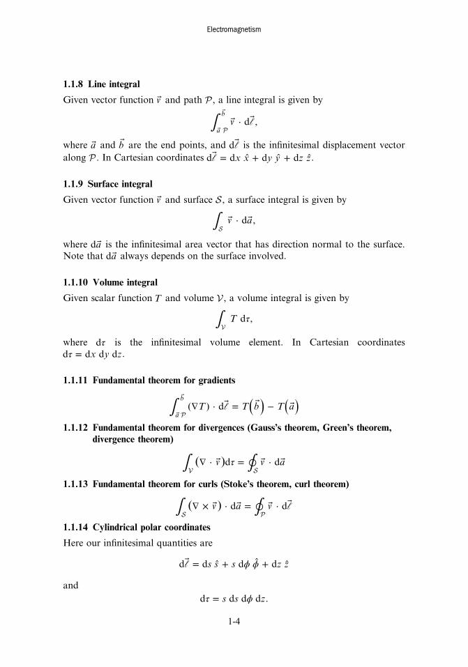
1.1.8 Line integral
Given vector function v and path P , a line integral is given by
Pl∫ ⋅
v d ,
a
b
where a and b are the end points, and ld is the infinitesimal displacement vectoralong P . In Cartesian coordinates l = ˆ + ˆ + ˆx x y y z zd d d d .
1.1.9 Surface integral
Given vector function v and surface S , a surface integral is given by
S∫ ⋅ v ad ,
where ad is the infinitesimal area vector that has direction normal to the surface.Note that ad always depends on the surface involved.
1.1.10 Volume integral
Given scalar function T and volume V , a volume integral is given by
V∫ τT d ,
where τd is the infinitesimal volume element. In Cartesian coordinatesτ = x y zd d d d .
1.1.11 Fundamental theorem for gradients
Pl∫ ∇ ⋅ = −
( ) ( )T T b T a( ) da
b
1.1.12 Fundamental theorem for divergences (Gauss’s theorem, Green’s theorem,divergence theorem)
V S∫ ∮τ∇ ⋅ = ⋅ ( )v v ad d
1.1.13 Fundamental theorem for curls (Stoke’s theorem, curl theorem)
S Pl∫ ∮∇ × ⋅ = ⋅ ( )v a vd d
1.1.14 Cylindrical polar coordinates
Here our infinitesimal quantities are
l ϕ ϕ = ˆ + ˆ + ˆs s s z zd d d d
andτ ϕ= s s zd d d d .
Electromagnetism
1-4

1.1.15 Spherical polar coordinates
Here our infinitesimal quantities are
l θ θ θ ϕ ϕ = ˆ + ˆ + ˆr r r rd d d sin d
and
τ θ θ ϕ= r rd sin d d d .2
1.1.16 One-dimensional Dirac delta function
The one-dimensional Dirac delta function is given by
δ − = ≠∞ =
⎧⎨⎩x ax ax a
( )0
and has the following properties
∫ δ − =−∞
∞
x a x( )d 1
∫ δ − =−∞
∞
f x x a x f a( ) ( )d ( )
δ δ=kxk
x( )1
( ).
1.1.17 Theory of vector fields
If the curl of a vector field F vanishes everywhere, then F can be written as thegradient of a scalar potentialV :
∇ × ↔ = −∇F F V .
If the divergence of a vector vanishes everywhere, then F can be expressed as the curlof a vector potential A:
∇ ⋅ = ↔ = ∇ × F F A0 .
1.2 Problems and solutionsProblem 1.1. Given vectors = ˆ + ˆ + ˆA x y z3 9 5 and = ˆ − ˆ + ˆB x y z7 4 , calculate
⋅ A B and × A B using vector components and find the angle between A and Busing both products.
Electromagnetism
1-5

Solution
⋅ = ˆ + ˆ + ˆ ⋅ ˆ − ˆ + ˆ
= + − + = − +
⋅ = −
× =ˆ ˆ ˆ
−
= − − ˆ + − ˆ + − − ˆˆ × ˆ = ˆ − ˆ − ˆ
A B x y z x y z
A B
A Bx y z
x y z
A B x y z
(3 9 5 ) ( 7 4 )
(3)(1) (9)( 7) (5)(4) 3 63 20
40
3 9 51 7 4
[(9)(4) ( 7)(5)] [(1)(5) (3)(4)] [(3)( 7) (1)(9)]
71 7 30
To find the angle θ between A and B we must first calculate A and B:
= + + =
= + − + =
A
B
3 9 5 115
1 ( 7) 4 66 .
2 2 2
2 2 2
Using the dot product, we have
θ θ
θ
⋅ = → = −
= °
−⎛⎝⎜
⎞⎠⎟A B AB cos cos
40
115 66117.3 .
1
Using the cross product, we have
θ θ
θ
× = → + − + − =
= °
A B AB sin 71 ( 7) ( 30) 115 66 sin
62.7 .
2 2 2
Note, however, that we can see that the angle between A and B is greater than °90 .For any argument γ , γ− ° ⩽ ⩽ °−90 sin ( ) 901 . Since the angle between A and B isgreater than °90 , we must adjust for this by subtracting our angle from °180 .Therefore, θ = ° − ° = °180 62.7 117.3 as expected.
Electromagnetism
1-6

Problem 1.2. The scalar triple product states ⋅ × = ⋅ × A B C B C A( ) ( ). Provethis by expressing each side in terms of its components.
Solution Starting with the left-hand side, the cross product is
× =ˆ ˆ ˆ
= − ˆ + − ˆ + − ˆ( )( ) ( )
B C
x y zB B B
C C C
B C B C x B C B C y B C B C z.
x y z
x y z
y z z y z x x z x y y x
Now, dotting A with × B C( )
⋅ × = − + − + −
= − + − + −
= − + − + −
⋅ × = ⋅ − ˆ + − ˆ + − ˆ⎡⎣ ⎤⎦
( )
( )
( )
( ) ( ) ( )
( ) ( )
( ) ( ) ( )
A B C A B C B C A B C B C A B C B C
A B C A B C A B C A B C A B C A B C
B C A C A B C A C A B C A C A
A B C B C A C A x C A C A y C A C A z .
x y z z y y z x x z z x y y x
x y z x z y y z x y x z z x y z y x
x y z z y y z x x z z x y y x
y z z y z x x z x y y x
Note the term in brackets is precisely × C A, therefore
⋅ × = ⋅ × ( ) ( )A B C B C A
as desired. This procedure can easily be applied again to prove the final part of thetriple product,
⋅ × = ⋅ × = ⋅ × ( ) ( ) ( )A B C B C A C A B .
Problem 1.3. Given source vector θ θ′ = ˆ + ˆr r x r ycos sin and field vector = ˆr zz,find the separation vector r and the unit vector rˆ.
Solution We have
r
r
θ θ
θ θ
= − ′ = ˆ − ˆ + ˆ
= − ˆ − ˆ + ˆ( )r r zz r x r y
r x r y zz
cos sin
cos sin .
To determine the unit vector rˆ, we must first find the magnitude of r ,
r θ θ θ θ= − + − + = + + = +( )r r z r z r z( cos ) ( sin ) cos sin .2 2 2 2 2 2 2 2 2
Electromagnetism
1-7

So
r rr
θ θˆ =
= − ˆ − ˆ + ˆ+
r x r y zz
r z
cos sin.
2 2
Problem 1.4. Given A in coordinate system K, find the rotational matrix to give thecomponents in system ′K .
Solution From the figures, we have
′ = ′ = ′ = −A A A A A A, , .x y y x z z
We want to find the rotational matrix R that satisfies
′
′
′
=
⎛
⎝
⎜⎜⎜⎜
⎞
⎠
⎟⎟⎟⎟
⎛
⎝⎜⎜⎜
⎞
⎠⎟⎟⎟
A
A
A
RAA
A.
x
y
z
x
y
z
From our equations above
′
′
′
=−
⎛
⎝
⎜⎜⎜⎜
⎞
⎠
⎟⎟⎟⎟
⎛
⎝⎜⎜⎜
⎞
⎠⎟⎟⎟
⎛
⎝⎜⎜⎜
⎞
⎠⎟⎟⎟
A
A
A
AA
A
0 1 0
1 0 0
0 0 1
.
x
y
z
x
y
z
Electromagnetism
1-8

Therefore,
=−
⎛
⎝⎜⎜⎜
⎞
⎠⎟⎟⎟R
0 1 0
1 0 0
0 0 1
.
Problem 1.5. Find the gradient of the following functions:a) = + +T x y z4 2 3
b) =T x y zln2 3
c) = +T x y z2 3
Solutionsa) = + +T x y z4 2 3
∇ = ∂∂
ˆ + ∂∂
ˆ + ∂∂
ˆ = ˆ + ˆ + ˆTTx
xTy
yTz
z x x yy z z4 2 33 2
b) =T x y zln2 3
∇ = ∂∂
ˆ + ∂∂
ˆ + ∂∂
ˆ = ˆ + ˆ + ˆTTx
xTy
yTz
z xz y xx z
yy x z y z2 ln 3 ln3
2 32 2
c) = +T x y z2 3
∇ = ∂∂
ˆ + ∂∂
ˆ + ∂∂
ˆ = ˆ + ˆ + ˆTTx
xTy
yTz
z xyx x y z z2 32 2
Problem 1.6. Find the divergence of the following functions:a) = ˆ − ˆ + ˆv xyx y zy z z2 2 3
b) = + ˆ + + ˆ + + ˆv x y x y z y z x z( ) ( ) ( )
Solutionsa) = ˆ − ˆ + ˆv xyx y zy z z2 2 3
∇ ⋅ = ∂∂
+∂∂
+ ∂∂
= − +vvx
v
yvz
y yz z4 3x y z 2
b) = + ˆ + + ˆ + + ˆv x y x y z y z x z( ) ( ) ( )
∇ ⋅ = ∂∂
+∂∂
+ ∂∂
= + + =vvx
v
yvz
1 1 1 3x y z
Problem 1.7. Find the curl of the following functions:a) = ˆ − ˆ + ˆv xyx y zy z z2 2 3
b) = + ˆ + + ˆ + + ˆv x y x y z y z x z( ) ( ) ( )c) = ˆ + ˆv x x y ysin cos
Electromagnetism
1-9

Solutionsa) = ˆ − ˆ + ˆv xyx y zy z z2 2 3
∇ × = ∂∂
−∂∂
ˆ + ∂∂
− ∂∂
ˆ +∂∂
− ∂∂
ˆ
= ∂∂
−∂ −
∂ˆ +
∂∂
−∂
∂ˆ
+∂ −
∂−
∂∂
ˆ
= + ˆ + − ˆ + − ˆ
∇ × = ˆ − ˆ
⎜ ⎟⎛⎝⎜
⎞⎠⎟
⎛⎝
⎞⎠
⎛⎝⎜
⎞⎠⎟
⎡
⎣⎢⎢
⎤
⎦⎥⎥
⎡
⎣⎢⎢
⎤
⎦⎥⎥
⎡
⎣⎢⎢
⎤
⎦⎥⎥
( ) ( )
( )
( )
vvy
v
zx
vz
vx
yv
xvy
z
zy
y z
zx
xy
z
z
xy
y z
x
xy
yz
y x y x z
v y x xz
( ) 2 ( )
2 ( )
0 2 (0 0) (0 )
2
z y x z y x
3 2 3
2
2
2
b) = + ˆ + + ˆ + + ˆv x y x y z y z x z( ) ( ) ( )
∇ × = ∂∂
−∂∂
ˆ + ∂∂
− ∂∂
ˆ +∂∂
− ∂∂
ˆ
= ∂ +∂
− ∂ +∂
ˆ + ∂ +∂
− ∂ +∂
ˆ
+ ∂ +∂
− ∂ +∂
ˆ
∇ × = − ˆ − ˆ − ˆ
⎜ ⎟⎛⎝⎜
⎞⎠⎟
⎛⎝
⎞⎠
⎛⎝⎜
⎞⎠⎟
⎡⎣⎢
⎤⎦⎥
⎡⎣⎢
⎤⎦⎥
⎡⎣⎢
⎤⎦⎥
vvy
v
zx
vz
vx
yv
xvy
z
z xy
y zz
xx y
zz x
xy
y zx
x yy
z
v x y z
( ) ( ) ( ) ( )
( ) ( )
z y x z y x
c) = ˆ + ˆv x x y ysin cos
∇ × = ∂∂
−∂∂
ˆ + ∂∂
− ∂∂
ˆ +∂∂
− ∂∂
ˆ⎜ ⎟⎛⎝⎜
⎞⎠⎟
⎛⎝
⎞⎠
⎛⎝⎜
⎞⎠⎟v
vy
v
zx
vz
vx
yv
xvy
zz y x z y x
= ∂∂
− ∂∂
ˆ + ∂∂
− ∂∂
ˆ
+ ∂∂
− ∂∂
ˆ =
⎡⎣⎢
⎤⎦⎥
⎡⎣⎢
⎤⎦⎥
⎡⎣⎢
⎤⎦⎥
yy
zx
xz x
y
yx
xy
z
(0) (cos ) (sin ) (0)
(cos ) (sin )0
Electromagnetism
1-10

Problem 1.8. Prove ∇ × ∇ =T( ) 0.
Solution
∇ × ∇ =
ˆ ˆ ˆ
∂∂
∂∂
∂∂
∂∂
∂∂
∂∂
( )T
x y z
x y z
Tx
Ty
Tz
= ∂∂
∂∂
− ∂∂
∂∂
ˆ + ∂∂
∂∂
− ∂∂
∂∂
ˆ
+ ∂∂
∂∂
− ∂∂
∂∂
ˆ
⎜ ⎟ ⎜ ⎟ ⎜ ⎟
⎜ ⎟
⎡⎣⎢
⎛⎝
⎞⎠
⎛⎝⎜
⎞⎠⎟⎤⎦⎥
⎡⎣⎢
⎛⎝
⎞⎠
⎛⎝
⎞⎠⎤⎦⎥
⎡⎣⎢
⎛⎝⎜
⎞⎠⎟
⎛⎝
⎞⎠⎤⎦⎥
yTz z
Ty
xz
Tx x
Tz
y
xTy y
Tx
z
∇ × ∇ =T( ) 0.
Problem 1.9. Find the Laplacian of the following functions:a) = + + +T x y xz 32
b) = +T y ze sin cos(2 )x
c) =T x ysin cosd) = ˆ + ˆ − ˆv xyx z y z22
Solutionsa) = + + +T x y xz 32
∇ = ∂∂
+ ∂∂
+ ∂∂
= + + =TT
xT
yTz
0 2 0 222
2
2
2
2
2
b) = +T y ze sin cos(2 )x
∇ = ∂∂
+ ∂∂
+ ∂∂
= − −
= −
TT
xT
yTz
y z y z
y z
e sin cos(2 ) 4 sin cos(2 )
e 5 sin cos(2 )
x
x
22
2
2
2
2
2
c) =T x ysin cos
∇ = ∂∂
+ ∂∂
+ ∂∂
= − − = −TT
xT
yTz
x y x y x ysin cos sin cos 2 sin cos22
2
2
2
2
2
Electromagnetism
1-11

d) = ˆ + ˆ − ˆv xyx z y z22
∇ = ∂∂
+ ∂∂
+ ∂∂
ˆ +∂∂
+∂∂
+∂∂
ˆ
+ ∂∂
+ ∂∂
+ ∂∂
ˆ
⎛⎝⎜
⎞⎠⎟
⎛⎝⎜
⎞⎠⎟
⎛⎝⎜
⎞⎠⎟
vv
xv
yvz
xv
x
v
y
v
zy
vx
vy
vz
z
x x x y y y
z z z
22
2
2
2
2
2
2
2
2
2
2
2
2
2
2
2
2
2
∇ = + + ˆ + + + ˆ+ + + ˆ = ˆv x y z y(0 0 0) (0 0 2) (0 0 0) 22
Problem 1.10. Test the divergence theorem with = ˆ + ˆ + − ˆv xyx y z y x z y z2 ( 2 )2 3 2
and the volume below.
Solution The divergence theorem states
V S∫ ∮τ∇ ⋅ = ⋅ v v ad d .
Starting with the left-hand side, we have the divergence
∇ ⋅ = + + = + +( )v y yz x y z x2 2 2 1 .3 2 3 2
We must split the volume into two pieces, (a) ⩽ ⩽y0 1 and (b) ⩽ ⩽y1 2.(a)
∫ ∫ ∫ ∫∇ ⋅ τ = + + =⎡⎣ ⎤⎦( )v y z x y x zd 2 1 d d d523
0
2
0
2
0
1
3 2
Electromagnetism
1-12
(b)
∫ ∫ ∫ ∫∇ ⋅ τ = + + =− ⎡⎣ ⎤⎦( )v y z x y x zd 2 1 d d d
17615
y
0
2
1
2
0
4 2
3 2
So,
V∫ ∇ ⋅ τ = + =v d
523
17615
43615
.
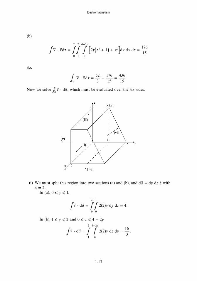
Now we solveS
∮ ⋅ v ad , which must be evaluated over the six sides.
(i) We must split this region into two sections (a) and (b), and = ˆa y z zd d d with=x 2.In (a), ⩽ ⩽y0 1,
∫ ∫ ∫ ⋅ = =v a y y zd 2(2) d d 4.0
2
0
1
In (b), ⩽ ⩽y1 2 and ⩽ ⩽ −z y0 4 2
∫ ∫ ∫ ⋅ = =−
v a y z yd 2(2) d d163
.
y
1
2
0
4 2
Electromagnetism
1-13

(ii) Here, = − ˆa y z xd d d and =x 0, so ⋅ = − ˆ =v a y y x xd 2(0) ( d d ) 0.(iii) Here, = ˆa x y zd d d and =z 2
∫ ∫ ∫ ⋅ = − =⎡⎣ ⎤⎦a x y xv d (2) 2y d d103
.0
2
0
1
2
(iv) Here, = − ˆa x y zd d d and =z 0
∫ ∫ ∫ ⋅ = − − =⎡⎣ ⎤⎦v a x y x yd (0) 2 ( d d ) 8.0
2
0
2
2
(v) Here = ˆa x z yd d d and =y 0, so ⋅ = − =v a z x zd 0 ( d d ) 02 3 .
(vi) Here, we have = ′ ˆa x z nd d d where ˆ = n nn. We can find n by crossing vectors
= − ˆ + ˆA y z2 and = ˆB x2 (the edges of the volume):
= × =ˆ ˆ ˆ
− = ˆ + ˆn A Bx y z
y z0 1 22 0 0
4 2 .
So
= + =n 4 2 2 52 2
and
ˆ = ˆ + ˆn y z2 5
55
5.
We can also obtain ′zd by considering
Electromagnetism
1-14

so ′ =z zd d52
. Now
= ˆ + ˆ = ˆ + ˆ⎛⎝⎜
⎞⎠⎟
⎛⎝⎜
⎞⎠⎟a x z y z y z x zd
52
d d2 5
55
512
d d
and
= − → = −z y yz
4 2 22
.
So
∫ ∫ ∫ ⋅ = + −⎡⎣⎢
⎤⎦⎥( )v a y z x z y x zd
12
2 d d0
2
0
2
2 3 2
∫ ∫= − + − − =⎜ ⎟ ⎜ ⎟⎧⎨⎩
⎛⎝
⎞⎠
⎡⎣⎢
⎛⎝
⎞⎠⎤⎦⎥⎫⎬⎭
zz x z
zx z2
212
2 22
d d425
.0
2
0
22
3 2
Therefore
S∮ ⋅ = + + + + =v ad 4
163
103
8425
43615
as expected.
Problem 1.11. Test the curl theorem with = ˆ + ˆ + ˆv xy x yz y x zz5 42 2 2 and the surfacebelow.
Electromagnetism
1-15

Solution The curl theorem states
S Pl∫ ∮∇ × ⋅ = ⋅ v a v( ) d d .
Starting with the left-hand side, the curl is given by
∇ × =
ˆ ˆ ˆ∂
∂∂∂
∂∂ = − ˆ − ˆ − ˆv
x y z
x y z
xy yz x z
yzx xzy xyz
5 4
2 8 10
2 2 2
We also have = ˆa y z xd d d with ⩽ ⩽ − − +z y0 ( 2) 42 . So
S∫ ∫ ∫∇ × ⋅ = − = −
− − +
v a yz z y( ) d 2 d d1024
15.
y
0
4
0
( 2) 42
Now to solveP
l∮ ⋅ v d over the two paths (i) and (ii):
(i) Here we have =x 0, =z 0, and l = ˆy yd d . So l ⋅ = =v y yd (0 )d 02 .(ii) Here we have l = ˆ + ˆy y z zd d d , =x 0, and = − − +z y( 2) 42
P Pl∫ ∫ ∫ ⋅ = + = − − + = −⎡⎣ ⎤⎦v yz y z z y y yd d 4(0 ) d ( 2) 4 d
102415
.4
0
2 2 2 2
Electromagnetism
1-16
So,
Pl∮ ⋅ = + − = −
v d 0102415
102415
as expected.
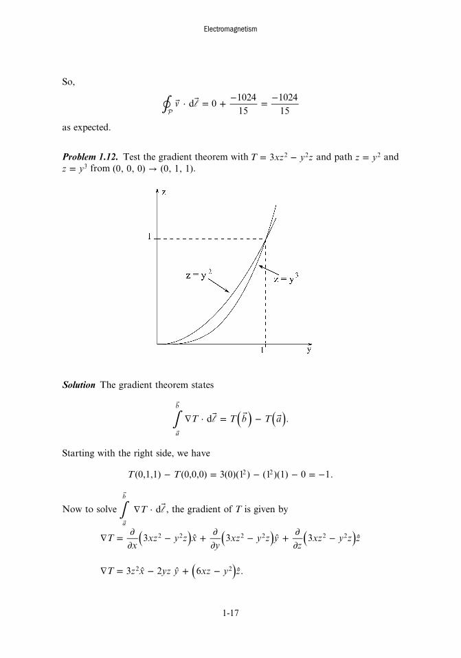
Problem 1.12. Test the gradient theorem with = −T xz y z3 2 2 and path =z y2 and=z y3 from →(0, 0, 0) (0, 1, 1).
Solution The gradient theorem states
l∫ ∇ ⋅ = −
( ) ( )T T b T ad .a
b
Starting with the right side, we have
− = − − = −T T(0,1,1) (0,0,0) 3(0)(1 ) (1 )(1) 0 1.2 2
Now to solve l∫ ∇ ⋅
T da
b
, the gradient of T is given by
∇ = ∂∂
− ˆ + ∂∂
− ˆ + ∂∂
− ˆ( ) ( ) ( )Tx
xz y z xy
xz y z yz
xz y z z3 3 32 2 2 2 2 2
∇ = ˆ − ˆ + − ˆ( )T z x yz y xz y z3 2 6 .2 2
Electromagnetism
1-17

Here, l = ˆ + ˆy y z zd d d with =x 0. So
l∇ ⋅ = − + − = − −⎡⎣ ⎤⎦T yz y z y z yz y y zd 2 d 6(0)( ) d 2 d d .2 2
For path (i), we have = → =z y z y yd 2 d2 . So
l∇ ⋅ = − − = −( )T y y y y y y y yd 2 d (2 d ) 4 d2 2 3
and
l∫ ∫∇ ⋅ = − = −
T y yd 4 d 1a
b
0
1
3
as expected. For path (ii), we have = → =z y z y yd 3 d3 2 . So
l∇ ⋅ = − − = −( ) ( )T y y y y y y y yd 2 d 3 d 5 d3 2 2 4
and
l∫ ∫∇ ⋅ = − = −
T y yd 5 d 1a
b
0
1
4
also as expected.
Problem 1.13. Verify the following integration by parts given =f xy z2 and = ˆ + ˆ − ˆA z x xyy x zz42 2 and the surface below,
S S Pl∫ ∫ ∮∇ × ⋅ = × ∇ ⋅ + ⋅ ⎡⎣ ⎤⎦( ) ( )f A a A f a fAd d d .
Electromagnetism
1-18

Solution Starting with the left-hand side
∇ × =
ˆ ˆ ˆ∂
∂∂∂
∂∂
−
= − − ˆ + ˆ = + ˆ + ˆA
x y z
x y z
z xy x z
z xz y yz z x y yz
4
[2 ( 2 )] 4 2 ( 1) 4 .
2 2
Now
∇ × = + ˆ + ˆ( )f A xy z x y xy zz2 ( 1) 4 .2 2 3
Here we have = ′ ˆa x z nd d d where ˆ = ˆ + ˆn x y and =n 2 so ˆ = ˆ + ˆn x y22
22
. Alsofrom
we have
′ = = −x x y xd 2 d with 1 .
Now
= ˆ + ˆ = ˆ + ˆ⎛⎝⎜
⎞⎠⎟ ( )a x z x y x z x yd 2 d d
22
22
d d .
Therefore,
S∫ ∫ ∫∇ × ⋅ = + ˆ + ˆ ⋅ ˆ + ˆ⎡⎣ ⎤⎦( )f A a xy z x y xy zz x y x zd 2 ( 1) 4 ( )d d
0
1
0
1
2 2 3
∫ ∫= − + =x x z x x z2 (1 ) ( 1)d d790
.0
1
0
1
2 2
Next, we will solve theP
l∮ ⋅ fA d term for the four segments.
Electromagnetism
1-19

Segment (i)
= → = =z f xy0 (0) 0.2
Segment (ii)
= → = =x f y z0 (0) 0.2
Segment (iii)
l = ˆ + ˆ = = − → = −x x y y z y x y xd d d , 1, and 1 d d .
Segment (iv)
= → = =y f x z0 (0 ) 0.2
So
l ⋅ = + = − − −⎡⎣ ⎤⎦( ) ( )f A xy z x xy y x x x x xd d 4 d (1 ) 1 4 (1 ) d2 2 2
and
Pl∮ ∫ ⋅ = − − − =⎡⎣ ⎤⎦fA x x x x xd (1 ) 1 4 (1 ) d
160
.0
1
2
Now to solve theS
∫ × ∇ ⋅ A f a[ ] d term. First, we have
∇ = ˆ + ˆ + ˆf y zx xyzy xy z2 .2 2
Electromagnetism
1-20

So
× ∇ =ˆ ˆ ˆ
−A f
x y z
z xy x z
y z xyz xy
( ) 4
2
2 2
2 2
= + ˆ + − − ˆ + − ˆ( ) ( ) ( )x y x yz x x y z xy z y xyz xy z z4 2 2 4 .2 3 3 2 2 2 2 2 2 3 3
As before, = ˆ + ˆa x z x yd d d ( ). So
S∫ ∫ ∫× ∇ ⋅ = − + −
− − − −
⎡⎣
⎤⎦
A f a x x x x z
x x z x x z x z
[ ( )] d 4 (1 ) 2 (1 )
(1 ) (1 ) d d0
1
0
1
2 3 3 2
2 2 2 2 2
S∫ × ∇ ⋅ =A f a[ ( )] d
11180
.
So
S Pl∫ ∮× ∇ ⋅ + ⋅ = + =A f a fA[ ( )] d d
11180
160
790
as expected.
Problem 1.14. Find the divergence and curl of the following functions:a) θ ϕ θ θ ϕ ϕ = ˆ + ˆ + ˆv r r cos sin sin cos2
b) ϕ ϕ ϕ ϕ ϕ = ˆ + ˆ+ ˆv s s z zcos cos sin sin
Solutionsa) θ ϕ θ θ ϕ ϕ = ˆ + ˆ + ˆv r r cos sin sin cos2
θ θθ
θ ϕ∇ ⋅ = ∂
∂+ ∂
∂+
∂∂θ
ϕ( ) ( )vr r
r vr
vr
v1 1sin
sin1
sinr2
2
θ θθ θ ϕ
θ ϕθ ϕ= ∂
∂+ ∂
∂+ ∂
∂( ) ( )r r
rr r
1 1sin
sin cos sin1
sin(sin cos )
24
ϕθ
θ θ ϕ= + − + + −( ) ( )r
rr r
14
sinsin
sin cos1
( sin )2
3 2 2
Electromagnetism
1-21

ϕθ
θ ϕ= + − −( )rr r
4sinsin
1 2 sinsin2
ϕ θ θ∇ ⋅ = + − −( )v rr
4sin
csc 2 sin 1
θ θθ
ϕ
θ ϕθ
θϕ
∇ × = ∂∂
− ∂∂
ˆ
+ ∂∂
− ∂∂
ˆ + ∂∂
− ∂∂
ˆ
ϕθ
ϕ θ
⎡⎣⎢
⎤⎦⎥
⎡⎣⎢
⎤⎦⎥
⎡⎣⎢
⎤⎦⎥
( )vr
vv
r
rv
rrv
r rrv
v
1sin
sin
1 1sin
( )1
( )r r
θ θθ ϕ
ϕθ ϕ
θ ϕθ ϕ θ
θ ϕϕ
ϕ
= ∂∂
− ∂∂
ˆ
+ ∂∂
− ∂∂
ˆ
+ ∂∂
− ∂∂
ˆ
⎡⎣⎢
⎤⎦⎥
⎡⎣⎢
⎤⎦⎥
⎡⎣⎢
⎤⎦⎥
( )
( )
( )
rr
rr
rr
r rr r
1sin
sin cos (cos sin )
1 1sin
( sin cos )
1( cos sin )
2
2
2
θθ θ ϕ θ ϕ θ ϕ θ
θ ϕ ϕ
= − ˆ − ˆ
+ ˆr
rr
r
1sin
(2 sin cos cos cos cos )sin cos
cos sin
θ ϕ θ θ ϕ θ θ ϕ ϕ∇ × = − ˆ − ˆ + ˆvr
rr r
cos cos(2 csc )
sin cos cos sin
b) ϕ ϕ ϕ ϕ ϕ = ˆ + ˆ + ˆv s s z zcos cos sin sin
ϕ∇ ⋅ = ∂
∂+
∂∂
+ ∂∂
ϕvs s
svs
v vz
1( )
1s
z
ϕϕ
ϕ ϕ ϕ= ∂∂
+ ∂∂
+ ∂∂( )
s ss
s zz
1cos
1(cos sin ) ( sin )2
ϕ ϕ ϕ ϕ= + − + +( )s
2 cos1
sin cos sin2 2
ϕ ϕ ϕ ϕ∇ ⋅ = + + −v
s2 cos sin
cos sin2 2
Electromagnetism
1-22

ϕϕ
ϕ∇ × = ∂
∂−
∂∂
ˆ + ∂∂
− ∂∂
ˆ + ∂∂
− ∂∂
ˆϕϕ⎜ ⎟
⎛⎝⎜
⎞⎠⎟
⎛⎝
⎞⎠
⎡⎣⎢
⎤⎦⎥v
sv v
zs
vz
vs s s
svv
z1 1
( )z s z s
ϕϕ ϕ ϕ ϕ ϕ ϕ
ϕ ϕϕ
ϕ
= ∂∂
− ∂∂
ˆ + ∂∂
− ∂∂
ˆ
+ ∂∂
− ∂∂
ˆ
⎡⎣⎢
⎤⎦⎥
⎡⎣⎢
⎤⎦⎥
⎡⎣⎢
⎤⎦⎥
sz
zs
zs
sz
s ss s z
1( sin ) (cos sin ) ( cos ) ( sin )
1( cos sin ) ( cos )
ϕ ϕ ϕ ϕ= ˆ + + ˆzs
ss
s zcos1
(cos sin sin )
ϕ ϕ ϕ∇ × = ˆ + + ˆvzs
ss
s zcossin
(cos )
Problem 1.15. Find the gradient and Laplacian of:a) θ ϕ θ ϕ= +T r (cos sin sin cos )2
b) ϕ ϕ= −T z ssin cos2 2
Solutionsa) θ ϕ θ ϕ= +T r (cos sin sin cos )2
θθ
θ ϕϕ∇ = ∂
∂ˆ + ∂
∂ˆ + ∂
∂ˆT
Tr
rr
Tr
T1 1sin
θ ϕ θ ϕ θ ϕ θ ϕ θ
θθ ϕ θ ϕ ϕ
= + ˆ + − + ˆ
+ − ˆ
r rr
r
rr
2 (cos sin sin cos )1
( sin sin cos cos )
1sin
(cos cos sin sin )
2
2
θ ϕ θ ϕ θ ϕ θ ϕ θ
θθ ϕ θ ϕ ϕ
= + ˆ + − ˆ
+ − ˆ
r r r
r
2 (cos sin sin cos ) (cos cos sin sin )
sin(cos cos sin sin )
θ ϕ θ ϕ θθ
θ ϕ ϕ∇ = + ˆ + + ˆ + + ˆT r r rr
2 sin( ) cos( )sin
cos( ) .
Note we could have written T as θ ϕ= +T r sin( )2 and then computed thegradient.
θ θθ
θ θ ϕ∇ = ∂
∂∂∂
+ ∂∂
∂∂
+ ∂∂
⎜ ⎟ ⎜ ⎟⎛⎝
⎞⎠
⎛⎝
⎞⎠
⎛⎝⎜
⎞⎠⎟T
r rr
Tr r
Tr
T1 1sin
sin1
sin2
22
2 2 2
2
2
Electromagnetism
1-23
θ ϕθ θ
θ θ ϕ
θ ϕθ ϕ
= ∂∂
+ + ∂∂
+
+ ∂∂
+
⎡⎣ ⎤⎦ ⎡⎣ ⎤⎦⎡⎣ ⎤⎦
r rr
rr
rr
12 sin( )
1sin
sin cos( )
1sin
cos( )
23
22
2 22
θ ϕθ
θ θ ϕ θ θ ϕ
θθ ϕ
= + + + − +
+ − +( )
[ ]6 sin( )1
sincos cos( ) sin sin( )
1sin
sin( )2
θ ϕ θθ
θ ϕ θ ϕθ
∇ = + + + − +T 5 sin( )
cossin
cos( )sin( )
sin.2
2
b) ϕ ϕ= −T z ssin cos2 2
ϕϕ∇ = ∂
∂ˆ + ∂
∂ˆ + ∂
∂ˆT
Ts
ss
T Tz
z1
ϕ ϕϕ
ϕ ϕ ϕ
ϕ ϕ
= ∂∂
− ˆ + ∂∂
− ˆ
+ ∂∂
− ˆ
( ) ( )
( )s
z s ss
z s
zz s z
sin cos1
sin cos
sin cos
2 2 2 2
2 2
ϕ ϕ ϕ ϕ ϕ ϕ= − ˆ + − − ˆ + ˆ⎡⎣ ⎤⎦ss
z s z zcos1
cos 2 cos ( sin ) 2 sin2 2
ϕ ϕ ϕ ϕ ϕ∇ = − ˆ + + ˆ + ˆ( )T ss
z s z zcoscos
2 sin 2 sin2 2
ϕ∇ = ∂
∂∂∂
+ ∂∂
+ ∂∂
⎜ ⎟⎛⎝
⎞⎠T
s ss
Ts s
T Tz
1 122
2
2
2
2
ϕ ϕ ϕ∂∂
= − → ∂∂
= − → ∂∂
∂∂
= −⎜ ⎟⎛⎝
⎞⎠
Ts
sTs
ss
sTs
cos cos cos2 2 2
ϕϕ ϕ ϕ
ϕϕ ϕ ϕ∂
∂= + → ∂
∂= − + − +( )T
z sT
z scos 2 cos sin sin 2 sin cos22
22 2 2
ϕ ϕ∂∂
= → ∂∂
=Tz
zTz
2 sin 2 sin2
ϕ ϕ ϕ ϕ ϕ∇ = − + − + − +( )Ts s
zs
cos 2sin cos sin 2 sin2
22 2
2
2
Electromagnetism
1-24
ϕ ϕ ϕ∇ = − + −⎛⎝⎜
⎞⎠⎟T
s szs
cos 2sin 2 sin2
22
2
2
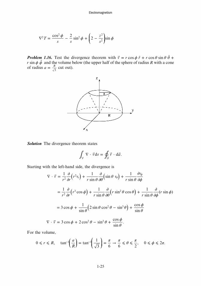
Problem 1.16. Test the divergence theorem with ϕ θ θ θ = ˆ + ˆ +v r r rcos cos sinϕ ϕr sin and the volume below (the upper half of the sphere of radius R with a cone
of radius =a R
3cut out).
Solution The divergence theorem states
V S∫ ∮τ∇ ⋅ = ⋅ v v ad d .
Starting with the left-hand side, the divergence is
θ θθ
θ ϕ∇ ⋅ = ∂
∂+ ∂
∂+
∂∂θ
ϕ( ) ( )vr r
r vr
vr
v1 1sin
sin1
sinr2
2
ϕθ θ
θ θθ ϕ
ϕ= ∂∂
+ ∂∂
+ ∂∂( ) ( )
r rr
rr
rr
1cos
1sin
sin cos1
sin( sin )
23 2
ϕθ
θ θ θ ϕθ
= + − +( )3 cos1
sin2 sin cos sin
cossin
2 3
ϕ θ θ ϕθ
∇ ⋅ = + − +v 3 cos 2 cos sincossin
.2 2
For the volume,
π π θ π ϕ π⩽ ⩽ = = → ⩽ ⩽ ⩽ ⩽− −⎜ ⎟⎛⎝
⎞⎠
⎛⎝⎜
⎞⎠⎟r R
aR
0 , tan tan1
3 6 6 2, 0 2 .1 1
Electromagnetism
1-25

So
V∫ ∫ ∫ ∫τ ϕ θ θ ϕ
θθ ϕ θ∇ ⋅ = + − +
π
ππ
⎜ ⎟⎛⎝
⎞⎠( )v r rd 3 cos 2 cos sin
cossin
sin d d d
R
06
2
0
2
2 2 2
V∫ τ π∇ ⋅ = −v Rd
312
.3
Now for the right-hand side, we have three surfaces: the bottom (i), the outer shell(ii), and the inner part where the cone is cut out (iii). We have
ϕ ϕ ϕ θ θ θ = ˆ + ˆ + ˆv r r r rcos sin cos sin .
For (i), we have ϕ θ = ˆa r rd d d and θ = π2. So
π π ϕ ⋅ = =v a r rd cos2
sin2
d d 02
and
∫ ⋅ =v ad 0.i( )
For (ii), we have =r R and θ θ ϕ θ θ ϕ = ˆ = ˆa r r R rd sin d d sin d d2 2 . So
ϕ θ θ ϕ ⋅ =v a Rd cos sin d d3
and
∫ ∫ ∫ ϕ θ θ ϕ ⋅ = =π
π
π
v a Rd cos sin d d 0.ii( ) 0
2
6
23
For (iii), we have θ = π6and θ ϕ θ ϕ θ = − ˆ = − ˆa r r r rd sin d d d d1
2. So
π π ⋅ = − = −v a r rd12
cos6
sin6
38
2 2
and
∫ ∫ ∫ ϕ π ⋅ = − = −π
v a r r Rd3
8d d
312
.iii
R
( ) 0 0
2
2 3
Electromagnetism
1-26

Therefore,
S∮ π ⋅ = −v a Rd
312
3
as expected.
Problem 1.17. Test the curl theorem with ϕ ϕ ϕ ϕ = ˆ + ˆ + ˆv s z s zs zsin cos cos2
and half of a cylindrical shell with radius R and height h.
Solution The curl theorem states
S Pl∫ ∮∇ × ⋅ = ⋅ ( )v a vd d .
Starting with the left-handed side, we have
ϕ ϕ = ˆ = ˆa s z s R z sd d d d d .
Since we are dotting ad with ∇ × v , we only need the s component of the curl:
ϕ ϕϕ ϕ ϕ
ϕ
∇ × = ∂∂
−∂∂
ˆ = ∂∂
− ∂∂
ˆ
= − ˆ
ϕ⎛⎝⎜
⎞⎠⎟
⎡⎣⎢
⎤⎦⎥v
sv v
zs
szs
zs
z s
[ ]1 1
( cos ) (sin cos )
sin .
sz
So
ϕ ϕ∇ × ⋅ = −( )v a Rz zd sin d d .
Electromagnetism
1-27

We have
ϕ π⩽ ⩽ ⩽ ⩽z h0 and 0
so
S∫ ∫ ∫ ϕ ϕ∇ × ⋅ = − = −
π
( )v a Rz z h Rd sin d d .
h
0 0
2
For the left-hand side, we have four curves
with
ϕ ϕ ϕ ϕ = ˆ + ˆ + ˆv s z s z zsin cos cos .2
For curve (i), l ϕ ϕ = ˆd d , =z 0, and =s R. So
l ϕ ϕ ϕ ⋅ =v d sin cos d
and
∫ ϕ ϕ ϕ =π
sin cos d 0.0
For curve (ii), l = ˆz zd d , ϕ π= , and =s R. So
l ϕ π ⋅ = = = −v zs z zR z zR zd cos d cos d d
and
∫ − = −zR z h Rd12
.
h
0
2
Electromagnetism
1-28

For curve (iii), l ϕ ϕ = ˆd d , =z h, and =s R. So
l ϕ ϕ ϕ ⋅ =v d sin cos d
and
∫ ϕ ϕ ϕ =π
sin cos d 0.
0
For curve (iv), l = ˆz zd d , ϕ = 0, and =s R. So
l ϕ ⋅ = = =v zs z zR z zR zd cos d cos(0)d d
and
∫ = −zR z h Rd12
.h
0
2 2
So,
P
l∮ ⋅ = − − = −v h R h R h Rd12
12
2 2 2
as expected.
Problem 1.18. Test the gradient theorem using ϕ=T sz sin2 and the half helix path(radius R, height h).
Electromagnetism
1-29

Solution The gradient theorem states
Pl∫ ∇ ⋅ = − ( ) ( )T T b T ad .
Starting with the right-hand side
π π π π − = − − = − − =⎜ ⎟ ⎜ ⎟ ⎜ ⎟⎛⎝
⎞⎠
⎛⎝
⎞⎠
⎛⎝
⎞⎠( ) ( )T b T a T R h T R Rh R h R,
2, ,
2, 0 sin
2(0) sin
2.2 2 2
Now, the gradient is
ϕϕ ϕ ϕ ϕ ϕ∇ = ∂
∂ˆ + ∂
∂ˆ + ∂
∂ˆ = ˆ + ˆ + ˆT
Ts
ss
T Tz
z z s z sz z1
sin cos 2 sin .2 2
We also have =s R and l ϕ ϕ ϕ ϕ = ˆ + ˆ = ˆ + ˆs z z R z zd d d d . So
l ϕ ϕ ϕ∇ ⋅ = +T Rz Rz zd cos d 2 sin d .2
We need a way to relate z and ϕ. Note that as ϕ increases, z increases linearly. So,using the equation of line
γ ϕ ϕ− = − )z z ( ,0 0
when =z 0 and ϕ = − π2,
γ ϕ π= +⎜ ⎟⎛⎝
⎞⎠z
2,
when =z h and ϕ = π2,
γ π π γπ
= + → =⎜ ⎟⎛⎝
⎞⎠h
h2 2
,
so
πϕ= −z
h h2
and
πϕ=z
hd d .
Using our expressions for z and zd , we have
lπ
ϕ ϕπ
ϕ ϕπ
ϕ∇ ⋅ = + + +⎡⎣⎢
⎛⎝⎜
⎞⎠⎟
⎛⎝⎜
⎞⎠⎟
⎛⎝⎜
⎞⎠⎟⎤⎦⎥T R
h hR
h h hd
2cos 2
2sin d .
2
So
l∫ ∫ πϕ ϕ
πϕ ϕ
πϕ∇ ⋅ = + + + =
π
π
−
⎡⎣⎢
⎛⎝⎜
⎞⎠⎟
⎛⎝⎜
⎞⎠⎟
⎛⎝⎜
⎞⎠⎟⎤⎦⎥T R
h hR
h h hh Rd
2cos 2
2sin d
a
b
2
2 22
as expected.
Electromagnetism
1-30

Problem 1.19. Evaluate the following integrals:
a) ∫ δ− + −x x x x(2 4) ( 2)d1
3
2
b) ∫ δ+ −−
x x x( 4) ( 2)d1
1
2
c) ∫ δ π−x xsin( ) ( )dx32
2
6
d) ∫ δ+−
x x x(2 1) (4 )d2
2
3
e) ∫ δ +−∞
∞
x x x(2 1)d2
f) ∫ δ −x b x( )d
a
0
Solutionsa)
∫ δ− + −( )x x x x2 4 ( 2)d .1
3
2
Since ∈2 (1, 3) and = − +f x x x( ) 2 42 , we have
∫ δ− + − = = − + =( )x x x x f2 4 ( 2)d (2) 2(2) 2 4 10.1
3
2 2
b)
∫ δ+ −−
( )x x x4 ( 2)d .1
1
2
Since ∉ −2 ( 1, 1), we have
∫ δ+ − =−
( )x x x4 ( 2)d 0.1
1
2
c)
∫ δ π−⎛⎝⎜
⎞⎠⎟
xx xsin
32
( )d .2
6
Electromagnetism
1-31

Since π ∈ (2, 6) and =f x( ) sin( )x32
, we have
∫ δ π π π− = = = −⎛⎝⎜
⎞⎠⎟
⎛⎝⎜
⎞⎠⎟
xx x fsin
32
( )d ( ) sin32
1.2
6
d)
∫ δ+−
( )x x x2 1 (4 )d .2
2
3
Since ∈ −0 ( 2, 2) and = +f x x( ) 2 13 , we have
∫ δ+ = = + =−
( ) ( )x x x f2 1 (4 )d14
(0)14
2(0) 114
.2
2
3 3
e)
∫ δ +−∞
∞
x x x(2 1)d .2
This can be rewritten as
∫ ∫ ∫δ δ δ+ = + = +−∞
∞
−∞
∞
−∞
∞⎡⎣⎢
⎛⎝⎜
⎞⎠⎟⎤⎦⎥
⎛⎝⎜
⎞⎠⎟x x x x x x x x x(2 1)d 2
12
d12
12
d .2 2 2
Since − ∈ −∞ ∞( , )12
and =f x x( ) 2, we have
∫ δ + = − = − =−∞
∞ ⎛⎝⎜
⎞⎠⎟
⎛⎝⎜
⎞⎠⎟
⎛⎝⎜
⎞⎠⎟x x x f
12
12
d12
12
12
12
18
.22
f)
∫ δ −x b x( )d .
a
0
Here we have
∫ δ − = < <{x b x b a( )d 1 if 00 otherwise
.
a
0
Problem 1.20. Suppose we have two vector fields = ˆF y z12 and = ˆ + ˆ + ˆF xx yy zz2 .
Calculate the divergence and curl of each. Which can be written as the gradient of ascalar and which can be written as the curl of a vector? Find a scalar and a vectorpotential.
Electromagnetism
1-32

Solution For F1, we have
∇ ⋅ = ∂∂
ˆ + ∂∂
ˆ + ∂∂
ˆ ⋅ ˆ =∂
∂=
⎛⎝⎜
⎞⎠⎟ ( )
( )F
xx
yy
zz y z
y
z01
22
and
∇ × =
ˆ ˆ ˆ∂
∂∂∂
∂∂ = ˆF
x y z
x y z
y
yx
0 0
2 .1
2
For F2, we have
∇ ⋅ = ∂∂
ˆ + ∂∂
ˆ + ∂∂
ˆ ⋅ ˆ + ˆ + ˆ = + + =⎛⎝⎜
⎞⎠⎟F
xx
yy
zz xx yy zz( ) 1 1 1 32
and
∇ × =
ˆ ˆ ˆ∂
∂∂∂
∂∂
= − ˆ + − ˆ + − ˆ =F
x y z
x y zx y z
x y z(0 0) (0 0) (0 0) 0.2
Since ∇ ⋅ =F 01 , F1 can be expressed as = ∇ × F A1 . We can find A by considering
∇ × =
ˆ ˆ ˆ∂
∂∂∂
∂∂
= ∂∂
−∂∂
ˆ + ∂∂
− ∂∂
ˆ +∂∂
− ∂∂
ˆ⎜ ⎟⎛⎝⎜
⎞⎠⎟
⎛⎝
⎞⎠
⎛⎝⎜
⎞⎠⎟
A
x y z
x y z
y
Ay
A
zx
Az
Ax
yA
xAy
z
0 0
.z y x z y x
2
By inspection:
∂∂
−∂∂
= ∂∂
− ∂∂
=∂∂
− ∂∂
=Ay
A
zAz
Ax
A
xAy
y0, 0, .z y x z y x 2
This is satisfied by
= ˆA y xy ,2
which is just one example. Since ∇ × =F 02 , F2 can be expressed as = −∇F V2 . Wecan findV by considering
Electromagnetism
1-33

= − ∂∂
ˆ + ∂∂
ˆ + ∂∂
ˆ⎛⎝⎜
⎞⎠⎟F
Vx
xVy
yVz
z .2
By inspection:
= −∂∂
= −∂∂
= −∂∂
xVx
yVy
zVz
, , .
This is satisfied by
= − + +⎛⎝⎜
⎞⎠⎟V
x y z2 2 2
2 2 2
which is again just one example.
BibliographyByron F W and Fuller R W 1992 Mathematics of Classical and Quantum Physics (New York:
Dover)Griffiths D J 1999 Introduction to Electrodynamics 3rd edn (Englewood Cliffs, NJ: Prentice Hall)Griffiths D J 2013 Introduction to Electrodynamics 4th edn (New York: Pearson)Halliday D, Resnick R and Walker J 2010 Fundamentals of Physics 9th edn (New York: Wiley)Halliday D, Resnick R and Walker J 2013 Fundamentals of Physics 10th edn (New York: Wiley)Purcell E M and Morin D J 2013 Electricity and Magnetism 3rd edn (Cambridge: Cambridge
University Press)Rogawski J 2011 Calculus: Early Transcendentals 2nd edn (San Francisco, CA: Freeman)
Electromagnetism
1-34