Embed Size (px)
Citation preview

ELECTROMAGNETICS
GENERAL THEORY OF THE
ELECTROMAGNETIC FIELD
CLASSICAL AND RELATIVISTIC APPROACHES
THIRD EDITION
Revised and Augmented
© 2012, Editura Universităţii Transilvania din Braşov Transilvania University Press, Braşov, 2012
Address: 500091 Braşov, RomaniaBd. Iuliu Maniu, nr. 41ATel.: 40-0268-476050Fax: 40-0268-476051
E-mail : [email protected]
Editură acreditată de CNCSISAdresa nr. 1615 din 29 mai 2002
Reviewers:
Jacques CURÉLYCentre de Physique MoléculaireOptique et Hertzienne (CPMOH)Université Bordeaux 1 – CNRSFrance
Dan BIDIANDepartment of Electrical Engineering and Applied PhysicsFaculty of Electrical Engineering and Computer ScienceTransilvania University of Braşov
Cover: Elisabeta GODGEA
ISBN 978-606-19-0113-5
Andrei NICOLAIDE
ELECTROMAGNETICS
GENERAL THEORY OF THE
ELECTROMAGNETIC FIELD
CLASSICAL AND RELATIVISTIC APPROACHES
THIRD EDITION
REVISED AND AUGMENTED
TRANSILVANIA UNIVERSITY PRESS
BRA OV – 2012

Author: Andrei NICOLAIDE Regular Member of the Academy of Technical Sciences in Romania
Distinguished University Professor
Life Senior Member of the IEEE (Institute of Electrical and Electronics Engineers)

PREFACE TO THE PRESENT EDITION The present book titled, Electromagnetics: General theory of the electromagnetic
field. Classical and relativistic approaches, is an extended form of the previous two editions of the books titled Electromagnetics: General theory of the electromagnetic field.
The new book, at the difference of the previous ones, contains four new appendices, devoted to several topics, as follows: a. A study on the divergence of tensors related to the curvature of the space-time continuum; b. The energy-momentum tensor of the electromagnetic field in the theory of relativity; c. The Sagnac effect in The General theory of relativity; d. A new approach to the calculation of the magnetic field strength of a solenoid and to the introduction of magnetic quantities.
In this book, apart from some improvements, new results have been included, some of them belonging to the author. These last ones have been presented at the ICAEM International Conference of Applied and Engineering Mathematics, held in London the last four years (2008-2011). The book will appear in both forms electronic and print.
The volume has been built in order to avoid the reader to resort to books of mathematics, all mathematical developments being included in the book.
The purpose of this book has been to present in a legible manner some important subjects of the concerned topics. At the same time, the text has been so prepared that a reader not interested in the Special Theory of Relativity and General Theory of Relativity could read it, avoiding the text connected with the relativistic treatment.
The book is devoted to all readers interested in these topics.
PREFACE TO THE FIRST EDITION
In the present work the physical fundamentals of electromagnetic phenomena are studied having in view their technical applications.
The book contains the general theory of the electromagnetic field necessary for the study of the principal applications in the following domains: Electrostatics, Electrokinetics, Electrodynamics and Magnetostatics.
The general theory contains the introduction (i.e., the definition) of fundamental concepts among which: field and substance, electric charge, electric current, state quantities of electric and magnetic fields, as well as the study of laws and energy of the electromagnetic field.
The general theory is presented in four chapters. Further, three appendices are added. For practical applications, the consideration of electromagnetic phenomena at a
macroscopic scale is of special interest. However, in many applications, it is necessary to know the phenomena at a microscopic scale.
At the same time, it is useful to have in view that the physical model is, in many cases, relatively simple in the case of a microscopic study. For this reason, in this work, the

Preface
6
following procedure has been used: The various quantities and phenomena have been first examined at a microscopic scale, and then, by calculating the average values, the passage to macroscopic quantities describing the phenomena has been accomplished.
Concerning the presentation of the general laws, there are, in principle, two possibilities:
a. The introduction of these laws directly, as a generalization of experimental facts; b. The derivation of these laws starting from the Coulomb law and the Special Theory
of Relativity. The Special Theory of Relativity has been used because it permits the derivation of the
equations of the theory of electromagnetic field starting from a small number of general equations.
Appendix 3, which contains the main formulae of the Special Theory of Relativity, and the derivation of certain relations between forces, given by the author, facilitates to follow the calculations of Chapters 2 and 3.
Also, some relatively recent considerations on the theory of relativity have been mentioned in Introduction.
The text has been elaborated so that all references to the special theory of relativity may be omitted; however, in this case, the number of basic general equations that are not derived from more general relations is greater.
The study of the mentioned domains, namely Electrostatics, Electrokinetics, Electrodynamics, Magnetostatics, can be carried out by using the general laws of electromagnetic field for these various cases. Certain important problems concerning the mentioned domains are analysed in the present work.
A more detailed study of the mentioned domains can be found in several works devoted to these subjects, including the works of the author, mentioned in Bibliography.
The system of units used in this work is the International System of Units (SI) and all formulae are written in this rationalized system.
This work differs to some extent from many other usual textbooks and works by the attention paid to certain subjects like the passage from the microscopic theory to the macroscopic one, the way of using the Special Theory of Relativity, and the simplicity of the presentation.
Certain parts of this work, especially those related to the Theory of Relativity, represent the content of the lectures of an extra-course given by the author at the Université Bordeaux 1 (France) in the summer semester of 2001.
The author thanks especially Doctors of Physics: Jean-Claude GIANDUZZO, Head of the Centre of Electrical and Electronic Resources, and Jacques CURÉLY, both from the Université Bordeaux 1 (France), for their support for the presentation of these lectures and for their valuable comments.
At the same time, the author wishes to thank Professor Florin Teodor TĂNĂSESCU, from the Polytechnica University of Bucharest, secretary general of the Academy of Technical Sciences in Romania, for his valuable support and suggestions.
Finally, the author should like to gratefully thank Dr. Phys. Jacques CURÉLY, from the Université Bordeaux 1, for the attention paid to the review of the manuscript and for his valuable comments and suggestions.
Andrei NICOLAIDE
CONTENTS
PREFACE . . . . . . . . . . . . . . . . . . . . . . . . . . . . . . . . . . 5 CONTENTS . . . . . . . . . . . . . . . . . . . . . . . . . . . . . . . . . 7 LIST OF SYMBOLS. . . . . . . . . . . . . . . . . . . . . . . . . . . . . 15 INTRODUCTION . . . . . . . . . . . . . . . . . . . . . . . . . . . . . . 23
1. Generalities on the Theory of the Electromagnetic Field and on the Structure of Substance . . . . . . . . . . . . . . . . . . . . . . . 31
1.1. Field and Substance . . . . . . . . . . . . . . . . . . . . . . . . . 31 1.2. Lines of Field. Tubes of Lines of Field. Equipotential Surfaces. Fluxes. . . . 32 1.2.1. Lines of Field. . . . . . . . . . . . . . . . . . . . . . . . . . . 32 1.2.2. Tubes of Field Lines. . . . . . . . . . . . . . . . . . . . . . . . 34 1.2.3. Equipotential Surface. . . . . . . . . . . . . . . . . . . . . . . . 34 1.2.4. Flux. . . . . . . . . . . . . . . . . . . . . . . . . . . . . . . 34 1.3. Physical Quantities. Laws and Theorems. . . . . . . . . . . . . . . . 36 1.4. Manners of Studying the Theory of the Electromagnetic Field . . . . . . . 38 1.4.1. The Macroscopic Study of the Electromagnetic Field . . . . . . . . . . . 38 1.4.2. The Microscopic Study of the Electromagnetic Field . . . . . . . . . . . 38 1.4.3. Generalities Concerning the Microscopic Study of the
Electromagnetic Field . . . . . . . . . . . . . . . . . . . . . . . . 38 1.4.4. Macroscopic Average (Mean) Values . . . . . . . . . . . . . . . . . 39 1.4.5. Manner of Studying Adopted in the Present Work . . . . . . . . . . . . 40 1.4.6. Laws of the Theory of Electric and Magnetic Phenomena . . . . . . . . . 40 1.5. General Considerations on the Structure of Conductors and Dielectrics. . . . 42 1.5.1. Electrically Conductive Materials . . . . . . . . . . . . . . . . . . . 42 1.5.2. Dielectrics . . . . . . . . . . . . . . . . . . . . . . . . . . . . . 42 1.6. Electric Charge. Electric Field Strength in Vacuo. . . . . . . . . . . . . 44 1.6.1. Electrification State. Electric Field. . . . . . . . . . . . . . . . . . . 44 1.6.2. True Electric Charge (Free Electric Charge) . . . . . . . . . . . . . . . 45 1.6.3. Density of Electric Charge . . . . . . . . . . . . . . . . . . . . . . 47 1.6.4. Conservation of the Free (True) Electric Charges. . . . . . . . . . . . . 48 1.6.5. The Electric Field Strength in Vacuo . . . . . . . . . . . . . . . . . . 48 1.6.6. The Macroscopic Electric Field Strength . . . . . . . . . . . . . . . . 49 1.7. Electric Field Strength in the Large Sense . . . . . . . . . . . . . . . . 52 1.8. Line-Integral (Circulation) of the Electric Field Strength along an Arc of Curve. Electric Potential Difference. Electric Tension, Voltage. Electromotive Force. . . . . . . . . . . . . . . . . . . . . . . . . 54 1.9. Polarization of Dielectrics . . . . . . . . . . . . . . . . . . . . . . 56 1.9.1. The Polarization Phenomenon of Dielectrics. Polarization State of
Dielectrics. Polarization Electric Charge (Bound Electric Charge). Electric Moment of a Neutral System of Electric Charges. . . . . . . . . . 56
1.9.2. The Macroscopic Electric Moment of a Polarized Body . . . . . . . . . . 58 1.9.3. The Polarization Electric Charge. Density of the Polarization Electric Charge. . . . . . . . . . . . . . . . . . . . . . . . . . . 59 1.9.4. Electric Polarization. . . . . . . . . . . . . . . . . . . . . . . . . 60 1.9.5. Polarization Electric Charge of the Interior of a Closed Surface in a Dielectric . . . . . . . . . . . . . . . . . . . . . . . . . . . 62 1.9.6. Ponderomotive Actions Exerted upon a Polarized Body in an Electric Field . . . . . . . . . . . . . . . . . . . . . . . . . . . 65

Contents 8
1.10. The Electric Current. . . . . . . . . . . . . . . . . . . . . . . . . 68 1.10.1. Electric Current Intensity. Electric Current Density. . . . . . . . . . . . 68 1.10.2. Conduction Electric Current . . . . . . . . . . . . . . . . . . . . . 72 1.10.3. Convection Electric Current . . . . . . . . . . . . . . . . . . . . . 72 1.10.4. Polarization Electric Current . . . . . . . . . . . . . . . . . . . . . 73 1.10.5. Amperian Electric Current (Molecular Electric Current) . . . . . . . . . . 76 1.11. Law of Free (True) Electric Charge Conservation . . . . . . . . . . . . 80 1.11.1. Integral Form of the Law. . . . . . . . . . . . . . . . . . . . . . . 80 1.11.2. Local Form of the Law . . . . . . . . . . . . . . . . . . . . . . . 80 1.12. The Law of Electric Conduction. The Local Form. . . . . . . . . . . . . 83 1.13. The Electric Field Strength of Electric Charges in Vacuo.
Electric Constant (Electric Permittivity of Vacuum) . . . . . . . . . . . 85 1.13.1. COULOMB Formula . . . . . . . . . . . . . . . . . . . . . . . . . 85 1.13.2. Utilization of the Principle of Superposition . . . . . . . . . . . . . . . 86 1.13.3. The Electric Potential Produced by Electric Charges at Rest . . . . . . . . 87 1.14. The Electric Flux Law in Vacuo . . . . . . . . . . . . . . . . . . . . 89 1.15. The SI Units of: Electric Charge, Electric Moment, Electric Tension, Electric Field Strength, Electric Current. . . . . . . . . . . . . . . . . 93 1.15.1. The Unit of Electric Charge . . . . . . . . . . . . . . . . . . . . . 93 1.15.2. The Unit of Electric Moment . . . . . . . . . . . . . . . . . . . . . 94 1.15.3. The Unit of Electric Tension . . . . . . . . . . . . . . . . . . . . . 94 1.15.4. The Unit of Electric Field Strength. . . . . . . . . . . . . . . . . . . 94 1.15.5. The Unit of Electric Current Intensity . . . . . . . . . . . . . . . . . 95
2. Introduction of the State Quantities of the Electromagnetic Field in Vacuo . . . . . . . . . . . . . . . . . . . . . . . . . . . . . 97
2.1. The Law of Ponderomotive Action upon a Point-like Electric Charge at Rest in an Inertial Reference Frame . . . . . . . . . . . . . . . . . . 97 2.2. Derivation of the Expression of the Law of Ponderomotive Action
upon a Point-like Charge That is Moving Relatively to an Inertial Reference Frame . . . . . . . . . . . . . . . . . . . . . . . . . 98 2.3. The Transformation Expression (When Passing from an Inertial
System to Another) of the Force in the Special Theory of Relativity . . . . . 99 2.3.1. The Transformation Expressions of Co-ordinates and Time . . . . . . . . 99 2.3.2. The Transformation Expressions of Forces . . . . . . . . . . . . . . . 104 2.3.3. The Manner of Adopting the Transformation Relations of Forces and Geometrical Quantities . . . . . . . . . . . . . . . . . . . . . . 105 2.4. The Expressions of the Force and Electric Field Strength in Various Reference
Frames. Electric Displacement in Vacuo and Magnetic Induction in Vacuo. Magnetic Constant (Magnetic Permeability
of Vacuum). . . . . . . . . . . . . . . . . . . . . . . . . . . . . 105 2.5. General Expressions of the Force Acting upon a Point-like Electric
Charge in Motion Relatively to an Inertial Reference Frame. Introduction (Definition) of the Quantities: Electric Field Strength E
and Magnetic Induction B. . . . . . . . . . . . . . . . . . . . . . . 109 2.6. The Magnetic Field. . . . . . . . . . . . . . . . . . . . . . . . . . 112 2.7. Transformation Relation of the Volume Density of the Free (True) Electric Charge. . . . . . . . . . . . . . . . . . . . . . . . . . . 113 2.8. The Expressions of the Magnetic Field Strength Produced at a Point
by a Moving Electric Charge or an Electric Current in Vacuo. The Biot-Savart-Laplace Formula. . . . . . . . . . . . . . . . . . . . 114
Contents 9
3. The Laws of the Electromagnetic Field . . . . . . . . . . . . . . . . . . 117 3.1. The Law of Electric Flux. . . . . . . . . . . . . . . . . . . . . . . 117 3.1.1. The Expression of the Law of Electric Flux in Vacuo . . . . . . . . . . . 117 3.1.2. The Expression of the Law of Electric Flux for Any Medium in the Case of Free (True) and Polarization Electric Charges . . . . . . . . 120 3.1.3. The General Expression of the Law of Electric Flux . . . . . . . . . . . 121 3.1.4. The Electric Flux through Various Surfaces . . . . . . . . . . . . . . . 122 3.2. The Relation between the Electric Displacement, Electric Field Strength and Electric Polarization . . . . . . . . . . . . . . . . . . . 122 3.3. The Law of Temporary Electric Polarization. . . . . . . . . . . . . . . 123 3.4. The Law of Magnetic Flux . . . . . . . . . . . . . . . . . . . . . . 125 3.4.1. The Expression of the Law of Magnetic Flux for Empty Space . . . . . . . 125 3.4.2. The Expression of the Law of Magnetic Flux for Any Medium . . . . . . . 126 3.4.3. The General Expression of the Law of Magnetic Flux (for Any Medium) . . . . . . . . . . . . . . . . . . . . . . . . . 127 3.4.4. The Magnetic Flux through Various Surfaces . . . . . . . . . . . . . . 128 3.4.5. The Magnetic Flux-turn. The Magnetic Flux-linkage. Magnetic Vector Potential. . . . . . . . . . . . . . . . . . . . . . . 129 3.5. The Law of Electromagnetic Induction for Media at Rest . . . . . . . . . 131 3.5.1. The Expression of the Law of Electromagnetic Induction for Empty Medium at Rest . . . . . . . . . . . . . . . . . . . . . . . 131 3.5.2. The Expression of the Law of Electromagnetic Induction
for Any Medium at Rest . . . . . . . . . . . . . . . . . . . . . . . 133 3.5.3. The General Expression of the Law of Electromagnetic
Induction for Media at Rest. . . . . . . . . . . . . . . . . . . . . . 134 3.5.4. The Concise Integral Form of the Expression of the Law of Electromagnetic Induction for Media at Rest. Faraday Law. . . . . . . . . 135 3.6. The Law of Magnetic Circuit (Magnetic Circuital Law) for Media at Rest . . . . . . . . . . . . . . . . . . . . . . . . . . 136 3.6.1. The Expression of the Law of Magnetic Circuit for Empty Medium at Rest . . . . . . . . . . . . . . . . . . . . . . . . . . 136 3.6.2. The General Expression of the Law of Magnetic Circuit for Empty
Medium at Rest . . . . . . . . . . . . . . . . . . . . . . . . . . 139 3.6.3. The Expression of the Law of Magnetic Circuit for Any Medium at
Rest, in the Presence of Free Electric Charges, Polarization Electric Charges and Amperian Currents. . . . . . . . . . . . . . . . . . . . 139
3.6.4. The General Expression of the Law of Magnetic Circuit for Any Medium at Rest . . . . . . . . . . . . . . . . . . . . . . . 142 3.6.5. Conditions (Regimes) of the Electromagnetic Field. Law of Magnetic Circuit in Quasi-stationary Condition. Ampère Law (Theorem). . . . . . . 143 3.6.6. The Components of the Magnetic Field Strength. Magnetic Tension. Magnetomotive Force. . . . . . . . . . . . . . . . . . . . . . . . . 144
3.6.7. The Concise Integral form of the Law of Magnetic Circuit for Media at Rest. . . . . . . . . . . . . . . . . . . . . . . 144 3.6.8. Adoption of the Curves and Surfaces That Occur in the Expressions of the Laws of Electromagnetic Induction, and Magnetic Circuit . . . . . . 147 3.7. The Relationship between Magnetic Induction, Magnetic Field Strength and Magnetic Polarization . . . . . . . . . . . . . . . . . . 147 3.8. The Law of Temporary Magnetization . . . . . . . . . . . . . . . . . 147 3.9. Derivation of the Fundamental Equations of the Electromagnetic
Field Theory in the General Case. Maxwell Equations. . . . . . . . . . . 150

Contents 10
3.10. Relations between the State Quantities of the Electromagnetic Field in Various Inertial Reference Frames . . . . . . . . . . . . . . . . . . 151 3.11. Expressions of the Laws of the Electromagnetic Induction and Magnetic Circuit for Moving Media . . . . . . . . . . . . . . . . . . 153 3.12. The Relations between the Components of the State Quantities of Electromagnetic Field in the Case of Discontinuity Surfaces . . . . . . . . 155 3.12.1. The Relation between the Normal Components of Electric
Displacement Vectors . . . . . . . . . . . . . . . . . . . . . . . . 156 3.12.2. The Relation between the Tangential Components of Electric Field Strength Vectors . . . . . . . . . . . . . . . . . . . . . . . . .157 3.12.3. The Theorem of Refraction of the Lines of Electric Field in the
Case of Insulating Media. . . . . . . . . . . . . . . . . . . . . . . 159 3.12.4. The Relation between the Normal Components of Magnetic Induction
Vectors . . . . . . . . . . . . . . . . . . . . . . . . . . . . . . 160 3.12.5. The Relation between the Tangential Components of the Magnetic
Field Strength Vectors . . . . . . . . . . . . . . . . . . . . . . . . 161 3.12.6. The Theorem of Refraction of the Lines of Magnetic Field at the
Passage through the Separation Surface of Two Media . . . . . . . . . . 163 3.12.7. The Relation between the Normal Components of Electric
Displacement Vectors and Electric Current Densities . . . . . . . . . . . 164 3.13. The SI Units of Measure of Electric and Magnetic Quantities:
Electric Flux, Electric Displacement, Electric Resistivity, Magnetic Flux, Magnetic Induction, Magnetic Field Strength. . . . . . . . 165
3.13.1. The Units of Electric Flux and Displacement . . . . . . . . . . . . . . 165 3.13.2. The Unit of Electric Resistivity . . . . . . . . . . . . . . . . . . . . 165 3.13.3. The Unit of Magnetic Flux . . . . . . . . . . . . . . . . . . . . . . 165 3.13.4. The Unit of Magnetic Induction . . . . . . . . . . . . . . . . . . . . 166 3.13.5. The Unit of Magnetic Field Strength . . . . . . . . . . . . . . . . . . 167 3.13.6. The Units of Electric and Magnetic Constant . . . . . . . . . . . . . . 167 3.13.7. Remarks on the Various Systems of Units of Measure
in Electromagnetism . . . . . . . . . . . . . . . . . . . . . . . . 168 3.14. The Laws of the Electromagnetic Field in the Case of Existence
of Magnetic Monopoles . . . . . . . . . . . . . . . . . . . . . . . 168 3.14.1. Expression of the Interaction Force between Two Magnetic Monopoles . . . . . . . . . . . . . . . . . . . . . . . . 169 3.14.2. Electric Field Produced by Moving Magnetic Monopoles . . . . . . . . . 170 3.14.3. The Expressions of the Laws of the Theory of the Electromagnetic Field in the Case of Magnetic Monopoles . . . . . . . . . . . . . . . 170 3.15. Application of the Biot-Savart-Laplace Formula to the Calculation
of the Magnetic Field Strength . . . . . . . . . . . . . . . . . . . . 170 3.15.1. Expression of the Magnetic Field Strength Produced by a
Thread-Like Rectilinear Conductor Carrying a Constant Electric Current . . . . . . . . . . . . . . . . . . . . . . . . . . 170
3.15.2. Expression of the Magnetic Field Strength Produced at a Point on the Axis of a Circular Turn Carrying a Constant Electric Current . . . . . . 173
3.16. Application of Both Forms of the Law of Electromagnetic Induction for Media at Rest and in Motion . . . . . . . . . . . . . . . . . . . 174
3.16.1. Calculation of the Electromotive Force Induced in a Coil in Rotational Motion in a Uniform Magnetic Field . . . . . . . . . . . . . 174
3.16.2. Calculation of the Electromotive Force Induced by the Rotation of a Magnet about its Axis . . . . . . . . . . . . . . . . . . . . . . 177

Contents 11
3.17. Electrodynamic Potentials . . . . . . . . . . . . . . . . . . . . . . 178 3.18. The Scalar and Vector Electrodynamic Potentials Produced by
One Electric Charge Moving at Constant Velocity . . . . . . . . . . . . 180 3.19. The Scalar and Vector Electrodynamic Potentials Produced by
One Point-like Electric Charge Moving at Non-constant Velocity . . . . . . 183
4. The Energy of the Electromagnetic Field . . . . . . . . . . . . . . . . . 189 4.1. The Expression of the Energy of the Electromagnetic Field.
Poynting Vector. . . . . . . . . . . . . . . . . . . . . . . . . . . 189 4.2. Theorem of Irreversible Transformation of Electromagnetic
Energy in the Case of Hysteresis Phenomenon . . . . . . . . . . . . . . 195 4.3. The Theorem of Irreversible Transformation of Electromagnetic
Energy Into Heat . . . . . . . . . . . . . . . . . . . . . . . . . . 195 4.4. The Theorem of Electromagnetic Momentum . . . . . . . . . . . . . . 196
APPENDICES . . . . . . . . . . . . . . . . . . . . . . . . . . . . . . . 203
APPENDIX 1 . . . . . . . . . . . . . . . . . . . . . . . . . . . . . . . 205 Vector Calculus . . . . . . . . . . . . . . . . . . . . . . . . . . . . . . 205
A.1.1. Vector Algebra . . . . . . . . . . . . . . . . . . . . . . . . . . . 205 A.1.2. Vector Analysis . . . . . . . . . . . . . . . . . . . . . . . . . . 208 A.1.2.1. Scalar and Vector Fields . . . . . . . . . . . . . . . . . . . . . . . 208 A.1.2.2. The Derivative of a Scalar Function in Regard to a Given Direction . . . . . 209 A.1.2.3. The Gradient . . . . . . . . . . . . . . . . . . . . . . . . . . . 210 A.1.2.4. The Flux of a Vector through a Surface . . . . . . . . . . . . . . . . 214 A.1.2.5. The Gauss and Ostrogradski Theorem. The Divergence of a Vector. . . . . 215 A.1.2.6. The Line-Integral of a Vector along a Curve. Circulation. . . . . . . . . . 219 A.1.2.7. The Stokes Theorem. The Curl of a Vector. . . . . . . . . . . . . . . . 219 A.1.2.8. Nabla Operator. Hamilton Operator. . . . . . . . . . . . . . . . . . . 224 A.1.2.9. The Derivative of a Vector Along a Direction . . . . . . . . . . . . . . 224 A.1.2.10. Expressing the Divergence and the Curl of a Vector by Means of the Nabla Operator . . . . . . . . . . . . . . . . . . . 226 A.1.2.11. Differential Operations by the Nabla Operator . . . . . . . . . . . . . 227 A.1.2.12. Integral Transformations Using the Nabla Operator . . . . . . . . . . . 230 A.1.2.13. Substantial Derivative of a Scalar with Respect to Time . . . . . . . . . 232 A.1.2.14. Substantial Derivative of a Volume Integral of a Scalar Function with
Respect to Time . . . . . . . . . . . . . . . . . . . . . . . . . . 233 A.1.2.15. Derivative with Respect to Time of the Flux through a Moving
Open Surface . . . . . . . . . . . . . . . . . . . . . . . . . . . 235
APPENDIX 2 . . . . . . . . . . . . . . . . . . . . . . . . . . . . . . . 239 Expressions of the Differential Operators in Curvilinear Co-ordinates . . . . . . 239
A.2.1. General Considerations . . . . . . . . . . . . . . . . . . . . . . . 239 A.2.2. Formulae for Three-Orthogonal Rectilinear, Cylindrical and
Spherical Co-ordinates . . . . . . . . . . . . . . . . . . . . . . . 242 A.2.3. Ellipsoidal Co-ordinates . . . . . . . . . . . . . . . . . . . . . . . 245
APPENDIX 3 . . . . . . . . . . . . . . . . . . . . . . . . . . . . . . . 247 General Relations Deduced From the Special Theory of Relativity . . . . . . . . 247
A.3.1. Relations of Mechanics in the Special Theory of Relativity . . . . . . . . 247 A.3.1.1. General Relations of Mechanics in the Theory of Special Relativity . . . . . 248 A.3.2. Relations Concerning the Force Vectors in Various Reference Frames . . . . 251 A.3.2.1. Transformation of the Force when Passing from a Reference

Contents 12
Frame to Another . . . . . . . . . . . . . . . . . . . . . . . . . 251 A.3.2.2. Expressions of the Force Acting on a Material Point Moving
in Any Reference Frame . . . . . . . . . . . . . . . . . . . . . . . 254 A.3.2.3. Derivation of the Components Entering into the Transformation
Expressions of the Force Acting on a Moving Material Point when Passing from a Reference Frame to Another . . . . . . . . . . . . 255
A.3.3. Integral and Local Forms of Relations Containing the Vectors in Various Reference Frames . . . . . . . . . . . . . . . . . . . . . . 260
A.3.3.1. The Fluxes of Vectors roF and r1F through a Surface . . . . . . . . . . 260
A.3.3.2. The Flux of the Vector boG through a Closed Surface . . . . . . . . . . 261
A.3.3.3. The Circulation of the Vector roF along a Closed Curve in the Case
of a Field of Vectors with Central Symmetry . . . . . . . . . . . . . . 262 A.3.3.4. The Circulation of the Vector boG along a Closed Curve in the Case
of a Field of Vectors with Central Symmetry . . . . . . . . . . . . . . 263 A.3.3.5. The Relation between the Volume Densities of a Scalar Function
when Passing from One Reference Frame to Another . . . . . . . . . . 264 A.3.3.6. The Derivation of the Relations between the Volume Densities of a
Scalar Function when Passing from One Reference Frame to Another . . . . . . . . . . . . . . . . . . . . . . . . . 265
A.3.3.7. The Relations between the Densities of the Flow Rate of a Scalar Quantity when Passing from One Reference Frame to Another . . . . . . . 266
A.3.4. Relations between the Differential Operators when Passing from One Reference Frame to Another . . . . . . . . . . . . . . . . . . . 267
A.3.5. Application to the Transformation of a Scalar and Vector Potential when Passing from One Reference Frame to Another . . . . . . . . . . . 268
List of Symbols Used in Appendix 3 . . . . . . . . . . . . . . . . . . . . . 271
APPENDIX 4 . . . . . . . . . . . . . . . . . . . . . . . . . . . . . . . 273 Deducing the General Relations of the Special Theory of Relativity . . . . . . . . 273
A.4.1. Deriving the Co-ordinate Transformation Relations for Passing from One System of Co-ordinates to Another One . . . . . . . . . . . . . . . . 273
A.4.2. Deriving the Expression of the Addition of Velocities . . . . . . . . . . 275 A.4.3. Relationship between Mass and Velocity . . . . . . . . . . . . . . . . 276 A.4.4. Relations between the Forces of Two Systems of Reference . . . . . . . . 277 A.4.4.1. Expression of the Components along the Ox-axis . . . . . . . . . . . . 277 A.4.4.2. Expression of the Components along the Oy- and Oz-axes . . . . . . . . . 280 A.4.4.3. Expression of All Components . . . . . . . . . . . . . . . . . . . . 280
APPENDIX 5 . . . . . . . . . . . . . . . . . . . . . . . . . . . . . . . 283 The Equations of the Electromagnetic Field in the General Theory of Relativity . . 283
A.5.1. The Four Potential Tensor of Rank 1 and the Tensors of Rank 2 . . . . . . 284 A.5.2. Establishing the nature of the tensors . . . . . . . . . . . . . . . . . 284 A.5.3. The Field State Quantities for Non-polarized Media . . . . . . . . . . . 287 A.5.4. The Field and Substance State Quantities for Polarized Media . . . . . . . 288 A.5.5. The Maxwell Equations in Tensor Form Using the Introduced Symbols . . . 289 A.5.5.1. The Maxwell Equations for Empty Space . . . . . . . . . . . . . . . . 289 A.5.5.2. The Maxwell Equations for Polarized Media . . . . . . . . . . . . . . 290A.5.6. The Expression of the Electromagnetic Field Equations in any System
of Reference . . . . . . . . . . . . . . . . . . . . . . . . . . . . 290 List of Symbols Used in Appendix 5 . . . . . . . . . . . . . . . . . . . . . 291 References . . . . . . . . . . . . . . . . . . . . . . . . . . . . . . . . 292

Contents 13
APPENDIX 6 . . . . . . . . . . . . . . . . . . . . . . . . . . . . . . . 295 Tensor Calculus . . . . . . . . . . . . . . . . . . . . . . . . . . . . . . 295
A.6.1. Tensor Algebra . . . . . . . . . . . . . . . . . . . . . . . . . . 295 A.6.1.1. Systems of Co-ordinates . . . . . . . . . . . . . . . . . . . . . . . 295 A.6.1.2. Tensors of Rank 0 and of Rank 1. Summation Convention. Covariant
and Contravariant Tensors. Affine Transformations. . . . . . . . . . . . 296 A.6.1.3. Operations with Tensors. Tensors of Rank 2. . . . . . . . . . . . . . . 298 A.6.2. Tensor Analysis . . . . . . . . . . . . . . . . . . . . . . . . . . 300 A.6.2.1. The Metrics of a Space . . . . . . . . . . . . . . . . . . . . . . . 300 A.6.2.2. The Fundamental Tensor. General Systems of Co-ordinates. . . . . . . . . 301 A.6.2.3. Relations between Covariant and Contravariant Vectors . . . . . . . . . 302 A.6.2.4. Relations between the components of the Fundamental Tensor . . . . . . . 303 A.6.3. The Length of a Vector in any System of Reference . . . . . . . . . . . 304 A.6.4. Covariant Derivative of a Covariant Vector . . . . . . . . . . . . . . . 305 A.6.5. Covariant Derivative of a Contravariant Vector . . . . . . . . . . . . . 307 A.6.5.1. Geodesic Lines . . . . . . . . . . . . . . . . . . . . . . . . . . 308 A.6.6. Covariant Derivative of a Contravariant Tensor of Rank 2 . . . . . . . . . 309 A.6.7. The Divergence of Tensors of Ranks 1 and 2 . . . . . . . . . . . . . . 311 A.6.8. Curvature Tensor of the Space-Time Continuum . . . . . . . . . . . . . 313 A.6.8.1. The Expression of the Curvature Tensor . . . . . . . . . . . . . . . . 314 A.6.8.2. The Divergence of the Curvature Tensor . . . . . . . . . . . . . . . . 315 List of Symbols Used in Appendix 6 . . . . . . . . . . . . . . . . . . . . . . . 315 References . . . . . . . . . . . . . . . . . . . . . . . . . . . . . . . . 316
APPENDIX 7 . . . . . . . . . . . . . . . . . . . . . . . . . . . . . . . 319 The Various Divergence Types of a Tensor and of the Curvature Tensor in the General Theory of Relativity. . . . . . . . . . . . . . . . . . . 319
A.7.1. Divergence of a Tensor . . . . . . . . . . . . . . . . . . . . . . . 319 A.7.2. The Divergence of Covariant and Contravariant Tensors. . . . . . . . . 319 A.7.3. Application to the Case of the Riemann Curvature Tensor and Einstein Tensor 322 A.7.4. Remarks Concerning the Calculation of Expressions Involving the
Riemann Tensor . . . . . . . . . . . . . . . . . . . . . . . . . . 322 A.7.5. Calculation of the Divergence Given by the Authors Using the
Bianchi Identity . . . . . . . . . . . . . . . . . . . . . . . . . . 324 A.7.6. The Proposed New Proof. . . . . . . . . . . . . . . . . . . . . . . 325References . . . . . . . . . . . . . . . . . . . . . . . . . . . . . . . . 327
APPENDIX 8 . . . . . . . . . . . . . . . . . . . . . . . . . . . . . . . 329Electromagnetic Energy-Momentum Tensor For Non-Homogeneous Media in the Theory of Relativity . . . . . . . . . . . . . . . . . . . . . . . . . . 329
A.8.1. Volume Density of the Electromagnetic Force 329A.8.2. Expression of the Force Components and of the
Energy-Momentum Tensor . . . . . . . . . . . . . . . . . . . . . 333 A.8.3. Expression of the Energy-Momentum Tensor . . . . . . . . . . . . . . 339 A.8.4. The Equations of the Electromagnetic Field in the Theory
of Relativity . . . . . . . . . . . . . . . . . . . . . . . . . . . . 343 A.8.5. Conclusion on Appendix 8 . . . . . . . . . . . . . . . . . . . . . . 345 List of Symbols Used in Appendix 8 . . . . . . . . . . . . . . . . . . . . . 345 References . . . . . . . . . . . . . . . . . . . . . . . . . . . . . . . . 346

Contents
14
APPENDIX 9 . . . . . . . . . . . . . . . . . . . . . . . . . . . . . . . 349 Deriving the Formula of the Sagnac Effect by Using the General Theory of Relativity. . . . . . . . . . . . . . . . . . . . . . . . . . . . . 349
A.9.1. The Experiment of G. Sagnac . . . . . . . . . . . . . . . . . . . . . 349 A.9.2. Recall of Certain Foundations of the General Theory of Relativity . . . . . 350 A.9.2.1. General Notions . . . . . . . . . . . . . . . . . . . . . . . . . . 350 A.9.3. Calculation of Distance and Duration by Using the Metrics
of the Four-Dimensional Space-Time Continuum . . . . . . . . . . . . 352 A.9.4. Reference Frame in Uniform Rotation Motion
and the Sagnac Effect . . . . . . . . . . . . . . . . . . . . . . . . 354 A.9.5. Conclusion . . . . . . . . . . . . . . . . . . . . . . . . . . . . 357 References . . . . . . . . . . . . . . . . . . . . . . . . . . . . . . . . 357
Appendix 10 . . . . . . . . . . . . . . . . . . . . . . . . . . . . . . . . 359 Deriving a General Formula of the Magnetic Field Strength of a Solenoid . . . . . 359
A.10.1. The Analyse of the Magnetic Field Strength of a Solenoid . . . . . . . . . 359 A.10.2. An Expression of the Magnetic Field Strength Produced by a
Solenoid Starting From the Biot-Savart-Laplace Formula . . . . . . . . . 360 A.10.3. Calculation of the Integral by Using Vector Analysis Transformations . . . . 362 A.10.4. Computing the Expression of the Magnetic Field Strength . . . . . . . . . 365 A.10.5. Calculation of the Magnetic Field Strength Produced by a Circular
Cross-Section Solenoid by Using Directly the Biot-Savart-Laplace Formula . . . . . . . . . . . . . . . . . . . . . . . . . . . . . . 367 A.10.6. Calculation of the Magnetic Field Strength Produced by a Circular Cross-Section
Solenoid by Using the Formula with Separate Components . . . . . . . . . . . . . . . . . . . . . . . . . . . . 369
A.10.6.1. Calculation of the Integrals of Section A.10.5 and A.10.6. Calculation of Integrals Using Tables . . . . . . . . . . . . . . . . . . . . . . 371 A.10.7. Computer Programs and Numerical Results . . . . . . . . . . . . . . . 372 A.10.8. Calculation of the Magnetic Field Strength of a Solenoid by Using
Fictitious Magnetic Charges . . . . . . . . . . . . . . . . . . . . . 373 A.10.9. Conclusion . . . . . . . . . . . . . . . . . . . . . . . . . . . . 374 List of Symbols Used in Appendix 10 . . . . . . . . . . . . . . . . . . . . 375 References . . . . . . . . . . . . . . . . . . . . . . . . . . . . . . . . 375
Bibliography . . . . . . . . . . . . . . . . . . . . . . . . . . . . . . . . 377
Subject index. . . . . . . . . . . . . . . . . . . . . . . . . . . . . . . . 381
LIST OF SYMBOLS a – vector (p. 205). A − linear current density, also called linear current sheet (p. 72). A – vector potential (magnetic) in the reference frame K (p. 129, 153). A′
– vector potential in the reference frame K ′ in motion relatively to the reference frame K (p. 153).
oA , 1A – vector potentials in the reference frames oK and 1K (p. 268). B − magnetic induction, also called magnetic flux density (p. 41, 108-110);
magnetic induction in any reference frame K (p. 151, 152). B′
– magnetic induction in any reference frame K ′ in motion relatively to the reference frame K (p. 152, 153).
ji MB = − intrinsic magnetic induction (p. 78).
2,1 nn BB − normal components at two points, very near, situated on both sides of the separation surface of two media, in the same reference frame (p. 160).
PoB – magnetic induction at point P in the reference frame oK (p. 114).
21, BB – vector quantities at two points, very near, situated on both sides of the separation surface of two media, in the same reference frame (p. 160).
c – velocity of light in empty space, i.e., in vacuo (p. 102). qC –
curve with an electric charge distribution (p. 48).
ld − line element (p. 32). Sd – surface element (p. 35, 214). vd – volume element (p. 48).
od v , 1d v – volume element in the reference frame oK and 1K , respectively, (p.103). D − electric displacement (p. 41), also called electric flux density (p. 92) and
electric induction (p. 123), in any reference frame K (p. 152). D′
– electric displacement in any reference frame K ′ in motion relatively to the reference frame K (p. 152).
2,1 nn DD − normal components at two points, very near, situated on both sides of the separation surface of two media, in the same reference frame (p. 156, 157).
oD
– electric displacement in the reference frame oK (p. 108).
21, DD – vector quantities at two points, very near, situated on both sides of the separation surface of two media, in the same reference frame (p. 156).
e − electric charge of electron in absolute value (p. 38). e – electromotive tension or electromotive force (p. 55). E − electric field strength, also called electric field intensity (p. 53);
electric field strength, macroscopic value (p. 50); electric field strength in any reference frame K (p. 151, 153).
E ′
– electric field strength in any reference frame K ′ in motion relatively to the reference frame K (p. 151, 153).
cE − Coulombian component of the electric field strength (p. 53).

List of Symbols 16
iE − impressed component of the electric field strength (p. 53).
iE − electric field strength produced at any point by a point-like electric charge with the ordinal number i (p. 86).
lE − electric field strength in the large sense (p. 52).
macroE − macroscopic value of the electric field strength (p. 50). ( )t,micro rE
– microscopic value of the electric field strength at a point at any moment
(p. 50).
microE − microscopic value of the electric field strength (p. 50).
nE − non-Coulombian electric field strength (p. 53).
oE
− electric field strength at a point at rest in the reference frame oK (p. 97, 107).
xEo , yEo ,
zEo
– component of the electric field strength at a point, along the oo xO ,
oo yO , oo zO axes, in the reference frame oK (p. 107).
rE − induced electric field strength component (rotational, solenoidal or curl component) (p. 53).
21, tt EE − tangential components at two points, very near, situated on both sides of the separation surface of two media, in the same reference frame (p. 159).
0E – electric field intensity produced by external causes (p. 65).
1E − electric field strength at a point at rest in the reference frame 1K (p. 98).
21, EE – electric field strengths at two points, very near, situated on both sides of the separation surface, in the same reference frame (p. 158).
xE1 , yE1 ,
zE1
– component of the electric field strength at a point, along the 11xO , 11 yO ,
11zO axes, in the reference frame 1K (p. 106).
21E − electric field strength at any point 2 produced by a point-like charge with index 1 (p. 86).
F − force in general, and force acting upon a point-like electric charge (p. 49).
elF – force of electric nature acting on a point-like charge (p. 52).
EF – force acting upon an electrically polarized small body (p. 68).
iF − force acting upon any point-like electric charge q , and due to a point-like electric charge iq (p. 86).
magF – force of magnetic nature acting upon a moving point-like electric charge (p. 110).
el-nonF – force of non-electric nature acting on a point-like charge (p. 52).
oF
– force exerted upon a point-like charge q, at rest in the reference frame oK (p. 97).
xFo , yFo ,
zFo
– components of the force along the oo xO , oo yO , oo zO axes, of the force exerted upon a point-like charge q, at rest in the reference frame oK (p. 106).
1F
– force exerted upon a point-like charge q, at rest in the reference frame 1K (p. 98).
List of Symbols
17
xF1 , yF1 ,
zF1
– components of the force along the 11xO , 11 yO , 11zO axes, exerted upon a point-like charge q, at rest in the reference frame 1K (p. 106).
21F – force acting upon point-like charge 2 due to point-like charge 1 (p. 86). ( )rG − vector function of a vector field (p. 32, 235). G – vector (p. 32); electromagnetic momentum of the electromagnetic field
(p. 200). pG − potential component of a vector function (p. 52).
rG − solenoidal component of a vector function (p. 52). h – height (oriented) (p. 62); oriented straight-line segment (p. 65).
hh =d − distance oriented from the negative charge towards the positive charge of a dipole (p. 58).
H − magnetic field strength, also called magnetic field intensity (p. 41, 108, 141).
PoH – magnetic field strength at point P in the reference frame oK (p. 114).
pH − potential (non-curl or irrotational) component of the magnetic field strength (p. 144).
rH – curl (rotational or solenoidal) component of the magnetic field strength (p. 144).
21, tt HH − tangential components at two points, very near, situated on both sides of the separation surface of two media, in the same reference frame (p. 163).
21, HH – magnetic field strengths at two points, very near, situated on both sides of the separation surface, in the same reference frame (p. 162).
kji ,, – unit vectors along the axes of a three-orthogonal system of co-ordinates. i – intensity of electric current, strength of electric current (p. 68).
Amperi − intensity of an Amperian (molecular) current (p. 77).
Mi − macroscopic intensity of the Amperian electric current (p. 77).
magi − intensity of magnetic current (p. 134).
Pi – intensity of polarization electric current (p. 74).
Σi – intensity of an electric current leaving a closed surface (p. 80). J – vector of the macroscopic conduction electric current density (p. 69, 70);
density of conduction electric current in any reference frame K (p. 152, 153).
J ′
– density of conduction electric current in any reference frame K ′ in motion relatively to the reference frame K (p. 152, 153).
AJ − macroscopic density of the Amperian electric current (p. 79).
convJ – convection electric current density (p. 142).
eJ − density of the resultant electric current produced by the electric free and bound charges in motion (p. 139).
lJ − density of the electric current in the large sense (p. 142).
macroJ − vector of the macroscopic electric current density (p. 70).
microJ – vector of the microscopic electric current density (p. 70).
21 , nn JJ − normal components at two points, very near, situated on both sides of the separation surface of two media, in the same reference frame (p. 164).
List of Symbols 18
PJ − vector of macroscopic density of the electric polarization current (p. 73).
sJ − linear current density of a current sheet, also called linear current sheet (p. 72, 163).
21, JJ – vector quantities at two points, very near, situated on both sides of the separation surface of two media, in the same reference frame (p. 164).
oK − inertial reference frame considered as original system (p. 97). The original reference frame and the quantities expressed in this frame are indicated by the suffix “o”, in order to avoid any confusion with the suffix “0” of 0ε and 0μ .
1K − inertial reference frame in motion relatively to oK (p. 98). L – Lagrange function of an electric point-like charge moving in the
electromagnetic field (p. 185). m – mass (inertial) of a material point in motion relatively to any reference
frame K (p. 184, 249). m − magnetic moment of a body (p. 41).
em − mass of electron (p. 38).
jm – Coulombian magnetic moment (p. 78).
pm − mass of positron (p. 38).
0m − magnetic moment of an Amperian current, also called Amperian magnetic moment (p. 78).
0m – mass of a material point at rest (rest mass) in the considered reference frame oK (p. 249).
1m – mass of a material point at rest in the reference frame 1K (p. 249). M − magnetization (p. 78); magnetization in any reference frame K (p. 152).
M ′
– magnetization in any reference frame K ′ in motion relatively to the reference frame K (p. 152).
jM − magnetic polarization (p. 78).
jpM – permanent magnetic polarization (p. 79).
jtM – temporary magnetic polarization (p. 79).
pM − permanent magnetization (p. 79).
tM – temporary magnetization (p. 79). n – normal unit vector to a surface (p. 35, 214).
cn − number of charge carriers per unit of volume (p. 69).
kn
– number of charge carriers of a certain type, indicated by the suffix k , per unit of volume (p. 70).
pn − volume concentration of dipoles (p. 62).
0n − concentration of Amperian currents (per unit of volume) (p. 77).
12n − unit vector of the normal to the separation surface, oriented from the medium 1 towards the medium 2 (p. 64, 156, 157).
p − electric moment of a neutral system (p. 41); electric moment of a polarized dielectric body (p. 58, 59).
dp − electric moment of an electric dipole (p. 58).
List of Symbols
19
ip − electric moment of a multipole (p. 61).
mkp – momentum (quantity of motion) of a material point in motion with the velocity u relatively to the reference frame K , expressed in the same reference frame, corresponding to the co-ordinate kx (p. 185).
sp − electric moment of a neutral system of point-like electric charges (p. 57). P − Any flux density vector (p. 35). P − electric polarization (p. 61);
electric polarization in any reference frame K (p. 152). P ′
– electric polarization in any reference frame K ′ in motion relatively to the reference frame K (p. 152).
JP – electromagnetic energy converted into heat in a body carrying electric current (p. 196).
oP – electric polarization vector in the reference frame oK (p. 120, 121).
pP − permanent electric polarization vector (p. 62).
tP − temporary electric polarization vector (p. 62). q – electric charge, also called quantity of electricity (p. 41, 47, 49);
charge of an electric charge carrier (p. 69). dq – bound electric charge of an electric dipole (positive charge) (p. 58).
boundiq − bound electric charge with the ordinal number i of any distribution of a neutral system (p. 56, 58).
lq − electric charge contained by a body in the case of a line distribution n (p. 48).
Σpq
– polarization electric charge within the closed surface Σ (p. 63).
Sq – electric charge contained by a body in the case of a surface distribution (p. 48).
vq – electric charge contained by a body in the case of a volume distribution (p. 48).
Σq – electric charge contained in the volume bounded by the closed surface Σ (p. 47, 80).
r − position vector (p. 32, 208, 214).
12r − vector having the starting end at point 1 and the terminal end (with arrow) at point 2 (p. 85).
AP1r
– vector with the origin (starting point) at the point A and the terminal end at the point P , expressed in the reference frame 1K (p. 105, 249).
cs – cross-section of an electric charge distribution (p. 110, 115). S − Any open surface (p. 35, 214); area of any surface (p. 69).
dS − separation surface of two media (p. 156, 157).
xSo − area of a surface perpendicular to the Ox - axis (p. 103).
ySo − area of a surface perpendicular to the Oy - axis (p. 103).
zSo − area of a surface perpendicular to the Oz - axis (p. 103).
qS – surface with an electric charge distribution (p. 48).
0S − surface attributed to the orbit of an Amperian current (p. 77).

List of Symbols 20
ΓS
– simply connected open surface bounded by the closed curve Γ (p. 145, 214).
t – time in any reference frame. t – density of the surface tension (Maxwell stress tensor) (p. 200). ot – time in the reference frame oK (p. 101).
1t – time in the reference frame 1K (p. 101).
ET − torque acting upon an electric dipole (p. 66). u – velocity of a material point in any reference frame K (p. 104, 249).
ABu − electric tension, voltage, electric potential difference between the two points A and B (p. 56).
ABCu − electric tension between two points along a line (in the restricted sense) (p. 55).
( )lCAB
u
− electric tension between two points along a line in the large sense (p. 55).
eu − electromotive tension or electromotive force (p. 55).
ABCeu − electromotive tension or electromotive force along the open curve − (p. 55).
Γeu – electromotive force along the closed curve Γ (p. 135).
ABmCu − magnetic tension along the curve C from the point A to the point B (p. 144).
ABmmCu − magnetomotive force along the curve C from the point A to the point B (p. 144).
Γmmu – magnetomotive force along the closed curve Γ (p. 145). v − velocity of a moving electric point-like electric charge relatively to any
reference frame (p. 109). kv – velocity component of charge carriers of a certain type, indicated by the
suffix k , with respect to a reference frame (p. 70).
pv − velocity of positive bound charges (p. 75).
rv – velocity component of charge carriers, in ordinate motion with respect to a reference frame (p. 69); velocity of any point relatively to one reference frame (p. 232).
o1v − velocity of the reference frame 1K with respect to the reference frame
oK (p. 101, 104). v=o1v − symbol of velocity (p. 183).
o2v
− velocity of the reference frame 2K or of a material point denoted by 2, relatively to the reference frame oK (p. 104).
V – electric potential (p. 53, 87).
DV − volume of a dielectric body (p. 60).
oV , 1V − electric potential in the reference frames oK and 1K (p. 183, 269).
qV – domain with a volume electric charge distribution (p. 48).
ΣV − volume bounded by the closed surface Σ (p. 90, 218). w − number of turns of a coil (p. 129).
emw – volume density of the electromagnetic energy (p. 192).
List of Symbols
21
qw – volume density of the energy transformed into internal energy of a body submitted to an electric or magnetic polarization cycle (p. 195).
eW – electric energy of the electromagnetic field (p. 192).
emW – energy of the electromagnetic field in a domain (p. 192).
LW − work along a curve done by the forces of the considered field (p. 54).
mW – magnetic energy of the electromagnetic field (p. 192). x , y , z − co-ordinates of a three-orthogonal rectilinear system of co-ordinates
(p. 33, 210). kx – co-ordinate (p. 185).
kx& – velocity (p. 185).
ox , oy , oz − co-ordinates in the system of reference of oK (p. 97).
1x , 1y , 1z − co-ordinates in the system of reference of 1K (p. 97).
21
1
β−=α
– coefficient occurring in the Special Theory of Relativity in the case of
reference frames K and K ′ (p. 153).
0α – temperature coefficient (p. 84).
o1α − coefficient occurring in the Special Theory of Relativity (p. 102).
cv
=β
– coefficient occurring in the Special Theory of Relativity in the case of reference frames K and K ′ (p. 153).
o1β – coefficient occurring in the Theory of Special Relativity (p. 102). Γ − any closed curve (p. 35). Δ – small increase of the quantity written after this sign (p. 47, 210).
ΣΔq
– electric charge contained in the physically infinitesimal volume vΔ (p. 47).
SΔ − area of a surface element (p. 47).
0tΔ − interval of time (p. 50).
0xΔ , 0yΔ ,
0zΔ
– dimensions of a right parallelepiped (p. 50).
ε − electric permittivity (p. 124).
rε – relative electric permittivity, i.e., dielectric constant (p. 124).
0ε – electric constant, i.e., electric permittivity of vacuum (p. 85, 107). θ – temperature of a conductor (p. 83, 84).
Θ − current linkage, also termed ampere-turns (p. 145).
μ – magnetic permeability (p. 148). rμ – relative magnetic permeability (p. 148).
0μ – magnetic constant, i.e., magnetic permeability of vacuum (p. 107, 139). Π – Poynting vector (p. 191). ρ – electric resistivity (p. 83).
lρ – line density of the electric charge, macroscopic value (p. 47).
plρ – line density of the polarization electric charge (p. 60).
List of Symbols 22
psρ – surface density of the polarization electric charge (p. 60).
pvρ − volume density of the polarization electric charge (p. 59).
opvρ – volume density of the polarization electric charge in the reference frame oK (p. 120).
sρ − surface density of the electric charge, macroscopic value (p. 47).
vρ – volume density of the electric charge, macroscopic value (p. 47).
vρ′
– volume density of the electric charge in any reference frame K in motion relatively to the reference frame K ′ (p. 152).
microvρ – volume density of the electric charge, microscopic value (p. 48).
mvρ , Mvρ − volume density of the fictive (fictitious) magnetic polarization, and magnetization charge, respectively (p. 79).
ovρ – volume density of the electric charge in the reference frame oK (p. 119).
θρ – electric resistivity at temperature θ (p. 84). σ – electric conductivity (p. 83). σ − tensor of electric conductivity (p. 84). Σ − closed surface (p. 35).
dΣ – closed surface resulting from the intersection of two closed surfaces (p. 82).
oΣ – closed surface in the reference frame oK (p. 117).
1Σ – closed surface in the reference frame 1K (p. 117). ( )rϕ – function of a scalar field of the position vector (p. 32, 208).
Φ − flux through any surface (p. 35, 214). Φ – magnetic flux-turn (p. 129).
eχ − electric susceptibility (p. 123).
mχ – magnetic susceptibility (p. 148). Ψ – magnetic flux-linkage (p. 129).
elΨ − electric flux , i.e., flux of the vector displacement through any surface, it is the surface-integral of the vector electric displacement (p. 122).
EΨ − flux of the vector electric field strength through any surface (p. 90).
ΓΨS − magnetic flux through the open surface bounded by the closed curve Γ
(p. 128). ω – angular velocity (p. 174).
1ω – angular frequency of a quantity varying sinusoidally with time (p. 174). Ω − solid angle subtended at any point by a surface (p. 91); angular velocity
(p. 178).
INTRODUCTION
1. CONTENT OF ELECTROMAGNETICS
In this work, the foundations of Electromagnetics, including theory and applications are treated. It is useful to note that Electromagnetics and Electromagnetism can be considered synonyms.
The theory of electromagnetism includes the introduction (i.e., the definition) of several fundamental concepts among which: Field and substance, electric charge, electric current, state quantities of electric and magnetic fields. Also, it contains the study of forces acting upon electric charge carriers in motion, laws and energy of electromagnetic field. The applications concern the corresponding topics.
2. THE THEORIES USED IN THE STUDY OF ELECTROMAGNETISM
We recall that the Electromagnetism is a branch of Physics in which the electromagnetic phenomena are studied. It contains the study of physical bases and of the propagation of electromagnetic field. This work refers to physical bases only.
The principal domains of electromagnetism are the following ones: Electrostatics, Electrokinetics, Magnetostatics and Electrodynamics. These domains are very useful for the study of macroscopic phenomena and in practical applications.
The study of the domains above can be carried out by using the general laws of electromagnetism in these various cases. Certain important problems of the mentioned domains are analysed in the present work. A more detailed study of the mentioned domains can be found in several works devoted to these subjects, including the works of the author, mentioned in Bibliography.
In the study of electromagnetism, the following theories are utilized: Theory of
electromagnetic field (Theory of Maxwell), Theory of electrons (Theory of Lorentz), Theory of relativity and Quantum Mechanics.
The theory of Maxwell is the macroscopic theory of electromagnetic phenomena. In the framework of this theory, relationships between the quantities that characterize the electric and magnetic state of the substance are given in the form of a set of differential equations. The theory refers to media at rest. An extension of this theory to moving media was made by Heinrich HERTZ.
The Theory of electrons is the microscopic theory of electromagnetic phenomena,which admits the existence of certain elementary charged particles, called electrons. The electron is characterized by its electric charge, mass, and magnetic moment. In the framework of this theory, the ponderomotive forces of the electromagnetic field are exclusively determined from the forces exerted upon particles and expressed by the
General Theory of the Electromagnetic Field 24
Lorentz formula. The electromagnetic field equations are obtained by applying the Maxwell equations for empty space (i.e., vacuum) at microscopic scale.
The theory of electrons can be presented in either quantum or non-quantum form, respectively. The non-quantum form of the theory of electrons has also two forms, namely: non-relativistic and relativistic one. In the framework of the non-relativistic form, the existence of a privileged reference frame is assumed. This reference frame is at rest with respect to the group of fixed stars and is referred to as Lorentz inertial reference
frame. The theory of electrons refers to media at rest as well as to moving media. The non-quantum theory of electrons cannot be put in accordance with some
properties of elementary particles and the utilisation of Quantum Mechanics then becomes necessary.
Finally we shall recall that the fundamental physical interactions or forces, in nature, are of the following four types: Electromagnetic, Weak, Heavy and Gravitational.
3. SHORT HISTORICAL SURVEY
In this Section, certain data of the history of the development of the knowledge of electromagnetic phenomena will be presented. The first knowledge about electric and magnetic phenomena refers to natural magnetism and to electrification by friction. Magnet and magnetism are so termed because the loadstone (iron ore) µ (magnes) was originally found in the Thessalian Magnesia.
Also, in Antiquity the electrification by friction of amber, called in Ancient Greek µ (kehrimpari, read kechrimpari) or (elektron, read ilektron), was
known. This manner of electrification was described by THALES of Millet (640 ~ 547 BC).
The development of electromagnetism was related to a great extent to the discovery of the law of the force exerted between two point-like bodies, charged with electricity (i.e., having electric charge). The establishment of this law had several stages due to the research of Benjamin FRANKLIN (1706 – 1790), Joseph PRIESTLEY (1733 – 1804), John ROBISON (1739 – 1805), Henry CAVENDISH (1731 – 1810) and Charles-Augustin de COULOMB (1736 – 1806). Coulomb performed experiments by two different methods.
In the first method, he used a torsion balance and measured the angle proportional to the force exerted between electrified bodies.
In the second method, he used an apparatus with an oscillating device and determined the number of oscillations that depends on the force exerted between the electrified bodies; the results were published in 1785.
With respect to the previous experiments, he established the results more directly and also mentioned that the force is directly proportional to the product of the quantities of electricity (electric charges) of the two electrified bodies.
He established with a high precision that the force exerted between two electrified point-like bodies is inversely proportional to the square of the distance between them.
Carl Friedrich GAUSS (1777 – 1855) established important formulae in Electrostatics and Magnetostatics.
Hans Christian OERSTED (1777 – 1851) experimentally remarked the action exerted by an electrical conductor carrying an electric current, on a magnetic needle. This experiment was determined by the remark that the magnetic needle of a compass makes

Introduction 25
oscillations during a storm. The result was published in 1820. This result has been of a great importance, because it has allowed the establishment of the relation between two classes of phenomena, previously independently treated.
At the same time, in the year 1820, Jean-Baptiste BIOT (1774 – 1862), Félix SAVART
(1791 – 1841) and Pierre-Simon de LAPLACE (1749 – 1827) established the relation expressing the interaction between an element of electric current and a magnetic pole.
Continuing this research, André-Marie AMPÈRE (1775 – 1836) established the same year 1820, that forces are exerted between two conductors carrying electric currents. He also introduced the difference between electric potentials (potential difference, voltage, electric tension) and electric current. He showed that a permanent magnet in the form of a bar is equivalent to a coil carrying an electric current. It is worth noting that at present the Ampère conception lies at the base of the theory of magnetism.
Georg Simon OHM (1789 – 1854) established in 1826 the relationship between electric tension (voltage) and the intensity of the electric current.
Two very important discoveries lie on the ground of the theory of electromagnetic field.
The first one is the fundamental discovery made by Michael FARADAY (1791 – 1867) and consists in the fact that a magnetic field varying with time induces (i.e., produces) an electric field, what he experimentally established. A historical survey of the research carried out by several scientists on this subject can be found in literature [13], [25].
The second one belongs to James Clerk MAXWELL (1831 – 1879). Maxwell established in a theoretical way that, conversely, an electric field varying with time induces (i.e., produces) a magnetic field. Therefore, the electric fields varying with time have the same effect as the conduction currents concerning the production of the magnetic fields. Hence, the variation with time of the electric field may be considered as corresponding to an electric current, called by Maxwell displacement current.
To the previous two components of the electric current (i.e., conduction current and displacement current) it is to be added a third component namely the convection current.It is produced by the motion of electrified bodies with respect to a reference system. This component was studied by several scientists, among which Henry ROWLAND (1848 – 1901) and N. VASILESCU KARPEN (1870 – 1964).
At the same time, Faraday introduced the concept of line of force, in order to visualize the magnetic field and subsequently the electric field.
Faraday thought the seat of electric phenomena as going on a medium, whereas previously, mathematicians thought the same phenomena as being produced by centres of forces acting at a distance. The conception of Faraday allowed him to replace the concept of action at distance by the concept of a local interaction between electrified bodies and a field of forces, what has had a great importance for the subsequent development of the theory of electromagnetic field.
After six years of experimental researches, Faraday discovered in the year 1831 the phenomenon of electromagnetic induction mentioned above. In the first experiment, he utilized a soft iron ring having the cross section diameter of about 2.22 cm and the exterior diameter of about 15.24 cm. On this ring, there were wound two coils of insulated copper wires. The ends (terminals) of the first coil could be connected with an electric battery (of cells). The ends of the second coil were connected each other by a copper wire placed in the neighbourhood of a magnetic needle. When connecting or breaking the connection of the first coil with the battery, he remarked oscillations of the

General Theory of the Electromagnetic Field 26
magnetic needle that then ceased. This experiment led Faraday to the conclusion that the second coil carried during this time interval “an electricity wave”. Hence, the phenomenon of electromagnetic induction by transformation was discovered.
In another experiment, he utilised a coil of wound wire forming a helix cylinder. When displacing, inside the coil, a permanent magnet in the form of a bar of about 1.905 cm in diameter, and of about 21.590 cm in length, he remarked that the needle of a galvanometer, connected with the ends of the coil, moved in different directions depending on the direction in which the permanent magnet had been displaced. Hence, the phenomenon of electromagnetic induction by the relative motion of a conductor with respect to the field lines produced by the permanent magnet was discovered. Therefore, the law of electromagnetic induction is also called the Faraday law.
The mathematical expression of the electromagnetic induction law was subsequently established by Maxwell.
Also, in 1831, Faraday invented the first direct current generator composed of a copper plate that could rotate between magnetic poles, and the external electrical circuit was connected between the centre and the rim of the plate. In 1851, he described a machine consisting of a rotating wire rectangle with an attached commutator, this being the prototype from which derived the direct current machines with commutator.
The self-induction phenomenon was discovered by Joseph HENRY (1797 – 1878) in the year 1832.
The conversion into heat of the energy due to electric currents flowing through conducting wires is called electro-heating effect.
James Prescott JOULE (1818 – 1889) carried out experimental research on the heat generated by electric currents. He established the relation expressing that the heat produced by electro-heating effect, in a given time, is proportional to the square of the current, and his results were published in 1840.
Heinrich Friedrich Emil LENZ (1804 – 1865) made investigations on the variation of the resistance of a conducting wire carrying an electric current and showed that the resistance increases with temperature, these results were reported in 1833. Afterwards, he performed research on the electro-heating effect.
He also established the statement that an electric current produced by the electromagnetic induction phenomenon, in any circuit, flows in a direction such that the effect of that current opposes the cause that produced the current. This statement is known as the Lenz rule.
Emil WARBURG (1846 – 1931) and John Henry POYNTING (1852 – 1914) established useful relations referring to the transformation and propagation of electromagnetic energy.
The study of electromagnetic field for the case of moving bodies was developed in the researches of Heinrich HERTZ (1857 – 1894), Hendrik Antoon LORENTZ (1853 – 1928), Hermann MINKOWSKI (1864 – 1909), Albert EINSTEIN (1879 – 1955).
Lorentz developed the theory of electrons which allowed the explanation of many electromagnetic phenomena; he also established the relation for the transformation of co-ordinates and of time, when passing from a reference frame to another, from the condition that the form of Maxwell equations remain unchanged.
Introduction 27
Einstein developed the Special Theory of Relativity published in 1905, and the General Theory of Relativity formulated in the year 1916, a presentation of which can be found in [27].
The Special Theory of Relativity, is also referred to by one of the following denominations: Theory of Special Relativity, Restricted Theory of Relativity, Theory of
Restricted Relativity. In the framework of the Special Theory of Relativity, Einstein obtained the Lorentz transformation relations, without utilizing the Maxwell equations.
Utilizing the theory of relativity, it has been possible to express the equations of the electromagnetic field in a general form for the case of moving bodies. The Theory of Relativity implies to assume a constant velocity of light in empty-space with respect to any reference frame. This assumption leads to a local time at the points taken in various reference systems.
An interesting interpretation of the Lorentz theory was given by Henri POINCARÉ
(1854 – 1912), [39]. In this interpretation, he stated that when considering a body in motion, any perturbation propagates more rapidly along the direction of motion than along the cross direction and the wave surfaces would be no more spheres but ellipsoids. These considerations have been analysed by Édouard GUILLAUME but their development has not been continued [39].
It is interesting to be noted that Einstein and Poincaré obtained the same formula for the composition of velocities but with quite different derivations. The derivation of Einstein starts from relations of Mechanics and the postulates of the Special Theory of Relativity, whereas the derivation of Poincaré starts from the transformation relations of Lorentz.
After the special theory of relativity became known, it has been possible to derive the Maxwell equations starting from the Coulomb formula and the transformation relation of forces when passing from an inertial reference frame to another one.
Several mathematical explanations of the special theory of relativity can be found in literature, among which a derivation starting from the four-dimensional structure assumed for the universe [37].
The theory of relativity has been based on the postulate mentioned above, according to which the velocity of light in empty-space is constant with respect to any reference frame. This postulate was based on the experiments first carried out by Michelson in 1881, and repeated with improved accuracy by Michelson and Morley in 1887. These experiments concern the propagation of a monochromatic light, emitted from a source on the Earth, taking into account the revolution motion of the Earth around the Sun. For this purpose, an apparatus containing an interferometer was used.
From the mentioned experiments, it follows that the velocity of light on the Earth is not affected by the orbital motion of the Earth around the Sun.
Later, the above postulate was checked by several direct experiments. An example is mentioned in [18, p. 4] and refers to the experiment performed in 1964 by Alväger, Farley, Kjellman and Wallin. They determined the velocity of photons arisen from the
decay of o - mesons. It is recalled that from the decay of each of these mesons, two photons arise. The velocity of the mesons above was found, using the equations of the Special Theory of Relativity, to be very close to the velocity of light. The velocity of the photons obtained as mentioned above was found to be very close to that of the mentioned mesons, except a very small deviation. Therefore, the velocity of photons was not added

General Theory of the Electromagnetic Field 28
to the velocity of mesons and, hence, the velocity of light was not surpassed. Thus, the mentioned postulate was verified in this case.
Despite the success of the theory of relativity it cannot be considered to be a complete one. Indeed, there are electrodynamic phenomena that cannot be satisfactorily explained by the known theories, the theory of relativity included. Further, an example of such a phenomenon will be given namely the experiment of G. Sagnac [28]-[31]. For a long time this phenomenon has been mentioned in literature, e.g., by Lucien FABRE [38], although not enough analysed.
The experiment carried out by Georges SAGNAC (1869 – 1928) in 1913, [31], is a very curious one. The experiment consists in achieving the interference of two light beams travelling in inverse directions along the same way. The light source, the interferometer and the reflecting mirrors which ensure the desired paths (ways) for the beams (namely approximately a circular trajectory), photographic plate, hence the set of apparatus is placed on a disc, outside which nothing related with the experiment occurs.
The light beams travelling around the same way but in opposite directions are reflected from the interferometer to a photographic plate. The disc can rotate with any angular velocity .
We recall that the ether (aether), mentioned below, is the denomination of a certain substance assumed by certain scientists to fill all space (between particles of air and other substances) through which electromagnetic waves and light may be transmitted. However, according to several researches, among which the experiment of Albert A. MICHELSON
and Edward W. MORLEY, the concept of ether appears as being non-consistent. Sagnac obtained that the time for a light beam to travel around a way parallel to the
disc surface differed, according to whether the travelling direction was with or against the rotation sense of the disc. Hence, the light beams had different velocities with respect to a reference frame fixed to the disc. The result, referred to as Sagnac effect, seems to be not in concordance with the Theory of Relativity. Indeed, the phenomenon appears, as if ether would exist at rest, independently of the existing motion [38, p. 111, 248-251]. This result determined many thorough analyses, one of the most recent and interesting being carried out in papers [34]-[36].
In these papers, A.G. KELLY made a thorough analysis examining the arguments for and against the theory of relativity by considering the Sagnac effect. His analysis is based on the most important studies and reports concerning this effect. His main remarks are the following ones:
1º Many experiments performed with a high precision, including laser light, have confirmed with a good accuracy the results of the Sagnac experiment. It can be mentioned a very precise experiment carried out by investigators using laser-light in a piping system filled with a helium-neon gas [35, p. 7]. In fact, the Sagnac effect proves that light does not travel with the same velocity in both directions relative to the interferometer on a spinning disc [35, p. 10].
2º According to the internationally agreed method of synchronizing clocks on Earth, using electromagnetic signals, the following three effects are considered [35, p. 10, 16]:
a. Correction calculated according to the special theory of relativity. b. Correction calculated for the difference of the gravitational potential, according to
the general theory of relativity.

Introduction 29
c. Correction for the rotation of the Earth about its axis. The last correction corresponds to the Sagnac effect (although it is not denominated as such). The last correction is necessary because light does not travel around the globe Eastward and Westward with the same velocity (i.e., in equal times).
3º The measurements of high precision made by several investigators showed that the velocity of light on the Earth is not influenced by the rotation of the Earth around the Sun but it is influenced by the rotation of the Earth about its axis.
4º Some authors, among which A.G. Kelly, have considered that the Sagnac effect could not be explained by the Theory of Relativity. This opinion has been justified, because the modification of the light velocity in the Sagnac effect is much greater than
any relativistic effect, by a factor of the order of magnitude 710 [34, p. 8], [35, p. 14]. However, as we have proved, and also described in Appendix 9 of this book, the relations obtained using the relationships of the General Theory of Relativity are in good agreement with the results shown by the Sagnac effect.
5º Tests were carried out in order to determine the effect corresponding to the General Theory of Relativity on the time indicated by airborne clocks relative to a standard clock system fixed on the Earth. The clocks had to be carried Eastward, and Westward, respectively by aeroplane in both cases approximately at the same latitude. Atomic clocks with caesium were used. The results have not been conclusive because the clocks had not sufficient stability required by the experiment [36, p. 5].
According to paper [35, p. 22], the light moves on the Earth together with the gravitational field of the Earth.
Kelly has shown the importance of modifying the Theory of Relativity in order to avoid the mentioned discrepancies with respect to experiments.
Other remarks concerning the difficulties in using the Theory of Relativity can be found in paper [20].
Despite the difficulties encountered in utilizing the Theory of Relativity for explaining certain phenomena it can be considered as a very convenient mathematical and physical procedure for calculating the electromagnetic field state quantities in the case of moving bodies charged with electricity. Also, the Theory of Relativity proved a higher accuracy than any other known theory.
We should add that the derivation of the Maxwell equations starting from the Coulomb law, was performed by Leigh PAGE (1882 – 1952) in 1912, and developed subsequently by certain authors in several works, among which the following references (treatises and textbooks) of the Bibliography [6], [11], [13], [18], [23], [25].
Classical Mechanics and classical Electrodynamics when applied for the explanation of phenomena produced at atomic scale lead to results which are in contradiction with the experimental results. So, for the study of phenomena at atomic scale, the Quantum Mechanics also called Undulatory Mechanics has to be used. The bases of these Mechanics were built up by Louis-Victor-Pierre-Raymond de BROGLIE (1892 – 1987) in 1924 and Erwin SCHRÖDINGER (1887 – 1961) in 1926. It is recalled that in Quantum Mechanics, the notion of trajectory of a particle does not exist. This circumstance is expressed by the non-determination principle (incertitude principle) that was formulated by Werner HEISENBERG (1901 – 1976) in 1927 and is one of the fundamental principles of Quantum Mechanics.

General Theory of the Electromagnetic Field 30
It can be added that certain models proposed by R.L. VALLÉE [20], based on the analysis of trapped electromagnetic waves and some principles, allowed the find of certain results as by means of Quantum Mechanics.
It is to be noted that Quantum Mechanics is very useful for both theoretical and practical purposes. Indeed, most of the phenomena that occur in semiconductors and magnetic materials may be explained only by the use of this mechanics. Also, the achievement of new materials (semiconductors and magnetic materials) is related to Quantum Mechanics.
4. THE SYSTEM OF UNITS OF MEASURE
There are several systems of units that can be used in electromagnetism [42]-[47]. For practical purposes at the “Congrès International des Électriciens” held in Paris in 1881, the following units of measure have been adopted: ohm, volt, ampère, farad.
Giovanni GIORGI (1871 – 1950) proposed in 1902 a system of units from which the International System of Units, SI (abbreviation from the French denomination Système
International d’Unités), utilised at present, was derived. In 1935, the International Electrotechnical Commission (IEC or in French CEI - Commission Électrotechnique Internationale) recommended that preparation be made for the transition to the system of units suggested by Giorgi. In this system the basic units were the following: unit of length – the metre, unit of mass – the kilogram, unit of time – the second, magnetic permeability of free-space – µ0 . This proposal was not universally accepted and instead of the magnetic permeability, it was suggested that the fourth basic unit was to be the ampere. The corresponding system of units was denoted MKSA. The International System of Units denoted SI was adopted by the eleventh Conférence générale des Poids et Mesures (General Conference of Weights and Measures) in 1960. The base (basic, fundamental) units of this system are the following: metre, kilogram, second, ampere, kelvin (for thermodynamic temperature), mole (for amount of substance), candela (for luminous intensity).
In respect to electrical quantities, the SI system differs from the MKSA system by the denomination of the unit of magnetic induction that is tesla (T) in the SI system and Wb/m2 in the MKSA system.
It is useful to add the concept of rationalization. The rationalization of the equations of the electromagnetic field means the presentation of the main equations, i.e., the Maxwell equations, in a form not containing the factor 4 . In this way, certain symmetry in the equations connecting electric and magnetic quantities appears. In fact, the rationalization consists in adopting for 0 and 0µ appropriate values in order to ensure the symmetry mentioned above. The SI system ensures the rationalization of the equations of the electromagnetic field, hence it is a rationalized system of units.
1. GENERALITIES ON THE THEORY OF THEELECTROMAGNETIC FIELD AND ON THESTRUCTURE OF SUBSTANCE
1.1. FIELD AND SUBSTANCE
Field and substance are fundamental forms strictly connected in which matter exists.There are many varieties of fields. For the electromagnetic field, the following definitioncan be used. The electromagnetic field is a different form of existence of the substance ofbodies, and exists in the regions of space in which ponderomotive actions (forces ortorques) of electromagnetic nature can act on the bodies. By ponderomotive actions ofelectromagnetic nature we understand forces and torques exerted on bodies and whichhave not a cause of mechanical or thermal nature.
The major part of the properties of the electromagnetic field is indirectly studied bythe effect that it produces (for instance, mechanical and thermal effects), because most ofthe manifestation manners of the electromagnetic field are not directly accessible to thehuman senses. Only the electromagnetic waves of certain wave-length within 0.4 µm and0.76 µm are directly perceptible as light waves.
It has been established that the electric and magnetic phenomena are transmitted inspace at a finite velocity even in vacuo, from a body to another. It follows that, in space, aphysical system, termed field, exists and allows the transmission of ponderomotiveactions in space and time. This statement is in accordance with the principle of continuity[38, p. 230, 231], [1, Vol. I, Arts. 7, 59, 60]; namely two distinct bodies can act to oneanother only by an inter-medium. Thus, the action is exerted not at distance, but through amedium. Therefore, all the laws could be expressed in a differential form betweeninfinitely close points. At the same time, according to the principle of causality, the lawscan contain only quantities that can be observed directly or indirectly.
In the study of the properties of bodies and generally of their substance, hence mediapresented by various bodies, we can distinguish: a – homogeneous media and non-homogeneous media; b – isotropic and anisotropic media.
Homogeneous medium shows the same properties at all points. Isotropic mediumshows the same properties along any direction.
To any field of physical nature characterized by scalar or vector quantities, therecorresponds a field with mathematical meaning, namely a field of scalars or vectors,respectively. It means that, to any point of the physical field, there corresponds a scalar ora vector. The physical field under consideration will be called scalar or vector field,respectively.
The vectors may be of polar or axial types; thus there are polar vectors and axialvectors. To any rotation motion of a body about an axis, a vector having the axis directionis attributed for representing the angular rotation velocity of the body about the axis. Inthis case, the vector designates the axis about which the rotation is accomplished. Such avector is called an axial vector. The case is similar for the vector representing the torqueacting on a body. To the gravitational force acting on a body, a vector is attributed for

General Theory of the Electromagnetic Field32
representing the force. Such a vector is called a polar vector. Starting, for instance, fromthe expression of a torque it follows that a vector product bac yields an axial vectorif each vector from the right-hand side is a polar vector. From the mathematical form of apolar vector, it follows that its components, in a three-orthogonal rectilinear (Cartesian)right-handed system of co-ordinates, change their sign if the positive direction of everyco-ordinate axis is inverted. From the mathematical form of the vector product, it followsthat its components, in a system of co-ordinates described above, do not change in sign ifthe factors are polar vectors. Consequently, in a vector equation, all the terms must bevectors of the same type.
The scalar function of a scalar field or the vector function of a vector field depends onthe position vector:
,zyx kjir (1.1)
and may be written r and rG , respectively:
,,, zyxr(1.2 a)
.zyx GGG kjirGG (1.2 b)
In the study of vector fields, the use of Vector Calculus is very convenient and will beutilized further on.
It is worth noting that the terms of direction have to be used in many sentences.Direction is the course taken by a moving person or thing. The word direction is usedespecially for straight-line ways (paths), but it is not compulsory. A direction normallyshows two senses but the word sense will be considered to have the same meaning asdirection. Each of them can be used.
Certain concepts that often occur in a study of the electromagnetic field will be furtherconsidered.
1.2. LINES OF FIELD. TUBES OF LINES OF FIELD.EQUIPOTENTIAL SURFACES. FLUXES.
1.2.1. Lines of Field
A line of field also termed a line of force, is a curve that is tangent at any point to thevector of the field strength at that point (Fig. 1.1). Hence, starting from any point of avector field, and adding up, from this point, along the direction of the field strength aninfinitely small straight-line segment, we obtain a next point, after the starting point, ofthe line of field. Continuing in this manner, we shall obtain the curve representing the lineof field that passes through the given starting point.
In accordance with the definition given for the lines of field, it follows that theelement of a line of field is:
.dddd zyx kjil (1.3)

Generalities on the Theory of the Electromagnetic Field and on the Structure of Substance 33
Fig. 1.1. Explanation concerning the lines of field:a – line of field; b – tube of field lines.
The element of a line of field and the field strength vector at the same point are homo-parallel (i.e., parallel and of the same direction). It follows that in a three-orthogonalrectilinear system of co-ordinates we have:
.ddd
zyx G
z
G
y
G
x(1.4)
In the case of a scalar field, by line of field we understand the line of field of thevector field, the vector at any point being the gradient of the scalar field at the same point.
In the case of a vector field of the velocities of the particles of a fluid in motion, thevector at any point being the instantaneous velocity of the particle of the moving fluid,the field lines are called lines of current. In the case of a force field, they are called lines
of force (denomination also used in the case of any vector field).We may imagine each line of field represented by a thread (thin cord, thin rope)
having at every point the direction (sense) of the field vector at that point. Moreover, thelines can also be supposed to be elastic. Then, they can suggest the forces that couldappear in the considered field. As an example we may consider the lines of force betweentwo bodies charged with electricity of opposite sign. The lines of force can suggest theattraction forces exerted between the two bodies.
Further on, we shall make some remarks concerning mathematical aspects.The lines of field of a potential field with sources (i.e., the case of a field
caharacterized by the curl equal to zero and the divergence different from zero, at anypoint) are open lines. These lines diverge from the positive sources of the field (i.e., thepoints where the divergence is positive) and converge towards the negative sources of thefield (i.e., the points where the divergence is negative).
The lines of field of a curl solenoidal field (i.e., a field with the curl different fromzero and the divergence equal to zero, at any point) can be: a – lines of a relatively simpleform which are closed at finite distances or at infinity; b – lines of relatively complicatedform, which may be closed lines as well as open lines, as certain conditions are fulfilledor not.
G
G
a b

General Theory of the Electromagnetic Field34
A case of type b given in literature [7] is that of the magnetic field lines correspondingto the following configuration of two electric currents: One current flows along acircumference, the other flows along a straight line perpendicular to the plane of thecircumference at its centre.
The lines of field are also termed flux lines.
1.2.2. Tubes of Field Lines
A tube of field lines is called a surface formed by a set of field lines (of a vector field)which pass through all the points of a closed simply curve, and has the form of a tube.
The concept of tube of field lines has a geometrical meaning only in the case of thefield lines of type a.
1.2.3. Equipotential Surface
Equipotential surface is called a surface, in a scalar field, formed by the set of pointsfor which the field scalar has the same value.
For a given scalar field zyx ,, , it is possible to deduce a gradient vector as
zyxzyx ,,grad,,a , where the plus or minus sign has to be taken according to
the adopted convention. Therefore, the vector field zyx ,,a derives from the potential
zyx ,, of the scalar field. This is the case in which the concept of equipotentialsurface is important.
In the case above, equipotential surface is thus the surface formed by the set of pointsfor which the potential has the same value:
.const,, zyx (1.5)
The equipotential surfaces serve to the study of a scalar field (e.g., the field of anelectrostatic potential) from the qualitative point of view, because it permits to follow thedirections along which the scalar function increases, decreases or remains constant. Inaddition, from a quantitative point of view, it permits to appreciate the rate of variation ofthe scalar field function.
The equipotential surfaces, as stated above, are surfaces on which the scalar potential(from which the vector field derives) shows the same value at any point. In this situation,the lines of the vector field are the orthogonal trajectories of the equipotential surfaces.Let us give some examples according to the nature of the vector field: Surfaces of equalelectric potential (in electrostatic or in electrokinetic stationary fields); surfaces of equalmagnetic potential (in magnetostatic fields); surfaces of equal potential of velocity (influids, in non-turbulent flow); surfaces of equal gravitational potential (in gravitationalfields). The equipotential surfaces are also called level surfaces.
1.2.4. Flux
The concept of flux is generally used to characterize the transmission rate of aconservative quantity (for instance a liquid) through a surface. The flux through (or on) asurface is equal to the conservative quantity (e.g., quantity of fluid) that passes throughthe surface per unit of time.

Generalities on the Theory of the Electromagnetic Field and on the Structure of Substance 35
Consequently, the flux is expressed by the surface-integral of a quantity also calledflux density, and characterizes the transmission rate of the quantity through the surfaceunder consideration. This quantity can be a conservative one. It may be a scalar or avector one. Let us give examples of scalar and vector conservative quantities. Examplesof scalar quantities: Mass, volume of incompressible fluids, energy. Examples of vectorquantities: Momentum (also called quantity of motion), electric field strength, electricdisplacement (electric induction), magnetic induction. The flux of an incompressiblevolume of liquid is termed flow rate.
Let us calculate the flux of any conservative scalar quantity W characterized bythe flux density vectors P , through a surface :
,dd SnPSP (1.6 a)
where the surface may be an open or a closed one, according to the considered case,and n is the unit vector of the normal at any point of the surface.
Further on, the closed surfaces will be denoted by capital Greek letters, e.g., ,whereas the open surfaces by capital Latin letters and sometimes with an index thatdenotes the curve bounding the open surface, e.g., S , where denotes the curve thatbounds the surface S.
If no mention is made, by a closed curve we shall understand a simple closed curve.If a point or a point-like body moving along a curve (also expressed around a curve,especially if the curve is a closed one) always in the same direction, after having startedfrom any point of that curve, will arrive at the starting point passing only once througheach point of the curve, this curve will be considered as a simple closed curve.
Also, if no mention is made, by an open surface bounded by a closed curve we shallunderstand a simply connected open surface (i.e., without holes).
Generally, in a field of vectors rG , the flux is called the surface-integral of thecomponent of the vector G along the direction of the normal to the surface :
,dddd SGnGnGnSSG zzyyxxn SGGn (1.6 b)
where the unit vector of the oriented normal also referred to as the unit vector of thepositive normal, namely n at any point of the surface is adopted as explained below. Fora closed surface, the positive normal is oriented outwards the surface. For an open surfacebounded by a simple closed curve, the positive direction of the normal is associated,according to the right-handed screw rule, with the positive direction of travelling alongthe curve, the latter being adopted arbitrarily. Although the adoption of the travellingdirection along the curve is arbitrary, however imprecision cannot appear, because in theconcerned equations, both directions simultaneously occur (direction of travelling alongthe curve and direction of the normal to the surface bounded by the curve).
In Fig. 1.2, there are represented the directions that occur in the calculation of the fluxfor three cases: Closed surface, open surface, manifold open surface (i.e., formed byseveral sheets). Fig. 1.2 c concerns the calculation of the flux of a vector through an open
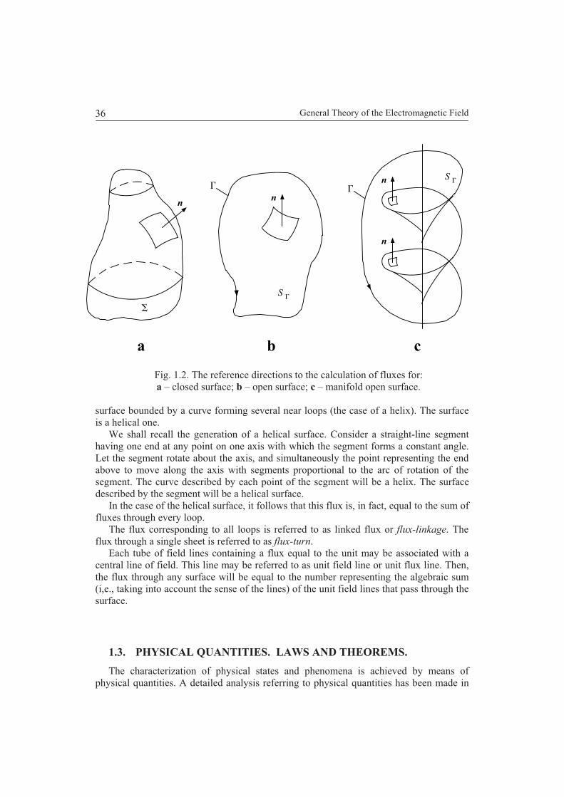
General Theory of the Electromagnetic Field36
Fig. 1.2. The reference directions to the calculation of fluxes for:a – closed surface; b – open surface; c – manifold open surface.
surface bounded by a curve forming several near loops (the case of a helix). The surfaceis a helical one.
We shall recall the generation of a helical surface. Consider a straight-line segmenthaving one end at any point on one axis with which the segment forms a constant angle.Let the segment rotate about the axis, and simultaneously the point representing the endabove to move along the axis with segments proportional to the arc of rotation of thesegment. The curve described by each point of the segment will be a helix. The surfacedescribed by the segment will be a helical surface.
In the case of the helical surface, it follows that this flux is, in fact, equal to the sum offluxes through every loop.
The flux corresponding to all loops is referred to as linked flux or flux-linkage. Theflux through a single sheet is referred to as flux-turn.
Each tube of field lines containing a flux equal to the unit may be associated with acentral line of field. This line may be referred to as unit field line or unit flux line. Then,the flux through any surface will be equal to the number representing the algebraic sum(i,e., taking into account the sense of the lines) of the unit field lines that pass through thesurface.
1.3. PHYSICAL QUANTITIES. LAWS AND THEOREMS.
The characterization of physical states and phenomena is achieved by means ofphysical quantities. A detailed analysis referring to physical quantities has been made in
nn
S
n
n
a b c
S

Generalities on the Theory of the Electromagnetic Field and on the Structure of Substance 37
several works [1], [8], [11], [21], [22]. Further on, some principal aspects will beexplained.
A kind of a physical quantity (in French, espèce de grandeurs physiques) is a class ofphysical properties susceptible of quantitative determination. For defining the kind of aphysical quantity, it is necessary to know the measuring procedure and the unit ofmeasure. The choice of the unit of measure is arbitrary. As examples, the following threekinds of quantities utilized in electromagnetism will be given: Electric charge, electricfield strength, magnetic field strength.
A kind of physical quantity characterizes a common property of the elements (objects)of a set of physical objects. To identify a common property of a set of physical objects, itis necessary that a relation of order should exist between these objects.
A measure procedure is a repeatable experimental operation, by which, to eachphysical quantity it is possible to associate a mathematical quantity called value ormagnitude in respect to a physical quantity termed unit.
According to the manner of introducing, the kinds of physical quantities can bedivided into the following ones: Kinds of primitive quantities and kinds of secondary(derived) quantities (in French, espèces de grandeurs primitives et espèces de grandeurssecondaires ou dérivées), also termed primitive and secondary (derived) quantities,respectively (in French, grandeurs primitives et, respectivement, grandeurs secondairesou dérivées). The kinds of secondary (derived) quantities can be defined by means ofother ones supposed as being known, hence introduced previously. The kinds of primitivequantities have to be introduced directly, by experimental way, and described by themeasurement procedure, because they can no more be defined by means of quantitiesintroduced previously.
In electromagnetism, apart from the primitive quantities of mechanics (length, time,mass, force), a series of new primitive quantities is necessary for characterizing from anelectromagnetic point of view the state of bodies and of the electromagnetic field.
A system of units contains fundamental and derived units (in French, unitésfondamentales ou de base et unités dérivées). The fundamental units have to bedetermined directly, experimentally (e.g., the metre). The derived units are derived byusing the fundamental units (e.g., the square metre). The fundamental units must not bethose of the primitive quantities, but those of the quantities that frequently appear inpractice.
The laws express relations that are essentially necessary and repeatable betweenphenomena. In physics, laws are called the relations that express the most generalknowledge on the phenomena of a research domain. They reflect the objective properties(of phenomena) that cannot be deduced by logical analysis (in the framework of therespective research field) from more general relations. The laws are established by thegeneralization of a great number of experimental results. In the theory of theelectromagnetic field, there are general laws and material laws also called constitutive
laws. The material laws differ from the general ones by the fact that they contain in theirexpression quantities specific to various materials, called material quantities.
The relations that can be deduced by logical analysis from other more general ones,and finally from laws, are called theorems.
It is useful to mention that there are relations that, at the time at which they wereestablished, had law character but subsequently, after the progress of science, moregeneral relations were discovered and the first ones could be derived or have represented
General Theory of the Electromagnetic Field38
particular cases. Therefore, many relations that have a theorem character are called, byhistorical reason, laws. Further, for more clarity, when necessary, each denomination willbe mentioned.
The examination of various quantities may be made in two ways, as the structure ofbodies is taken into consideration. Consequently, two manners of studying quantities andphenomena naturally appear: The microscopic manner of the study and the macroscopicone. Correspondingly, there are a microscopic theory of the electromagnetic field and amacroscopic theory of the electromagnetic field.
1.4. MANNERS OF STUDYING THE THEORY OFTHE ELECTROMAGNETIC FIELD
1.4.1. The Macroscopic Study of the Electromagnetic Field
The character of the macroscopic study (from the Ancient Greek; µ (makros)means long and (skopeo) means look at or examine) results from the fact that, inthe framework of the study, the atomic structure of bodies is not taken into consideration;it is assumed that the substance is continuously distributed throughout the whole space. Inthe case of macroscopic study, all relations are obtained by an analysis of the mode inwhich the phenomena manifest themselves at the scale of the human senses.
1.4.2. The Microscopic Study of the Electromagnetic Field
The character of the microscopic study (from the Ancient Greek; µ (mikros)means small and (skopeo) means examine) results from the fact that, in theframework of the study, the atomic discontinuous structure is taken into account.
1.4.3. Generalities Concerning the Microscopic Study ofthe Electromagnetic Field
The microscopic study of the electromagnetic fields takes into account the atomicdiscontinuous structure of bodies.
It is recalled that all bodies are constituted of atoms, and an atom of each body iscomposed of relatively light bodies called electrons that have negative charge, and of arelatively heavy nucleus. The nucleus is essentially constituted of protons, particles thathave a positive electric charge, and neutrons, particles that have no electric charge.
The electron is the smallest material particle with an indivisible negative charge. The
electric charge of an electron is 1910602.1e C, and its mass is
kg109108.0 30em .The proton is a particle with a positive electric charge equal in absolute value to that
of electron, and its mass is kg10672.1 27pm , hence approximately 1836 times
greater than the mass of electron. The neutron is a particle with zero electric charge, butwith the mass approximately equal to that of the proton.
Generalities on the Theory of the Electromagnetic Field and on the Structure of Substance
39
The substance is constituted of molecules that are formed of atoms. According to the Rutherford-Bohr-Sommerfeld atomic model, the substance presents itself in the form of planetary systems, each atom consisting of a nucleus with positive electric charge and of one or more electrons that turn about nucleus around closed orbits.
Concerning the form of a nucleus and of an electron, the simplest proposal is to consider them as being of spherical form. However, this supposition is not satisfactory and it is necessary to use the Quantum Mechanics. Also, there are possibilities of using models that permit to obtain results close to the various ones obtained experimentally [20, p. 64].
The dimensions of nucleus and electrons, in the framework of the simple physical model above, are so small, that in many phenomena, the atomic nuclei and the electrons can be considered of negligible dimensions. Hence, they can be considered as material points or point-like bodies with electric charge and mass. The study of the nucleus structure does not enter into the frame of the present work, and belongs to the domain of Nuclear Physics.
It is useful to be mentioned that, generally, one of the aims of Physics is the determination of the number, repartition and character of the particles charged with electricity which characterize the nature of bodies. Let us give the following example: The derivation of the laws of chemical and physical phenomena, by the aid of interaction laws of particles with electric charge.
The single important exception is represented by the phenomena in which an important function is represented by forces of mechanical nature (gravitation forces, elastic forces, capillary forces, friction forces, etc.) and nuclear forces, because only these forces cannot be reduced to the action of electric charges.
The characterization of the local state of the electromagnetic field in the macroscopic theory may be done by the help of local state quantities of the field: The electric field strength, the electric displacement (electric induction), the magnetic field strength, and the magnetic induction that will be further studied.
1.4.4. Macroscopic Average (Mean) Values
The macroscopic properties have to be described by means of macroscopic quantities. Macroscopic quantities are the quantities obtained by determining the average (mean) values of microscopic quantities for space domains and time intervals that are physically infinitesimal quantities (physically infinitesimal is in French, infiniment petit au sens physique [3, p. 408]). These mean values are called macroscopic average (mean) values.
By a physical infinitesimal domain of space (also called of volume) we understand a domain small enough, from a macroscopic point of view for, within it, the macroscopic quantities show a negligible variation with distance, and at the same time, great enough, from a microscopic point of view. The last condition means that the domain must contain a very great number of particles, i.e., molecules, atoms and elementary particles.
By a physical infinitesimal interval of time we understand a time interval small enough, from a macroscopic point of view for, within it, the macroscopic time-dependent quantities show a negligible variation with time, and at the same time great enough, from a microscopic point of view. The last condition means that the time interval must have the duration much greater than the duration of processes occurring at microscopic scale, i.e., molecular or atomic scale.
General Theory of the Electromagnetic Field40
The value of a physically infinitesimal volume depends on the nature of the substance
and can be considered of about 35 cm)10( . It can also be mentioned that the processesoccurring at microscopic scale (e.g., the variation of the electric field strength) aredepending on the period of the orbital motion of electrons [18, p. 50]. This period is of
about 1610 s. In fact, infinitesimal means infinitely small.
1.4.5. Manner of Studying Adopted in the Present Work
In the engineering practice, the study of phenomena at macroscopic scale is of aparticular interest, however, in many cases, it is necessary to know the phenomena at themicroscopic scale, as is the case of devices with semiconductor elements, elements ofintegrated circuits, devices with discharge in air, etc. Taking into account the physicalmodel, often relatively simple in the microscopic study, the following procedure will beused: Firstly, the various quantities and phenomena at microscopic scale will be studied,then, by calculating the average (mean) values, the phenomena at macroscopic scale willbe considered.
As starting point, the expression of the Coulomb force acting between two materialpoints with electric charge will be taken into account.
Considering material points with electric charge, in motion with respect to varioussystems of reference (i.e., reference frames), and taking into account the transformationrelations of the components of a force from the Special Theory of Relativity, the generalrelations of the Theory of the electromagnetic field can be obtained.
It is often stated that the observation of relativistic effects requires great velocities ofmoving bodies and measurements of high precision. However, in Electromagnetism,relativistic effects are encountered even in the case of small velocities compared to thevelocity of light. The component of the force referred to as being of magnetic nature andwhich acts upon a moving material point with electric charge, is a relativistic component.It represents a supplementary confirmation of the importance presented by the theory ofrelativity.
The study of phenomena encountered in electromagnetism at microscopic scalerequires the Quantum Mechanics. It is to be noted that by certain improvements of themodels of various particles, the same results can be obtained for certain cases withoututilizing the Quantum Mechanics [20].
1.4.6. Laws of the Theory of Electric and Magnetic Phenomena
From the explanation concerning the laws, it results that they can be grouped(classified) as follows. The macroscopic theory of electric and magnetic phenomena isconsidered to have twelve important laws, nine of them being general laws and three ofthem material laws.
The general laws are the following:1. The law of electromagnetic induction.2. The law of magnetic circuit (the magnetic circuital law).3. The law of electric flux (the Gauss law).4. The law of magnetic flux (the law of flux conservation).

Generalities on the Theory of the Electromagnetic Field and on the Structure of Substance 41
5. The law of the relationship between electric displacement (electric induction),electric field strength and electric polarization.
6. The law of the relationship between magnetic induction, magnetic field strength,and magnetization.
7. The law of conservation of free (true) electric charge.8. The law of the energy transformation in a body carrying conduction electric
current.9. Law of electrolysis.
The most important material laws are the following:1. The law of temporary electric polarization.2. The law of temporary magnetization.3. The law of electric conduction.To the general laws, the law of ponderomotive action upon a charged particle at rest
can be added, and is referred to as law of ponderomotive action. However, it is includedin the definition of the electric field strength.
The law of electrolysis will not be examined in this work. An explanation of this lawcan be found in works containing sections devoted to Electrochemistry [23], [48], [49].
The material laws exist only in the macroscopic theory. The material laws can bededuced from microscopic general laws under certain assumptions.
Four types of fundamental quantities macroscopically characterize the electromagneticstate of bodies: Electric charge q, electric moment p , density of the conduction electriccurrent J , magnetic moment m .
The state of the electromagnetic field is macroscopically characterized by thefollowing types of quantities: Electric field strength E , electric displacement (electricinduction) D , magnetic field strength H , magnetic induction (magnetic flux density)B . These kinds of state quantities are introduced by the help of two kinds of fundamentalquantities: Electric field strength in vacuo E and magnetic induction in vacuo B . Theelectromagnetic state of bodies and of the electromagnetic field is microscopicallycharacterized by three kinds of fundamental quantities: Electric charge q , electric fieldstrength E , magnetic induction B .
The microscopic theory of electric and magnetic phenomena has five general laws:1. The law of electromagnetic induction.2. The law of magnetic circuit or magnetic circuital law.3. The electric flux law (Gauss law).4. The magnetic flux law (the magnetic flux conservation law).5. The law of ponderomotive action upon a moving electrically charged particle.

General Theory of the Electromagnetic Field42
1.5. GENERAL CONSIDERATIONS ON THE STRUCTURE OFCONDUCTORS AND DIELECTRICS
1.5.1. Electrically Conductive Materials
The electrically conductive (conducting) materials are substances that, in normalconditions of use, have good electricity conducting properties (therefore they permit therapid moving of particles charged with electricity within their interior).
The objects, pieces built of electrically conductive materials are called electric
conductors or simply conductors.There are two kinds of conductors:a. Conductors of the first kind, in which, no chemical reaction occurs when they are
carrying an electric current. This is the case of metals, metal alloys, carbon,semiconductors.
b. Conductors of the second kind, in which, chemical reactions occur when they arecarrying an electric current. This is the case of electrolytes.
In metals, a part of the electrons that belong to the structure of an atom leaves theatom (hence they are delocalized), for this reason, these electrons are referred to as free
electrons. These free electrons can move to large distances inside the conductor, ensuringthe displacement of electric charges.
The conductors of the second kind contain in their structure ions. Every ion has anexceeding electric charge with respect to the neutral state. The ions can move to relativelylarge distances inside the conductor, ensuring the displacement of electric charges.
The earth also shows conducting properties. Therefore, in conductors there areparticles that can displace themselves, carrying electric charges. They can be called free
charged particles or free electric charges.The most utilized materials in construction of installation and electrical equipment are
copper and aluminium because of their great conductivity. Also, alloys of copper withother elements are used. The conductors are produced in form of wire or strip. The cross-section of a wire may be circular or rectangular.
The conductors are insulated for achieving various circuits and for avoiding defectionsor accidents. When an electric current flows through a conductor, this conductor heatsand it is necessary to take into account that the utilization temperature is limited. For anon-insulated conductor, the limitation is determined by the mechanical strength of theequipment at high temperature. That is why, temperature of 200 – 300 ºC may not besurpassed.
For insulated conductors, the limitation is determined by the utilisation of thetemperature of the insulation.
For achieving contacts, the following materials are utilized: Copper, silver, tungsten(wolfram), in pure form or alloys with other elements or in the form of sintered powders.
1.5.2. Dielectrics
Dielectrics are substances that in normal conditions in which they are utilized, are badelectricity conductors (i.e., they permit with difficulty the moving of electric charges),

Generalities on the Theory of the Electromagnetic Field and on the Structure of Substance 43
because in general they do not contain free microscopic particles charged with electricity,which could displace themselves to relatively large distances.
Insulating materials are adopted from dielectrics. Any piece called insulator isachieved of an insulating material.
Dielectrics are solid, liquid or gaseous substances formed of systems of electriccharges, namely neutral small domains (hence, the sum of electric charges of the interiorof each domain is zero).
Dielectrics may be divided, from the point of view of the distribution of electriccharges, into two fundamental groups: Polar and non-polar.
Dielectrics with polar and non-polar molecules have both positive and negativeelectric charges, equal in absolute value. The centre of mass of the particles with positivecharge and with negative charge, respectively, may coincide (first case) or not (secondcase) in space, depending on the type of molecule, i.e., of the substance. In the first casethe molecule has an electric moment only in the presence of an external electric field. Inthis case, it is a non-polar dielectric. In the second case, the molecule has an electricmoment even in the absence of an external electric field. In this case, it is a polardielectric.
Examples of non-polar dielectrics: Mono-atomic inert gases (He, Ne, Ar, Kr, Xe),diatomic gases ( 2H , 2N , 2Cl ), hydrocarbons and hydrocarbon composition (petroleum
oils, polyethylene, polystyrene), carbon dioxide ( 2CO ), methane, benzene 66HC ,NaCl (ionic crystals).
Examples of polar dielectrics: Hydrocarbon when some atoms or groups of atomssubstitute hydrogen atoms like nitrobenzene ( 256 NOHC ), methyl chloride ClCH3 ,water (a typical polar substance) having the electric moment of a molecule
mC101.6 30p . In the above cases, hqp d ; C10 19dq ; m10 10h .
In the case of dielectrics, the particles charged with electricity cannot leave the systemof particles, namely atoms, molecules, ions, to which they belong. Always, the sum ofelectric charge is zero for the system to which they belong, that is why these particles arecalled bound particles, and the corresponding electric charges – bound electric charges.Dielectrics can be charged by free electric charges, brought from outside.
Dielectrics may be divided from the point of view of the distribution of electriccharges and types of molecules into the three following groups:
a. Dielectrics constituted by particles grouped in neutral molecules. This is the casefor all dielectrics in gaseous or liquid form and for a part of those in solid form.
b. Dielectrics that besides the particles grouped in neutral molecules also containions, the last being fixed in certain equilibrium positions, for instance at the nodesof the crystalline lattice of the body. The ionic crystalline lattices are composed ofelementary domains, and each domain is charged with positive and negativecharges equal in absolute value, so that the domains globally appear as neutral.This is the case especially for crystalline dielectrics like quartz, mica, anhydrousoxide of aluminium, rutile ( 2TiO ).
c. Dielectrics that besides neutral molecules also contain molecules charged withpositive and negative charges equal in absolute value, called dipolar molecules.This is the case of organic materials (cellulose, heat-convertible materials), glass,glass materials, certain crystalline dielectrics (ice).

General Theory of the Electromagnetic Field44
Electrically insulating materials are used for the insulation of the parts of theinstallations that are at an electric potential difference (voltage), carry an electric currentor are used in various electrical devices. The insulation of conductors is necessary, asshown, in the achievement of installations, and for avoiding damages and accidents.
The electrically insulating materials can be classified according to the allowableoperation temperatures. These values have been established, taking into account theoperating conditions, for obtaining satisfactory service duration.
The electrically insulating materials are in gaseous liquid or solid form:1. Gaseous form: Gaseous dielectrics.2. Liquid form: Petroleum oils, synthetic liquids like silicon liquids.3. Solid form: Polymers composing thermoplastic materials, cellulose, silk,thermosetting materials (thermohardening materials), varnishes, compounds, plasticcompounds of binder (organic polymer capable of deformation) and powder like filler,fibrous or sheets of cotton, mica, paper, fibrous materials, glasses, ceramic materials.
1.6. ELECTRIC CHARGE. ELECTRIC FIELD STRENGTH IN VACUO
1.6.1. Electrification State. Electric Field.
First, the state of electrification of bodies will be considered. We shall consider a setcomposed of a piece of polished glass and a piece of resin, with no mechanical actionsbetween them. Let the piece of glass and the piece of resin to be rubbed together, and thenseparated from each other. The two pieces will attract each other. We shall consider asecond set also composed of a piece of polished glass and a piece of resin. The pieces ofthe second set will be subjected to the same operation as the pieces of the first set. We canobserve that between the pieces above, ponderomotive actions are exerted as follows:
1. Each piece of glass attracts each piece of resin.2. Each piece of resin attracts each piece of glass.3. Each piece of glass repels each other piece of glass.4. Each piece of resin repels each other piece of resin.5. Each piece of glass as well as each piece of resin does not exert a force on a set
composed of a piece of glass and a piece of resin that have not been separated.Therefore, ponderomotive actions that did not exist previously appear. In this
situation, the system formed by certain or by all bodies above is considered to beelectrified, and each of these bodies is considered to be an electrified body.
This type of electrification is called electrification by friction. Electrified state ofbodies is called any state in which these bodies exert ponderomotive actions of electricalnature upon other bodies, i.e., actions of the same nature with the one exerted by thebodies electrified by friction.
If a body has the same behaviour as the piece of glass above, the body is considered asvitreously electrified. If a body has the same behaviour as the pieces of resin above, thebody is considered to be resinously electrified. Conventionally, the vitreouslyelectrification was called positive electrification and the resinously electrification wascalled negative electrification.

Generalities on the Theory of the Electromagnetic Field and on the Structure of Substance 45
The positive electrification of a piece of glass can also be obtained by friction with apiece of cloth or texture. It is worth noting that the non-polished glass will not beelectrified. Details are given in the work [12, tome III, p. 362].
The electrification by friction appears on the contact surfaces of two bodies, at leastone of them being a dielectric (insulating material), as a result of friction when the twobodies are in relative motion. In the case of non-metallic bodies, electric charges, i.e.,electrons, are delivered on a superficial film (pellicle) as a result of friction abrasion.
From a microscopic point of view, the electrification state of a body means that it is inthe situation of having an excess or lack of electrons.
It was experimentally established that there is a great number of possibilities forelectrifying a system of bodies: By contact (temporary or permanent) with electrifiedbodies, by deformation, by thermal action, by irradiation.
The electrification can be communicated from an electrified body to a non-electrifiedone, by contact or by influence. It is useful to mention that the electrification by influencemeans in fact a modification of the repartition of the electric charge, i.e., of the electronsin a conducting body under the influence of the charge of another body.
According to the transmission duration of the electrification state, the materials can bedivided into three categories:
a. Electric conductors or simpler conductors that transmit the electrification state in
a very short time, of the order of 1210 s, thus nearly instantaneously. The bodiesmade of such material are also called conductors.
b. Electric insulators or simpler insulators that transmit the electrification state in avery long time of the order of hours or days.
c. Semiconductors that transmit the electrification state in an intermediary time, ofthe order of second fractions.
The ponderomotive actions that are exerted on the bodies situated in theneighbourhood of electrified bodies make evident the existence of the electrified system,in the space surrounding the electrified field.
In accordance with the general definition of Section 1.1, electric field is called thephysical system that exists in the space regions in which ponderomotive actions (forcesand torques) of electric nature can act on bodies.
The interactions between electrified bodies are produced by means of electric fieldproduced by the electrified bodies. This fact was established by Faraday and Maxwell.The preceding statement represents, in fact, a general rule accepted in Physics and calledprinciple of continuity: Two bodies can interact only by means of an intermediarymedium (i.e., throughout the intermediary medium between the bodies). Hence all lawshave to be expressed in a differential form concerning points infinitely close to eachother.
1.6.2. True Electric Charge (Free Electric Charge)
The mechanical and thermal quantities do not suffice for the study of theelectrification state and of the electric field. Therefore, it is necessary to introduceexperimentally new physical quantities that will be primitive (fundamental) quantities inthe framework of the theory of the electromagnetic field.

General Theory of the Electromagnetic Field46
From Sub-section 1.6.1, it follows that there are two kinds of electrification state:positive and negative. The electrification state of an electrified body, namely theelectrified piece of resin of Sub-section 1.6.1, will be considered as reference state. Thiselectrification state is, as shown, negative.
To introduce the physical quantity called true (free) electric charge; the followingmeasuring procedure can be used. All bodies under consideration in this procedure areconsidered to be very small, i.e., their dimensions are negligible compared with thedistances between them.
Several small bodies in identical electrification state will be considered. All thesebodies will be termed reference bodies.
As shown in Sub-section 1.6.1, no ponderomotive force acts on the system composedof a piece of glass and a piece of resin if the system is under the action of an electrifiedbody, hence, if it is in an electric field. This system is called neutral system. Theoperation of bringing together two or several electrified bodies, so that the resultingsystem will not be subjected to a ponderomotive force, in an electric field, is calledneutralization. Therefore, the true electric charge of any body is proportional to thenumber of reference bodies necessary for the neutralization of the given body.
The unit (of measure) of the true (free) electric charge may be adopted by conventionthat of one reference body, [8, Vol. I], [23, Vol. I, p. 46].
The proportionality constant is the negative unity. In this case, the true (free) electriccharge of the given body is equal to the number of reference bodies and with oppositesign with respect to the last ones.
Hence, the electric charge has been introduced in a non-correlative way, i.e.,regardless of the electric field strength. At the same time, it follows that the electriccharge introduced in this way is independent of the reference frame (reference system) orof the velocity. The previous terms true and free can be considered synonyms, howevercertain authors are using the term true in the macroscopic approach and free in themicroscopic approach.
It is to be noted that the electric charge of a moving body does not vary like the massof the body with the velocity. This fact has been established experimentally observingthat, in the case in which the number of protons of one atom nucleus is equal to thenumber of electrons turning about the nucleus, the neutral state of atoms is maintained,although the velocity of electrons and nuclei, respectively, are different. For this reason,hydrogen atoms or molecules are not deflected by an electric field. This fact is referred toas constant charge principle [18, p. 17].
It follows that the true electric charge is a property of bodies, characterized by a scalarquantity proportional to the number of electrons that are not neutralized by the positivecharge of the nuclei of the constitution of bodies. The electric charge of a body isnegative if it is an excess of electrons and positive if it is a lack of electrons. From themicroscopic point of view, the electric charge is distributed among the microscopicparticles of the respective body. Each microscopic particle of a certain type has alwaysthe same electric charge. From a microscopic point of view, the electric charge isdistributed discontinuously in space.
From a macroscopic point of view, it is assumed that the true (free) electric charge,like the substance, is distributed continuously within the whole domain occupied by theconsidered body. Therefore, the macroscopic representation is an idealized one but
Generalities on the Theory of the Electromagnetic Field and on the Structure of Substance 47
permits, in many applications, to simplify the calculations and ensures a very goodaccuracy.
The true electric charge and electric field strength in vacuo are primitive(fundamental) quantities in the framework of the microscopic theory, as well as in theframework of the macroscopic theory of the electromagnetic field. The particles withelectric charge, like electrons and ions, which can move carrying electric charge, arecalled electric charge carriers.
In many cases, it is necessary to consider small bodies with electric charge. Since theelectric charge, as mentioned above, is a property of bodies, the more exact wording isone of the following: A small body charged with the electric charge q; a point-like charge
q; a point charge q.The electric charge of a body is also denoted by q and can be termed electric charge
or quantity of electricity.The unit (of measure) of electric charge in the SI system of units is the coulomb
(symbol C); its definition will be examined in Section 1.15.
1.6.3. Density of Electric Charge
The local state of electrification is characterized by the volume distribution of theelectric charge. The volume density of the electric charge at any point of the body isdefined as the ratio of the following quantities: The electric charge, denoted q ,contained within the domain bounded by a small closed surface including that point,and the volume v bounded by the above surface, which is a physically infinitesimalvolume. As a macroscopic quantity, the electric charge may be considered continuouslydistributed in the space occupied by any body. In this case, the macroscopic volume
density of the electric charge may be introduced in the form:
.d
dlim
0 v
q
v
q
vv (1.7)
The electric charges may sometimes be distributed in a very thin layer over certainsurfaces. Then, the idealized macroscopic case will be considered. In this case, theelectric charge is distributed on these surfaces, considered as discontinuity surfaces.Therefore, the macroscopic surface density of the electric charge may be introduced inthe form:
.d
dlim
0 S
q
S
q SS
Ss (1.8)
The electric charges may sometimes be distributed very non-uniformly and may beconcentrated about certain lines. Also, the idealized macroscopic case will be considered.In this case, the electric charge is distributed along these lines, considered as discontinuitylines. The macroscopic line density of the electric charge may be introduced in the form:
.d
dlim
0 l
q
l
q ll
ll (1.9)

General Theory of the Electromagnetic Field48
The domains v , S , l above utilized, in the denominators of relations (1.7), (1.8),(1.9), were firstly considered physically infinitesimal space quantities, but when assuminga continuous distribution of the electric charge they are assumed as tending to zero.
In many cases, it is necessary to calculate the average value with respect to space andtime that may be denoted by the suffixes v and t respectively.
The quantity obtained by calculating the average value of the microscopic values maybe designated by writing that microscopic quantity within the following angle brackets
suffix and the subscript of the second sign (here written suffix) indicates the quantity
with respect to which the average value has to be calculated. If the average value has tobe calculated with respect to two or more variables, then, the microscopic quantity will bewritten between two or more pairs of signs, as above, with the corresponding subscripts.If only a pair of signs is used and no suffix is written, it is considered that the averageconcerns both, space and time. More details and examples will be given in Sub-section1.6.6.
The macroscopic electric charge densities above defined are the average values (mean
values) and can be expressed in terms of the microscopic electric charge density:
.;;tlfreemicrol
tsfreemicrostvfreemicro lsvv (1.10 a, b, c)
The electric charges are also referred to as quantities of electricity, in the cases ofvolume, surface or line distribution, respectively, and are given by the followingrelations:
.d;d;d
qqq C
ll
S
sS
V
vv lqSqvq(1.11 a, b, c)
1.6.4. Conservation of the Free (True) Electric Charges
The total electric charge of an isolated system of bodies, i.e., situated in vacuo andsurrounded by insulators, is constant. Certain explanation will be added.
At a given moment, it is possible that a certain electric charge appears in one region(zone) of the domain, where before no electric charge existed. However, at the same time,a certain electric charge disappears in another region of the domain. In such cases, thetotal electric charge is conserved, namely when in one region of the domain a charge q
appears, a charge q simultaneously appears in another region, because the number ofcharge carriers of the system of bodies remains the same.
1.6.5. The Electric Field Strength in Vacuo
Any reference frame will be considered. Let F be the force exerted in vacuo (i.e.,empty space) on a small body with a small free electric charge q at rest in the referenceframe in which the force is measured. The charge has been assumed to be small enough,in order of not disturbing the distribution of the other electric charges.

Generalities on the Theory of the Electromagnetic Field and on the Structure of Substance 49
It can be experimentally established that the ratio between the two quantities does notdepend on the electrification state of the above body, but depends only on the localelectric state of the electric field. Therefore, the following relation can be written:
,q
FE (1.12)
where the quantity E is independent of the true electric charge q . The quantity E iscalled the electric field strength in vacuo. Hence, the electric field strength at a point isdefined in a certain reference frame, as the ratio of the force acting upon a point-likeelectric charge at rest at the considered point (with respect to the adopted referenceframe), to the value of the electric charge.
In order to explore an electric field and thus find its strength at any point, a smallbody, satisfying the conditions below can be used. The conditions to be fulfilled by thebody are the following:
a. Small enough dimensions, for permitting the measurement of the forces in verysmall regions of the field.
b. Small enough electric charge in order of not disturbing the electric state of thedomain.
c. Build of conducting material, electrically very well insulated for permitting aneasy transfer of electric charge.
The small body fulfilling the conditions above is referred to as proof body or test body
(in French, corps d’épreuve). The test body will permit to determine the value of themacroscopic field strength of the electric field at a point in empty space or in a gaseousmedium, according to the relation:
,lim0 qq
FE (1.13)
where F is the force acting upon the test body and q is the electric charge of the body asmentioned below. In the case in which a continuous distribution of the electric charge isassumed, the value of q is supposed as tending to zero, actually, to a value small enough,different from zero.
Consequently, the following relation can be used in the case of point-like charges:
.EF q (1.14)
Formula (1.14) expresses a general relationship referred to as expression or law of the
ponderomotive action upon one point-like electric charge at rest in the reference frame inwhich the force is expressed. It can also be considered as a relation used for defining thequantity E .
In accordance with relation (1.14), and with the definition of the lines of field of Sub-section 1.2.1, it follows that a line of field that passes through any point is just thetrajectory of a particle with a very small electric charge (for not disturbing the state of thefield) and with a very small velocity (otherwise the relation is no more valid), whichpasses through the considered point. The direction of the line of field is the directionalong which a particle, positively charged, is moving.

General Theory of the Electromagnetic Field50
1.6.6. The Macroscopic Electric Field Strength
The macroscopic electric field strength at a point is obtained by calculating theaverage value of the microscopic electric field strength. According to the definition, themacroscopic electric field strength E at a certain point rN , at the moment t, in anyreference frame will be calculated.
For this purpose, a physically infinitesimal volume v having at its centre theconsidered point, will be chosen, and a physically infinitesimal time interval 0t , will be
chosen so that the moment t will be at its middle. We shall denote by t,micro rE themicroscopic electric field strength at a point within the volume element v at a moment
2,
200 t
tt
tt . The macroscopic electric field strength will be obtained by
calculating the average value of the microscopic field strength by the relation:
v
t
t
tvtttv
t .dd,1
, 00micro
2
2
0tvmicromacro
0
00
rEErEE (1.15 a)
In solids, a physically infinitesimal volume must be much greater than the volumeattributed to an atom assumed to be bounded by a sphere having a radius of about
cm10 8 , but small enough at macroscopic scale. This small volume may be assumed to
be a cube, or a sphere having a radius of about cm1010 54 . In the mentioned small
volume, the number of atoms is of approximately 910 . Another example, a cubic
centimetre of copper contains approximately 2310 atoms and 22105.8 free electrons.The physically infinitesimal time interval must be much greater than the period of
time variation of atomic phenomena, namely the period of the orbital motion of electrons
is of about s1610 , but small enough at macroscopic scale, therefore it may be assumed
of s1312 1010 .If a three-orthogonal rectilinear system of co-ordinates is used, the volume v will be
that of a right parallelepiped having the sides 000 ,, zyx , and it follows:
2
2
0000000micro
2
2
2
2
2
2
00000
0
0
0
0
0
0
0
0
.ddd,,,
d1
,
x
x
z
z
y
y
t
t
zyxttzzyyxx
ttzyx
t
E
rE
(1.15 b)

Generalities on the Theory of the Electromagnetic Field and on the Structure of Substance 51
From the last relation, it results that [2], [3], [21]:
,,,tv
micro tx
tx
rErE (1.15 c)
and
,,,tv
micro tt
tt
rErE (1.15 d)
where the indices v and t refer to the averages with respect to volume (space) and timerespectively.
The last two relations are useful in certain linear relations containing derivatives thathave been obtained for microscopic quantities; the same relations will be valid formacroscopic quantities.
Within a physically infinitesimal volume and a physically infinitesimal time interval,the distribution of charges may be assumed as uniform. The average value of the sum ofthe forces acting upon the particles charged with electricity and belonging to theconsidered small volume will contain the following two terms. The first term will be theproduct of the average value of the electric charge q of the volume and the average valueof the electric field strength. The second term will represent the average value of theproduct:
macro
macro
macromicromicromicromacromicro
;
;
EE
EEE
vv
vvv
(1.16)
that are not taken into consideration in the macroscopic studies.It is interesting to remark that the microscopic field strength can vary very much from
one point to another. This aspect will be highlighted by examining the electric field ofelectrons. A simple model of an electron is a sphere charged with electricity. The electroncharge may be assumed as distributed over the surface or within the volume of the sphere.The radius of the sphere attributed to the volume occupied by the electron is of about
cm108.2 13 . The density of the electric charge of this model is very great. The electricfield strength in the electron vicinity is very great and changes its sign at the extremitiesof each diameter of the sphere attributed to the electron, thus it shows considerable
variations at distances of the order of cm10 13 .The average value of other physical quantities can be calculated in the same manner as
above.Further on, if no special mention is made concerning a quantity, that quantity will be
considered as a macroscopic one.

General Theory of the Electromagnetic Field52
1.7. ELECTRIC FIELD STRENGTH IN THE LARGE SENSE
If at a point of any medium, there is a particle with the electric charge q, very small sothat it has a negligible effect on the resultant electric field, and at rest in the referenceframe, the electric field strength at that point is given by the following relation (Fig. 1.3):
,
,
el-nonel FFF
FE
ql
(1.17)
where F is the force acting on that particle, in the same reference frame. The component
elF is of electric nature and the component el-nonF is of non-electric nature. The force F
denotes the total force regardless of the nature of its components.The particle with the electric charge q is assumed as belonging to the considered
medium; it is no more a test body.The macroscopic field strength at any point of a solid, a liquid or a gaseous medium,
in the framework of the macroscopic theory of the electromagnetic field, is a primitive(fundamental) quantity. For this reason, it has to be introduced experimentally, hencedirectly. This introduction can be done using cavities of certain forms and taking intoaccount the relations between the field quantities before and after having achieved thesecavities.
The subject has been widely analysed in literature [1], [5], [8], [12], [21].According to its nature, a field of vectors can have components of two types:a – Potential component pG , the curl of which is zero at any point of the space, but
the divergence of which may be different from zero.b – Solenoidal component rG , the curl of which is different from zero at least within
certain regions of the space, but the divergence of which is zero.
Fig. 1.3. Explanation concerning theelectric field strength in the large sense.
F Eq l=
O y
z
q
x
Generalities on the Theory of the Electromagnetic Field and on the Structure of Substance 53
This separation of components can also be used in the case of electric field. Accordingto the nature of the components of the force F , the electric field strength in the large
sense, lE , may have components of three types:
1º The Coulombian electric field strength, cE , which is produced by electric charges
according to the Coulomb law. This is a potential component, hence Vc gradE ,where the function V is the potential function.
2º The induced electric field strength (also termed rotational, curl, or solenoidal fieldstrength), rE , which is produced by the electromagnetic induction phenomenon.
3º The impressed electric field strength also termed extraneous electric field strength
[7, English edition, p. 12] (in French, champ électrique imprimé ou champ électromoteur[3, p. 135], in German, eingeprägte elektrische Feldstärke [22, p. 109]), iE , which is notproduced by electromagnetic causes, but by non-electromagnetic causes. Among thesecauses, the following ones can be mentioned:
a. Mechanical cause, for instance the acceleration of a metallic body that determinesforces which produce a displacement of electrons with respect to the positive ions of thecrystalline lattice of the metal.
b. Thermal or chemical phenomena determining forces which produce a displacementof electric charge carriers. To every force described above an electric field strengthcorresponds according to relation (1.17), and it is called impressed electric field strength.
Therefore, the expression of the electric field strength in the large sense is:
ircl EEEE (1.18)
or
,ncl EEE (1.18 a)
,rc EEE (1.18 b)
,il EEE (1.18 c)
where
irn EEE (1.19)
is referred to as the strength of the electromotive field or the strength of the non-Coulombian electric field, and
rc EEE (1.20)
represents the strength of the electric field in the restricted sense or simpler the strength
of the electric field.It can be added that the electric field strength is also referred to as electric field
intensity.The lines of the vector field E , i.e., lines of electric field strength, also called simply
electric field lines, are the lines at each point of which the vector E is tangent.

General Theory of the Electromagnetic Field54
1.8. LINE-INTEGRAL (CIRCULATION) OF THE ELECTRIC FIELDSTRENGTH ALONG AN ARC OF CURVE. ELECTRICPOTENTIAL DIFFERENCE. ELECTRIC TENSION, VOLTAGE.ELECTROMOTIVE FORCE.
Generally, in a field of vectors, the line-integral of a field vector round a curve or anarc of curve, like in the case of a work, is also called circulation along the respective way.In the case of an electric field, this circulation is referred to as electric tension also termedvoltage, in order to avoid any confusion with a mechanical meaning. This quantity is aderived one and will also be utilized in the study of the electric field.
A point-like electric charge that is moving with a very small velocity along any opencurve ABC in an electric field will be considered (Fig. 1.4). It is supposed that the chargeq is small enough so that it will not sensibly modify the state of the electric field.
The resultant force F , acting upon the considered particle, having one component ofelectric nature elF and another of non-electric nature el-nonF does the work:
.d
ABC
LW lF (1.21)
Utilizing expressions (1.18) and (1.21), it follows:
ABAB C
irc
C
lL qqW .dd lEEElE (1.21 a)
The ratio
ABC
lL
q
WlE d (1.22)
is independent of the electric charge of the particle that is moving along the curve ABC
and characterizes the work done when the point-like charge is moving along the curve.The velocity of the point-like charge is assumed small enough so that the force acting onit will be given by relation (1.17).
Fig. 1.4. Explanation to the calculation ofthe line-integral of the electric field
strength.
A
d l
F
q BCAB
Generalities on the Theory of the Electromagnetic Field and on the Structure of Substance 55
The line-integral of the electric field strength in the large sense, along the consideredcurve, is called electric tension in the large sense along the considered curve and is givenby the relation:
.d
AB
AB
C
llCu lE (1.23 a)
If instead of the electric field strength in the large sense lE , the electric field strengthin the restricted sense E is introduced in relation (1.23 a), the line-integral along theconsidered curve is also called electric tension and is given by the relation:
.d
AB
AB
C
Cu lE (1.23 b)
In accordance with relations (1.22) and (1.23 b), it follows:
.ABCL uqW (1.23 c)
If instead of the electric field strength in the large sense lE , the non-Coulombian
electric field strength nE is introduced in relation (1.23 a), the line-integral along theconsidered curve is also called electromotive tension or electromotive force and is givenby the relation:
.d
AB
AB
C
nCeu lE (1.24)
If the integrals (1.23 a) and (1.23 b) are considered around a closed curve , theobtained expressions is called electromotive force (e.m.f.) or electromotive tension in the
large sense and in the restricted sense, respectively; or each of them is simply calledelectromotive force (abbreviation e.m.f.). Therefore, the following relations:
,d lElleue (1.24 a)
,d lEeue (1.24 b)
are obtained, respectively.The electromotive force obtained by the line-integral of the electric field strength in
the large sense around a closed curve coincides with the integral of the non-Coulombiancomponent of the electric field strength along that closed curve. The reason is that theintegral of the Coulombian component of the electric field strength is zero.
If instead of the electric field strength in the large sense lE , the Coulombian electric
field strength cE is introduced in relation (1.23 a), the line-integral along the considered
curve ABC yields:
General Theory of the Electromagnetic Field56
ABBA
B
ACC
CC
C
c
uVVVVzz
Vy
y
Vx
x
V
zyxz
V
y
V
x
VV
ABAB
ABAB
AB
ddddd
ddddgradd kjikjillE
(1.24 c)
and is called electric tension, simply tension or voltage between the points A and B orpotential difference (p.d.) between the points A and B. This potential difference betweentwo points does not depend on the form of the curve ABC but only on the position of the
two points. If the curve ABC is closed, the integral (1.24 c) is zero.All the definitions given for electric tensions and electromotive forces refer to any
medium, regardless of its nature.The unit of electric tensions, potential difference and electromotive forces in the SI
system of units (which is a rationalized system) is the volt (symbol V) and is explained inSub-section 1.15.3.
1.9. POLARIZATION OF DIELECTRICS
1.9.1. The Polarization of Dielectrics Phenomenon. Polarization State ofDielectrics. Polarization Electric Charge (Bound Electric Charge).Electric Moment of a Neutral System of Electric Charges.
As shown in Sub-section 1.5.2, dielectrics consist of neutral systems (atoms, neutralmolecules, neutral domains) of electric charges. The electrically charged particles of eachsystem cannot move to relatively great distances, with respect to certain equilibriumpositions. For this reason, these charges are called bound electric charges.
Although they have this denomination, they are of the same nature as the free electriccharges. For each neutral system, the sum of all bound electric charges is zero. Therefore:
.01
bound
n
i
iq (1.25)
Under the action of an external electric field, the bound electrically charged particlesare not dislodged from their places (if the electric field strength is not too great), but theyare dislodged from their equilibrium into other neighbouring positions. Consequently, theelectric positive charges move in the direction of the electric field, and the negativeelectric charges move in the opposite direction.
Generalities on the Theory of the Electromagnetic Field and on the Structure of Substance
57
Therefore, the space distribution of the electric charges of the dielectric is modified. The new state of the dielectric is called electric polarization state. The respective phenomenon is termed electric polarization.
The metallic conductors are practically not polarizable. A neutral system of electric charges can be characterized by a vector quantity called
electric moment of the system. In any reference frame, let a neutral system be composed of n electrically charged particles that can be considered as point-like charges
( )niqi ,...,1, = , with the position vectors ( )nii ,...,1, =r having their origin at the same point of the reference frame (Fig. 1.5). If one point-like electric charge is moving within the system around a closed orbit (as the case of electrons can be), when considering the average value with time, the end (extremity) of the vector ir is considered as the action centre of the respective charge (i.e., the centre of the orbit).
The electric moment of a neutral system of point-like electric charges is:
,1 1
bound∑ ∑= =
==n
i
n
iiiis q prp (1.26)
with
∑=
=n
iiq
1bound .0 (1.26 a)
The relation (1.26) can serve to the characterization of a neutral system of electric charges, because the electric moment sp previously defined is independent of the choice of the reference frame. Indeed, if the origin of the reference frame is displaced from the point O to the point O’ (Fig. 1.5 a) by any vector a , then the electric moment of the neutral system in the new reference frame becomes:
( ) ∑∑∑ ∑=== =
−=−=′=′n
ii
n
iii
n
i
n
iiiiis qqqq
1bound
1bound
1 1boundbound .ararrp (1.26 b)
But
∑=
=n
iiq
1bound .0a (1.26 c)
It follows:
.1
bound s
n
iiis q prp ∑
=
==′ (1.26 d)
Remark. It is useful to mention that the above definition of the electric moment has not an arbitrary character. It implicitly occurs in the expression of the electric potential produced by a neutral system of point-like charges at a relatively distant point and it remains only to denote it, as done above.

General Theory of the Electromagnetic Field58
Fig. 1.5. Explanation concerning the electric moment of a neutral system of electriccharges: a – system with n charges; b – system with two charges (dipole).
The simplest neutral system of point-like electric charges is formed by two point-likeelectric charges equal in absolute value but of opposite signs q and q , like in Fig.1.5. This neutral system is called electric dipole or electric doublet, or shortly dipole ordoublet. A neutral system formed of several electric charges is called electric multipole ormultipole.
The electric moment of an electric dipole is (Fig. 1.5 b):
,212
2
11bound dddd
i
diid qqqqq hrrrrrp (1.27)
where the vector dh is always oriented as in Fig. 1.5. b, from the charge considered asnegative to the charge considered as positive.
1.9.2. The Macroscopic Electric Moment of a Polarized Body
The macroscopic electric moment of a polarized body can be obtained by performingthe sum of the electric moments sp of all the neutral systems forming the body andcalculating the average value over a physically infinitesimal time interval.
The calculation of the average value with respect to time is necessary because thecharges move round their trajectories and also because of their thermal agitation.
It results that the electric moment of a polarized dielectric body of volume DV is:
,
t
bound
t
i
V
i
V
s
DD
q rpp (1.28)
n boundqq
boundqi
d+
q d
O OO'
boundq
r n
r
r
r
1
r'
a
hd
2
1
iir
1
a b

Generalities on the Theory of the Electromagnetic Field and on the Structure of Substance 59
where the suffix t indicates that the calculation of the average value refers to time. Thesum is extended over all bound electric charges, electrons and atomic nuclei that arecontained in the volume DV of the dielectric body. In the case of a dielectric dipole,relation (1.28) yields:
.t
t
hhpp ddd
V
d qq
D
(1.28 a)
From a macroscopic point of view, because it is not possible to consider the structureof substance (electrons and nuclei); the electric moment of a body cannot be deduced asabove and for this reason it is not a secondary (derived) quantity. It follows that, in themacroscopic study, the electric moment of a body has to be introduced experimentally asa primitive (fundamental) quantity. This procedure can be achieved by considering theponderomotive actions exerted upon a small-polarized body, in an external electric field.
1.9.3. The Polarization Electric Charge. Density of the PolarizationElectric Charge.
As shown, dielectrics are constituted of neutral systems. Hence the total electriccharge due to the neutral systems inside the surface bounding the body is zero.
We shall consider (imagine) any macroscopic closed surface situated inside adielectric body. The sum of bound electric charges of the interior of the closed surface is called polarization electric charge or electric polarization charge of the interior of thatsurface and is denoted by pq . Therefore, the polarization electric charge is a
macroscopic charge. The manner of introducing this charge is analogous to that utilizedfor the free electric charge.
A dielectric is composed of numerous neutral systems. Hence, the neutral systems thatare entirely in the interior of the surface yield a total charge equal to zero. Since theclosed surface intersects several neutral systems of the dielectric, some electric chargesbelonging to the neutral systems the centres of which are inside the surface remainoutside this surface. It results that the total electric charge that remains inside the surfacemay be different from zero. Therefore, the total electric charge of the interior of theclosed surface is equal to the sum of the electric charges of the interior of the closedsurface that belong to the neutral systems intersected by the closed surface.
As a macroscopic quantity, the polarization electric charge may be consideredcontinuously distributed in the space occupied by the dielectric. In this case, a volume
density of the polarization electric charge may be introduced:
.d
dlim
0 v
q
v
q pp
vpv (1.29)
The neutral systems are not uniformly distributed, but they are more agglomerated incertain regions; hence, the volume density of the charge in these regions can have valuesdifferent from zero. Hence, the volume density of the polarization electric chargerepresents the local excess of a charge of a certain sign, with respect to that of oppositesign.

General Theory of the Electromagnetic Field60
The neutral systems may sometimes have a very non-uniform distribution and may beconcentrated in a very thin sheet on certain surfaces. Then, the macroscopically idealizedcase may be considered. In this case, the polarization charges are distributed over thesesurfaces, considered as discontinuity surfaces. Therefore, the surface density of the
polarization electric charge is:
.d
dlim
0 S
q
S
q pSpS
Sps (1.30)
The neutral systems may sometimes have a very non-uniform distribution and may beconcentrated about certain lines. Then, also the macroscopically idealized case may beconsidered. In this case, the polarization charges are distributed along these lines.Therefore, the line density of the polarization electric charge is:
.d
dlim
0 l
q
l
q plpl
lpl (1.31)
The domains v , S , l above utilized, in the denominators of relations (1.29),(1.30), (1.31), are, like in relations (1.7), (1.8), (1.9), geometrically infinitesimal spaces.
The macroscopic densities of the polarization charges, previously defined, are theaverage values of the microscopic densities of the bound electric charges:
.;;tlbound
tsboundtvbound lplspsvpv (1.32 a, b, c)
The polarization electric charges, in the case of a volume, surface or line distributionrespectively, over a volume DV , a surface DS or a line DC , respectively, are:
.d;d;d
DDD C
plpl
S
psps
V
pvpv lqSqvq (1.33 a, b, c)
1.9.4. Electric Polarization
The local polarization state at a point of a body can be characterized by a vectorquantity called electric polarization vector or simpler electric polarization. If the electricpolarization state of the body is uniform, then the electric polarization is equal to thevector sum of the electric moments of all multipoles of the unit of volume having at itscentre the considered point.
Let the unit of volume contain pn multipoles, uniformly distributed, each of them
having the electric moment p . Then the electric polarization is:
.pP pn (1.34)
In general, the concentration of multipoles and their electric moments may differ froma point to another. Then, instead of summing up the electric moments of multipoles over

Generalities on the Theory of the Electromagnetic Field and on the Structure of Substance 61
the unit of volume, the sum over a physically infinitesimal volume v containing at itscentre the considered point has to be calculated.
Let ip be the electric moment of a multipole with the ordinal number i , and p thevectorial sum of the electric moments of the considered volume. In this case, the electricpolarization is:
,v
v
ip
P(1.35 a)
and relations (1.26), and (1.35) yield:
,1
1
n
i
ipiqv
rP (1.35 b)
the sum being extended to all electric charges of the neutral systems of the volumeelement v .
In any reference frame, with respect to which the substance is at rest, the macroscopicvalue of the electric polarization vector is given by the average relation:
,1
t1
n
i
ipiqv
rP (1.36 a)
where the sum refers to all the charges that form a neutral system in the physicallyinfinitesimal volume.
The electric polarization defined by relation (1.36 a) represents the average value, overa physically infinitesimal time interval, of the average of the vector sum of the electricmoments over a physically infinitesimal volume. The electric polarization represents thevolume density of the electric dipoles or multipoles.
As a macroscopic quantity, the electric moments of multipoles denoted ti ,rpp
may be considered continuously distributed in the space occupied by the dielectric. Then,the sizes and electric moments of multipoles are supposed infinitely small. In this case,the electric polarization vector may be introduced in the form:
.d
dlim
0 vv
v
i
v
pp
P(1.36 b)
The state of the substance in this case is referred to, as mentioned, polarization state.From the microscopic point of view, the electric moment is a derived quantity. From themacroscopic point of view, the electric moment has to be introduced experimentally as aprimitive (fundamental) quantity. The manner of introducing this quantity is based on theponderomotive forces acting on an electrified small body situated in a hollow cavitywithin the substance.
The electric moment of a volume element v of a polarized dielectric material is:
.vPp (1.37)
General Theory of the Electromagnetic Field62
The electric moment of a volume element DV of a body of polarized dielectricmaterial is:
.d
DV
vPp (1.38)
The electric polarization can be decomposed into two components. The first one existseven in the absence of certain external causes and is determined by the nature of thesubstance. This component is termed permanent electric polarization and is denoted by
pP . The second one appears only under the action of certain external causes (electric
field) and is determined by these causes and by the nature of the substance. Thiscomponent is termed temporary electric polarization and is denoted by tP . It results that:
.tp PPP (1.39)
In certain conditions each of this components may be zero.
1.9.5. Polarization Electric Charge of the Interior of a ClosedSurface in a Dielectric
We shall consider a dielectric body (D) and in its interior, like in Fig. 1.6 a, we shalladopt (imagine) any closed surface .
For the sake of simplicity, the multipoles will be replaced by identical equivalentdipoles with the corresponding electric moment according to relation (1.28 a).
As recalled in Sub-section 1.9.3, at the beginning, and as it can be seen in Fig. 1.6 a,the dipoles which are entirely inside the surface give a total charge equal to zero.
Only the dipoles that are intersected by the surface contribute to the totalpolarization electric charge (i.e., due to the bound charges) contained by the closedsurface . The centre of each dipole is represented in the figure by a dot. We shallcalculate the electric charge belonging to the dipoles intersected by the surface element
S of the Fig. 1.6. In this region, we assume, for simplicity, that the electric momentvector of every dipole is parallel to the positive normal to the surface (outwards oriented)and of the same direction.
The total electric charge different from zero belongs to the intersected dipoles thecentres of which are contained in the right parallelepiped of height h , the trace of whichis represented by dashed line in the figure.
The volume of the parallelepiped is Shnh S . As previously, the volume
concentration (number of dipoles per unit of volume) of dipoles will be denoted by pn .
The electric charge of the interior of the parallelepiped is:
,Shdp qnq (1.40 a)
but, according to relation (1.28 a), phdq , and
.Sppnq (1.40 b)

Generalities on the Theory of the Electromagnetic Field and on the Structure of Substance 63
Fig. 1.6. Explanation to the calculation of the polarizationelectric charge of the interior of a closed surface: a. Closed surface inside a
dielectric body; b. Portion of the surface intersected by dipoles situatedperpendicular to it; c. The same portion of surface intersected by dipoles forming any
angle with the normal to the surface. The centre of each dipole is marked by a dot.
According to relation (1.34), Pppn , and
.SPpq (1.41)
In the case in which the positive normal to the surface is not parallel to the electricmoment vectors p (Fig. 1.6 c), the electric charge of the interior of the parallelepipedconstructed on the surface element S is given, as previously, by relation (1.41). Indeed,the volume of the parallelepiped is given by the same expression and consequently theexpression of the electric charge does not change.
It follows that the polarization electric charge of the interior of the surface is:
.dSPpq (1.42)
The polarization electric charge pq can be expressed in terms of the volume density
of the electric polarization charge according to relation (1.33 a):
q- +
p
nD( )
n n
h
- q +
p q= h
S
cba
S
h
2h
2= hh n n
d
dq d
d qd
-
+++
+
+
+
+ ++
+
+ +
+
+
+
++
+
+
+
+
+
+
+ +
+
+
+
+
+
+
-
-
-
--
-
-
-
-
--
-
-
-
-
-
-
-
-
-
-
-
-
-
-
-
--
22
hn hn

General Theory of the Electromagnetic Field64
.dV
pvp vq (1.43)
Comparing relations (1.42) and (1.43), it follows that:
.dd SP
V
pv v (1.44)
By transforming the last surface integral into a volume integral, and taking into accountthat the relation holds for any closed surface, it follows:
.div Ppv (1.45)
Now, we shall examine the case of Fig. 1.7 where, on any discontinuity surface of theelectric polarization vector P , the distribution of multipoles is highly non-uniform.According to formula (1.45), on this surface, the density of the polarization electriccharge becomes infinite. For obtaining in this case the relation between the electricpolarization and the density of the polarization electric charge, we consider (Fig. 1.7) aright parallelepiped of height h that contains the surface element S . The height h istaken very small as compared to the sizes of the surface element S that is why the fluxof a vector through the lateral surface of the parallelepiped can be neglected.
Fig. 1.7. Explanation to the calculation of the surface density of thepolarization electric charge.
12n
2
S
h
2n1n 2
n1
S d
P
P
S d
2
1
1
Generalities on the Theory of the Electromagnetic Field and on the Structure of Substance
65
By applying relation (1.44), we obtain:
( ) ( ) ( ) SShpv Δ⋅+⋅−−=Δ⋅Δρ 1221211212 nPnPnn (1.46)
or
( ) ( ).2112 PPn −⋅=Δρ hpv (1.47)
The surface density of the electric charge is:
( ),hpvps Δρ=ρ (1.48 a)
and it results that:
( ).2112 PPn −⋅=ρ ps (1.48 b)
Therefore
( )2112div PPnP −⋅=−=ρ sps (1.49)
that represents the expression of the surface density of the polarization electric charge on a surface of discontinuity of the electric polarization, and Psdiv is referred to as the surface divergence of the vector P .
1.9.6. Ponderomotive Actions Exerted upon a Polarized Body in an
Electric Field
We consider a small electrically polarized body of electric moment p submitted to an external electric field of intensity 0E . The equivalent electric dipole in the electric field will be examined (Fig. 1.8).
The force acting upon the dipole is given by the sum of forces acting upon the two point-like charges of the equivalent dipole:
,21
21
00 ⎟⎠⎞
⎜⎝⎛ ++⎟
⎠⎞
⎜⎝⎛ −−= hrEhrEF ddE qq (1.50)
where
,zyx Δ+Δ+Δ= kjih (1.50 a)
.21,
21,
21
21
00 ⎟⎠⎞
⎜⎝⎛ Δ+Δ+Δ+=⎟
⎠⎞
⎜⎝⎛ + zzyyxxEhrE (1.51)
By expanding in a series and neglecting the small quantities of higher order, it follows:

General Theory of the Electromagnetic Field66
.,,
2
1,,
2
1,,
2
1
,,
2
1,,
2
1,,
2
1,,
,,2
1
000
0
000
00
z
zyxEz
y
zyxEy
x
zyxEx
zyxE
zz
zyxEy
y
zyxEx
x
zyxE
zyxEE
xxx
x
xxx
xx hr
(1.52)
Analogous relations can be obtained for the Oy and Oz axes. It follows:
zz
yy
xx
rErErErEhrE 000
00 2
1
2
1
2
1
2
1(1.53)
or
.2
1
2
1000 rEhrEhrE (1.54 a)
Similarly, we get:
.2
1
2
1
2
100
000 rEhrEh
rErEhrE
h(1.54 b)
From relations (1.50) and (1.54), we obtain:
rEhF 0dE q (1.55)
or, because hp dq , we have:
.0 rEpFE (1.56)
From expression (1.56), it can be seen that the force, which acts upon the polarized body,is zero if the electric field is uniform (homogeneous).
The torque acting upon the dipole is given by the sum of the moments of the forcesacting upon the two point-like electric charges, relatively to the axis that passes throughthe centre of the dipole and is perpendicular to the plane determined by the vectors h and
0E (Fig. 1.9). The forces acting upon the two point-like electric charges differs of a verysmall quantity, so that it can be considered that upon the dipole only one couple of forcesis acting. By using the known expressions of Mechanics for the moment of a forcerelatively to one axis, it results that their sum is:
.2
1
2
1
2
1
2
100 hrEhhrEhT ddE qq (1.57)
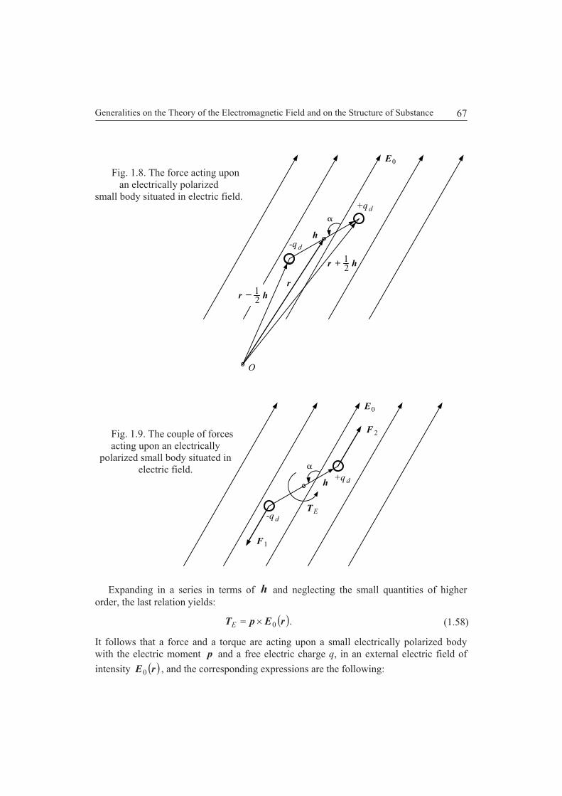
Generalities on the Theory of the Electromagnetic Field and on the Structure of Substance 67
Fig. 1.8. The force acting uponan electrically polarized
small body situated in electric field.
Fig. 1.9. The couple of forcesacting upon an electrically
polarized small body situated inelectric field.
Expanding in a series in terms of h and neglecting the small quantities of higherorder, the last relation yields:
.0 rEpTE (1.58)
It follows that a force and a torque are acting upon a small electrically polarized bodywith the electric moment p and a free electric charge q, in an external electric field of
intensity rE0 , and the corresponding expressions are the following:
h-q
+q d
d
E0
O
r
r + h12
r12 h
h
T E-q
+q d
d
E0
F
F
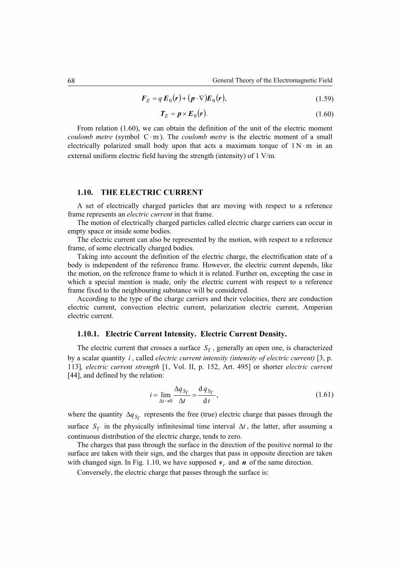
General Theory of the Electromagnetic Field68
,00 rEprEF qE (1.59)
.0 rEpTE (1.60)
From relation (1.60), we can obtain the definition of the unit of the electric momentcoulomb metre (symbol mC ). The coulomb metre is the electric moment of a smallelectrically polarized small body upon that acts a maximum torque of mN1 in anexternal uniform electric field having the strength (intensity) of 1 V/m.
1.10. THE ELECTRIC CURRENT
A set of electrically charged particles that are moving with respect to a referenceframe represents an electric current in that frame.
The motion of electrically charged particles called electric charge carriers can occur inempty space or inside some bodies.
The electric current can also be represented by the motion, with respect to a referenceframe, of some electrically charged bodies.
Taking into account the definition of the electric charge, the electrification state of abody is independent of the reference frame. However, the electric current depends, likethe motion, on the reference frame to which it is related. Further on, excepting the case inwhich a special mention is made, only the electric current with respect to a referenceframe fixed to the neighbouring substance will be considered.
According to the type of the charge carriers and their velocities, there are conductionelectric current, convection electric current, polarization electric current, Amperianelectric current.
1.10.1. Electric Current Intensity. Electric Current Density.
The electric current that crosses a surface S , generally an open one, is characterizedby a scalar quantity i , called electric current intensity (intensity of electric current) [3, p.113], electric current strength [1, Vol. II, p. 152, Art. 495] or shorter electric current
[44], and defined by the relation:
,d
dlim
0 t
q
t
qi
SS
t(1.61)
where the quantity Sq represents the free (true) electric charge that passes through the
surface S in the physically infinitesimal time interval t , the latter, after assuming acontinuous distribution of the electric charge, tends to zero.
The charges that pass through the surface in the direction of the positive normal to thesurface are taken with their sign, and the charges that pass in opposite direction are takenwith changed sign. In Fig. 1.10, we have supposed rv and n of the same direction.
Conversely, the electric charge that passes through the surface is:
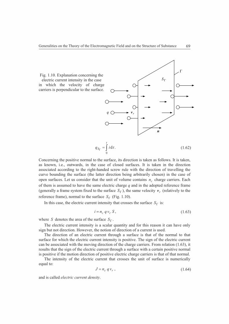
Generalities on the Theory of the Electromagnetic Field and on the Structure of Substance 69
Fig. 1.10. Explanation concerning theelectric current intensity in the case
in which the velocity of chargecarriers is perpendicular to the surface.
.d0
tiq
t
S (1.62)
Concerning the positive normal to the surface, its direction is taken as follows. It is taken,as known, i.e., outwards, in the case of closed surfaces. It is taken in the directionassociated according to the right-handed screw rule with the direction of travelling thecurve bounding the surface (the latter direction being arbitrarily chosen) in the case ofopen surfaces. Let us consider that the unit of volume contains cn charge carriers. Eachof them is assumed to have the same electric charge q and in the adopted reference frame(generally a frame system fixed to the surface S ), the same velocity rv (relatively to the
reference frame), normal to the surface S (Fig. 1.10).
In this case, the electric current intensity that crosses the surface S is:
,Svqni rc (1.63)
where S denotes the area of the surface S .The electric current intensity is a scalar quantity and for this reason it can have only
sign but not direction. However, the notion of direction of a current is used.The direction of an electric current through a surface is that of the normal to that
surface for which the electric current intensity is positive. The sign of the electric currentcan be associated with the moving direction of the charge carriers. From relation (1.63), itresults that the sign of the electric current through a surface with a certain positive normalis positive if the motion direction of positive electric charge carriers is that of that normal.
The intensity of the electric current that crosses the unit of surface is numericallyequal to:
,rc vqnJ (1.64)
and is called electric current density.
q v r
S
n
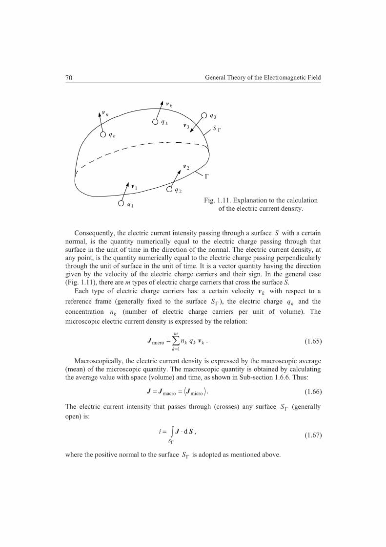
General Theory of the Electromagnetic Field70
Fig. 1.11. Explanation to the calculationof the electric current density.
Consequently, the electric current intensity passing through a surface S with a certainnormal, is the quantity numerically equal to the electric charge passing through thatsurface in the unit of time in the direction of the normal. The electric current density, atany point, is the quantity numerically equal to the electric charge passing perpendicularlythrough the unit of surface in the unit of time. It is a vector quantity having the directiongiven by the velocity of the electric charge carriers and their sign. In the general case(Fig. 1.11), there are m types of electric charge carriers that cross the surface S.
Each type of electric charge carriers has: a certain velocity kv with respect to a
reference frame (generally fixed to the surface S ), the electric charge kq and the
concentration kn (number of electric charge carriers per unit of volume). Themicroscopic electric current density is expressed by the relation:
.1
micro
m
k
kkk qn vJ (1.65)
Macroscopically, the electric current density is expressed by the macroscopic average(mean) of the microscopic quantity. The macroscopic quantity is obtained by calculatingthe average value with space (volume) and time, as shown in Sub-section 1.6.6. Thus:
.micromacro JJJ (1.66)
The electric current intensity that passes through (crosses) any surface S (generallyopen) is:
S
i ,d SJ (1.67)
where the positive normal to the surface S is adopted as mentioned above.
S
v
v
v
v
q
q
q
v k
n
k
n
1
q
q
3
2
3
2
1

Generalities on the Theory of the Electromagnetic Field and on the Structure of Substance 71
If the electric current density is normal to the surface S , and does not vary from onepoint to another, it follows:
,S
iJ (1.68)
where S is the area of the surface.Let us consider the electric charge of the charge carriers distributed in volume, with
the density v , in the adopted reference frame. The intensity of the electric current that
passes through the surface S is:
,dS
rvi Sv (1.69)
and the electric current density is:
.rv vJ (1.70)
In the microscopic theory of the electromagnetic field, the electric current intensityand the electric current density are derived quantities. In the macroscopic theory of theelectromagnetic field, one of the two quantities electric current intensity or currentdensity has to be introduced as a primitive (fundamental) quantity. For this purpose, theelectrochemical effect can be used.
In stationary regime (stationary operating conditions), the quantities voltage andintensity of the electric current may be denoted by small letters as well as by capitals.However, in other regimes, the notation has certain meanings.
From a microscopic point of view, as shown, the electric current is produced byelectrically charged microscopic particles in motion.
From a macroscopic point of view, it is accepted that the electric charge, as well as thesubstance, is distributed in space. The electric charges and therefore the electric currentmay be highly non-uniformly distributed on certain surfaces and may be concentrated oncertain surfaces, in a very thin film. Then, the macroscopic idealized case is considered inwhich the electric current is distributed in the form of a current sheet on each of thesesurfaces. Fig. 1.12 shows the trace of the surface dS with the current sheet on the figureplane.
Fig. 1.12. Explanation to the calculation of the linear current density. The cross-sectionsof the conductors (round wires) show that the carried currents enter the figure plane.
l
i
S d

General Theory of the Electromagnetic Field72
Correspondingly, it is possible to define a linear current density also called linear
current sheet and denoted by sJ or A :
.l
iAJ s (1.71)
Usually, it may be expressed as the number of ampere-turns per metre.
1.10.2. Conduction Electric Current
The electric charge carriers of the interior of a body of any substance are called free(electric charge) carriers if they are not permanently located within a certain atom ormolecule, and are called bound (electric charge) carriers if they are permanently locatedwithin one atom or molecule.
In certain cases, in dielectrics and semiconductors there are charge carriers (electronsor ions) which may have limited motions in the crystalline lattice. After such a motion, afree space remains, i.e., a space not occupied by particles of the crystalline lattice and it iscalled hole. After this free place is occupied by a neighbouring charge, a newneighbouring hole will appear.
This process can continue so that the row of holes, successively created, is equivalentto the displacement of the hole within the substance. The displacement of holes isanalogous to the motion of a charge carrier having the sign opposite to that of the chargesof the carriers the limited motions of which have produced the holes.
Therefore, if the holes are produced by limited displacements of certain electrons, thedisplacement of the hole is equivalent to the displacement of a positive charge. The freeplace is sometimes called hole or lacuna (pl. lacunae), as it is produced by thedisplacement of an electron or of an ion, respectively; however this distinction is notcompulsory, moreover it is rarely used.
The conduction electric current in a body is represented by the oriented motion of freeelectrons with respect to a reference frame attached (fixed) to that body.
According to the nature of the electric charge carriers (electrons, ions, holes), theconduction electric current may be referred to as electronic current, ion current, hole
current.Correspondingly, the conduction of the body under consideration is called electronic
conduction (e.g., for certain metals and semiconductors of N-type), ionic conduction(e.g., for electrolytes), and hole conduction (e.g., for semiconductors of P-type).
The macroscopic current density and the macroscopic current intensity can beexpressed by relations (1.66), (1.67).
1.10.3. Convection Electric Current
The convection electric current is represented by the motion of electrically chargedbodies with respect to a reference frame. Here, the electric current produced by themotion of a great number of electrically charged particles (for instance a flux of electronsor of protons) in empty space is included.
The macroscopic current density and the intensity of the convection electric currentcan also be expressed by relations (1.66) and (1.67).

Generalities on the Theory of the Electromagnetic Field and on the Structure of Substance 73
1.10.4. Polarization Electric Current
The polarization electric current is represented by the motion of bound electriccharges with respect to the centre of mass of atoms and molecules. Further, themacroscopic density and intensity of the polarization electric current will be calculated.
An open surface S bounded by a simple curve , both situated within a substanceelectrically polarized, will be considered. In the case of a variation of the electric fieldintensity, under the action of the forces determined by the electric field, the bound electriccharge carriers will change their position. Therefore, electric charge carriers pass throughthe open surface S , to very small distances. Hence, an electric current passes throughthe surface, and it is called polarization electric current.
The charges that produce the polarization electric current are just the charges thatproduce the electric polarization.
At a point of the surface S , we shall consider the physically infinitesimal volumev having the centre of mass at that point and containing a neutral system of electric
charges.The electric polarization, in any reference frame, with respect to which the substance
is at rest, is defined by relation (1.36 a) as:
,1
t1
n
i
ipiqv
rP (1.72)
where the summation refers to all electric charges which form neutral systems within thephysically infinitesimal volume v and the average value with respect to time is takenover a physically infinitesimal time interval. The quantities ir represent the positionvector in the considered reference frame. It is necessary to be mentioned that the positionvector of the centre of mass of the substance in the volume element v remainsunchanged even when the electric charge carriers change their position (because thepositive and negative charges move in opposite directions). Also, the mean concentrationof the bound carriers remains constant. At a modification of the electric field strength, asmentioned above, the positions of the electric bound charge carriers (the polarizationcharges) in the volume element v change. It follows:
,1
t1
n
i
ipi
tq
vt
rP(1.73 a)
thus:
.1
t1
n
i
ipiqvt
vP
(1.73 b)
The macroscopic density of the polarization electric current may be written:
,1
t1 tq
v
n
i
ipiP
PvJ (1.74)
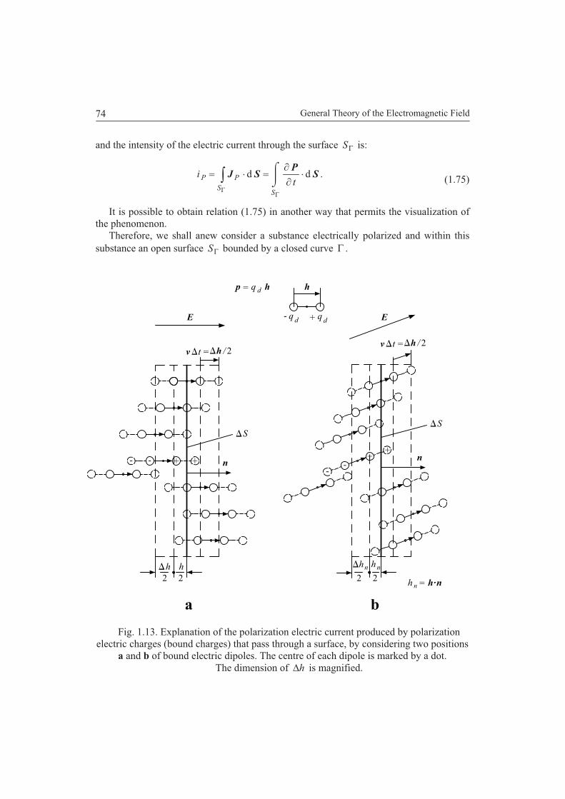
General Theory of the Electromagnetic Field74
and the intensity of the electric current through the surface S is:
.dd
SS
PPt
i SP
SJ (1.75)
It is possible to obtain relation (1.75) in another way that permits the visualization ofthe phenomenon.
Therefore, we shall anew consider a substance electrically polarized and within thissubstance an open surface S bounded by a closed curve .
Fig. 1.13. Explanation of the polarization electric current produced by polarizationelectric charges (bound charges) that pass through a surface, by considering two positions
a and b of bound electric dipoles. The centre of each dipole is marked by a dot.The dimension of h is magnified.
n
h
- q +
p q= h
h h
d
d qd
t / 2= hv
2 2
h
2
h
2h n =
n
/tv = h 2
E E
n n
h n
a b
SS
+ + ++
- --
-
Generalities on the Theory of the Electromagnetic Field and on the Structure of Substance 75
At a variation of the electric field strength, although the substance remains at rest withrespect to the reference frame, the bound electric charges modify their position, passingthrough the surface S and therefore produce an electric current. We shall express theintensity of the electric current in terms of the electric polarization.
For this purpose, we consider an element S of the surface S . We also assume thatthe various multipoles are replaced by equivalent dipoles, all identical to each other (Fig.1.13). The centre of each dipole is marked in the figure by a dot. This point remains atrest even when the bound electric charges move, since the substance is considered at rest.
We shall denote by pn the concentration of dipoles (i.e., the number of dipoles per
unit of volume) and by dq the positive charge of the dipole. It follows that under theaction of the electric field supposed as increasing in the direction of the arrow (Fig. 1.13),
the electric bound charges will move by the distance h2
1 in the time interval t with
the velocity th /2
1. Therefore, the dipoles will be elongated.
We shall consider, on the left side of the surface element S , the parallelepiped
having one base situated at the distance h2
1 from the surface element S and the height
h2
1 oriented towards the left side. The positive electric charges belonging to dipoles
that have their centres within the mentioned parallelepiped will pass through the surfaceS towards the right side with the velocity pv . The positive charge of each dipole which
has not its centre within the mentioned parallelepiped will not pass through the surface inthe time interval t , and hence will not contribute in producing an electric currentthrough that surface. Analogously, the negative electric charges from the right side of thesurface S will pass through the same surface towards the left side.
It results that through the surface SnS , the following electric current producedby positive bound charges will pass in the interval of time t :
.2
1
;pos
t
qni
p
pdp
hvv
Sv
(1.76)
For the negative charges, a similar expression can be obtained. It has to be taken intoaccount that the passage of an electric current produced by a number of negative chargesfrom the right to the left is equivalent to the passage of an electric current of an equalnumber of positive charges from the left to the right. It follows that the resultantpolarization electric current through the surface S , denoted by one of the symbols, Pi ,
pi , is:
.t
Sh
tqni dpP (1.77)

General Theory of the Electromagnetic Field76
Taking into account that the concentration of dipoles does not change because thecentres of the dipoles remain at rest, it follows:
.t
SP
Sht
qnt
i dpP (1.78)
From relation (1.78), it follows that:
SS
PPt
i .dd SP
SJ (1.78 a)
The same result will be obtained if it is considered that a rotation of dipoles isproduced under the action of the external electric field.
From the explanation above, it follows that the polarization current cannot be a steady-state direct current, since the displacement of bound charges is limited. Only polarizationcurrent varying with time can exist.
1.10.5. Amperian Electric Current (Molecular Electric Current)
The motion of an electric charge carrier along a closed way of sub-moleculardimensions is referred to as molecular or Amperian electric current. The concept ofmolecular current was introduced by Ampère for the explanation of the magnetization ofbodies based on electric currents, that is why the molecular currents are also calledAmperian currents.
The following simple models can be considered. The Amperian (molecular) electriccurrents are essentially represented by the orbital and spin motion of electrons. Indeed,each electron describes an orbital trajectory about the nucleus of the atom. The orbitaltrajectory is assumed as having the shape of a circumference, or more precisely, that of anellipse. Moreover, it is also assumed that each electron turns about an axis passingthrough its centre. This rotation may be of any sense, for some electrons, e.g., clockwise,of opposite sense, i.e., counter-clockwise, for the others. This electron movement is calledspin motion.
Further on, the density and the intensity of the molecular current will be calculated.Details on the motion of electrons and more precise models can be found in worksdevoted to this subject. Certain details are given in the work [26]. For the sake ofsimplicity, all Amperian electric current will be supposed identical to each other havingthe intensity Amperi and a circular trajectory of radius 0r and normal n .
Within a substance in which there are Amperian (molecular) electric currents, weconsider (imagine) an open surface S bounded by a closed curve (Fig. 1.14).
We shall calculate the macroscopic intensity of the Amperian electric current throughthis surface. The electric current intensity is:
,AmperS
M ii(1.79)

Generalities on the Theory of the Electromagnetic Field and on the Structure of Substance 77
where the summation refers to all Amperian currents the trajectories of which intersectthe surface S .
It is worth remarking that the intensity of a microscopic current occurs in thecalculation of the sum of relation (1.79) only if that current crosses once the surface S
(if it crossed twice the surface, its contribution to the total current would be zero). Hence,only the Amperian currents that link the curve contribute to the sum. We shallcalculate the macroscopic Amperian current given by the sum:
,AmperiiM (1.80)
where the summation refers to all Amperian currents that link the curve .Let us consider that along a short portion l of the curve , the orbits of the
Amperian currents are parallel with each other and their surfaces perpendicular to theconsidered portion of the curve . The Amperian current concentration (i.e., the numberof Amperian currents per unit of volume) in this region will be denoted by 0n . TheAmperian currents that link the arc l of the curve are contained inside a right cylinderhaving as axis the mentioned segment l approximated by a straight-line segment, andthe diameter 02 r , where 0r is the radius of the orbit of an Amperian current. Thus:
,0Amper0Amper lSinil
(1.81)
where 0S denotes both the surface of the orbit of an Amperian current and the area of thecross-section of the cylinder above. If the normal n to the surface of the orbit of the
Fig. 1.14. Orbits of the Amperian (molecular) currents and thesurface through which macroscopic electric currents are passing.
For the sake of clearness, the orbits are magnified.
2 r 0
i
S
2 r 0l
Amperian
General Theory of the Electromagnetic Field78
Amperian current forms a certain angle with the arc element l , it follows:
.0Amper0Amper lSinil
(1.81 a)
The calculation performed for a single curve can be repeated for several closedcurves very closed to each other. These curves form a bundle that occupies the domain inthe form of a closed tube (pipe). The cross-section of this tube must be small enough, sothat together with the line element l , it shows a physically infinitesimal volume v .
We shall denote:
,0Amper0 Sm i (1.82)
quantity called magnetic moment of an Amperian current or Amperian magnetic moment,and:
,1
00
t
0 mmM nv v
(1.83)
where v represents the physically infinitesimal volume. The sum of magnetic momentsof Amperian currents of a volume of any substance may be different from zero. The stateof the substance in this case is referred to as magnetization state. From a microscopicpoint of view, the magnetic moment is a secondary (derived) quantity. From amacroscopic point of view, the magnetic moment has to be introduced experimentally asa primitive (fundamental) quantity. The manner of introducing this quantity is based onthe ponderomotive forces acting on a magnetized small body situated in a hollow cavitywithin the substance. The vector quantity M defined by relation (1.83) is calledmagnetization. In the case of a uniform distribution, it represents, the average value, overa physically infinitesimal time interval, of the vector sum of magnetic moments of a unitof volume. Generally, it represents the ratio of the sum of magnetic moments, of aphysically infinitesimal volume, to the magnitude of this volume.
Instead of the vector quantities, Amperian magnetic moment m and magnetizationM , corresponding to expressions (1.82) and (1.83), there are also used the quantitiesCoulombian magnetic moment jm and magnetic polarization jM defined by the
following expressions that contain the constant 0 :
,000 mm j (1.84)
,0 MM j (1.85)
where the quantity 0 represents a constant called the magnetic constant also termedpermeability of vacuum, which will be explained in Section 2.4.
The quantity jM is denoted, according to [44], by the symbol J but we shall not use
it, in order to avoid any confusion, because in this work the electric current densitydenoted by the same symbol also occurs. Another symbol for denoting the same quantity,according to [44], is iB and it is called intrinsic magnetic induction.
Generalities on the Theory of the Electromagnetic Field and on the Structure of Substance 79
If the quantities jm and jM are used, then certain relations, referring to the magnetic
polarization state, show a symmetrical form with the corresponding relations referring tothe electric polarization state.
Correspondingly, we obtain the volume density of the fictive (fictitious) magnetic
charge:
,div MMv (1.86)
called volume density of the (fictive) magnetization charge, and
,div jmv M (1.87)
called volume density of the (fictive) magnetic polarization charge.The relations (1.81), (1.83) yield:
,dAmper lMi (1.88)
and taking into account relation (1.80), it results that:
.d lMMi (1.89)
The macroscopic density of the macroscopic Amperian electric current, denoted byone of the symbols AJ , aJ , MJ , mJ , can be obtained by using the Stokes theorem asfollows:
.dcurlddSS
AMi SMlMSJ (1.90)
It results that:
.curl1
curl0
jaA MMJJ (1.91)
The magnetization M can be decomposed into the sum of two components. The firstone exists even in the absence of external causes and is determined by the nature of thesubstance. This component is called permanent magnetization and it is denoted by pM .
The second one appears only under certain external causes (e.g., a magnetic field) and isdetermined by these causes and the nature of the substance. This component is calledtemporary magnetization and it is denoted by tM . Therefore, for the components of thevectors magnetization and magnetic polarization, respectively, we obtain:
,tp MMM(1.92)
.jtjpj MMM (1.93)
In certain situations, each of the two components above may be zero.
General Theory of the Electromagnetic Field80
1.11. LAW OF FREE (TRUE) ELECTRIC CHARGE CONSERVATION
1.11.1. Integral Form of the Law
Let us consider any closed surface passing only through insulating materials, sothat the surface is not crossed by electric currents, then the total electric free charge of theinterior of the surface remains constant:
.constq (1.94)
This relation, called law of electric charge conservation, is valid regardless of thephenomena produced in the interior of the surface .
If an electric conduction current of intensity i passes through the closed surface ,leaving this surface, then the integral form of the law is modified as follows:
.d
d
t
qi (1.95)
This last expression of the integral form of the law of electric charge conservation alsofollows from the magnetic circuital law subsequently treated; however the first integralform of the law (1.94) does not result from the magnetic circuital law.
1.11.2. Local Form of the Law
The relation (1.95) can be modified as follows:
,dd
dd
V
v vt
SJ (1.96)
where the quantity J represents the density of the current passing through the surface and the quantity v represents the volume density of the electric free charge.
Two cases will be examined: Surface at rest with respect to the reference frame;surface in motion with respect to the reference frame.
1º Surface at Rest Relatively to the Reference FrameIn a reference frame at rest with respect to the surface , the operation of
differentiation can be introduced under the integral sign and it follows:
.ddV
v vt
SJ (1.97)
By transforming the surface integral into a volume integral (Gauss-Ostrogradskitheorem), we obtain:
.dddivV
v
V
vt
SJ (1.97 a)

Generalities on the Theory of the Electromagnetic Field and on the Structure of Substance 81
Since the last relation is valid for any surface Σ , it results that:
,divtv
∂ρ∂
−=J (1.98 a)
or
.0div =+∂ρ∂
Jtv (1.98 b)
Relation (1.98 b) represents the local form of the law of free (true) electric chargeconstancy for a medium to which the surface Σ is attached (fixed) and that issimultaneously at rest with respect to the reference frame.
2º Surface in Motion with Respect to the Reference FrameIf the surface Σ is moving with respect to the reference frame and the various points
of this surface have any velocity rv with respect to the reference frame, then whencalculating the derivative:
,ddd∫Σ
ρV
v vt (1.99)
it is necessary to take into account that two terms will occur: One term is obtainedsupposing that the surface is at rest, and the quantity vρ varies with time; the second termis obtained supposing that the surface is moving and the quantity vρ does not vary withtime, i.e., the procedure is the same as for the calculation of the derivative of composedfunctions.
The first term is:
.d vt
V
v⎮⌡⌠
∂ρ∂
Σ
(1.100 a)
The second term is given by the relation:
,dd1
12 ⎥⎥⎥
⎦
⎤
⎢⎢⎢
⎣
⎡ρ−ρ
Δ ∫∫ΣΣ V
vV
v vvt
(1.100 b)
where Σ=Σ1 and 2Σ represent the two consecutive positions of the surface Σ (Fig.1.15), and
1ΣV and 2ΣV are the domains (volumes) bounded by the surfaces 1Σ and 2Σ ,
respectively. The surface 1Σ denotes the first position and the surface 2Σ denotes thesecond consecutive position after the displacement of every point of the surface Σ withthe segment tr Δ⋅v .
Considering Fig. 1.15, it follows that the variation of the integral expressed by relation(100 b) is given by the integral:

General Theory of the Electromagnetic Field82
,d
dV
v v(1.101)
that has to be calculated over the domain (volume) bounded by the closed surface d .
The closed surface d is determined by the two consecutive positions 1 and 2 of the
closed surfaces. Fig. 1.15 shows an element of the domain bounded by the surface d .This element is a curvilinear parallelepiped. From the examination of Fig.1.15, it follows:
.tv rvS (1.102)
By replacing the volume element in expression (1.101) and integrating over allelements Sd , hence over the whole surface d , we obtain:
.dd
dd
tv rv
V
v vS(1.103)
Therefore, the derivative of the considered integral is:
,dddd
d
V
rvv
V
v vt
vt
Sv (1.104)
and by replacing in relation (1.96), it follows:
.dddV
rvv vt
SvSJ (1.105)
By transforming the surface integrals into volume integrals, the last relation becomes:
.ddivdddivV V
rvv
V
vvt
v vJ (1.106)
Since the last relation should be valid for any surface , it results that:
.divdiv rvv
tvJ (1.106 a)
Fig. 1.15. The displacement of anelement of the surface in the two
consecutive positions anddetermining the surfaces 1 and 2 .
v r tS
2
1
Generalities on the Theory of the Electromagnetic Field and on the Structure of Substance 83
The last relation yields:
,0div rvv
tvJ (1.107)
that represents the local form, i.e., the differential form, for a medium (to which thesurface is attached) in motion with the velocity rv with respect to the reference frame.
The quantity J represents the current density in a reference frame attached (fixed) to
an element of the surface and the derivative t
v is expressed in the reference frame
with respect to which the surface is moving. Thus rv vJ represents the currentdensity with respect to the reference frame at rest, relatively to which the surface ismoving. With this remark, relation (1.107) can be obtained directly from relation (1. 98 b)by replacing, correspondingly, the electric current density.
1.12. THE LAW OF ELECTRIC CONDUCTION. THE LOCAL FORM.
The magnitude of the density of the conduction electric current at a point of anymedium depends on the strength of the electric field in the large sense at this point, andon the nature of the medium.
In the case of any isotropic medium, the density vector of the electric current, at apoint, has the same direction as the vector of the electric field strength at the same point,and is given by the relation:
,lEJ (1.108)
where is a positive quantity. The quantity is called electric conductivity and isdepending on the medium nature, thus a material quantity. The quantity:
,1
(1.109)
is called electric resistivity.Macroscopically, relation (1.108) can be obtained only in an experimental way. In the
macroscopic theory, this relation is a material law, also termed constitutive law, and isreferred to as the electric conduction law or the general Ohm law. In metallic conductors,the electric resistivity depends, generally, on temperature.
The expression of the electric resistivity can be expanded in a Taylor series in terms oftemperature:
....!2
1
!1
1 22
2
00
00
(1.109 a)
General Theory of the Electromagnetic Field84
For relatively small variation, by neglecting the small terms of higher order, thedependence is a linear one:
,1 000 (1.110)
,1
000 (1.110 a)
where the following symbols have been used:
– electric resistivity at temperature ;
0 – electric resistivity at temperature 0 ;
0 – raising coefficient of resistivity with temperature.
The values of the resistivity and of the raising coefficient of resistivity withtemperature are given, according to the experimental results, in tables.
The resistivity of a metal usually increases with temperature, even during the metalmelting. However, certain metals like bismuth, antimony, gallium show a decrease oftheir density during their melting, and their resistivity diminishes during their melting. Inthe microscopic theory of the electromagnetic field, relations (1.108) and (1.110) can bededuced starting from the general law of the electromagnetic field.
In the case of anisotropic media, the direction of the vector J is not the same withthat of the vector lE . However, in these media, it is possible to determine a system ofthree-orthogonal axes called principal axes, along which, the anisotropic medium behaveslike an isotropic one. In the case of these media, the electric conduction law, in the localform, can be written in the form:
lEJ , (1.111)
where the quantity is the tensor of the electric conductivity. Relations (1.108) and(1.111) have a general character being valid in the cases when the quantities varies withtime.
In dielectrics (substances with bad conducting properties) and in semiconductors,generally, the dependence between the density of the conduction electric current and theelectric field strength is not a linear one. However, in these cases, the same manner ofexpressing the law is used. Then, the expression of the law is equivalent to theexpression, for each considered substance, of the dependence lEfJ and JfEl .
The law is also applicable, with a good approximation, to electrolytes.In the framework of the microscopic theory, using a simplified model, the relation
(1.108), can be derived as follows. The electric current flowing in a body is produced bythe oriented displacement of electric charge carriers under the action of external forces.The collision of the charge carriers with the ions and atoms of the body opposes to theoriented displacement of the charge carriers. Hence, the substance of the body presents acertain resistivity to the electric current. The relation (1.108) that expresses thisphenomenon can be deduced directly from the equation of motion of the electric chargecarriers moving under the action of the forces which occur [23, Vol. II, p. 30].

Generalities on the Theory of the Electromagnetic Field and on the Structure of Substance 85
1.13. THE ELECTRIC FIELD STRENGTH OF ELECTRICCHARGES IN VACUO. ELECTRIC CONSTANT (ELECTRICPERMITTIVITY OF VACUUM).
1.13.1. COULOMB Formula
Let us consider two small bodies indicated by numbers 1 and 2, with the electriccharges 1q and 2q respectively, at rest in a reference frame and situated at points A andP at a relatively great distance (compared with the dimensions of each body) from eachother. Therefore, the charges 1q and 2q can be referred to as point-like charges.
The vector quantity 12r represents the distance between the two bodies, oriented fromthe body 1 towards the body 2, like in Fig. 1.16.
The force exerted upon the body 2 with the electric charge 2q due to the body with
the electric charge 1q is given by the expression:
,12
122
12
21021
rr
qqk
rF (1.112)
that represents the Coulomb formula in the case of empty space (i.e., vacuum).At the time when it was experimentally established, relation (1.112) had a very
general character and has been referred to as the Coulomb law. At present, it is also calledthe Coulomb theorem. From expression (1.112) and Fig. 1.16, it results that the directionof the force is so that the charges of the same sign repel each other, and the charges ofopposite sign attract each other. The Coulomb formula can be used for introducing thenotion of true (free) electric charge.
The quantity 0k is a universal constant referring to vacuum (free space, empty space),i.e., a physical quantity independent of the nature of the bodies under consideration and ofall other physical quantities, dependent on the chosen system of units.
In the SI system of units, which is a rationalized system, instead of the constant 0k the
quantity 0 is used, and the relation between the two quantities is:
.4
1
00k (1.113)
The quantity 0 is also a universal constant referring to vacuum and is calledpermittivity of vacuum or electric constant, and in the SI system has the value:
Fig. 1.16. Explanation concerning the Coulomb formula.
(1) ( 2 ) q2q1
r 12A P F 21

General Theory of the Electromagnetic Field86
,m/F1094
190 (1.114)
expressed in farad / metre (symbol F / m); the units of measure will be explained in Sub-section 3.13.3.
If instead of relation (1.114), other values are adopted for the constant of relation(1.112), other systems of units of measure of the electromagnetic quantities will beobtained. The expression of the Coulomb formula, in vacuo, in the SI system of units is:
.4
1
12
122
12
21
021
rr
qq rF (1.115)
As mentioned in Sub-section 1.6.2, the unit of measure of electric charge is calledcoulomb. According to relation (1.115), the coulomb is the value of the point-like charge
that exerts a force of N109 9 upon another identical point-like charge placed at thedistance of 1 m from the first point-like charge and very far from any other body.
According to relation (1.17), it results that the electric field strength produced by thecharge 1q at the point 2 (Fig. 1.16) has the expression:
.4
1
12
122
12
1
021
rr
q rE (1.116)
Relation (1.116) is also termed Coulomb formula, relation or theorem, respectively.
1.13.2. Utilization of the Principle of Superposition
For obtaining the force acting on a point-like charge, in many cases it is useful toapply the principle of superposition. Therefore, for obtaining the force acting upon apoint-like charge q, due to other point-like charges niqi .,..,1 , the forces
corresponding to the pairs of charges 1, qq ; 2, qq ; . . .; nqq, will be calculated
separately and the forces 1F , 2F , . . ., nF will be obtained. The resultant force exertedupon the point-like charge q situated at any point A is:
.1
n
i
iFF (1.117)
Correspondingly, the electric field strength at point A produced by the point-likeelectric charges niqi .,..,1 , the charge q being absent, is:
.1
n
i
iEE (1.118)

Generalities on the Theory of the Electromagnetic Field and on the Structure of Substance 87
1.13.3. The Electric Potential Produced by Electric Charges at Rest
We shall calculate the electric field strength produced at any point N , calledobservation point or field point, by whatever point-like charge denoted here by q that is
placed at any point M called source point. We shall denote MNr . The electric fieldstrength at the point N is given by relation (1.116) and can be written in the form:
,grad4
1grad
4
1
02
0
Vr
q
rr
q rE (1.119)
where the following symbol has been used:
,4
1
0
Cr
qV (1.120)
where C is an arbitrary constant. The scalar quantity V is called potential and because, inthis case, it is produced by electric charges at rest, it is termed electrostatic potential. Theminus sign in the right-hand side of relation (1.119) appears due to the followingconvention accepted in the theory of the electromagnetic field. According to thisconvention, the displacement direction of the particles with positive electric charge isoriented from the regions of a higher potential towards the regions of a lower potential.
Hence, the direction of the electric field strength vector and the direction of the linesof electric field are oriented from the regions of a higher potential towards the regions ofa lower potential. This direction is opposite to that of the vector Vgrad , since the vector
Vgrad is oriented along the direction along which V increases most rapidly.According to the principle of superposition, the electric field strength produced at any
point N , by n point-like electric charges ).,..,1( niqi , each of them placed at the
point iM , is:
,4
1grad
4
1
1 012
0
n
i i
in
i i
i
i
i
r
q
rr
q rE (1.121)
where NM iir , and the potential is:
,4
1
1 01
n
i i
in
i
i Cr
qVV (1.122)
where:
.4
1
0i
i
ii C
r
qV (1.122 a)
If besides the point-like electric charges it is a distributed electric charge, then, bydecomposing the electric charge distribution in elementary electric charges, thedistribution of electric charges may be replaced by sets of point-like charges and relationsof the form (1.121) and (1.122) can be applied.
General Theory of the Electromagnetic Field88
In the general case, in which in the whole infinite empty space (i.e., in vacuo) there aren point-like electric charges and volume, surface and line electric charge distributions, theexpression of the potential can be written:
,ddd4
1
10
Clr
Sr
vrr
qV
qqq C
l
S
sn
iV
v
i
i (1.123)
and the electric field strength is:
.ddd4
1grad
221
220
lrr
Srr
vrrrr
qV
qqq C
l
S
sn
iV
v
i
i
i
i rrrrE
(1.124)
The electrostatic potential is a scalar function introduced in order to simplify the studyof the electrostatic field and generally has not a physical interpretation, excepting thedifference of the potentials at two points that can be related to a work, as it will be furtherexplained.
Therefore, in the applications in which the distribution of electric charges in vacuo isgiven, and the calculation of the electrostatic field is required, the following procedure ispossible: To calculate successively the potential by relation (1.123) and then the gradient.This way represents, in many cases, a much simpler solution than the direct calculationby relation (1.124).
The electrostatic potential is useful for the calculation of the line-integral of theelectrostatic field strength between two points, referred to as: a) potential difference
between the two points, b) voltage between the two points or c) electric (electrostatic, inthe present case) tension between the two points.
The expression of the line integral is:
N
M
CMNU ,d lE (1.125)
but, in the case of the electrostatic field, we may write:
,gradz
V
y
V
x
VV kjiE (1.125 a)
and
.dddd zyx kjil (1.125 b)
Thus:
.dddd zz
Vy
y
Vx
x
VlE (1.125 c)

Generalities on the Theory of the Electromagnetic Field and on the Structure of Substance 89
It follows:
,ddddN
M
N
M
CMN Vzz
Vy
y
Vx
x
VU (1.126)
and taking into account that the expression under the integral sign is a total differential, itresults that:
.NMCMN VVU (1.127)
It results that, in the case of the electrostatic field, the potential difference (voltage)between two points is independent of the curve along which it is calculated and is equalto the difference of the electrostatic potentials at the two points.
1.14. THE ELECTRIC FLUX LAW IN VACUO
Let us consider a closed surface situated in vacuo, and in its interior a point-likecharge q (that may be referred to as source charge). The electric field strength at a pointof the surface can be obtained by relation (1.119), using the same symbols, and it isgiven by the following expression:
.4
12
0 rr
q rE (1.128)
We shall calculate the flux of the electric field strength vector through the surface .
Fig. 1.17. Explanation concerning the electric flux law in vacuo.
+q
r02
n
0r
n
O
N
r
0
General Theory of the Electromagnetic Field90
We have:
.d4
1d
20
E Sr
SErr
q(1.129)
We surround the point at which is the point-like charge, by a sphere of surface 0
having its centre at that point and any radius 0r (assumed generally small but thisassumption is not necessary). Then, we shall consider the surface obtained by the unionof surfaces and 0 . We obtain:
.00v (1.130)
We shall calculate the flux of the vector E through the surface 0v . Having in viewthe positive direction of the positive normal to the last surface, as shown in Fig. 1.17, weobtain:
.ddd
00
0E SESESE
v
v (1.131)
For the exterior surface , we have:
.dE SE (1.131 a)
For the interior surface 0 , hence that of the sphere, we have 0
0
r
rn , and
consequently:
.44
1d
4
1
d4
1dd
0
202
002
00
0
0
0
02
00E
0
0 00
0
qr
r
qS
r
q
Srrr
qS
rrnESE
(1.131 b)
At the same time:
.ddivd
00
0E v
vv
v
V
ESE(1.132)
But in the considered domain 0
V , which does not contain the singular point 0r , we
have:
.0div4
div3
0 r
q rE (1.133)
Introducing into relation (1.131), the expressions (1.131 a) and (1.131 b), and takinginto account relations (1.132) and (1.133), we obtain:

Generalities on the Theory of the Electromagnetic Field and on the Structure of Substance 91
.d0
qSE (1.134)
Formula (1.134) expresses the integral form of the electric flux law in vacuo, in thecase of a single point-like charge.
Formula (1.134) can also be directly established starting from relation (1.129), takinginto account that the quantity:
Sr
dd3r
(1.135)
represents the solid angle subtended at the point O (i.e., at 0r ) by the surface elementSd . Therefore, the solid angle is obtained as follows. Let O and S be the given
point and surface, respectively. Let 0 be a spherical surface having its centre at the
point O and any radius 0r . Let us consider the conical surface obtained when a half-straight-line having its starting point at O is moving along the closed curve that boundsthe surface S . Let 0S be the surface determined by the intersection of the conicalsurface with the spherical surface. Then, the solid angle subtended at the point O by thesurface S is defined as:
.2
0
0
r
S(1.136)
Immediately, it follows that if S is a closed surface containing the point O, then 0S
will be the whole surface of the sphere 0 , and the solid angle will be 4 . It is the solid
angle subtended at the point O by the surface of the sphere. If 0S were smaller than thewhole surface of the sphere, the solid angle subtended at the point O would be less than4 .
The concept of solid angle is an extension of the notion of plane angle, from the PlaneGeometry, to the notion of solid angle, in the Solid Geometry. As shown, the definitionsare analogous.
Also, as shown, if the point O is contained by the closed surface , then the surfaceS is to be replaced by that whole surface and the solid angle subtended at the point O
by the closed surface will be 4 .If the point O is just on the closed surface , then the surface S is to be replaced by
that whole surface and we shall consider the point O as tending from a neighbouringposition to the final one, on the surface . It results that, in this case, the solid anglesubtended at the point O by the closed surface will be 2 .
If the point O is outside the closed surface , anew the surface S is to be replacedby that whole surface. In this case, the conical surface above will be tangent to the closedsurface and consequently divides the whole closed surface into two parts. The value(area) of the surface on the sphere 0 corresponding to those two parts will have thesame absolute value but opposite signs. The different signs are determined by the
General Theory of the Electromagnetic Field92
opposite directions of the positive normal to each of the two surface parts. Therefore, inthis case, the solid angle subtended at the point O will be 0 .
It results that the flux of the vectors E through the surface element S is:
.4
d0
q
S
SE (1.137)
If inside the surface , there are several point-like electric charges, then, inaccordance with the principle of superposition and relation (1.118), expression (1.137)remains valid provided that, in the right-hand side, the sum of all point-like electriccharges is introduced.
If inside the surface, there are distributed electric charges, then, by decomposing theelectric charge distributions into elementary electric charges, the electric chargedistributions can be replaced by sets of point-like electric charges and relation (1.137)remains valid.
It follows that, generally, for a closed surface , the following expression can bewritten:
,d0
qSE (1.138)
or
,dd0 qSDSE (1.139)
,0 ED (1.139 a)
where the quantity q represents the total free (true) electric charge of the interior of thesurface and D is called the electric flux density in vacuo.
The expressions (1.138) and (1.139) represent the integral form of the electric flux law
in vacuo.The electric charge of the inside of the surface can be expressed in terms of the
electric charge volume density:
,d vq
V
v (1.140)
and relation (1.139) becomes:
.dd0 v
V
vSE(1.141)
By the aid of the transformation relation of a volume integral into a surface integral(Gauss-Ostrogradski theorem), we obtain:
.dddiv0 vv
V
v
V
E(1.141 a)
Generalities on the Theory of the Electromagnetic Field and on the Structure of Substance 93
Since the last relation can be written for any volume domain V , it results that:
,div0 vE (1.142)
which is the local form of the electric flux law in vacuo.By replacing relation (1.124) in (1.142), in the case in which only a volume electric
charge distribution exists, it follows:
0
graddiv vV (1.143 a)
or
.0
2 vV (1.143 b)
In the framework of the macroscopic theory, the electric flux law is a general law. Inthe framework of the microscopic theory, it can be derived as above, as a theorem. Forthis reason, the above law is also called the electric flux theorem as well as the Gauss
theorem.The integral form of the electric flux law can be expressed as follows: The flux of the
electric field strength through a closed surface, situated in vacuo, is proportional to thesum of all electric charges belonging to the volume delimited by this surface.
In the case in which there is a single point-like electric charge, but situated on thesurface , then, in relation (1.138) or (1.139), the right-hand side will be multiplied bythe factor 21 . The reason has been shown above (considering the solid angles) and itconsists in the fact that instead of a sphere surrounding the point-like charge (Fig. 1.17), itis a half-sphere (hemisphere) that occurs.
The charges from the outside of the closed surface do not occur in the expression ofthe electric flux law.
1.15. THE SI UNITS OF: ELECTRIC CHARGE, ELECTRICMOMENT, ELECTRIC TENSION, ELECTRIC FIELDSTRENGTH, ELECTRIC CURRENT.
In the publications concerning the SI system of units, a set of definitions of the unitsof measure is given. For the same units, various definitions can be used as required. In thepresent work, each occurring unit is defined employing only relations and unitspreviously introduced.
1.15.1. The Unit of Electric Charge
The SI unit of electric charge may be established in accordance with the Coulomb
formula and is called coulomb (symbol C). The electric charge of a conducting small
body that exerts a force of N109 9 upon another identical body having an identical

General Theory of the Electromagnetic Field94
electric charge, in vacuo, at the distance of 1 m from the first body, and very far from anyother bodies, is called coulomb. The definition of this unit has been examined in the Sub-section 1.13.1.
The units of volume, surface and line density corresponding to relations (1.7), (1.8)
and (1.9), respectively, are the following: coulomb per cubic metre (symbol 3m/C ),
coulomb per square metre (symbol 2m/C ) and coulomb per metre (symbol m/C ).
1.15.2. The Unit of Electric Moment
The SI unit of electric moment results from relation (1.26) and is called coulomb-metre (symbol mC ). Coulomb-metre is the electric moment of an electrically polarizedsmall body upon which a maximum torque of mN1 is exerted in an electric field havingthe strength of m/V1 . The definition of this unit has been examined in Sub-section1.9.6.
The unit of electric induction and electric polarization is called coulomb per square
metre (symbol 2m/C ) and will be explained in Sub-section 3.13.1.
1.15.3. The Unit of Electric Tension
The SI unit of the quantities: electric potential difference, electric tension,electromotive force, and in general the integral of the electric field strength along a curveis the volt (symbol V).
The definition of this unit can be given according to relation (1.22). The line-integralof the electric field strength, along a curve, in any reference system, between two points,has the value of 1 volt, in the following case. Let a small body with the electric charge of1 C move along that curve in an electric field, with a very small velocity. Also, duringthis motion, let the forces due to the electric field and exerted upon the body above do awork of 1 J. In this case, the integral above will be equal to 1 V.
The small velocity is required for the definition of the electric field to be valid in theconsidered reference frame.
After the unit of the electric potential difference has been adopted, according torelation (1.23 a), the unit of the electric field strength can be deduced and is called volt
per metre (symbol m/V ). The strength of a uniform (homogeneous) electric field is of1 m/V if the electric potential difference between two points situated at a distance of
m1 along a direction parallel with the direction of the electric field strength is of V1 .
1.15.4. The Unit of Electric Field Strength
At the same time, another definition of the electric field strength can also be givenafter having adopted the unit of electric charge. In accordance with relation (1.17), theelectric field strength in vacuo, at any point, has the value of m/V1 if at that point, the
electric field exerts a force of N1 upon a conducting small body having the electriccharge of C1 .

Generalities on the Theory of the Electromagnetic Field and on the Structure of Substance 95
1.15.5. The Unit of Electric Current Intensity
The SI unit of the intensity (strength) of the electric current is called ampere (symbolA). The electric current constant with time that passes through any surface has the valueof 1 A (ampere) if through that surface an electric charge of 1 coulomb passes in a time of1 second:
.s1
C1A1 (1.144)
Another form for expressing the unit in the SI system of a certain quantity will beshown for the case of the unit of electric current, as follows:
.1s1
C1
][1
][1][1 SI A
t
qI (1.145)
The unit of the electric current density is called ampere per square metre (symbol2m/A ). Since this unit is small, in numerous practical applications, a multiple of this
unit is used, namely ampere per square millimetre (symbol 2mm/A ). When the electric
current density is introduced in computation expressions in 2mm/A , it is necessary tomake the involved transformations.
The unit of the linear current density is the ampere per metre (symbol m/A ).

General Theory of the Electromagnetic Field96

2. INTRODUCTION OF THE STATE QUANTITIES OFTHE ELECTROMAGNETIC FIELD IN VACUO
The state quantities of the electromagnetic field can be introduced (i.e., defined) eitherby experimental way or by using the expression of transformation of forces when passingfrom one reference frame to another that is moving with respect to the first one. Firstly,the second way will be used, and further the first way will be presented. Each mannerrequires certain derivations. The manner of presentation used for the first way is based onseveral works [23], [11], [13], [25], [40], [41].
2.1. THE LAW OF PONDEROMOTIVE ACTION UPON APOINT-LIKE ELECTRIC CHARGE AT REST IN AN INERTIALREFERENCE FRAME
The electric charge of any body, according to the non-correlative definition of Sub-section 1.6.2, will be considered as independent of the velocity of the body. Thisassumption is supported by experimental facts mentioned in the above Sub-section.
We shall consider a point-like electric charge in vacuo in a reference frame
oooo ,, zyxK , considered as the original frame, and another reference frame
1111 ,, zyxK that is moving, at a constant velocity, relatively to the first referenceframe. The original reference frame is indicated by the suffix “o”, in order to avoid anyconfusion with the suffix “0” of 0 and 0 .
Any reference frame may be considered, but further on, only inertial reference frameswill be examined.
We shall recall the meaning of inertial reference frame, and we shall make someremarks.
Inertial reference frame is called any reference frame, with respect to which, threematerial points, very distant from each other and from other bodies, and moving indifferent, non- parallel planes, describe straight-line trajectories.
All inertial systems are equivalent to each other, from the point of view of mechanicalphenomena. Indeed, all the laws of Classical Mechanics (e.g., inertial law, action andreaction law, fundamental law of Dynamics) have the same expression in any inertialreference frame. The inertial reference frames are in a uniform translation motion.
The expression of the law of ponderomotive action, in any reference frame K, exertedupon a point-like charge q, at rest, in this reference frame is:
.EF q (2.1)
The expression of the law of ponderomotive action is:
,oo EF q (2.2 a)

General Theory of the Electromagnetic Field98
in the reference frame oK if the point-like charge is at rest in this reference frame and:
,11 EF q (2.2 b)
in the reference frame 1K if the point-like charge is at rest in this reference frame.
The vector quantities oE and 1E represent the electric field strengths in the reference
frames oK and 1K , respectively.If the point-like charge (or the body represented by this charge) is moving relatively to
the reference frame, then the law of ponderomotive action is different from that presentedabove. In this case, the law can be established either by the generalization of experimentalresults or by using certain expressions from Mechanics established in the Special Theoryof Relativity.
2.2. DERIVATION OF THE EXPRESSION OF THE LAW OFPONDEROMOTIVE ACTION UPON A POINT-LIKE ELECTRICCHARGE THAT IS MOVING RELATIVELY TO AN INERTIALREFERENCE FRAME
The expression of the law of ponderomotive action upon a point-like charge that ismoving with respect to an inertial reference frame can be established by using certainassumptions (hypotheses) from Mechanics established in the Special Theory ofRelativity.
The used hypotheses are the following:1. In an inertial reference frame, the expression of the force acting upon a point-like
electric charge that is in motion relatively to this reference frame, and produced by theinteraction with another point-like electric charge, at rest with respect to the samereference frame, is given by the Coulomb law from Electrostatics.
2. For obtaining the expression of the force acting upon a point-like electric chargethe principle of superposition will be used. So, in order to find the force acting upon apoint-like electric charge q at rest or in motion, under the action of several point-likecharges niqi .,..,1 , we shall proceed as follows. We consider separately the pairs of
charges 1, qq ; 2, qq ; . . .; nqq, and we obtain the forces 1F , 2F , . . ., nF . The resultantforce exerted upon the point-like electric charge q is:
.1
n
i
iFF (2.3)
The subscript of point-like electric charges indicates only the ordinal number and hasno relation with the subscript of the reference frame symbol. On the other hand, thedefinition of the electric charge does not depend on the reference frame.
3. For expressing the forces in another inertial reference frame, the transformationrelation of forces, from Mechanics, established in the Special Theory of Relativity, willbe used.
Introduction of the State Quantities of the Electromagnetic Field in Vacuo 99
4. Firstly, only point-like charges will be considered. By this procedure, instead ofelementary particles with electric and magnetic moments, only point-like electric chargeswithout electric and magnetic moments will be considered.
2.3. THE TRANSFORMATION EXPRESSION (WHEN PASSINGFROM AN INERTIAL SYSTEM TO ANOTHER) OF THE FORCEIN THE SPECIAL THEORY OF RELATIVITY
The following postulates lie at the base of the Special Theory of Relativity:1. Relativity principle: There are an infinity of reference frames in uniform rectilinear
relative motion, called inertial reference frames, in which all the laws of nature take thesame form namely the simplest form, established for the case in which the referenceframe would be at rest.
2. The principle of constant velocity of light in empty space: In all inertial referenceframes, the velocity of light emitted by any source of light in empty space, measured withphysically identical gauges and clocks, has the same value.
3. The mechanical momentum along any direction perpendicular to the direction ofmotion is conserved when passing from an inertial reference frame to another. Thegeneral expression of the momentum of a material point in motion [11, p. 666].
The first two postulates have been supported by several experiments. Einsteinenounced these postulates. The last postulate is also included in the Special Theory ofRelativity. The mentioned first two postulates lead to certain relations between lengthsand times in two inertial reference frames in motion relatively to one another. Theserelations differ from those of Classical Mechanics.
Certain difficulties involved by these postulates have been mentioned in Introductionand are analysed in literature.
2.3.1. The Transformation Expressions of Co-ordinates and Time
We shall recall the notions of duration and time. The duration is a scalar quantity,expressing the relation between two events. This quantity is attached to the events asfollows. Each event is related to the position of a moving point. We determine twopositions occupied successively by a point corresponding to the two events. The durationbetween the two events is proportional to the length of the path (way) described by thepoint between the two positions.
For defining the duration and time in a reference frame, it is possible to do as follows.We consider a point that is in a uniform rectilinear motion in this frame, hence the pointdescribes a straight-line trajectory. When a certain event occurs, we shall mark the
position of the moving point at that moment. The duration between two events is thus ascalar quantity, proportional to the distance between the points marking the two events.The unit of measure of the duration is determined by adopting certain proportionalityconstant between distance and duration, for a given motion of the point above.
The duration measured with respect to an origin, and having the sign plus or minus asthe second event is posterior or anterior to the origin-event, is called time, and may be

General Theory of the Electromagnetic Field100
referred to as a temporal co-ordinate. The device for measuring the time is a clock of anytype.
The standard unit of time is deduced from the duration of rotation of the Earth aboutits axis. The duration of a sidereal day is defined as the duration of the rotation of theEarth determined with a high precision by astronomical measurements relatively to stars.The duration of a solar day is defined as the duration of the rotation of the Earthdetermined with a high precision by astronomical measurements. The duration of themean solar day is obtained from the duration of solar days taking into consideration theduration of the year. The unit of time adopted in Physics is the second deduced withrespect of the mean solar day.
A more precise definition of the unit of time can be based on the consideration of theperiodic duration of oscillation (vibration) of a certain kind of light the wave-length ofwhich is used for defining the unit of time. The second is the duration of 7706311929periods of the radiation corresponding to the transition between the two hyperfine levelsof the fundamental state of the atom of caesium 133. The clocks with caesium ensure asatisfactory precision for most applications.
The standard unit of length is the metre adopted firstly in France by the decree of the1st August 1793 of the Convention as ten-millionth part of the quarter of an Earthmeridian circle (according to the proposition of Borda, Condorcet, Laplace, Lagrange,Monge). Standard metres were manufactured.
Fig. 2.1. The reference frames oK and 1K .
A x , y , z1 A 1 A 1 A( )
x 1
1z
y
1x
y
z
1y
O
tx v1 x
x
( y,x )z,P
x
1v
o o o
o
o
o
o
o
ov1 t ox
oK K1
o
o o o
o
O1
x 1 P=
Introduction of the State Quantities of the Electromagnetic Field in Vacuo 101
In 1887, Michelson proposed the utilization of optical interferometers for the measureof lengths and determined the length of the metre from the wave-length of cadmium. In1960, the Conférence Générale des Poids et Mesures (CGPM) adopted the length of themetre from the wave-length of the radiation corresponding to the transition between twospecified energy levels of the atom of krypton 96 in vacuo. In 1983, the CGPM adoptedfor the metre the following definition: the metre is the length covered by light in vacuo in
458792299/1 second [46]. We shall consider the reference frames oooo ,, zyxK , and
1111 ,, zyxK of Fig. 2.1. Three-orthogonal rectilinear (Cartesian) right-handed systemsof co-ordinates are used.
The co-ordinates of any point P seen by an observer in the frame oK are denoted by
ooo ,, zyx , and the co-ordinates of the same point seen by an observer in the frame 1K
are denoted by 111 ,, zyx .As shown in Appendix 3, the unit vectors of the two systems of co-ordinates can be
denoted by the sets ooo ,, kji , and 111 ,, kji , respectively. In the case in which the axesof co-ordinates of the two systems are parallel with each other, since the unit vectors aredimensionless, both sets of unit vectors may be denoted by the same set of symbols,namely kji ,, .
Hence, the unit vectors of the three axes in the frame oK as well as in the frame 1K
are denoted by kji ,, and they are not affected by the transformation expressions of theco-ordinates, because they are dimensionless quantities that indicate only the directions.
The components of any vector, in the reference frame oK , for instance oF , along the
three axes of co-ordinates can be denoted by ooo ooo ,, zyx FFF . If no confusion can appear,
for the sake of brevity, the last suffix may be omitted, and then the components become
zyx FFF ooo ,, . The components of any vector, in the reference frame 1K , for instance 1F ,
along the three axes of co-ordinates can be denoted by 111 111 ,, zyx FFF or zyx FFF 111 ,, ,
according to the case, as explained above.The components of the velocity of the reference frame 1K with respect to the
reference frame oK denoted for instance o1v , along the three axes of co-ordinates can be
denoted by ooo o1o1o1 ,, zyx vvv or zyx vvv o1o1o1 ,, , according to the case, as explained above.
The reference frame 1K is in a uniform rectilinear motion at velocity
xvv o1o1o1 iiv with respect to the reference frame oK that is supposed at rest.
The choice of the reference frames is arbitrary so that the adoption of the 1Ox - axis
having the direction of the velocity vector xvv o1o1o1 iiv simplifies the mathematicalexpressions, without reducing the generality of the analysis.
In the reference frame oK the time determined by a certain procedure (e.g., a clock),
is denoted by ot , and in the reference frame 1K determined by the same procedure is
denoted by 1t . The two determination procedures (usage of clocks) are assumed identicaland synchronized. The term synchronization means, in this case, that at the moment whenthe origins of the two reference frames coincide, the time is chosen equal to zero. The

General Theory of the Electromagnetic Field102
velocity of propagation of light, assumed to be in vacuo the same, in any reference frame,is denoted by c. In certain cases that here will not occur the symbol 0c is also used.
On the base of the postulates of the Special Theory of Relativity, the transformationexpressions that give the quantities in the frame 1K in terms of the quantities in the
reference frame oK are as follows:
,oo1oo11 tvxx x (2.4 a)
,o1 yy (2.4 b)
,o1 zz (2.4 c)
,o2o1
oo11 xc
vtt x (2.4 d)
.;1
1 o1o1
2o1
o1c
v x(2.4 e, f)
The relations (2.4 a, b, c, d, e, f) are called Lorentz transformation relations. The samerelations have been established previously by Lorentz, on the base of other considerationsthan those previously presented (i.e., the postulates of the Special Theory of Relativity).
The transformation relations that give the quantities in the reference frame oK in
terms of those in the reference frame 1K can be obtained analogously by solving thesystem of equations (2.4 a, b, c, d, e, f) and are:
,1o111oo tvxx x (2.5 a)
,1o yy (2.5 b)
,1o zz (2.5 c)
,12o1
11oo xc
vtt x (2.5 d)
.;1
1o1
o11o
21o
o1o1c
v x(2.5 e, f)
For every moment, the lengths can be calculated in each reference frame by theexpression known from Geometry. For instance, we shall consider two points A and B
belonging to a body at rest with respect to the reference frame 1K and we shall express
the distances between the two points in the two reference frames oK and 1K .We obtain:
2oo
2oo
2ooo ABABABAB zzyyxxl , (2.6 a)

Introduction of the State Quantities of the Electromagnetic Field in Vacuo 103
.211
211
2111 ABABABAB zzyyxxl (2.6 b)
The observer in the reference frame oK will locate the points A and B at the same
moment ot and then we obtain from relation (2.4 a):
.ooo111 ABAB xxxx (2.7)
Thus ABAB ll 1o and this modification of the length due to the motion, for an
observer in the reference frame oK , is called contraction of lengths along the directionparallel with the motion.
If the distance between the two points is very small, the following relations can bewritten:
,dd
,dd
,dd
o1
o1
oo11
zz
yy
xx (2.8 a)
(2.8 b)
(2.8 c)
or
.dddd oooo11 zyx kjir (2.8 d)
Analogously, for the surface elements:
,dddd
,dddd
,dddd
oo1111
oyo1111
o111
zz
y
xx
SyxS
SxzS
SzyS
(2.9 a, b, c)
and for the volume elements:
.dd oo11 vv (2.10)
The relations by which the various geometrical quantities of the frame oK are
expressed in terms of those of the frame 1K can be analogously written taking intoconsideration the corresponding transformation relations of co-ordinates. For instance:
.dd 11oo yy SS (2.11)
From relation (2.5 d), it results that between the duration 1t between two events
considered by an observer in the frame 1K and the duration ot between the same
events, considered by an observer in the frame oK , the following relation can be written:
.1o1o tt (2.12)

General Theory of the Electromagnetic Field104
Thus 1o tt and this modification of the duration between the two events is calleddilatation of time [13] or dilation of time [18].
From the analysis above, it follows: It is accepted that at every point in the referenceframe oK , there is a clock that defines a local time ot and that at every point of the
reference frame 1K there is a clock that defines another local time 1t . It is not the case ofgeneral shift between the two reference frames, but it is a time difference that depends onthe considered point. Then, the phenomena that simultaneously occur in the referenceframe oK are not generally simultaneous in the reference frame 1K and inversely.
This aspect concerning the time is connected to another aspect concerning the space.Indeed, let us consider two points A and B, at rest in the reference frame 1K and therefore
moving relatively to the reference frame oK . If in the reference frame 1K the distancebetween them is measured by a ruler at rest, their position will be located at the samemoment BA tt 11 . But in the reference frame oK , the time Ato differs from the time Bto .
2.3.2. The Transformation Expressions of Forces
We shall consider the reference frames oK and 1K . The reference frame oK is
considered at rest, and the reference frame 1K is considered in a uniform rectilinear
motion, at the velocity xv o1o1 iv , relatively to the reference frame oK .
We consider a material point that is moving at any velocity o2v (not necessary
constant) relatively to the reference frame oK , and at the velocity 21v , relatively to the
reference frame 1K .The expression of the force acting upon a material point of mass m and velocity u , in
any reference frame K is given by the derivative of the momentum (quantity of motion):
.d
duF m
t(2.13)
We shall denote by oF the force acting upon the material point in the reference frame
oK and by 1F the force acting upon the same point in the reference frame 1K .In the framework of the Special Theory of Relativity, using the transformation
expressions of co-ordinates and time, the transformation expression of the force can beobtained in the form given by relation (A.3.13) in Appendix 3:
,1
1o1o1o221o Fvvic
FF xx (2.14 a)
,1
1o1o1o221o1oy Fvvjc
FF y (2.14 b)
,1
1o1o1o221o1o Fvvkc
FF zz (2.14 c)
.1
1o1o1o221o11o11o FvvkjiFc
FFF zyx (2.14 d)
Introduction of the State Quantities of the Electromagnetic Field in Vacuo 105
2.3.3. The Manner of Adopting the Transformation Relations of Forcesand Geometrical Quantities
We admit that there is a reference frame nK having the following property: The force
nF acting in that reference frame upon an electrically charged particle moving with any
velocity pnv (not necessary constant) is independent of the velocity pnv . The last
velocity must not be too great for avoiding the electromagnetic radiation of the chargeand the corresponding braking. Such a case occurs when all charged particles are at restin the reference frame nK the particle above, of velocity pnv , excepted.
In any other reference frame, the forces can be expressed by relations of the type(2.14) in terms of the force nF from the reference frame nK . Therefore, nF is
considered as the proper value of the force in the reference frame nK .All geometrical elements (lines, surfaces, volumes) have their proper dimensions
taken in the reference frame nK . The sizes in the reference frame nK can be expressedin terms of the sizes of any other reference frame. As a consequence, relations of the type(2.8) will be used. Hence the area 1S can be expressed in terms of the area oS .Consequently, relations (2.9 a, b, c) will be used.
With the usual denominations, the sizes are contravariant quantities (tensor), and theforce components are covariant quantities. When writing various relations, it is necessaryto keep in mind the kind of the involved quantities.
2.4. THE EXPRESSIONS OF THE FORCE AND ELECTRIC FIELDSTRENGTH IN VARIOUS REFERENCE FRAMES. ELECTRICDISPLACEMENT IN VACUO AND MAGNETIC INDUCTION IN
VACUO. MAGNETIC CONSTANT (MAGNETIC PERMEABILITYOF VACUUM).
Let us consider that at a fixed point AAA zyxA 111 ,, of the reference frame 1K there
is a point-like electric charge 1q . The subscript of point-like electric charges has norelation with the subscript of the reference frame symbol, as explained in Section 2.2,assumption 2. The medium is considered to be vacuum.
We shall also consider that there is another point-like electric charge q. This charge ismoving at the velocity o2v (that is not necessary to be constant) relatively to the
reference frame oK , and 21v relatively to the reference frame 1K .On the base of hypothesis 1 of Section 2.2, the force acting upon the point-like electric
charge q at the point 111 ,, zyxP in the reference frame 1K is given by the Coulombformula:
,4 13
1
1
0
11 E
rF q
r
AP
AP(2.15)

General Theory of the Electromagnetic Field106
where the quantity 1E represents, in accordance with relation (2.2 b), the electric field
strength in the reference frame 1K .The components of this force along the three axes of co-ordinates are:
,4 13
1
11
0
11 x
AP
Ax Eq
r
xxqqF (2.16 a)
,4 13
1
11
0
11 y
AP
Ay Eq
r
yyqqF (2.16 b)
,4 13
1
11
0
11 z
AP
Az Eq
r
zzqqF (2.16 c)
where:
.2
12
112
112
1111 AAAAP zzyyxxrr(2.17)
Let us suppose the point P fixed to the reference frame oK . By using thetransformation expressions of co-ordinates and time (2.4), referring to Fig. 2.1, it follows:
,4 13
1
1oo1oo1
0
11 x
AP
Axx Eq
r
xtvxqqF (2.18 a)
,4 13
1
1o
0
11 y
AP
Ay Eq
r
yyqqF (2.18 b)
,4 13
1
1o
0
11 z
AP
Az Eq
r
zzqqF (2.18 c)
where:
.2
12
1o2
1o2
1oo1oo11 AAAxAP zzyyxtvxr(2.19)
By using the transformation expressions of the force (2.14 a, . . ., d), we obtain theforce in the reference frame oK :
,1
1o1o1o221o Evvic
EqF xx (2.20 a)
,1
1o1o1o221o1o Evvjc
EqF yy (2.20 b)
.1
1o1o1o221o1o Evvkc
EqF zz (2.20 c)

Introduction of the State Quantities of the Electromagnetic Field in Vacuo 107
In vector form, the expression of the force in the reference frame oK is:
.1
1o1o1o22
1o11o11oooo
Evv
kjikjiF
cq
EEEqFFF zyxzyx
(2.20 d)
Relation (2.20 d) represents the expression of the force in the reference frame at rest
oK , in terms of the force in the moving reference frame 1K . We denote:
.1o11o11o zyx EEE kjiE (2.21)
The relation (2.21) represents the expression of the electric field strength in thereference frame at rest oK , in terms of the electric field strength in the moving reference
frame 1K .
Since 0o1vi , the direction of the Ox - axis coinciding with the direction ofmotion, we obtain:
.1
oo12o2oo EvvEFc
qq (2.22)
We denote 002
1
c, where the constants 0 and 0 have already been introduced.
The constant 0 denotes, as previously, the (electric) permittivity of vacuum, also called
electric constant. The constant 0 denotes the (magnetic) permeability of vacuum, alsocalled magnetic constant. In the SI system of units (i.e., a rationalized system), the valuesof the two constants are:
,)metre/farad(m
F
1094
190 (2.23)
.)metre/henry(m
H104 7
0 (2.24)
The definition of the units farad and henry will be given further in Sub-section 3.13.3.The following symbols are adopted:
,oo0 DE (2.25)
.1
ooo10oo12BDvEv
c(2.26)
We may remark in relations (2.25) and (2.26), that the original reference frame isindicated by the suffix “o”, in order to avoid any confusion with the suffix “0” of 0 and
0 , as previously mentioned.At the same time, the following quantity is also used:

General Theory of the Electromagnetic Field108
;oo1o DvH .o0o HB (2.27 a, b)
The vector quantity oD introduced by relation (2.25) is referred to by one of thefollowing expressions: Electric displacement, electric flux density, and electric induction,
in vacuo, in the reference frame oK .
The vector quantity oB introduced above is referred to by one of the followingexpressions: Magnetic induction, and magnetic flux density, in vacuo, in the referenceframe oK .
The vector quantity oH is called magnetic field strength or magnetic field intensity, in
vacuo, in the reference frame oK .
In the SI system of units, the unit of electric displacement is, as mentioned,
coulomb/square metre (symbol 2m/C ), and the unit of magnetic induction is volt secondper square metre, called tesla (symbol T). The definition of the unit of measure of themagnetic induction will be presented in Sub-section 3.13.4.
If instead of expression (2.23), other values are adopted for the constants included inthe expression of c in relation (2.22), other units of measure are obtained for the units ofmeasure of the electromagnetic quantities. With the adopted symbols, we obtain:
.oo2oo BvEF q (2.28)
This is the expression of the force in the reference frame oK that acts upon a point-likeelectric charge, thus the expression of the ponderomotive action upon a point-like electriccharge in motion with respect to an inertial reference frame. It is also referred to as theLorentz expression of the force. It is necessary to add that in the last expression thequantities oE and oB are assumed to be not influenced by the electric charge q. For this
assumption to be satisfied it is necessary that the velocity o2v be not too great. Indeed,otherwise the charge in motion produces an electromagnetic field that modifies the valueof the quantities oE and oB in the preceding formula.
Hitherto, we have supposed that the oE and oB are produced by the point-like
electric charge 1q fixed in the reference frame 1K . If instead of a single point-like
electric charge 1q , there are n point-like electric charges niqi .,..,2,1 , at rest in the
reference frames nKKK .,..,, 21 , which are moving with the velocities nii .,..,2,1v
relatively to the reference frame oK , each charge produces a force. According to thehypothesis 2 of Section 2.2, the principle of superposition and formula (2.28) remainvalid in this case.
In the case in which the electric charge is distributed with the volume density 1v in
the reference frame 1K , then the expression of the electric field strength at a point
PPP zyxP 111 ,, , corresponding to relation (2.15), is replaced by:
,d4
113
1
111
01
1
vr MP
MP
V
Mv
rrE (2.29)
Introduction of the State Quantities of the Electromagnetic Field in Vacuo 109
,1111 MMM zyx kjir (2.29 a)
,2
12
112
112
111 MPMPMPMP zzyyxxr(2.29 b)
,dddd 1111 zyxv (2.29 c)
where the vector M1r has its origin at the origin 0,0,01O and its end at any point
MMM zyxM 111 ,, ; the vector MP1r has its origin at any source point
MMM zyxM 111 ,, and its end at the observation point PPP zyxP 111 ,, . The integral is
extended over the whole space, in the reference frame 1K , and the index P refers to theobservation point the co-ordinates of which are expressed in the same reference frame.
If there is a single point-like electric charge, then instead of any source point
MMM zyxM 111 ,, , there is a single point AAA zyxA 111 ,, . In the approach above, themagnetic induction in vacuo B appears as a derived quantity. If the Special Theory ofRelativity were not used, then the magnetic induction would be introduced as a primitive(fundamental) quantity, what can be done, as it will be shown in the next Section.
2.5. GENERAL EXPRESSIONS OF THE FORCE ACTING UPON APOINT-LIKE ELECTRIC CHARGE IN MOTION RELATIVELYTO AN INERTIAL REFERENCE FRAME. INTRODUCTION(DEFINITION) OF THE QUANTITIES: ELECTRIC FIELDSTRENGTH E AND MAGNETIC INDUCTION B .
The general expression of the force acting upon a point-like electric charge in motionwith respect to an inertial reference system, deduced in the preceding Section can also beestablished by the generalisation of certain experimental results.
We consider a point-like electric charge q that is moving with any velocity v (that isnot necessary to be constant) with respect to any inertial reference frame K . The forceacting upon a point-like electric charge (the Lorentz force) is:
,BvEF lq (2.30)
where in the right-hand side, besides the velocity, other vector quantities occur, namely:E and B . For the sake of simplicity, we shall assume that EEl .
The vector quantity E , called electric field strength, can be introduced (in accordancewith the explanation of Sub-section 1.6.5) as follows. The electric field strength at a pointin any reference frame is the ratio between the force exerted at that point upon a point-like electric charge q, when it would be at rest in this reference frame, and the electriccharge q.
It is to be noted that, in this case, the electric charge q should be small enough to notperturb the state of the field, hence, to not modify the distribution of the electric charge.This remark is significant only when introducing the vector .E In the general case, the
General Theory of the Electromagnetic Field110
electric charge q of the point-like charge may be of any magnitude, hence q can modifythe state of the electric field. However, in this case, the electric field strength at that pointwill be determined by the actual distribution of all electric charges. The relation (2.30)remains valid.
The vector quantity B , called magnetic induction, included in relation (2.30), can beintroduced as follows: The magnetic induction at a point of an inertial reference frame isthe vector quantity which multiplied by the velocity vector v and introduced into relation(2.30), where the quantity E is known, gives the force vector exerted upon a point-likeelectric charge q that is moving with any velocity v relatively to the inertial referenceframe. Here, the remark concerning the necessity that the electric charge q be smallenough to not modify the electric charge distribution remains still valid.
In the presented manner, the vector quantity B appears as a primitive (fundamental)quantity (if it is introduced in the previously way and if this way is considered to be theonly possible for determining the vector quantity B ).
If the vector quantity B is introduced via a certain deduction (for instance by certainrelations of Mechanics, established in the Special Theory of Relativity) the vectorquantity E remains a primitive (fundamental) quantity, and the vector quantity B
becomes a secondary (derived) quantity. In this case, the previous introduction of thequantity B is called measurement or verification. The macroscopic magnetic induction isexpressed by the macroscopic average value of the microscopic magnetic induction. Theaverage value is obtained by using a multiple integral expressed by relation (1.15). Thevector quantity B is a function of point or, in other words, B is a field vector (producinga field of vectors also called vector field).
The lines of the vector field B , shortly called lines of magnetic induction or lines of
magnetic field, are lines to which the vector B is tangent at any point.It is interesting to mention that the lines of magnetic field, like the lines of electric
field, are only auxiliary notions that serve to describe the fields and are not materialentities, the elements of which could be materialized or related to certain sources of thefield.
The impossibility of such interpretation results, for instance, in the case ofsuperposition of the fields of two coaxial cylindrical magnets, one fixed and the other in arotating motion about its axis.
Magnetic flux tube is called the surface in a magnetic field bounded by the totality oflines of magnetic induction that passes through the points of a closed simple curve.
It is to be remarked that the component acting upon an electric charge in motion,which does not exist if the charge is at rest, is:
.mag BvF q (2.30 a)
If the charge q is assumed to be continuously distributed in an infinitesimal volume
vd , then we can write in the reference frame 1K the relation vq v d .In the case of a thread-like (in French, filiforme) distribution of electric charge with
the cross-section cs in the reference frame 1K , the volume element vd becomes ls dc
(where the vectors ld and cs are parallel). Then, taking into account that the quantity
csJo represents an electric current i relatively to the reference frame oK , the lastformula can be written:

Introduction of the State Quantities of the Electromagnetic Field in Vacuo
111
.dd mag BlF ×= i (2.30 b)
The last formula represents the force acting on a current element ldi in a magnetic field of magnetic induction B , and is referred to as the Laplace formula.
It is to be remarked that in relation (2.30), the force acting upon a point-like electric charge has two components: the first independent of the velocity and the second depending on the velocity of the electric charge carrier. For this reason, the two kinds of vector quantities E and B have different specific properties.
The vector E of relations (2.30 a, b) is not generally a quantity deriving from a potential. This fact can be established using relations (2.20) – (2.22). For this purpose, we shall calculate the curl of the vectors E of the various inertial reference frames.
The differential operators at a point of a reference frame will be indicated by the index corresponding to that reference frame in which the respective operator is calculated. Thus
Eocurl means that the differential operator curl is calculated in the reference frame oK . The relations between the components of the vector quantities oE and 1E are given
by relation (2.20 a, . . ., d). By replacing in the expanded expression of the curl the components of the vector 1E , it results that:
,0curl 11 =E (2.31)
( ) .0curl1
1
1
111 =
∂∂
−∂∂
=⋅x
Ez
E zxEj (2.31 a)
Taking into account the relation (2.21), it results that:
.0curl oo ≠E (2.32)
Indeed, from the expression of the curl, it follows:
( ) .curlo
oz
o
ooo x
Ez
E x
∂∂
−∂∂
=⋅ Ej (2.32 a)
But, according to relations (2.21) and (2.20 d), we have:
,1o xx EE = (2.33 a)
.1o1o zz EE α= (2.33 b)
We take into account that zE1 is a function of 111 ,, zyx . Relations (2.32 a), (2.4 c), (2.33 a), (2.4 a), (2.33 b), (2.31 a) yield:
.01
12o1
1
1
o
1
1
1o1
1
1
o
o
o
o ≠∂∂
α−∂∂
=∂∂
⋅∂∂
α−∂∂
=∂∂
−∂∂
xE
zE
xx
xE
zE
xE
zE zxzxzx (2.34)
The above component of the ocurl being different from zero, relation (2.32) is established.

General Theory of the Electromagnetic Field112
The electric field strength contains besides the Coulombian component, that is apotential one, a curl (rotational) component, also called solenoidal component or induced
component:
.rc EEE (2.35)
Therefore, in the case of the reference frames oK and 1K considered previously, the
strength of the resulting electric field in the reference frame oK is oE and can bewritten:
,ooo rc EEE (2.36)
where the quantity coE represents the Coulombian component, and the quantity roE
represents the curl component (rotational, solenoidal or induced component) of theelectric field strength.
The solenoidal component of the electric field strength and the magnetic induction at apoint are produced by the electric charge in motion with respect to the consideredreference frame.
2.6. THE MAGNETIC FIELD
Firstly, we shall recall some generalities about magnetism and magnets. Variousbodies, among which the loadstone (iron ore), have certain properties, explained below,and for this reason they are called magnets. A body, which after having been subjected tocertain treatments gets such properties, becomes a magnet and the treatment representsthe process of magnetization. The material of which the body is made represents amagnetic material. The properties mentioned above consist in actions or forces ofmagnetic origin. For instance, a body suspended near any part of the earth surface, so asto turn freely about a vertical axis, could tend to set itself in a certain position. If it isdisturbed from this position, it could tend to come back in the previous position, afterseveral oscillations. In the case in which the body satisfies the mentioned tendencies, thenit is a magnetized body, and in the contrary case, it is an unmagnetized one. In the firstcase the body is a magnet. The study referring to actions of magnetic origin is calledmagnetism.
Between certain bodies, like those of magnetite ( 32OFe ), ponderomotive actions(forces and torques) are exerted. These actions are not of thermal, mechanical or electricalnature, but of magnetic nature.
Also, between conductors carrying macroscopic electric currents, ponderomotiveactions are exerted. These actions are not of thermal, mechanical or electrical nature, butof magnetic nature. Therefore, upon bodies carrying electric currents, ponderomotiveactions that are not of thermal, mechanical or electrical nature but of magnetic nature, canbe exerted.
The ponderomotive actions of magnetic nature between magnetized bodies, orcarrying electric currents, and other magnetized bodies, or carrying electric currents, arenot directly exerted but by means of the magnetic field.

Introduction of the State Quantities of the Electromagnetic Field in Vacuo 113
The magnetic field is the physical system that exists in the space regions in whichponderomotive actions (forces or torques) of magnetic nature can be exerted uponmagnetized bodies or on bodies carrying macroscopic electric currents.
The magnetic field exists around magnetized bodies as well as in their interior andrepresents, in any reference frame, as a component of the electromagnetic field, namelythe magnetic field. The magnetic field can be produced by various causes: Electriccharges in motion, electric currents, variation with time of the electric field strength,variation with time of the electric polarization, and electrified bodies in motion relativelyto the considered reference frame.
The electromagnetic field is a physical system that exists in the space regions, inwhich ponderomotive actions of electric nature as well as of magnetic nature are exertedupon bodies that are electrified, magnetized or crossed by electric currents.
2.7. TRANSFORMATION RELATION OF THE VOLUME DENSITYOF THE FREE (TRUE) ELECTRIC CHARGE
Let oK and 1K be two inertial reference frames. In any reference frame, the volumedensity of the true electric charge will be expressed in terms of the volume density of thetrue electric charge in the reference frame in which the electric charges are at rest.
We suppose that the electric charge is at rest in the reference frame 1K . At the sametime, we take in view that in accordance with the non-correlative definition of the electriccharge (of the Sub-section 1.6.2), the magnitude of the true electric charge is invariantrelatively to the change of the inertial reference frame by another one. Then, theconservation law of the true electric charge of a volume element, in the two reference,frames oK and 1K , can be expressed as follows:
,dd 11oo vv vv (2.37)
and according to relation (2.10), it results that:
,1o1o vv (2.38)
which is the transformation relation of the volume density of the true (free) electriccharge.
The transformation relation of the volume density of the polarization electric chargehas the same form.

General Theory of the Electromagnetic Field114
2.8. THE EXPRESSIONS OF THE MAGNETIC FIELD STRENGTHPRODUCED AT A POINT BY A MOVING ELECTRIC CHARGEOR AN ELECTRIC CURRENT IN VACUO.THE BIOT-SAVART-LAPLACE FORMULA.
We shall consider the case in which the electric and magnetic field are produced bythe charge 1q , in vacuo, mentioned at the beginning of Section 2.4. In this case, at any
observation point PPP zyxP 111 ,, , in the reference frame 1K , formula (2.15) yields:
,4 3
1
1
0
11
AP
APP
r
q rE (2.39)
and according to relation (2.21), we have in the reference frame oK , at the same
observation point PPP zyxP ooo ,, , considered fixed in the reference frame oK :
.4 3
1
11o13
1
11o13
1
11
0
1o
AP
AP
AP
AP
AP
APP
r
zz
r
yy
r
xxqkjiE (2.40)
According to relation (2.26), we have at the same observation point PPP zyxP 111 ,, :
,
4
1
31
11o13
1
11o13
1
11
o110oo100o
AP
AP
AP
AP
AP
AP
PP
r
zz
r
yy
r
xx
q
kji
vEvB
(2.41)
.4
13
1
11o13
1
11o13
1
11o11o
AP
AP
AP
AP
AP
APP
r
zz
r
yy
r
xxq kjivH (2.42)
For values of the ratio c
v o1 small enough so that o1 tends to unity, the last formula
becomes:
.4
13
1
1o11o
AP
APP
r
q rvH (2.43)
If the charge is assumed to be continuously distributed around the point
AAA zyxA 111 ,, , in an infinitesimal volume 1dv , then we can write, in the reference
frame 1K , the relation 111 dvq v and it follows:
131
1o11o d
4
1d v
r AP
APvP
rvH (2.44)
or, taking into account relation (1.70), we have:

Introduction of the State Quantities of the Electromagnetic Field in Vacuo 115
.d4
1d 13
1
1oo v
r AP
APP
rJH (2.45)
In the case of a thread-like distribution of electric charge with the cross-section cs in
the reference frame 1K , the volume element 1dv becomes ls dc (where the vectors ld
and cs are parallel) and ld is a length element. The quantity ldi can be referred to as
current element. Taking into account that the quantity csJo represents an electric
current i in respect to the reference frame oK , the last formula can be written:
.d
4
1d
31
1o
AP
APP
r
i rlH (2.46)
If we renounce the indices referring to the reference frames, the last relation yields:
.d
4
1d
3AP
APP
r
i rlH (2.47)
The formula (2.47) is referred to as the Biot-Savart-Laplace formula. This formulawas firstly established starting from certain experimental results.
In the case of a closed curve , by integrating both sides of relation (2.47), it follows(Fig. 2.2):
.d
4
13r
iP
rlHH (2.48)
Fig. 2.2. Explanation to the calculation of the magnetic field strengthproduced by a circuit carrying an electric current.
d l
i
r
PH
sc
cs
ld
A

General Theory of the Electromagnetic Field116
It is interesting to make the following remark. Let us consider a two-dimensionalorthogonal rectilinear system of co-ordinates xOy and two current elements, one of themplaced along the Oy - axis and having its centre at the point O , and the second placedalong the Ox - axis and having its centre at any point P on the same Ox - axis.
Let us calculate the magnetic field strength produced at the point P , by the currentelement having its centre at point O by formula (2.47). We shall obtain a vector B
perpendicular at the point P , on the xOy - plane. Then, we calculate the force actingupon the current element with the centre at the point P , by formula (2.30 b). We obtainfor this force a certain value different from zero. Hence, the force, calculated in this way,is different from zero.
If we calculate, in the same way, the force acting upon the current element having itscentre at the point O , we obtain that this force is zero. Under these conditions theprinciple of action and reaction from the classical Mechanics is not satisfied.
For the remark above, in Classical Electromagnetism, it is considered that the formula(2.47) is valid only if it is applied for a closed contour, hence a closed electric current.
A special circumstance should be highlighted. The formulae used in calculation inClassical Electromagnetism concern electric conduction currents carried by conductors(wires). In a conductor, the electricity of charge carriers (electrons) is to a great extentcompensated by the electricity of the lattice ions of the conductor (positive charge). Forthis reason, only the force of magnetic nature is calculated. That is not the case for thecurrent elements previously examined, where only the moving charge carriers areconsidered. Therefore, both forces of magnetic and electric nature have to be calculated.
In fact, the remark above, relatively to the principle of action and reaction does notmean that the formulae concerning the current elements are not valid. Indeed, theformulae that have to be applied are the relations obtained from the Special Theory ofRelativity, without the approximation assumed above. Therefore, the complete formulae(2.21), (2.22) or (2.28) must be used.
Let us consider that the current element along the Oy - axis contains the electric
charge 1q moving with the velocity 1v in the positive direction of this axis, and also
contains the immobile electric charge 1q . The current element along the Ox - axis
contains the electric charge 2q moving with the velocity 2v in the positive direction of
this axis, and also contains the immobile electric charge 2q .The calculation carried out in [18, p. 263] has shown that concerning the principle of
action and reaction of forces in the classical Mechanics, no deviation occurs along theOx - axis, but a small deviation occurs along the Oy - axis, of the order of magnitude
proportional to 2
21
c
vv.
Certain applications of formula (2.48) can be found in Section 3.15 and in papers [57],[58].
3. THE LAWS OF THE ELECTROMAGNETIC FIELD
3.1. THE LAW OF ELECTRIC FLUX
The expression of the law of electric flux can be established as a generalization ofexperimental results (i.e., the law being considered as correct, no experimental result hasbeen found to contradict it) or deduced by utilizing certain relations established in theSpecial Theory of Relativity. We shall use both manners beginning with the second one.
3.1.1. The Expression of the Law of Electric Flux in Vacuo
Let oK and 1K be inertial reference frames. The reference frame 1K is moving with
the constant velocity o1v relatively to the reference frame oK .
Let 1 be a closed surface in the reference frame 1K . The same surface, considered at
the same position in space, but in the reference frame oK , will be denoted by o , like inFig. 3.1 a.
This surface contains in its interior a point-like electric charge 1q situated in vacuo at
the point A. We shall calculate the flux of the vectors o0 E through the closed surface
o . Therefore:
,d
o
oo0 SE(3.1)
where:
.dd oo SnS (3.1 a)
By replacing the quantity oE given by relation (2.21) and taking into account therelation (2.8 a, b, c), (2.9 a, b, c) and (2.21), we obtain:
.dddddd
dddddd
ddddddd
111111111
oo1o1oo1o1oo1
ooooooz1o11o11oo
yxExzEzyE
yxExzEzyE
yxxzzyEEE
zyx
zyx
yx kjikjiSE
(3.2 a)
It results that:
.dd 11oo SESE (3.2 b)
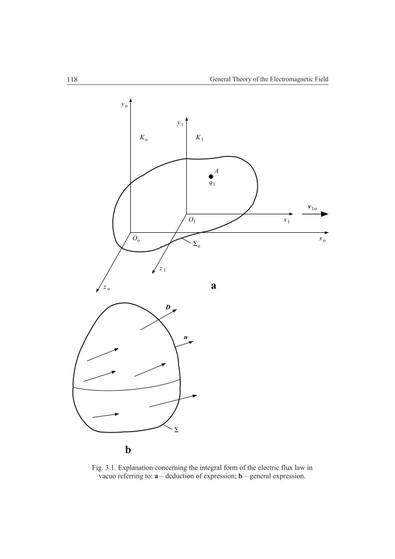
General Theory of the Electromagnetic Field118
Fig. 3.1. Explanation concerning the integral form of the electric flux law invacuo referring to: a – deduction of expression; b – general expression.
A
1z
y
1x
1y
O x
1v
o
o
oK K1
o
o
O1
oz
q1
D
n
b
a
o

The Laws of the Electromagnetic Field 119
But, in accordance with the law of electric flux in vacuo of Section 1.14, we can write:
.d 1110
1
qSE (3.3)
It results that
.d 1oo0
o
qSE (3.4)
In the case of several point-like electric charges, according to the hypothesis 2 ofSection 2.2, we can apply the principle of superposition and expression (3.4) keeps thesame form but instead of the charge 1q , the total charge
oq of the closed surface will be
introduced.The macroscopic quantities at a point, at any moment, are obtained by the
computation of the average values (mean values) of the microscopic quantities over aphysically infinitesimal volume, around the considered point and over a physicallyinfinitesimal time interval containing the considered moment.
After the calculation of the average values, the form of relation 3.3 is not modified.If instead of the point-like electric charge 1q , a distributed electric charge with the
density ov in the volume o
V is given, then, by utilizing the transformation of the
surface-integral into a volume-integral (Gauss-Ostrogradski theorem), it follows:
.ddivdd oo0ooooo0
ooo
vv
VV
v ESE(3.5 a)
Since the preceding relation is valid for any surface o , it results that:
.div oo0o vE (3.5 b)
If we renounce the index o, and consider the total charge, relations (3.4) and (3.5 a)yield:
,d0 qSE (3.6)
where q is the total charge contained by the volume bounded by the surface , and
.div 0 vE (3.7)
The expression established above remains valid for any inertial reference frame, sincethe differential operator divergence is invariant with respect to the transformation fromone inertial referential frame to another, at rest relatively to the first one.
Relations (3.6) and (3.7) represent the integral form and the local form respectively, ofthe electric flux law for empty space (i.e., in vacuo) in any inertial reference frame.
General Theory of the Electromagnetic Field120
3.1.2. The Expression of the Law of Electric Flux for Any Medium in theCase of Free (True) and Polarization Electric Charges
The expression of the law of electric flux for any medium, as previously mentioned,can be established either by the generalization of experimental results or using the resultsof the Special Theory of Relativity.
In the case of any medium, it is necessary to establish the relations between themacroscopic state quantities of the electromagnetic field. The macroscopic quantities at apoint and at a certain moment can be obtained by calculating the mean values (average)of the microscopic quantities over a physically infinitesimal volume around theconsidered point and over a physically infinitesimal time interval that contains theconsidered moment.
In the case of any medium, both free (true) electric charges and bound electric chargescan exist. If it is considered that only free electric charges exist, then, after the calculationof the mean value, the form of the relations between the various macroscopic quantitiesremains the same as for the microscopic quantities. If it is considered that both free (true)electric charges and bound electric charges exist, then, after the calculation of the meanvalue, the form of the relations between various macroscopic quantities is modified, as itwill be shown further on. The symbols and the meaning of the quantities are the onesused in Chapter 1.
It will be considered that in the inertial system of reference frame oK , in which the
vector quantity oE is expressed, there are both true (free) electric charges with the
volume density ov and polarization electric charges with the volume density opv . In
this case, after the calculation of the mean values, relation (3.4) yields:
,dd oooo0
oo
v
V
pvvSE(3.8 a)
thus:
.ddd oooooo0
oo o
vv
V
v
V
pvSE(3.8 b)
The volume density of the polarization electric charges opv in terms of the vector
quantity oP , electric polarization, in the reference frame oK , and also in any otherinertial reference frame, according to relation (1.45), is:
.div oo Ppv (3.9)
It results that:
oooooo0 dddivd
oo o
vv
V
v
V
PSE(3.10 a)
or, by transforming the first volume-integral into a surface-integral (Gauss-Ostrogradskitheorem):
The Laws of the Electromagnetic Field 121
.ddd oooooo0
oo o
v
V
vSPSE(3.10 b)
Let us denote:
.oo0o PED (3.11)
The vector quantity oD , is referred to by one of the terms: Electric displacement, electric
flux density or electric induction, and is introduced in the reference frame in which thequantities oE and oP are expressed.
Therefore, in any inertial reference frame oK , the following relations are satisfied:
,do
o
oo qSD (3.12)
,d oo
o
ovq
V
v (3.12 a)
whereo
q represents the free (true) electric charge of the interior of the surface o .
Taking into account that the two last relations are valid for any surface o and byutilizing the transformation theorem of a surface-integral into a volume-integral (Gaussand Ostrogradski theorem), relation (3.12), written in an integral form, yields thefollowing relation, in differential (local) form:
.div ooo vD (3.13)
Relations (3.12) and (3.13) represent the expressions of the integral and local form,respectively, of the law of electric flux for any medium. Relation (3.12) is also called theGauss law (theorem).
3.1.3. The General Expression of the Law of Electric Flux
The general expression of the law of electric flux, previously deduced, can beestablished as a generalization of experimental results, in the sense mentioned at thebeginning of Section 3.1.
In an inertial reference frame, in any medium, the flux of the vector electricdisplacement D through a closed surface is equal to the sum of electric true (free)charges of the inside of that surface (Fig. 3.1 b):
.d qSD (3.14)
Let us consider that the electric charge is macroscopically distributed with the volumedensity v .
By using the Gauss-Ostrogradski theorem and expression (1.11 a), relation (3.14),becomes:
General Theory of the Electromagnetic Field122
.dddiv vv
V
v
V
D (3.15)
Having in view that relation (3.15) is valid for any surface , the followingdifferential relation is obtained:
,div vD (3.16)
where the vector quantity D is the electric displacement at the considered point, and v
is the volume density of the true (free) electric charge at the same point.Relations (3.14) and (3.16) represent the integral and local form, respectively, of the
electric flux law.
3.1.4. The Electric Flux through Various Surfaces
The electric flux el through an open surface is the surface-integral of the vectors
electric induction PED 0 . It follows:
,delS
SD (3.17)
where S is any open surface bounded by the closed curve . The positive direction of
the normal to the surface S is associated to the right-handed screw rule with thetravelling direction around the curve .
For the calculation of the electric flux through a closed surface, that is the case of thelaw of electric flux, it is necessary to have in view that when calculating the surface-integral over a closed surface, the positive direction of the normal to the surface isoutward.
3.2. THE RELATION BETWEEN THE ELECTRIC DISPLACEMENT,ELECTRIC FIELD STRENGTH AND ELECTRICPOLARIZATION
We shall examine, for the case of a medium containing any substance, the relationbetween the following state quantities of the electric field: Electric displacement, electricfield strength and electric polarization.
The macroscopic state quantities of the electromagnetic field at a point and at a certainmoment are obtained by calculating the mean values of the microscopic quantities overphysically infinitesimal entities of space and time containing the considered point andmoment, respectively.
In the case of any medium, there can be both true (free) electric charges andpolarization (bound) electric charges.
The Laws of the Electromagnetic Field 123
If we consider that only free electric charge exists, then, after calculating the meanvalues, the form of relations between the values of the macroscopic quantities remain thesame as for the microscopic quantities.
But if there are free electric charges as well as polarization charges, then, aftercalculating the mean values, the form of the relations between the values of themacroscopic quantities will be modified.
In the framework of the macroscopic theory of the electromagnetic field, the vectorquantity referred to by one of the terms: Electric displacement, electric flux density or
electric induction will be introduced by the following relation:
,0 PED (3.18)
that occurred in calculations of Sub-section 3.1.2, relation (3.11).In the framework of the macroscopic theory, the vectors D and E are directly
introduced as primitive (fundamental) quantities.Relation (3.18) represents, in the framework of the macroscopic theory, the expression
of the law of relationship between the vectors: Electric displacement, electric field
strength and electric polarization.
3.3. THE LAW OF TEMPORARY ELECTRIC POLARIZATION
In the case of any isotropic medium (i.e., containing any isotropic substance), butwithout permanent electric polarization, the vector of temporary electric polarization isgenerally parallel with the electric field strength, and of the same direction. Hence:
.0 EP et (3.19)
The quantity e is termed electric susceptibility and depends on the nature of themedium, being a material quantity.
Relation (3.19) can be macroscopically established only by experimental way. Thisrelation, in the macroscopic theory of the electromagnetic field, is a material law referredto as the law of temporary electric polarization.
Practically, for variations small enough of the quantity E , the quantity e is constantwith respect to the vector quantity E for a part of the isotropic media that are calledlinear and isotropic media.
In the case of an anisotropic medium, the orientation of the vector P is not, generally,the same with that of the vector E . However, in these media it is possible to determinegenerally, three-orthogonal axes, called principal axes or eigenaxes along which theanisotropic medium behaves like an isotropic one. For these media, the law of thetemporary polarization is written in the form:
EP et 0 , (3.20)
where the tensor quantity e represents the electric susceptibility.

General Theory of the Electromagnetic Field124
For isotropic media without permanent electric polarization, the relation between thequantities electric induction, electric field strength and electric polarization (3.18)becomes:
.100 EPED et (3.21)
The following symbols are adopted:
,1 er (3.22)
.0 r (3.23)
The quantity r is called relative electric permittivity or dielectric constant of themedium and the quantity is called electric permittivity of the medium. With thesesymbols, relation (3.21) becomes:
.ED (3.24)
Taking into account the established relations that contain the quantities E and D ,certain general considerations concerning the electric field lines and electric inductionlines will be made.
Fig. 3.2. Electric hysteresis loop, the direction of travelling along the curve(upward when the electric field strength increases, downward when the
electric field strength decreases); at the middle, the branch startingfrom 0E and 0D .
O
A
A'
r
r
c c
C / m,D2
E , V / mE
D
- D
D
- D
s
s
- E
The Laws of the Electromagnetic Field 125
The line to which the vector E is tangent at any point is a line of electric field. Theline to which the vector D is tangent at any point is a line of electric displacement.
In accordance with the explanations of Sub-section 1.2.1, the lines of electric field canbe open lines that begin and end at points at which the divergence of the vector E isdifferent from zero, or can be closed lines.
As it follows from relations (3.16) and (3.24), the quantity Ediv may be differentfrom zero at points at which the density of the true electric charge is different from zeroor at points at which the permittivity varies, thus at the points at which the quantitygrad is different from zero (for example on the contact surface of two different
dielectrics, because there 0div Es ).In accordance with relation (3.16), the electric induction lines may be open lines that
begin and finish at points at which the divergence of the vector D is different from zeroor may be closed lines.
As it follows from relation (3.16), the quantity Ddiv is different from zero only atpoints at which the density of electric charge is different from zero.
Similar considerations, concerning the lines of the electric field and the lines ofelectric displacement, may be extended also for the case in which permanent electricpolarization exists. In this case, from relations (3.18), (3.24), (1.39), it follows:
.pPED (3.25)
The dependence between the quantities D and E may be linear or non-linear.Also, sometimes, the curve of D as a function of E may represent a closed curve
(Fig. 3.2) called by one of the terms: electric hysteresis loop, electric hysteresis cycle orelectric hysteresis curve. Certain characteristic points are marked on the figure.
3.4. THE LAW OF MAGNETIC FLUX
The expression of the magnetic flux can be established as a generalization of theexperimental results (i.e., in the sense mentioned at the beginning of Section 3.1) or canbe derived by using the relation established in the Special Theory of Relativity.
Further on, firstly, a derivation by using certain relations established in the SpecialTheory of Relativity will be presented.
3.4.1.The Expression of the Law of Magnetic Flux for Empty Space
Let us consider the inertial reference frames oK and 1K . The reference frame 1K is
moving with a constant velocity o1v relatively to the reference frame oK . For the sake of
simplicity, we assume xv o1o1 iv .Let us also consider one point-like electric charge q situated in empty space (i.e., in
vacuo) at a point AAA zyxA 111 ,, . We shall calculate oodiv B at any point P. We have:
.curlcurl11
divdiv ooo1o1oo2oo12ooo EvvEEvBcc
(3.26)

General Theory of the Electromagnetic Field
126
From (2.20 d) and (2.21), it follows:
,1o1o yy EE α= (3.26 a)
,1o1o zz EE α= (3.26 b)
( ) .curl 01
1
1
1o1
o
o
o
ooo =⎟⎟
⎠
⎞⎜⎜⎝
⎛∂
∂−
∂∂
α=∂
∂−
∂∂
=⋅z
Ey
Ez
Ey
E yzyzEi (3.26 c)
According to the last relation, the vector oocurl E is perpendicular to the Ox - axis. But 0curl o1o =v because the velocity is constant, and 0curl ooo1 =⋅ Ev , since the
quantities o1v and oocurl E are perpendicular to each other. Therefore, it follows:
.0div oo =B (3.27)
The left-hand side of relation (3.27) will be integrated over any closed surface Σ of the reference frame oK . Utilizing the transformation of the volume-integral into a surface integral (Gauss-Ostrogradski theorem), it follows:
.0dddiv ooooooo
=⋅= ∫∫ΣΣ
SBB vV
(3.28)
Thus, the flux of the vector oB through any closed surface is zero. In the case of several point-like electric charges, according to the assumption 2 of
Section 2.2, the principle of superposition can be applied, and for each of these charges a relation of the type (3.27) will be obtained. By summing up, side by side, these relations, it follows that the expression (3.27) remains valid. Moreover, the relation holds for any inertial reference frame (with any orientation of the three-orthogonal rectilinear system of co-ordinates), since the differential operator div is invariant relatively to the transformation of the co-ordinates when passing from one inertial frame to another, at rest, relatively to the first one.
Relations (3.27) and (3.28) represent the expressions of the local and integral form respectively, of the law of magnetic flux in empty space (i.e., in vacuo).
3.4.2. The Expression of the Law of Magnetic Flux for Any Medium
Expression (3.28), as mentioned, can be established as a generalization of experimental results (in the sense mentioned at the beginning of Section 3.1).
In the case of any medium (i.e., containing any type of substance), the aim is to establish the relations between the macroscopic state quantities of the electromagnetic field.
The macroscopic quantities at a point and at a certain moment are obtained by the calculation of the mean values of microscopic quantities over a physically infinitesimal volume, around the considered point and over a physically infinitesimal time interval containing the considered moment.

The Laws of the Electromagnetic Field 127
Fig. 3.3. Explanation referring tothe law of magnetic flux.
Fig. 3.4. Two open surfaces that arebounded by the same closed curve .
In the case in which electric charges do not directly occur in relations, then, after thecalculation of average values, the form of relations between the macroscopic quantitiesremains the same as for the microscopic quantities. For this reason, relations (3.27) and(3.28) remain also valid for any medium.
3.4.3. The General Expression of the Law of Magnetic Flux(for Any Medium)
The general expression of the law of magnetic flux derived previously, as mentioned,can be established as a generalization of experimental results (in the sense mentioned atthe beginning of Section 3.1).
In an inertial reference frame, in any medium, the flux of the vector magnetic inductionB through a closed surface is zero (Fig. 3.3):
.0d SB (3.29)
Utilizing the Gauss-Ostrogradski theorem, relation (3.29) becomes:
.0ddiv v
V
B (3.30)
Taking into account that relation (3.30) remains valid for any closed surface , thefollowing relation in differential form will be obtained:
.0div B (3.31)
n
B
n
n
S
S
1
2
2
1

General Theory of the Electromagnetic Field
128
Expressions (3.29) and (3.31) represent the integral form and local form, respectively, of the law of magnetic flux for any medium. The vector quantity B is introduced as shown in Section 2.5.
By comparing the local form of the law of electric flux with the local form of the law of magnetic flux, it results that the field of vectors B has no sources (because 0div =B ). Therefore, the following statement is equivalent: The existence of magnetic forces, having the direction and the orientation of the vector B is not possible.
Certain investigators, for instance Dirac, in the year 1948 [18, p. 43] supposed that true magnetic charges referred to as magnetic monopoles, could exist or could be produced in accelerators of high energies.
If magnetic monopoles existed, then the lines of magnetic field would diverge from the magnetic monopoles like the lines of electric field diverge from the electric charges. For a system of magnetic monopoles, the divergence of the magnetic induction would not be zero, but equal to the volume density of the magnetic charge.
Up to now, the existence of magnetic monopoles, despite many investigations made during the recent years, has not been proved. Even if the existence of magnetic monopoles were established, the equations of the electromagnetic field would have to be modified only in quite special cases, in order to take into account the presence of magnetic monopoles.
It follows that it is justified to assume that true magnetic charges have not to be taken into consideration, and the divergence of the vector magnetic induction is zero.
In a vector field which has the divergence zero, the lines of field are always closed. Thus the lines of magnetic induction are always closed lines because in the magnetic field there are no sources (magnetic charges).
3.4.4. The Magnetic Flux through Various Surfaces
The magnetic flux Ψ through an open surface is the surface integral of the vector magnetic induction:
,d∫Γ
⋅=ΨS
SB (3.32)
where ΓS is a simply connected open surface bounded by the closed curve Γ . The positive direction of the normal to the surface ΓS is associated according to the right-handed screw rule with the travelling sense along the curve Γ .
The magnetic flux through two open simply connected surfaces bounded by the same closed curve Γ is the same. Indeed, if we consider two surfaces
1ΓS and 2ΓS , bounded
by the same curve, their union forms a closed surface. In this case, by virtue of the law of magnetic flux, it follows (Fig. 3.4):
,021=Ψ−Ψ
ΓΓ SS (3.32 a)
and hence (according to the explanation below), it follows:
.21 ΓΓ
Ψ=Ψ SS (3.33)

The Laws of the Electromagnetic Field 129
When applying the law of magnetic flux, it is necessary to take into account that at thecalculation of a surface-integral over a closed surface, the positive direction of the normalto the surface is outward. Consequently, in the case of the preceding example, the positivedirection of the normal to one of the open surfaces, in accordance with the chosen senseof travelling the bounding curve, will be opposite with respect to the positive direction ofthe normal to the closed surface, resulted from the union of the two open surfaces.
3.4.5. The Magnetic Flux-Turn. The Magnetic Flux-Linkage.Magnetic Vector Potential.
In the case in which the curve that bounds the surface S through which themagnetic flux has to be calculated is taken along the conductor (wire) of a coil having wturns (Fig. 3.5), the notions of magnetic flux-turn and magnetic flux-linkage have to beintroduced (defined). It is to be noted that the number of turns of a coil or generally ofany winding can be denoted by w as well as by N, the last being utilized in severalstandards. However, we shall prefer the former symbol, because the latter has also othermeanings in certain applications widely utilized.
Fig. 3.5 shows the coil conductor, two lines of magnetic induction, a helical surface(hatched) bounded by the coil contour and also the electric tension between the twopoints M and N of the coil.
The magnetic flux-turn is the magnetic flux that crosses the portion of the helicalsurface bounded by a single turn of the coil, according to relation:
.d
wS
SB(3.34)
The magnetic flux through the whole surface is calculated taking into account that aline of magnetic field intersects several times the surface.
The magnetic flux-linkage, also called total magnetic flux, is the magnetic flux thatcrosses the helical surface bounded by all the turns of the coil, according to relation:
.dS
SB (3.35)
The last two relations yield:
,w (3.36)
because the same line of magnetic field intersects w times the helical surface that isbounded by all the turns of the coil. If the magnetic flux-turn has not the same value forall the turns, then a mean value of the magnetic flux turn, also called average magnetic
flux-turn, will be used.According to relation (3.31), the divergence of the vector B is always zero.
Consequently, it is possible to express the vector B as follows:
,curl AB (3.37)
where A denotes the quantity called magnetic vector potential. Since the divergence of acurl is always zero, several vectors A can give the same vector magnetic induction B .

General Theory of the Electromagnetic Field130
Fig. 3.5. Explanation to thecalculation of magnetic fluxes:
flux-turn and flux-linkage.
For example, the vectors ByiA and BxjA give the same vector BkB .This circumstance is of no interest, for only the value of B is important in this case.
By employing the last relation, the magnetic flux through an open surface, aspreviously, can be expressed in the form:
,dcurldSS
SASB (3.38)
that, by using the Stokes theorem, becomes:
.dd lASB
S(3.39)
Therefore, the magnetic flux through a simply connected open surface bounded by aclosed curve can be calculated by a line-integral along that curve. By using this
u MN
M
N
+
-
B
-
S
n
n
n

The Laws of the Electromagnetic Field
131
expression, the conclusions obtained above concerning the flux through surfaces related to some curves result directly.
3.5. THE LAW OF ELECTROMAGNETIC INDUCTION FOR MEDIA AT REST
The expression of the law of electromagnetic induction may be established by a generalization of experimental results (i.e., in the sense mentioned at the beginning of Section 3.1) or deduced by utilizing certain relations established in the Special Theory of Relativity. We shall use both manners beginning with the second one.
3.5.1. The Expression of the Law of Electromagnetic Induction for Empty Medium at Rest
Let oK and 1K be the two inertial reference frames. The reference frame 1K is moving at a constant velocity o1v relatively to the reference frame oK .
We shall consider a point-like charge 1q , situated in empty space (i.e., in vacuo) at any point ( )1A1A1A ,, zyxA fixed to the reference frame 1K , and we shall calculate
oocurl E at the point ( )ooo ,, zyxP . It follows:
.curl
ooo
ooooo
zyx EEEzyx ∂∂
∂∂
∂∂
=
kji
E (3.40)
The component along the oo xO - axis is:
,o
o
o
oz
Ey
E yz∂
∂−
∂∂ (3.40 a)
and by using relations (2.21), (2.18 b, c) and (2.17), we obtain:
( )( ) ( ),34
511o1oo1
0
1
o
o −−−αεπ
=∂∂ −rzzyy
qy
EAA
z (3.41 a)
( )( ) ( ).34
511o1oo1
0
1
o
o −−−αεπ
=∂
∂ −ryyzzq
zE
AAy (3.41 b)
By replacing relations (3.41 a, b) into expression (3.40 a), it follows:
.0o
o
o
o =∂
∂−
∂∂
zE
yE yz (3.42 a)
General Theory of the Electromagnetic Field132
Analogously, it follows that the components along the axes oo yO and oo zO are:
,34
51
2o1
2o11o1oo1oo1
0
1
o
o
o
o rzzxtvxq
x
E
z
EAAx
zx(3.42 b)
,34
51
2o1
2o11o1oo1oo1
0
1
o
o
o
oryyxtvx
q
y
E
x
EAAx
xy(3.42 c)
because
.1
111
;
;1
1
2o1
2o12
o1
2o1
o1o1
2o1
2o1
c
v
(3.42 d)
(3.42 e)
(3.42 f)
Now, we calculate the vector quantity:
.o
o
o
o
o
o
o
o
t
B
t
B
t
B
t
zyx kjiB
(3.43)
According to relation (2.26) and taking into account that 200
1
c, the vector
quantity oB is:
.11
001
1o1o121o1o12
ooo
o12o yxzx
zyx
x Ec
Ec
EEE
cvkvjv
kji
B (3.44)
After the calculation of derivatives, we obtain the components:
,0o
o
t
B x(3.45 a)
,4
13 5
11o1oo1oo10
12o1
2o12
o
orzzxtvx
qv
ct
BAAx
y(3.45 b)
.4
13 5
11o1oo1oo10
12o1
2o12
o
o ryyxtvxq
vct
BAAx
z(3.45 c)
It follows that:

The Laws of the Electromagnetic Field 133
,0o
o
o
o
o
o
t
B
z
E
y
E xyz (3.46 a)
,o
o
o
o
o
o
t
B
x
E
z
E yzx (3.46 b)
.o
o
o
o
o
o
t
B
y
E
x
Ezxy
(3.46 c)
Thus:
.curlo
ooo
t
BE (3.47)
We shall integrate both sides of the last equation (3.47) over any simply connectedopen surface
oS bounded by the closed curve o , both at rest relatively to the reference
frame oK . By expressing this operation, it follows:
,ddcurl oo
oooo
oo
SB
SE
SS
t (3.48)
and by transforming the surface-integral into a line-integral (Stokes theorem), it follows:
.dd oo
ooo
oo
SB
lE
S
t (3.49)
In the case in which there are several point-like electric charges, according to theassumption 2 of Section 2.2, the principle of superposition may be applied and expression(3.49) remains valid also in this case. Expression (3.49) remains valid for each inertialsystem, since the differential operator curl is invariant with respect to the transformationfrom one reference frame to another one if the latter is at rest relatively to the former one.
Relations (3.47) and (3.49) represent the local and integral forms, respectively, of thelaw of electromagnetic induction for empty space, and reference frame at rest.
3.5.2. The Expression of the Law of Electromagnetic Inductionfor Any Medium at Rest
In the case of any medium (i.e., containing any substance, whatever it would be), it isnecessary to establish the relations between the macroscopic state quantities of theelectromagnetic field.
The macroscopic quantities at a point, at a certain instant, are obtained by the averageof the microscopic quantities over a physically infinitesimal volume around theconsidered point, and over a physically infinitesimal time interval that contains theconsidered instant (time). As in Sub-section 3.4.2, the law keeps its previous form.
General Theory of the Electromagnetic Field134
3.5.3. The General Expression of the Law of Electromagnetic Inductionfor Media at Rest
The general expression of the law of electromagnetic induction, previously derived,can be established by the generalization of experimental results (in the sense mentioned atthe beginning of Section 3.4).
In an inertial reference frame, in any medium, the following relation exists betweenthe vector quantities E and B :
,dd
S
tS
BlE (3.50)
where S is a simply connected open surface bounded by the closed curve , both at restrelatively to the considered inertial reference frame. The curve may represent anycontour in particular it can even be the contour of an electric circuit. The last situation isof great interest in applications.
The positive direction of the normal to the surface S is associated according to theright-handed screw rule with the travelling sense of the curve (Fig. 3.6).
Relation (3.50) can also be written in the form:
,d magilE (3.51)
where the quantity magi is called, according to the work [3, p. 259], intensity of magnetic
current.By using the Stokes theorem, relation (3.50) becomes:
.ddcurl SB
SE
SS
t (3.52)
Taking into account that the last relation holds for any surface S , the followingrelation in differential (local) form is obtained:
.curlt
BE (3.53)
Relation (3.53) may also be written in the form [3, p. 367]:
,curl magJE (3.54)
where the quantity magJ is called [3, p. 260] magnetic current density.
Relations (3.50) and (3.53) represent the expressions of the integral form and local
form, respectively, of the law of electromagnetic induction for any medium at rest.The vector quantities E and B can be introduced as shown in Section 2.5.

The Laws of the Electromagnetic Field 135
Fig. 3.6. Explanation to thelaw of electromagnetic
induction.
3.5.4. The Concise Integral Form of the Expression of the Law ofElectromagnetic Induction for Media at Rest. Faraday Law.
The left-hand side of relation (3.50) represents the induced electromotive force (by thesolenoidal component of the electric field) along the curve :
.d lEeu (3.55)
It is to be remarked that, in this case, the electric field strength E contains only theCoulombian and induced component, but not the impressed component, hence:
.il EEE (3.55 a)
The integral of the Coulombian component along the closed curve is zero, since itderives from a potential.
Also, it can be seen that the right hand side of relation (3.50) may be written in thefollowing form (since the surface S is at rest):
,d
dd
S
Stt
SB
(3.56)
where
S
S ,d SB (3.56 a)
represents the magnetic flux through any open surface S .It follows:
,d
d
tu
S
e (3.57)
B
E
E
n
S
B
B
General Theory of the Electromagnetic Field136
that represents another manner of writing the integral form of the law of electromagneticinduction for media at rest. This law is also called the Faraday law.
The phenomenon of producing an electromotive force along a closed curve Γ by thevariation with time of the magnetic flux which links that curve is called electromagneticinduction. The electromotive force produced in this way is called induced electromotiveforce, and the magnetic flux that produces the electromotive force is termed inductivemagnetic flux.
The variation with time of the magnetic flux through any surface bounded by thecurve Γ can have two causes:
a. Variation with time of the local magnetic induction (for instance due to thevariation with time of the electric current carried by the circuits which produce themagnetic field);
b. Motion of the contour Γ .The electromagnetic induction is referred to in the first case as induction by
transformation and, in the second case, induction by motion; in particular it can beinduction by rotation (i.e., rotation without translation) and induction by deformation.
The inductive magnetic flux can be produced by a permanent magnet or by electriccurrents. The inductive magnetic flux can be produced even by the electric current (if itexists) flowing along the circuit for the contour of which the electromotive force has to becalculated, and also by the currents flowing along other circuits. Correspondingly, theelectromagnetic induction is referred to as self-induction and mutual induction,respectively.
3.6. THE LAW OF MAGNETIC CIRCUIT (MAGNETIC CIRCUITALLAW) FOR MEDIA AT REST
The law of magnetic circuit also called magnetic circuital law can be established bythe generalization of certain experimental results (in the sense mentioned at the beginningof Section 3.1) or derived by employing certain relations established in the SpecialTheory of Relativity. We shall use both manners beginning with the second one.
3.6.1. The Expression of the Law of Magnetic Circuit for Empty Mediumat Rest
Let oK and 1K be two inertial reference frames. The reference frame 1K is movingwith the constant velocity o1v with respect to the reference frame oK . Let 1q be a point-like electric charge fixed in empty space at any point ( )AAA zyxA 111 ,, .
We shall calculate the vector quantity oocurl B at a point ( )ooo ,, zyxP . Taking intoaccount relation (2.26), we can write:
( ) ( ).curlcurlcurl oo1o00o0o10ooo EvEvB ×με=ε×μ= (3.58)
By using an expression of the Vector Calculus, namely:
( ) ( ) ( ) ,divdivcurl ababbababa −∇⋅+∇⋅−=× (3.58 a)

The Laws of the Electromagnetic Field 137
it follows:
.
divdivcurl
o1oo00
ooo100o1oo00ooo100oo
vE
EvvEEvB(3.59)
But 0div o1ov and 0o1oo vE because the velocity o1v is constant. Hence, itfollows:
.divcurl ooo100ooo100oo EvEvB (3.60)
From the known relation of Vector Calculus, it follows:
,o
oo1ooo1
xv x
EEv (3.61)
where we have taken into account that xv o1o1 iv .Now, we calculate the following vector quantity:
.o
o
o
o
o
o
o
o
x
E
x
E
x
E
x
zyx kjiE
(3.62)
Since we have supposed that there is a single point-like electric charge 1q , it results that:
,4 3
1
1oo1oo1
0
11o
r
xtvxqEE Ax
xx (3.63 a)
,4 3
1
1o
0
1o11o1o
r
yyqEE A
yy (3.63 b)
.4 3
1
1o
0
1o11o1o
r
zzqEE A
zz (3.63 c)
Taking into account all these relations (3. 63 a, b, c) in the general case of any systemof electric charges, it results that:
.o
o
o
oo1oo1
txv x
EEEv (3.64)
It follows:
.divcurlo
o00ooo100oo
t
EEvB (3.65)
In the case in which there are several point-like charges, according to the assumptionsof Section 2.2, the principle of superposition can be applied, and the last relation keeps itsform.
The macroscopic quantities at a point, at a certain moment, are obtained by theaverage of the microscopic quantities over a physically infinitesimal volume, around the

General Theory of the Electromagnetic Field138
considered point, and over a physically infinitesimal time interval including theconsidered moment (time). After the calculation of the average (mean) values, the form ofrelation (3.65) remains unchanged.
Let us consider the free (true) electric charge continuously distributed in empty space,with the volume density ov , in the interior of the surface o . In accordance with the lawof electric flux, it can be written:
.div ooo0 vE (3.65 a)
Consequently, it follows:
o
o00o1o0oocurl
tv
EvB (3.65 b)
or
.curlo
o0o1o
0
oo
tv
Ev
B(3.66)
If we denote:
,o1oo vJ ve (3.67)
the density of the current constituted by the electric charges in motion, the last relationyields:
.curlo
o0o
0
oo
te
EJ
B(3.68)
We shall integrate both sides of relation (3.68) over any open surface o
S bounded by
the closed curve o , both in the reference frame oK . It follows:
.dddcurl
oo
o
oo
o0ooo
0
oo
SS
e
S
tS
ESJS
B
(3.69)
By using the transformation of the surface-integral into a line-integral (Stokestheorem), it follows:
.ddd
ooo
oo
o0ooo
0
o
SS
et
SE
SJlB
(3.70)
Expression (3.70) remains valid for any inertial reference frame, for the differentialoperator curl is invariant with respect to the transformation from one inertial referenceframe to another, at rest relatively to the previous one.
Relations (3.68) and (3.70) represent the expressions of the local form and integral
form, respectively, of the law of magnetic circuit for empty space (i.e., in vacuo), andreference frame at rest.

The Laws of the Electromagnetic Field 139
3.6.2. The General Expression of the Law of Magnetic Circuitfor Empty Space
The general expression (3.70), previously derived, can also be established as ageneralization of experimental results (in the sense mentioned at the beginning of Section3.1).
In an inertial reference frame, between the vector quantities: Magnetic induction B ,density of the resultant electric current (produced by the electric charges in motion) eJ ,
and product of the permittivity of vacuum by the electric field strength E0 , thefollowing relation exists in empty space:
,ddd 0
0S
S
et
SE
SJlB
(3.71)
where S is a simply connected open surface, bounded by the closed curve , both atrest with respect to the considered inertial reference frame. The positive direction of thenormal to the surface S is associated, according to the right-handed screw rule, with the
travelling sense along the curve . The quantity 0 is a universal constant referring tovacuum, and termed magnetic constant or permeability of vacuum. In the SI system ofunits, it has, as mentioned in Section 2.4, the value:
.m/H104 70 (3.72)
By using the Stokes theorem, relation (3.71) becomes:
.dddcurl 0
0S
S
e
S
tS
ESJS
B
(3.73)
Taking into account that the last relation holds for any surface S , the followingrelation, in local (differential) form, is obtained:
.curl 0
0 te
EJ
B(3.74)
Relations (3.71) and (3.74) represent the expressions of the integral form and localform, respectively, of the law of magnetic circuit for empty space, and frame at rest.
The vector quantities B and E can be introduced as shown in Section 2.5.
3.6.3. The Expressions of the Law of Magnetic Circuit and MagneticField Strength, for Any Medium at Rest, in the Case of all Types ofElectric Charges and Currents
The expression of the law of magnetic circuit for any medium (i.e., containingwhatever substance) at rest can be obtained by the generalization of certain experimentalresults (in the sense mentioned at the beginning of Section 3.1).

General Theory of the Electromagnetic Field140
In the case of any medium, it is necessary to establish relations between themacroscopic state quantities of the electromagnetic field.
The macroscopic quantities at a point, at a certain moment, are obtained by calculatingthe average of the microscopic quantities over a physically infinitesimal volume, aroundthe considered point, and over a physically infinitesimal time interval including theconsidered moment (time). In the case of a medium, in which only free charges can exist,after the calculation of the average (mean) values, the form of the relations between thevarious macroscopic quantities will not be modified (they will remain as in the case ofmicroscopic values). If there are free electric charges, polarization electric charges, andAmperian electric currents, then, after the calculation of the average (mean) values, theform of the relations between the various macroscopic quantities will be modified.
The symbols and their meaning are the same as in Section 1.10.The electric current density eJ (of relation (3.67), but without index o) in the case of
macroscopic quantities can be expressed as the sum of three components: the density of
electric conduction currents J , the density of Amperian electric currents aJ , and the
density of polarization electric currents PJ . Consequently, the following relation isobtained:
.Pae JJJJ (3.75)
By replacing the quantities of relation (3.75) into relation (3.74), it results that:
.curl 0
0 tPa
EJJJ
B(3.76)
If we integrate both sides of relation (3.76) over any open surface bounded by a closedcurve , and we utilize the transformation theorem of a surface-integral into a line-integral (Stokes theorem), the following relation between the macroscopic quantities isobtained:
.ddddd 0
0S
S
P
S
a
St
SE
SJSJSJlB
(3.77)
In the right-hand side, the second term represents the intensity of the Amperianelectric current given by relation (1.90), and the third term represents the intensity of thepolarization electric current given by relation (1.75). By performing the correspondingsubstitutions and grouping the terms, it follows:
.ddd1
000
SS
tSPESJlMB (3.78)
Taking into account relation (3.18), relation (3.78) can be written:
,ddd
SS
tS
DSJlH (3.79)

The Laws of the Electromagnetic Field 141
where we have denoted:
MBH0
1(3.80 a)
or
.11
00jMBH (3.80 b)
The vector quantity H , defined by each of relation (3.80 a, b), is called magnetic field
strength or magnetic field intensity and is a function of point or, in other words, itrepresents a vector field. The lines of the vector field H , called lines of magnetic field
strength, are the lines to which the vector H is tangent at each point. Analogously, thelines of the vector field B , called lines of magnetic induction or lines of magnetic field,
are the lines to which the vector B is tangent at each point.A tube of magnetic flux is termed each surface in the magnetic field formed by the
totality of lines of magnetic induction passing through the points of a simple closed curve.In the SI system of units, the unit of measure of the electric field strength is the
ampere per metre, symbol m/A . A definition of this unit will be given in Section 3.15.Relation (3.79) can also be written in the form:
,dd
ddd SDSJlH
SSt (3.81)
because the position of the differential operator is indifferent in the case in which thederivative does not concern the variable with respect to which the integral is to becalculated, and the surface S is considered at rest.
By using the Stokes theorem, relation (3.79) becomes:
.dddcurl
SSS
tS
DSJSH (3.82)
Having in view that the previous relation is valid for any surface S , the followingrelation in local (differential) form can be obtained:
.curlt
DJH (3.83)
Relations (3.81) and (3.83) represent the expressions of the integral form and local
form, respectively, of the law of magnetic circuit for any medium at rest, in the case in
which, there are free electric charges, polarization electric charges and Amperian
electric currents.A detailed analysis of the introduction of the physical quantities E, D, H, B can be
found in papers [55], [56].
General Theory of the Electromagnetic Field142
3.6.4. The General Expression of the Law of Magnetic Circuit for AnyMedium at Rest
The general expression of the law of magnetic circuit for media at rest, derivedpreviously, can be established by the generalization of certain experimental results.
In an inertial reference frame, and in any medium, the following relation existsbetween the vector quantities H , J , D :
,ddd
SS
tS
DSJlH (3.84)
where S is any simply connected open surface bounded by the closed curve , both atrest relatively to the reference frame. The positive direction of the normal to the surfaceS is associated with the travelling sense along the curve by the right-handed screwrule.
If, in the considered space, there are bodies charged with electricity with the volumedensity conv , in motion at any velocity rv relatively to the reference system, then, in theright-hand side of relation (3.84), another term occurs. Indeed, the motion of bodiescharged with electricity represents a supplementary electric current called convection
electric current. In this general case, expression (3.84) becomes:
,dddd conv
SSS
tS
DSJSJlH (3.84 a)
where the quantity rvJ convconv is the density of the convection electric current.Relation (3.84 a) may also be written in the form:
,d lilH (3.85)
where the quantity li represents the intensity of the electric current in the large sense.
Having in view that relations (3.84) and (3.84 a) hold for any surface S , and usingthe Stokes theorem, the following two relations, in differential (local) form, are obtained:
,0,curl convJD
JHt
(3.86)
.curl convt
DJJH (3.86 a)
Relations (3.86) and (3.86 a) can also be written in the form:
,curl lJH (3.87)
,convt
l
DJJJ (3.87 a)

The Laws of the Electromagnetic Field 143
where the quantity lJ represents the density of the electric current in the large sense.Relations (3.84), (3.84 a) and (3.86), (3.86 a) represent the expressions of the integral
form and local form, respectively, of the law of magnetic circuit, for any media at rest.The vector quantities H and D are defined by relations (3.80 b) and (3.18),
respectively.In the right-hand side of relation (3.84 a) the three terms have the following meaning,
respectively: intensity of the conduction electric current, intensity of the convection
electric current, and intensity of the displacement electric current. The intensity of thedisplacement electric current is the sum of the intensity of the displacement electriccurrent in vacuo and the intensity of the polarization electric current. The sum of theterms of the right-hand side of relation (3.84 a) is referred to as intensity of the electric
current in the large sense.
3.6.5. Conditions (Regimes) of the Electromagnetic Field.Law of Magnetic Circuit in Quasi-stationary Condition.Ampère Law (Theorem).
The electromagnetic field can be in one of the following conditions also calledregimes: Static condition, Stationary condition, Non-stationary condition, Quasi-stationary condition.
Static condition is the regime in which no macroscopic quantity varies with time andno electric current exists.
Stationary condition is the regime in which no macroscopic state quantity varies withtime and electric current exists but does not vary with time.
Non-stationary condition is the regime in which the macroscopic state quantities varywith time.
Quasi-stationary condition is the regime in which the macroscopic quantities varywith time but their variation is relatively slow, implying the following consequences. The
value of the quantityt
Dmay be neglected with respect to the quantity J , at any point
of a conducting medium or a medium in which a convection electric current exists; butthe derivatives with respect to time of the other state quantities of the electromagneticfield cannot be neglected. One of the practical results of these remarks results in the factthat in an electric circuit in quasi-stationary condition, the intensity of the electric currentis assumed to have the same value at any cross-section of the circuit wire. The higher thespeed of variation of the state quantities (e.g., magnetic induction), the farther from theprevious assumption the circuit will be.
In quasi-stationary condition, the expressions of the integral form and local form,respectively, of the law of magnetic circuit (without including the convection current)become:
,ddS
SJlH (3.88)
,curl JH (3.89)
General Theory of the Electromagnetic Field144
and are referred to as the integral form and the local form, respectively, of the Ampère
theorem or of the Ampère circuital law.Expression (3.88) may be obtained by employing the Biot-Savart-Laplace formula
(2.47), and (2.48), if it is previously known. For this purpose, formula (2.48) will beapplied for a closed curve , and the expression of the solid angle, and certain vectortransformations are to be used [23, p. 120].
3.6.6. The Components of the Magnetic Field Strength. MagneticTension. Magnetomotive Force.
The magnetic field strength has generally two components: a potential (non-curl,
irrotational) component pH and a curl (rotational, solenoidal) component rH . Hence:
.rp HHH (3.90)
Generally, in a field of vectors, the line-integral of the field vector along a curve canbe referred to as tension; this tension is also introduced in the case of magnetic field. Thedefinitions, in the case of the magnetic field, are analogous to those introduced for theelectric field in Section 1.8.
The line-integral of the magnetic field strength along a curve is called magnetic
tension and is given by the relation:
.d
AB
AB
C
Cmu lH (3.91)
If in relation (3.91), instead of the magnetic field strength H , only the curl component
rH of the magnetic field strength is introduced, the magnetomotive tension calculated byemploying a line-integral (along an open curve) is termed magnetomotive force
(abbreviation m.m.f.) along that curve, and is obtained by the relation:
.d
AB
AB
C
rCmmu lH (3.92)
If the line-integrals (3.91) and (3.92) along a closed curve are considered, the obtainedexpression is called magnetomotive force, also termed magnetomotive tension, along thatcurve. The magnetomotive force obtained by integrating the magnetic field strength H
along a closed curve coincides with the integral of the curl component of the magneticfield strength, because the line-integral of the potential component of the magnetic fieldstrength is zero along a closed curve.
All the definitions of magnetic tensions refer to any medium, regardless of its state.
3.6.7. The Concise Integral Form of the Law of Magnetic Circuit forMedia at Rest
The left-hand side of relation (3.84) represents the magnetomotive force along theclosed curve :

The Laws of the Electromagnetic Field 145
.d lHmmu (3.93)
It is to be remarked that the magnetomotive force is determined only by the curl(rotational) component of the magnetic field strength.
The first term of the right-hand side of relation (3.84 a), i.e., the flux of the vector ofthe conduction electric current density through the surface S , bounded by the closedcurve , is called current-linkage and is determined by the conduction electric currentthat crosses the surface S . The current-linkage is given by the relation:
.dS
SJ (3.94)
Let us consider a coil with w turns carrying an electric current. We shall adopt a curvelinking the coil as it can be seen in Fig. 3.7.
In this case, a simply connected open surface S , bounded by the curve , is crossedat w places by the conductor carrying the current i . At the other points of the surface,the density of the conduction electric current is zero. It follows:
.iw (3.95)
Analogously, for the coils of Fig. 3.8, the following result is obtained:
.2211 iwiw (3.95 a)
In the case of coils, the current linkage is also expressed by the denomination ampere-
turns.The last term of the right-hand side of relations (3.84) and (3.84 a), i.e., the flux of the
vectort
Dthrough the surface S is called displacement electric current. If the
considered condition is quasi-stationary, it will be disregarded.It can be remarked that the expression of the displacement electric current of the right-
hand side in relations (3.84) and (3.84 a) can be written:
,dd
dd SDS
D
SS
tt (3.96)
because the order of the differential and integral operators is indifferent, since thederivation does not refer to the variable of integration, and the surface S is at rest.
But, the surface S being at rest, it results that:
,d
dd
d
del S
Stt
SD (3.97)

General Theory of the Electromagnetic Field146
Fig. 3.7. Coil linked by a curve of integration – curve .
Fig. 3.8. Two coils disposed on aclosed core made of ferromagnetic
material and the curve ofintegration.
where
SD delS
S (3.97 a)
represents the electric flux through the open surface S .Hence:
Smmt
iu elconv d
d(3.98)
that represents another way of writing the integral form of the law of magnetic circuit(magnetic circuital law) for media at rest.
Remark. It can be added that a coil constituted by a wire, wound on a cylinder, in the
i
S
w
u u
i i
w w1 1
1 2
2 2

The Laws of the Electromagnetic Field 147
3.6.8. Adoption of the Curves and Surfaces That Occur in theExpressions of the Laws of Electromagnetic Induction,and Magnetic Circuit
All differential operations t
div,curl, are performed in the fixed reference system,
i.e., assumed at rest.The curve and the surface S are taken in the fixed reference frame, but may also
be taken in the moving reference frame. Concerning this circumstance, it is to be notedthat, in both cases, the curve and the surface S occur only by the elements ld and
Sd at any moment. The motion occurs by the velocity and by the determination of thevarious quantities in the two reference frames.
In most of cases, the laws are written for determining the quantities and relations inthe moving reference frame with respect to the fixed one.
3.7. THE RELATIONSHIP BETWEEN MAGNETIC INDUCTION,MAGNETIC FIELD STRENGTH AND MAGNETICPOLARIZATION
In the case of a medium containing any substance, it is important to know the relationbetween the macroscopic state quantities of the magnetic field, i.e., magnetic induction,magnetic field strength and magnetization or magnetic polarization.
The macroscopic state quantities of the electromagnetic field at a point, at a givenmoment, are obtained by calculating the average value of the microscopic quantities overthe physically infinitesimal of volume and of time interval, respectively, containing thepoint and time under consideration.
From relations (3.80 a, b), it follows that:
.00 jMHMHB (3.99)
In the framework of the macroscopic theory, this formula constitutes the expression of
the law of relationship between the vectors: Magnetic induction, magnetic field strength
and magnetization (or magnetic polarization). In the framework of the macroscopictheory, the quantities above and their relationship have to be introduced as primitive(fundamental) quantities and law, respectively.
3.8. THE LAW OF TEMPORARY MAGNETIZATION
In the case of any isotropic medium (hence, containing any substance), but withoutpermanent magnetization (or magnetic polarization), the temporary magnetization vector(temporary magnetic polarization vector) is parallel with the magnetic field strengthvector and of the same direction, as follows:
General Theory of the Electromagnetic Field148
,HM mt (3.100 a)
.0 HM mjt (3.100 b)
The quantity m is called magnetic susceptibility and is depending on the nature ofthe medium, hence a material quantity.
In the framework of the macroscopic theory, relation (3.100 a) can be determined onlyexperimentally. In the macroscopic theory of electromagnetic field, this relation is amaterial law, also termed constitutive law, referred to as the law of temporary
magnetization, or the law of temporary magnetic polarization, as the reference concernsrelation (3.100 a) or (3.100 b), respectively.
In fact, for variations slow enough of the quantity H , the quantity m is constantwith respect to the vector quantity H for certain isotropic media called isotropic andlinear media.
In the case of anisotropic media, the orientation of the vector M is not, generally, thesame as that of the vector H . However, in these media, it is possible to determine,generally, three-orthogonal axes, termed principal axes or eigenaxes, along which theanisotropic medium behaves like an isotropic medium. For these media, the law oftemporary magnetization (or of the temporary magnetic polarization, respectively) iswritten in one of the following forms:
,HM mt (3.101 a)
,0 HM mjt (3.101 b)
where the quantity m represents the tensor of the magnetic susceptibility.For isotropic media without permanent magnetic polarization, the expression of the
relationship between the magnetic induction, the magnetic field strength andmagnetization (or magnetic polarization, respectively) (3.99) becomes:
,100 HMHB mt (3.102 a)
.100 HMHB mjt (3.102 b)
The following symbols are adopted:
,1 mr (3.103)
.0 r (3.104)
The quantity r is called relative magnetic permeability of the medium, and the
quantity is the magnetic permeability of the medium.With the adopted symbols, relations (3.102 a, b) become:
.HB (3.105)
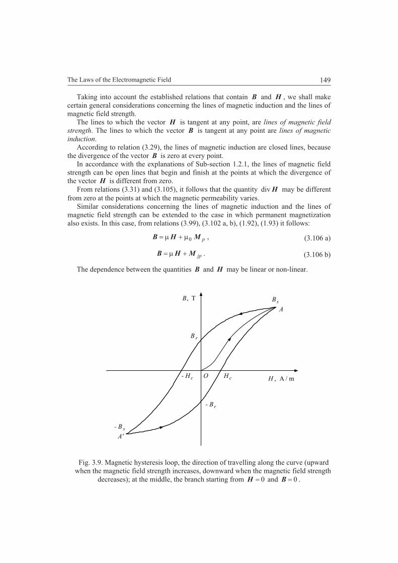
The Laws of the Electromagnetic Field 149
Taking into account the established relations that contain B and H , we shall makecertain general considerations concerning the lines of magnetic induction and the lines ofmagnetic field strength.
The lines to which the vector H is tangent at any point, are lines of magnetic field
strength. The lines to which the vector B is tangent at any point are lines of magnetic
induction.According to relation (3.29), the lines of magnetic induction are closed lines, because
the divergence of the vector B is zero at every point.In accordance with the explanations of Sub-section 1.2.1, the lines of magnetic field
strength can be open lines that begin and finish at the points at which the divergence ofthe vector H is different from zero.
From relations (3.31) and (3.105), it follows that the quantity Hdiv may be differentfrom zero at the points at which the magnetic permeability varies.
Similar considerations concerning the lines of magnetic induction and the lines ofmagnetic field strength can be extended to the case in which permanent magnetizationalso exists. In this case, from relations (3.99), (3.102 a, b), (1.92), (1.93) it follows:
,0 pMHB (3.106 a)
.jpMHB (3.106 b)
The dependence between the quantities B and H may be linear or non-linear.
Fig. 3.9. Magnetic hysteresis loop, the direction of travelling along the curve (upwardwhen the magnetic field strength increases, downward when the magnetic field strength
decreases); at the middle, the branch starting from 0H and 0B .
T
O H
A
A'
B
A / m
- B
H ,
B,
- B s
r
r
c c
sB
- H
General Theory of the Electromagnetic Field150
Also, sometimes, the curve of B as a function of H may represent a closed curve(Fig. 3.9) referred to by one of the terms: hysteresis loop, hysteresis cycle, hysteresis
curve. Certain characteristic points are marked on the curve.
3.9. DERIVATION OF THE FUNDAMENTAL EQUATIONS OF THEELECTROMAGNETIC FIELD THEORY IN THE GENERALCASE. MAXWELL EQUATIONS.
In the preceding Sections, we have derived the fundamental laws of the theory of theelectromagnetic field in the case in which the velocities of particles that produce theelectromagnetic field are constant with respect to time in the reference frame in which theequations are expressed. The experience has shown that these equations are also validwhen the velocities of the mentioned particles vary with time.
There are possibilities to derive the equations for the general case of fields showingforces with a central symmetry (radial symmetry). Here we include the theory of theelectromagnetic field, starting from the field of Coulombian forces that also show acentral symmetry. Also, it is possible, under certain assumptions, to derive the equationsin the case in which the particles that produce the field are moving with velocities varyingwith time [11], [18], [23], [40], [41].
The equations (3.53), (3.16), (3.18), (3.86 a), (3.31), (3.99) will be written as follows:
,curlt
BE (3.107 a)
,div vD (3.107 b)
,0 PED (3.107 c)
,curl convt
DJJH (3.107 d)
,0div B (3.107 e)
,00 jMHMHB (3.107 f)
and represent the laws in local (differential) form of the electromagnetic field, in themacroscopic theory for media at rest, and are referred to as the laws of the
electromagnetic field for media at rest.For isotropic and homogeneous media and without permanent electric and magnetic
polarization, according to relations (3.24), (3.105), it follows:
,ED (3.107 g)
.HB (3.107 h)
Relations (3.107 a, . . ., f) are also referred to as Maxwell equations.

The Laws of the Electromagnetic Field 151
The relations that represent the equations of the electromagnetic field contain, apartfrom the relations mentioned above, also other equations that are related toElectrokinetics and Electrodynamics.
Maxwell established a system of equations in two forms: 32 scalar equations for thefirst form and 10 vector equations plus two scalar equations for the second form,respectively. In the latter form, the equations have been designated in his work [1, Arts.591, 598, 603, 606-614] by capital letters from (A) to (L). These equations link scalar andvector quantities. The quantities represent the electromagnetic field state quantities andthe bodies state quantities. In his work, these equations have been written in a form veryclose to that utilized at present. For denoting the vectors, he used letters of the Gothicalphabet.
3.10. RELATIONS BETWEEN THE STATE QUANTITIESOF THE ELECTROMAGNETIC FIELD IN VARIOUSINERTIAL REFERENCE FRAMES
Let K and K be two inertial frames, the first at rest, the latter moving at a constantvelocity v relatively to the former one.
Also, let one point-like electric charge be in motion relatively to the two inertialreference frames.
The relations between the various state quantities of electromagnetic field can beestablished in several ways. These ways are as follows: a. Comparison between the forcesacting upon a point-like electric charge in motion in the two inertial reference frames;b. Change of variables, i.e., co-ordinates and time that leave unchanged the form of theequations of the electromagnetic field. The equations that have the same mathematicalform in all inertial reference frames after a transformation of the variables, i.e., co-ordinates and time, are considered to be covariant in Lorentz sense.
From the comparison of the forces components expressed in the two inertial referenceframes, in terms of the various state quantities of the electromagnetic field, we obtainrelations between the various state quantities of the electromagnetic field. For the otherquantities, the relations are obtained by putting the condition the equations ofelectromagnetic field to be satisfied in each of the two reference frames. Detailedcalculations are given in Appendix 3.
The most general case can be considered in which there are several point-like electriccharges, each of them moving at any velocity relatively to both reference frames. Thesecharges produce the electromagnetic field. For the sake of simplicity, we shall assume
viv xv o1o1 .The obtained relations between the state quantities of electromagnetic field are the
following:,Bvixx EE (3.108 a)
,Bvjyy EE (3.108 b)
.Bvkzz EE (3.108 c)

General Theory of the Electromagnetic Field152
,12' Evi
cBB xx (3.109 a)
,12' Evj
cBB yy (3.109 b)
.12' Evk
cBB zz (3.109 c)
,12' Hvi
cDD xx (3.110 a)
,12' Hvj
cDD yy (3.110 b)
.12' Hvk
cDD zz (3.110 c)
,Dvixx HH (3.111 a)
,Dvjyy HH (3.111 b)
.' Dvkzz HH (3.111 c)
,12' Mvi
cPP xx (3.112 a)
,12' Mvj
cPP yy (3.112 b)
.12' Mvk
cPP zz (3.112 c)
,Pvixx MM (3.113 a)
,Pvjyy MM (3.113 b)
.' Pvkzz MM (3.113 c)
,' vxx JJ vi (3.114 a)
,'yy JJ (3.114 b)
.'zz JJ (3.114 c)

The Laws of the Electromagnetic Field 153
,xAvVV (3.115)
;2' V
c
vAA xx ;' yy AA ;' zz AA (3.116 a, b, c,)
where
,1
12 (3.117 a)
.c
v(3.117 b)
If the velocities are relatively small cv , then it follows that 1 and the
following relations will be obtained:
,BvEE (3.118)
,12
EvBBc
(3.119)
,12
HvDDc
(3.120)
,DvHH (3.121)
,12
MvPPc
(3.122)
,PvMM (3.123)
.vJJ v (3.124)
3.11. EXPRESSIONS OF THE LAWS OF THEELECTROMAGNETIC INDUCTION ANDMAGNETIC CIRCUIT FOR MOVING MEDIA
If the differential operator curl is applied to both sides of relation (3.118), it follows:
,curlcurlcurl BvEE (3.125)
but, using relation (3.53) and (3.37):
,curlt
BE ,curl AB (3.126 a, b)
and it follows that:
General Theory of the Electromagnetic Field154
.curlcurl BvB
Et
(3.127)
If the differential operator curl is applied to both sides of relation (3.121), it followsthat:
DvHH curlcurlcurl (3.128)
but using relation (3.86), it results that:
DvD
JH curlcurlt
(3.129)
or, if 0convJ , in accordance with relation (3.86 a), it follows:
.curlcurl conv DvD
vJHt
(3.129 a)
By adding up to each side of relation (3.86), the quantity Mcurl and multiplying bythe quantity 0 , it results that:
.curlcurl 00 MD
JMHt
(3.130)
We shall consider the case in which the moving reference frame is fixed to the movingsubstance. Also, we shall suppose that the magnetic polarization in the moving substanceis zero, 0M . In this case, from relation (3.123), it follows:
.PvM (3.131)
For the case under consideration, it results that:
PvD
JB curlcurl 0t
(3.132)
and
.PP (3.133)
We shall consider in the moving reference frame an open surface bounded by anyclosed curve. At the moment of observation in the fixed reference frame, this surface willbe denoted by S .
Integrating both sides of relations (3.125) and (3.129) over the surface S and usingthe transformation of surface-integrals into line-integrals (the Stokes theorem), it followssuccessively:
,dcurlddcurlS
SS
tSBvS
BSE
The Laws of the Electromagnetic Field 155
,dcurldS
S
tSBvS
B
.ddd lBvSB
lE
S
t (3.134)
,dcurldddcurlS
SSS
tSDvS
DSJSH
.dddd lDvSD
SJlH
SS
t (3.135)
Relations (3.127), (3.134) and (3.129), (3.135) represent the expressions of the local
and integral forms of the laws of electromagnetic induction and of magnetic circuit,
respectively, for any moving medium.
The vector quantities E and B are introduced as explained in Section 2.5, the vectorquantity H is introduced according to relation (3.80) and the vector quantity D isintroduced as shown in Section 3.2, relation (3.18).
Expressions (3.134) and (3.135), for moving media, may be obtained from relations(3.56) and (3.96). For this purpose, instead of quantities E and H , we shall introducethe quantities E and H from a moving reference frame fixed to the moving medium,and we shall calculate the derivatives with respect to time of the magnetic and electric
fluxes. Hence, we have to calculateS
tSB d
d
dand
St
SD dd
d, and the quantities B
and D are expressed in the fixed reference frame. The calculation of the derivative canbe performed taking into account the following two remarks:
1° – The vector function, which has to be integrated, varies with time even in the casein which the surface S is at rest;
2° – The surface S varies in form and position relatively to the system of co-ordinates even in the case in which the function above does not vary. Thederivation of this formula is given in Vector Calculus and is sometimes called thederivative of the flux.
3.12. THE RELATIONS BETWEEN THE COMPONENTS OF THESTATE QUANTITIES OF ELECTROMAGNETIC FIELDIN THE CASE OF DISCONTINUITY SURFACES
The relations between the components, expressed in the same reference frame, of thequantities E , D , B and H , of both sides of the discontinuity surface will be examined.
d lE
General Theory of the Electromagnetic Field156
3.12.1. The Relation between the Normal Components of ElectricDisplacement Vectors
Let dS be the separation surface of two insulating media having different electric
permittivity. Let S be a portion of the separation surface dS . The dimensions of S
are assumed infinitesimals of the first order. The dimensions of S are taken smallenough for to be assumed as plane. The portion S of the separation surface will bedressed by a very flat surface having the form of a right cylinder or a parallelepiped(Fig. 3.10) the height of which is an infinitesimal of a higher order relatively to thedimensions of the cross-section S .
Let the vector quantities 1D and 2D be the electric displacements at two points verynear situated on both sides of the separation surface.
The true (free) electric charge is supposed to be distributed in space with a finitevolume density.
The law of electric flux, in integral form, expressed by relation (3.14) will be appliedfor the case of the closed surface . The true electric charge in the interior of theparallelepiped, represented by the right-hand side of expression (3.14) of the electric fluxlaw, is an infinitely small quantity of higher order, proportional to the height of theparallelepiped and tends to zero together with that height.
Neglecting the flux through the lateral surface of the parallelepiped, because its heightis much smaller than the dimensions of its bases, the following relations will be obtained:
,0d qSD (3.136)
,0122121 SS nDnD (3.137)
where the vector 12n is the unit vector of the normal to the separation surface dS ,
oriented from the medium 1 towards the medium 2, hence 2121 nnn .Hence:
.01212 DDn (3.138)
It follows that, in the case of the true (free) electric charge distributed in space, at thepassage through a separation surface of two media, the normal component of the electricinduction is conserved, thus:
,21 nn DD (3.139 a)
.21 nn DD (3.139 b)
The last relation expresses the theorem of conservation of the normal component of
the electric displacement.In the case in which there is true electric charge distributed with a finite surface
density s just on the separation surface, say on the portion S , then Sq s andinstead of relation (3.138) we obtain:
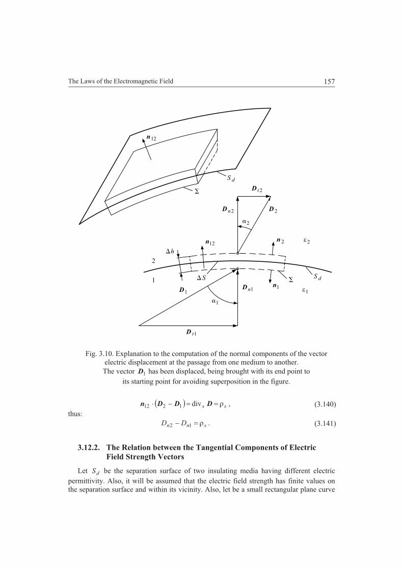
The Laws of the Electromagnetic Field 157
Fig. 3.10. Explanation to the computation of the normal components of the vectorelectric displacement at the passage from one medium to another.The vector 1D has been displaced, being brought with its end point to
its starting point for avoiding superposition in the figure.
,div1212 ss DDDn (3.140)thus:
.12 snn DD (3.141)
3.12.2. The Relation between the Tangential Components of ElectricField Strength Vectors
Let dS be the separation surface of two insulating media having different electricpermittivity. Also, it will be assumed that the electric field strength has finite values onthe separation surface and within its vicinity. Also, let be a small rectangular plane curve
12n
D t
D
2
2D n2
2
D t
DnD
S
h
2n1n 2
n11
S
1
1
1
1
2
1
2
d
S d

General Theory of the Electromagnetic Field158
having each of its long sides on one of the two sides, respectively, of the separationsurface, parallel and very near to that surface (Fig. 3.11). The length of one long side ofthe rectangular curve, parallel to the separation surface will be denoted by l and theheight, parallel with the normal to the separation surface, will be denoted by h . Thelength of l is taken small enough for to be considered as a straight-line segment. Thequantity l is assumed as an infinitesimal of the first order, and the quantity h as aninfinitesimal of a higher order.
Let the vector quantities 1E and 2E be the electric field strengths at two points verynear situated on both sides of the separation surface.
The law of electromagnetic induction in integral form, expressed by relation (3.50)will be applied for the closed curve that has a rectangular form (Fig. 3.11). Thetravelling direction along the curve of Fig. 3.11 results from the direction of the unitvectors 1t and 2t . The magnetic flux represented by the surface-integral of the right-handside of expression (3.50) of the law of electromagnetic induction, is an infinitely smallquantity of higher order, proportional to the height of the rectangle, and tends to zerotogether with that height.
Fig. 3.11. Explanation to the calculation of tangential components of electric fieldstrength vectors at the passage from one medium to another.
The vector 1E has been displaced, being brought with its end point toits starting point for avoiding superposition in the figure.
E t 2
E 2n
E 2
1
h
1
2
2
Sdt
t
Sd
n12
n 21
E t
E
nE
1
2
1
1
1
2
1

The Laws of the Electromagnetic Field 159
By neglecting the line-integrals along the height, because the height h is muchsmaller than the length l , it follows:
,021 ll tEtE (3.142)
where the vector quantity t is the unit vector of the tangent to the separation surfacealong the side of length l of the rectangle. Thus:
.021 EEt (3.143)
It results that at the passage through a separation surface between media, the tangentialcomponent of the electric field strength is conserved:
,21 tt EE (3.144 a)
.21 tt EE (3.144 b)
The last relation expresses the theorem of conservation of the tangential component of
the electric field strength.
3.12.3. The Theorem of Refraction of the Lines of Electric Field in theCase of Insulating Media
Let us consider a separation surface between two isotropic media of different electricpermittivity and we shall assume that the electric charge is distributed in space, i.e., it hasa volume distribution.
We can write:
,111 ED (3.145 a)
.222 ED (3.145 b)
At the passage through the separation surface above, the vectors electric displacementand electric field strength vary in magnitude and direction, i.e., they are refracted. FromFig. 3.10, it follows:
,tan1
11
1
11
n
t
n
t
D
E
D
D(3.145 c)
,tan2
22
2
22
n
t
n
t
D
E
D
D(3.145 d)
,tan
tan
22
2
1
11
2
1
t
n
n
t
E
D
D
E(3.145 e)
or by using the conservation theorems (3.139) and (3.144), it results that:
.tan
tan
2
1
2
1(3.146)

General Theory of the Electromagnetic Field160
Relation (3.146) represents the theorem of refraction of the lines of electric field in thecase in which the true (free) electric charge has a volume distribution. In this case, thereare not discontinuity surfaces of the true electric charge distribution. Therefore, on theseparation surface, there is not electric charge distributed with a finite surface density.
The refraction theorem expressed by relation (3.146) is similar, to some extent, to thatof Optics. However, it differs from the latter because relation (3.146) is not compatiblewith the total reflection phenomenon, since the trigonometric tangent function occursinstead of sine function in Optics. Hence, the refraction ratio (3.146) cannot havenegative values like in Optics.
3.12.4. The Relation between the Normal Components of MagneticInduction Vectors
Let dS be the separation surface of two insulating media having different magnetic
permeability. Let S be a portion of the separation surface dS . The dimensions of S
are assumed very small, hence infinitesimal entities of the first order. The portion S ofthe separation surface will be dressed by a surface having the form of a right cylinderor parallelepiped (Fig. 3.12) the height of which is an infinitesimal of a higher orderrelatively to the dimensions of the cross-section S that may be considered as a planesurface element. The bases of the parallelepiped that is a closed surface have the samedimensions like the cross-section. Let the vector quantities 1B and 2B be the magneticinductions at two points very near situated on both sides of the separation surface.
The law of magnetic flux, in integral form, expressed by relation (3.29), will beapplied for the case of the closed surface . Neglecting the flux through the lateralsurface of the parallelepiped, because its height is much smaller than the dimensions of itsbases, the following relations are obtained:
,0d SB (3.147)
,0122121 SS nBnB (3.148)
where the vector 12n is the unit vector of the normal to the separation surface dS ,
oriented from the medium 1 towards the medium 2, hence: 2121 nnn .Hence:
.0div1212 BBBn s (3.149)
It follows that at the passage through a separation surface of two media, the normalcomponent of the magnetic induction is conserved, thus:
,21 nn BB (3.150 a)
.21 nn BB (3.150 b)
The last relation expresses the theorem of conservation of the normal component of
the magnetic induction.

The Laws of the Electromagnetic Field 161
Fig. 3.12. Explanation to the computation of the normal components of the vectormagnetic induction at the passage from one medium to another.
The vector 1B has been displaced, being brought with its end point toits starting point for avoiding superposition in the figure.
3.12.5. The Relation between the Tangential Components of theMagnetic Field Strength Vectors
Let dS be the separation surface of two insulating media having different magneticpermeability. Also, it will be assumed that the electric current density has finite values onthe separation surface, hence, the electric current is not discontinuously distributed in theform of a current sheet on the separation surface. In addition, it will be assumed that theelectric displacement has finite values.
Also, let be a small rectangular plane curve having each of its long sides on one ofthe two sides, respectively, of the separation surface, parallel and very near that surface(Fig. 3.13). The length of one long side of the rectangular curve, parallel to the separation
12n
t 2
2n2
2
t
n
S
h
2n1n 2
n11
S
1
1
1
1
2
1
2
d
B
BB
B
B
B
S d

General Theory of the Electromagnetic Field162
Fig. 3.13. Explanation to the calculation of tangential components of the magneticfield strength vectors at the passage from one medium to another.
The vector 1H has been displaced, being brought with its end point toits starting point for avoiding superposition in the figure.
surface will be denoted by l , and the height, parallel with the normal to the separationsurface, will be denoted by h . The length of l is taken small enough for to beconsidered as a straight-line segment. The quantity l is assumed as an infinitesimal ofthe first order, and the quantity h as an infinitesimal of a higher order.
Let the vector quantities 1H and 2H be the magnetic field strengths at two pointsvery close one to the other situated on both sides of the separation surface.
The law of magnetic circuit in integral form, expressed by relation (3.84) will beapplied for the closed curve that has a rectangular form (Fig. 3.13). The travellingdirection along the curve results from the direction of the unit vectors 1t and 2t .
The electric flux represented by the surface-integral of the right-hand side ofexpression (3.81) of the law of magnetic circuit, is an infinitely small quantity of higherorder, proportional to the height of the rectangle, and tends to zero together with thatheight.
By neglecting the line-integrals along the height, because the height h is muchsmaller than the length l , it follows:
t 2
2n 2
1
h
1
2
2
Sdt
t
Sd
n12
n 21
t
n
1
2
H
HH
H
H
H 1
1
1
2
1

The Laws of the Electromagnetic Field 163
,021 ll tHtH (3.151)
where the vector quantity t is the unit vector of the tangent to the separation surfacealong the side of length l of the rectangle. Thus:
.021 HHt (3.152)
It results that at the passage through a separation surface between media, the tangentialcomponent of the magnetic field is conserved:
,21 tt HH (3.153 a)
.21 tt HH (3.153 b)
The last relation expresses the theorem of conservation of the tangential component of
the magnetic field strength.We shall consider the case in which an electric current is distributed on the separation
surface in the form of a current sheet (Fig. 1.12), of linear density sJ of direction
perpendicular to the plane of the figure at the points of the trace of the surface dS in the
Fig. 1.12. In this case, the current linkage is lJ s and instead of relation (3.152), weobtain:
,21 sJHHt (3.154)
thus:
.21 stt JHH (3.155)
3.12.6. The Theorem of Refraction of the Lines of Magnetic Field at thePassage through the Separation Surface of Two Media
Let us consider a separation surface between two isotropic media of different magneticpermeability and we shall assume that the electric current has a volume distribution.
We can write:
,111 HB (3.156 a)
.222 HB (3.156 b)
At the passage through the separation surface above, the vectors magnetic inductionand magnetic field strength vary in magnitude and direction, i.e., they are refracted. FromFig. 3.13, it follows:
,tan1
11
1
11
n
t
n
t
B
H
B
B(3.156 c)
,tan2
22
2
22
n
t
n
t
B
H
B
B(3.156 d)

General Theory of the Electromagnetic Field164
22
2
1
11
2
1
tan
tan
t
n
n
t
H
B
B
H(3.156 e)
or, by using the conservation theorems (3.150) and (3.153), it follows:
.tan
tan
2
1
2
1(3.157)
Relation (3.157) represents the theorem of refraction of the lines of magnetic field inthe case in which the electric current has a volume distribution. Hence, there are notdiscontinuity surfaces carrying electric current sheets.
3.12.7. The Relation between the Normal Components of ElectricDisplacement Vectors and Electric Current Densities
Let us consider the separation surface dS between two media having different electricproperties, namely different electric permittivity and conductivity. The surface is assumedcarrying no electric current sheet. The very flat parallelepiped surface of Sub-section3.12.1 (Fig. 3.10) will be considered. For the parallelepiped base of medium 1, boundedby a rectangular curve, by applying relation (3.79), we can write:
.ddd
111
11
111 S
t
DJ
tS
nn
S
SD
JlH(3.158 a)
For the parallelepiped base of medium 2, bounded by a rectangular curve, by applyingrelation (3.79), we can write:
.ddd
222
22
222 S
t
DJ
tS
nn
S
SD
JlH(3.158 b)
The curves 1 and 2 that bound the two bases tend to the same curve of very
small dimensions placed on the separation surface. The quantities lHlH dd 11 t and
lHlH dd 22 t are equal, for according to relation (3.153), 21 tt HH .The last two relations (3.158 a) and (3.158 b) yield:
.22
11
t
DJ
t
DJ n
nn
n (3.159)
and, as mentioned, the following relation
21 tt HH
subsists.

The Laws of the Electromagnetic Field 165
3.13. THE SI UNITS OF MEASURE OF ELECTRIC AND MAGNETICQUANTITIES: ELECTRIC FLUX, ELECTRICDISPLACEMENT, ELECTRIC RESISTIVITY, MAGNETICFLUX, MAGNETIC INDUCTION, MAGNETIC FIELDSTRENGTH.
3.13.1. The Units of Electric Flux and Displacement
In the SI system, the unit of measure of the flux of electric displacement, also calledelectric flux, results from relation (3.14) and it is the coulomb, symbol C, the same as forthe electric charge. From the same relation, it follows that the unit of measure of the
electric displacement (electric flux density) is 2m/C . From relation (3.18) it follows thatthe unit of measure of the electric polarization is the same as for the electricdisplacement.
3.13.2. The Unit of Electric Resistivity
In the SI system, the unit of measure of the electric resistivity results from relations(1.108) and (1.109). This unit of measure is given by the ratio of lE and J as follows:
.m1A1
V1
m/A1
m/V1
][1
][1][1
2SIJ
E
But in Electrokinetics, the ratio between one volt and one ampere is called ohm,symbol , thus:
.1A1
V1
Therefore the unit of measure of the electric resistivity is m , as follows:
.m1][1
3.13.3. The Unit of Magnetic Flux
A definition of the unit of measure of magnetic flux may be given by using the law ofelectromagnetic induction in the integral form (3.57):
.d
d
tue
In the SI system of units, the unit of measure of magnetic flux is the weber, symbolWb.
The weber is the magnetic flux that cancelling by a linear variation after a time of onesecond induces in a single turn linked by it, the electromotive force of 1 V.

General Theory of the Electromagnetic Field166
Indeed, for the linear variation with time of the magnetic flux, mentioned above, andshown in Fig. 3.14, it follows:
.11
0
d
d 00
tue
If the variation of the magnetic flux were not a linear one then the electromotive forceinduced at any instant, in the turn, would be given by the derivative of the magnetic flux.In this case, the value of the magnetic flux is more difficult to be determined than in thecase above.
3.13.4. The Unit of Magnetic Induction
In the SI system of units, the unit of measure of magnetic induction is the tesla,symbol T. A definition of the unit of measure of magnetic induction can be obtained byusing the defining relation of magnetic flux (3.32):
S
.d SB
In the case of a homogeneous magnetic field, the last relation becomes:
,SB
and if the vector quantity B is perpendicular to the considered surface, i.e., the vectorsB and S are parallel to each other, it results that:
.SB
The tesla is the magnetic induction of a homogeneous magnetic field (i.e., with a
uniform distribution), the flux of which, through a surface having the area of 2m1 , andperpendicular to the lines of the magnetic field, is of Wb1 .
Fig. 3.14. Explanation concerningthe definition of the
unit of measure of the magnetic flux.
t1 s
O
0

The Laws of the Electromagnetic Field 167
3.13.5. The Unit of Magnetic Field Strength
The unit of measure of the magnetic field strength can be obtained by using theexpression of the magnetic field strength at the centre of a circular turn carrying a directcurrent:
.2 a
iH
This expression will be established in Sub-section 3.15.2.In the SI system, the unit of measure of the magnetic field strength is the ampere per
metre, symbol m/A .Ampere per metre is the magnetic field strength at the centre of a circular turn with the
diameter of 1 m, carrying a direct current of 1 A.The unit of measure of the magnetic tension and magnetomotive force, in the SI
system of units, is the ampere, symbol A, hence the same unit of measure as for theelectric current intensity.
3.13.6. The Units of Electric and Magnetic Constants
The unit of measure of the electric constant, in the SI system of units, can be easilyobtained from relation (3.6). The unit of measure of the left-hand side of this relation is
that of the product of the quantities E , S and 0 , hence 02m)m/V( , thus
0mV . The unit of measure of the right-hand side of the same relation is that of theelectric charge, thus C . By equating the two units of measure, we obtain:
.m
1
V
C0
But in Electrostatics, the ratio V/C is defined as farad, symbol F . Therefore the unit ofthe electric constant is m/F .
The unit of measure of the magnetic constant can be easily obtained from relation(2.27 b). From these relations, it follows that in vacuo:
,0 HB
where, for the sake of simplicity, the subscript o indicating the reference frame has beenomitted.
In the last relation, the unit of measure of the left-hand side is that of B . The unit ofmeasure of the right-hand side of the same relation is that of the product of the quantitiesH , and 0 , hence 0)m/A( . But, as shown above, namely by the last relation of
Sub-section 3.13.4, this unit of B can be expressed in the form 2m/Wb . By equatingthe two units of measure, we obtain:
.m
1
A
Wb0
General Theory of the Electromagnetic Field168
But in Electrodynamics, the ratio A/Wb is defined as henry, symbol H . Therefore theunit of the electric constant is m/H . The same results could be obtained, e.g., by usingrelations (3.23), (3.24) and (3.104), (3.105), respectively.
3.13.7. Remark on the Various Systems of Units of Measure inElectromagnetism
Before the adoption of the International System of Units of Measure, and the MKSAwhich preceded it, two systems of units of measure played an important role, having ascientific value: The Electrostatic System of Units and the Electromagnetic System ofUnits [1, Arts. 625, 628].
The Electrostatic System of Units has been based on the definition of the unit ofelectric charge according to the Coulomb formula for electric charges in vacuo, with theconstant of proportionality dimensionless and equal to unity. The two charges occurringin formula are taken equal to each other. Hence the formula will contain only thequantities: force, electric charge q and a length r .
The Electromagnetic System of Units has been based on the definition of the unit ofmagnetic charge (i.e., the fictitious magnetic charge) according to the Coulomb formulafor Amperian magnetic charges with the constant of proportionality dimensionless andequal to unity. Further on, the formula of the electromagnetic force, like that exertedbetween two coils carrying electric currents, including one proportionality constant, hasalso been established using the same system of units. As shown in [1, Vol. II, Art. 628],the ratio between the unit of electric charge in the Electromagnetic System of Units, andthat of the Electrostatic System of Units, denoted by indices uem and ues, has the
dimension of a velocity, and was found to be approximately equal to 10103c cm/s. Itis just the velocity of light in empty space (vacuum) or air. The apparatus conceived andused by Maxwell for the experimental determination can be found in [4, 372].
The same result may be directly obtained by remaking the calculations concerningformulae (2.22) – (2.24), taking 40 and dimensionless. Using formula (1.113) therefollows:
,][][1;;;4
111uesuemuesuem
202
020 qcqqqcck
cc
and then we obtain the ratio above.A combination of the two systems of units, called the Gaussian System of Units, has
also been used [3], [7], [8], [11], [22], [23], [24].
3.14. THE LAWS OF ELECTROMAGNETIC FIELD IN THE CASEOF EXISTENCE OF MAGNETIC MONOPOLES
We shall further examine the modifications occurring in the laws of the theory of theelectromagnetic field, in the case of existence of magnetic monopoles. The existence ofthese monopoles has been supposed, but up to now no doubtless experiment has provedtheir existence.
The Laws of the Electromagnetic Field 169
3.14.1. Expression of the Interaction Force between TwoMagnetic Monopoles
The expression of the interaction force between two point-like magnetic charges, i.e.,monopoles, is assumed to be of the same form as the expression of the interaction forcebetween two point-like electric charges, hence an expression of the form:
12
122
12
211
021
4
1
rr
qq MM rF (3.160)
or
,4
1
12
122
12
21
021
rr
qq mm rF (3.161)
which is the Coulomb formula for magnetic charges in the case of empty space (i.e.,vacuum). The quantities introduced by relation (3.160) are called Amperian magnetic
charges, whereas the quantities introduced by relation (3.161) are called Coulombian
magnetic charges. Between these quantities we have the following relation:
.0 Mm qq (3.162)
If for the constant of the right-hand side of relations (3.160), (3.161), other value wereadopted, different units of measure would be obtained for the electromagnetic quantities.
Analogously as for the electric charges, we can consider volume distributions ofmagnetic monopoles with the volume density of the magnetic charge vM or vm ,respectively, including the suffix M or m. Also, we can consider magnetic charge withsurface distribution with the surface density sM or sm , and line distribution with the
line density lM or lm . The monopoles can be at rest or in motion.Similarly as in the case of electric charges, the following force produced by any point-
like magnetic charge 1mq placed at any point, called source point, is acting on the point-
like magnetic charge mq placed at another point, called field point or observation point:
.mmmMm qq HBF (3.163)
If we denote by 12r the vector having its origin at the source point and its end at thefield point (observation point), it follows:
,4
1
4
1
12
122
12
1
012
122
12
11
0 rr
q
rr
q mMm
rrH (3.164)
.0 mm HB (3.165)
3.14.2. Electric Field Produced by Moving Magnetic Monopoles
We shall consider the same reference frames oK and 1K , of Sub-section 2.3.2, the
latter moving at the velocity o1v with respect to the former. At any fixed point, A, in 1K ,
there is a point-like magnetic charge 1mq (the subscript 1 of 1mq has no relation with the
General Theory of the Electromagnetic Field170
subscript 1 of 1K ), and another magnetic point-like magnetic charge mq , at any point P,
moving at the velocity o2v relatively to oK . We shall consider the magnetic field
strength produced by 1mq at the point P, in empty space.We shall remake the calculations of Section 2.4, but instead of relations (2.18 a, b, c)
which are based on formula (1.112), we shall use the relations based on one of formulae(3.160) or (3.161). In order to distinguish the field state quantities due to the magneticpoint-like charge, those quantities will have the suffix m. We obtain:
(3.166 a, b);o0o mm ED ;1
oo12o mmc
HvD
.1
oo12o2oo mmmmmc
qq HvvHF (3.167)
3.14.3. The Expressions of the Laws of the Theory of the ElectromagneticField in the Case of Magnetic Monopoles
We shall make derivations similar to those for expressions: (3.5 b), (3.27), (3.47),
(3.68). The calculations include: mo0o µdiv , moocurl H , mt
oo
D , moocurl D , in oK .
The field state quantities obtained from the last relations for magnetic charges will beadded, side by side, with those previously obtained for the electric charges, as follows:
;: ooo mDDD ;: ooo mEEE ;: ooo mBBB .: ooo mHHH (3. 168)
It results that the form of relations (3.5 b) and (3.27) is not modified, while relations(3.27) and (3.68) become:
;div o0oo MvB ,curl omagoo JE ,o0o
oomag mMv
tv
BJ ,o1vmv (3.169 a-d)
where magJ may be called the magnetic current density.
3.15. APPLICATION OF THE BIOT-SAVART-LAPLACE FORMULATO THE CALCULATION OF THE MAGNETIC FIELDSTRENGTH
3.15.1. Expression of the Magnetic Field Strength Produced by aThread-Like Rectilinear Conductor Carrying aConstant Electric Current
Let us consider a rectilinear thread-like conductor of length l and constant cross-section cs carrying an electric current of intensity i shown in Fig. 3.15, in empty space.In this case, the magnetic field strength is given by relation (2.48). It follows:

The Laws of the Electromagnetic Field 171
.d
4
13r
iP
rlHH (3.170)
The vector H at the point P is perpendicular to the plane determined by the straight-line segment and the point P , and oriented so that it enters into the plane of the figure.We shall consider the modulus of the vector H . According to the symbols of Fig. 3.15,we have:
,,dsind
4
1dd
3r
rliHPH
rl(3.171)
but
cos2
sin,dsin rl (3.172)
and
.cos
;dcos
d;tan2
ar
alal (3.173)
It follows:
.sinsin4
1d
cos
coscos
4
121
2
2
2
2
1
iaa
a
iH (3.174)
For an infinitely long conductor, i.e., b , we have:
.2
;2 21 (3.175)
Fig. 3.15. Explanation to thecalculation of the magnetic field
strength produced by a rectilinearthread-like conductor carrying an
electric current.
[ ]( )
1 2
d ll
b
i
r
a
HP
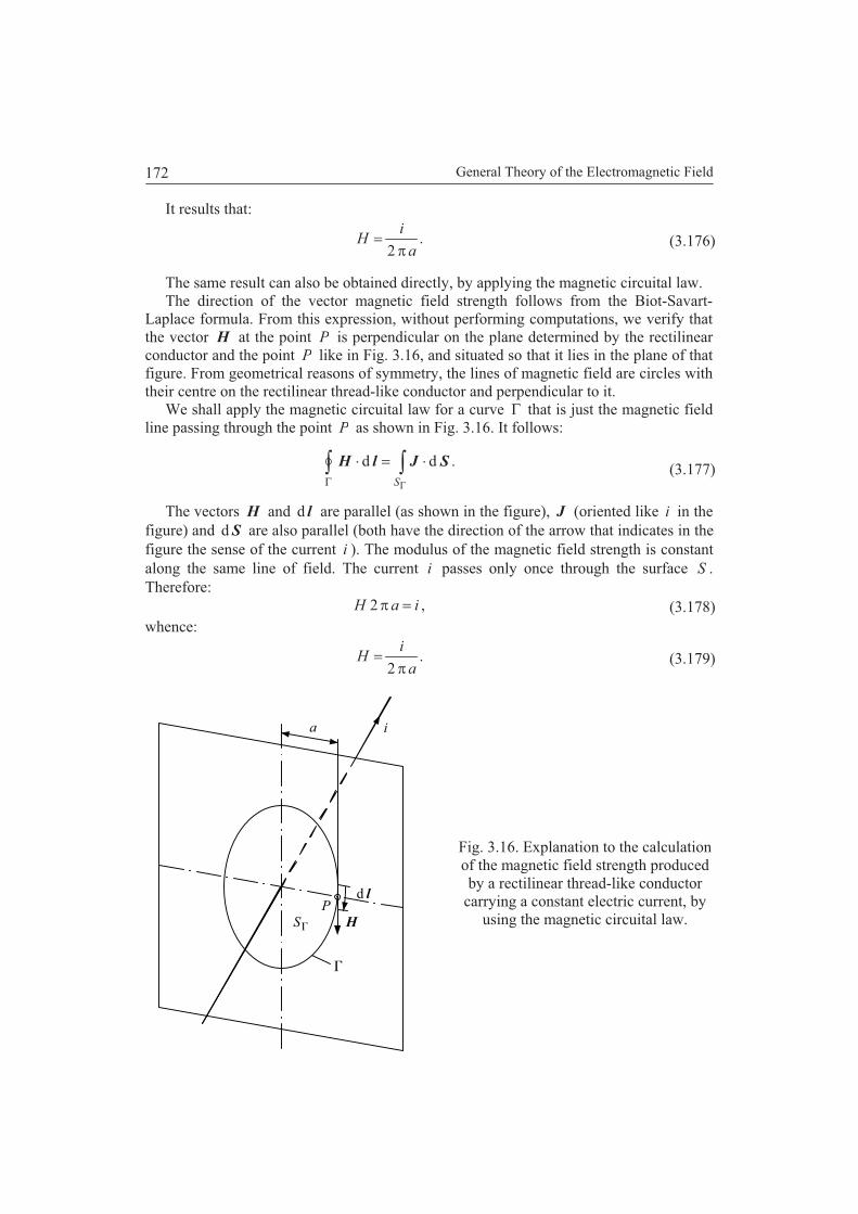
General Theory of the Electromagnetic Field172
It results that:
.2 a
iH (3.176)
The same result can also be obtained directly, by applying the magnetic circuital law.The direction of the vector magnetic field strength follows from the Biot-Savart-
Laplace formula. From this expression, without performing computations, we verify thatthe vector H at the point P is perpendicular on the plane determined by the rectilinearconductor and the point P like in Fig. 3.16, and situated so that it lies in the plane of thatfigure. From geometrical reasons of symmetry, the lines of magnetic field are circles withtheir centre on the rectilinear thread-like conductor and perpendicular to it.
We shall apply the magnetic circuital law for a curve that is just the magnetic fieldline passing through the point P as shown in Fig. 3.16. It follows:
.ddS
SJlH (3.177)
The vectors H and ld are parallel (as shown in the figure), J (oriented like i in thefigure) and Sd are also parallel (both have the direction of the arrow that indicates in thefigure the sense of the current i ). The modulus of the magnetic field strength is constantalong the same line of field. The current i passes only once through the surface S .Therefore:
,2 iaH (3.178)whence:
.2 a
iH (3.179)
Fig. 3.16. Explanation to the calculationof the magnetic field strength producedby a rectilinear thread-like conductor
carrying a constant electric current, byusing the magnetic circuital law.
a i
d l
H
PS
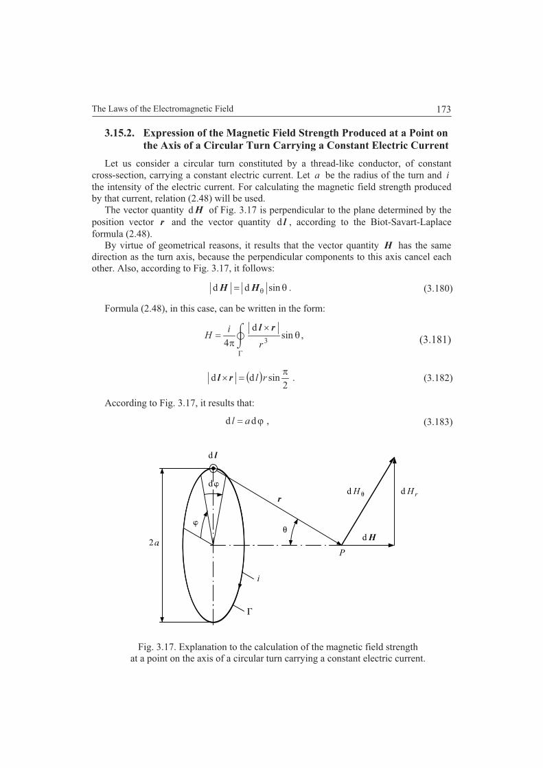
The Laws of the Electromagnetic Field 173
3.15.2. Expression of the Magnetic Field Strength Produced at a Point on the Axis of a Circular Turn Carrying a Constant Electric Current
Let us consider a circular turn constituted by a thread-like conductor, of constantcross-section, carrying a constant electric current. Let a be the radius of the turn and i
the intensity of the electric current. For calculating the magnetic field strength producedby that current, relation (2.48) will be used.
The vector quantity Hd of Fig. 3.17 is perpendicular to the plane determined by theposition vector r and the vector quantity ld , according to the Biot-Savart-Laplaceformula (2.48).
By virtue of geometrical reasons, it results that the vector quantity H has the samedirection as the turn axis, because the perpendicular components to this axis cancel eachother. Also, according to Fig. 3.17, it follows:
sindd HH . (3.180)
Formula (2.48), in this case, can be written in the form:
,sind
4 3r
iH
rl
(3.181)
2sindd rlrl . (3.182)
According to Fig. 3.17, it results that:
dd al , (3.183)
Fig. 3.17. Explanation to the calculation of the magnetic field strengthat a point on the axis of a circular turn carrying a constant electric current.
d
r
d l
d H d H r
i
Hda
P2

General Theory of the Electromagnetic Field174
.sin
ar (3.184)
After performing the substitutions and the calculation of the integral, it follows:
.sin2
sind
4
2
0
332 a
i
a
aiH (3.185)
In particular, the magnetic field strength at the centre of the turn is:
.22
sin2
3
a
i
a
iH (3.186)
The magnetic field strength produced by a circular turn carrying an electric current, ata point that is not placed on the axis of the turn, can also be calculated by the relation(2.48). In this case, elliptic integrals occur in calculation [15, p. 30].
3.16. APPLICATION OF BOTH FORMS OF THE LAW OFELECTROMAGNETIC INDUCTION FOR MEDIAAT REST AND IN MOTION
3.16.1. Calculation of the Electromotive Force Induced in a Coil inRotational Motion in a Uniform Magnetic Field
A typical example of application of various forms of the law of electromagneticinduction is the calculation of the induced electromotive forces.
We shall calculate the electromotive force induced in a coil in rotational motion in amagnetic field having the magnetic induction uniformly distributed in space. Firstly, letthe coil be constituted by a single turn.
Let
,sin 11 tBB M (3.187)
be the expression of the magnetic induction that varies with time, in a sinusoidal form,with the angular frequency 1 . The considered configuration, composed of the inductivepair of poles that produces the magnetic field and the turn in rotational motion, is shownin Fig. 3.18. The turn is in rotational motion, about one of its symmetry axes, with anangular velocity (speed) . The sizes R and l of the turn are shown in Fig. 3.18.
The electromotive force induced in the turn can be collected by a system of rings andbrushes. We shall denote by a curve taken along the conductor (wire) of which the turnis made.
The law of electromagnetic induction for media at rest will be utilized. The referenceframe will be taken fixed to the turn in rotational motion (Fig. 3.18 a). In accordance withrelation (3.118), we can assume that in the adopted moving reference frame, the magnetic

175
Fig. 3.18. Explanation to the calculation of the inducedelectromotive force in a coil in rotational motion.
xz
M
N
NM
N
S
B n
N
M
N
S
vB
B
v
v
E b
E b
v
B
B
E ld = 0b
Eb dl = 0
O
y
x
z
QP
e
n
QP
NM
2 R
l
ba
r
r
r
r
n
The Laws of the Electromagnetic Field
General Theory of the Electromagnetic Field176
induction has the same value as in the reference system considered at rest. We canarbitrarily adopt the travelling direction along the curve , and the direction of thepositive normal to the surface S will be associated according to the right-handed screw
rule. The angle determining the initial position of the turn has been denoted by 0 .The magnetic flux linked by the turn is:
,cos2 BlR (3.188)
,0t (3.189 a)
,cossin 011 ttM (3.189 b)
.2 MM BlR (3.189 c)
By using relation (3.50), it follows:
.sinsin
coscosd
dd
011
0111
tt
ttt
ue
M
Me lE(3.190)
Further on, we shall use the law of electromagnetic induction for moving media. Thereference frame will be considered fixed to the inductive poles (Fig. 3.18 b).
By applying relation (3.134) to this case, it follows:
lttBv
SttB
tue
Mr
S
M
r
S
e
dsinsin
dcoscos
ddd
011
0111
lBvSB
lE
(3.191)
or
,sinsin2
coscos
011
0111
ttlBv
ttSBue
Mr
Me(3.192)
where
.;2 RvlRS r (3.192 a, b)
If the coil of Fig. 3.18 had w turns instead of one turn, then all the inducedelectromotive forces would be w times greater.
From relation (3.134), it follows that the induced electromotive force (e.m.f.) has twocomponents: The first is a transformation component and the second is a movingcomponent (in this case a rotation component). In Fig. 3.18 b, the moving component ofthe electric field strength has been denoted by BvE rb . Also, from Fig. 3.18 b, it

The Laws of the Electromagnetic Field 177
follows that, in the front parts of the coil, the vector of the moving component of theelectric field strength bE is perpendicular to the conductor, hence:
,0dd lBvlE rb (3.192 c)
so that it does not contribute to the electromotive force.
3.16.2. Calculation of the Electromotive Force Induced by theRotation of a Magnet about Its Axis
Another typical example of application of the law of electromagnetic induction is thecalculation of the electromotive force induced between two points of one cylinder of amaterial with magnetic and conducting properties (permanent magnet), and which turnsabout its axis.
Fig. 3.19. Explanation to thecalculation of the electromotive
force induced by the rotation of onepermanent magnet in the form of a
cylinder.
VO
C
A
S
N
B
E'
v r

General Theory of the Electromagnetic Field178
The corresponding configuration is shown in Fig. 3.19. As it can be seen in Fig. 3.19,the two points C and A are situated one on the axis of the cylinder, the other on one ofits generating straight lines. The electromotive force induced between the two points canbe collected by a system of sliding contacts.
Let be the angular velocity of the rotational motion, and r the cylinder radius. Weshall consider a reference frame at rest relatively to which the cylinder is in rotationalmotion and a moving reference frame fixed to the cylinder. At any instant, we consider aclosed curve composed of a portion CO along the cylinder axis, a radius OA and a linethat closes along a conductor placed in air between the two points A and C .
At any point of the reference frame at rest, the magnetic induction does not vary. Inthis case, according to formula (3.134), it follows:
,dddd lBvlBvSB
lE r
S
ret
ue (3.193)
where rvr . If the magnetic field is assumed to be uniform, it follows:
.2
1average
2 BrvBrue re (3.194)
After the discovery of the law of electromagnetic induction (examined in Sub-section3.5.4 and Section 3.11), many discussions took place, especially in the 19th century,relatively to the possibility of interpreting the phenomenon of electromagnetic induction,in the case of a right circular cylindrical permanent magnet which turns about its axis asbeing determined by the fact that the lines of magnetic field turn together with themagnet. According to the mention of Section 2.5, that the lines of field are only anauxiliary notion and not material forms, such an interpretation is not justified.
3.17. ELECTRODYNAMIC POTENTIALS
The general equations of the electromagnetic field in local form, established above,are:
,curlt
BE (3.195 a)
,div vD (3.195 b)
,0 PED (3.195 c)
,curlt
DJH (3.195 d)
,0div B (3.195 e)
.0 jMHB (3.195 f)

The Laws of the Electromagnetic Field 179
The equations above are called the equations of the theory of electromagnetic field for
media at rest or the Maxwell equations.In many cases, for solving this system of equations, it is convenient to introduce
certain substitution functions namely: Electrodynamic scalar potential and vectorpotential, respectively. This introduction is not arbitrary, it results from the examinationof the equations above. Concerning the fifth equation, it can be remarked that thedivergence of any vector that is a curl of a field vector is always zero. Hence:
0curldivdiv AB (3.196)
and
.curl AB (3.197)
The quantity A is called vector electrodynamic potential.From the equation (3.195 a), it follows:
.0curlcurlcurlcurlttt
AEAE
BE (3.198)
In the last equation, the derivative operator with respect to t , and the operator curl thatcontains the derivatives with respect to co-ordinates can be replaced one by the other,because the two operators refer to different variables.
Concerning the last equation, it can be remarked that the operator curl of any vectorthat is a gradient of a scalar field is always zero. Hence:
.0gradcurlcurl Vt
AE (3.199 a)
It follows:
Vt
gradA
E (3.199 b)
and
.gradt
VA
E (3.200)
The quantity V of the last relation is called scalar electrodynamic potential.It is worth noting that in relation (3.199 a) we have introduced the sign minus like in
the case of potential produced by point-like charges at rest. Indeed, if the state quantitiesdo not vary with time, the relations (3.200) and (1.119) must coincide.

General Theory of the Electromagnetic Field180
3.18. THE SCALAR AND VECTOR ELECTRODYNAMICPOTENTIALS PRODUCED BY ONE POINT-LIKE ELECTRICCHARGE MOVING AT CONSTANT VELOCITY
Let oK be a reference frame assumed at rest, 1K a moving reference frame with
respect to the previous one and a material point, with a point-like electric charge 1q ,
fixed in the reference frame 1K at its origin. The velocity of the reference frame 1K and
that of the point-like electric charge 1q , fixed in the same reference frame, is assumed to
be constant .consto1o1 xviv The medium will be considered empty space (vacuum).
The electric field strength produced by the point-like charge 1q at any point
PPP zyxP 111 ,, in the reference frame 1K is:
;4
113
1
1
01 P
P
Pr
qrE (3.201)
;
,4
1
oo1oo11
2
321
21
21
11
01
tvxx
zyx
xqE
PP
PPP
PPx
(3.201 a)
;
,4
1
o1
2
321
21
21
11
01
PP
PPP
PPy
yy
zyx
yqE
(3.201 b)
.
,4
1
o1
2
321
21
21
11
01
PP
PPP
PPz
zz
zyx
zqE
(3.201 c)
The electric field strength produced by the same point-like charge 1q at the same
point PPP zyxP ooo ,, in the reference frame oK , according to relation (2.21), is:
.111o zyx EEE kjiE (3.202)
According to relation (2.26), the magnetic induction will be:
,0oxB(3.203 a)

The Laws of the Electromagnetic Field 181
,1
4
11
02
321
21
21
o111o12o
PPP
xPy
zyx
vzq
cB
(3.203 b)
.1
4
11
02
321
21
21
o111o12o
PPP
xPz
zyx
vyq
cB
(3.203 c)
According to expressions (3.203 a, b, c), it results that, in this case, the quantity oB
has components only along the oo yO and oo zO axes. According to relation (3.203 a) and(3.197), we can write that the vector potential A has a single component, namely alongthe oo xO - axis. We obtain successively:
;curlcurl oooo AiAB (3.204 a)
;;;0o
oo
o
ooo
y
AB
z
ABB zyx (3.204 b)
.11
4
1
01
o1o12o
P
xx
r
vq
cA (3.204 c)
At the initial moment, both reference frames are supposed to coincide. The point-likecharge 1q is fixed at the origin of the reference frame 1K . The observation point denoted
by P is fixed in the reference frame oK . After a time ot , the origin of the reference
frame 1K will be on the oo xO - axis at the distance oo1 tv x from the origin of the
reference frame oK . The distance between the point-like charge fixed at the origin of the
reference frame 1K and the point P marked in the same reference frame will also bemodified.
Let or be the distance between the point-like charge at the initial moment and the
point P marked in the reference frame oK . Also, let ot be equal to the time necessaryfor the field wave starting from the material point with a point-like charge that initially isat the origin, to reach the point P .
Hence, we can write:
;oo
c
rt .2
o2o
2o
2o PPP zyxr (3.205)
At the same time, we can write the relations:
oo1oo11 tvxx xPP , (3.206 a)
2
12o
2o
2oo1o
2o11 PPxPP zytvxr , (3.206 b)
General Theory of the Electromagnetic Field182
.2
2
12
1
2
12o2
2o1o
oo12
oo1
2
12o
2o2
2o12
o2
2o1o
oo12
oo1
2
12o
2o
22o
2o1ooo1
2oo1
2
12o
2o2
o1
2oo1oo11
Px
Px
PPxx
Px
PPxPxP
PPxPP
xc
v
c
rxvr
zyc
vr
c
v
c
rxvr
zytvtxvx
zytvxr
(3.206 c)
Hence:
.c
2 oo1oo1
2
12oo1oo1
o2
oo11c
rc
rrr P
rvrvrv(3.207)
Therefore, relation (3.204 c) becomes:
.11
4
1
0oo1o
o112o
cr
q
c rv
vA
(3.208)
From the expression (3.200) of the electric field strength in terms of the scalar andvector potential, we obtain:
;grado
oooo
x
xxt
VEA
(3.209 a)
;0;grado
oooo
y
yyt
VEA
(3.209 b)
.0;grado
oooo
z
zzt
VEA
(3.209 c)
The expression of oV can be obtained easily from relations (3. 209 b, c):
.4
1
4
1grad
31
o1o1
03
1
11o1
0ooo
P
P
P
Pyy
r
yq
r
yqEV (3.210 a)
It follows:
.4
1
4
1grad
31
o1o1
03
1
11o1
0ooo
P
P
P
Pzz
r
zq
r
zqEV (3.210 b)
The relations (3.210 a, b) yield:
The Laws of the Electromagnetic Field 183
.14
1
1o1
1
0o
Pr
qV
(3.211)
It follows:
.4
1
oo1o
1
0o
cr
qV
rv (3.212)
If we omit the index referring to the reference frame, we can write:
,4
1
oo1o
1
0
cr
qV
rv (3.213)
.11
4
1
0oo1o
o112
cr
q
c rv
vA
(3.214)
The last two relations represent the expressions of the scalar and vectorelectrodynamic potential, respectively, at any observation point, also called field point, inempty space (vacuum).
The field wave starting from the point-like charge is propagated with the velocity c .Let the point-like charge be at any point M at the moment of observation. The vector or
in formula above has its end at the observation point P , but its origin is not at the pointM at which the point-like charge is at the same moment but at the point at which thepoint-like charge was at a previous moment, say N . In the calculation above, thisprevious point N was chosen at the origin. The distance from the point N to the pointP is equal to the distance covered by the field wave during the time necessary to thepoint-like charge for moving from the point N to the point M . Therefore theperturbation at point N manifests at any point P not at the same moment, but later, andfor this reason, the potentials obtained above are referred to as retarded potentials.
The scalar and vector potential above, produced by a moving point-like charge arealso referred to as LIÉNARD-WIECHERT potentials.
3.19. THE SCALAR AND VECTOR ELECTRODYNAMICPOTENTIALS PRODUCED BY ONE POINT-LIKE ELECTRICCHARGE MOVING AT NON-CONSTANT VELOCITY
Let us consider a set of two material points, with the electric charges q and 1q ,
namely point-like electric charges, in the same inertial reference frame, say oK . We
suppose that the charge q has the velocity rvv o2 and the charge 1q has the velocity
1o1o1 viv v . Firstly, we shall suppose that the point-like charge that produces the

General Theory of the Electromagnetic Field184
electromagnetic field is moving at a constant velocity 1v . The equation of motion of a
material point of inertial mass m , with the electric charge q , in the electromagnetic field,giving the expression of the force acting upon the material point, established for the casein which const,1v is:
BvEvF rr qmtd
d(3.215 a)
or
,curlgradd
dAv
AvF rr
tVqm
t(3.215 b)
where V and A are the retarded electrodynamic scalar and vector potentials, also calledLiénard-Wiechert potentials produced by one moving point-like electric charge that wecould term source electric charge. As shown above by relations (3.213) and (3.214), theexpressions of these potentials at an observation (field) point, in the case in which thesource charge is moving with constant velocity, can be brought to the form:
,4
;4
1
1
110
1
1
0
c
q
c
qV
rvr
vA
rvr
(3.216 a, b)
where r is the vector having its origin (source point) at the point N , as explained afterrelation (3.214), and its end at the observation point (field point) P , at any moment t .Therefore, the quantities V and A of the left-hand side are given at any moment t by
the point-like electric charge 1q considered at the position it had at the moment c
rt .
The forces acting upon a moving point-like charge q can be obtained from the
Lagrange equation, where the generalized co-ordinates ks are used:
.0d
d
kk s
L
s
L
t(3.217)
For a system of n material points that contains k connection conditions, there areknf 3 equations. Let the Lagrange function be adopted in the form:
,AvrqVqTUTL (3.218)
with
.12
22
0c
vcmT r (3.219)
In the case above, the Lagrange function of the system of material points with electriccharge (3.218) is equal to the difference of two terms. The first one is the Lagrange

The Laws of the Electromagnetic Field 185
function T of the material point with the electric charge q when the electromagneticfield is zero. The second one is the supplementary Lagrange function U of the samematerial point with the electric charge q due to its interaction with other electric charges.
The quantity T represents, in the case of small velocities, the kinetic energy, apartfrom a constant, in other words, within to a constant. This remark can be obtained as aresult of the expansion in McLaurin series of the root square. The quantity U representsthe potential energy. These two terms do not depend on acceleration.
It can be added that, instead of the previous expression of the quantity T , also anotherexpression could be used, for example:
,112
22
0c
vcmT r (3.219 a)
however, the further results will not be affected.Now, we shall consider the case in which the velocity 1v of the point-like charge 1q
that produces the electromagnetic field is not constant with time. The Lagrange functionis assumed to not depend on acceleration. As a consequence, in the case in which theelectric charge 1q that produces the electromagnetic field has a variable velocity 1v , theexpression of the term U of relation (3.218) remains the same as in the case of a constantvelocity above. Therefore, the expressions of the quantities V and A (3.216 a, b) remainvalid in this case.
It is possible to show that for given values of the quantities V and A , the force actingupon a moving charge in electromagnetic field depends only on the derivatives of thesequantities, regardless of the form of variation of 1v .
The derivation of this force can be achieved by adopting, under a certain modification,the derivation of the work [50, Vol. I, Ch. V, Par. 60]. The modification is constituted bythe utilization of another expression of the term T and by the consideration that theinertial mass of the point-like charge q is depending on its velocity.
We shall consider only the system of co-ordinates of the reference frame oK .Therefore, no index will be used for indicating the reference frame. The Lagrangeequation, in the known form is:
,;;
;3,2,1,0d
d
321 zxyxxx
kx
L
x
L
t kk (3.220)
where the over-script dot denotes the derivative.We shall denote by mkp the component of the momentum mp corresponding to the
co-ordinate kx . The components of the momentum are given by the known relation:
.;;
;3,2,1,
321 zxyxxx
kx
Lp
kmk
(3.221)

General Theory of the Electromagnetic Field186
From relations (3.218), (3.219) and (3.221), we obtain the following partial derivative:
.
;;;
;3,2,1;1
1
321
321
2
2
1
2
2
20
zyxxxxvvv
zxyxxx
kAqxmAqc
c
v
xcm
x
Lp
rzryrxr
kk
r
k
kmk k
kjikjikjiv
(3.222)
The derivative of the momentum is:
.;;;3,2,1
,d
d
d
d
d
d
d
d
d
d
d
d
d
d
321
3
3
2
2
1
1
zxyxxxk
t
x
x
A
t
x
x
A
t
x
x
A
t
Aqxm
t
t
Aqxm
tt
pD
kkkkk
kk
mkk
(3.223)
In the case in which 1k then, xx1 , xAA1 and we obtain:
.d
d
d
d
d
d
d
d
z
Az
y
Ay
x
Ax
t
Aqxm
t
t
Aqxm
tt
pD
xxxx
xmxx
(3.224)
From the Lagrange equations (3.220) and (3.221), we obtain:
.3,2,1;d
dk
x
L
t
p
k
mk(3.225)
We shall assume that the term T does not depend on the quantities of the form kx but
only on kx . In the case in which 1k then, as above, xx1 , xAA1 and we get:
.d
d
x
Az
x
Ay
x
Axq
x
Vq
x
L
t
pD zyxmx
x (3.226)
By equating the right-hand sides of relations (3.224) and (3.226), we obtain:
.
d
d
x
Az
x
Ay
x
Axq
x
Vq
z
Az
y
Ay
x
Ax
t
Aqxm
t
zyx
xxxx
(3.227)

The Laws of the Electromagnetic Field 187
The force is:
.d
d
x
A
z
Az
y
A
x
Ayq
t
A
x
Vqxm
tzxxyx (3.228)
By adding up, side by side, the relations for the three axes, it follows:
.curlgradd
dAv
Av rr q
tVqm
t(3.229)
Therefore, in accordance with relations (3.200) and (3.197), we have the expressions:
;curl;grad ABA
Et
V (3.230 a, b)
where V and A are the expressions of retarded electrodynamic potentials, given byrelations (3.213) and (3.214) which have been considered to be valid for any variationwith time of the velocity 1v . The expressions of the quantities E and B given by thelast two expressions (3.230 a, b) and (3.228) yield relation (2.30) which represents theexpression of the force acting upon a point-like electric charge in electromagnetic field.Therefore, there are reasons to assume that the laws established for a constant velocity 1v
may also be considered valid for a varying velocity.

General Theory of the Electromagnetic Field188

4. THE ENERGY OF THE ELECTROMAGNETIC FIELD
We recall that, the energy of a physical system in any state, with respect to onereference state, arbitrarily chosen, is the sum of the equivalent work of all actions exertedupon the other systems, when the examined physical system passes, in any manner, fromthe state under consideration to the reference state.
Also we are recalling that the equivalent work of any action is the work necessary toproduce the respective action, or the work that would be obtained by suppressing therespective action.
The energy satisfies a conservation law as follows. The same value of the energy of aphysical system in the actual state (present state), with respect to the reference state, willbe obtained, regardless of the sequence of transformations undergone by the physicalsystem when passing from the reference state to the actual state (final state). Therefore,the energy of a physical system can be expressed only in terms of the state quantities thatdetermine the actual state (final state) and the reference state.
4.1. THE EXPRESSION OF THE ENERGY OF THEELECTROMAGNETIC FIELD. POYNTING VECTOR.
We shall establish the expressions of the energy of the electromagnetic field in termsof macroscopic quantities.
From a macroscopic point of view, let us consider the electric charge having a volumedistribution with the volume density v . The set of particles of the volume element vd is
charged with the quantity of electricity vq v dd . We consider that the centre of massof the set of particles electrically charged of the volume element is moving at the velocity
rv in the electromagnetic field of a domain of Fig. 4.1. The macroscopic statequantities of the field will be denoted by E and B . The force acting upon the volumeelement containing the electric charge qd is given by relation (2.30):
,dd BvEF rlq (4.1)
where
,il EEE (4.1 a)
,dd vq v (4.1 b)
and
.dd vvrl BvEF (4.2)
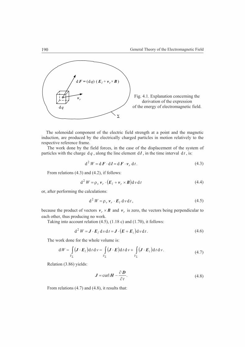
General Theory of the Electromagnetic Field190
Fig. 4.1. Explanation concerning thederivation of the expression
of the energy of electromagnetic field.
The solenoidal component of the electric field strength at a point and the magneticinduction, are produced by the electrically charged particles in motion relatively to therespective reference frame.
The work done by the field forces, in the case of the displacement of the system ofparticles with the charge qd , along the line element ld , in the time interval td , is:
.ddddd2 tW rvFlF (4.3)
From relations (4.3) and (4.2), if follows:
tvW rlrv ddd2BvEv (4.4)
or, after performing the calculations:
,ddd2 tvW lrv Ev (4.5)
because the product of vectors Bvr and rv is zero, the vectors being perpendicular toeach other, thus producing no work.
Taking into account relation (4.5), (1.18 c) and (1.70), it follows:
.ddddd2 tvtvW il EEJEJ (4.6)
The work done for the whole volume is:
.ddddddd vtvtvtW
V
i
VV
l EJEJEJ (4.7)
Relation (3.86) yields:
.curlt
DHJ (4.8)
From relations (4.7) and (4.8), it results that:
d d qF = ( ) ( E v B+ + )rl
v r
d q
The Energy of the Electromagnetic Field 191
.ddcurld vtt
W
V
iEJD
EHE(4.9)
Taking into account the vector relation:
,curldivcurl EHHEHE
it follows:
.ddcurldddivd vtt
vtW
V
i
V
EJD
EEHHE(4.10)
Taking into account relation (3.53):
,curlt
BE
we have:
,dddddddivdV
i
VV
vtvttt
vtW EJB
HD
EHE(4.11)
or, performing the transformation of a volume integral into a surface integral (Gauss-Ostrogradski theorem), the preceding relation yields:
.dddd
d
V
i
V
vvttt
WEJ
BH
DESHE
(4.12)
In the case of an isotropic and linear medium, we have the relations (3.24), (3.105):
,; HBED
and relation (4.12) gets the simpler form:
.dd2
1
2
1d
d
d
V
i
V
vvtt
WEJBHDESHE (4.13)
In relations (4.11), (4.12) and (4.13), the following symbols will be used:
,HE (4.14)
vW
V
e d2
1DE (4.15 a)
or

General Theory of the Electromagnetic Field192
,dd
0
D
D
DE vW
V
e (4.15 b)
vW
V
m d2
1BH (4.16 a)
or
,dd
0
B
B
BH vW
V
m (4.16 b)
,meem WWW (4.17)
.d SrP (4.18)
Using the symbols above, relation (4.13) becomes:
V
ime vt
W
t
W
t
W.dd
d
dEJS (4.19)
By equating the expressions of t
W
d
d from relations (4.7) and (4.19), it follows:
t
W
t
Wv me
VV
SEJ dd (4.20)
or
.d
dd r
me
V
i Pt
W
t
W
t
WvEJ (4.21)
In the relations above, only macroscopic quantities occur.In the case of bodies moving with any velocity sv relative to the reference frame, the
quantities J and E of relation (4.20) can be replaced by using relation (3.124) and(3.118). Hence, it is possible to highlight terms of the form vs dvBJ that representthe work done in the unit of time, by the force produced by the magnetic field and whichacts upon the volume element vd . This work is different from zero if vectors J and sv
are not in the same direction.In the case in which microscopic quantities are considered, relations of the same type
will be obtained, with the mention that the macroscopic quantities have to be replaced bythe microscopic ones. If no special mention is made, it will be assumed that themacroscopic energy is considered.
If the domain contains the whole space, and the electric charges, at rest or in motion,that produce the electromagnetic field are at finite distance, then the state quantities on
The Energy of the Electromagnetic Field 193
the surface at infinity are zero and the term given by relation (4.18), in relation (4.19),vanishes. The simple case in which the strength of the impressed electric field is zero,hence 0iE , will be considered. In this case, relation (4.19) represents the law ofenergy conservation for the physical system of domain , which can be expressed asfollows. The work of the forces produced by the electromagnetic field, done in the unit oftime, is equal to the decrease of the energy of the electromagnetic field, given by relation(4.19), in the unit of time.
In the case in which the strength of the impressed electric field is different from zero,the relationship of the sentence above has to be correspondingly completed.
The energy of the electromagnetic field emW contains a term eW that contains only
state quantities of the electric field, given by relation (4.15), and a term mW that containsonly state quantities of the magnetic field, given by relation (4.16). For this reason, thefirst term eW of relation (4.17) is called energy of the electric field, and the second term
mW of relation (4.17) is called energy of the magnetic field.It is interesting to be added that if the energy of electromagnetic field of any domain is
expressed in two inertial reference frames, the obtained values are not equal each other[11, p. 412].
As previously mentioned, the expressions of the macroscopic energy of theelectromagnetic field and of the microscopic energy have the same form. As shown inSub-section 1.6.6, by calculating the average values of the microscopic state quantities ofthe electromagnetic field, the macroscopic state quantities of electromagnetic field will beobtained. In the expression of the microscopic energy of electromagnetic field, theproduct of two microscopic quantities occurs. Hence, it is no more possible to state that,in general, by calculating the average value of this product, the above expression of theenergy in terms of the macroscopic state quantities will result. For this reason, in general,the macroscopic energy will not be obtained by calculating the average value of themicroscopic energy.
The relation (4.19), for 0iE , expresses, generally, the law of energy conservationof the physical system of the domain , which can be enounced as follows. The decreaseof the energy of the electromagnetic field in the unit of time is equal to the work done bythe forces produced by the electromagnetic field in the unit of time, plus a supplementaryterm that depends only on the state quantities on the domain boundary surface, and whichrepresents the radiated energy through the surface in the unit of time.
The vector HE is termed flux density vector of the electromagnetic energy orPoynting vector.
According to relations (4.15 a), (4.16 a) and (4.17), the volume density of the
electromagnetic energy (for linear media) is:
.2
1BHDEemw (4.22)
The quantities
,dV
j vP EJ (4.23)

General Theory of the Electromagnetic Field194
and
EJvt
Wp j dd
d2
(4.24)
represent the power and the volume density of the same power transferred to the bodies ofthe domain, due to the action of the forces of electromagnetic nature of the field.
The relation (4.21) represents the theorem of electromagnetic energy, for linear media.This theorem can be expressed as follows.
The decrease speed of the electromagnetic field energy of a domain bounded by aclosed surface, plus the power delivered by the sources of the impressed electric field isequal to the sum of the power transferred to the bodies contained inside the domain (dueto the work of the forces of electromagnetic nature) and the flux of electromagneticpower through the domain boundary surface.
It is no possible to give an exact and general expression of the macroscopicelectromagnetic energy in the case of substances with irreversible electric or magneticpolarization because, in this case, the polarization process is accompanied by local non-electromagnetic transformations.
The case of media containing substances with reversible polarization will beconsidered. Also, it will be assumed that 0iE . In this case, relation (4.11) yields:
.dddddddVV
vvtW BHDESHE (4.25)
The last two terms of the right-hand side of relation (4.25) represent the increase of theinternal energy if the transformations take place at constant entropy, but it is moreconvenient to consider transformations at constant temperature; then the respective termsrepresent the increase of the free energy (12, tome 3, p. 222).
From relations (4.25) and (4.7), the following two relations can be obtained:
,dddd
dd
d
d
00
vtt
W
V
SS
BHDES (4.26)
,dddd
ddd
00
vt
v
V
SSV
BHDESEJ (4.27)
where the corresponding integrals are calculated starting from the values that characterizethe reference state denoted by 0S .
The reference state for the electromagnetic energy is generally characterized, by thevalues zero of the state quantities of the electromagnetic field.
In order to bring a physical system from this reference state to another state (presentstate or actual state, i.e., final state) that differs from the reference state only by thequantities of the local state of the electromagnetic field, it is necessary to do, from theexterior of the system, actions, the equivalent work of which must be equal to theelectromagnetic energy in present (final) state.
The Energy of the Electromagnetic Field 195
In accordance with the concept of field, the electromagnetic energy is distributedthroughout the space with a certain volume density that depends on the values of the localstate quantities of the electromagnetic field.
The reference state for calculating the macroscopic electromagnetic energy is chosenaccording to the properties of the medium.
In media in which the couple of vector quantities E , D and H , B , respectively,cancel simultaneously (i.e., in media with temporary reversible polarization or in vacuo),the reference state is characterized by the following values of the state quantities 0E ,
0D , 0H , 0B .In media with permanent polarization, the reference state is characterized by the
following values of the field state quantities: 0E , 0H , 0D , 0B . In the right-hand side of expression (4.27), the first term represents the expression of the radiatedpower; the first term within square brackets represents the energy of the electric field, andthe second term, within the same brackets, the energy of the magnetic field.
4.2. THE THEOREM OF IRREVERSIBLE TRANSFORMATION OFELECTROMAGNETIC ENERGY IN THE CASE OFHYSTERESIS PHENOMENON
The case of bodies submitted to an electric or magnetic irreversible polarization, likein Fig. 3.2 and Fig. 3.9 will be considered. In this case, a part of the energy is transformedirreversibly in internal energy of the body. The volume density of the energy qw that is
transformed into internal energy of a body submitted to an electric or magneticpolarization cycle, also termed loop, is proportional to the area of the loop, i.e., the areaof the hysteresis loop, as follows:
,ddMCycleECycle
BHDEqmqeq www (4.28)
where the symbols Cycle E and Cycle M mean the cycle (also called loop) of electric andmagnetic polarization, respectively. In relation (4.28), each integral is proportional to thearea of the corresponding hysteresis loop.
The relation (4.28) expresses the theorem of irreversible transformation of
electromagnetic energy due to polarization loops. This theorem is also called Warburg
theorem [22, p. 464].
4.3. THE THEOREM OF IRREVERSIBLE TRANSFORMATIONOF ELECTROMAGNETIC ENERGY INTO HEAT
From the microscopic point of view, using a simplified model, when an electriccurrent flows in a metallic body, for instance along a conducting wire, the forces actingupon the moving charge carriers of the current, i.e., the electrons, do an internal work.The electrons cede energy by collision to the crystalline lattice of the body, and therefore

General Theory of the Electromagnetic Field196
the thermal agitation of ions and atoms of the crystalline lattice will increase and athermal effect occurs.
The expression of the electromagnetic power converted into heat can be obtainedusing formulae (4.6), (1.108), (1.109). We shall consider the case in which no otherphenomenon exists, the electric current flowing in a conducting metallic body excepted.The formulae (1.108) and (1.109) can be written in the form:
.JEl (4.29)
Formulae (4.6) and (4.29) yield:
.ddddd 22 tvtvW l JEJ (4.30)
We introduce the symbol JP in relation (4.30) for the energy converted in the body,per unit of time, i.e., the power, into heat and we get:
.ddd
ddd 2
2
vvt
WPvp lJJ JEJ (4.30 a)
It results that the electromagnetic energy converted into heat per unit of time, i.e., thepower converted when an electric conductive body of volume V carries electriccurrents, is given by the expression:
,d2
V
J vP J (4.31)
and the volume density of this power is given by the relation:
.2JJp (4.32)
The two last formulae express the integral form and the local form of the law of the
electro-heating effect or electro-calorific effect. This law is referred to as the Joule lawand is also known as the Joule-Lenz law.
The examined transformation is an irreversible one.The law above can be derived in the framework of the microscopic theory by
calculating directly the collision forces and the corresponding work [23, Vol. II, p. 46].
4.4. THE THEOREM OF ELECTROMAGNETIC MOMENTUM
Let us consider a system of n bodies or particles each of mass km and velocity
).,..,2,1(, nkkv , electrically charged and which are moving in empty space, in anyelectromagnetic field. Let us denote by any closed surface that contains the system ofbodies or particles. We shall calculate the resultant force acting upon the system ofparticles. In order to simplify the relations we suppose that the impressed field does notexist, i.e., 0iE . If impressed fields existed, the final relation could be correspondinglycompleted.

The Energy of the Electromagnetic Field 197
If the considered system contains conducting bodies, the macroscopic quantities haveto be introduced. However, the form of relations will be the same.
We shall denote by rv the velocity of the substance from the volume element, in
which the volume density of the electric charge is v .
By relation (4.2), for 0iE , we obtain:
,d v
V
rvv BvEF (4.33)
but according to relation (1.70), rv vJ . Hence, relation (4.33) can be written:
.d v
V
v BJEF (4.34)
By replacing the force by the derivative of momentum, it follows:
,dd
d
1
vmt
V
v
n
k
kk BJEv (4.35)
or
.
,dd
d
1
BJEf
fv
v
V
n
k
kk vmt (4.36)
By replacing the vector quantity J with its expression from relation (3.86), it follows:
BD
HEft
v curl
or
.curl BD
HBEft
v (4.37)
The case of empty space, i.e., vacuum, will be considered; according to relations(3.24), (3.105), we have ED 0 and HB 0 .
Relation (4.37) becomes:
.curl 00000tt
v
HEHEHHEf (4.38)
By using relation (3.53), it results that:
BEEEBHEft
v 00 curlcurl (4.39)

General Theory of the Electromagnetic Field198
or, by using relation (3.16), we obtain:
.curl1
curldiv 00
00 BEBBEEEEft
(4.40)
Taking into account relation (3.31) applied to the present case in which HB 0 , wecan write:
.curldivcurldiv 0000 HEHHHHEEEEft
(4.41)
By replacing expression (4.41) into relation (4.36), we obtain:
,dddd
d321
1 VVV
n
k
kk vvvmt
fffv (4.42)
.
,curldiv
,curldiv
003
02
01
HEf
HHHHf
EEEEf
t
(4.43 a, b, c)
We shall examine the first integral of the right-hand side of relation (4.42):
.d11 v
V
fF (4.44)
This integral can be transformed into a surface integral. For this purpose, we multiplyboth sides of relation (4.44) by any constant vector C , and we obtain:
.d11 v
V
fCFC (4.45)
The quantity under the last integral can be written:
.curldiv01 EECEECfC (4.46)
We shall take into consideration the vector relation (A.1.70) for this case:
.graddivdiv aCaaaCaaC
But, taking into account that the vector C is constant, relation (A.1.74) yields:
.curlgrad aCaCaC
Hence:
.curldivdiv aCaaCaaaCaaC

The Energy of the Electromagnetic Field 199
But
.grad2
1 2aCaCa
Therefore:
aaCaCaaCaaC curlgrad2
1divdiv 2
or
.2
1graddivcurldiv 2
aCaaCaaCaaC
But, according to relation (A.1.70), taking into account that const,C we have:
.2
1div
2
1grad 22
aCaC
It follows:
.2
1divdivcurldiv 2
aCaaCaCaaC (4.47)
By using the vector relation (4.47), relation (4.45) becomes:
vv
VV
d2
1divd 2
01 ECEECfC
or
.d2
1d
2
1d 2
02
01 Sv
V
nCEnEECSECEECfC
It results that:
.d2
1d 2
001 Sv
V
nEEnECfC (4.48)
It follows:
.d2
1d 2
001 Sv
V
nEEnEf (4.49)
The second integral of the right-hand side of relation (4.42) can be analogouslymodified:

General Theory of the Electromagnetic Field200
.d2
1d 2
002 Sv
V
nHHnHf (4.50)
The third integral of the right-hand side of relation (4.42) cannot be transformed into asurface-integral.
By replacing relations (4.49) and (4.50) into relation (4.42), we obtain:
.dd
d
d2
1
2
1
d
d
00
20
2000
1
V
n
k
kk
vt
Smt
HE
nHEHnHEnEv
(4.51)
Also, it follows:
,d2
1
2
1
d
d 20
2000
1
Smt
n
k
kk nHEHnHEnEGv
(4.52)
and
,dd
d
1
Smt
n
k
kk tGv (4.53)
where
VV
vv ,dd 00 HEgG (4.54 a)
,00 HEg (4.54 b)
.2
1
2
1 20
2000 nHEHnHEnEt (4.54 c)
The quantity G is termed electromagnetic momentum or electromagnetic quantity of
motion, and the quantity g is called volume density of the electromagnetic momentum.The quantity t is called density of the surface tension (also called the Maxwell stress
tensor) with two components, an electric one (which contains only electric statequantities) and another magnetic one (which contains only magnetic state quantities).
The quantity given by relation (4.54 a) can be physically interpreted taking intoaccount the following considerations. Let us consider the system of bodies or particlestogether with the corresponding electromagnetic field as representing an isolated physicalsystem. In this case, the surface-integral of the right-hand side of relation (4.53) vanishes.

The Energy of the Electromagnetic Field 201
It follows that for the isolated system constituted by bodies or particles, the conservedquantity is not the mechanical momentum, like in Classical Mechanics, but the sum of themechanical momentum and the quantity G , which can be interpreted as a momentumassociated with the electromagnetic field, called total momentum.
Relation (4.52) or (4.53) represents the theorem of electromagnetic momentum. Itfollows that, for a system of bodies or particles together with the field, the sum of thetensions on the surface which contains this system is equal to the velocity of the
decrease of the total momentum (mechanical plus electromagnetic), i.e., n
k
kkm1
Gv ,
located within the volume V .A detailed and general analysis of the theorem of energy and electromagnetic
momentum (also called quantity of motion) for electrically and magnetically polarizedmedia can be found in works [59], [60].

General Theory of the Electromagnetic Field202

APPENDICES


APPENDIX 1
VECTOR CALCULUS
In this Appendix, we shall recall some definitions and certain more used relations. Atthe same time, certain more important parts of the proofs will be given.
A.1.1. VECTOR ALGEBRA
A quantity that can be characterized by a single number, in any system of units, iscalled scalar quantity.
The most typical scalar is an abstract number. Other examples: temperature, mass,density, energy.
A vector is a quantity characterized by a number, termed its magnitude, expressed incertain units of measure, and a certain direction in space that includes a certain orientation(sense). There are also other definitions of vector quantities [54].
The simplest example of a vector is constituted by a straight-line segment denoted AB
having its magnitude equal to its length (i.e., the length of AB ) and a direction orientedfrom the point A towards the point B as shown in Fig. A.1.1.
Other examples of vector quantities: the force, the velocity (speed), the acceleration. A
vector may be denoted by one of the following symbols: AB , a , a or a . We shall usethe second one. The magnitude of a vector is called the modulus of the vector and isdenoted:
.aa (A.1.1)
According to their application point, the vectors can be grouped into three categories:free vectors, sliding vectors and bound vectors.
The free vectors have a given magnitude and direction, but their application point isarbitrary, for instance: the moment of a couple of forces.
The sliding vectors have a given magnitude and direction, but their application pointcan be arbitrarily chosen along a given straight line called support straight line thedirection of which coincides with that of the vector, for instance a force.
Fig. A.1.1. Representation of a vector.
A
B

General Theory of the Electromagnetic Field206
The bound vectors have a given magnitude, direction, and application point. Forinstance, a vector field, (field of vectors) is a field of bound vectors.
For the analytical definition of a vector in space, it is necessary to know the followingdata. For a free vector: 3 quantities, namely its projections along the axes of co-ordinates.For the sliding vectors: 5 quantities, the projections along the axes of co-ordinates and theparameters of the direction of the support straight line. For the bound vectors: 6quantities, the projections along the axes of co-ordinates and the co-ordinates of theapplication point.
The vector having its magnitude equal to unity is called unit vector. The unit vector ofany vector has its magnitude equal to unity, the same direction as the considered vector,
and has no physical dimension. The unit vector of a vector a can be expressed as a
a.
Two vectors a and b are equal to each other if their magnitudes are equal and theirunit vectors have the same direction.
A vector can be expressed in a three-orthogonal rectilinear system of co-ordinates(Cartesian system of co-ordinates) in the form:
,zyx aaa kjia (A.1.2)
where the quantities i , j , k are the unit vectors of the axes of co-ordinates Ox , Oy ,
Oz , and the quantities xa , ya , za are the components of the vector a along the axes of
co-ordinates Ox , Oy , Oz .a. The scalar product ba of vectors a and b :
,zyx aaa kjia (A.1.3)
zyx bbb kjib (A.1.4)
is:
.,cos zzyyxx babababa baabba (A.1.5)
b. The vector product ba of vectors a and b is the vector perpendicular to vectorsa and b and having its modulus equal to the area of the parallelogram constructed onthese vectors, hence:
;,sin baba ba (A.1.6)
;xyyxzxxzyzzy
zyx
zyx babababababa
bbb
aaa kji
kji
ba (A.1.7)
.abba (A.1.8)
The orientation (sense) of the vector ba is determined from the condition that thevectors a , b and ba to constitute a right-handed system, like in Fig. A.1.2.
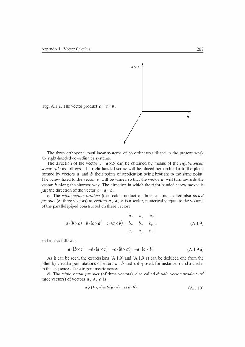
Appendix 1. Vector Calculus. 207
Fig. A.1.2. The vector product bac .
The three-orthogonal rectilinear systems of co-ordinates utilized in the present workare right-handed co-ordinates systems.
The direction of the vector bac can be obtained by means of the right-handed
screw rule as follows: The right-handed screw will be placed perpendicular to the planeformed by vectors a and b their points of application being brought to the same point.The screw fixed to the vector a will be turned so that the vector a will turn towards thevector b along the shortest way. The direction in which the right-handed screw moves isjust the direction of the vector bac .
c. The triple scalar product (the scalar product of three vectors), called also mixed
product (of three vectors) of vectors a , b , c is a scalar, numerically equal to the volumeof the parallelepiped constructed on these vectors:
,
zyx
zyx
zyx
ccc
bbb
aaa
bacacbcba (A.1.9)
and it also follows:
.bcaabccabcba (A.1.9 a)
As it can be seen, the expressions (A.1.9) and (A.1.9 a) can be deduced one from theother by circular permutations of letters a , b and c disposed, for instance round a circle,in the sequence of the trigonometric sense.
d. The triple vector product (of three vectors), also called double vector product (ofthree vectors) of vectors a , b , c is:
.baccabcba (A.1.10)
a
b
a +b

General Theory of the Electromagnetic Field208
e. Calculation of the derivative of a vector with respect to a parameter. If the vectorsare functions of a scalar variable, by applying the usual rules of differentiation, it follows:
,d
d
d
d
d
d
ttt
baba (A.1.11 a)
,d
d
d
d
d
da
aa
ttt(A.1.11 b)
,d
d
d
d
d
d
ttt
ba
ab
ba(A.1.11 c)
.d
d
d
d
d
d
ttt
bab
aba (A.1.11 d)
A.1.2. VECTOR ANALYSIS
A.1.2.1. Scalar and Vector Fields
By a scalar or a vector field, is meant a domain of space where a scalar or a vectorquantity is associated with every point. Each point of space is determined by the positionvector. Therefore, the characterization of a scalar or vector field is equivalent with theadoption of a scalar function r or a vector function ra that are depending on theposition vector r . A scalar field and a vector field can also be referred to as a field ofscalars and a field of vectors, respectively. For scalar and vector, the plural form has beenused since, at every point of the considered domain, there is a certain scalar and vector,respectively. The functions r and ra can depend apart from the position vector r ,
also on other scalar arguments, for example on time. The functions r and ra areconsidered continuous and differentiable with respect to all arguments. We shall considerthe scalar function zyx ,,r . Examples of such fields: the temperature field of abody non-uniformly heated, the density field of a non-homogeneous body, the field of anelectrostatic potential, the field of a magnetic potential.
A domain is called connected domain, if any two points belonging to the domain canbe joined by a continuous curve that belongs in totality to this domain.
A domain is called simply connected domain, if any closed curve that belongs intotality to this domain can be reduced to a single point by continuous deformationswithout overstepping the domain. The domains that have not this property are calledmultiply connected domains (doubly connected, triply connected, etc.).
Examples of simply connected domains: the interior of a sphere, the interior of acylinder of finite length, the exterior of a cylinder of finite length.
Examples of multiply connected domains: the exterior of a cylinder of infinite length,the interior of a torus.

Appendix 1. Vector Calculus. 209
A.1.2.2. The Derivative of a Scalar Function in Regard to a GivenDirection
We shall consider a spectrum composed by the lines of field, represented bycontinuous lines, and traces of potential surfaces, represented by dashed lines, like inFig. 1.3, where the direction (sense) in which we have chosen to travel the lines of fieldhas been represented by an arrow.
Let us consider that the scalar function has the value 0 at any point 0M and after
one displacement sMM 0s along the direction of a vector s , the point goes from the
point 0M to the point sM , where the scalar has the value s , like in Fig. A.1.4.The increment of the quantity , after this displacement, is:
.0s
The limit of the ratio of this increment to the magnitude of the displacement s is
denoted bys
and is called the derivative of the scalar at the point 0M in regard to
the direction s :
.lim 0
0 ss
s
s(A.1.12)
The value of this derivative depends on the direction of the vector s .For this reason, the derivative of a scalar function along a given direction must not be
confused with a usual partial derivative with respect to any variable s .
Fig. A.1.3. Plane section perpendicularto a configuration with plane parallelsymmetry, spectrum: lines of field –
continuous lines; traces of equipotentialsurfaces – dashed lines. 0
0
0
0 2
M
M 1
0

General Theory of the Electromagnetic Field210
Fig. A.1.4. Explanation to thecalculation of the derivative of ascalar function with respect to
a certain direction.
In order to study the dependence of the value of the derivatives
on the direction of
differentiation s , we shall consider the points of the field at which the function has the
same value for instance 0 . In the general case, the set of these points forms a surfacethat is termed level surface or equipotential surface. This surface has the equation:
.,, 0zyx (A.1.13)
Fig. A.1.3 shows one section made by a plane through a set of equipotential surfacescorresponding to certain values of the function equal to 0 , 0 , 20 .
A.1.2.3. The Gradient
We shall denote by n the unit vector of the normal to the level surface 0 , at a
point 0M of Fig. A.1.4, oriented in the direction assumed as corresponding to the
ascending values of the function . We shall show that in the case, in which the value of
the derivatives
with respect to the direction of this normal is known, it is possible to
calculate the value of the derivative of the scalar function with respect to any directions . We consider the equipotential surface having the ordinal number 1 that passes throughthe point sM situated on the direction s , like in Fig. A.1.4.
Let us consider two neighbouring points zyxM ,,0 and zzyyxxM ,,0 ,
both on the equipotential surface const,, 0zyx . Then, we have:
,0,,,, zyxzzyyxx (A.1.14)
both functions of the left-hand side having the same value, since they are taken for twopoints belonging to the same equipotential surface.
Therefore, the expression of the total (exact) differential of the function 0 ,
calculated at any point zyxM ,,0 , as the three quantities x , y , z tend to zero, is:
0M
M 1
0
sM s
n s
1
0

Appendix 1. Vector Calculus. 211
.0ddd zz
yy
xx
(A.1.15)
The last expression can be considered as the scalar product of two vectors:
,zyx
kjia (A.1.16 a)
.ddd zyx kjib (A.1.16 b)
Since the scalar product of the two vectors is zero, it follows that the two vectors areperpendicular to each other. The second one is a very small vector contained by thesurface const.,, 0zyx Therefore, the first vector is perpendicular to the second
one. The second vector, with the origin at the point zyxM ,,0 , can have any direction,
provided it remains contained by the surface const,, 0zyx . According torelation (A.1.15), it follows that the first vector is perpendicular on the surface
const,, 0zyx at the point zyxM ,,0 ; hence it has the direction of the positivenormal to the surface at the same point. The positive direction is considered that alongwhich the value of the function zyx ,, is assumed to increase. This vector, denotedabove by a , is called the gradient of the function . The usual symbol is:
.gradzyx
kji (A.1.17)
Let us calculate the derivative of the function zyx ,, at the same point zyxM ,,0
like above along any direction s . The expression of this derivative is:
,lim 0
0 s
MM
s
s
s(A.1.18 a)
where:,sss
(A.1.18 b)
,,, 0zyxM r(A.1.18 c)
.,, sss zzyyxxM srr (A.1.18 d)
Therefore:
,,,,,
lim0 s
zyxszsysx
s
zyx
s(A.1.18 e)
where the vector s is the unit vector of s .By expanding in a series and retaining only the small quantities of the first order, we
get:
General Theory of the Electromagnetic Field212
.d
d
d
d
d
d
s
s
zs
s
ys
s
xs
zyx (A.1.19 a)
Therefore:
.sksjsizyxs
(A.1.19 b)
Hence:
.grad skjikji zyx ssszyxs
(A.1.19 c)
From the last relation, it follows that the greatest value of the left hand-side, at a point,of this relation is obtained in the case in which the vector s has the direction of thegradient vector, hence the one of the normal at the same point of the surface, thus ns .Therefore:
;grad nn
.grad nn
(A.1.20 a, b)
Therefore:
.snns
(A.1.21)
It follows that the greatest value of the derivative of a function of point is obtained ifthe derivative of that function is calculated along the direction of the positive normal tothe equipotential surface that passes through the considered point. Otherwise, the valuewould be smaller, because the scalar product sn is a cosine.
The vector nn
oriented along the normal to the equipotential surface in the
direction of the increasing values of the function , as said above, is called the gradient
of the scalar function and is expressed by the relation above.Therefore, the derivative of the function with respect to the direction s is equal to
the projection of the vector grad along the direction s .In a three-orthogonal rectilinear system of co-ordinates, according to relations
(A.1.20) and (A.1.21), it follows:
,grad;grad;gradzyx
zyx (A.1.22 a, b, c)
hence:
.grad222
zyx(A.1.22 d)
Appendix 1. Vector Calculus. 213
From expressions (A.1.20 a) and (A.1.20 b), it follows that the vector grad does notdepend on the choice of the system of co-ordinates; hence it is one invariant with respectto the system of co-ordinates.
The gradient of a scalar function may be also expressed in other types of systems ofco-ordinates. From relation (A.1.21) it follows that the direction along which the scalarfunction has the most rapid increase is the direction of the normal n to the levelsurface passing through the point under consideration.
If the scalar field is known, then at every point of this field, the vector grad canbe determined and it is perpendicular to the level surfaces of this field. Let us consider aset of lines perpendicular to the level surfaces, i.e., a set of orthogonal trajectories of thelevel surfaces; at every point of the field, the direction of the gradient will coincide withthe direction of one orthogonal trajectory. For this reason, the orthogonal trajectories ofthe level surfaces are termed gradient lines or lines of field.
If the level surfaces are represented like in Fig. A.1.3 so that the value of the scalarfunction on the respective consecutive surfaces should be 0 , 0 , 20 , it
is possible to write for small enough:
,grad nnn
(A.1.23)
and in the case in which is constant:
.const
gradn
(A.1.24)
Therefore, if we represent a level surface, with a constant variation of the scalarfunction between two neighbouring surfaces, the density of the level surfaces gives anapproximate indication about the numerical value of the gradient. Therefore, in a regionof space in which the level surfaces are denser, the value of the gradient is greater.
At the same time, it is important to be noted, that the calculation of the derivative of ascalar that is a function of another scalar , with respect to any variable, gives:
.gradgrad ssss
(A.1.25)
Hence, in the case of the gradient, the usual rule of the calculation of a derivative of afunction of function is maintained.
A.1.2.3.1. The Gradient of the Magnitude of the Position Vector
The magnitude of the position vector r is a scalar function that is depending on theposition of two points: The origin and the extremity (end) of the position vector. Theformer of these points is called source point and the latter observation point or field point.
Two cases will be considered: 1. The calculation of the gradient with respect to thefield point, say N , denoted rNgrad . 2. The calculation of the gradient with respect to
the source point, say O , denoted rOgrad .
General Theory of the Electromagnetic Field214
We shall take into account that the function under consideration is:
.,, 2
1222
ONONONNNN zzyyxxrzyx(A.1.26)
Likewise, let us denote:
.ONONON zzyyxx kjir (A.1.27)
In the first case, we have to calculate the derivative with respect to the co-ordinates ofthe point N . We obtain:
.gradr
rN
r(A.1.28)
In the second case, we have to calculate the derivative with respect to the co-ordinatesof the point O . We obtain:
.gradr
rO
r(A.1.29)
A proof of the relations above, based on geometrical considerations for the calculationof the gradient is also possible [23, Vol. I, p. 461].
A.1.2.4. The Flux of a Vector through a Surface
Let us consider the surface-integral of a field vector ra through any open or closedsurface.
The flux d of any vector a of a field of vectors ra , through the surface elementSd , is the quantity given by the expression:
,ddd,cosdd Sanana SSaSan (A.1.30)
where the quantity a is the value of the vector at a point of the surface element Sd (e.g.,at its middle), the quantity na is the component of the vector a along the direction n ,and the normal n to the surface element Sd has the positive direction. In the case of anyclosed surface , the direction of the normal is considered as positive if it is orientedoutwards the surface, like in Fig. A.1.5 a. In the case of a simply connected open surfaceS , for a travelling sense of the closed curve by which the surface is bounded, thenormal is considered as positive if it is associated with the sense of travelling, accordingto the right-handed screw rule, like in Fig. A.1.5 b. The flux of a vector a through asurface S , closed as well as open, like in Fig. A.1.5 c, is the sum of the fluxes throughthe surface elements and it is given by the relation:
.dd
;ddd
S
SSa
SSS
n
nS
Sana
(A.1.31)
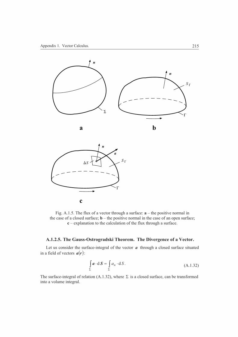
Appendix 1. Vector Calculus. 215
Fig. A.1.5. The flux of a vector through a surface: a – the positive normal inthe case of a closed surface; b – the positive normal in the case of an open surface;
c – explanation to the calculation of the flux through a surface.
A.1.2.5. The Gauss-Ostrogradski Theorem. The Divergence of a Vector.
Let us consider the surface-integral of the vector a through a closed surface situatedin a field of vectors ( )ra :
.dd ∫∫ΣΣ
⋅=⋅ SanSa (A.1.32)
The surface-integral of relation (A.1.32), where Σ is a closed surface, can be transformedinto a volume integral.
Σ
a b
c
n
n
n
a
Γ
Γ
S Γ
S Γ∆S

General Theory of the Electromagnetic Field216
Fig. A.1.6. The flux of a vector field through a parallelepiped surface.
The transformation relation represents the GAUSS-OSTROGRADSKI theorem (formula).Let us consider this transformation for a right infinitely small parallelepiped of surface
v . A field of vectors raa is considered. We shall calculate the surface-integral ofthe normal component of vector a over the surface v . The surface-integral will becalculated for the six faces of the parallelepiped with reference to Fig. A.1.6.
We shall denote by 0x , 0y , 0z the co-ordinates of the centre of the parallelepiped.Firstly, we consider the pair of faces perpendicular to the Ox - axis indicated by theordinal numbers 1 and 2. The quantity 000 ,, zyxa represents the vector a at the centreof the parallelepiped. The flux of the vector a through the surface 2 is:
,,,21
00022 zyzyxxaSa xx (A.1.33 a)
where the quantity xa2 is the mean value (average) of the component along the Ox - axisof the vector na on the face with the ordinal number 2, or the value at its middle.
The flux of the vector a through the face 1 is:
,,,21
00011 zyzyxxaSa xx (A.1.33 b)
where the quantity xa1 is the mean (average) value of the component along the Ox - axisof the vector na on the face with the ordinal number 1, or the value at its middle.
The total flux through the faces 1 and 2 is:
x
yy
O
z
x
z
M x y z( , , )
nn
a
0 0 0
Appendix 1. Vector Calculus. 217
,,,2
1,,
2
1000000 zyzyxxazyxxa xx (A.1.33 c)
and this sum, established with a precision up to small quantities of the third order, isequal to:
,0
21 zyxx
ax(A.1.33 d)
where the index 0 shows that the derivative is calculated at the centre of theparallelepiped.
For the pairs of faces perpendicular to the Oy and Oz axes, and indicated by theordinal numbers 3, 4, and 5, 6, respectively, the following sums of fluxes are obtained:
zyxy
ax
043 (A.1.33 e)
and
zyxz
ax
065 . (A.1.33 f)
Summing up, side by side, the preceding expressions, the total flux is obtained:
.d zyxz
a
y
a
x
aSa zyx
n
v
(A.1.34)
The sum within parentheses is called the divergence of the vector a or the divergenceof a and is denoted:
.divz
a
y
a
x
a zyxa (A.1.35)
The volume element will be denoted by:
.dddd zyxv (A.1.36)
With this symbol, the expression of the flux through the surface of an infinitely smallrectangular parallelepiped can be written:
.ddivd va (A.1.37)
We shall consider a domain of volume V bounded by any closed surface . Thisdomain can be decomposed by three sets of parallel planes, perpendicular to each other,in a set of rectangular infinitely small parallelepipeds. The marginal volume elementsneighbouring the surface are not in general of parallelepiped form. However, by a veryfine decomposition, it is possible to make the marginal elements to coincide with therequired precision with the surface . Calculating the flux of the vector a through the

General Theory of the Electromagnetic Field218
surface of each parallelepiped inside the surface and adding up, side by side, theobtained expressions, it follows:
,ddivddivd vv
VVV
aa (A.1.38)
the summation is extended over all volume elements, and namely over their surfaces.In the sum
V
d , the flux of vectors through each internal surface occurs twice,
namely the first time in the calculation of the flux through the surface of theparallelepiped situated on one side of this face, and the second time, in the calculation ofthe flux through the surface of the parallelepiped situated on the other side of this face.Since the positive normal of the considered face belonging to the first parallelepiped is ofopposite direction with regard to the positive normal of the same face belonging to thesecond parallelepiped, the fluxes through this surface are of opposite sign. Therefore, allthe terms of the sum above, which refer to the internal faces, cancel each other and thesum reduces to the sum of fluxes of vectors a only through the marginal surfaces of theparallelepipeds that coincide with the elements of the surface .
Hence:
.ddivd v
V
aSa (A.1.39)
For the relation (A.1.39) to be valid, the vector function must be continuous anddifferentiable at all the points of the domain V .
The relation (A.1.39) expresses the Gauss-Ostrogradski theorem and can be enouncedas follows: The flux of a vector a through any closed surface is equal to the volumeintegral of the divergence of the same vector over the volume bounded by this closedsurface.
If the surface is so small that at all points of its inside the quantity adiv may beassumed as constant, then, in relation (A.1.39) the quantity adiv can be placed before theintegral sign.
Hence:
,div va (A.1.40)
where the quantity v represents the volume of the domain V . It results that:
,
d
limdiv0 v
v
v
Sa
a(A.1.41)
and this expression can be considered as the definition of the divergence of a vector.From expression (A.1.41), it results that adiv does not depend on the choice of thesystem of co-ordinates.
The divergence of a vector can be expressed also in other systems of co-ordinates [12,tome I, p. 44].

Appendix 1. Vector Calculus. 219
A.1.2.6. The Line-integral of a Vector along a Curve. Circulation.
Let us consider the line-integral around an open curve C or a closed curve situatedin a field of vectors ra . The curve will be decomposed into very small line elements
l the direction of which coincide with the travelling sense considered as positive of thecurve. We shall express the scalar product of each element ld and the vector a at thecorresponding point:
.dd lalla (A.1.42)
The limit of the sum of the products of relation (A.1.42) along the curve is called theline-integral of the vector a along the curve C :
,ddC
l
C
lala (A.1.43)
where la is the component of the vector a along the direction of ld .The line-integral of the vector a along the curve C is referred to as the circulation of
vector a along that curve. That curve may be an open curve or a closed one [52, p. 138],[54, p. 123].
A.1.2.7. The Stokes Theorem. The Curl of a Vector.
Let us consider the line-integral of the vector a around a closed curve situated in afield of vectors ra :
.dd lalla (A.1.44)
The line-integral of relation (A.1.44), where is a closed curve, can be transformedinto a surface-integral. The transformation relation represents the STOKES theorem.
Let us consider this transformation for an infinitely small rectangle. A field of vectorsraa is considered. We shall calculate the line-integral of the vector a along the
contour of a rectangle, perpendicular to the Oz - axis, hence in the plane xOy , like in Fig.A.1.7. We have to calculate the line-integral decomposed for the four sides of therectangle with reference to Fig. A.1.7.
The travelling sense along the curve has been chosen associated, according to theright-handed screw rule, with the positive direction of the Oz - axis, hence, in the figure,the counter-clockwise sense.
We shall denote by 0x , 0y , 0z the co-ordinates of the centre of the rectangle.
The quantity 000 ,, zyxa represents the vector a at the centre of the rectangle. Theline-integral of the vector a along the side 1 is:
,,2
1, 00011 xzyyxaaC xx li (A.1.45 a)

General Theory of the Electromagnetic Field220
Fig. A.1.7. Circulation of a vector around a curve of a rectangle.
where the quantity xa1 is the mean value of the component along the Ox - axis of thevector a on the side having the ordinal number 1, or the value at its middle.
The line-integral along the side 3 is:
,,21, 00033 xzyyxaaC xx li (A.1.45 b)
where the quantity xa3 is the mean value of the component along the Ox - axis of thevector a on the side having the ordinal number 3, or the the value at its middle.
The line-integral along the sides 1 and 3 is:
,,21,,
21, 00000031 xzyyxazyyxaCC xx (A.1.45 c)
and after expanding in a series, it results that the sum including the small quantities of thesecond order, is equal to:
,0
31 yxy
aCC x (A.1.45 d)
where the index zero denotes that the derivative is calculated at the centre of therectangle.
The line-integral along the sides 2 and 4 is:
x
O x
a
1
z
y
3
24M (x y z, , )
y
A B
CD
0 0 0

Appendix 1. Vector Calculus. 221
.0
42 xyx
aCC
y(A.1.45 e)
By summing up, side by side, the relations established above, the following expressionof the integral is obtained:
.0
yxy
a
x
aC xy
(A.1.45 f)
It can be added that the quantity Cd is not a total differential of C . We consider theface having the normal n parallel with the Oz - axis. Denoting the area of the rectangleby yxSzd , i.e., after passing to limit, it follows:
.dd zxy
Sy
a
x
aCOz lan (A.1.46 a)
Analogously, for rectangles perpendicular to the other two axes, the followingrelations are obtained:
,dd xyz S
z
a
y
aCOx lan (A.1.46 b)
.dd yzx S
x
a
z
aCOy lan (A.1.46 c)
The combinations of the derivatives of the components of the vector a of expressions(A.1.46 a, b, c) are considered to be the components of a vector called curl or rotational ofthe vector a or curl of a and denoted acurl .
In this case, it follows:
,curlz
a
y
a yzxa (A.1.47 a)
,curlx
a
z
a zxya (A.1.47 b)
.curly
a
x
axy
za (A.1.47 c)
The vector acurl can be put in the form of a symbolic determinant:
General Theory of the Electromagnetic Field222
.curl
zyx aaa
zyx
kji
a (A.1.48)
By the aid of the symbol (A.1.48), the expressions (A.1.46 a, b, c) can be written inthe form:
,dcurld SaC (A.1.49)
where the unit vector n of the vector Sd is the positive normal to the surface Sd ,associated with the travelling direction along the contour of the surface, according to theright-handed screw rule. Making successively the vector n parallel with the axes Ox ,Oy , Oz , the expressions (A.1.46 a, b, c) are obtained. Hence, for a rectangle in each ofthe three positions, relation (A.1.49) is valid.
A simply connected surface bounded by a closed curve is considered. Let us take threesets of parallel planes, each plane of a set is parallel to one plane of the three planes of thethree-orthogonal rectilinear system of co-ordinates. The planes of each set are distancedby the steps x , y , z , respectively. If only the planes nearest the surface areconsidered, a surface constituted only by rectangles will be obtained. If the steps are verysmall and tend to zero, the surface constituted by rectangles tends to the given surface.
But for each rectangle of the surface formed by rectangles, relation (A.1.49) is valid.The relation (A.1.49) will be written for each rectangle, and these relations will besummed up, side by side. At each margin of two neighbouring rectangles, the commonside will be travelled twice in opposite directions, like in Fig. A.1.8, so that the sum
la d will contain the two terms of the form:
B
A
la d and ,dA
B
la (A.1.50)
the sum of which is zero. Hence, the sum la d becomes equal to the sum of termscorresponding only to the external boundary of the surface, hence to the integral of thevector a along the contour of the surface. It follows:
.dcurldS
C Sala (A.1.51)
For the relation (A.1.51) to be valid, the vector function a must be continuous anddifferentiable at all the points of the surface S . Relation (A.1.51) expresses the theoremof transformation of a line-integral into a surface-integral, called Stokes theorem that canbe enounced as follows: The circulation of an arbitrary vector a along a closed curveis equal to the flux of the curl of this vector through the surface S bounded by the curve
.From relation (A.1.51), it follows that in the case in which S is a closed surface:

Appendix 1. Vector Calculus. 223
Fig. A.1.8. The travelling of a vectoralong the elements of an open
surface bounded by a curve of any form.
S
,0dcurl Sa (A.1.52)
because if S is a closed surface, the contour reduces to a point and:
.0d la (A.1.53)
In the case in which S is a surface small enough for to be considered plane, and forall its points the quantity acurl to remain constant, the quantity acurl may be broughtout of the integral sign. Hence:
,curl SaC (A.1.54)
where S represents the area of the surface S .In this case, relation (A.1.54) can be written:
,curl SC na (A.1.55)
where the quantity nacurl is the component of the vector a along the positive normal
to the surface S . Therefore:
.
d
limcurl0 SS
n
la
a(A.1.56)
From expression (A.1.56), it results that the vector acurl does not depend on thechoice of the system of co-ordinates, hence it is an invariant with respect to the system ofco-ordinates.
The curl of a vector can also be expressed in various types of systems of co-ordinates[12, tome I, p. 44].

General Theory of the Electromagnetic Field224
A.1.2.8. Nabla Operator. Hamilton Operator.
Previously it has been established that the gradient of a scalar function is a vector
oriented along the direction of the maximal increase of the function , with themagnitude equal to the derivative of the function along this direction. Among the varioussymbols of the gradient, one of the most utilized is .
The sign is read nabla or also del and it denotes a differential operator. With thissymbol, it is possible to write:
.zyx
kji (A.1.57)
From this expression, it can be seen that the operator can be considered as adifferential operator:
,zyx
kji (A.1.58)
that, being applied to the scalar function , gives the quantity grad . This operator canbe considered as a symbolic vector and it is also called the Hamilton operator.
A.1.2.9. The Derivative of a Vector along a Direction
Let us consider an arbitrary point rM in a field of vectors ra like in Fig. A.1.9.
Let srM be another point in the same vector field. In particular cases, the arbitrarypoint M can be considered on a curve the tangent of which at the point M has thedirection of the unit vector s , but it is not a condition. The unit vector s can be written:
.zyx sss kjis (A.1.59 a)
Fig. A.1.9. Explanation to thecalculation of the derivative of a vector
along a given direction.
O
a a r
s
( r ) ( )+
r +r
MM'
s
s
s
Appendix 1. Vector Calculus. 225
The limit of the ratio
s
rasra(A.1.59 b)
as 0s , is termed the derivative of the vector a along the direction of the unit vectors at the considered point M and is denoted:
.lim0 ss s
rasraa
(A.1.60)
Introducing the co-ordinates, we obtain:
.,,,,
lim0 s
zyxzzyyxx
s s
aaa(A.1.61 a)
By expanding in a series, and retaining only the small quantities of the first order, weobtain:
,d
d
d
d
d
d
s
z
zs
y
ys
x
xs
aaaa(A.1.61 b)
where
.d
d;
d
d;
d
dksjsis zyx s
s
zs
s
ys
s
x(A.1.61 c)
It follows that:
.zyxs
aks
ajs
ais
a(A.1.62)
Since we have 1s , the last relation is the scalar product as of the following
scalar operator:
zyxksjsiss (A.1.63 a)
and the vector a , and gives just s
a, so that the symbol as appears as justified.
Now, the more general case is examined, in which in expression s instead of theunit vector s , any vector v will be considered. Hence, the scalar operator obtained byperforming the scalar product of the arbitrary vector vsv and the symbolic vector ,is:

General Theory of the Electromagnetic Field226
.
,
v
zv
yv
xv
sv
ksjsisv(A.1.63 b)
Therefore:
,zyx
va
ksa
jsa
isav (A.1.63 c)
.;; kskvjsjvisiv vvvvvv zyx (A.1.63 d)
Hence:
zv
yv
xv zyx
aaaav (A.1.64)
or, in another compact form:
.
,
v
sv
sv
aav
(A.1.64 a)
In the case in which 1v , the operation above represents the derivative of the vectora with respect to the direction of the vector v . Hence, the expression av representsthe derivative of the vector a with respect to the direction of the vector v multiplied bythe modulus of the last vector.
A.1.2.10. Expressing the Divergence and the Curl of a Vectorby Means of the Nabla Operator
The divergence can also been expressed, formally, as the scalar product of thesymbolic vector by the vector a :
.zyx aaa kjia (A.1.65 a)
By performing this product according the formula of the scalar product of two vectors
,zzyyxx abababab (A.1.65 b)
and putting
,;;z
by
bx
b zyx (A.1.65 c)
it follows:
Appendix 1. Vector Calculus. 227
.z
a
y
a
x
a zyxa (A.1.66)
Analogously, the curl of a vector can be considered as the vector product of thesymbolic vector by the vector a :
,curl
zyx aaa
zyx
kji
aa (A.1.67 a)
.curly
a
x
a
x
a
z
a
z
a
y
a xyzxyz kjiaa (A.1.67 b)
A.1.2.11. Differential Operations by the Nabla Operator
The differential operator:
zyxkji (A.1.68)
is constituted by three partial derivatives relatively to the axes of co-ordinates. In the casein which it is applied to a product, the operation is the same as in the case of thecalculation of the derivative of a product. The first term will be calculated considering thefirst factor as variable and the other factors as constants. The second term will becalculated considering the second factor as variable and the other factors as constants, etc.In the case of the application of the operator , always when confusions could appear,all the vectors that will be considered momentary to be constant, will be denoted by theindex c (constant). The computing method by the operator can be explained asfollows. All vectors occurring in the expression under consideration, excepting oneconsidered as variable are supposed as being constant. Then, the expression will betransformed, so that, all constant vectors may be arranged before the operator , and theone considered as variable, after this operator. If from the point of view of VectorAlgebra two variants are valid, the variant giving a result different from zero will be kept.
Sometimes, the derivation of the relations by using the operator , due to its formalcharacter, could be considered as being rather a mnemonic rule than a rigorous proof. Forthis reason, the usage of the symbolic operator requires certain precaution.

General Theory of the Electromagnetic Field228
Derivatives of Products
1.
.gradgradgrad
;grad cccc
(A.1.69)
2.
.graddivdiv
;div
aaa
aaaaaa cccc
(A.1.70)
3.
.gradcurlcurl
;
curl
aaa
aa
aa
aaaa
cc
cc
cc
(A.1.71)
4.
.curlcurldiv
;
div
baabb
abbaabab
abba
babababa
cccc
cc
cc
(A.1.72)
5. ;grad cc babababa (A.1.73 a)
but
.
;
BCABCABAC
BACCABCBA
(A.1.73 b)
By substituting
;;; bBaAC c (A.1.73 c)
it follows
.bababa ccc (A.1.73 d)
Analogously:
.ababba ccc (A.1.73 e)
Therefore:
.curlcurlgrad
;
abbaabbaba
abbaabbaba
(A.1.74)
Appendix 1. Vector Calculus. 229
6. ,curl cc babababa (A.1.75 a)
but
.CABCABBACCABCBA (A.1.75 b)
By substituting
;;; bCaBA c (A.1.75 c)
it follows:
.bababa ccc (A.1.75 d)
Analogously:
.ababba ccc (A.1.75 e)
Therefore:
.divdivcurl
;
baababbaba
abbaabbaba
(A.1.76)
The utilization of the nabla operator simplifies much the calculation of the derivatives
of the first, second and higher orders of scalar and vector quantities. In this way,important relations of higher orders can be obtained as follows.
Analogously to the relations of Vector Algebra as 2bbb , for b , thefollowing relations can be obtained:
;graddiv 2 (A.1.77 a)
but
.2
zzyyxx(A.1.77 b)
Therefore:
.graddiv2
2
2
2
2
22
zyx (A.1.78)
By applying relation (A.1.78) for r
1, where r is the modulus of the position
vector, it follows:
1.
222
2 ;01
zyxr
r (A.1.79)
General Theory of the Electromagnetic Field230
and
.r
rr
(A.1.80)
2..divgrad
z
a
y
a
x
a
zyx
zyxkjiaa (A.1.81)
3..
2
2
2
2
2
22
zyx
aaaaa (A.1.82)
4..grad
22222
zyx(A.1.83)
Analogously to relations of Vector Algebra:
5. abbabbabbabbbb ,0,0
and for b , the following relations are obtained:
;0gradcurl (A.1.84)
;0curldiv aa (A.1.85)
.divgrad 2aaaaa (A.1.86)
All relations above can be verified by direct calculation, using the co-ordinates of athree-orthogonal rectilinear system of reference.
A.1.2.12. Integral Transformations Using the Nabla Operator
1º Scalar integral relations. GREEN theorem. In relation (A.1.39) that expresses theGauss-Ostrogradski theorem:
,dddiv Saa v
V
the following substitution will be performed:
,grada (A.1.87 a)
where and are two arbitrary scalars and:
.b (A.1.87 b)
It follows:
.graddivdiv cccc bbbba (A.1.87 c)

Appendix 1. Vector Calculus. 231
Hence:
.gradgradgraddivdiv a (A.1.87 d)
Therefore:
.dgradddddiv 2 Svv
VV
nSaa (A.1.87 e)
But:
.gradn
n (A.1.87 f)
It follows:
.dd2 Sn
v
V(A.1.88)
Analogously, replacing the quantities and by each other, it follows:
.dd2 Sn
v
V(A.1.89)
By subtracting the two last relations, it follows:
.dd22 Snn
v
V(A.1.90)
The relations (A.1.88), (A.1.89) and (A.1.90) are the three forms of the Greentheorem.
2º Vector integral relations. The following volume integral will be calculated:
.dcurl v
V
a (A.1.91 a)
For this purpose, this integral will be multiplied by any constant vector c :
.dcurldcurl vv
V
acac (A.1.91 b)
According to formula (A.1.72), taking into account that const,c it follows:
.curldiv acca (A.1.91 c)

General Theory of the Electromagnetic Field232
The two last equations yield:
.dcurlddiv vv
VV
acca (A.1.91 d)
The last relation, taking into account relation (A.1.39), becomes:
,dcurld v
V
acSca (A.1.91 e)
and hence:
.dcurld vS
V
acnca (A.1.91 f)
The last relation, taking into account relation (A.1.9 a), becomes:
.dcurld vS
V
acanc
Taking into account that the last relation holds whatever the constant vector c wouldbe, it follows:
.dcurld vS
V
aan (A.1.92)
A.1.2.13. Substantial Derivative of a Scalar with Respect to Time
In a reference frame supposed to be at rest, let us consider any point rM moving at
velocity rv relatively to this frame, and the scalar function tf ,r that is depending onthe point M and that is varying with time.
In various cases, it is necessary to calculate the derivative of the form:
,,d
dtMf
t(A.1.93)
in another reference frame that is moving at the same velocity rv as the point M andhence with respect to which the point is at rest. In cases of interest, the point M is fixedto the surrounding substance that is moving together with the point M . For this reasonthe considered derivative is referred to as substantial derivative.
The variation with time of the function f in the moving reference frame isdetermined by two causes: a. The modification of the position of the point M in thereference frame at rest; b. The variation with time of the function at each point of thereference frame at rest.
The derivative is obtained from the expression:
.,,,,,,1
lim,d
d0
tzyxfttzzyyxxft
tMft t
(A.1.94)

Appendix 1. Vector Calculus. 233
It follows:
tt
fz
z
fy
y
fx
x
f
ttzyxf
t t d
d
d
d
d
d
d
d1lim,,,
d
d0
(A.1.95)
or
,d
d
d
d
d
d
d
d,,,
d
d
t
fv
z
fv
y
fv
x
ftzyxf
trzryrx (A.1.96)
where the components of the velocity at which the point zyxM ,, is moving relatively
to the reference frame at rest have been denoted rxv , ryv , rzv . Therefore:
.gradd
d,
d
df
t
ftf
trvr (A.1.97)
A.1.2.14. Substantial Derivative of a Volume Integral of a ScalarFunction with Respect to Time
In various cases, it is necessary to calculate the derivative of the form:
,dd
d
V
vft (A.1.98)
where tftMff ,, r is a scalar function with space, i.e., depends on the moving
point M . In the most general case, when both the function f and the volume V arevarying with time, the derivative of the given form is referred to as substantial derivativewith respect to time. The reason of the usage of the term substantial has been mentionedabove.
As in the preceding Sub-section, the derivative can be decomposed as follows:
.dd
dd
d
dd
d
d
constconstVf
VV
V
vft
vft
vft
(A.1.99)
By differentiating the first term of the right-hand side, it follows:
,dgrad
dd
d
d
d
d
dd
d
d
const
V
r
VVV
vft
f
vt
z
z
f
t
y
y
f
t
x
x
f
t
fvf
t
v
(A.1.100 a)

General Theory of the Electromagnetic Field234
where rv represents the velocity of both the moving point and the substance relatively tothe reference frame at rest.
The second term of the right-hand side will be differentiated considering the variationof the volume. The final value of the volume after the time interval t is:
,d tVV r Sv (A.1.100 b)
where Sv dr represents the volume described by the surface element Sd in the unit oftime.
Using the relation (A.1.39) for rva , the last relation becomes:
.ddivdV
rr vvSv (A.1.100 c)
Relations (A.1.100 b) and (A.1.100 c) yield:
,ddiv vtVV rv (A.1.100 d)
.VVV (A.1.100 e)
It follows:
.ddivlimdd
dd
d
d0
const V V
rt
fV
vft
VVfv
tfvf
tv (A.1.100 f)
By substituting expressions (A.1.100 a) and (A.1.100 f) in relation (A.1.99), itfollows:
.ddivgraddd
d
V
rr
V
vfft
fvf
tvv
(A.1.101)
Finally, it follows:
.ddivdd
dvf
t
fvf
tV
r
V
v(A.1.102)

Appendix 1. Vector Calculus. 235
A.1.2.15. Derivative with Respect to Time of the Flux through a MovingOpen Surface
Let us calculate the derivative with respect to time of the flux of a vector t,rG
through a simply connected open surface bounded by any closed simple curve , whenthe surface S is moving relatively to a reference frame considered at rest.
The velocity of any point of the surface S or of the curve will be denoted by rv
and may have various values at different points. It is assumed that at any point of theconsidered domain, the vector t,rG is differentiable with respect to time and with theco-ordinates of the reference frame. The corresponding flux is:
.d,S
t SrG (A.1.103)
The variation with time of the quantity will be determined by two causes: a. Thevariation with time of the vector t,rG , at each point of the reference frame at rest;
b. The modification with time of the position and sizes of the surface S . After an
interval of time t , the surface S occupies another position and becomes the surface
S , as can be seen in Fig. A.1.10.The derivative with respect to time of the flux is given by the expression:
.,d,1
limd,d
d
d
d0
SSt
S
tttt
ttt
rGSrGSrG (A.1.104)
The first integral of the last side, if only the small quantities of the first order are kept, canbe expanded in the form:
.d,
d,d,SSS
t
ttttt S
rGSrGSrG
(A.1.105 a)
In the last integral of the right-hand side, which is a small quantity of the first order, theinfluence of the variation of S will be neglected producing a small quantity of higherorder. It results that:
.d,d,1
lim
d,
d,d
d
0SS
t
SS
ttt
t
tt
t
SrGSrG
SrG
SrG
(A.1.105 b)
It follows that the derivative with respect to time of the flux of a vector through anopen surface that is moving relatively to a reference frame (supposed at rest) is given bythe sum of two terms: a – the derivative of the flux supposing the open surface at rest
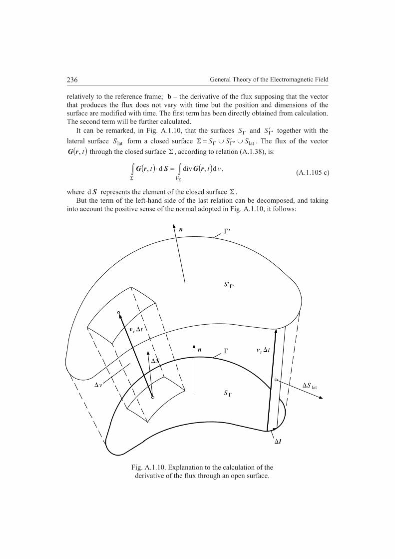
General Theory of the Electromagnetic Field236
relatively to the reference frame; b – the derivative of the flux supposing that the vectorthat produces the flux does not vary with time but the position and dimensions of thesurface are modified with time. The first term has been directly obtained from calculation.The second term will be further calculated.
It can be remarked, in Fig. A.1.10, that the surfaces S and S together with the
lateral surface latS form a closed surface latSSS . The flux of the vector
t,rG through the closed surface , according to relation (A.1.38), is:
,d,divd, vtt
V
rGSrG (A.1.105 c)
where Sd represents the element of the closed surface .But the term of the left-hand side of the last relation can be decomposed, and taking
into account the positive sense of the normal adopted in Fig. A.1.10, it follows:
Fig. A.1.10. Explanation to the calculation of thederivative of the flux through an open surface.
S
v
v r t
S
rv t
l
n
n
S
S' '
'
lat

Appendix 1. Vector Calculus. 237
( ) ( ) ( ) ( ) . d , d , d , d , lat
lat ∫ ∫ ∫ ∫ Σ ′
+ ⋅ + ⋅ − = ⋅ Γ ′ Γ S S S
t t t t S r G S r G S r G S r G (A.1.105 d)
The element of the surface lat S , with the symbols of Fig. A.1.10, is:
. lat t r ∆ × ∆ = ∆ v l S (A.1.105 e)
The volume element of the domain Σ V , with the symbols of Fig. A.1.10, is:
( ) . S v ∆ ⋅ ∆ = ∆ t v r (A.1.105 f)
From relations (A.1.105 d) and (A.1.105 e), it follows:
( ) ( ) ( )
. d ,
d , d , d , ∫ ∫ ∫
Γ
Σ ′
× ⋅ ∆ −
− ⋅ + ⋅ − = ⋅ Γ ′ Γ
l v r G
S r G S r G S r G
r
S S
t t
t t t
(A.1.105 g)
From relations (A.1.105 c), (A.1.105 f), (A.1.105 g), it follows:
( ) ( ) ( ) ( )
( ) ( ) ( ) . d ,
d , div d , d , ∫ ∫ ∫
Γ
′
× ⋅ ∆
+ ⋅ ∆ = ⋅ − ⋅ Γ Γ Γ ′
l v r G
S r G v S r G S r G
r
S S r
S
t t
t t t t
(A.1.105 h)
Relations (A.1.105 b) and (A.1.105 h) yield:
( ) ( ) ( ) [ ]
( )
∫
Γ
Γ
⋅ +
+ ⋅ × − ⋅ ∂
∂ = ⋅
Γ Γ
. d , div
d , d , d , d d
S r G v
l r G v S r G S r G
t
t t
t t t
r
S r
S (A.1.106)
+

General Theory of the Electromagnetic Field238
APPENDIX 2
EXPRESSIONS OF THE DIFFERENTIAL OPERATORS INCURVILINEAR CO-ORDINATES
A.2.1. GENERAL CONSIDERATIONS
In applications, besides the three-orthogonal rectilinear system of co-ordinates, othersystems of co-ordinates are also of importance. Further on, the expressions of thedifferential operators for various systems of co-ordinates will be recalled [12, tome I,p. 44].
In the three-orthogonal system with rectilinear axes, the position of any point isdetermined by the distances of that point to the planes determined by the axes of co-ordinates.
Hence, any point MMM zyxM ,, can be considered as the intersection of the planes:
,,, MMM zzyyxx (A.2.1 a, b, c)
parallel with the planes yOz , zOx , xOy , respectively.The intersection of planes consty and constz represents the line of variation of
the quantity x . The line 0y ; 0z represents the line of co-ordinate x . Analogously,the lines of the co-ordinates y and z can be obtained. The three lines obtained in thisway are straight lines.
The quantities zyx ,, represent the co-ordinates of the three-orthogonal system of co-ordinates with rectilinear axes.
Generally, if the following three sets of surfaces are considered:
,,,,,,,,, 332211 CzyxxCzyxxCzyxx (A.2.2 a, b, c)
and if various values are given to the constants 321 ,, CCC , it can be considered thateach point M of the space is determined by a set of three values corresponding to thethree constants.
The intersection of the surfaces 22 Cx and 33 Cx represents the line of variation
of the quantity 1x . The line 02x ; 03x represents the line of the co-ordinate 1x .
Analogously, it is possible to obtain the lines of variation of the quantities 2x and 3x .In the general case, the lines of variation are not straight lines but curvilinear ones. For
this reason, in the general case, a system of curvilinear co-ordinates is obtained as inFig. A.2.1.
The quantities 321 ,, xxx represent the co-ordinates of a curvilinear system of co-ordinates.

General Theory of the Electromagnetic Field240
Fig. A.2.1. Curvilinear system ofco-ordinates.
Between the co-ordinates 321 ,, xxx of a curvilinear system of co-ordinates and theco-ordinates zyx ,, of a three-orthogonal rectilinear system of co-ordinates, there are thefollowing relations:
.,,;,,
;,,;,,
;,,;,,
321333
321222
321111
xxxzzyxfx
xxxyzyxfx
xxxxzyxfx
(A.2.3 a, . . ., f)
The position of a point M can be defined by the corresponding position vector r .At any point 321 ,, xxxM of the curvilinear system of co-ordinates, it is possible to
construct three fundamental vectors 1e , 2e , 3e , tangent to the lines of co-ordinates
321 ,, xxx , and each of them having the length equal to unity. Hence, the threefundamental vectors above are unit vectors. The three vectors form a trihedron that canhave a different position at each point. In addition, it should be noted that the unit vectors
1e , 2e , 3e , tangent to the lines of co-ordinates, are oriented in the sense in which the co-
ordinates 321 ,, xxx increase.The chief difference between the curvilinear system of co-ordinates and the rectilinear
system of co-ordinates resides as mentioned in the fact that, in the case of a curvilinearsystem, the directions of vectors 1e , 2e , 3e depend on the point at which these vectorsare taken.
The expression of a vector in this system of curvilinear co-ordinates is:
.332211 aaa eeea (A.2.4)
Further on, we shall consider only those systems of curvilinear co-ordinates for whichthe three fundamental vectors are perpendicular to each other. These are called
O
e
e
e
3
2
1
x
x
x 2
3
1

Appendix 2. Expressions of the Differential Operators in Curvilinear Co-ordinates. 241
rectangular or orthogonal systems of curvilinear co-ordinates. In this work, only systemsof co-ordinates the fundamental vectors of which form a right trihedron are used. Theyare termed right-angled systems of co-ordinates.
The displacement of a point 321 ,, xxxM at a variation 1d x , of the co-ordinate 1x ,
the other two co-ordinates being constant, is 1d s .
Analogously, the following variations will be obtained: 2d s at a variation 2d x and
3d s at a variation 3d x . The expressions for the length of the element of arc, the area ofthe surface elements and the volume of an element, taking into account that the system isorthogonal, and neglecting the small quantities of higher order, are:
.dddd 23
22
21
2 ssss (A.2.5)
.ddd
,ddd
,ddd
213
132
321
ssS
ssS
ssS
(A.2.6 a, b, c)
.dddd 321 sssV (A.2.7)
We shall take into account that the partial derivative of the position vector r withrespect to the co-ordinate 1x (the co-ordinates 2x and 3x remain constant) is:
,111
hx
er
(A.2.8)
where:
.11
hx
r(A.2.9)
It follows:
,ddd 11111
11 xhxx
s er
e (A.2.10)
hence:
.dd 111 xhs (A.2.11)
Analogously, it is possible to obtain the corresponding expressions of 2d s and 3d s .The following expressions are obtained:
.dddd 23
23
22
22
21
21
2 xhxhxhs (A.2.12)
;ddd;ddd;ddd 212131313232321 xxhhSxxhhSxxhhS (A.2.13 a, b, c)

General Theory of the Electromagnetic Field242
;dddd 321321 xxxhhhV (A.2.14)
;i
ix
hr
(A.2.15)
.222
iiii
x
z
x
y
x
xh (A.2.16)
The quantities of the form ih are called LAMÉ coefficients.We shall express the differential operators taking into account the relations above. The
gradient of a scalar function 321 ,, xxx has the expression:
.111
grad33
322
211
1xhxhxh
eee (A.2.17)
The divergence of a vector 321 ,, xxxa has the expression:
.1
div 2133
1322
3211321
hhax
hhax
hhaxhhh
a (A.2.18)
The curl of a vector 321 ,, xxxa has the expression:
.1
11curl
112
22121
3
331
11313
2223
33232
1
hax
haxhh
hax
haxhh
hax
haxhh
e
eea
(A.2.19)
The Laplace operator applied to a scalar function, 2 , has the expression:
.1
33
21
322
13
211
32
1321
2
xh
hh
xxh
hh
xxh
hh
xhhh
(A.2.20)
A.2.2. FORMULAE FOR THREE-ORTHOGONAL RECTILINEAR,CYLINDRICAL AND SPHERICAL CO-ORDINATES
Further on, the following three-orthogonal systems of co-ordinates will be considered:Three-orthogonal rectilinear system of co-ordinates, cylindrical system of co-ordinates,spherical polar system of co-ordinates.

Appendix 2. Expressions of the Differential Operators in Curvilinear Co-ordinates. 243
Fig. A.2.2. System of cylindricalco-ordinates.
Fig. A.2.3. System of spherical polarco-ordinates.
Besides these, also other systems of three-orthogonal systems are used, for instancethe elliptical system of co-ordinates.
For a three-orthogonal system of co-ordinates with rectilinear axes, it follows:
.1;1;1
;dddd
;;;
321
2222
321
hhh
zyxs
zxyxxx
(A.2.21 a, . . ., g)
For a cylindrical system of co-ordinates (Fig. A.2.2), it follows:
.1;;1
;dddd
;;sin;cos
;;;
321
2222
3
321
hhh
zs
xzyx
zxxx
(A.2.22 a, . . ., j)
For a spherical system of co-ordinates (Fig. A.2.3), it follows:
N
M
O
r
x
y
z
N
M
O
r
x
y
z
General Theory of the Electromagnetic Field244
( ) ( ) ( ).sin;;1
;dsinddd
;cos;sinsin;cossin
;;;
321
2222
321
θ===ϕθ+θ+=
θ=ϕθ=ϕθ=ϕ=θ==
rhrhh
rrrs
rzryrx
xxrx
(A.2.23 a, . . ., j)
The relations of differential operators in cylindrical co-ordinates:
( ) ( ) ( ) .grad;1
grad;gradz
z ∂Φ∂
=Φϕ∂Φ∂
⋅ρ
=Φρ∂Φ∂
=Φ ϕρ (A.2.24 a, b, c)
( ) .11
divz
aaa z
∂∂
+ϕ∂
∂⋅
ρ+ρ
ρ∂∂
⋅ρ
= ϕρa (A.2.25)
( ) ( ) ( ) ( ) .11
curl;curl;1
curlϕ∂
∂⋅
ρ−ρ
ρ∂∂
⋅ρ
=ρ∂
∂−
∂
∂=
∂
∂−
ϕ∂∂⋅
ρ= ρ
ϕρ
ϕϕ
ρ
aa
a
z
a
z
aaz
zz aaa
(A.2.26)
.11
2
2
2
2
22
z∂
Φ∂+
ϕ∂
Φ∂⋅
ρ+⎟⎟
⎠
⎞⎜⎜⎝
⎛ρ∂Φ∂
ρρ∂∂
⋅ρ
=Φ∇ (A.2.27)
The relations of differential operators in spherical co-ordinates:
( ) ( ) ( ) .sin
1grad;
1grad;grad
ϕ∂Φ∂
⋅θ
=Φθ∂Φ∂
⋅=Φ∂Φ∂
=Φ ϕθrrr
r
(A.2.28 a, b, c)
( ) ( ) .sinsin
11div 2
2 ⎥⎦
⎤⎢⎣
⎡
ϕ∂
∂+θ
θ∂∂
θ+
∂∂
⋅= ϕθ
aa
rar
rrra (A.2.29)
( ) ( )
( ) ( )
( ) ( ) .1
curl
;1
sin
1curl
;sinsin
1curl
⎥⎦
⎤⎢⎣
⎡θ∂
∂−
∂∂
=
∂∂
⋅−ϕ∂
∂⋅
θ=
⎥⎦
⎤⎢⎣
⎡ϕ∂
∂−θ
θ∂∂
θ=
θϕ
ϕθ
θϕ
r
r
r
aar
rr
arrr
a
r
aa
r
a
a
a
(A.2.30 a, b, c)
.sin
11sin
sin
112
2
2222
22
ϕ∂
Φ∂⋅
θ⋅+⎟⎟
⎠
⎞⎜⎜⎝
⎛θ
θ∂Φ∂
θ∂∂
⋅θ
+⎟⎟⎠
⎞⎜⎜⎝
⎛∂Φ∂
∂∂
⋅=Φ∇rrr
rrr
(A.2.31)
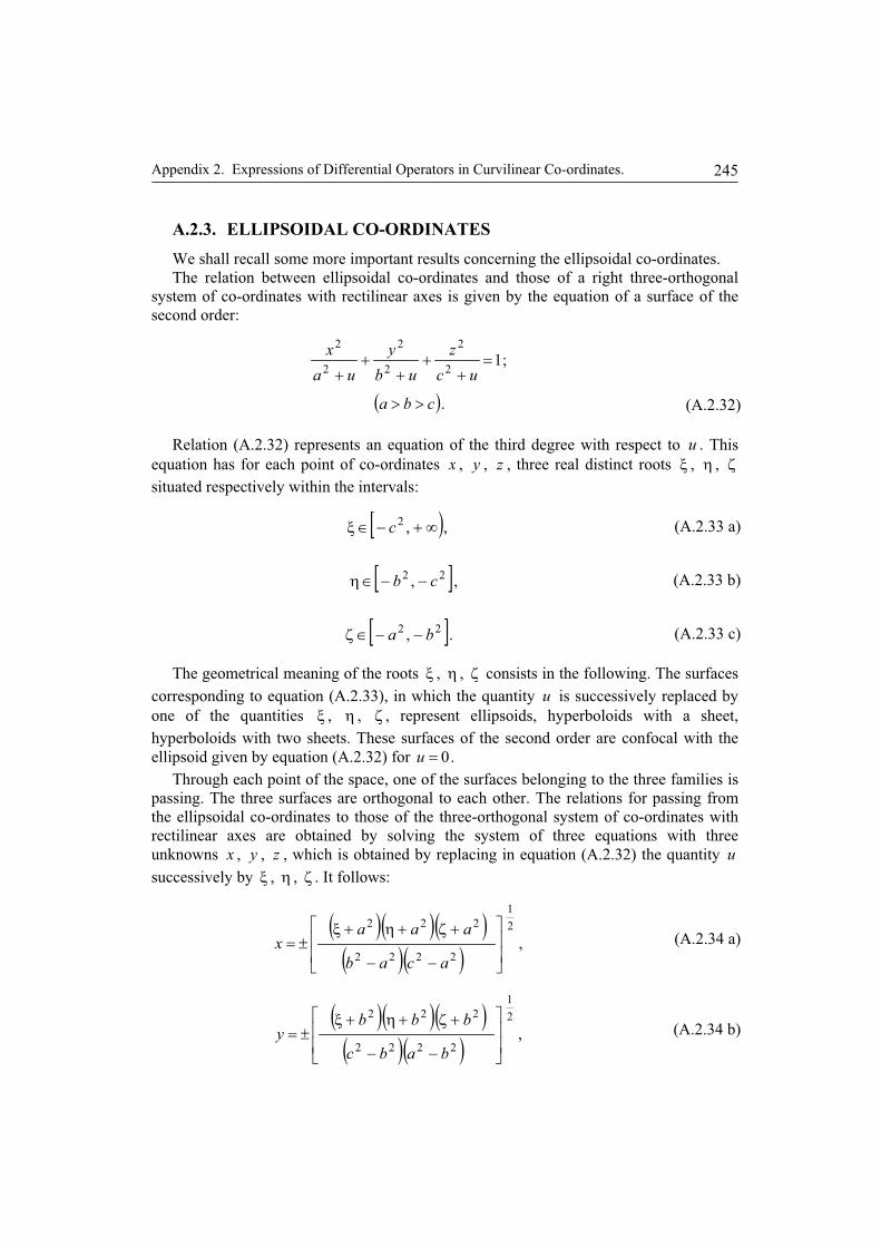
Appendix 2. Expressions of Differential Operators in Curvilinear Co-ordinates. 245
A.2.3. ELLIPSOIDAL CO-ORDINATES
We shall recall some more important results concerning the ellipsoidal co-ordinates.The relation between ellipsoidal co-ordinates and those of a right three-orthogonal
system of co-ordinates with rectilinear axes is given by the equation of a surface of thesecond order:
;12
2
2
2
2
2
=+
++
++ uc
z
ub
y
ua
x
( ).cba >> (A.2.32)
Relation (A.2.32) represents an equation of the third degree with respect to u . Thisequation has for each point of co-ordinates x , y , z , three real distinct roots ξ , η , ζsituated respectively within the intervals:
[ ),,2 ∞+−∈ξ c (A.2.33 a)
[ ],, 22 cb −−∈η (A.2.33 b)
[ ]., 22 ba −−∈ζ (A.2.33 c)
The geometrical meaning of the roots ξ , η , ζ consists in the following. The surfacescorresponding to equation (A.2.33), in which the quantity u is successively replaced byone of the quantities ξ , η , ζ , represent ellipsoids, hyperboloids with a sheet,hyperboloids with two sheets. These surfaces of the second order are confocal with theellipsoid given by equation (A.2.32) for .0=u
Through each point of the space, one of the surfaces belonging to the three families ispassing. The three surfaces are orthogonal to each other. The relations for passing fromthe ellipsoidal co-ordinates to those of the three-orthogonal system of co-ordinates withrectilinear axes are obtained by solving the system of three equations with threeunknowns x , y , z , which is obtained by replacing in equation (A.2.32) the quantity u
successively by ξ , η , ζ . It follows:
( )( )( )( )( )
,2
1
2222
222
⎥⎥
⎦
⎤
⎢⎢
⎣
⎡
−−
+ζ+η+ξ±=
acab
aaax (A.2.34 a)
( )( )( )( )( )
,2
1
2222
222
⎥⎥
⎦
⎤
⎢⎢
⎣
⎡
−−
+ζ+η+ξ±=
babc
bbby (A.2.34 b)

General Theory of the Electromagnetic Field246
( )( )( )( )( )
.2
1
2222
222
⎥⎥
⎦
⎤
⎢⎢
⎣
⎡
−−
+ζ+η+ξ±=
cbca
cccz (A.2.34 c)
To each point of co-ordinates x , y , z , of the three-orthogonal system of co-ordinates
with rectilinear axes, there corresponds a point of co-ordinates ξ , η , ζ , in the ellipsoidalsystem of co-ordinates.
The length element expressed in ellipsoidal co-ordinates is:
( ) ( ) ( ) ,dddd 2222222 ζ+η+ξ= ζηξ hhhs (A.2.35)
where the following symbols have been used:
( )( );
2 ξξ
ζ−ξη−ξ=
Rh
( )( );
2 ηη
ξ−ηζ−η=
Rh
( )( );
2 ζζ
η−ζξ−ζ=
Rh (A.2.36 a, b, c)
( ) ( ) ( )[ ] ;21
222cubuauRu +++++=
( ).,, ζηξ=u (A.2.37)
The expression of the quantity V2∇ in ellipsoidal co-ordinates is:
( )( )( ) ( ) ( )
( ) .
1
2
1
2
⎥⎦
⎤⎟⎟⎠
⎞⎜⎜⎝
⎛ζ∂
∂ζ∂∂
η−ξ+
⎢⎣
⎡+⎟⎟
⎠
⎞⎜⎜⎝
⎛η∂
∂η∂∂
ξ−ζ+⎟⎟⎠
⎞⎜⎜⎝
⎛ξ∂
∂ξ∂∂
ζ−ηζ−ηξ−ζη−ξ
=∇
ζζ
ηηξξ
VRR
VRR
VRRV
(A.2.38)
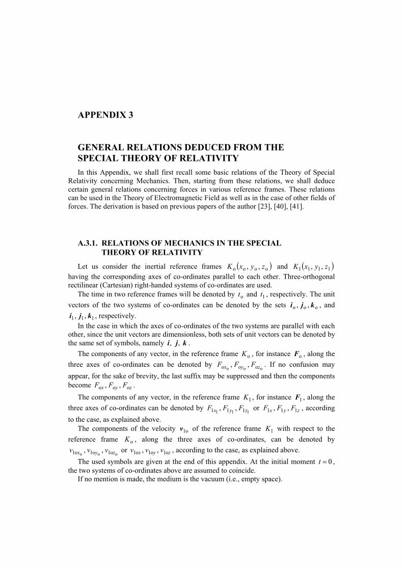
APPENDIX 3
GENERAL RELATIONS DEDUCED FROM THESPECIAL THEORY OF RELATIVITY
In this Appendix, we shall first recall some basic relations of the Theory of SpecialRelativity concerning Mechanics. Then, starting from these relations, we shall deducecertain general relations concerning forces in various reference frames. These relationscan be used in the Theory of Electromagnetic Field as well as in the case of other fields offorces. The derivation is based on previous papers of the author [23], [40], [41].
A.3.1. RELATIONS OF MECHANICS IN THE SPECIALTHEORY OF RELATIVITY
Let us consider the inertial reference frames oooo ,, zyxK and 1111 ,, zyxK
having the corresponding axes of co-ordinates parallel to each other. Three-orthogonalrectilinear (Cartesian) right-handed systems of co-ordinates are used.
The time in two reference frames will be denoted by ot and 1t , respectively. The unit
vectors of the two systems of co-ordinates can be denoted by the sets ooo ,, kji , and
111 ,, kji , respectively.In the case in which the axes of co-ordinates of the two systems are parallel with each
other, since the unit vectors are dimensionless, both sets of unit vectors can be denoted bythe same set of symbols, namely kji ,, .
The components of any vector, in the reference frame oK , for instance oF , along the
three axes of co-ordinates can be denoted by ooo ooo ,, zyx FFF . If no confusion may
appear, for the sake of brevity, the last suffix may be suppressed and then the componentsbecome zyx FFF ooo ,, .
The components of any vector, in the reference frame 1K , for instance 1F , along the
three axes of co-ordinates can be denoted by 111 111 ,, zyx FFF or zyx FFF 111 ,, , according
to the case, as explained above.The components of the velocity o1v of the reference frame 1K with respect to the
reference frame oK , along the three axes of co-ordinates, can be denoted by
ooo o1o1o1 ,, zyx vvv or zyx vvv o1o1o1 ,, , according to the case, as explained above.
The used symbols are given at the end of this appendix. At the initial moment 0t ,the two systems of co-ordinates above are assumed to coincide.
If no mention is made, the medium is the vacuum (i.e., empty space).

General Theory of the Electromagnetic Field248
In order to facilitate the understanding of the treatment, firstly we shall recall therelations of Mechanics in the Special Theory of Relativity, brought in a convenient form,in accordance with the following treatment.
We consider the relation in the Special Theory of Relativity as being obtained directly,hence without resorting to the equations of Electromagnetism.
A.3.1.1. General Relations of Mechanics in the Special Theory ofRelativity
Between the quantities of Mechanics given in the list of symbols at the end of thisappendix, the relations below have been established and will be given using three-dimensional vectors (Fig. A.3.1). For the sake of simplicity, we denote 11 rr A , oo rr P .
If no mention is made, we shall also assume xvv o1o1o1 iiv . The quantities in the
reference frame 1K , expressed in terms of the quantities of the reference frame oK , are:
,12o1
o1oo1oo1o1oo1o1
vtt
vvrvvrr (A.3.1)
,;1
1 o1o1
2o1
o1c
v(A.3.1 a, b)
,12o1
o1oo1o1o1
v
vlvll (A.3.2)
,1
1 o1oo12o1
o1oo11 vSvSSv
(A.3.3)
,oo11 VV (A.3.4)
,2
oo1oo11
ctt
rv(A.3.5)
,1
1
1 o12o1
2o1o1o2
o1o2o1
o1
o1o2o1
o1o221 v
vvv (A.3.6 a)
.1
1
1 o12o1
2o1o121
o121o1
o1
o112o1
o121o2 v
vvv (A.3.6 b)
The last two relations can be brought in a form sometimes suitable in applications, forinstance the latter:
,111 o112o1
o121
o112o1
o121
o112
o121o2
vvkvvjvviv zyx (A.3.6 c)

Appendix 3. General Relations Deduced from the Special Theory of Relativity. 249
Fig. A.3.1. The systems of co-ordinates oooo ,, zyxK , 1111 ,, zyxK ,and a position vector.
,
1
11
3
2o1o23
o1
o22o2o1
o12o1
o1o2o1o1o22
o1o2o1
21
c
cvc
vv
vavv
avavv
a (A.3.7)
,12
o1o2o11 m
cm
vv
(A.3.8)
,;
1
o2
2
2
0 vu
c
u
mm
(A.3.9)
where the quantity m is the relativistic mass in the reference frame oK of a material
point moving at the velocity o2vu relative to this reference frame, whereas 1m is the
relativistic mass in the reference frame 1K , and 0m is the mass of the material point at
rest in oK .
A x , y , z1 A 1 A 1 A( )1z
y
1x
y
z
1y
O
tx v1 x
x
( y,x )z,P
x
1v
o o o
o
o
oo
o
ov1 t ox
oK K1
o
o o o
o
r A1
O1
1o t ov
r o P
r PA
r P1

General Theory of the Electromagnetic Field250
,1
1
1
1
1
1
o1o2
oo1o22o12
o1
o1o
o1o2o1
o1o
o1o2o1
o1o2o11
Fvvv
vFFF
cv
(A.3.10)
,1
1
1
1
1
1
o121
1o1212o12
o1
o11
o121o1
o11
o112o1
o121o1o
Fvvv
vFFF
cv
(A.3.11)
.;; 1221
o2o2
o1o1
ccc
vvv(A.3.11 a, b, c)
We assume that there is a certain inertial reference frame oK that has the following
property. The force acting in this reference frame upon a particle p that is moving at any
velocity const,pnv relative to the reference frame nK is independent of the velocity
pnv .
For instance, in the given reference frame 1K , the force 1
F can be independent of the
velocity 21v . Such an example occurs in the case in which there is a point-like electric
charge 1q at rest in the reference frame, and 1F is the force exerted upon any point-like
charge 2q moving at the velocity 21v relatively to the reference frame 1K . The value of
a force in the reference frame nK and for instance in the reference frame 1K in theexample above is referred to as proper value of the force.
The forces in any reference frame, say 1K , can be expressed in terms of the forces in acertain reference frame, say, by means of a relation of the type (A.3.10).
At the same time, we assume that all the geometrical elements (lines, surfaces) havetheir proper dimensions (sizes) in the reference frame nK . The geometrical dimensions
(sizes) in the reference frame nK can be expressed in terms of the geometricaldimensions (sizes) of any other reference frame by means of the relations above (A.3.2)and (A.3.3).
With the usual denominations, the geometrical dimensions are contravariantquantities, whereas the forces are covariant quantities. When writing various relations, itis useful to take into account this remark.
It is possible to express the relation between the differential operators when passingfrom one reference frame to another [23, Vol. I, p. 504]. These operators concerngradient, divergence, curl and derivative with respect to time.
Remark. In the case in which o1v is not of the form xv o1i , any vector oooo ,, zyxr
or 1111 ,, zyxr can be decomposed into three components: One parallel to the direction
of o1v and the other two components perpendicular to the direction of o1v , chosen so
that, together with the component parallel to the direction of o1v , they form a Cartesian
right-handed reference frame. Then, the transformation relations can be applied for eachcomponent. Therefore, the relations of Sub-section A.3.1.1 subsist.
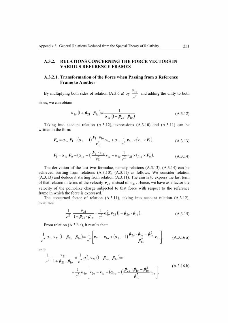
Appendix 3. General Relations Deduced from the Special Theory of Relativity. 251
A.3.2. RELATIONS CONCERNING THE FORCE VECTORS INVARIOUS REFERENCE FRAMES
A.3.2.1. Transformation of the Force when Passing from a ReferenceFrame to Another
By multiplying both sides of relation (A.3.6 a) by 2
o1
c
v and adding the unity to both
sides, we can obtain:
.1
11
o1o2o1o121o1 (A.3.12)
Taking into account relation (A.3.12), expressions (A.3.10) and (A.3.11) can bewritten in the form:
,1
1 1o1o22o1o12o1
o11o11o1o Fvvv
vFFF
cv(A.3.13)
.1
1 oo1212o1o12o1
o1oo1oo11 Fvvv
vFFF
cv(A.3.14)
The derivation of the last two formulae, namely relations (A.3.13), (A.3.14) can beachieved starting from relations (A.3.10), (A.3.11) as follows. We consider relation(A.3.13) and deduce it starting from relation (A.3.11). The aim is to express the last termof that relation in terms of the velocity o2v instead of 12v . Hence, we have as a factor thevelocity of the point-like charge subjected to that force with respect to the referenceframe in which the force is expressed.
The concerned factor of relation (A.3.11), taking into account relation (A.3.12),becomes:
.11
1
1o1o221
2o12
o121
212
vv
cc(A.3.15)
From relation (A.3.6 a), it results that:
,11
11
o12o1
2o1o1o2
o1o1o22o1o221o12vvvv
cc(A.3.16 a)
and:
,11
11
1
1
o12o1
2o1o1o2
o1o1o2o12
o1o2212o12
o121
212
vvv
vv
c
cc(A.3.16 b)
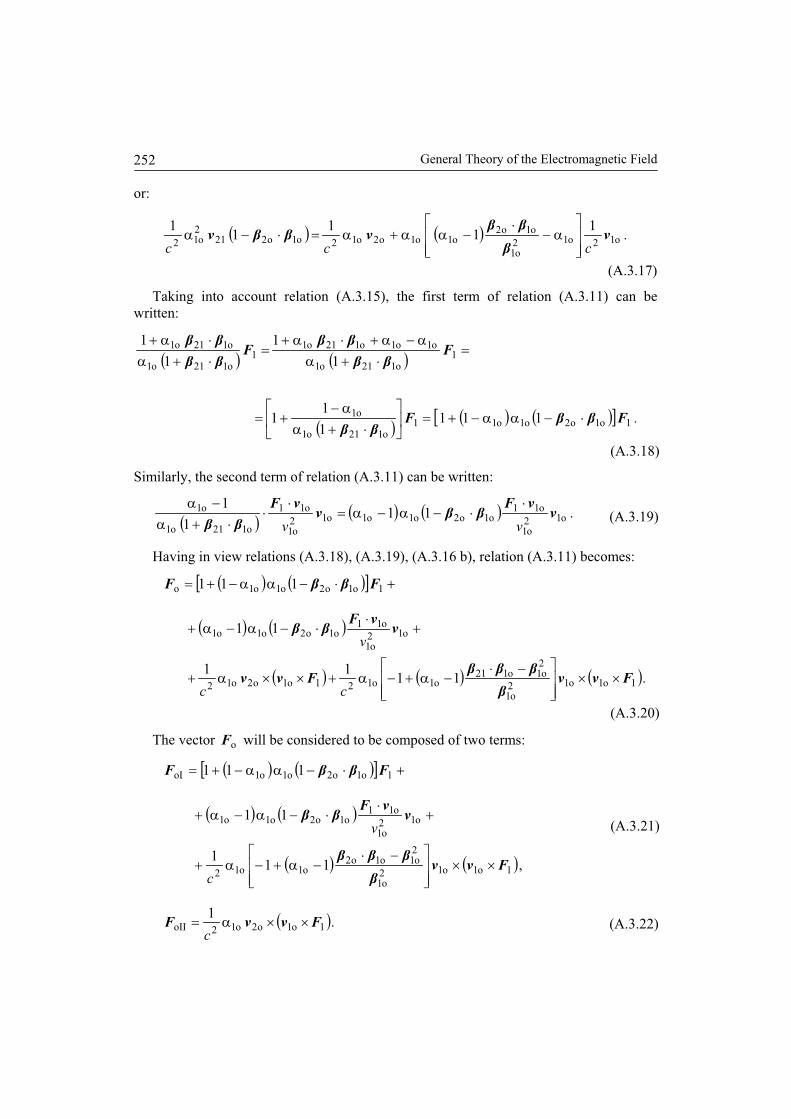
General Theory of the Electromagnetic Field252
or:
.1
11
11
o12o12o1
o1o2o1o1o2o12o1o221
2o12
vvvccc
(A.3.17)
Taking into account relation (A.3.15), the first term of relation (A.3.11) can bewritten:
.1111
11
1
1
1
1
1o1o2o1o11o112o1
o1
1o112o1
o1o1o121o11
o112o1
o121o1
FF
FF
(A.3.18)
Similarly, the second term of relation (A.3.11) can be written:
.111
1o12
o1
o11o1o2o1o1o12
o1
o11
o121o1
o1 vvF
vvF
vv(A.3.19)
Having in view relations (A.3.18), (A.3.19), (A.3.16 b), relation (A.3.11) becomes:
.1111
11
111
1o1o12o1
2o1o121
o1o121o1o2o12
o12o1
o11o1o2o1o1
1o1o2o1o1o
FvvFvv
vvF
FF
cc
v
(A.3.20)
The vector oF will be considered to be composed of two terms:
,111
11
111
1o1o12o1
2o1o1o2
o1o12
o12o1
o11o1o2o1o1
1o1o2o1o1oI
Fvv
vvF
FF
c
v (A.3.21)
.1
1o1o2o12oII FvvFc
(A.3.22)

Appendix 3. General Relations Deduced from the Special Theory of Relativity. 253
At this stage, the calculations can be shortened as follows. Let us assume xv o1o1 iv .In this case, along the Ox - axis, from relation (A.3.21), we obtain:
.111
11
111
12o111o1o12
o1
2o1o1o2
o1o12
o12o1
o11o1o2o1o1
1o1o2o1o1oI
xxxxxx
x
x
xx
xx
FvFFvvc
vv
vF
FF
(A.3.23)
Similarly, along the Oy - axis, from relation (A.3.21), we obtain:
,1
1111
111
111
1o112o1
2o1
2o1o1
12o12
o1
2o1o1o2
o1o1o1o1o2o1o1
2o112
o1
2o1o1o2
o1o12
1o1o2o1o1oI
yy
y
xy
yy
FF
F
vFc
FF
(A.3.24)
since:
.11 2o1
2o1 (A.3.24 a)
Similarly, we obtain
.1o1oI zz FF (A.3.25)
Finally, we have:
,oIoIoIoI zyx FFF kjiF (A.3.26 a)
zyx FFF 1o11o11oI kjiF (A.3.26 b)
or in compact form:
.1 o12o1
o11o11o1oI v
v
vFFF (A.3.27)
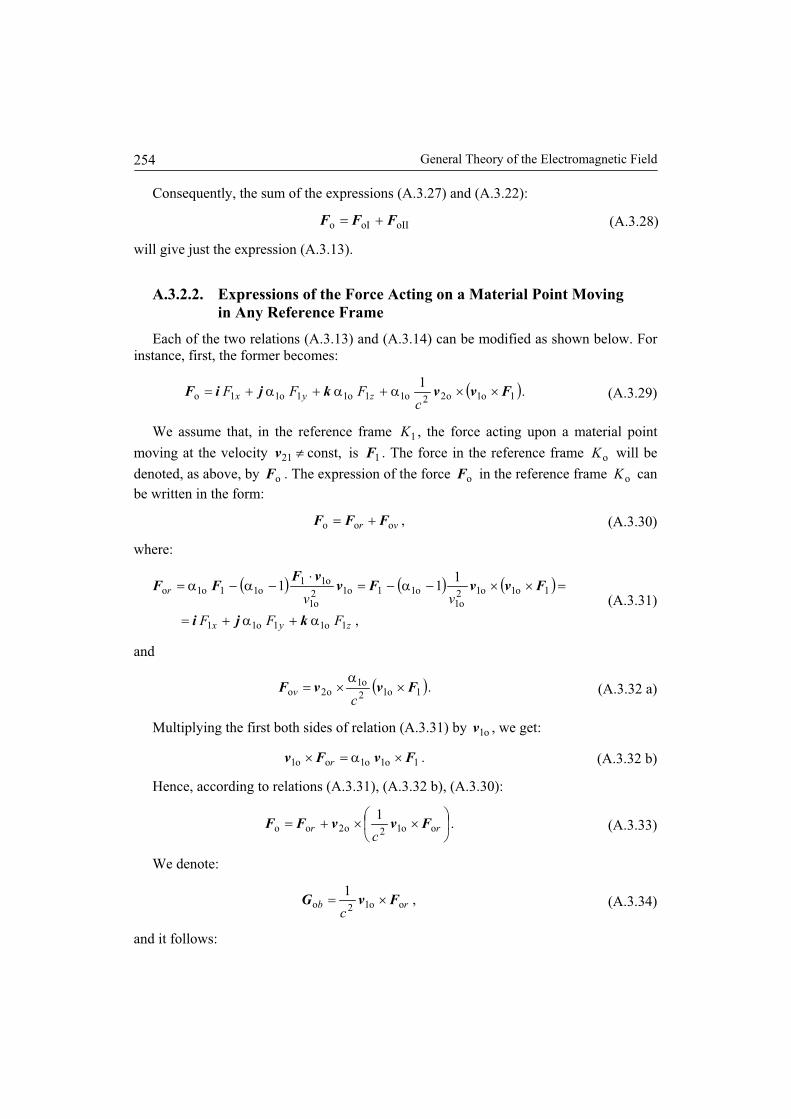
General Theory of the Electromagnetic Field254
Consequently, the sum of the expressions (A.3.27) and (A.3.22):
oIIoIo FFF (A.3.28)
will give just the expression (A.3.13).
A.3.2.2. Expressions of the Force Acting on a Material Point Movingin Any Reference Frame
Each of the two relations (A.3.13) and (A.3.14) can be modified as shown below. Forinstance, first, the former becomes:
.1
1o1o22o11o11o11o FvvkjiFc
FFF zyx (A.3.29)
We assume that, in the reference frame 1K , the force acting upon a material point
moving at the velocity const,21v is 1F . The force in the reference frame oK will be
denoted, as above, by oF . The expression of the force oF in the reference frame oK canbe written in the form:
,ooo vr FFF (A.3.30)
where:
,
111
1o11o11
1o1o12o1
o11o12o1
o11o11o1o
zyx
r
FFF
vv
kji
FvvFvvF
FF(A.3.31)
and
.1o12o1
o2o FvvFc
v (A.3.32 a)
Multiplying the first both sides of relation (A.3.31) by o1v , we get:
.1o1o1oo1 FvFv r (A.3.32 b)
Hence, according to relations (A.3.31), (A.3.32 b), (A.3.30):
.1
oo12o2oo rrc
FvvFF (A.3.33)
We denote:
,1
oo12o rbc
FvG (A.3.34)
and it follows:
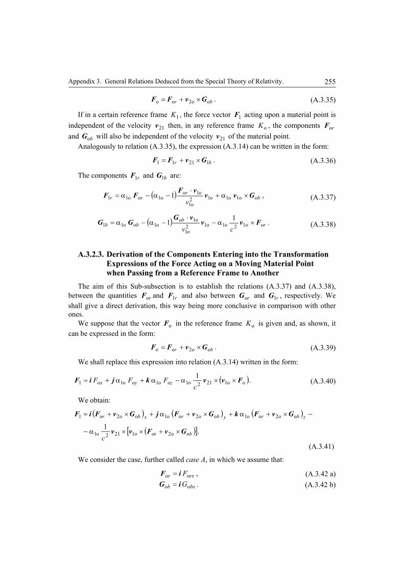
Appendix 3. General Relations Deduced from the Special Theory of Relativity. 255
.oo2oo br GvFF (A.3.35)
If in a certain reference frame 1K , the force vector 1F acting upon a material point is
independent of the velocity 21v then, in any reference frame oK , the components roF
and boG will also be independent of the velocity 12v of the material point.Analogously to relation (A.3.35), the expression (A.3.14) can be written in the form:
.11211 br GvFF (A.3.36)
The components r1F and b1G are:
,1 o1oo1o12o1
o1oo1oo11 b
rrr
vGvv
vFFF (A.3.37)
.1
1 o1o2o1o12o1
o1oo1oo11 r
bbb
cvFvv
vGGG (A.3.38)
A.3.2.3. Derivation of the Components Entering into the TransformationExpressions of the Force Acting on a Moving Material Pointwhen Passing from a Reference Frame to Another
The aim of this Sub-subsection is to establish the relations (A.3.37) and (A.3.38),between the quantities roF and r1F and also between roG and r1G , respectively. Weshall give a direct derivation, this way being more conclusive in comparison with otherones.
We suppose that the vector oF in the reference frame oK is given and, as shown, itcan be expressed in the form:
.oo2oo br GvFF (A.3.39)
We shall replace this expression into relation (A.3.14) written in the form:
.1
oo1212o1oo1oo1o1 FvvkjiFc
FFF zyx (A.3.40)
We obtain:
.1
oo2oro1212o1
oo2oo1oo2oo1oo2o1
b
zbrybrxbr
cGvFvv
GvFkGvFjGvFiF
(A.3.41)
We consider the case, further called case A, in which we assume that:
,oo rxr FiF (A.3.42 a).oo bxb GiG (A.3.42 b)
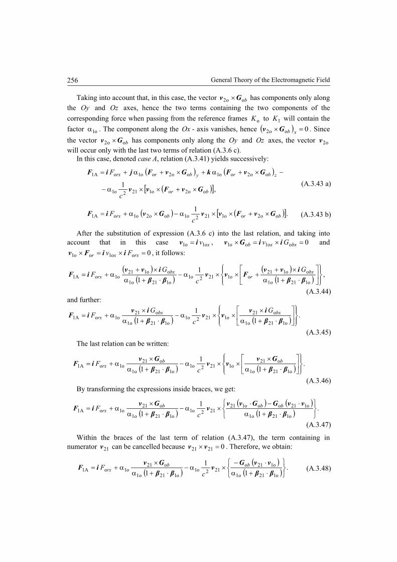
General Theory of the Electromagnetic Field256
Taking into account that, in this case, the vector boo2 Gv has components only alongthe Oy and Oz axes, hence the two terms containing the two components of the
corresponding force when passing from the reference frames oK to 1K will contain the
factor o1 . The component along the Ox - axis vanishes, hence 0oo2 xbGv . Since
the vector boo2 Gv has components only along the Oy and Oz axes, the vector o2v
will occur only with the last two terms of relation (A.3.6 c).In this case, denoted case A, relation (A.3.41) yields successively:
,1
oo2oo1212o1
oo2oo1oo2oo1o1A
br
zbrybrrx
c
F
GvFvv
GvFkGvFjiF
(A.3.43 a)
.1
oo2oo1212o1oo2o1o1A brbrxc
F GvFvvGviF (A.3.43 b)
After the substitution of expression (A.3.6 c) into the last relation, and taking intoaccount that in this case xv o1o1 iv , 0oo1oo1 bxxb Gv iiGv and
0oo1oo1 rxxr Fv iiFv , it follows:
,1
1
1 o1211o
oo121oo1212o1
o1211o
oo121o1o1A
ivvFvv
ivviF bx
rbx
rx
G
c
GF
(A.3.44)and further:
.1
1
1 o1211o
o21o1212o1
o1211o
o21o1o1A
ivvv
iviF bxbx
rx
G
c
GF
(A.3.45)
The last relation can be written:
.1
1
1 o1211o
o21o1212o1
o1211o
o21o1o1A
Gvvv
GviF bb
rxc
F
(A.3.46)By transforming the expressions inside braces, we get:
.1
1
1 o1211o
o121ooo121212o1
o1211o
o21o1o1A
vvGGvvv
GviF bbb
rxc
F
(A.3.47)
Within the braces of the last term of relation (A.3.47), the term containing innumerator 21v can be cancelled because 02121 vv . Therefore, we obtain:
.1
1
1 o1211o
o121o212o1
o1211o
o21o1o1A
vvGv
GviF bb
rxc
F (A.3.48)
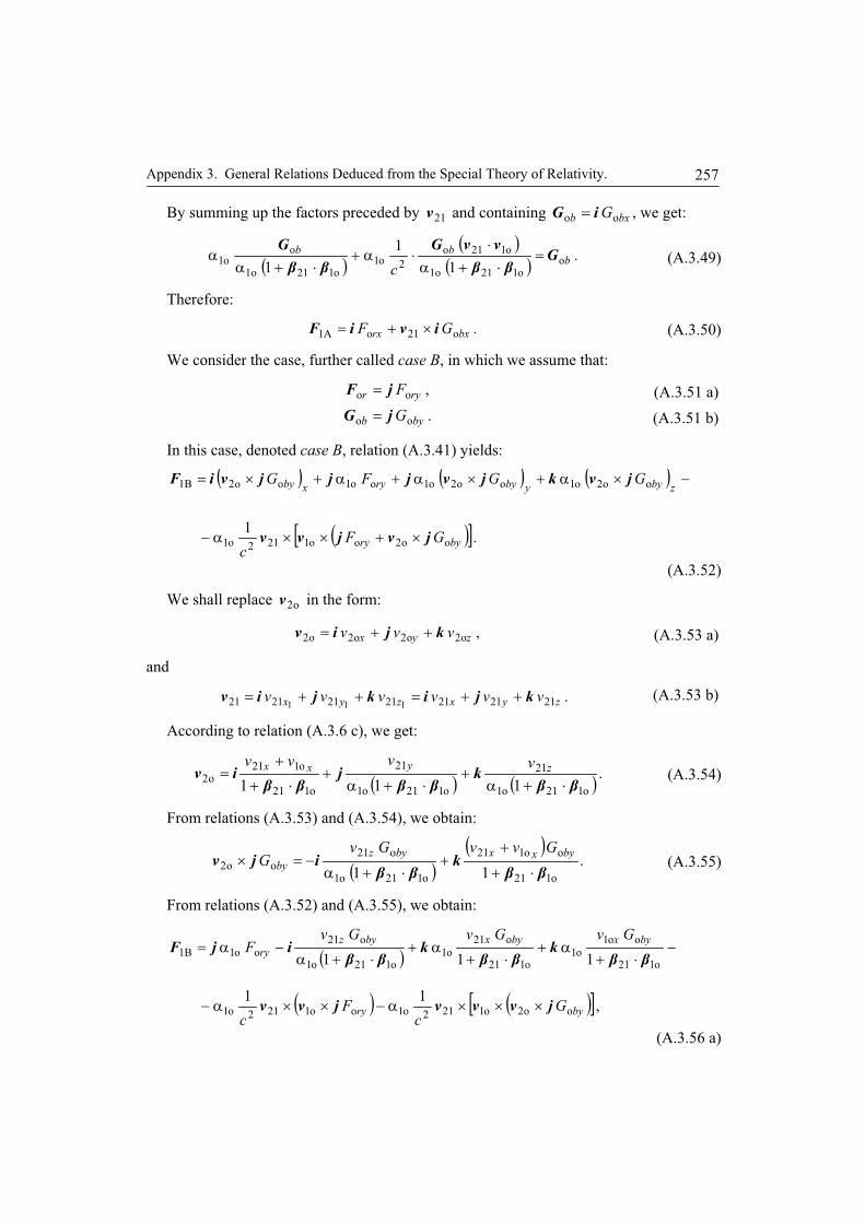
Appendix 3. General Relations Deduced from the Special Theory of Relativity. 257
By summing up the factors preceded by 21v and containing bxb Goo iG , we get:
.1
1
1 oo1211o
o121o2o1
o1211o
oo1 b
bb
cG
vvGG(A.3.49)
Therefore:
.o21o1A bxrx GF iviF (A.3.50)
We consider the case, further called case B, in which we assume that:
,oo ryr FjF (A.3.51 a)
.oo byb GjG (A.3.51 b)
In this case, denoted case B, relation (A.3.41) yields:
.1
oo2oo1212o1
oo2o1oo2o1oo1oo21B
byry
zbyybyryxby
GFc
GGFG
jvjvv
jvkjvjjjviF
(A.3.52)
We shall replace o2v in the form:
,o2o2o2o2 zyx vvv kjiv (A.3.53 a)
and
.12122112122112 111 zyxzyx vvvvvv kjikjiv (A.3.53 b)
According to relation (A.3.6 c), we get:
.111 o112o1
21
o112o1
21
o112
o121o2 kjiv zyxx vvvv
(A.3.54)
From relations (A.3.53) and (A.3.54), we obtain:
.11 o112
oo121
o112o1
o21oo2 kijv
byxxbyzby
GvvGvG (A.3.55)
From relations (A.3.52) and (A.3.55), we obtain:
,11
111
oo2o1212o1oo1212o1
o121
oo1o1
o121
o21o1
o121o1
o21oo11B
byry
byxbyxbyzry
Gc
Fc
GvGvGvF
jvvvjvv
kkijF
(A.3.56 a)

General Theory of the Electromagnetic Field258
and:
.11
1
1
111
oo121
o121
o121o1
21o1212o1
oo1212o1
o121
oo1o1
o121
o21o1
o121o1
o21oo11B
byxxz
ry
byxbyxbyzry
Gvvv
c
Fc
GvGvGvF
kivv
jvv
kkijF
(A.3.56 b)
By substituting in the last relation xv o1o1 iv , we obtain:
.1
1
1
111
oo121
o121o1212o1
oo1212o1
o121
oo1o1
o121
o21o1
o121o1
o21oo11B
byxx
x
ry
byxbyxbyzry
Gvv
vc
Fc
GvGvGvF
jv
jvv
kkijF
(A.3.57)
For obtaining the result in a compact form, we shall express the various terms asfollows.
1º The term having as coefficient the quantities i , byGo , zv21 .
The corresponding factor is:
,1
1
11
11
o1o121o1
2o1
2o1o121
2o1
o121
2o1o121
o1o121o1
(A.3.57 a)
since
.12o1
2o1
2o1
2º The term having as coefficient the quantities k , byGo , xv21 .
The corresponding factor is:
.11
1o1
o121
o121o1
o121o1 (A.3.57 b)

Appendix 3. General Relations Deduced from the Special Theory of Relativity. 259
3º The term having as coefficient the quantities k , byGo , xv o1 .
The corresponding factor is:
.11
1o1
o121
o121o1
o121o1 (A.3.57 c)
By replacing the terms corresponding to factors given by relations (A.3.57 a, b, c) intoexpression (A.3.57), it follows:
.
1
oo1o1o21o1
o21o1oo1212o1oo11B
byxbyx
byzryry
GvGv
GvFc
F
kk
ijvvjF(A.3.58)
By introducing the vector products, the last relation can be written in the form:
.1
oo12o1oo121oo1o1oo11B rybybyry Fc
GGF jvjvjvjF
(A.3.59)
Therefore:
.12111B br GvFF (A.3.60)
Similarly, we can obtain:
.1
oo12o1oo121oo1o1oo11C rzbzbzrz Fc
GGF kvkvkvkF
(A.3.61)
Hence:
.12111C br GvFF (A.3.62)
By summing up, side by side, the relations (A.3.50), (A.3.59), (A.3.61), it follows:
.1
oo12o1oo1oo1o21
oo1o1oo1oo1o1
rbzbybx
brzryrx
cGGG
FFF
Fvkjiv
GvkjiF
(A.3.63)
Therefore:
.12111 br GvFF (A.3.64)
By comparing relations (A.3.63) with (A.3.64), it follows that the quantities r1F and
b1G are expressed in terms of the quantities roF and boG just by the relations (A.3.37)and (A.3.38).

General Theory of the Electromagnetic Field260
A.3.3. INTEGRAL AND LOCAL FORMS OF RELATIONSCONTAINING THE VECTORS IN VARIOUS REFERENCEFRAMES
A.3.3.1. The Fluxes of Vectors roF and r1F through a Surface
We may consider as known the resultant force 1F in the reference frame 1K acting
upon a moving material point and we assume that it is independent of the velocity 21v .
Hence, according to relation (A.3.36), the vector b1G is zero.
We need to calculate the flux of the vectors roF and r1F through a given surface,
open or closed, in the reference frames oK and 1K , respectively. Firstly, we shall
calculate the flux in the reference frame 1K .
For obtaining the surface element 1S , we start from the quantity oS in the
reference frame oK where the flux has to be calculated. For calculating the vector roF ,
we start from the vector 1F in the reference frame 1K where the resultant force has beenconsidered. In this way, as we shall show immediately, the flux remains unchanged in thetwo reference frames. The conservation of the flux through a surface is equivalent withthe geometrical interpretation that the number of lines of field, through the consideredsurface, remains unchanged.
In the reference frame oK , we obtain the flux:
.oo SF r (A.3.65)
Taking into account relation (A.3.36) and 01bG of above, it results that r11 FF .
Hence, in the reference frame 1K , we obtain the flux:
.1
1 1o1oo12o1
o1o1o111 FvSvSFSFv
r (A.3.66)
But in the reference frame oK , as shown above, by relation (A.3.31), we have:
.1
1 o11o12o1
o11o1o vFvFFv
r (A.3.67)
Multiplying both sides of the last equation by oS , it follows:
.oo11 SFSF rr (A.3.68)
For a closed surface, we obtain:
,dd
o1
oo11 SFSF rr (A.3.69 a)
in integral form, and:

Appendix 3. General Relations Deduced from the Special Theory of Relativity. 261
,divdiv ooo111 rr FF (A.3.69 b)
in differential (local) form, respectively. The index of the operator div indicates thereference frame in which this operator has been calculated.
A.3.3.2. The Flux of the Vector boG through a Closed Surface
We need to calculate the fluxes of vectors boG given by relation (A.3.34) through a
given surface, a closed or open one, in the reference frame oK :
.1
11
11
o1o1o12
oo1o112o1
o11o1o12oo1o2oo
SFv
SvvFFvFvSSG
c
vccrb
(A.3.70)
Taking into account relation (A.3.3) and that 0o11o1 vFv , it follows:
.1
11
1
11
11
11o12
o1oo12o1
o1oo11o12
oo1o112o1
o11o1o12ooo12oo
SFv
vSvSFv
SvvFFvSFvSG
c
vc
vccrb
(A.3.71)
It follows:
,dcurl1
d1
d
11o
111o1211o12oo
V
b Vcc
FvSFvSG (A.3.72)
in integral form, and
,curl1
div 11o12ooo1 FvGc
b (A.3.73)
in differential (local) form. The indices of the operators div and curl indicate thereference frame in which these operators have been calculated.

General Theory of the Electromagnetic Field262
A.3.3.3. The Circulation of the Vector roF along a Closed Curve in theCase of a Field of Vectors with Central Symmetry
We need to calculate the circulation of the vector roF round a closed curve in the
reference frame oK . We consider the case of any field of forces with central symmetry in
the reference frame 1K . We also assume the same condition as at the beginning of Sub-
section A.3.3.1, and hence 01bG . As previously, we adopt the axes of the system of co-
ordinates in a convenient manner, namely so that the vector velocity o1v be parallel andof the same direction with the Ox - axis. The general expression of the forces in theconsidered case is:
,111 APAPf rrF (A.3.74)
where the position vector APAP rr1 has the origin at any point AAA zyxA 111 ,, , source
point, and the extremity at the point ooo ,, zyxP , observation or field point, at which the
mentioned force has to be calculated at any moment 1t in the reference frame 1K . Theposition vector can be expressed in the form:
,1o1o1oo1oo11 AAAxAP zzyyxtvx kjir (A.3.74 a)
or, generally, for any direction of o1v :
.1 12o1
o1oo1oo1o1oo1o1 AAP
vtt r
vvrvvrr (A.3.74 b)
We shall use the expression of the force (A.3.31) in the form:
.1o11o11o zyxr FFF kjiF (A.3.75)
The circulation of the vector roF round a closed curve is:
,dcurld
oo
ooooS
rr SFlF(A.3.76)
whereo
S is a simply connected open surface bounded by the curve o . It is assumed
that on the surfaceo
S the function 1o rF r is differentiable at each point. Taking into
account the relations (A.3.74), (3.75), (A.3.76), after performing the calculations ofcomponents of the curl applied to that function, we obtain:
.11
0curl oo12zoo12o
oo ryxrxr Fvc
Fvct
kjiF (A.3.77)
Hence, taking into account relation (A.3.34), we get:

Appendix 3. General Relations Deduced from the Special Theory of Relativity. 263
.1
curl oo
oo12o
oo brrtct
GFvF (A.3.78)
Since the operator ocurl and the time ot are invariant with respect to thetransformation for passing from one three-orthogonal rectilinear system of co-ordinates toanother three-orthogonal rectilinear system co-ordinates at rest relative to the first one, itfollows that relation (A.3.78) remains valid for any direction of the velocity o1v . Since
relations (A.3.77), (A.3.75), (A.3.74) are linear relatively to vectors roF , boG , 1r , itfollows that relation (A.3.78) is valid also in the case in which the right-hand side ofrelation (A.3.74) is a linear combination of terms of the same form. It follows:
,dd
oo
ooo
ooS
brt
SGlF (A.3.79)
in integral form, and
,curl oo
oo brt
GF (A.3.80)
in differential (local) form.It can be remarked the analogy of the two last relation with the expression of the law
of electromagnetic induction.
A.3.3.4. The Circulation of the Vector boG along a Closed Curve in theCase of a Field of Vectors with Central Symmetry
We need to calculate the circulation of the vector boG round (along) a closed curve in
the reference frame oK . We consider the case of a field of vectors of central symmetry in
the reference frame 1K and under the same conditions as in Sub-section A.3.3.1.
The circulation of the vector boG along any closed curve o is:
,dcurld
oo
oooooS
bb SGlG(A.3.81)
whereo
S is the open surface bounded by the curve o . Taking into account relation
(A.3.34), we can write:
.1
div11
curlcurl ooo12ooo12oo12ooo rrrbccc
FvFvFvG (A.3.82)
Taking into account relations (A.3.74), (A.3.75), after performing the calculations ofthe components of each vector, we shall obtain:

General Theory of the Electromagnetic Field264
.11
o
o2ooo12 tcc
rr
FFv (A.3.83)
Therefore, relation (A.3.82) becomes:
.1
div1
curl oo
2ooo12oo rrbtcc
FFvG (A.3.84)
The operator ocurl , the operator odiv , and the time ot are invariant with respect tothe transformation from one right-handed three-orthogonal rectilinear system of co-ordinates to another right-handed three-orthogonal rectilinear system of co-ordinates, atrest relative to the first one. It follows that relation (A.3.83) is valid for any direction ofthe velocity o1v . For similar reasons to those of Sub-section A.3.3.3, relation (A.3.84) isvalid also in the case in which the right-hand side of relation (A.3.74) is a linearcombination of terms of the same form. It follows:
,d1
ddiv1
d
ooo
oo2o
oooo12ooS
r
S
rbctc
SFSFvlG (A.3.85)
in integral form, and
,1
div1
curlo
o2ooo12oo
tcc
rrb
FFvG (A.3.86)
in differential (local) form.It can be remarked the analogy of the two last relation with the expression of the law
of magnetic circuit.
A.3.3.5. The Relation between the Volume Densities of a Scalar Functionwhen Passing from One Reference Frame to Another
We consider the volume density of a scalar function the magnitude of which does notchange when passing from one inertial reference frame to another. This is the case of theelectric charge. In any reference frame, the volume density of the electric charges isexpressed in terms of the volume density of the electric charges of the reference frame inwhich there are at rest. We consider the reference frames oooo ,, zyxK , 1111 ,, zyxK ,
2222 ,, zyxK . We shall have in view that the value of the electric charge of any body isinvariant with respect to the transformation of the axes of co-ordinates in the referenceframe and we shall suppose that the electric charges are at rest in the reference frame oK .We express the conservation of the electric charge of a volume element:
.ddd oo12 12VVV vvv (A.3.87)

Appendix 3. General Relations Deduced from the Special Theory of Relativity. 265
For an observer in the reference frame 2K , taking into account expression (A.3.4), thefollowing relations can be written:
.ddd oo221 12VVV (A.3.88)
The two last relations yield:
.11
oo2
121
2 vvv (A.3.89)
Having in view the expressions of the quantities of the form ij and ij , relation
(A.3.89), as shown below, yields:
.1
1
11o
o21
o1o2o2o12 vvv (A.3.90)
Therefore, the relation between the volume densities is:
.1 oo1o2o11 vv (A.3.91)
A.3.3.6. The Derivation of the Relation between the Volume Densities of aScalar Function when Passing from One Reference Frame toAnother
We have to calculate the coefficient 21 of the preceding formula (A.3.89) for the
case o1o1o1 vv xiv . This quantity is:
.1
1221
21 (A.3.92)
From relation (A.3.6 a) written in the same form as (A.3.6 c), it follows:
.111 o1o21o
o2
o1o21o
o2
o1o2
o1o221 kji zyxx (A.3.93)
Hence:
2o1o2
21o
2o2
2o2
2o1o2
21o
2o1o2
2o12
2111
11zyxx
2o1o2
21o
2o2
2o2
2o1o2
2o1
2o1o2
2o1
1
1 xxxxx

General Theory of the Electromagnetic Field266
1
222
o1o221o
2o2
2o2o1o2
2o1
2o1
2o1
2o2
2o1
2o1
2o2
2o1o1o2
2o1
2o1 xxxxxxxxx
(A.3.94)
But:
.12o1
2o1
2o1 x (A.3.94 a)
Consequently, we obtain successively:
,1
111
2o121
2o1
2o2
2o2
2o1
2o1
2o2
2o1
2o12
21xx
xxxx(A.3.95 a)
,1
1
1
11
2o121
2o1
2o2
2o121
2o1
2o2
2o2
2o22
21xxxx
xx(A.3.95 b)
.11
1
1
1o1o2o2o1
2o2
o1o2o1
221
21 (A.3.96)
A.3.3.7. The Relation between the Densities of the Flow Rate of a ScalarQuantity when Passing from One Reference Frame to Another
We consider the flowing rate of a scalar quantity, namely of a quantity that does notchange when passing from one inertial reference frame to another. This is the case of thevector electric current density. Let us consider the reference frames oK and 1K . We
suppose that a set of electric charges is moving at the velocity 21v relatively to the
reference frame 1K . The electric current density in the reference frame 1K is:
.2111 vJ v (A.3.97)
Taking into account relations (A.3.6 a, c), (A.3.91) and (A.3.97), it follows:
.1 o1o12o1
o1o2o1oo2o1 vvJ vv (A.3.98)

Appendix 3. General Relations Deduced from the Special Theory of Relativity. 267
A.3.4. RELATIONS BETWEEN THE DIFFERENTIAL OPERATORSWHEN PASSING FROM ONE REFERENCE FRAME TOANOTHER
We consider the inertial reference frames oK and 1K . The general relation betweenthe differential operators when passing from one reference frame to another can beobtained by assuming, for instance, that the velocity of the reference frame 1K relative to
the reference frame oK is parallel and of the same direction with the axes oo xO and
11xO . Since o1o1o1 vv x iiv , we obtain:
;
;;;
;
;;;
o2o1
oo11
o1o1oo1oo11
12o1
1o1o
1o1o1o11o1o
xc
vtt
zzyytvxx
xc
vtt
zzyytvxx
(A.3.99 a, . . ., h)
and for a differentiable function oooo ,,, tzyxf :
.;
;;
o1o
o1o1o1
2o1
o1o
o1o1
1
o
o1
o
o11
o
o1
o
o1
t
fv
x
f
t
f
c
v
t
f
x
f
x
f
t
t
t
f
t
x
x
f
t
f
x
t
t
f
x
x
x
f
x
f
(A.3.100 a, . . ., d)
We shall establish the relations between the differential nabla operators expressed inthe two reference frames, namely:
.;111
1ooo
ozyxzyx
kjikji (A.3.101 a, b)
Taking into account that: o11o vv , it follows:
.11
;11
12o1
o1o11o1o12o1
1o
o2o1
o1o1oo1o12o1
o1
tcv
tcv
vvv
vvv
(A.3.102 a, b)
For example:
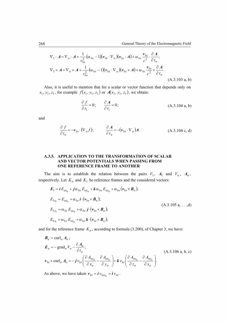
General Theory of the Electromagnetic Field
268
( )( )( )
( )( )( ) .11
;11
o2o1
o1o1oo1o12o1
o1
o2o1
o1o1oo1o12o1
o1
tcv
tcv
∂∂
×α+×∇⋅−α+×∇=×∇
∂∂
⋅α+⋅∇⋅−α+⋅∇=⋅∇
AvAvvAA
AvAvvAA
(A.3.103 a, b)
Also, it is useful to mention that for a scalar or vector function that depends only on 111 ,, zyx , for example ( )111 ,, zyxf or ( )111 ,, zyxA , we obtain:
;0;011=
∂∂
=∂∂
ttf A (A.3.104 a, b)
and
( ) ( ) .; oo1o
oo1o
AvAv ∇⋅−=∂∂
∇⋅−=∂∂
tf
tf (A.3.104 c, d)
A.3.5. APPLICATION TO THE TRANSFORMATION OF SCALAR AND VECTOR POTENTIALS WHEN PASSING FROM ONE REFERENCE FRAME TO ANOTHER
The aim is to establish the relation between the pairs 1V , 1A and oV , oA , respectively. Let oK and 1K be reference frames and the considered vectors:
( )
( )
( )
( );
;
;
;
oo1o1oo11
oo1o1oo11
oo1o1o1
oo1o1oo1oo1o1
o1
o1
o1
ooo
Bvk
Bvj
Bvi
BvkjiE
×⋅α+α=
×⋅α+α=
×⋅α+=
×α+α+α+=
zz
yy
xx
zyx
EE
EE
EE
EEE
(A.3.105 a, . . .,d)
and for the reference frame oK , according to formula (3.200), of Chapter 3, we have:
.curl
;grad
;curl
o
o
o
oo1
o
o
o
oo1ooo1
o
oooo
ooo
oooo⎟⎟⎠
⎞⎜⎜⎝
⎛
∂
∂−
∂
∂+⎟⎟
⎠
⎞⎜⎜⎝
⎛
∂
∂−
∂
∂−=×
∂∂
−−=
=
xA
zA
vy
Ax
Av
tV
zxxy kjAv
AE
AB
(A.3.106 a, b, c)
As above, we have taken o1o1o1 ovv x iiv == .
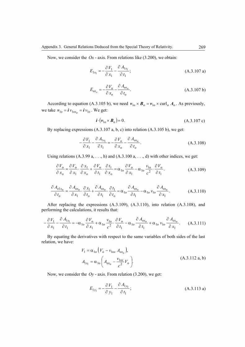
Appendix 3. General Relations Deduced from the Special Theory of Relativity.
269
Now, we consider the Ox - axis. From relations like (3.200), we obtain:
;1
1
1
11
11 t
AxV
E xx ∂
∂−
∂∂
−= (A.3.107 a)
.o
o
o
oo
oo t
AxVE x
x ∂
∂−
∂∂
−= (A.3.107 b)
According to equation (A.3.105 b), we need ooo1oo1 curl AvBv ×=× . As previously, we take o1o1o1 o
vv x iiv == . We get:
( ) .0oo1 =×⋅ Bvi (A.3.107 c)
By replacing expressions (A.3.107 a, b, c) into relation (A.3.105 b), we get:
.o
o
o
o
1
1
1
1 o1
t
A
xV
tA
xV xx
∂
∂−
∂∂
−=∂
∂−
∂∂
− (A.3.108)
Using relations (A.3.99 a, . . ., h) and (A.3.100 a, . . ., d) with other indices, we get:
.1
o2o1
o11
oo1
o
1
1
o
o
1
1
o
o
o
tV
cv
xV
xt
tV
xx
xV
xV
∂∂⋅α−
∂∂
α=∂∂
⋅∂∂
+∂∂
⋅∂∂
=∂∂
(A.3.109)
.1
oo1o1
1
oo1
o
1
1
o
o
1
1
o
o
o1 ooooo
xA
vt
Att
tA
tx
xA
tA xxxxx
∂
∂α−
∂
∂α=
∂∂⋅
∂
∂+
∂∂⋅
∂
∂=
∂
∂ (A.3.110)
After replacing the expressions (A.3.109), (A.3.110), into relation (A.3.108), and performing the calculations, it results that:
.1
oo1o1
1
oo1
1
o2o1
o11
oo1
1
1
1
1 oo1
x
Av
t
A
tV
cv
xV
tA
xV xxx
∂
∂α+
∂
∂α−
∂∂⋅α+
∂∂
α−=∂
∂−
∂∂
− (A.3.111)
By equating the derivatives with respect to the same variables of both sides of the last relation, we have:
( ).
,
o2o1
oo11
oo1oo11
o1
o
⎟⎠
⎞⎜⎝
⎛ −α=
−α=
Vc
vAA
AvVV
xxx
xx
(A.3.112 a, b)
Now, we consider the Oy - axis. From relation (3.200), we get:
;1
1
1
11
11 t
AyV
E yy ∂
∂−
∂∂
−= (A.3.113 a)
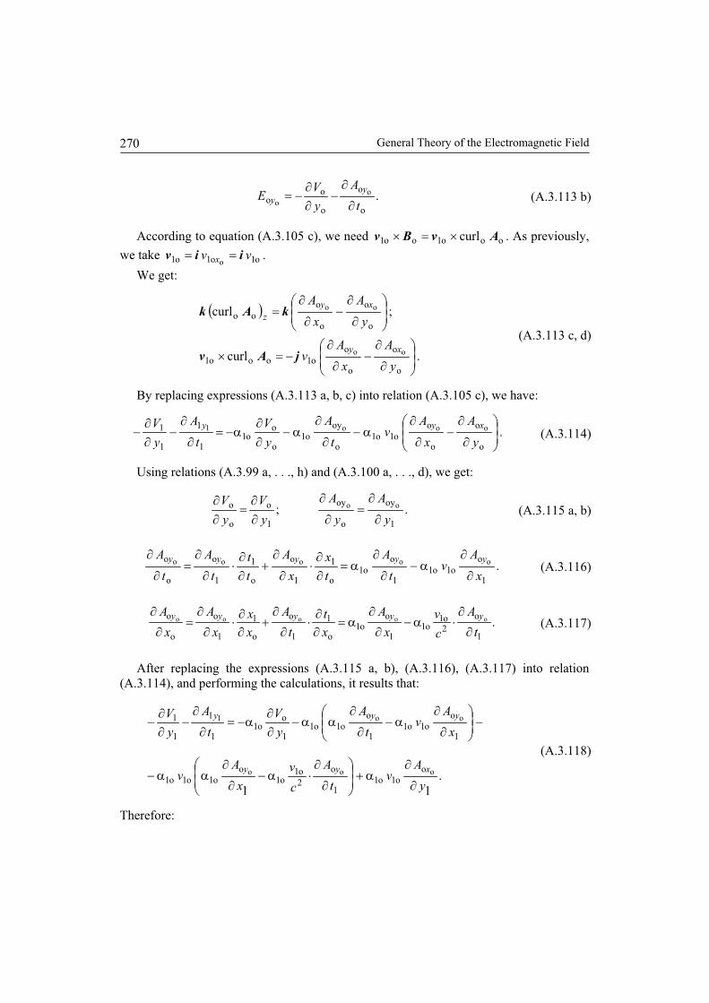
General Theory of the Electromagnetic Field270
.o
o
o
oo
oo t
A
y
VE
y
y (A.3.113 b)
According to equation (A.3.105 c), we need ooo1oo1 curl AvBv . As previously,
we take o1o1o1 ovv x iiv .
We get:
.curl
;curl
o
o
o
oo1ooo1
o
o
o
ooo
oo
oo
y
A
x
Av
y
A
x
A
xy
xy
z
jAv
kAk
(A.3.113 c, d)
By replacing expressions (A.3.113 a, b, c) into relation (A.3.105 c), we have:
.o
o
o
oo1o1
o
oyo1
o
oo1
1
1
1
1 ooo1
y
A
x
Av
t
A
y
V
t
A
y
V xyy(A.3.114)
Using relations (A.3.99 a, . . ., h) and (A.3.100 a, . . ., d), we get:
.;1
oy
o
oy
1
o
o
o oo
y
A
y
A
y
V
y
V(A.3.115 a, b)
.1
oo1o1
1
oo1
o
1
1
o
o
1
1
o
o
o ooooo
x
Av
t
A
t
x
x
A
t
t
t
A
t
A yyyyy(A.3.116)
.1
o2o1
o11
oo1
o
1
1
o
o
1
1
o
o
o ooooo
t
A
c
v
x
A
x
t
t
A
x
x
x
A
x
A yyyyy(A.3.117)
After replacing the expressions (A.3.115 a, b), (A.3.116), (A.3.117) into relation(A.3.114), and performing the calculations, it results that:
.11
ooo
oo1
oo1o1
1
o
2o1
o1o
o1o1o1
1
oo1o1
1
oo1o1
1
oo1
1
1
1
1
y
Av
t
A
c
v
x
Av
x
Av
t
A
y
V
t
A
y
V
xyy
yyy
(A.3.118)
Therefore:
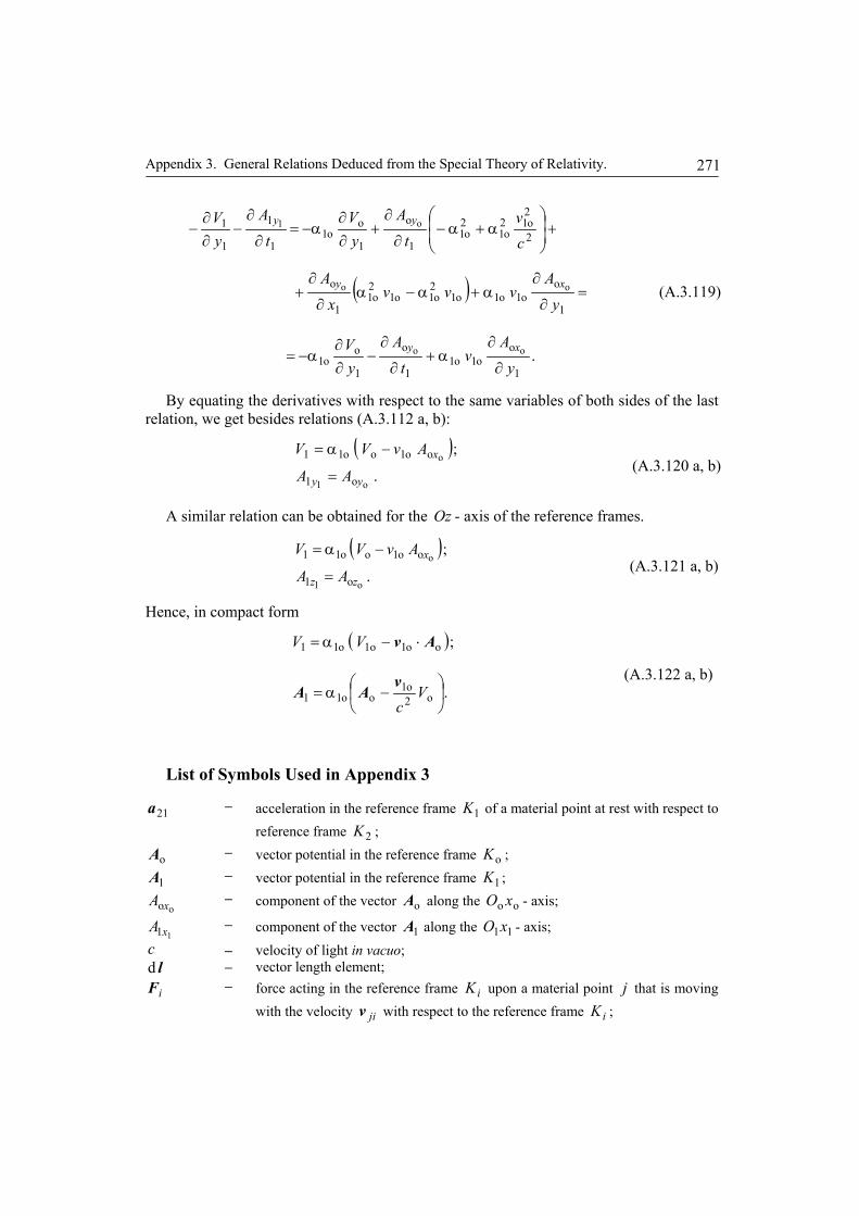
Appendix 3. General Relations Deduced from the Special Theory of Relativity. 271
( )
.1
oo1o1
1
o
1
oo1
1
oo1o1o1
2o1o1
2o1
1
o
2
2o12
o12o1
1
o
1
oo1
1
1
1
1
oo
oo
o1
y
Av
t
A
yV
y
Avvv
x
A
cv
t
A
yV
t
A
yV
xy
xy
yy
∂
∂α+
∂
∂−
∂∂
α−=
=∂
∂α+α−α
∂
∂+
+⎟⎟⎠
⎞⎜⎜⎝
⎛α+α−
∂
∂+
∂∂
α−=∂
∂−
∂∂
−
(A.3.119)
By equating the derivatives with respect to the same variables of both sides of the lastrelation, we get besides relations (A.3.112 a, b):
( ).
;
o1
o
o1
oo1oo11
yy
x
AA
AvVV
=
−α=(A.3.120 a, b)
A similar relation can be obtained for the Oz - axis of the reference frames.
( ).
;
o1
o
o1
oo1oo11
zz
x
AA
AvVV
=
−α=(A.3.121 a, b)
Hence, in compact form
( )
.
;
o2o1
oo11
oo11oo11
⎟⎠
⎞⎜⎝
⎛−α=
⋅−α=
Vc
VV
vAA
Av
(A.3.122 a, b)
List of Symbols Used in Appendix 3
21a – acceleration in the reference frame 1K of a material point at rest with respect toreference frame 2K ;
oA – vector potential in the reference frame oK ;
1A – vector potential in the reference frame 1K ;
ooxA – component of the vector oA along the oo xO - axis;
11xA – component of the vector 1A along the 11xO - axis;c – velocity of light in vacuo;
ld – vector length element;
iF – force acting in the reference frame iK upon a material point j that is movingwith the velocity jiv with respect to the reference frame iK ;
General Theory of the Electromagnetic Field272
irF – rest component of the force iF corresponding to the case in which the material
point would be at rest with respect to the reference frame iK ;
ivF – motion component of the force iF arising in the case in which the material
point is moving with the velocity jiv with respect to the reference frame iK ;
iK – symbol of an inertial reference frame, where the space co-ordinates have beendenoted ix , iy , iz , and the time it ;
m – relativistic mass of the material point in motion with the velocity u , withrespect to any inertial reference frame K ;
0m – rest mass of a material point, at rest with respect to any reference frame K ,expressed in the same reference frame; if no other mention is made, then bymass is understood the rest mass;
q – electric charge of a point-like body;
or – position vector of a point in the reference frame oK , with its origin at the
origin of the same reference frame;
1r – position vector of a point in the reference frame 1K , with its origin at the
origin of the same reference frame;
ot – time in the reference frame oK ;
1t – time in the reference frame 1K ;u – velocity of a material point in any reference frame K ;v – velocity of any reference frame relative to the reference frame K ;
o1v – velocity of the reference frame 1K relatively to the reference frame oK ;
o2v – velocity of the reference frame 2K or of a material point denoted by 2,
relatively to the reference frame oK ;
jiv – velocity of a point denoted by j or of any reference frame jK relatively to the
reference frame iK ;
oV – scalar potential in the reference frame oK , p. 268; volume, p. 248;
1V – scalar potential in the reference frame 1K , p. 268; volume, p. 248, 261;
ooo ,, zyx – co-ordinates in the system of co-ordinates of oK ;
111 ,, zyx – co-ordinates in the system of co-ordinates of 1K ;
;1
1
1
122ijij
ij
c
ijij
v;
iS – vector surface element in the reference frame iK ;
vi – volume density of the electric charge in the reference frame iK .
The symbols with one index refer to a certain reference frame, for instance 1K .
The symbols with two indices refer to quantities concerning two systems, for instance o2v
represents the velocity of the reference frame 2K relatively to the reference frame oK .

APPENDIX 4
DEDUCING THE GENERAL RELATIONS OF THE SPECIAL THEORY OF RELATIVITY
In this Appendix, we shall present a deduction of certain basic relations of the Theory of Special Relativity concerning Mechanics, which we have used in Appendix 3. The deductions differ from the usual ones and are closed to the concerned applications.
A.4.1. DERIVING THE CO-ORDINATE TRANSFORMATION RELATIONS FOR PASSING FROM ONE SYSTEM OF CO-ORDINATES TO ANOTHER ONE
We shall consider two systems of Cartesian co-ordinates, denoted K and 'K . The axes of co-ordinates of the two systems are parallel to each other. The time and space co-ordinates of K will be t, x, y, z, and c will represent the velocity of light in vacuo, and will be assumed to be constant. The system K will be considered as fixed and the system
'K will be considered in translation motion, with the constant velocity v, along the Ox - axis of K. At the first moment, i.e., at 0=t , we shall suppose that the origins O and O′ of the two systems of co-ordinates coincide.
The fundamental relation assumed in the Special and General Theory of Relativity is represented by one invariant, namely the constant value of the space-time interval:
[ ] ;;;;;3,0;ddd 32102 zxyxxxctxixxgs jiij ====∈∀= (A.4.1 a-e)
where ijg represents the general term of the fundamental tensor, regardless of the system of reference. The relation (A.4.1) is called the fundamental time-space relation or fundamental form of the metric relation of the considered space.
In the case of a Galilean system of co-ordinates:
( ) [ ] ;;;;3,1,ddd 3212222 zxyxxxixtcs i ===∈∀−= (A.4.2 a-d)
and then, the corresponding quadratic form (A.4.1) becomes (A.4.2) and is called normal or quasi-Euclidean form.
Since we have considered the motion only along the Ox - axis, we shall take into consideration, apart from the time co-ordinate, only the x co-ordinate involved in the motion, whereas the co-ordinates y and z are not affected. The co-ordinates of the system
'K will be denoted like those of K, but with the sign prime.

General Theory of the Electromagnetic Field
274
We shall look for the relations between the co-ordinates in the two systems of co-ordinates of above. So far, in the previous published works, these relations have been usually obtained through relatively complicated geometrical deductions, which we shall avoid. For this purpose we shall express the involved co-ordinates of the system K versus those of 'K , namely x and t.
A linear dependence will be assumed, as follows:
.,
xqtpttbxax′+′=
′+′= (A.4.3 a, b)
From the condition of the constant value of the space-time interval (A.4.2 a), we get the following relation:
( )( ) ( ) ( )( ) 0ddd2d 222222222 =′−−′′−+′− xqcatxabpqctbpc . (A.4.4)
By identifying the coefficients, there follows:
.
,1
,
2
222
2222
abpqc
aqc
cbpc
=
−=−
=−
(A.4.5 a, b, c)
By replacing p and q from (A.4.5 a) and (A.4.5 b) into (A.4.5 c), we get:
( )( )
.;
;1
;11
2
2
224
2222
cbqap
acb
bac
cbac
==
−=
=+−
(A.4.6 a-d)
For the square root, we have taken the sign plus and we shall examine further the case which corresponds to the chosen sign.
We shall consider any point fixed in the system K ′ , for instance the origin O′ , with ,0=′x its velocity in the system K will be v along the direction of the increasing values
of the co-ordinate 'x . Considering relations (A.4.3 a, b), and replacing ,0=′x there follows:
.;;
;;1
1;dd
2
2
cvqpvb
cvav
pb
tx
α=α=α=
=ββ−
==α==
(A.4.7 a-f)
Appendix 4. Deducing the General Relations of the Special Theory of Relativity.
275
Using relations (A.4.3) and (A.4.7), and including also the relations containing the co-ordinates unaffected by the co-ordinate transformation, there follows:
( )
.;
;
;
2
zzyy
xcvtt
tvxx
′=′=
⎟⎠
⎞⎜⎝
⎛ ′+′α=
′+′α=
. (A.4.8 a-d)
For the inverse transformation, by solving the system given by (A.4.8), we obtain:
( )
;;
;
;
2
zzyy
xcvtt
vtxx
=′=′
⎟⎠
⎞⎜⎝
⎛ −α=′
−α=′
(A.4.9 a-c)
where we can remark the change of sign. From these sets of relations, it results directly that simultaneous events in frame K ′ are not simultaneous in frame K, and conversely.
Also, from relation (A.4.8 b), it follows that for a clock located at any fixed point of the frame K ′ , one obtains tt ′Δα=Δ , hence tt ′Δ>Δ , so that we deal with a dilation of time.
In addition, from relation (A.4.9 a), it follows that, for a ruler placed in K ′ along the xO ′′ - axis, at any given time t, one obtains xx Δα=′Δ , hence xx Δ>′Δ , so that we now
deal with a contraction of length.
A.4.2. DERIVING THE EXPRESSION OF THE ADDITION OF VELOCITIES
Further on, in order to give more suggestive explanations, we shall denote the reference frames K and K ′ , by oK and 1K , respectively, where the original frame K, assumed as immobile, is indicated by the upright subscript o, whereas the moving frame is indicated by the subscript 1. We shall similarly denote the quantities belonging to these systems. The constant velocity of 1K relatively to oK will be denoted xv o1o1 iv = .
Let us consider a point P, moving with the velocity 21v relatively to the reference frame 1K . At any time, if 1x is the co-ordinate of a point in 1K , the corresponding co-ordinates in oK are consequently:
( )
.
;;1
1;
12o1
1o10
o1o12
o1o11o11o1o
⎟⎠
⎞⎜⎝
⎛+α=
=ββ−
=α+α=
xc
vtt
cv
tvxx
x
xx
(A.4.10 a-d)

General Theory of the Electromagnetic Field
276
The velocity xv o2 of point P in oK will be obtained by using relations (A.4.8 a, b) with the modified symbols as explained above:
( )[ ] ( )[ ]
.1
,
dd
1
dd
dd
dd
d
ddd
dd
221o1
o1212ox
1
12o1
o11
1
12o1
1
1o11
12o1
1o1
1o11o11o11o1
oo
oo2
cvvvv
v
tx
cv
vtx
xc
vt
tvx
xc
vt
tvxtvx
ttx
v
xx
xx
x
x
x
x
x
xxx
+
+=
⋅+
+=
+
+=
=
⎥⎦
⎤⎢⎣
⎡⎟⎠
⎞⎜⎝
⎛+α
+α=+α==
(A.4.11 a, b)
Further on, we shall take into account that no difference occurs between oy and oz relatively to 1y and 1z .
As previously shown for xv o2 , there follows:
.1
;1
;
dd
1
dd
d
ddd
221o1
o1
21o2
221o1
o1
21o2
1
12o1
o1
1
1
12o1
1o1
1
o
oo2
⎟⎠
⎞⎜⎝
⎛+α
=⎟⎠
⎞⎜⎝
⎛+α
=
⎟⎟⎠
⎞⎜⎜⎝
⎛⋅+α
=
⎥⎦
⎤⎢⎣
⎡⎟⎠
⎞⎜⎝
⎛+α
==
cvv
vv
cvv
vv
tx
cv
ty
xc
vt
yty
v
xx
zz
xx
yy
xxy
(A.4.12 a-c)
Calculating the derivatives with respect to time, like previously, we shall get the expressions of the accelerations.
A.4.3. RELATIONSHIP BETWEEN MASS AND VELOCITY
According to one of the postulates of the Theory of Special Relativity (Chapter 2, p. 99), the mechanical momentum (quantity of motion) along any direction perpendicular to the direction of motion is kept (conserved) when passing from an inertial reference frame oK to another 1K . Therefore, for any material point 2, with the mass om , we can write the following relations:
yxx
yyy vm
cvv
vmvmvm 211
221o1
o1
21o211o2o
1; =
⎟⎠⎞
⎜⎝⎛ +α
= , (A.4.13)
Appendix 4. Deducing the General Relations of the Special Theory of Relativity.
277
where the factor yv 12 may be simplified. We shall, now, consider the material point at
rest in the reference frame 1K , and in this case, 021 =xv , and the mass of the material point in a reference frame in which the point is at rest, called proper mass, will be denoted by 0m (the subscript is zero not o, as for other symbols, o0 mm ≠ ). By replacing the value of the velocity 021 =xv , we get:
.
1
10
2
2o1
1 m
cv
mm
−
== (A.4.14)
A similar relation may be written for any system of reference.
A.4.4. RELATIONS BETWEEN THE FORCES OF TWO SYSTEMS OF REFERENCE
The components of the force will be calculated by the derivatives with respect to time of the components of the momentum (quantity of motion).
A.4.4.1. Expression of the Components along the Ox - axis
The expression of the force acting on a material point P, along the Ox - axis, will be:
⎥⎥⎥
⎦
⎤
⎢⎢⎢
⎣
⎡
⎟⎟⎠
⎞⎜⎜⎝
⎛−=
−
xx vcv
mt
F o221
2
2o2
0o
o 1dd , (A.4.15)
where 0m (the index of m is zero not o) denotes, like above, the proper mass of the point, considered as a material point, in a reference frame in which the point is at rest. By using relations (A.4.11) and (A.4.12), we shall obtain:
.1
111
221o1
o1
21
2
221
21
2
2o2
⎟⎠
⎞⎜⎝
⎛+α
⎟⎟⎠
⎞⎜⎜⎝
⎛−=⎟
⎟⎠
⎞⎜⎜⎝
⎛−
cvvc
vcv
xx (A.4.16)
For obtaining relation (A.4.16), have had to replace (A.4.11 b), (A.4.12 b), (A.4.12 c) in the left-hand side of relation (A.4.16), hence in (A.4.16 a), below:
.; 221
221
221
221
22o
22o
22o
22o zyxzyx vvvvvvvv ++=++= (A.4.16 a)
General Theory of the Electromagnetic Field
278
By performing the calculations, we have obtained as an intermediate result the following expression:
,c
1
21o12
221
2o1
221
2221
2o1
221
2221
22o1
22o1
2o1
4
2
2o2
xx
zxzyvxyxxxx
vvcvvvcvvvcvcvcvv
cv
+
+−+−−−+=
=−
(A.4.16 b)
and grouping the terms of the numerator in formula (A.4.16 b), we obtain the right-hand side of relation (A.4.16). The component of the force along the Ox - axis in the considered systems of reference
oK , results as follows:
.1dd1
dd
dd1
1
1d1ddd
1
dd
;v1111
;dd1
dd
o121
2
221
01
2121
2
221
01
1
12o1
o121
2
221
02121
2
221
0
12o1
1
10
o1
oo
221o1
o121221o1
1021
2
221
0o221
2
2o2
0
oo2
21
2
2o2
0o
o
⎪⎭
⎪⎬
⎫
⎪⎩
⎪⎨
⎧
⎥⎥⎥
⎦
⎤
⎢⎢⎢
⎣
⎡
⎟⎟⎠
⎞⎜⎜⎝
⎛−+
⎥⎥⎥
⎦
⎤
⎢⎢⎢
⎣
⎡
⎟⎟⎠
⎞⎜⎜⎝
⎛−
⋅+=
=⎪⎭
⎪⎬
⎫
⎪⎩
⎪⎨
⎧
⎥⎥⎥
⎦
⎤
⎢⎢⎢
⎣
⎡
⎟⎟⎠
⎞⎜⎜⎝
⎛−+
⎥⎥⎥
⎦
⎤
⎢⎢⎢
⎣
⎡
⎟⎟⎠
⎞⎜⎜⎝
⎛−
+
α⋅
α=
==
+
+⎟⎠⎞
⎜⎝⎛ +α⎟
⎟⎠
⎞⎜⎜⎝
⎛−=⎟
⎟⎠
⎞⎜⎜⎝
⎛−=
=⎥⎥⎥
⎦
⎤
⎢⎢⎢
⎣
⎡
⎟⎟⎠
⎞⎜⎜⎝
⎛−=
−−
−−
−−
−
xxx
xxx
x
xx
xxxxx
xx
vcvm
tv
cvm
ttx
cv
vcvmv
cvm
xc
vt
tSF
cv
vvc
vcvmv
cvmS
tSv
cvm
tF
v
(A.4.17a-c)
Therefore:

Appendix 4. Deducing the General Relations of the Special Theory of Relativity.
279
( )
.1dd
;1dd;
1
1
;1
11dd1
dd
o121
2
221
01
2121
2
221
01
11
221o1
o
221o1
o121
2
212
01
2121
2
212
01
o
⎥⎥⎥
⎦
⎤
⎢⎢⎢
⎣
⎡
⎟⎟⎠
⎞⎜⎜⎝
⎛−=
⎥⎥⎥
⎦
⎤
⎢⎢⎢
⎣
⎡
⎟⎟⎠
⎞⎜⎜⎝
⎛−=+
+=
+⎪⎭
⎪⎬
⎫
⎪⎩
⎪⎨
⎧
⎥⎥⎥
⎦
⎤
⎢⎢⎢
⎣
⎡
⎟⎟⎠
⎞⎜⎜⎝
⎛−+
⎥⎥⎥
⎦
⎤
⎢⎢⎢
⎣
⎡
⎟⎟⎠
⎞⎜⎜⎝
⎛−=
−
−
−−
x
xxxxx
x
xxxxx
vcvm
tR
vcvm
tFRF
cvvF
cvvv
cvm
tv
cvm
tF
(A.4.18a-c)
There remains to calculate the term R. We can write:
( )
( ),11
11
1dd
212123
2
221
02o1
21212121212123
2
221
02o1
o121
2
221
01
vv &
&&&
⋅⎟⎟⎠
⎞⎜⎜⎝
⎛−=
=++⎟⎟⎠
⎞⎜⎜⎝
⎛−=
=⎥⎥⎥
⎦
⎤
⎢⎢⎢
⎣
⎡
⎟⎟⎠
⎞⎜⎜⎝
⎛−=
−
−
−
cvm
cv
vvvvvvcvm
cv
vcvm
tR
x
zzyyxxx
x
(A.4.19)
where, for simplicity, we have denoted 1
2121 d
dtv
v =& .
The expression of R is, to some extent, similar to that of xF1 but includes a scalar product. Therefore, we shall express xF1 using also a vector form:
.11
1
1dd
2121
2
221
021
2
221
2
221
21
2
221
0
2121
2
221
01
1
vv
vF
&&
−−
−
⎟⎟⎠
⎞⎜⎜⎝
⎛−+
⎟⎟⎟⎟⎟
⎠
⎞
⎜⎜⎜⎜⎜
⎝
⎛
−⎟⎟⎠
⎞⎜⎜⎝
⎛−=
=⎥⎥⎥
⎦
⎤
⎢⎢⎢
⎣
⎡
⎟⎟⎠
⎞⎜⎜⎝
⎛−=
cvm
cv
cv
cvm
cvm
t
(A.4.20)
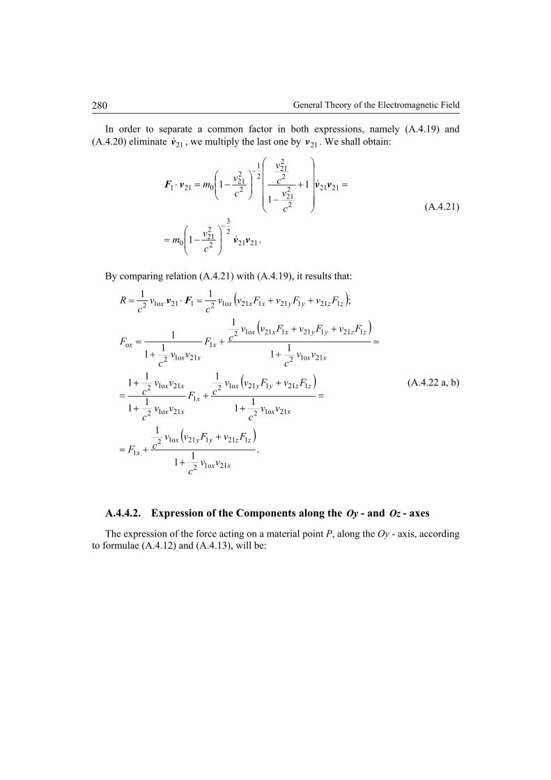
General Theory of the Electromagnetic Field
280
In order to separate a common factor in both expressions, namely (A.4.19) and (A.4.20) eliminate 21v& , we multiply the last one by 21v . We shall obtain:
.1
11
1
212123
2
221
0
2121
2
221
2
221
21
2
221
0211
vv
vvvF
&
&
−
−
⎟⎟⎠
⎞⎜⎜⎝
⎛−=
=
⎟⎟⎟⎟⎟
⎠
⎞
⎜⎜⎜⎜⎜
⎝
⎛
+−
⎟⎟⎠
⎞⎜⎜⎝
⎛−=⋅
cvm
cv
cv
cvm
(A.4.21)
By comparing relation (A.4.21) with (A.4.19), it results that:
( )
( )
( )
( ).11
1
11
1
11
11
11
1
11
1
;11
211o2
121121o121
21o12
121121o121
21o12
21o12
21o12
121121121o121
21o12
o
121121121o12121o12
xx
zzyyx
x
xx
zzyyx
x
xx
xx
xx
zzyyxxx
x
xx
x
zzyyxxxx
vvc
FvFvvcF
vvc
FvFvvcF
vvc
vvc
vvc
FvFvFvvcF
vvc
F
FvFvFvvc
vc
R
+
++=
=+
++
+
+=
=+
+++
+=
++=⋅= Fv
(A.4.22 a, b)
A.4.4.2. Expression of the Components along the Oy - and Oz - axes
The expression of the force acting on a material point P, along the Oy - axis, according to formulae (A.4.12) and (A.4.13), will be:

Appendix 4. Deducing the General Relations of the Special Theory of Relativity.
281
.1
111dd
1
11
;
dd1
dd
1
dd
d1
;1v1
v11
1
;dd
d1dd
1
221o1o1
2121
2
221
01
221o1o1
o
1
12o1
1
o112
o11
o1o
2121
2
221
0
221o1
o1
212
21o1o1
21
2
221
0
oy221
2
2o2
0
12o1
1o1
oy221
2
2o2
0o
o
yxx
yxx
y
xxy
yxx
yxx
xy
F
cvvv
cvm
tcvvF
tx
cv
tS
xc
vt
SF
vcvm
cv
v
cv
cvm
vcvmS
xc
vt
Svcvm
tF
⋅+
⋅α
=⎥⎥⎥
⎦
⎤
⎢⎢⎢
⎣
⎡
⎟⎟⎠
⎞⎜⎜⎝
⎛−⋅
+⋅
α=
⋅+⋅
α=
+⋅
α=
⎟⎟⎠
⎞⎜⎜⎝
⎛−=
⎟⎠⎞
⎜⎝⎛ +α
⎟⎠⎞
⎜⎝⎛ +α⎟
⎟⎠
⎞⎜⎜⎝
⎛−=
=⎟⎟⎠
⎞⎜⎜⎝
⎛−=
⎟⎠⎞
⎜⎝⎛ +α
=⎥⎥⎥
⎦
⎤
⎢⎢⎢
⎣
⎡
⎟⎟⎠
⎞⎜⎜⎝
⎛−=
−
−−
−
−
(A.4.23a-c)
Similarly, we can obtain the expression of zFo .
A.4.4.3. Expressions of All Components
For obtaining compact expressions in view of many applications, we shall use the symbols and expressions below:
ccc21
21o2
o2o1
o1 ;; vβvβvβ === . (A.4.24 a-c)
With these symbols, and assuming that xvi o1o1 =β , relations (A.4.22) and (A.4.23) becomes:
.ββ1
11;ββ1
11
;11
1ox121o1
oz1ox121o1
o
121o1
21o11
21o1
21o11o
zx
yx
y
zxx
zxy
xx
yxxx
FFFF
FFFF
⋅+⋅
α=
⋅+⋅
α=
β⋅β+ββ
+β⋅β+
ββ+=
(A.4.25 a-c)
Combining the formulae (A.4.24) and (A.4.25), we can write all relations in the following vector form:

General Theory of the Electromagnetic Field
282
( ) ( )( ) .
11
11
11
;1
11;1
11
;1c1
1
;;;
o121
11o2121o12
o1
o1
o121o1
o11
o121o1
o121o1o
121o1o1
oz121o1o1
o
21o1
121o11
21o1o
2121
o2o2
o1o1
ββFvvFvv
ββF
ββββF
ββββ
ββFβ
ββ
vβvβvβ
⋅+××
⋅+⋅⋅⋅+α
−α+
⋅+α⋅α+
=
⋅+⋅
α=
⋅+⋅
α=
⋅+⋅
⋅+⋅+
=
===
cv
FFFF
vFF
ccc
zyy
xxx
(A.4.26a-g)

APPENDIX 5
THE EQUATIONS OF THE ELECTROMAGNETIC FIELD IN THE GENERAL THEORY OF RELATIVITY
In this Appendix, we shall present the equations of the electromagnetic field in the Special and General Theory of Relativity. We shall begin with the covariant forms of the equations, so that the passage from the Special to the General Theory of Relativity could be performed without difficulties. The bibliographic mentions [1]-[12], specific for this Appendix, are at the end of this Appendix. Also, a list of symbols is given at the end of this Appendix. In the known literature various methods are used [1]-[11]. We shall have in view the works [8], [9], which present certain advantages for the purpose of this Appendix.
A.5.1. THE FOUR POTENTIAL TENSOR OF RANK 1 AND THE TENSORS OF RANK 2
From the formulae of the general theory of the electromagnetic field (Chapter 3, p. 129, 134, 142, 150, 182), in the usual vector form, we have:
.;;curl
;grad;curl;curl
000 MHBPEDDJH
AEABBE
µ+µ=+ε=∂∂
+=
∂∂
−−==∂∂
−=
t
tV
t (A.5.1 a, …, f)
We shall rewrite the equations (A.5.1) considering the general case of non-linear media:
( )
.curlgraddivgrad
;curlgradcurlcurlcurl
;curlcurl
02
2
0002
0000
0000000
⎟⎟⎠
⎞⎜⎜⎝
⎛+
∂∂
µ+⎟⎟⎠
⎞⎜⎜⎝
⎛
∂∂
+∂∂
µε−µ=∇−
⎟⎟⎠
⎞⎜⎜⎝
⎛+
∂∂
µ+⎟⎟⎠
⎞⎜⎜⎝
⎛∂∂
−−∂∂
µε+µ==
µ+∂∂
µ+∂∂
µε+µ=µ+µ
MPAJAA
MPAJAB
MPEJMH
tttV
ttV
t
tt
(A.5.2 a-c)
Rearranging the terms of (A.5.2 c), we get:

General Theory of the Electromagnetic Field
284
.divgradcurl 0002
2
002
⎟⎟⎠
⎞⎜⎜⎝
⎛∂∂
µε++⎟⎟⎠
⎞⎜⎜⎝
⎛+
∂∂
+µ−=∂
∂µε−∇
tV
ttAMPJAA (A.5.3)
Since only the curl of vector A is imposed, the divergence can be chosen by using the L. V. Lorenz (not to be confused with H. A. Lorentz) gauge condition:
0div 00 =∂∂
µε+tVA . (A.5.4)
The last relation may be written in the form:
[ ]00
200
1;;3,1,01µε
==∈=∂
∂⋅+
∂
∂ctcxi
xV
cxA
ii . (A.5.4 a, b, c)
The components along any axis of a Cartesian system of co-ordinates will be:
[ ]3,1,,;,; ∈∀≠∀∂
∂−
∂
∂=
∂∂
−∂
∂−= kjikj
x
A
xA
BtA
xVE k
jjk
ii
ii . (A.5.5 a, b)
The relations (A.5.1 a, b) may be written using a set of four quantities iA as follows:
[ ] .;3,1,,,, 00 VAkji
x
A
xA
BtA
xA
E kj
jk
ii
ii −=∈∀∂
∂−
∂
∂=
∂∂
−∂
∂= (A.5.6 a, b, c)
A.5.2. ESTABLISHING THE NATURE OF THE TENSORS
A tensor is in fact a geometrical object, the vector being a particular case. By the nature of a tensor is meant its character, namely whether when passing from one system of reference to another one, the tensor will be transformed as a contravariant or as a covariant one.
If the geometrical object, which will be defined as a tensor, is considered separately, with no relation with other tensors, each of the two variants may be chosen. If it is considered in relation with other tensors, its nature being established, the situation is different. For example, it is necessary to mention that if the product of two tensors yields a result of a certain nature, say a scalar (tensor of rank 0), the product should give the same result in any other system of reference.
If the character of one tensor is established and we have to choose the character of a geometrical object that will constitute the other tensor, one can use the known procedures: the tensor quotient law [5, p. 167] or the theorem of tensor classification [10, p. 376]. We shall extend the last one, using integral operators, in order to facilitate the procedure.

Appendix 5. The Equations of the Electromagnetic Field in the General Theory of Relativity.
285
In order to fix the ideas, we shall establish the nature of the set of four quantities iA that may be functions of co-ordinates. Several explanations have been given in literature on this subject, some of them referring to formula (A.5.4), but without a precise conclusion [12].
However, we consider that this analysis may be carried out as follows. We shall refer to Section 3.10 where the transition from the system of reference K to the system of reference K ′ , both being inertial systems, is examined. We shall take into consideration that 0AV −= in (3.115) and (3.116 a), of Chapter 3, as in (A.5.6 c). Rewriting those relations using the symbols above, and replacing iA by iAc for 0≠i , there follows:
;;;; 3322101100 AAAAAAcvAA
cvAA =′=′⎟
⎠⎞
⎜⎝⎛ +α=′⎟
⎠⎞
⎜⎝⎛ +α=′ (A.5.7 a, …, d)
and:
.;;; 3322101100 xxxxxxcvxx
cvxx =′=′⎟
⎠⎞
⎜⎝⎛ +−α=′⎟
⎠⎞
⎜⎝⎛ −α=′ (A.5.7 e, …, h)
By comparing the two systems of relations, it follows that the set 3210 ,,, AAAA and
the set 3210 ,,, xxxx change in different manners. Therefore, the latter set being a contravariant four-vector, the former will be a covariant four-vector. Then, we can renounce the replacement. According to Linear Algebra relationships, if the set
3210 ,,, AAAA is a covariant tensor of rank 1, each set obtained from the previous one by multiplying each element (component) by any constant factor, will also be a covariant four-vector, i.e., hence a tensor of rank 1. Therefore the set [ ]3,0, ∈∀ iAi , is a covariant four-vector.
In general, in any multidimensional continuum (space), in the present case, a four-dimensional one, any set of four quantities, that is a geometrical object with four components (elements), which can be functions of co-ordinates, may constitute a tensor of rank 1, provided the transformation formulae when passing from a reference frame to another, are like the transformation formulae of the co-ordinates, or opposite. In the former case the tensor will be called contravariant tensor, and in the latter one, the tensor will be called covariant tensor.
From the mathematical point of view, we can choose any of those transformation formulae. It should be added that regardless of the chosen formulae, the length of the tensor will be the same, only the components will differ. From the physical point of view, it is useful to choose a transformation, which is in good agreement with the physical conditions, and requires the smallest volume of computations. Moreover, it is necessary that the nature of tensors entering an equation should be the same, otherwise the equation being not valid.
Having these possibilities in choosing the nature of the geometrical object above, we shall consider it as a covariant tensor of rank 1, which is a covariant four-vector.
We shall make a first verification in order to examine the previous choice. Let us consider relation (A.5.1 b), and calculate the flux of vector B through any simply
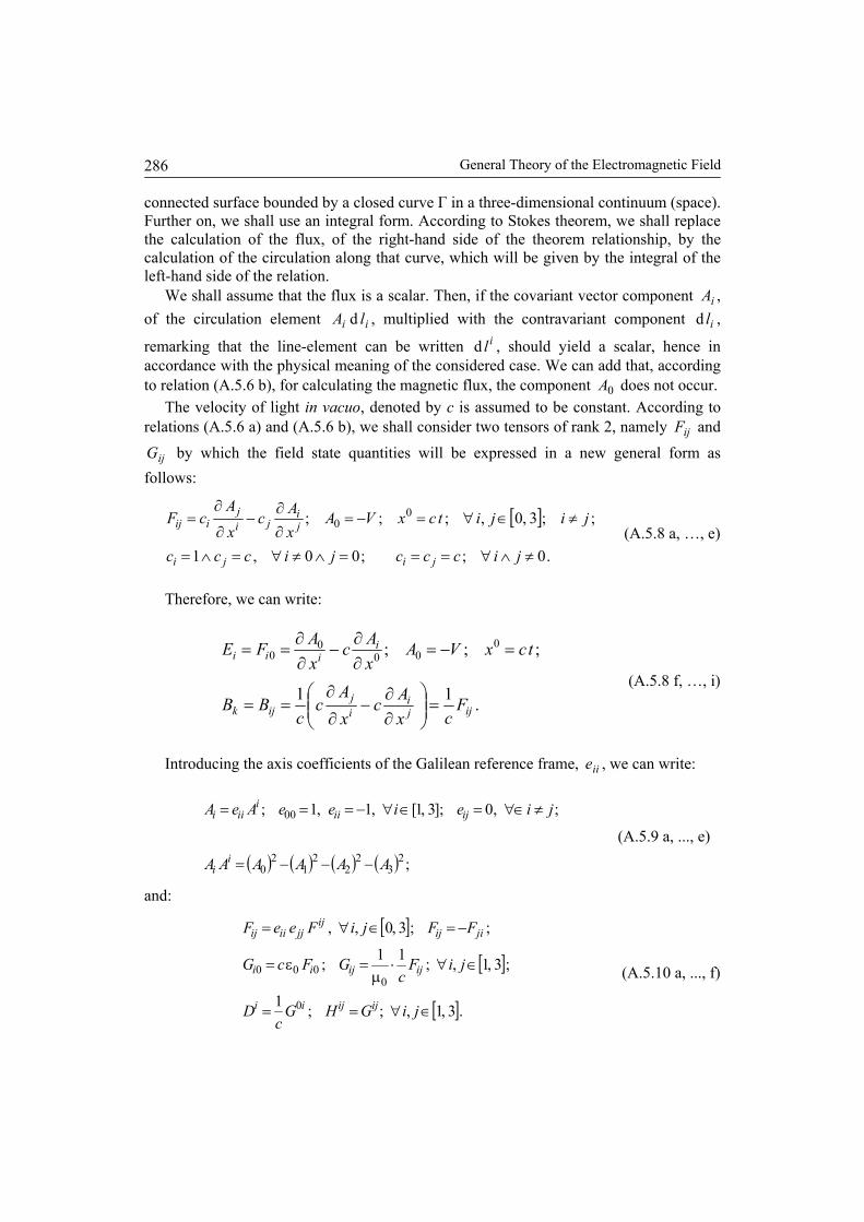
General Theory of the Electromagnetic Field
286
connected surface bounded by a closed curve Γ in a three-dimensional continuum (space). Further on, we shall use an integral form. According to Stokes theorem, we shall replace the calculation of the flux, of the right-hand side of the theorem relationship, by the calculation of the circulation along that curve, which will be given by the integral of the left-hand side of the relation.
We shall assume that the flux is a scalar. Then, if the covariant vector component iA , of the circulation element ii lA d , multiplied with the contravariant component ild ,
remarking that the line-element can be written ild , should yield a scalar, hence in accordance with the physical meaning of the considered case. We can add that, according to relation (A.5.6 b), for calculating the magnetic flux, the component 0A does not occur.
The velocity of light in vacuo, denoted by c is assumed to be constant. According to relations (A.5.6 a) and (A.5.6 b), we shall consider two tensors of rank 2, namely ijF and
ijG by which the field state quantities will be expressed in a new general form as follows:
[ ]
.0;;00,1
;;3,0,;;; 00
≠∧∀===∧≠∀=∧=
≠∈∀=−=∂∂
−∂
∂=
jicccjiccc
jijitcxVAxAc
xA
cF
jiji
ji
jij
iij (A.5.8 a, …, e)
Therefore, we can write:
.11
;;; 000
00
ijji
ij
ijk
iiii
Fcx
AcxA
cc
BB
tcxVAxAc
xAFE
=⎟⎟⎠
⎞⎜⎜⎝
⎛∂∂
−∂
∂==
=−=∂∂
−∂∂
==
(A.5.8 f, …, i)
Introducing the axis coefficients of the Galilean reference frame, iie , we can write:
( ) ( ) ( ) ( ) ;
;,0;]3,1[,1,1;
23
22
21
20
00
AAAAAA
jieieeAeA
ii
ijiii
iii
−−−=
≠∈∀=∈∀−===
(A.5.9 a, ..., e)
and:
[ ]
[ ]
[ ].3,1,;;1
;3,1,;11;
;;3,0,,
0
0000
∈∀==
∈∀⋅µ
=ε=
−=∈∀=
jiGHGc
D
jiFc
GFcG
FFjiFeeF
ijijii
ijijii
jiijij
jjiiij
(A.5.10 a, ..., f)
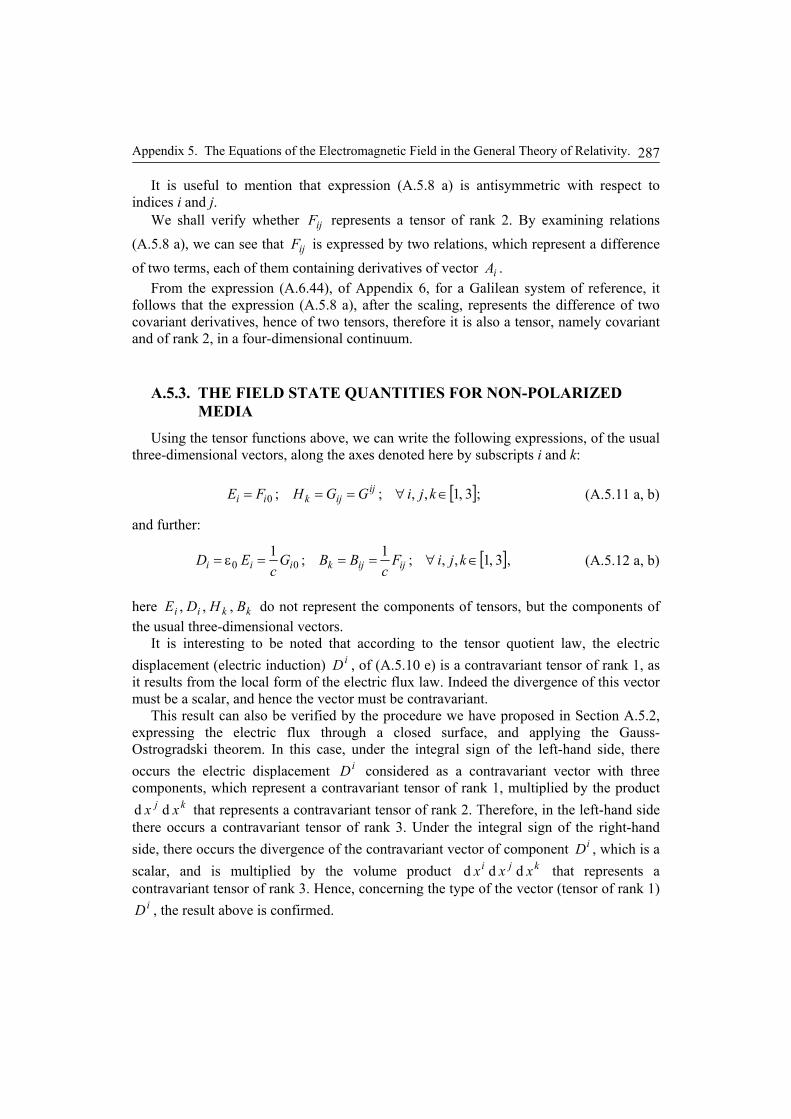
Appendix 5. The Equations of the Electromagnetic Field in the General Theory of Relativity.
287
It is useful to mention that expression (A.5.8 a) is antisymmetric with respect to indices i and j. We shall verify whether ijF represents a tensor of rank 2. By examining relations (A.5.8 a), we can see that ijF is expressed by two relations, which represent a difference of two terms, each of them containing derivatives of vector iA . From the expression (A.6.44), of Appendix 6, for a Galilean system of reference, it follows that the expression (A.5.8 a), after the scaling, represents the difference of two covariant derivatives, hence of two tensors, therefore it is also a tensor, namely covariant and of rank 2, in a four-dimensional continuum.
A.5.3. THE FIELD STATE QUANTITIES FOR NON-POLARIZED
MEDIA
Using the tensor functions above, we can write the following expressions, of the usual three-dimensional vectors, along the axes denoted here by subscripts i and k:
[ ];3,1,,;;0 ∈∀=== kjiGGHFE ijijkii (A.5.11 a, b)
and further:
[ ],3,1,,;1;100 ∈∀===ε= kjiF
cBBG
cED ijijkiii (A.5.12 a, b)
here kkii BHDE ,,, do not represent the components of tensors, but the components of the usual three-dimensional vectors.
It is interesting to be noted that according to the tensor quotient law, the electric displacement (electric induction) iD , of (A.5.10 e) is a contravariant tensor of rank 1, as it results from the local form of the electric flux law. Indeed the divergence of this vector must be a scalar, and hence the vector must be contravariant.
This result can also be verified by the procedure we have proposed in Section A.5.2, expressing the electric flux through a closed surface, and applying the Gauss-Ostrogradski theorem. In this case, under the integral sign of the left-hand side, there occurs the electric displacement iD considered as a contravariant vector with three components, which represent a contravariant tensor of rank 1, multiplied by the product
kj xx dd that represents a contravariant tensor of rank 2. Therefore, in the left-hand side there occurs a contravariant tensor of rank 3. Under the integral sign of the right-hand side, there occurs the divergence of the contravariant vector of component iD , which is a scalar, and is multiplied by the volume product kji xxx ddd that represents a contravariant tensor of rank 3. Hence, concerning the type of the vector (tensor of rank 1)
iD , the result above is confirmed.

General Theory of the Electromagnetic Field
288
For the vector electric induction to be contravariant, it is necessary that the covariant vector (tensor of rank 1) iE be multiplied by a contravariant tensor of the second rank. We can write:
[ ] .,3,1,,0ijij
jiji ejiED =δ∈∀εδ= (A.5.13 a, b)
It is to be noted that the tensor iD is defined using a four-dimensional space, but it has only three components, because the components (elements) of tensor ijF are zero for the components of which the two indices are equal to each other, hence for the time co-ordinate, i.e., for 0=i .
The relations (A.5.10 a, e), (A.5.8 c) yield the following tensor relations:
[ ].3,1;; ∈∀−=−= iEEDD iii
i (A.5.14 a, b)
The expressions of iE , and kB , from relation (A.5.11 a) and (A.5.12 b), respectively, are valid for vacuum as well as for polarized media, while the expressions of iD and kH , from the (A.5.12 a) and (A.5.11 b), are valid only for vacuum.
A.5.4. THE FIELD AND SUBSTANCE STATE QUANTITIES FOR POLARIZED MEDIA
For a polarized medium, the substance state quantities of electric and magnetic polarization, respectively, have to be introduced by symbols P and JM , where we have used the index J in order to avoid any confusion with index j above. In this Section, we shall consider only the temporary polarization. In addition, we shall indicate in this Section, the components of the usual three-dimensional vectors by index k denoting one of the three axes. In this case, the respective quantities can be introduced by the following relations:
[ ],3,1,,;;;
;;;
0,J,me,0 ∈∀µ=χ=χε=
===
kjiMMHMEP
HHMMPP
kkjkjkjkjk
ijk
ijk
ik (A.5.15 a, …, f)
where in relations from a to c, in the left-hand side, the usual vector components are written, but in the right-hand side, the tensor components are written; while in relations from d to f, in both sides, only usual vector components are written. In this manner, the components of tensors may be expressed more easily. It follows:
[ ],3,1,,;; ,J0e00 ∈∀+µ==χε+δε= kjiMHBBEED kkijkjij
jiji (A.5.16 a, b)
where jE may represent the usual vector component as well as the tensor component, and ijB , and kB represent the tensor component, and the corresponding vector component, respectively.
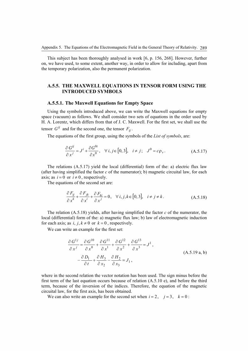
Appendix 5. The Equations of the Electromagnetic Field in the General Theory of Relativity.
289
This subject has been thoroughly analysed in work [6, p. 156, 268]. However, further on, we have used, to some extent, another way, in order to allow for including, apart from the temporary polarization, also the permanent polarization.
A.5.5. THE MAXWELL EQUATIONS IN TENSOR FORM USING THE INTRODUCED SYMBOLS
A.5.5.1. The Maxwell Equations for Empty Space
Using the symbols introduced above, we can write the Maxwell equations for empty space (vacuum) as follows. We shall consider two sets of equations in the order used by H. A. Lorentz, which differs from that of J. C. Maxwell. For the first set, we shall use the tensor ijG and for the second one, the tensor ijF .
The equations of the first group, using the symbols of the List of symbols, are:
[ ] .;,3,0,, 00
0
v
ii
j
ijcJjiji
xGJ
xG
ρ=≠∈∀∂∂
+=∂∂ (A.5.17)
The relations (A.5.17) yield the local (differential) form of the: a) electric flux law (after having simplified the factor c of the numerator); b) magnetic circuital law, for each axis; as 0=i or 0≠i , respectively.
The equations of the second set are:
[ ] .,3,0,,,0 kjikjixF
x
F
x
Fj
kiijk
kij ≠≠∈∀=
∂∂
+∂
∂+
∂
∂ (A.5.18)
The relation (A.5.18) yields, after having simplified the factor c of the numerator, the local (differential) form of the: a) magnetic flux law; b) law of electromagnetic induction for each axis; as 0,, ≠kji or 0=k , respectively.
We can write an example for the first set:
,
,
13
2
2
31
13
13
2
12
1
11
0
101
JxH
xH
tD
Jx
Gx
Gx
Gx
Gx
Gj
j
=∂∂
−∂∂
+∂
∂−
=∂
∂+
∂
∂+
∂
∂+
∂
∂=
∂
∂
(A.5.19 a, b)
where in the second relation the vector notation has been used. The sign minus before the first term of the last equation occurs because of relation (A.5.10 e), and before the third term, because of the inversion of the indices. Therefore, the equation of the magnetic circuital law, for the first axis, has been obtained.
We can also write an example for the second set when 0,3,2 === kji :

General Theory of the Electromagnetic Field
290
,0
,0
3
2
2
31
302
230
023
=∂∂
−∂∂
+∂
∂
=∂
∂+
∂
∂+
∂
∂
xE
xE
tB
xF
xF
xF
(A.5.20 a, b)
where in the second relation the vector notation has been used. The last equation has been obtained after having simplified the factor c of the numerator.
Therefore, the local (differential) form of the local (differential) equation of the law of electromagnetic induction, for the first axis, has been obtained.
A.5.5.2. The Maxwell Equations for Polarized Media
In order to consider the equations for polarized media, it is necessary to introduce the polarization tensors of the substance.
For the first set of equations, we shall complete relations of (A.5.17), according to relations (A.5.15 a, b). In order to bring the equation of the first set into a covariant form, with respect to any change of co-ordinates, we shall introduce, in the equation above, the symbols:
[ ];3,1,: 000 ∈∀+δε=+= jPcEcPcGG j
jjjjjj (A.5.21)
[ ];3,1,: 00 ∈∀−δε−= iPcEcG i
iiii (A.5.22)
[ ];3,1,,: ∈∀−= jiMGG ijijij (A.5.23)
[ ].3,1;0;0; 000 ∈∀==ρ= jMPcJ jv (A.5.24 a, b, c)
In all definition formulae above, the terms of the form ijG from the right-hand side are those given by relations (A.5.10 c, d). Consequently, equation (A.5.17) becomes:
[ ] .0;0;;,3,0,, 000 ==ρ=≠∈∀=∂∂ j
vi
j
ijMPcJjijiJ
xG (A.5.25 a, …, d)
The equations of (A.5.25) correspond to equations of (A.5.17) above. For the second set of equations, we shall obtain the same relations as for non-polarized
media because the occurring quantities are not influenced by considering the polarization:
[ ] .,3,0,,0 kjijixF
x
F
x
Fj
kiijk
kij ≠≠∈∀=
∂∂
+∂
∂+
∂
∂ (A.5.26)
The equation (A.5.26) corresponds to equation (A.5.18) above.
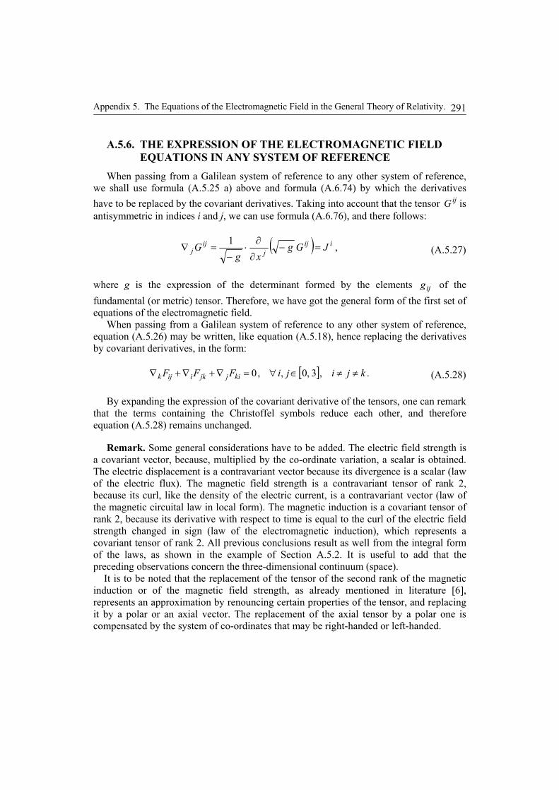
Appendix 5. The Equations of the Electromagnetic Field in the General Theory of Relativity.
291
A.5.6. THE EXPRESSION OF THE ELECTROMAGNETIC FIELD
EQUATIONS IN ANY SYSTEM OF REFERENCE
When passing from a Galilean system of reference to any other system of reference, we shall use formula (A.5.25 a) above and formula (A.6.74) by which the derivatives have to be replaced by the covariant derivatives. Taking into account that the tensor ijG is antisymmetric in indices i and j, we can use formula (A.6.76), and there follows:
( ) ,1 iijj
ijj JGg
xgG =−
∂
∂⋅
−=∇ (A.5.27)
where g is the expression of the determinant formed by the elements ijg of the fundamental (or metric) tensor. Therefore, we have got the general form of the first set of equations of the electromagnetic field.
When passing from a Galilean system of reference to any other system of reference, equation (A.5.26) may be written, like equation (A.5.18), hence replacing the derivatives by covariant derivatives, in the form:
[ ] .,3,0,,0 kjijiFFF kijjkiijk ≠≠∈∀=∇+∇+∇ (A.5.28)
By expanding the expression of the covariant derivative of the tensors, one can remark that the terms containing the Christoffel symbols reduce each other, and therefore equation (A.5.28) remains unchanged.
Remark. Some general considerations have to be added. The electric field strength is a covariant vector, because, multiplied by the co-ordinate variation, a scalar is obtained. The electric displacement is a contravariant vector because its divergence is a scalar (law of the electric flux). The magnetic field strength is a contravariant tensor of rank 2, because its curl, like the density of the electric current, is a contravariant vector (law of the magnetic circuital law in local form). The magnetic induction is a covariant tensor of rank 2, because its derivative with respect to time is equal to the curl of the electric field strength changed in sign (law of the electromagnetic induction), which represents a covariant tensor of rank 2. All previous conclusions result as well from the integral form of the laws, as shown in the example of Section A.5.2. It is useful to add that the preceding observations concern the three-dimensional continuum (space).
It is to be noted that the replacement of the tensor of the second rank of the magnetic induction or of the magnetic field strength, as already mentioned in literature [6], represents an approximation by renouncing certain properties of the tensor, and replacing it by a polar or an axial vector. The replacement of the axial tensor by a polar one is compensated by the system of co-ordinates that may be right-handed or left-handed.

General Theory of the Electromagnetic Field
292
List of Symbols Used in Appendix 5
iA – component of the four-vector potential; c – velocity of light in empty space, supposed to be constant;
iD – component of the electric displacement, considered as a usual three-dimensional vector;
iD – contravariant component of the electric displacement;
iie – axis coefficient, for the axis i of the Galilean reference frame, i.e., element of the fundamental tensor of this frame;
iE – covariant component of the electric field strength, as well as component of the electric field strength along axis i as a usual three-dimensional vector;
iE – contravariant component of the electric field strength;
ijF – component of the covariant tensor of rank 2 yielding ijB ;
0iF – component of a covariant tensor, deriving from the previous one, and yielding the component iE of the electric field strength, considered as a usual three-dimensional vector;
g – value of the determinant of the fundamental tensor; ijG – contravariant tensor of rank 2, and yielding ijH ;
ijG – covariant tensor of rank 2, and yielding kH ;
00 ,ii
G
G
– covariant and contravariant components, deriving from the previous one, and yielding the component iD ;
kH – component of the magnetic field strength along axis k , considered as a usual three-dimensional vector;
ii JJ , – component of a contravariant four-vector representing the density of the
conduction electric current, along axis i , and of the usual three-dimensional vector, respectively;
ijM – component of a contravariant tensor of rank 2, yielding kM ;
kM – magnetisation along axis k, while the magnetic polarization is kM J , considered as a usual three-dimensional vector;
iP – contravariant component of the electric polarization;
kP – electric polarization along axis k , considered as a usual three-dimensional vector;
V – electric potential; ix – co-ordinate along axis i ;
ijij δδ ,
– symbols equal to unity for equal indices, and equal to zero for different ones (Kronecker symbols);
ε – electric permittivity, in vacuo it is 0ε ; µ – magnetic permeability, in vacuo it is 0µ ;
vρ – volume density of the electric free charge; χ – electric and magnetic susceptibility, according to the index e or m.

Appendix 5. The Equations of the Electromagnetic Field in the General Theory of Relativity.
293
REFERENCES 1. EINSTEIN, A.: The Meaning of Relativity. Princeton University Press, Princeton, New
Jersey, 1955. Teoria relativităţii. Editura Tehnică, Bucureşti, 1957. 2. LANDAU, L., LIFCHITZ, E.: Théorie des champs. Éditions Mir, Moscou, 1970. 3. FOCK, V.A.: The Theorie of Space, Time and Gravitation, (translated by N. Kemmer).
Pergamon Press, London, 1959. Teoria spaţiului timpului şi gravitaţiei. Ed. Academiei Române, Bucureşti, 1962.
4. ARZELIES, H.: Électricité. Le point de vue macroscopique et relativiste. Gauthier-Villars, Éditeur, Paris, 1963.
5. PATHRIA, R.K.: The theory of relativity. Second edition, Pergamon Press, Oxford, New York, Toronto, Hindustan Publishing Corporation (India), Delhi, 1974.
6. FOURNET, G.: Électromagnétisme à partir des équations locales. Masson et C-ie, Éditeurs, Paris, 1985.
7. LUDVIGSEN, M.: La relativité générale. Une approche géométrique. Dunod, Paris, 2000. 8. NICOLAIDE, A.: Considerations on the energy-momentum tensor in the special and general
theory of relativity. Rev. Roum. Sci. Techn. – Électrotechn. et Énerg., 2006, 51, 4, pp. 405–417.
9. NICOLAIDE, A.: Considerations on the covariant form of the equations of the electromagnetic field in polarized media. Rev. Roum. Sci. Techn. – Électrotechn. et Énerg., 2008, 53, 1, pp. 11–22.
10. KOCHIN, N.E.: Vector calculus and introduction to tensor calculus. Seventh edition. Publishing House of the Academy of Sciences, Moscow, 1951. KOCIN, N.E.: Calculul vectorial şi introducere în calculul tensorial. Edit. Tehnică, Bucureşti, 1954.
11. DOUBROVINE, B.A., NOVIKOV, S.P., FOMENKO, A.T.: Géométrie contemporaine. Méthodes et applications. Première partie. Éditions Mir, Moscou, 1985.
12. **
* Prove that 4 vector potential is really a vector. 16 messages, 6 authors. www.physicsforums.com/archive/index.php/t-232693.html - 83 k; 27th Oct., 2008.

General Theory of the Electromagnetic Field
294
APPENDIX 6
TENSOR CALCULUS
In this Appendix, we shall recall certain definitions and several largely used relations. In addition, certain more important proofs will be given. The bibliographic mentions [1]-[14] specific for this Appendix are at the end of this Appendix. Also, a List of symbols is given at the end of this Appendix. We shall have in view the works [8], [9] that present certain advantages for the applications.
A.6.1. TENSOR ALGEBRA
The Vector Calculus aims to renounce the systems of co-ordinates, by using vectors, which are oriented straight-line segments. The various operations over vectors can be performed without resorting to co-ordinates. In the case of more complicated objects, when the number of co-ordinates is greater than number three, the use of vectors does not suffice. For this reason, it is necessary to use systems of co-ordinates (systems of reference, reference frames) [3, p. 25], [14, p. 6], and tensors instead of vectors.
A.6.1.1. Systems of Co-ordinates
The simplest system of co-ordinates, in the three-dimensional space, is the Cartesian system of co-ordinates. The considered system is orthogonal and will be chosen right-handed. In general, any system of co-ordinates may be used, according to the scope. In the Theory of Relativity, taking in view that each event is characterized by its position in space and moment in time, a four-dimensional system of co-ordinates is to be used, and the corresponding space is called four-dimensional space, four-dimensional continuum or space-time continuum. In general, an n-dimensional continuum may be considered. The co-ordinates in this continuum are also called Gaussian co-ordinates.
When passing from a system of co-ordinates to another, the co-ordinates of the first will be denoted by ix , and those of the second by ix′ , hence adding the sign prime. The quantities referring to the second system will also be indicated by the sign prime. The index i written as superscript can take every value of the numbers denoting the co-ordinates. In accordance with several well-known works, in the case of the Theory of Relativity, we shall count the axes of co-ordinates starting with zero (for time). For any different case, we shall make mention. The relationship between the co-ordinates of the second system will be expressed in terms of those of the first one. The following relation will be used:
( ) .,,, 3210 xxxxxx ii =′ (A.6.1)

General Theory of the Electromagnetic Field 296
The transformation function (A.6.1) must be continuous, and its derivatives of the first three orders should also be continuous. In addition, the Jacobian determinant must be different from zero, for the inverse transformation to be possible.
Sometimes, it may occur that the number of axes of co-ordinates of the first system, say a Cartesian one, is greater than that of the second system.
According to the previous assumptions, the total differential of the function given by (A.6.1) is:
.3,0,
,dddddd 33
22
11
00
ji
xx
xx
x
xx
x
xx
x
xx
x
xx j
j
iiiiii
(A.6.2 a)
As a result, one may write:
.3,0,,dd jixax jij
i (A.6.2 b)
A.6.1.2. Tensors of Rank 0 and of Rank 1. Summation Convention. Covariant and Contravariant Tensors. Affine transformations.
In order to fix the ideas, we consider the case where n co-ordinates are necessary. The corresponding space is called an n-dimensional space or an n-dimensional continuum. We are going to recall that a set containing, for each point of the space, only a scalar, is called a tensor of rank (also called order) zero. A set containing, for each point of the space, nquantities may constitute a vector also called a tensor of rank 1. Any set of n quantities may represent a tensor of rank (order) 1, also called vector, but for to be a tensor (vector), the set elements must change, when passing (switching) from the first system of co-ordinates to the second one, according to formulae below:
,1,0,;; njiAaAAaA jj
iiji
ji (A.6.3 a, b)
or
njiAaAAaA jj
iiji
ji ,1,;; , (A.6.4 a, b)
depending on the number attributed to the first axis. We shall use various formulae. A set of quantities satisfying a relation of the form (A.6.3 b) is represented by the
differentials of the co-ordinates as in relations (A.6.2 b). In order to simplify the relations, certain authors denote the co-ordinates of the first
system of reference, in the case in which it is a Cartesian system, by iy and those of the
second system by ix , hence renouncing the sign prime, what we also shall do, when the case occurs.
In relations (A.6.2) – (A.6.4), and further on, the summation convention is used, namely, if in a term, an index occurs twice, as subscript and superscript, respectively, or if two factors of the same term have the same index, regardless of their position (subscript
Appendix 6. Tensor Calculus. 297
or superscript), it implies the summation of the terms obtained for all values that the respective index can take.
The coefficients of the last relations (A.6.3), (A.6.4), may be expressed as follows:
.0det;; iji
jj
ij
iij a
x
xa
x
xa (A.6.5 a, b)
Among the various possible transformations, one can mention the affine transformation and the orthogonal transformation, due to their respective properties. The affine transformation preserves co-linearity and ratios of distances. Therefore, in an affine transformation all points lying on a line (e.g., a straight-line) remain on the same line after transformation. Also, the ratio between the lengths of two portions of a straight-line segment keeps the same value after transformation. The affine transformations are linear transformations. An affine transformation may be composed of: translation, scaling, rotation, shearing and reflection. However the angle between lines may change. The orthogonal transformations, also called orthonormal transformations, preserve the length of vectors and the angles between them. It may be composed only by rotation or rotation and reflection.
For an orthogonal transformation, the coefficients appearing in (A.6.5) must satisfy the relation:
,1det ija (A.6.6)
where the transformation for which the plus or minus sign occurs is called a proper or improper transformation, respectively.
In any relation with tensors correctly written, when suppressing the indices denoted by the same letters, and occurring as subscript and superscript, respectively, in each of the two sides of the relation, the remaining indices in each side will be the same.
According to the general convention, if the components of a tensor change according to formulae of type (A.6.3 a), we deal with a contravariant tensor (with respect to this index), whereas if we consider formulae of type (A.6.3 b), we now deal with a covariant
tensor. Each index with respect to which the tensor is contravariant is written as superscript, and each one with respect to which the tensor is covariant is a subscript. For this reason, the co-ordinates are denoted by using superscripts (except some authors who prefer to keep for co-ordinates the index as subscript, in order to avoid the usage of parentheses in the case of exponents (powers), but they mention this fact as unusual).
In the case of the translation, when passing from a Cartesian system of co-ordinates to another one of the same type, translated and rotated with respect to the former one, the coefficients of relations (A.6.5 a) and (A.6.5 b), are equal. Consequently, then no difference appears between the covariant and contravariant tensors. It is an orthogonal transformation. In the case of the Cartesian systems of the Special Theory of Relativity, which represent Galilean systems of reference, the Lorentz transformation is orthogonal, but it is to be noted that the field state quantities do not change like the co-ordinates or inversely, because they do not represent four-dimensional vectors.
General Theory of the Electromagnetic Field 298
A.6.1.3. Operations with Tensors. Tensors of Rank 2.
In order to fix the ideas, further on, we shall consider a four-dimensional space, and precise some important operations.
1° Addition. The sum of two tensors of rank 1 may be seen in the example:
3,0; iBAC iii , (A.6.7)
where the values taken by the index i are also given, so that one finally obtains 4 relations. The relation above is not casual and corresponds to the addition of the components of two vectors. As a result the sum of two tensors is also a tensor.
2° Multiplication. The product of two tensors of rank 1 may be seen in the next example:
.3,0,; jiBAC jiij (A.6.8)
The following components (elements) will be obtained for the indices 0i and 1i :
.3,0,;;;;
;;;;
3113211211110110
3003200210010000
jiBACBACBACBAC
BACBACBACBAC(A.6.9)
Similarly, we can write the components for the other values of the index i. Finally, 16 scalar values will be obtained. In this case, it is necessary to use in the left-hand side two indices for obtaining a suggestive representation of all obtained elements. Therefore, we
shall obtain a set of 24 quantities, which may be a tensor of rank (order) 2, and the symbol of the general term (that may also be called component or element) of the tensor will have two indices. In this case, the expression of the general term of the tensor, when passing from the first to the second system of reference is:
klj
l
i
k
lkj
l
i
k
lj
l
ki
k
jiij Cx
x
x
xBA
x
x
x
xB
x
xA
x
xBAC , (A.6.10)
which, as further shown, is a twice covariant tensor. There follows that the values of the components of the tensor will change when passing from a reference system to another one, according to the transformation relation, as for the co-ordinates if the respective index is contravariant, and inversely if the index is covariant. As shown in the last relation, if the letter of a certain index appearing twice, may lead to a confusion, it is convenient to replace it by another letter, as we did, because if the index takes the same values, the result will be not affected. From the previous example, there follows that the product of two tensors, in general, depends on the order of factors.
Appendix 6. Tensor Calculus. 299
3° Tensors of rank 2 (Tensors of the second order). Tensors of higher rank.
According to relation (A.6.10), a set containing 2n quantities (first condition) may be a tensor of rank 2 in an n-dimensional continuum, whether when passing from the first system of reference to the second, the general term will change according with the character of the respective index contravariant or covariant (second condition), like to the co-ordinates or conversely. The form of the general term of a rank 2-tensor shows one of
the following forms: ji
ijij TTT ,, , namely twice covariant, twice contravariant, mixed
once covariant and once contravariant. If the tensor is written as a matrix, the letters i and j denote the row and column, respectively. Other symbols have been proposed in [7].
Any tensor ijC is called symmetric or antisymmetric, in its indices i and j, as the
relation jiij CC or jiij CC , respectively, is fulfilled [5, p. 69]. An antisymmetric
tensor can be built up by the relation:
3,1,, jiBABAC ijjiij . (A.6.11)
By examining this tensor, we can see that it has 9 components, and only 6 are different from zero, the terms with the same double index being zero. From these 6 terms, three of them differ from the other three only in sign. Considering three components, we can see that they just represent the components of the vector product of two three-dimensional vectors.
Any tensor of rank 2, say ijT may be considered as constituted of two tensors: one
symmetric ijS , and another antisymmetric ijA , as follows:
.;2
1;
2
1ijijijjiijijjiijij ASTTTATTS (A.6.12)
Similarly, we can write the general term of a tensor several times covariant and
several times contravariant, for instance uvijkT , which represents the general term of a
tensor of rank 5, three times covariant and twice contravariant.
4° Equality of two tensors. Two tensors, ijA and ijB are equal to each other if each
element of one is equal to the corresponding element of the other:
NjiBA ijij ,, . (A.6.13)
This property of the tensors is invariant, because if this property is fulfilled in a system of reference, it holds in any other system of reference. Consequently, if the components (elements) of a tensor are zero in one system of reference, they will also be zero in any other system of reference.
5° Contraction of a tensor. The operation results from the following example. Let iA
and jB be two tensors, their product will be ji
ji BAC . If one puts ji , the result
will be:
General Theory of the Electromagnetic Field 300
3,1,33
22
11 jiBABABABABA i
jj
i , (A.6.14)
which just represents the scalar product of vectors iA and jB . The contracted result will be, in this case, a scalar. If the tensors of the product were of higher rank, then the result, after the contraction on an index, will lead to a tensor of a rank smaller of two unities. This operation is called contraction on an index, in the previous case on index i.
6° Tensors of higher ranks. The rank or order of a tensor is equal to the number of indices. All operations explained above are valid regardless of the rank of the considered tensors. It is useful to add that if a set of quantities multiplied with a tensor of rank p yields a tensor of rank qp , then, the set will be a tensor of rank q. This rule is called the quotient law [5, p. 71], or more generally, the theorem of tensor classification
[10, p. 376].
7° Covariant equation. Another remark concerns the equations. In Physics, an equation must keep the same form when passing from a Cartesian system of co-ordinates to another one. This property is expressed saying that the equation is covariant with respect to the transformation of the co-ordinates. The property is called covariance of the
equation with respect to the transformation of co-ordinates. This property may be extended to any system of co-ordinates. We should add that in this case, the meaning of the word covariant is different from the meaning concerning the type of a tensor.
A.6.2. TENSOR ANALYSIS
A.6.2.1. The Metrics of a Space
The metrics of a space represents, in fact, the expression of the distance between two points very near to each other. The expression may have different forms. In the case of the three-dimensional space (Euclidean Geometry), in a Cartesian system of reference, the expression will be:
2322212 dddd xxxs . (A.6.15)
Also in the case of a Cartesian system of co-ordinates, but with four dimensions, in the Theory of Relativity, the following metric relation is used:
3,1,1;1;,0;3,0,ddd 002
ieejieixxes iiijji
ij . (A.6.16)
A system of reference the metrics coefficients of which are given by relations (A.6.16) is called Galilean system of reference.

Appendix 6. Tensor Calculus. 301
A.6.2.2. The Fundamental Tensor. General Systems of Co-ordinates.
We shall consider anew two systems of co-ordinates, the first being a Cartesian system, like above, and the second any curvilinear system. In this case, we shall denote,
as mentioned after formula (A.6.4), the co-ordinates of the first system by iy , and those
of the second by ix . We want to express the transformation of the metric relation in the second system. The metric relation is assumed invariant when changing the system of co-ordinates. Indeed, the distance between two points must be the same, regardless of the system of co-ordinates. Therefore, we shall equate the metric relation expressed in the two systems. We here consider the case with four co-ordinates used in the Special and General Theory of Relativity. The following quadratic form may be written as follows:
.3,0,,dddd
2222
kixx
yexaeyes k
k
i
iiki
kiii
ii (A.6.17)
Expanding the terms of the preceding equation, we shall get:
3,0,,,ddd 2lkixx
x
y
x
yes lk
l
i
k
i
ii . (A.6.18)
The relation (A.6.18) may be written in one of the forms:
;3,1,,dddd2ddd
;3,0,,ddd
00
0000
2
2
xxgxxgxxgs
jixxgs jiij
(A.6.19 a, b)
which is a quadratic form, called fundamental form of the metrics, and contains the following quantities:
;,0,0
Na
aj
a
ia
j
a
i
a
aajiij Nax
y
x
y
x
y
x
yegg (A.6.20)
where 1N represents the number of axes of co-ordinates of the first system. If the numbering of axes began with 1, then the index zero would be replaced by 1, and N will be the number of axes of the first system. The set of elements ijg represents a tensor called the fundamental tensor. Indeed, it
fulfils the first condition from 3º of A.6.1.3, containing 16 components (elements), thus 2n elements in a space with 4n dimensions. Concerning the second condition from 3º
of A.6.1.3, we shall remark what follows. In relation (A.6.19), the product ji xx dd ,which is the product of two contravariant tensors of rank 1, represents a contravariant
General Theory of the Electromagnetic Field 302
tensor of rank 2. The product of this tensor with the tensor ijg yields a scalar, namely the
left-hand side of the equation, therefore the set ijg represents a covariant tensor of rank 2.
In the case of a Cartesian system of co-ordinates, these quantities become:
;,0;3,1,1;100 jigigg ijii (A.6.20 a)
where ijij eg , and then the quadratic form (A.6.19) takes the form of the expression in
(A.6.17) after the first equal sign, and is called normal or quasi-Euclidean form of the
metrics of the considered space. If no confusion occurs it may be written ix instead of iy . The quantities ije may also be called axis coefficients.
If a quadratic form has the coefficients ijg different from those of formulae
(A.6.20 a), it is called a Riemannian form of the metric relation of the space defined by
the co-ordinates ix . If the fundamental quadratic form of any space cannot be reduced to the form having the components of formulae (A.6.20 a), that space is considered, by analogy with the theory of surfaces, as having a curvature [10], [11].
A.6.2.3. Relations between Covariant and Contravariant Vectors
Consider as given any covariant vector iA . We are now looking for the relation between a covariant vector and a contravariant one, in any n-dimensional continuum (space). It is possible to obtain a contravariant vector from the covariant one, by using the following relation:
njiAgA jiji ,0,, . (A.6.21)
The components of the contravariant vector can be obtained by solving the system of equations (A.6.21). One obtains:
ij
ijji
i
ijj ggnji
g
DgA
g
DA det;,0,,, , (A.6.22)
where the quantities of the form jiD are cofactors (minors) corresponding to the element ij, of the determinant D of the quadratic fundamental form made of elements ijg .
Similarly, we can write:
njiAgA ijij ,0,, . (A.6.23)
The operations represented by relation (A.6.21) and (A.6.23), respectively, may be referred to as lowering and raising an index, respectively [5, p. 173]. By replacing expression (A.6.22) into (A.6.23), it results that:

Appendix 6. Tensor Calculus. 303
njig
DgAgA
g
D ijji
iji
i
ij
,0,;; , (A.6.24)
and, if changing the order of indices, the tensor ijg being symmetric in i and j we get:
g
Dgg
jijiij . (A.6.25)
If considered as matrices, ijg and ije are the inverse of ijg and ije . Hence ijij ee .
Similarly, one can transform the character of a tensor, say a contravariant tensor of
rank 2, denoted ijT , by lowering one index. For this purpose, we multiply the tensor with the element kug of the fundamental tensor, and we shall contract on indices i and u, by putting ui , as follows:
jkku
ij TgT , (A.6.26)
and a half-height dot was placed instead of the index which vanished, in order to show the places of indices on which the tensor was contracted. These dots are used in cases in which, for any reason, this mention is required or useful. We obtained a mixed tensor, once covariant and once contravariant. The same transformation may appear in the form:
jkki
ij TgT . (A.6.27)
In the case of a Galilean (also called quasi-Euclidean) system of reference, several simple relationships can be obtained, as follows:
,,0;3,1,1,1
;
;
00 jieiee
TeTeT
TeeTeeT
ijii
ijii
sjsi
ji
ijjjii
qsjsiqij
(A.6.27 a-e)
where, for simplicity we omitted the signs dot.
A.6.2.4. Relations between the Components of the Fundamental Tensor
1° First relation. Consider the term below:
jkik
ji ggg . (A.6.28)
This relation may be obtained from:
jj
ijjk
ikijjkkk
iki AgAggAAgAAgA ;; . (A.6.29)
General Theory of the Electromagnetic Field 304
In order to get ji AA , it follows that in relation (A.6.29) the coefficient of the last
right-hand side should be:
jigjigj
ij
i ,1;,0 . (A.6.30)
2° Second relation. Consider the product below, where the indices j and k do not vary. One will get:
kj
nknj
kj
kj
ikij ggggggggg ...2
21
1 . (A.6.31)
3° Third relation. We shall consider the product above, but we shall put kj . Then, we can start from the result above, and j can take successively n values, and for each value, that product can be different from zero, and thus equal to unity, only if the two indices are equal to each other, hence n times. One immediately obtains:
ngggjj
ijij . (A.6.32)
4° Kronecker symbols. Related to the relations above, the symbols ji
ijij ,, , also
called Kronecker symbols, have also to be considered. Each of this symbols has the property to have the value zero if ji , and the value 1 if ji . Therefore, we can write
ijij e . The sets ijg , ije and ij are tensors of rank 2, twice covariant.
A.6.3. THE LENGTH OF A VECTOR IN ANY SYSTEM OF REFERENCE
In order to express the length of a vector iA at any point, in any system of reference, one can refer to relation (A.6.19), which expresses the square of the element of length. The components of the considered vector being along the tangents of the lines of co-ordinates supposed translated at that point, the use of the mentioned relation is justified. Therefore, the length will be obtained from the following relation:
ii
jj
jiij AAAAAAgA2 , (A.6.33)
which is like the square of the modulus of a vector in the three-dimensional space.
The angle between two vectors iA and jB can be expressed, on similar bases, as follows:
ii
ii
iiji
BBAA
BABA ,cos . (A.6.34)

Appendix 6. Tensor Calculus. 305
A.6.4. COVARIANT DERIVATIVE OF A COVARIANT VECTOR
For the sake of clarity, we shall present a simple deduction of the covariant derivative of a covariant vector, avoiding several extensions used in literature, like the parallel transport of a vector, gradient of an alternative vector, and other considerations. Nevertheless, we shall obtain the same results necessary for calculations.
Let us consider two systems of reference denoted by GK (Galilean system) with
1N dimensions (the first dimension being denoted by zero and the last by N), and by K, any inertial or non-inertial system of reference with four dimensions. In the former
one, the co-ordinates will be denoted by iy and in the latter one, by ix . Also, let us consider one covariant four-vector, denoted in the former system of reference frame by
iY and in the latter by iA . The relation between the vector components is:
.3,0,,0, iNax
yYA
i
a
ai (A.6.35)
The derivative of vector Ai with respect to kx will be:
.,0,3,0,,2
Nakixx
yY
x
y
x
Y
x
Aki
a
ai
a
ka
ki (A.6.36)
The existence of the two terms of the last relation corresponds to two reasons: a. The variation of the vector with the position of the observation point in space; b. The variation of the vector components with the type of the system of reference.
Using the fundamental tensors aae and uvg of the two systems of reference, we have the relations:
.,0,3,0,, Nalvx
yAge
x
yAeYeY
l
a
vvl
aal
al
aaa
aaa (A.6.37)
By substituting the expression (A.6.37) into relation (A.6.36), we shall obtain:
.2
ki
a
l
a
vvl
aai
a
ka
ki
xx
y
x
yAge
x
y
x
Y
x
A(A.6.38)
We shall denote:
,,0,3,0,,,
,2
Navlki
x
y
x
Y
xx
y
x
yAge
x
AA
i
a
ka
ki
a
l
a
vvl
aaki
ik(A.6.39)
and:

General Theory of the Electromagnetic Field 306
.,0,,3,0,, Nbakix
y
x
y
y
Y
x
y
x
YA
i
a
k
b
ba
i
a
ka
ik (A.6.40)
When passing from the reference frame GK to the reference frame K, the first factor of the last term of equation (A.6.40) changes like a tensor (A.6.3 a, b), therefore the term of the left-hand side is also a tensor twice covariant. It is called the covariant derivative of a covariant vector. One may say that it corresponds to a gradient calculation.
We recall the usual symbol of any element of the fundamental tensor (A.6.20):
,0
Na
aj
a
i
a
aaj
a
i
a
aaijx
y
x
ye
x
y
x
yeg (A.6.41)
where 1N represents the number of dimensions of the former system of reference denoted by GK . According to (A.6.39), one denotes: ]
,,0,]3,0[,,,2
, Nalkixx
y
x
ye
ki
a
l
a
aaikl (A.6.42)
and also, the known relation:
,3,0,,,,2
1, vlki
x
g
x
g
x
ggg
lik
ikl
kilvl
iklvlv
ik (A.6.43)
where ikl , and vik are the Christoffel symbols of the first and second kind, respectively.
The last relation, (A.6.43), resulted by calculating the expression (A.6.42) using the
expression (A.6.41) and calculate for ,k
il
x
g,
i
lk
x
g,
l
ki
x
g the following relations below:
l
a
i
a
ilx
y
x
yg ,
k
a
l
a
lkx
y
x
yg ,
i
a
k
a
kix
y
x
yg . After eliminating four like terms of
the obtained set of six terms, by a summation and a subtraction, we have obtained a sum composed of two identical terms of the form (A.6.42).
Therefore:
viklvl
ki
ik Agx
AA , , (A.6.44)
which represents the covariant derivative of a covariant vector. In the case in which the derivatives of the components of the fundamental tensor are
zero, like in the case of a Galilean system of reference, the additional term of expression
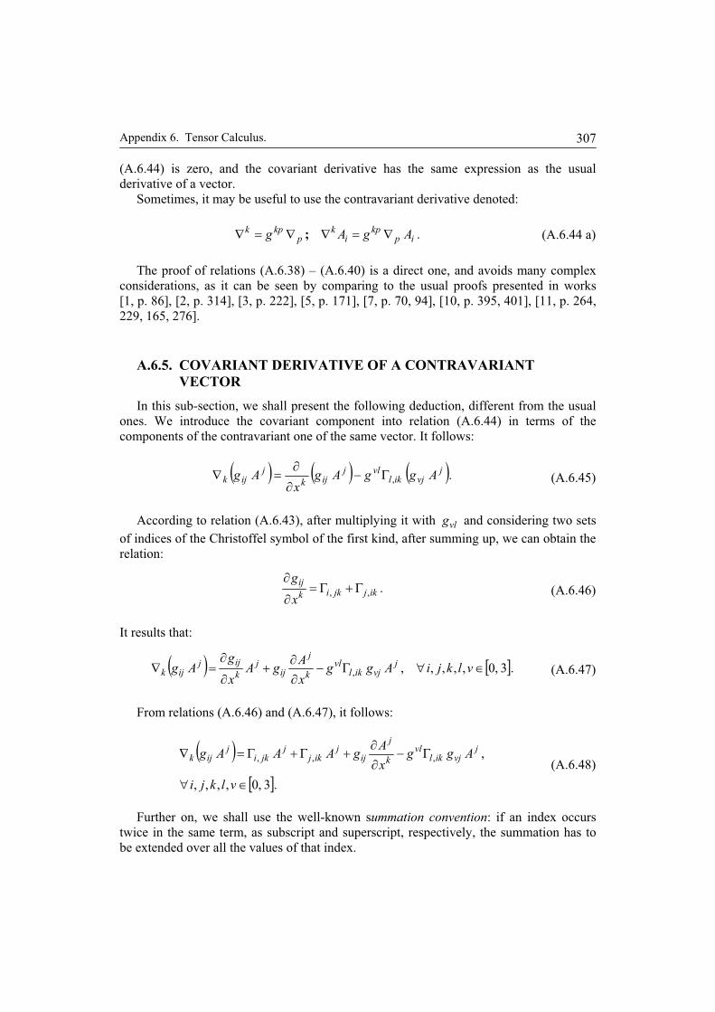
Appendix 6. Tensor Calculus. 307
(A.6.44) is zero, and the covariant derivative has the same expression as the usual derivative of a vector.
Sometimes, it may be useful to use the contravariant derivative denoted:
ipkp
ik
pkpk AgAg ; . (A.6.44 a)
The proof of relations (A.6.38) – (A.6.40) is a direct one, and avoids many complex considerations, as it can be seen by comparing to the usual proofs presented in works [1, p. 86], [2, p. 314], [3, p. 222], [5, p. 171], [7, p. 70, 94], [10, p. 395, 401], [11, p. 264, 229, 165, 276].
A.6.5. COVARIANT DERIVATIVE OF A CONTRAVARIANTVECTOR
In this sub-section, we shall present the following deduction, different from the usual ones. We introduce the covariant component into relation (A.6.44) in terms of the components of the contravariant one of the same vector. It follows:
.,j
vjiklvlj
ijk
jijk AggAg
xAg (A.6.45)
According to relation (A.6.43), after multiplying it with vlg and considering two sets of indices of the Christoffel symbol of the first kind, after summing up, we can obtain the relation:
.,, ikjjkik
ij
x
g(A.6.46)
It results that:
.3,0,,,,,, vlkjiAggx
AgA
x
gAg j
vjiklvl
k
j
ijj
k
ijjijk (A.6.47)
From relations (A.6.46) and (A.6.47), it follows:
.3,0,,,,
,,,,
vlkji
Aggx
AgAAAg j
vjiklvl
k
j
ijj
ikjj
jkij
ijk(A.6.48)
Further on, we shall use the well-known summation convention: if an index occurs twice in the same term, as subscript and superscript, respectively, the summation has to be extended over all the values of that index.

General Theory of the Electromagnetic Field 308
In the last term of relation (A.6.48), according to the summation convention, for any
value of the index v, the product vjvl gg , is zero, except the case lj , in which it is
equal to unity. This results by using the expression DDg jiij / , where D is the
determinant having the elements ijg , and jiD is the cofactor (minor) of the element jig ,
or directly, by using formula (A.6.30). But then, since jl , the sum of the second term and of the last term of the right-hand side vanishes. Therefore:
,3,0,,,,, lkjix
AgAAg
k
j
ijl
lkij
ijk (A.6.49)
where we have replaced j by l, both taking successively the same values.
Multiplying both sides of relation (A.6.49) by irg , where r represents an integer fixed value, comprised between zero and 3 inclusive, we get:
.3,0,,,,, lkjix
AggAgAgg
k
j
ijirl
lkiirj
ijkir
(A.6.50)
Considering the summation convention, and making the same remark as before, which have led to relation (A.6.49), we obtain:
.3,0,,,,, rlkjix
AAAgg
k
rlr
lkj
ijkir
(A.6.51)
Finally, we denote:
,3,0,,,,, rlkjiAx
AAggA lr
lkk
rj
ijkirr
k (A.6.52)
which is called the covariant derivative of a contravariant vector.
A.6.5.1. Geodesic Lines
Let us replace, in relation (A.6.52), the vector rA by s
xr
d
d, where sxr and ds
denote the co-ordinates of each point and the element of the arc s of a curve, respectively,
equate the relation to zero, and multiply the equation with s
xk
d
d. We shall obtain the
equation of a geodesic curve also called geodesic line. Accordingly, we consider equation (A.6.52) in the form:
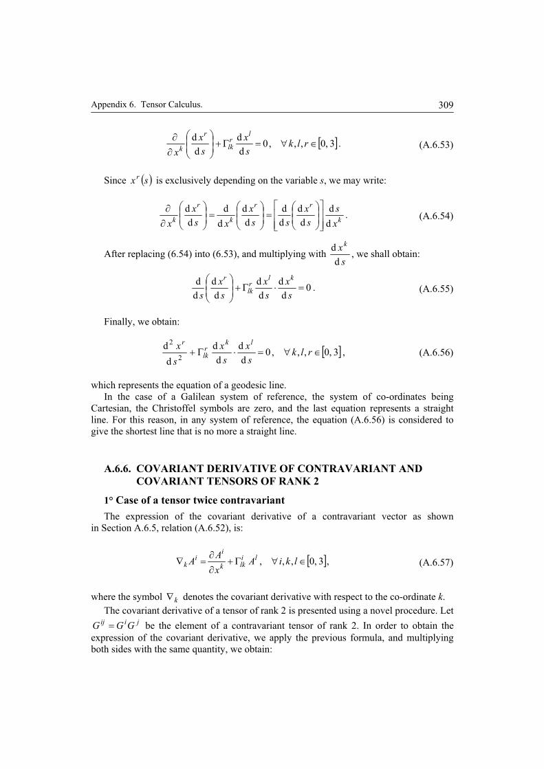
Appendix 6. Tensor Calculus. 309
3,0,,,0d
d
d
drlk
s
x
s
x
x
lrlk
r
k. (A.6.53)
Since sxr is exclusively depending on the variable s, we may write:
k
rr
k
r
k x
s
s
x
ss
x
xs
x
x d
d
d
d
d
d
d
d
d
d
d
d. (A.6.54)
After replacing (6.54) into (6.53), and multiplying with s
xk
d
d, we shall obtain:
0d
d
d
d
d
d
d
d
s
x
s
x
s
x
s
klrlk
r
. (A.6.55)
Finally, we obtain:
3,0,,,0d
d
d
d
d
d2
2
rlks
x
s
x
s
x lkrlk
r
, (A.6.56)
which represents the equation of a geodesic line. In the case of a Galilean system of reference, the system of co-ordinates being Cartesian, the Christoffel symbols are zero, and the last equation represents a straight line. For this reason, in any system of reference, the equation (A.6.56) is considered to give the shortest line that is no more a straight line.
A.6.6. COVARIANT DERIVATIVE OF CONTRAVARIANT AND COVARIANT TENSORS OF RANK 2
1° Case of a tensor twice contravariant
The expression of the covariant derivative of a contravariant vector as shown in Section A.6.5, relation (A.6.52), is:
,3,0,,, lkiAx
AA li
lkk
ii
k (A.6.57)
where the symbol k denotes the covariant derivative with respect to the co-ordinate k. The covariant derivative of a tensor of rank 2 is presented using a novel procedure. Let
jiij GGG be the element of a contravariant tensor of rank 2. In order to obtain the expression of the covariant derivative, we apply the previous formula, and multiplying both sides with the same quantity, we obtain:

General Theory of the Electromagnetic Field 310
.3,0,,,, lkjiGGGGGx
G jlilk
jik
j
k
i
(A.6.58)
Similarly, using the same formula, we shall obtain:
.3,0,,,, lkjiGGGGx
GG lj
lkij
ki
k
ji
(A.6.59)
Finally, by summing up, we may write:
,iljlk
ljilkk
ijij
kj
kiji
k GGx
GGGGGG (A.6.60)
which is the expression of the covariant derivative of the contravariant tensor ijG .
2° Case of a tensor twice covariant The expression of the covariant derivative of a covariant vector as shown in Section A.6.4, relation (A.6.44), is:
., viklvl
ki
ik Agx
AA (A.6.61)
Let jiij GGG be the element of a covariant tensor of rank 2. Proceeding like above,
we shall obtain:
.illjklj
likk
ijijkjktjik GG
x
GGGGGG (A.6.62)
3° Case of a mixed tensor once covariant and once contravariant Let j
ij
i GGG be the element of the considered tensor. Performing calculations like
above, we shall obtain:
,li
jlk
jl
likk
jij
ikj
kij
ik GGx
GGGGGG (A.6.63)
and:
.li
jlk
jl
likk
jij
ik GGx
GG (A.6.64)
4° Case of the fundamental covariant tensor Let ijg be the element (component) of the considered tensor. Performing calculations like
above, we shall obtain:

Appendix 6. Tensor Calculus. 311
,illjklj
likk
ijijk gg
x
gg (A.6.65)
and according to (6.43):
., ,, jkvlvl
jkikvlvl
ik gg (A.6.65 a)
By replacing the factors lik and l
jk into (6.65), we shall obtain:
.3,0,,,,,, vkjiggx
gg v
ijkvvjikvk
ijijk (A.6.66)
Taking into account (A.6.30), we shall obtain:
.3,0,,,,, kjix
gg jkiikjk
ijijk (A.6.67)
According to relations (A.6.46), (A.6.67) and also (A.6.32), it results that:
.0;0 ijkijk gg (A.6.68)
A.6.7. THE DIVERGENCE OF TENSORS OF RANKS 1 AND 2
We shall start, in this Section, from the covariant derivative of a vector. The most general case will be examined in the next Chapter. The divergence of a vector in a Cartesian system of co-ordinates is:
.3,0;, iikx
AA
k
ii
k (A.6.69)
Indeed, relation (A.6.57) holds for any value of any value of indices i and k, among which, for instance 2i , 2k , and so on, and summing up side by side, we get the result. Therefore, the expression of the divergence of a vector in any system of co-ordinates is obtained starting from the relation (A.6.57), contracted on indices i, k:
,lilii
ii
i Ax
AA (A.6.70)

General Theory of the Electromagnetic Field
312
in which, in the case of a Cartesian system of co-ordinates the second term of the right-hand side vanishes. According to relation (A.6.43), where we introduce the indices for the present case as follows: ;;; livliv === taking into account the contraction on indices
,, ki we shall obtain:
.,21
, kigxg
xg
xg
g ivvlk
lkv
klv
lkvivi
lk =⎟⎟⎠
⎞⎜⎜⎝
⎛
∂
∂−
∂
∂+
∂
∂=Γ=Γ (A.6.71)
We now want to calculate:
., kigxg
gxg iv
vlkiv
klv =
∂
∂−
∂
∂ (A.6.72)
Since the indices ik = and v can take all values from zero to 3, we can replace k by v, and v by k in the first term, and the previous expression becomes:
,kvvlkvk
vlk g
xg
gxg
∂
∂−
∂
∂ (A.6.73)
the value of which is zero. Therefore:
.,21
, kixg
gg lkvkv
lkvivi
lk =∂
∂=Γ=Γ (A.6.74)
Let us use the following symbols: D – the determinant formed by the elements ijg ; ijD – the cofactor of the element ijg ; g – the value of D. Since the elements ijg are
those of the inverse matrix corresponding to the determinant, we express those elements by the corresponding formulae. Taking into account the expression of the derivative of a determinant, and that of the symmetry property of determinant D, we obtain:
[ ],3,0,;;; ∈∀∂∂
=∂∂
== vkDxgD
xDgD
DDg kv
lkv
lkv
kv
kvkv (A.6.75 a)
and also:
[ ]3,0,;,,1∈∀==
∂∂⋅=
∂∂⋅=
∂∂ vkDgki
xD
Dxg
DD
xgg ll
kvkv
lkvkv . (A.6.75 b)
Therefore, from relations (A.6.74) and (A.6.75 b), it follows:

Appendix 6. Tensor Calculus.
313
,,121
21
, kixg
gxg
gg llkvkv
lkvivi
lk =∂
∂⋅⋅=
∂
∂=Γ=Γ (A.6.76)
where, for simplicity, we have replaced D by g. From relations (A.6.70) and (A.6.76), it follows:
.,121
, kiAxg
gxAAg
xAA l
li
il
lkviv
k
ii
k =∂
∂⋅⋅+
∂
∂=Γ+
∂
∂=∇ (A.6.77)
Taking into account that in relation (A.6.73), the indices ki = and l take all values from zero to 3, we replace l by ki = in the last term. It follows:
.121 i
ii
ii
i Axg
gxAA
∂
∂⋅⋅+
∂
∂=∇ (A.6.78)
The last relation may be transformed using (A.6.79 a), in the final form (A.6.79 a, b):
( ) ;121
xAgA
gAg
x ∂∂
+⋅=∂∂
( ),1Div ii
ii
i Agxg
AA ±∂∂
⋅±
=∇=
(A.6.79 a, b)
where the plus and minus signs from denominator and numerator correspond to each other, the sign minus being taken if g is negative. The symbol Div, instead of div, has been used in order to emphasize the general system of reference. The expression of the divergence of a tensor of rank 2 may be written similarly, starting from formula (A.6.60), contracted on indices j and k:
[ ] .,3,0,, jkjiGGxGG ilj
lklji
lkk
ijij
j =∈∀Γ+Γ+∂∂
=∇ (A.6.80)
In the case in which the tensor ljG is antisymmetric in the superscript indices j and l, whereas the factor i
lkΓ is always symmetric in the subscript indices l and jk = , the first term of the right-hand side of (A.6.80) vanishes. It results that:
[ ] .3,0,,, ∈∀Γ+∂∂
=∇ ljiGxGG ilj
ljj
ijij
j (A.6.81)
Similarly as for relations (A.6.70) – (A.6.78), we get:
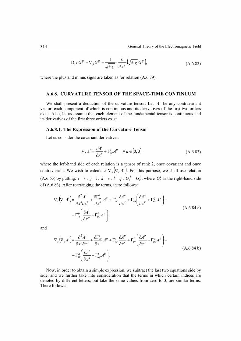
General Theory of the Electromagnetic Field 314
,1
Div ij
j
ijj
ij Ggxg
GG (A.6.82)
where the plus and minus signs are taken as for relation (A.6.79).
A.6.8. CURVATURE TENSOR OF THE SPACE-TIME CONTINUUM
We shall present a deduction of the curvature tensor. Let iA be any contravariant vector, each component of which is continuous and its derivatives of the first two orders exist. Also, let us assume that each element of the fundamental tensor is continuous and its derivatives of the first three orders exist.
A.6.8.1. The Expression of the Curvature Tensor
Let us consider the covariant derivatives:
,3,0uAx
AA ui
urr
ii
r (A.6.83)
where the left-hand side of each relation is a tensor of rank 2, once covariant and once
contravariant. We wish to calculate irs A . For this purpose, we shall use relation
(A.6.63) by putting: ri , ij , sk , ql , ir
ji GG , where i
rG is the right-hand side
of (A.6.83). After rearranging the terms, there follows:
,
2
uiuqq
iqrs
uqurr
qiqss
uiur
u
s
iur
rs
ii
rs
Ax
A
Ax
A
x
AA
xxx
AA
(A.6.84 a)
and
.
2
uiuqq
iqsr
uquss
qiqrr
uius
u
r
ius
sr
ii
sr
Ax
A
Ax
A
x
AA
xxx
AA
(A.6.84 b)
Now, in order to obtain a simple expression, we subtract the last two equations side by side, and we further take into consideration that the terms in which certain indices are denoted by different letters, but take the same values from zero to 3, are similar terms. There follows:

Appendix 6. Tensor Calculus. 315
.uqus
iqr
qur
iqs
u
r
ius
s
iuri
srrs AAxx
A (A.6.85)
The expression (A.6.85) may be written:
.uirsu
isrrs ARA (A.6.86)
The factor irsuR of expression (A.6.86), is also called the Riemann curvature tensor, in
which we have separated, by parentheses, two terms:
qus
iqr
qur
iqsr
ius
s
iuri
rsuxx
R , (A.6.87)
which is a tensor of rank 4, three times covariant and once contravariant. By contracting with respect to indices i and r, we obtain:
qus
rqr
qur
rqsr
rus
s
rur
suxx
R , (A.6.88)
which is a covariant tensor of rank 2, also called Ricci tensor.
A.6.8.2. Geodesic Co-ordinates
The geodesic co-ordinates are those in which Christoffel symbols are zero, but their derivatives with respect to co-ordinates may be different from zero. Therefore, the covariant derivative of expression (A.6.87) concerns only the first parenthesis and is:
rk
ius
sk
iuri
rsukxxxx
R22
. (A.6.89)
Using relation (A.6.89), and changing the indices, there follows:
0iskur
ikrus
irsuk RRR , (A.6.90)
which is the Bianchi identity.Besides the relations above, the geodesic co-ordinate system has been used in certain
applications [3, p. 232]. We recall, more detailed than usually, that a geodesic reference system, generally, can be considered in a small space around any chosen point. The elements (components) of the fundamental tensor are assumed to be functions of point, the first derivatives of which have, at the chosen point, the value zero, but their derivatives of higher orders may exist. If a tensor is zero at that point, it will keep the value zero, at that point, in any other system of reference.
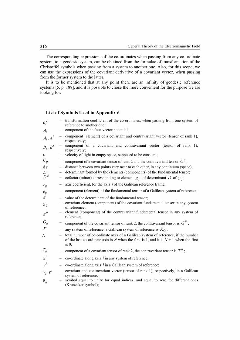
General Theory of the Electromagnetic Field 316
The corresponding expressions of the co-ordinates when passing from any co-ordinate system, to a geodesic system, can be obtained from the formulae of transformation of the Christoffel symbols when passing from a system to another one. Also, for this scope, we can use the expressions of the covariant derivative of a covariant vector, when passing from the former system to the latter.
It is to be mentioned that at any point there are an infinity of geodesic reference systems [5, p. 188], and it is possible to chose the more convenient for the purpose we are looking for.
List of Symbols Used in Appendix 6
jia – transformation coefficient of the co-ordinates, when passing from one system of
reference to another one;
iA – component of the four-vector potential;
ii AA , – component (element) of a covariant and contravariant vector (tensor of rank 1),
respectively;i
i BB , – component of a covariant and contravariant vector (tensor of rank 1), respectively;
c – velocity of light in empty space, supposed to be constant;
ijC – component of a covariant tensor of rank 2 and the contravariant tensor ijC ;
sd – distance between two points very near to each other, in any continuum (space); D – determinant formed by the elements (components) of the fundamental tensor;
jiD – cofactor (minor) corresponding to element jig of determinant D of ijg ;
iie – axis coefficient, for the axis i of the Galilean reference frame;
ije – component (element) of the fundamental tensor of a Galilean system of reference;
g – value of the determinant of the fundamental tensor;
ijg – covariant element (component) of the covariant fundamental tensor in any system of reference;
ijg – element (component) of the contravariant fundamental tensor in any system of reference;
ijG – component of the covariant tensor of rank 2, the contravariant tensor is ijG ;
K – any system of reference, a Galilean system of reference is GK ;
N – total number of co-ordinate axes of a Galilean system of reference, if the number of the last co-ordinate axis is N when the first is 1, and it is N + 1 when the first is 0;
ijT – component of a covariant tensor of rank 2, the contravariant tensor is ijT ;ix – co-ordinate along axis i in any system of reference; iy – co-ordinate along axis i in a Galilean system of reference;
ii YY , – covariant and contravariant vector (tensor of rank 1), respectively, in a Galilean
system of reference;
ij– symbol equal to unity for equal indices, and equal to zero for different ones
(Kronecker symbol);
Appendix 6. Tensor Calculus. 317
,l ik– Christoffel symbol of the first kind;
vik
– Christoffel symbol of the second kind;
k– covariant derivative with respect to co-ordinate k;
k – contravariant derivative with respect to co-ordinate k.
REFERENCES
1. EINSTEIN, A.: The Meaning of Relativity. Princeton University Press, Princeton, New Jersey, 1955. Teoria relativit ii. Editura Tehnic , Bucure ti, 1957.
2. LANDAU, L., LIFCHITZ, E.: Théorie des champs. Éditions Mir, Moscou, 1970. 3. FOCK, V.A.: The Theorie of Space, Time and Gravitation, (translated by N. Kemmer).
Pergamon Press, London, 1959. Teoria spa iului timpului i gravita iei. Ed. Academiei Române, Bucure ti, 1962.
4. ARZELIÈS, H.: Électricité. Le point de vue macroscopique et relativiste. Gauthier-Villars, Éditeur, Paris, 1963.
5. PATHRIA, R.K.: The theory of relativity. Second edition, Pergamon Press, Oxford, New York, Toronto, Hindustan Publishing Corporation (India), Delhi, 1974.
6. FOURNET, G.: Électromagnétisme à partir des équations locales. Masson et C-ie, Éditeurs, Paris, 1985.
7. LUDVIGSEN, M.: La relativité générale. Une approche géométrique. Dunod, Paris, 2000.
8. NICOLAIDE, A.: Considerations on the energy-momentum tensor in the special and general
theory of relativity. Rev. Roum. Sci. Techn. – Électrotechn. et Énerg., 51, 4, pp. 405-417 (2006).
9. NICOLAIDE, A.: Considerations on the covariant form of the equations of the
electromagnetic field in polarized media. Rev. Roum. Sci. Techn. – Électrotechn. et Énerg., 53, 1, pp. 11-22 (2008).
10. KOCHIN, N.E.: Vector calculus and introduction to tensor calculus. Seventh edition. Publishing House of the Academy of Sciences, Moscow, 1951. KOCIN, N.E.: Calculul vectorial i introducere în calculul tensorial. Edit. Tehnic , Bucure ti, 1954.
11. DOUBROVINE, B.A., NOVIKOV, S.P., FOMENKO, A.T.: Géométrie contemporaine. Méthodes
et applications. Première partie. Éditions Mir, Moscou, 1985. 12. Prove that 4 vector potential is really a vector.
16 messages, 6 authors. www.physicsforums.com/archive/index.php/t-232693.html - 83 k; 27th Oct., 2008.
13. NICOLAIDE, A.: Deriving the formula of the Sagnac effect by using the general theory of
relativity. Rev. Roum. Sci. Techn. – Électrotechn. et Énerg., 51, 1, pp. 3-11 (2006). 14. BRILLOUIN, L.: Cours de Physique théorique. Les tenseurs en mécanique et en élasticité.
Masson et C-ie, Éditeurs, Paris, 1946.

General Theory of the Electromagnetic Field 318
APPENDIX 7
THE VARIOUS DIVERGENCE TYPES OF A TENSOR AND OF THE CURVATURE TENSOR IN THE GENERAL THEORY OF RELATIVITY
In Appendix 6, we have presented the calculation of the divergence of various types of tensors that often occurs. Further on, we shall examine the general expressions of the differential operator divergence. The bibliographic mentions [1]-[12], specific for this Appendix, are at the end of this Appendix.
A.7.1. DIVERGENCE OF A TENSOR
The calculation of the divergence of a tensor occurs in many problems of Physical Mathematics. We consider that the notion of divergence of a tensor has not been enough defined and analysed in the usual literature. We shall try to establish a consistent definition of a tensor including the calculation procedure, and to apply it to the calculation of the divergence of the curvature tensor of the four-dimensional continuum space-time.
Several studies on the divergence of tensors have been carried out for a long time, [1]-[10]. In paper [10], a deep study on the differential operations on tensors has been performed without using the tensor calculus, but instead the general method concerning the differential quadratic forms, from the classical mathematical analysis, has been utilized. The methods used in the other papers will be examined further on.
In order to facilitate the understanding, and have a uniform system of symbols, the paper includes three Sub-sections: the first one containing several tensor formulae frequently used in the paper; the second one presenting a relatively simple deduction of the Riemann curvature; and the third one containing a very short deduction of the Bianchi identity.
A.7.2. THE DIVERGENCE OF COVARIANT AND CONTRAVARIANT TENSORS
The calculation of the divergence of a tensor, as known, is based on the calculation of the derivative of that tensor. The divergence of a vector in a Cartesian system of co-ordinates is:
[ ].3,0;, ∈=∀∂∂
=∇ iikxAA k
ii
k (A.7.1)

General Theory of the Electromagnetic Field
320
We recall the symbols of the covariant and contravariant derivatives, namely k∇ and k∇ , respectively. Correspondingly, we may use the denominations of covariant and
contravariant divergence, respectively. The expression of the covariant derivative of a contravariant tensor of rank 1, i.e. a
contravariant vector, is:
[ ],3,0,,, ∈∀Γ+∂∂
=∇ kliAxAA li
lkk
ii
k (A.7.2)
where lkv,Γ , and lkvivi
lk g ,Γ=Γ are the Christoffel symbols of the first and second kind respectively. The expression of the divergence of a vector in any system of co-ordinates is obtained starting from the relation (A.7.2), contracted in indices ki, :
[ ],3.0,, ∈∀Γ+∂∂
=∇ liAxAA li
lii
ii
i (A.7.3)
and represents a tensor of rank zero, i.e., a scalar. Relation (A.7.3) may also be written:
( ) [ ],3,0,1Div ∈∀±∂∂
⋅±
=∇= iAgxg
AA ii
ii
i (A.7.3 a)
where g represents the value of the determinant of the fundamental tensor, and the plus and minus signs from denominator and numerator correspond to each other, the sign minus being taken if g is negative. The symbol Div, instead of div, has been used in order to emphasize the general system of reference.
The covariant derivative of a covariant tensor of rank 1, i.e., a covariant vector, is given by the following relation, and its divergence results by contracting the expression in indices i and k:
.,, ikAgxAA vikl
vlki
ik =Γ−∂∂
=∇ (A.7.4)
The contravariant derivative of the same tensor is given by the following relation, and its divergence results by contracting the expression in indices i and k:
.,, ikAgxAgAgA vpil
vlpipk
ippk
ik =⎟⎟
⎠
⎞⎜⎜⎝
⎛Γ−
∂∂
=∇=∇ (A.7.5)
The expression of the divergence of a contravariant tensor of rank 2 may be written similarly, starting from the formula of the covariant derivative of a twice contravariant tensor ijG , contracted in indices j and k:
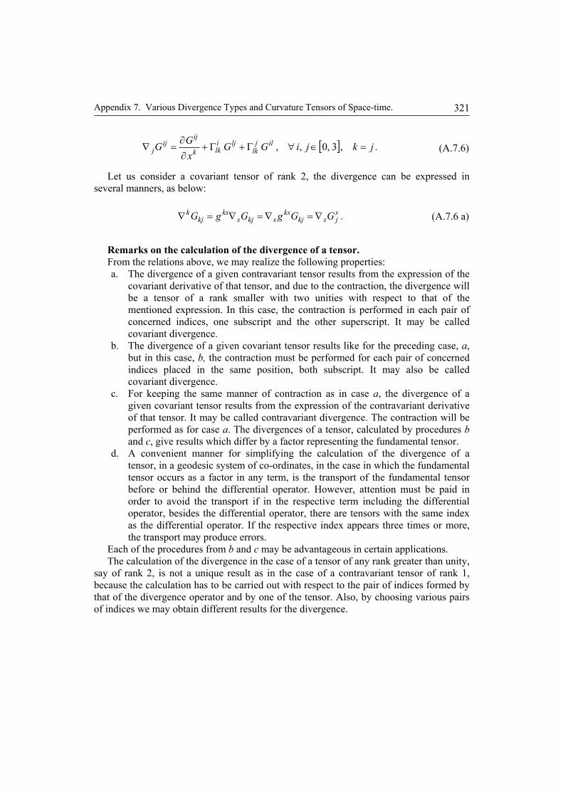
Appendix 7. Various Divergence Types and Curvature Tensors of Space-time.
321
[ ] .,3,0,, jkjiGGxGG ilj
lklji
lkk
ijij
j =∈∀Γ+Γ+∂∂
=∇ (A.7.6)
Let us consider a covariant tensor of rank 2, the divergence can be expressed in several manners, as below:
sjskj
ksskjs
kskj
k GGgGgG ∇=∇=∇=∇ . (A.7.6 a)
Remarks on the calculation of the divergence of a tensor. From the relations above, we may realize the following properties: a. The divergence of a given contravariant tensor results from the expression of the
covariant derivative of that tensor, and due to the contraction, the divergence will be a tensor of a rank smaller with two unities with respect to that of the mentioned expression. In this case, the contraction is performed in each pair of concerned indices, one subscript and the other superscript. It may be called covariant divergence.
b. The divergence of a given covariant tensor results like for the preceding case, a, but in this case, b, the contraction must be performed for each pair of concerned indices placed in the same position, both subscript. It may also be called covariant divergence.
c. For keeping the same manner of contraction as in case a, the divergence of a given covariant tensor results from the expression of the contravariant derivative of that tensor. It may be called contravariant divergence. The contraction will be performed as for case a. The divergences of a tensor, calculated by procedures b and c, give results which differ by a factor representing the fundamental tensor.
d. A convenient manner for simplifying the calculation of the divergence of a tensor, in a geodesic system of co-ordinates, in the case in which the fundamental tensor occurs as a factor in any term, is the transport of the fundamental tensor before or behind the differential operator. However, attention must be paid in order to avoid the transport if in the respective term including the differential operator, besides the differential operator, there are tensors with the same index as the differential operator. If the respective index appears three times or more, the transport may produce errors.
Each of the procedures from b and c may be advantageous in certain applications. The calculation of the divergence in the case of a tensor of any rank greater than unity,
say of rank 2, is not a unique result as in the case of a contravariant tensor of rank 1, because the calculation has to be carried out with respect to the pair of indices formed by that of the divergence operator and by one of the tensor. Also, by choosing various pairs of indices we may obtain different results for the divergence.

General Theory of the Electromagnetic Field
322
A.7.3. APPLICATION TO THE CASE OF THE RIEMANN
CURVATURE TENSOR AND EINSTEIN TENSOR
The equations of the classical General Theory of Relativity contain the Einstein tensor developed starting from the Riemann tensor of the four-dimensional continuum space-time.
In the work [1], Einstein has directly given the tensor considered to satisfy the three required conditions the value zero of the divergence included. Let us consider the Einstein tensor:
,RgaR ijij + (A.7.7)
where Rij is the Riemann tensor of rank 2, also called Ricci tensor, R is given by the relation:
iiij
ij RRgR == , (A.7.8)
and a is a constant. Also, there is added that for the third condition to be satisfied, the
constant a should be equal to 21−
. The same expression is given in many works, among
which [3, p. 248], [4, p. 201], [5, p. 99].
7.4. REMARKS CONCERNING THE CALCULATION OF EXPRESSIONS INVOLVING THE RIEMANN TENSOR
In order to clarify the calculation of the tensor divergence, avoiding certain errors, we shall consider an example concerning the mixed Riemann tensor of rank four and its transformation into a covariant tensor of the same rank. Although well known, we shall remake a simple deduction in order to emphasize a very important property accepted but never explicitly mentioned in the known works. Let us consider the mixed expression of the tensor below and transform it into a covariant one. For the next calculations, we shall take into account relations (A.6.28) – (A.6.32). Therefore, we shall start with (A.6.87):
..... qus
iqr
qur
iqsr
ius
s
iuri
rsu xxR ΓΓ−ΓΓ+
∂
Γ∂−
∂
Γ∂= (A.7.9)
Let us look to express into a covariant form the tensor of the right-hand side of the formula below:
.....irsuiprsup RgR = (A.7.10)
There follows:
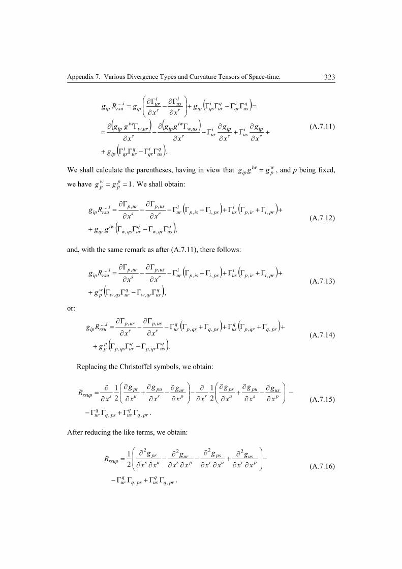
Appendix 7. Various Divergence Types and Curvature Tensors of Space-time.
323
( )( ) ( )
( ).
,,
....
qus
iqr
qur
iqsip
ripi
ussipi
urrusw
iwip
surw
iwip
qus
iqr
qur
iqsipr
ius
s
iur
ipi
rsuip
g
x
g
x
g
x
gg
x
gg
gxx
gRg
ΓΓ−ΓΓ+
+∂
∂Γ+
∂
∂Γ−
∂
Γ∂−
∂
Γ∂=
=ΓΓ−ΓΓ+⎟⎟⎠
⎞⎜⎜⎝
⎛
∂Γ∂
−∂Γ∂
=
(A.7.11)
We shall calculate the parentheses, having in view that wp
iwip ggg = , and p being fixed,
we have 1== pp
wp gg . We shall obtain:
( ) ( )
( ),,,
,,,,,,....
qusqrw
qurqsw
iwip
priirpiuspsiisp
iurr
uspsurpi
rsuip
gg
xxRg
ΓΓ−ΓΓ+
+Γ+ΓΓ+Γ+ΓΓ−∂
Γ∂−
∂
Γ∂=
(A.7.12)
and, with the same remark as after (A.7.11), there follows:
( ) ( )
( ),,,
,,,,,,....
qusqrw
qurqsw
wp
priirpiuspsiisp
iurr
uspsurpi
rsuip
g
xxRg
ΓΓ−ΓΓ+
+Γ+ΓΓ+Γ+ΓΓ−∂
Γ∂−
∂
Γ∂=
(A.7.13)
or:
( ) ( )
( ).,,
,,,,,,....
qusqrp
qurqsp
pp
prqqrpquspsqqsp
qurr
uspsurpi
rsuip
g
xxRg
ΓΓ−ΓΓ+
+Γ+ΓΓ+Γ+ΓΓ−∂
Γ∂−
∂
Γ∂=
(A.7.14)
Replacing the Christoffel symbols, we obtain:
.
21
21
,, prqquspsq
qur
pus
spu
ups
rpur
rpu
upr
srsup xg
xg
xg
xxg
xg
xg
xR
ΓΓ+ΓΓ−
−⎟⎟⎠
⎞⎜⎜⎝
⎛
∂∂
−∂
∂+
∂
∂
∂∂
−⎟⎟⎠
⎞⎜⎜⎝
⎛
∂∂
−∂
∂+
∂
∂
∂∂
= (A.7.15)
After reducing the like terms, we obtain:
.
21
,,
2222
prqquspsq
qur
prus
urps
psur
uspr
rsup xxg
xxg
xxg
xxg
R
ΓΓ+ΓΓ−
−⎟⎟
⎠
⎞
⎜⎜
⎝
⎛
∂∂∂
+∂∂
∂−
∂∂∂
−∂∂
∂=
(A.7.16)

General Theory of the Electromagnetic Field
324
The relation (A.7.16) contains the components of the fundamental tensor ijg in the system of reference K . These quantities may be obtained by using formula (A.6.20), starting from a quasi-Euclidean system of reference GK .
Some general relations, deduced from (A.6.3 a, b) extended for tensors of rank 2, and (A.6.41), could facilitate the understanding:
[ ] [ ];,0,,3,0,
;1;
;1;
0,
0,
0
0
Nbaji
yx
yxg
eyx
yxge
xy
xye
gxy
xyeg
b
j
a
i
ij
N
ba
abb
j
a
i
ij
N
baab
j
a
i
a
aa
Na
a
ijj
a
i
a
aa
N
aij
∈∈∀
∂∂⋅
∂∂
=∂∂⋅
∂∂
=
∂∂⋅
∂∂
=∂∂⋅
∂∂
=
∑∑
∑∑
=
=
=
=
=
(A.7.16 a-d)
where we have deduced the formulae of the contravariant components from the inverse matrix of the covariant components, having advantages relatively to those of literature.
According to formula (A.7.16 a) above, the passage from the quantities ay to the components ijg is always possible, obtaining say 10 components in terms of say ( ) 41 ≥+N other quantities. Conversely, for passing from the components ijg to
components abe we have to resort to the formula (A.7.16 c), say 10 equations. But in this case, supplementary conditions, namely baeab ≠∀= ,0 hence other 6 other equations, must be fulfilled (although previously not imposed) the respective reference frame GK being quasi-Euclidean. Finally, we shall have 4 unknowns and 16 equations. There follows that the number of equations to be fulfilled is greater than the number of unknowns, the solution being, in general, impossible. It follows that the correspondence between GK and K , is not biunivocal, the obtained expression of the curvature being valid only for the reference frame K .
7.5. CALCULATION OF THE DIVERGENCE GIVEN BY THE AUTHORS USING THE BIANCHI IDENTITY
The majority of the known authors have used the Bianchi identity for this purpose [1]-[5], [8]. In this case, they start from a tensor of rank four, in order to establish the property of a tensor of rank 2, what seems to be an indirect and more complicated way. Further, a set of transformations bring the expression from a vector of rank four to a vector of rank 2, namely a mixed vector.
The proofs, aiming the calculation of the divergence of the curvature tensor are based on Bianchi identity and on the usage of the geodesic co-ordinates, like in works [1]-[5].

Appendix 7. Various Divergence Types and Curvature Tensors of Space-time.
325
According to relation (A.6.90) and the inversion of indices r and s , in the last two terms, the following identity may be written:
.0=∇−∇−∇ iksur
irkus
irsuk RRR (A.7.17)
By putting i = r, and contracting with respect to index i, there follows:
.0=∇−∇−∇ iksuikussuk RRR (A.7.18)
Multiplying the last relation by sug , and taking into account relation (A.6.32), one will obtain:
,0=∇−∇−∇ iki
sks
ssk RRR (A.7.19)
and replacing index s by i in the second term of the left-hand side of relation (A.7.19), both taking all values from zero to 3, one obtains:
.02 =∇+∇− iki
ssk RR (A.7.20)
From here on, we shall modify the known procedure [4, p. 201], avoiding the Kronecker symbol. Starting from relation (A.7.20) and changing the first index of the first term, we get:
,02 =∇+∇− iki
ss
iki RRg (A.7.21)
and taking into account (A.7.8), we obtain
,021
=⎟⎠⎞
⎜⎝⎛ −∇ RgR i
kiki (A.7.22)
where the term within parentheses corresponds to that of Einstein tensor, but in a mixed form.
7.6. THE PROPOSED NEW PROOF
Unlike to the other methods we shall consider the tensor we are looking for as not known. Let us start from the general formula of the Riemann curvature in geodesic co-ordinates expressed as a tensor of rank 2:
[ ],3,0, ∈∀⎟⎟⎠
⎞⎜⎜⎝
⎛
∂Γ∂
−∂Γ∂
= rxx
R r
rus
s
rur
su (A.7.23)

General Theory of the Electromagnetic Field
326
and s and u are fixed values chosen from the set [ ]3,0 . Then, from formula (A.7.23), also using geodesic co-ordinates, we get:
[ ] ,3,0∈∀
∂Γ∂
⋅∂∂
−∂Γ∂
⋅∂∂
=⎟⎟⎠
⎞⎜⎜⎝
⎛
∂Γ∂
−∂Γ∂
∂∂
=⎟⎟⎠
⎞⎜⎜⎝
⎛
∂Γ∂
−∂Γ∂
∇=∇
rxxxxxxxxx
R k
rus
rk
rur
sr
rus
s
rur
kr
rus
s
rur
ksuk (A.7.24)
and k, s, u are fixed values chosen from the set [ ]3,0 . Therefore, according to formula (A.7.23) or (A.7.24), by adding and subtracting the same term, we can write:
[ ],3,0
,
∈∀
⎟⎟⎠
⎞⎜⎜⎝
⎛
∂Γ∂
−∂Γ∂
∂∂
+⎟⎟⎠
⎞⎜⎜⎝
⎛
∂Γ∂
−∂Γ∂
∂∂
=∇
rxxxxxx
R k
rus
s
ruk
rr
ruk
k
rur
ssuk (A.7.25)
and k, s, u are fixed values, like in the preceding relation. Consequently:
[ ]3,0, ∈∀⎟⎟⎠
⎞⎜⎜⎝
⎛
∂Γ∂
−∂Γ∂
∂∂
+⎟⎟⎠
⎞⎜⎜⎝
⎛
∂Γ∂
−∂Γ∂
∂∂
=∇ rxxxxxx
R k
wus
s
wuk
wr
ruk
k
rur
ssuk (A.7.26)
or, with the symbols similar to those of (A.7.24), we have:
[ ].3,0, ∈∀∇+∇=∇ wRRR wksuwkussuk (A.7.27)
After rearranging the terms, we obtain:
[ ].3,0,0 ∈∀=∇−∇−∇ wRRR wksuwkussuk (A.7.28)
By multiplying both sides with sug , it follows:
[ ].3,0,0 ∈∀=∇+∇+∇− wRRR wkw
sks
ssk (A.7.29)
Therefore:
.02 =∇+∇− sks
ssk RR (A.7.30)
Let us use the contravariant derivative:
.02 =∇+∇− sksp
psskp
p RgRg (A.7.31)
Taking into account relation (A.7.8), relation (A.7.31) yields:

Appendix 7. Various Divergence Types and Curvature Tensors of Space-time.
327
[ ].3,0,021
∈∀=⎟⎠⎞
⎜⎝⎛ −∇ pRgR kpkp
p (A.7.32)
Therefore, we have just deduced the divergence of the Einstein tensor, by a so-called inductive way, without resorting to the Bianchi identity. Due to its form, relation (A.7.32) may be called contravariant divergence.
RFERENCES
1. EINSTEIN, A.:The Meaning of Relativity. Princeton University Press, Princeton, New Jersey, 1955. Teoria relativităţii. Editura Tehnică, Bucureşti, 1957.
2. LANDAU, L., LIFCHITZ, E.: Théorie des champs. Éditions Mir, Moscou, 1970. 3. FOCK, V.A.: The Theory of Space, Time and Gravitation, Pergamon Press, London, 1959.
Teoria Spaţiului, Timpului şi Gravitaţiei. Edit. Academiei Române, 1962. 4. PATHRIA, R.K.: TheTheory of Relativity. Second edition, Pergamon Press, Oxford, New
York, Toronto, Hindustan Publishing Corporation (India), Delhi, 1974. 5. LUDVIGSEN, M.: General Relativity, a Geometric Approach. Cambridge University Press,
1999. La relativité générale. Une approche géométrique. Dunod, Paris, 2000. 6. NICOLAIDE, A.: Considerations on the covariant form of the equations of the
electromagnetic field in polarized media. Rev. Roum. Sci. Techn. – Électrotechn. et Énerg., 53, 1, pp. 11-22 (2008).
7. KOCHIN, N.E.: Vector calculus and fundamentals of tensor calculus. Publishers Nauka, Moscow, 1965.
8. DOUBROVINE, B.A., NOVIKOV, S.P., FOMENKO, A.T.: Géométrie contemporaine. Méthodes et applications. Première partie. Éditions Mir, Moscou, 1985.
9. BRILLOUIN, L.: Les tenseurs en mécanique et en élasticité. Masson et C-ie, Paris, 1946. 10. CARTAN, E.: Sur les équations de la gravitation d’Einstein. Journal de mathématiques
pures et appliquées, 9e série, tome 1, pp. 141-201 (1922). 11. NICOLAIDE, A.: Electromagnetics. General Theory of the Electromagnetic Field. Second
Edition (Revised and Augmented). Transilvania University Press, Braşov, 2009, 330 p. 12. NICOLAIDE, A.: New Approach to the Divergence of a Tensor and Application to the
Curvature Tensor in the General Theory of Relativity. In: World Congress on Engineering 2009, IAENG International Association of Engineers, The 2010 International Conference of Applied and Engineering Mathematics, London, 30 June-2 July, 2010, Vol. II, pp. 1955-1960, ISBN: 978-988-18210-8-9, ISSN: 2078-0958.30.

General Theory of the Electromagnetic Field
328

APPENDIX 8
ELECTROMAGNETIC ENERGY-MOMENTUM TENSOR FOR NON-HOMOGENEOUS MEDIA IN THE THEORY OF RELATIVITY
This Appendix is devoted to an analysis of the energy momentum tensor for electromagnetic field. The bibliographic mentions [1]-[18], specific for this Appendix, are at the end of this Appendix. Also, a list of symbols is given at the end of this Appendix.
In Electrodynamics and in the Theory of Relativity, the energy-momentum tensor has a very important role as mentioned in references [1]-[9] at the end of this Appendix. Besides the widely accepted fact that this tensor allows a compact way of writing the conservation laws of linear momentum and energy in Electromagnetism, it permits to calculate the energy and stress, in any reference frame in terms of another reference frame, and especially in terms of the reference frame in which the substance is at rest.
The developments of the principles of the concerned mathematical methods, started from a relatively long time, are still examined nowadays [10]-[14].
Many works have been devoted to this subject. However, in the most treated case of empty space as well as in the case of a space filled with substance, the transition from a reference frame to another in motion has not been carefully analysed. In this Appendix, an approach, especially based on [15]-[18], to the analysis of the tensor will be presented, namely, the construction of the tensor, the case of non-homogeneous electrically and magnetically polarized substances, and the transition from a reference frame to another one, with the involved consideration on the Theory of Relativity.
In this Appendix, we shall recall certain definitions and several largely used relations. In addition, certain more important proofs will be given. All bibliographic mentions concern the References [1]-[18] of the end of this Appendix. Also, a list of symbols is given at the end of this Appendix. We shall have in view the works [8], [10], [18] that present certain advantages for the applications we have had in view.
A.8.1. VOLUME DENSITY OF THE ELECTROMAGNETIC FORCE
In the works concerning the Theory of Relativity the analysis of electromagnetic forces is achieved from the Lorentz formula of the force, e.g., [5, p. 133]. In the present section, we shall start from the general formula of the electromagnetic force acting on a substance submitted to an electromagnetic field. It is derived from the principle of conservation of energy and the Theory of Relativity, through certain approximations [8, p. 157]. The reasoning has led to the following formulae, both also deduced in various other manners and accepted by several authors:
,grad21grad
21 22 BJHEEf ×+µ−ε−ρ= v (A.8.1 a)
General Theory of the Electromagnetic Field
330
and
( ),grad21grad
21 22 BDBJHEEf ×
∂∂
+×+µ−ε−ρ=tv (A.8.1 b)
where the symbols are the usual ones. In this case, the quantities ε and µ are considered as constant locally, but strongly depending on the point of the substance, hence varying in space. We shall denote the three axes of a Cartesian system of co-ordinates, by the indices i, j, k. In the further analysis, we shall consider formula (A.8.1 a), and we shall mention the modification occurring due to the supplementary term, if using formula (A.8.1 b). Relations (A.8.1 a) and (A.8.1 b) are considered as having, along each axis, three and four terms (components), respectively:
( ) ( ) ( ) ( ) ,4321 kkkkk fffff +++= (A.8.2)
where the index k indicates the axis. The four terms are given by the following expressions:
( ) ( ) [ ]
( )
( ) ( ) .
;grad21grad
21
;;
4
223
21
kk
kk
kkkvk
tf
f
fEf
⎥⎦
⎤⎢⎣
⎡×
∂∂
=
⎥⎦⎤
⎢⎣⎡ µ−ε−=
×=ρ=
BD
HE
BJ
(A.8.3 a, …, d)
Henceforth, we shall write the expressions of the electromagnetic field state quantities by using the scalar and vector potentials V and A, in the well-known form:
[ ].3,1,,;; ∈∀∂∂
−∂
∂=
∂∂
−∂∂
−= kjixA
x
AB
tA
xVE j
iij
ki
ii (A.8.4 a, b)
The relations (A.8.4 a, b) may be written in a new form, using the relations (A.5.8 a-d) – (A.5.10 a-e) from Appendix 5, as follows:
[ ]
[ ]
[ ]
[ ].3,1,,,,
,11
;3,1,
;3,0;0,;00,,1
;3,0,,
00
00
0
∈∀=−=
⎟⎟⎠
⎞⎜⎜⎝
⎛
∂∂
−∂
∂===
∈∀∂∂
−∂∂
==
∈∧∀≠∧===∧≠∀==
∈∀∂∂
−∂
∂=
kjitcxVAxA
x
Ac
Fc
BB
ixA
xAFE
jijicccjiccc
jixAc
xA
cF
ji
ij
ijijk
iiii
jiji
ji
jij
iij
(A.8.5 a-e)

Appendix 8. Electromagnetic Energy-Momentum Tensor.
331
It is useful to mention that the expression (A.8.5 a), like the explanation for (A.5.8 a), of Appendix 5 represents a tensor. Further, we shall have in view the two groups (sets) of equations of the electromagnetic field (in the order used by H.A. Lorentz, which differs from that of J.C. Maxwell) in a four-dimensional continuum space-time, where the symbols are those of [10], [11]. For the sake of facility, we shall recall these symbols, firstly in the case of empty space (vacuum). The equations of the first group (set) are given by the relationships:
[ ] ,,3,0,, 00
0
v
ii
j
ijcJji
xGJ
xG
ρ=∈∀∂∂
+=∂∂ (A.8.6 a, b)
and
;1];3,0[,;;
;;;
00
2000
00
0
0
µε=∈∀ε=ε=
−===
cjiFcGFcG
FFFeeFFE
iijj
jiijij
jjiiijii (A.8.7 a-f)
also
];3,1[,,
;;1
;11;1
00
0
∈∀
=δε==
⋅µ
==
kji
DDEGc
D
Fc
GFc
B
kki
iiii
ijijijij
(A.8.8 a-d)
];3,1[,,;;; ∈∀=== kjiBBHHGH ijkij
kijij (A.8.8 e-g)
where the subscript index k in the relations (A.8.8 d) and (A.8.8 f, g) refers to the usual three-dimensional vectors, whereas indices i and j refer, as previously, to tensor components. All situations in which the index k has this role will be mentioned. It is to be noted that the components of the form iiF and iiG vanish. Introducing the axis coefficients of the Galilean reference frame, iie , [11], as shown in Sub-section A.6.2.1, of Appendix 6, we can write:
( ) ( ) ( ) ( ) .
;,0;]3,1[,1;1;
23
22
21
20
00
AAAAAA
jieieeAeAeA
ii
ij
iis
isi
iii
−−−=
≠∀=∈∀−====
(A.8.9 a-d)
In the case of isotropic, linear, non-homogeneous media, using relation (A.5.21) from Appendix 5 and (3.20) from Chapter 3, respectively, we may write:
( ) .1 000e0
0 jjrj
j FFEcG ε=εε=χ+ε= (A.8.10)
Similarly, using relations (A.5.23), from Appendix 5, and (3.101 b), from Chapter 3, we may write:

General Theory of the Electromagnetic Field
332
( ) .]3,0[,;1111
1
00∈∀⋅
µµ=⋅
χ+µ= jiF
cF
cG ij
r
ij
m
ij (A.8.11)
The equations of the second group (set) are given by the relationship:
.,]3,0[,,,0 kjikjixF
x
F
x
Fj
kiijk
kij ≠≠∈∀=
∂∂
+∂
∂+
∂
∂ (A.8.12)
In order to emphasize the tensors ijF and ijG , equations (A.8.3 a-d) can be written in the form below, convenient for passing from three to four dimensions. Relations (A.8.6), (A.8.7 a-f), (A.8.8 a-g), (A.8.10), (A.8.11) have been considered. For instance, relation (A.8.13 c) has been written taking into account relations (A.8.10) and (A.8.11) respectively. Hence:
( ) ( )
( ) ;21
21
;1;1
003
0
0
20
0
1
kuv
uvku
uk
ku
u
j
uj
kkj
j
k
xGG
xFFf
Fx
Gx
Gc
fFx
Gc
f
∂µ∂
−∂ε∂
−=
⎟⎟⎠
⎞⎜⎜⎝
⎛
∂∂
+∂∂
⋅=∂∂⋅=
( ) ( ) [ ] [ ],3,1;;3,1,,;1 004 ∈<∈∀
∂∂
⋅= kvuvujFGxc
f kuu
k
(A.8.13 a-d)
and also, we have:
[ ] [ ].3,1,;3,1
;,;1
;11;
0000
2
0
00
0
∈∈∀
µµ=µεε=εµε
=
⋅µµ
=εε=
vuj
c
Fc
GFcG
rr
uv
r
uvjr
j
(A.8.14 a-e)
Summing up, side by side, relations (A.8.13 a) and (A.8.13 b), we shall get the following more compact expression:
( ) [ ] [ ] [ ];3,1;3,0;3,0,110
0
12 ∈∈∈∀∂∂⋅+
∂∂⋅= ujkF
xG
cF
xG
cf kuj
uj
kj
j
k (A.8.15)
relation which, as mentioned, is extended for the four-dimensional continuum since indices j and k may take four values. Then, summing up, there follows:
( ) [ ].3,0,,112 ∈∀
∂∂⋅= jiF
xG
cf kij
ij
k (A.8.16)

Appendix 8. Electromagnetic Energy-Momentum Tensor.
333
A.8.2. EXPRESSION OF THE FORCE COMPONENTS AND OF THE
ENERGY-MOMENTUM TENSOR
We shall now consider the case of a linear isotropic electric and magnetic polarization of the considered medium, with the relative permittivity rε and the relative permeability
rµ , point functions. In order to express the force component as the derivative of an expression, we shall write relation (A.8.16), with the same conditions of indices, as:
( ) ( ) [ ] [ ].3,0,3,0,,12 ∈∀∈∀∂∂
−∂∂
=∂∂
= kjixFGFG
xF
xGfc j
kiijki
ijjkij
ij
k (A.8.17)
Now, we shall modify the second term of the right-hand side as follows:
[ ] [ ]
.
,3,0,3,0,,
ijkij
ikjij
ikjji
jkiij
jkiij
jkiij
xF
GxF
GxF
GxFG
kjixFG
xFG
∂
∂=
∂
∂−=
∂
∂=
∂∂
∈∀∈∀∂∂
=∂∂
(A.8.18 a, b)
In the following calculations, we shall use the relation:
( ) ( )[ ] [ ].3,0,,,3,0,
,21
∈∀<∈∀
µ∂∂
=µ∂∂
qpsrsr
Gx
GGx
G pqkpq
rskrs
(A.8.19)
Summing up the left-hand and the last right-hand sides of the two expressions (A.8.18 a, b), and taking into account (A.8.12) and (A.8.19), we shall get:
[ ] [ ].3,0,,3,0,,22 ∈∀<∈∀∂
∂−=⎟⎟
⎠
⎞⎜⎜⎝
⎛
∂
∂+
∂∂
=∂∂ kjiji
xF
Gx
FxFG
xFG k
ijijijk
jkiij
jkiij (A.8.20)
Replacing (A.8.20) into (A.8.17), and taking into account (A.8.19) we shall obtain:
( ) ( ) [ ] .,3,0,,,12 jikjix
FGFG
xF
xGfc k
ijijki
ijjkij
ij
k <∈∀∂
∂+
∂∂
=∂∂
= (A.8.21)
By expanding the last term of (A.8.21), there follows:
( ) ( ) ( )
[ ] [ ] .;3,1,;3,0,,
,0012
vuvukji
Gcx
GxFGFG
xfc uvk
uvkvv
kiij
jk
<∈∈∀
µ∂∂
+∂∂
+∂∂
= (A.8.22)

General Theory of the Electromagnetic Field
334
Initially we shall assume index k different from zero. Replacing the symbols of (A.8.14 a, b) into (A.8.21), after having divided both sides with c , we shall get:
( ) ( ) ( )
[ ] [ ] [ ] .;3,1,;3,0,;3,0
;1 00012
vuvujik
Gx
GxFFFG
xcf uvk
uvkvv
rkiij
jk
<∈∈∈∀
µ∂∂
+∂∂
εε−∂∂
⋅= (A.8.23)
We are now going to calculate the components of kf which, according to the types of the included electromagnetic field state quantities, can be of the following types: electric, magnetic, mixed. In order to facilitate the understanding of the formulae, we shall successively use the tensor notation and the vector notation. We shall use for indices numbers, instead of letters, because it is easier to perform the computation and to avoid the use of the summation convention when not allowed. Then, the indices may be subscripts. We shall adopt 3=k . We shall not write the terms of the form uuF and uuG , being zero. We shall express the electric component considering expression (A.8.23). We shall take into account the relation:
.21
21 22
xFF
xxFF
∂ε∂
+⎟⎠⎞
⎜⎝⎛ ε
∂∂
−=∂∂
ε− (A.8.24)
The electric component will be obtained from the expanded relation (A.8.23), having in view (A.8.24), and that indices u and v take the same values:
( ) ( ) ( )
( ) ( ) ( )
( ) [ ],3,1,,211
21
11121
211
00
00
3003
33002
23001
1
00
00
00
elec
∈∀∂ε∂
⋅+∂∂
⋅⋅−
−∂∂
⋅+∂∂
⋅+∂∂
⋅=
=∂ε∂
+ε∂∂
−∂∂
⋅=
vux
FFFGxc
FGxc
FGxc
FGxc
xFFFF
xFG
xcf
kuu
vv
k
kuu
vv
kkv
vk
(A.8.25 a)
and therefore:
( ) ( ) ( ) ( )
( ) .21
21
3
22
3
333
322
311
elec
xEE
x
EEx
EEx
EEx
fk
∂ε∂
+ε∂∂
−
−ε∂∂
+ε∂∂
+ε∂∂
=
(A.8.25 b)
In tensor form, we have:

Appendix 8. Electromagnetic Energy-Momentum Tensor.
335
( ) ( ) ( ) ( )[ ].3,1
,1211
211
00
00
00
elec
∈∀∂ε∂
⋅+∂∂
⋅⋅−∂∂
⋅=
vx
FGc
FGxc
FGxc
f kvv
vv
kkv
vk (A.8.25 c)
Then, we shall express the magnetic component considering also expression (A.8.22). We need to calculate expressions of the form:
( ) .1;1 BGGxBBG
xG uv
uvuv
µ==
∂∂
µ=µ
∂∂ (A.8.26 a)
By differentiating, we obtain:
( )
( ) ( ) .2
;111
22
22
22
xGG
xGG
x
xBB
xB
x
∂µ∂
−µ∂∂
=µ∂∂
∂µ∂
µ−
∂∂
⋅µ
=⎟⎟⎠
⎞⎜⎜⎝
⎛µ∂
∂
(A.8.26 b)
Therefore, replacing the expression (A.8.26 b), into the considered term of (A.8.23), and having in view relations (A.8.20), we shall obtain for 3=k :
( ) ( ) ( ) ( )
( ) ( ) ( )+µ∂∂
+µ∂∂
+µ∂∂
=
=∂µ∂
+µ∂∂
⋅+µ∂∂
=
uu
uu
uu
kuvuv
uvuv
kkuuv
vk
GGx
GGx
GGx
xGGGG
xGG
xf
33
332
231
1
mag 21
21
(A.8.27a)
( ) ( ) ( )
( ) ( )[ ] ( ) ( ) ,21
21
21
21
3
22
31122
323
2
131
xHH
xHHHH
xHH
x
HHxx
GGGGx kuv
uvuv
uvk
∂µ∂
+µ∂∂
⋅++µ∂∂
−µ∂∂
+
+µ∂∂
=∂µ∂
+µ∂∂
⋅+
[ ]3,1, ∈∀ vu , and vu < in the products of the form uvuvGG .
In case of vector notation for the electric and magnetic components, the vector notation has also been used for the co-ordinates x . Rearranging the terms there follows:

General Theory of the Electromagnetic Field
336
( ) ( ) ( ) [ ]( ) ( )
( ) ( ) ( ) [ ]( ) ,
21
21
)(
21
21
)(
3
22
3
23
22
21
333
323
213
1
3
22
3
2
3
221
22
323
213
1mag
xHH
x
HHHx
HHx
HHx
HHx
xHH
xH
x
HHHx
HHx
HHx
fk
∂µ∂
+µ∂∂
⋅−
−++µ∂∂
−µ∂∂
+µ∂∂
+µ∂∂
=
=∂µ∂
+µ∂∂
⋅+µ∂∂
−
−µ−+µ∂∂
−µ∂∂
+µ∂∂
=
(A.8.27 b)
and
( ) ( ) ( )232
131
mag HHx
HHx
fk µ∂∂
+µ∂∂
= +
( ) ( )3
22
333
3 21
21
xHH
xHH
x ∂µ∂
+µ∂∂
⋅−µ∂∂
+ (A.8.27 c)
or in tensor form, taking into account the tensor form of the derivative of 2Hµ , we have:
( ) ( ) ( ) ( ) ,21
21
mag kuvuv
uvuv
kkuuv
vk xGGGG
xGG
xf
∂µ∂
+µ∂∂
⋅+µ∂∂
=
[ ] .,3,1, vuvu <∈∀
(A.8.27 d)
Returning to previous letter indices, and summing side by side relations (A.8.25 c), (A.8.27 b) or (A.8.27 c), we shall get the sum of electric and magnetic terms calculated above:
( ) ( ) ( ) ( )
( ) .21
21
21
21
22
22magelec
kk
vkvkk
vkv
k
xHH
x
HHxx
EEx
EEx
f
∂µ∂
+µ∂∂
−
−µ∂∂
+∂ε∂
+ε∂∂
⋅−ε∂∂
=+
(A.8.28 a)
Summing up relations (8.25 c) and (8.27 d), side by side, we get in tensor form:
( ) ( )
( ) ( ) .21
21
21
21
00
00
00
magelec
kuvuv
uvuv
kkuuv
v
kuu
uu
kkv
vk
xGGGG
xGG
x
xFFFF
xFF
xf
∂µ∂
+⎟⎠⎞
⎜⎝⎛ µ
∂∂
−µ∂∂
+
+∂ε∂
+⎟⎠⎞
⎜⎝⎛ ε
∂∂
−ε∂∂
=+
[ ] .,3,1, vuvu <∈∀
(A.8.28 b)
Appendix 8. Electromagnetic Energy-Momentum Tensor.
337
We shall now express the mixed components, considering the first term of expression (A.8.22), and the expression (A.8.13 d). The first mixed component is given by:
( ) ( ) ( ) ( )
( ) ( ) ,1
11
12
02
1
0
3220
03110
00
0mix1
⎥⎦
⎤⎢⎣
⎡∂∂
+−∂∂
=
=⎥⎦
⎤⎢⎣
⎡
∂∂
+∂∂
=∂∂
⋅=
cBcDx
cBcDxc
FGx
FGxc
FGxc
f kuu
k
(A.8.29 a)
and
( ) ( ) ( ) [ ].3,1,31221mix1 ∈∀×∂∂
−=−∂∂
−= ut
BDBDt
fk BD (A.8.29 b)
The second mixed component is similarly given by:
( ) ( ) ( )
[ ].3,1
,13
00mix2
∈∀
×∂∂
=∂∂
⋅=
ut
FGxc
f kuu
k BD (A.8.30 a)
Returning to previous letter indices, we get:
( ) ( ).mix2 ij
ji
k BDBDt
f −∂∂
= (A.8.30 b)
Adding up relations (A.8.28 b) and (A.8.29 a), side by side, we obtain:
( ) ( ) ( ) ( )
( ) ( ) ( )
( ) [ ] .3,1,,1211
211
121
211
00
00
00
00
mix1magelec
∈∀∂∂
⋅+
+∂µ∂
+∂∂
⋅⋅+∂∂
⋅+
+∂ε∂
⋅+⎥⎦
⎤⎢⎣
⎡
∂∂
⋅−∂∂
=++
vuFGxc
xGGFG
xcFG
xc
xFG
cFG
xFG
xcf
kuu
kuvuv
uvuv
kkuuv
v
kvv
vv
kkv
vk
(A.8.31)
By summing up, side by side relations (A.8.31) and (A.8.29 b), we get:
( ) ( ) ( ) ( )
( ) ( ) ( )[ ] ,3,1,
,211
211
121
211
00
00
00
mix2mix1magelec
∈∀∂µ∂
+∂∂
⋅⋅+∂∂
⋅+
+∂ε∂
⋅+⎥⎦
⎤⎢⎣
⎡
∂∂
⋅−∂∂
=++
+
vux
GGFGxc
FGxc
xFG
cFG
xFG
xcf
kuvuv
uvuv
kkuuv
v
kvv
vv
kkv
vk
(A.8.32)
and after summing up with relation (A.8.13 c), side by side, there follows:

General Theory of the Electromagnetic Field
338
( ) ( ) ( )
( ) ( ) ( )[ ] .,3,1,
,1211
211
00
00
00
total
vuvu
FGxc
FGx
FGxc
FGx
FGxc
f
kvv
uvuv
kkuuv
v
uu
kkv
vk
<∈∀
∂∂
⋅+⎥⎦
⎤⎢⎣
⎡
∂∂
⋅+∂∂
+
+⎥⎦
⎤⎢⎣
⎡
∂∂
⋅+∂∂
=
(A.8.33)
If we started from formula (A.8.1 b), we should have also added in the right-hand side of relation (A.8.33) the expression (A.8.30 b), and then, the final relation would differ.
The force expression may be written in a compact and general form as follows:
( ) ( )[ ] [ ] ,,3,0,,3,0,,
,1211
vuvukji
FGxc
FGxc
f uvuv
kkiij
jk
<∈∀∈∀∂∂
⋅⋅+∂∂
⋅= (A.8.34 a)
or in a more compact form, as follows:
[ ] [ ] .,3,0,,3,0,,
,211
vuvukji
FGFGxc
f uvuvj
kkiij
jk
<∈∀∈∀
⎟⎠⎞
⎜⎝⎛ δ+
∂∂
⋅= (A.8.34 b)
Finally, the component of the volume density of the force along the k-axis can be expressed as:
,jkjk W
xf
∂∂
= (A.8.34 c)
where the expression:
( ) ( )[ ] [ ] .,3,0,,3,0,,
,1211
vuvukji
FGc
FGc
W ijijj
kkiijj
k
<∈∀∈∀
⋅δ+= (A.8.35)
represents the energy-momentum tensor, also called tensor of energy and quantity of motion. It is possible to express the last relation in other forms, taking into account the following relation:
[ ].3,1,1;1;,0,
00 ∈∀−==≠∀==
jeekseWeW
jj
skjkskj
s (A.8.36 a)
Also, we get: jk
kkjjjk WeeW = . (A.8.36 b)

Appendix 8. Electromagnetic Energy-Momentum Tensor.
339
The expressions ijF and ijG , according to the mention for relation (A.8.5 a), represent tensors of the second rank. The expression of the form ijW being the sum of the products of two tensors will also be a tensor, and for this reason it is so called.
Remarks
1° If the media were not assumed isotropic and had not linear electric and magnetic polarization, the previous transformations of relations (A.8.24) and (A.8.26 b), respectively, would be no longer possible.
2° Having established the expression of the tensor in one reference frame, we can obtain its expression in any other one. The calculation is to be performed by using the group of co-ordinate transformations, for instance the Lorentz transformations. We consider useful to make the following remark. The Lorentz transformation group has been established for empty space (vacuum), and the involved light velocity is that in vacuo. In the present case, we consider that polarization exists, and in this case, also all transformations of the quantities are like those established by Minkowski. But a doubt appears, namely if the transformations are still valid because in any media the velocity of light is different. For this reason, the Lorentz transformation group may be considered as an assumption that is so better the smaller will be the space regions filled with substance. It is to be noted that we have established a new form of the tensors used for defining the field state quantities, which facilitate the analysis.
A.8.3. EXPRESSION OF THE ENERGY-MOMENTUM TENSOR
1° Component 00W . Using formula (A.8.35), and after performing the calculation,
passing from tensor notation to vector notation, we have got:
[ ]
,211
21;
211
21;1
;,3,1,,,121
211
000
0000
0
000
0000
000
iiuvuv
vvvv
iiii
uvuv
vv
ii
BHFGc
DEFGc
EDFGc
vuvuiFGc
FGFGc
W
=δ⋅−=δ⋅=
<∈∀δ+⎟⎠⎞
⎜⎝⎛ δ+=
(A.8.37 a)
and summing up the calculated terms, we obtain:
( ) [ ],3,1,21
21
21 220
0 ∈∀µ+ε=+−= iHEBHDEEDW iiiiii (A.8.37 b)
which represents the volume density of the electromagnetic energy, and ii DE , are considered as three-dimensional vector components.
2° Component jkW for both cases jk ≠ and jk = . We use, as above, formula
(A.8.35), and after performing the calculation, we shall pass from tensor notation to vector notation.
General Theory of the Electromagnetic Field
340
In the first case, remarking that j and k are different, we should keep only the first term of expression (A.8.35). We get:
[ ].3,1,,
;
;;
;1
000
00000
∈∀
+=−=
====εε
+εε=+=
kji
BHDEWW
BHBHFGDEDEFF
FGFFFGFGc
W
kjkjjkj
k
kjjkkiij
jkkjkjr
kiij
kjrkiij
kjj
k
(A.8.38 a)
In the second case, for more clarity, instead of letter indices, we shall use number indices, considering a certain case, namely for 2== kj . There follows:
( ) ( )[ ];3,1,
;1211
00
2332
2112
20022
2
∈∀
+⋅+++=
vu
FGFGc
FGFGFGc
W uvuv
vv
(A.8.38 b)
( ) ( ) ( )
( ) ( )
[ ]
( ) ( ) [ ]
;)(21)(
21
;3,1,,,211
21
;3,1,,
;211
21
;1
332211332211
2222113322
2222
332211
332211
33221100
1133222332
2112
2002
22
BHBHBHDEDEDE
BHBHBHBHDEWW
vuBHBHBHFGc
vuBHBHBHFG
EDEDEDFGc
BHBHEDFGFGFGc
W
uvuv
uvuv
vv
+++++−
−−+−−==−=
∈∀++=⋅
∈∀++=
++=⋅
−+−+=++=
=
(A.8.38 c)
and, grouping the terms, we obtain:
( ),21
2222222
2 BHDE ⋅+⋅−+=−= BHDEWW (A.8.38 d)
and the general form, as expected, is:
( )
[ ].3,1
,21
∈∀
⋅+⋅−+=−=
j
BHDEWW jjjjjjj
j BHDE (A.8.38 e)
Appendix 8. Electromagnetic Energy-Momentum Tensor.
341
The results above, expressed by relations (A.8.38 a) and (A.8.38 e), represent the Maxwell stress tensors. 3° Component jW0 . As previously, we shall use formula (A.8.35), and after performing the calculation, we pass from tensor notation to vector notation. We begin with one example for 2=j , 0=k , and then express the general form. There follows:
( ) ( )( )
( )
( ) [ ];3,1,,1
;1
;11111
00
31132
0
323
112
0332
0112
022
0
∈∀−==
−=
−−+−=+==
kiHEHEc
WW
HEHEc
W
EHc
EHc
FGc
FGc
FGc
W
kiikjj
ii
(A.8.39)
and the general form is:
( ) ( ) ,1100 jkiik
jj
cHEHE
cWW HE ×=−== (A.8.40)
which apart from the denominator c, represents the j-component of Poynting vector, i.e., the rate of the radiated flux of energy per unit of surface and unit of time.
4° The force along the time axis. We shall use formula (A.8.34 a) or (A.8.34 b), putting 0=k , and after performing the calculations, we shall pass from tensor notation to vector notation. There follows:
( ) ( )[ ] [ ] ,,3,0,,3,0,
,1211
000
vuvuji
FGxc
FGxc
f uvuv
iij
j
<∈∀∈∀∂∂
⋅⋅+∂∂
⋅= (A.8.41)
and:
( ) ( ) ( ) ( )
( )[ ] [ ] .0,,3,0,,3,0
,21
03
3022
201
100
00
=<∈∀∈∀∂∂
⋅+
+∂∂
+∂∂
+∂∂
+∂∂
=
kvuvui
FGx
FGx
FGx
FGx
FGx
fc
uvuv
k
iii
ii
ii
(A.8.42)
Considering the first and second parentheses, we shall get:
( ) ,00000
000 DE ⋅=−εε−=εε= iiri
iri
i FFcFFcFG (A.8.43 a)and

General Theory of the Electromagnetic Field
342
( ) ( )( ) ,12332
331
212
0331
0221
01
HE ×=−=
=−+−−=+=
HEHEEHEHFGFGFG i
i (A.8.43 b)
where, for 2=i , 21211 HGGi == , the vector H being contravariant, and according to relation (A.5.15 b), from Appendix 5, 3
1221 HHH −=−= , since 231 HH = . Calculating
the first two parentheses, we get:
( ) ( )
( ) ( ) .
;
1101
1
000
0
HE
DE
×∂∂
=∂∂
⋅∂∂
=∂∂
xFG
x
xFG
x
ii
ii
(A.8.43 c)
Handling similarly the next two parentheses and summing up all terms, there follows:
( ) ( ) ( )[ ] .,3,0,
,121div1
000
vuvu
FGxcxc
f uvuv
<∈∀∂∂
⋅⋅+⋅∂∂
+×= DEHE (A.8.44)
For the last parenthesis we shall obtain:
( )( )[ ] [ ] .,3,1,,,,3,0,
,0
0
srqsrvuvuc
BHEDcFGFGFG qqrrrsrs
rr
uvuv
<∈<∈∀⋅+⋅−=
=+−=+=
BHED (A.8.45)
Replacing (A.8.45) into (A.8.44), we get:
( ) ( ) ( ) ( ),21
21div1
0000 BHDEDEHE ⋅∂∂
⋅+⋅∂∂
⋅−⋅∂∂
+×=xxxc
f (A.8.45 a)
hence
( ) ( ) ( ).211
21div1
0 BHDEHE ⋅∂∂⋅⋅+⎥
⎦
⎤⎢⎣
⎡⋅
∂∂⋅+×=
tctcf (A.8.45 b)
The calculation of the derivatives yields the relation:
( ) ,div10 ⎥
⎦
⎤⎢⎣
⎡∂∂⋅+
∂∂⋅+×=
ttcf BHDEHE (A.8.46)
where we shall replace the derivatives with respect to time, with the known Maxwell relations, as follows:

Appendix 8. Electromagnetic Energy-Momentum Tensor.
343
( ) ( )[ ].curlcurldiv10 EHJHEHE ⋅−−⋅+×=
cf (A.8.47)
Grouping the terms, we obtain:
( ) ( )[ ] ,1divdiv10 EJEJHEHE ⋅−=⋅−×−×=
ccf (A.8.48)
which represents the component of the force along the time axis. The same result can be also obtained starting from formula (A.8.16) and by putting 0=k . The set kf represents a four-vector, according to formulae (A.8.34 c), and can also result from (A.8.1 a) and (A.8.48), indeed the product of the four force components and the four-vector velocity yields a scalar.
A.8.4. THE EQUATIONS OF THE ELECTROMAGNETIC FIELD IN THE THEORY OF RELATIVITY
In this Appendix, we shall present the equations of the electromagnetic field in the Special and General Theory of Relativity in a form permitting to deduce the energy-momentum tensor. This subject has been thoroughly treated in Chapter 3 and in Appendix 5. We shall only recall some important results.
From the formulae of the general theory of the electromagnetic field (3.107 a), (3. 37), (3.200), (3.86), (3.18), (3.99), of Chapter 3, in the usual vector form, we have:
.
;;curl
;grad
;curl;curl
00
0
MHB
PEDDJH
AE
ABBE
µ+µ=
+ε=∂∂
+=
∂∂
−−=
=∂∂
−=
t
tV
t
(A.8.49 a-f)
We rewrite the equations (A.8.49 d) considering the general case of non-homogeneous media. We have:
( ) ;curlcurl 0000000 MPEJMH µ+∂∂
µ+∂∂
µε+µ=µ+µtt
(A.8.50 a)
;curlgradcurlcurlcurl 0000 ⎟⎟⎠
⎞⎜⎜⎝
⎛+
∂∂
µ+⎟⎟⎠
⎞⎜⎜⎝
⎛∂∂
−−∂∂
µε+µ== MPAJABtt
Vt
(A.8.50 b)
and by expanding the double curl, there follows:

General Theory of the Electromagnetic Field
344
.curlgraddivgrad 02
2
0002
⎟⎟⎠
⎞⎜⎜⎝
⎛+
∂∂
µ+⎟⎟⎠
⎞⎜⎜⎝
⎛
∂∂
+∂∂
µε−µ=∇− MPAJAAttt
V (A.8.51)
By rearranging the terms, we get:
.divgradcurl 0002
2
002
⎟⎟⎠
⎞⎜⎜⎝
⎛∂∂
µε++⎟⎟⎠
⎞⎜⎜⎝
⎛+
∂∂
+µ−=∂∂
µε−∇tV
ttAΜPJAA (A.8.52)
Since only the curl of vector A is imposed, the divergence can be chosen by using the L.V. Lorenz (do not confuse with H.A. Lorentz) gauge condition:
0div 00 =∂∂
µε+tVA . (A.8.53)
The last relation may be written in the form:
.1
;;01
00
2
002
µε=
==∂∂
⋅+∂∂
c
tcxxVc
cxA
ii
(A.8.54 a, b, c)
The components along any axis of a Cartesian system of co-ordinates will be:
[ ].3,1,,
;;
∈∀∂
∂−
∂
∂=
∂∂
−∂∂
−=
kjix
A
xAB
tA
xVE k
jjk
ii
ii (A.8 55 a, b)
The relations (A.8.49 b, c) may be written using a set of four quantities iA as follows:
[ ].3,1,,,
,,
0
0
∈∀−=∂
∂−
∂
∂=
∂∂
−∂
∂=
kjiVAx
A
xAB
tA
xAE k
jjk
ii
ii
(A.8.56 a, b, c)
A new, more general and convenient form may be the following antisymmetric form with respect to indices i and j:
.0,,00,1
,, 0
≠∧∀===∧≠∀=∧=
−=∂∂
−∂
∂=
jicccjiccc
VAxAc
x
AcF
jiji
ji
jij
iij (A.8.57 a, b, c)
Therefore:

Appendix 8. Electromagnetic Energy-Momentum Tensor.
345
[ ].3,1,,
;, 000
0
∈∀∂
∂−
∂
∂=
−=∂
∂−
∂
∂==
jixA
x
AB
VAxAc
xAFE
ji
ij
ij
iiii
(A.8.58 a, …, d)
It follows that the quantities iE and ijB can be expressed as follows:
[ ].3,1,;1;0 ∈∀== jiFc
BFE ijijii (A.8.59 a, b)
For expressing the other field state quantities, for the case of empty space (vacuum), we may use formulae (A.5.10 a-f) of Appendix 5.
For expressing the other field state quantities, for the case of a polarized medium, formulae (A.5.15 a-f), of Appendix 5, may be used.
A.8.5. CONCLUSION
The aim of this work has been to establish the expression of the energy-momentum tensor within the frame of the Theory of Relativity, starting from the general formula of the electromagnetic force acting on a substance submitted to an electromagnetic field. The case of linear non-homogeneous media has been examined.
This subject has not been treated in the known papers or works published so far. Meanwhile, the analysis carried out has shown that no all-general known formulae are in agreement with the tensor energy-momentum expression when passing from a system of reference to another one. If the media were not assumed as isotropic and had not linear electric and magnetic polarization, the deduction carried out for obtaining the tensor would not be possible. The expression of the tensor established in one system of reference can be obtained in any other system of reference owing to the group of Lorentz transformation and the Minkowski transformation formulae using this group. However, a doubt appears because the velocity of light in any media is different, and the Lorentz transformation has been established for this case.
List of Symbols Used in Appendix 8
iA – component of the four-vector potential;
A – electrodynamic vector potential;
ijB – twice covariant tensor component of magnetic induction, yielding kB ;
kB – component of the magnetic induction along axis k, considered as a usual three-dimensional vector;
c – velocity of light in empty space, supposed to be constant;
iD – component of the electric displacement, considered as a usual three-dimensional vector;

General Theory of the Electromagnetic Field
346
iD – contravariant component of the electric displacement yielding kD or iD considered as a usual three-dimensional vector;
D – electric displacement (electric induction) vector;
iE – covariant component of the electric field strength, as well as component of the electric field strength along axis i, as a usual three-dimensional vector;
iE –
contravariant component of the electric field strength; E – electric field strength vector;
iie – axis coefficient, for the axis i of the Galilean reference frame;
ijF – component of the covariant tensor of rank 2, yielding ijB for i and j non-zero;
0iF – component of the previous covariant tensor, and yielding the component iE of the electric field strength, considered as a usual three-dimensional vector;
kf – four-vector component of the volume density of the electromagnetic (mechanical) force;
ijG – contravariant tensor of rank 2, yielding ijH ; ,0iG
iG0
– components of the covariant and contravariant tensors, and yielding the component iD ;
kH – component of the magnetic field strength along axis k, considered as an usual three-dimensional vector;
H – magnetic field strength vector; iJ – component of a contravariant four-vector, for i non-zero, density of the
conduction electric current; J – conduction electric current density vector; V – electric potential;
ix – co-ordinate along axis i;
iiδ – symbol equal to unity for equal indices, and equal to zero for different ones (Kronecker symbol);
ε – electric permittivity, in vacuo it is 0ε ;
0µ – magnetic permeability, in vacuo it is 0µ
vρ – volume density of the free electric charge.
REFERENCES 1. EINSTEIN, A.: The Meaning of Relativity. Princeton University Press, Princeton, New
Jersey, 1955. Teoria relativităţii. Editura Tehnică, Bucureşti, 1958. 2. LANDAU, L., LIFCHITZ, E.: Théorie des champs. Éditions Mir, Moscou, 1970. 3. FOCK, V.A.: The Theory of Space, Time, and Gravitation. London, Pergamon Press, 1959.
Teoria spaţiului, timpului şi gravitaţiei. Publishing House of the Romanian Academy, Bucharest, 1962.
4. ARZELIES, H.: Électricité. Le point de vue macroscopique et relativiste. Gauthier-Villars, Éditeur, Paris, 1963.
5. PATHRIA, R.K.: The theory of relativity. Second edition, Pergamon Press, Oxford, New York, Toronto, Hindustan Publishing Corporation (India), Delhi, 1974.
6. TIMOTIN, Al.: Asupra cuadrivectorului energie-impuls macroscopic al câmpului electromagnetic în medii cu proprietăţi arbitrare. Studii şi cercetări de energetică şi electrotehnică, 14, 4, pp. 745-772, 1964.
Appendix 8. Electromagnetic Energy-Momentum Tensor.
347
7. FOURNET, G.: Électromagnétisme à partir des équations locales. Masson et C-ie, Éditeurs, Paris, 1985.
8. NICOLAIDE, A.: Bazele fizice ale electrotehnicii (Physical foundations of electrical engineering). Vol. I, Edit. Scrisul Românesc, Craiova, 1983.
9. LUDVIGSEN, M.: La relativité générale. Une approche géométrique. Dunod, Paris, 2000. 10. NICOLAIDE, A.: Considerations on the energy-momentum tensor in the special and
general theory of relativity. Rev. Roum. Sci. Techn. – Électrotechn. et Énerg., 51, 4, pp. 405-417 (2006).
11. NICOLAIDE, A.: Considerations on the covariant form of the equations of the electromagnetic field in polarized media. Rev. Roum. Sci. Techn. – Électrotechn. et Énerg., 53, 1, pp. 11-22 (2008).
12. KOCHIN, N.E.: Vector Calculus and Introduction to Tensor Calculus, Seventh edition. Publishing House of the Academy of Sciences, Moscow, 1951. KOCIN, N.E.: Calculul vectorial şi introducere în calculul tensorial. Edit. Tehnică, Bucureşti, 1954.
13. DOUBROVINE, B.A., Novikov, S.P., Fomenko, A.T.: Géométrie contemporaine. Méthodes et applications. Première partie. Éditions Mir, Moscou, 1985.
14. **
* Prove that 4 vector potential is really a vector; 16 messages, 6 authors. www.physicsforums.com/archive/index.php/t-232693. html - 83 k; 27th Oct., 2008.
15. NICOLAIDE, A., PANAITESCU, A.: Dynamic properties of the electromagnetic field. Rev. Roum. Sci. Techn. – Électrotechn. et Énerg., 53, 3, pp. 239–252 (2008).
16. NICOLAIDE, A.: Electromagetics. General Theory of the Electromagnetic field, Second Edition. Transilvania University Press, Braşov, 2009.
17. NICOLAIDE, A.: Electromagnetic energy-momentum tensor for non-homogeneous media in the theory of relativity. IAENG International Journal of Applied Mathematics, Volume 39, Issue 4, pp. 253-264 (2009).
18. NICOLAIDE, A.: A New Approach for Establishing the Energy Momentum Tensor in the Theory of Relativity. In: World Congress on Engineering 2009, IAENG International Association of Engineers, The 2009 International Conference of Applied and Engineering Mathematics, London, 1-3 July, 2009, Vol. II, pp. 1131-1137, ISBN: 978-988-18210-1-0. Certificate of Merit.

General Theory of the Electromagnetic Field
348
APPENDIX 9 DERIVING THE FORMULA OF THE SAGNAC EFFECT BY USING THE GENERAL THEORY OF RELATIVITY
This Appendix is devoted to the analysis of the Sagnac effect from the point of view of the Theory of General Relativity. The bibliographic mentions [1]-[8], specific for this Appendix, are at the end of this Appendix.
In [1], we have shown that the experiment carried out by G. Sagnac in 1913, and more recently, remade several times using apparatus of high precision, is a very curious one. For a long time this phenomenon was considered as being in contradiction with Theory of Relativity. In a subsequent paper [2] we have shown that although the phenomenon is not in good agreement with the Special Theory of Relativity, it is in good agreement with the General Theory of Relativity. In the present Appendix we shall develop the mentioned proof. All bibliographic mentions concern the References [1]-[8] of the end of this Appendix.
A.9.1. THE EXPERIMENT OF G. SAGNAC
In paper [1], we have shown that the experiment carried out by Georges Sagnac in 1913, and more recently, remade several times using apparatus of high precision, is very interesting. The experiment consists in achieving the interference of two light beams travelling in inverse directions along the same way. The light source, the interferometer and the reflecting mirrors which ensure the desired paths (ways) for the light beams (namely a polygonal trajectory), photographic plate, that is, all apparatus are fixed on a disc, outside which nothing related to the experiment occurs. The light beams travelling around the same way, but in opposite directions, are reflected from the interferometer to a photographic plate. The disc can rotate with any angular velocity ω. A thorough description of the apparatus used by Sagnac may be found in [1].
The experiment has shown that the time for a light beam to travel around a way parallel to the disc surface differed, according to whether the travelling direction was with or against the rotation sense of the disc. Hence, the light beams had different velocities with respect to a reference frame fixed to the disc. The result, referred to as Sagnac effect, is not in concordance with the Special Theory of Relativity, in which, in all inertial reference frames, the velocity of light beams emitted by any source of light in empty space, measured with physically identical gauges and clocks, is assumed as having the same value.
As mentioned in paper [1], several authors stated that the Special Theory of Relativity can be applied in the case of a reference frame describing a movement with respect to a reference frame considered at rest, not only if the former has a rectilinear movement, but also if it has a movement along any polygonal or a circular line. According to the

General Theory of the Electromagnetic Field
350
experimental results, as shown in the same paper, this statement appears as no valid. This situation results from the circumstance that the Special Theory of Relativity concerns only inertial reference frames, a condition not satisfied in the present case. As mentioned in paper [1], an attempt to justify the Sagnac formula by the aid of the General Theory of Relativity has been made in paper [3]. For this purpose, several assumptions have been adopted, among which that the photon rest mass is different from zero, and the composition of velocities is performed according to the formula of the Special Theory of Relativity. It is useful to add that the Sagnac effect is not only of a theoretical importance, but it is used in several applications in measurements, instrumentation and metrology.
For the reasons above, in the present paper, we shall analyse the Sagnac effect by using the General Theory of Relativity, and deduce a formula of the Sagnac type, avoiding the above restrictions.
A.9.2. RECALL OF CERTAIN FOUNDATIONS OF THE GENERAL THEORY OF RELATIVITY
A.9.2.1. General Notions
We shall recall several notions of the theory [4]-[8], necessary in the further analysis. The position of a point in space can be defined by using three families (sets) of curves, which intersect forming a three-dimensional net [6]. Any point will be defined by the intersection of three curves of those families. The space co-ordinates will be denoted by certain quantities proportional to the distances along these curves, and denoted: x1, x2, x3. In the framework of the General Theory of Relativity, no limitation exists in the choice of the systems of co-ordinates. The distance between two infinitesimally neighbouring points, in any system of co-ordinates, results from the relation:
( ) ( ) ,dddd2ddd222 ji
ijji
iji
ii xxgxxgxgss =+== (A.9.1)
where the usual rule, of summing up the terms in which an index appears twice, has to be applied. The running index, in a three-dimensional space, will take all values from 1 to 3. Also, jiij gg = . In the term with the coefficient 2, we have ji < . In the case in which we want to define the position of a point in a three-dimensional space, as well as the moment at which that point is considered, a supplementary co-ordinate proportional to time has to be added. This co-ordinate will be denoted by
tcx =0 , where t denotes the time and c the velocity of light in vacuo, assumed to be constant. Several other symbols are also used, according to the author.
In the same case, of the three-dimensional net of above, a clock is imagined as existing at any node of the net. The time recorded by each of these clocks is assumed to show a small difference with respect to that recorded by the neighbouring ones. In this way, a four-dimensional space of a different type is defined [6, p. 364]. Using the symbols above, an event, e.g., the emission of a light beam from a point, can be marked by a point with four co-ordinates, indicated by one of the four index numbers, from 0 to 3. Therefore, the point, referred to as a world point or a point of the universe, is

Appendix 9. Deriving the Expression of the Sagnac Effect.
351
defined in a four-dimensional space. The distance between two such points, also referred to as the space-time interval between two events, results by suitably modifying expression (A.9.1) above, and the running index will take all values from 0 to 3. Therefore:
( ) ( )( ) ( ) ,,dd2dd2dd
dddd2ddd
βααβ
α00α
2ααα
2000
222
β≠α∀+++=
==+==
xxgxxgxgxg
xxgxxgxgss jiij
jiij
iii
(A.9.2)
where the indices (subscript or superscript) i and j take all values from 0 to 3, whereas, the indices α and β take all values from 1 to 3, and jiij gg = , and also βααβ = gg . The value of the space-time interval, sd , may be zero or not. For instance, if it refers to the propagation of the front of a light signal, it is zero; if it refers to events which took place successively, at the same point in the three-dimensional space, it is different from zero. In a Galilean system of reference (reference frame), including a Cartesian system of co-ordinates, the coefficients of expression (A.9.2) are the following:
.,0;0,1;100 jigigg ijii ≠∀=≠∀−== (A.9.2 a)
The space-time interval must keep the same value regardless of the used system of co-ordinates since it is an invariant. The trajectory of a point within this space is referred to as a world line or line of the universe.
In the General Theory of Relativity, the moving reference frame may describe any movement with respect to the fixed one. The passage from a fixed reference frame to another one having an accelerated motion will result in the transformation of a rectilinear uniform motion into a curved, accelerated one [6, p. 342]. The time recorded by a clock carried by any moving body is called proper time of this body. Initially, the clocks imagined as attributed to any points of the space are supposed to be not synchronized in any manner. In the General Theory of Relativity, no relation exists between the time recorded by the clocks at different point of the space. However, under certain conditions these can be synchronized [7, p. 310, 313, 384], as it will be further shown. The clocks may be of any type, mechanical as well as atomic. Some precision, not always mentioned, is necessary [5, p. 78, 360]. It is necessary to have into consideration, clocks with a small sensitivity to accelerations. No analysis, without considering minutely the structure of the clock, could predict the exact behaviour of the clock to accelerations. That is why, the proper time is considered to be recorded by ideal clocks, i.e., of very high precision, like certain atomic clocks.
Let us consider two reference frames K and K’, the former assumed to be immobile (at rest), and the latter in motion. The proper time of a body in motion is always shorter that the time in the immobile reference frame. Indeed, in the reference frame K’, where the considered clock is placed, we have 0'd =αx , all space co-ordinates being unchanged. In this case, from relation (A.9.2), applied for a Cartesian system of co-ordinates, putting
ss d'd = , and introducing the values of coefficients gij given above, it follows that:

General Theory of the Electromagnetic Field
352
( ) ( ) ,dd/d1'd21
23
1
2ttcxt ⎥
⎦
⎤⎢⎣
⎡−= ∑
=α
α (A.9.3)
and hence tt d'd < . As already shown, it is to be noted, that in this theory, the length in three-dimensional space cannot be determined simply by putting 0d 0 =x , if the quantities αβg depend on x0 at any point of the space. For this reason, in the General Theory of Relativity, the concept of distance has not, always, the known meaning.
In the General Theory of Relativity, there is a very important difference between the electromagnetic field and the gravitational field. The first appears as an external manifestation superposed to a four-space continuum, in other words, the Maxwell equations are considered, but they are expressed in a four-space continuum that is the Galilean space-time continuum. The second appears considered as an inherent manifestation of the four-space continuum that is the Riemannian space-time continuum. The corresponding co-ordinates are also called Gaussian co-ordinates, [6, p. 364].
In the case of a material point, in a reference frame, in absence of any other body till a distance great enough, the point will describe with respect to the reference frame a curve expressed by a straight line. Therefore, the respective continuum is considered as a quasi-Euclidean continuum (space-time) and gravitation does not exist. In the case of the presence of other bodies, the point will describe any curve, but no more a straight line. Therefore, the respective continuum is considered as a non-Euclidean continuum (space-time), and a curved space-time continuum and gravitation exists.
A.9.3. CALCULATION OF DISTANCE AND DURATION BY USING THE METRICS OF THE FOUR-DIMENSIONAL SPACE-TIME CONTINUUM
In the General Theory of Relativity, in any gravitational field, the proper time recorded by a clock attached to a moving body is related to the time co-ordinate x0, in a certain manner depending on the position of the points in space. We shall mention two problems that can occur: 1º The calculation of the duration, i.e., the time interval, between events which take place at a point with given space co-ordinates. 2º The duration (time interval) between two events which take place at two points. Each of these cases requires a different computational formula.
Case 1 In the case in which the time interval between two events, which take place at the
same point, has to be calculated, it is possible to use relation (A.6.19 b), and to introduce 0d α =x , where the superscript index takes all values from 1 to 3. It follows that:
,1 02/100 xg
ct ∆=∆ (A.9.4)
because tcs ∆=d .

Appendix 9. Deriving the Expression of the Sagnac Effect.
353
Case 2 In order to examine this case, it is necessary to define the synchronization of clocks. We shall present two definitions [5, p. 59], [7, p. 313]. A first definition will be given as follows. We shall consider two points in space, at any distance r from each other. Let us consider that a light beam (signal) is emitted from point A at the moment 1t . The light beam will reach the point B, where it will be simultaneously reflected back to point A that it reaches at moment t2. The clock of point B will be considered synchronized with the clock of point A if at the moment at which the
light beam reaches point B, the clock of this point will record the time ( )210 21 ttt += .
Another definition will be explained as follows. We shall consider two points infinitesimally neighbouring each other. The clocks attached to these points will record certain times. Let us consider that a light beam is emitted from the point A at any moment and then it reaches the point B, where it is reflected back to point A. Further on, the following symbols will be used. The space co-ordinates of points A and B will be
αα ∆+ xx and αx , respectively. The time co-ordinate at which the light beam reaches and leaves, simultaneously, the point B will be 0x . At the moment of time co-ordinate 0x , at which the light beam reaches and leaves, simultaneously, the point B, the space-time interval, at that point, has to be zero (for both direction of the light beam), because both events (arrival and departure of the light beam) occur at the same moment and at the same point. Therefore, we have 0d =s , and:
( ) 02 βααβ
α0α0
2000 =∆∆+∆∆+∆ xxgxxgxg , (A.9.5)
where the unknown is 0x∆ , and the Greek indices take all values from 1 to 3. The roots of this equation are given by the relation:
( ) ( )⎪⎭
⎪⎬⎫
⎪⎩
⎪⎨⎧
⎥⎦⎤
⎢⎣⎡ ∆∆−∆∆−=∆ βαα
αα
α21
αβ002
0000
2,10 1 xxggxgxg
gx m , (A.9.6)
where both solutions are acceptable. However, it is justified to choose the former (with the sign minus) for the arriving beam, and the latter, for the leaving beam, respectively. Indeed, the latter value represents the duration of the light travel, after reflection, hence will give a later (ulterior) moment which should be greater. With the symbols above, the moments at which the light beam is emitted from point A and returns to it correspond to the time co-ordinates ( )100 xx ∆+ and ( )200 xx ∆+ , respectively. The clock of point A is considered synchronized with the clock of point B, if at the moment at which the light beam reaches point B, the clock of point A will record the time of the middle of the interval between the emission and the return of the light beam from

General Theory of the Electromagnetic Field
354
and to the point A. This time will be 00 xx ∆+ , where 0x∆ is the mean value of the two quantities ( )10x∆ and ( )20x∆ . The mean value will be given by the relation:
.00
αα00
gxgx ∆−
=∆ (A.9.7)
The procedure by which the two clocks are brought to record the mentioned times is referred to as synchronization. The procedure can be extended from a point to another infinitesimally neighbouring point. The synchronization of clocks can be achieved, in principle, by light signal tests, and practically by emission and receiving (and recording) of electromagnetic signals, what can be done by a radar station. The total time co-ordinate difference can be obtained by integrating along any curve in three-dimensional space. The proper time is obtained by dividing the result by the velocity c of light in vacuo. Since the path travelled by the light beam is the double of the distance between the two points, it follows that the corresponding space length, i.e., in three-dimensional space, between the two points, in the examined case, results from the relation:
( ) ( )[ ] ( ) .121 2
1βα
αβ002α
α000
10
20
⎥⎦⎤
⎢⎣⎡ ∆∆−∆=∆=∆−∆=∆ xxggxg
gtcxxl (A.9.8)
By considering relations (A.9.7) and (A.9.8), it follows that the time recorded by a synchronized clock, at any point of the reference frame, will have two components:
cl /∆ and cx /0∆ . It is to be noted, that in this theory, the length in three-dimensional space cannot be determined simply by putting 0d 0 =x , if the quantities αβg depend on 0x at any point of the space. For this reason, in the General Theory of Relativity, the concept of distance has not, always, the known meaning. Using the preceding formulae expressing the time, and the expression of the metrics of a four-dimensional continuum, we have shown, in [2], that, as below, the equations of the General Theory of Relativity are in good agreement with the Sagnac effect.
A.9.4. REFERENCE FRAME IN UNIFORM ROTATION MOTION AND THE SAGNAC EFFECT
Let us consider a fixed (immobile) space reference frame with three co-ordinates. At the same time, we shall consider a reference frame rotating about one of its axes, with respect to the previous one. That is just the configuration that appears in the experiments of the Sagnac type [1], [5, p. 190]. This type of problem has been partially analysed in certain papers, among which [6, p. 346] and [7, p. 336], however, without complete calculations, and with no reference to the Sagnac effect. A light beam moving in the trigonometric (i.e., counter-clockwise) sense, along the circumference of a circle of radius r, will be considered in the plane 0=z . In both mentioned reference frames, a cylindrical system of co-ordinates will be used for determining the position of any point in the three-dimensional space. Therefore the

Appendix 9. Deriving the Expression of the Sagnac Effect.
355
space co-ordinates, in the fixed reference frame, are: rf, φf, zf, and in the rotating reference frame: r, φ, z. The moving reference frame is rotating counter-clockwise, and the angle is also counted counter-clockwise (trigonometric sense). The time is considered to be measured by a clock fixed at a point of the configuration vertical axis, the linear velocity being there zero. The time relations between these systems of co-ordinates are:
,;; fff zztrr =ω+ϕ=ϕ= (A.9.9)
where ω is the constant angular velocity of the moving reference frame. If the sense of rotation of the light beam is changed, the situation will be the same as if the light beam keeps its initial sense and the angular velocity ω is of opposite sense. The expression of the space-time interval in the fixed reference frame is:
( ) ( ) ( ) ( ) .ddddd 2f
2f
2f
2f
222 zrrtcs −ϕ−−= (A.9.10)
The expression of the space-time interval in the rotating reference frame is:
( ) ( ) ( ) ( ) ( ) ( ) .dddd2dddd 22222222222 ztrtrrrtcs −ω−ϕω−ϕ−−= (A.9.11)
Therefore:
( ) ( )( ) ( ) ( )( ) ( ) ( ) ,dddd2ddd 2222222222 zrtrrtrcs −ϕ−ϕω−−ω−= (A.9.12)
and:
( ) ( )( ) ( ) ( )( ) ( ) ( ) .dddd2dd1d 222022202222
2 zrxrc
rxrcc
s −ϕ−ϕω−−ω−= (A.9.13)
The 10 coefficients in the expression of ( )2d s are:
( )
.0;0;0;0;1;0
;1;;1;1
231312032
0201
332
2211222
200
====ω−==
−=−=−=ω−=
ggggrc
gg
grggrcc
g (A.9.14)
The duration for the point of the light beam front to describe a closed path will be calculated from the expression obtained by integrating both sides of formulae (A.9.7) and (A.9.8), and adding up the results. It follows that in this case:
General Theory of the Electromagnetic Field
356
( ) ( )
( )( ) ( )( )
.d
dd1
22
02
2
00
02
22
const102
21
222200
202
211100
00
total0
∫
∫
π=
=
π=
==
−+
+⎥⎦⎤
⎢⎣⎡ −+−=
=∆+∆
x
x
x
xx
xgg
xgggxggg
xl
(A.9.15)
After performing the calculations, we get:
( ) ( )
,122212
d1
1d1
C20
20
220
20
2
02
22
22
02
22total0
Sc
rrc
r
cr
rc
cr
rxl
ωα+απ=ωπα⋅+απ=
=ϕω
−
ω+ϕ
ω−
=∆+∆ ∫∫ππ
(A.9.16)
where SC denotes the area of the circle surface, and 0α will be given in (A.9.17). Therefore, if a light beam travels along the whole circumference of a circle, the time recorded at the end of the circle by the clock of that point, will be:
.;
1
1
;1221
2
20
C20circle
rv
cv
Sc
rc
t
ω=
−
=α
⎟⎠⎞
⎜⎝⎛ ω+πα=
(A.9.17)
It can be added that formula (A.9.17) may be derived directly, by solving equation (A.9.5), obtained from relation (A.9.2) considered for the front of the wave (light beam), and hence, taking 0d =s . The equation has to be solved with respect to 0x∆ , and, after performing all calculations, we shall obtain just the last result.
It is interesting to add, that the coefficient 20α has, in the considered case, the
expression of the factor used for calculating the period of any oscillations in an acceleration field [6, p. 383].
From the last relation, it follows that the time taken by a light beam to travel along the whole circumference of the circle, in a reference frame turning with the angular velocity ω, depends on the magnitude of this velocity and on its sense. In the case of the Sagnac effect, two light beams travelling along the circumference in opposite senses are considered. From the last formula, it follows that the difference of the times taken by the two light beams, is given by the relation:
Appendix 9. Deriving the Expression of the Sagnac Effect.
357
,4
2C2
0S12 cS
tttω
α==− (A.9.18)
where, like above, SC denotes the area of the circle surface. It is to be noted that the last formula slightly differs from formula (10) of paper [1]
established without resorting to the Special or General Theory of Relativity. It is interesting to mention that in the Special Theory of Relativity, the velocity of light
in vacuo has the known value c, but in the General Theory of Relativity, the velocity of light and bodies can take any value [6, p. 389]. It should be added that it is possible to choose a reference frame so that, in the vicinity of a certain point, the reference frame is a Galilean one. In this reference frame, and within a limited domain, the velocity of light has the known value c.
A.9.5. CONCLUSION
The analysis carried out above, based on the General Theory of Relativity, has permitted to derive the Sagnac formula directly from the invariant expression of the space-time interval.
RFERENCES
1. NICOLAIDE, A.: New considerations on the special theory of relativity. Rev. Roum. Sci. Techn. – Électrotechn. Et Énerg., 50, 2, pp. 143-158 (2005).
2. NICOLAIDE, A.: Deriving the formula of the Sagnac effect by using the general theory of relativity. Rev. Roum. Sci. Techn. – Électrotechn. et Énerg., 51, 1, pp. 3-11 (2006).
3. VIGIER, J.P.: New non-zero photon mass interpretation of the Sagnac effect as direct experimental justification of the Langevin paradox. Physics Letters A, 234, pp. 75-85 (1997).
4. EINSTEIN, A.: The Meaning of Relativity. Princeton University Press, Princeton, New Jersey, 1955. Teoria relativităţii. Editura Tehnică, Bucureşti, 1957.
5. FOCK, V.A.: The Theorie of Space, Time and Gravitation (translated by N. Kemmer). Pergamon Press, London, 1959. Teoria spaţiului, timpului şi gravitaţiei. Edit. Academiei Române, Bucureşti, 1962.
6. BORN, M.: Die Relativitätstheorie Einsteins. Springer-Verlag, Berlin, Göttingen, Heidelberg, Vierte Auflage, 1964. Teoria relativităţii a lui Einstein. Edit. Ştiinţifică, Bucureşti, 1969.
7. LANDAU, L., LIFCHITZ, E.: Théorie des champs. Éditions Mir, Moscou, 1970. 8. KOCHIN, N.E.: Vector calculus and introduction to tensor calculus. Seventh edition.
Publishing House of the Academy of Sciences, Moscow, 1951. KOCIN, N.E.: Calculul vectorial şi introducere în calculul tensorial. Edit. Tehnică, Bucureşti, 1954.

General Theory of the Electromagnetic Field
358

APPENDIX 10
DERIVING A GENERAL FORMULA OF THE MAGNETIC FIELD STRENGTH OF A SOLENOID
In this Appendix, we shall present a derivation of the general formula of the magnetic field strength of a solenoid. The bibliographic mentions [1]-[16], specific for this Appendix, are at the end of this Appendix. Also, a list of symbols is given at the end of this Appendix. The derivation was given by the author in previous papers presented in references.
A.10.1. THE ANALYSE OF THE MAGNETIC FIELD STRENGTH OF A SOLENOID
Coils having the form of a solenoid are widely used in many electromagnetic applications [1]-[11]. The calculation of the magnetic field strength produced by solenoids carrying an electric current are of interest in many cases aiming at practical purposes as well as theoretical ones. For this reason, several thorough studies have been devoted to this subject. Most of them concern the case of solenoids having the form of a right cylinder with circular cross-section, considered in vacuum medium. Among the various studies dealing with this subject, we can note [2], [3], [6]. In work [2], very detailed analyses for various solenoids are presented. At the same time, in the same work, various methods for the calculation of magnetic fields are presented: the Biot-Savart-Laplace formula [2, p. 35, 99], magnetic systems of dipoles associated to electric currents and magnetized bodies [2, pp. 14-21, 99-101, 137]. Analytical solutions for the case of circular cylindrical solenoids are presented. In those solutions, of high accuracy, elliptic functions of the first, second, and third kind are used. In work [2], and paper [5], fictitious magnetic charges have been used. As mentioned already by Maxwell [1], it is an artificial method. In the mentioned papers, especially the case of a solenoid having a circular cross-section has been taken into consideration. In certain treatises and textbooks, like [2], [4], [7], the expression of the magnetic field strength at a point of the solenoid axis is given in closed form.
In the present paper, we shall give a new derivation of a general expression of the magnetic field strength of a solenoid. We shall start, also, from the Biot-Savart-Laplace formula, and we shall use only the relations from Vector Analysis, in order to obtain a general expression, and at the same time, to highlight the components of the resultant magnetic field strength without resorting to the general theory of expressing a vector starting from the values of its divergence and curl, respectively.
The SI International System of units of measure has been used.

General Theory of the Electromagnetic Field 360
A.10.2. AN EXPRESSION OF THE MAGNETIC FIELD STRENGTH PRODUCED BY A SOLENOID STARTING FROM THE BIOT-SAVART-LAPLACE FORMULA
In order to fix the ideas, we shall consider, as shown in Fig. A.10.1, a solenoid with the symbols given in the figure. For the simplicity of the figure, we shall consider a solenoid of a circular or elliptic cross-section. This circumstance will not restrict the generality of the solution because all the relations will have a general use. The cylinder bases are considered to be perpendicular to its generatrix.
The current sheet round the cylinder will be considered infinitely thin and constant with time. The medium is assumed as vacuum. Under the preceding assumptions, the magnetic field strength produced by the electric current carried by the solenoid can be calculated by the Biot-Savart-Laplace formula, (2.48), as follows:
,d
4 3r
i rlH (A.10.1)
with the usual symbols. The following symbols are used: – helical curve, a very closed one, considered as the mean curve of a very thin and narrow strip, which forms the lateral surface of the cylinder; i – intensity of the electric current carried by the path corresponding to that curve; r – position vector having its origin at any source point denoted by P, and its arrow end at the field (observation) point denoted by N; LJ 0 – linear current density of the current sheet; lhS ddd – area of an element of the lateral surface of the cylinder; h
and hd – breadth of the strip, and element of cylinder height; l and ld –element of length along the circumference.
With the symbols above, the link between the vector representing an element of the lateral surface of the cylinder, and the current carried by the strip represented by curve ,can be expressed as follows:

Appendix 10. The General Formula of the Magnetic Field Strength of a Solenoid. 361
Fig. A.10.1. Solenoid of finite length carrying a current sheet: P – source point,running point, in three positions; N – field point; Slat – lateral surface of the
solenoid cylinder; Sbase 1, Sbase 2, – surfaces of both bases; i – small sphere surfacesurrounding the field point. The field point is inside the cylinder but it may
be also outside.
;;; 0 hJilllhS Lnktl (A.10.2)
.dd SnS (A.10.2 a)
The relations can be written considering relation (A.10.2 a), and Sd would be shiftedat the end of the expression, keeping at the starting place only vector n , but forconciseness reason, we have used in most cases only the vector Sd .
With the symbols above, relations (A.10.1) and (A.10.2), yield:
.4
d
lat
30
S
L
r
SJ rnkH (A.10.3)
The last integral, changing the order of factors and modifying the surface over which it isextended, can be written as follows:
S
k
P
base 2
baseS 1
P
P
r i
Nr
r
n
S lat
n
t
2 r0
h S
i
O
i 0
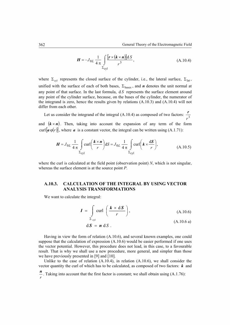
General Theory of the Electromagnetic Field 362
,d
4
1
cyl
30r
SJ L
nkrH (A.10.4)
where cyl represents the closed surface of the cylinder, i.e., the lateral surface, lat ,
unified with the surface of each of both bases, bases , and n denotes the unit normal at any point of that surface. In the last formula, Sd represents the surface element around any point of the cylinder surface, because, on the bases of the cylinder, the numerator of the integrand is zero, hence the results given by relations (A.10.3) and (A.10.4) will not differ from each other.
Let us consider the integrand of the integral (A.10.4) as composed of two factors: 3r
r
and nk . Then, taking into account the expansion of any term of the form
racurl , where a is a constant vector, the integral can be written using (A.1.71):
,d
curl4
1dcurl
4
1
cylcyl
00r
JSr
J LLS
knk
H(A.10.5)
where the curl is calculated at the field point (observation point) N, which is not singular, whereas the surface element is at the source point P.
A.10.3. CALCULATION OF THE INTEGRAL BY USING VECTOR ANALYSIS TRANSFORMATIONS
We want to calculate the integral:
.dd
,d
curl
cyl
S
r
nS
SkI (A.10.6)
(A.10.6 a)
Having in view the form of relation (A.10.6), and several known examples, one could suppose that the calculation of expression (A.10.6) would be easier performed if one uses the vector potential. However, this procedure does not lead, in this case, to a favourable result. That is why we shall use a new procedure, more general, and simpler than those we have previously presented in [9] and [10].
Unlike to the case of relation (A.10.4), in relation (A.10.6), we shall consider the vector quantity the curl of which has to be calculated, as composed of two factors: k and
r
n. Taking into account that the first factor is constant; we shall obtain using (A.1.76):

Appendix 10. The General Formula of the Magnetic Field Strength of a Solenoid.
363
( ) .divcurlrrrnknknk
∇⋅−=⎟⎠⎞
⎜⎝⎛ × (A.10.7)
The right-hand side contains a term that appears also in the expression of the gradient of the scalar product, one vector of which, namely k , is constant, and by (A.1.74) we get:
( ) ( ) .curlgrad 3 ⎟⎠⎞
⎜⎝⎛ ××+∇⋅=⎟
⎠⎞
⎜⎝⎛×+∇⋅=⎟
⎠⎞
⎜⎝⎛ ⋅
rrrrrrnknknknknk (A.10.8)
Therefore:
.divgradcurl 3 ⎟⎠⎞
⎜⎝⎛ ××+⎟
⎠⎞
⎜⎝⎛+⎟
⎠⎞
⎜⎝⎛ ⋅−=⎟
⎠⎞
⎜⎝⎛ ×
rrrrrnknknknk (A.10.9)
From relations (A.10.6) and (A.10.9), it follows that:
.
,dddivdgrad
baseslatcyl
3
cyl
SS
rrr
∪=Σ
⎮⌡
⌠⎥⎦
⎤⎢⎣
⎡⎟⎠⎞
⎜⎝⎛ ××++⎟
⎠⎞
⎜⎝⎛ ⋅−=
Σ
rSkSkSkI (A.10.10)
We shall calculate the component produced by each of the three terms contained by the integral.
The first term yields according to (A.1.169):
( ) ( ) ( ).ddddgrad
baseslatcylcyl
3331 ⎮⌡⌠ ⋅+⎮⌡
⌠ ⋅=⋅=⎮⌡⌠
⎟⎠⎞
⎜⎝⎛ ⋅−= ∫
ΣΣ SSrrrr
SkrSkrSkrSkI (A.10.11)
In the integral extended over the lateral surface of the cylinder, the scalar product Sk d⋅ is zero because the two vectors are, at any point of this surface, perpendicular to
each other. Hence:
( ).d
bases
31 ⎮⌡⌠ ⋅=
Sr
SkrI (A.10.12)
The second term yields according to (A.1.70):
.dddiv
cylcyl
32 ⎮⌡⌠ ⋅
−=⎮⌡⌠
⎟⎠⎞
⎜⎝⎛=
ΣΣrr
SrkSkI (A.10.13)
In order to simplify the calculation, we shall apply the theorem of Gauss-Ostrogradski for obtaining the transformation of a surface integral into a volume one. For applying the usual formulae containing differential operators, taking into account that the point N is fixed, we shall consider, when performing the calculation, the vector rr −=′ , and after

General Theory of the Electromagnetic Field 364
the calculation has been performed, we shall return to vector r. However, for conciseness reason, we shall not write this intermediary transformation.
In order to ensure the applicability of the mentioned theorem, we shall first separate, inside the cylinder, the singular point, that is the point corresponding to 0r , by surrounding it with a sphere, having the centre at that point, and small enough, so that it does not touch the cylinder. Then, we have to calculate the integral:
,,ddd
icyl333
icyl
rrr
SrSrSr
(A.10.14)
where i represents the surface of the sphere, which surrounds the singular point above. The above mentioned theorem yields:
.,0ddivd
icyl33
V
vrr
rSr
(A.10.15)
For the sphere surface, the unit normal is oriented, as in general, outwards the considered volume, that is, towards the sphere centre, as ir in A.10.1. Therefore, relations (A.10.14) and (A.10.15) yield:
.dd
icyl
33 rr
SrSr
(A.10.16)
The relations (A.10.13) and (A.10.16) yield:
.4dd
4i
ii32 k
rrk
SrkI S
rrii
(A.10.17)
If the point N is outside the cylinder, the term 2I is zero. The third term yields:
.d
cyl
33r
rSkI
(A.10.18)
It will be calculated similarly as the second one. Using the same definition of as in relation (A.10.14), we have:
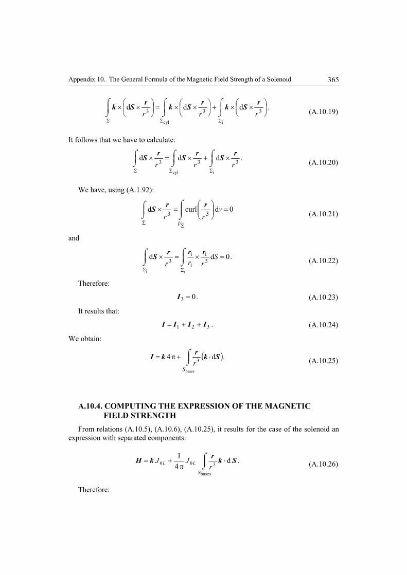
Appendix 10. The General Formula of the Magnetic Field Strength of a Solenoid. 365
.ddd
icyl
333 rrr
rSk
rSk
rSk
(A.10.19)
It follows that we have to calculate:
.ddd
icyl
333 rrr
rS
rS
rS
(A.10.20)
We have, using (A.1.92):
V
vrr
0dcurld33
rrS
(A.10.21)
and
.0dd
ii
3i
i
i3
Srrr
rrrS (A.10.22)
Therefore:
.03I (A.10.23)
It results that:
.321 IIII (A.10.24)
We obtain:
.d4
bases
3
Sr
Skr
kI (A.10.25)
A.10.4. COMPUTING THE EXPRESSION OF THE MAGNETIC FIELD STRENGTH
From relations (A.10.5), (A.10.6), (A.10.25), it results for the case of the solenoid an expression with separated components:
.d4
1
bases
300
S
LLr
JJ Skr
kH (A.10.26)
Therefore:

General Theory of the Electromagnetic Field 366
,,0;\,1;
;d4
1
cylcylcyl0
0
bases
300
VNmVNmh
iJ
rJJmN
S
L
S
LL Skr
kH
(A.10.27)
where the following symbols have been used: cylV – volume domain occupied by the
cylinder; cyl – cylinder surface; Sbases – surface of each cylinder base; i0 – total current
sheet; J0L – linear current density; k – unit vector along the cylinder generatrix; r –position vector of observation (field) point N with respect to the origin (source) point P.Therefore: if the point N is outside the cylinder, the first term of the right-hand side is zero, and if it is inside, it is different from zero.
The last formula emphasizes that, generally, the expression for any observation (field) point inside the cylinder has two components, the latter of Coulombian type and the former of non-Coulombian type. If the observation point is outside the cylinder, the former term vanishes, while the latter subsists.
It is interesting to emphasize that the last relation permits to establish a known general relation. If we change the symbols and denote the second term by NH the Coulombian component, and by M the value of the first non-Coulombian component, we can write:
,)()(1
0NNN HMB (A.10.28)
where, the quantity H has the character of the magnetic field strength, and the quantity M has the character of the magnetization. In general:
,00 MHB (A.10.29)
or introducing the magnetic polarization:
.0 jMHB (A.10.30)
If any other magnetic field, produced by other causes for instance electric currents, exists it has to be included into the vector H . Therefore, in such cases, the magnetic field strength may be of non-Coulombian type.
It follows that formula (A.10.27) allows for deducing the relation between the magnetic field strength, polarization and induction, in the general case. If any substance contains a large number of elementary solenoids, the relations above are valid for the quantities BMH ,, of every solenoid and also for the average of these quantities over any physically infinitesimal interval of space and time. We have, hence, found anew, simpler and in a more general way a result of paper [9] and [10].

Appendix 10. The General Formula of the Magnetic Field Strength of a Solenoid. 367
A.10.5. CALCULATION OF THE MAGNETIC FIELD STRENGTH PRODUCED BY A CIRCULAR CROSS-SECTION SOLENOID BY USING DIRECTLY THE BIOT-SAVART-LAPLACE FORMULA
In order to verify the accuracy of formulae above, we shall apply formula (A.10.3) forcalculating the magnetic field strength of a right circular cylinder. We shall consider theconfiguration of Fig. A.10.1, and use formula (A.10.3). It will be recalled that P is thesource point, whereas N is the observation (field) point. For applying the formula, weshall consider a slice of the cylinder, of a very small height z. Let NNN zyx ,, be the
co-ordinates of point N, and, 1bz and 2bz , the z-co-ordinates of the two bases of thecylinder. The slice will be taken at any co-ordinate z. For simplicity, without restrictingthe generality, we shall take 0Ny .
The projection of the considered slice on the plane xOy is shown in Fig. A.10.2.The product rl will be expressed by using the polar co-ordinates and where,
in this case, 0r . It follows:
Fig. A.10.2. The projection of the circumference of a cross-section of the solenoid cylinder on the xOy - plane: The representation of the projection ofthe position vector PN using polar co-ordinates. The segment OP belongs to the
plane of the circle.
,0cossin 00 kjil rr (A.10.31)
,sincos 00 zzrrx NN kjir (A.10.32)
2 r
xx Nx
P
N
y
P
Py
O
l

General Theory of the Electromagnetic Field 368
.cossincos 0000 rxrrzzrzz NNN kjirl (A.10.33)
The utilization of formula (A.10.31) results in calculating a double integral with respect to variables z and , for each of the three axes of Cartesian co-ordinates.
Taking into account that, for reasons of symmetry, yH is zero, it results that:
,4
1;d2;0;d2 00
00
rJfIfHHIfH Lzzyxx(A.10.34 a,..,d)
where, in order to shorten the explanations, we shall use the following symbols:
;dcos
;dcos
2b
1b
2b
1b
30
3
z
z
z
z
Nz
Nx z
r
xrIz
r
zzI (A.10.35)
and
.cos2 2
12
02
02 zzrxrxr NNN
(A.10.36)
We shall denote:
.)( 22 zzcarzFF N (A.10.37)
For the calculation of expressions (A.10.35 a, b), we can use one of the procedures of Sub-Section A.10.6.1. For this purpose, we shall denote:
.dd;;44
;1;0;cos2 200
2
zzxzzxacaD
cbrrxxa
NN
NN (A.10.38 a-f)
We get:
.cos4
,cos1
0
2b
1b
2b
1b
N
z
z
Nz
z
z
x
xrFD
zzI
FI (A.10.39)
(A.10.40)
Then, we shall calculate the integrals (A.10.34 a, c) above, with respect to the variable . This calculation has been carried out by a numerical method, using the Gauss integration method, by a procedure with 32-point ordinates.

Appendix 10. The General Formula of the Magnetic Field Strength of a Solenoid. 369
A.10.6. CALCULATION OF THE MAGNETIC FIELD STRENGTH PRODUCED BY A CIRCULAR CROSS-SECTION SOLENOID BY USING THE FORMULA WITH SEPARATE COMPONENTS
In order to verify the accuracy of formulae above, we shall apply formula (A.10.27)for calculating the magnetic field strength of a right circular cylinder. We shall considerthe configuration of Fig. A.10.1, and use formula (A.10.27). We shall consider, theconfiguration of Fig. A.10.3. It will be recalled that, as previously, P is the source point,whereas N is the observation (field) point.
Fig. A.10.3. The projection of a thin slice of the end of the solenoid cylinder on thexOy - plane: The representation of the projection of the position vector PN using
polar co-ordinates. The segment OP belongs to the plane of the circle.
Let, as above, NNN zyx ,, be the co-ordinates of point N, and, 1bz and 2bz , be thez-co-ordinates of the two bases of the cylinder. For simplicity, without restricting the
generality, we shall take 0Ny . For describing the position of a point on each of thetwo bases of the solenoid cylinder, polar co-ordinates and will be used, as inFig. A.10.3. The vector oriented from point P to point N will be:
.sincos zzx NN kjir (A.10.41)
The calculation by formula (A.10.27) results in calculating a double integral withrespect to variables and , for each of the three axes of Cartesian co-ordinates.
Taking into account that, for reasons of symmetry, yH is zero, it results that:
y
Py P
O
2 r
N
x N x
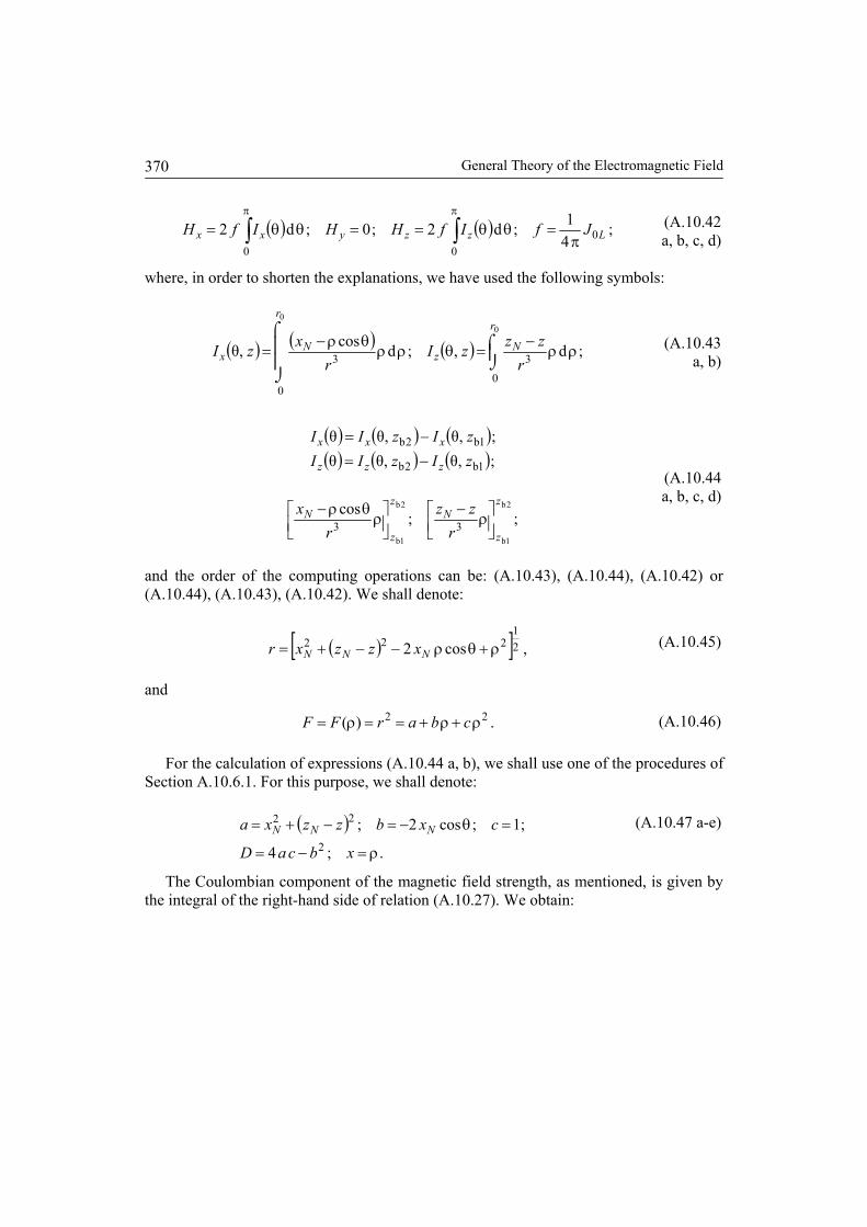
General Theory of the Electromagnetic Field
370
( ) ( ) ;41;d2;0;d2 0
00Lzzyxx JfIfHHIfH
π=θθ==θθ= ∫∫
ππ
(A.10.42 a, b, c, d)
where, in order to shorten the explanations, we have used the following symbols:
( ) ( ) ( ) ;d,;dcos,θ
00
00
33⎮⎮
⌡
⌠⎮⌡⌠ ρρ
−=θρρ
θρ−=
rr
Nz
Nx r
zzzIr
xzI (A.10.43 a, b)
( ) ( ) ( )( ) ( ) ( );,θ,θθ
;,θ,θθ
1b2b
1b2b
zIzIIzIzII
zzz
xxx
−=−=
;;cos 2b
1b
2b
1b33
z
z
Nz
z
N
rzz
rx
⎥⎦⎤
⎢⎣⎡ ρ
−⎥⎦⎤
⎢⎣⎡ ρ
θρ−
(A.10.44a, b, c, d)
and the order of the computing operations can be: (A.10.43), (A.10.44), (A.10.42) or (A.10.44), (A.10.43), (A.10.42). We shall denote:
( )[ ] ,cos2 21
222 ρ+θρ−−+= NNN xzzxr (A.10.45)
and
.)( 22 ρ+ρ+==ρ= cbarFF (A.10.46)
For the calculation of expressions (A.10.44 a, b), we shall use one of the procedures of Section A.10.6.1. For this purpose, we shall denote:
( ).;4
;1;cos2;2
22
ρ=−=
=θ−=−+=
xbcaD
cxbzzxa NNN (A.10.47 a-e)
The Coulombian component of the magnetic field strength, as mentioned, is given by the integral of the right-hand side of relation (A.10.27). We obtain:
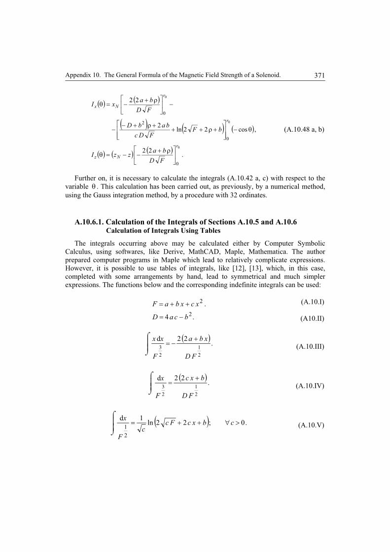
Appendix 10. The General Formula of the Magnetic Field Strength of a Solenoid. 371
.22
,cos22ln2
22
0
0
0
0
0
2
0
r
Nz
r
r
Nx
FD
bazzI
bFFDc
babD
FD
baxI
(A.10.48 a, b)
Further on, it is necessary to calculate the integrals (A.10.42 a, c) with respect to the variable . This calculation has been carried out, as previously, by a numerical method, using the Gauss integration method, by a procedure with 32 ordinates.
A.10.6.1. Calculation of the Integrals of Sections A.10.5 and A.10.6 Calculation of Integrals Using Tables
The integrals occurring above may be calculated either by Computer Symbolic Calculus, using softwares, like Derive, MathCAD, Maple, Mathematica. The author prepared computer programs in Maple which lead to relatively complicate expressions. However, it is possible to use tables of integrals, like [12], [13], which, in this case, completed with some arrangements by hand, lead to symmetrical and much simpler expressions. The functions below and the corresponding indefinite integrals can be used:
.4
.2
2
bcaD
xcxbaF (A.10.I)
(A10.II)
.22d
2
1
2
3
FD
xba
F
xx(A.10.III)
.22d
2
1
2
3
FD
bxc
F
x(A.10.IV)
.0;22ln1d
2
1cbxcFc
cF
x(A.10.V)

General Theory of the Electromagnetic Field372
.22ln12d
2
1
2
2
3
2
bxccFcc
FDc
xbDba
F
xx(A.10.VI)
A.10.7. COMPUTER PROGRAMS AND NUMERICAL RESULTS
For the methods developed in the present paper, we have developed computerprograms in Fortran.F77 language. For integration by the Gauss method, the subroutineDQG32 of the IBM Library has been used. The program has been written in doubleprecision, that is, each word has two bytes, i.e., 16 bits, what ensures results of highprecision even at points in the vicinity of singular points. The obtained results are givenin Table 1. The programs are called SOLENBSL.F77 based on the Biot-Savart-Laplaceformula, and SOLENCNC.F77 based on the separated components formula.
If the two types of formulae ensure a good accuracy, they have to give results veryclose to each other. We have compared the results for various points placed at variouspositions with respect to the cylinder. The greatest relative deviation has been of the order
of magnitude of 510 .Table 1
Results obtained by numerical computation of the magnetic field strength by three methods:
1. Biot-Savart-Laplace formula. 2. Formula with the separated Coulombian components.
3. Formula in closed form. Data of the solenoid: 11bz , 12bz , 10r , 10LJ .
a. Co-ordinates of the observation point: 0Nx , 0Ny . Component zH .
Value of zN
and method-1.01 -1
(-1.0000001)-0.5 0 0.5 1
(1.0000001)
1 0.4016784E+00
0.4472135E+00
0.6396319E+00
0.7071068E+00
0.6396319E+00
0.4472135E+00
2 0.4016784E+00
0.4472135E+00
0.6396319E+00
0.7071068E+00
0.6396319E+00
0.4472135E+00
3 0.4016784E+00
0.4472136E+00
0.6396319E+00
0.7071068E+00
0.6396319E+00
0.4472135E+00
b. Co-ordinates of the observation point: 2Nx , 0Ny . Component zH .
Value of zN
and method-1.5 -1 -0.5 0 0.5 1
1 -0.458168E-03
-0.224792E-01
-0.440966E+00
-0.518527E+00
-0.440966E-01
-0.224792E-01
2 -0.458168E-03
-0.224972E-01
-0.440966E+00
-0.518527E+00
-0.440966E-01
-0.224792E-01
c. Co-ordinates of the observation point: 2Nx , 0Ny . Component xH .
Value of zN
and method-1.5 -1 -0.5 0 0.5 1
1 -0.466422E-01
-0.489889E-01
-0.305329E-01
0.000000E+00
0.305329E-01
0.489889E-01
2 -0.466422 -0.489889 -0.305329 0.000000 0.305329 0.489889

Appendix 10. The General Formula of the Magnetic Field Strength of a Solenoid. 373
The obtained results show a small difference between the two methods, these are due to the rounding error, different for each formula. It has to be noted that the errors are very small even in the neighbourhood of singular points. Afterwards has remade the computation using the Maple 12 software, for the case in which we are not interested in the simplicity of the form of formulae. We could realize certain programming facilities
and greatest relative deviation has been of the order of magnitude of less than 710 . In the table above, there are given the last results, for this reason no deviation appears, which appeared in the foregoing papers of the author. The comparison of the results obtained using by formulae in closed form and numerical procedures, respectively, has shown that, at least, the first seven digits of the mantissa (or significant), the results being written in the form of the table above, coincide.
A.10.8. CALCULATION OF THE MAGNETIC FIELD STRENGTH OF A SOLENOID BY USING FICTITIOUS MAGNETIC CHARGES
We shall consider two space domains of the same form and sizes, both of finite length, containing a cylindrical solenoid and a uniformly magnetically polarized cylinder.
The cylindrical solenoid produces a magnetic field as well as the cylindrical uniformly magnetically polarized body occupying the same domain. According to paper [9], a cylindrical solenoid may be decomposed in a set of elementary solenoids, the neighbouring current sheets of which being of similar directions, their effect will be the same as that of the given solenoid. At the same time, according to the same paper, the cylindrical uniformly magnetized cylinder may be decomposed in a set of elementary magnetic dipoles. If one magnetic dipole is equivalent to one elementary solenoid, then the magnetic field produced by each of them in their neighbourhood will be the same. According to the same paper, at a microscopic scale, the magnetic field strength of elementary dipole and elementary solenoid have different values. Then, if we consider a single cylindrical solenoid and a single magnetized cylinder, the magnetic field strength inside the considered domains will be also different, regardless of the cylinder size, hence microscopically as well as macroscopically. But, the magnetic induction will be the same in both cases. Therefore, we shall consider the magnetic induction of the two domains.
In the case of the magnetically polarized cylinder of finite length, the magnetic field strength may be obtained by using the principle of superposition, like in paper [9]. The considered magnetically polarized cylinder will be considered as belonging to an infinitely long cylinder. We can consider that the infinitely long cylinder consists of three parts: the considered cylinder of finite length, and other two semi-infinite cylinders, each of them situated on one part of the cylinder of finite length, in order to built-up the whole infinitely long cylinder.
The magnetic induction (flux density) at any point inside or outside the cylinder of finite length will have two components:
1. A component, say of type a, produced by the infinitely long cylinder. Because the effect of magnetic dipoles cancels each other, the volume density of the fictitious magnetic charge will be zero, and the magnetic field strength produced by
General Theory of the Electromagnetic Field
374
the infinite cylinder will be zero, inside as well outside the cylinder, but the magnetic induction will be different from zero inside, and zero outside.
2. A component, say of type d, produced by the two semi-infinite cylinders, each of them situated on one side of the cylinder of finite length, taken with changed sign, because it has to be subtracted from the previous one.
Because the effect of magnetic dipoles cancels each other, the volume density of the fictitious magnetic charge will be zero, and only the fictitious magnetic charge of the base of the semi-infinite cylinder will contribute to the production of a magnetic field.
The component of type a will be:
( ) ,a jN MB = (A.10.49 a)
inside, and
( ) ,0a =NB (A.10.49 b)
outside the infinite cylinder. The magnetic induction produced at any point inside as well as outside the cylinder of
finite length will be given by the known relation (like in Electrostatics):
( ) ,d41
bases
3d ⎮⌡⌠ ⋅
π=
S
jrN SMrB (A.10.50)
where not minus sign has to be introduced, because the integral limits above refer to the cylinder of finite length, and the normals to the bases of this cylinder are opposite to those on the bases of the semi-infinite length.
By summing up the formulae (A.10.49) and (A.10.50), dividing by the permeability of vacuum both sides, and replacing, the magnetic polarization, according to formulae (14), (18) of [9], we have just formula (A.10.27) above.
This latter deduction has not the generality of the former one, but, in turn, it has the advantage of being suggestive.
A.10.9. CONCLUSION
The presented new method of establishing the magnetic field strength of a solenoid calculating the magnetic field strength produced by a right cylindrical solenoid of finite length and with a cross-section of any form has the advantage of using only the Vector Analysis formulae, without resorting to the method of fictitious magnetic charges or to general formulae of the field theory. The method leads to an expression with separated components. The obtained expression permits the calculation of the magnetic field strength produced by various form of the solenoid, is easier to be applied than other largely used expressions and ensures a high accuracy. Also, it permits to obtain directly the relation between induction (flux density), field strength and polarization of a magnetic field. Certain results concerning the usage of various softwares have been obtained, what has not been known in other publications.

Appendix 10. The General Formula of the Magnetic Field Strength of a Solenoid.
375
List of Symbols Used in Appendix 10
B – macroscopic magnetic induction; ld – line element vector; Sd – Surface element vector;
H – macroscopic magnetic field strength;
Sh – length of a cylinder that can be a solenoid or a uniformly magnetized body;
I – symbol of any vector integral with a certain suffix; kji ,, – unit vectors of a three-orthogonal right-handed system of co-ordinates;
i – electric current intensity;
0i – total electric current intensity of a solenoid;
LJ0 – linear density of the current sheet of a solenoid;
k – unit vector of the generatrix of a right cylinder; M – magnetization vector;
jM – MM 0µ=j , magnetic polarization vector; n – unit vector of the normal to a surface; r – position vector of any observation (field) point P relatively to the origin or
source point N; ir – radius of the interior sphere with the centre at the observation point;
0r – radius of the cylinder; zyx ,, – co-ordinates of any source point P;
,Nx
NN zy ,
– co-ordinates of any observation point N;
,1bz
2bz
– co-ordinate along the Oz-axis of the two bases of the cylinder;
S – open surface that can have a suffix indicating it; Γ – curve, in most cases, a closed one; µ – magnetic permeability, in vacuo it is 0µ ; θ – angle in cylindrical co-ordinates; Σ – closed surface that can contain a suffix indicating it.
REFERENCES
1. MAXWELL, J.C.: A Treatise on Electricity and Magnetism, Third Edition, Clarendon Press, London, 1891. Reprinted by Dover Publications, Inc., New York, 1954.
2. DURAND, É.: Magnétostatique, Masson et C-ie, Éditeurs, Paris, 1968. 3. FAWZI, T.H., BURKE, P.E.: The accurate computation of self and mutual inductances of
circular coils. IEEE Transactions on PAS, vol. 97, No. 2 (1978), pp. 464-468. 4.
FOURNET, G.: Électromagnétisme à partir des équations locales, Masson et C-ie,
Éditeurs,Paris, 1985. 5. BABIC, S., et al.: Calculation improvement of 3D linear magnetostatic field based on
fictitious magnetic surface charge. IEEE Trans. Magn., vol. 36, No. 5 (2000), pp. 3125-3127.
General Theory of the Electromagnetic Field
376
6. BABIC, S., et al.: The mutual inductance of two thin coaxial disk coils in air. IEEE Trans. Magn., vol. 40, No. 2 (2004), pp. 822-825.
7. MORARU, A.: Bazele electrotehnicii. Teoria câmpului electromagnetic (Fundamentals of Electrotechnics. Theory of the electromagnetic field). Edit. Matrix Rom, Bucharest, 2002.
8. NICOLAIDE, A.: Electromagnetics. General Theory of the Electromagnetic Field, Second Edition, Transilvania University Press, Braşov 2009.
9. NICOLAIDE, A.: A New Analysis of the Introduction of the Magnetic Field State Quantities in Solids. Periodica Polytechnica Ser. El. Eng. Vol. 48, No. 3 (2004), pp. 101-118.
10.
NICOLAIDE, A.: Establishing a general formula of the magnetic field strength of a solenoid. Rev. Roum. Sci. Techn. – Électrotechnique et Énergétique, 49, No. 3, (2004), pp. 295-308.
11. NICOLAIDE, A.: A new approach to the introduction of the electric and magnetic field state quantities. Rev. Roum. Sci. Techn. – Électrotechnique et Énergétique, 49, No. 4 (2004), pp. 547-560.
12. RYZHIK, I.M., GRADSTEIN, I.S.: Tables of Series, Products, and Integrals, Second Edition. New York: Plenum Press, 1963.
13. FRENET, F.: Recueil d’exercisses sur le calcul infinitesimal. Gauthier-Villars et C-ie, Éditeurs, Paris, 1917.
14. SCHEIBER, E., LUPU, M.: Matematici speciale. Rezolvarea problemelor cu ajutorul calculatorului (Special Mathematics. Solving Problems by Computer), Edit. Tehnică, Bucureşti, 1998.
15. NICOLAIDE, A.: Transforming the Expression of the Integral of a Vector Field Curl over a Cylinder Surface into Another Surface Integral without Differential Operators. In: World Congress on Engineering 2008, IAENG International Association of Engineers, The 2008 International Conference of Applied and Engineering Mathematics, London, 2-4 July, 2008, Vol. II, pp. 918-921. ISBN: 978-988-17012-3-7.
16. NICOLAIDE, A.: A New Vector Analysis Approach to the Calculation of the Magnetic Field Strength of a Solenoid. Current Themes in Engineering Science 2008. Editor: Alexander M. Korsunsky. Melville, New York, 2009, American Institute of Physics. AIP Conference Proceedings, volume 1138, pp. 59-70.
17. **
* Maple 12. The Essential Tool for Mathematics and Modeling. Maplesoft, a division of Waterloo Maple Inc. 1996-2008.

BIBLIOGRAPHY A. Treatises, Textbooks and Works on Electromagnetism
1. MAXWELL, J.C.: A Treatise on Electricity and Magnetism. Third Edition, London: Clarendon Press, 1891. Reprinted by Dover Publications, Inc., New York, 1954.
2. LORENTZ, H.A.: Theory of Electrons and Its Applications in the Phenomena of Light and Radiant Heat. Teubner Publishing Company, Leipzig, 1909. Reprinted by Dover Publications, Inc., New York, 1952.
3. BLOCH, L.: Précis d‘Électricité Théorique. Gauthier-Villars et C-ie, Éditeurs, Paris, 1919.
4. PROCOPIU, Şt.: Electricitate şi magnetism (Electricity and Magnetism). Vol. I. Editura Laboratorului de electricitate, Iaşi, 1942.
5. SMYTHE, W.R.: Static and Dynamic Electricity. McGraw-Hill Book Company, New York, 1950.
6. DACOS, F.: Conception actuelle de l‘électricité théorique. Dunod, Éditeur, Paris, 1957.
7. TAMM, I.E.: Bazele teoriei electricităţii. Editura Tehnică, Bucureşti, 1957. Fundamentals of the Theory of Electricity. Mir Publishers, Moscow, 1979.
8. RĂDULEŢ, R.: Bazele teoretice ale Electrotehnicii (Theoretical foundations of Electrotechnics). Vol. I-IV. Litografia Institutului Politehnic Bucureşti, 1958.
9. *** Manualul inginerului electrician (Handbook of the electrical engineer). Vol. I, Editura Tehnică, Bucureşti, 1958.
10. FOURNET, G.: Physique électronique des solides à l’usage des ingénieurs (École Nationale Supérieure des Télécommunications). Éditions Eyrolles, Paris, 1962.
11. ARZELIÈS, H.: Électricité. Le point de vue macroscopique et relativiste. Gauthier-Villars, Éditeur, Paris, 1963.
12. DURAND, É.: Électrostatique. Tome I – Les distributions. Tome II – Problèmes généraux. Tome III – Méthodes de calcul. Diélectriques. Masson et C-ie, Éditeurs, Paris, 1964, 1966, 1966.
13. ELLIOTT, R.S.: Electromagnetics. McGraw Hill Company, New York, 1966. 14. BRUHAT, G.: Cours de Physique Générale. Électricité. Huitième édition revisée
par G. GOUDET. Masson et C-ie, Éditeurs, Paris, 1967. 15. DURAND, É.: Magnétostatique. Masson et C-ie, Éditeurs, Paris, 1968. 16. BESSONOW, A.: Applied Electricity for Engineers. Mir Publishers, Moscow, 1968. 17. LANDAU, L.D., LIFSHITZ, E.M.: Electrodynamics of Continuous Media, Course of
theoretical Physics. Vol. 8, Pergamon Press, Oxford, 1960. Fizică teoretică. Electrodinamica mediilor continue. Editura Tehnică, Bucureşti, 1968.

Bibliography
378
18. ROSSER, W.G.V.: Classical Electromagnetism Via Relativity. Edit. Butterworths, London, 1968.
19. PHILIPPOW, E.: Grundlagen der Elektrotechnik. Akademische Verlagsgesellschaft Geest & Portig K.- G., Leipzig, 1970.
20. VALLÉE, R.L.: L’énergie électromagnétique materielle et gravitationnelle. Hypothèse de l’existence des milieux énergétiques et d’une valeur limite supérieure du champ électrique. Masson et C-ie, Éditeurs, Paris, 1971.
21. FOURNET, G.: Électromagnétisme à partir des équations locales. Masson et C-ie, Éditeurs, Paris, 1985.
22. FISCHER, J.: Elektrodynamik. Springer-Verlag, Berlin, Heidelberg, New York, 1975.
23. NICOLAIDE, A.: Bazele fizice ale Electrotehnicii (Physical foundations of Electrical Engineering). Vol. I, Vol. II, Editura Scrisul Românesc, Craiova, 1983, 1986.
24. NOVOZHILOV, Yu., YAPPA, A.: Electrodynamics. Mir Publishers, Moscow, 1986. 25. ELLIOTT, R.S.: Electromagnetics: History, Theory, and Applications. The IEEE
Press, 1993. 26. NICOLAIDE, A.: Magnetism and Magnetic Materials. Transilvania University Press,
Braşov, 2001.
B. Works on Electromagnetism and the Theory of Relativity 27. EINSTEIN, A.: The Meaning of Relativity. Princeton University Press, Princeton,
New Jersey, 1955. Teoria relativităţii. Editura Tehnică, Bucureşti, 1957. 28. SAGNAC, G.: Sur les interférences des deux faisceaux superposés en sens invers le
long d‘un circuit optique de grandes dimensions. Comptes Rendus de l‘Académie des Sciences. Séance du 23 mai 1910, T. 150, No. 21, pp. 1302-1305. Paris, 1910.
29. SAGNAC, G.: Interféromètre à faisceaux lumineux superposés inverses donnant en lumière blanche polarisée une frange centrale étroite à teinte sensible et des franges colorées étroites à intervalles blancs. Comptes Rendus de l‘Académie des Sciences. Séance du 13 juin 1910, T. 150, pp. 1676-1679.
30. SAGNAC, G.: L‘éther lumineux démontré par l‘effet du vent relatif d‘éther dans un interféromètre en rotation uniforme. Comptes Rendus de l‘Académie des Sciences. Séance du 27 octobre 1913. T. 157, pp. 708-710.
31. SAGNAC, G.: Sur la preuve de la réalité de l‘éther lumineux par l‘expérience de l‘interférographe tournant. Comptes Rendus de l‘Académie des Sciences. Séance du 22 décembre 1913. T. 157, pp. 1410-1413.
32. ARZELIÈS, H.: La cinématique relativiste. Gauthier-Villars, Éditeur, Paris, 1955. 33. ARZELIÈS, H.: La dynamique relativiste. Gauthier-Villars, Éditeur, Paris, 1957. 34. KELLY, A.G.: Time and the Speed of Light – a New Interpretation. The Institution
of Engineers of Ireland, Monograph No. 1, January 1995. 35. KELLY, A.G.: A New Theory on the Behaviour of Light. The Institution of
Engineers of Ireland, Monograph No. 2, February 1996. 36. KELLY, A.G.: Reliability of Relativistic Effect Tests on Airborne Clocks. The
Institution of Engineers of Ireland, Monograph No. 3, February 1996.
Bibliography
379
37. MONSARRAT, B.: La Relativité: Une conséquence de la structure Quadridimensionnelle de l’univers. Conférence. Organisation: SEE – Société des Électriciens et Électroniciens, Supelec (École Supérieure d’Électricité), 12 octobre 1998.
38. FABRE, L.: Une nouvelle figure du monde. Les Théories d’Einstein. Payot et C-ie, Paris, 1922.
39. POINCARÉ, H.: La mécanique nouvelle. Conférence, mémoire et note sur la Théorie de la relativité. Les grands classiques. Gauthier-Villars et C-ie, Éditeurs, Paris, 1924. Éditions Jacques Gabay, Paris, 1989.
40. NICOLAIDE, A.: Grundlagen für eine Ableitung der Gleichungen des elektromagnetischen Feldes unter Anwendung der Speziellen Relativitätstheorie (Foundations of the Derivation of the Electromagnetic Field Equations by Applying the Special Theory of Relativity). Archiv für Elektrotechnik, 1974, Bd. 56, H. 3, S. 149-155. Springer-Verlag, Berlin, Heidelberg, New York.
41. NICOLAIDE, A.: Ableitung der Gleichungen des elektromagnetischen Feldes unter Anwendung des Coulombschen Gesetzes und der Speziellen Relativitätstheorie. (Derivation of the Electromagnetic Field Equations by Applying Coulomb’s Law and the Special Theory of Relativity). Archiv für Elektrotechnik, 1974, Bd. 56, H. 3, S. 156-160. Springer-Verlag, Berlin, Heidelberg, New York.
C. Standards 42. ***Sistemul internaţional de unităţi (SI). Mărimi caracteristice ale
electromagnetismului. Unităţi de măsură. (The International System of Units (SI). Characteristic quantities in electromagnetism. Units of measure). State Standard STAS 737/9-74.
43. ***Mărimi în electrotehnică. Simboluri (Quantities in Electrotechnics. Symbols). State Standard STAS 3087-76.
44. Norme Internationale CEI 27-1, Sixième édition, 1992-12. Symboles littéraux à utiliser en électrotechnique. Partie 1: Generalités. International Standard IEC 27-1, Sixth edition 1992-12. Letter symbols to be used in electrical technology. Part 1: General. Genève, 1999.
45. Norme Internationale CEI 60027-1, 1992, Amendement 1, 1997-05. Symboles littéraux à utiliser en électrotechnique. Partie 1: Généralités. International Standard IEC 60027-1, 1992, Amendment 1, 1997-05. Letter symbols to be used in electrical technology. Part 1: General. Genève, 1999.
46. CARPENTIER, J.: Le système international d’unités en 1992 (The International System of Units in 1992). In: Revue Générale de l’Électricité, 1993, No. 5, pp. 1-9, Paris.
47. KOSOW, I.L.: Circuit Analysis. Chapter 1: The SI, Scientific Notation, Unit Conversion, p. 1. Chapter 2: Current and Voltage, p. 15. Chapter 11: Magnetism and Magnetic Circuits, p. 278. Edit. John Wiley and Sons, New York, 1988.

Bibliography
380
D. Treatises, Textbooks and Works on Parts of Electromagnetism 48. KIRÉEV, V.: Cours de Chimie Physique. Éditions Mir, Moscou, 1968. 49. NICOLAIDE, A.: Significance of the scientific research of Nicolae Vasilescu Karpen
(1870-1964). AGIR Publishing House, Bucharest, 2006. 50. ŠPOLSKIJ, E.V.: Fizică atomică (Atomic Physics). Vol. I, II. Editura Tehnică,
Bucureşti, 1953. 51. TAREEV, B.M. et al.: Electrical and Radio Engineering Materials. Mir Publishers,
Moscow, 1980. E. Mathematical Methods 52. BRICARD, R.: Le Calcul vectoriel. Collection Armand Colin (Section de
Mathématiques). Librairie Armand Colin, Paris, 1932. 53. MORSE, P.M., FESHBACH, H.: Methods of Theoretical Physics. Part I, Part II,
McGraw-Hill Book Company, New York, 1953. 54. KOCIN, N.E.: Calculul vectorial şi introducere în calculul tensorial. (Vector
Calculus and introduction to Tensor Calculus). Editura Tehnică, Bucureşti, 1954.
F. Additional References 55. NICOLAIDE, A.: A new approach to the introduction of the electric and magnetic
field state quantities. Revue Roumaine des Sciences Techniques – Série Électrotechnique et Énergétique, 2004, 49, 4, pp. 547-560, Bucarest.
56. NICOLAIDE, A.: A new Analysis of the Introduction of the Magnetic Field State Quantities in Solids. Periodica Polytechnica, Ser. El. Eng., 2004, Vol. 48, No. 3, pp. 101-118, Budapest.
57. NICOLAIDE, A.: Establishing a general formula of the magnetic field strength of a solenoid. Rev. Roum. Sci. Techn. – Électrotechn. et Énerg., 2004, 49, 3, pp. 295-308, Bucarest.
58. NICOLAIDE, A.: Transforming the Expression of the Integral of a Vector Field Curl over a Cylinder Surface into Another Surface Integral without Differential Operators. World Congress on Engineering 2008, IAENG International Association of Engineers, The 2008 International Conference of Applied and Engineering Mathematics, London, 2-4 July, 2008, Vol. II, pp. 918-921, ISBN: 978-988-17012-3-7.
59. NICOLAIDE, A.: A New Approach for Establishing the Energy Momentum Tensor in the Theory of Relativity. World Congress on Engineering 2009, IAENG International Association of Engineers, The 2009 International Conference of Applied and Engineering Mathematics, London, 1-3 July, 2009, Vol. II, pp. 1131-1137, ISBN: 978-988-18210-1-0.
60. NICOLAIDE, A., PANAITESCU, A.: The energetic properties of the electromagnetic field. Dynamic properties of the electromagnetic field. Rev. Roum. Sci. Techn. – Électrotechn. et Énerg., 2008, 53, 2, 3, pp. 121-136, 239-252, Bucarest.
SUBJECT INDEX Ampere, unit of measure, p. 95. Ampère law, p. 143. Ampere-turns, p. 145. Amperian electric current, p. 76. Amperian magnetic charge, p. 169. Amperian magnetic moment, p. 78. Atom, p. 38, 50. Average value, p. 39. Average value of E, p. 50. Average value of electric polarization, p. 61. Average value, denoting, calculating,
p. 39, 48. Axial vector, p. 31. Base (basic) units, p. 30. Biot-Savart-Laplace formula, p. 115, remark on, p.116, law, p. 115. Bound electric charges, p. 43, 56. Cartesian system of co-ordinates,
p. 32, 101, 206. Cavity within a body, p. 61, 78. Charge carrier, p. 47. Charge of electron, p. 38. Circulation of a vector, p. 54, 219. Closed curve, simply closed curve, p. 35. Condition of electromagnetic field, p. 143. Conduction electric current, p. 72. Conductive (conducting) material, p. 42. Conductor, p. 45. Conservation of the normal component of
the electric displacement, p. 156. Conservation of the normal component of
the magnetic induction, p. 160. Conservation of the tangential component
of the electric field strength, p. 159. Conservation of the tangential component
of the magnetic field strength, p. 163. Conservation of the true electric charge,
p. 48, 80, 81, 83. Constant charge principle, p. 46. Contraction of lengths, p. 103. Contravariant quantity (tensor), p. 105. Convection electric current, p. 142. Coulomb formula for electric charges, p. 85,
in the special theory of relativity, p. 98. Coulomb formula for magnetic charges,
p. 169.
Coulomb formula, law, theorem, p. 86. Coulomb, unit of measure, p. 93. Coulombian electric field strength, p. 53. Coulombian magnetic charge, p. 169. Coulombian magnetic moment, p. 78. Covariant quantity (tensor), p. 105. Crystalline lattice, p. 43, 72. Curl of a vector, p. 219. Curl solenoidal field, p. 33. Curl component of the electric field strength,
p. 53, 112. Curl field, p. 33. Current-linkage, p. 145. Cylindrical co-ordinates, p. 242. Delocalized electron, p. 42. Density of amperian electric current, p. 79. Density of electric charge, p. 47. Density of electric current in terms of the
volume density of electric moving charge carriers, p. 70.
Density of the electric current, p. 69, 70. Density of the polarization electric charge,
volume density, p. 59, surface density, p. 60, 64, line density, p. 60.
Density of the surface tension, p. 200. Derivative of a scalar function with respect
to a given direction, p. 212. Derivative of a vector along a direction,
p. 224. Derivative with respect to time of the flux
through a moving open surface, p. 235. Derived quantity, p. 37. Derived unit, p. 37. Dielectric, p. 42. Dielectric constant, p. 124. Differential, exact, total, p. 89, 210. Differential operations by the nabla operator,
p. 227. Differential operations of the second order,
p. 229. Differential operators in curvilinear
co-ordinates, p. 242. Dilatation of time, p. 104. Dilation of time, p. 104. Dimension attributed to an atom, p. 50. Dimension attributed to an electron, p. 51.

Subject Index
382
Dipole (electric dipole), p. 58. Direction, p. 32. Displacement electric current, p. 145. Divergence and the curl of a vector by
means of the nabla operator, p. 226. Divergence of a vector, p. 215. Double vector product (of three vectors),
p. 207. Doublet (electric doublet), p. 58. Einstein postulates and theory, p. 99. Electric charge, p. 46. Electric conductivity, p. 83. Electric conductor, p. 45. Electric constant, p. 85, 107. Electric current, p. 68. Electric currents, action and reaction, p. 116. Electric displacement, in vacuo, and in any
medium, p. 108, 121, 123. Electric displacement, p. 121, 123. Electric field, p. 45. Electric field intensity, p. 53. Electric field line, p. 53. Electric field strength, in vacuo, p. 49, 85. Electric field strength, induced, rotational
solenoidal, curl component, p. 53, 112. Electric field strength in the large sense,
p. 52, 53. Electric field strength in the restricted sense,
p. 53. Electric field strength in various reference
frames, p. 107. Electric field strength produced by a
distribution of electric charges at rest, p. 87.
Electric flux, p. 122. Electric flux density, p. 108, 121, 123. Electric induction, p. 108, 121, 123. Electric insulator, p. 45. Electric moment of a neutral system, p. 57,
of a polarized body, p. 58. Electric polarization vector, p. 60. Electric potential difference, p. 88. Electric potential produced by charges
at rest, p. 87. Electric resistivity, p. 83. Electric tension, p. 55, 88. Electric tension in the large sense, p. 55. Electric tension in the restricted sense,
p. 55. Electrification by friction, p. 44. Electrification state, p. 44.
Electrodynamic potentials, p. 179. Electrodynamic potentials produced by one
electric charge moving at constant velocity, p. 183.
Electrodynamic potentials produced by one electric charge moving at non-constant velocity, p. 185.
Electrodynamic vector potential, p. 179. Electromagnetic momentum, p. 200. Electromagnetic System of Units, p. 168. Electromotive force, p. 55. Electromotive force in the large sense,
p. 55. Electromotive force in the restricted sense,
p. 55. Electromotive force induced by the rotation
of a magnet about its axis, p. 177. Electromotive force induced in a coil in
rotational motion in a uniform magnetic field, p. 174.
Electromotive tension, p. 55. Electron, p. 38. Electronic current, p. 72. Electrostatic potential, p. 87, 88. Electrostatic System of Units, p. 168. Ellipsoidal co-ordinates, p. 245. Energy of the electromagnetic field,
definition, p. 189, 193. Equipotential surface, p. 34, 210. Equivalent work, p. 189. Extraneous component of the electric field
strength, p. 53. Farad, p. 167. Faraday law, p. 136. Fictive (fictitious) magnetic charges,
p. 79, 168. Field of scalars, p. 31. Field of vectors, p. 31. Field point, p. 87, 169, 213. Field, electromagnetic, p. 31. Flow rate, p. 35. Flux, p. 34, 214. Flux density, p. 35. Flux line, p. 34. Flux of a vector through a surface, p. 214. Flux of the electric field strength, p. 89, 90. Flux through a closed surface, p. 214. Flux through an open surface, p. 214. Flux-linkage, p. 36, magnetic, p. 129. Flux-turn, p. 36, magnetic, p. 129. Force acting upon a dipole, p. 65.
Subject Index
383
Force acting upon a moving point-like charge, p. 108, 109.
Force of electric nature acting on a point-like electric charge, p. 52.
Force of magnetic nature acting upon a moving point-like electric charge, p. 110.
Force of non-electric nature acting on a point-like electric charge, p. 52.
Force transformation expression when passing from a reference frame to another, p. 104.
Formulae for cylindrical co-ordinates, p. 242.
Formulae for spherical co-ordinates, p. 242.
Free electric charge, p. 46. Free electron, p. 42. Fundamental unit, p. 37. Gauss-Ostrogradski, theorem, p. 218. Gauss law (theorem), p. 93. General law, p. 37. Gradient, p. 210. Gradient lines or lines of field, p. 213. Gradient of the magnitude of the position
vector, p. 213. Green theorem, p. 230. Hamilton operator, p. 224. Helical surface, p. 36. Helix, p. 36. Henry, unit of measure, p. 168. Hole, p. 72. Hole current, p. 72. Homogeneous medium, p. 31. Impressed component of the electric
field strength, p. 53. Impressed electric field strength, p. 53. Induced field strength, p. 53 Inertial reference frame, p. 97. Infinitesimal quantity, physically, p. 39. Insulating material, p. 43. Insulator, p. 45. Intensity of Amperian electric current, p. 76. Intensity of magnetic current, p. 134. Intensity of polarization electric current,
p. 76, 143. Intensity of the electric current, p. 68. Intensity of the electric field, p. 53. International System of Units, p. 30. Intrinsic magnetic induction, p. 78. Ion current, p. 72.
Irreversible transformation of electromagnetic energy in the case of hysteresis phenomenon, p. 195.
Isotropic medium, p. 31. Joule-Lenz law, p. 196. Kind of physical quantity, p. 37. Kinetic energy, p. 185. Lacuna, p. 72. Lagrange equation, p. 184, 185. Lagrange function, p. 184. Lamé coefficients, p. 242. Laplace formula of the force, p. 111. Law of electric conduction in local form,
p. 83. Law of electric flux in vacuo, p. 89, 117,
in general, p. 121. Law of electromagnetic induction,
p. 131-135. Law of free (true) electric charge
conservation, integral form, p. 80, local form, p. 81, for media in motion, p. 83.
Law of magnetic circuit, for medium at rest, for vacuum, p. 136, for any medium, p. 141, 142, 146.
Law of magnetic flux, p. 125-128. Law of temporary electric polarization,
p. 123. Law of temporary magnetic polarization,
p. 147. Laws of the theory of electric and magnetic
phenomena, p. 40. Level surface, p. 34, 210. Liénard-Wiechert potentials, p. 183. Line element, p. 32. Line of electric displacement, p. 125. Line of electric field, p. 53. Line of electric field strength, p. 53. Line of field, p. 32. Line of flux, p. 34. Line of force, p. 32. Line of magnetic field strength, p. 141. Line of magnetic field, p. 141. Line of magnetic induction, p. 141. Line-integral of electric field strength, p. 54. Linear current density, p. 71. Linear current sheet, p. 71. Lines of magnetic induction, p. 110. Lorentz expression of the force, p. 108. Lorentz transformation relations, p. 102. Macroscopic average (mean) value, symbol,
p. 39, 48, 50.

Subject Index
384
Macroscopic electric current density, p. 70. Macroscopic field strength, p. 50. Macroscopic line density of electric charge,
p. 47. Macroscopic study, p. 38. Macroscopic surface density of electric
charge, p. 47. Macroscopic value, p. 39. Macroscopic volume density of electric
charge, p. 47. Magnet, p. 112. Magnetic circuital law, p. 136. Magnetic constant, p. 107. Magnetic vector potential, p. 129. Magnetic field, definition, p. 113. Magnetic field intensity, p. 141. Magnetic field strength in any medium,
p. 141. Magnetic field strength, in vacuo, and in any
medium, p. 108, 141. Magnetic field strength in vacuo, introduced
by the special theory of relativity, p. 108. Magnetic field strength produced at a point
by a moving electric charge or an electric current in vacuo, p. 108, 114.
Magnetic field strength produced at a point on the axis of a circular turn carrying a constant electric current, p. 173.
Magnetic field strength produced by a thread-like rectilinear conductor carrying a constant electric current, p. 170.
Magnetic flux, p. 128. Magnetic flux density, p. 41, 108. Magnetic flux tube, p. 110. Magnetic induction, p. 41, 108. Magnetic induction, direct introduction,
p. 110. Magnetic induction introduced by the special
theory of relativity, p. 107. Magnetic moment of an amperian current,
p. 78. Magnetism, p. 112. Magnetization process, p. 112. Magnetization vector, p. 78. Magnetomotive force, p. 144. Magnetomotive tension, p. 144. Mass of electron, p. 38. Mass of proton, p. 38. Material law, p. 37. Material point, p. 39. Material quantity, p. 37.
Maxwell equations, p. 150. Maxwell tension, p. 200. Metre, p. 101. Michelson, experiment of, p. 27. Microscopic electric current density, p. 70. Microscopic study, p. 38. Microscopic value, p. 39. Mixed product of three vectors, p. 207. Modulus, p. 205. Molecular electric current, p. 76. Momentum, p. 185. Momentum, total, p. 201. Monopole, magnetic, p. 169. Morley, experiment of Michelson and,
p. 27, 28. Multipole, electric, p. 58. Nabla operator, p. 224. Negative electrification, p. 44. Neutral system, p. 46, 56. Neutralization, p. 46. Non-coulombian electric field strength,
p. 53. Non-polar dielectric, p. 43. Normal to a surface, the sense of a,
p. 35, 214. Nucleus, p. 38. Observation point, p. 87, 169, 213. Ohm law, p. 83. Open surface, p. 35. Orbital motion of electron, p. 40. Original reference frame, p. 97. Orthogonal trajectory, p. 34. Ostrogradski (see Gauss-Ostrogradski). Permanent electric polarization, p. 62. Permanent magnetic polarization, p. 79. Permanent magnetization, p. 79. Permeability, magnetic, p. 148. Permeability, magnetic, of vacuum, p. 107. Permeability, relative magnetic, p. 148. Permittivity, electric, p. 124. Permittivity, electric, of vacuum, p. 107. Permittivity, relative electric, p. 124. Physical quantity, p. 36. Physically infinitesimal space, p. 39, 50. Physically infinitesimal time, p. 39, 50. Physically infinitesimal volume, p. 39, 50. Poincaré, derivation of, p. 27. Point charge, p. 47. Point-like body, p. 35, 39. Point-like charge, electric, p. 47. Polar dielectric, p. 43.

Subject Index
385
Polar vector, p. 31. Polarization charge (electric), p. 60. Polarization electric charge of the interior of
a closed surface in a dielectric, p. 59, 63. Polarization electric current, p. 73. Polarization phenomenon of dielectrics,
p. 57. Polarization state, p. 61. Ponderomotive action, law of, expression of,
p. 49. Ponderomotive actions of electromagnetic
nature, p. 31. Position vector, p. 32. Positive electrification, p. 44. Positive normal to a surface, unit vector
of the, p. 35. Postulates of the theory of special relativity,
p. 99. Potential component of the magnetic field
strength, p. 144. Potential difference between two points,
p. 56. Potential energy, p. 185. Potential field, p. 33. Poynting vector, p. 193. Primitive quantity, p. 37. Principle of constant velocity of light in
empty space, p. 99. Principle of superposition, p. 86. Proof body, test body, p. 49. Proper value, p. 105. Proton, p. 38. Quantities of the electromagnetic state of
bodies, p. 41. Quantity of electricity, p. 47. Quantum Mechanics, p. 29. Reference frame, p. 40, 101. Reference system, p. 40. Refraction of the lines of electric field in the
case of insulating media, p. 159. Refraction of the lines of magnetic field at
the passage through the separation surface of two media, p. 163.
Relation between the force vectors in various reference frames, p. 251.
Relation between the normal components of electric displacement vectors, p. 156.
Relation between the normal components of the magnetic induction vectors, p. 160.
Relations between the state quantities of the electromagnetic field in various inertial reference frames, p. 151.
Relation between the tangential components of the electric field strength, p. 159.
Relation between the tangential components of the magnetic field strength, p. 163.
Relation between the vectors: electric displacement, electric field strength and electric polarization, p. 123.
Relation between the vectors: magnetic induction, magnetic field strength and magnetic polarization, p. 147.
Relativity principle, p. 99. Resinously electrified, p. 44. Retarded electrodynamic scalar and vector
potentials, p. 183. Right-handed screw rule, p. 35, 207. Rotational component of the electric field
strength, p. 53, 112. Rutherford-Bohr-Sommerfeld, model, p. 39. Rutile, p. 43. Sagnac effect, p. 28. Scalar electrodynamic potential, p. 179. Scalar function, p. 31, 32. Scalar integral relations, p. 230. Scalar product of three vectors, p. 207. Scalar product of vectors, p. 206. Secondary quantity, p. 37. Semiconductor, p. 45. Sense, p. 32. SI units, p. 30, 93, 165. Solenoid, p. 146. Solenoidal component, p. 52, of the electric
field strength, p. 53. Solenoidal component, p. 52, of the magnetic
field strength, p. 144. Solenoidal electric field strength, p. 53, 112. Solenoidal field, p. 33, 53. Solid angle, p. 91, expression of the law of
electric flux in terms of, p. 92. Source point, p. 87, 169, 213. Spherical co-ordinates, p. 242. Spin motion of electron, p. 76. State quantities of bodies, p. 41. State quantities of the electromagnetic field,
p. 41. Stokes theorem, p. 219, 222. Strength of the electric current, p. 68. Strength of the electric field, p. 49, 85, 53.
Subject Index
386
Strength of the electric field, in the large sense, p. 53.
Strength of the electric field, in the restricted sense, p. 53.
Strength of the magnetic field, p. 108, 141. Substance, p. 31. Substantial derivative of a scalar, p. 232. Substantial derivative of a volume integral of
a scalar function, p. 233. Surface divergence of the polarization, p. 65. Susceptibility, electric, magnetic, p. 123,
148. System of co-ordinates,
p. 32, 101, 206, 239. System of reference, p. 40. Temperature coefficient of resistivity, p. 84. Temporary electric polarization, p. 62. Temporary magnetic polarization, p. 79. Temporary magnetization, p. 79. Tesla, unit of measure, p. 166. Test body, proof body, p. 49. Three-orthogonal rectilinear system of
co-ordinates, p. 32, 207. Torque acting upon a dipole, p. 67. Torus, p. 208. Transformation expressions of co-ordinates
and time, p. 102. Transformation expressions of forces,
p. 104, 250, 251.
Transformation relation of local time, p. 103. Triple vector product (of three vectors),
p. 207. True electric charge, p. 45, 46. Tube of field lines, p. 34. Turn of a coil, p. 129. Undulatory Mechanics, p. 29. Unit of length, p. 100. Units of measure, p. 93, 165. Unit of time, p. 100. Unit vector, p. 206. Unit vectors of a system of co-ordinates,
p. 206, 240. Vector, p. 205. Vector calculus, p. 205. Vector function, p. 31, 32. Vector integral relations, p. 230, 231. Vector potential, magnetic, p. 129. Vector product of two vectors, p. 206. Vitreously electrified, p. 44. Volt, p. 56. Voltage, p. 56, 88. Volume density of the free (true) electric
charge, p. 47. Volume density of the polarization electric
charge, p. 59. Volume element, p. 50. Warburg theorem, p. 195. Weber, unit of measure, p. 165.

Andrei Costin Nicolaide, Prof., D.Sc.:
He was born on the 1st of September 1933 in Bucharest. He received the degree of Electrical Engineer, with honours, from the Technical Institute of Craiova, Faculty of Electrotechnics (1956), speciality electrotechnics; Doctor of Engineering (Polytechnic Institute of Bucharest, 1962); Doctor of Sciences (Polytechnic Institute of Bucharest, 1974), Regular Member of the Academy of Technical Sciences in Romania since 2002 (corresponding member since 1999), full professor at the “Transilvania” University of Braşov (1969-2003), consulting professor since 2004. He received the Aurel Vlaicu Prize of the Romanian Academy in 1980, the title of Fellow of the New York Academy of Sciences (1995), Senior Member IEEE (1997). Now he is a Life Senior Member of the IEEE (Institute of Electrical and Electronics Engineers). His scientific activity includes: Electrical machines (especially synchronous ones) – transient regimes (he elaborated and applied new calculation methods), Magnetohydrodynamics, Magnetic materials, Field computation by the method of conformal mapping (also including for this aim the usage of a symbolic programming language) and by numerical methods, Analysis of certain phenomena in the Special and General Theory of Relativity (Certificate of merit from: The World Congress on Engineering 2009, IAENG International Association of Engineers, The 2009 International Conference of Applied and Engineering Mathematics, London, 1-3 July, 2009).

Author: Andrei Nicolaide
Editing on computer:
Andrei Nicolaide
Graphics: Andrei Nicolaide
Proofreading: Andrei Nicolaide Elisabeta Godgea
TO THE READER
The author welcomes your opinion on the content and design of this book. Please send your comments to: Prof. Andrei NICOLAIDE Department of Electrical Engineering Transilvania University of Braşov Bd. Eroilor, Nr. 29 500036 Braşov, Romania E-mail: [email protected]

ANDREI NICOLAIDE
GENERAL THEORYOF THE
ELECTROMAGNETIC FIELD
CLASSICAL AND RELATIVISTICAPPROACHES
TRANSILVANIA UNIVERSITY PRESS
ANDREI NICOLAIDE
GENERAL THEORYOF THE
ELECTROMAGNETIC FIELD
CLASSICAL AND RELATIVISTICAPPROACHES
TRANSILVANIA UNIVERSITY PRESS