Embed Size (px)
Citation preview
ELECTROMAGNETICWAVES PIER 32
Progress
In
Electromagnetics
Research
c©2001 EMW Publishing. All rights reserved.
No part of this publication may be reproduced. Request for permissionshould be addressed to the Publisher.
All inquiries regarding copyrighted material from this publication,manuscript submission instructions, and subscription orders and priceinformation should be directed to: EMW Publishing, P. O. Box 425517,Kendall Square, Cambridge, Massachusetts 02142, USA. FAX: 1-617-354-9597.
For up-to-date information, visit web site at http://www.emwave.com.
This publication is printed on acid-free paper.
ISSN 1070-4698
ISBN 09668143-6-3
Manufactured in the United States of America.
ELECTROMAGNETICWAVES PIER 32
Progress
In
Electromagnetics
Research
Chief Editor: J. A. Kong
Geometric Methods for
Computational
Electromagnetics
Editor: F. L. Teixeira
EMW Publishing
Cambridge, Massachusetts, USA

PREFACE
This volume of the PIER series presents a collection of originalas well as review papers dealing with geometric methods forcomputational electromagnetics.
The term geometric is used here in a broad sense to includediscretization methods for Maxwell’s equations which 1) do notrely solely on the vector calculus language, or 2) recognize andexplore the fundamental distinction between the metric and topologicaldiscretization problems, or 3) have a strong coordinate independentflavor. As a result, we encounter here a variety of themesand perspectives. This is augmented by the fact that theauthors’ background is diverse, including applied mathematicians,engineers, and physicists, perhaps a consequence of the perception ofcomputational electromagnetics as a symbiotic combination of thesedisciplines. Moreover, some papers are distinctively programmaticwhile others are more concrete in their objectives. The carefulreader will nevertheless perceive many similarities and a convergenceof some fundamental concepts and themes. This cannot always beappreciated from isolated journal articles, but it is our objective thatin a monograph such as this, the relationships between the differentperspectives can be better appreciated. It is also our hope thatthe collection of papers presented here will foster interactions amongworkers pursuing different approaches and open new research vistas.
The contributions were organized into four sections. Thisclassification is somewhat arbitrary and the different sections are farfrom independent. Some papers included in one section could also fitwell into a different one.
The first section contains five papers dealing with fundamentalaspects of geometric methods, and includes some review papers.
In Chapter 1, Tonti presents a tutorial on his finitary formulationof electromagnetic theory from first principles. Because thisformulation leads to a finite set of algebraic equations directly (i.e.,without the need to resort to the usual discretization of the differentialequations), it is relevant to computational electromagnetics. Alsopresented in detail are the so-called Tonti diagrams, particularized forelectromagnetic fields.
In Chapter 2, Bossavit discusses, from a geometrical standpoint,the fundamental links between finite difference, finite element, andfinite volume discretizations, stressing the special role of finite elementsin the convergence and error analysis. The general advantagesstemming from the use of exterior differential forms for discretizationanalysis are addressed. The rationale behind the use of Whitney forms
v
as the basic interpolants, and the interpretation of the Galerkin methodas a realization of discrete Hodge operators (i.e., discrete material lawsincorporation all metric information) are also considered. The endresult is a powerful unified picture of finite methods.
Clemens and Weiland review in Chapter 3 the main attractivefeatures of the finite integration technique (FIT), and discuss its closeconnections with other discretization schemes for Maxwell’s equations.They also use basic algebraic properties of the method to prove chargeand energy conservation in the discrete setting.
In Chapter 4, Hyman and Shashkov review the application ofmimetic finite difference methods in nonorthogonal, nonsmooth gridsfor Maxwell’s equations. This effective discretization approach is basedon the construction of discrete analogues of vector and tensor operators(and its adjoints) which automatically satisfy discrete analogs ofthe theorems of vector (and tensor) analysis. Both hyperbolic andparabolic diffusion regimes are considered. A convergence study forthe method in smooth and non-smooth grids is included.
In Chapter 5, Mattiussi unveils basic geometric and topologicalconcepts behind the time evolution equations usually encountered incomputational electromagnetics. He advocates the use of a trulyspace-time approach to associate physical quantities with domainsand in setting up the corresponding discrete equations. Because thebalance laws do not depend on the size or shape of the (space-time)domain, these resulting space-time equations are topological in nature.This philosophy is broad enough to encompass many discretizationtechniques, such as FDTD, FIT or DSI, and, by recognizing the roleof the constitutive equations, even higher order methods or implicitmethods.
The second section of this volume includes five papers dealingwith (co)homological and/or algebraic techniques for the spatialdiscretization problem.
Gross and Kotiuga consider in Chapter 6 the problem ofexploring the topological structure of finite element algorithms via theidentification of tetrahedral meshes with simplicial complexes. Thisleads to the construction of efficient data structures for the resultingnumerical algorithms. By using a discrete form of the Poincare dualitytheorem, this also allows the identification of the coboundary operatorsas the connection matrix for the dual complex. In addition, theydiscuss the role of Whitney forms as a bridge between the vectorfield picture and the cohomological picture and illustrate some three-dimensional applications of the theory.
In Chapter 7, Teixeira combines a geometric scheme, firstdeveloped for Chern-Simons theory, with Whitney forms to discretize
vi
Maxwell’s equations on a simplicial grid. The scheme employs abarycentric decomposition of the simplicial primal grid and the non-simplicial dual grid, leading to a natural construction of Hodgeoperators directly from the Whitney forms on the resulting barycentricsubdivision grid.
In Chapter 8, Tarhasaari and Kettunen express Maxwell’sequations as relations using concepts from naive set theory and developan elegant algorithm based on linear algebra to tackle topologicalproblems underlying a electromagnetic boundary value problem. Oneof the objectives here is to illustrate a methodology to develop data-driven approaches (instead of the usual method-driven approaches) tocomputational electromagnetics.
In Chapter 9, Gross and Kotiuga discuss an algorithm tomake cuts for scalar magnetic potentials in three-dimensional multi-connected finite-element calculations. The algorithm is based on thealgebraic structures of (co)homology theory. They also examine thecomputational complexity of the resulting algorithm and emphasizethe fundamental distinction between the two- and three-dimensionalproblems.
In Chapter 10, Hiptmair discusses, from an algebraic standpoint,general properties and constraints for consistent discretizations ofHodge operators, and includes an abstract error analysis based onenergy norms. The same author describes in Chapter 11 a unifiedand systematic approach to construct higher order finite element basis,based on interpolants of discrete differential forms (Whitney forms).This constitutes a novel and interesting foundation for p-refinementmethodologies as well as for hierarchical a posteriori error estimators.
The third section contains four papers devoted to further analysisof geometric techniques discussed in the first section, with emphasison applications.
In Chapter 12, Schuhmann and Weiland provide a detailed studyof energy conservation laws under both the semi-discrete (continuoustime) and the fully discrete setting of the finite integration techniqueof Chapter 3, as well as a study of the orthogonality of discreteeigenmodes. They also show how these results are all rooted in afew key properties of the technique.
Marrone describes and implements in Chapter 13 a geometricdiscretization method for Maxwell’s equations, dubbed cell method,based on Tonti’s formulation of Chapter 1. He includes a comparisonagainst FDTD numerical results for cavity problems.
The contribution of van Rienen in Chapter 14 deals withan extension and frequency-domain implementation of the finiteintegration technique of Chapter 3 to arbitrary triangular grids.
vii
Several numerical simulation of resonators and waveguide structuresare provided to illustrate the technique.
In Chapter 15, Buksas develops an implementation of the perfectlymatched layer (PML) absorbing boundary condition in conjunctionwith the mimetic finite difference schemes described in Chapter 4. ThePML implementation is based on the anisotropic medium formulation.
Finally, the last section consists of the paper by Puska inChapter 16, which has his own theme. The author uses Clifford’sgeometric algebra to tackle constitutive relations in a covariantmanner. Although not written for numerical purposes in mind,this interesting paper serves to illustrate the power and adequacy ofgeometric techniques in a strict analytical setting as well.
As a guest editor, I wish to thank Prof. J. A. Kong for his supportand encouragement. I would also like to thank P. R. Kotiuga for hissuggestions, and C. O. Ao and W. Zhen for the editorial support.Finally, I would like to express my gratitude and appreciation to theauthors and reviewers for their contribution to this project.
F. L. TeixeiraColumbus, Ohio
viii
CONTENTS
I. Geometric Methods and Discrete Electromagnetics
Chapter 1. FINITE FORMULATION OF THEELECTROMAGNETIC FIELDE. Tonti
1 Introduction . . . . . . . . . . . . . . . . . . . . . . . . . . . . . . . . . . . . . . . . . 22 Finite Formulation: the Premises . . . . . . . . . . . . . . . . . . . . 4
2.1 Configuration, Source and Energy Variables . . . . . . . . . . . 42.2 Global Variables and Field Variables . . . . . . . . . . . . . . . . . 5
3 Physical Variables and Geometry . . . . . . . . . . . . . . . . . . . . 73.1 Inner and Outer Orientation . . . . . . . . . . . . . . . . . . . . . . . . 83.2 Time Elements . . . . . . . . . . . . . . . . . . . . . . . . . . . . . . . . . . . . 93.3 Global Variables and Space-time Elements . . . . . . . . . . . . 103.4 Operational Definition of Six Global Variables . . . . . . . . . 123.5 Physical Laws and Space-time Elements . . . . . . . . . . . . . . 173.6 The Field Laws in Finite Form . . . . . . . . . . . . . . . . . . . . . . 18
4 Cell Complexes in Space and Time . . . . . . . . . . . . . . . . . . 204.1 Classification Diagram of Space-time Elements . . . . . . . . 254.2 Incidence Numbers . . . . . . . . . . . . . . . . . . . . . . . . . . . . . . . . 254.3 Constitutive Laws in Finite Form . . . . . . . . . . . . . . . . . . . . 304.4 Computational Procedure . . . . . . . . . . . . . . . . . . . . . . . . . . 314.5 Classification Diagrams of Physical Variables . . . . . . . . . . 32
5 The Relation with Differential Formulation . . . . . . . . . . 335.1 Relation with Other Numerical Methods . . . . . . . . . . . . . . 355.2 The Cell Method . . . . . . . . . . . . . . . . . . . . . . . . . . . . . . . . . . 39
6 Conclusion . . . . . . . . . . . . . . . . . . . . . . . . . . . . . . . . . . . . . . . . . . 40Acknowledgment . . . . . . . . . . . . . . . . . . . . . . . . . . . . . . . . . . . . . . . 41References . . . . . . . . . . . . . . . . . . . . . . . . . . . . . . . . . . . . . . . . . . . . . . 41
Chapter 2. ‘GENERALIZED FINITE DIFFERENCES’ INCOMPUTATIONAL ELECTROMAGNETICSA. Bossavit
1 Introduction . . . . . . . . . . . . . . . . . . . . . . . . . . . . . . . . . . . . . . . . . 452 Differential Forms, and the Equations . . . . . . . . . . . . . . . 473 Discretization . . . . . . . . . . . . . . . . . . . . . . . . . . . . . . . . . . . . . . . . 49
ix
4 Convergence: Statics . . . . . . . . . . . . . . . . . . . . . . . . . . . . . . . . 525 Other Equivalent Schemes in Statics . . . . . . . . . . . . . . . . . 556 Convergence: Transients . . . . . . . . . . . . . . . . . . . . . . . . . . . . . 577 Interpolation: Whitney Forms . . . . . . . . . . . . . . . . . . . . . . . 578 The Galerkin Hodge . . . . . . . . . . . . . . . . . . . . . . . . . . . . . . . . . 60References . . . . . . . . . . . . . . . . . . . . . . . . . . . . . . . . . . . . . . . . . . . . . . 63
Chapter 3. DISCRETE ELECTROMAGNETISM WITHTHE FINITE INTEGRATION TECHNIQUEM. Clemens and T. Weiland
1 Introduction . . . . . . . . . . . . . . . . . . . . . . . . . . . . . . . . . . . . . . . . . 652 Algebraic Properties of the Matrix Operators . . . . . . . 753 Algebraic Properties of the Discrete Fields . . . . . . . . . . 774 Discrete Fields in Time Domain . . . . . . . . . . . . . . . . . . . . . 815 Conclusion . . . . . . . . . . . . . . . . . . . . . . . . . . . . . . . . . . . . . . . . . . 84References . . . . . . . . . . . . . . . . . . . . . . . . . . . . . . . . . . . . . . . . . . . . . . 84
Chapter 4. MIMETIC FINITE DIFFERENCE METHODSFOR MAXWELL’S EQUATIONS AND THEEQUATIONS OF MAGNETIC DIFFUSIONJ. M. Hyman and M. Shashkov
1 Introduction and Background . . . . . . . . . . . . . . . . . . . . . . . . 902 Discrete Function Spaces and Inner Products . . . . . . . . 94
2.1 Discrete Scalar and Vector Functions . . . . . . . . . . . . . . . . . 962.2 Discrete Inner Products . . . . . . . . . . . . . . . . . . . . . . . . . . . . 98
3 Discretization of the Curl Operators . . . . . . . . . . . . . . . . 1033.1 Discretization of curl E . . . . . . . . . . . . . . . . . . . . . . . . . . . . 1033.2 Discretization of ε−1 curlµ−1 B . . . . . . . . . . . . . . . . . . . . . 104
4 Discretization of the Divergence and Gradient . . . . . . . 1064.1 Discretization of div B . . . . . . . . . . . . . . . . . . . . . . . . . . . . . 1064.2 Discretization of div ε E . . . . . . . . . . . . . . . . . . . . . . . . . . . . 1074.3 Discrete Gauss’ Law . . . . . . . . . . . . . . . . . . . . . . . . . . . . . . . 108
5 Finite-Difference Method . . . . . . . . . . . . . . . . . . . . . . . . . . . . 1085.1 Maxwell’s curl Equations . . . . . . . . . . . . . . . . . . . . . . . . . . . 1085.2 Magnetic Diffusion Equations . . . . . . . . . . . . . . . . . . . . . . . 1105.3 Rectangular Grids . . . . . . . . . . . . . . . . . . . . . . . . . . . . . . . . . 111
6 Numerical Examples . . . . . . . . . . . . . . . . . . . . . . . . . . . . . . . . 112
x
6.1 Scattering of a Plane Wave on Perfect Conductor . . . . . . 1126.2 Scattering by a Dielectric Cylinder . . . . . . . . . . . . . . . . . . . 1136.3 Equations of Magnetic Diffusion . . . . . . . . . . . . . . . . . . . . . 115
7 Discussion . . . . . . . . . . . . . . . . . . . . . . . . . . . . . . . . . . . . . . . . . . . 117Acknowledgment . . . . . . . . . . . . . . . . . . . . . . . . . . . . . . . . . . . . . . . 119References . . . . . . . . . . . . . . . . . . . . . . . . . . . . . . . . . . . . . . . . . . . . . . 119
Chapter 5. THE GEOMETRY OF TIME-STEPPINGC. Mattiussi
1 Introduction . . . . . . . . . . . . . . . . . . . . . . . . . . . . . . . . . . . . . . . . 1242 The Founding Equations . . . . . . . . . . . . . . . . . . . . . . . . . . . . 1253 The FDTD Time-Stepping Reconsidered . . . . . . . . . . . . 1294 Topological Time-Stepping . . . . . . . . . . . . . . . . . . . . . . . . . . . 1375 The Missing Link . . . . . . . . . . . . . . . . . . . . . . . . . . . . . . . . . . . . 1426 Generalizations . . . . . . . . . . . . . . . . . . . . . . . . . . . . . . . . . . . . . . 1457 Conclusions . . . . . . . . . . . . . . . . . . . . . . . . . . . . . . . . . . . . . . . . . . 148References . . . . . . . . . . . . . . . . . . . . . . . . . . . . . . . . . . . . . . . . . . . . . . 148
II. Homological and Algebraic Techniques
Chapter 6. DATA STRUCTURES FOR GEOMETRICAND TOPOLOGICAL ASPECTS OF FINITEELEMENT ALGORITHMSP. W. Gross and P. R. Kotiuga
1 Introduction . . . . . . . . . . . . . . . . . . . . . . . . . . . . . . . . . . . . . . . . . 1521.1 Outline . . . . . . . . . . . . . . . . . . . . . . . . . . . . . . . . . . . . . . . . . . . 153
2 The Complex Encoded in the Connection Matrix . . . . 1542.1 Background and Definitions . . . . . . . . . . . . . . . . . . . . . . . . . 1542.2 From Connection Data to Chain Groups . . . . . . . . . . . . . . 1562.3 Considerations for Cellular Meshes . . . . . . . . . . . . . . . . . . . 157
3 The Cochain Complex . . . . . . . . . . . . . . . . . . . . . . . . . . . . . . . 1583.1 Simplicial Cochain Groups and the Coboundary Operator1583.2 Coboundary Data Structures . . . . . . . . . . . . . . . . . . . . . . . . 159
4 Application: Whitney Forms . . . . . . . . . . . . . . . . . . . . . . . . 1604.1 Example: The Helicity Functional . . . . . . . . . . . . . . . . . . . 161
xi
5 The Dual Complex and Discrete Poincare Duality for(Co)Chains . . . . . . . . . . . . . . . . . . . . . . . . . . . . . . . . . . . . . . . . . . 162
6 Applications . . . . . . . . . . . . . . . . . . . . . . . . . . . . . . . . . . . . . . . . . 1636.1 Simplicial (Co)Homology . . . . . . . . . . . . . . . . . . . . . . . . . . . 1636.2 Cuts for Magnetic Scalar Potentials . . . . . . . . . . . . . . . . . . 165
7 Conclusion . . . . . . . . . . . . . . . . . . . . . . . . . . . . . . . . . . . . . . . . . . 166Acknowledgment . . . . . . . . . . . . . . . . . . . . . . . . . . . . . . . . . . . . . . . 166References . . . . . . . . . . . . . . . . . . . . . . . . . . . . . . . . . . . . . . . . . . . . . . 168
Chapter 7. GEOMETRIC ASPECTS OF THESIMPLICIAL DISCRETIZATION OF MAXWELL’SEQUATIONSF. L. Teixeira
1 Introduction . . . . . . . . . . . . . . . . . . . . . . . . . . . . . . . . . . . . . . . . . 1721.1 Outline . . . . . . . . . . . . . . . . . . . . . . . . . . . . . . . . . . . . . . . . . . . 173
2 Discretization of the Topological Equations . . . . . . . . . . 1742.1 Simplicial Lattices and Complexes . . . . . . . . . . . . . . . . . . . 1742.2 Pairing and Incidence Matrices . . . . . . . . . . . . . . . . . . . . . . 1752.3 Complexes and Orientation . . . . . . . . . . . . . . . . . . . . . . . . . 177
3 Discretization of the Metric Equations . . . . . . . . . . . . . . . 1773.1 Discrete Hodge Operators . . . . . . . . . . . . . . . . . . . . . . . . . . 1773.2 Whitney and de Rham Maps . . . . . . . . . . . . . . . . . . . . . . . . 178
4 Dual Lattices and Barycentric Subdivision . . . . . . . . . . . 1794.1 Hodge Duality in Topological Field Theories . . . . . . . . . . 1794.2 Whitney Maps on the Dual Lattice via Barycentric
Subdivision . . . . . . . . . . . . . . . . . . . . . . . . . . . . . . . . . . . . . . . 1805 Conclusions . . . . . . . . . . . . . . . . . . . . . . . . . . . . . . . . . . . . . . . . . . 183References . . . . . . . . . . . . . . . . . . . . . . . . . . . . . . . . . . . . . . . . . . . . . . 184
Chapter 8. TOPOLOGICAL APPROACH TOCOMPUTATIONAL ELECTROMAGNETISMT. Tarhasaari and L. Kettunen
1 Introduction . . . . . . . . . . . . . . . . . . . . . . . . . . . . . . . . . . . . . . . . . 1902 Maxwell Equations as Relations . . . . . . . . . . . . . . . . . . . . . 1913 Topological Problem . . . . . . . . . . . . . . . . . . . . . . . . . . . . . . . . . 1934 Exact Sequences and Decompositions . . . . . . . . . . . . . . . . 1945 Bounded Domains . . . . . . . . . . . . . . . . . . . . . . . . . . . . . . . . . . . 195
xii
6 Implementation . . . . . . . . . . . . . . . . . . . . . . . . . . . . . . . . . . . . . . 1996.1 Algorithm . . . . . . . . . . . . . . . . . . . . . . . . . . . . . . . . . . . . . . . . 2006.2 Example . . . . . . . . . . . . . . . . . . . . . . . . . . . . . . . . . . . . . . . . . 2026.3 Practical Issues . . . . . . . . . . . . . . . . . . . . . . . . . . . . . . . . . . . . 204
Acknowledgment . . . . . . . . . . . . . . . . . . . . . . . . . . . . . . . . . . . . . . . 205References . . . . . . . . . . . . . . . . . . . . . . . . . . . . . . . . . . . . . . . . . . . . . . 205
Chapter 9. FINITE ELEMENT-BASED ALGORITHMSTO MAKE CUTS FOR MAGNETIC SCALARPOTENTIALS: TOPOLOGICAL CONSTRAINTS ANDCOMPUTATIONAL COMPLEXITYP. W. Gross and P. R. Kotiuga
1 Introduction and Outline . . . . . . . . . . . . . . . . . . . . . . . . . . . . 2081.1 Electromagnetic and Numerical Scenario . . . . . . . . . . . . . 2091.2 Are Cuts Worth the Trouble? . . . . . . . . . . . . . . . . . . . . . . . 2111.3 Outline . . . . . . . . . . . . . . . . . . . . . . . . . . . . . . . . . . . . . . . . . . . 212
2 Definitions and Development of Topological Tools . . . 2132.1 (Co)Homology Groups . . . . . . . . . . . . . . . . . . . . . . . . . . . . . 2142.2 Poincare-Lefschetz Duality via Explicit Constructions . . 2162.3 The Isomorphism H1(R;Z) [R, S1] . . . . . . . . . . . . . . . . . 219
3 The Variational Formulation of the Cuts Problem . . . 2204 The Connection between Finite Elements and Cuts . . 221
4.1 The Role of Finite Elements in a Cuts Algorithm . . . . . . 2215 Computation of 1-Cocycle Basis . . . . . . . . . . . . . . . . . . . . . 226
5.1 Definitions . . . . . . . . . . . . . . . . . . . . . . . . . . . . . . . . . . . . . . . . 2265.2 Formulation of a 1-Cocycle Generator Set . . . . . . . . . . . . 2285.3 Structure of Matrix Equation for Computing the 1-
Cocycle Generators . . . . . . . . . . . . . . . . . . . . . . . . . . . . . . . . 2305.4 The Size of U22 . . . . . . . . . . . . . . . . . . . . . . . . . . . . . . . . . . . . 235
6 Summary and Conclusions . . . . . . . . . . . . . . . . . . . . . . . . . . . 236Acknowledgment . . . . . . . . . . . . . . . . . . . . . . . . . . . . . . . . . . . . . . . 236Appendix A. Mesh-Counting Arithmetic . . . . . . . . . . . . . . . . 236
A.1 The Euler Characteristic χ(R) . . . . . . . . . . . . . . . . . . . . . . 236A.2 The Details behind Table 1.2 . . . . . . . . . . . . . . . . . . . . . . . . 237
Appendix B. Why Finite Element Analysis of MagneticFields Is Easy Once Cuts Are in Hand . . . . . . . . . . . . . . . 239
References . . . . . . . . . . . . . . . . . . . . . . . . . . . . . . . . . . . . . . . . . . . . . . 242
xiii
Chapter 10. DISCRETE HODGE-OPERATORS: ANALGEBRAIC PERSPECTIVER. Hiptmair
1 Introduction . . . . . . . . . . . . . . . . . . . . . . . . . . . . . . . . . . . . . . . . . 2472 Discrete Differential Forms . . . . . . . . . . . . . . . . . . . . . . . . . . 2493 Discrete Hodge Operators . . . . . . . . . . . . . . . . . . . . . . . . . . . 2524 Examples . . . . . . . . . . . . . . . . . . . . . . . . . . . . . . . . . . . . . . . . . . . . 2575 Abstract Error Analysis . . . . . . . . . . . . . . . . . . . . . . . . . . . . . 2606 Estimation of Consistency Errors . . . . . . . . . . . . . . . . . . . . 264References . . . . . . . . . . . . . . . . . . . . . . . . . . . . . . . . . . . . . . . . . . . . . . 266
Chapter 11. HIGHER ORDER WHITNEY FORMSR. Hiptmair
1 Introduction . . . . . . . . . . . . . . . . . . . . . . . . . . . . . . . . . . . . . . . . . 2712 Exterior Calculus . . . . . . . . . . . . . . . . . . . . . . . . . . . . . . . . . . . . 2733 Local Spaces . . . . . . . . . . . . . . . . . . . . . . . . . . . . . . . . . . . . . . . . . 2744 Degrees of Freedom . . . . . . . . . . . . . . . . . . . . . . . . . . . . . . . . . . 2825 Hierarchical Bases . . . . . . . . . . . . . . . . . . . . . . . . . . . . . . . . . . . 291References . . . . . . . . . . . . . . . . . . . . . . . . . . . . . . . . . . . . . . . . . . . . . . 297
III. Implementation Aspects
Chapter 12. CONSERVATION OF DISCRETE ENERGYAND RELATED LAWS IN THE FINITEINTEGRATION TECHNIQUER. Schuhmann and T. Weiland
1 Introduction . . . . . . . . . . . . . . . . . . . . . . . . . . . . . . . . . . . . . . . . . 3012 Orthogonality Properties and Discrete Energy . . . . . . . 3043 Energy Conservation in the Discrete System . . . . . . . . . 3074 Orthogonality of Discrete Waveguide Modes . . . . . . . . . 3105 Conclusion . . . . . . . . . . . . . . . . . . . . . . . . . . . . . . . . . . . . . . . . . . 315References . . . . . . . . . . . . . . . . . . . . . . . . . . . . . . . . . . . . . . . . . . . . . . 315
xiv
Chapter 13. COMPUTATIONAL ASPECTS OF THECELL METHOD IN ELECTRODYNAMICSM. Marrone
1 Introduction . . . . . . . . . . . . . . . . . . . . . . . . . . . . . . . . . . . . . . . . . 3182 Theoretical Aspects of the Cell Method . . . . . . . . . . . . . 319
2.1 Space-Time Structure . . . . . . . . . . . . . . . . . . . . . . . . . . . . . . 3192.2 Orientation of Geometrical Elements . . . . . . . . . . . . . . . . . 3212.3 Physical Global Variables of Electrodynamics . . . . . . . . . 3212.4 Electrodynamic Laws . . . . . . . . . . . . . . . . . . . . . . . . . . . . . . 3232.5 Time Approximation . . . . . . . . . . . . . . . . . . . . . . . . . . . . . . . 3262.6 Stability . . . . . . . . . . . . . . . . . . . . . . . . . . . . . . . . . . . . . . . . . . 326
3 The Delaunay-Voronoi Method . . . . . . . . . . . . . . . . . . . . . . 3273.1 Delaunay-Voronoi Grids . . . . . . . . . . . . . . . . . . . . . . . . . . . . 3273.2 Constitutive Equations . . . . . . . . . . . . . . . . . . . . . . . . . . . . . 3293.3 Computational Algorithm . . . . . . . . . . . . . . . . . . . . . . . . . . 3313.4 Limits of the Delaunay-Voronoi Method . . . . . . . . . . . . . . 332
4 The Microcell Method . . . . . . . . . . . . . . . . . . . . . . . . . . . . . . . 3334.1 Introduction . . . . . . . . . . . . . . . . . . . . . . . . . . . . . . . . . . . . . . 3334.2 Barycentric Grids . . . . . . . . . . . . . . . . . . . . . . . . . . . . . . . . . . 3334.3 Microcells . . . . . . . . . . . . . . . . . . . . . . . . . . . . . . . . . . . . . . . . 3344.4 Microcells and the Cell Method . . . . . . . . . . . . . . . . . . . . . 3344.5 Constitutive Equations . . . . . . . . . . . . . . . . . . . . . . . . . . . . . 3354.6 Considerations on Maxwell-Ampere’s Law . . . . . . . . . . . . 3414.7 Computational Algorithm . . . . . . . . . . . . . . . . . . . . . . . . . . 3434.8 Considerations on Microcell Method . . . . . . . . . . . . . . . . . 343
5 Computational Aspects of the Cell Method . . . . . . . . . . 3445.1 Problem 1 . . . . . . . . . . . . . . . . . . . . . . . . . . . . . . . . . . . . . . . . 3445.2 Problem 2 . . . . . . . . . . . . . . . . . . . . . . . . . . . . . . . . . . . . . . . . 3485.3 Summary of Numerical Results . . . . . . . . . . . . . . . . . . . . . . 353
6 Conclusions . . . . . . . . . . . . . . . . . . . . . . . . . . . . . . . . . . . . . . . . . . 355References . . . . . . . . . . . . . . . . . . . . . . . . . . . . . . . . . . . . . . . . . . . . . . 356
Chapter 14. FREQUENCY DOMAIN ANALYSIS OFWAVEGUIDES AND RESONATORS WITH FIT ONNON-ORTHOGONAL TRIANGULAR GRIDSU. van Rienen
1 Introduction . . . . . . . . . . . . . . . . . . . . . . . . . . . . . . . . . . . . . . . . . 358
xv
2 FIT-Discretization on a Triangular Grid . . . . . . . . . . . . . 3642.1 The Triangular Grid and its Dual Grid . . . . . . . . . . . . . . . 3642.2 Continuity Conditions for the Non-Orthogonal Case . . . . 3672.3 State Variables and Discrete Operators for the Triangu-
lar Grid . . . . . . . . . . . . . . . . . . . . . . . . . . . . . . . . . . . . . . . . . . 3682.4 Error Behaviour . . . . . . . . . . . . . . . . . . . . . . . . . . . . . . . . . . . 3732.5 Relation to Mixed Finite Elements . . . . . . . . . . . . . . . . . . . 373
3 Examples . . . . . . . . . . . . . . . . . . . . . . . . . . . . . . . . . . . . . . . . . . . . 3743.1 Tuned Multicell Cavity . . . . . . . . . . . . . . . . . . . . . . . . . . . . . 3743.2 Dispersion Relation for Loaded Waveguide . . . . . . . . . . . . 3743.3 Circular Waveguide with Capacitive Load . . . . . . . . . . . . 3753.4 Parameter Study for Loaded Ridged Waveguide . . . . . . . 376
4 Conclusion and outlook . . . . . . . . . . . . . . . . . . . . . . . . . . . . . . 378References . . . . . . . . . . . . . . . . . . . . . . . . . . . . . . . . . . . . . . . . . . . . . . 378
Chapter 15. IMPLEMENTING THE PERFECTLYMATCHED LAYER ABSORBING BOUNDARYCONDITION WITH MIMETIC DIFFERENCINGSCHEMESM. W. Buksas
1 Background . . . . . . . . . . . . . . . . . . . . . . . . . . . . . . . . . . . . . . . . . 3841.1 The PML Absorbing Boundary Condition . . . . . . . . . . . . 3841.2 Expressing the PML on General Grids . . . . . . . . . . . . . . . 3881.3 Background on Mimetic Difference Schemes . . . . . . . . . . . 3891.4 Application of Mimetic Difference Operators to
Maxwell’s Equations . . . . . . . . . . . . . . . . . . . . . . . . . . . . . . . 3952 Implementation . . . . . . . . . . . . . . . . . . . . . . . . . . . . . . . . . . . . . . 396
2.1 Combining the PML Equations and Mimetic DifferenceOperators . . . . . . . . . . . . . . . . . . . . . . . . . . . . . . . . . . . . . . . . 396
2.2 Conversion to the Time Domain . . . . . . . . . . . . . . . . . . . . . 3972.3 Discretization of the Equations . . . . . . . . . . . . . . . . . . . . . . 398
3 Test Problems and Results . . . . . . . . . . . . . . . . . . . . . . . . . . 3993.1 Radiation Problem on a Cartesian Grid . . . . . . . . . . . . . . 3993.2 Scattering Problem on a Polar Grid . . . . . . . . . . . . . . . . . . 4023.3 Skew Grid . . . . . . . . . . . . . . . . . . . . . . . . . . . . . . . . . . . . . . . . 406
4 Conclusions . . . . . . . . . . . . . . . . . . . . . . . . . . . . . . . . . . . . . . . . . . 407Acknowledgment . . . . . . . . . . . . . . . . . . . . . . . . . . . . . . . . . . . . . . . 409References . . . . . . . . . . . . . . . . . . . . . . . . . . . . . . . . . . . . . . . . . . . . . . 410
xvi
IV. Geometric Algebra for Electromagnetics
Chapter 16. COVARIANT ISOTROPIC CONSTITUTIVERELATIONS IN CLIFFORD’S GEOMETRICALGEBRAP. Puska
1 Introduction . . . . . . . . . . . . . . . . . . . . . . . . . . . . . . . . . . . . . . . . . 4142 Electromagnetism in Clifford’s Geometric Algebra . . 4143 Classifying Media . . . . . . . . . . . . . . . . . . . . . . . . . . . . . . . . . . . 4174 Variational Aspects . . . . . . . . . . . . . . . . . . . . . . . . . . . . . . . . . 4205 Duality Rotation . . . . . . . . . . . . . . . . . . . . . . . . . . . . . . . . . . . . 4226 Discussion . . . . . . . . . . . . . . . . . . . . . . . . . . . . . . . . . . . . . . . . . . . 424Acknowledgment . . . . . . . . . . . . . . . . . . . . . . . . . . . . . . . . . . . . . . . 424Appendix A. Products of Clifford’s Geometric Algebra . 424Appendix B. Field and Flux Vectors . . . . . . . . . . . . . . . . . . . 425References . . . . . . . . . . . . . . . . . . . . . . . . . . . . . . . . . . . . . . . . . . . . . . 426
AUTHOR INDEX . . . . . . . . . . . . . . . . . . . . . . . . . . . . . . . . . . . . . . 429
xvii
Progress In Electromagnetics Research, PIER 32, 1–44, 2001
FINITE FORMULATION OF THE ELECTROMAGNETICFIELD
E. Tonti
Universita di Trieste, 34127 Trieste, Italy
Abstract—The objective of this paper is to present an approach toelectromagnetic field simulation based on the systematic use of theglobal (i.e. integral) quantities. In this approach, the equations ofelectromagnetism are obtained directly in a finite form starting fromexperimental laws without resorting to the differential formulation.This finite formulation is the natural extension of the networktheory to electromagnetic field and it is suitable for computationalelectromagnetics.
1 Introduction
2 Finite Formulation: the Premises2.1 Configuration, Source and Energy Variables2.2 Global Variables and Field Variables
3 Physical Variables and Geometry3.1 Inner and Outer Orientation3.2 Time Elements3.3 Global Variables and Space-time Elements3.4 Operational Definition of Six Global Variables3.5 Physical Laws and Space-time Elements3.6 The Field Laws in Finite Form
4 Cell Complexes in Space and Time4.1 Classification Diagram of Space-time Elements4.2 Incidence Numbers4.3 Constitutive Laws in Finite Form4.4 Computational Procedure4.5 Classification Diagrams of Physical Variables
2 Tonti
5 The Relation with Differential Formulation5.1 Relation with Other Numerical Methods5.2 The Cell Method
6 Conclusion
Acknowledgment
References
1. INTRODUCTION
The laws of electromagnetic phenomena were first formulated by theirdiscoverers using global quantities, such as charge, current, electricand magnetic flux, electromotive and magnetomotive force. TheKirchhoff’s network equations were also expressed using current andvoltage.
After the publication of Maxwell’s treatise, electromagnetic lawswere commonly written using differential formulation. From thatmoment, electromagnetic field equations were identified with the“Maxwell equations”, i.e. with partial differential equations.
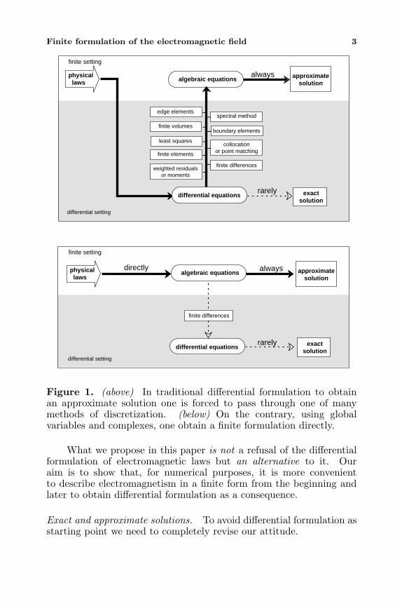
When applied to field theories, numerical methods require thesolution of a system of algebraic equations. It is standard practice toderive these equations starting from the differential equations resortingone of many discretization methods. This is the case, for instance,of finite difference methods, finite element methods, edge elementmethods, etc. This is summarized in the upper part of Fig. 1.
Even when an integral formulation is used, as in the finite volumemethod or in the finite integration theory (an extension of the finite-difference time-domain method), standard practice is to use integralsof field functions. Field functions are an indispensable ingredient ofdifferential formulation. At this point, one can pose the followingquestion: is it possible to express the laws of electromagnetism directlyby a set of algebraic equations, instead of obtaining them from adiscretization process applied to differential equations?
In this paper, we show that such a finite formulation is possible,it is simple, and that it is useful for numerical computation.
In such formulation, the classical procedure of writing the lawsof physics in differential form is inverted. Instead, we start fromfinite formulation and deduce differential formulation whenever it isrequired. In traditional methods, one is forced to select one of manydiscretization procedures. This is not the case of the finite formulationas illustrated in the lower part of Fig. 1.
Finite formulation of the electromagnetic field 3
finite setting
differential setting
rarely
finite setting
differential setting
always
always
rarely
finite differences
finite differences
spectral methodedge elements
finite volumes
least squares
finite elements
collocationor point matching
boundary elements
approximatesolution
algebraic equations
directly
exactsolution
exactsolution
differential equations
differential equations
algebraic equationsphysical laws
physical laws
approximatesolution
weighted residualsor moments
Figure 1. (above) In traditional differential formulation to obtainan approximate solution one is forced to pass through one of manymethods of discretization. (below) On the contrary, using globalvariables and complexes, one obtain a finite formulation directly.
What we propose in this paper is not a refusal of the differentialformulation of electromagnetic laws but an alternative to it. Ouraim is to show that, for numerical purposes, it is more convenientto describe electromagnetism in a finite form from the beginning andlater to obtain differential formulation as a consequence.
Exact and approximate solutions. To avoid differential formulation asstarting point we need to completely revise our attitude.
4 Tonti
In the paradigm formed by three centuries of differentialformulation of physical laws, we find the differential formulation soprevalent that we are led to think that it is the natural formulationfor physics. Moreover, we are convinced that differential formulationleads to an exact solution to physical problems.
However, we know full well that only in a few elementary caseswe can obtain a solution in closed form: hence the “exact solution”promised by differential formulation, is almost never attained inpractice. Moreover the great scientific and technological advancementobtained in our days by numerical solution of physical problems that donot admit a solution in closed form, suggests that this progress arisesmainly because we have found the way to obtain approximate solutionsto our problems. In our culture, modelled on mathematical analysis,the term “approximate” sounds flawed. Nevertheless the goal of anumerical simulation is agreement with experimental measurements.
To reduce error of an approximate solution does not mean to makethe error as small as we like, as a limit process requires, but to makeerror smaller than a preassigned tolerance.
We are well aware that all measurements are affected by atolerance: every measuring instrument belongs to a given class ofprecision. In measurements an “infinite” precision, in the sense of alimit process of mathematics, is not attainable. The same positioningof the measuring probe in a field implies a tolerance.
The notion of precision in measuring apparatus plays the samerole of the notion of tolerance in manufacturing and of the notion oferror in numerical analysis.
In conclusion one cannot deny the satisfaction of knowing theexact solution of a physical problem when the latter is available. Whatwe deny is the need to refer to an idealized exact solution when this isnot available in order to compare a numerical result with experience.
2. FINITE FORMULATION: THE PREMISES
A reformulation of field laws in a direct finite formulation must startwith an analysis of physical quantities in order to make explicit themaximum of information content that is implicit in definition and inmeasurement of physical quantities. To this end it is convenient tointroduce two classifications of physical quantities.
2.1. Configuration, Source and Energy Variables
A first classification criterion of great usefulness in teaching and inresearch is that based on the role that every physical variable plays in
Finite formulation of the electromagnetic field 5
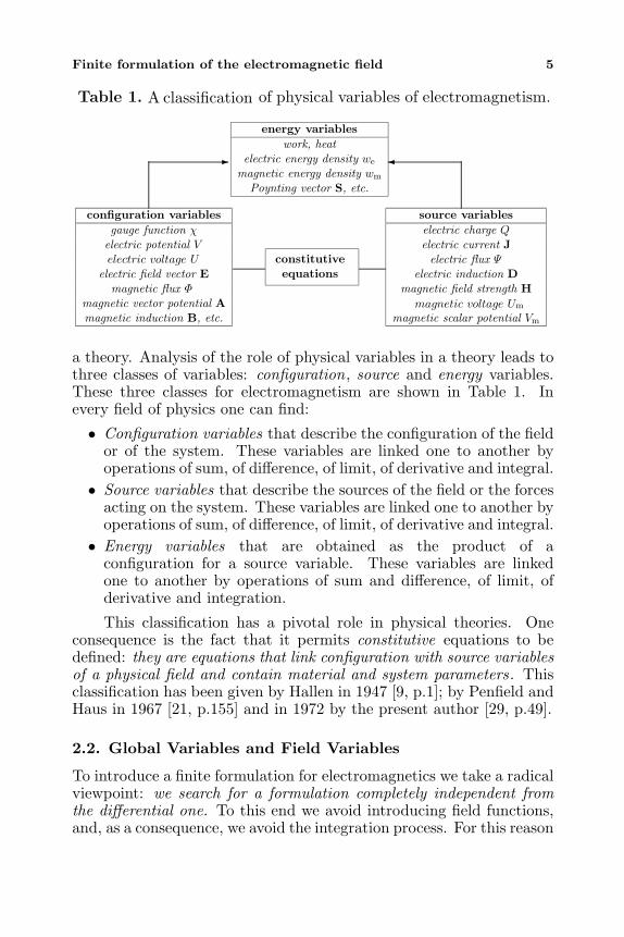
Table 1. A classification of physical variables of electromagnetism.
configuration variablesgauge function χ
electric potential Velectric voltage U
electric field vector Emagnetic flux Φ
magnetic vector potential Amagnetic induction B, etc.
constitutiveequations
source variableselectric charge Qelectric current Jelectric flux Ψ
electric induction Dmagnetic field strength H
magnetic scalar potential Vm
energy variableswork, heat
electric energy density we
magnetic energy density wm
Poynting vector S, etc.
magnetic voltage Um
a theory. Analysis of the role of physical variables in a theory leads tothree classes of variables: configuration, source and energy variables.These three classes for electromagnetism are shown in Table 1. Inevery field of physics one can find:
• Configuration variables that describe the configuration of the fieldor of the system. These variables are linked one to another byoperations of sum, of difference, of limit, of derivative and integral.• Source variables that describe the sources of the field or the forces
acting on the system. These variables are linked one to another byoperations of sum, of difference, of limit, of derivative and integral.
• Energy variables that are obtained as the product of aconfiguration for a source variable. These variables are linkedone to another by operations of sum and difference, of limit, ofderivative and integration.
This classification has a pivotal role in physical theories. Oneconsequence is the fact that it permits constitutive equations to bedefined: they are equations that link configuration with source variablesof a physical field and contain material and system parameters. Thisclassification has been given by Hallen in 1947 [9, p.1]; by Penfield andHaus in 1967 [21, p.155] and in 1972 by the present author [29, p.49].
2.2. Global Variables and Field Variables
To introduce a finite formulation for electromagnetics we take a radicalviewpoint: we search for a formulation completely independent fromthe differential one. To this end we avoid introducing field functions,and, as a consequence, we avoid the integration process. For this reason
6 Tonti
instead of the term “integral” quantity we shall use the equivalent termglobal quantity.
We must emphasize that physical measurements deal mainly withglobal variables, not with field variables. Field variables are needed in adifferential formulation because the very notion of derivative refers to apoint function. On the contrary a global quantity refers to a system, toa space or time element like a line, a surface, a volume, an interval, i.e.is a domain function. Thus a flow meter measures the electric chargethat crosses a given surface in a given time interval. A flux metermeasures the flux (=flow rate) associated with a surface at given timeinstant. The corresponding physical quantities are associated withspace and time elements, not only with points and instants.
One fundamental advantage of global variables is that they arecontinuous through the separation surface of two materials while thefield variables suffer discontinuity. This implies that the differentialformulation is restricted to regions of material homogeneity: one mustbreak the domain in subdomains, one for every material and introducejump conditions. If one reflects on the great number of differentmaterials present in a real device, one can see that the idealizationrequired by differential formulation is too restrictive.
This shows that differential formulation imposes differentiabilityconditions on field functions that are restrictive from the physical pointof view .
Contrary to this, a direct finite formulation based on globalvariables accepts material discontinuities, i.e. does not add regularityconditions to those requested by the physical nature of the variable.
To help the reader, accustomed to thinking in terms of traditionalfield variables ρ,J,B,D,E,H, we first examine corresponding integralvariables Qc, Qf ,Φ,Ψ ,U ,Um: these are collected in Table 2. This tableshows that integral variables arise by integration of field functions onspace domains i.e. lines, surfaces, volumes and on time intervals. Thetime integral of a physical variable, say F , will be called its impulse andwill be denoted by the corresponding calligraphic letter, say F . Thelast three variables of the left side, K, G, Λ deals with the hypotheticalmagnetic monopole charge, monopole flow, monopole production. Therole of these variables and of the corresponding ones τ,Vm, η of theright side is clarified in Table 2.
It is remarkable that the integral configuration variables all havethe dimension of a magnetic flux and that integral source variables allhave the dimension of a charge. The product of a global configurationvariable and a global source variable has the dimension of an action(energy× time).
Table 3 shows the six integral variables that are measurable and
Finite formulation of the electromagnetic field 7
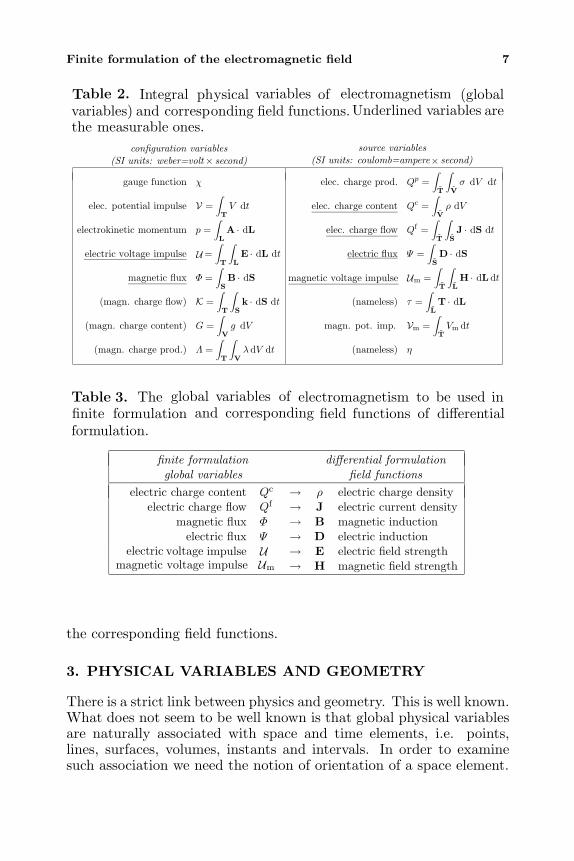
Table 2. Integral physical variables of electromagnetism (globalvariables) and corresponding field functions.Underlined variables arethe measurable ones.
configuration variables source variables(SI units: weber=volt× second) (SI units: coulomb=ampere× second)
gauge function χ elec. charge prod. Qp =∫T
∫V
σ dV dt
elec. potential impulse V =∫T
V dt elec. charge content Qc =∫V
ρ dV
electrokinetic momentum p =∫LA · dL elec. charge flow Qf =
∫T
∫SJ · dS dt
impulse =∫T
∫LE · dL dt electric flux Ψ =
∫SD · dS
magnetic flux Φ =∫SB · dS impulse m =
∫T
∫LH · dLdt
(magn. charge flow) K =∫T
∫Sk · dS dt (nameless) τ =
∫LT · dL
(magn. charge content) G =∫V
g dV magn. pot. imp. Vm =∫T
Vm dt
(magn. charge prod.) Λ =∫T
∫V
λ dV dt (nameless) η
Table The global variables of electromagnetism to be used infinite formulation and corresponding field functions of differentialformulation.
finite formulation differential formulationglobal variables field functions
electric charge content Qc → ρ electric charge densityelectric charge flow Qf → J electric current density
magnetic flux Φ → B magnetic inductionelectric flux Ψ → D electric induction
impulse → E electric field strength→ H magnetic field strength
3.
voltage U
magnetic voltage U
voltage Uimpulse mmagnetic voltage U
electric
electric
the corresponding field functions.
3. PHYSICAL VARIABLES AND GEOMETRY
There is a strict link between physics and geometry. This is well known.What does not seem to be well known is that global physical variablesare naturally associated with space and time elements, i.e. points,lines, surfaces, volumes, instants and intervals. In order to examinesuch association we need the notion of orientation of a space element.
8 Tonti
In differential formulation a fundamental role is played by points:field functions are point functions. In order to associate points withnumbers we introduce coordinate systems.
In finite formulation we need to consider not only points (P) butalso lines (L), surfaces (S) and volumes (V). We shall call thesespace elements. We use a boldface characters for reasons that willbe explained later. The natural substitute of coordinate systems arecell complexes. They exhibit vertices, edges, faces and cells. The latterare representative of the four spatial elements P,L,S,V.
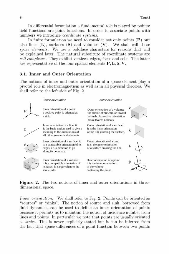
3.1. Inner and Outer Orientation
The notions of inner and outer orientation of a space element play apivotal role in electromagnetism as well as in all physical theories. Weshall refer to the left side of Fig. 2.
Inner orientation of a line: itis the basic notion used to give a meaning to the orientations of all other geometrical elements.
Inner orientation of a surface: itis a compatible orientation of its edges, i.e. a direction to go along its boundary.
Inner orientation of a volume:it is a compatible orientation of its faces. It is equivalent to the screw rule.
Outer orientation of a volume:the choice of outward or inward normals. A positive orientationhas outwards normals.
Outer orientation of a surface:it is the inner orientation of the line crossing the surface.
Outer orientation of a line:it is the inner orientationof a surface crossing the line.
Outer orientation of a point: it is the inner orientation of the volume containing the point.
Inner orientation of a point:a positive point is oriented asa sink.
outer orientation inner orientation
P
L
S
V
P
L
S
V
Figure 2. The two notions of inner and outer orientations in three-dimensional space.
Inner orientation. We shall refer to Fig. 2. Points can be oriented as“sources” or “sinks”. The notion of source and sink, borrowed fromfluid dynamics, can be used to define an inner orientation of pointsbecause it permits us to maintain the notion of incidence number fromlines and points. In particular we note that points are usually orientedas sinks. This is never explicitly stated but it can be inferred fromthe fact that space differences of a point function between two points
Finite formulation of the electromagnetic field 9
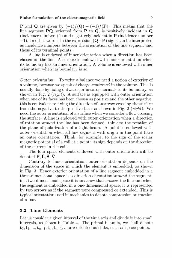
P and Q are given by (+1)f(Q) + (−1)f(P). This means that theline segment PQ, oriented from P to Q, is positively incident in Q(incidence number +1) and negatively incident in P (incidence number−1). In other words: in the expression (Q−P) signs can be interpretedas incidence numbers between the orientation of the line segment andthose of its terminal points.
A line is endowed of inner orientation when a direction has beenchosen on the line. A surface is endowed with inner orientation whenits boundary has an inner orientation. A volume is endowed with innerorientation when its boundary is so.
Outer orientation. To write a balance we need a notion of exterior ofa volume, because we speak of charge contained in the volume. This isusually done by fixing outwards or inwards normals to its boundary, asshown in Fig. 2 (right). A surface is equipped with outer orientationwhen one of its faces has been chosen as positive and the other negative:this is equivalent to fixing the direction of an arrow crossing the surfacefrom the negative to the positive face, as shown in Fig. 2 (right). Weneed the outer orientation of a surface when we consider a flow crossingthe surface. A line is endowed with outer orientation when a directionof rotation around the line has been defined: think to the rotation ofthe plane of polarization of a light beam. A point is endowed withouter orientation when all line segment with origin in the point havean outer orientation. Think, for example, to the sign of the scalarmagnetic potential of a coil at a point: its sign depends on the directionof the current in the coil.
The four space elements endowed with outer orientation will bedenoted P, L, S, V.
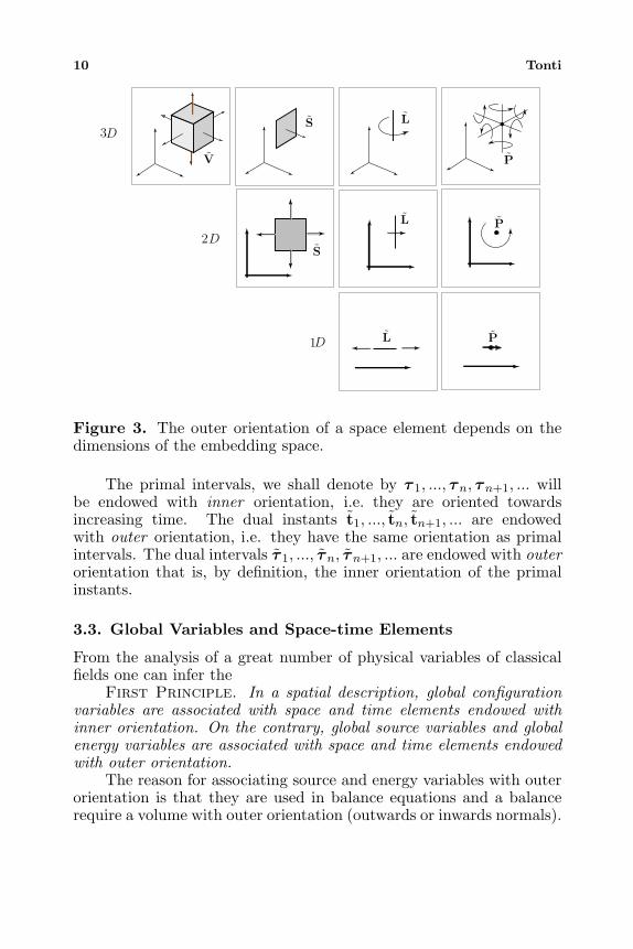
Contrary to inner orientation, outer orientation depends on thedimension of the space in which the element is embedded, as shownin Fig. 3. Hence exterior orientation of a line segment embedded in athree-dimensional space is a direction of rotation around the segment;in a two-dimensional space it is an arrow that crosses the line and whenthe segment is embedded in a one-dimensional space, it is representedby two arrows as if the segment were compressed or extended. This istypical orientation used in mechanics to denote compression or tractionof a bar.
3.2. Time Elements
Let us consider a given interval of the time axis and divide it into smallintervals, as shown in Table 4. The primal instants, we shall denotet0, t1, ..., tn−1, tn, tn+1, ... are oriented as sinks, such as space points.
10 Tonti
1
2
3D
D
D
V
S
S
L
L
L
P
P
P
Figure 3. The outer orientation of a space element depends on thedimensions of the embedding space.
The primal intervals, we shall denote by τ 1, ..., τn, τn+1, ... willbe endowed with inner orientation, i.e. they are oriented towardsincreasing time. The dual instants t1, ..., tn, tn+1, ... are endowedwith outer orientation, i.e. they have the same orientation as primalintervals. The dual intervals τ 1, ..., τn, τn+1, ... are endowed with outerorientation that is, by definition, the inner orientation of the primalinstants.
3.3. Global Variables and Space-time Elements
From the analysis of a great number of physical variables of classicalfields one can infer the
First Principle. In a spatial description, global configurationvariables are associated with space and time elements endowed withinner orientation. On the contrary, global source variables and globalenergy variables are associated with space and time elements endowedwith outer orientation.
The reason for associating source and energy variables with outerorientation is that they are used in balance equations and a balancerequire a volume with outer orientation (outwards or inwards normals).
Finite formulation of the electromagnetic field 11
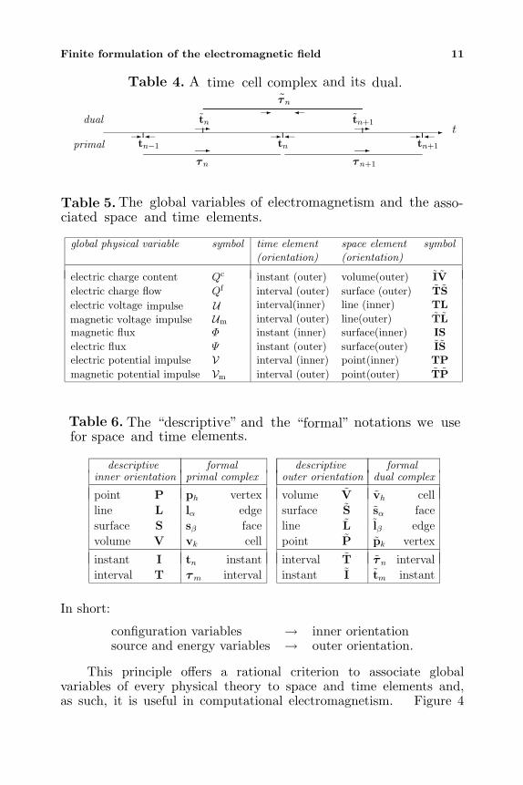
Table A time cell complex and its dual.
tprimal
tn−1 tn tn+1
τn τn+1
dual tn tn+1
τn
Table The global variables of electromagnetism and the asso-ciated space and time elements.
global physical variable symbol time element space element symbol(orientation) (orientation)
electric charge content Qc instant (outer) volume(outer) IVelectric charge flow Qf interval (outer) surface (outer) TS
impulse interval(inner) line (inner) TLimpulse m interval (outer) line(outer) TL
magnetic flux Φ instant (inner) surface(inner) ISelectric flux Ψ instant (outer) surface(outer) ISelectric potential impulse V interval (inner) point(inner) TPmagnetic potential impulse Vm interval (outer) point(outer) TP
Table The “descriptive” and the “formal” notations we usefor space and time elements.
descriptive formal descriptive formalinner orientation primal complex outer orientation dual complex
point P ph vertex volume V vh cell
line L lα edge surface S sα face
surface S sβ face line L lβ edge
volume V vk cell point P pk vertex
instant I tn instant interval T τ n interval
interval T τm interval instant I tm instant
4.
5.
6.
UU
electric voltagemagnetic voltage
In short:
configuration variables → inner orientationsource and energy variables → outer orientation.
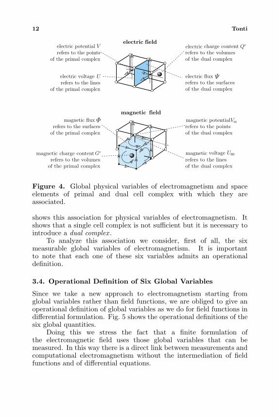
This principle offers a rational criterion to associate globalvariables of every physical theory to space and time elements and,as such, it is useful in computational electromagnetism. Figure 4
12 Tonti
electric field
magnetic fieldmagnetic flux
refers to the surfacesof the primal complex
electric fluxrefers to the surfacesof the dual complex
electric potentialrefers to the points
of the primal complex
V
refers to the linesof the primal complex
magnetic charge contentrefers to the volumes
of the primal complex
Gc
electric charge contentrefers to the volumesof the dual complex
Qc
magnetic potentialrefers to the pointsof the dual complex
Vm
refers to the linesof the dual complex
Φ
Ψ
m
electric voltage U
Umagnetic voltage
Figure 4. Global physical variables of electromagnetism and spaceelements of primal and dual cell complex with which they areassociated.
shows this association for physical variables of electromagnetism. Itshows that a single cell complex is not sufficient but it is necessary tointroduce a dual complex .
To analyze this association we consider, first of all, the sixmeasurable global variables of electromagnetism. It is importantto note that each one of these six variables admits an operationaldefinition.
3.4. Operational Definition of Six Global Variables
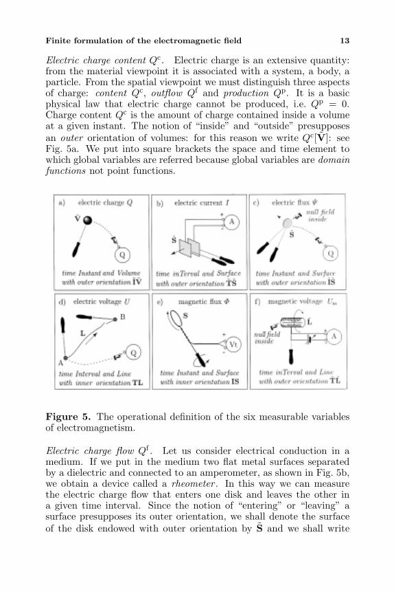
Since we take a new approach to electromagnetism starting fromglobal variables rather than field functions, we are obliged to give anoperational definition of global variables as we do for field functions indifferential formulation. Fig. 5 shows the operational definitions of thesix global quantities.
Doing this we stress the fact that a finite formulation ofthe electromagnetic field uses those global variables that can bemeasured. In this way there is a direct link between measurements andcomputational electromagnetism without the intermediation of fieldfunctions and of differential equations.
Finite formulation of the electromagnetic field 13
Electric charge content Qc. Electric charge is an extensive quantity:from the material viewpoint it is associated with a system, a body, aparticle. From the spatial viewpoint we must distinguish three aspectsof charge: content Qc, outflow Qf and production Qp. It is a basicphysical law that electric charge cannot be produced, i.e. Qp = 0.Charge content Qc is the amount of charge contained inside a volumeat a given instant. The notion of “inside” and “outside” presupposesan outer orientation of volumes: for this reason we write Qc[V]: seeFig. 5a. We put into square brackets the space and time element towhich global variables are referred because global variables are domainfunctions not point functions.
Figure 5. The operational definition of the six measurable variablesof electromagnetism.
Electric charge flow Qf . Let us consider electrical conduction in amedium. If we put in the medium two flat metal surfaces separatedby a dielectric and connected to an amperometer, as shown in Fig. 5b,we obtain a device called a rheometer . In this way we can measurethe electric charge flow that enters one disk and leaves the other ina given time interval. Since the notion of “entering” or “leaving” asurface presupposes its outer orientation, we shall denote the surfaceof the disk endowed with outer orientation by S and we shall write
14 Tonti
Qf [S]. The rate of this quantity is the electric current I.
Electric flux Ψ. Let us consider an electrostatic field. If we puta small metal disk somewhere in the field then charges of oppositesign will be collected on the two faces as a consequence of electricalinduction. After selection of one face as positive we call electric fluxΨ the charge collected on this positive face of the disk. The electricflux is then related to an outer oriented surface. If we change the outerorientation of the surface, the sign of the flux changes. As we see fromthis definition, electric flux requires the notion of the outer orientationof a surface and hence we shall write Ψ [S].
To measure electric flux, instead of one metal disk, it is betterto use two small metal disks. The disks will be held by an insulatedhandle and brought into contact, as shown in Fig. 5c. If we separate thetwo disks also the electric charges will be separated and each one canbe measured with an electrometer. The charge collected on a prefixeddisk is, by definition, electric flux (this direct measurement of electricflux is often ignored in books of electromagnetism. It can be found inMaxwell [18, p.47] and in [8, p.71]; [7, p.61]; [25, p.230]; [26, p.25]; [12,p.80; p.225]).
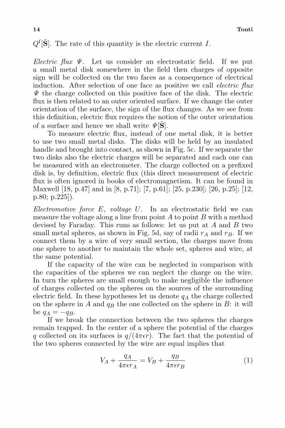
Electromotive force E, voltage U . In an electrostatic field we canmeasure the voltage along a line from point A to point B with a methoddevised by Faraday. This runs as follows: let us put at A and B twosmall metal spheres, as shown in Fig. 5d, say of radii rA and rB. If weconnect them by a wire of very small section, the charges move fromone sphere to another to maintain the whole set, spheres and wire, atthe same potential.
If the capacity of the wire can be neglected in comparison withthe capacities of the spheres we can neglect the charge on the wire.In turn the spheres are small enough to make negligible the influenceof charges collected on the spheres on the sources of the surroundingelectric field. In these hypotheses let us denote qA the charge collectedon the sphere in A and qB the one collected on the sphere in B: it willbe qA = −qB.
If we break the connection between the two spheres the chargesremain trapped. In the center of a sphere the potential of the chargesq collected on its surfaces is q/(4πεr). The fact that the potential ofthe two spheres connected by the wire are equal implies that
VA +qA
4πεrA= VB +
qB4πεrB
(1)
Finite formulation of the electromagnetic field 15
from which we obtain
VAB ≡ VB − VA =−qA4πε
(1rA
+1rB
). (2)
Hence we can measure voltage from measuring the charge collected onone sphere.
In particular if we choose B on the grounds the “sphere” Bbecomes the Earth and then VB = 0 and 1/rB = 0: it follows [22,p.519]
VA =−qA
4πεrA. (3)
The voltage refers to a line endowed with inner orientation: V [L] asshown in Fig. 5d.
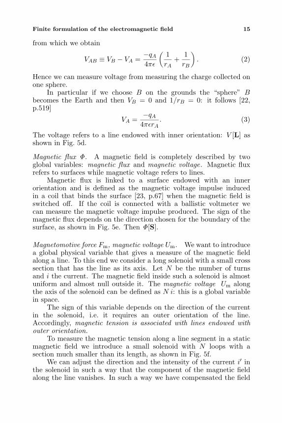
Magnetic flux Φ. A magnetic field is completely described by twoglobal variables: magnetic flux and magnetic voltage. Magnetic fluxrefers to surfaces while magnetic voltage refers to lines.
Magnetic flux is linked to a surface endowed with an innerorientation and is defined as the magnetic voltage impulse inducedin a coil that binds the surface [23, p.67] when the magnetic field isswitched off. If the coil is connected with a ballistic voltmeter wecan measure the magnetic voltage impulse produced. The sign of themagnetic flux depends on the direction chosen for the boundary of thesurface, as shown in Fig. 5e. Then Φ[S].
Magnetomotive force Fm, magnetic voltage Um. We want to introducea global physical variable that gives a measure of the magnetic fieldalong a line. To this end we consider a long solenoid with a small crosssection that has the line as its axis. Let N be the number of turnsand i the current. The magnetic field inside such a solenoid is almostuniform and almost null outside it. The magnetic voltage Um alongthe axis of the solenoid can be defined as N i: this is a global variablein space.
The sign of this variable depends on the direction of the currentin the solenoid, i.e. it requires an outer orientation of the line.Accordingly, magnetic tension is associated with lines endowed withouter orientation.
To measure the magnetic tension along a line segment in a staticmagnetic field we introduce a small solenoid with N loops with asection much smaller than its length, as shown in Fig. 5f.
We can adjust the direction and the intensity of the current i′ inthe solenoid in such a way that the component of the magnetic fieldalong the line vanishes. In such a way we have compensated the field
16 Tonti
in the interior region. Let us put I ′ = N i′: the magnetomotive forcealong the line is then Fm = −I ′. This procedure is known as themethod of compensating coil [8, p.224]; [23, p.66]; [26, p.41].
This shows that magnetic tension is associated with a line withthe direction of rotation around it: the direction is opposite to the oneof the compensating current. Denoting by L a line segment endowedwith an outer orientation we can write
Um[L] def= −I ′. (4)
An equivalent way to do the test is to consider a small tube ofsuperconducting material: the tube will be crossed by a uniformcurrent I ′ that automatically makes the interior field vanish [16, p.494].
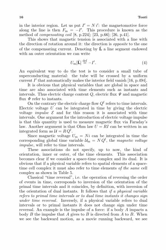
It is obvious that physical variables that are global in space andtime are also associated with time elements such as instants andintervals. Thus electric charge content Q, electric flux Ψ and magneticflux Φ refer to instants.
On the contrary the electric charge flow Qf refers to time intervals.Electric voltage U can be integrated in time by giving the electricvoltage impulse E and for this reason it is associated with timeintervals. One argument for the introduction of electric voltage impulseis that this quantity is used to measure magnetic flux via Faraday’slaw. Another argument is that Ohm law U = RI can be written in anintegrated form as U = R Qf .
Since magnetic voltage Um = Ni can be integrated in time thecorresponding global time variable Um = N Qf , the magnetic voltageimpulse, will refer to time intervals.
These associations do not specify, up to now, the kind oforientation, inner or outer, of the time elements. This associationbecomes clear if we consider a space-time complex and its dual. It isobvious that if a physical variable refers to spatial elements of a space-time cell complex it must also refer to time elements of the same cellcomplex as shown in Table 5.
Classical “time reversal”, i.e. the operation of reversing the orderof events in time, corresponds to inversion of the orientation of theprimal time intervals and it coincides, by definition, with inversion ofthe orientation of dual instants. It follows that if a physical variablerefers to primal time intervals or to dual time instants it changes signunder time reversal . Inversely, if a physical variable refers to dualintervals or to primal instants it does not change sign under timereversal. An example is the impulse of a force: if a body A impacts abody B the impulse that A gives to B is directed from A to B. Whenwe see the backward motion, as a movie running backward, we see
Finite formulation of the electromagnetic field 17
x
y
x
y
z
tim
e
Φ
space
V
V
Φ
ΦΦ
space
a) b)
Qc
Ψ, Qf
Ψ, Qf
Ψ, Qf
Ψ, Qc
E,U
U
V
V
E,U
Fm
m
, Qf
Fm m, ,Qf
Fm
E,U
E,U
Figure 6. a) A space complex and associated variables; b) a three-dimensional space-time and associated variables.
that velocities are inverted but the impulse that A gives to B is alwaysdirected from A to B.
The space and time association of global electromagnetic variablesis summarized in Table 5.
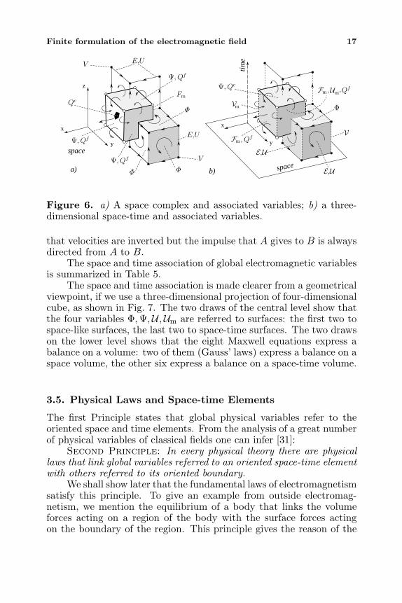
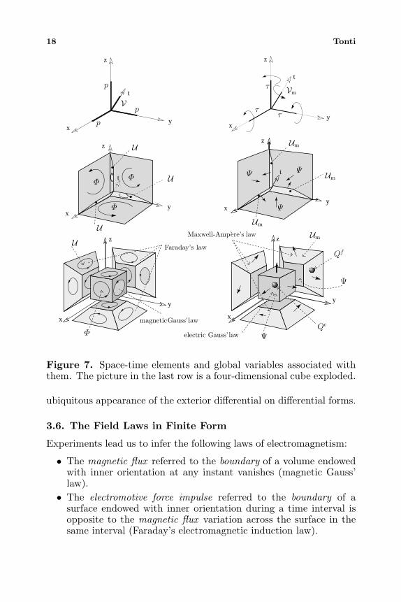
The space and time association is made clearer from a geometricalviewpoint, if we use a three-dimensional projection of four-dimensionalcube, as shown in Fig. 7. The two draws of the central level show thatthe four variables Φ,Ψ,U ,Um are referred to surfaces: the first two tospace-like surfaces, the last two to space-time surfaces. The two drawson the lower level shows that the eight Maxwell equations express abalance on a volume: two of them (Gauss’ laws) express a balance on aspace volume, the other six express a balance on a space-time volume.
3.5. Physical Laws and Space-time Elements
The first Principle states that global physical variables refer to theoriented space and time elements. From the analysis of a great numberof physical variables of classical fields one can infer [31]:
Second Principle: In every physical theory there are physicallaws that link global variables referred to an oriented space-time elementwith others referred to its oriented boundary.
We shall show later that the fundamental laws of electromagnetismsatisfy this principle. To give an example from outside electromag-netism, we mention the equilibrium of a body that links the volumeforces acting on a region of the body with the surface forces actingon the boundary of the region. This principle gives the reason of the
18 Tonti
z
t
yx
z
t
yx
t
y
y
x
x
z
t
y
y
x
x
z
z z
Φ
Φ
Φ
Φ
Ψ
Ψ Ψ
Gauss’law
electric Gauss’law
Faraday’s law
Maxwell-Ampere’s law
magnetic
p
p
p
Qc
Qf
Ψ
Ψ
U
U
UU
V
Um
Um
Um
Um
Vm
ττ
τ
Figure 7. Space-time elements and global variables associated withthem. The picture in the last row is a four-dimensional cube exploded.
ubiquitous appearance of the exterior differential on differential forms.
3.6. The Field Laws in Finite Form
Experiments lead us to infer the following laws of electromagnetism:
• The magnetic flux referred to the boundary of a volume endowedwith inner orientation at any instant vanishes (magnetic Gauss’law).
• The electromotive force impulse referred to the boundary of asurface endowed with inner orientation during a time interval isopposite to the magnetic flux variation across the surface in thesame interval (Faraday’s electromagnetic induction law).
Finite formulation of the electromagnetic field 19
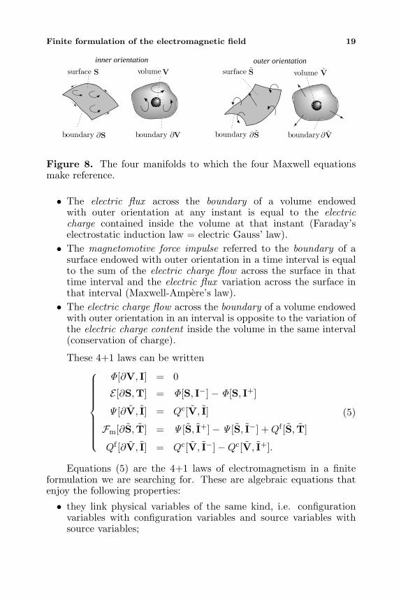
vouter orientationinner orientation
boundary ∂S
surface S
boundary ∂V
olumeV
boundary ∂S
surface S
boundary∂V
volume V
Figure 8. The four manifolds to which the four Maxwell equationsmake reference.
• The electric flux across the boundary of a volume endowedwith outer orientation at any instant is equal to the electriccharge contained inside the volume at that instant (Faraday’selectrostatic induction law = electric Gauss’ law).
• The magnetomotive force impulse referred to the boundary of asurface endowed with outer orientation in a time interval is equalto the sum of the electric charge flow across the surface in thattime interval and the electric flux variation across the surface inthat interval (Maxwell-Ampere’s law).• The electric charge flow across the boundary of a volume endowed
with outer orientation in an interval is opposite to the variation ofthe electric charge content inside the volume in the same interval(conservation of charge).
These 4+1 laws can be written
Φ[∂V, I] = 0
E [∂S,T] = Φ[S, I−]− Φ[S, I+]
Ψ [∂V, I] = Qc[V, I]
Fm[∂S, T] = Ψ [S, I+]−Ψ [S, I−] + Qf [S, T]
Qf [∂V, I] = Qc[V, I−]−Qc[V, I+].
(5)
Equations (5) are the 4+1 laws of electromagnetism in a finiteformulation we are searching for. These are algebraic equations thatenjoy the following properties:
• they link physical variables of the same kind, i.e. configurationvariables with configuration variables and source variables withsource variables;
20 Tonti
• they are valid in whatever medium and then are free from anymaterial parameter;
• they do not involve metrical notions, i.e. lengths, areas, measuresof volumes and durations are not required [37].
These five equations, that are equivalent to the integral formulationdescribe the “structure” of the field and we shall call them equationof structure. Since they are valid for whatever volume and whateversurface respectively they are of topological nature and we can namethem also topological equations [20, p.20] [36].
4. CELL COMPLEXES IN SPACE AND TIME
The equations (5) are the finite formulation of the electromagneticlaws. How to apply them to solve field problems? The principle is avery simple one: we build up a cell complex in the region in whichthe field is considered and then apply the equations in finite form toall cells of the complex. Some equations must be applied to the cellsothers to their faces; some equations must be applied to the cells andfaces of the primal, some other to those of the dual complex. Doingso we obtain a system of algebraic equations whose solution gives thespace and time distribution of the global variables of the field. In thisway we solve the fundamental problem of electromagnetism: given thespace and time distribution of charges and currents to find the resultingfield .
To pursue this goal we must introduce the notion of cell complexand of its dual. Let us consider, first of all, a cell complex formed bycubic cells, as shown in Fig. 9c.
The elements of the same dimension can be numbered accordingto any criterion. The number is a label that permits us to specifythe space element and play the same role of coordinates of a point ina coordinate system. We shall consider cell complexes with a finitenumber N0 of vertices. Since vertices are points we shall denote thetypical vertex by ph. At first it seems convenient to assign to everyedge a pair of numbers, the labels of its bounding points. Thus theedge that connects the vertex ph with the vertex pk can be denotedlhk. But this notation becomes cumbersome so that we have chosen todenote the edge with a single Greek index, e.g. lα. If N1 is the numberof edges the Greek index takes the values 1, 2, ...N1. We shall denotewith a Greek index also the face, e.g. sβ while the typical cell will bedenoted with a Latin index, e.g. vk.
As in space we have four elements, so in time we have two elements:instants I and intervals T. When we consider a cell complex on the timeaxis we shall denote by tn the time instants and τm the intervals.
Finite formulation of the electromagnetic field 21
x
y
z
x
y
time
space
t
time
time
x
t
a
f
d
e
x
x
c
b
y
L L
LL L
P P P
P P P
P
P
P
L
SS
S
S
V
I I I
T T
P
P
L
L
L
S
S
S
VI I I
T T
IP
IP
TP
TP
IL
IL
IL
TL
TL
IS
TS
IS
TP
TL
IP
TS
TS
IL
TL
IP
IL
TP
P PP
PPP
L L
T
I
I
I
I
T
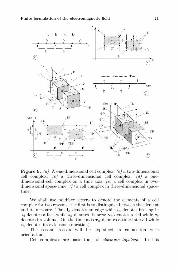
Figure 9. (a) A one-dimensional cell complex; (b) a two-dimensionalcell complex; (c) a three-dimensional cell complex; (d) a one-dimensional cell complex on a time axis; (e) a cell complex in two-dimensional space-time; (f) a cell complex in three-dimensional space-time.
We shall use boldface letters to denote the elements of a cellcomplex for two reasons: the first is to distinguish between the elementand its measure. Thus lα denotes an edge while lα denotes its length;sβ denotes a face while sβ denotes its area; vk denotes a cell while vkdenotes its volume. On the time axis τn denotes a time interval whileτn denotes its extension (duration).
The second reason will be explained in connection withorientation.
Cell complexes are basic tools of algebraic topology . In this
22 Tonti
branch of topology many notions were developed around cell complexesincluding the notions of orientation, duality and incidence numbers. Inalgebraic topology vertices, edges and faces of cells are considered ascells of a lower dimension. The vertices are called 0-dimensional cellsor briefly 0-cells, edges 1-cells, faces 2-cells and original cells 3-cells.It follows that a cell complex in space is not only a set of 3-cells but aset of p -cells with p = 0, 1, 2, 3. In four-dimensional space-time a cellcomplex is formed by cells of dimension p = 0, 1, 2, 3, 4.
Table 6 (left) collects the notations we use for space elements:when we must mention points, lines, surfaces and volumes withoutreference to a cell complex we shall use a “descriptive” notation withboldface, uppercase letters. On the contrary, when we refer to acell complex we must specify the labels of the elements involved andaccordingly we shall use a “formal” notation with boldface, lowercaseletters with indices.
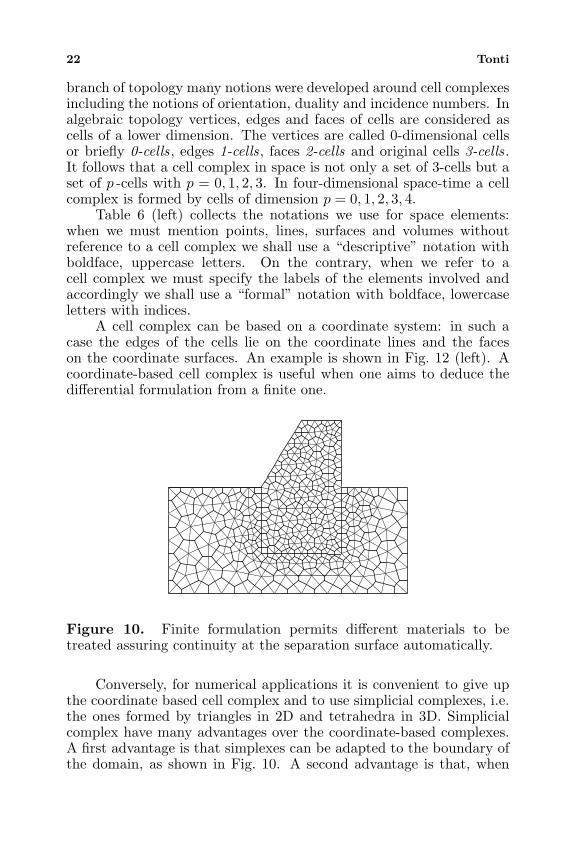
A cell complex can be based on a coordinate system: in such acase the edges of the cells lie on the coordinate lines and the faceson the coordinate surfaces. An example is shown in Fig. 12 (left). Acoordinate-based cell complex is useful when one aims to deduce thedifferential formulation from a finite one.
Figure 10. Finite formulation permits different materials to betreated assuring continuity at the separation surface automatically.
Conversely, for numerical applications it is convenient to give upthe coordinate based cell complex and to use simplicial complexes, i.e.the ones formed by triangles in 2D and tetrahedra in 3D. Simplicialcomplex have many advantages over the coordinate-based complexes.A first advantage is that simplexes can be adapted to the boundary ofthe domain, as shown in Fig. 10. A second advantage is that, when
Finite formulation of the electromagnetic field 23
we have two or more subregions that contain different materials, thevertices of the simplexes can be put on the separation surface, as shownin Fig. 10. A third reason is that simplexes can change in size fromone region to another. This allows to adopt smaller simplexes in theregions of large variations of the field.
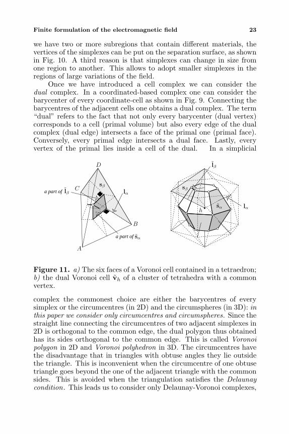
Once we have introduced a cell complex we can consider thedual complex. In a coordinated-based complex one can consider thebarycenter of every coordinate-cell as shown in Fig. 9. Connecting thebarycentres of the adjacent cells one obtains a dual complex. The term“dual” refers to the fact that not only every barycenter (dual vertex)corresponds to a cell (primal volume) but also every edge of the dualcomplex (dual edge) intersects a face of the primal one (primal face).Conversely, every primal edge intersects a dual face. Lastly, everyvertex of the primal lies inside a cell of the dual. In a simplicial
lα
lα
sα
sα
sβsβ
lβ
lβ
A
B
C
D
h
a part of
a part of
Figure 11. a) The six faces of a Voronoi cell contained in a tetraedron;b) the dual Voronoi cell vh of a cluster of tetrahedra with a commonvertex.
complex the commonest choice are either the barycentres of everysimplex or the circumcentres (in 2D) and the circumspheres (in 3D): inthis paper we consider only circumcentres and circumspheres. Since thestraight line connecting the circumcentres of two adjacent simplexes in2D is orthogonal to the common edge, the dual polygon thus obtainedhas its sides orthogonal to the common edge. This is called Voronoipolygon in 2D and Voronoi polyhedron in 3D. The circumcentres havethe disadvantage that in triangles with obtuse angles they lie outsidethe triangle. This is inconvenient when the circumcentre of one obtusetriangle goes beyond the one of the adjacent triangle with the commonsides. This is avoided when the triangulation satisfies the Delaunaycondition. This leads us to consider only Delaunay-Voronoi complexes,
24 Tonti
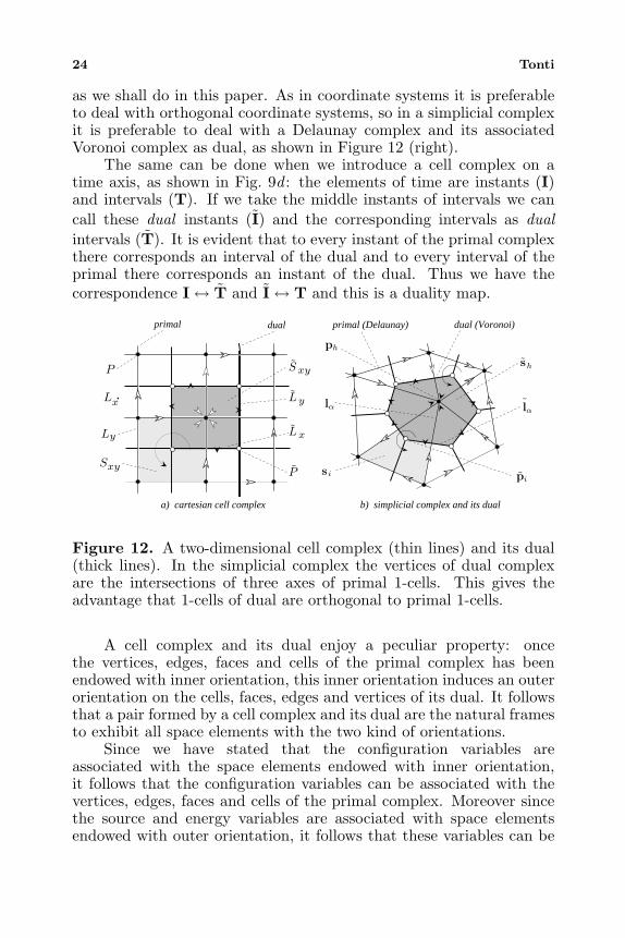
as we shall do in this paper. As in coordinate systems it is preferableto deal with orthogonal coordinate systems, so in a simplicial complexit is preferable to deal with a Delaunay complex and its associatedVoronoi complex as dual, as shown in Figure 12 (right).
The same can be done when we introduce a cell complex on atime axis, as shown in Fig. 9d : the elements of time are instants (I)and intervals (T). If we take the middle instants of intervals we cancall these dual instants (I) and the corresponding intervals as dualintervals (T). It is evident that to every instant of the primal complexthere corresponds an interval of the dual and to every interval of theprimal there corresponds an instant of the dual. Thus we have thecorrespondence I↔ T and I↔ T and this is a duality map.
dual (Voronoi)primal dual primal (Delaunay)
Lx
Ly
Sxy
P
P
Ly
Lx
Sxy
b) simplicial complex and its duala) cartesian cell complex
ph
h
lα lα
s pii ˜
s
˜
Figure 12. A two-dimensional cell complex (thin lines) and its dual(thick lines). In the simplicial complex the vertices of dual complexare the intersections of three axes of primal 1-cells. This gives theadvantage that 1-cells of dual are orthogonal to primal 1-cells.
A cell complex and its dual enjoy a peculiar property: oncethe vertices, edges, faces and cells of the primal complex has beenendowed with inner orientation, this inner orientation induces an outerorientation on the cells, faces, edges and vertices of its dual. It followsthat a pair formed by a cell complex and its dual are the natural framesto exhibit all space elements with the two kind of orientations.
Since we have stated that the configuration variables areassociated with the space elements endowed with inner orientation,it follows that the configuration variables can be associated with thevertices, edges, faces and cells of the primal complex. Moreover sincethe source and energy variables are associated with space elementsendowed with outer orientation, it follows that these variables can be
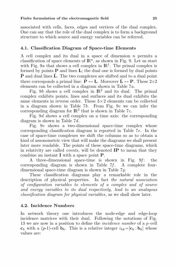
Finite formulation of the electromagnetic field 25
associated with cells, faces, edges and vertices of the dual complex.One can say that the role of the dual complex is to form a backgroundstructure to which source and energy variables can be referred.
4.1. Classification Diagram of Space-time Elements
A cell complex and its dual in a space of dimension n permits aclassification of space elements of IRn, as shown in Fig. 9. Let us startwith Fig. 9a that shows a cell complex in IR1. The primal complex isformed by points P and lines L; the dual one is formed by dual pointsP and dual lines L. The two complexes are shifted and to a dual pointthere corresponds a primal line: P↔ L. Moreover L↔ P. These 2×2elements can be collected in a diagram shown in Table 7a.
Fig. 9b shows a cell complex in IR2 and its dual. The primalcomplex exhibits points, lines and surfaces and its dual exhibits thesame elements in reverse order. These 3×2 elements can be collectedin a diagram shown in Table 7b. From Fig. 9c we can infer thecorresponding diagram for IR3 that is shown in Table 7c.
Fig. 9d shows a cell complex on a time axis: the correspondingdiagram is shown in Table 7d .
Fig. 9e shows a two-dimensional space-time complex whosecorresponding classification diagram is reported in Table 7e. In thecase of space-time complexes we shift the columns so as to obtain akind of assonometric view that will make the diagrams we shall presentlater more readable. The points of these space-time diagrams, whichin relativity are called events, will be denoted IP to mean that theycombine an instant I with a space point P.
A three-dimensional space-time is shown in Fig. 9f : thecorresponding diagram is shown in Table 7f . A complete four-dimensional space-time diagram is shown in Table 7g .
These classification diagrams play a remarkable role in thedescription of physical properties. In fact the natural associationof configuration variables to elements of a complex and of sourceand energy variables to its dual respectively, lead to an analogousclassification diagram for physical variables, as we shall show later.
4.2. Incidence Numbers
In network theory one introduces the node-edge and edge-loopincidence matrices with their dual. Following the notations of Fig.13 we are now in a position to define the incidence number of a p -cellch with a (p-1)-cell bk. This is a relative integer ihk=[ch : bk] whosevalues are:
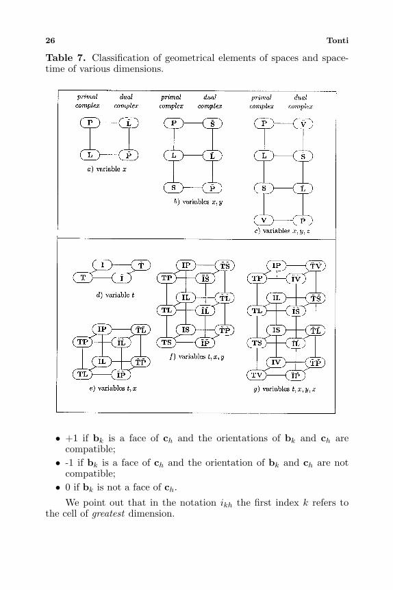
26 Tonti
Table 7. Classification of geometrical elements of spaces and space-time of various dimensions.
• +1 if bk is a face of ch and the orientations of bk and ch arecompatible;
• -1 if bk is a face of ch and the orientation of bk and ch are notcompatible;
• 0 if bk is not a face of ch.
We point out that in the notation ikh the first index k refers tothe cell of greatest dimension.
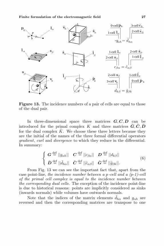
Finite formulation of the electromagnetic field 27
1-cell
0-cell 3-cell
2-cell
dkβ = gβk
1-cell
0-cell3-cell
2-cell
cβα = cαβ
1-cell
1-cell2-cell
2-cell
gαh= dhα-
ph
p
p
hlαlα
ll
l
αlα
sα
sα
sα
˜αsβ
s
s
β
sβ
sβ
βl
β˜
˜l
β˜
β
˜
vhvh
kv
kvpk k
Figure 13. The incidence numbers of a pair of cells are equal to thoseof the dual pair.
In three-dimensional space three matrices G,C,D can beintroduced for the primal complex K and three matrices G, C, Dfor the dual complex K. We choose these three letters because theyare the initial of the names of the three formal differential operatorsgradient , curl and divergence to which they reduce in the differential.In summary:
G
def= ||gαh|| Cdef= ||cβα|| D def= ||dkβ ||
Ddef= ||dhα|| C def= ||cαβ || G def= ||gβk||.
(6)
From Fig. 13 we can see the important fact that, apart from thecase point-line, the incidence number between a p -cell and a (p-1)-cellof the primal cell complex is equal to the incidence number betweenthe corresponding dual cells. The exception of the incidence point-lineis due to historical reasons: points are implicitly considered as sinks(inwards normals) while volumes have outwards normals.
Note that the indices of the matrix elements dhα and gαh arereversed and then the corresponding matrices are transpose to one
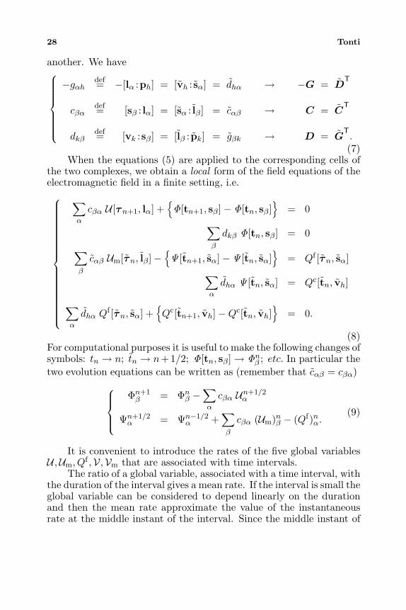
28 Tonti
another. We have
−gαhdef= −[lα :ph] = [vh : sα] = dhα → −G = D
T
cβαdef= [sβ : lα] = [sα : lβ] = cαβ → C = C
T
dkβdef= [vk :sβ] = [lβ : pk] = gβk → D = G
T.(7)
When the equations (5) are applied to the corresponding cells ofthe two complexes, we obtain a local form of the field equations of theelectromagnetic field in a finite setting, i.e.
∑α
cβα U [τn+1, lα] +Φ[tn+1, sβ]− Φ[tn, sβ]
= 0
∑β
dkβ Φ[tn, sβ] = 0
∑β
cαβ Um[τn, lβ]−Ψ [tn+1, sα]−Ψ [tn, sα]
= Qf [τn, sα]
∑α
dhα Ψ [tn, sα] = Qc[tn, vh]
∑α
dhα Qf [τn, sα] +Qc[tn+1, vh]−Qc[tn, vh]
= 0.
(8)For computational purposes it is useful to make the following changes ofsymbols: tn → n; tn → n+1/2; Φ[tn, sβ]→ Φn
β ; etc. In particular thetwo evolution equations can be written as (remember that cαβ = cβα)
Φn+1β = Φn
β −∑α
cβα Un+1/2α
Ψn+1/2α = Ψn−1/2
α +∑β
cβα (Um)nβ − (Qf)nα.(9)
It is convenient to introduce the rates of the five global variablesU ,Um, Qf ,V,Vm that are associated with time intervals.
The ratio of a global variable, associated with a time interval, withthe duration of the interval gives a mean rate. If the interval is small theglobal variable can be considered to depend linearly on the durationand then the mean rate approximate the value of the instantaneousrate at the middle instant of the interval. Since the middle instant of
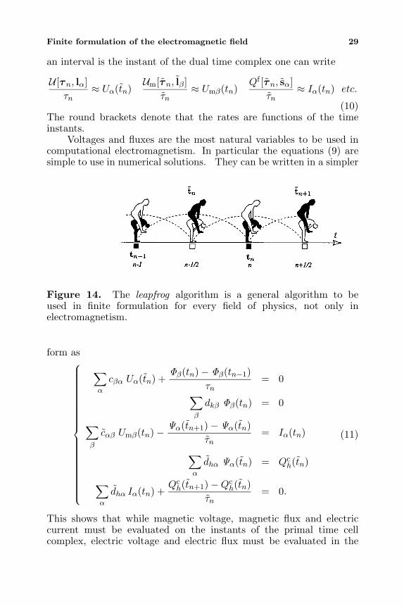
Finite formulation of the electromagnetic field 29
an interval is the instant of the dual time complex one can write
U [τn, lα]τn
≈ Uα(tn)Um[τn, lβ]
τn≈ Umβ(tn)
Qf [τn, sα]τn
≈ Iα(tn) etc.
(10)The round brackets denote that the rates are functions of the timeinstants.
Voltages and fluxes are the most natural variables to be used incomputational electromagnetism. In particular the equations (9) aresimple to use in numerical solutions. They can be written in a simpler
Figure 14. The leapfrog algorithm is a general algorithm to beused in finite formulation for every field of physics, not only inelectromagnetism.
form as
∑α
cβα Uα(tn) +Φβ(tn)− Φβ(tn−1)
τn= 0
∑β
dkβ Φβ(tn) = 0
∑β
cαβ Umβ(tn)−Ψα(tn+1)−Ψα(tn)
τn= Iα(tn)
∑α
dhα Ψα(tn) = Qch(tn)
∑α
dhα Iα(tn) +Qch(tn+1)−Qc
h(tn)τn
= 0.
(11)
This shows that while magnetic voltage, magnetic flux and electriccurrent must be evaluated on the instants of the primal time cellcomplex, electric voltage and electric flux must be evaluated in the
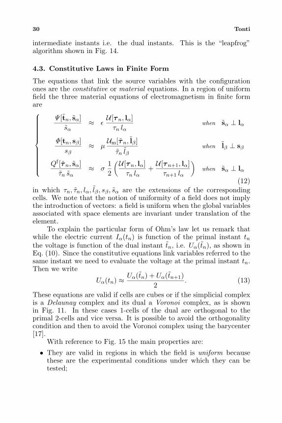
30 Tonti
intermediate instants i.e. the dual instants. This is the “leapfrog”algorithm shown in Fig. 14.
4.3. Constitutive Laws in Finite Form
The equations that link the source variables with the configurationones are the constitutive or material equations. In a region of uniformfield the three material equations of electromagnetism in finite formare
Ψ [tn, sα]sα
≈ εU [τn, lα]
τn lαwhen sα ⊥ lα
Φ[tn, sβ]sβ
≈ µUm[τn, lβ]
τn lβwhen lβ ⊥ sβ
Qf [τn, sα]τn sα
≈ σ12
(U [τn, lα]τn lα
+U [τn+1, lα]
τn+1 lα
)when sα ⊥ lα
(12)in which τn, τn, lα, lβ, sβ, sα are the extensions of the correspondingcells. We note that the notion of uniformity of a field does not implythe introduction of vectors: a field is uniform when the global variablesassociated with space elements are invariant under translation of theelement.
To explain the particular form of Ohm’s law let us remark thatwhile the electric current Iα(tn) is function of the primal instant tnthe voltage is function of the dual instant tn, i.e. Uα(tn), as shown inEq. (10). Since the constitutive equations link variables referred to thesame instant we need to evaluate the voltage at the primal instant tn.Then we write
Uα(tn) ≈Uα(tn) + Uα(tn+1)
2. (13)
These equations are valid if cells are cubes or if the simplicial complexis a Delaunay complex and its dual a Voronoi complex, as is shownin Fig. 11. In these cases 1-cells of the dual are orthogonal to theprimal 2-cells and vice versa. It is possible to avoid the orthogonalitycondition and then to avoid the Voronoi complex using the barycenter[17].
With reference to Fig. 15 the main properties are:
• They are valid in regions in which the field is uniform becausethese are the experimental conditions under which they can betested;
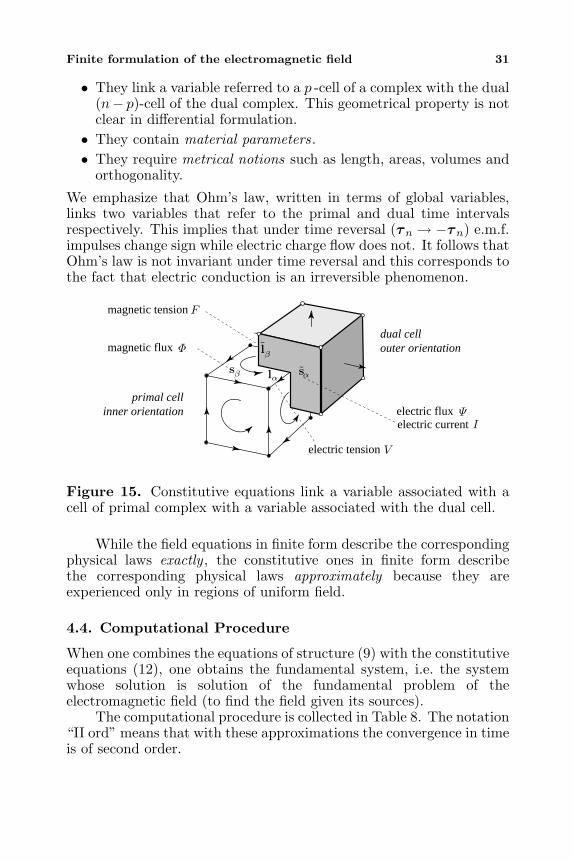
Finite formulation of the electromagnetic field 31
• They link a variable referred to a p -cell of a complex with the dual(n− p)-cell of the dual complex. This geometrical property is notclear in differential formulation.
• They contain material parameters.• They require metrical notions such as length, areas, volumes and
orthogonality.
We emphasize that Ohm’s law, written in terms of global variables,links two variables that refer to the primal and dual time intervalsrespectively. This implies that under time reversal (τn → −τn) e.m.f.impulses change sign while electric charge flow does not. It follows thatOhm’s law is not invariant under time reversal and this corresponds tothe fact that electric conduction is an irreversible phenomenon.
Velectric tension
Fmagnetic tension
magnetic flux Φ
electric flux Ψelectric current I
primal cellinner orientation
dual cellouter orientation
l
β
sα
l
αsβ
Figure 15. Constitutive equations link a variable associated with acell of primal complex with a variable associated with the dual cell.
While the field equations in finite form describe the correspondingphysical laws exactly , the constitutive ones in finite form describethe corresponding physical laws approximately because they areexperienced only in regions of uniform field.
4.4. Computational Procedure
When one combines the equations of structure (9) with the constitutiveequations (12), one obtains the fundamental system, i.e. the systemwhose solution is solution of the fundamental problem of theelectromagnetic field (to find the field given its sources).
The computational procedure is collected in Table 8. The notation“II ord” means that with these approximations the convergence in timeis of second order.
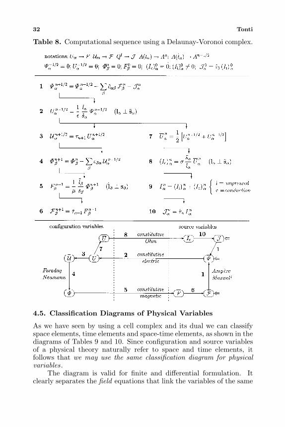
32 Tonti
Table 8. Computational sequence using a Delaunay-Voronoi complex.
4.5. Classification Diagrams of Physical Variables
As we have seen by using a cell complex and its dual we can classifyspace elements, time elements and space-time elements, as shown in thediagrams of Tables 9 and 10. Since configuration and source variablesof a physical theory naturally refer to space and time elements, itfollows that we may use the same classification diagram for physicalvariables.
The diagram is valid for finite and differential formulation. Itclearly separates the field equations that link the variables of the same
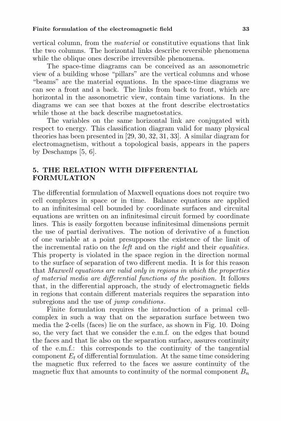
Finite formulation of the electromagnetic field 33
vertical column, from the material or constitutive equations that linkthe two columns. The horizontal links describe reversible phenomenawhile the oblique ones describe irreversible phenomena.
The space-time diagrams can be conceived as an assonometricview of a building whose “pillars” are the vertical columns and whose“beams” are the material equations. In the space-time diagrams wecan see a front and a back. The links from back to front, which arehorizontal in the assonometric view, contain time variations. In thediagrams we can see that boxes at the front describe electrostaticswhile those at the back describe magnetostatics.
The variables on the same horizontal link are conjugated withrespect to energy. This classification diagram valid for many physicaltheories has been presented in [29, 30, 32, 31, 33]. A similar diagram forelectromagnetism, without a topological basis, appears in the papersby Deschamps [5, 6].
5. THE RELATION WITH DIFFERENTIALFORMULATION
The differential formulation of Maxwell equations does not require twocell complexes in space or in time. Balance equations are appliedto an infinitesimal cell bounded by coordinate surfaces and circuitalequations are written on an infinitesimal circuit formed by coordinatelines. This is easily forgotten because infinitesimal dimensions permitthe use of partial derivatives. The notion of derivative of a functionof one variable at a point presupposes the existence of the limit ofthe incremental ratio on the left and on the right and their equalities.This property is violated in the space region in the direction normalto the surface of separation of two different media. It is for this reasonthat Maxwell equations are valid only in regions in which the propertiesof material media are differential functions of the position. It followsthat, in the differential approach, the study of electromagnetic fieldsin regions that contain different materials requires the separation intosubregions and the use of jump conditions.
Finite formulation requires the introduction of a primal cell-complex in such a way that on the separation surface between twomedia the 2-cells (faces) lie on the surface, as shown in Fig. 10. Doingso, the very fact that we consider the e.m.f. on the edges that boundthe faces and that lie also on the separation surface, assures continuityof the e.m.f.: this corresponds to the continuity of the tangentialcomponent Et of differential formulation. At the same time consideringthe magnetic flux referred to the faces we assure continuity of themagnetic flux that amounts to continuity of the normal component Bn
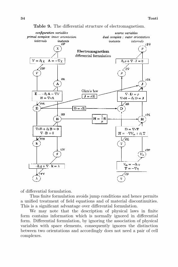
34 Tonti
Table 9. The differential structure of electromagnetism.
of differential formulation.Thus finite formulation avoids jump conditions and hence permits
a unified treatment of field equations and of material discontinuities.This is a significant advantage over differential formulation.
We may note that the description of physical laws in finiteform contains information which is normally ignored in differentialform. Differential formulation, by ignoring the association of physicalvariables with space elements, consequently ignores the distinctionbetween two orientations and accordingly does not need a pair of cellcomplexes.
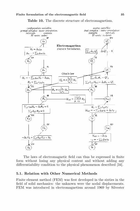
Finite formulation of the electromagnetic field 35
Table 10. The discrete structure of electromagnetism.
The laws of electromagnetic field can thus be expressed in finiteform without losing any physical content and without adding anydifferentiability condition to the physical phenomenon described [34].
5.1. Relation with Other Numerical Methods
Finite element method (FEM) was first developed in the sixties in thefield of solid mechanics: the unknown were the nodal displacements.FEM was introduced in electromagnetism around 1969 by Silvester
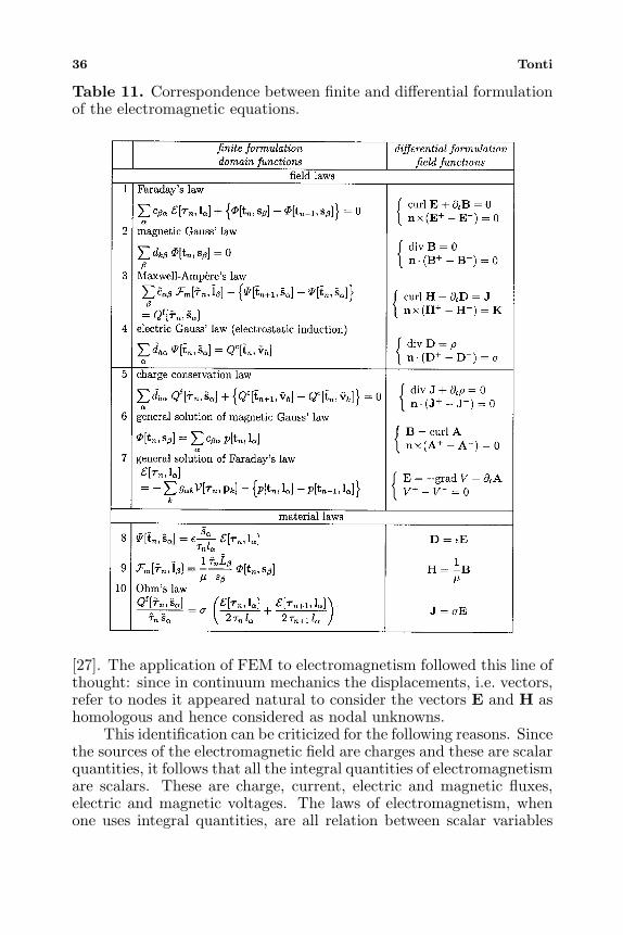
36 Tonti
Table 11. Correspondence between finite and differential formulationof the electromagnetic equations.
[27]. The application of FEM to electromagnetism followed this line ofthought: since in continuum mechanics the displacements, i.e. vectors,refer to nodes it appeared natural to consider the vectors E and H ashomologous and hence considered as nodal unknowns.
This identification can be criticized for the following reasons. Sincethe sources of the electromagnetic field are charges and these are scalarquantities, it follows that all the integral quantities of electromagnetismare scalars. These are charge, current, electric and magnetic fluxes,electric and magnetic voltages. The laws of electromagnetism, whenone uses integral quantities, are all relation between scalar variables
Finite formulation of the electromagnetic field 37
and then they are expressed by scalar equations. If this is so, why dowe commonly use vector quantities? The reason can be found in thefact that there are physical variables that refer to lines and surfaces:this is the case of electric and magnetic voltages, electric and magneticfluxes alongside with currents. Since for every space point there isan infinity of directions one is led to introduce at every space pointa vector to evaluate the integral variable referred to a line and to asurface by the scalar product of the field vector at the point and thevectors dL and dS that describe the geometrical elements, i.e,
U [L] =
∫LE · dL Φ[S] =
∫SB · dS
Um[L] =∫LH · dL Ψ [S] =
∫SD · dS I[S] =
∫SJ · dS.
(14)On the contrary in continuum mechanics the sources of the field
are forces, i.e. vectors. This implies that all global variables ofcontinuum mechanics are vectors. Such are displacements, velocities,relative displacements, relative velocities, surface and volume forces,momenta, etc. The relative displacements of two points depend on thevector connecting the points. The force across a surface depends onthe space orientation of the surface. This fact leads us to introducesecond rank tensors to express the dependence of such vector quantitieson the vectors that describe the lines and the surfaces: such arethe strain tensor, the strain-rate tensor and the stress tensor. Incontinuum mechanics, where finite elements were born, displacementsu and forces f are vectors associated with points (mesh nodes). Inelectromagnetism the vectors E and H, which are associated withlines are not homologous to the vectors of continuum mechanics. Thevectors in electromagnetism play the same role as tensors in continuummechanics. Stated in other words: the vectors of electromagnetism arenot the homologous of the vectors of continuous mechanics.
A numerical treatment of physical phenomena that does not takeinto account these differences is an “act of violence” on the physicsof the problem and gives rise to inconvenients. This was the case ofnumerical treatment of electromagnetism by the finite element method:the vectors E and H have been applied to nodes. This gives rise tospurious solutions in electromagnetic guide waves with two dielectricsas well as in three-dimensional electromagnetic problems [28, 11].Much time and ingenuity has been spent on finding the reason forsuch spurious solutions.
A further negative feature connected with field vectors isencountered in the solution of diffraction problems, where it is foundthat the electromagnetic field vectors may become infinite at sharp
38 Tonti
edges of a diffracting obstacle while electromagnetic energy in any finitedomain must be finite: this is the so called edge condition [19].
Faced with the appearance of spurious solutions, in 1982 Bossavitand Verite [1] suggested abandoning the nodal values of field vectorsE,H. Using tetrahedral meshes, they introduced, in electromagneticcomputations, electromotive and m.m.f. along the edges of thetetrahedra [4, p.XV]. This was the birth of the edge element method(EEM) introduced by Bossavit in 1988 [2]. This method is an extensionof FEM and it uses a single mesh. The same authors realized that theuse of such global variables is in harmony with the use of the exteriordifferential forms. Taking the latter as a starting point, the finite formwas achieved via special differential forms, the so called Whitney formsfollowing a suggestion of Kotiuga [13].
A completely different method to give a finite formulation toMaxwell equations was introduced in 1966 by Yee [43]. He startedconsidering a Cartesian mesh and associating the three componentsEx, Ey, Ez located in the middle of the edges and the three componentsHx, Hy, Hz located in the center of the faces. Doing so he introduced apair of dual grids, G and G, later called the electric and magnetic grids.He considered the two differential equations containing curlE andcurlH and discretized them using finite differences. Yee’s method wascalled Finite Differences in Time Domain (FDTD). It is a refinementof FDM based on a pair of dual Cartesian meshes and on an ad hocassociation of physical variables to the two meshes.
The FDTD method of Yee has been developed by Weiland since1977 [39]. The author, in a paper of 1984 [40], [41] initiated the useof Maxwell equations in integral form. The method has been namedFinite Integration Theory (FIT) and is the method used in the programMAxwell Finite Integration Algoritm (MAFIA). The integral form wasapproximated considering the tangential component Et in the middleof the edges of G and the normal component Bn in the middle of thefaces of G. The dual mesh G, called the magnetic grid , appeared as anatural completion of the mesh G, called the electric grid to make thenormal component Bn, which is normal to the faces of G, tangentialto the edges of G [40, p.250]. In the FIT method spurious solutions donot appear [41, p.229].
In 1996 Weiland [42] takes an important step forward whenhe introduces integrated field as state variables rather than directlyfield components. In other words the unknowns are now vectorslike (e1, e2, ...en) where ek are voltages along the edges. Doing sohe obtained an exact implementation of Maxwell’s equations. Inthe words of Weiland “The outstanding features of Maxwell’s GridEquations (MGE) when compared with other numerical methods for
Finite formulation of the electromagnetic field 39
solving field problems is that this set of matrix equations is a consistentfinite representation of the original field equations in that sense thatbasic properties of analytical fields are maintained when moving fromIR3 to G, G.” Weiland went on in 1996 to consider electric andmagnetic voltages using a pair of dual meshes while Bossavit [1] didthe same in 1982 but on a single mesh. We can see that, starting fromdifferent points of departure, computational electromagnetism evolvedtowards the use of a pair of dual meshes and the use of global variables.
Outside electromagnetism, in fluid dynamics, the Finite VolumeMethod (FVM) evolved in the same direction. Here one use a pair ofdual meshes and make use of global variables. We remark that FDM,FDTD, FIT and FVM use mainly cartesian meshes while EEM usessimplicial complexes.
The finite formulation of electromagnetism we have presented inthis paper, starting from an analysis of global physical variables, joinsthe methods inaugurated by Yee and Bossavit.
5.2. The Cell Method
The main feature of finite formulation we have presented is the use ofglobal variables that are domain functions instead of local variables,i.e. field functions. This implies that we do not use differentialequations or differential forms. The solutions to field problems can beachieved considering a simplicial complex K of Delaunay type and itsorthogonal dual K of Voronoi. This presupposes a Delaunay-Voronoimesh generator in two or in three dimensions. This choice permitsa simple implementation of material equations, at least for isotropicmedia, because they link a physical variable associated with a p -cellwith another variable associated with the dual (n − p)-cell when thecells are orthogonal.
Variables. The variables used are: magnetic flux Φ; electric flux Ψ ;electric voltage impulse U and magnetic voltage impulse Um.
Field equations. Field equations are implemented as follows:
• the Maxwell-Ampere’s and Gauss’ magnetic laws on dual cells;• the Faraday’s law and Gauss’ electric laws on primal cells.
Field equations have an exact implementation because we use globalvariables in space and time.
Constitutive equations. The field inside every simplex issupposed to be uniform and the material homogeneous so that the
40 Tonti
material equations are exact in every simplex: the only approximationwe carry out is to assume uniformity of the field inside simplexes.
Material discontinuities. The working region can be filledwith different materials. It is always possible to construct a simplicialcomplex whose simplexes do not cross the separation surfaces but havea face that laying on them, as shown in Fig. 10. This automaticallyassures that jump conditions will be satisfied because voltages andfluxes on the edges and faces respectively are the same for two adjacentcells.
A numerical method based on these rules will be called the cellmethod.
6. CONCLUSION
We have shown that it is possible to build a finite formulation tothe electromagnetic equations directly based on experimental laws,i.e. without passing from the differential formulation. This put intoevidence some features that are not commonly considered in thedifferential formulation. First of all we use global variables instead of(local) field variables. The global variables are associated with spaceand time elements endowed with inner and outer orientation. Thesetwo kind of orientations are not explicit in the differential formulation.As a consequence of this association, global variables are domainfunctions while field functions are point functions. Coordinate systems,that are a natural framework for field functions, are substituted bycell-complexes. The role of orthogonal coordinate systems is playedby a pair of Delaunay-Voronoi complexes for which the p -cells of onecomplex are orthogonal to the (n−p)-cells of the other.
The fact that some global variables are referred to space and timeelements endowed with inner orientation and other to outer orientationimplies that some global variables are naturally referred to the elementsof the primal complex and other to the elements of the dual one. Thisgives a fundamental role to a pair of cell complexes, a notion that islacking in the differential formulation.
The analysis we have done permits to clearly separate topologicalequations from phenomenological equations.
The topological equations link physical variables referred to thesame cell complex, primal or dual, and are expressed by the operatorsgradient, curl and divergence in the differential setting. Topologicalequations are independent of metrical notions: a fact that is notusually stressed in the differential formulation. In fact the notionof gradient, curl and divergence are usually presented in a metricalcontext. This metric-independence, on the contrary, it stressed using
Finite formulation of the electromagnetic field 41
exterior differential forms.The phenomenological equations, i.e. the so called material or
constitutive equations, link a variable associated with a p -dimensionalcell with another variable associated with the dual (n−p)-dimensionalcell. Contrary to the topological equations they depend on metricalnotions. This is another feature hidden by differential formulation.
In the theory of differential forms the topological equations onthe primal complex (inner orientation) are expressed by exteriordifferential forms while those on the dual complex (outer orientation)are expressed by twisted or odd or impair exterior differential forms.
The natural role of two cell complexes is of primary importancein computational electromagnetism and gives a justification to the useof staggered meshes as done in FDTD.
ACKNOWLEGMENT
The author is grateful to Prof. A. Nicolet, L. Mania and to the engineerM. Marrone for their useful advices. The author is also particularlygrateful to the colleagues F. Bellina and F. Trevisan and M. Guarnierifor their careful review of the final draft of the manuscript and for theirhelpful suggestions.
REFERENCES
1. Bossavit, A. and J. C. Verite, “A mixed FEM-BIEM methodto solve eddy-currents problems,” IEEE Trans. on Magnetics,Vol. 18, 431–435, 1982.
2. Bossavit, A., “A rationale for ‘edge-elements’ in 3-D fieldscomputations,” IEEE Trans. on Magnetics, Vol. 24, No. 1, 74–79, 1988.
3. Bossavit, A., C. Emson, and I. D. Mayergoyz, MethodesNumeriques en Electromagnetisme, Eyrolles, 1991.
4. Bossavit, A. and C. Emson, Computational Electromagnetism,Academic Press, 1998.
5. Deschamps, G. A., “Electromagnetics and differential forms,”Proceedings of the IEEE, Vol. 69, No. 6, 676–696, 1981.
6. Deschamps, G. A. and R. W. Ziolkowski, “Comparison of Cliffordand Grassmann algebras in applications to electromagnetism,”Clifford algebras and their Applications in Mathematical Physics,J. S. R. Chisholm and A. K. Common (eds.), 501–515, Reidel PublComp., 1986.
42 Tonti
7. Fleury, P. and J. P. Mathieu, Elettrostatica, Corrente Continua,Magnetismo, Zanichelli, Vol. 6, 1970.
8. Fouille, A., Electrotecnique a L’usage des Ingenieurs, Dunod,1961.
9. Hallen, E., Electromagnetic Theory, Chapman & Hall, 1962.10. Ingarden, R. S. and A. Jamiolkowsky, Classical Electrodynamics,
Elsevier, 1985.11. Jiang, B., J. Wu, and L. A. Povinelli, “The origin of
spurious solutions in computational electromagnetics,” Journal ofComputational Physics, Vol. 125, 104–123, 1996.
12. Jefimenko, O. D., Electricity and Magnetism, Appleton-Century-Crofts, 1966.
13. Kotiuga, P. R., “Hodge decomposition and computationalelectromagnetics,” Thesis, Department of Electrical Engineering,McGill University, Montreal, 1984.
14. Kron, G., “Equivalent circuits of the field equations of Maxwell,”Proc. IRE, Vol. 32, 289–299, 1944.
15. Kron, G., “The frustrating search for a geometrical model ofelectrodynamic networks,” Tensor, Vol. 13, 111–128, 1963.
16. Langevin, P., “Sur la nature des grandeurs et les choix d’unsysteme d’unites electriques,” Bull. Soc. Francaise de Physique,Vol. 164, 9, 1922. Reprinted in Oeuvres Scientifiques de PaulLangevin, 493–505, Centre Nationale de la Recerque Scientifique,1950.
17. Marrone, M., “Computational aspects of cell method inelectrodynamics,” this volume.
18. Maxwell, J. C., Traite Elementaire d’electricite, Gauthier Villars,1884.
19. Meixner, J., “The behaviour of electromagnetic fields at edges,”IEEE Trans. Antennas Propag., Vol. 20, No. 4, 442–446, 1972.
20. Pauli, W., Elettrodinamica, translation of Vorlesung Elektrody-namik, Boringhieri, 1964.
21. Penfield, P. and H. Haus, Electrodynamics of Moving Media,M.I.T. Press, 1967.
22. Perucca, E., Fisica Generale e Sperimentale, IV edizione, Vol. 2,Unione Tipografica Editrice Torinese, 1945.
23. Pohl, R. W., Physical Principles of Electricity and Magnetism,Blackie and Son, 1930.
24. Post, E. J., Geometry and Physics: A Global Approach, Burge,(ed.), Problems in the Foundation of Physics, Vol. 4, Springer-

Finite formulation of the electromagnetic field 43
Verlag, 1971.25. Rojansky, V., Electromagnetic Fields and Waves, Dover, 1979.26. Schelkunoff, S. A., Electromagnetic Fields, Blaisdell, 1963.27. Silvester, P., “Finite element solution of homogeneous waveguides
problems,” Alta Frequenza, Vol. 38, 313–317, 1969.28. Sun, D. K., J. Manges, X Yuan, and Z. Cendes, “Spurious modes
in finite-elements methods,” IEEE Trans. Ant. Propag., Vol. 37,No. 5, 12–24, 1995.
29. Tonti, E., “On the mathematical structure of a large class ofphysical theories,” Rend. Acc. Lincei, Vol. LII, 48–56, 1972.
30. Tonti, E., “A mathematical model for physical theories,” Rend.Acc. Lincei, Vol. LII, Part I, 175–181, Part II, 350–356, 1972.
31. Tonti, E., “On the formal structure of physical theories,” Preprintof the Italian National Research Council, 1975 (unpublished).
32. Tonti, E., “The algebraic-topological structure of physicaltheories,” Conference on Symmetry, Similarity and GroupTheoretic Methods in Mechanics, 441–467, Calgary, Canada, 1974.
33. Tonti, E., “The reasons for analogies between physical theories,”Appl. Mat. Modelling, Vol. I, 37–50, 1976.
34. Tonti, E., “On the geometrical structure of electromagnetism,”Gravitation, Electromagnetism and Geometrical Structures, forthe 80th Birthday of A. Lichnerowicz, Edited by G. Ferrarese.Pitagora Editrice Bologna, 281–308, 1995.
35. Tonti, E., “Algebraic topology and computational electromag-netism,” Fourth International Workshop on the Electric and Mag-netic Fields: from Numerical Models to Industrial Applications,284–294, Marseille, 1998.
36. Truesdell, C. and R. Toupin, The Classical Field TheoriesHandbuck der Physik, Band III/1, Springer, 1960.
37. Van Dantzig, D., “Electromagnetism, independent of metricalgeometry,” Proc. Amsterdam Acad., Vol. 37, 521–525, 526–531,643–652, 825–836, 1934.
38. Veblen, O. and J. H. C. Whitehead, The Foundations ofDifferential Geometry, No. 29, 55–56, Cambr. Tracts, 1932.
39. Weiland, T., “Eine methode zur Losung der MaxwellschenGleichungen fur sechskomponentige felder auf diskreter basis,”AEU, Band 31, Heft 3, 1977.
40. Weiland, T., “On the numerical solution of Maxwell’s equationsand applications in the field of accelerator physics,” ParticleAccelerators, 245–292, 1984.

44 Tonti
41. Weiland, T., “On the unique numerical solution of maxwellianeigenvalue problems in three dimensions,” Particle Accelerators,227–242, 1985.
42. Weiland, T., “Time domain electromagnetic field computationwith finite difference methods,” Int. J. of Num. Modelling, Vol. 9,295–319, 1996.
43. Yee, K. S., “Numerical solution of initial boundary value problemsinvolving Maxwell’s equations in isotropic media,” IEEE Trans.Antennas Propag., Vol. 14, 302–307, 1966.
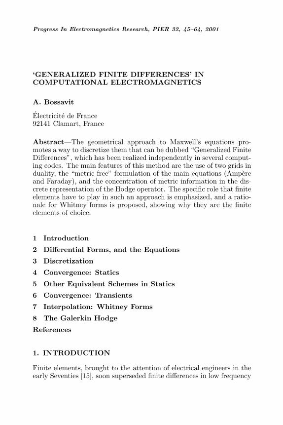
Progress In Electromagnetics Research, PIER 32, 45–64, 2001
‘GENERALIZED FINITE DIFFERENCES’ INCOMPUTATIONAL ELECTROMAGNETICS
A. Bossavit
Electricite de France92141 Clamart, France
Abstract—The geometrical approach to Maxwell’s equations pro-motes a way to discretize them that can be dubbed “Generalized FiniteDifferences”, which has been realized independently in several comput-ing codes. The main features of this method are the use of two grids induality, the “metric-free” formulation of the main equations (Ampereand Faraday), and the concentration of metric information in the dis-crete representation of the Hodge operator. The specific role that finiteelements have to play in such an approach is emphasized, and a ratio-nale for Whitney forms is proposed, showing why they are the finiteelements of choice.
1 Introduction
2 Differential Forms, and the Equations
3 Discretization
4 Convergence: Statics
5 Other Equivalent Schemes in Statics
6 Convergence: Transients
7 Interpolation: Whitney Forms
8 The Galerkin Hodge
References
1. INTRODUCTION
Finite elements, brought to the attention of electrical engineers in theearly Seventies [15], soon superseded finite differences in low frequency
46 Bossavit
applications, thanks to their ability to model complex shapes. Still,in wave propagation problems, Yee’s classical FDTD method [22,16] continues to reign. This and other facts like the efficiency ofthe MAFIA group of codes [19], Tonti’s “elementless” demonstrationsoftware [18], the interest for “lattice oriented” methods [17], seem tosuggest that finite elements, and the variational method, may not bethat dominant a paradigm after all. Are finite differences back?
We purport to show that, when seeing things from a geometricalpoint of view, there is no such sharp contrast. Finite elements don’thold the foreground, but they are nonetheless essential.
The geometrical approach to computational electromagnetismcan be traced back to Kottler, Cartan, and van Dantzig [6], whoindependently pointed out, Post [14] tells us, the metric-free characterof the two main Maxwell equations, ∂tB + rotE = 0 (Faraday’s law)and −∂tD+rotH = J (Ampere’s theorem). These make sense withoutany metric structure in 3D space, whereas metric is needed to accountfor constitutive laws such as B = µH and D = εE. (This is just astrue of Ohm’s law J = σE, but we shall ignore it for simplicity, andassume all currents given.) The Hodge operator, by which they canbe expressed, depends on the metric structure. More, it brings in, onemay argue [5, 4], the metric structure.
This fact explains the close similarity of independently proposedschemes (see e.g., [9, 18, 19]) as regards the discretization of Faradayand Ampere: These “grid equations”, to use Weiland’s expression [20],are forced on us, so to speak, as soon as a discretization mesh isthere. What makes the variety of methods and distinguishes numericalschemes is, mainly, their treatment of the Hodge operator. Each ofthem is characterized by a specific “discrete Hodge”. Finding underwhich conditions the latter will produce a stable and convergent schemeappears, therefore, as the central problem of the theory, the one onwhich error analysis should focus.
Which is where finite elements enter the stage: not as aprerequisite, as in the Galerkin approach, but as a theoretical tool forwhat is, in this perspective, a task for professionals—error analysis.The whole approach takes on a different flavor, which “generalizedfinite differences” (GFD) seems to describe well. Moreover, fromthis vantage point, the Galerkin approach, as well as finite volumemethods, do not appear so different from the Darmstadt school’s FiniteIntegration Technique: the Galerkin method, as realized by WETD [10]in wave problems, is a case of GFD, with a particular dual mesh (the“barycentric” one) and a particular discrete Hodge.
I’d wish to show that, even at this late stage, geometry illuminatesthe way. Appropriate finite elements for differential forms (the
GFD in computational electromagnetics 47
Whitney complex) can be derived, by geometric reasoning. Theyanswer requirements about interpolation that almost dictate theirspecific form. I will point in particular to a unifying property ofWhitney forms, that they constitute, in a precise sense, a partitionof unity.
This makes Section 8 of the present paper. Before that, one recallsthe differential-geometric way to state Maxwell’s equations (Section 2)and to discretize them (Section 3), and convergence is examined instatics (Section 4) and transients (Section 6), within a formalism thatcan accommodate different discrete Hodge operators. A digression(Section 5) shows how so-called “mixed” methods fit in this picture.Section 7 introduces Whitney forms, with a new twist: they comein answer to the natural question “how to associate a p-chain with ap-manifold”.
2. DIFFERENTIAL FORMS, AND THE EQUATIONS
Let’s briefly recall why differential forms, not vector fields, are theright geometrical objects in electromagnetic theory. The main idea isthat a physical entity, as identified via empirical phenomena, should berepresented by the simplest possible mathematical entity. When theelectric field, say, is represented by a vector field E, the electromotiveforce (emf, expressed in volts) along an oriented curve c is
∫c τ · E,
where τ denotes the unit tangent vector. (Orienting c, here done byhaving chosen one of the two possible τs, is essential.) The physicalfield is entirely characterized (from the point of view of what can beknown about it, what can be measured) by its emf’s, which we denoteby
∫c e, for all c’s. In the equality
∫c e =
∫c τ · E, E must change if
the dot product changes, in order to preserve the emf at the left-handside. Therefore what is mathematically cogent is not E (called herea “proxy” field for this reason), but the map from curves to emf’s,c →
∫c e ≡
∫c τ · E. Such a map (additive with respect to c and
continuous with respect to deformations of c) is called a differentialform of degree 1, or 1-form, and we reserve the notation e for it. One-forms add, e + e′ being the map c →
∫c e +
∫c e′, and have scalar
multiples, λe being c→ λ∫c e.
There are p-forms for all values of p from 0 to 3. In particular,a mapping from oriented surfaces to real numbers, with similarproperties as above, is a 2-form. The magnetic flux b is one, whichassigns to an oriented surface S the flux
∫S b. Three-forms map oriented
volumes to real numbers, and 0-forms map points to numbers.Orientation, in each of these cases, is an attribute of the manifold
on which integration is performed, not of ambient 3D space. We say
48 Bossavit
the manifold has inner orientation to stress that. (The orientation of apoint is just a sign, + or −.) To each p-manifold its own orientation. Inthe case of a manifold and its boundary, however, orienting one of themcanonically orients the other one, because “from inside to outside”,relative to the manifold, is an intrinsic notion. For instance, innerorientation of the rim ∂S of a surface S derives from an orientation ofthe latter. We say that independently assigned orientations “match”when they conform to this canonical choice.
Faraday’s experiment can at this stage be accounted for by
∂t
∫Sb+
∫∂Se = 0 (1)
for all inner-oriented surfaces S, provided the orientation of (each pieceof) ∂S matches that of S.
Note that we refrained to confuse inner orientation of S with a“crossing direction” through S: the two notions can indeed be linked,via orientation of ambient space, but the latter is physically irrelevant.Giving a crossing direction, however, is right if the concept one wantsto capture is that of flow of something, electric charge for instance,through the surface. A surface Σ thus equipped is said to be outeroriented. Additive continuous maps from outer-oriented surfaces toreals are called twisted 2-forms. Current-density j is such a map, andthe number
∫Σ j it assigns to Σ is the intensity through Σ (expressed
in amperes).To properly define this kind of orientation, one begins with
vector subspaces: Outer orientation of one is, by definition, innerorientation of any of its complements. The notion immediately extendsto manifolds. In particular, an outer oriented line γ is one equippedwith a sense of “which way to turn around it”, i.e., an inner orientationof its transverse planes. Additive continuous maps from such lines toreals are called twisted 1-forms. They are the right objects to representthe magnetic field strength, here denoted h. The number
∫γ h is called
“the magnetomotive force (mmf) over γ”, expressed in amperes. As forthe displacement current d, it’s a twisted 2-form like j, and Ampere’stheorem is the statement
−∂t∫Σd+
∫∂Σh =
∫Σj, (2)
for all outer-oriented surfaces Σ, provided the outer orientation of (eachpiece of) ∂Σ matches that of Σ.
Our discretization strategy will consist in enforcing (1) and (2),which in theory must hold for all surfaces, inner- or outer-oriented asthe case may be, for a selected family of such surfaces, those generated
GFD in computational electromagnetics 49
by the faces of two interlocked meshes. But first, we need to deal withconstitutive laws. It’s now (but only now) that a metric is necessary.
Consider a small plane patch S and a small straight segment γ,at right angle at their intersection x. Assume an inner orientation ofS (any of the two possible ones) and take it as outer orientation of γ.Now let a twisted 1-form h be given. Thus knowing the value of
∫γ h,
we set ∫Sb = µx
area(S)length(γ)
∫γh, (3)
where µx is the permeability at point x, if well-defined there.(Discontinuities of µ are a minor difficulty, to be resolved later, cf. (10)below.) This extends to any surface S (chop it into small patches, formRiemann sums, and go to the limit) and thus defines a straight 2-formb. Hence a (linear) map from twisted 1-forms to straight 2-forms, whichwe call the µ-related Hodge operator, and shall simply denote by µ,since there is no ambiguity about the status of µ as an operator, not ascalar, in such an expression as b = µh. (We’ll use ν for the inverse ofµ, such that h = νb.) There is also an ε-related Hodge operator, withsimilar definition.
Let’s emphasize the importance of metric elements in (3), length,area, and especially, orthogonality: In terms of the vector proxies Band H, (3) would translate as n · B = µ τ · H, where n and τ area normal and a tangent unit vector respectively, i.e., n · H = τ · Hwhatever H, i.e., n = τ , which does require orthogonality between γand S.
3. DISCRETIZATION
Now let’s address the problem of waves emitted from an antenna andreflecting off the perfectly conductive walls of a bounded cavity D.This means solving (1) and (2), together with the constitutive laws
d = ε e, h = νb, (4)
for a given current density j inside D, null up to t = 0, plus∫ce = 0 for all curves c lying in ∂D, (5)
which expresses the boundary condition. Let’s show how the foregoingconsiderations lead towards a natural extension of Yee’s scheme.
Suppose a pair of meshes, both made of adjacent cells, withsmooth, but not necessarily plane, common faces. (We’ll say “p-cells”,with p = 0 to 3, and refer to them as nodes, edges, faces, and volumes.
50 Bossavit
Note that edges can be curved, or crooked, and that 2-cells are notnecessarily triangles or squares.) Arrange them so that p-cells of one(the “primal” mesh) are in 1–1 correspondence with (n−p)-cells of theother (called the “dual” mesh). As a rule, this is done by having edgesof one traverse faces of the other. Provide each primal p-cell with itsown (arbitrary) inner orientation, which automatically outer-orientsthe corresponding dual (n−p)-cell. (The 2-cell dual to e is e, the 1-celldual to f is f .) Call Re
f the incidence number of primal edge e to facef , defined as 0 if the boundary ∂f does not contain e, and ±1 if itdoes, the sign depending on whether orientations match or not. Hencea rectangular incidence matrix R, entries of which are ±1 or 0.
Next, assign real time-dependent degrees of freedom (DoF) toedges and faces: bf and ee are meant to approximate the magneticflux
∫f b and the emf
∫e e, while hf and de, on the dual side, stand for
dual-edge mmf’s and dual-face electric fluxes (approximations of∫f h
and∫e d). Call e, b, h, d, as above, the arrays of such DoF’s, indexed
over sets of cells of the same kind. Similarly, j gathers the intensities jethrough dual faces e (which are not unknown, but data, in the presentrestricted context).
Now let’s apply the previously announced strategy: enforce (1) forall surfaces S made of an assembly of primal faces, which by additivityof the integrals means
∂t
∫fb+
∫∂fe = 0 for each primal face f.
By the very definition of R, this results in ∂tbf +∑eR
efee = 0 for each
f . Hence, putting that in matrix form, and by similar considerationsapplied to surfaces Σ made of dual faces,
∂tb + Re = 0, −∂td + Rth = j, (6)
where Rt is the transpose of R.These “network equations” reflect the topology of the interlocking
networks, but they don’t use any metric information. Neither do theyrequire any notion of finite element.
By duality, components of b and h, or d and e, sit at the sameplace. Therefore, a natural way to discretize the constitutive laws isto set up square symmetric matrices εε and νν (boldface) and to enforce
d = εε e, h = ννb. (7)
Then the “leapfrog scheme”
−εε (ek+1/2 − ek−1/2)/δt+ Rtννbk = jk, (bk+1− bk)/δt+ Rek+
1/2 = 0(8)
GFD in computational electromagnetics 51
(with b0 = 0 and e−1/2 = 0 at the beginning) solves the approximationproblem. How should εε and νν be constructed? Sparsity, which refletsthe local character of laws (4), is an obvious requirement, but beyondthis, diagonality of εε is desirable, because it makes the scheme explicit.Positive-definiteness of εε and νν is required for stability. With all that,convergence of (7), (8) towards (6), (7) when the time-step δt tends to0 is an easy matter. (The hard part is, of course, convergence of (6),(7) to (1), (2), (4). We shall face this task in Sections 4 and 6.)
There are essentially two ways1 to construct these matrices. Awell-known one is the Galerkin method, that we shall revisit below(Section 8), which takes for εε and νν the so-called “mass matrices” offinite element theory. With this choice, (7) and (8) are the “WETD”scheme [10]. But since εε here, though relatively sparse, is not diagonal,the explicit character of Yee’s method is lost.
Hence the interest for the second way [19, 18], in which one designsthe meshes to be mutually orthogonal, a concept2 which goes back toMaxwell [11], meaning that all cells are straight and that a primal celland its dual mate intersect at right angle. Then, in the case when εand µ are uniform, one sets εεee
′= 0 if e = e′, µµff
′= 0 if f = f ′, and
(cf. (3))
εεee = εarea(e)
length(e), µµff = µ
area(f)length(f)
, (9)
which does provide diagonal matrices εε and µµ. In the case of non-uniform coefficients, formulas such as
µµff =µ1µ2 area(f)
µ1length(f1) + µ2length(f2), (10)
where f1 and f2 are the parts of f belonging to the two volumesadjacent to f , apply instead. Of course, νν is the inverse of µµ.
We note that metric is needed in both procedures, and henceappears in the “network constitutive laws” (7).
Such rules as (9) or (10), which closely mimic the very definitionof the Hodge operator, are so natural that one might feel like claimingdiscretization without shape functions! Indeed, (7), (8) with (9) or(10) is the closest thing to the Yee scheme for staggered cellular grids,and we just derived it without using any shape function.
Yet, finite elements are needed. As we just saw, the constructionof the “discrete Hodge operators” εε and νν is not forced on us, theway (6) were. So if a rule for setting up εε and νν is proposed, by which1 See [8] for an attempt to go beyond this crude dichotomy.2 Not to be confused with that of an orthogonal grid a la Yee, with all edges parallel toone of the Cartesian axes.
52 Bossavit
one obtains square symmetric positive-definite—though not necessarilydiagonal—matrices, how do we assess the value of such a proposal?By proving the convergence of the scheme when both meshes areindefinitely refined, and this requires finite elements, as an analysisof the proof will show.
4. CONVERGENCE: STATICS
Let’s first deal with magnetostatics, which consists in finding a pairb, h such that
∫Sb = 0, b = µh,
∫∂Σh =
∫Σj, (11)
for all closed inner-oriented surfaces S and all outer-oriented surfacesΣ inside D. Since ∂Σ reduces to 0 for closed such surfaces, the givenj must satisfy
∫Σ j = 0 for all closed Σ. By the same discretization
strategy as above, this becomes
Db = 0, b = µµh, Rth = j, (12)
where D is the face-to-volumes incidence matrix, defined the same wayR was. (Since DR = 0, a fact with straightforward proof, (12) stemsfrom (6) in static situations.) Problem (12) has a unique solutionb,h, provided Gtj = 0, where G is the nodes-to-edges incidencematrix. (Again, RG = 0, therefore GtRt = 0, and hence the necessarycondition about j.)
We’ll need some notation: F is the set of “active” primal faces(excluding those of the boundary, on which bf = 0) and an expressionsuch as (b,h), with boldface parentheses, denotes the sum
∑f∈F bfhf .
An expression such as (b, h) refers to what would be, in terms of vectorproxies,
∫D B · H, a quantity which actually does not depend on the
metric (it’s∫D b ∧ h in differential geometric language). We’ll assume
simple topology of D, in which case not only RG = 0 and DR = 0,but ker(R) and ker(D) coincide with the ranges of G and R (proofsof these well-known properties can be found in [1], Chap. 5). As aconsequence, the orthogonality relation
Du = 0 and Rtv = 0⇒ (u,v) = 0 (13)
holds. Last, we denote by |||u|||ν and |||v|||µ the square roots of the quantities(ννu,u) and (µµv,v).
Let us denote by m the pair of interlocked meshes, and call“grain”, γm, the maximum diameter of all cells. Our purpose is tostudy bm, hm when γm tends to 0, while respecting the uniformity
GFD in computational electromagnetics 53
condition that there be a finite number of element shapes in the wholefamily of refinements of the initial coarse mesh. We adopt “m → 0”as a shorthand for that. We shall compare the computed DoF arrays,b and h, with arrays of the same kind, rmb =
∫f b : f ∈ F and
rmh = ∫f h : f ∈ F, composed of the fluxes and mmf’s of the
(unknown) solution of (11).Since
∫S b = 0 for all closed surfaces S, this applies to the boundary
of any primal 3-cell v (v for volume), hence the sum of face fluxes∑f Df
v
∫f b must vanish for all v. Similarly,
∫∂Σ h =
∫Σ j applies when
Σ is a dual 2-cell, which yields the relation∑f Re
f
∫f h =
∫e j. In matrix
form, all this results in Drmb = 0, Rtrmh = rmj ≡ j. Comparing with(12), we obtain
D(b− rmb) = 0, Rt(h− rmh) = 0, (14)
and
(b− rmb)− µµ(h− rmh) = (µµrm − rmµ)h ≡ µµ(rmν − ννrm)b. (15)
Now, let’s premultiply (15) by νν and take the ()-scalar product ofthis with (15) itself, side by side. Some algebra, using the orthogonality(13) that (14) implies, leads to
(νν(b−rmb),b−rmb)+(µµ(h−rmh),h−rmh)=((µµrm−rmµ)h, (rmν−ννrm)b),(16)
the cornerstone of the convergence proof, which we recast as
|||b− rmb|||2ν + |||h− rmh|||2µ = |||(ννrm− rmν)b|||2µ ≡ |||(µµrm − rmµ)h|||2ν (17)
to better suggest the geometric interpretation of this equality, and alsoits physical meaning: If we call “discrete energy” of b [resp. “discretecoenergy” of h] the quantity 1/2|||b|||2ν [resp. 1/2|||h|||2µ], we see thatthe “distance in energy” between the computed array of fluxes[resp. mmf’s] and the actual one tends to zero, provided the so-calledinconsistency error at the right-hand side of (17) tends to 0 with m.We rewrite the latter requirement, in less formal but more suggestivefashion, as
(ννrm−rmν)b→ 0 when m→ 0, (µµrm−rmµ)h→ 0 when m→ 0, (18)
for any 2-form b or twisted 1-form h, two equivalent properties whichexpress the consistency of the approximation scheme.
This is the core of the matter: a good discrete Hodge operatormust satisfy (18). Do the ones in (9) comply?
54 Bossavit
Yes, as easily verified thanks to a local computation, for which werevert again to vector proxies. First suppose that H is uniform in thevicinity of face f . The flux [(µµrm − rmµ)h]f then vanishes, because sowas the rationale behind the definition of µµ, back in (9). For a non-uniform H, now, a Taylor expansion about the point f ∩ f allows us tobound this quantity by Cγm area(f), where C depends on H but noton m, hence (same symbol C for all constants, with possibly differentvalues)
|||(µµrm − rmµ)h|||2ν ≤ C∑f
length(f)area(f)
γ2marea(f)2 ≤ Cγ2
mvolume(D).
This very rough estimate could be improved upon, by more finelytaking into account the local geometry, and by exploiting theuniformity of the mesh sequence, but it suffices to show that, indeed,(18) holds.
The same argument works for all reasonable ways to defineµµ, including the Galerkin method, to which we shall return, and“finite volume” approaches [13]. The important thing is to have theinconsistency (µµrm − rmµ)h vanish for locally uniform fields3.
Going back to (17), we see that |||b − rmb|||2ν behaves like γ2m when
m is refined. But this is hardly enough to prove convergence in anydefinite way. For this, one should build from the DoF arrays b and han approximation bm, hm of the field, and prove that both bm − band hm − h tend to 0 with m, in an appropriate sense. Settingbm = pmb and hm = pmh, where each pm is a linear map, not yetspecified, we may for instance require that both (ν(b− pmb), b− pmb)and (µ(h−pmh), h−pmh) tend to 0 with m (convergence “in energy”).Sufficient conditions on pm to this effect are the consistency condition:
pmrmb→ b, pmrmh→ h, in energy, when m→ 0, (19)
and the following inequalities:
α(νpmb, pmb) ≤ (ννb,b), α(µpmh, pmh) ≤ (µµh,h), (20)
for all b and h, where the constant α > 0 does not depend on m. Thisexpresses the stability of the approximation scheme. Convergence,now, is straightforward (Lax’s theorem): First, pm(b − rmb) → 0, by(20), then pmb → b, thanks to (19). Same argument about h. Notethat only L2 estimates came into play.
So what about the map pm? We shall return to that in general,with Whitney forms. But here, by sheer luck, there happens to be an3 As far as I can judge, credit for this remark should go to Tonti [18].
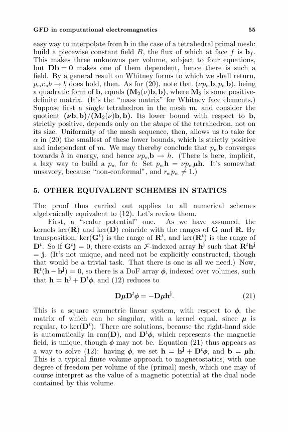
GFD in computational electromagnetics 55
easy way to interpolate from b in the case of a tetrahedral primal mesh:build a piecewise constant field B, the flux of which at face f is bf .This makes three unknowns per volume, subject to four equations,but Db = 0 makes one of them dependent, hence there is such afield. By a general result on Whitney forms to which we shall return,pmrmb → b does hold, then. As for (20), note that (νpmb, pmb), beinga quadratic form of b, equals (M2(ν)b,b), where M2 is some positive-definite matrix. (It’s the “mass matrix” for Whitney face elements.)Suppose first a single tetrahedron in the mesh m, and consider thequotient (ννb,b)/(M2(ν)b,b). Its lower bound with respect to b,strictly positive, depends only on the shape of the tetrahedron, not onits size. Uniformity of the mesh sequence, then, allows us to take forα in (20) the smallest of these lower bounds, which is strictly positiveand independent of m. We may thereby conclude that pmb convergestowards b in energy, and hence νpmb → h. (There is here, implicit,a lazy way to build a pm for h: Set pmh = νpmµµh. It’s somewhatunsavory, because “non-conformal”, and rmpm = 1.)
5. OTHER EQUIVALENT SCHEMES IN STATICS
The proof thus carried out applies to all numerical schemesalgebraically equivalent to (12). Let’s review them.
First, a “scalar potential” one. As we have assumed, thekernels ker(R) and ker(D) coincide with the ranges of G and R. Bytransposition, ker(Gt) is the range of Rt, and ker(Rt) is the range ofDt. So if Gtj = 0, there exists an F-indexed array hj such that Rthj
= j. (It’s not unique, and need not be explicitly constructed, thoughthat would be a trivial task. That there is one is all we need.) Now,Rt(h−hj) = 0, so there is a DoF array φφ, indexed over volumes, suchthat h = hj + Dtφφ, and (12) reduces to
DµµDtφφ = −Dµµhj. (21)
This is a square symmetric linear system, with respect to φφ, thematrix of which can be singular, with a kernel equal, since µµ isregular, to ker(Dt). There are solutions, because the right-hand sideis automatically in ran(D), and Dtφφ, which represents the magneticfield, is unique, though φφ may not be. Equation (21) thus appears asa way to solve (12): having φφ, we set h = hj + Dtφφ, and b = µµh.This is a typical finite volume approach to magnetostatics, with onedegree of freedom per volume of the (primal) mesh, which one may ofcourse interpret as the value of a magnetic potential at the dual nodecontained by this volume.
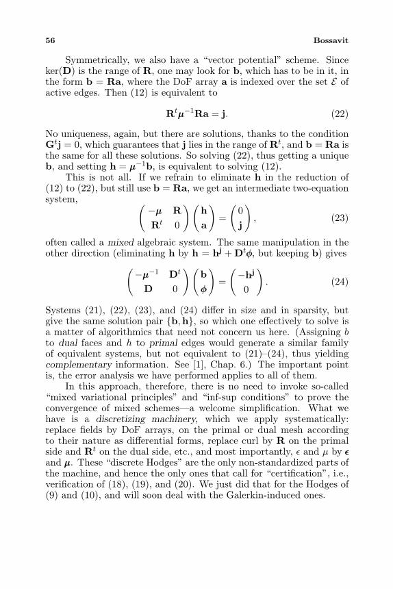
56 Bossavit
Symmetrically, we also have a “vector potential” scheme. Sinceker(D) is the range of R, one may look for b, which has to be in it, inthe form b = Ra, where the DoF array a is indexed over the set E ofactive edges. Then (12) is equivalent to
Rtµµ−1Ra = j. (22)
No uniqueness, again, but there are solutions, thanks to the conditionGtj = 0, which guarantees that j lies in the range of Rt, and b = Ra isthe same for all these solutions. So solving (22), thus getting a uniqueb, and setting h = µµ−1b, is equivalent to solving (12).
This is not all. If we refrain to eliminate h in the reduction of(12) to (22), but still use b = Ra, we get an intermediate two-equationsystem, (
−µµ RRt 0
) (ha
)=
(0j
), (23)
often called a mixed algebraic system. The same manipulation in theother direction (eliminating h by h = hj + Dtφφ, but keeping b) gives
(−µµ−1 Dt
D 0
) (bφφ
)=
(−hj
0
). (24)
Systems (21), (22), (23), and (24) differ in size and in sparsity, butgive the same solution pair b,h, so which one effectively to solve isa matter of algorithmics that need not concern us here. (Assigning bto dual faces and h to primal edges would generate a similar familyof equivalent systems, but not equivalent to (21)–(24), thus yieldingcomplementary information. See [1], Chap. 6.) The important pointis, the error analysis we have performed applies to all of them.
In this approach, therefore, there is no need to invoke so-called“mixed variational principles” and “inf-sup conditions” to prove theconvergence of mixed schemes—a welcome simplification. What wehave is a discretizing machinery, which we apply systematically:replace fields by DoF arrays, on the primal or dual mesh accordingto their nature as differential forms, replace curl by R on the primalside and Rt on the dual side, etc., and most importantly, ε and µ by εεand µµ. These “discrete Hodges” are the only non-standardized parts ofthe machine, and hence the only ones that call for “certification”, i.e.,verification of (18), (19), and (20). We just did that for the Hodges of(9) and (10), and will soon deal with the Galerkin-induced ones.
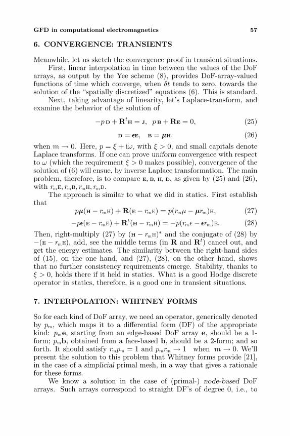
GFD in computational electromagnetics 57
6. CONVERGENCE: TRANSIENTS
Meanwhile, let us sketch the convergence proof in transient situations.First, linear interpolation in time between the values of the DoF
arrays, as output by the Yee scheme (8), provides DoF-array-valuedfunctions of time which converge, when δt tends to zero, towards thesolution of the “spatially discretized” equations (6). This is standard.
Next, taking advantage of linearity, let’s Laplace-transform, andexamine the behavior of the solution of
−pD + RtH = J, pB + RE = 0, (25)
D = εεE, B = µµH, (26)
when m→ 0. Here, p = ξ + iω, with ξ > 0, and small capitals denoteLaplace transforms. If one can prove uniform convergence with respectto ω (which the requirement ξ > 0 makes possible), convergence of thesolution of (6) will ensue, by inverse Laplace transformation. The mainproblem, therefore, is to compare E, B, H, D, as given by (25) and (26),with rme, rmb, rmh, rmd.
The approach is similar to what we did in statics. First establishthat
pµµ(H− rmh) + R(E− rme) = p(rmµ− µµrm)h, (27)
−pεε(E− rme) + Rt(H− rmh) = −p(rmε− εεrm)e. (28)
Then, right-multiply (27) by (H − rmh)∗ and the conjugate of (28) by−(E − rme), add, see the middle terms (in R and Rt) cancel out, andget the energy estimates. The similarity between the right-hand sidesof (15), on the one hand, and (27), (28), on the other hand, showsthat no further consistency requirements emerge. Stability, thanks toξ > 0, holds there if it held in statics. What is a good Hodge discreteoperator in statics, therefore, is a good one in transient situations.
7. INTERPOLATION: WHITNEY FORMS
So for each kind of DoF array, we need an operator, generically denotedby pm, which maps it to a differential form (DF) of the appropriatekind: pme, starting from an edge-based DoF array e, should be a 1-form; pmb, obtained from a face-based b, should be a 2-form; and soforth. It should satisfy rmpm = 1 and pmrm → 1 when m → 0. We’llpresent the solution to this problem that Whitney forms provide [21],in the case of a simplicial primal mesh, in a way that gives a rationalefor these forms.
We know a solution in the case of (primal-) node-based DoFarrays. Such arrays correspond to straight DF’s of degree 0, i.e., to
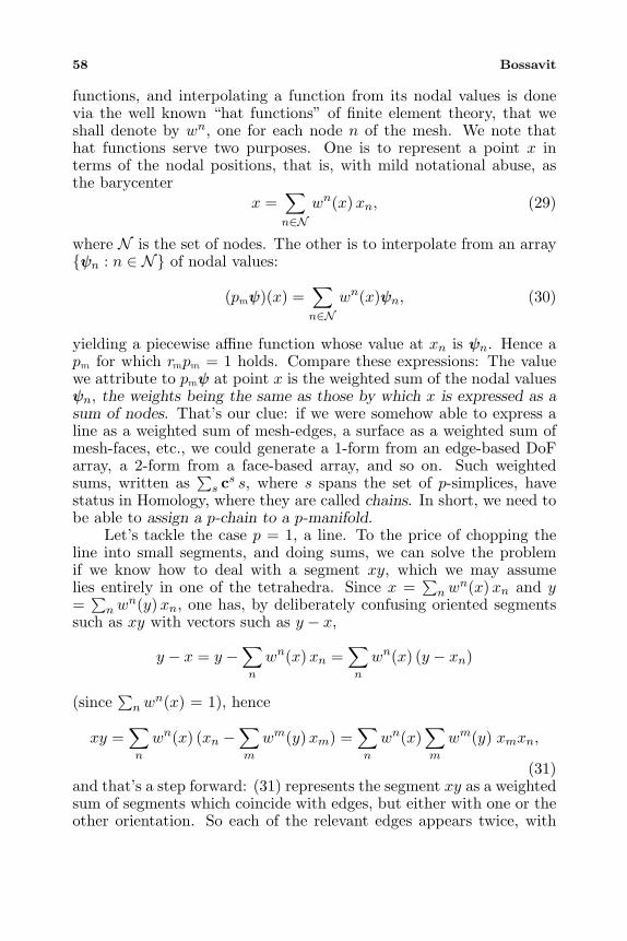
58 Bossavit
functions, and interpolating a function from its nodal values is donevia the well known “hat functions” of finite element theory, that weshall denote by wn, one for each node n of the mesh. We note thathat functions serve two purposes. One is to represent a point x interms of the nodal positions, that is, with mild notational abuse, asthe barycenter
x =∑n∈N
wn(x)xn, (29)
where N is the set of nodes. The other is to interpolate from an arrayψψn : n ∈ N of nodal values:
(pmψψ)(x) =∑n∈N
wn(x)ψψn, (30)
yielding a piecewise affine function whose value at xn is ψψn. Hence apm for which rmpm = 1 holds. Compare these expressions: The valuewe attribute to pmψψ at point x is the weighted sum of the nodal valuesψψn, the weights being the same as those by which x is expressed as asum of nodes. That’s our clue: if we were somehow able to express aline as a weighted sum of mesh-edges, a surface as a weighted sum ofmesh-faces, etc., we could generate a 1-form from an edge-based DoFarray, a 2-form from a face-based array, and so on. Such weightedsums, written as
∑s c
s s, where s spans the set of p-simplices, havestatus in Homology, where they are called chains. In short, we need tobe able to assign a p-chain to a p-manifold.
Let’s tackle the case p = 1, a line. To the price of chopping theline into small segments, and doing sums, we can solve the problemif we know how to deal with a segment xy, which we may assumelies entirely in one of the tetrahedra. Since x =
∑nw
n(x)xn and y=
∑nw
n(y)xn, one has, by deliberately confusing oriented segmentssuch as xy with vectors such as y − x,
y − x = y −∑n
wn(x)xn =∑n
wn(x) (y − xn)
(since∑nw
n(x) = 1), hence
xy =∑n
wn(x) (xn −∑m
wm(y)xm) =∑n
wn(x)∑m
wm(y) xmxn,
(31)and that’s a step forward: (31) represents the segment xy as a weightedsum of segments which coincide with edges, but either with one or theother orientation. So each of the relevant edges appears twice, with
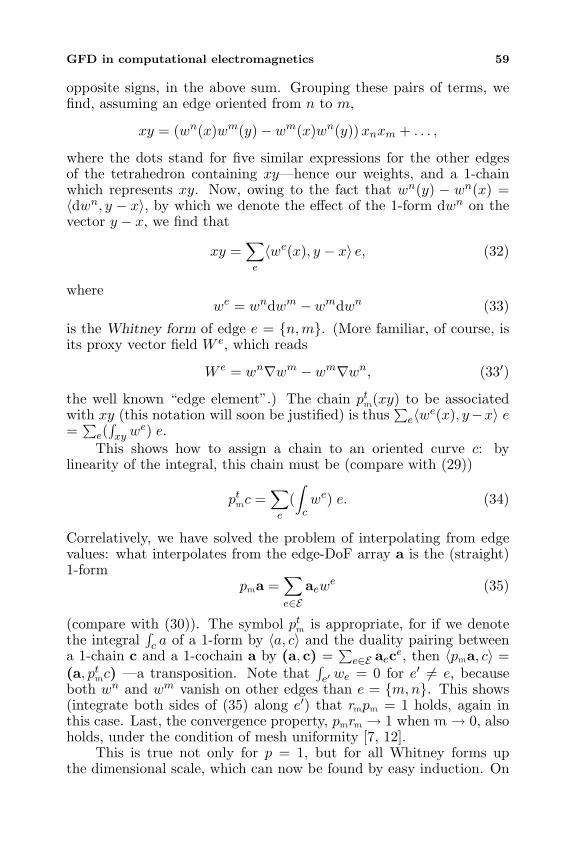
GFD in computational electromagnetics 59
opposite signs, in the above sum. Grouping these pairs of terms, wefind, assuming an edge oriented from n to m,
xy = (wn(x)wm(y)− wm(x)wn(y))xnxm + . . . ,
where the dots stand for five similar expressions for the other edgesof the tetrahedron containing xy—hence our weights, and a 1-chainwhich represents xy. Now, owing to the fact that wn(y) − wn(x) =〈dwn, y − x〉, by which we denote the effect of the 1-form dwn on thevector y − x, we find that
xy =∑e
〈we(x), y − x〉 e, (32)
wherewe = wndwm − wmdwn (33)
is the Whitney form of edge e = n,m. (More familiar, of course, isits proxy vector field W e, which reads
W e = wn∇wm − wm∇wn, (33′)
the well known “edge element”.) The chain ptm(xy) to be associatedwith xy (this notation will soon be justified) is thus
∑e〈we(x), y−x〉 e
=∑e(
∫xy w
e) e.This shows how to assign a chain to an oriented curve c: by
linearity of the integral, this chain must be (compare with (29))
ptmc =∑e
(∫cwe) e. (34)
Correlatively, we have solved the problem of interpolating from edgevalues: what interpolates from the edge-DoF array a is the (straight)1-form
pma =∑e∈E
aewe (35)
(compare with (30)). The symbol ptm is appropriate, for if we denotethe integral
∫c a of a 1-form by 〈a, c〉 and the duality pairing between
a 1-chain c and a 1-cochain a by (a, c) =∑e∈E aece, then 〈pma, c〉 =
(a, ptmc) —a transposition. Note that∫e′ we = 0 for e′ = e, because
both wn and wm vanish on other edges than e = m,n. This shows(integrate both sides of (35) along e′) that rmpm = 1 holds, again inthis case. Last, the convergence property, pmrm → 1 when m→ 0, alsoholds, under the condition of mesh uniformity [7, 12].
This is true not only for p = 1, but for all Whitney forms upthe dimensional scale, which can now be found by easy induction. On
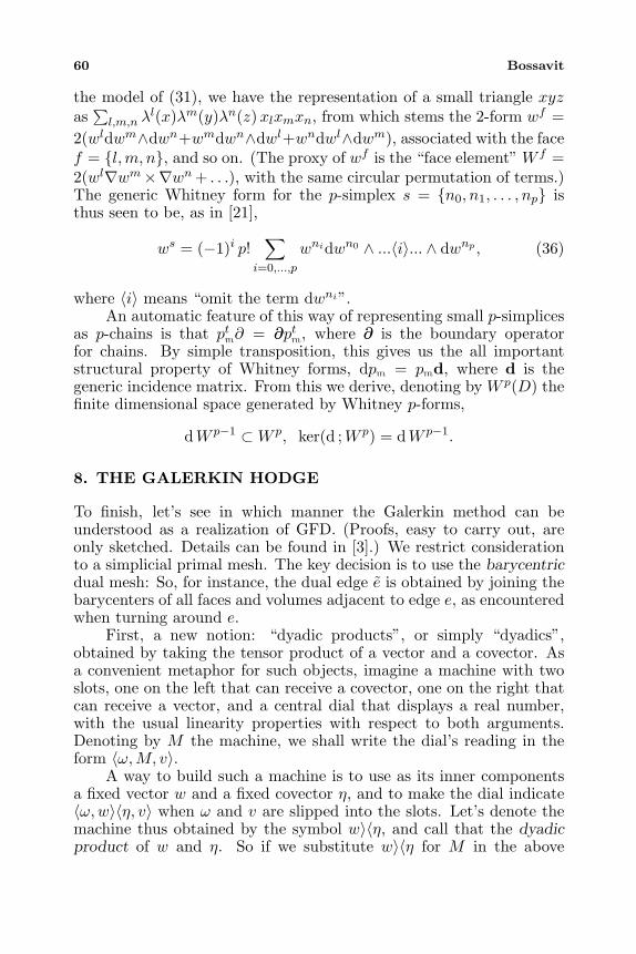
60 Bossavit
the model of (31), we have the representation of a small triangle xyzas
∑l,m,n λ
l(x)λm(y)λn(z)xlxmxn, from which stems the 2-form wf =2(wldwm∧dwn+wmdwn∧dwl+wndwl∧dwm), associated with the facef = l,m, n, and so on. (The proxy of wf is the “face element” W f =2(wl∇wm×∇wn+ . . .), with the same circular permutation of terms.)The generic Whitney form for the p-simplex s = n0, n1, . . . , np isthus seen to be, as in [21],
ws = (−1)i p!∑
i=0,...,p
wnidwn0 ∧ ...〈i〉... ∧ dwnp , (36)
where 〈i〉 means “omit the term dwni”.An automatic feature of this way of representing small p-simplices
as p-chains is that ptm∂ = ∂∂ptm, where ∂∂ is the boundary operatorfor chains. By simple transposition, this gives us the all importantstructural property of Whitney forms, dpm = pmd, where d is thegeneric incidence matrix. From this we derive, denoting by W p(D) thefinite dimensional space generated by Whitney p-forms,
dW p−1 ⊂W p, ker(d ;W p) = dW p−1.
8. THE GALERKIN HODGE
To finish, let’s see in which manner the Galerkin method can beunderstood as a realization of GFD. (Proofs, easy to carry out, areonly sketched. Details can be found in [3].) We restrict considerationto a simplicial primal mesh. The key decision is to use the barycentricdual mesh: So, for instance, the dual edge e is obtained by joining thebarycenters of all faces and volumes adjacent to edge e, as encounteredwhen turning around e.
First, a new notion: “dyadic products”, or simply “dyadics”,obtained by taking the tensor product of a vector and a covector. Asa convenient metaphor for such objects, imagine a machine with twoslots, one on the left that can receive a covector, one on the right thatcan receive a vector, and a central dial that displays a real number,with the usual linearity properties with respect to both arguments.Denoting by M the machine, we shall write the dial’s reading in theform 〈ω,M, v〉.
A way to build such a machine is to use as its inner componentsa fixed vector w and a fixed covector η, and to make the dial indicate〈ω,w〉〈η, v〉 when ω and v are slipped into the slots. Let’s denote themachine thus obtained by the symbol w〉〈η, and call that the dyadicproduct of w and η. So if we substitute w〉〈η for M in the above
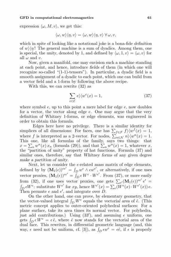
GFD in computational electromagnetics 61
expression 〈ω,M, v〉, we get this:
〈ω,w〉〈η, v〉 = 〈ω,w〉〈η, v〉 ∀ω, v,
which in spite of looking like a notational joke is a bona-fide definitionof w〉〈η ! The general machine is a sum of dyadics. Among them, oneis special, the unity, denoted by 1, and defined by 〈ω, 1, v〉 = 〈ω, v〉 forall ω and v.
Now, given a manifold, one may envision such a machine standingat each point, and hence, introduce fields of them (in which one willrecognize so-called “(1-1)-tensors”). In particular, a dyadic field is asmooth assignment of a dyadic to each point, which one can build froma vector field and a 1-form by following the above recipe.
With this, we can rewrite (32) as∑e∈E
e〉〈we(x) = 1, (37)
where symbol e, up to this point a mere label for edge e, now doublesfor a vector, the vector along edge e. One may argue that the verydefinition of Whitney 1-forms, or edge elements, was engineered inorder to obtain this formula.
Edges here have no privilege. There is a similar identity forsimplices of all dimensions: For faces, one has
∑f∈F f〉〈wf (x) = 1,
where f is interpreted as a 2-vector. For nodes,∑n∈N n〉〈wn(x) = 1.
This one, like all formulas of the family, says two things: thatx =
∑nw
n(x)xn (formula (29)), and that∑nw
n(x) = 1, whatever x,the “partition of unity” property of hat functions. Formula (37) andsimilar ones, therefore, say that Whitney forms of any given degreemake a partition of unity.
Next, let us consider the ε-related mass matrix of edge elements,defined by by (M1(ε))ee
′=
∫D w
e ∧ εwe′ , or alternatively, if one usesvector proxies, (M1(ε))ee
′=
∫D εW
e ·W e′ . From (37), or more easilyfrom (32), if one uses vector proxies, one gets
∑e′(M1(ε))ee
′e′ =∫
D εWe: substitute W e′ for xy, hence W e′(x) =
∑e(W
e(x) ·W e′(x)) e.Then permute e and e′, and integrate over D.
On the other hand, one can prove, by elementary geometry, thatthe vector-valued integral
∫DW
e equals the vectorial area of e. (Thismetric concept applies to outer-oriented polyhedral surfaces: For aplane surface, take its area times its normal vector. For polyhedra,just add contributions.) Using (33′), and assuming ε uniform, onegets
∫D εW
e = ε e, where e now stands for the vectorial area of thedual face. This rewrites, in differential geometric language (and, thisway, ε need not be uniform, cf. [3]), as
∫D εw
e = εe, if ε is properly
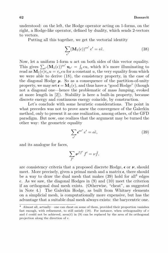
62 Bossavit
understood: on the left, the Hodge operator acting on 1-forms, on theright, a Hodge-like operator, defined by duality, which sends 2-vectorsto vectors.
Putting all this together, we get the vectorial identity∑e′
(M1(ε))ee′e′ = εe. (38)
Now, let a uniform 1-form u act on both sides of this vector equality.This gives
∑e′(M1(ε))ee
′ue′ =
∫e εu, which it’s more illuminating to
read as M1(ε)rmu = rmεu for a constant u, the very equality from whichwe were able to derive (18), the consistency property, in the case ofthe diagonal Hodge µµ. So as a consequence of the partition-of-unityproperty, we may set εε= M1(ε), and thus have a “good Hodge” (thoughnot a diagonal one—hence the problematic of mass lumping, evokedat more length in [2]). Stability is here a built-in property, becausediscrete energy and continuous energy coincide, by construction.
Let’s conclude with some heuristic considerations. The point inwhat precedes was not to prove anew the convergence of the Galerkinmethod, only to present it as one realization, among others, of the GFDparadigm. But now, one realizes that the argument may be turned theother way: the geometric equality
∑e′εεee′e′ = εe, (39)
and its analogue for faces,∑f ′ννff
′f ′ = νf ,
are consistency criteria that a proposed discrete Hodge, εε or νν, shouldmeet. More precisely, given a primal mesh and a matrix εε, there shouldbe a way to draw the dual mesh that makes (39) hold for all4 edgese. As we saw, the diagonal Hodges in (9) and (10) meet the criterionif an orthogonal dual mesh exists. (Otherwise, “cheat”, as suggestedin Note 4.) The Galerkin Hodge, as built from Whitney elementson a simplicial mesh, is computationally more expensive, but has theadvantage that a suitable dual mesh always exists: the barycentric one.4 Almost all, actually—one can cheat on some of them, provided their proportion vanishesfast enough, with refinement, to still satisfy (18). For instance, when orthogonality of eand e could not be achieved, area(e) in (9) can be replaced by the area of its orthogonalprojection along the direction of e.
GFD in computational electromagnetics 63
REFERENCES
1. Bossavit, A., Computational Electromagnetism, Academic Press,Boston, 1998.
2. Bossavit, A. and L. Kettunen, “Yee-like schemes on a tetrahedralmesh, with diagonal lumping,” Int. J. Numer. Modelling, Vol. 12,129–142, 1999.
3. Bossavit, A., “Computational electromagnetism and geometry.(5): The ‘Galerkin hodge’,” J. Japan Soc. Appl. Electromagn. &Mech., 8, Vol. 2, 203–209, 2000.
4. Bossavit, A., “On the notion of anisotropy of constitutivelaws: Some implications of the ‘Hodge implies metric’ result,”COMPEL, to appear.
5. Di Carlo, A. and A. Tiero, “The geometry of linear heat con-duction,” Trends in Applications of Mathematics to Mechanics,W. Schneider, H. Troger, and F. Ziegler (Eds.), 281–287, Long-man, Harlow, 1991.
6. Van Dantzig, D., “The fundamental equations of electromag-netism, independent of metrical geometry,” Proc. Cambridge Phil.Soc., Vol. 30, 421–427, 1934.
7. Dodziuk, J., “Finite-difference approach to the Hodge theory ofharmonic forms,” Amer. J. Math., Vol. 98, No. 1, 79–104, 1976.
8. Hiptmair, R., “Discrete Hodge operators,” this volume.9. Hyman, J. M. and M. Shashkov, “Natural discretizations for the
divergence, gradient, and curl on logically rectangular grids,”Computers Math. Applic., Vol. 33, No. 4, 81–104, 1997.
10. Lee, J.-F. and Z. Sacks, “Whitney elements time domain (WETD)methods,” IEEE Trans. Magn., Vol. 31, No. 3, 1325–1329, 1995.
11. Maxwell, J. C., “On reciprocal figures and diagrams of forces,”Phil. Mag., Series 4, Vol. 27, 250–261, 1864.
12. Muller, W., “Analytic torsion and R-torsion of Riemannianmanifolds,” Advances in Mathematics, Vol. 28, 233–305, 1978.
13. Nicolaides, R. and D.-Q. Wang, “Convergence analysis of acovolume scheme for Maxwell’s equations in three dimensions,”Math. Comp., Vol. 67, 947–963, 1998.
14. Post, E. J., “The constitutive map and some of its ramifications,”Annals of Physics, Vol. 71, 497–518, 1972.
15. Silvester, P. and M. V. K. Chari, “Finite element solution ofsaturable magnetic field problems,” IEEE Trans., PAS-89, Vol. 7,1642–1651, 1970.
16. Taflove, A., Computational Electromagnetics, The Finite Differ-
64 Bossavit
ence in Time Domain Method, Artech House, Boston, London,1995.
17. Teixeira, F. L. and W. C. Chew, “Lattice electromagnetic theoryfrom a topological viewpoint,” J. Math. Phys., Vol. 40, No. 1,169–187, 1999.
18. Tonti, E., “Algebraic topology and computational electromag-netism,” 4th Int. Workshop on Electric and Magnetic Fields, 284–294, A.I.M., Marseilles, 1998.
19. Weiland, T., “Time domain electromagnetic field computationwith finite difference methods,” Int. J. Numer. Modelling, Vol. 9,295–319, 1996.
20. Weiland, T., “Maxwell’s grid equations,” Proc. URSI Int. Symp.Electromagnetic Theory, 37–39, Sydney, Australia, 1992.
21. Whitney, H., Geometric Integration Theory, Princeton U.P.,Princeton, 1957.
22. Yee, K. S., “Numerical solution of initial boundary value problemsinvolving Maxwell’s equations in isotropic media,” IEEE Trans.Ant. & Prop., Vol. 14, No. 3, 302–307, 1966.
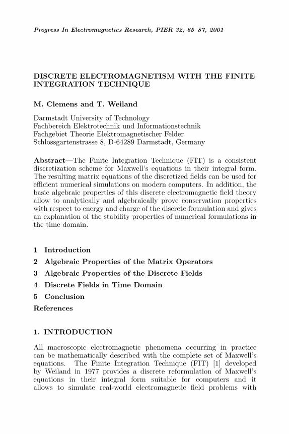
Progress In Electromagnetics Research, PIER 32, 65–87, 2001
DISCRETE ELECTROMAGNETISM WITH THE FINITEINTEGRATION TECHNIQUE
M. Clemens and T. Weiland
Darmstadt University of TechnologyFachbereich Elektrotechnik und InformationstechnikFachgebiet Theorie Elektromagnetischer FelderSchlossgartenstrasse 8, D-64289 Darmstadt, Germany
Abstract—The Finite Integration Technique (FIT) is a consistentdiscretization scheme for Maxwell’s equations in their integral form.The resulting matrix equations of the discretized fields can be used forefficient numerical simulations on modern computers. In addition, thebasic algebraic properties of this discrete electromagnetic field theoryallow to analytically and algebraically prove conservation propertieswith respect to energy and charge of the discrete formulation and givesan explanation of the stability properties of numerical formulations inthe time domain.
1 Introduction
2 Algebraic Properties of the Matrix Operators
3 Algebraic Properties of the Discrete Fields
4 Discrete Fields in Time Domain
5 Conclusion
References
1. INTRODUCTION
All macroscopic electromagnetic phenomena occurring in practicecan be mathematically described with the complete set of Maxwell’sequations. The Finite Integration Technique (FIT) [1] developedby Weiland in 1977 provides a discrete reformulation of Maxwell’sequations in their integral form suitable for computers and itallows to simulate real-world electromagnetic field problems with
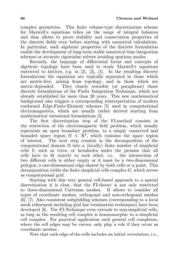
66 Clemens and Weiland
complex geometries. This finite volume-type discretization schemefor Maxwell’s equations relies on the usage of integral balancesand thus allows to prove stability and conservation properties ofthe discrete fields even before starting with numerical calculations.In particular, such algebraic properties of the discrete formulationenable the development of long-term stable numerical time integrationschemes or accurate eigenvalue solvers avoiding spurious modes.
Recently, the language of differential forms and concepts ofalgebraic topology have been used to study Maxwell’s equationsrestricted to lattices, e.g. in [2], [3], [4]. In the resulting discreteformulations the equations are typically separated in those whichare metric-free, arising from topology, and in those which aremetric-depended. They closely resemble (or paraphrase) thosediscrete formulations of the Finite Integration Technique, which arealready established for more than 20 years. This new mathematicalbackground also triggers a corresponding reinterpretation of modernconformal Edge-Finite-Element schemes [5] used in computationalelectromagnetics, which are usually rather derived starting frommathematical variational formulations [3].
The first discretization step of the FI-method consists inthe restriction of the electromagnetic field problem, which usuallyrepresents an open boundary problem, to a simply connected andbounded space region Ω ∈ R3, which contains the space regionof interest. The next step consists in the decomposition of thecomputational domain Ω into a (locally) finite number of simplicialcells Vi such as tetra- or hexahedra under the premise that allcells have to fit exactly to each other, i.e. the intersection oftwo different cells is either empty or it must be a two-dimensionalpolygon, a one-dimensional edge shared by both cells or a point. Thisdecomposition yields the finite simplicial cells complex G, which servesas computational grid.
Starting with this very general cell-based approach to a spatialdiscretization it is clear, that the FI-theory is not only restrictedto three-dimensional Cartesian meshes. It allows to consider alltypes of coordinate meshes, orthogonal and non-orthogonal meshes[6], [7]. Also consistent subgridding schemes (corresponding to a localmesh refinement including grid line termination techniques) have beendeveloped [8]. The FI-Technique even extends to non-simplicial cells,as long as the resulting cell complex is homeomorphic to a simplicialcell complex. For practical application such general cell complexes,where the cell edges may be curves, only play a role if they occur ascoordinate meshes.
Note that each edge of the cells includes an initial orientation, i.e.,
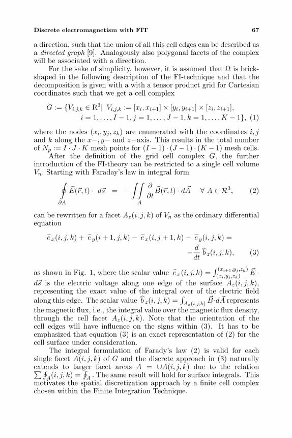
Discrete electromagnetism with FIT 67
a direction, such that the union of all this cell edges can be described asa directed graph [9]. Analogously also polygonal facets of the complexwill be associated with a direction.
For the sake of simplicity, however, it is assumed that Ω is brick-shaped in the following description of the FI-technique and that thedecomposition is given with a with a tensor product grid for Cartesiancoordinates such that we get a cell complex
G := Vi,j,k ∈ R3| Vi,j,k := [xi, xi+1]× [yi, yi+1]× [zi, zi+1],i = 1, . . . , I − 1, j = 1, . . . , J − 1, k = 1, . . . ,K − 1, (1)
where the nodes (xi, yj , zk) are enumerated with the coordinates i, jand k along the x−, y− and z−axis. This results in the total numberof Np := I · J ·K mesh points for (I − 1) · (J − 1) · (K − 1) mesh cells.
After the definition of the grid cell complex G, the furtherintroduction of the FI-theory can be restricted to a single cell volumeVn. Starting with Faraday’s law in integral form∮
∂A
E(r, t) · ds = −∫ ∫
A
∂
∂tB(r, t) · d A ∀ A ∈ R3, (2)
can be rewritten for a facet Az(i, j, k) of Vn as the ordinary differentialequation
e x(i, j, k) +
e y(i + 1, j, k)− e x(i, j + 1, k)−
e y(i, j, k) =
− d
dt
b z(i, j, k), (3)
as shown in Fig. 1, where the scalar value e x(i, j, k) =
∫ (xi+1,yj ,zk)
(xi,yj ,zk)E ·
ds is the electric voltage along one edge of the surface Az(i, j, k),representing the exact value of the integral over of the electric fieldalong this edge. The scalar value
b z(i, j, k) =
∫Az(i,j,k)
B·d A representsthe magnetic flux, i.e., the integral value over the magnetic flux density,through the cell facet Az(i, j, k). Note that the orientation of thecell edges will have influence on the signs within (3). It has to beemphasized that equation (3) is an exact representation of (2) for thecell surface under consideration.
The integral formulation of Farady’s law (2) is valid for eachsingle facet A(i, j, k) of G and the discrete approach in (3) naturallyextends to larger facet areas A = ∪A(i, j, k) due to the relation∑∮
A(i, j, k) =∮A . The same result will hold for surface integrals. This
motivates the spatial discretization approach by a finite cell complexchosen within the Finite Integration Technique.
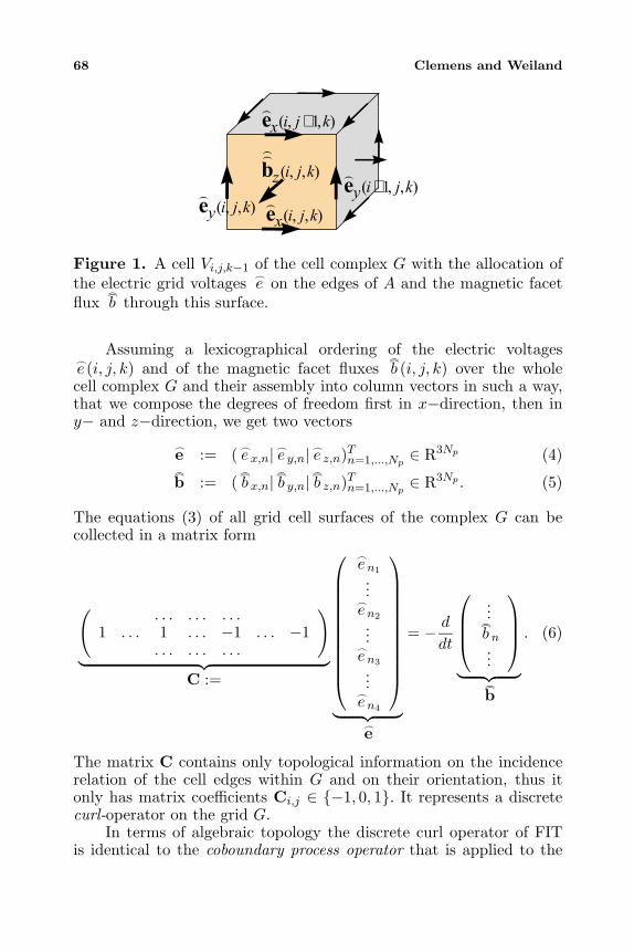
68 Clemens and Weiland
),,( kjiye
),,( kjizb
),1,( kjix e
),,1( kjiy e
),,( kjixe
Figure 1. A cell Vi,j,k−1 of the cell complex G with the allocation ofthe electric grid voltages
e on the edges of A and the magnetic facetflux
b through this surface.
Assuming a lexicographical ordering of the electric voltagese (i, j, k) and of the magnetic facet fluxes
b (i, j, k) over the whole
cell complex G and their assembly into column vectors in such a way,that we compose the degrees of freedom first in x−direction, then iny− and z−direction, we get two vectors
e := (e x,n|e y,n|e z,n)Tn=1,...,Np ∈ R3Np (4)b := (
b x,n|
b y,n|
b z,n)Tn=1,...,Np ∈ R3Np . (5)
The equations (3) of all grid cell surfaces of the complex G can becollected in a matrix form
(. . . . . . . . .
1 . . . 1 . . . −1 . . . −1. . . . . . . . .
)
︸ ︷︷ ︸C :=
en1
...en2
...en3
...en4
︸ ︷︷ ︸e
= − d
dt
...b n...
︸ ︷︷ ︸b
. (6)
The matrix C contains only topological information on the incidencerelation of the cell edges within G and on their orientation, thus itonly has matrix coefficients Ci,j ∈ −1, 0, 1. It represents a discretecurl-operator on the grid G.
In terms of algebraic topology the discrete curl operator of FITis identical to the coboundary process operator that is applied to the
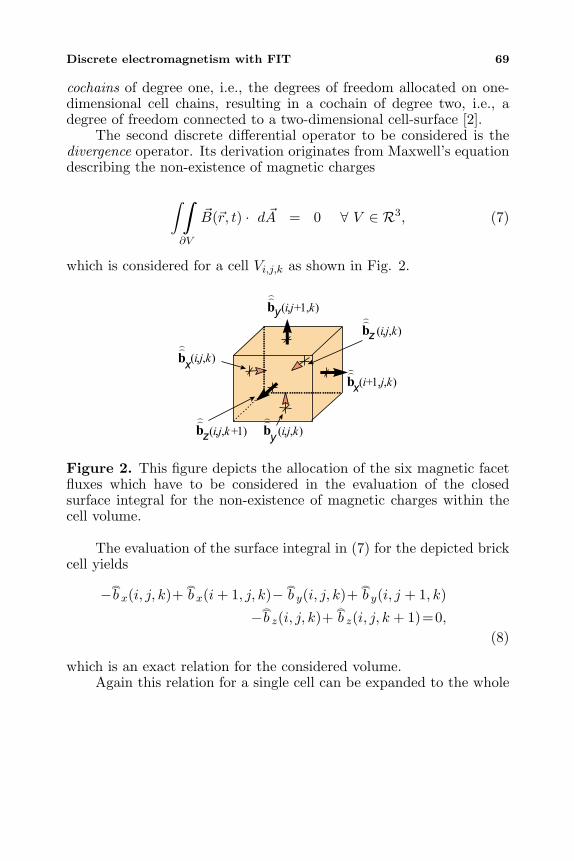
Discrete electromagnetism with FIT 69
cochains of degree one, i.e., the degrees of freedom allocated on one-dimensional cell chains, resulting in a cochain of degree two, i.e., adegree of freedom connected to a two-dimensional cell-surface [2].
The second discrete differential operator to be considered is thedivergence operator. Its derivation originates from Maxwell’s equationdescribing the non-existence of magnetic charges
∫ ∫∫∂V
B(r, t) · d A = 0 ∀ V ∈ R3, (7)
which is considered for a cell Vi,j,k as shown in Fig. 2.
b
y
x
z
z
y
(i+1,j,k)
(i,j,k)
(i,j+1,k)
x(i,j,k)
(i,j,k+1)
(i,j,k)
b
b
b
b
b
Figure 2. This figure depicts the allocation of the six magnetic facetfluxes which have to be considered in the evaluation of the closedsurface integral for the non-existence of magnetic charges within thecell volume.
The evaluation of the surface integral in (7) for the depicted brickcell yields
−b x(i, j, k)+b x(i + 1, j, k)−
b y(i, j, k)+b y(i, j + 1, k)
−b z(i, j, k)+b z(i, j, k + 1)=0,
(8)
which is an exact relation for the considered volume.Again this relation for a single cell can be expanded to the whole
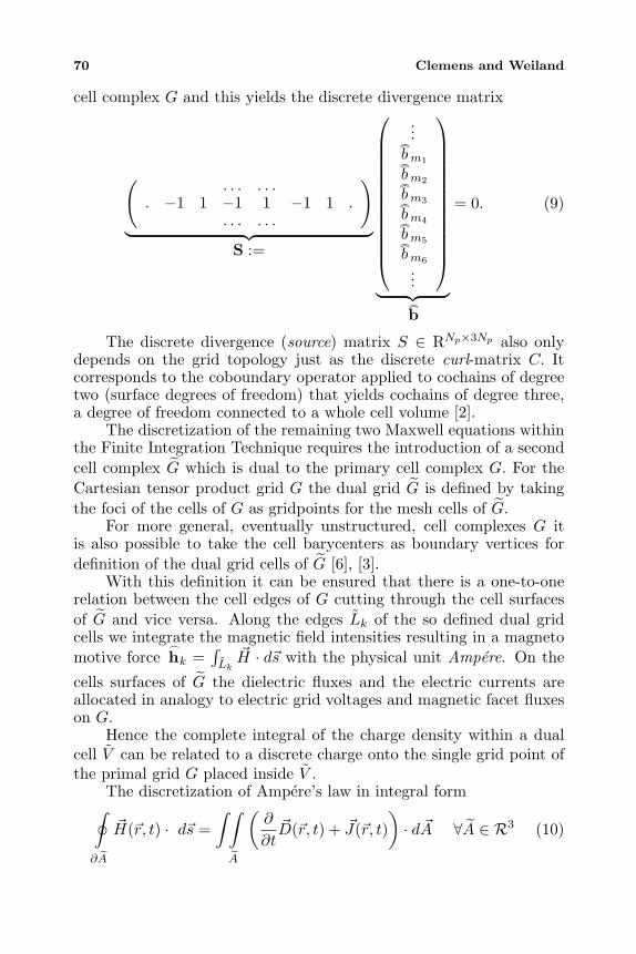
70 Clemens and Weiland
cell complex G and this yields the discrete divergence matrix
(. . . . . .
. −1 1 −1 1 −1 1 .. . . . . .
)
︸ ︷︷ ︸S :=
...bm1bm2bm3bm4bm5bm6
...
︸ ︷︷ ︸b
= 0. (9)
The discrete divergence (source) matrix S ∈ RNp×3Np also onlydepends on the grid topology just as the discrete curl-matrix C. Itcorresponds to the coboundary operator applied to cochains of degreetwo (surface degrees of freedom) that yields cochains of degree three,a degree of freedom connected to a whole cell volume [2].
The discretization of the remaining two Maxwell equations withinthe Finite Integration Technique requires the introduction of a secondcell complex G which is dual to the primary cell complex G. For theCartesian tensor product grid G the dual grid G is defined by takingthe foci of the cells of G as gridpoints for the mesh cells of G.
For more general, eventually unstructured, cell complexes G itis also possible to take the cell barycenters as boundary vertices fordefinition of the dual grid cells of G [6], [3].
With this definition it can be ensured that there is a one-to-onerelation between the cell edges of G cutting through the cell surfacesof G and vice versa. Along the edges Lk of the so defined dual gridcells we integrate the magnetic field intensities resulting in a magnetomotive force
hk =∫Lk
H · ds with the physical unit Ampere. On the
cells surfaces of G the dielectric fluxes and the electric currents areallocated in analogy to electric grid voltages and magnetic facet fluxeson G.
Hence the complete integral of the charge density within a dualcell V can be related to a discrete charge onto the single grid point ofthe primal grid G placed inside V .
The discretization of Ampere’s law in integral form∮
∂A
H(r, t) · ds =∫ ∫
A
(∂
∂tD(r, t) + J(r, t)
)· d A ∀A ∈ R3 (10)
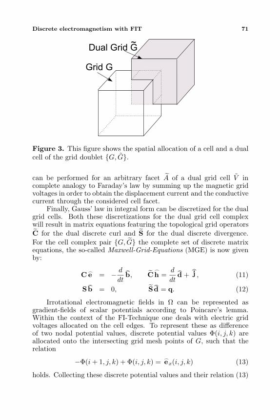
Discrete electromagnetism with FIT 71
Dual Grid G
Grid G
~
Figure 3. This figure shows the spatial allocation of a cell and a dualcell of the grid doublet G, G.
can be performed for an arbitrary facet A of a dual grid cell V incomplete analogy to Faraday’s law by summing up the magnetic gridvoltages in order to obtain the displacement current and the conductivecurrent through the considered cell facet.
Finally, Gauss’ law in integral form can be discretized for the dualgrid cells. Both these discretizations for the dual grid cell complexwill result in matrix equations featuring the topological grid operatorsC for the dual discrete curl and S for the dual discrete divergence.For the cell complex pair G, G the complete set of discrete matrixequations, the so-called Maxwell-Grid-Equations (MGE) is now givenby:
Ce = − d
dt
b, C
h =d
dt
d +
j , (11)
Sb = 0, S
d = q. (12)
Irrotational electromagnetic fields in Ω can be represented asgradient-fields of scalar potentials according to Poincare’s lemma.Within the context of the FI-Technique one deals with electric gridvoltages allocated on the cell edges. To represent these as differenceof two nodal potential values, discrete potential values Φ(i, j, k) areallocated onto the intersecting grid mesh points of G, such that therelation
−Φ(i + 1, j, k) + Φ(i, j, k) = ex(i, j, k) (13)
holds. Collecting these discrete potential values and their relation (13)
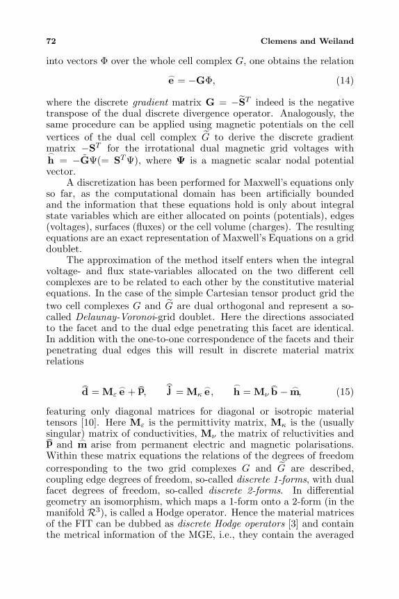
72 Clemens and Weiland
into vectors Φ over the whole cell complex G, one obtains the relatione = −GΦ, (14)
where the discrete gradient matrix G = −ST indeed is the negativetranspose of the dual discrete divergence operator. Analogously, thesame procedure can be applied using magnetic potentials on the cellvertices of the dual cell complex G to derive the discrete gradientmatrix −ST for the irrotational dual magnetic grid voltages with
h = −GΨ(= STΨ), where Ψ is a magnetic scalar nodal potentialvector.
A discretization has been performed for Maxwell’s equations onlyso far, as the computational domain has been artificially boundedand the information that these equations hold is only about integralstate variables which are either allocated on points (potentials), edges(voltages), surfaces (fluxes) or the cell volume (charges). The resultingequations are an exact representation of Maxwell’s Equations on a griddoublet.
The approximation of the method itself enters when the integralvoltage- and flux state-variables allocated on the two different cellcomplexes are to be related to each other by the constitutive materialequations. In the case of the simple Cartesian tensor product grid thetwo cell complexes G and G are dual orthogonal and represent a so-called Delaunay-Voronoi-grid doublet. Here the directions associatedto the facet and to the dual edge penetrating this facet are identical.In addition with the one-to-one correspondence of the facets and theirpenetrating dual edges this will result in discrete material matrixrelations
d = Mε
e +p,
j = Mκ
e ,
h = Mνb − m, (15)
featuring only diagonal matrices for diagonal or isotropic materialtensors [10]. Here Mε is the permittivity matrix, Mκ is the (usuallysingular) matrix of conductivities, Mν the matrix of reluctivities andp and m arise from permanent electric and magnetic polarisations.Within these matrix equations the relations of the degrees of freedomcorresponding to the two grid complexes G and G are described,coupling edge degrees of freedom, so-called discrete 1-forms, with dualfacet degrees of freedom, so-called discrete 2-forms. In differentialgeometry an isomorphism, which maps a 1-form onto a 2-form (in themanifold R3), is called a Hodge operator. Hence the material matricesof the FIT can be dubbed as discrete Hodge operators [3] and containthe metrical information of the MGE, i.e., they contain the averaged
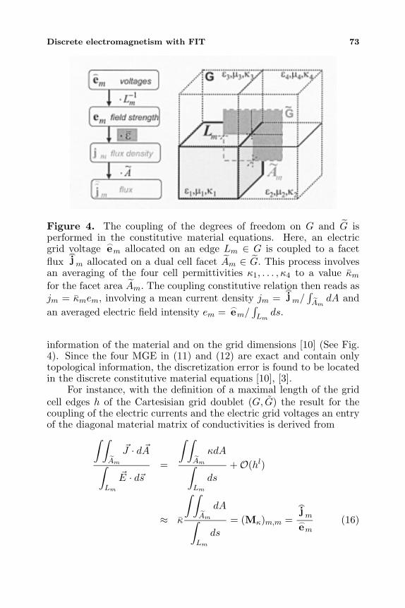
Discrete electromagnetism with FIT 73
Figure 4. The coupling of the degrees of freedom on G and G isperformed in the constitutive material equations. Here, an electricgrid voltage em allocated on an edge Lm ∈ G is coupled to a facetflux
jm allocated on a dual cell facet Am ∈ G. This process involves
an averaging of the four cell permittivities κ1, . . . , κ4 to a value κmfor the facet area Am. The coupling constitutive relation then reads asjm = κmem, involving a mean current density jm =
jm/
∫Am
dA andan averaged electric field intensity em = em/
∫Lm
ds.
information of the material and on the grid dimensions [10] (See Fig.4). Since the four MGE in (11) and (12) are exact and contain onlytopological information, the discretization error is found to be locatedin the discrete constitutive material equations [10], [3].
For instance, with the definition of a maximal length of the gridcell edges h of the Cartesisian grid doublet (G, G) the result for thecoupling of the electric currents and the electric grid voltages an entryof the diagonal material matrix of conductivities is derived from∫ ∫
Am
J · d A∫Lm
E · ds=
∫ ∫Am
κdA
∫Lm
ds
+O(hl)
≈ κ
∫ ∫Am
dA
∫Lm
ds
= (Mκ)m,m =
jmem
(16)
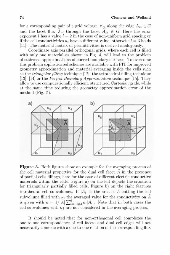
74 Clemens and Weiland
for a corresponding pair of a grid voltage em along the edge Lm ∈ G
and the facet fluxjm through the facet Am ∈ G. Here the error
exponent l has a value l = 2 in the case of non-uniform grid spacing orif the cell conductivities κi have a different value, otherwise l = 3 holds[11]. The material matrix of permittivities is derived analogously.
Coordinate axis parallel orthogonal grids, where each cell is filledwith only one material as shown in Fig. 4, will lead to the problemof staircase approximations of curved boundary surfaces. To overcomethis problem sophisticated schemes are available with FIT for improvedgeometry approximation and material averaging inside the cells suchas the triangular filling technique [12], the tetrahedral filling technique[13], [14] or the Perfect Boundary Approximation technique [15]. Theyallow to use computationally efficient, structured Cartesian grids, whileat the same time reducing the geometry approximation error of themethod (Fig. 5).
Figure 5. Both figures show an example for the averaging process ofthe cell material properties for the dual cell facet A in the presenceof partial cells fillings, here for the case of different electric conductivematerials within the cells. Figure a) on the left depicts the situationfor triangularly partially filled cells, Figure b) on the right featurestetrahedral cell subvolumes. If |Ai| is the area of A cutting the cellsubvolume filled with κi the averaged value for the conductivity on Ais given with κ = 1/|A|∑6
i=1,i=3 κi|Ai|. Note that in both cases thecell subvolumes with κ3 are not considered in the averaging process.
It should be noted that for non-orthogonal cell complexes theone-to-one correspondence of cell facets and dual cell edges will notnecessarily coincide with a one-to-one relation of the corresponding flux
Discrete electromagnetism with FIT 75
and voltage degrees of freedom. The resulting material matrices of theNonorthogonal Finite Integration Technique (N-FIT), are symmetric,but no longer diagonal [7], [16], [17]. A treatment of dispersive,gyrotropic and non-linear material properties within the FI Techniqueresults in numerical schemes which typically concentrate on suitablemodifications of the material matrices [18], [19], [20], [21].
The basic idea for the derivation of the material matrices inFIT, as depicted in Fig. 4, is originally motivated by physicalconsiderations. The derivation of the discrete Hodges operators forEdge-Finite-Element schemes, however, with their origin in variationalformulations, involves the element-by-element quadrature of theWhitney edge shape functions we [22], given here e.g. for the massmatrix of conductivities on a tetrahedral element grid with
(Mκ)FEi,j =
∫Aκwei · wej dA. (17)
As in the N-FIT case, the resultant material matrices of thediscrete constitutive equations will be symmetric (and eventually badlyconditioned for obtuse edge angles) and non-diagonal. An artificial re-diagonalization of these matrices with so-called lumping techniques isexplained in [22] for tetrahedral meshes.
2. ALGEBRAIC PROPERTIES OF THE MATRIXOPERATORS
One of the essential properties of the discrete representation ofMaxwell’s equations by the boundary path and surface integralapproach (hence Finite Integration) lies in the discrete analog to thevectoranalytical equation
div curl = 0, (18)
given with the matrix equations
SC = 0, (19)
SC = 0, (20)
for the cell complex doublet G, G. These relations result from thefact, that for all grid cells the calculation of the discrete divergenceS consists in the summation of the flux components. For these fluxcomponents any grid voltage (left-multiplied with the discrete curl-matrix C) is each considered twice with different sign in the curl-summation giving the zero divergence result of the overall summation
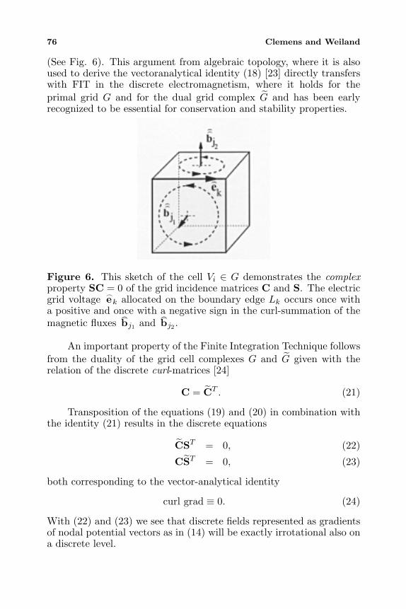
76 Clemens and Weiland
(See Fig. 6). This argument from algebraic topology, where it is alsoused to derive the vectoranalytical identity (18) [23] directly transferswith FIT in the discrete electromagnetism, where it holds for theprimal grid G and for the dual grid complex G and has been earlyrecognized to be essential for conservation and stability properties.
Figure 6. This sketch of the cell Vi ∈ G demonstrates the complexproperty SC = 0 of the grid incidence matrices C and S. The electricgrid voltage ek allocated on the boundary edge Lk occurs once witha positive and once with a negative sign in the curl-summation of themagnetic fluxes
bj1 and
bj2 .
An important property of the Finite Integration Technique followsfrom the duality of the grid cell complexes G and G given with therelation of the discrete curl-matrices [24]
C = CT . (21)
Transposition of the equations (19) and (20) in combination withthe identity (21) results in the discrete equations
CST = 0, (22)
CST = 0, (23)
both corresponding to the vector-analytical identity
curl grad ≡ 0. (24)
With (22) and (23) we see that discrete fields represented as gradientsof nodal potential vectors as in (14) will be exactly irrotational also ona discrete level.
Discrete electromagnetism with FIT 77
The matrix equations (19), (20), (22) and (23) include only theincidence relations of the grid topology and do not contain any metricalnotions [25]. They represent the typical so-called complex property ofthe simplicial grid cell complex [23]. The background mathematicalconnection between the discrete matrix identities (19)–(23) to thevectoranalytical identities (18) and (24) becomes readily available,when the degrees of freedom in the Finite Integration Technique areconsidered as discrete differential forms in which case the discrete gridtopology matrix operators have the same effect as Cartan’s differentialoperator, which yields the vector-analytical operators curl, grad,div(Cf. [2]).
3. ALGEBRAIC PROPERTIES OF THE DISCRETEFIELDS
With the complex properties (19)–(23) and relation (21) arising fromthe duality of the dual grid doublet G, G important existence anduniqueness results can be derived for the discrete grid fields by simplyapplying theoretical results from linear algebra.
An important feature of the FI-Technique as spatial discretizationscheme for Maxwell’s equations is the build-in continuity equation
S(C
h) = S(
d
dt
d +
j)
= 0, (25)
which corresponds to the analytic continuity equation
div(
∂
∂tD + J
)= 0⇐⇒ d
dtq + S
j = 0. (26)
The discrete continuity equation ensures that no spurious chargeswill occur. Such non-physical charges would result in static fieldscontaminating discrete transient field solutions.
If electromagnetic field processes are calculated in time domain,energy conservation of the time and space discrete system becomesof paramount importance. If this condition is violated, a necessaryprerequisite for a long-term stable time integration of electromagneticwave-propagation phenomena without artificial numerical damping isnot available. For the FI-Technique the proof of this condition wasgiven in [24], [26] for resonator structures with perfectly conductingwalls.
The transformation into frequency domain for the Maxwell-Grid-Equations in (11) with e(t) = Re(eeiωt) for a situation without lossy
78 Clemens and Weiland
materials (Mκ = 0) and without external current excitation (je = 0)
yields
Ce = −iω b, (27)
CMνb = +iω Mε
e . (28)
Combining these equations a general real-valued algebraic eigenvalueproblem is obtained with the homogeneous curlcurl equation
CMνCe = ω2 Mε
e . (29)
Additional normalization with e , := M1/2ε
e of equation (29) resultsin a typical real-valued eigenvalue problem
(M1/2ν CM−1/2
ε )T (M1/2ν CM−1/2
ε )e , = ω2 e ,. (30)
With the additional assumption of symmetric and positive definitematerial matrices Mν and Mε, the symmetry of this algebraiceigenvalue problem directly yields that all eigenvalues ω2 of the curl-curl system matrix have to be real-valued and nonnegative. Thus adiscrete field solution in time domain, which can always be decomposedinto a linear combination of such undamped loss-free eigensolutions,will neither grow nor decay in time.
Another important property of the curlcurl equation withoutlosses becomes apparent by left-multiplication of the discretedivergence matrix S
SCMνCe = ω2 SMε
e . (31)
Due to relation (20) of the grid incidence matrices the equation
ω2 SMεe = 0, (32)
is obtained. In case of singly connected metallic boundaries of thecomputational domain (32) allows the two possible solutions for thedielectric facet fluxes
d = Mε
e [27], [24]:
d :
ω2 = 0 : S
d = 0
ω2 = 0 : Sd = 0
. (33)
For situations in which the boundaries of perfectly electrically con-ductive regions of the computational domain are not singly connected,there are also non-trivial solutions
d for which both S
d = 0 and
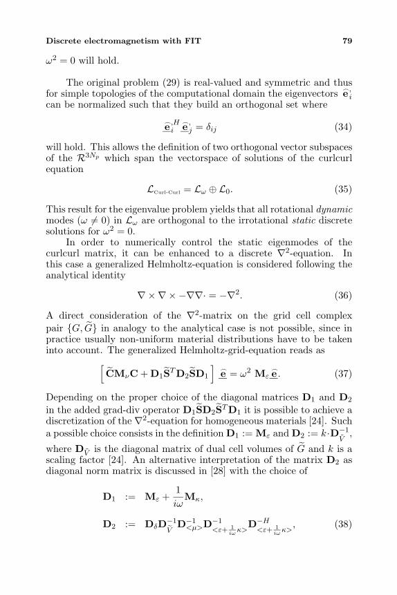
Discrete electromagnetism with FIT 79
ω2 = 0 will hold.
The original problem (29) is real-valued and symmetric and thusfor simple topologies of the computational domain the eigenvectors e ,
ican be normalized such that they build an orthogonal set where
e ,Hi
e ,j = δij (34)
will hold. This allows the definition of two orthogonal vector subspacesof the R3Np which span the vectorspace of solutions of the curlcurlequation
LCurl-Curl = Lω ⊕ L0. (35)
This result for the eigenvalue problem yields that all rotational dynamicmodes (ω = 0) in Lω are orthogonal to the irrotational static discretesolutions for ω2 = 0.
In order to numerically control the static eigenmodes of thecurlcurl matrix, it can be enhanced to a discrete ∇2-equation. Inthis case a generalized Helmholtz-equation is considered following theanalytical identity
∇×∇×−∇∇· = −∇2. (36)
A direct consideration of the ∇2-matrix on the grid cell complexpair G, G in analogy to the analytical case is not possible, since inpractice usually non-uniform material distributions have to be takeninto account. The generalized Helmholtz-grid-equation reads as
[CMνC + D1STD2SD1
]e = ω2 Mε
e . (37)
Depending on the proper choice of the diagonal matrices D1 and D2
in the added grad-div operator D1SD2STD1 it is possible to achieve adiscretization of the ∇2-equation for homogeneous materials [24]. Sucha possible choice consists in the definition D1 := Mε and D2 := k·D−1
V,
where DV is the diagonal matrix of dual cell volumes of G and k is ascaling factor [24]. An alternative interpretation of the matrix D2 asdiagonal norm matrix is discussed in [28] with the choice of
D1 := Mε +1iω
Mκ,
D2 := DδD−1
VD−1
<µ>D−1<ε+ 1
iωκ>
D−H<ε+ 1
iωκ>
, (38)
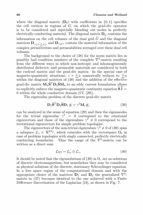
80 Clemens and Weiland
where the diagonal matrix (Dδ) with coefficients in 0, 1 specifiesthe cell vertices in regions of G, on which the grad-div operatoris to be considered and especially blending out nodes in perfectlyelectrically conducting material. The diagonal matrix DV contains theinformation on the cell volumes of the dual grid G and the diagonalmatrices D<ε+ 1
iωκ> and D<µ> contain the material information of the
complex permittivities and permeabilities averaged over these dual cellvolumes.
The background to the choice of (38) for the norm matrix lies inpossibly bad condition numbers of the complete ∇2-matrix resultingfrom the different ways in which non-isotropic and inhomogeneouslydistributed dielectric und permeable materials are considered in boththe curlcurl matrix and the grad-div matrix. In the special case ofmagneto-quasistatic situations, ε + 1
iωκ numerically reduces to 1iωκ
within the diagonal matrices of (38) and the addition of the effectivegrad-div matrix MκSTD2SMκ to an eddy current formulation allowsto explicitly enforce the magneto-quasistatic continuity equation S
j =
0 within the whole conductive domain (Cf. [29]).The eigenvalue problem of the discrete grad-div matrix
D1STD2SD1e = γ2Mε
e , (39)
can be analyzed in the sense of equation (29) and then the eigenmodesfor the trivial eigenvalue γ2 = 0 correspond to the rotationaleigenvectors and those of the eigenvalues γ2 = 0 correspond to theirrotational eigenvectors for simple problem topologies.
The eigenvectors of the non-trivial eigenvalues γ2 = 0 of (39) spana subspace Lγ ∈ R3Np , which coincides with the vectorspace Ω0 incase of problem topologies with singly connected, perfectly electricallyconducting boundaries. Thus the range of the ∇2-matrix can bewritten as a direct sum
L∇2 = Lω ⊕ Lγ . (40)
It should be noted that the eigensolutions of (39) in Ωγ are no solutionsof discrete electromagnetism, but nonetheless they may be consideredas physical solutions of the discrete, stationary Schroedinger equation.In a free space region of the computational domain and with theappropriate choice of the matrices D1 and D2 the generalized ∇2-matrix in (37) becomes identical to the one achieved with a FiniteDifference discretization of the Laplacian [24], as shown in Fig. 7.
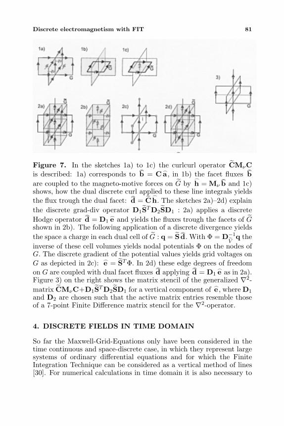
Discrete electromagnetism with FIT 81
Figure 7. In the sketches 1a) to 1c) the curlcurl operator CMνCis described: 1a) corresponds to
b = Ca , in 1b) the facet fluxes
b
are coupled to the magneto-motive forces on G by
h = Mνb and 1c)
shows, how the dual discrete curl applied to these line integrals yieldsthe flux trough the dual facet:
d = C
h. The sketches 2a)–2d) explainthe discrete grad-div operator D1STD2SD1 : 2a) applies a discreteHodge operator
d = D1
e and yields the fluxes trough the facets of Gshown in 2b). The following application of a discrete divergence yieldsthe space a charge in each dual cell of G : q = S
d. With Φ = D−1
Vq the
inverse of these cell volumes yields nodal potentials Φ on the nodes ofG. The discrete gradient of the potential values yields grid voltages onG as depicted in 2c): e = STΦ. In 2d) these edge degrees of freedomon G are coupled with dual facet fluxes
d applying
d = D1
e as in 2a).Figure 3) on the right shows the matrix stencil of the generalized ∇2-matrix CMνC+D1STD2SD1 for a vertical component of e , where D1
and D2 are chosen such that the active matrix entries resemble thoseof a 7-point Finite Difference matrix stencil for the ∇2-operator.
4. DISCRETE FIELDS IN TIME DOMAIN
So far the Maxwell-Grid-Equations only have been considered in thetime continuous and space-discrete case, in which they represent largesystems of ordinary differential equations and for which the FiniteIntegration Technique can be considered as a vertical method of lines[30]. For numerical calculations in time domain it is also necessary to
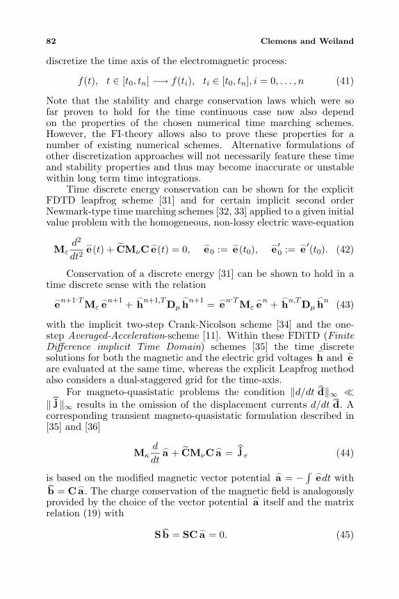
82 Clemens and Weiland
discretize the time axis of the electromagnetic process:
f(t), t ∈ [t0, tn] −→ f(ti), ti ∈ [t0, tn], i = 0, . . . , n (41)
Note that the stability and charge conservation laws which were sofar proven to hold for the time continuous case now also dependon the properties of the chosen numerical time marching schemes.However, the FI-theory allows also to prove these properties for anumber of existing numerical schemes. Alternative formulations ofother discretization approaches will not necessarily feature these timeand stability properties and thus may become inaccurate or unstablewithin long term time integrations.
Time discrete energy conservation can be shown for the explicitFDTD leapfrog scheme [31] and for certain implicit second orderNewmark-type time marching schemes [32, 33] applied to a given initialvalue problem with the homogeneous, non-lossy electric wave-equation
Mεd2
dt2e(t) + CMνC
e(t) = 0, e0 := e(t0),e ′0 := e ′(t0). (42)
Conservation of a discrete energy [31] can be shown to hold in atime discrete sense with the relationen+1,TMε
en+1 +
hn+1,TDµ
hn+1 = en,TMεen +
hn,TDµ
hn (43)
with the implicit two-step Crank-Nicolson scheme [34] and the one-step Averaged-Acceleration-scheme [11]. Within these FDiTD (FiniteDifference implicit Time Domain) schemes [35] the time discretesolutions for both the magnetic and the electric grid voltages
h and eare evaluated at the same time, whereas the explicit Leapfrog methodalso considers a dual-staggered grid for the time-axis.
For magneto-quasistatic problems the condition ‖d/dt d‖∞ ‖j ‖∞ results in the omission of the displacement currents d/dt
d. A
corresponding transient magneto-quasistatic formulation described in[35] and [36]
Mκd
dta + CMνC
a =j e (44)
is based on the modified magnetic vector potential a = −∫ edt with
b = Ca . The charge conservation of the magnetic field is analogouslyprovided by the choice of the vector potential a itself and the matrixrelation (19) with
Sb = SCa = 0. (45)
Discrete electromagnetism with FIT 83
The discrete magneto-quasistatic continuity equation (25) reduces toSj = 0, corresponding to Kirchhoff’s law of a zero current balance
at nodes of electrical circuits, if one artificially restricts the currentsallocated on the dual cell facets to the corresponding one-dimensionaledges of the primary grid.
Thus external excitation currentsj e must be of vanishing
divergence, which is the case for excitation coils with closed loops orstationary current fields modelled in G. This also prohibits the use ofantennas as excitation sources within these formulations, since discretecharges would have to be considered at their ends. In addition, in theconducting regions this magneto-quasistatic continuity equation S
j =
−SMκddt
a = 0 corresponds to a gauging of the vector potential, whichtakes into account possible jumps in the components of the vectorpotential normal to interfaces of materials with different conductivity.A time discretization of the non-gauged transient magneto-quasistaticformulation (44) with a θ-one-step method [33] yields a consistentlysingular system of equations[
1θ∆t
Mκ + CMνC]an+1 =
[1
θ∆tMκ +
1− θ
θCMνC
]an +
j n+1e +
1− θ
θ
j ne , (46)
which have to be solved repeatedly. Nonlinear ferromagnetic materialbehaviour modelled in Mν(
an+1) can be tackled with linearizationtechniques and the resulting linear systems will have a similar structureto (46) [37]. Left multiplication of (46) with S shows that the continuityequation for the eddy currents will be enforced in a time discretizedsense with
SMκan+1 = SMκ
an = . . . = SMκa0
. (47)
Note, that for the magneto-quasistatic formulation with its continuityequation S
j = 0 also the condition d/dtq = 0 is implied from
the discrete continuity condition of the complete set of Maxwell-Grid-Equations. The result d/dtq = 0 provides, that no spuriousirrotational solution parts will accumulate in a in the non-conductiveregions arising from the spatial discretization itself. If in additiona solution method for the consistently singular system (46) with aweak gauging property, as featured by e.g. the conjugate gradientmethod [35], is applied with a zero start vector of the iteration, therelation SDan+1 = 0 will hold for exact arithmetics. Thus the chargeconservation property of the FI Technique also becomes an integralpart of the non-gauged formulation (44) itself.
84 Clemens and Weiland
5. CONCLUSION
The Finite Integration Technique is a discretization method whichtransforms Maxwell’s equations onto a dual grid cell complex, resultingin a set of discrete matrix equations. The degrees of freedomcollected in the vectors of this discretization scheme, typically consist inphysically measurable, integral quantities such as voltages, currents orcharges. This discretization approach results in sparse integer matricesC, C,S, S which only contain information on the incidence relations ofthe dual cell complex. This mere restriction to topological informationof the simplicial grid is responsible for the typical complex propertySC = 0 and SC = 0. In connection with the relation C = CT
due to the duality of the grid pair and with symmetric and positivedefinite material matrices the topologically related relations of theseincidence matrices allow to prove energy and charge conservation ofthe spatially discretized formulations. For the homogenous undampedcurlcurl equation a real-valued spectrum with orthogonal subspaces forstatic and dynamic eigenmodes was shown to exist. In addition, thealgebraic properties of the MGE of FIT also allow to prove charge andenergy conservation within time discrete schemes such as the explicitLeapfrog FDTD scheme or certain second order implicit methods.Implicit time integration schemes can also be applied to non-gaugedmagneto-quasistatic formulations, which yield singular matrix systemsthat still can be numerically tackled due to their consistency givenwith the FIT approach. These results clearly distinguish these timeintegration schemes from many alternative methods which do notrely on space and time stability and thus may become unstable orinaccurate within long term calculations.
REFERENCES
1. Weiland, T., “A discretization method for the solution ofMaxwell’s equations for six-component fields,” Electronics andCommunications AEU, Vol. 31, No. 3, 116–120, 1977.
2. Tonti, E., “On the geometrical structure of electromag-netism,” Gravitation, Electromagnetism and Geometrical Struc-tures, G. Ferraese (ed.), 281–308, Pitagora, Bologna, 1996.
3. Bossavit, A., L. Kettunen, and T. Tarhassaari, “Some realizationsof a discrete Hodge operator: A reinterpretation of the finiteelement technique,” IEEE Transactions on Magnetics, Vol. 35,1494–1497, May 1999.
4. Teixeira, F. L. and W. C. Chew, “Lattice electromagnetic theory
Discrete electromagnetism with FIT 85
from a topological viewpoint,” Journal of Mathematical Physics,Vol. 40, No. 1, 169–187, 1999.
5. Nedelec, J. C., “Mixed finite elements in R3,” NumerischeMathematik, No. 35, 315–341, 1980.
6. van Rienen, U. and T. Weiland, “Triangular discretization methodfor the evaluation of RF-fields in cylindrically symmetric cavities,”IEEE Transactions on Magnetics, Vol. MAG-21, No. 6, 2317–2320, 1985.
7. Schuhmann, R. and T. Weiland, “A stable interpolation techniquefor FDTD on nonorthogonal grids,” International Journal onNumerical Modelling, Vol. 11, 299–306, May 1998.
8. Thoma, P. and T. Weiland, “A consistent subgridding scheme forthe finite difference time domain method,” International Journalof Numerical Modelling, Vol. 9, 359–374, 1996.
9. Chen, W. K., Graph Theory and It’s Engineering Applications,Vol. 5, Advanced Series in Electrical and Computer Engineering,World Scientific, Singapor, 1996.
10. Weiland, T., “Time domain electromagnetic field computationwith finite difference methods,” International Journal of Numer-ical Modelling: Electronic Networks, Devices and Fields, Vol. 9,259–319, 1996.
11. Clemens, M., “Zur numerischen Berechnung zeitlich langsam-veranderlicher elektromagnetischer Felder mit der Finiten-Integrations-Methode,” Ph.D. thesis, Technische UniversitatDarmstadt, 1998.
12. Weiland, T., “Lossy waveguides with arbitrary boundary contourand distribution of material,” Electronics and CommunicationsAEU, Vol. 33, 170, 1979.
13. Muller, W. and W. Wolff, “Ein Beitrag zur numerischenBerechnung von Magnetfeldern,” Elektrotechnische Zeitung,Vol. 96, 269–273, 1975.
14. Muller, W., J. Kruger, A. Jacobus, R. Winz, T. Weiland, H. Euler,U. Kamm, and W. R. Novender, “Numerical solution of 2- and 3-dimensional nonlinear field problems by means of the computerprogram PROFI,” Archiv fur Elektrotechnik, Vol. 65, 299–307,1982.
15. Krietenstein, B., P. Thoma, R. Schuhmann, and T. Weiland, “Theperfect boundary approximation technique facing the big challengeof high precision computation,” Proceedings of the 19th LINACConference, Chicago, August 1998.
16. Schuhmann, R. and T. Weiland, “FDTD on nonorthogonal
86 Clemens and Weiland
grids with triangular fillings,” IEEE Transactions on Magnetics,Vol. 35, 1470–1473, May 1999.
17. Clemens, M., M. Hilgner, R. Schuhmann, and T. Weiland,“Transient eddy current simulation using the nonorthogonal finiteintegration technique,” Conference Records of the CEFC 2000,Milwaukee, 385, 2000. Full paper submitted to IEEE Transactionson Magnetics.
18. Gutschling, S., “Zeitbereichsverfahren zur simulation elektromag-netischer felder in dispersiven materialien,” Ph.D. thesis, Tech-nische Universitat Darmstadt, 1998.
19. Gutschling, S., H. Kruger, H. Spachmann, and T. Weiland, “FIT-formulation for nonlinear dispersive media,” International Journalon Numerical Modelling, Vol. 12, 81–92, 1999.
20. Kruger, H., H. Spachmann, and T. Weiland, “FIT-formulation forgyrotropic media,” Proceedings of the ICCEA1999, Torino, Italy,1999.
21. Clemens, M., S. Drobny, and T. Weiland, “Time integrationof slowly-varying electromagnetic field problems using the finiteintegration technique,” Proceedings of the ENUMATH 97, 246–253, Heidelberg, 1999.
22. Bossavit, A. and L. Kettunen, “Yee-like schemes on a tetrahedralmesh, with diagonal lumping,” International Journal of NumericalModelling: Electronic Networks, Devices and Fields, Vol. 12,No. 1/2, 129–142, 1999.
23. Janich, K., Vektoranalysis, 191–222, Springer Lehrbuch, Springer,1993.
24. Weiland, T., “On the unique numerical solution of Maxwellianeigenvalue problems in three dimensions,” Particle Accelerators,Vol. 17, 227–242, 1985.
25. Tonti, E., “Discrete formulation of the electromagnetic field,”University Trieste, 34127 Trieste, Italy, 1998.
26. Thoma, P. and T. Weiland, “Numerical stability of finitedifference time domain methods,” IEEE Transactions onMagnetics, Vol. 34, No. 5, 2740–2743, 1998.
27. Schmitt, D., “Zur numerischen berechnung von resonatoren undwellenleitern,” Ph.D. thesis, Technische Hochschule Darmstadt,1994.
28. Hahne, P., “Zur numerischen berechnung zeitharmonischer elek-tromagnetischer felder,” Ph.D. thesis, Technische HochschuleDarmstadt, 1992.
29. Bossavit, A., “‘stiff’ problems in eddy-current theory and the
Discrete electromagnetism with FIT 87
regularization of Maxell’s equations,” in Conference Records ofthe CEFC 2000, Milwaukee, 497, 1997. Full paper submitted toIEEE Transactions on Magnetics.
30. Grosmann, C. and H.-G. Roos, Numerik partieller Differentialgle-ichungen, B. G. Teubner Verlag, Stuttgart, 1994.
31. Schuhmann, R. and T. Weiland, “Conservation of discrete energyand related laws in the finite integration technique,” this volume.
32. Zienkiewicz, O. C., “A new look at the Newmark, Houbolt andother time stepping formulas. A weighted residual approach,”Earthquake Engineering and Structural Dynamics, No. 5, 413–418,1977.
33. Zienkiewicz, O. C., W. L. Wood, N. H. Hine, and R. L. Taylor,“A unified set of single step algorithms; part 1,” Int. J. for Num.Meth. in Eng., Vol. 20, 1529–1552, 1984.
34. Monk, P., “A mixed method for approximating Maxwell’sequations,” SIAM J. Numer. Anal., Vol. 28, 1610–1634, December1991.
35. Clemens, M. and T. Weiland, “Transient eddy current calculationwith the FI-method,” IEEE Transactions on Magnetics, Vol. 35,1163–1166, May 1999.
36. Clemens, M. and T. Weiland, “Numerical algorithms for theFDiTD and FDFD simulation of slowly-varying electromagneticfields,” Int. J. Numerical Modelling, Special Issue on FiniteDifference Time Domain and Frequency Domain Methods, Vol. 12,No. 1/2, 3–22, 1999.
37. Drobny, S., M. Clemens, and T. Weiland, “Dual nonlinearmagnetostatic formulations using the finite integration technique,”Conference Records of the CEFC 2000, Milwaukee, 392, 2000. Fullpaper submitted to IEEE Transactions on Magnetics.
Progress In Electromagnetics Research, PIER 32, 89–121, 2001
MIMETIC FINITE DIFFERENCE METHODS FORMAXWELL’S EQUATIONS AND THE EQUATIONS OFMAGNETIC DIFFUSION
J. M. Hyman and M. Shashkov
Los Alamos National LaboratoryT-7, MS-B284Los Alamos NM 87545, USA
Abstract—We have constructed mimetic finite difference methodsfor both the TE and TM modes for 2-D Maxwell’s curl equationsand equations of magnetic diffusion with discontinuous coefficientson nonorthogonal, nonsmooth grids. The discrete operators werederived using the discrete vector and tensor analysis to satisfy discreteanalogs of the main theorems of vector analysis. Because the finitedifference methods satisfy these theorems, they do not have spurioussolutions and the “divergence-free” conditions for Maxwell’s equationsare automatically satisfied. The tangential components of the electricfield and the normal components of magnetic flux used in the FDMare continuous even across discontinuities. This choice guaranteesthat problems with strongly discontinuous coefficients are treatedproperly. Furthermore on rectangular grids the method reduces tothe analytically correct averaging for discontinuous coefficients. Weverify that the convergence rate was between first and second orderon the arbitrary quadrilateral grids and demonstrate robustness of themethod in numerical examples.
1 Introduction and Background
2 Discrete Function Spaces and Inner Products2.1 Discrete Scalar and Vector Functions2.2 Discrete Inner Products
2.2.1 The Dot Product2.2.2 Formal Inner Products2.2.3 Natural Inner Products2.2.4 Inner Product Identities
90 Hyman and Shashkov
3 Discretization of the Curl Operators3.1 Discretization of curl E3.2 Discretization of ε−1 curlµ−1 B
4 Discretization of the Divergence and Gradient4.1 Discretization of div B
4.2 Discretization of div ε E
4.3 Discrete Gauss’ Law
5 Finite-Difference Method5.1 Maxwell’s curl Equations5.2 Magnetic Diffusion Equations5.3 Rectangular Grids
6 Numerical Examples6.1 Scattering of a Plane Wave on Perfect Conductor6.2 Scattering by a Dielectric Cylinder6.3 Equations of Magnetic Diffusion
7 Discussion
Acknowledgment
References
1. INTRODUCTION AND BACKGROUND
Using discrete analogs of vector and tensor calculus [11]–[14], weconstruct conservative finite difference methods (FDMs) for twodimensional Maxwell’s curl equations for multimaterial medium onnonorthogonal, nonsmooth, logically-rectangular computational grid.These discrete analogs of first-order differential operators, div, gradand curl, satisfy discrete analogs of the theorems of vector analysis.The new methods produce solutions free of spurious modes, incorporatethe appropriate jump conditions at discontinuous material interfaces,and satisfy the divergence-free conditions exactly. Thus, thesemimetic FDMs mimic the fundamental properties of the originalcontinuum differential operators and the discrete approximations ofpartial differential equations (PDEs) preserves many of the criticalproperties, including conservation laws and symmetries in the solution,of the underlying physical problem.
Mimetic finite difference methods 91
In Ref. [16], we reviewed the literature for mimetic discretizationsof Maxwell’s first-order curl equations,
∂ B
∂t= −curl E ,
∂ E
∂t= ε−1 curlµ−1 B , (1.1)
where B is the magnetic flux density, E is the electric field intensity.The symmetric positive-definite tensors ε and µ are the permittivityand permeability of the material and can be discontinuous at theinterface between different media. The solution of equations (1.1) alsosatisfies the “divergence-free” conditions
div ε E = 0 , div B = 0 . (1.2)
If the solution of equation (1.1) satisfies these “divergence-free”conditions initially, then they will be satisfied at later times [25].Because we use discrete operators that satisfy discrete analogs oftheorems of vector analysis, the discrete analogs of “divergence-free”conditions are automatically a consequence of the discrete “curl”equations. We also described the similarities between our methodand the commonly used FDM developed by Yee [36], its extensionto general grids [34] and the MAFIA family of methods [35]. Wediscussed the connection of our approach to finite-element methods[18, 31], methods based an topological viewpoint [3, 33] and the originof spurious solutions.
In this paper, we review these results and extend this approach toequations of magnetic diffusion [32]
∂ B
∂t= −curl E , E = σ−1curlµ−1 B , (1.3)
arising in magnetohydrodynamics (MHD) [15], where the conductivityσ is a symmetric positive-definite discontinuous tensor. Approachbased on discrete vector analysis has previously been used toapproximate the divergence and gradient operators in solving the heatdiffusion equation [17, 29, 30].
Although both equations (1.1) and (1.3) have discontinuousparameters that must be accurately accounted for by the FDM,the equations of magnetic diffusion are often solved together withLagrangian hydrodynamics that move the grid with the media. Thus,discontinuous material interfaces stay aligned with the grid, but themoving grids can become extremely distorted or rough. The numericalexamples for Maxwell’s equations and the equations of magneticdiffusion, presented in Section 6 and [16] demonstrate that our newFDM is accurate for these equations on nonsmooth grids.
92 Hyman and Shashkov
We define the tensors determining material properties in thegrid cells, and assume that the interface between different materialscoincides with the faces of the cells. The primary variable E isdescribed by its orthogonal projection onto the directions of edges ofthe computational cells and the primary variable B is described byits orthogonal projection onto the directions normal to the cell faces.Because the normal components of B and the tangential componentsof E are continuous on discontinuities in the media [25], we use themto describe the magnetic flux density and the electric field intensity inthe discrete case. The first order form of equations (1.1) is appropriateto preserve this property in the FDMs using techniques similar to theones described in [11]–[14].
We use different discrete descriptions of the magnetic and electricfields and therefore need two different discrete analogs of curl. Todiscretize curl E we use a coordinate invariant definition of the curl Ebased on Stokes’ circulation theorem applied to the faces of the cell.This definition has a natural discrete analog of Faraday’s law ofelectromagnetic induction locally for each face.
To guarantee that that the electromagnetic energy is conservedexactly on the discrete level when ε and µ are discontinuous, and (or)the computational grid is not smooth, we use the approach based onthe support-operators method (SOM) [26, 28, 29]. In this approachthe whole operator ε−1 curlµ−1 B is discretized using an analog of theintegral identity for curls
∫V
( A, curl B) dV −∫V
( B, curl A) dV =∮∂V
([ B × A], n) dS , (1.4)
which is also responsible for the law of conservation of electromagneticenergy. Here A and B are arbitrary vector functions, and (·, ·) and[· × ·] are dot and cross product of two vectors, respectively, and n isthe unit outward normal to the surface ∂V of volume V .
The coordinate invariant definition of the divergence based onGauss’ divergence theorem is used to derive a discrete divergence thatsatisfies the discrete analog of identity div curl E = 0 in each cell[11]. This discrete divergence is used to the condition div B = 0 andtherefore, if the discrete analog of div B = 0 holds initially, then it willhold for later times.
The condition div ε E = 0, is discretized by defining a discreteanalog of the operator divε
def= div ε ·. From here on, we will use
notationdef= , when we define a new object. Following the approach
used in [12], we construct a discrete divε operator using the integral
Mimetic finite difference methods 93
identity∫V
( W,grad u) dV = −∫Vudiv W dV +
∮∂V
u ( W, n) dS , (1.5)
where W and u are arbitrary vector and scalar functions, and thenatural discretization of the grad operator is based on its connectionto the directional derivative [11]. These operators satisfy a discreteanalog of the identity div curl A = 0. Therefore if the discrete analogof divε E = 0 holds initially, then it will hold for later times.
The conservation law in electromagnetics (for a nonconductingmedium) can be formulated as ([25], page 339)
0 =∂
∂t
∫V
12
( E, D) + ( B, H)
dV +
∮∂V
([ E × H], n) dS , (1.6)
where n is the unit outward normal to the surface ∂V . Herewe have defined the energy density of the electromagnetic field as12
( E, D) + ( B, H)
for a linear and nondispersive medium where
ε and µ are independent of the field variables and time, here the vectorD = ε E is the electric flux density and H = µ−1 B is the magneticfield intensity.
This equation can be derived by first taking the scalar product offirst equation in (1.1) with E and subtracting the resulting equationfrom the scalar product of second equation in (1.1) with H to obtain
( H, curl E)− ( E, curlH) = −( H,∂ B
∂t)− ( E,
∂ D
∂t) . (1.7)
Then, using the property
∂
∂t( E, E) = 2( E,
∂ E
∂t) (1.8)
and that ε and µ are independent of time, we have
( E,∂ D
∂t) =
12
∂
∂t( E, D) , ( H,
∂ B
∂t) =
12
∂
∂t( H, B) . (1.9)
Next, integrating equation (1.7) over the domain V and using (1.9) weobtain ∫
V
( H, curl E)− ( E, curl H)
dV =
− ∂
∂t
∫V
12
( E, D) + ( B, H)
dV .
94 Hyman and Shashkov
The conservation law in electromagnetics follows from thisequation and the identity (1.4) for curls. If the boundary integralin the right-hand side of equation (1.4) vanishes, then this identityexpresses the self-adjointness property of operator curl. Therefore, thediscrete analog of this conservation law will hold if the time integrationmethod satisfies a discrete analog of equation (1.8) and the discretecurl satisfies a discrete analog of equation (1.4).
We consider boundary conditions where the tangential componentof E is given on the boundary,
n× E = γ . (1.10)
When γ = 0, this condition is appropriate for a perfectly conductingsurface. The approximation of equation (1.10) is especially easy forour FDM because we use the tangential components of E to describethe electric field.
In this paper we will consider only the “2D-Case”, where thereare no variations in the electromagnetic fields or geometry in the zdirection. That is, all partial derivatives with respect to z are zero,and the domain extends to infinity in the z-direction with no change inthe shape or position of its transverse cross section. In this situationthe full set of Maxwell’s curl equations can be presented as two groupsof equations (see, for example, [34] pages 54–55). The first group ofequations involve only Hx, Hy and Ez, and is called the transversemagnetic (TM) mode. The second group of equations involve onlyEx, Ey and Hz, and is called the transverse electric (TE) mode. TheTM and TE modes are decoupled and can exist simultaneously withno mutual interaction.
After describing notation and discrete grid spaces, the discretiza-tions of scalar and vector functions, and the inner products in thediscrete function spaces. We then derive of the natural and adjointfinite difference analogs for the divergence, gradient, and curl. Afterreviewing the discrete analogs of the theorems of vector analysis neededfor the derivations in this paper, we describe our FDMs and prove thatthe FDMs satisfy the desired properties. Finally, we present numericalexamples to demonstrate the effectiveness of our method in problemswith discontinuous interfaces and rough grids.
2. DISCRETE FUNCTION SPACES AND INNERPRODUCTS
In two dimensions, although the unknowns depend only on the twospatial coordinates, x and y, the vectors may have three components.
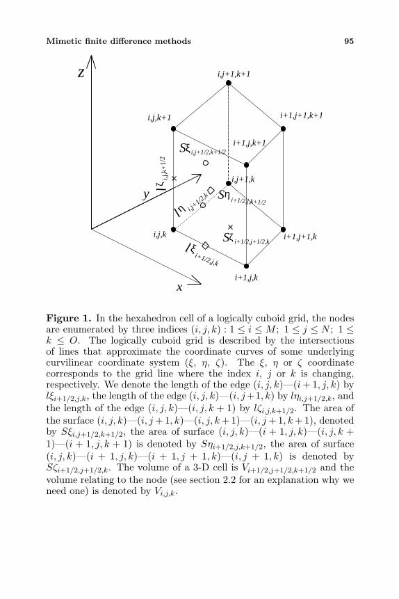
Mimetic finite difference methods 95
x
y
i,j,k
i+1,j,k
i+1,j+1,k
i,j+1,k
z
i,j,k+1
i+1,j,k+1
i,j+1,k+1
i+1,j+1,k+1
ζ i+1/2,j+1/2,k
ξ i,j+1/2,k+1/2S
ηi+1/2,j,k+1/2
S
Sl ξ
i+1/2,j,k
lη i,j+1/2,k
lζi,j
,k+
1/2
Figure 1. In the hexahedron cell of a logically cuboid grid, the nodesare enumerated by three indices (i, j, k) : 1 ≤ i ≤M ; 1 ≤ j ≤ N ; 1 ≤k ≤ O. The logically cuboid grid is described by the intersectionsof lines that approximate the coordinate curves of some underlyingcurvilinear coordinate system (ξ, η, ζ). The ξ, η or ζ coordinatecorresponds to the grid line where the index i, j or k is changing,respectively. We denote the length of the edge (i, j, k)—(i + 1, j, k) bylξi+1/2,j,k, the length of the edge (i, j, k)—(i, j+1, k) by lηi,j+1/2,k, andthe length of the edge (i, j, k)—(i, j, k + 1) by lζi,j,k+1/2. The area ofthe surface (i, j, k)—(i, j +1, k)—(i, j, k +1)—(i, j +1, k +1), denotedby Sξi,j+1/2,k+1/2, the area of surface (i, j, k)—(i + 1, j, k)—(i, j, k +1)—(i + 1, j, k + 1) is denoted by Sηi+1/2,j,k+1/2, the area of surface(i, j, k)—(i + 1, j, k)—(i + 1, j + 1, k)—(i, j + 1, k) is denoted bySζi+1/2,j+1/2,k. The volume of a 3-D cell is Vi+1/2,j+1/2,k+1/2 and thevolume relating to the node (see section 2.2 for an explanation why weneed one) is denoted by Vi,j,k.
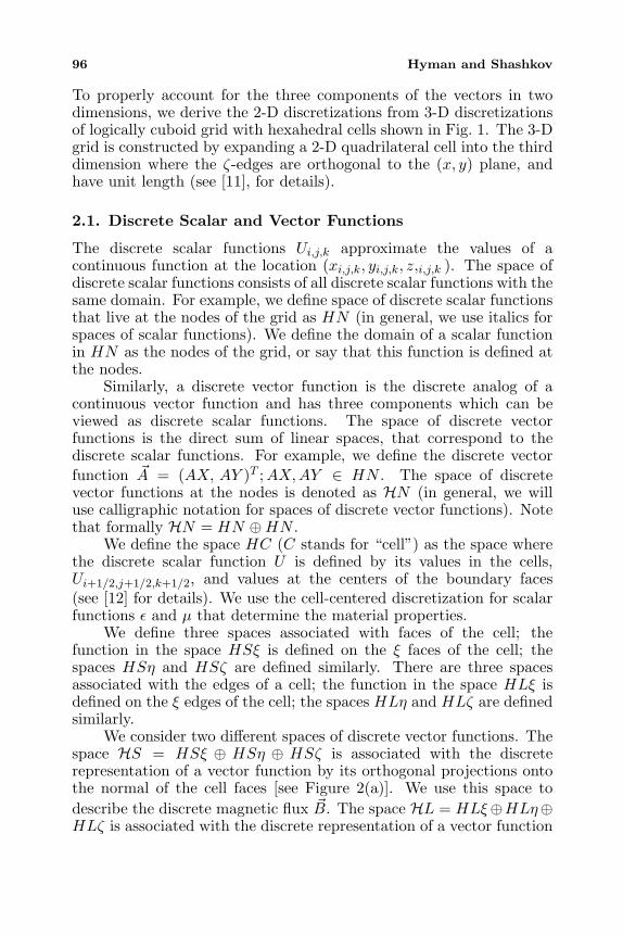
96 Hyman and Shashkov
To properly account for the three components of the vectors in twodimensions, we derive the 2-D discretizations from 3-D discretizationsof logically cuboid grid with hexahedral cells shown in Fig. 1. The 3-Dgrid is constructed by expanding a 2-D quadrilateral cell into the thirddimension where the ζ-edges are orthogonal to the (x, y) plane, andhave unit length (see [11], for details).
2.1. Discrete Scalar and Vector Functions
The discrete scalar functions Ui,j,k approximate the values of acontinuous function at the location (xi,j,k, yi,j,k, z,i,j,k ). The space ofdiscrete scalar functions consists of all discrete scalar functions with thesame domain. For example, we define space of discrete scalar functionsthat live at the nodes of the grid as HN (in general, we use italics forspaces of scalar functions). We define the domain of a scalar functionin HN as the nodes of the grid, or say that this function is defined atthe nodes.
Similarly, a discrete vector function is the discrete analog of acontinuous vector function and has three components which can beviewed as discrete scalar functions. The space of discrete vectorfunctions is the direct sum of linear spaces, that correspond to thediscrete scalar functions. For example, we define the discrete vectorfunction A = (AX, AY )T ;AX,AY ∈ HN . The space of discretevector functions at the nodes is denoted as HN (in general, we willuse calligraphic notation for spaces of discrete vector functions). Notethat formally HN = HN ⊕HN .
We define the space HC (C stands for “cell”) as the space wherethe discrete scalar function U is defined by its values in the cells,Ui+1/2,j+1/2,k+1/2, and values at the centers of the boundary faces(see [12] for details). We use the cell-centered discretization for scalarfunctions ε and µ that determine the material properties.
We define three spaces associated with faces of the cell; thefunction in the space HSξ is defined on the ξ faces of the cell; thespaces HSη and HSζ are defined similarly. There are three spacesassociated with the edges of a cell; the function in the space HLξ isdefined on the ξ edges of the cell; the spaces HLη and HLζ are definedsimilarly.
We consider two different spaces of discrete vector functions. Thespace HS = HSξ ⊕ HSη ⊕ HSζ is associated with the discreterepresentation of a vector function by its orthogonal projections ontothe normal of the cell faces [see Figure 2(a)]. We use this space todescribe the discrete magnetic flux B. The space HL = HLξ⊕HLη⊕HLζ is associated with the discrete representation of a vector function
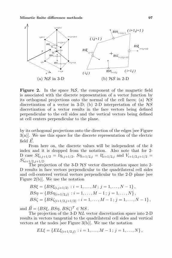
Mimetic finite difference methods 97
x
y
i,j,k
i+1,j,k
i+1,j+1,k
i,j+1,k
z
i,j,k+1
i+1,j,k+1
i,j+1,k+1
i+1,j+1,k+1
ξ
η
ζ
i,j+1/2,k+1/2
i+1/2,j,k+1/2
i+1/2,j+1/2,kBS
BS
BS
( i,j )( i+1,j )
( i+1,j+1 )
( i,j+1 )
ξ
ηS
SξS
ηS
Sζi+1/2,j+1/2
i,j+1/2
i+1/2,j
i+1,j+1/2
i+1/2,j+1
B
B
B
B
B
(a) HS in 3-D (b) HS in 2-D
Figure 2. In the space HS, the component of the magnetic fieldis associated with the discrete representation of a vector function byits orthogonal projections onto the normal of the cell faces; (a) HSdiscretization of a vector in 3-D; (b) 2-D interpretation of the HSdiscretization of a vector results in the face vectors being definedperpendicular to the cell sides and the vertical vectors being definedat cell centers perpendicular to the plane.
by its orthogonal projections onto the direction of the edges [see Figure3(a)]. We use this space for the discrete representation of the electricfield E.
From here on, the discrete values will be independent of the kindex and it is dropped from the notation. Also note that for 2-D case Sξi,j+1/2 = lηi,j+1/2, Sηi+1/2,j = lξi+1/2,j and Vi+1/2,j+1/2 =Sζi+1/2,j+1/2.
The projection of the 3-D HS vector discretization space into 2-D results in face vectors perpendicular to the quadrilateral cell sidesand cell-centered vertical vectors perpendicular to the 2-D plane [seeFigure 2(b)]. We use the notation
BSξ = BSξ(i,j+1/2) : i = 1, . . . ,M ; j = 1, . . . , N − 1 ,BSη = BSη(i+1/2,j) : i = 1, . . . ,M − 1 ; j = 1, . . . , N ,BSζ = BSζ(i+1/2,j+1/2) : i = 1, . . . ,M − 1 ; j = 1, . . . , N − 1 ,
and B = (BSξ, BSη, BSζ)T ∈ HS .The projection of the 3-D HL vector discretization space into 2-D
results in vectors tangential to the quadrilateral cell sides and verticalvectors at the nodes [see Figure 3(b)]. We use the notation
ELξ = ELξ(i+1/2,j) : i = 1, . . . ,M − 1 ; j = 1, . . . , N ,
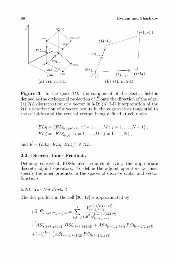
98 Hyman and Shashkov
x
y
i,j,k
i+1,j,k
i+1,j+1,k
i,j+1,k
z
i,j,k+1
i+1,j,k+1
i,j+1,k+1
i+1,j+1,k+1
ξ
η
ζ i,j,k+1/2
i+1/2,j,k
i,j+1/2,k
EL
EL
EL
( i,j )( i+1,j )
( i+1,j+1 )
( i,j+1 )
ξ
η
ζ i,jL
L
L
i+1/2,j
i,j+1/2
E
E
E
(a) HL in 3-D (b) HL in 2-D
Figure 3. In the space HL, the component of the electric field isdefined as the orthogonal projection of E onto the direction of the edge.(a) HL discretization of a vector in 3-D; (b) 2-D interpretation of theHL discretization of a vector results in the edge vectors tangential tothe cell sides and the vertical vectors being defined at cell nodes.
ELη = ELη(i,j+1/2) : i = 1, . . . ,M ; j = 1, . . . , N − 1 ,ELζ = ELζ(i,j) : i = 1, . . . ,M ; j = 1, . . . , N ,
and E = (ELξ, ELη, ELζ)T ∈ HL .
2.2. Discrete Inner Products
Defining consistent FDMs also requires deriving the appropriatediscrete adjoint operators. To define the adjoint operators we mustspecify the inner products in the spaces of discrete scalar and vectorfunctions.
2.2.1. The Dot Product
The dot product in the cell [30, 12] is approximated by
( A, B)(i+1/2,j+1/2) =1∑
k,l=0
V(i+1/2,j+1/2)(i+k,j+l)
sin2 ϕ(i+1/2,j+1/2)(i+k,j+l)
·[ASξ(i+k,j+1/2) BSξ(i+k,j+1/2) + ASη(i+1/2,j+l) BSη(i+1/2,j+l)
+(−1)k+l(ASξ(i+k,j+1/2) BSη(i+1/2,j+l)
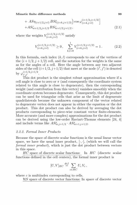
Mimetic finite difference methods 99
+ ASη(i+1/2,j+l) BSξ(i+k,j+1/2)
)cosϕ(i+1/2,j+1/2)
(i+k,j+l)
]+ASζi+1/2,j+1/2 BSζi+1/2,j+1/2 , (2.1)
where the weights V(i+1/2,j+1/2)(i+k,j+l) satisfy
V(i+1/2,j+1/2)(i+k,j+l) ≥ 0 ,
1∑k,l=0
V(i+1/2,j+1/2)(i+k,j+l) = 1 . (2.2)
In this formula, each index (k, l) corresponds to one of the vertices ofthe (i+ 1/2, j + 1/2) cell, and the notation for the weights is the sameas for the angles of a cell. Here the angle between any two adjacentsides of the cell (i+1/2, j+1/2) that meet at the node (i′, j′) is denotedby ϕ
i+1/2,j+1/2i′,j′ .This dot product is the simplest robust approximation where if a
cell angle is close to zero or π (and consequently the coordinate systemrelated to this angle is close to degenerate), then the correspondingweight (and contribution from this vertex) vanishes smoothly when thecoordinate system becomes degenerate. Consequently, this dot productcan be used for triangular cells that arise as the limit of degeneratequadrilaterals because the unknown component of the vector relatedto degenerate vertex does not appear in either the equation or the dotproduct. This dot product can also be derived by averaging the dotproducts corresponding to piece-wise constant vector finite-elements.More accurate (and more complex) approximations for the dot productcan be derived using the low-order Raviart-Thomas elements [24, 4]and include terms like ASξi,j+1/2 ·ASξi+1,j+1/2.
2.2.2. Formal Inner Products
Because the space of discrete scalar functions is the usual linear vectorspace, we have the usual inner product, [·, ·], (which we will call theformal inner product), which is just the dot product between vectorsin this space.
HC space of discrete scalar functions: In HC (discrete scalarfunctions defined in the cell centers), the formal inner product is
[U, V ]HCdef=
∑c∈HC
Uc Vc ,
where c is multiindex corresponding to cells.HS space of discrete vector functions: In space of discrete vector
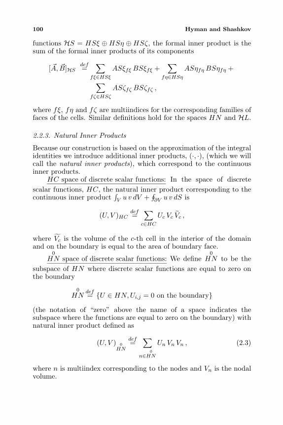
100 Hyman and Shashkov
functions HS = HSξ ⊕HSη ⊕HSζ, the formal inner product is thesum of the formal inner products of its components
[ A, B]HSdef=
∑fξ∈HSξ
ASξfξ BSξfξ +∑
fη∈HSηASηfη BSηfη +
∑fζ∈HSζ
ASζfζ BSζfζ ,
where fξ, fη and fζ are multiindices for the corresponding families offaces of the cells. Similar definitions hold for the spaces HN and HL.
2.2.3. Natural Inner Products
Because our construction is based on the approximation of the integralidentities we introduce additional inner products, (·, ·), (which we willcall the natural inner products), which correspond to the continuousinner products.
HC space of discrete scalar functions: In the space of discretescalar functions, HC, the natural inner product corresponding to thecontinuous inner product
∫V u v dV +
∮∂V u v dS is
(U, V )HCdef=
∑c∈HC
Uc Vc Vc ,
where Vc is the volume of the c-th cell in the interior of the domainand on the boundary is equal to the area of boundary face.
0HN space of discrete scalar functions: We define
0HN to be the
subspace of HN where discrete scalar functions are equal to zero onthe boundary
0HN
def= U ∈ HN,Ui,j = 0 on the boundary
(the notation of “zero” above the name of a space indicates thesubspace where the functions are equal to zero on the boundary) withnatural inner product defined as
(U, V ) 0HN
def=
∑n∈
0HN
Un Vn Vn , (2.3)
where n is multiindex corresponding to the nodes and Vn is the nodalvolume.
Mimetic finite difference methods 101
HS space of vector functions: In the space of vector functionsHS, the natural inner product corresponding to the continuous innerproduct
∫V ( A, B) dV is
( A, B)HSdef=
∑c∈HC
( A, B)c Vc , (2.4)
where ( A, B)c is the dot product of two discrete vectors defined by(2.1).
HL space of vector functions: The inner product inHL is similarto the inner product for space HS:
( A, B)HLdef=
∑c∈HC
( A, B)c Vc , (2.5)
where ( A, B)c approximates the dot product of two discrete vectorsfrom HL in the cell (see [12]), and looks similar to one for vectors fromHS.
2.2.4. Inner Product Identities
Natural discrete inner products satisfy the axioms of inner products,that is, they are true inner products and not just approximations of thecontinuous inner products. Also, discrete spaces are Euclidean spaces.
The natural and formal inner products satisfy the relationships
(U, V )HC = [C U, V ]HC , and ( A, B)HS = [S A, B]HS , (2.6)
where C : HC → HC and S : HS → HS are symmetric positiveoperators;
[C U, V ]HC = [U, C V ]HC , and [C U,U ]HC > 0 ,
[S A, B]HS = [ A,S B]HS , [S A, A]HS > 0 .
Therefore, the operator C satisfies the relations
(C U)c = Vc Uc , c ∈ HC .
The operator S can be written in block form,
S A =
S11 S12 0
S21 S22 00 0 S33
ASξ
ASηASζ
=
S11 ASξ + S12 ASη
S21 ASξ + S22 ASηS33 ASζ
.
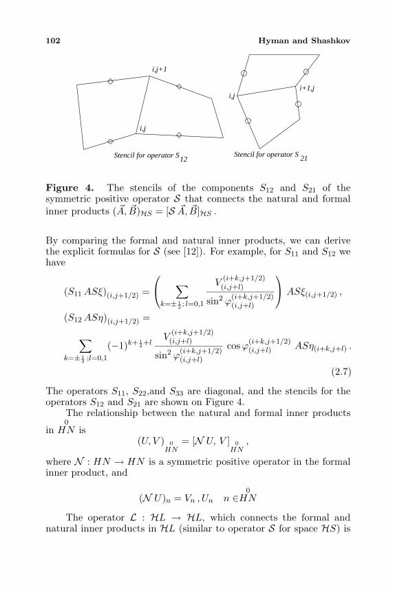
102 Hyman and Shashkov
i,j
i,j+1
Stencil for operator S12
i,ji+1,j
Stencil for operator S 21
Figure 4. The stencils of the components S12 and S21 of thesymmetric positive operator S that connects the natural and formalinner products ( A, B)HS = [S A, B]HS .
By comparing the formal and natural inner products, we can derivethe explicit formulas for S (see [12]). For example, for S11 and S12 wehave
(S11 ASξ)(i,j+1/2) =
∑k=± 1
2 ; l=0,1
V(i+k,j+1/2)(i,j+l)
sin2 ϕ(i+k,j+1/2)(i,j+l)
ASξ(i,j+1/2) ,
(S12 ASη)(i,j+1/2) =
∑k=± 1
2 ;l=0,1
(−1)k+ 12+l
V(i+k,j+1/2)(i,j+l)
sin2 ϕ(i+k,j+1/2)(i,j+l)
cosϕ(i+k,j+1/2)(i,j+l) ASη(i+k,j+l) .
(2.7)
The operators S11, S22,and S33 are diagonal, and the stencils for theoperators S12 and S21 are shown on Figure 4.
The relationship between the natural and formal inner products
in0
HN is(U, V ) 0
HN= [N U, V ] 0
HN,
where N : HN → HN is a symmetric positive operator in the formalinner product, and
(N U)n = Vn , Un n ∈0
HN
The operator L : HL → HL, which connects the formal andnatural inner products in HL (similar to operator S for space HS) is
Mimetic finite difference methods 103
symmetric and positive and can be written in block form as
L A =
L11 L12 0
L21 L22 00 0 L33
ALξ
ALηALζ
=
L11 ALξ + L12 ALη
L21 ALξ + L22 ALηL33 ALζ
.
The operators L11, L22, and L33 are diagonal, and the stencilsfor the operators L21 and L12 are the same as for the operators S12
and S21 (see Figure 4). Explicit expressions for these operators arepresented at [12].
3. DISCRETIZATION OF THE CURL OPERATORS
3.1. Discretization of curl E
We now describe how to construct a discrete curl that preserves adiscrete analog of Faraday’s law of electromagnetic induction locallyfor each face. The discrete analog of curl E in (1.1) acts on the discreteelectric field in HL as defined in Fig. 3 to create a vector in the samespace as the normal components of B on the cell faces to describe themagnetic flux (space HS in Fig. 2):
CURL : HL→ HS,
For this situation it is natural to use the coordinate invariant definitionof the curl E operator based on Stokes’ circulation theorem,
(n, curl E) = limS→0
∮L( E,l) dl
S. (3.8)
Here S is the surface spanning (based on) the closed curve L, n is theunit outward normal to S, and l is the unit tangential vector to L.In the discrete case the faces of the grid cells will be the surfaces Sin equation (3.8) and the “curve” L will be formed by edges of thecorresponding face.
Using the discrete analog of equation (3.8), we obtain expressionsfor components of vector R = (RSξ,RSη,RSζ)T = CURL E , where
RSξi,j+1/2 =ELζi,j+1 − ELζi,j
lηi,j+1/2,
RSηi+1/2,j = −ELζi+1,j − ELζi,jlξi+1/2,j
,
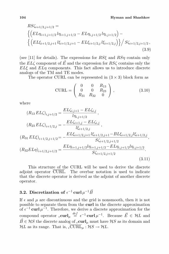
104 Hyman and Shashkov
RSζi+1/2,j+1/2 =(ELηi+1,j+1/2 lηi+1,j+1/2 − ELηi,j+1/2 lηi,j+1/2
)−(
ELξi+1/2,j+1 lξi+1/2,j+1 − ELξi+1/2,j lξi+1/2,j
)/Sζi+1/2,j+1/2 ,
(3.9)
(see [11] for details). The expressions for RSξ and RSη contain onlythe ELζ component of E and the expression for RSζ contains only theELξ and ELη components. This fact allows us to introduce discreteanalogs of the TM and TE modes.
The operator CURL can be represented in (3× 3) block form as
CURL =
0 0 R13
0 0 R23
R31 R32 0
, (3.10)
where
(R13 ELζ)i,j+1/2 =ELζi,j+1 − ELζi,j
lηi,j+1/2,
(R23 ELζ)i+1/2,j = −ELζi+1,j − ELζi,jlξi+1/2,j
,
(R31 ELξ)i+1/2,j+1/2= −ELξi+1/2,j+1 lξi+1/2,j+1−BLξi+1/2,jlξi+1/2,j
Sζi+1/2,j+1/2,
(R32ELη)i+1/2,j+1/2 =ELηi+1,j+1/2lηi+1,j+1/2−ELηi,j+1/2lηi,j+1/2
Sζi+1/2,j+1/2.
(3.11)
This structure of the CURL will be used to derive the discreteadjoint operator CURL. The overbar notation is used to indicatethat the discrete operator is derived as the adjoint of another discreteoperator.
3.2. Discretization of ε−1 curlµ−1 B
If ε and µ are discontinuous and the grid is nonsmooth, then it is notpossible to separate them from the curl in the discrete approximationof ε−1 curlµ−1. Therefore, we derive a discrete approximation for thecompound operator εcurlµ
def= ε−1 curlµ−1. Because E ∈ HL and
B ∈ HS the discrete analog of εcurlµ must have HS as its domain andHL as its range. That is, εCURLµ : HS → HL.
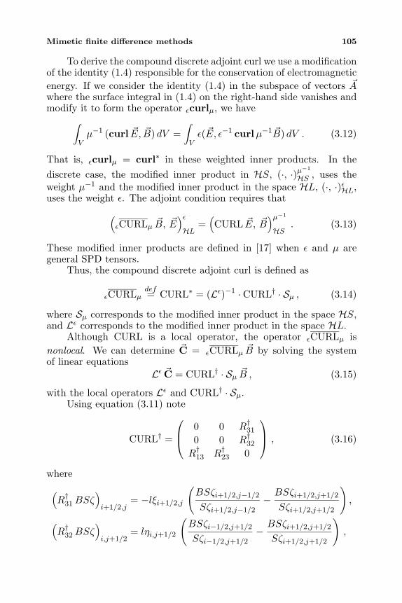
Mimetic finite difference methods 105
To derive the compound discrete adjoint curl we use a modificationof the identity (1.4) responsible for the conservation of electromagneticenergy. If we consider the identity (1.4) in the subspace of vectors Awhere the surface integral in (1.4) on the right-hand side vanishes andmodify it to form the operator εcurlµ, we have
∫Vµ−1 (curl E, B) dV =
∫Vε( E, ε−1 curlµ−1 B) dV . (3.12)
That is, εcurlµ = curl∗ in these weighted inner products. In thediscrete case, the modified inner product in HS, (·, ·)µ−1
HS , uses theweight µ−1 and the modified inner product in the space HL, (·, ·)εHL,uses the weight ε. The adjoint condition requires that
(εCURLµ B, E
)εHL
=(CURL E, B
)µ−1
HS. (3.13)
These modified inner products are defined in [17] when ε and µ aregeneral SPD tensors.
Thus, the compound discrete adjoint curl is defined as
εCURLµdef= CURL∗ = (Lε)−1 · CURL† · Sµ , (3.14)
where Sµ corresponds to the modified inner product in the space HS,and Lε corresponds to the modified inner product in the space HL.
Although CURL is a local operator, the operator εCURLµ isnonlocal. We can determine C = εCURLµ B by solving the systemof linear equations
Lε C = CURL† · Sµ B , (3.15)
with the local operators Lε and CURL† · Sµ.Using equation (3.11) note
CURL† =
0 0 R†310 0 R†32
R†13 R†23 0
, (3.16)
where
(R†31 BSζ
)i+1/2,j
= −lξi+1/2,j
(BSζi+1/2,j−1/2
Sζi+1/2,j−1/2−
BSζi+1/2,j+1/2
Sζi+1/2,j+1/2
),
(R†32 BSζ
)i,j+1/2
= lηi,j+1/2
(BSζi−1/2,j+1/2
Sζi−1/2,j+1/2−
BSζi+1/2,j+1/2
Sζi+1/2,j+1/2
),
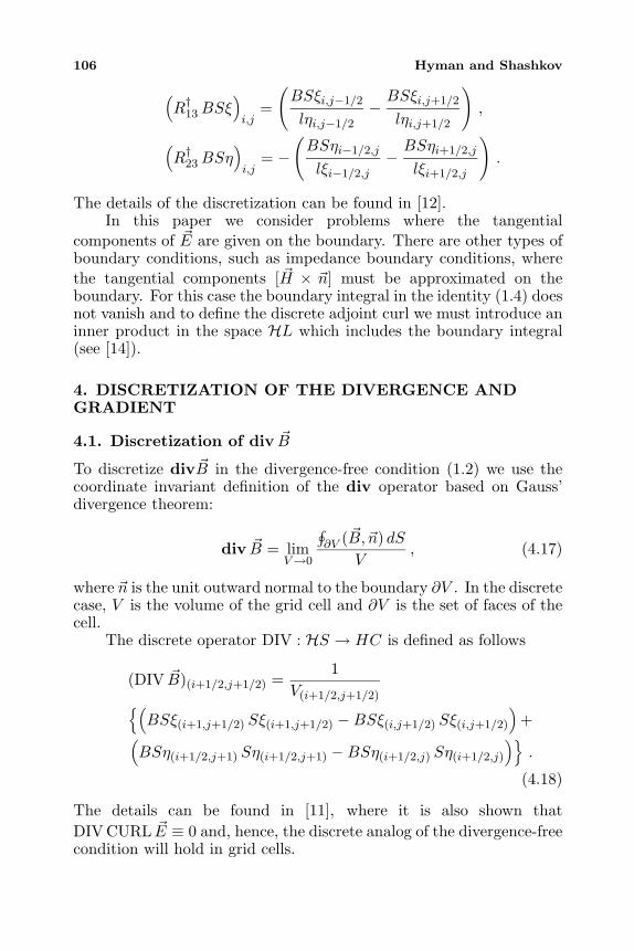
106 Hyman and Shashkov
(R†13 BSξ
)i,j
=
(BSξi,j−1/2
lηi,j−1/2−
BSξi,j+1/2
lηi,j+1/2
),
(R†23 BSη
)i,j
= −(BSηi−1/2,j
lξi−1/2,j−
BSηi+1/2,j
lξi+1/2,j
).
The details of the discretization can be found in [12].In this paper we consider problems where the tangential
components of E are given on the boundary. There are other types ofboundary conditions, such as impedance boundary conditions, wherethe tangential components [ H × n] must be approximated on theboundary. For this case the boundary integral in the identity (1.4) doesnot vanish and to define the discrete adjoint curl we must introduce aninner product in the space HL which includes the boundary integral(see [14]).
4. DISCRETIZATION OF THE DIVERGENCE ANDGRADIENT
4.1. Discretization of div B
To discretize div B in the divergence-free condition (1.2) we use thecoordinate invariant definition of the div operator based on Gauss’divergence theorem:
div B = limV→0
∮∂V ( B,n) dS
V, (4.17)
where n is the unit outward normal to the boundary ∂V . In the discretecase, V is the volume of the grid cell and ∂V is the set of faces of thecell.
The discrete operator DIV : HS → HC is defined as follows
(DIV B)(i+1/2,j+1/2) =1
V(i+1/2,j+1/2)(BSξ(i+1,j+1/2) Sξ(i+1,j+1/2) −BSξ(i,j+1/2) Sξ(i,j+1/2)
)+(
BSη(i+1/2,j+1) Sη(i+1/2,j+1) −BSη(i+1/2,j) Sη(i+1/2,j)
).
(4.18)
The details can be found in [11], where it is also shown thatDIV CURL E ≡ 0 and, hence, the discrete analog of the divergence-freecondition will hold in grid cells.
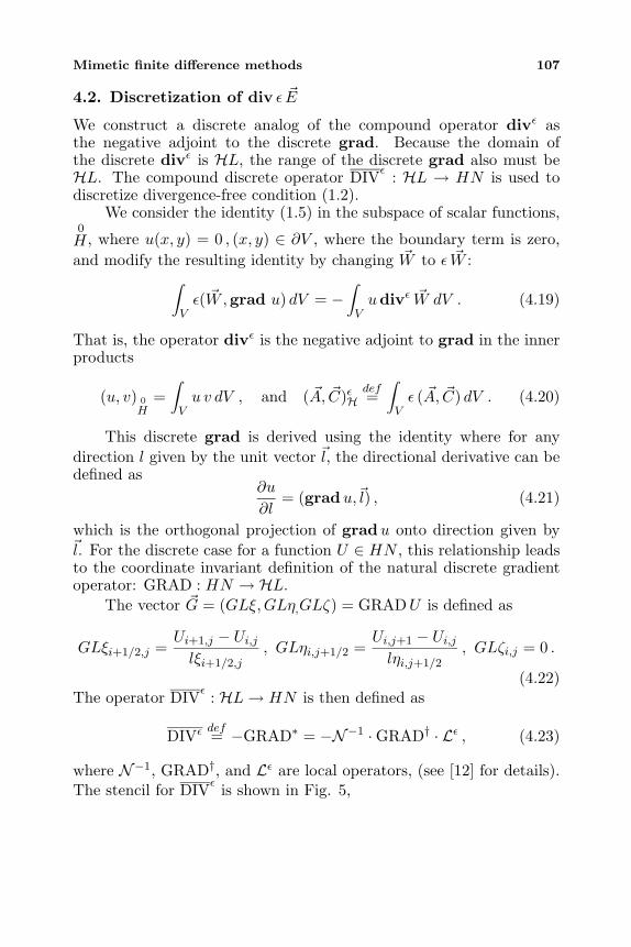
Mimetic finite difference methods 107
4.2. Discretization of div ε E
We construct a discrete analog of the compound operator divε asthe negative adjoint to the discrete grad. Because the domain ofthe discrete divε is HL, the range of the discrete grad also must beHL. The compound discrete operator DIVε : HL → HN is used todiscretize divergence-free condition (1.2).
We consider the identity (1.5) in the subspace of scalar functions,0H, where u(x, y) = 0 , (x, y) ∈ ∂V , where the boundary term is zero,and modify the resulting identity by changing W to ε W :
∫Vε( W,grad u) dV = −
∫Vudivε W dV . (4.19)
That is, the operator divε is the negative adjoint to grad in the innerproducts
(u, v) 0H
=∫Vu v dV , and ( A, C)εH
def=
∫Vε ( A, C) dV . (4.20)
This discrete grad is derived using the identity where for anydirection l given by the unit vector l, the directional derivative can bedefined as
∂u
∂l= (gradu,l) , (4.21)
which is the orthogonal projection of gradu onto direction given byl. For the discrete case for a function U ∈ HN , this relationship leadsto the coordinate invariant definition of the natural discrete gradientoperator: GRAD : HN → HL.
The vector G = (GLξ,GLη,GLζ) = GRADU is defined as
GLξi+1/2,j =Ui+1,j − Ui,j
lξi+1/2,j, GLηi,j+1/2 =
Ui,j+1 − Ui,jlηi,j+1/2
, GLζi,j = 0 .
(4.22)The operator DIVε : HL→ HN is then defined as
DIVεdef= −GRAD∗ = −N−1 ·GRAD† · Lε , (4.23)
where N−1, GRAD†, and Lε are local operators, (see [12] for details).The stencil for DIVε is shown in Fig. 5,
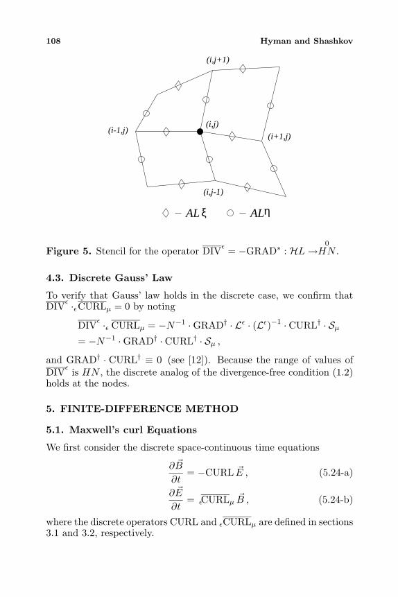
108 Hyman and Shashkov
(i,j)
(i+1,j)(i-1,j)
(i,j-1)
(i,j+1)
AL ALξ η
Figure 5. Stencil for the operator DIVε = −GRAD∗ : HL→0
HN .
4.3. Discrete Gauss’ Law
To verify that Gauss’ law holds in the discrete case, we confirm thatDIVε ·εCURLµ = 0 by noting
DIVε ·ε CURLµ = −N−1 ·GRAD† · Lε · (Lε)−1 · CURL† · Sµ= −N−1 ·GRAD† · CURL† · Sµ ,
and GRAD† · CURL† ≡ 0 (see [12]). Because the range of values ofDIVε is HN , the discrete analog of the divergence-free condition (1.2)holds at the nodes.
5. FINITE-DIFFERENCE METHOD
5.1. Maxwell’s curl Equations
We first consider the discrete space-continuous time equations
∂ B
∂t= −CURL E , (5.24-a)
∂ E
∂t= εCURLµ B , (5.24-b)
where the discrete operators CURL and εCURLµ are defined in sections3.1 and 3.2, respectively.
Mimetic finite difference methods 109
The conservation of electromagnetic energy for the discrete modelis the result of the consistent and compatible construction of thediscrete curl operators. The electric and magnetic part of the energycan be expressed in terms of the primary variables E and B as∫V
( D, E) dV =∫Vε ( E, E) dV ,
∫V
( B, H) dV =∫Vµ−1 ( B, B) dV .
The discrete analog of the electromagnetic energy is
EhEH =12
[( E, E)εHL + ( B, B)µ
−1
HL]. (5.25)
Taking the inner product (·, ·)µ−1
HS of B with both sides of equation(5.24-a) and similarly for (5.24-b) we obtain
(∂ B
∂t, B)µ
−1
HS = −(CURL E, B)µ−1
HS ,
(∂ E
∂t, E)εHL = (εCURLµ B, E)εHL .
By adding these two equations,
∂EhEH∂t
= −(CURL E, B)µ−1
HS + (εCURLµ B, E)εHL , (5.26)
and using (3.13), we note that the right side of this equation is zero.This corresponds to the preservation of energy when the tangentialcomponent of E is zero on the boundary. For the general case, incorrespondence with (1.4), the right side of the equation will be equalto a discrete approximation of corresponding the boundary integral.
The time discretization method
Bn+1 − Bn
∆t= −CURL Eα1 , (5.27-a)
En+1 − En
∆t= εCURLµ Bα2 , (5.27-b)
where Eα1 = α1En+1 + (1 − α1) En and Bα2 = α2
Bn+1 + (1 −α2) Bn, and tn = ∆t n, includes both explicit and implicit methods.respectively. For this integration method, if the discrete form of thedivergence free conditions (1.2)
DIVε En = 0 , (5.28-a)
DIV Bn = 0 , (5.28-b)
110 Hyman and Shashkov
(where DIVε and DIV are defined by equations (4.23) and (4.18)) aresatisfied initially, then they will be satisfied at later times [16].
Traditionally, because system (1.1) is hyperbolic, either the stableexplicit method (α1 = 0 or α2 = 0) or the explicit leapfrog method[19, 20] is used. For some problems, especially those with stronglydiscontinuous coefficients, it is important to preserve energy. The onlyscheme of form (5.27-a), (5.27-b) which preserves energy is the secondorder implicit midpoint method (α1 = α2 = 0.5) [16]. Also, thereare situations when the increased stability of an implicit method isnecessary to avoid taking extremely small time steps. This situationoccurs when computing the motion of fully electromagnetic particlesin the implosion of a laser fusion capsule [1]. Solution procedurefor system of linear equations corresponding to our discretization isdescribed in [16] (see also [30, 17, 23]).
The TM-mode equations for the BSξ, BSη components of themagnetic flux and the ELζ component of electric field are
BSξn+1 −BSξn
∆t= −R13 ELζα1 ,
BSηn+1 −BSηn
∆t= −R23 ELζα1 ,
Lε33ELζn+1 − ELζn
∆t=
(R †13 ·Sµ11 + R†23 · Sµ21
)BSξα2 +(
R †13 ·Sµ12 + R†23 · Sµ22
)BSηα2 .
The TE-mode equations for the BSζ component of the magneticflux and the ELξ, ELη components of the electric field are
BSζn+1 −BSζn
∆t= − (R31 ELξα1 + R32 ELηα1) ,
Lε11
ELξn+1 − ELξn
∆t+ Lε12
ELηn+1 − ELηn
∆t= R†31 Sµ33 BSζα2 ,
Lε21
ELξn+1 − ELξn
∆t+ Lε22
ELηn+1 − ELηn
∆t= R†32 Sµ33 BSζα2 .
5.2. Magnetic Diffusion Equations
The finite-difference equations for equations of magnetic field diffusionare
Bn+1 − Bn
∆t= −CURL Eα1 , (5.29-a)
En+1 = σCURLµ Bn+1 . (5.29-b)
Mimetic finite difference methods 111
The TM-mode equations are
BSξn+1 −BSξn
∆t= −R13 ELζα1 ,
BSηn+1 −BSηn
∆t= −R23 ELζα1 ,
Lσ33 ELζn+1 =(R †13 ·Sµ11 + R†23 · Sµ21
)BSξn+1 +(
R †13 ·Sµ12 + R†23 · Sµ22
)BSηn+1 .
The TE-mode equations are
BSζn+1 −BSζn
∆t= − (R31 ELξα1 + R32 ELηα1) ,
Lσ11 ELξn+1 + Lσ12 ELηn+1 = R†31 Sµ33 BSζn+1 ,
Lσ21 ELξn+1 + Lσ22 ELηn+1 = R†32 Sµ33 BSζn+1 . (5.30)
5.3. Rectangular Grids
On a rectangular (tensor product orthogonal) grid with constantspacing hx and hy, both operators Lε and Sµ are diagonal.
The TM-mode equations for the magnetic diffusion equations are
BSξn+1i,j+1/2 −BSξni,j+1/2
∆t= −
ELζα1i,j+1 − ELζα1
i,j
hy,
BSηn+1i+1/2,j −BSξni+1/2,j
∆t= +
ELζα1i+1,j − ELζα1
i,j
hx,
σi,jELζn+1i,j =
BSηn+1i+1/2,j
µi+1/2,j− BSηn+1
i−1/2,j
µi−1/2,j
hx−
BSξn+1i,j+1/2
µi,j+1/2− BSξn+1
i,j−1/2
µi,j−1/2
hy
where
σi,j =14
∑k=± 1
2,l=± 1
2
σi+k,j+l ,
µi,j+1/2 =12
(1
µi+1/2,j+1/2+
1µi−1/2,j+1/2
)−1
,
µi+1/2,j =12
(1
µi+1/2,j+1/2+
1µi+1/2,j−1/2
)−1
.
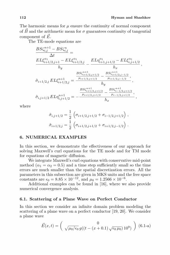
112 Hyman and Shashkov
The harmonic means for µ ensure the continuity of normal componentof B and the arithmetic mean for σ guarantees continuity of tangentialcomponent of E.
The TE-mode equations are
BSζn+1i,j −BSζni,j
∆t=
ELξα1
i+1/2,j+1 − ELξα1
i+1/2,j
hy−
ELηα1
i+1,j+1/2 − ELξα1
i,j+1/2
hx,
σi+1/2,j ELξn+1i+1/2,j =
BSζn+1i+1/2,j+1/2
µi+1/2,j+1/2− BSζn+1
i+1/2,j−1/2
µi+1/2,j−1/2,
hy,
σi,j+1/2 ELηn+1i,j+1/2 = −
BSζn+1i+1/2,j+1/2
µi+1/2,j+1/2− BSζn+1
i−1/2,j+1/2
µi−1/2,j+1/2,
hx,
where
σi,j+1/2 =12
(σi+1/2,j+1/2 + σi−1/2,j+1/2
),
σi+1/2,j =12
(σi+1/2,j+1/2 + σi+1/2,j−1/2
).
6. NUMERICAL EXAMPLES
In this section, we demonstrate the effectiveness of our approach forsolving Maxwell’s curl equations for the TE mode and for TM modefor equations of magnetic diffusion.
We integrate Maxwell’s curl equations with conservative mid-pointmethod (α1 = α2 = 0.5) and a time step sufficiently small so the timeerrors are much smaller than the spatial discretization errors. All theparameters in this subsection are given in MKS units and the free spaceconstants are ε0 = 8.85× 10⁻¹², and µ0 = 1.2566× 10⁻⁶.
Additional examples can be found in [16], where we also providenumerical convergence analysis.
6.1. Scattering of a Plane Wave on Perfect Conductor
In this section we consider an infinite domain problem modeling thescattering of a plane wave on a perfect conductor [19, 20]. We considera plane wave
E(x, t) =(
0√µ0/ε0 g((t− (x + 0.1)
√ε0 µ0) 109)
)(6.1-a)
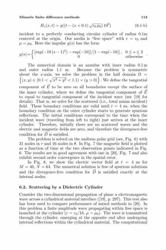
Mimetic finite difference methods 113
Hz(x, t) = g((t− (x + 0.1)√ε0 µ0) 109) (6.1-b)
incident to a perfectly conducting circular cylinder of radius 0.1mcentered at the origin. Our media is “free space” with ε = ε0 andµ = µ0. Here the impulse g(s) has the form
g(s)=
[exp(−10 (s− 1)2)− exp(−10)]/[1− exp(−10)] , 0 ≤ s ≤ 20 otherwise .
The numerical domain is an annulus with inner radius 0.1 mand outer radius 1.1 m. Because the problem is symmetricabout the x-axis, we solve the problem in the half domain Ω =(x, y) ∈ (0.1 <
√x2 + y2 < 1.1)× (y > 0)
. We define the tangential
component of E to be zero on all boundaries except the surface ofthe inner cylinder, where we define the tangential component of Eto equal to tangential component of the incident wave (see [19] fordetails). That is, we solve for the scattered (i.e., total minus incident)field. These boundary conditions are valid until t = 4 ns, when theboundary condition on the outer cylinder starts to generate spuriousreflections. The initial conditions correspond to the time when theincident wave (traveling from left to right) just arrives at the innercylinder. Therefore, initially there are no scattered waves and theelectric and magnetic fields are zero, and therefore the divergence-freecondition for D is satisfied.
The problem is solved on the uniform polar grid (see, Fig. 6) with31 nodes in r and 16 nodes in θ. In Fig. 7 the magnetic field is plottedas a function of time at the two observation points indicated in Fig.6. The results are in good agreement with one in [20], Fig. 7 and alsoexhibit second order convergence in the spatial error.
In Fig. 8, we show the electric vector field at t = 4 ns forM = 40, N = 64. The numerical solution is free of spurious solutionsand the divergence-free condition for D is satisfied exactly at theinternal nodes.
6.2. Scattering by a Dielectric Cylinder
Consider the two-dimensional propagation of plane a electromagneticwave across a cylindrical material interface ([19], p. 297). This test alsohas been used to compare performance of mixed methods in [20]. Inthis problem a finite amplitude wave propagating within free space islaunched at the cylinder (ε = ε0/16, µ = µ0). The wave is transmittedthrough the cylinder, emerging at the opposite end after undergoinginternal reflections within the cylindrical material. The computational
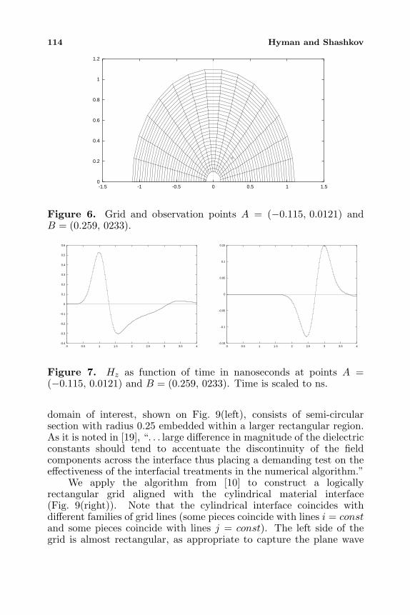
114 Hyman and Shashkov
0
0.2
0.4
0.6
0.8
1
1.2
-1.5 -1 -0.5 0 0.5 1 1.5
Figure 6. Grid and observation points A = (−0.115, 0.0121) andB = (0.259, 0233).
-0.4
-0.3
-0.2
-0.1
0
0.1
0.2
0.3
0.4
0.5
0.6
0 0.5 1 1.5 2 2.5 3 3.5 4-0.15
-0.1
-0.05
0
0.05
0.1
0.15
0 0.5 1 1.5 2 2.5 3 3.5 4
Figure 7. Hz as function of time in nanoseconds at points A =(−0.115, 0.0121) and B = (0.259, 0233). Time is scaled to ns.
domain of interest, shown on Fig. 9(left), consists of semi-circularsection with radius 0.25 embedded within a larger rectangular region.As it is noted in [19], “. . . large difference in magnitude of the dielectricconstants should tend to accentuate the discontinuity of the fieldcomponents across the interface thus placing a demanding test on theeffectiveness of the interfacial treatments in the numerical algorithm.”
We apply the algorithm from [10] to construct a logicallyrectangular grid aligned with the cylindrical material interface(Fig. 9(right)). Note that the cylindrical interface coincides withdifferent families of grid lines (some pieces coincide with lines i = constand some pieces coincide with lines j = const). The left side of thegrid is almost rectangular, as appropriate to capture the plane wave
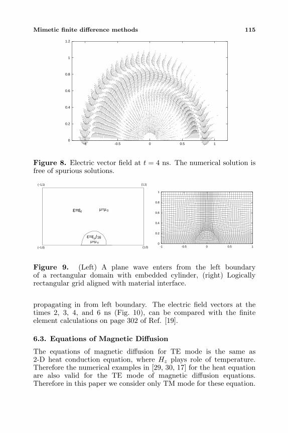
Mimetic finite difference methods 115
0
0.2
0.4
0.6
0.8
1
1.2
-1 -0.5 0 0.5 1
Figure 8. Electric vector field at t = 4 ns. The numerical solution isfree of spurious solutions.
ε=ε0 µ=µ 0
ε=ε /µ=µ 0
0 16
(−1,0) (1,0)
(−1,1) (1,1)
0
0.2
0.4
0.6
0.8
1
-1 -0.5 0 0.5 1
Figure 9. (Left) A plane wave enters from the left boundaryof a rectangular domain with embedded cylinder, (right) Logicallyrectangular grid aligned with material interface.
propagating in from left boundary. The electric field vectors at thetimes 2, 3, 4, and 6 ns (Fig. 10), can be compared with the finiteelement calculations on page 302 of Ref. [19].
6.3. Equations of Magnetic Diffusion
The equations of magnetic diffusion for TE mode is the same as2-D heat conduction equation, where Hz plays role of temperature.Therefore the numerical examples in [29, 30, 17] for the heat equationare also valid for the TE mode of magnetic diffusion equations.Therefore in this paper we consider only TM mode for these equation.
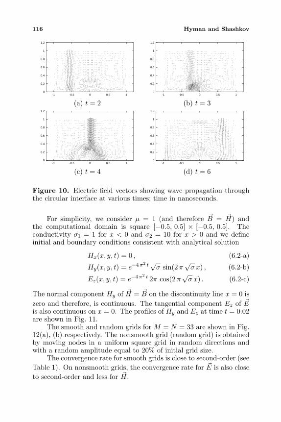
116 Hyman and Shashkov
0
0.2
0.4
0.6
0.8
1
1.2
-1 -0.5 0 0.5 10
0.2
0.4
0.6
0.8
1
1.2
-1 -0.5 0 0.5 1
(a) t = 2 (b) t = 3
0
0.2
0.4
0.6
0.8
1
1.2
-1 -0.5 0 0.5 10
0.2
0.4
0.6
0.8
1
1.2
-1 -0.5 0 0.5 1
(c) t = 4 (d) t = 6
Figure 10. Electric field vectors showing wave propagation throughthe circular interface at various times; time in nanoseconds.
For simplicity, we consider µ = 1 (and therefore B = H) andthe computational domain is square [−0.5, 0.5] × [−0.5, 0.5]. Theconductivity σ1 = 1 for x < 0 and σ2 = 10 for x > 0 and we defineinitial and boundary conditions consistent with analytical solution
Hx(x, y, t) = 0 , (6.2-a)
Hy(x, y, t) = e−4π2 t√σ sin(2π√σ x) , (6.2-b)
Ez(x, y, t) = e−4π2 t 2π cos(2π√σ x) . (6.2-c)
The normal component Hy of H = B on the discontinuity line x = 0 iszero and therefore, is continuous. The tangential component Ez of Eis also continuous on x = 0. The profiles of Hy and Ez at time t = 0.02are shown in Fig. 11.
The smooth and random grids for M = N = 33 are shown in Fig.12(a), (b) respectively. The nonsmooth grid (random grid) is obtainedby moving nodes in a uniform square grid in random directions andwith a random amplitude equal to 20% of initial grid size.
The convergence rate for smooth grids is close to second-order (seeTable 1). On nonsmooth grids, the convergence rate for E is also closeto second-order and less for H.
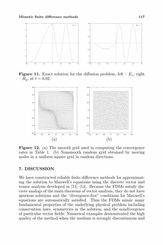
Mimetic finite difference methods 117
-3
-2
-1
0
1
2
3
-0.6 -0.4 -0.2 0 0.2 0.4 0.6
’Ez’
-1.5
-1
-0.5
0
0.5
1
1.5
-0.6 -0.4 -0.2 0 0.2 0.4 0.6
’Hy’
Figure 11. Exact solution for the diffusion problem, left – Ez, right– Hy, at t = 0.02.
-0.6
-0.4
-0.2
0
0.2
0.4
0.6
-0.6 -0.4 -0.2 0 0.2 0.4 0.6-0.6
-0.4
-0.2
0
0.2
0.4
0.6
-0.6 -0.4 -0.2 0 0.2 0.4 0.6
(a) (b)
Figure 12. (a) The smooth grid used in computing the convergencerates in Table 1. (b) Nonsmooth random grid obtained by movingnodes in a uniform square grid in random directions.
7. DISCUSSION
We have constructed reliable finite difference methods for approximat-ing the solution to Maxwell’s equations using the discrete vector andtensor analysis developed in [11]–[14]. Because the FDMs satisfy dis-crete analogs of the main theorems of vector analysis, they do not havespurious solutions and the “divergence-free” conditions for Maxwell’sequations are automatically satisfied. Thus the FDMs mimic manyfundamental properties of the underlying physical problem includingconservation laws, symmetries in the solution, and the nondivergenceof particular vector fields. Numerical examples demonstrated the highquality of the method when the medium is strongly discontinuous and
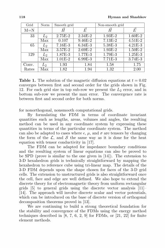
118 Hyman and Shashkov
Grid Norm Smooth grid Non-smooth grid
M=N H E H E
33 L2 2.75E-2 2.34E-2 1.93E-2 1.60E-2Max 0.107 9.46E-2 7.13E-2 4.51E-2
65 L2 7.16E-3 6.34E-3 5.38E-3 4.21E-3Max 3.57E-2 2.69E-2 1.93E-2 1.50E-2
129 L2 1.87E-3 1.77E-3 1.79E-3 1.25E-3Max 1.01E-2 6.99E-3 7.71E-3 3.74E-3
Conv. L2 1.93 1.84 1.58 1.75Rates Max 1.82 1.94 1.32 2.00
Table 1. The solution of the magnetic diffusion equations at t = 0.02converges between first and second order for the grids shown in Fig.12. For each grid size in top sub-row we present the L2 error, and inbottom sub-row we present the max error. The convergence rate isbetween first and second order for both norms.
for nonorthogonal, nonsmooth computational grids.By formulating the FDM in terms of coordinate invariant
quantities such as lengths, areas, volumes and angles, the resultingmethod can be used in any coordinate system by expressing thesequantities in terms of the particular coordinate system. The methodcan also be adapted to cases where ε, µ, and σ are tensors by changingthe form of the L, and S the same way as it is done for the heatequation with tensor conductivity in [17].
The FDM can be adapted for impedance boundary conditionsand the resulting system of linear equations can also be proved tobe SPD (prove is similar to the one given in [14]). The extension to3-D hexahedron grids is technically straightforward by mapping thehexahedron to reference cube using tri-linear map. The details of the3-D FDM depends upon the shape chosen for faces of the 3-D gridcells. The extension to unstructured grids is also straightforward oncethe cell, face and edge are well defined. We also hope to extend thediscrete theory for of electromagnetic theory from uniform rectangulargrids [5] to general grids using the discrete vector analysis [11]–[14]. The approach will involve discrete scalar and vector potentials,which can be introduced on the base of discrete version of orthogonaldecomposition theorems proved in [13].
We are continuing to build a strong theoretical foundation forthe stability and convergence of the FDMs using the energy methodtechniques described in [8, 7, 6, 2, 9] for FDMs, or [21, 22] for finiteelement methods.
Mimetic finite difference methods 119
ACKNOWLEGMENT
This work was performed under the auspices of the US Departmentof Energy (DOE) contract W-7405-ENG-36 and the DOE/MICSProgram in the Applied Mathematical Sciences contract KC-07-01-01. The authors would like to acknowledge D. Barnes, J. Morel,T. Oliphant Jr., S. Steinberg for many fruitful discussions, and R.Schuhmann for providing preprint of his recent work with T. Weiland,[27].
REFERENCES
1. Adam, A. C., A. G. Serveniere, J. C. Nedelec, and P. A. Raviart,“Study of an implicit scheme for integrating Maxwell’s equations,”Comput. Meth. Appl. Mech. Eng., Vol. 22, 327–346, 1980.
2. Ardelyan, N. V., “The Convergence of difference schemes fortwo-dimensional equations of acoustics and Maxwell’s equations,”USSR Comput. Math. and Math. Phys., Vol. 23, 93–99, 1983.
3. Bossavit, A., Computational Electromagnetism. VariationalFormulations, Complementarity, Edge Elements, Academic Press,1998.
4. Cai, Z., J. E. Jones, S. F. McCormick, and T. F. Russell, “Control-volume mixed finite element methods,” Comput. Geosci., Vol.1,289–315, 1997.
5. Chew, W. C., “Electromagnetic theory on a lattice,” J. Appl.Phys., Vol. 75, 4843–4850, 1994.
6. Denisov, A. A., A. V. Koldoba, and Yu. A. Poveshchenko,“The convergence to generalized solutions of difference schemesof the reference-operator method for Poisson’s equation,” USSRComput. Math. and Math. Phys., Vol. 29, 32–38, 1989.
7. Dmitrieva, M. V., A. A. Ivanov, V. F. Tishkin, and A. P. Favorskii,“Construction and investigation of support-operators finite-difference schemes for Maxwell equations in cylindrical geometry,”USSR Ac. of Sc., Vol. 27, Preprint Keldysh Inst. of Appl. Math.,1985 (in Russian).
8. Girault, V., “Theory of a finite difference methods on irregularnetworks,” SIAM J. Numer. Anal., Vol. 11, 260–282, 1974.
9. Gustafsson, B., H.-O. Kreiss, and J. Oliger, Time DependentProblems and Difference Methods, Vol. 11, 445–495, Wiley-Interscience Publication, John Wiley & Sons, Inc., 1995.
120 Hyman and Shashkov
10. Hyman, J. M., S. Li, P. Knupp, and M. Shashkov, “An algorithmto align a quadrilateral grid with internal boundaries,” J. Comp.Phys., Vol. 163, 133–149, 2000.
11. Hyman, J. M. and M. Shashkov, “Natural discretizations for thedivergence, gradient, and curl on logically rectangular grids,” Int.J. Computers & Math. with Applicat., Vol. 33,81–104, 1997.
12. Hyman, J. M. and M. Shashkov, “The adjoint operators for thenatural discretizations for the divergence, gradient, and curl onlogically rectangular grids,” IMACS J. Appl. Num. Math., Vol.25, 413–442, 1997.
13. Hyman, J. M. and M. Shashkov, “The orthogonal decompositiontheorems for mimetic finite difference methods,” SIAM J. Numer.Anal., Vol. 36, 788–818, 1999.
14. Hyman, J. M. and M. Shashkov, “The approximation ofboundary conditions for mimetic finite difference methods,” Int.J. Computers & Math. with Applicat., Vol. 36, 79–99, 1998.
15. Hyman, J. M. and M. Shashkov, “Mimetic discretizations forMaxwell’s equations and equations of magnetic diffusion,” ReportLA-UR-98-1032 (http://cnls.lanl.gov/∼shashkov) of Los AlamosNational Laboratory, Los Alamos, New Mexico, USA.
16. Hyman, J. M. and M. Shashkov, “Mimetic discretizations forMaxwell’s equations,” J. Comput. Phys., Vol. 151, 881–909, 1999.
17. Hyman, J. M., M. Shashkov, and S. Steinberg, “The numericalsolution of diffusion problems in strongly heterogeneous non-isotropic materials,” J. Comput. Phys., Vol. 132, 130–148, 1997.
18. Jin, J., The Finite Element Method in Electromagnetics, JohnWiley & Sons, Inc., New York, 1993.
19. Lee, R. L. and N. K. Madsen, “A mixed finite element formulationfor Maxwell’s equations in the time domain,” J. Comput. Phys.,Vol. 88, 284–304, 1990.
20. Monk, P., “A comparison of three mixed methods for the time-dependent Maxwell’s equations,” SIAM J. Sci. Stat. Comput.,Vol. 13, 1097–1122, 1992.
21. Monk, P., “Analysis of finite element method for Maxwell’sequations,” SIAM J. Num. Analysis, Vol. 29, 714–729, 1992.
22. Monk, P., “An analysis of Nedelec’s method for the spatialdiscretization of Maxwell’s equations,” J. Comp. Appl. Math., Vol.47, 101–121, 1993.
23. Morel, J. E., R. M. Roberts, and M. Shashkov, “A local support-operators diffusion discretization scheme for quadrilateral r-zmeshes,” J. Comput. Phys., Vol. 144, 17–51, 1998.
Mimetic finite difference methods 121
24. Raviart, P. A. and J. M. Thomas, “A mixed finite element methodfor 2-nd order elliptic Problems,” Mathematical Aspects of FiniteElement Methods, I. Galligani and E. Magenes (eds.), 292–315,Springer-Verlag, 1977.
25. Reitz, J. R., F. J. Milford, and R. W. Christy, Foundations ofElectromagnetic Theory, Third Edition, Chapters 16–18, 1980.
26. Samarskii, A. A., V. F. Tishkin, A. P. Favorskii, andM. Yu. Shashkov, “Operational finite-difference schemes,” Diff.Eqns., Vol. 17, 854–862, 1981.
27. Schuhmann, R. and T. Weiland, “Stability of the FDTD algorithmon nonorthogonal grids related to the spatial interpolationscheme,” IEEE Trans. Magn., Vol. 34, 2751–2754, 1998.
28. Shashkov, M., Conservative Finite-Difference Schemes on GeneralGrids, CRC Press, Boca Raton, Florida, 1995.
29. Shashkov, M. and S. Steinberg, “Support-operator finite-difference algorithms for general elliptic problems,” J. Comput.Phys., Vol. 118, 131–151, 1995.
30. Shashkov, M. and S. Steinberg, “Solving diffusion equations withrough coefficients in rough grids,” J. Comput. Phys., Vol. 129,383–405, 1996.
31. Finite Elements for Wave Electromagnetics. Methods andTechniques, P. P. Silvester and G. Pelosi (eds.), IEEE Press, NewYork, 1994.
32. Shercliff, J. A., A Textbook of Magnetohydrodynamics, 24,Pergamon Press, Oxford, 1965.
33. Teixeira, F. L. and W. C. Chew, “Lattice electromagnetic theoryfrom a topological viewpoint,” J. Math. Phys., Vol. 40, 169–187,1999.
34. Taflove, A., Computational Electrodynamics. The Finite-Difference Time-Domain Method, Artech House, Inc., Boston,1995.
35. Weiland, T., “Time domain electromagnetic field computationwith finite difference methods,” Int. J. Num. Model., Vol. 9, 295–319, 1996.
36. Yee, K. S., “Numerical solution of initial boundary value problemsinvolving Maxwell’s equations in isotropic media,” IEEE Trans.Antennas Propagat., Vol. 14, 302–307, 1966.
Progress In Electromagnetics Research, PIER 32, 123–149, 2001
THE GEOMETRY OF TIME-STEPPING
C. Mattiussi
Department of Micro-Engineering (DMT)Swiss Federal Institute of TechnologyCH-1015, Lausanne, Switzerland
Abstract—The space-time geometric structure of Maxwell’s equationsis examined and a subset of them is found to define a pair ofexact discrete time-stepping relations. The desirability of adoptingan approach to the discretization of electromagnetic problems whichexploits this fact is advocated, and the name topological time-steppingfor numerical schemes complying with it is suggested. The analysis ofthe equations leading to this kind of time-stepping reveals that theseequations are naturally written in terms of integrated field quantitiesassociated with space-time domains. It is therefore suggested thatthese quantities be adopted as state variables within numericalmethods. A list of supplementary prescriptions for a discretizationof electromagnetic problems suiting this philosophy is given, withparticular emphasis on the necessity to adopt a space-time approachin each discretization step. It is shown that some existing methodsalready comply with these tenets, but that this fact is not explicitlyrecognized and exploited. The role of the constitutive equations inthis discretization philosophy is briefly analyzed. The extension of thisapproach to more general kinds of space-time meshes, to other setsof basic time-stepping equations and to other field theories is finallyconsidered.
1 Introduction
2 The Founding Equations
3 The FDTD Time-Stepping Reconsidered
4 Topological Time-Stepping
5 The Missing Link
6 Generalizations
124 Mattiussi
7 Conclusions
References
1. INTRODUCTION
Time-domain methods for the full-wave analysis of three-dimensionalelectromagnetic problems, which include methods such as the Finite-Difference Time-Domain method (FDTD) and the Finite IntegrationTheory (FIT) method, are enjoying great popularity within theComputational Electromagnetics community. This is witnessed notonly by the amount of literature devoted to these methods but alsoby the appearance of several professional simulation packages whosecalculation engines are based on them, in addition to the moreestablished ones based on methods such as the Finite Element methodand the Method of Moments. A variety of reasons contribute tothe diffusion of time-domain methods, for example the possibility toobtain broadband data from a single simulation run, the favorable rateof growth of the required computational resources with the problemsize and complexity (provided a minimal critical mass of resources isavailable), and the existence of convincing implementations for manykinds of material models and boundary conditions. These favorableproperties seem able to balance the fact that the struggle to overcomethe limitations of the geometrical modeling capabilities traditionallyassociated with these methods does not appear to have fully succeededyet.
The present paper focuses on one aspect of time-domain methods,namely, time-stepping formulas, and shows that, with respect tothe traditional time-domain approaches, a fundamental improvementderived for time-domain methods from the adoption of a new time-stepping philosophy, which appears to be intrinsically built intothe physical laws of electromagnetism. This is made apparentby examining the geometrical backcloth on which these laws arefounded, an analysis which reveals the fundamental role played in thisimprovement by the adoption of a space-time approach (as opposed toone which discretizes separately the space and time variables).
A note of warning is in order about the approach and theterminology adopted within the present work. The concepts that aregoing to be presented can be given an elegant formulation using thelanguage of algebraic topology. However, since the adoption of thislanguage tends to obscure the simplicity and direct physical meaningof the concepts, that option is not pursued here. The interested readercan find in [5] a reformulation of most of the concepts treated in this
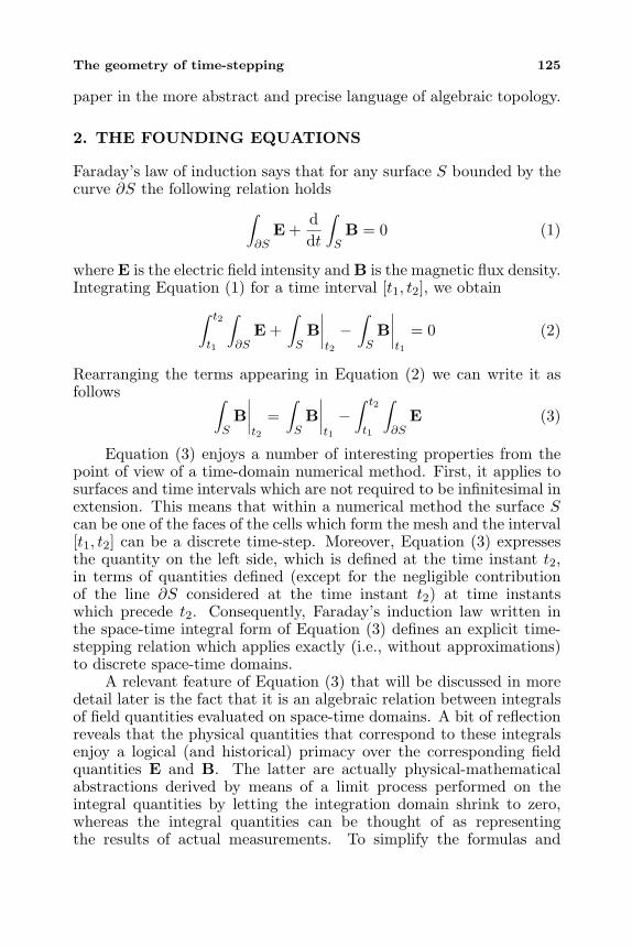
The geometry of time-stepping 125
paper in the more abstract and precise language of algebraic topology.
2. THE FOUNDING EQUATIONS
Faraday’s law of induction says that for any surface S bounded by thecurve ∂S the following relation holds
∫∂S
E +ddt
∫SB = 0 (1)
where E is the electric field intensity and B is the magnetic flux density.Integrating Equation (1) for a time interval [t1, t2], we obtain
∫ t2
t1
∫∂S
E +∫SB
∣∣∣∣t2
−∫SB
∣∣∣∣t1
= 0 (2)
Rearranging the terms appearing in Equation (2) we can write it asfollows ∫
SB
∣∣∣∣t2
=∫SB
∣∣∣∣t1
−∫ t2
t1
∫∂S
E (3)
Equation (3) enjoys a number of interesting properties from thepoint of view of a time-domain numerical method. First, it applies tosurfaces and time intervals which are not required to be infinitesimal inextension. This means that within a numerical method the surface Scan be one of the faces of the cells which form the mesh and the interval[t1, t2] can be a discrete time-step. Moreover, Equation (3) expressesthe quantity on the left side, which is defined at the time instant t2,in terms of quantities defined (except for the negligible contributionof the line ∂S considered at the time instant t2) at time instantswhich precede t2. Consequently, Faraday’s induction law written inthe space-time integral form of Equation (3) defines an explicit time-stepping relation which applies exactly (i.e., without approximations)to discrete space-time domains.
A relevant feature of Equation (3) that will be discussed in moredetail later is the fact that it is an algebraic relation between integralsof field quantities evaluated on space-time domains. A bit of reflectionreveals that the physical quantities that correspond to these integralsenjoy a logical (and historical) primacy over the corresponding fieldquantities E and B. The latter are actually physical-mathematicalabstractions derived by means of a limit process performed on theintegral quantities by letting the integration domain shrink to zero,whereas the integral quantities can be thought of as representingthe results of actual measurements. To simplify the formulas and
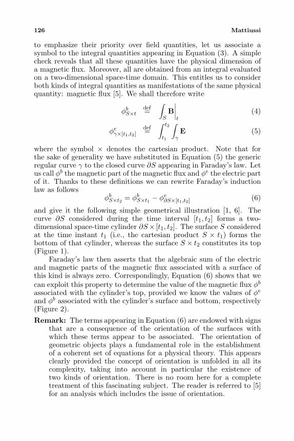
126 Mattiussi
to emphasize their priority over field quantities, let us associate asymbol to the integral quantities appearing in Equation (3). A simplecheck reveals that all these quantities have the physical dimension ofa magnetic flux. Moreover, all are obtained from an integral evaluatedon a two-dimensional space-time domain. This entitles us to considerboth kinds of integral quantities as manifestations of the same physicalquantity: magnetic flux [5]. We shall therefore write
φbS×tdef=
∫SB
∣∣∣∣t
(4)
φeγ×[t1,t2]def=
∫ t2
t1
∫γE (5)
where the symbol × denotes the cartesian product. Note that forthe sake of generality we have substituted in Equation (5) the genericregular curve γ to the closed curve ∂S appearing in Faraday’s law. Letus call φb the magnetic part of the magnetic flux and φe the electric partof it. Thanks to these definitions we can rewrite Faraday’s inductionlaw as follows
φbS×t2 = φbS×t1 − φe∂S×[t1,t2] (6)
and give it the following simple geometrical illustration [1, 6]. Thecurve ∂S considered during the time interval [t1, t2] forms a two-dimensional space-time cylinder ∂S× [t1, t2]. The surface S consideredat the time instant t1 (i.e., the cartesian product S × t1) forms thebottom of that cylinder, whereas the surface S × t2 constitutes its top(Figure 1).
Faraday’s law then asserts that the algebraic sum of the electricand magnetic parts of the magnetic flux associated with a surface ofthis kind is always zero. Correspondingly, Equation (6) shows that wecan exploit this property to determine the value of the magnetic flux φbassociated with the cylinder’s top, provided we know the values of φeand φb associated with the cylinder’s surface and bottom, respectively(Figure 2).
Remark: The terms appearing in Equation (6) are endowed with signsthat are a consequence of the orientation of the surfaces withwhich these terms appear to be associated. The orientation ofgeometric objects plays a fundamental role in the establishmentof a coherent set of equations for a physical theory. This appearsclearly provided the concept of orientation is unfolded in all itscomplexity, taking into account in particular the existence oftwo kinds of orientation. There is no room here for a completetreatment of this fascinating subject. The reader is referred to [5]for an analysis which includes the issue of orientation.
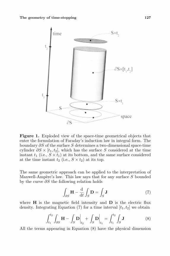
The geometry of time-stepping 127
Figure 1. Exploded view of the space-time geometrical objects thatenter the formulation of Faraday’s induction law in integral form. Theboundary ∂S of the surface S determines a two-dimensional space-timecylinder ∂S × [t1, t2], which has the surface S considered at the timeinstant t1 (i.e., S × t1) at its bottom, and the same surface consideredat the time instant t2 (i.e., S × t2) at its top.
The same geometric approach can be applied to the interpretation ofMaxwell-Ampere’s law. This law says that for any surface S boundedby the curve ∂S the following relation holds
∫∂S
H− ddt
∫SD =
∫SJ (7)
where H is the magnetic field intensity and D is the electric fluxdensity. Integrating Equation (7) for a time interval [t1, t2] we obtain
∫ t2
t1
∫∂S
H−∫SD
∣∣∣∣t2
+∫SD
∣∣∣∣t1
=∫ t2
t1
∫SJ (8)
All the terms appearing in Equation (8) have the physical dimension
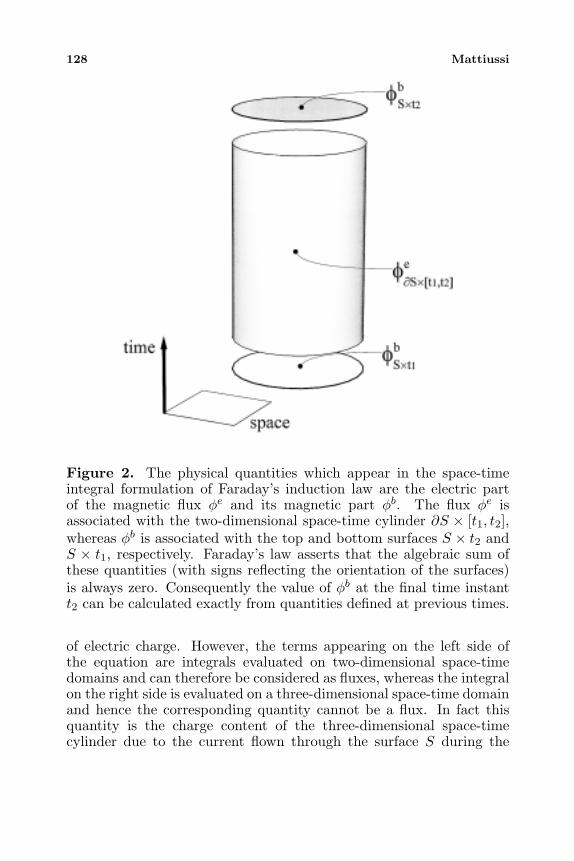
128 Mattiussi
Figure 2. The physical quantities which appear in the space-timeintegral formulation of Faraday’s induction law are the electric partof the magnetic flux φe and its magnetic part φb. The flux φe isassociated with the two-dimensional space-time cylinder ∂S × [t1, t2],whereas φb is associated with the top and bottom surfaces S × t2 andS × t1, respectively. Faraday’s law asserts that the algebraic sum ofthese quantities (with signs reflecting the orientation of the surfaces)is always zero. Consequently the value of φb at the final time instantt2 can be calculated exactly from quantities defined at previous times.
of electric charge. However, the terms appearing on the left side ofthe equation are integrals evaluated on two-dimensional space-timedomains and can therefore be considered as fluxes, whereas the integralon the right side is evaluated on a three-dimensional space-time domainand hence the corresponding quantity cannot be a flux. In fact thisquantity is the charge content of the three-dimensional space-timecylinder due to the current flown through the surface S during the
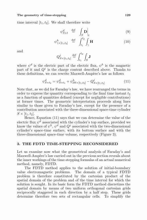
The geometry of time-stepping 129
time interval [t1, t2]. We shall therefore write
ψdS×tdef=
∫SD
∣∣∣∣t
(9)
ψhγ×[t1,t2]def=
∫ t2
t1
∫γH (10)
andQjS×[t1,t2]
def=∫ t2
t1
∫SJ
where ψd is the electric part of the electric flux, ψh is the magneticpart of it and Qj is the charge content described above. Thanks tothese definitions, we can rewrite Maxwell-Ampere’s law as follows
ψdS×t2 = ψdS×t1 + ψh∂S×[t1,t2] −QjS×[t1,t2] (11)
Note that, as we did for Faraday’s law, we have rearranged the terms inorder to express the quantity corresponding to the final time instant t2as a function of quantities defined (except for negligible contributions)at former times. The geometric interpretation proceeds along linessimilar to those given to Faraday’s law, except for the presence of acontribution associated with the three-dimensional space-time cylinderS × [t1, t2].
Hence, Equation (11) says that we can determine the value of theelectric flux ψd associated with the cylinder’s top surface, provided weknow the values of ψh, ψd and Qj associated with the two-dimensionalcylinder’s space-time surface, with its bottom surface and with thethree-dimensional space-time volume, respectively (Figure 3).
3. THE FDTD TIME-STEPPING RECONSIDERED
Let us examine now what the geometrical analysis of Faraday’s andMaxwell-Ampere’s law carried out in the previous section reveals aboutthe inner workings of the time-stepping formulas of an actual numericalmethod, namely, FDTD.
The FDTD method applies to the solution of initial-boundaryvalue electromagnetic problems. The domain of a typical FDTDproblem is therefore constituted by the cartesian product of thespatial domain of the problem and of the time interval for which thesolution is sought. In its basic form the FDTD method discretizes thespatial domain by means of two uniform orthogonal cartesian gridsreciprocally staggered in each direction by a half step. These gridsdetermine therefore two sets of rectangular cells. To simplify the
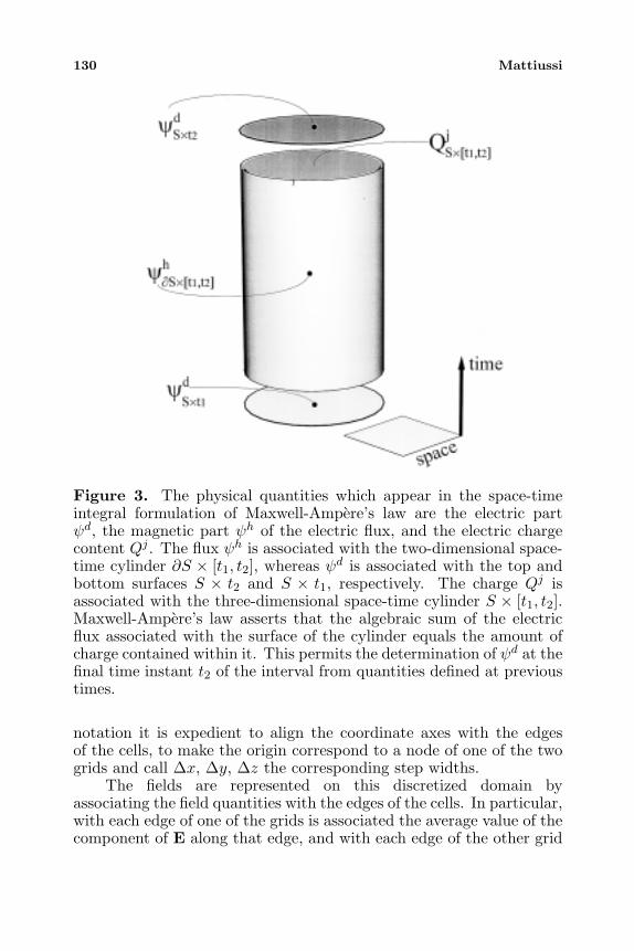
130 Mattiussi
Figure 3. The physical quantities which appear in the space-timeintegral formulation of Maxwell-Ampere’s law are the electric partψd, the magnetic part ψh of the electric flux, and the electric chargecontent Qj . The flux ψh is associated with the two-dimensional space-time cylinder ∂S × [t1, t2], whereas ψd is associated with the top andbottom surfaces S × t2 and S × t1, respectively. The charge Qj isassociated with the three-dimensional space-time cylinder S × [t1, t2].Maxwell-Ampere’s law asserts that the algebraic sum of the electricflux associated with the surface of the cylinder equals the amount ofcharge contained within it. This permits the determination of ψd at thefinal time instant t2 of the interval from quantities defined at previoustimes.
notation it is expedient to align the coordinate axes with the edgesof the cells, to make the origin correspond to a node of one of the twogrids and call ∆x, ∆y, ∆z the corresponding step widths.
The fields are represented on this discretized domain byassociating the field quantities with the edges of the cells. In particular,with each edge of one of the grids is associated the average value of thecomponent of E along that edge, and with each edge of the other grid
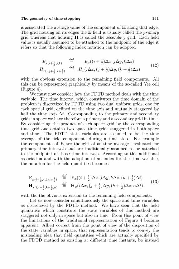
The geometry of time-stepping 131
is associated the average value of the component of H along that edge.The grid housing on its edges the E field is usually called the primarygrid whereas that housing H is called the secondary grid. Each fieldvalue is usually assumed to be attached to the midpoint of the edge itrefers so that the following index notation can be adopted
Ex(i+ 12,j,k)
def= Ex((i+ 12)∆x, j∆y, k∆z)
Hx(i,j+ 12,k+ 1
2)
def= Hx(i∆x, (j + 12)∆y, (k + 1
2)∆z)(12)
with the obvious extension to the remaining field components. Allthis can be represented graphically by means of the so-called Yee cell(Figure 4).
We must now consider how the FDTD method deals with the timevariable. The time interval which constitutes the time domain of theproblem is discretized by FDTD using two dual uniform grids, one foreach spatial grid, defined on the time axis and mutually staggered byhalf the time step ∆t. Corresponding to the primary and secondarygrids in space we have therefore a primary and a secondary grid in time.By considering the product of each space grid by the correspondingtime grid one obtains two space-time grids staggered in both spaceand time. The FDTD state variables are assumed to be the timeaverage of the field components during a time step. For examplethe components of E are thought of as time averages evaluated forprimary time intervals and are traditionally assumed to be attachedto the midpoint of those time intervals. According to this additionalassociation and with the adoption of an index for the time variable,the notation for the field quantities becomes
Ex(i+ 12,j,k,n+ 1
2)
def= Ex((i+ 12)∆x, j∆y, k∆z, (n+ 1
2)∆t)
Hx(i,j+ 12,k+ 1
2,n)
def= Hx(i∆x, (j + 12)∆y, (k + 1
2)∆z, n∆t)(13)
with the the obvious extension to the remaining field components.Let us now consider simultaneously the space and time variables
as discretized by the FDTD method. We have seen that the fieldquantities which constitute the state variables of this method arestaggered not only in space but also in time. From this point of viewthe limitations of the traditional representation of Figure 4 becomeapparent. Albeit correct from the point of view of the disposition ofthe state variables in space, that representation tends to convey themisleading idea that field quantities which are actually specified bythe FDTD method as existing at different time instants, be instead
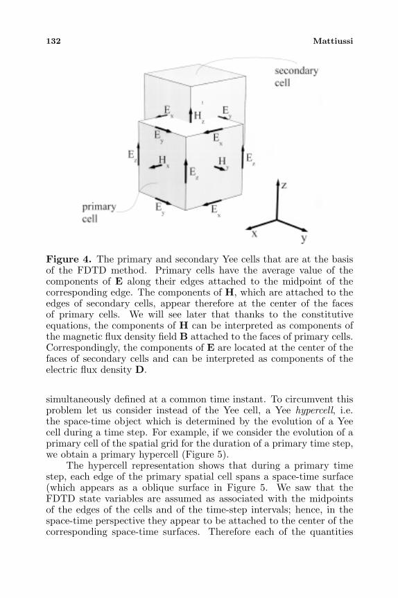
132 Mattiussi
Figure 4. The primary and secondary Yee cells that are at the basisof the FDTD method. Primary cells have the average value of thecomponents of E along their edges attached to the midpoint of thecorresponding edge. The components of H, which are attached to theedges of secondary cells, appear therefore at the center of the facesof primary cells. We will see later that thanks to the constitutiveequations, the components of H can be interpreted as components ofthe magnetic flux density field B attached to the faces of primary cells.Correspondingly, the components of E are located at the center of thefaces of secondary cells and can be interpreted as components of theelectric flux density D.
simultaneously defined at a common time instant. To circumvent thisproblem let us consider instead of the Yee cell, a Yee hypercell, i.e.the space-time object which is determined by the evolution of a Yeecell during a time step. For example, if we consider the evolution of aprimary cell of the spatial grid for the duration of a primary time step,we obtain a primary hypercell (Figure 5).
The hypercell representation shows that during a primary timestep, each edge of the primary spatial cell spans a space-time surface(which appears as a oblique surface in Figure 5. We saw that theFDTD state variables are assumed as associated with the midpointsof the edges of the cells and of the time-step intervals; hence, in thespace-time perspective they appear to be attached to the center of thecorresponding space-time surfaces. Therefore each of the quantities
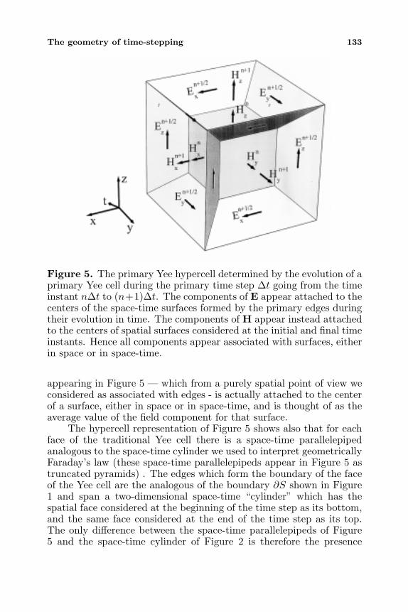
The geometry of time-stepping 133
Figure 5. The primary Yee hypercell determined by the evolution of aprimary Yee cell during the primary time step ∆t going from the timeinstant n∆t to (n+1)∆t. The components of E appear attached to thecenters of the space-time surfaces formed by the primary edges duringtheir evolution in time. The components of H appear instead attachedto the centers of spatial surfaces considered at the initial and final timeinstants. Hence all components appear associated with surfaces, eitherin space or in space-time.
appearing in Figure 5 — which from a purely spatial point of view weconsidered as associated with edges - is actually attached to the centerof a surface, either in space or in space-time, and is thought of as theaverage value of the field component for that surface.
The hypercell representation of Figure 5 shows also that for eachface of the traditional Yee cell there is a space-time parallelepipedanalogous to the space-time cylinder we used to interpret geometricallyFaraday’s law (these space-time parallelepipeds appear in Figure 5 astruncated pyramids) . The edges which form the boundary of the faceof the Yee cell are the analogous of the boundary ∂S shown in Figure1 and span a two-dimensional space-time “cylinder” which has thespatial face considered at the beginning of the time step as its bottom,and the same face considered at the end of the time step as its top.The only difference between the space-time parallelepipeds of Figure5 and the space-time cylinder of Figure 2 is therefore the presence
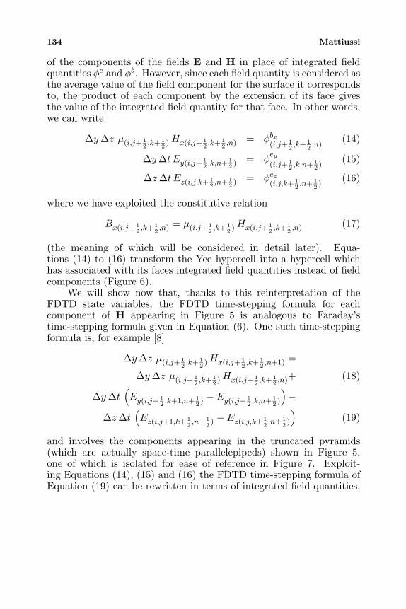
134 Mattiussi
of the components of the fields E and H in place of integrated fieldquantities φe and φb. However, since each field quantity is considered asthe average value of the field component for the surface it correspondsto, the product of each component by the extension of its face givesthe value of the integrated field quantity for that face. In other words,we can write
∆y∆z µ(i,j+ 12,k+ 1
2)Hx(i,j+ 1
2,k+ 1
2,n) = φbx
(i,j+ 12,k+ 1
2,n)
(14)
∆y∆t Ey(i,j+ 12,k,n+ 1
2) = φ
ey(i,j+ 1
2,k,n+ 1
2)
(15)
∆z∆t Ez(i,j,k+ 12,n+ 1
2) = φez
(i,j,k+ 12,n+ 1
2)
(16)
where we have exploited the constitutive relation
Bx(i,j+ 12,k+ 1
2,n) = µ(i,j+ 1
2,k+ 1
2)Hx(i,j+ 1
2,k+ 1
2,n) (17)
(the meaning of which will be considered in detail later). Equa-tions (14) to (16) transform the Yee hypercell into a hypercell whichhas associated with its faces integrated field quantities instead of fieldcomponents (Figure 6).
We will show now that, thanks to this reinterpretation of theFDTD state variables, the FDTD time-stepping formula for eachcomponent of H appearing in Figure 5 is analogous to Faraday’stime-stepping formula given in Equation (6). One such time-steppingformula is, for example [8]
∆y∆z µ(i,j+ 12,k+ 1
2)Hx(i,j+ 1
2,k+ 1
2,n+1) =
∆y∆z µ(i,j+ 12,k+ 1
2)Hx(i,j+ 1
2,k+ 1
2,n)+ (18)
∆y∆t(Ey(i,j+ 1
2,k+1,n+ 1
2) − Ey(i,j+ 1
2,k,n+ 1
2)
)−
∆z∆t(Ez(i,j+1,k+ 1
2,n+ 1
2) − Ez(i,j,k+ 1
2,n+ 1
2)
)(19)
and involves the components appearing in the truncated pyramids(which are actually space-time parallelepipeds) shown in Figure 5,one of which is isolated for ease of reference in Figure 7. Exploit-ing Equations (14), (15) and (16) the FDTD time-stepping formula ofEquation (19) can be rewritten in terms of integrated field quantities,
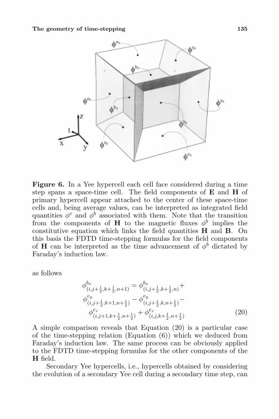
The geometry of time-stepping 135
Figure 6. In a Yee hypercell each cell face considered during a timestep spans a space-time cell. The field components of E and H ofprimary hypercell appear attached to the center of these space-timecells and, being average values, can be interpreted as integrated fieldquantities φe and φb associated with them. Note that the transitionfrom the components of H to the magnetic fluxes φb implies theconstitutive equation which links the field quantities H and B. Onthis basis the FDTD time-stepping formulas for the field componentsof H can be interpreted as the time advancement of φb dictated byFaraday’s induction law.
as follows
φbx(i,j+ 1
2,k+ 1
2,n+1)
= φbx(i,j+ 1
2,k+ 1
2,n)
+
φey(i,j+ 1
2,k+1,n+ 1
2)− φey
(i,j+ 12,k,n+ 1
2)−
φez(i,j+1,k+ 1
2,n+ 1
2)+ φez
(i,j,k+ 12,n+ 1
2)
(20)
A simple comparison reveals that Equation (20) is a particular caseof the time-stepping relation (Equation (6)) which we deduced fromFaraday’s induction law. The same process can be obviously appliedto the FDTD time-stepping formulas for the other components of theH field.
Secondary Yee hypercells, i.e., hypercells obtained by consideringthe evolution of a secondary Yee cell during a secondary time step, can
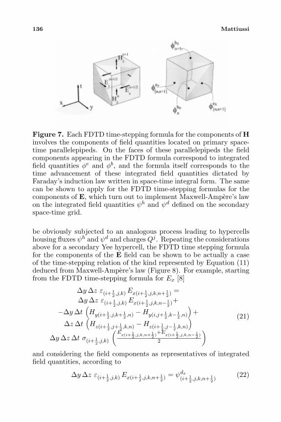
136 Mattiussi
Figure 7. Each FDTD time-stepping formula for the components of Hinvolves the components of field quantities located on primary space-time parallelepipeds. On the faces of these parallelepipeds the fieldcomponents appearing in the FDTD formula correspond to integratedfield quantities φe and φb, and the formula itself corresponds to thetime advancement of these integrated field quantities dictated byFaraday’s induction law written in space-time integral form. The samecan be shown to apply for the FDTD time-stepping formulas for thecomponents of E, which turn out to implement Maxwell-Ampere’s lawon the integrated field quantities ψh and ψd defined on the secondaryspace-time grid.
be obviously subjected to an analogous process leading to hypercellshousing fluxes ψh and ψd and chargesQj . Repeating the considerationsabove for a secondary Yee hypercell, the FDTD time stepping formulafor the components of the E field can be shown to be actually a caseof the time-stepping relation of the kind represented by Equation (11)deduced from Maxwell-Ampere’s law (Figure 8). For example, startingfrom the FDTD time-stepping formula for Ex [8]
∆y∆z ε(i+ 12,j,k)Ex(i+ 1
2,j,k,n+ 1
2) =
∆y∆z ε(i+ 12,j,k)Ex(i+ 1
2,j,k,n− 1
2)+
−∆y∆t(Hy(i+ 1
2,j,k+ 1
2,n) −Hy(i,j+ 1
2,k− 1
2,n)
)+
∆z∆t(Hz(i+ 1
2,j+ 1
2,k,n) −Hz(i+ 1
2,j− 1
2,k,n)
)
∆y∆z∆t σ(i+ 12,j,k)
(Ex(i+1
2 ,j,k,n+12 )
+Ex(i+1
2 ,j,k,n−12 )
2
)(21)
and considering the field components as representatives of integratedfield quantities, according to
∆y∆z ε(i+ 12,j,k)Ex(i+ 1
2,j,k,n+ 1
2) = ψdx
(i+ 12,j,k,n+ 1
2)
(22)
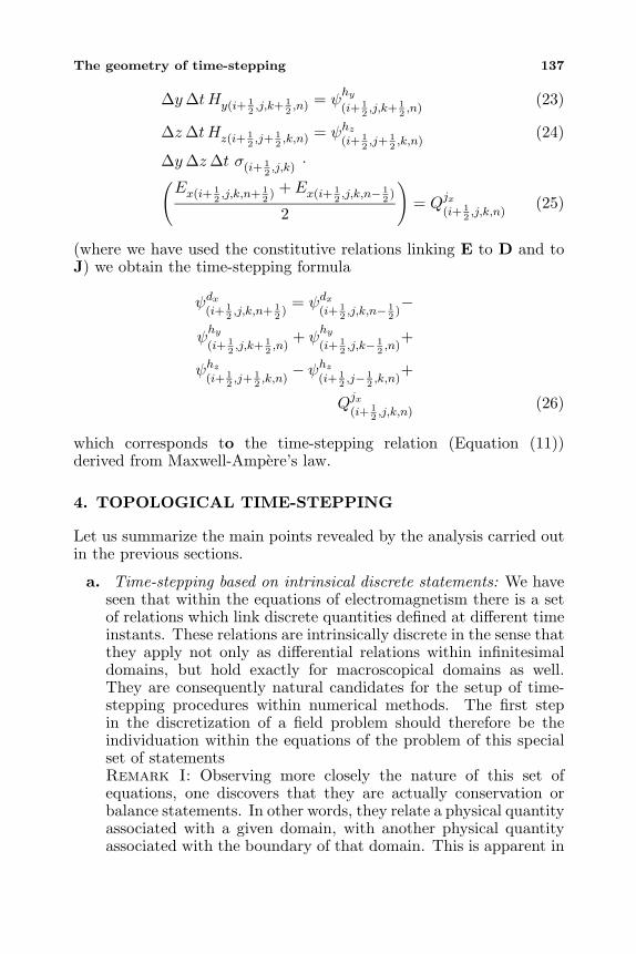
The geometry of time-stepping 137
∆y∆tHy(i+ 12,j,k+ 1
2,n) = ψ
hy(i+ 1
2,j,k+ 1
2,n)
(23)
∆z∆tHz(i+ 12,j+ 1
2,k,n) = ψhz
(i+ 12,j+ 1
2,k,n)
(24)
∆y∆z∆t σ(i+ 12,j,k) ·(
Ex(i+ 12,j,k,n+ 1
2) + Ex(i+ 1
2,j,k,n− 1
2)
2
)= Qjx
(i+ 12,j,k,n)
(25)
(where we have used the constitutive relations linking E to D and toJ) we obtain the time-stepping formula
ψdx(i+ 1
2,j,k,n+ 1
2)= ψdx
(i+ 12,j,k,n− 1
2)−
ψhy(i+ 1
2,j,k+ 1
2,n)
+ ψhy(i+ 1
2,j,k− 1
2,n)
+
ψhz(i+ 1
2,j+ 1
2,k,n)− ψhz
(i+ 12,j− 1
2,k,n)
+
Qjx(i+ 1
2,j,k,n)
(26)
which corresponds to the time-stepping relation (Equation (11))derived from Maxwell-Ampere’s law.
4. TOPOLOGICAL TIME-STEPPING
Let us summarize the main points revealed by the analysis carried outin the previous sections.
a. Time-stepping based on intrinsical discrete statements: We haveseen that within the equations of electromagnetism there is a setof relations which link discrete quantities defined at different timeinstants. These relations are intrinsically discrete in the sense thatthey apply not only as differential relations within infinitesimaldomains, but hold exactly for macroscopical domains as well.They are consequently natural candidates for the setup of time-stepping procedures within numerical methods. The first stepin the discretization of a field problem should therefore be theindividuation within the equations of the problem of this specialset of statementsRemark I: Observing more closely the nature of this set ofequations, one discovers that they are actually conservation orbalance statements. In other words, they relate a physical quantityassociated with a given domain, with another physical quantityassociated with the boundary of that domain. This is apparent in
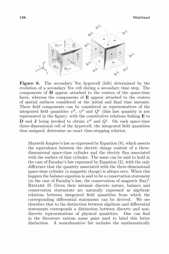
138 Mattiussi
Figure 8. The secondary Yee hypercell (left) determined by theevolution of a secondary Yee cell during a secondary time step. Thecomponents of H appear attached to the centers of the space-timefaces, whereas the components of E appear attached to the centersof spatial surfaces considered at the initial and final time instants.These field components can be considered as representatives of theintegrated field quantities ψh, ψd and Qj (this last quantity is notrepresented in the figure), with the constitutive relations linking E toD and J being invoked to obtain ψd and Qj . On each space-timethree-dimensional cell of the hypercell, the integrated field quantitiesthus assigned, determine an exact time-stepping relation.
Maxwell-Ampere’s law as expressed by Equation (8), which assertsthe equivalence between the electric charge content of a three-dimensional space-time cylinder and the electric flux associatedwith the surface of that cylinder. The same can be said to hold inthe case of Faraday’s law expressed by Equation (2), with the onlydifference that the quantity associated with the three-dimensionalspace-time cylinder (a magnetic charge) is always zero. When thishappen the balance equation is said to be a conservation statement(in the case of Faraday’s law, the conservation of magnetic flux)1Remark II: Given their intrinsic discrete nature, balance andconservation statements are naturally expressed as algebraicrelations between integrated field quantities from which thecorresponding differential statements can be derived. We seetherefore that to the distinction between algebraic and differentialstatements corresponds a distinction between discrete and non-discrete representations of physical quantities. One can findin the literature various name pairs used to label this latterdistinction. A nonexhaustive list includes the mathematically
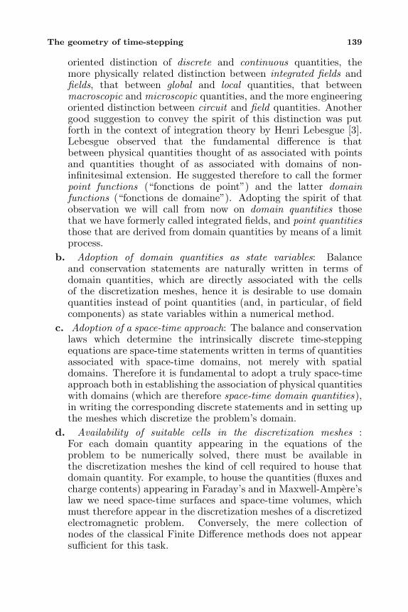
The geometry of time-stepping 139
oriented distinction of discrete and continuous quantities, themore physically related distinction between integrated fields andfields, that between global and local quantities, that betweenmacroscopic and microscopic quantities, and the more engineeringoriented distinction between circuit and field quantities. Anothergood suggestion to convey the spirit of this distinction was putforth in the context of integration theory by Henri Lebesgue [3].Lebesgue observed that the fundamental difference is thatbetween physical quantities thought of as associated with pointsand quantities thought of as associated with domains of non-infinitesimal extension. He suggested therefore to call the formerpoint functions (“fonctions de point”) and the latter domainfunctions (“fonctions de domaine”). Adopting the spirit of thatobservation we will call from now on domain quantities thosethat we have formerly called integrated fields, and point quantitiesthose that are derived from domain quantities by means of a limitprocess.
b. Adoption of domain quantities as state variables: Balanceand conservation statements are naturally written in terms ofdomain quantities, which are directly associated with the cellsof the discretization meshes, hence it is desirable to use domainquantities instead of point quantities (and, in particular, of fieldcomponents) as state variables within a numerical method.
c. Adoption of a space-time approach: The balance and conservationlaws which determine the intrinsically discrete time-steppingequations are space-time statements written in terms of quantitiesassociated with space-time domains, not merely with spatialdomains. Therefore it is fundamental to adopt a truly space-timeapproach both in establishing the association of physical quantitieswith domains (which are therefore space-time domain quantities),in writing the corresponding discrete statements and in setting upthe meshes which discretize the problem’s domain.
d. Availability of suitable cells in the discretization meshes :For each domain quantity appearing in the equations of theproblem to be numerically solved, there must be available inthe discretization meshes the kind of cell required to house thatdomain quantity. For example, to house the quantities (fluxes andcharge contents) appearing in Faraday’s and in Maxwell-Ampere’slaw we need space-time surfaces and space-time volumes, whichmust therefore appear in the discretization meshes of a discretizedelectromagnetic problem. Conversely, the mere collection ofnodes of the classical Finite Difference methods does not appearsufficient for this task.
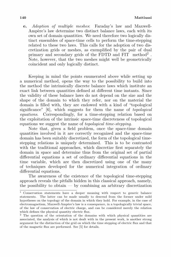
140 Mattiussi
e. Adoption of multiple meshes: Faraday’s law and Maxwell-Ampere’s law determine two distinct balance laws, each with itsown set of domain quantities. We need therefore two logically dis-tinct ensembles of space-time cells to perform the time-steppingrelated to these two laws. This calls for the adoption of two dis-cretization grids or meshes, as exemplified by the pair of dualprimary and secondary grids of the FDTD and FIT method2 .Note, however, that the two meshes might well be geometricallycoincident and only logically distinct.
Keeping in mind the points enumerated above while setting upa numerical method, opens the way to the possibility to build intothe method the intrinsically discrete balance laws which institute anexact link between quantities defined at different time instants. Sincethe validity of these balance laws do not depend on the size and theshape of the domain to which they refer, nor on the material thedomain is filled with, they are endowed with a kind of “topologicalsignificance” [6], which suggests for them the name of topologicalequations. Correspondingly, for a time-stepping relation based onthe exploitation of the intrinsic space-time discreteness of topologicalequations we suggest the name of topological time-stepping.
Note that, given a field problem, once the space-time domainquantities involved in it are correctly recognized and the space-timedomain has been suitably discretized, the form of the topological time-stepping relations is uniquely determined. This is to be contrastedwith the traditional approaches, which discretize first separately thedomain in space and determine thus from the original set of partialdifferential equations a set of ordinary differential equations in thetime variable, which are then discretized using one of the manyof techniques developed for the numerical integration of ordinarydifferential equations.
The awareness of the existence of the topological time-steppingapproach reveals the pitfalls hidden in this classical approach, namely,the possibility to obtain — by combining an arbitrary discretization1 Conservation statements have a deeper meaning with respect to generic balancestatements. The latter can be made usually to descend from the former under mildhypotheses on the topology of the domain in which they hold. For example, in the case ofelectromagnetism, Maxwell-Ampere’s law is a consequence, in a topologically trivial space,of the law of conservation of electric charge, and can be considered merely the relationwhich defines the physical quantity electric flux.2 The question of the orientation of the domains with which physical quantities areassociated, the analysis of which is not dealt with in the present work, is another strongargument for the distinction of the grid on which the time stepping of electric flux and thatof the magnetic flux are performed. See [5] for details.
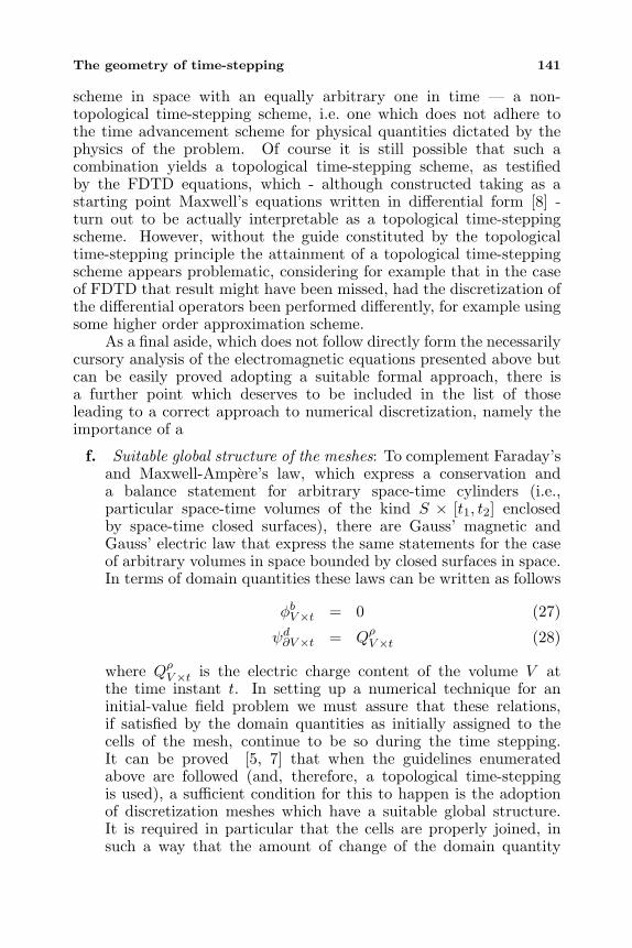
The geometry of time-stepping 141
scheme in space with an equally arbitrary one in time — a non-topological time-stepping scheme, i.e. one which does not adhere tothe time advancement scheme for physical quantities dictated by thephysics of the problem. Of course it is still possible that such acombination yields a topological time-stepping scheme, as testifiedby the FDTD equations, which - although constructed taking as astarting point Maxwell’s equations written in differential form [8] -turn out to be actually interpretable as a topological time-steppingscheme. However, without the guide constituted by the topologicaltime-stepping principle the attainment of a topological time-steppingscheme appears problematic, considering for example that in the caseof FDTD that result might have been missed, had the discretization ofthe differential operators been performed differently, for example usingsome higher order approximation scheme.
As a final aside, which does not follow directly form the necessarilycursory analysis of the electromagnetic equations presented above butcan be easily proved adopting a suitable formal approach, there isa further point which deserves to be included in the list of thoseleading to a correct approach to numerical discretization, namely theimportance of a
f. Suitable global structure of the meshes: To complement Faraday’sand Maxwell-Ampere’s law, which express a conservation anda balance statement for arbitrary space-time cylinders (i.e.,particular space-time volumes of the kind S × [t1, t2] enclosedby space-time closed surfaces), there are Gauss’ magnetic andGauss’ electric law that express the same statements for the caseof arbitrary volumes in space bounded by closed surfaces in space.In terms of domain quantities these laws can be written as follows
φbV×t = 0 (27)
ψd∂V×t = QρV×t (28)
where QρV×t is the electric charge content of the volume V atthe time instant t. In setting up a numerical technique for aninitial-value field problem we must assure that these relations,if satisfied by the domain quantities as initially assigned to thecells of the mesh, continue to be so during the time stepping.It can be proved [5, 7] that when the guidelines enumeratedabove are followed (and, therefore, a topological time-steppingis used), a sufficient condition for this to happen is the adoptionof discretization meshes which have a suitable global structure.It is required in particular that the cells are properly joined, insuch a way that the amount of change of the domain quantity
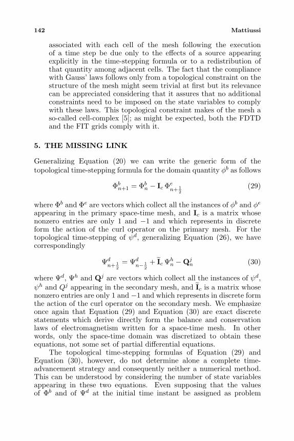
142 Mattiussi
associated with each cell of the mesh following the executionof a time step be due only to the effects of a source appearingexplicitly in the time-stepping formula or to a redistribution ofthat quantity among adjacent cells. The fact that the compliancewith Gauss’ laws follows only from a topological constraint on thestructure of the mesh might seem trivial at first but its relevancecan be appreciated considering that it assures that no additionalconstraints need to be imposed on the state variables to complywith these laws. This topological constraint makes of the mesh aso-called cell-complex [5]; as might be expected, both the FDTDand the FIT grids comply with it.
5. THE MISSING LINK
Generalizing Equation (20) we can write the generic form of thetopological time-stepping formula for the domain quantity φb as follows
Φbn+1 = Φb
n − Ic Φen+ 1
2(29)
where Φb and Φe are vectors which collect all the instances of φb and φeappearing in the primary space-time mesh, and Ic is a matrix whosenonzero entries are only 1 and −1 and which represents in discreteform the action of the curl operator on the primary mesh. For thetopological time-stepping of ψd, generalizing Equation (26), we havecorrespondingly
Ψdn+ 1
2= Ψd
n− 12
+ Ic Ψhn −Qj
n (30)
where Ψd, Ψh and Qj are vectors which collect all the instances of ψd,ψh and Qj appearing in the secondary mesh, and Ic is a matrix whosenonzero entries are only 1 and −1 and which represents in discrete formthe action of the curl operator on the secondary mesh. We emphasizeonce again that Equation (29) and Equation (30) are exact discretestatements which derive directly form the balance and conservationlaws of electromagnetism written for a space-time mesh. In otherwords, only the space-time domain was discretized to obtain theseequations, not some set of partial differential equations.
The topological time-stepping formulas of Equation (29) andEquation (30), however, do not determine alone a complete time-advancement strategy and consequently neither a numerical method.This can be understood by considering the number of state variablesappearing in these two equations. Even supposing that the valuesof Φb and of Ψd at the initial time instant be assigned as problem
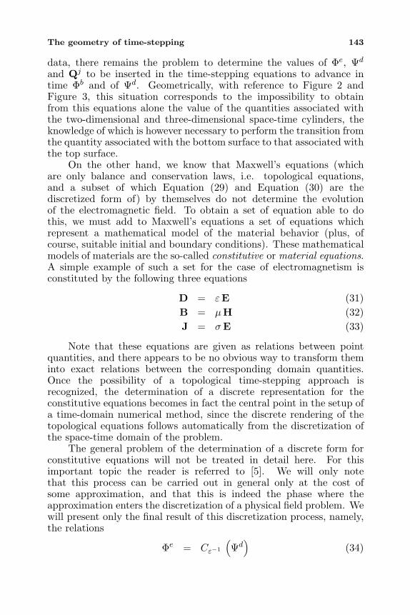
The geometry of time-stepping 143
data, there remains the problem to determine the values of Φe, Ψd
and Qj to be inserted in the time-stepping equations to advance intime Φb and of Ψd. Geometrically, with reference to Figure 2 andFigure 3, this situation corresponds to the impossibility to obtainfrom this equations alone the value of the quantities associated withthe two-dimensional and three-dimensional space-time cylinders, theknowledge of which is however necessary to perform the transition fromthe quantity associated with the bottom surface to that associated withthe top surface.
On the other hand, we know that Maxwell’s equations (whichare only balance and conservation laws, i.e. topological equations,and a subset of which Equation (29) and Equation (30) are thediscretized form of) by themselves do not determine the evolutionof the electromagnetic field. To obtain a set of equation able to dothis, we must add to Maxwell’s equations a set of equations whichrepresent a mathematical model of the material behavior (plus, ofcourse, suitable initial and boundary conditions). These mathematicalmodels of materials are the so-called constitutive or material equations.A simple example of such a set for the case of electromagnetism isconstituted by the following three equations
D = εE (31)B = µH (32)J = σE (33)
Note that these equations are given as relations between pointquantities, and there appears to be no obvious way to transform theminto exact relations between the corresponding domain quantities.Once the possibility of a topological time-stepping approach isrecognized, the determination of a discrete representation for theconstitutive equations becomes in fact the central point in the setup ofa time-domain numerical method, since the discrete rendering of thetopological equations follows automatically from the discretization ofthe space-time domain of the problem.
The general problem of the determination of a discrete form forconstitutive equations will not be treated in detail here. For thisimportant topic the reader is referred to [5]. We will only notethat this process can be carried out in general only at the cost ofsome approximation, and that this is indeed the phase where theapproximation enters the discretization of a physical field problem. Wewill present only the final result of this discretization process, namely,the relations
Φe = Cε−1
(Ψd
)(34)
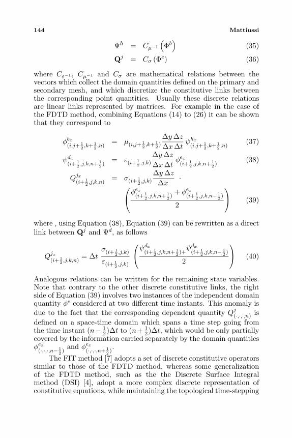
144 Mattiussi
Ψh = Cµ−1
(Φb
)(35)
Qj = Cσ (Φe) (36)
where Cε−1 , Cµ−1 and Cσ are mathematical relations between thevectors which collect the domain quantities defined on the primary andsecondary mesh, and which discretize the constitutive links betweenthe corresponding point quantities. Usually these discrete relationsare linear links represented by matrices. For example in the case ofthe FDTD method, combining Equations (14) to (26) it can be shownthat they correspond to
φbx(i,j+ 1
2,k+ 1
2,n)
= µ(i,j+ 12,k+ 1
2)
∆y∆z∆x∆t
ψhx(i,j+ 1
2,k+ 1
2,n)
(37)
ψdx(i+ 1
2,j,k,n+ 1
2)
= ε(i+ 12,j,k)
∆y∆z∆x∆t
φex(i+ 1
2,j,k,n+ 1
2)
(38)
Qjx(i+ 1
2,j,k,n)
= σ(i+ 12,j,k)
∆y∆z∆x
·φex
(i+ 12,j,k,n+ 1
2)+ φex
(i+ 12,j,k,n− 1
2)
2
(39)
where , using Equation (38), Equation (39) can be rewritten as a directlink between Qj and Ψd, as follows
Qjx(i+ 1
2,j,k,n)
= ∆tσ(i+ 1
2,j,k)
ε(i+ 12,j,k)
ψdx
(i+ 12,j,k,n+ 1
2)+ψdx
(i+ 12,j,k,n− 1
2)
2
(40)
Analogous relations can be written for the remaining state variables.Note that contrary to the other discrete constitutive links, the rightside of Equation (39) involves two instances of the independent domainquantity φe considered at two different time instants. This anomaly isdue to the fact that the corresponding dependent quantity Qj(·,·,·,n) isdefined on a space-time domain which spans a time step going fromthe time instant (n− 1
2)∆t to (n+ 12)∆t, which would be only partially
covered by the information carried separately by the domain quantitiesφex
(·,·,·,n− 12)
and φex(·,·,·,n+ 1
2).
The FIT method [7] adopts a set of discrete constitutive operatorssimilar to those of the FDTD method, whereas some generalizationof the FDTD method, such as the the Discrete Surface Integralmethod (DSI) [4], adopt a more complex discrete representation ofconstitutive equations, while maintaining the topological time-stepping
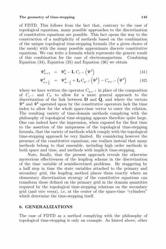
The geometry of time-stepping 145
of FDTD. This follows from the fact that, contrary to the case oftopological equations, many possible approaches to the discretizationof constitutive equations are possible. This fact opens the way to theconstruction of a multiplicity of methods based on the combinationof the unique topological time-stepping formula (for a given choice ofthe mesh) with the many possible approximate discrete constitutiveequations. We can write a formula which represents the generic resultof this combination for the case of electromagnetism. CombiningEquation (34), Equation (35) and Equation (36) we obtain
Φbn+1 = Φb
n − Ir Cε−1
(Ψd
)(41)
Ψdn+ 1
2= Ψd
n− 12
+ IdCµ−1
(Φb
)− Cσ,ε−1
(Ψd
)(42)
where we have written the operator Cσ,ε−1 in place of the compositionof Cε−1 and Cσ to allow for a more general approach to thediscretization of the link between D and Q, and where the vectorsΨd and Φb operated upon by the constitutive operators lack the timeindex to allow for the whole space-time vector to enter the relation.The resulting variety of time-domain methods complying with thephilosophy of topological time-stepping appears therefore quite large.One can indeed have the impression, when exposed for the first timeto the assertion of the uniqueness of the topological time-steppingformula, that the variety of methods which comply with the topologicaltime-stepping approach be very limited. By considering however thepresence of the constitutive equations, one realizes instead that manymethods belong to that ensemble, including high order methods inboth space and time, and methods with implicit time-stepping.
Note, finally, that the present approach reveals the otherwisemysterious effectiveness of the leapfrog scheme in the discretizationof the time variable of semidiscretized problems. By staggering bya half step in time the state variables attached to the primary andsecondary grid, the leapfrog method places them exactly where anelementary discretization strategy of the constitutive equations cantransform those defined on the primary grid in the domain quantitiesrequired by the topological time-stepping relations on the secondarygrid (and vice versa), i.e, at the center of the space-time “cylinders”which determine the time-stepping itself.
6. GENERALIZATIONS
The case of FDTD as a method complying with the philosophy oftopological time-stepping is only an example. As hinted above, other
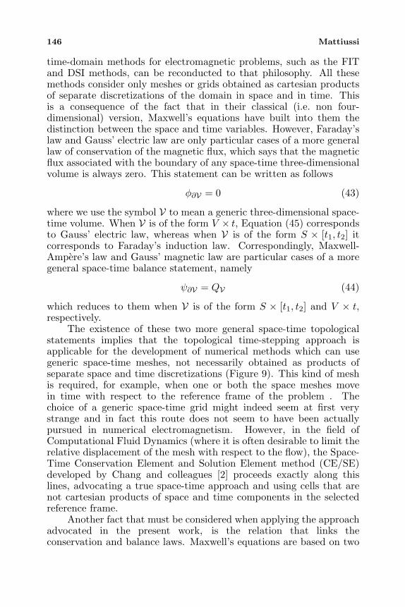
146 Mattiussi
time-domain methods for electromagnetic problems, such as the FITand DSI methods, can be reconducted to that philosophy. All thesemethods consider only meshes or grids obtained as cartesian productsof separate discretizations of the domain in space and in time. Thisis a consequence of the fact that in their classical (i.e. non four-dimensional) version, Maxwell’s equations have built into them thedistinction between the space and time variables. However, Faraday’slaw and Gauss’ electric law are only particular cases of a more generallaw of conservation of the magnetic flux, which says that the magneticflux associated with the boundary of any space-time three-dimensionalvolume is always zero. This statement can be written as follows
φ∂V = 0 (43)
where we use the symbol V to mean a generic three-dimensional space-time volume. When V is of the form V × t, Equation (45) correspondsto Gauss’ electric law, whereas when V is of the form S × [t1, t2] itcorresponds to Faraday’s induction law. Correspondingly, Maxwell-Ampere’s law and Gauss’ magnetic law are particular cases of a moregeneral space-time balance statement, namely
ψ∂V = QV (44)
which reduces to them when V is of the form S × [t1, t2] and V × t,respectively.
The existence of these two more general space-time topologicalstatements implies that the topological time-stepping approach isapplicable for the development of numerical methods which can usegeneric space-time meshes, not necessarily obtained as products ofseparate space and time discretizations (Figure 9). This kind of meshis required, for example, when one or both the space meshes movein time with respect to the reference frame of the problem . Thechoice of a generic space-time grid might indeed seem at first verystrange and in fact this route does not seem to have been actuallypursued in numerical electromagnetism. However, in the field ofComputational Fluid Dynamics (where it is often desirable to limit therelative displacement of the mesh with respect to the flow), the Space-Time Conservation Element and Solution Element method (CE/SE)developed by Chang and colleagues [2] proceeds exactly along thislines, advocating a true space-time approach and using cells that arenot cartesian products of space and time components in the selectedreference frame.
Another fact that must be considered when applying the approachadvocated in the present work, is the relation that links theconservation and balance laws. Maxwell’s equations are based on two
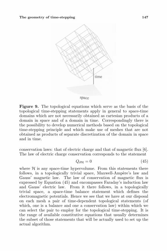
The geometry of time-stepping 147
Figure 9. The topological equations which serve as the basis of thetopological time-stepping statements apply in general to space-timedomains which are not necessarily obtained as cartesian products of adomain in space and of a domain in time. Correspondingly there isthe possibility to develop numerical methods based on the topologicaltime-stepping principle and which make use of meshes that are notobtained as products of separate discretization of the domain in spaceand in time.
conservation laws: that of electric charge and that of magnetic flux [6].The law of electric charge conservation corresponds to the statement
Q∂H = 0 (45)
where H is any space-time hypervolume. From this statements therefollows, in a topologically trivial space, Maxwell-Ampere’s law andGauss’ magnetic law. The law of conservation of magnetic flux isexpressed by Equation (45) and encompasses Faraday’s induction lawand Gauss’ electric law. From it there follows, in a topologicallytrivial space, a space-time balance statement which defines theelectromagnetic potentials. Hence we see that we have at our disposalon each mesh a pair of time-dependent topological statements (ofwhich, one is a balance and one a conservation law) within which wecan select the pair to employ for the topological time-stepping. It isthe range of available constitutive equations that usually determinesthe subset of those statements that will be actually used to set up theactual algorithm.
148 Mattiussi
Finally, it is worth noting that the example of the CE/SE methodmentioned above reveals that what said here about electromagnetismapplies also to other field theories. In fact it is clear that this approachapplies to all field theories which have within their equations a setof space-time topological statements, i.e. of space-time balance orconservation laws. Since this is true for almost all non-static physicalfield theories, the scope of the topological time-stepping philosophyappears indeed very broad.
7. CONCLUSIONS
We have shown that electromagnetism has built into its equationsa set of intrinsically discrete time-dependent statements which canserve as a natural basis of a numerical time-stepping strategy. Whenthe space-time domain of a problem has been discretized, thesestatements translate directly into a set of time-stepping relations,provided the proper space-time meshes have been defined and thecorresponding integrated field quantities have been selected as statevariables. Moreover, the role of constitutive equations in thediscretization process stands out very clearly once the intrinsicallydiscrete statements have been singled out. This approach calls forthe adoption of a space-time point of view in all phases of thediscretization process. An analysis of some successful time-domainmethods reveals however that until now the intrinsic space-timediscreteness the electromagnetic equations has not been explicitlyacknowledged and exploited by numerical methods (although in somecases, for example the FIT method, the intrinsic discreteness in spacehas been recognized). The correction of this state of affairs can bringadvantages both from the point of view of the comprehension and finetuning of existing methods and of the development of new ones. Thisapplies not only to electromagnetism but also to generic physical fieldtheories, and it appears desirable that in all these cases the approachpresented here be built into numerical methods from the start and thefavorable properties which ensue, at last fully enjoyed.
REFERENCES
1. Bamberg, P. and S. Sternberg, A Course in Mathematicsfor Students of Physics: 1–2, Cambridge University Press,Cambridge, 1988.
2. Chang, S. C., X. Y. Wang, and C. Y. Chow, “The space-timeconservation element and solution element method: A new high-
The geometry of time-stepping 149
resolution and genuinely multidimensional paradigm for solvingconservation laws,” J. Comput. Phys., Vol. 56, 89–136, 1999.
3. Lebesgue, H., Lecons sur l’Integration, Chelsea, New York, 1973.4. Madsen, N. K., “Divergence preserving discrete surface integral
methods for Maxwell’s curl equations using non-orthogonalunstructured grids,” J. Comput. Phys., Vol. 119, 34–45, 1995.
5. Mattiussi, C., “The finite volume, finite element, and finitedifference methods as numerical methods for physical fieldproblems,” Advances in Imaging and Electron Physics, P. Hawkes(ed.), Vol. 113, 1–146, 2000.
6. Truesdell, C. and R. A. Toupin, “The classical field theories,”Handbuch der Physik, S. Flugge (ed.), Vol. 3/1, 226–793, Springer-Verlag, Berlin, 1960.
7. Weiland, T., “Time domain electromagnetic field computationwith finite difference methods,” Int. J. Numer. Modelling, Vol. 9,295–319, 1996.
8. Yee, K. S., “Numerical solution of initial boundary value problemsinvolving Maxwell’s equations in isotropic media,” IEEE Trans.Antennas Propagat., Vol. 14, 302–307, 1966.
Progress In Electromagnetics Research, PIER 32, 151–169, 2001
DATA STRUCTURES FOR GEOMETRIC ANDTOPOLOGICAL ASPECTS OF FINITE ELEMENTALGORITHMS
P. W. Gross
Mathematical Sciences Research Institute1000 Centennial Drive, Berkeley, CA 94720, USA
P. R. Kotiuga
Department of Electrical and Computer EngineeringBoston University8 Saint Mary’s St., Boston, MA 02215, USA
Abstract—This paper uses simplicial complexes and simplicial(co)homology theory to expose a foundation for data structures fortetrahedral finite element meshes. Identifying tetrahedral mesheswith simplicial complexes leads, by means of Whitney forms, to theconnection between simplicial cochains and fields in the region modeledby the mesh. Furthermore, lumped field parameters are tied tomatrices associated with simplicial (co)homology groups. The datastructures described here are sparse, and the computational complexityof constructing them is O(n) where n is the number of vertices in thefinite element mesh. Non-tetrahedral meshes can be handled by anequivalent theory. These considerations lead to a discrete form ofPoincare duality which is a powerful tool for developing algorithmsfor topological computations on finite element meshes. This dualityemerges naturally in the data structures. We indicate some practicalapplications of both data structures and underlying theory.
1 Introduction1.1 Outline
2 The Complex Encoded in the Connection Matrix2.1 Background and Definitions2.2 From Connection Data to Chain Groups2.3 Considerations for Cellular Meshes
152 Gross and Kotiuga
3 The Cochain Complex3.1 Simplicial Cochain Groups and the Coboundary Operator3.2 Coboundary Data Structures
4 Application: Whitney Forms4.1 Example: The Helicity Functional
5 The Dual Complex and Discrete Poincare Duality for(Co)Chains
6 Applications6.1 Simplicial (Co)Homology6.2 Cuts for Magnetic Scalar Potentials
7 Conclusion
Acknowledgment
References
1. INTRODUCTION
In many algorithms for finite element applications there arecomputations which do not depend on the metric of the space. In thesecases, once the vertex coordinates are used to ascribe an orientation(±1) to the elements of the mesh, it is only the finite elementconnection matrix which is left to play a purely integer combinatorialrole in the computation which handles the topological business of thealgorithm. More precisely, the connection matrix alone contains awealth of topological information about the discretized region, realizingits simplicial or cellular complex [22].
The complex is an old and venerable idea in algebraic topologyand electrical circuit theory [19], but has not attracted much attentionin 3-dimensional finite elements technology. Moreover, it is intimatelyconnected to homology and cohomology theories which are an algebraicexpression of how the topology of a region is tied to fields in the regionand is the formalism which links fields in the continuum to lumpedcircuit parameters [13]. Nevertheless, the profound consequences ofthis algebraic structure can be seen in the computation of cuts formagnetic scalar potentials [11, 5], discretization of the magnetic helicityfunctional [6], and Whitney forms for finite elements [21, 9, 3]. Moregenerally, the same data structures are related to presentations of thefundamental group of the triangulated region, sparse matrix techniquesfor 3-d finite elements, and, when the metric of the space is introduced,general 3-d finite element computations.
Data structures for finite elements 153
In this paper we consider finite element data structures whichincarnate the simplicial chain and cochain complexes and point out aduality theorem which is a useful tool in algorithm development. Thedata structures tumbled out of development of finite element-basedalgorithms mentioned above (cuts and helicity), and this paper is acompanion to [11]. Since the data structures were born in this contextwe make reference to it, but this does not limit their generality. Infact, the data structures are not new – some likeness of the structuresdescribed here is often found in computer graphics [4] — howeverwe are attempting to give the motivation for their existence and aconnection to the relevant physics. Furthermore, while the structuresare primarily described in the context of tetrahedral discretizations,they extend to cellular discretizations (e.g. hexahedral meshes) atslightly higher time and storage complexity. That we seem to talkonly about “first-order” elements is due to the fact that we are lookingat the underlying connections and hence we pick the simplest andmost elegant data structure. The entire discussion can be repeatedfor higher-order elements.
1.1. Outline
To begin, we will define the term simplicial complex. Then, notingthat a finite element mesh is a simplicial complex, we will defineand construct data structures which realize simplicial maps, boundaryoperators, and the bases of chain groups in the simplicial complex. Ina sense, these will simply be a set of finite element connection matricesdescribing objects (simplices) in each dimension of the mesh. In Section3 we will define the simplicial cochain complex and give realizationsof the coboundary operators. This will leave us with a connectionmatrix from Section 2 and a coboundary operator in each dimension.In Section 4 we argue that the coboundary operators can be regardedas connection matrices for a dual complex, and underscore the dualitytheorem which makes sense of that notion. The rest of the paper isfocused on applications in 3-d field computation. Section 4 discussesso-called Whitney forms in the context of finite elements and anapplication of Whitney forms to helicity in magnetic field computation.Section 5 discusses a duality theorem which is exploited in Section 6when discussing cuts for magnetic scalar potentials. Section 6 discussesthe algebra which rests on the basic structures of Sections 1–3 andrelates these to lumped parameters in electrical engineering.
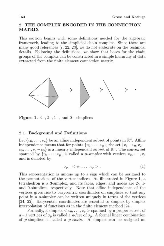
154 Gross and Kotiuga
2. THE COMPLEX ENCODED IN THE CONNECTIONMATRIX
This section begins with some definitions needed for the algebraicframework, leading to the simplicial chain complex. Since there aremany good references [7, 22, 23], we do not elaborate on the technicaldetails. Following the definitions, we show that bases for the chaingroups of the complex can be constructed in a simple hierarchy of dataextracted from the finite element connection matrix.
Figure 1. 3−, 2−, 1−, and 0− simplices
2.1. Background and Definitions
Let v0, . . . , vp be an affine independent subset of points in Rn. Affineindependence means that for points v0, . . . , vp, the set v1− v0, v2−v0, . . . , vp− v0 is a linearly independent subset of Rn. The convex setspanned by v0, . . . , vp is called a p-simplex with vertices v0, . . . , vpand is denoted by
σp =< v0, . . . , vp > . (1)
This representation is unique up to a sign which can be assigned tothe permutations of the vertex indices. As illustrated in Figure 1, atetrahedron is a 3-simplex, and its faces, edges, and nodes are 2-, 1-and 0-simplices, respectively. Note that affine independence of thevertices gives rise to barycentric coordinates on simplices so that anypoint in a p-simplex can be written uniquely in terms of the vertices[24, 22]. Barycentric coordinates are essential to simplex-by-simplexinterpolation of functions as in the finite element method [24].
Formally, a simplex < v0, . . . , vq > spanned by a proper subset ofq+1 vertices of σp is called a q-face of σp. A formal linear combinationof p-simplices is called a p-chain. A simplex can be assigned an
Data structures for finite elements 155
orientation which is induced by the permutation of vertex order in< v0, . . . , vp >, odd permutation giving negative orientation and evenpermutation giving positive orientation. The boundary of a p-simplexis the p− 1-chain which is the following alternating sum of p− 1-faces:
∂pσp = ∂(< v0, . . . , vp >) =p∑i=0
(−1)i < v0, . . . , vi−1, vi+1, . . . , vp > .
(2)
Note that< v0, . . . , vi−1, vi+1, . . . , vp > is the p-face opposite vertex vi.This definition can be used to find the boundary of a p-chain and, by(2) and direct calculation, one can verify that in general ∂p−1∂p(·) = 0,i.e. the boundary of the boundary of any chain is zero. The operator∂p determines a matrix of incidence of p−1-simplices with p-simplices;we will have more to say about this when discussing the coboundaryoperator in Section 3.2.
A simplicial complex K is a collection of simplices such that everyface of a simplex ofK is inK and the intersection of two simplices inKis a face of each of the simplices. For each p ≥ 0, the structure formedby taking p-chains with integer coefficients in a complex K is a finitelygenerated free abelian group Cp(K;Z) with basis all the p-simplices inK. This is called the p-chain group of K.
The connection between Cp(K) and Cp−1(K) is via the boundarymap. Defining the boundary map on a basis of Cp(K), the map extendsby linearity to a map
∂p : Cp(K)→ Cp−1(K) (3)
so that it is a homomorphism between the chain groups. Thus, on acomplex of dimension n the collection of abelian groups Ci(K;Z) andboundary homomorphisms give the sequence
0−→Cn(K) ∂n−→ · · · ∂p−→ Cp−1(K)∂p−1−→ · · · −→ C1(K) ∂1−→ C0(K)→ 0.
(4)
Since Im ∂p+1 ⊆ ker ∂p (∂p∂p+1(·) = 0), (4) defines the chain complexof K, denoted by (C∗(K), ∂) or simply C∗(K).
As described below, the finite element connection matrix containsthis basic algebraic structure. It is of interest because whileIm ∂p+1 ⊆ ker ∂p, in general Im ∂p+1 = ker ∂p and the part ofker ∂p not in the inclusion contains useful information formulatedconcisely via homology groups and the exact homology sequence asdescribed elsewhere [22]. However, the chain complex fits betweenthe data which is readily available from the finite element mesh and“higher” topological structures such as the homology groups and thefundamental group of K.
156 Gross and Kotiuga
2.2. From Connection Data to Chain Groups
In this paper, the prime example of the simplicial complex K isa tetrahedral finite element mesh, a tetrahedral discretization of amanifoldR in R3 with boundary. Below we show that bases of the chaingroups Ci(K) related to a tetrahedral mesh can be computed from theconnection matrix by “following the boundary homomorphism downthe chain complex”.
Consider an n-dimensional simplicial complex K with mn n-simplices and m0 vertices or 0-simplices. There is a total ordering ofthe vertices on the index set 0, . . . ,m0 − 1 called the global vertexordering. There is a partial ordering of vertices such that vertices of ap-simplex are locally ordered on 0, . . . , n. The connection matrix isthe following mn ×m0 matrix defined in terms of the global and localorderings:
Cin,jk =
1 if global vertex k is the jth local vertex of the ith n-simplex
0 otherwise.
(5)
For a 3-d finite element mesh, C3 is simply the connection matrix whichis the output of a mesh generator. In general, (5) also defines lowerdimensional subcomplexes, Cp, 0 ≤ p ≤ n, or p-skeletons of a mesh. Inany case, Ci3,jk is an m3 ×m0 matrix, but typically m3 = km0 wherek is approximately 5 to 6. Since a tetrahedron has four vertices, theconnection matrix C3 has 4m3 nonzero entries so that the matrix isvery sparse.
Because of sparsity, only the nonzero entries of the matrices Cpare stored in mp×(p+1) arrays such that the ith row gives the (global)indices of the vertices σ0,k which define the ith p-simplex:
Cip = σ0,k0 , . . . , σ0,kp (6)
where 0 ≤ i ≤ mp − 1 and mp is the number of p-simplices in themesh. This is an efficient way of storing (5), and in this form Cp alsoresembles a basis for the chain group Cp(K) (the notation intentionallytakes them to be the same). It must be emphasized that referring tothe nonzero entries of the matrix in a table of pointers to the globalvertex ordering gives computational efficiency and a direct link to themaps and definitions of Section 2.1.
Consider the following map which extracts the jth p-face of thekth (p+ 1)-simplex:
fj(σp+1,k) =< σ0,0, . . . , σ0,j , . . . , σ0,p+1 >, (7)
Data structures for finite elements 157
where 1 ≤ i ≤ mp, 1 ≤ k ≤ mp+1, 0 ≤ j ≤ p + 1, and σ0,j denotesthat vertex σ0,j is omitted. Note that j and k do not uniquely specifythe p-simplex since < σ0,0, . . . , σ0,j , . . . , σ0,p+1 > may be a p-face inmore than one (p+1)-simplex. The representation of the p-simplex byvertex ordering is unique up to orientation, but the orientation inducedfrom the (p + 1)-simplex can always be adopted in order to maintainconsistency. In any case, the map gives the p-faces of the p+1-simplexwhen used for 0 ≤ j ≤ p+ 1.
To build Cp, equation (7) can be used p+2 times on each (p+1)-simplex in Cp+1 (effectively taking the boundary of each p+1-simplex inCp+1). In each instance this requires that an algorithm which extractsthe p-simplices determine from the existing data for Cp whether theresult of applying (7) is a new p-simplex or one that has already beenextracted. Thus, starting with Cn, it is possible to go down the complex(4) and extract all the tables Cp.
Below is an algorithm which builds Cp from Cp+1. The algorithmvisits each p-face of every p + 1-simplex, or (p + 2)mp+1 applicationsof (7).
Algorithm 1 (Extraction of Cp from Cp+1)Set Cp to be empty.ForEach σp+1 ∈ Cp+1
ForEach p-face of σp+1
If p-face is not in CpThen add p-face to Cp.EndFor
Endfor
The decision at the inner loop requires a search through Cp butif implemented in an efficient data structure such as a linked list, thesearch is bounded by the number of times any vertex of the p-face is avertex in a p-simplex.
2.3. Considerations for Cellular Meshes
While we focus primarily on simplicial complexes, all of thealgebraic structure described is consistent for cellular complexes (e.g.,hexahedral meshes). In practice, the data structures are somewhatmore complicated because the vertices, while ordered on a cell, arenot generally permutable. This affects the definition of (7) so thatsome additional information about the ordering of vertices may haveto be preserved at every step of the algorithm. This also influencesthe way in which the algorithms are implemented — in particular,depending on application, it is most efficient to extract the 1- and
158 Gross and Kotiuga
2-complexes simultaneously, 3-cell by 3-cell, in order to avoid storingextra information about vertex ordering.
3. THE COCHAIN COMPLEX
In de Rham theory, integration on manifolds in Rn is formulated asan algebraic structure which pairs p-chains with differential p-forms.The algebras of differential p-forms are related in a (de Rham) complex,and the related (co)homology groups are the link between lumped fieldparameters and topological invariants of the manifold in question [13].An elaboration of this is given in Section 6. In the discrete setting (e.g.,triangulated manifolds), cochains play a role analogous to differentialforms and since simplicial (co)homology satisfies the same axioms asthe de Rham cohomology, the theories are equivalent [10]. In thissection we define cochains and their algebraic structure. The algebrais dual to the chain complex. Then we see how this structure alsocomes out of the connection matrix.
3.1. Simplicial Cochain Groups and the CoboundaryOperator
Formally, the simplicial p-cochain group Cp(X;Z) is the group ofhomomorphisms from p-chains to (for the present purpose) theintegers:
Cp(X;Z) = hom(Cp,Z). (8)
Cp(X;Z) is a Z-module and not a vector space, but one can regardthe homomorphisms as functionals on chains and denote the operationof a cochain cp ∈ Cp(X;Z) on a chain cp ∈ Cp(X;Z), by functionalnotation:
cp(cp) =< cp, cp > . (9)
The p-coboundary operator dp is the adjoint of the boundaryoperator. It is defined by
< dpcp, cp+1 >=< cp, ∂p+1cp+1 > . (10)
so that
dp = (∂p+1)T : Cp(X;Z) −→ Cp+1(X;Z). (11)
From this point the p-coboundary operator is always written explicitlyas the adjoint operator ∂Tp+1. Equation (10) is simply a discrete
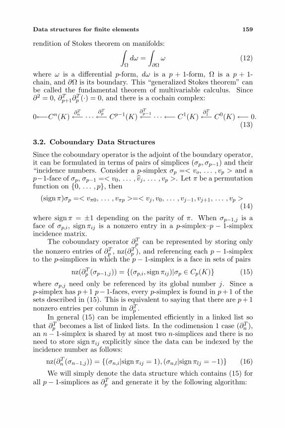
Data structures for finite elements 159
rendition of Stokes theorem on manifolds:∫Ωdω =
∫∂Ωω (12)
where ω is a differential p-form, dω is a p + 1-form, Ω is a p + 1-chain, and ∂Ω is its boundary. This “generalized Stokes theorem” canbe called the fundamental theorem of multivariable calculus. Since∂2 = 0, ∂Tp+1∂
Tp (·) = 0, and there is a cochain complex:
0←−Cn(K)∂Tn←− · · ·
∂Tp←− Cp−1(K)∂Tp−1←− · · · ←− C1(K)
∂T1←− C0(K)←− 0.(13)
3.2. Coboundary Data Structures
Since the coboundary operator is the adjoint of the boundary operator,it can be formulated in terms of pairs of simplices (σp, σp−1) and their“incidence numbers. Consider a p-simplex σp =< vo, . . . , vp > and ap−1-face of σp, σp−1 =< v0, . . . , vj , . . . , vp >. Let π be a permutationfunction on 0, . . . , p, then
(signπ)σp =< vπ0, . . . , vπp >=< vj , v0, . . . , vj−1, vj+1, . . . , vp >(14)
where signπ = ±1 depending on the parity of π. When σp−1,j is aface of σp,i, signπij is a nonzero entry in a p-simplex–p − 1-simplexincidence matrix.
The coboundary operator ∂Tp can be represented by storing onlythe nonzero entries of ∂Tp , nz(∂Tp ), and referencing each p − 1-simplexto the p-simplices in which the p− 1-simplex is a face in sets of pairs
nz(∂Tp (σp−1,j)) = (σp,i, signπij)|σp ∈ Cp(K) (15)
where σp,j need only be referenced by its global number j. Since ap-simplex has p+1 p− 1-faces, every p-simplex is found in p+1 of thesets described in (15). This is equivalent to saying that there are p+1nonzero entries per column in ∂Tp .
In general (15) can be implemented efficiently in a linked list sothat ∂Tp becomes a list of linked lists. In the codimension 1 case (∂Tn ),an n− 1-simplex is shared by at most two n-simplices and there is noneed to store signπij explicitly since the data can be indexed by theincidence number as follows:
nz(∂Tn (σn−1,j)) = (σn,i|signπij = 1), (σn,l|signπlj = −1) (16)
We will simply denote the data structure which contains (15) forall p− 1-simplices as ∂Tp and generate it by the following algorithm:
160 Gross and Kotiuga
Algorithm 2. (Construction of ∂Tp )Set ∂Tp to be empty.ForEach σp−1 ∈ Cp−1 (mp−1 p− 1-simplices)
ForEach σp such that signπij = 0augment list for σp−1 with (σp, signπ).
EndForEndFor
At first sight, the inner loop of algorithm 2 seems to require asearch through all of the Cp data structure for each case where σp−1 isa p − 1-face. In practice the searching can be avoided by performingthe augmentation procedure each time the p−1-simplex is encounteredin the inner loop of algorithm 1. With an efficient data structureimplementation, reaching the point where the ∂Tp list is augmented isbounded by the number of times σp is a p-face.
4. APPLICATION: WHITNEY FORMS
Recent years have seen the growing use of so-called Whitney 1-forms oredge elements for a variety of finite element computations. The generalidea comes from Whitney [27, 26] and was developed in [9, 21] to whichwe refer for proofs. It starts with a linear Whitney map which makespiecewise linear differential q-forms from simplicial q-cochains:
W : Cq(K)→ L2Λq(X) (17)
where X is a compact oriented C∞ Riemannian manifold of dimensionn, L2Λq(X) is the space of square-integrable de Rham C∞ differentialq-forms on X, and K is a simplicial triangulation of X. Let µi bebarycentric coordinates corresponding to vertices vi in K. The basicform Wσ ∈ L2Λq(X) on a q-simplex σ, is defined as
Wσ = q!∑q
k=0(−1)kµik dµi0 ∧ . . . ∧ dµik ∧ . . . ∧ dµiq q > 0W (vi) = µi q = 0
(18)
where ∧ denotes the wedge product for differential forms and, as inSection 2.2, · denotes that the differential is excluded. Note thatthe construction of this q-form corresponds neatly to the process ofextracting q− 1-simplices from q-simplices in Section 2.2. We mentiontwo properties of the Whitney map:
(i) W∂T c = dWc for c ∈ Cq(K) where ∂T c ∈ Cq+1(K) is thesimplicial coboundary of c. The exterior derivative d : Λq → Λq+1
applied to Wc is well-defined in this case.
Data structures for finite elements 161
(ii) Let < , > denote the pairing of Cq(K) and Cq(K) as in (9). Then∫cq
Wcq =< cq, cq > (19)
for every cochain cq ∈ Cq and chain cq ∈ Cq(K).
The first property is significant because it implies that the simplicialcohomology groups of K and the de Rham cohomology group of X(see Section 6) are isomorphic.
In addition to the Whitney map (17), there is a de Rham map
R : L2Λq(X)→ Cq(K) (20)
which is defined on a basis of chains by∫cq
ω =< cq, cq > (21)
and the second property of the Whitney map ensures that
RW = I (22)
where I is the identity map. The convergence WR → I as a mesh isrefined is a special case of both finite element theory and Whitney’sprogram, but this obvious connection does not seem to exist outsideof computational electromagnetics and the work of Dodziuk [8, 9] andMuller [21].
For c, c′ ∈ Cq(K), an inner product can be defined:
(c, c′) =∫XWc ∧ ∗Wc′ = (Wc,Wc′). (23)
This is nondegenerate by the property of the de Rham map. Althoughthere is no obvious metric inherent to the simplicial complex K, thisinner product inherits a metric from X through the Whitney map. Asa mesh is refined, the inherited metric in the inner product convergesto the (Riemannian) metric on X.
4.1. Example: The Helicity Functional
For finite element computations of magnetic fields, a Whitney 1-formcan be used to discretize the magnetic field intensity. Namely,
ω = H · dr. (24)
162 Gross and Kotiuga
Then, on a 1-simplex,
hij =∫ vj
vi
ω (25)
define the variables of a 1-cochain for ω. In this formulation, it isinteresting to note that the contribution of the so-called helicity densityω∧dω to the finite element “stiffness” matrix is independent of metricand constitutive laws [15]. In particular, the contribution of the helicityon a tetrahedron to the stiffness matrix is
12
∫σ3
ω ∧ dω =16(h01h23 − h02h13 + h03h12) (26)
The righthand side is a quadratic form which remains invariant bythe action of the Lie group SL(4,R) associated with piecewise linearvolume-preserving diffeomorphisms.
5. THE DUAL COMPLEX AND DISCRETE POINCAREDUALITY FOR (CO)CHAINS
One reason for developing the coboundary data structures is to makeuse of a duality relation which relates cochains of the simplicial complexK to chains on the dual complex of K. A thorough developmentof the dual chain complex of K (c.f. [22]) usually starts with thefirst barycentric subdivision of K and construction of “blocks” in thesubdivision which are dual to the p-simplices of K where the dualblocks are unions of certain sets of open simplices in the subdivision.
Although the definition of the dual complex [22] relies on somegeometry, the incidence data for the dual complex can be recoveredfrom the coboundary data structures of the simplicial complex [25], sowe will formally define the dual chain complex DK with the followingconstruction. The dual complex of a simplicial complex K, is a cellcomplex DK obtained by identifying p-simplices on K with (n − p)-cells. In general DK is not a simplicial complex, so it is necessaryto use the terminology of cells. However it is possible to formulate acomplex C∗(DK) as previously done for K in (4).
In explicit terms, we identify 3-simplices with 0-cells (vertices ofDK), 2-simplices with 1-cells (edges), 1-simplices with 2-cells (faces)and 0-simplices with 3-cells. Since the coboundary data structuresalready contain the incidence of p-simplices in p + 1-simplices, thesecan be reinterpreted on the dual complex as the boundaries of n − p-cells. For example, the entries of (16) can be regarded as the 0-cellsincident to a 1-cell in DK which passes “through” the barycenter of
Data structures for finite elements 163
σ2,j . Equation (15) is interpreted as the boundaries of 2- and 3-cells(∂T1 and ∂T2 respectively) in DK associated with (3− 2)- and (3− 3)-simplices, respectively, in K.
A useful form of Poincare duality formalizes the connectionbetween ∂Tp and boundaries of (n − p)-cells in DK seen in the datastructures. It establishes a duality between cochains in K and chainsinDK. While the complexes Cp(K) and Cp(K) are duals by definition,there exists a nondegenerate bilinear “intersection pairing”
I : Cp(DK)× Cn−p(K) −→ R. (27)
This leads to the duality
Cp(DK) ∼= Cn−p(K) (28)
since both are duals of Cn−p(K) [22]. Comparison of the chaincomplexes C∗(K) and C∗(DK) in light of this duality says thatboundary and coboundary operators can be identified:
∂Tp+1 = ∂n−p (29)
where ∂ denotes the boundary operator on DK. The sameidentification is seen in the data structures. Hence, for the price ofextracting the cochain complex from the connection matrix, we havelearned everything about the dual chain complex.
6. APPLICATIONS: SIMPLICIAL (CO)HOMOLOGYAND CUTS FOR SCALAR POTENTIALS
So far we have spelled out the simplicial consequences of the finiteelement connection matrix. In this section we look at two applicationsof simplicial (co)chain complexes and Poincare duality to see how theybeneficial in 3-d finite element computation.
6.1. Simplicial (Co)Homology
The chain complex is readily available from the connection matrix,but for many purposes it is merely the starting point. In this sectionwe consider how homology groups follow from the chain complexand see how they algebraically expose the lumped parameters ofelectrical engineering (e.g., current, voltage, flux) which come aboutfrom integration on p-chains.
For the boundary homomorphism ∂p in equation (3), we callker ∂p = Zp(K) the p-cycles in K and Im ∂p+1 = Bp(K) the p-boundaries in K. Both Zp(K) and Bp(K) are subgroups of Cp(K),
164 Gross and Kotiuga
and furthermore, Bp(K) ⊆ Zp(K) ⊂ Cp(K). This is true since ifβ ∈ Bp(K) then β = ∂p+1α, for some α ∈ Cp+1(K), but ∂p∂p+1α = 0says that β ∈ ker ∂p, i.e., β ∈ Bp(K).
In general it is interesting to ask when is a p-cycle not a p-boundary. This information is summarized in the pth simplicialhomology group of K, p ≥ 0, defined as the quotient group
Hp(K) =Zp(K)Bp(K)
=ker ∂p
Im ∂p+1. (30)
This quotient group consists of equivalence classes of cycles c such that∂c = 0 but c is not a boundary. Two p-cycles a and b are in the sameequivalence class if they satisfy the equivalence relation:
[a] ∼ [b]⇐⇒ a− b = ∂cp+1, (31)
where c is p + 1-chain and [a] denotes the homology class of a. Therank of Hp(K) is the number of independent equivalence classes in thegroup and is known as the pth Betti number of K, denoted by βp(K);intuitively, β0(K) counts the number of connected components of K,and β1(K) counts the “number of holes in K” [20, 12, 11].
Calling Zp(X;Z) = ker ∂Tp the group of p-cocycles, andBp(X;Z) = Im ∂Tp−1 the group of p-coboundaries, the pth cohomologygroup is:
Hp(X;Z) =Zp(X;Z)Bp(X;Z)
=ker ∂Tp+1
Im ∂Tp. (32)
To make the connection with lumped parameters, we also need tointroduce relative homology groups. Let L be a subcomplex of K, thatis a simplicial complex contained in K. Then the pth relative simplicialhomology group of K “modulo” L is
Hp(K,L;Z) = Hp(C∗(K)/C∗(L);Z), (33)
that is, the homology of the quotient of the two complexes. Inparticular, if L = ∂K, two p-cycles from an equivalence class inHp(K, ∂K) form a p-boundary in K when taken in combination with ap-chain in ∂K. Relative cochains (with integer coefficients) are definedby
Cp(K,L;Z) = hom(Cp(K,L),Z) (34)
so that the pth relative cohomology group is
Hp(K,L;Z) =ker ∂Tp
Im ∂Tp+1
(35)
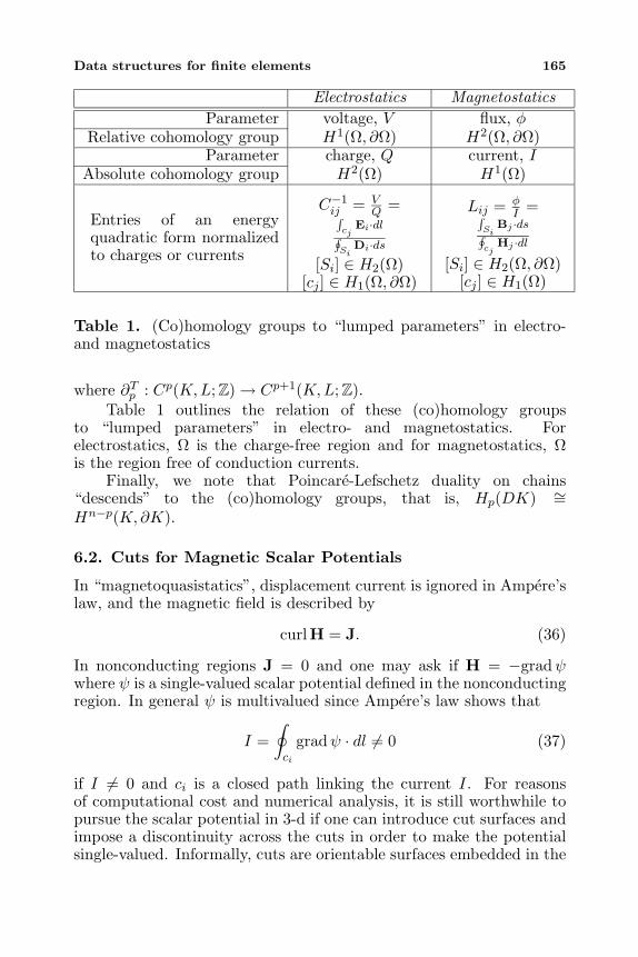
Data structures for finite elements 165
Electrostatics MagnetostaticsParameter voltage, V flux, φ
Relative cohomology group H1(Ω, ∂Ω) H2(Ω, ∂Ω)Parameter charge, Q current, I
Absolute cohomology group H2(Ω) H1(Ω)
Entries of an energyquadratic form normalizedto charges or currents
C−1ij = V
Q =∫cj
Ei·dl∮Si
Di·ds[Si] ∈ H2(Ω)
[cj ] ∈ H1(Ω, ∂Ω)
Lij = φI =∫
SiBj ·ds∮
cjHj ·dl
[Si] ∈ H2(Ω, ∂Ω)[cj ] ∈ H1(Ω)
Table 1. (Co)homology groups to “lumped parameters” in electro-and magnetostatics
where ∂Tp : Cp(K,L;Z)→ Cp+1(K,L;Z).Table 1 outlines the relation of these (co)homology groups
to “lumped parameters” in electro- and magnetostatics. Forelectrostatics, Ω is the charge-free region and for magnetostatics, Ωis the region free of conduction currents.
Finally, we note that Poincare-Lefschetz duality on chains“descends” to the (co)homology groups, that is, Hp(DK) ∼=Hn−p(K, ∂K).
6.2. Cuts for Magnetic Scalar Potentials
In “magnetoquasistatics”, displacement current is ignored in Ampere’slaw, and the magnetic field is described by
curlH = J. (36)
In nonconducting regions J = 0 and one may ask if H = −gradψwhere ψ is a single-valued scalar potential defined in the nonconductingregion. In general ψ is multivalued since Ampere’s law shows that
I =∮ci
gradψ · dl = 0 (37)
if I = 0 and ci is a closed path linking the current I. For reasonsof computational cost and numerical analysis, it is still worthwhile topursue the scalar potential in 3-d if one can introduce cut surfaces andimpose a discontinuity across the cuts in order to make the potentialsingle-valued. Informally, cuts are orientable surfaces embedded in the
166 Gross and Kotiuga
current-free region such that when integrating H · dl around a closedpath which links current, the path must pass through the cuts. Cutscoincide with the flux measurement surfaces Si in the right column oftable 1 [11].
The existence of cuts as compact, embedded, orientable manifoldsin R can be formulated via a constructive proof which gives analgorithm for computing them on finite element meshes which aretriangulations of the nonconducting region [14]. There are many facetsto the algorithm, but here we touch on only one. The first step tocomputing a set of cuts for a mesh is to compute a set of topologicalconstraints which represent a set of generators for classes inH2(K, ∂K)[11]. By the Poincare-Lefschetz duality of Section 4 this problem canbe phrased as finding a basis for classes in H1(DK), and reduces tofinding a basis of the nullspace of ∂T2 , or a set of vectors ζ1, . . . ζβ1satisfying
∂T2 ζi = 0 (38)
subject to Im ∂T0 = 0 [11]. The problem is motivated strictlyby topological considerations at every step and requires the datastructures C3, C2, ∂T3 , ∂T2 , ∂T1 of Sections 2 and 3 and the dualityof Section 4 for the computation.
7. CONCLUSION
Once a tetrahedral finite element mesh is identified as the triangulationof a 3-manifold with boundary, simplicial complexes give a systematicand general way for creating and organizing finite element datastructures. The simplicial chain and cochain complexes are the bridgebetween the topology of the manifold, vector fields in the region, andstructures from algebraic topology which are useful for finite elementcomputation. The data structures are the most natural for usingWhitney elements, in particular Whitney edge elements. Helicityfunctionals and cuts for magnetic scalar potentials are good examplesof applications where the metric of the space and the topology can beseparated. In these contexts, the data structures provide a high degreeof computational efficiency.
ACKNOWLEGMENT
P. Gross gratefully acknowledges support received from the NationalScience Foundation, grant INT-9600286.
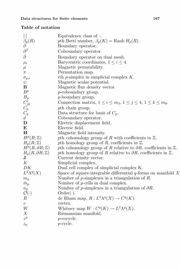
Data structures for finite elements 167
Table of notation
[·] Equivalence class of ·.βp(R) pth Betti number, βp(K) = Rank Hp(R).∂ Boundary operator.∂T Coboundary operator.∂ Boundary operator on dual mesh.µi Barycentric coordinates, 1 ≤ i ≤ 4.µ Magnetic permeability.π Permutation map.σp,i ith p-simplex in simplicial complex K.ψ Magnetic scalar potential.B Magnetic flux density vector.Bp p-coboundary group.Bp p-boundary group.Cijk Connection matrix, 1 ≤ i ≤ m3, 1 ≤ j ≤ 4, 1 ≤ k ≤ m0.Cp pth chain group.Cp Data structure for basis of Cp.d Coboundary operator.D Electric displacement field.E Electric field.H Magnetic field intensity.Hp(R;Z) pth cohomology group of R with coefficients in Z.Hp(R;Z) pth homology group of R, coefficients in Z.Hp(R, ∂R;Z) pth cohomology group of R relative to ∂R, coefficients in Z.Hp(R, ∂R;Z) pth homology group of R relative to ∂R, coefficients in Z.J Current density vector.K Simplicial complex.DK Dual cell complex of simplicial complex K.L2Λq(X) Space of square-integrable differential q-forms on manifold X.mp Number of p-simplexes in a triangulation of R.mp Number of p-cells in dual complex.np Number of p-simplexes in a triangulation of ∂R.O(·) Order(·).R de Rham map, R : L2Λq(X)→ Cq(K).v vertex.W Whitney map W : Cq(K)→ L2Λq(X).X Riemannian manifold.zp p-cocycle.zp p-cycle.
168 Gross and Kotiuga
REFERENCES
1. Balabanian, N. and T. A. Bickart, Electrical Network Theory, 80,John Wiley and Sons, New York, 1969.
2. Bamberg, P. and S. Sternberg, A Course in Mathematics forStudents of Physics: 2, Ch. 12, Cambridge U. Press, NY, 1990.
3. Bossavit, A., Computational Electromagnetism, VariationalFormulations, Edge Elements, Complementarity, Academic Press,Boston, 1997.
4. Brisson, E., “Representing geometric structures in d dimensions:Topology and order,” Discrete and Computational Geometry,Vol. 9, 387–426, 1993.
5. Brown, M. L., “Scalar potentials in multiply connected regions,”Int. J. Numer. Meth. Eng., Vol. 20, 665–680, 1984.
6. Chammas, P. and P. R. Kotiuga, “Sparsity vis a vis Lanczosmethods for discrete helicity functionals,” Proc. of the ThirdInt. Workshop on Electric and Magnetic Fields, A. Nicolet andR. Belmans (eds.), 1996.
7. Croom, F. H., Basic Concepts of Algebraic Topology, Chaps. 2,7.3, 4.5, Springer-Verlag, New York, 1978.
8. Dodziuk, J., “Combinatorial and continuous hodge theories,” Bull.AMS, Vol. 80, 1014–1016, 1974.
9. Dodziuk, J., “Finite-difference approach to the hodge theory ofharmonic forms,” Am. J. Math., Vol. 98, 79–104, 1976.
10. Eilenberg, S. and N. Steenrod, Foundations of Algebraic Topology,Princeton University Press, Princeton, New Jersey, 1952.
11. Gross, P. W. and P. R. Kotiuga, “Finite element-based algorithmsto make cuts for magnetic scalar potentials: Topologicalconstraints and computational complexity,” this volume.
12. Gross, P. W. and P. R. Kotiuga, “A challenge for magneticscalar potential formulations of 3-d eddy current problems:Multiply connected cuts in multiply connected regions whichnecessarily leave the cut complement multiply connected,” Electricand Magnetic Fields: From Numerical Models to IndustrialApplications, A. Nicolet and R. Belmans (eds.), 1–20, New York,1995. Proc. of the Second Int. Workshop on Electric and MagneticFields.
13. Kotiuga, P. R., “Hodge decompositions and computationalelectromagnetics,” Ph.D. thesis, 123, McGill University, Montreal,1984.
14. Kotiuga, P. R., “An algorithm to make cuts for scalar potentials
Data structures for finite elements 169
in tetrahedral meshes based on the finite element method,” IEEETrans. Magn., Vol. 25, 4129–4131, 1989.
15. Kotiuga, P. R., “Helicity functionals and metric invariance in threedimensions,” IEEE Trans. Magn., Vol. 25, 2813–2815, 1989.
16. Kotiuga, P. R., “Analysis of finite-element matrices arising fromdiscretizations of helicity functionals,” J. Appl. Phys., Vol. 67,5815–5817, 1990.
17. Kotiuga, P. R., “Topological duality in three-dimensional eddy-current problems and its role in computer-aided problemformulation,” J. Appl. Phys., Vol. 67, 4717–4719, 1990.
18. Kotiuga, P. R., “Essential arithmetic for evaluating threedimensional vector finite element interpolation schemes,” IEEETrans. Magn., Vol. MAG-27, 5208–5210, 1991.
19. Kron, G., “Basic concepts of multidimensional space filters,”AIEE Trans., Vol. 78, 554–561, 1959.
20. Maxwell, J. C., A Treatise on Electricity and Magnetism (1891),Chap. 1, Art. 18–22, Dover, New York, 1954.
21. Muller, W., “Analytic torsion and r-torsion of riemannianmanifolds,” Advances in Mathematics, Vol. 28, 233–305, 1978.
22. Munkres, J. R., Elements of Algebraic Topology, 377–380,Addison-Wesley, Reading, MA, 1984.
23. Rotman, J. J., An Introduction to Algebraic Topology, Springer-Verlag, NY, 1988.
24. Silvester, P. and R. Ferrari, Finite Elements for ElectricalEngineers, 2nd Ed., Cambridge U. Press, NY, 1990.
25. Whitney, H., “On matrices of integers and combinatorialtopology,” Duke Math. J., Vol. 3, 35–45, 1937.
26. Whitney, H., “r-Dimensional integration in n-space,” Proc. of theInt. Congress of Mathematicians, Vol. 1, 1950.
27. Whitney, H., Geometric Integration Theory, Princeton UniversityPress, Princeton, New Jersey, 1957.
Progress In Electromagnetics Research, PIER 32, 171–188, 2001
GEOMETRIC ASPECTS OF THE SIMPLICIALDISCRETIZATION OF MAXWELL’S EQUATIONS
F. L. Teixeira†
Research Laboratory of ElectronicsDepartment of Electrical Engineering and Computer ScienceMassachusetts Institute of TechnologyCambridge, MA 02139-4307, USA
Abstract—Aspects of the geometric discretization of electromagneticfields on simplicial lattices are considered. First, the convenience ofthe use of exterior differential forms to represent the field quantitiesthrough their natural role as duals (cochains) of the geometricconstituents of the lattice (chains = nodes, edges, faces, volumes)is briefly reviewed. Then, the use of the barycentric subdivisionto decompose the (ordinary) simplicial primal lattice together withthe (twisted) non-simplicial barycentric dual lattice into simplicialelements is considered. Finally, the construction of lattice Hodgeoperators by using Whitney maps on the first barycentric subdivisionis described. The objective is to arrive at a discrete formulation ofelectromagnetic fields on general lattices which better adheres to theunderlying physics.
1 Introduction1.1 Outline
2 Discretization of the Topological Equations2.1 Simplicial Lattices and Complexes2.2 Pairing and Incidence Matrices2.3 Complexes and Orientation
3 Discretization of the Metric Equations3.1 Discrete Hodge Operators3.2 Whitney and de Rham Maps
† Present address: ElectroScience Laboratory and Department of Electrical Engineering,1320 Kinnear Road, The Ohio State University, Columbus, OH 43212-1191, USA
172 Teixeira
4 Dual Lattices and Barycentric Subdivision4.1 Hodge Duality in Topological Field Theories4.2 Whitney Maps on the Dual Lattice via Barycentric
Subdivision
5 Conclusions
References
1. INTRODUCTION
Like most equations of physics, Maxwell’s equations are extremely richin symmetries and (hence) conservation laws. In the continuum, manyconservation laws follow directly from invariances of the Lagrangian(Noether symmetries) such as energy or momentum conservation, whileothers have an inherent topological aspect, such as magnetic charge.However, when Maxwell’s equations are discretized on a lattice, anumber of symmetries of the continuum theory are modified or broken.Still, many conservation laws may be trivially preserved on a discretesetting. This is because they often relate a quantity on certain region ofspace to an associated quantity on the boundary of the region. Becausethe boundary is a topological invariant, such conservation laws shouldnot depend on the metric of the space (i.e., they are invariant underhomeomorphisms). As a result they are also scale invariant and shouldnot depend (in a consistent discrete model of the theory) whethera continuum limit is taken. A natural mathematical language thatexplore this aspect is the calculus of exterior differential forms [1–45]and associated algebraic topological structures [1–12, 15–21, 23–29, 32,35–38, 40–45].
This is partly because, when cast in such language, Maxwell’sequations are factorized into a purely topological (i.e., metric-free) part
dE = − ∂
∂tB (1)
dH =∂
∂tD + J (2)
dB = 0 (3)dD = ρ (4)
and a metric dependent part
D = εE (5)B = µH (6)
Geometric aspects of simplicial discretization 173
In the above, E and H are electric and magnetic field intensity 1-forms,D and B are electric and magnetic flux density 2-forms, J is the electriccurrent density 2-form, and ρ is the electric charge density 3-form. Themetric-free operator d is the exterior derivative, which simultaneouslyplays the role of the grad, curl, and div operators of vector calculus,distilled from their metric structure. Constitutive parameters of agiven medium in Eqs. (5) and (6) relate the 1-forms E, H to the 2-forms D, B and are given in terms of the so-called Hodge operators, εand µ, which also include all metric information [13, 26, 28, 32, 33,36, 38–40, 48].
This is unlike the vector calculus formalism, where metricand topological structures are intertwined in the equations. Asalluded, such factorization has important consequences (even in thetopologically trivial manifolds of interest) if the objective is to arriveat a consistent discretization scheme for Maxwell’s equations in generallattices. There are many reasons for that. First, the topologicalequations (1)–(4) admit an exact discrete spatial rendering [40].Therefore, many theorems (such as charge conservation alluded before)are automatically fullfilled after discretization, without the need toinvolve metric concepts. Second, because the metric is completelyencoded into Eqs. (5) and (6), the treatment of curved boundaries andmaterial interfaces [also entirely encoded in Eqs. (5) and (6)] can bedone in a more systematic manner, without affecting, e.g., conservationlaws related to the topological equations. Third, once discretized,the topological (spatial) part of the equations often comprises integerarithmetic only and are more efficiently handled by a computer if apriori recognized as such1.
Besides this natural factorization, the language of forms alsosheds light in a number of issues faced by various discretizationmethods. Among them are rationale for the use of edge (Whitney)elements in finite element methods [19, 23, 35] (related with the correctinterpolation of the electric and magnetic field intensities 1-forms Eand H) and for the dual grid construction in finite difference and finitevolume methods [10, 32, 40] (related with the concept of external andinternal orientations of differential forms).
1.1. Outline
In this paper, we first review the terminology and basic conceptsof the spatial discretization of Maxwell’s equations using discretedifferential forms (cochains), with special emphasis on the factorization1 Exceptions to this last point are lattices involving some sort of spatial interpolation forthe boundary stencil, such as in many subgridding or locally conformal grid situations.
174 Teixeira
of the topological and metric problems. We then discuss morespecific geometric aspects of the discretization using a simplicalprimal lattice and a non-simplicial barycentric dual lattice as startingpoint, followed by a barycentric subdivision (decomposition) of boththese lattices. Motivated by the results in [45] and through therepresentation of the cochains (electromagnetic fields) via Whitneyforms, the first barycentric subdivision is then used as the actualtool for discretization. The objectives are to arrive at a coordinate-free, discrete version of Maxwell’s equations for general lattices withfewer ad-hoc interpolatory rules, and to have the geometric structure ofthe continuum theory mirrored, to a maximum extent, by its discretecounterpart.
2. DISCRETIZATION OF THE TOPOLOGICALEQUATIONS
2.1. Simplicial Lattices and Complexes
Simplicial lattices will be considered here not only because of theirflexibility in dealing with complex geometries, but also because theyare more fundamental in the sense that any lattice can be built byassembling simplicial elements. For our purposes, the term simpliciallattice will refer to a simplicial complex embedded on a Euclidean, E3
space (i.e., with a metric structure associated to it).For completeness, we will next briefly sketch the definition of
simplicial complex. More detailed descriptions can be found elsewhere,e.g., [1, 4, 5, 6, 7, 40, 45].
Given x0, x1, ...xM affine points in an abstract space, a M -simplex,σM , is the set of points (convex hull) given by x =
∑Mi=0 λixi where λi
are the barycentric coordinates such that∑Mi=0 λi = 1 and λi ≥ 0. We
write σM = [x0, x1, ...xM ]. In a three-dimensional space, a 0-simplexis a point, a 1-simplex is an edge (line segment), a 2-simplex is a face(triangle), and a 3-simplex is a volume (tetrahedron). An orientedM -simplex changes sign under a change of orientation, i.e., if σM =[x0, x1, ...xM ] and a permutation of the indices is carried out, then[xτ(0), xτ(1), ...xτ(M)] = (−1)τσM , where τ denotes the total numberof permutations needed to restore the original index order (odd oreven permutations). The j-face of a simplex is the set defined byλj = 0. The faces of a 1-simplex [x0, x1] are the points [x0] and [x1](0-simplices), the faces of a 2-simplex [x0, x1, x2] are its three edges,i.e., [x0, x1], [x1, x2], and [x0, x2] (1-simplices), and so forth. We denotethe simplex σMi as being a face of the simplex σM
′j , with M < M ′, by
Geometric aspects of simplicial discretization 175
σMi ⊂ σM′
j .A simplicial complex χ is a collection of simplices such that (i)
for all σM belonging to χ, its faces also belong to χ, and (ii) forany two simplices their intersection is either empty or it is a commonface of both. We note that the concept of simplicial complex (and ofbarycentric coordinates) is independent of a metric and therefore willconstitute the general structure over which the discretized version ofEqs. (1)–(4) will be cast. Only Eqs. (5) and (6) will make use of themetric structure to be introduced a posteriori. When the elementsare not necessarily simplicial (e.g, Yee’s tetrahedral cells), we have acell complex, and its elements are called cells. A simplicial complex istherefore a particular case of a cell complex.
In the continuum, a natural duality exists between exteriordifferential forms and regions of integration (points, lines, surfaces,volumes) [1, 2, 13, 15, 23, 40, 60]. Indeed, integrals can be thoughas a pairing (contraction) of differential forms with these geometricalobjects which gives a scalar as a result. On a lattice or cell complex,the geometrical objects will be formal sums of simplices, called chains.A M -chain is a linear combination of M -simplices in χ through ΩM =∑i αiσ
Mi ∈ χ, with coefficients αi over the reals (for our purposes).
From this definition, a 0-chain is a linear combination of points, a 1-chain is a linear combination of edges (lines), etc. A chain is alwaysone of these types (there are no mixed chains) and the M -simplices σM(or M -cells in general) form a basis for the space of M -chains, CM .
2.2. Pairing and Incidence Matrices
Given an arbitrary simplicial complex, Eqs. (1)–(4) are easilydiscretized through a pairing with corresponding elements of twocomplexes χ and χ, and by using the adjoint of the exterior derivatived. On a lattice, the operator d is referred as the coboundary operatorwhose adjoint is called the boundary operator ∂ [32, 40, 45]. Theboundary operator carries its usual intuitive meaning [14]. Eqs. (3)and (4) are trivially verified on a lattice from the nilpotency of theboundary operator, ∂2 = 0 (i.e., the topological fact that the boundaryof a boundary is zero). The topological Eqs. (1)–(4) on a complex arewritten as
∑j
βij〈σ1j , E〉 = − ∂
∂t〈σ2i , B〉 (7)
∑j
βij〈σ1j , H〉 = − ∂
∂t〈σ2i , D〉+ 〈σ2
i , J〉 (8)
176 Teixeira
∑j
γij〈σ2j , B〉 = 0 (9)
∑j
γij〈σ2j , D〉 = 〈σ3
i , ρ〉 (10)
The incidence matrices αij , βij , γij (and αij , βij , γij) in the aboveequations are the discrete representation of the operator ∂ in agiven complex χ (and χ). The incidence matrices are operationallydefined by the action of the boundary operator on a basis of 1-, 2-and 3-chains (i.e., simplices), σ1
i , σ2i σ3
i , respectively, through∂σ1
i =∑j αijσ
0j , ∂σ
2i =
∑j βijσ
1j , ∂σ
3i =
∑j γijσ
2j , ∂σ
1i =
∑j αij σ
0j ,
∂σ2i =
∑j βij σ
1j , and ∂σ3
i =∑j γij σ
2j [40]. These matrices are the
discrete counterparts to the grad, curl, and div operators, respectively,distilled from their metric structure. In the case of simplicial complexes(or any cell complex where the definition of the boundary stencil doesnot involve spatial interpolations), the elements of those matrices areintegers having the values ±1 (depending on the relative orientation)when σ
(k−1)j ∈ ∂σki , and zero otherwise (hence it involves only integer
arithmetic).The incidence matrices should obey a number of (consistency)
properties as discussed, e.g., in [40]. These properties are importantto assure that key theorems of the continuum theory (e.g., chargeconservation, reciprocity) are preserved in the discrete setting.Violation of those properties often result in clear nonphysical behaviorand harmful numerical artifacts such as unconditional instabilities.Because any metric structure is still irrelevant at this level ofdescription, these properties are classified as topological consistencyproperties. For simple, regular lattices, they are almost automaticallyfulfilled in the most usual discretization schemes. However, in latticeswith more involved topological structures, e.g., those involving someform of subgridding or conformal gridding, special care should be takento avoid violation of these properties under naive discretization schemes[40].
The discrete fields in Eqs. (7)–(10), counterpart to the differentialforms fields in Eqs. (1)–(4), are called cochains to stress that theybelong to the dual space of the chains of the cell complex, i.e.,CM . Cochains therefore constitute the discrete representation of theelectromagnetic fields. The map from the space of M-forms ΦM to thespace of M-cochains, CM is called the de Rham map, Rh : ΦM → CM .In the following, we will often use the terms cochains and formsinterchangeably to reflect that cochains are just discrete differentialforms.
Geometric aspects of simplicial discretization 177
2.3. Complexes and Orientation
The choice of two distinct complexes, χ for Eqs. (7) and (9) andχ for Eqs. (8) and (10), is not arbitrary. Instead, it is rooted ondistinct geometrical properties of the differential forms in Eqs. (1) and(3) versus those in Eqs. (2) and (4), and related to the concept oforientation [32, 40]. This is because while E and B (associated withenergy) possess internal orientation (ordinary forms or cochains), Dand H (associated with sources J and ρ) possess external orientation(twisted forms or cochains) [3, 40]. Because of this difference ongeometric properties, they are associated with different complexesinheriting these two types of orientation (i.e., ordinary forms to aordinary complex, and twisted forms to a twisted complex). This isindeed the geometrical reason behind the dual lattice construction inmany finite volume and finite difference methods [32]. Here, we willchoose the simplicial primal complex as the ordinary complex and thedual cell complex as the twisted complex. The reciprocal choice couldbe made as well.
3. DISCRETIZATION OF THE METRIC EQUATIONS
The discretization of the topological equations provide a counterpart tothe continuum equations, Eqs. (1)–(4). In contrast, the discretizationof the metric equations provides an approximation of the continuumequations, Eqs. (5), (6). Error analysis may focus on the metric partof the equations.
3.1. Discrete Hodge Operators
Equations (5) and (6) generalize the constitutive equations andincorporate all metric information about a particular lattice. In thecontinuum, the Hodge operators relate M -forms with (N −M) forms,where N is the dimension of the space. It establishes an isomorphismbetween these two spaces. In the discrete case, the discrete version ofthe Hodge operators ε and µ establish a map between the M -cochainson the primal, ordinary complex χ with the (N −M)-cochains on thedual, twisted complex χ and vice-versa, i.e.,
[ε] : C1(χ)→ C2(χ)
〈σ2i , D〉 =
∑j
[ε]ij 〈σ1j , E〉 (11)
[µ] : C1(χ)→ C2(χ)
178 Teixeira
〈σ2i , B〉 =
∑j
[µ]ij 〈σ1j , H〉 (12)
Discrete Hodge operators approximate the continuum Hodge operators[26]. Discretization methods usually yield procedural equivalent‘Hodge operators’ through quadratures rules and interpolations. Fromthe material properties of the background medium and from the metricproperties of the lattice (or equivalently, of the manifold where thelattice is assumed embedded), the discrete Hodge operators shouldexhibit some key basic properties in order to lead to a consistent(in the sense of [40]) discrete theory. For example, in the case ofa reciprocal medium and on the usual Euclidean space, the discreteHodge operators should necessarily be symmetric, positive definiteoperators [40].
In order to obtain an explicit time-update scheme in the case ofa time domain method, at least one of the matrices in Eqs. (11),(12) needs to be diagonal. In the Yee’s FDTD scheme, this isachieved by the dual orthogonal hexahedral grid construction. Foran arbitrary simplicial lattice, however, this is not possible in general(some particular tetrahedral and dual grid constructions, such as theDelaunay-Voronoi grid [46], are mutually orthogonal by constructionand therefore produce diagonal Hodge operators at the expensegeometric flexibility). In general, the matrices in Eqs. (11) and (12)will be only sparse, but not diagonal. In those cases however, it is stillpossible to approximate those sparse matrices (at least one of them)by diagonal matrices through mass lumping and arrive at an explicitscheme [48].
3.2. Whitney and de Rham Maps
As mentioned before, it is possible to associate a differential M -form field, ωM , to a cochain by using the de Rham map ΩM , Rh :ΦM → CM . The ‘inverse’ process of associating ΩM to ωM is calledthe Whitney map, Wh : CM → ΦM [26, 43]. Furthermore, fromthe natural pairing between a chain in CM and a cochain in CM
(isomorphism between dual spaces), it is possible to further associate aWhitney form to a given simplex, i.e., to define a map, ϕ : CM → ΦM .Given a M -simplex, σM , this pivotal map (note that we will also callit a Whitney map) is given by
ϕ(σM ) = ωM = M !M∑i=0
(−1)iλidλ0 ∧ ...dλi−1 ∧ dλi+1...dλM (13)
Geometric aspects of simplicial discretization 179
where λi, i = 0, ..,M are the barycentric coordinates associated withσM . Both de Rham and Whitney maps do not depend on a metric.Note also that the de Rham and Whitney maps do not necessarilycommute, and hence the error in the discretization [26].
Equations (11) and (12) implicitly incorporate the metric of thebackground manifold by assuming lengths, areas and volumes for thelattice elements (they can also be thought as ‘defining’ the metric).Maxwell’s system of eqs. (1)–(6) is fully discretized once the matricesin Eqs. (11) and (12) are obtained. This can be done, e.g., byfirst introducing an inner product and using a modified Whitneymap which incorporates this background metric through the canonicalisomorphism between forms and vectors (defined by the metric itself).Then, from this (metric dependent) representation for the cochains, amodified de Rham map on the dual lattice could be used to obtain thematrices in Eqs. (11) and (12) explicitly for any lattice. A fundamentalproblem with this (otherwise natural) approach, however, is that thedual lattice of a simplicial primal lattice is not simplicial anymore andhence the Whitney and de Rham maps are not applicable as definedbefore (i.e., on a simplicial lattice). This problem can be overcome byusing a barycentric dual lattice χ, and modified Whitney and de Rhammaps on the first barycentric subdivision of χ and χ [43–45, 47, 48].This is the topic of the next section.
4. DUAL LATTICES AND BARYCENTRICSUBDIVISION
4.1. Hodge Duality in Topological Field Theories
A simple geometric construction exists such that the dual latticeto any (primal) simplicial lattice can be decomposed into simplicialelements [43–45, 47, 48]. This construction is based on the concept ofa barycentric dual lattice and its barycentric subdivision.
In the context of the Abelian Chern-Simons (CS) theory (anextensively used model for 2+1 gauge theories), it was recentlydemonstrated that by using a barycentric subdivision (and a field-doubling procedure not relevant here2), the resulting discretizationscheme is capable of completely capturing the topological features of thetheory even before taking the continuum limit [45]. Among the uniqueaspects of the barycentric subdivision is that it is affine invariant (the2 Through this field doubling, the original gauge field and a new gauge field are made tobelong to dual spaces (dual cell complexes). In the electromagnetic case, the field doublingis unnecessary because the explicit presence of the Hodge operator in Eq. (15) below alreadyforces the presence of the dual complex from the start.
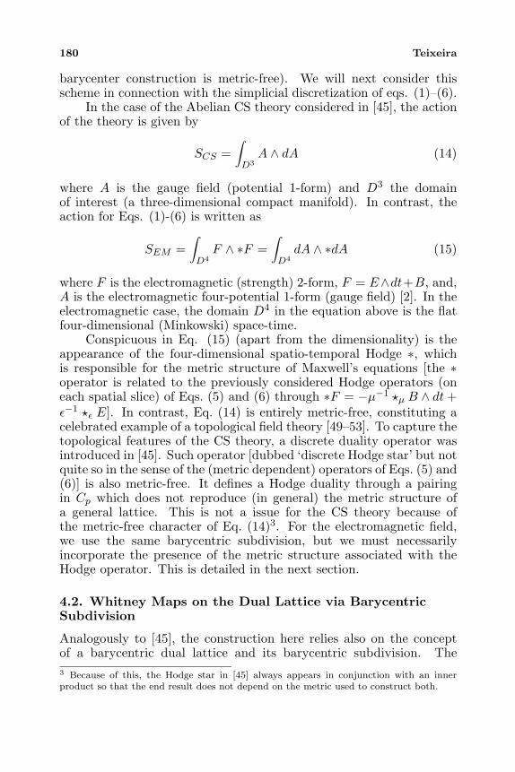
180 Teixeira
barycenter construction is metric-free). We will next consider thisscheme in connection with the simplicial discretization of eqs. (1)–(6).
In the case of the Abelian CS theory considered in [45], the actionof the theory is given by
SCS =∫D3
A ∧ dA (14)
where A is the gauge field (potential 1-form) and D3 the domainof interest (a three-dimensional compact manifold). In contrast, theaction for Eqs. (1)-(6) is written as
SEM =∫D4
F ∧ ∗F =∫D4
dA ∧ ∗dA (15)
where F is the electromagnetic (strength) 2-form, F = E∧dt+B, and,A is the electromagnetic four-potential 1-form (gauge field) [2]. In theelectromagnetic case, the domain D4 in the equation above is the flatfour-dimensional (Minkowski) space-time.
Conspicuous in Eq. (15) (apart from the dimensionality) is theappearance of the four-dimensional spatio-temporal Hodge ∗, whichis responsible for the metric structure of Maxwell’s equations [the ∗operator is related to the previously considered Hodge operators (oneach spatial slice) of Eqs. (5) and (6) through ∗F = −µ−1 µ B ∧ dt+ε−1 ε E]. In contrast, Eq. (14) is entirely metric-free, constituting acelebrated example of a topological field theory [49–53]. To capture thetopological features of the CS theory, a discrete duality operator wasintroduced in [45]. Such operator [dubbed ‘discrete Hodge star’ but notquite so in the sense of the (metric dependent) operators of Eqs. (5) and(6)] is also metric-free. It defines a Hodge duality through a pairingin Cp which does not reproduce (in general) the metric structure ofa general lattice. This is not a issue for the CS theory because ofthe metric-free character of Eq. (14)3. For the electromagnetic field,we use the same barycentric subdivision, but we must necessarilyincorporate the presence of the metric structure associated with theHodge operator. This is detailed in the next section.
4.2. Whitney Maps on the Dual Lattice via BarycentricSubdivision
Analogously to [45], the construction here relies also on the conceptof a barycentric dual lattice and its barycentric subdivision. The3 Because of this, the Hodge star in [45] always appears in conjunction with an innerproduct so that the end result does not depend on the metric used to construct both.
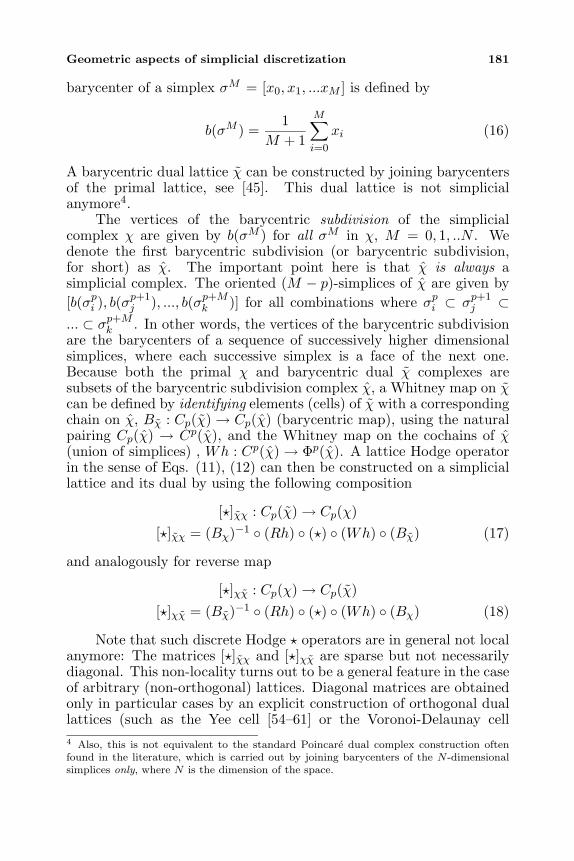
Geometric aspects of simplicial discretization 181
barycenter of a simplex σM = [x0, x1, ...xM ] is defined by
b(σM ) =1
M + 1
M∑i=0
xi (16)
A barycentric dual lattice χ can be constructed by joining barycentersof the primal lattice, see [45]. This dual lattice is not simplicialanymore4.
The vertices of the barycentric subdivision of the simplicialcomplex χ are given by b(σM ) for all σM in χ, M = 0, 1, ..N . Wedenote the first barycentric subdivision (or barycentric subdivision,for short) as χ. The important point here is that χ is always asimplicial complex. The oriented (M − p)-simplices of χ are given by[b(σpi ), b(σ
p+1j ), ..., b(σp+Mk )] for all combinations where σpi ⊂ σp+1
j ⊂... ⊂ σp+Mk . In other words, the vertices of the barycentric subdivisionare the barycenters of a sequence of successively higher dimensionalsimplices, where each successive simplex is a face of the next one.Because both the primal χ and barycentric dual χ complexes aresubsets of the barycentric subdivision complex χ, a Whitney map on χcan be defined by identifying elements (cells) of χ with a correspondingchain on χ, Bχ : Cp(χ)→ Cp(χ) (barycentric map), using the naturalpairing Cp(χ) → Cp(χ), and the Whitney map on the cochains of χ(union of simplices) , Wh : Cp(χ)→ Φp(χ). A lattice Hodge operatorin the sense of Eqs. (11), (12) can then be constructed on a simpliciallattice and its dual by using the following composition
[]χχ : Cp(χ)→ Cp(χ)[]χχ = (Bχ)−1 (Rh) () (Wh) (Bχ) (17)
and analogously for reverse map
[]χχ : Cp(χ)→ Cp(χ)[]χχ = (Bχ)−1 (Rh) () (Wh) (Bχ) (18)
Note that such discrete Hodge operators are in general not localanymore: The matrices []χχ and []χχ are sparse but not necessarilydiagonal. This non-locality turns out to be a general feature in the caseof arbitrary (non-orthogonal) lattices. Diagonal matrices are obtainedonly in particular cases by an explicit construction of orthogonal duallattices (such as the Yee cell [54–61] or the Voronoi-Delaunay cell4 Also, this is not equivalent to the standard Poincare dual complex construction oftenfound in the literature, which is carried out by joining barycenters of the N -dimensionalsimplices only, where N is the dimension of the space.
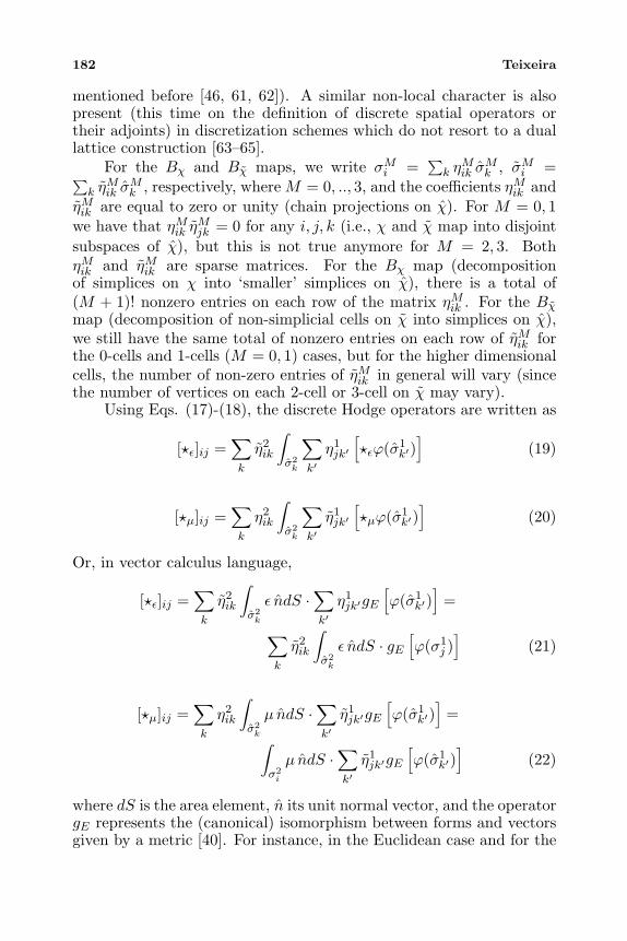
182 Teixeira
mentioned before [46, 61, 62]). A similar non-local character is alsopresent (this time on the definition of discrete spatial operators ortheir adjoints) in discretization schemes which do not resort to a duallattice construction [63–65].
For the Bχ and Bχ maps, we write σMi =∑k η
Mik σ
Mk , σMi =∑
k ηMik σ
Mk , respectively, where M = 0, .., 3, and the coefficients ηMik and
ηMik are equal to zero or unity (chain projections on χ). For M = 0, 1we have that ηMik η
Mjk = 0 for any i, j, k (i.e., χ and χ map into disjoint
subspaces of χ), but this is not true anymore for M = 2, 3. BothηMik and ηMik are sparse matrices. For the Bχ map (decompositionof simplices on χ into ‘smaller’ simplices on χ), there is a total of(M + 1)! nonzero entries on each row of the matrix ηMik . For the Bχmap (decomposition of non-simplicial cells on χ into simplices on χ),we still have the same total of nonzero entries on each row of ηMik forthe 0-cells and 1-cells (M = 0, 1) cases, but for the higher dimensionalcells, the number of non-zero entries of ηMik in general will vary (sincethe number of vertices on each 2-cell or 3-cell on χ may vary).
Using Eqs. (17)-(18), the discrete Hodge operators are written as
[ε]ij =∑k
η2ik
∫σ2k
∑k′η1jk′
[εϕ(σ1
k′)]
(19)
[µ]ij =∑k
η2ik
∫σ2k
∑k′η1jk′
[µϕ(σ1
k′)]
(20)
Or, in vector calculus language,
[ε]ij =∑k
η2ik
∫σ2k
ε ndS ·∑k′η1jk′gE
[ϕ(σ1
k′)]
=
∑k
η2ik
∫σ2k
ε ndS · gE[ϕ(σ1
j )]
(21)
[µ]ij =∑k
η2ik
∫σ2k
µ ndS ·∑k′η1jk′gE
[ϕ(σ1
k′)]
=
∫σ2i
µ ndS ·∑k′η1jk′gE
[ϕ(σ1
k′)]
(22)
where dS is the area element, n its unit normal vector, and the operatorgE represents the (canonical) isomorphism between forms and vectorsgiven by a metric [40]. For instance, in the Euclidean case and for the
Geometric aspects of simplicial discretization 183
1-forms (M = 1) in Eqs. (21)–(22), gE replaces the exterior derivatived in Eq. (13) by the nabla operator ∇ (this, together with the innerproduct with the area element dS, represents the metric in the vectorcalculus picture). The (arbitrary) choice of the ordinary complex (Eand B) as the primal (simplicial) and the twisted complex (D and H)as the dual (non-simplicial) is evident from the above equations.
The expressions on the right of Eqs. (21)–(22) (containing a singlesummation) result from the fact that the primal lattice χ is alreadysimplicial. However, these shortened expressions involve two spaces (χand χ) instead of a single one χ, and lack the symmetry of the middleexpressions with double summation which fully utilize the barycentricsubdivision and where the simplicial primal lattice does not play anyspecial role. Furthermore, they allow the elimination of any referenceto χ and χ, once the coefficients ηMik and ηMik are fixed, as also evidentin Eqs. (19)–(20).
Another property of the barycentric subdivision important tomention here and demonstrated in [47] is that, in conjunction withWhitney interpolations on the primal lattice, the chains of thebarycentric dual lattice are the assembling pieces of the surfaces forwhich flux conservation (2-forms) can be verified. This suggests a‘granular’ divergence-free condition at a discrete, interelement level.Recall that the divergence-free condition is not true in general forarbitrary surfaces because of the inter-element flux leaks (note alsothat this aspect involves both the primal and the dual latticessimultaneously, and therefore it does not follow from ∂2 = 0 on χor χ). This also indicates that such flux leaks are irrelevant if acertain granularity is assumed for the spatial domain according tothe barycentric subdivision. Integrations over domains which do notcomprise chains of the barycentric subdivision are in this sense justrendered meaningless.
5. CONCLUSIONS
Aspects of the discretization of Maxwell’s equations for generalsimplicial lattices using differential forms and algebraic topologicalconcepts have been discussed.
First, the treatment of the discrete counterpart to the topologicalpart of Maxwell’s equations was reviewed. This treatment employs theknown pairing between the dual spaces of cochains (discrete differentialforms) and chains (geometrical elements) on a cell complex.
Then, the role of the first barycentric subdivision to establishan isomorphism between the simplicial primal complex and the non-simplicial dual complex was stressed. A key property of the barycentric
184 Teixeira
dual complex and the barycentric subdivision complex is that they areboth metric-free constructions.
Under this rationale, we have shown that Whitney maps, definedon the first barycentric subdivision lattice, can be used to build discreteHodge operators (i.e., the discretization of the metric part of Maxwell’sequations encoded in the constitutive equations) for general simpliciallattices.
REFERENCES
1. Whitney, H., Geometric Integration Theory, Princeton UniversityPress, Princeton, 1957.
2. Misner, C. W., K. S. Thorne, and J. A. Wheeler, Gravitation,Freeman, New York, 1973.
3. Burke, W. L., Applied Differential Geometry, CambridgeUniversity Press, Cambridge, 1985.
4. Dodziuk, J., “Finite-difference approach to the Hodge theory ofharmonic forms,” Am. J. Math., Vol. 98, No. 1, 79–104, 1976.
5. Weingarten, D., “Geometric formulation of electrodynamics andgeneral relativity in discrete space-time,” J. Math. Phys., Vol. 18,No. 1, 165–170, 1977.
6. Muller, W., “Analytic torsion and R-torsion of Riemannianmanifolds,” Advances in Math., Vol. 28, 233–305, 1978.
7. Tonti, E., “On the mathematical strucuture of a large class ofphysical theories,” Rend. Acc. Lincei, Vol. 52, 48–56, 1972.
8. Tonti, E., “A mathematical model for physical theories,” Rend.Acc. Lincei, Vol. 52, 175–181, 1972.
9. Tonti, E., “The algebraic-topological structure of physicaltheories,” Proc. Conf. on Symmetry, Similarity, and GroupTheoretic Meth. in Mechanics, 441–467, Calgary, Canada, 1974.
10. Tonti, E., “On the geometrical structure of electromagnetism,”Gravitation, Electromagnetism, and Geometrical Structures, forthe 80th birthday of A. Lichnerowicz, G. Ferrarese (ed.), 281–308,Pitagora Editrice Bologna, 1995.
11. Tonti, E., “Algebraic topology and computational electromag-netism,” Proc. Fourth Int. Workshop on the Electric and MagneticFields: from Num. Meth. to Ind. Applicat., 284–294, Marseille,France, 1998.
12. Ohkuro, S., “Differential forms and Maxwell’s field: Anapplication of harmonic integrals,” J. Math. Phys., Vol. 11, No. 6,2005–2012, 1970.
Geometric aspects of simplicial discretization 185
13. Deschamps, G. A., “Electromagnetics and differential forms,”Proc. IEEE, Vol. 69, No. 6, 676–696, 1981.
14. Kheyfets, A. and W. A. Miller, “The boundary of a boundaryprinciple in field theories and the issue of austerity of the laws ofphysics,” J. Math. Phys., Vol. 32, No. 11, 3168–3175, 1991.
15. Bossavit, A., “Whitney forms: a new class of finite elements forthree-dimensional computations in electromagnetics,” IEE Proc.A, Vol. 135, 493–500, 1988.
16. Bossavit, A., “Simplicial finite elements for scattering problemsin electromagnetism,” Comp. Meth. Appl. Mech. Engineering,Vol. 76, 299–316, 1989.
17. Kotiuga, P. R., “Hodge decompositions and computationalelectromagnetics,” Ph.D. Thesis, Department of ElectricalEngineering, McGill University, Montreal, Canada, 1984.
18. Kotiuga, P. R., “Variational principles for three-dimensionalmagnetostatics based on helicity,” J. Appl. Phys., Vol. 63, No. 8,3360–3362, 1988.
19. Kotiuga, P. R., “Helicity functionals and metric invariance in threedimensions,” IEEE Trans. Magn., Vol. 25, No. 4, 2813–2815, 1989.
20. Kotiuga, P. R., “Analysis of finite-element matrices arising fromdiscretizations of helicity functionals,” J. Appl. Phys., Vol. 67,No. 9, 5815–5817, 1990.
21. Kotiuga, P. R., “Metric dependent aspects of inverse problemsand functionals based on helicity,” J. Appl. Phys., Vol. 73, No. 10,5437–5439, 1993.
22. Hammond, P. and D. Baldomir, “Dual energy methods inelectromagnetism using tubes and slices,” IEEE Proc. A, Vol. 135,No. 3, 167–172, 1988.
23. Bossavit, A., “Differential forms and the computation of fieldsand forces in electromagnetism,” Eur. J. Mech. B, Vol. 10, No. 5,474–488, 1991.
24. Bossavit, A., Computational Electromagnetism: VariationalFormulations, Complementarity, Edge Elements, Academic Press,New York, 1998.
25. Kettunen, L., K. Forsman, and A. Bossavit, “Discrete spaces forDiv and Curl-free fields,” IEEE Trans. Magn., Vol. 34, No. 5,2551–2554, 1998.
26. Tarhasaari, T., L. Kettunen, and A. Bossavit, “Some realizationsof a discrete Hodge operator: A reinterpretation of finite elementtechniques,” IEEE Trans. Magn., Vol. 35, No. 3, 1494–1497, 1999.
27. Bossavit, A., “A posteriori error bounds by ‘local corrections’
186 Teixeira
using the dual mesh,” IEEE Trans. Magn., Vol. 35, No. 3, 1350–1353, 1999.
28. Bossavit, A., “On the notion of anisotropy of constitutive laws:Some implications of the ‘Hodge implies metric’ result,” privatecommunication.
29. Becher, P. and H. Joos, “The Dirac-Kahler equation and fermionson the lattice,” Z. Phys. C, Vol. 15, 343–365, 1982.
30. Warnick, K. F., R. H. Selfridge, and D. V. Arnold, “Electromag-netic boundary conditions and differential forms,” IEE Proc., Mi-crow. Ant. Prop., Vol. 142, 326–332, 1995.
31. Jancewicz, B., “A variable metric electrodynamics. The Coulomband Biot-Savart laws in anisotropic media,” Ann. Phys., Vol. 245,227–274, 1996.
32. Mattiussi, C., “An analysis of finite volume, finite element, andfinite difference methods using some concepts from algebraictopology,” J. Comp. Phys., Vol. 133, 289–309, 1997.
33. Warnick, K. F., R. H. Selfridge, and D. V. Arnold, “Teachingeletromagnetic field theory using differential forms,” IEEE Trans.Edu., Vol. 40, No. 1, 53–68, 1997.
34. Warnick, K. F. and D. V. Arnold, “Green forms for anisotropic,inhomogeneous media,” J. Electromagn. Waves Appl., Vol. 11,No. 8, 1145–1164, 1997.
35. Arkko, A., T. Tarhasaari, and L. Kettunen, “A time domainmethod for high frequency problems exploring the Whitneycomplex,” Proc. 14th. Ann. Rev. Prog. Appl. Comp. Electromag.Soc., 121–126, Monterey, CA, 1998.
36. Kraus, C. and R. Ziolkowsky, “Topological and geometricalconsiderations for Maxwell’s equations on unstructured meshes,”Proc. URSI Meeting, 714, Montreal, Canada, 1997.
37. Hiptmair, R., “Canonical construction of finite elements,” Math.Computat., Vol. 68,, 1325–1346, 1999.
38. Hiptmair, R., “Discrete Hodge operators,” Tech. Rep. 126, SFB382, University of Tubingen, Tubingen, Germany, 1999.
39. Teixeira, F. L. and W. C. Chew, “Differential forms, metrics,and the reflectionless absorption of electromagnetic waves,” J.Electromagn. Waves Applicat., Vol. 13, No. 5, 665–686, 1999.
40. Teixeira, F. L. and W. C. Chew, “Lattice electromagnetic theoryfrom a topological viewpoint,” J. Math. Phys., Vol. 40, No. 1,169–187, 1999.
41. Albeverio, S. and B. Zegarlinski, “Construction of convergentsimplicial approximations of quantum field on Riemannian
Geometric aspects of simplicial discretization 187
manifolds,” Comm. Math. Phys., Vol. 132, 39–71, 1990.42. Albeverio, S. and J. Schafer, “Abelian Chern-Simons theory and
linking numbers via oscilatory integrals,” J. Mat. Phys., Vol. 36,No. 5, 2157–2169, 1995.
43. Adams, D. H., “R-torsion and linking numbers from simplicialAbelian gauge theories,” eprint http://arxiv.org/archive/hep-th/961209, 1996.
44. Adams, D. H., “A double discretization of Abelian Chern-Simonstheory,” Phys. Rev. Lett., Vol. 78, No. 22, 4155–4158, 1997.
45. Sen, S., S. Sen, J. C. Sexton, and D. H. Adams, “Geometricdiscretization scheme applied to the Abelian Chern-Simonstheory,” Phys. Rev. E, Vol. 61, No. 3, 3174–3185, 2000.
46. Kojima, T., Y. Saito, and R. Dang. “Dual mesh approach forsemiconductor device simulator,” IEEE Trans. Magn., Vol. 25,No. 4, 2953–2955, 1989.
47. Bossavit, A., “How weak is the ‘weak solution’ in finite elementmethods,” IEEE Trans. Magn., Vol. 34, No. 5, 2429–2432, 1998.
48. Bossavit, A. and L. Kettunen, “Yee-schemes on a tetrahedralmesh, with diagonal lumping,” Int. J. Num. Model., Vol. 12, 129–142, 1999.
49. Witten, E., “Topological quantum field theory,” Comm. Math.Phys., Vol. 117, 353–386, 1988.
50. Fukuma, M., S. Hosono, and H. Kawai, “Lattice topological fieldtheory in two dimensions,” Comm. Math. Phys., Vol. 161, 157–175, 1994.
51. Chung, S.-W., M. Fukuma, and A. Shapere, “Structure oftopological lattice field theory in three dimensions,” Int. J. Mod.Phys., Vol. 9, No. 8, 1305–1360, 1994.
52. da Cunha, B. G. C. and P. T. Sobrinho, “Quasitopological fieldtheories in two dimensions as soluble models,” Int. J. Mod. Phys.,Vol. 13, No. 21, 3667–3689, 1998.
53. Felder, G., J, Frolich, J. Fuchs, and C. Schweigert, “Conformalboundary conditions and three-dimensional topological fieldtheory,” Phys. Rev. Lett., Vol. 84, No. 8, 1659–1662, 2000.
54. Yee, K. S., “Numerical solution of initial boundary value problemsinvolving Maxwell’s equations in isotropic media,” IEEE Trans.Ant. Propagat., Vol. 14, 302–307, 1966.
55. Taflove, A., Computational Electrodynamics: The Finite-Difference Time-Domain Method, Artech House, Boston, 1995.
56. Weiland, T., “On the numerical solutions of Maxwell’s equationsand applications in the field of accelerator physics,” Particle
188 Teixeira
Accelerators, Vol. 15, 245–292, 1984.57. Weiland, T., “Time domain electromagnetic field computations
with finite difference methods,” Int. J. Num. Model., Vol. 9, 295–319, 1996.
58. Chew, W. C., “Electromagnetic theory on a lattice,” J. Appl.Phys., Vol. 75, No. 10, 4843–4850, 1994.
59. Radhakrishnan, K. and W. C. Chew, “Full-wave analysis ofmulticonductor transmission lines on anisotropic inhomogeneoussubstrates,” IEEE Trans. Microwave Theory Tech., Vol. 47, No. 9,1764–1771, 1999.
60. Mattiussi, C., “Finite volume, finite difference, and finiteelement methods for physical field problems,” Advancing ImagingElectron. Phys., Vol. 113, 1–146, 2000.
61. McCartin, B. J. and J. F. DiCello, “Three dimensional finitedifference frequency domain scattering computation using thecontrol region approximation,” IEEE Trans. Magn., Vol. 25,No. 4, 3092–3094, 1989.
62. Rappaport, C. M. and E. B. Smith, “Anisotropic FDFD computedon conformal meshes,” IEEE Trans. Magn., Vol. 27, No. 5, 3848–3851, 1991.
63. Hyman, J. M. and M. Shashkov, “Natural discretization forthe divergence, gradient and curl on logically rectangular grids,”Comput. Math. Appl., Vol. 33, 81–104, 1997.
64. Hyman, J. M. and M. Shashkov, “Adjoint operators for thenatural discretization for the divergence, gradient and curl onlogically rectangular grids,” Appl. Num. Math., Vol. 25, 413–442,1997.
65. Hyman, J. M. and M. Shashkov, “Mimetic discretizations forMaxwell’s equations,” J. Comp. Phys., Vol. 151, 881–909, 1999.
Progress In Electromagnetics Research, PIER 32, 189–206, 2001
TOPOLOGICAL APPROACH TO COMPUTATIONALELECTROMAGNETISM
T. Tarhasaari and L. Kettunen
Laboratory of ElectromagneticsTampere University of TechnologyP.O. Box 692, FIN-33101 Tampere, Finland
Abstract—Software systems designed to solve Maxwell’s equationsneed abstractions that accurately explain what different kinds ofelectromagnetic problems really do have in common. Computationalelectromagnetics calls for higher level abstractions than what istypically needed in ordinary engineering problems. In this paperMaxwell’s equations are described by exploiting basic concepts ofset theory. Although our approach unavoidably increases the levelof abstraction, it also simplifies the overall view making it easier torecognize a topological problem behind all boundary value problemsmodeling the electromagnetic phenomena. This enables us also toconstruct an algorithm which tackles the topological problem withbasic tools of linear algebra.
1 Introduction
2 Maxwell Equations as Relations
3 Topological Problem
4 Exact Sequences and Decompositions
5 Bounded Domains
6 Implementation6.1 Algorithm6.2 Example6.3 Practical Issues
Acknowledgment
References
190 Tarhasaari and Kettunen
1. INTRODUCTION
Electromagnetic phenomena is fully described by the Maxwellequations, which are typically described in terms of vector algebra.Although seldom mentioned, in the background such an approachrelies on an Euclidean space, which is what enables one to talk ofdistances and angles, or of magnitudes of vectors. Since the notionsof distances and angles are everyday routines, one may arrive at aconclusion that physics (i.e., modeling of nature) somehow did requireEuclidean spaces. But to recognize the nature of Euclidean spaces,let us call them with another name: “Euclidean” is a synonym to pre-Hilbertian with finitude of dimension usually implied. Here, there is noneed to go to the details of pre-Hilbertian spaces [1], it is just enoughto realize that they are something which are made of several layers ofstructures: An Euclidean space is not a simple structure.
As is argued in [2] science is about trying to understand and seewhat complicated and diverse events really do have in common and toexplain or to describe the behaviour accurately, simply and elegantly.When it comes to electromagnetism, vector fields and Euclidean spacesare a heavier structure than needed [3, 4, 5, 6], and they may blockfrom seeing the principal information of Maxwell’s equations. Theirony is that Euclidean spaces and vector fields are rather intuitive.As soon as simpler –and thus, in principle, easier– structures areemployed, unavoidably the level of abstraction has to increase. Thisis perhaps why the more powerful, accurate, and elegant models areeasily considered less physical. Some may even questioned whetherthey are needed at all.
The nature of software design is very close to that of science.The fundamental problem in developing software is to find the right,i.e., simple, accurate, and elegant abstractions [7]. Computationalelectromagnetism makes no difference, and thus, there is a practicalcall to find better abstractions describing Maxwell’s equations in aprecise and elegant way, and such that they become easily convertibleinto pieces of software.
The software systems developed for electromagnetic design aretypically inflexible requiring the user to input certain data (sometimeseven in a certain order) to generate the result the user needs.Furthermore, such systems may also suffer for the problem that theyare not able to recognize missing, incorrect, or conflicting data until itgets to the point when the solution process of a system of equationsfails. But even then, there are little tools to recognize what really wentwrong. One reason for this inflexibility is perhaps the method drivenapproach commonly employed in generating software. In other words,
Topological approach to CEM 191
the software is a realization of some methods and algorithms, and theuser is required to insert data which fits into this model. Of course,the software may try to list out all cases that are not solvable, but thisis an extensive and unreliable approach.
The motivation for this paper comes from the opposite direction.The idea is to develop a data driven approach which by an abstractrepresentation of the category of problems generates by top-downdevelopment an orderly (code) structure, which then enables torecognize what can or cannot be done with the data inserted by theuser. The very idea is that the software system is driven by the inserteddata instead of trying to fit data into a priori selected approach.
It is plain that in a single paper there is not enough roomto thoroughly discuss such a topic. (There are books, such as[8], published in this kind of questions). In this paper we shallfocus on the topological issues behind Maxwell’s equations. In thefirst part of the paper we introduce a topological problem behindelectromagnetic problems. By employing the language of differentialgeometry [9, 10, 11, 12, 3, 4, 5, 6] and algebraic topology [13], andespecially of homology [13, 14, 15], we shall express Maxwell’s equationsusing some simple concepts of set theory. In the second part weintroduce an algorithm exploiting the basic tools of linear algebra totackle the topological problem introduced in the first part. In addition,an example and some practical hints are presented.
2. MAXWELL EQUATIONS AS RELATIONS
Electromagnetic fields are characterized by Maxwell’s equations. Theirmain information is in how the integral of a field over the boundaryof any chain [16] matches with the integral of some other field overthat chain. In more formal terms, the boundary operator ∂p is a mapfrom the module Cp of all p-chains into the module Cp−1 containingall (p − 1)-chains. Thus, a chain and its boundary are linked by (thegraph of) a relation R(∂p) ⊂ Cp × Cp−1, and evidently for all pairs(c, c′) ∈ R(∂p) one has
(c, c′) ∈ R(∂p) ⇔ ∂pc = c′ .
Maxwell’s equations involve integration, which is a bilinearoperator from the cartesian product of Cp and the space F p of p-cochains to the field of reals R (or to some other field F):
∫ p
: Cp × F p → R .
192 Tarhasaari and Kettunen
In general, if one has bilinear operators f1 : A1 × B1 → F andf2 : A2 × B2 → F, and R(A) is a linear relation in (i.e., a linearsubspace of) the cartesian product A1 × A2, then relation R(A) andoperators f1, f2 induce a linear relation R(A, f) ⊂ B1 × B2 suchthat (b1, b2) ∈ R(A, f) if and only if for all (a1, a2) ∈ R(A) holdf1(a1, b1) = f2(a2, b2).
Relation R(∂p) is linear –i.e., the boundary operator is linear– andthus, R(∂p) and the integral operators
∫ p
: Cp × F p → R
∫ p−1
: Cp−1 × F p−1 → R,
induce relation R(∂p,∫ p) ⊂ F p×F p−1 such that, if (f, g) ∈ R(∂p,
∫ p)then ∫
c
p
f =∫c′
p−1
g
has to hold for all (c, c′) ∈ R(∂p).Maxwell’s equations may be considered as this kind of induced
relations. For instance, Ampere’s law∫∂c
h =∫c
(j + ∂td) , (1)
expressing the relationship between magnetic field h and current j andthe time derivative of electric flux d can be interpreted as a relation(j + ∂td, h) ∈ R(∂2,
∫ 2). Correspondingly, Gauss’s law∫∂c
b =∫c
qm (2)
saying the magnetic flux b over all bounding 2-chains should equal tothe magnetic charge qm that chain bounds can be viewed as a relation(qm, b) ∈ R(∂3,
∫ 3).A relation R(A) ⊂ A1 × A2 is said to be one-to-one if there
is a 1-to-1 correspondence between the elements a1 and a2 of pair(a1, a2) ∈ R(A). The constitutive laws can also be interpreted asrelations. We assume that permeability µ belongs to the set Mof “admissible” permeabilities, and that n is the dimension of the
Topological approach to CEM 193
ambient space. Then, the constitutive law corresponds with a one-to-one relation R1−1(µ) ∈ F 2×F 1 defined with aid of the Hodge operator∗ mapping p-cochains into (n− p)-cochains [10] such that
(b, h) = R1−1(µ) ⇔ b = µ ∗h .
Besides the emphasis shifted towards the principal information ofMaxwell’s equations, the motivation for the use of relations is that suchnotions of naive set theory [17] can easily be transformed into piecesof software.
3. TOPOLOGICAL PROBLEM
The tools we have enable us to formulate electromagnetic problems inan alternative way. Let us assume that µ ∈ M , i = j + ∂td ∈ F 2,and qm ∈ F 3 are known in all space. Then the magnetic field is thesolution of problem:Problem 1: Find (b, h) ∈ F 2 × F 1 such that
(b, h) ∈ R1−1(µ) ,
(j + ∂td, h) ∈ R(∂2,∫ 2) ,
(qm, b) ∈ R(∂3,∫ 3)
hold.Problem 1 is not, however, well posed. The conditions for the
solution are sufficient in the sense that if there is a solution, then thesolution is also unique. But the existence of the solution depends onwhether i is solenoidal1 or not.
In practical software design such problems are typically avoidedby testing whether the inserted data fits into the model. However,since our goal was to develop a data driven approach to computationalelectromagnetism, we shall tackle the problem in another way.
To go on, we need next to introduce the concept of an isomorphicrelation. A relation is isomorphic if it is one-to-one and linear. Letus now denote by cod(∂p) the codomain (range) of operator ∂p. If thelinear relation R(∂p) ⊂ Cp × Cp−1 is restricted such that the map
∂p : C ′p → cod(∂p)
is an isomorphism from C ′p onto cod(∂p), then the relation R(∂p) ⊂C ′p × cod(∂p) in the restricted space is obviously also isomorphic.
1 A field f ∈ F 2 is solenoidal if its integral over all bounding 2-chains (of the form c = ∂3c′)vanish.
194 Tarhasaari and Kettunen
When the relation R(∂p) is isomorphic, symbol Ri(∂p) is employedto emphasize this property.
The key point is that existence of the solution of problem 1can be guaranteed if relations R(∂2, ∫2) and R(∂3, ∫3) are induced byisomorphic relations Ri(∂2) and Ri(∂3). In such cases we shall usesymbols Ri(∂2, ∫2) and Ri(∂3, ∫3) to denote this property.
Now, the topological problem of “conflicting” data is resolved.With the same assumptions as above the magnetic field can becharacterized as the solution of problem:Problem 2: Find (b, h) ∈ F 2 × F 1 such that
(b, h) ∈ R1−1(µ) ,
(j + ∂td, h) ∈ Ri(∂2,∫ 2) ,
(qm, b) ∈ Ri(∂3,∫ 3)
hold. This is a well posed problem meaning there exists a uniquesolution2 for it.
When it comes to numerical computation there still remains analgebraic problem of finding a linearly independent basis for Ri(∂2)and Ri(∂3). In practice this means that Ampere’s and Gauss’s lawsneed not to be imposed over all pairs (c, ∂c) in Ri(∂2) and Ri(∂3), butinstead only over sets which form linearly independent bases of theserelations.
Obviously, the electric field makes no difference with respect tothe magnetic field, so as an immediate generalization we may state:In computational electromagnetics there is a problem of algebraictopology to find isomorphic relations Ri(∂p) and a problem of linearalgebra constructing linearly independent bases for these spaces.
4. EXACT SEQUENCES AND DECOMPOSITIONS
The isomorphic relation Ri(∂p) is related to so called exact sequences,which are sequences of abelian groups in the following way: A mappingα from abelian group U to another abelian group V is a homomorphismpreserving the structure if α satisfies α(ai + aj) = α(ai) + α(aj). Asequence of abelian groups and homomorphisms
· · · −→ Un+1αn+1−→ Un
αn−→ Un−1 −→ . . .
2 All the solutions of problem 1 are also solutions of problem 2, but not vice versa.Furthermore, if the first problem has a solution, it is also a solution of the second one.
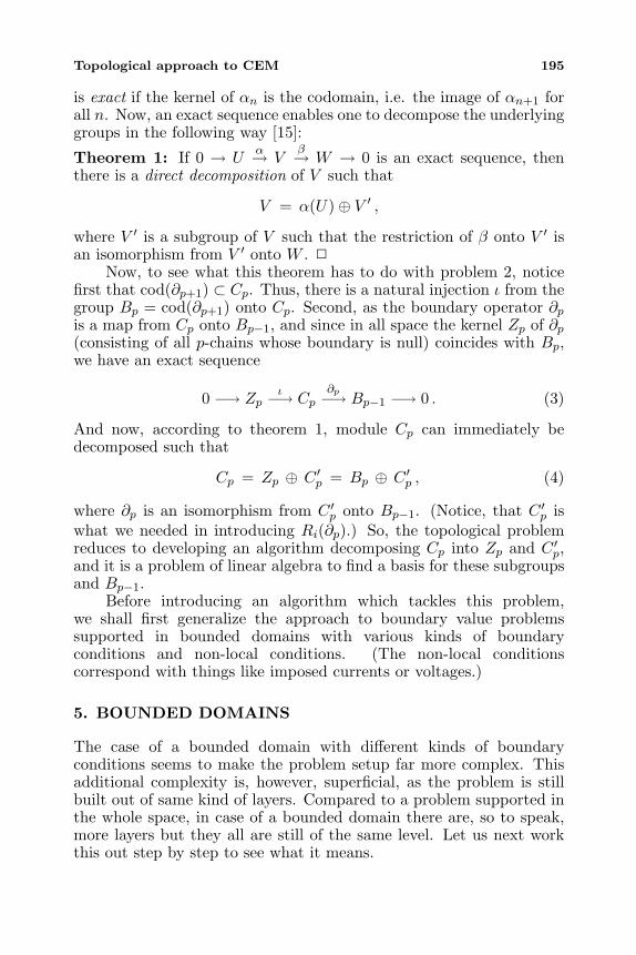
Topological approach to CEM 195
is exact if the kernel of αn is the codomain, i.e. the image of αn+1 forall n. Now, an exact sequence enables one to decompose the underlyinggroups in the following way [15]:
Theorem 1: If 0 → Uα→ V
β→ W → 0 is an exact sequence, thenthere is a direct decomposition of V such that
V = α(U)⊕ V ′ ,
where V ′ is a subgroup of V such that the restriction of β onto V ′ isan isomorphism from V ′ onto W .
Now, to see what this theorem has to do with problem 2, noticefirst that cod(∂p+1) ⊂ Cp. Thus, there is a natural injection ι from thegroup Bp = cod(∂p+1) onto Cp. Second, as the boundary operator ∂pis a map from Cp onto Bp−1, and since in all space the kernel Zp of ∂p(consisting of all p-chains whose boundary is null) coincides with Bp,we have an exact sequence
0 −→ Zpι−→ Cp
∂p−→ Bp−1 −→ 0 . (3)
And now, according to theorem 1, module Cp can immediately bedecomposed such that
Cp = Zp ⊕ C ′p = Bp ⊕ C ′p , (4)
where ∂p is an isomorphism from C ′p onto Bp−1. (Notice, that C ′p iswhat we needed in introducing Ri(∂p).) So, the topological problemreduces to developing an algorithm decomposing Cp into Zp and C ′p,and it is a problem of linear algebra to find a basis for these subgroupsand Bp−1.
Before introducing an algorithm which tackles this problem,we shall first generalize the approach to boundary value problemssupported in bounded domains with various kinds of boundaryconditions and non-local conditions. (The non-local conditionscorrespond with things like imposed currents or voltages.)
5. BOUNDED DOMAINS
The case of a bounded domain with different kinds of boundaryconditions seems to make the problem setup far more complex. Thisadditional complexity is, however, superficial, as the problem is stillbuilt out of same kind of layers. Compared to a problem supported inthe whole space, in case of a bounded domain there are, so to speak,more layers but they all are still of the same level. Let us next workthis out step by step to see what it means.
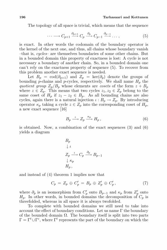
196 Tarhasaari and Kettunen
The topology of all space is trivial, which means that the sequence
· · · −→ Cp+1∂p+1−→ Cp
∂p−→ Cp−1∂p−1−→ . . . , (5)
is exact. In other words the codomain of the boundary operator isthe kernel of the next one, and thus, all chains whose boundary vanish–that is, cycles– are themselves boundaries of some other chains. Butin a bounded domain this property of exactness is lost: A cycle is notnecessary a boundary of another chain. So, in a bounded domain onecan’t rely on the exactness property of sequence (5). To recover fromthis problem another exact sequence is needed.
Let Bp = cod(∂p+1) and Zp = ker(∂p) denote the groups ofbounding p-chains and p-cycles, respectively. We shall name Hp thequotient group Zp/Bp whose elements are cosets of the form z + Bp
where z ∈ Zp. This means that two cycles z1, z2 ∈ Zp belong to thesame coset of Hp if z1 − z2 ∈ Bp. As all bounding chains are alsocycles, again there is a natural injection ι : Bp → Zp. By introducingoperator κp taking a cycle z ∈ Zp into the corresponding coset of Hp,a new exact sequence [16]
Bpι−→ Zp
κp−→ Hp , (6)
is obtained. Now, a combination of the exact sequences (3) and (6)yields a diagram
Bp
↓ ι
Zpι−→ Cp
∂p−→ Bp−1
↓ κpHp ,
and instead of (4) theorem 1 implies now that
Cp = Zp ⊕ C ′p = Bp ⊕ Z ′p ⊕ C ′p , (7)
where ∂p is an isomorphism from C ′p onto Bp−1 and κp from Z ′p ontoHp. In other words, in bounded domains the decomposition of Cp isthreefolded, whereas in all space it is always twofolded.
To complete with bounded domains we still need to take intoaccount the effect of boundary conditions. Let us name Γ the boundaryof the bounded domain Ω. The boundary itself is split into two partsΓ = Γt∪Γc, where Γt represents the part of the boundary on which the
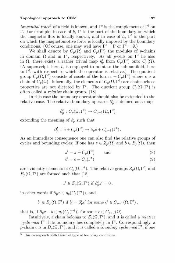
Topological approach to CEM 197
tangential trace3 of a field is known, and Γc is the complement of Γt onΓ. For example, in case of b, Γt is the part of the boundary on whichthe magnetic flux is locally known, and in case of h, Γt is the parton which the magnetomotive force is locally imposed by the boundaryconditions. (Of course, one may well have Γt = Γ or Γt = ∅.)
We shall denote by Cp(Ω) and Cp(Γt) the modules of p-chainsin domain Ω and in Γt, respectively. As all p-cells on Γt lie alsoin Ω, there exists a rather trivial map ηtp from Cp(Γt) onto Cp(Ω).(A superscript, here t, is employed to point to the submanifold, hereto Γt, with respect to which the operator is relative.) The quotientgroup Cp(Ω,Γt) consists of cosets of the form c + Cp(Γt) where c is achain of Cp(Ω). Informally, the elements of Cp(Ω,Γt) are chains whoseproperties are not dictated by Γt. The quotient group Cp(Ω,Γt) isoften called a relative chain group. [18]
In this case the boundary operator should also be extended to therelative case. The relative boundary operator ∂tp is defined as a map
∂tp : Cp(Ω,Γt)→ Cp−1(Ω,Γt)
extending the meaning of ∂p such that
∂tp : c + Cp(Γt)→ ∂pc + Cp−1(Γt) .
As an immediate consequence one can also find the relative groups ofcycles and bounding cycles: If one has z ∈ Zp(Ω) and b ∈ Bp(Ω), then
z′ = z + Cp(Γt) and (8)
b′ = b + Cp(Γt) (9)
are evidently elements of Cp(Ω,Γt). The relative groups Zp(Ω,Γt) andBp(Ω,Γt) are formed such that [18]
z′ ∈ Zp(Ω,Γt) if ∂tpz′ = 0 ,
in other words if ∂pz ∈ ηp(Cp(Γt)), and
b′ ∈ Bp(Ω,Γt) if b′ = ∂tpc′ for some c′ ∈ Cp+1(Ω,Γt) ,
that is, if ∂pc− b ∈ ηp(Cp(Γt)) for some c ∈ Cp+1(Ω).Intuitively, a chain belongs to Zp(Ω,Γt), and it is called a relative
cycle mod Γt if its boundary lies completely in Γt. Correspondingly, ap-chain c is in Bp(Ω,Γt), and it is called a bounding cycle mod Γt, if one3 This corresponds with Dirichlet type of boundary conditions.
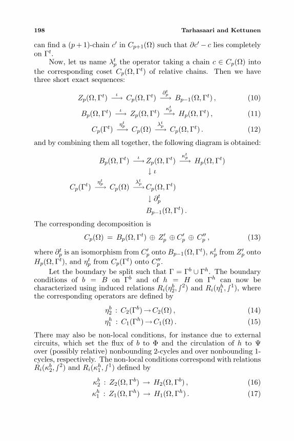
198 Tarhasaari and Kettunen
can find a (p+ 1)-chain c′ in Cp+1(Ω) such that ∂c′− c lies completelyon Γt.
Now, let us name λtp the operator taking a chain c ∈ Cp(Ω) intothe corresponding coset Cp(Ω,Γt) of relative chains. Then we havethree short exact sequences:
Zp(Ω,Γt) ι−→ Cp(Ω,Γt)∂tp−→ Bp−1(Ω,Γt) , (10)
Bp(Ω,Γt) ι−→ Zp(Ω,Γt)κtp−→ Hp(Ω,Γt) , (11)
Cp(Γt)ηtp−→ Cp(Ω)
λtp−→ Cp(Ω,Γt) . (12)
and by combining them all together, the following diagram is obtained:
Bp(Ω,Γt) ι−→Zp(Ω,Γt)κtp−→ Hp(Ω,Γt)
↓ ι
Cp(Γt)ηtp−→ Cp(Ω)
λtp−→Cp(Ω,Γt)
↓ ∂tpBp−1(Ω,Γt) .
The corresponding decomposition is
Cp(Ω) = Bp(Ω,Γt) ⊕ Z ′p ⊕ C ′p ⊕ C ′′p , (13)
where ∂tp is an isomorphism from C ′p onto Bp−1(Ω,Γt), κtp from Z ′p ontoHp(Ω,Γt), and ηtp from Cp(Γt) onto C ′′p .
Let the boundary be split such that Γ = Γb ∪ Γh. The boundaryconditions of b = B on Γb and of h = H on Γh can now becharacterized using induced relations Ri(ηb2, ∫2) and Ri(ηh1 , ∫1), wherethe corresponding operators are defined by
ηb2 : C2(Γb)→C2(Ω) , (14)
ηh1 : C1(Γh)→C1(Ω) . (15)
There may also be non-local conditions, for instance due to externalcircuits, which set the flux of b to Φ and the circulation of h to Ψover (possibly relative) nonbounding 2-cycles and over nonbounding 1-cycles, respectively. The non-local conditions correspond with relationsRi(κb2, ∫2) and Ri(κh1 , ∫1) defined by
κb2 : Z2(Ω,Γb) → H2(Ω,Γb) , (16)
κh1 : Z1(Ω,Γh) → H1(Ω,Γh) . (17)
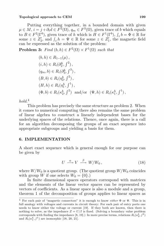
Topological approach to CEM 199
Putting everything together, in a bounded domain with givenµ ∈M , i = j+∂td ∈ F 2(Ω), qm ∈ F 3(Ω), given trace of b which equalsto B ∈ F 2(Γb), given trace of h which is H ∈ F 1(Γb), ∫z b = Φ ∈ R forsome z ∈ Z ′2, and ∫z h = Ψ ∈ R for some z ∈ Z ′1, the magnetic fieldcan be expressed as the solution of the problem:Problem 3: Find (b, h) ∈ F 2(Ω)× F 1(Ω) such that
(b, h) ∈ R1−1(µ) ,
(i, h) ∈ Ri(∂h2 ,∫ 2) ,
(qm, b) ∈ Ri(∂b3,∫ 3) ,
(B, b) ∈ Ri(ηb2,∫ 2) ,
(H,h) ∈ Ri(ηh1 ,∫ 1) ,
(Φ, b) ∈ Ri(κb2,∫ 2) and/or (Ψ, h) ∈ Ri(κh1 ,
∫ 1) ,
hold.4This problem has precisely the same structure as problem 2. When
it comes to numerical computing there also remains the same problemof linear algebra to construct a linearly independent bases for theunderlying spaces of the relations. Thence, once again, there is a callfor an algorithm decomposing the groups of an exact sequence intoappropriate subgroups and yielding a basis for them.
6. IMPLEMENTATION
A short exact sequence which is general enough for our purpose canbe given by
Uα−→ V
β−→ W/W0 , (18)
where W/W0 is a quotient group. (The quotient group W/W0 coincideswith group W if one selects W0 = 0.)
In finite dimensional spaces operators correspond with matricesand the elements of the linear vector spaces can be represented byvectors of coefficients. As a linear space is also a module and a group,theorem 1 of the decomposition of groups applies to linear spaces as4 For each pair of “magnetic connectors” it is enough to know either Φ or Ψ. This is infull analogy with voltages and currents in circuit theory: For each pair of entry ports oneneeds to know either the voltage or current [19]. If they both are known, then there isnothing to solve, as the impedance Z = U/I is fixed. (Solving a boundary value problemcorresponds with finding the impedance [8, 19].) In more precise terms, relations Ri(κ
b2, ∫2)
and Ri(κh1 , ∫1) are isomorphic [18, 20, 21].
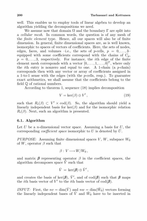
200 Tarhasaari and Kettunen
well. This enables us to employ tools of linear algebra to develop analgorithm yielding the decompositions we need.
We assume now that domain Ω and the boundary Γ are split intoa cellular mesh. In common words, the question is of any mesh ofthe finite element type. Hence, all our spaces will also be of finitedimension. In general, finite dimensional spaces are, as is well known,isomorphic to spaces of vectors of coefficients. Here, the sets of nodes,edges, faces, and volumes –i.e., the sets of p-cells, p = 0, . . . , 3–equipped with some coefficients correspond with the chains of Cp,p = 0, . . . , 3, respectively. For instance, the ith edge of the finiteelement mesh corresponds with a vector [0, . . . , 1, . . . , 0]T , where onlythe ith entry is nonzero and equal to one. A 1-chain (a p-chain)corresponds then with any vector or array of coefficients assigned ina 1-to-1 sense with the edges (with the p-cells, resp.). To guaranteeexact arithmetics, we shall assume that the coefficients belong to thefield Q of rational numbers.
According to theorem 1, sequence (18) implies decomposition
V = ker(β)⊕ V ′ , (19)
such that Ri(β) ⊂ V ′ × cod(β). So, the algorithm should yield alinearly independent basis for ker(β) and for the isomorphic relationRi(β). Next, such an algorithm is presented.
6.1. Algorithm
Let U be a n-dimensional vector space. Assuming a basis for U , thecorresponding coefficient space isomorphic to U is denoted by U .
PURPOSE: Assuming finite dimensional spaces V , W , subspace W0
of W , operator β such that
β : V −→W/W0 ,
and matrix βββ representing operator β in the coefficient spaces, thealgorithm decomposes space V such that
V = ker(βββ)⊕ V ′ ,
and creates the basis of ker(βββ), V ′, and of cod(βββ) such that βββ mapsthe ith basis vector of V ′ to the ith basis vector of cod(βββ).
INPUT: First, the nv = dim(V ) and nw = dim(W0) vectors formingthe linearly independent bases of V and W0 have to be inserted in
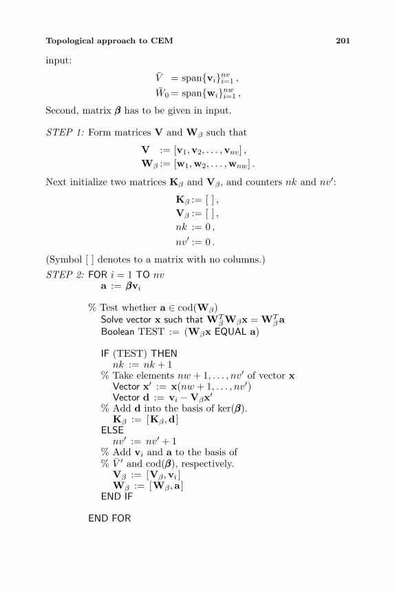
Topological approach to CEM 201
input:
V = spanvinvi=1 ,
W0 = spanwinwi=1 ,
Second, matrix βββ has to be given in input.
STEP 1: Form matrices V and Wβ such that
V := [v1,v2, . . . ,vnv] ,Wβ := [w1,w2, . . . ,wnw] .
Next initialize two matrices Kβ and Vβ, and counters nk and nv′:
Kβ := [ ] ,Vβ := [ ] ,nk := 0 ,
nv′ := 0 .
(Symbol [ ] denotes to a matrix with no columns.)
STEP 2: FOR i = 1 TO nva := βββvi
% Test whether a ∈ cod(Wβ)Solve vector x such that WT
βWβx = WTβ a
Boolean TEST := (Wβx EQUAL a)
IF (TEST) THENnk := nk + 1
% Take elements nw + 1, . . . , nv′ of vector xVector x′ := x(nw + 1, . . . , nv′)Vector d := vi −Vβx′
% Add d into the basis of ker(βββ).Kβ := [Kβ,d ]
ELSEnv′ := nv′ + 1
% Add vi and a to the basis of% V ′ and cod(βββ), respectively.
Vβ := [Vβ,vi ]Wβ := [Wβ,a ]
END IF
END FOR
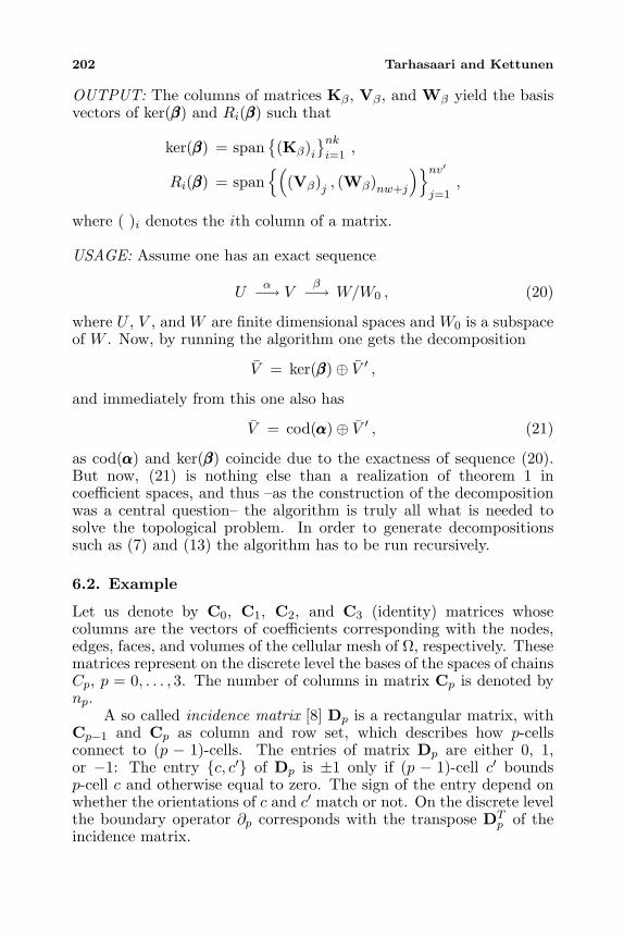
202 Tarhasaari and Kettunen
OUTPUT: The columns of matrices Kβ, Vβ, and Wβ yield the basisvectors of ker(βββ) and Ri(βββ) such that
ker(βββ) = span(Kβ)i
nki=1
,
Ri(βββ) = span(
(Vβ)j , (Wβ)nw+j
)nv′j=1
,
where ( )i denotes the ith column of a matrix.
USAGE: Assume one has an exact sequence
Uα−→ V
β−→ W/W0 , (20)
where U , V , and W are finite dimensional spaces and W0 is a subspaceof W . Now, by running the algorithm one gets the decomposition
V = ker(βββ)⊕ V ′ ,
and immediately from this one also has
V = cod(ααα)⊕ V ′ , (21)
as cod(ααα) and ker(βββ) coincide due to the exactness of sequence (20).But now, (21) is nothing else than a realization of theorem 1 incoefficient spaces, and thus –as the construction of the decompositionwas a central question– the algorithm is truly all what is needed tosolve the topological problem. In order to generate decompositionssuch as (7) and (13) the algorithm has to be run recursively.
6.2. Example
Let us denote by C0, C1, C2, and C3 (identity) matrices whosecolumns are the vectors of coefficients corresponding with the nodes,edges, faces, and volumes of the cellular mesh of Ω, respectively. Thesematrices represent on the discrete level the bases of the spaces of chainsCp, p = 0, . . . , 3. The number of columns in matrix Cp is denoted bynp.
A so called incidence matrix [8] Dp is a rectangular matrix, withCp−1 and Cp as column and row set, which describes how p-cellsconnect to (p − 1)-cells. The entries of matrix Dp are either 0, 1,or −1: The entry c, c′ of Dp is ±1 only if (p − 1)-cell c′ boundsp-cell c and otherwise equal to zero. The sign of the entry depend onwhether the orientations of c and c′ match or not. On the discrete levelthe boundary operator ∂p corresponds with the transpose DT
p of theincidence matrix.
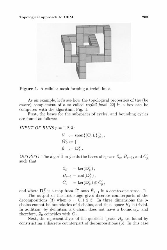
Topological approach to CEM 203
Figure 1. A cellular mesh forming a trefoil knot.
As an example, let’s see how the topological properties of the (beaware) complement of a so called trefoil knot [22] in a box can becomputed with the algorithm, Fig. 1.
First, the bases for the subspaces of cycles, and bounding cyclesare found as follows:
INPUT OF RUNS p = 1, 2, 3:
V := span(Cp)inpi=1 ,
W0 := [ ] ,
βββ := DTp .
OUTPUT: The algorithm yields the bases of spaces Zp, Bp−1, and C ′psuch that
Zp = ker(DTp ) ,
Bp−1 = cod(DTp ) ,
Cp = ker(DTp )⊕ C ′p ,
and where DTp is a map from C ′p onto Bp−1 in a one-to-one sense.
The output of the first stage gives discrete counterparts of thedecompositions (3) when p = 0, 1, 2, 3. In three dimensions the 3-chains cannot be boundaries of 4-chains, and thus, space B3 is trivial.In addition, by definition a 0-chain does not have a boundary, andtherefore, Z0 coincides with C0.
Next, the representatives of the quotient spaces Hp are found byconstructing a discrete counterpart of decompositions (6). In this case
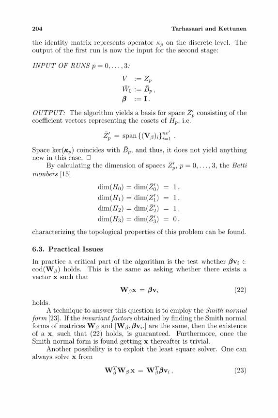
204 Tarhasaari and Kettunen
the identity matrix represents operator κp on the discrete level. Theoutput of the first run is now the input for the second stage:
INPUT OF RUNS p = 0, . . . , 3:
V := Zp
W0 := Bp ,
βββ := I .
OUTPUT: The algorithm yields a basis for space Z ′p consisting of thecoefficient vectors representing the cosets of Hp, i.e.
Z ′p = span (Vβ)inv′
i=1 .
Space ker(κκκp) coincides with Bp, and thus, it does not yield anythingnew in this case.
By calculating the dimension of spaces Z ′p, p = 0, . . . , 3, the Bettinumbers [15]
dim(H0) = dim(Z ′0) = 1 ,
dim(H1) = dim(Z ′1) = 1 ,
dim(H2) = dim(Z ′2) = 1 ,
dim(H3) = dim(Z ′3) = 0 ,
characterizing the topological properties of this problem can be found.
6.3. Practical Issues
In practice a critical part of the algorithm is the test whether βββvi ∈cod(Wβ) holds. This is the same as asking whether there exists avector x such that
Wβx = βββvi (22)
holds.A technique to answer this question is to employ the Smith normal
form [23]. If the invariant factors obtained by finding the Smith normalforms of matrices Wβ and [Wβ,βββvi.] are the same, then the existenceof a x, such that (22) holds, is guaranteed. Furthermore, once theSmith normal form is found getting x thereafter is trivial.
Another possibility is to exploit the least square solver. One canalways solve x from
WTβWβ x = WT
ββββvi , (23)
Topological approach to CEM 205
and then verify whether vector x fulfills also (22).If the coefficients are rational numbers, then arithmetics is exact.
In practice, however, computing with rational numbers (i.e., with pairsof integers) is inefficient when the matrices become large in size, andthus, one may have to use real numbers (in single or double precision)instead, But then, also an ε-test to check the equality between realnumbers is needed.
As the topological properties have nothing to do with thecardinality of the sets of nodes, edges, faces and volumes, in practice,computing time can be minimized by employing as coarse cellularmeshes as possible.
It is also useful to notice that the algorithm generalizes thespanning-tree techniques to construct trees and cotrees of graphs [24].
ACKNOWLEGMENT
We thank A. Bossavit and P. R. Kotiuga for ongoing discussions onrelated issues over the last years. This work was supported by theAcademy of Finland (project 34060).
REFERENCES
1. Yosida, K., Functional Analysis, Springer-Verlag, Berlin, 1980.2. Pierce, J. R., Symbols, Signals and Noise, Harper Torchbooks,
New York, 1965.3. Bossavit, A., “On the geometry of electromagnetism. (1):
Euclidean space,” J. Japan Soc. Appl. Electromagn. & Mech.,Vol. 6, No. 1, 17–28, 1998.
4. Bossavit, A., “On the geometry of electromagnetism. (2):Geometrical objects,” J. Japan Soc. Appl. Electromagn. & Mech.,Vol. 6, 114–123, 1998.
5. Bossavit, A., “On the geometry of electromagnetism. (3):Integration, Stokes’, Faraday’s laws,” J. Japan Soc. Appl.Electromagn. & Mech., Vol. 6, 233–240, 1998.
6. Bossavit, A., “On the geometry of electromagnetism. (4):Maxwell’s house,” J. Japan Soc. Appl. Electromagn. & Mech.,Vol. 6, 318–326, 1998.
7. Meyer, B., Object-Oriented Software Construction, Prentice Hall,Hertfordshire, UK, 1988.
8. Bossavit, A., Computational Electromagnetism, VariationalFormulations, Edge Elements, Complementarity, Academic Press,Boston, 1998.
206 Tarhasaari and Kettunen
9. de Rham, G., Differentiable Manifolds, Springer, 1984. (Trans-lated from the French).
10. Flanders, H., Differential Forms with Applications to the PhysicalSciences, Dover Publications, 1989.
11. Bossavit, A., “On non-linear magnetostatics: dual-complementary models and ‘mixed’ numerical methods,”Proc. of European Conf. on Math. in Ind., Glasgow, August 1988,J. Manby (ed.), 3–16, Teubner, Stuttgart, 1990.
12. Bossavit, A., “Differential forms and the computation of fieldsand forces in electromagnetism,” European J. Mech., B/Fluids,Vol. 10, No. 5, 474–488, 1991.
13. Lefschetz, S., Algebraic Topology, No. 27, A.M.S. ColloquimPublication, New York, 1942.
14. Cartan, H. and S. Eilenberg, Homological Algebra, PrincetonUniv. Press, 1952.
15. Hilton, P. J. and S. Wylie, Homology Theory, An Introductionto Algebraic Topology, Cambridge University Press, Cambridge,1965.
16. Hocking, J. G. and G. S. Young, Topology, Addison-Wesley Pub.Co., Reading, Mass., 1961.
17. Halmos, P. R., Naive Set Theory, Springer-Verlag, 1974.18. Kotiuga, P. R., “Hodge decompositions and computational
electromagnetics,” Ph.D. thesis, McGill University, Montreal,Canada, 1984.
19. Bossavit, A., “Most general ‘non-local’ boundary conditions forthe Maxwell equations in a bounded region,” Proceedings ofISEF’99 -9th Int. Symp. Elec. Magn. Fields. in Elec. Eng., Pavia,Italy, 1999.
20. Connor, P. E., “The Neumann’s problem for differential forms onRiemannian manifolds,” Memoirs of the AMS, No. 20, 1956.
21. Vick, J. W., Homology Theory, Academic Press, New York, 1973.22. Stillwell, J., Classical Topology and Combinatorial Group Theory,
Springer-Verlag, New York, 1980.23. Markus, H. and H. Minc, A Survey of Matrix Theory and Matrix
Inequalities, Allyn & Bacon, 1964.24. Kondo, K. and M. Iri, “On the theory of trees, cotrees, multitrees,
and multicotrees,” in RAAG Memoirs, II, No. Article A-VII, 220–261, 1959.
Progress In Electromagnetics Research, PIER 32, 207–245, 2001
FINITE ELEMENT-BASED ALGORITHMS TO MAKECUTS FOR MAGNETIC SCALAR POTENTIALS:TOPOLOGICAL CONSTRAINTS ANDCOMPUTATIONAL COMPLEXITY
P. W. Gross
Mathematical Sciences Research Institute1000 Centennial Drive, Berkeley, CA 94720, USA
P. R. Kotiuga
Department of Electrical and Computer EngineeringBoston University8 Saint Mary’s St., Boston, MA 02215, USA
Abstract—This paper outlines a generic algorithm to generate cutsfor magnetic scalar potentials in 3-dimensional multiply-connectedfinite element meshes. The algorithm is based on the algebraicstructures of (co)homology theory with differential forms anddeveloped in the context of the finite element method and finite elementdata structures. The paper also studies the computational complexityof the algorithm and examines how the topology of the region cancreate an obstruction to finding cuts inO(m2
0) time andO(m0) storage,where m0 is the number of vertices in the finite element mesh. We arguethat in a problem where there is no a priori data about the topology,the algorithm complexity is O(m2
0) in time and O(m4/30 ) in storage.
We indicate how this complexity can be achieved in implementationand optimized in the context of adaptive mesh refinement.
1 Introduction and Outline1.1 Electromagnetic and Numerical Scenario1.2 Are Cuts Worth the Trouble?1.3 Outline
208 Gross and Kotiuga
2 Definitions and Development of Topological Tools2.1 (Co)Homology Groups2.2 Poincare-Lefschetz Duality via Explicit Constructions2.3 The Isomorphism H1(R;Z) [R,S1]
3 The Variational Formulation of the Cuts Problem
4 The Connection between Finite Elements and Cuts4.1 The Role of Finite Elements in a Cuts Algorithm
5 Computation of 1-Cocycle Basis5.1 Definitions5.2 Formulation of a 1-Cocycle Generator Set5.3 Structure of Matrix Equation for Computing the 1-
Cocycle Generators5.3.1 Fixing Im (∂T1 )5.3.2 dim(N (U)) = β1(R)5.3.3 Sparsity of ∂T2 and U
5.3.4 Block Partition and Sparsity of the MatrixEquation
5.4 The Size of U22
6 Summary and Conclusions
Acknowledgment
Appendix A. Mesh-Counting ArithmeticA.1 The Euler Characteristic χ(R)A.2 The Details behind Table 1.2
Appendix B. Why Finite Element Analysis of MagneticFields Is Easy Once Cuts Are in Hand
References
1. INTRODUCTION AND OUTLINE
In this paper we consider a generic finite element-based algorithmto make cuts for magnetic scalar potentials and investigate howthe topological complexity of the three-dimensional region, whichconstitutes the domain of computation, affects the computationalcomplexity of the algorithm. The algorithm is based on standardfinite element theory with a novel computation required to deal with
Finite element-based algorithms to make cuts 209
topological constraints brought on by a scalar potential in a multiply-connected region. Thus, implementation can be designed to exploitpre-existing finite element software. Regardless of the topology of theregion, an algorithm can be implemented with O(m3
0) time complexityand O(m2
0) storage where m0 denotes the number of vertices in thefinite element discretization. However, in practice this is not usefulsince for large meshes since the cost of finding cuts would becomethe dominant factor in the magnetic field computation. In order tomake cuts worthwhile for problems such as nonlinear or time-varyingmagnetostatics, or in cases of complicated topology (e.g., braided,knotted, or linked conductor configurations, or even simple coils),an implementation of O(m2
0) time complexity and O(m0) storage isregarded as “ideal”.
The obstruction to ideal complexity is tied up in the structureof the fundamental group of the region. One implementation wasdesigned to have ideal complexity [29], however, the implementationhas heuristic assumptions which make it generally inadequate formaking cuts in regions for which the fundamental group of R hasa nontrivial commutator subgroup [13, 15]. This paper details analgorithm that can be implemented with O(m2
0) time complexity andO(m4/3
0 ) storage complexity given no more topological data than thatcontained in the finite element connection matrix.
While cuts algorithms have been discussed by several authors[7, 18, 37, 20, 21] some algorithms are based on the assumption thatcuts can be made in analogy to branch cuts in complex analysis.Such algorithms are limited to problems reducible to a planar problemand their success for this limited class of problems hinges on the factthat the topology of 2-d surfaces is “perfectly understood.” In threedimensions, intuition from Ampere’s law leads to a formal definitionof cuts in terms of a basis of the (abelian) homology groups of theregion [20, 21, 15], even though such cuts do not necessarily render theregion simply-connected [15]. The abelian nature of homology groupsmakes the problem computationally tractable while avoiding the subtleaspects of 3-dimensional topology which are trivial in two dimensions.
1.1. Electromagnetic and Numerical Scenario
The proper context for the algorithm of this paper is in variationalprinciples, the finite element method, and their connection to thetopology of the domain of computation. Before seeing how topologyenters the picture when going after a scalar potential, we define“magnetoquasistatics” as the class of electromagnetics problems wherethe magnetic field is described by a limiting case of Maxwell’s
210 Gross and Kotiuga
equations: ∫∂V
B · dS = 0 (1)
∫∂S
H · dl =∫SJ · n ds (2)
∫∂S′
E · dl = − d
dt
∫S′
B · n ds (3)
Here ∂V refers to the boundary of a region V and ∂S is the boundaryof a surface S. The displacement current ∂D/∂t in Ampere’s law isneglected and the current density vector J is assumed to be solenoidal.The magnetic flux density vector B is related to the magnetic fieldintensity H by B = B(H), or for linear isotropic media, B = µH. Thecurrent density J in conductors is related to the electric field intensityvector E by Ohm’s law: J = σE. Let R denote a region which is theintersection of the region where it is desired to compute the magneticfield and where the current density J is zero. In R,
curlH = 0, (4)
so that in terms of a scalar potential ψ,
H = gradψ (5)
in any contractible subset of R but ψ is globally multivalued as seenvia Ampere’s Law and illustrated in Figure 1.
Some scalar potential formulations sidestep the issue of themultivalued scalar potential by expressing the magnetic field as H =Hp + grad ψ, where Hp is a particular solution for the field obtained,say, from the Biot-Savart Law. However, in this case, if B = µH andµ → ∞, then H → 0 so that Hp = −grad ψ, leading to significantcancellation error for computation in regions where H 0 while a“total” scalar potential as in (5) eliminates cancellation error. Inaddition, integration of the Biot-Savart integral destroys the sparsityof any discretization. The particular solution, Hp, can be set to zero ina multiply-connected region when one introduces the notion of a “cut”which makes the scalar potential single-valued and if the software togenerate cuts does not require input from the user. This is a majorincentive for developing such algorithms.
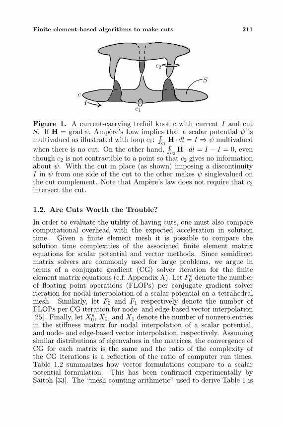
Finite element-based algorithms to make cuts 211
S
Ic1
c2
c
Figure 1. A current-carrying trefoil knot c with current I and cutS. If H = gradψ, Ampere’s Law implies that a scalar potential ψ ismultivalued as illustrated with loop c1:
∮c1
H ·dl = I ⇒ ψ multivaluedwhen there is no cut. On the other hand,
∮c2
H · dl = I − I = 0, eventhough c2 is not contractible to a point so that c2 gives no informationabout ψ. With the cut in place (as shown) imposing a discontinuityI in ψ from one side of the cut to the other makes ψ singlevalued onthe cut complement. Note that Ampere’s law does not require that c2intersect the cut.
1.2. Are Cuts Worth the Trouble?
In order to evaluate the utility of having cuts, one must also comparecomputational overhead with the expected acceleration in solutiontime. Given a finite element mesh it is possible to compare thesolution time complexities of the associated finite element matrixequations for scalar potential and vector methods. Since semidirectmatrix solvers are commonly used for large problems, we argue interms of a conjugate gradient (CG) solver iteration for the finiteelement matrix equations (c.f. Appendix A). Let F s
0 denote the numberof floating point operations (FLOPs) per conjugate gradient solveriteration for nodal interpolation of a scalar potential on a tetrahedralmesh. Similarly, let F0 and F1 respectively denote the number ofFLOPs per CG iteration for node- and edge-based vector interpolation[25]. Finally, let Xs
0 , X0, and X1 denote the number of nonzero entriesin the stiffness matrix for nodal interpolation of a scalar potential,and node- and edge-based vector interpolation, respectively. Assumingsimilar distributions of eigenvalues in the matrices, the convergence ofCG for each matrix is the same and the ratio of the complexity ofthe CG iterations is a reflection of the ratio of computer run times.Table 1.2 summarizes how vector formulations compare to a scalarpotential formulation. This has been confirmed experimentally bySaitoh [33]. The “mesh-counting arithmetic” used to derive Table 1 is
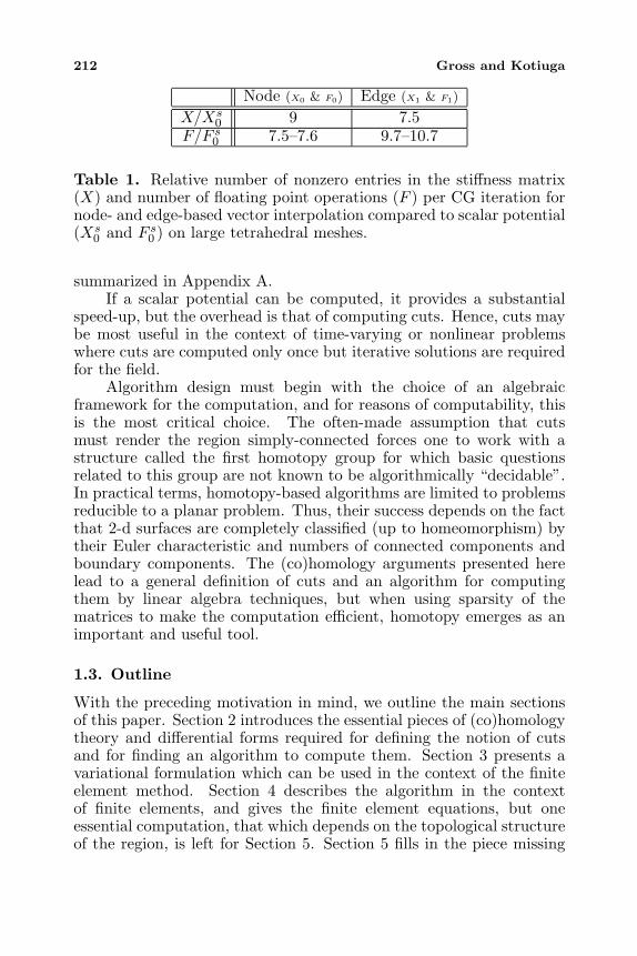
212 Gross and Kotiuga
Node (X0 & F0) Edge (X1 & F1)
X/Xs0 9 7.5
F/F s0 7.5–7.6 9.7–10.7
Table 1. Relative number of nonzero entries in the stiffness matrix(X) and number of floating point operations (F ) per CG iteration fornode- and edge-based vector interpolation compared to scalar potential(Xs
0 and F s0 ) on large tetrahedral meshes.
summarized in Appendix A.If a scalar potential can be computed, it provides a substantial
speed-up, but the overhead is that of computing cuts. Hence, cuts maybe most useful in the context of time-varying or nonlinear problemswhere cuts are computed only once but iterative solutions are requiredfor the field.
Algorithm design must begin with the choice of an algebraicframework for the computation, and for reasons of computability, thisis the most critical choice. The often-made assumption that cutsmust render the region simply-connected forces one to work with astructure called the first homotopy group for which basic questionsrelated to this group are not known to be algorithmically “decidable”.In practical terms, homotopy-based algorithms are limited to problemsreducible to a planar problem. Thus, their success depends on the factthat 2-d surfaces are completely classified (up to homeomorphism) bytheir Euler characteristic and numbers of connected components andboundary components. The (co)homology arguments presented herelead to a general definition of cuts and an algorithm for computingthem by linear algebra techniques, but when using sparsity of thematrices to make the computation efficient, homotopy emerges as animportant and useful tool.
1.3. Outline
With the preceding motivation in mind, we outline the main sectionsof this paper. Section 2 introduces the essential pieces of (co)homologytheory and differential forms required for defining the notion of cutsand for finding an algorithm to compute them. Section 3 presents avariational formulation which can be used in the context of the finiteelement method. Section 4 describes the algorithm in the contextof finite elements, and gives the finite element equations, but oneessential computation, that which depends on the topological structureof the region, is left for Section 5. Section 5 fills in the piece missing
Finite element-based algorithms to make cuts 213
from Section 4, describing an algorithm for finding the topologicalconstraints on the variational problem, and gives an analysis of thecomputational complexity of finding cuts. The overall process ofcomputing cuts is summarized in algorithm 1 and the algorithm ofSection 5 is summarized in algorithm 2. Two example problems areconsidered in order to illustrate the obstruction to O(n) complexity.Section 6 concludes with a summary of the main results, a review ofgeometric insights used to reduce the complexity of the algorithm, andsuggestions for future work.
2. DEFINITIONS AND DEVELOPMENT OFTOPOLOGICAL TOOLS
The subtleties of 3-dimensional electromagnetic boundary valueproblems are articulated through some special algebraic structures andrelationships between them. A good technical exposition of these isavailable from many sources [19, 10, 12, 35, 32], and there is a historicalcontext for their use in electromagnetic theory [27, 4], yet they seem tobe virtually absent from finite element algorithm design. We considerthe essential points here, reviewing three ingredients required for analgorithm:
(i) Homology and Cohomology groups: Homology groups are thestructures which algebraically encode information describingcurrent-linking (as in Ampere’s law) as well as cuts whilecohomology groups describe curl-free vector fields in the regionof interest.
(ii) Poincare-Lefschetz duality makes a connection between the curl-free fields and homology classes describing cuts, hence a definitionof cuts.
(iii) Isomorphism H1(R;Z) [R,S1]: A relationship between the curl-free fields and maps from the nonconducting region to the circlewhich guarantees existence of cuts with some desirable propertiesand is the key to a variational formulation of a cuts algorithm.
There are several advantages to formulating cuts in terms of(co)homology groups. One is that when a constructive proof of theexistence of cuts is phrased in terms of the formalism of a certainhomology theory, the proof gives way to a variational formulation fora cuts algorithm [21]. Another advantage is that various homologytheories give several ways to view cuts. Regarding a finite elementmesh as a simplicial complex [10], simplicial homology theory providesa framework for implementing an algorithm to make cuts andeven determines the most natural data structures as described in a
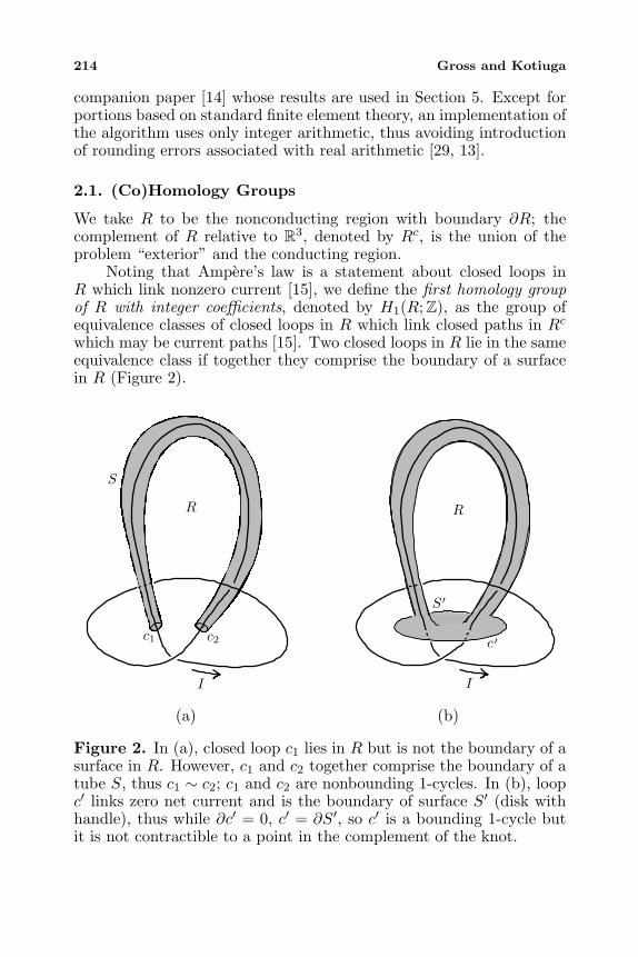
214 Gross and Kotiuga
companion paper [14] whose results are used in Section 5. Except forportions based on standard finite element theory, an implementation ofthe algorithm uses only integer arithmetic, thus avoiding introductionof rounding errors associated with real arithmetic [29, 13].
2.1. (Co)Homology Groups
We take R to be the nonconducting region with boundary ∂R; thecomplement of R relative to R3, denoted by Rc, is the union of theproblem “exterior” and the conducting region.
Noting that Ampere’s law is a statement about closed loops inR which link nonzero current [15], we define the first homology groupof R with integer coefficients, denoted by H1(R;Z), as the group ofequivalence classes of closed loops in R which link closed paths in Rc
which may be current paths [15]. Two closed loops in R lie in the sameequivalence class if together they comprise the boundary of a surfacein R (Figure 2).
S
R
I
c1 c2
I
R
S ′
c ′
(a) (b)
Figure 2. In (a), closed loop c1 lies in R but is not the boundary of asurface in R. However, c1 and c2 together comprise the boundary of atube S, thus c1 ∼ c2; c1 and c2 are nonbounding 1-cycles. In (b), loopc′ links zero net current and is the boundary of surface S′ (disk withhandle), thus while ∂c′ = 0, c′ = ∂S′, so c′ is a bounding 1-cycle butit is not contractible to a point in the complement of the knot.
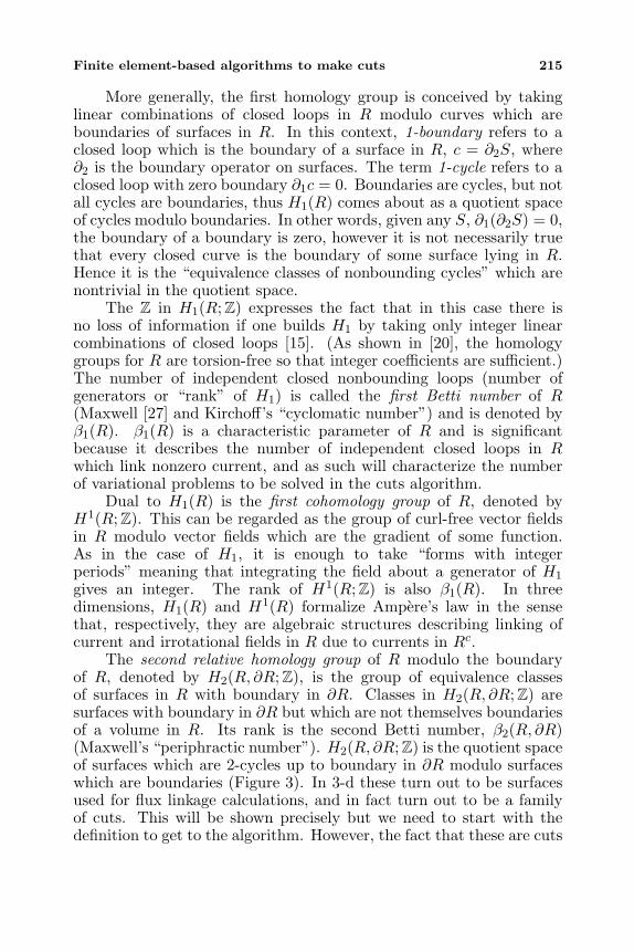
Finite element-based algorithms to make cuts 215
More generally, the first homology group is conceived by takinglinear combinations of closed loops in R modulo curves which areboundaries of surfaces in R. In this context, 1-boundary refers to aclosed loop which is the boundary of a surface in R, c = ∂2S, where∂2 is the boundary operator on surfaces. The term 1-cycle refers to aclosed loop with zero boundary ∂1c = 0. Boundaries are cycles, but notall cycles are boundaries, thus H1(R) comes about as a quotient spaceof cycles modulo boundaries. In other words, given any S, ∂1(∂2S) = 0,the boundary of a boundary is zero, however it is not necessarily truethat every closed curve is the boundary of some surface lying in R.Hence it is the “equivalence classes of nonbounding cycles” which arenontrivial in the quotient space.
The Z in H1(R;Z) expresses the fact that in this case there isno loss of information if one builds H1 by taking only integer linearcombinations of closed loops [15]. (As shown in [20], the homologygroups for R are torsion-free so that integer coefficients are sufficient.)The number of independent closed nonbounding loops (number ofgenerators or “rank” of H1) is called the first Betti number of R(Maxwell [27] and Kirchoff’s “cyclomatic number”) and is denoted byβ1(R). β1(R) is a characteristic parameter of R and is significantbecause it describes the number of independent closed loops in Rwhich link nonzero current, and as such will characterize the numberof variational problems to be solved in the cuts algorithm.
Dual to H1(R) is the first cohomology group of R, denoted byH1(R;Z). This can be regarded as the group of curl-free vector fieldsin R modulo vector fields which are the gradient of some function.As in the case of H1, it is enough to take “forms with integerperiods” meaning that integrating the field about a generator of H1
gives an integer. The rank of H1(R;Z) is also β1(R). In threedimensions, H1(R) and H1(R) formalize Ampere’s law in the sensethat, respectively, they are algebraic structures describing linking ofcurrent and irrotational fields in R due to currents in Rc.
The second relative homology group of R modulo the boundaryof R, denoted by H2(R, ∂R;Z), is the group of equivalence classesof surfaces in R with boundary in ∂R. Classes in H2(R, ∂R;Z) aresurfaces with boundary in ∂R but which are not themselves boundariesof a volume in R. Its rank is the second Betti number, β2(R, ∂R)(Maxwell’s “periphractic number”). H2(R, ∂R;Z) is the quotient spaceof surfaces which are 2-cycles up to boundary in ∂R modulo surfaceswhich are boundaries (Figure 3). In 3-d these turn out to be surfacesused for flux linkage calculations, and in fact turn out to be a familyof cuts. This will be shown precisely but we need to start with thedefinition to get to the algorithm. However, the fact that these are cuts
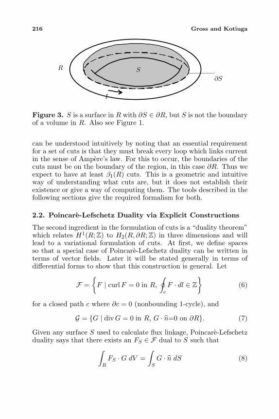
216 Gross and Kotiuga
SR
∂S
I
Figure 3. S is a surface in R with ∂S ∈ ∂R, but S is not the boundaryof a volume in R. Also see Figure 1.
can be understood intuitively by noting that an essential requirementfor a set of cuts is that they must break every loop which links currentin the sense of Ampere’s law. For this to occur, the boundaries of thecuts must be on the boundary of the region, in this case ∂R. Thus weexpect to have at least β1(R) cuts. This is a geometric and intuitiveway of understanding what cuts are, but it does not establish theirexistence or give a way of computing them. The tools described in thefollowing sections give the required formalism for both.
2.2. Poincare-Lefschetz Duality via Explicit Constructions
The second ingredient in the formulation of cuts is a “duality theorem”which relates H1(R;Z) to H2(R, ∂R;Z) in three dimensions and willlead to a variational formulation of cuts. At first, we define spacesso that a special case of Poincare-Lefschetz duality can be written interms of vector fields. Later it will be stated generally in terms ofdifferential forms to show that this construction is general. Let
F =F | curlF = 0 in R,
∮cF · dl ∈ Z
(6)
for a closed path c where ∂c = 0 (nonbounding 1-cycle), and
G = G | divG = 0 in R, G · n=0 on ∂R. (7)
Given any surface S used to calculate flux linkage, Poincare-Lefschetzduality says that there exists an FS ∈ F dual to S such that∫
RFS ·G dV =
∫SG · n dS (8)
Finite element-based algorithms to make cuts 217
for all G ∈ G. This illustrates the fact that the space of H1(R;Z) andH2(R, ∂R;Z) are dual spaces of the space of G vector fields subject tothe following equivalence relation:
G ∼ G′ if G′ = G + curlA (9)
for some A where n×A = 0 on ∂R.In the preceding, H1(R) has been articulated in terms of vector
fields for an intuitive understanding of the structure. However, thetheory is developed rigorously in terms of differential forms, so theseare introduced here in order to exploit the general theory. Looselyspeaking, differential forms are the objects appearing under integralsigns – integrands of p-fold integrals in an n-dimensional manifoldwhere 0 ≤ p ≤ n. They generalize the notion of a vector field andare a natural framework for engineering electromagnetics [19, 11]. Foran n-dimensional manifold Mn, the set of all p-dimensional regions cover which p-fold integrals are evaluated is denoted by Cp(Mn) whilethe set of all p-forms ω are denoted by Cp(Mn). Since Cp(Mn) andCp(Mn) are spaces with some algebraic structure, integration
∫cω (10)
can be regarded as a bilinear map∫: Cp(Mn)× Cp(Mn) −→ R (11)
(which, in a definite sense, is a nondegenerate bilinear pairing betweenthe spaces). In this context, the fundamental theorem of calculus,Gauss’ and Stokes’ theorems of multivariable calculus, and Green’stheorem in the plane are generalized by the Stokes theorem onmanifolds: ∫
cdω =
∫∂c
ω (12)
where ∂c ∈ Cp−1(Mn) is the boundary of c and the exterior derivativeoperator d takes p-forms to p+1-forms so as to satisfy Stokes’ theorem.Finally, there is a bilinear, associative, graded commutative productof forms, called the exterior product, which takes a p-form ω and aq-form η and gives a p + q-form ω ∧ η.
The introduction to homology groups hinted at the fact that∂p−1∂pc = 0. By a simple calculation, this combines with Stokes’theorem to show that p-forms satisfy dp+1dpω = 0 and motivates
218 Gross and Kotiuga
the following definition. A form µ is said to be closed if dµ = 0.In vector calculus, this amounts to saying that curl gradφ = 0 anddiv curlA = 0. Moreover, the existence of nonbounding cycles andStokes’ theorem also leads to the notion of exact forms: if µ = dωfor some ω, µ is said to be exact. While all exact p-forms are closed,not all closed forms are exact, so Hp is the quotient group of closedp-forms modulo exact p-forms. Formally, the coboundary operator isa map dp : Cp(M)→ Cp+1(M) and
Hp(M ;R) = ker dp/Im dp−1. (13)
In general, Poincare-Lefschetz duality says that for a compact,orientable n-dimensional manifold with boundary, Mn,
Hk(Mn;Z) Hn−k(Mn, ∂Mn;Z) (14)
for 0 ≤ k ≤ n. This theorem is true for any abelian coefficientgroup, but it is enough to deal with integer coefficients here. Inthe case of n = 3, duality establishes a one-to-one correspondencebetween classes in H1(R;Z) and classes in H2(R, ∂R;Z). In the contextof magnetoquasistatics, these are, respectively, equivalence classes ofmagnetic fields and equivalence classes of surfaces for flux linkagecalculations.
To develop a formal definition of a “cut” we need the notion ofthe Poincare-Lefschetz dual of a submanifold. Given an n-dimensionalcompact, oriented manifold Mn with boundary, a closed oriented n−k-dimensional submanifold S of Mn, and a closed n − k-form ω whoserestriction to ∂M is zero, the Poincare-Lefschetz dual of S is a closedk-form ηS such that [6] ∫
Mn
ω ∧ ηS =∫Sω. (15)
This is a generalized statement of equation (8). When subjected tothe (co)homology equivalence relations, the bilinear pairings on bothsides of equation (15) become nondegenerate bilinear pairings betweenHk(Mn) and Hn−k(Mn, ∂Mn) on the left, and Hn−k(Mn, ∂Mn)and Hn−k(M,∂M) on the right. Thus equation (14) arises sinceHn−k(Mn, ∂Mn) is the dual space to both spaces. In other words,for the homology class [S] ∈ Hn−k(Mn, ∂Mn) associated with asubmanifold S ∈ Mn, there is an associated unique cohomology class[ηS ] ∈ Hk(Mn). As a consequence of Poincare-Lefschetz duality, cutscan be defined as representatives of classes in H2(R, ∂R;Z). Theisomorphism discussed below allows us to restrict our attention to cutswhich are embedded manifolds in R, and at the same time gives a wayof computing these cuts through a variational problem.
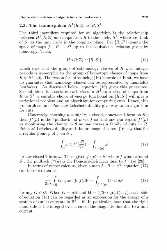
Finite element-based algorithms to make cuts 219
2.3. The Isomorphism H1(R;Z) [R,S1]
The third ingredient required for an algorithm is the relationshipbetween H1(R;Z) and maps from R to the circle, S1, where we thinkof S1 as the unit circle in the complex plane. Let [R,S1] denote thespace of maps f : R → S1 up to the equivalence relation given byhomotopy. Then,
H1(R;Z) [R,S1] (16)
which says that the group of cohomology classes of R with integerperiods is isomorphic to the group of homotopy classes of maps fromR to S1 [20]. The reason for introducing (16) is twofold: First, we haveno guarantee that homology classes can be represented by manifolds(surfaces). As discussed below, equation (16) gives this guarantee.Second, since it associates each class in H1 to a class of maps fromR to S1, a suitable choice of energy functional on [R,S1] will give avariational problem and an algorithm for computing cuts. Hence, thisisomorphism and Poincare-Lefschetz duality give way to an algorithmfor cuts.
Concretely, choosing µ = dθ/2π, a closed, nonexact 1-form on S1,then f∗(µ) is the “pullback” of µ via f so that one can regard f∗(µ)as monitoring the change in θ as one covers a family of cuts in R.Poincare-Lefschetz duality and the preimage theorem [16] say that fora regular point p of f on S1,
∫Rω ∧ f∗(
dθ
2π) =
∫f−1(p)
ω (17)
for any closed 2-form ω. Thus, given f : R→ S1 where f winds aroundS1, the pullback f∗(µ) is the Poincare-Lefschetz dual to f−1(p) [20].
In terms of vector calculus, given a map f : R→ S1, equation (17)can be re-written as
12πi
∫RG · grad (ln f)dV =
∫f−1(p)
G · n dS (18)
for any G ∈ G. When G = µH and H = 1/2πi grad (ln f), each sideof equation (18) can be regarded as an expression for the energy of asystem of (unit) currents in R3 −R. In particular, note that the righthand side is the integral over a cut of the magnetic flux due to a unitcurrent.
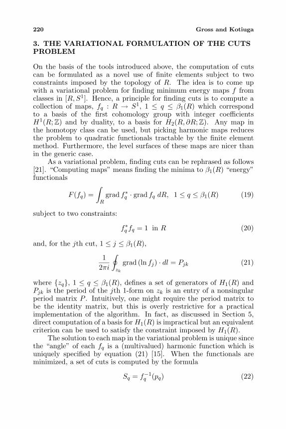
220 Gross and Kotiuga
3. THE VARIATIONAL FORMULATION OF THE CUTSPROBLEM
On the basis of the tools introduced above, the computation of cutscan be formulated as a novel use of finite elements subject to twoconstraints imposed by the topology of R. The idea is to come upwith a variational problem for finding minimum energy maps f fromclasses in [R,S1]. Hence, a principle for finding cuts is to compute acollection of maps, fq : R → S1, 1 ≤ q ≤ β1(R) which correspondto a basis of the first cohomology group with integer coefficientsH1(R;Z) and by duality, to a basis for H2(R, ∂R;Z). Any map inthe homotopy class can be used, but picking harmonic maps reducesthe problem to quadratic functionals tractable by the finite elementmethod. Furthermore, the level surfaces of these maps are nicer thanin the generic case.
As a variational problem, finding cuts can be rephrased as follows[21]. “Computing maps” means finding the minima to β1(R) “energy”functionals
F (fq) =∫R
grad f∗q · grad fq dR, 1 ≤ q ≤ β1(R) (19)
subject to two constraints:
f∗q fq = 1 in R (20)
and, for the jth cut, 1 ≤ j ≤ β1(R),
12πi
∮zk
grad (ln fj) · dl = Pjk (21)
where zq, 1 ≤ q ≤ β1(R), defines a set of generators of H1(R) andPjk is the period of the jth 1-form on zk is an entry of a nonsingularperiod matrix P . Intuitively, one might require the period matrix tobe the identity matrix, but this is overly restrictive for a practicalimplementation of the algorithm. In fact, as discussed in Section 5,direct computation of a basis for H1(R) is impractical but an equivalentcriterion can be used to satisfy the constraint imposed by H1(R).
The solution to each map in the variational problem is unique sincethe “angle” of each fq is a (multivalued) harmonic function which isuniquely specified by equation (21) [15]. When the functionals areminimized, a set of cuts is computed by the formula
Sq = f−1q (pq) (22)
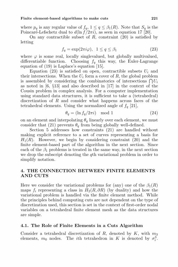
Finite element-based algorithms to make cuts 221
where pq is any regular value of fq, 1 ≤ q ≤ β1(R). Note that Sq is thePoincare-Lefschetz dual to d(ln f/2πi), as seen in equation 17 [20].
On any contractible subset of R, constraint (20) is satisfied byletting
fq = exp(2πiϕ), 1 ≤ q ≤ β1 (23)
where ϕ is some real, locally singlevalued, but globally multivalued,differentiable function. Choosing fq this way, the Euler-Lagrangeequation of (19) is Laplace’s equation [15].
Equation (23) is satisfied on open, contractible subsets Ui andtheir intersections. When the Ui form a cover of R, the global problemis assembled by considering the combinatorics of intersections
⋂Ui
as noted in [6, §13] and also described in [17] in the context of theCousin problem in complex analysis. For a computer implementationusing standard data structures, it is sufficient to take a (tetrahedral)discretization of R and consider what happens across faces of thetetrahedral elements. Using the normalized angle of fq [21],
θq = (ln fq/2πi) mod 1 (24)
on an element and interpolating θq linearly over each element, we mustconsider that (21) prevents θq from being globally well-defined.
Section 5 addresses how constraints (21) are handled withoutmaking explicit reference to a set of curves representing a basis forH1(R). However, we begin by considering constraint (20) and thefinite element-based part of the algorithm in the next section. Sinceeach of the β1 problems is treated in the same way, in the next sectionwe drop the subscript denoting the qth variational problem in order tosimplify notation.
4. THE CONNECTION BETWEEN FINITE ELEMENTSAND CUTS
Here we consider the variational problems for (any) one of the β1(R)maps fi representing a class in H2(R, ∂R) (by duality) and how thevariational problem is handled via the finite element method. Whilethe principles behind computing cuts are not dependent on the type ofdiscretization used, this section is set in the context of first-order nodalvariables on a tetrahedral finite element mesh as the data structuresare simple.
4.1. The Role of Finite Elements in a Cuts Algorithm
Consider a tetrahedral discretization of R, denoted by K, with m3
elements, m0 nodes. The ith tetrahedron in K is denoted by σ3i .
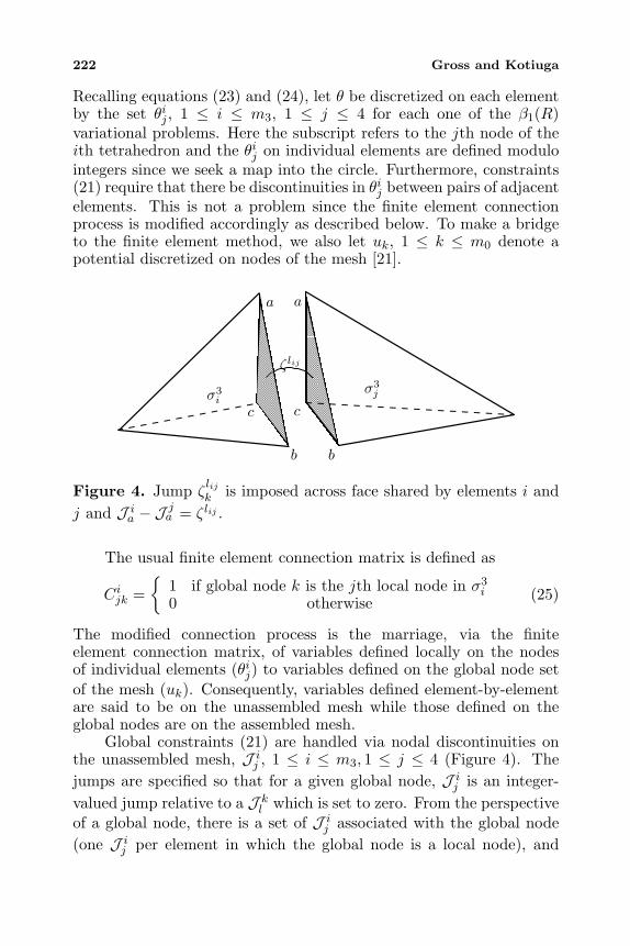
222 Gross and Kotiuga
Recalling equations (23) and (24), let θ be discretized on each elementby the set θij , 1 ≤ i ≤ m3, 1 ≤ j ≤ 4 for each one of the β1(R)variational problems. Here the subscript refers to the jth node of theith tetrahedron and the θij on individual elements are defined modulointegers since we seek a map into the circle. Furthermore, constraints(21) require that there be discontinuities in θij between pairs of adjacentelements. This is not a problem since the finite element connectionprocess is modified accordingly as described below. To make a bridgeto the finite element method, we also let uk, 1 ≤ k ≤ m0 denote apotential discretized on nodes of the mesh [21].
a
σ3jσ3
i
b
a
b
c
ζlij
c
Figure 4. Jump ζlijk is imposed across face shared by elements i and
j and J ia − J ja = ζ lij .
The usual finite element connection matrix is defined as
Cijk =
1 if global node k is the jth local node in σ3
i0 otherwise (25)
The modified connection process is the marriage, via the finiteelement connection matrix, of variables defined locally on the nodesof individual elements (θij) to variables defined on the global node setof the mesh (uk). Consequently, variables defined element-by-elementare said to be on the unassembled mesh while those defined on theglobal nodes are on the assembled mesh.
Global constraints (21) are handled via nodal discontinuities onthe unassembled mesh, J ij , 1 ≤ i ≤ m3, 1 ≤ j ≤ 4 (Figure 4). Thejumps are specified so that for a given global node, J ij is an integer-valued jump relative to a J kl which is set to zero. From the perspectiveof a global node, there is a set of J ij associated with the global node(one J ij per element in which the global node is a local node), and
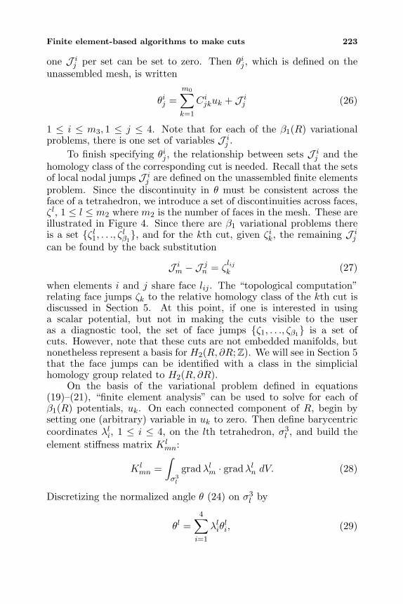
Finite element-based algorithms to make cuts 223
one J ij per set can be set to zero. Then θij , which is defined on theunassembled mesh, is written
θij =m0∑k=1
Cijkuk + J ij (26)
1 ≤ i ≤ m3, 1 ≤ j ≤ 4. Note that for each of the β1(R) variationalproblems, there is one set of variables J ij .
To finish specifying θij , the relationship between sets J ij and thehomology class of the corresponding cut is needed. Recall that the setsof local nodal jumps J ij are defined on the unassembled finite elementsproblem. Since the discontinuity in θ must be consistent across theface of a tetrahedron, we introduce a set of discontinuities across faces,ζ l, 1 ≤ l ≤ m2 where m2 is the number of faces in the mesh. These areillustrated in Figure 4. Since there are β1 variational problems thereis a set ζ l1, . . ., ζ lβ1
, and for the kth cut, given ζik, the remaining J ijcan be found by the back substitution
J im − J jn = ζlijk (27)
when elements i and j share face lij . The “topological computation”relating face jumps ζk to the relative homology class of the kth cut isdiscussed in Section 5. At this point, if one is interested in usinga scalar potential, but not in making the cuts visible to the useras a diagnostic tool, the set of face jumps ζ1, . . ., ζβ1 is a set ofcuts. However, note that these cuts are not embedded manifolds, butnonetheless represent a basis for H2(R, ∂R;Z). We will see in Section 5that the face jumps can be identified with a class in the simplicialhomology group related to H2(R, ∂R).
On the basis of the variational problem defined in equations(19)–(21), “finite element analysis” can be used to solve for each ofβ1(R) potentials, uk. On each connected component of R, begin bysetting one (arbitrary) variable in uk to zero. Then define barycentriccoordinates λli, 1 ≤ i ≤ 4, on the lth tetrahedron, σ3
l , and build theelement stiffness matrix K l
mn:
K lmn =
∫σ3l
gradλlm · gradλln dV. (28)
Discretizing the normalized angle θ (24) on σ3l by
θl =4∑i=1
λliθli, (29)
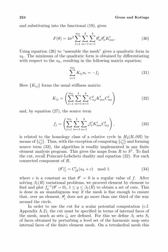
224 Gross and Kotiuga
and substituting into the functional (19), gives
F (θ) = 4π2m3∑l=1
4∑m=1
4∑n=1
θlmθlnK
lmn. (30)
Using equation (26) to “assemble the mesh” gives a quadratic form inuk. The minimum of the quadratic form is obtained by differentiatingwith respect to the uk, resulting in the following matrix equation:
m0∑i=1
Kijui = −fj (31)
Here Kij forms the usual stiffness matrix:
Kij =
(m3∑l=1
4∑m=1
4∑n=1
C lnjK
lmnC
lmi
)(32)
and, by equation (27), the source term
fj =
(m3∑l=1
4∑m=1
4∑n=1
J lnK lmnC
lmj
), (33)
is related to the homology class of a relative cycle in H2(R, ∂R) bymeans of ζij. Thus, with the exception of computing ζij and formingsource term (33), the algorithm is readily implemented in any finiteelement analysis program. This gives the maps from R to S1. To findthe cut, recall Poincare-Lefschetz duality and equation (22). For eachconnected component of R,
(θ′)ij = Cijk(uk + c) mod 1. (34)
where c is a constant so that θ′ = 0 is a regular value of f . Aftersolving β1(R) variational problems, we proceed element by element tofind and plot f−1
q (θ′ = 0), 1 ≤ q ≤ β1(R) to obtain a set of cuts. Thisis done in an unambiguous way if the mesh is fine enough to ensurethat, over an element, θij does not go more than one third of the wayaround the circle.
In order to use the cut for a scalar potential computation (c.f.Appendix A.2), the cut must be specified in terms of internal faces ofthe mesh, much as sets ζi are defined. For this we define β1 sets Siof faces obtained by perturbing a level set of the harmonic map ontointernal faces of the finite element mesh. On a tetrahedral mesh this
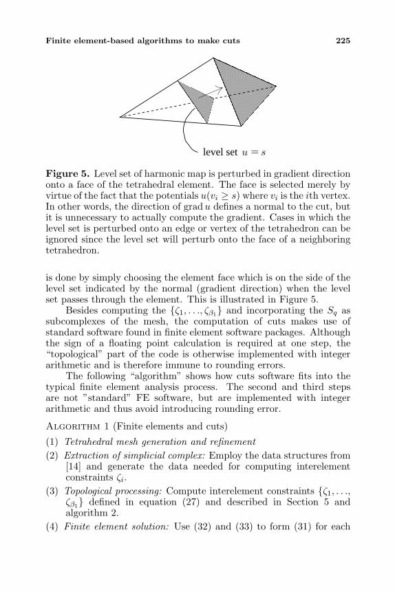
Finite element-based algorithms to make cuts 225
u = slevel set
Figure 5. Level set of harmonic map is perturbed in gradient directiononto a face of the tetrahedral element. The face is selected merely byvirtue of the fact that the potentials u(vi ≥ s) where vi is the ith vertex.In other words, the direction of gradu defines a normal to the cut, butit is unnecessary to actually compute the gradient. Cases in which thelevel set is perturbed onto an edge or vertex of the tetrahedron can beignored since the level set will perturb onto the face of a neighboringtetrahedron.
is done by simply choosing the element face which is on the side of thelevel set indicated by the normal (gradient direction) when the levelset passes through the element. This is illustrated in Figure 5.
Besides computing the ζ1, . . ., ζβ1 and incorporating the Sq assubcomplexes of the mesh, the computation of cuts makes use ofstandard software found in finite element software packages. Althoughthe sign of a floating point calculation is required at one step, the“topological” part of the code is otherwise implemented with integerarithmetic and is therefore immune to rounding errors.
The following “algorithm” shows how cuts software fits into thetypical finite element analysis process. The second and third stepsare not ”standard” FE software, but are implemented with integerarithmetic and thus avoid introducing rounding error.
Algorithm 1 (Finite elements and cuts)
(1) Tetrahedral mesh generation and refinement(2) Extraction of simplicial complex: Employ the data structures from
[14] and generate the data needed for computing interelementconstraints ζi.
(3) Topological processing: Compute interelement constraints ζ1, . . .,ζβ1 defined in equation (27) and described in Section 5 andalgorithm 2.
(4) Finite element solution: Use (32) and (33) to form (31) for each
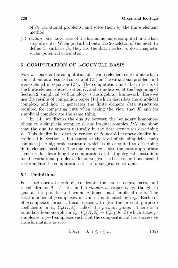
226 Gross and Kotiuga
of β1 variational problems, and solve them by the finite elementmethod.
(5) Obtain cuts: Level sets of the harmonic maps computed in the laststep are cuts. When perturbed onto the 2-skeleton of the mesh todefine β1 surfaces Si, they are the data needed to do a magneticscalar potential calculation.
5. COMPUTATION OF 1-COCYCLE BASIS
Now we consider the computation of the interelement constraints whichcome about as a result of constraint (21) on the variational problem andwere defined in equation (27). The computation must be in terms ofthe finite element discretization K, and as indicated at the beginning ofSection 2, simplicial (co)homology is the algebraic framework. Here weuse the results of companion paper [14] which describes the simplicialcomplex, and how it generates the finite element data structuresrequired for computing cuts when taking the view that K and itssimplicial complex are the same thing.
In [14], we discuss the duality between the boundary homomor-phism on a simplicial complex K and its dual complex DK and showthat the duality appears naturally in the data structures describingK. This duality is a discrete version of Poincare-Lefschetz duality in-troduced in Section 2, but stated at the level of the simplicial chaincomplex (the algebraic structure which is most suited to describingfinite element meshes). The dual complex is also the most appropriatestructure for describing the computation of the topological constraintsfor the variational problem. Below we give the basic definitions neededto formulate the computation of the topological constraints.
5.1. Definitions
For a tetrahedral mesh K, se denote the nodes, edges, faces, andtetrahedra as 0-, 1-, 2-, and 3-simplexes, respectively, though ingeneral it is possible to have an n-dimensional simplicial mesh. Thetotal number of p-simplexes in a mesh is denoted by mp. Each setof p-simplexes forms a linear space with (for the present purpose)coefficients in Z, Cp(K;Z), called the p-chain group. There is aboundary homomorphism ∂p : Cp(K;Z)→ Cp−1(K;Z) which takes p-simplexes to p−1-simplexes such that the composition of two successivetransformations is zero:
∂i∂i+1 = 0, 1 ≤ i ≤ n. (35)
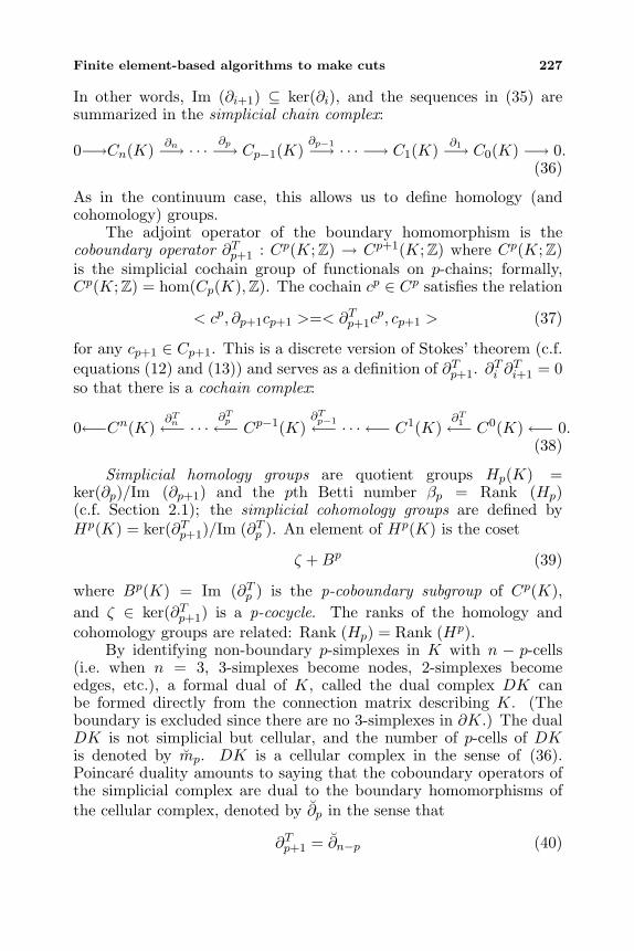
Finite element-based algorithms to make cuts 227
In other words, Im (∂i+1) ⊆ ker(∂i), and the sequences in (35) aresummarized in the simplicial chain complex:
0−→Cn(K) ∂n−→ · · · ∂p−→ Cp−1(K)∂p−1−→ · · · −→ C1(K) ∂1−→ C0(K) −→ 0.
(36)
As in the continuum case, this allows us to define homology (andcohomology) groups.
The adjoint operator of the boundary homomorphism is thecoboundary operator ∂Tp+1 : Cp(K;Z) → Cp+1(K;Z) where Cp(K;Z)is the simplicial cochain group of functionals on p-chains; formally,Cp(K;Z) = hom(Cp(K),Z). The cochain cp ∈ Cp satisfies the relation
< cp, ∂p+1cp+1 >=< ∂Tp+1cp, cp+1 > (37)
for any cp+1 ∈ Cp+1. This is a discrete version of Stokes’ theorem (c.f.equations (12) and (13)) and serves as a definition of ∂Tp+1. ∂Ti ∂
Ti+1 = 0
so that there is a cochain complex:
0←−Cn(K)∂Tn←− · · ·
∂Tp←− Cp−1(K)∂Tp−1←− · · · ←− C1(K)
∂T1←− C0(K)←− 0.(38)
Simplicial homology groups are quotient groups Hp(K) =ker(∂p)/Im (∂p+1) and the pth Betti number βp = Rank (Hp)(c.f. Section 2.1); the simplicial cohomology groups are defined byHp(K) = ker(∂Tp+1)/Im (∂Tp ). An element of Hp(K) is the coset
ζ + Bp (39)
where Bp(K) = Im (∂Tp ) is the p-coboundary subgroup of Cp(K),and ζ ∈ ker(∂Tp+1) is a p-cocycle. The ranks of the homology andcohomology groups are related: Rank (Hp) = Rank (Hp).
By identifying non-boundary p-simplexes in K with n − p-cells(i.e. when n = 3, 3-simplexes become nodes, 2-simplexes becomeedges, etc.), a formal dual of K, called the dual complex DK canbe formed directly from the connection matrix describing K. (Theboundary is excluded since there are no 3-simplexes in ∂K.) The dualDK is not simplicial but cellular, and the number of p-cells of DKis denoted by mp. DK is a cellular complex in the sense of (36).Poincare duality amounts to saying that the coboundary operators ofthe simplicial complex are dual to the boundary homomorphisms ofthe cellular complex, denoted by ∂p in the sense that
∂Tp+1 = ∂n−p (40)
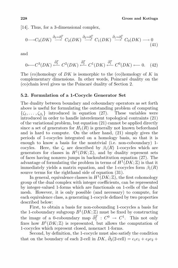
228 Gross and Kotiuga
[14]. Thus, for a 3-dimensional complex,
0−→C3(DK)∂3=∂T1−→ C2(DK)
∂2=∂T2−→ C1(DK)∂1=∂T3−→ C0(DK) −→ 0
(41)
and
0←−C3(DK)∂T3←− C2(DK)
∂T2←− C1(DK)∂T1←− C0(DK)←− 0. (42)
The (co)homology of DK is isomorphic to the (co)homology of K incomplementary dimensions. In other words, Poincare duality on the(co)chain level gives us the Poincare duality of Section 2.
5.2. Formulation of a 1-Cocycle Generator Set
The duality between boundary and coboundary operators as set forthabove is useful for formulating the outstanding problem of computingζ1, . . . , ζβ1 introduced in equation (27). These variables wereintroduced in order to handle interelement topological contraints (21)of the variational problem, but equation (21) cannot be applied directlysince a set of generators for H1(R) is generally not known beforehandand is hard to compute. On the other hand, (21) simply gives theperiods of 1-cocycles integrated on a homology basis, so that it isenough to know a basis for the nontrivial (i.e. non-coboundary) 1-cocyles. Here, the ζi are described by β1(R) 1-cocycles which aregenerators for classes in H1(DK;Z), and by duality represent setsof faces having nonzero jumps in backsubstitution equation (27). Theadvantage of formulating the problem in terms of H1(DK;Z) is that itimmediately yields a matrix equation, and the 1-cocycles form β1(R)source terms for the righthand side of equation (31).
In general, equivalence classes in H1(DK;Z), the first cohomologygroup of the dual complex with integer coefficients, can be representedby integer-valued 1-forms which are functionals on 1-cells of the dualmesh. However, it is only possible (and necessary) to compute, foreach equivalence class, a generating 1-cocycle defined by two propertiesdescribed below:
First, to obtain a basis for non-cobounding 1-cocycles a basis forthe 1-coboundary subgroup B1(DK;Z) must be fixed by constructingthe image of a 0-coboundary map ∂T1 : C0 → C1. This not onlyfixes how B1(DK;Z) is represented, but allows the computation of1-cocycles which represent closed, nonexact 1-forms.
Second, by definition, the 1-cocycle must also satisfy the conditionthat on the boundary of each 2-cell in DK, ∂2(2-cell) = ε1e1 + ε2e2 +
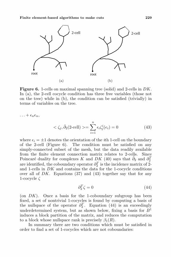
Finite element-based algorithms to make cuts 229
2-cell 2-cell
root root
(a) (b)
Figure 6. 1-cells on maximal spanning tree (solid) and 2-cells in DK.In (a), the 2-cell cocycle condition has three free variables (those noton the tree) while in (b), the condition can be satisfied (trivially) interms of variables on the tree.
. . . + εnen,
< ζj , ∂2(2-cell) >=n∑i=1
εiζij(ei) = 0 (43)
where εi = ±1 denotes the orientation of the ith 1-cell on the boundaryof the 2-cell (Figure 6). The condition must be satisfied on anysimply-connected subset of the mesh, but the data readily availablefrom the finite element connection matrix relates to 2-cells. SincePoincare duality for complexes K and DK (40) says that ∂2 and ∂T2are identified, the coboundary operator ∂T2 is the incidence matrix of 2-and 1-cells in DK and contains the data for the 1-cocycle conditionsover all of DK. Equations (37) and (43) together say that for any1-cocycle ζ
∂T2 ζ = 0 (44)
(on DK). Once a basis for the 1-coboundary subgroup has beenfixed, a set of nontrivial 1-cocycles is found by computing a basis ofthe nullspace of the operator ∂T2 . Equation (44) is an exceedinglyunderdetermined system, but as shown below, fixing a basis for B1
induces a block partition of the matrix, and reduces the computationto a block whose nullspace rank is precisely β1(R).
In summary there are two conditions which must be satisfied inorder to find a set of 1-cocycles which are not coboundaries:
230 Gross and Kotiuga
(i) A basis for B1 must be fixed by considering the image of a map∂T1 : C0 −→ C1.
(ii) The 1-cocycles must independently satisfy the 1-cocycle conditionon each 2-cell of the mesh.
5.3. Structure of Matrix Equation for Computing the1-Cocycle Generators
The strategy outlined above amounts to constructing bases for Im (∂T1 )and ker(∂T2 ) (subject to Im (∂T1 ) = 0) in the semi-exact sequence (42).When Im (∂T1 ) is annihilated, the surviving piece of ker(∂T2 ) gives abasis for 1-cohomology generators. In this section we give a methodfor constructing the required bases while retaining the sparsity of ∂T2and show how the construction yields a natural block partition of thematrix.
The arguments of this section have the same motivation astechniques of electrical circuit analysis. The rank argument ofSection 5.3.2 is a formalization of a familiar equation which relates thenumber of free variables nfree to the numbers of Kirchhoff current law(node) and Kirchhoff voltage law (loop) equations (nKCL and nKV L):
nKCL + nKV L − β0 = nfree (45)
where β0 = Rank (H0) is the number of connected components of themesh or circuit (c.f. Appendix A.1 for a different guise of the equationabove).
5.3.1. Fixing Im (∂T1 )
To fix B1(DK), we construct a map ∂T1 which satisfies the Stokes’equation (37) which for this case says < c0, ∂e >=< ∂T c0, e > wheree ∈ C1(DK), c0 ∈ C0(DK). Defining c0 on vertices of DK andbuilding a maximal tree on the 1-skeleton of DK fixes a basis forB1 = Im (∂T1 ω) up to a constant on a single vertex on each connectedcomponent of DK by associating each vertex (functional) with an edge(functional) on the 1-skeleton. Note that there are m0−β0 1-cells on themaximal tree, the same as the rank of Im (∂T1 ). Since the coboundarysubgroup is annihilated in the equivalence relation for cohomology, thevariables of ζi corresponding to edges on the maximal tree can be setto zero. Below we see that this reduces the number of free variablesenough to permit computation of an appropriate set of independentnullvectors of ∂T2 .
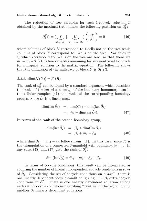
Finite element-based algorithms to make cuts 231
The reduction of free variables for each 1-cocycle solution ζiobtained by the maximal tree induces the following partition on ∂T2 :
∂T2 ζi = ( T︸︷︷︸m0−β0
| U︸︷︷︸m1−m0+β0
)(
0TζU
)= 0 (46)
where columns of block U correspond to 1-cells not on the tree whilecolumns of block T correspond to 1-cells on the tree. Variables inζi which correspond to 1-cells on the tree are zero, so that there arem1−m0+β0(DK) free variables remaining for any nontrivial 1-cocycle(or nullspace) solution to the matrix equation. The following showsthat the dimension of the nullspace of block U is β1(R).
5.3.2. dim(N (U)) = β1(R)
The rank of ∂T2 can be found by a standard argument which considersthe ranks of the kernel and image of the boundary homomorphism inthe cellular complex (41) and ranks of the corresponding homologygroups. Since ∂2 is a linear map,
dim(Im ∂2) = dim(C2)− dim(ker ∂2)
= m2 − dim(ker ∂2). (47)
In terms of the rank of the second homology group,
dim(ker ∂2) = β2 + dim(Im ∂3)= β2 + m3 − β3 (48)
where dim(∂3) = m3 − β3 follows from (41). In this case, since K isthe triangulation of a connected 3-manifold with boundary, β3 = 0. Inany case, (48) and (47) give the rank of ∂T2 :
dim(Im ∂2) = m2 − m3 − β2 + β3. (49)
In terms of cocycle conditions, this result can be interpreted ascounting the number of linearly independent cocycle conditions in rowsof ∂2. Considering the set of cocycle conditions on a 3-cell, there isone linearly dependent cocycle condition, giving m3−β3 extra cocycleconditions in ∂T2 . There is one linearly dependent equation amongeach set of cocycle conditions describing “cavities” of the region, givinganother β2 linearly dependent equations.
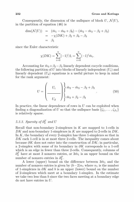
232 Gross and Kotiuga
Consequently, the dimension of the nullspace of block U , N (U),in the partition of equation (46) is
dim(N (U)) = (m1 − m0 + β0)− (m2 − m3 − β2 + β3)= −χ(DK) + β2 + β0 − β3
= β1
since the Euler characteristic
χ(DK) =n∑i=0
(−1)iβi =n∑i=0
(−1)imi.
Accounting for m3+β2−β3 linearly dependent cocycle conditions,the following partition of U into blocks of linearly independent (Ui) andlinearly dependent (Ud) equations is a useful picture to keep in mindfor the rank argument:
U =
Ui
Ud
m2 − m3 − β2 + β3
m3 + β2 − β3
. (50)
In practice, the linear dependence of rows in U can be exploited whenfinding a diagonalization of U so that the nullspace basis ζ1, . . . , ζβ1is relatively sparse.
5.3.3. Sparsity of ∂T2 and U
Recall that non-boundary 2-simplexes in K are mapped to 1-cells inDK and non-boundary 1-simplexes in K are mapped to 2-cells in DK.In K, the boundary of every 2-simplex has three 1-simplexes so that inDK each 1-cell is in at most three 2-cells. The inequality comes aboutbecause ∂K does not enter into the construction of DK; in particular,a 2-simplex with some of its boundary in ∂K corresponds to a 1-cellwhich is an edge in fewer than three 2-cells. Consequently, columns of∂T2 have at most 3 nonzero entries, or 3m1 is an upper bound on thenumber of nonzero entries in ∂T2 .
A lower (upper) bound on the difference between 3m1 and thenumber of nonzero entries is given by (b−2)n1 where n1 is the numberof 1-simplexes in ∂K and b is an upper (lower) bound on the numberof 2-simplexes which meet at a boundary 1-simplex. In the estimatewe take two less than b since the two faces meeting at a boundary edgedo not have entries in U .
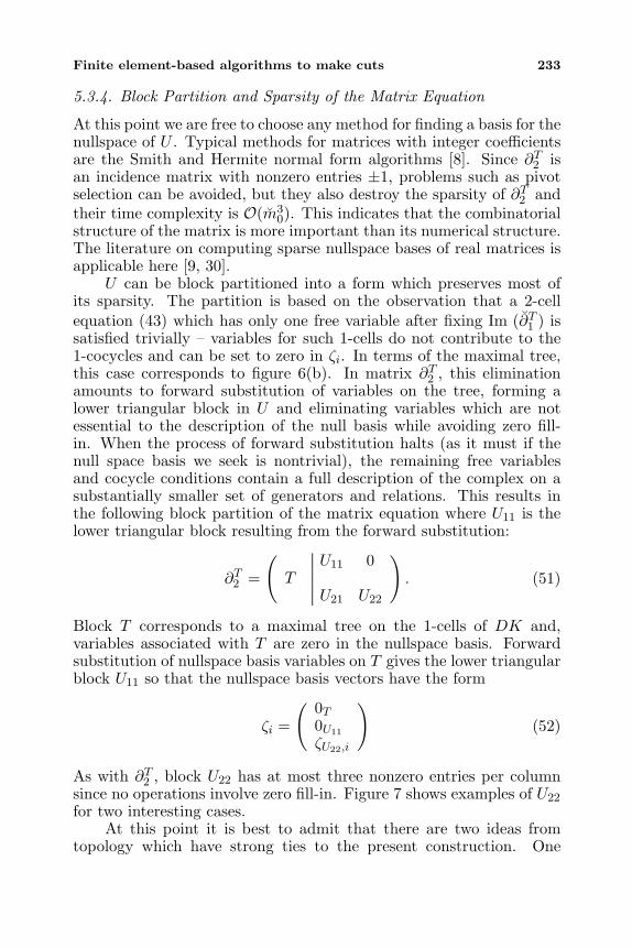
Finite element-based algorithms to make cuts 233
5.3.4. Block Partition and Sparsity of the Matrix Equation
At this point we are free to choose any method for finding a basis for thenullspace of U . Typical methods for matrices with integer coefficientsare the Smith and Hermite normal form algorithms [8]. Since ∂T2 isan incidence matrix with nonzero entries ±1, problems such as pivotselection can be avoided, but they also destroy the sparsity of ∂T2 andtheir time complexity is O(m3
0). This indicates that the combinatorialstructure of the matrix is more important than its numerical structure.The literature on computing sparse nullspace bases of real matrices isapplicable here [9, 30].
U can be block partitioned into a form which preserves most ofits sparsity. The partition is based on the observation that a 2-cellequation (43) which has only one free variable after fixing Im (∂T1 ) issatisfied trivially – variables for such 1-cells do not contribute to the1-cocycles and can be set to zero in ζi. In terms of the maximal tree,this case corresponds to figure 6(b). In matrix ∂T2 , this eliminationamounts to forward substitution of variables on the tree, forming alower triangular block in U and eliminating variables which are notessential to the description of the null basis while avoiding zero fill-in. When the process of forward substitution halts (as it must if thenull space basis we seek is nontrivial), the remaining free variablesand cocycle conditions contain a full description of the complex on asubstantially smaller set of generators and relations. This results inthe following block partition of the matrix equation where U11 is thelower triangular block resulting from the forward substitution:
∂T2 =
(U11 0
TU21 U22
). (51)
Block T corresponds to a maximal tree on the 1-cells of DK and,variables associated with T are zero in the nullspace basis. Forwardsubstitution of nullspace basis variables on T gives the lower triangularblock U11 so that the nullspace basis vectors have the form
ζi =
( 0T0U11
ζU22,i
)(52)
As with ∂T2 , block U22 has at most three nonzero entries per columnsince no operations involve zero fill-in. Figure 7 shows examples of U22
for two interesting cases.At this point it is best to admit that there are two ideas from
topology which have strong ties to the present construction. One
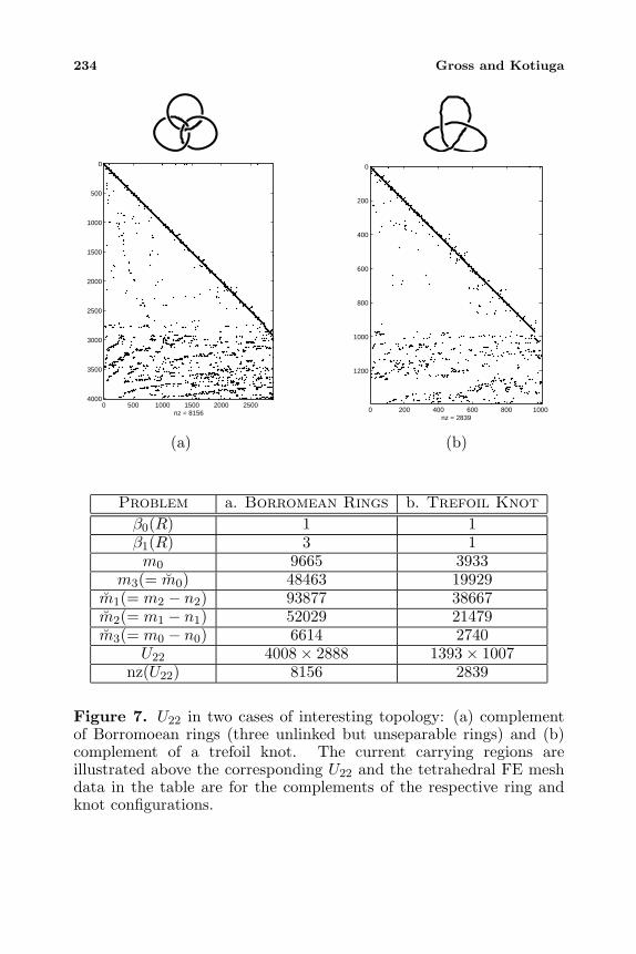
234 Gross and Kotiuga
0 500 1000 1500 2000 2500
0
500
1000
1500
2000
2500
3000
3500
4000
nz = 8156 0 200 400 600 800 1000
0
200
400
600
800
1000
1200
nz = 2839
(a) (b)
Problem a. Borromean Rings b. Trefoil Knot
β0(R) 1 1β1(R) 3 1m0 9665 3933
m3(= m0) 48463 19929m1(= m2 − n2) 93877 38667m2(= m1 − n1) 52029 21479m3(= m0 − n0) 6614 2740
U22 4008× 2888 1393× 1007nz(U22) 8156 2839
Figure 7. U22 in two cases of interesting topology: (a) complementof Borromoean rings (three unlinked but unseparable rings) and (b)complement of a trefoil knot. The current carrying regions areillustrated above the corresponding U22 and the tetrahedral FE meshdata in the table are for the complements of the respective ring andknot configurations.
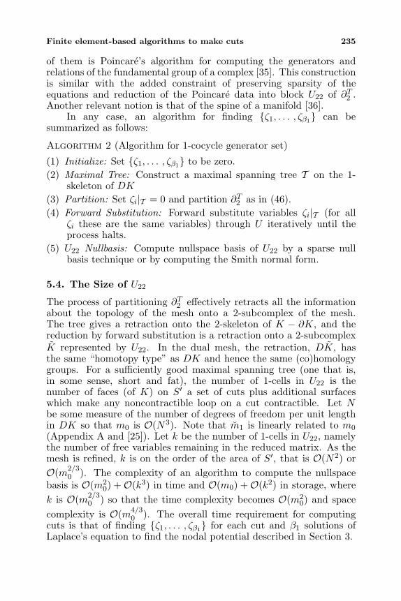
Finite element-based algorithms to make cuts 235
of them is Poincare’s algorithm for computing the generators andrelations of the fundamental group of a complex [35]. This constructionis similar with the added constraint of preserving sparsity of theequations and reduction of the Poincare data into block U22 of ∂T2 .Another relevant notion is that of the spine of a manifold [36].
In any case, an algorithm for finding ζ1, . . . , ζβ1 can besummarized as follows:
Algorithm 2 (Algorithm for 1-cocycle generator set)
(1) Initialize: Set ζ1, . . . , ζβ1 to be zero.(2) Maximal Tree: Construct a maximal spanning tree T on the 1-
skeleton of DK
(3) Partition: Set ζi|T = 0 and partition ∂T2 as in (46).(4) Forward Substitution: Forward substitute variables ζi|T (for all
ζi these are the same variables) through U iteratively until theprocess halts.
(5) U22 Nullbasis: Compute nullspace basis of U22 by a sparse nullbasis technique or by computing the Smith normal form.
5.4. The Size of U22
The process of partitioning ∂T2 effectively retracts all the informationabout the topology of the mesh onto a 2-subcomplex of the mesh.The tree gives a retraction onto the 2-skeleton of K − ∂K, and thereduction by forward substitution is a retraction onto a 2-subcomplexK represented by U22. In the dual mesh, the retraction, DK, hasthe same “homotopy type” as DK and hence the same (co)homologygroups. For a sufficiently good maximal spanning tree (one that is,in some sense, short and fat), the number of 1-cells in U22 is thenumber of faces (of K) on S′ a set of cuts plus additional surfaceswhich make any noncontractible loop on a cut contractible. Let Nbe some measure of the number of degrees of freedom per unit lengthin DK so that m0 is O(N3). Note that m1 is linearly related to m0
(Appendix A and [25]). Let k be the number of 1-cells in U22, namelythe number of free variables remaining in the reduced matrix. As themesh is refined, k is on the order of the area of S′, that is O(N2) orO(m2/3
0 ). The complexity of an algorithm to compute the nullspacebasis is O(m2
0) +O(k3) in time and O(m0) +O(k2) in storage, wherek is O(m2/3
0 ) so that the time complexity becomes O(m20) and space
complexity is O(m4/30 ). The overall time requirement for computing
cuts is that of finding ζ1, . . . , ζβ1 for each cut and β1 solutions ofLaplace’s equation to find the nodal potential described in Section 3.
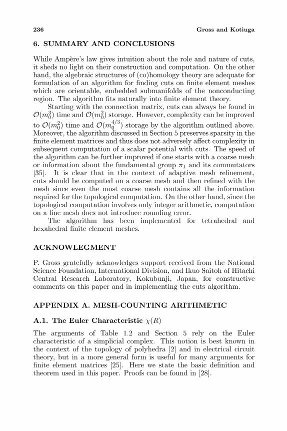
236 Gross and Kotiuga
6. SUMMARY AND CONCLUSIONS
While Ampere’s law gives intuition about the role and nature of cuts,it sheds no light on their construction and computation. On the otherhand, the algebraic structures of (co)homology theory are adequate forformulation of an algorithm for finding cuts on finite element mesheswhich are orientable, embedded submanifolds of the nonconductingregion. The algorithm fits naturally into finite element theory.
Starting with the connection matrix, cuts can always be found inO(m3
0) time and O(m20) storage. However, complexity can be improved
to O(m20) time and O(m4/3
0 ) storage by the algorithm outlined above.Moreover, the algorithm discussed in Section 5 preserves sparsity in thefinite element matrices and thus does not adversely affect complexity insubsequent computation of a scalar potential with cuts. The speed ofthe algorithm can be further improved if one starts with a coarse meshor information about the fundamental group π1 and its commutators[35]. It is clear that in the context of adaptive mesh refinement,cuts should be computed on a coarse mesh and then refined with themesh since even the most coarse mesh contains all the informationrequired for the topological computation. On the other hand, since thetopological computation involves only integer arithmetic, computationon a fine mesh does not introduce rounding error.
The algorithm has been implemented for tetrahedral andhexahedral finite element meshes.
ACKNOWLEGMENT
P. Gross gratefully acknowledges support received from the NationalScience Foundation, International Division, and Ikuo Saitoh of HitachiCentral Research Laboratory, Kokubunji, Japan, for constructivecomments on this paper and in implementing the cuts algorithm.
APPENDIX A. MESH-COUNTING ARITHMETIC
A.1. The Euler Characteristic χ(R)
The arguments of Table 1.2 and Section 5 rely on the Eulercharacteristic of a simplicial complex. This notion is best known inthe context of the topology of polyhedra [2] and in electrical circuittheory, but in a more general form is useful for many arguments forfinite element matrices [25]. Here we state the basic definition andtheorem used in this paper. Proofs can be found in [28].
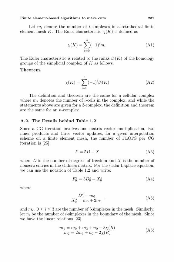
Finite element-based algorithms to make cuts 237
Let mi denote the number of i-simplexes in a tetrahedral finiteelement mesh K. The Euler characteristic χ(K) is defined as
χ(K) =3∑i=0
(−1)imi. (A1)
The Euler characteristic is related to the ranks βi(K) of the homologygroups of the simplicial complex of K as follows.
Theorem.
χ(K) =3∑i=0
(−1)iβi(K) (A2)
The definition and theorem are the same for a cellular complexwhere mi denotes the number of i-cells in the complex, and while thestatements above are given for a 3-complex, the definition and theoremare the same for an n-complex.
A.2. The Details behind Table 1.2
Since a CG iteration involves one matrix-vector multiplication, twoinner products and three vector updates, for a given interpolationscheme on a finite element mesh, the number of FLOPS per CGiteration is [25]
F = 5D + X (A3)
where D is the number of degrees of freedom and X is the number ofnonzero entries in the stiffness matrix. For the scalar Laplace equation,we can use the notation of Table 1.2 and write:
F s0 = 5Ds
0 + Xs0 (A4)
where
Ds0 = m0
Xs0 = m0 + 2m1
. (A5)
and mi, 0 ≤ i ≤ 3 are the number of i-simplexes in the mesh. Similarly,let ni be the number of i-simplexes in the boundary of the mesh. Sincewe have the linear relations [23]
m1 = m0 + m3 + n0 − 3χ(R)m2 = 2m3 + n0 − 2χ(R) (A6)
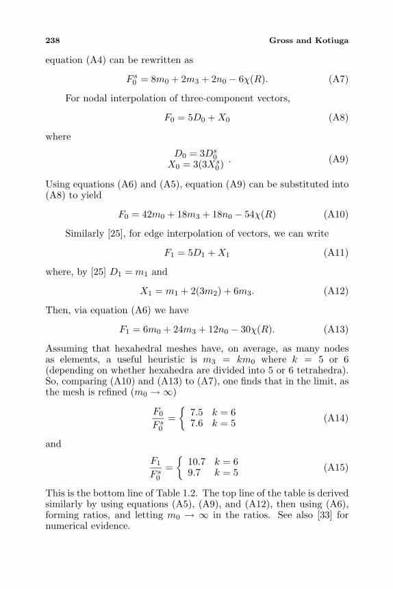
238 Gross and Kotiuga
equation (A4) can be rewritten as
F s0 = 8m0 + 2m3 + 2n0 − 6χ(R). (A7)
For nodal interpolation of three-component vectors,
F0 = 5D0 + X0 (A8)
where
D0 = 3Ds0
X0 = 3(3Xs0) . (A9)
Using equations (A6) and (A5), equation (A9) can be substituted into(A8) to yield
F0 = 42m0 + 18m3 + 18n0 − 54χ(R) (A10)
Similarly [25], for edge interpolation of vectors, we can write
F1 = 5D1 + X1 (A11)
where, by [25] D1 = m1 and
X1 = m1 + 2(3m2) + 6m3. (A12)
Then, via equation (A6) we have
F1 = 6m0 + 24m3 + 12n0 − 30χ(R). (A13)
Assuming that hexahedral meshes have, on average, as many nodesas elements, a useful heuristic is m3 = km0 where k = 5 or 6(depending on whether hexahedra are divided into 5 or 6 tetrahedra).So, comparing (A10) and (A13) to (A7), one finds that in the limit, asthe mesh is refined (m0 →∞)
F0
F s0
=
7.5 k = 67.6 k = 5 (A14)
and
F1
F s0
=
10.7 k = 69.7 k = 5 (A15)
This is the bottom line of Table 1.2. The top line of the table is derivedsimilarly by using equations (A5), (A9), and (A12), then using (A6),forming ratios, and letting m0 → ∞ in the ratios. See also [33] fornumerical evidence.
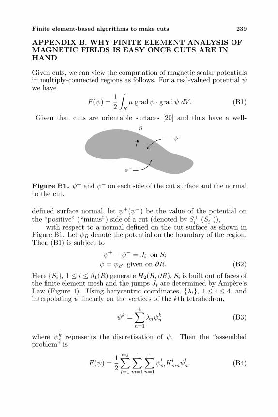
Finite element-based algorithms to make cuts 239
APPENDIX B. WHY FINITE ELEMENT ANALYSIS OFMAGNETIC FIELDS IS EASY ONCE CUTS ARE INHAND
Given cuts, we can view the computation of magnetic scalar potentialsin multiply-connected regions as follows. For a real-valued potential ψwe have
F (ψ) =12
∫Rµ gradψ · gradψ dV. (B1)
Given that cuts are orientable surfaces [20] and thus have a well-
ψ−
n
ψ+
Figure B1. ψ+ and ψ− on each side of the cut surface and the normalto the cut.
defined surface normal, let ψ+(ψ−) be the value of the potential onthe “positive” (“minus”) side of a cut (denoted by S+
i (S−i )),with respect to a normal defined on the cut surface as shown in
Figure B1. Let ψB denote the potential on the boundary of the region.Then (B1) is subject to
ψ+ − ψ− = Ji on Siψ = ψB given on ∂R. (B2)
Here Si, 1 ≤ i ≤ β1(R) generate H2(R, ∂R), Si is built out of faces ofthe finite element mesh and the jumps Ji are determined by Ampere’sLaw (Figure 1). Using barycentric coordinates, λi, 1 ≤ i ≤ 4, andinterpolating ψ linearly on the vertices of the kth tetrahedron,
ψk =4∑
n=1
λnψkn (B3)
where ψkn represents the discretisation of ψ. Then the “assembledproblem” is
F (ψ) =12
m3∑l=1
4∑m=1
4∑n=1
ψlmKlmnψ
ln. (B4)
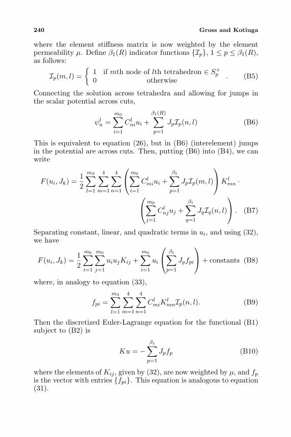
240 Gross and Kotiuga
where the element stiffness matrix is now weighted by the elementpermeability µ. Define β1(R) indicator functions Ip, 1 ≤ p ≤ β1(R),as follows:
Ip(m, l) =
1 if mth node of lth tetrahedron ∈ S+p
0 otherwise . (B5)
Connecting the solution across tetrahedra and allowing for jumps inthe scalar potential across cuts,
ψln =m0∑i=1
C lniui +
β1(R)∑p=1
JpIp(n, l) (B6)
This is equivalent to equation (26), but in (B6) (interelement) jumpsin the potential are across cuts. Then, putting (B6) into (B4), we canwrite
F (ui, Jk) =12
m3∑l=1
4∑m=1
4∑n=1
m0∑i=1
C lmiui +
β1∑p=1
JpIp(m, l)
K l
mn ·
m0∑j=1
C lnjuj +
β1∑q=1
JqIq(n, l)
. (B7)
Separating constant, linear, and quadratic terms in ui, and using (32),we have
F (ui, Jk) =12
m0∑i=1
m0∑j=1
uiujKij +m0∑i=1
ui
β1∑p=1
Jpfpi
+ constants (B8)
where, in analogy to equation (33),
fpi =m3∑l=1
4∑m=1
4∑n=1
C lmiK
lmnIp(n, l). (B9)
Then the discretized Euler-Lagrange equation for the functional (B1)subject to (B2) is
Ku = −β1∑p=1
Jpfp (B10)
where the elements of Kij , given by (32), are now weighted by µ, and fpis the vector with entries fpi. This equation is analogous to equation(31).
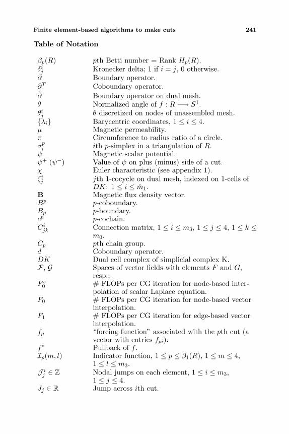
Finite element-based algorithms to make cuts 241
Table of Notation
βp(R) pth Betti number = Rank Hp(R).δij Kronecker delta; 1 if i = j, 0 otherwise.∂ Boundary operator.∂T Coboundary operator.∂ Boundary operator on dual mesh.θ Normalized angle of f : R −→ S1.θij θ discretized on nodes of unassembled mesh.λi Barycentric coordinates, 1 ≤ i ≤ 4.µ Magnetic permeability.π Circumference to radius ratio of a circle.σpi ith p-simplex in a triangulation of R.ψ Magnetic scalar potential.ψ+ (ψ−) Value of ψ on plus (minus) side of a cut.χ Euler characteristic (see appendix 1).ζij jth 1-cocycle on dual mesh, indexed on 1-cells of
DK: 1 ≤ i ≤ m1.B Magnetic flux density vector.Bp p-coboundary.Bp p-boundary.cp p-cochain.Cijk Connection matrix, 1 ≤ i ≤ m3, 1 ≤ j ≤ 4, 1 ≤ k ≤
m0.Cp pth chain group.d Coboundary operator.DK Dual cell complex of simplicial complex K.F , G Spaces of vector fields with elements F and G,
resp..F s
0 # FLOPs per CG iteration for node-based inter-polation of scalar Laplace equation.
F0 # FLOPs per CG iteration for node-based vectorinterpolation.
F1 # FLOPs per CG iteration for edge-based vectorinterpolation.
fp “forcing function” associated with the pth cut (avector with entries fpi).
f∗ Pullback of f .Ip(m, l) Indicator function, 1 ≤ p ≤ β1(R), 1 ≤ m ≤ 4,
1 ≤ l ≤ m3.J ij ∈ Z Nodal jumps on each element, 1 ≤ i ≤ m3,
1 ≤ j ≤ 4.Jj ∈ R Jump across ith cut.

242 Gross and Kotiuga
H Magnetic field intensity.Hp(R;Z) pth cohomology group of R with coefficients in Z.Hp(R;Z) pth homology group of R, coefficients in Z.Hp(R, ∂R;Z) pth cohomology group of R relative to ∂R, coeffi-
cients in Z.Hp(R, ∂R;Z) pth homology group of R relative to ∂R, coeffi-
cients in Z.K Simplicial complex.Kkmn Stiffness matrix, 1 ≤ m,n ≤ 4, 1 ≤ k ≤ m3.
mp Number of p-simplexes in a triangulation of R.mp Number of p-cells in dual complex.np Number of p-simplexes in a triangulation of ∂R.O(nα) Order nα.P Period matrix, equation (21).R Region in R3, free of conduction currents, where
the field is sought.S Surface.Sq qth cut.S1 Unit circle, S1 = p ∈ C | |p| = 1.uk Nodal potential, 1 ≤ k ≤ m0.Xs
0 # nonzero entries in stiffness matrix for node-basedscalar interpolation.
X0 # nonzero entries in stiffness matrix for node-basedvector interpolation.
X1 # nonzero entries in stiffness matrix for edge-basedvector interpolation.
z Complex conjugate of z.zp p-cocycle.zp p-cycle.[A,B] Homotopy classes of maps f : A→ B.
REFERENCES
1. Adkins, W. A. and S. H. Weintraub, Algebra: An Approach viaModule Theory, 307–327, Springer-Verlag, New York, 1992.
2. Armstrong, M., Basic Topology, Springer-Verlag, New York, 1983.3. Balabanian, N. and T. A. Bickart, Electrical Network Theory, 80,
John Wiley and Sons, New York, 1969.4. Bamberg, P. and S. Sternberg, A Course in Mathematics for
Students of Physics: 2, Ch. 12, Cambridge U. Press, NY, 1990.5. Bossavit, A., A. Vourdas, and K. J. Binns, “Magnetostatics with
scalar potentials in multiply connected regions,” IEE Proc. A,
Finite element-based algorithms to make cuts 243
Vol. 136, 260–261, 1989.6. Bott, R. and L. W. Tu, Differential Forms in Algebraic Topology,
40–42, 51, 234, 258, 240, Springer-Verlag, New York, 1982.7. Brown, M. L., “Scalar potentials in multiply connected regions,”
Int. J. Numer. Meth. Eng., Vol. 20, 665–680, 1984.8. Cohen, H., A Course in Computational Algebraic Number Theory,
Springer-Verlag, New York, 1993.9. Coleman, T. F., A. Edenbrandt, and J. R. Gilbert, “Predicting fill
for sparse orthogonal factorization,” Journal of the Association forComputing Machinery, Vol. 33, 517–532, 1986.
10. Croom, F. H., Basic Concepts of Algebraic Topology, Chaps. 2,7.3, 4.5, Springer-Verlag, New York, 1978.
11. Deschamps, G. A., “Electromagnetics and differential forms,”IEEE Proc., Vol. 69, 676–696, 1981.
12. Greenberg, M. J. and J. R. Harper, Algebraic Topology, 235, 63–66Benjamin/Cummings, Reading, MA, 1981.
13. Gross, P. W., “The commutator subgroup of the first homotopygroup and cuts for scalar potentials in multiply connectedregions,” Master’s thesis, Dept. of Biomed. Eng., Boston U.,September 1993.
14. Gross, P. W. and P. R. Kotiuga, “Data structures for geometricand topological aspects of finite element algorithms,” this volume.
15. Gross, P. W. and P. R. Kotiuga, “A challenge for magneticscalar potential formulations of 3-d eddy current problems:Multiply connected cuts in multiply connected regions whichnecessarily leave the cut complement multiply connected,” Electricand Magnetic Fields: From Numerical Models to IndustrialApplications, A. Nicolet and R. Belmans (eds.), Plenum, 1–20,New York, 1995. Proc. of the Second Int. Workshop on Electricand Magnetic Fields.
16. Guillemin, V. and A. Pollack, Differential Topology, 21, Prentice-Hall, Englewood Cliffs, New Jersey, 1974.
17. Gunning, R. C. and H. Rossi, Analytic Functions of SeveralComplex Variables, Prentice-Hall, Englewood Cliffs, N.J., 1965.
18. Harrold, C. S. and J. Simkin, “Cutting multiply connecteddomains,” IEEE Trans. Magn., Vol. 21, 2495–2498, 1985.
19. Kotiuga, P. R., “Hodge decompositions and computationalelectromagnetics,” Ph.D. thesis, McGill University, Montreal,1984.
20. Kotiuga, P. R., “On making cuts for magnetic scalar potentials inmultiply connected regions,” J. Appl. Phys., Vol. 61, 3916–3918,
244 Gross and Kotiuga
1987.21. Kotiuga, P. R., “An algorithm to make cuts for scalar potentials
in tetrahedral meshes based on the finite element method,” IEEETrans. Magn., Vol. 25, 4129–4131, 1989.
22. Kotiuga, P. R., “Topological considerations in coupling scalarpotentials to stream functions describing surface currents,” IEEETrans. Magn., Vol. 25, 2925–2927, 1989.
23. Kotiuga, P. R., “Analysis of finite-element matrices arising fromdiscretizations of helicity functionals,” J. Appl. Phys., Vol. 67,5815–5817, 1990.
24. Kotiuga, P. R., “Topological duality in three-dimensional eddy-current problems and its role in computer-aided problemformulation,” J. Appl. Phys., Vol. 67, 4717–4719, 1990.
25. Kotiuga, P. R., “Essential arithmetic for evaluating threedimensional vector finite element interpolation schemes,” IEEETrans. Magn., Vol. 27, 5208–5210, 1991.
26. Kotiuga, P. R., A. Vourdas, and K. J. Binns, “Magnetostaticswith scalar potentials in multiply connected regions,” IEE Proc.A, Vol. 137, 231–232, 1990.
27. Maxwell, J. C., A Treatise on Electricity and Magnetism (1891),Chap. 1, Art. 18–22, Dover, New York, 1954.
28. Munkres, J. R., Elements of Algebraic Topology, 377–380,Addison-Wesley, Reading, MA, 1984.
29. Murphy, A., “Implementation of a finite element based algorithmto make cuts for magnetic scalar potentials,” Master’s thesis,Dept. of ECS Eng., Boston U., 1991.
30. Pothen, A. and C.-J. Fan, “Computing the block triangular formof a sparse matrix,” ACM Transactions on Mathematical Software,Vol. 16, 303–324, 1990.
31. Ren, Z. and A. Razek, “Boundary edge elements andspanning tree technique in three-dimensional electromagnetic fieldcomputation,” Int. J. Num. Meth. Eng., Vol. 36, 2877–2893, 1993.
32. Rotman, J. J., An Introduction to Algebraic Topology, Springer-Verlag, NY, 1988.
33. Saitoh, I., “Perturbed H-method without the Lagrange multiplierfor three dimensional nonlinear magnetostatic problems,” IEEETrans. Magn., Vol. 30, 4302–4304, 1994.
34. Silvester, P. and R. Ferrari, Finite Elements for ElectricalEngineers, 2nd Edition, Cambridge U. Press, NY, 1990.
35. Stillwell, J., Classical Topology and Combinatorial Group Theory,Second Edition, Ch. 3,4, Springer-Verlag, NY, 1993.

Finite element-based algorithms to make cuts 245
36. Thurston, W. P., Three-Dimensional Geometry and Topology,Princeton University Press, Princeton, New Jersey, 1997.
37. Vourdas, A. and K. J. Binns, “Magnetostatics with scalarpotentials in multiply connected regions,” IEE Proc. A, Vol. 136,49–54, 1989.
Progress In Electromagnetics Research, PIER 32, 247–269, 2001
DISCRETE HODGE-OPERATORS: AN ALGEBRAICPERSPECTIVE
R. Hiptmair
Sonderforschungsbereich 382Universitat Tubingen72076 Tubingen, Germany
Abstract—Discrete differential forms should be used to deal with thediscretization of boundary value problems that can be stated in thecalculus of differential forms. This approach preserves the topologicalfeatures of the equations. Yet, the discrete counterparts of the metric-dependent constitutive laws remain elusive.
I introduce a few purely algebraic constraints that matricesassociated with discrete material laws have to satisfy. It turns outthat most finite element and finite volume schemes comply with theserequirements. Thus convergence analysis can be conducted in a unifiedsetting. This discloses basic sufficient conditions that discrete materiallaws have to meet in order to ensure convergence in the relevant energynorms.
1 Introduction
2 Discrete Differential Forms
3 Discrete Hodge Operators
4 Examples
5 Abstract Error Analysis
6 Estimation of Consistency Errors
References
1. INTRODUCTION
The focus of this paper is on linear stationary boundary value problemsthat can be expressed in the calculus of differential forms (For
248 Hiptmair
introduction/survey see [19, 33, 9, 10]). Let Ω ⊂ Rn, n ∈ N, be somedomain, whose (piecewise smooth) boundary ∂Ω is partitioned intoΓD, ΓN , and ΓM . The generic boundary value problem stated in thelanguage of differential forms is given by
d u = (−1)lσ , d j = −ψ + φtDu = 0 on ΓD , tN j = 0 on ΓN
j = α σ , ψ = γ u in Ω
tM j = (−1)l−1 Γβ tMu on ΓM .
Here, d is the exterior derivative of exterior calculus, and u, σ, j, ψ,and φ are differential forms of different orders. More precisely, if u isan l − 1-form, l ∈ N, then σ is an l-form, j an m-form, m := n − l,whereas both ψ and φ are of order m+ 1. In (1), φ can be regarded assource term, while we have to solve for the other forms u, σ, j, and ψ.Of course, knowledge of u is sufficient.
The linear operators tD, tN , and tM stand for the trace ofdifferential forms onto ΓD, ΓN , and ΓM , respectively [33, Sect. 1.10].They preserve the order of the form and commute with exteriordifferentiation.
We pay special attention to the Hodge-operators γ and β. Theysupply linear mappings of (continuous) l-forms into n − l-forms. Incontrast to most other concepts in the theory of differential forms,Hodge-operators are not meaningful on their own, but they have tobe spawned by Riemannian metrices. For the details I refer to [33,Sect. 1.4] or [7, Sect. 4.5]. Therefore, in (1) α, γ and β designateuniformly positive metrices on Ω and ΓM , respectively.
Translated into vector calculus (1) covers a wide array of boundaryvalue problems. For instance, in three dimensions we recover standardsecond order elliptic boundary value problems in the case l = 1.Boundary value problems involving the double -curl-operator thatarise in quasistatic electromagnetism are included as the case l = 2.
The formulation (1) is often dismissed as nice but moot, becausepeople doubt whether the perspective of differential forms brings anytangible gains. The main message I want to send in this paper is thatthere is a substantial benefit both for the design, understanding, anderror analysis of discretization procedures. I am by no means the first tomake this point. I would like to mention Matiussi [35], Tonti [49], Dezin[24], Shashkov [30, 32], Chew [20, 48], and, most prominently, Bossavit[5, 8, 9, 7, 4, 3, 47]. Whereas the foundation is borrowed from theseworks, I am setting out to build upon it a general unifying frameworkfor the quantitative analysis of a wide class of finite element andfinite volume schemes. In a sense, the present paper supplements the
Discrete Hodge-operators 249
previous conceptual works by what is cherished as “rigorous analysis”and “abstract treatment”. The reader can view it as an extension ofA. Bossavit’s paper [13], in which the concepts are exposed for theconcrete case of Maxwell’s equations. The benefit of abstraction is thatfundamental relationships between different discretization schemes willbe disclosed, widening the scope of techniques originally developed foronly one type of method.
One insight can already be gleaned from (1). It is obvious thatthe top line in (1) and the boundary conditions on ΓD and ΓN donot involve any metric. They represent the topological relationshipsunderlying the boundary value problems. I will refer to them asequilibrium equations (topological field equations in [48]). On top ofthat the two equilibrium equations are not directly coupled. Onemay view them as equations for different kinds of differential forms:“ordinary” forms and twisted forms [18, 7, 48, 13]. The link betweenthe equilibrium equations is established by the constitutive relations(material laws, metric field equations [48]) that essentially depend onmetrics.
Admittedly, there is a price tag on generality. The results I amgetting may be weaker than those obtained through more specializedtechniques. In addition, quite a few cumbersome details may still beleft to work out for specific schemes. However, the sheer scope of themethod compensates for these drawbacks. It can also serve as a reliableguide to the construction of appropriate schemes.
The paper is organized as follows: The next section reviewsdiscrete differential forms, i.e., finite elements for differential forms.The third section introduces the key concept of discrete Hodge-operators and gives a purely algebraic characterization. Similar, thoughmore restricted, approaches to the construction of discrete Hodgeoperators are pursued in [47] and [48, Sect. VII]. The fourth sectionstudies examples of discrete Hodge operators. In particular, the focus ison finite volume methods. Using only a few basic algebraic propertiesof discrete Hodge operators, abstract bounds for the energies of thediscretization errors are established in the fifth section. This is furtherelaborated in the case of concrete schemes in the sixth section.
2. DISCRETE DIFFERENTIAL FORMS
When solving (1) numerically, we hope to get a good approximationof all or some of the unknown differential forms that can be describedby a finite number of real numbers. It is reasonable to insist that thisapproximation is a valid differential form itself. In short, as result ofthe computation we expect to get a discrete differential form.
250 Hiptmair
Definition 2.1 A sequence of spaces W l, 0 ≤ l ≤ n, providesdiscrete differential forms on Ω, if
• the integral of any ω ∈ W l over any piecewise smooth l-dimensional oriented manifold is well defined.
• dW l ⊂ W l+1 for 0 ≤ l < n.• all the spaces W l have finite dimension.• there is a linear mapping I lh from l-forms onto W l satisfying the
commuting diagram property dI lhω = I l+1h (dω) for all l-forms ω,
0 ≤ l < n (see e.g. [47, Sect. IV]).
In the sequel I take for granted that the corresponding discretedifferential forms comply with the boundary traces tN j = 0 andtDu = 0 stated in (1).
In practice, the W l are constructed as finite element spaces. Inparticular, the discrete differential forms are usually built upon somemesh (tessellation, cell complex) of Ω (cf. [48, Sect. IV])
Definition 2.2 For any 0 ≤ k ≤ n denote by Fk a collectionof piecewise smooth oriented contractible k-dimensional submanifolds(k-facets) of Ω such that
• for distinct facets their interiors are disjoint regardless ofdimension.
• the intersection of the closures of any two facets of any dimensionscoincides with the closure of one and only one other facet.
• the boundary of each k-facet, 1 ≤ k ≤ n, is the union of a finitenumber of k + 1-facets.
• the union of the closures of all n-facets is equal to Ω.
Then Fknk=0 forms a mesh Th of Ω, and Fn is the set of its cells.The boundary parts ΓN , ΓD, and ΓM are to be composed of
entire faces of elements. Thus, by plain restriction of a mesh of Ωwe get meshes of ΓN , ΓD, and ΓM . By dropping all facets containedin the closure of ΓD (ΓN ) we end up with the so-called ΓD(ΓN )-active mesh. Examples of valid meshes are the customary finite elementtriangulations in the sense of [21].
For discrete differential forms on triangulations the first conditionstated in definition (2.1) is equivalent to demanding that the traces ofthe discrete l-form on any k-dimensional facet, l ≤ k ≤ n have to bewell defined [27].
In the sequel we only consider (generalized) Whitney-forms, i.e.discrete differential l-forms, whose degrees of freedom are supplied byintegrals over l-facets of the mesh. Mainly for the sake of simplicity,because the basic considerations carry over to higher order elements, as
Discrete Hodge-operators 251
well. However, we admit rather general meshes according to definition(2.2). The only restriction should be that any cell can be split into afew (curved) simplices. Hence, for complicated shapes of elements wecan come up with composite Whitney-elements.
For each space W l we pick the basis dual to the set of degreesof freedom and assume a numbering of the basis functions. Thus, adifferential form uh ∈ W l is uniquely characterized by its coefficientvector u ∈ Cl, where we have abbreviated Cl := R
Nl , Nl := dimW l
(number of active l-facets). I tag coefficient vectors by and discretedifferential forms by a subscript h. The latter can also be seen as amapping assigning a differential form in W l to some coefficient vector∈ Cl. This induces a matrix representation for all linear operators onthe spaces W l, l = 0, . . . , n. For instance, we write Dl ∈ RNl+1×Nlfor the matrix representing the exterior derivative d : W l → W l+1.These matrices turn out to be the incidence matrices of the activemesh [5, 39, 41, 11], e.g., Dl is the incidence matrix of oriented activel-facets and active l+1-facets. Both from this background and dd = 0we can conclude DlDl−1 = 0, l = 1, . . . , n [5, Ch. 5].
It goes without saying that the trace operators tD, tN , and tMpossess matrix representations, too. Those are particularly simple,because taking the trace of a discrete differential form on a part ofthe boundary just amounts to isolating the d.o.f. located there [27].We chose the symbol T for these matrices.
Now, we are already able to come up with the discrete equilibriumequations
Dl−1u = (−1)lσ , Dmj = −ψ + φ . (1)
Here, φ is the coefficient vector of some suitable interpolant ∈ Wm+1
of the source term φ. The reader should be aware that whateverfeatures of the equations arise from the equilibrium equations aloneare preserved in the discrete setting. For instance, for any orientedcontrol volume Ω′ ⊂ Ω∫
Ω′
(σh ∧ jh + uh ∧ ψh) =∫Ω′
uh ∧ φh + (−1)l∫∂Ω′
σh ∧ jh .
In short, thanks to discrete differential forms we automatically achievediscrete models that inherit most of the global features of the originalproblem (cf. [34, 20] for a discussion of Maxwell’s equations and [32]for discrete decomposition theorems).
Remark. The discrete equilibrium equations (1) could also havebeen derived as network or lattice equations [11, 20, 52, 15] by applyingStokes’ theorem directly to facets of the mesh in the spirit of a finite
252 Hiptmair
volume approach. Yet, my point is that discrete differential formsare indispensable when trying to assess the approximation propertiesof discretization schemes. This will be elucidated in the remainingsections.
3. DISCRETE HODGE OPERATORS
The Hodge operators defy a straightforward discretization in thespaces of discrete differential forms: Consider the example of adiscrete 1-form ω in three dimensions (“edge elements”): Its vectorrepresentative u sports only tangential continuity [38] and so itsnormal components on interelement faces are not necessarily welldefined. The Hodge operator belonging to the Euclidean metric leavesvector representatives unchanged, i.e. the (twisted) 2-form ω is alsodescribed by u. If F is a face, at which the normal component of u has ajump, it is not possible to evaluate the integral
∫F ω =
∫F 〈u,nF 〉 dS:
This reveals that ω fails to supply a proper discrete 2-form on thesame mesh.
Thus, when embracing discrete differential forms, one inevitablystumbles onto the issue of a discrete Hodge operator [47, 34, 23, 12].Its construction is outside the scope of the canonical discrete exteriorcalculus, because the standard definition of the Hodge operator isa “strong concept”, which relies on point values being well defined.However, conventional discrete differential forms, with the exceptionof discrete 0-forms, are inherently discontinuous at interelement faces.This situation is typical of finite element methods: Recall piecewiselinear finite element whose derivative is also meaningless in a pointwisesense. We are forced to resort to “weak concepts” that involvevariational principles. This is not a nuisance, but leaves us with amplechoices (cf. the introduction of [11]).
One aspect of this freedom arises from the observation that thetwo equilibrium equations are only linked through the constitutiverelations. In fact, they involve differential forms of different nature(ordinary and twisted). So there is no reason, why both equilibriumequations should be discretized via the same family of discretedifferential forms:
In general, the two equilibrium equations can be discretized ondifferent unrelated meshes of Ω, called primary mesh Th and secondarymesh Th.
I stress that absolutely no relationship between these two meshesis stipulated. The terms “primary” and “secondary” must not eveninsinuate some precedence. I adopt the convention that all symbolsrelated to the secondary mesh will be labeled by a tilde. This applies
Discrete Hodge-operators 253
to matrices acting on coefficient vectors of discrete differential formson the secondary mesh, too.
Basically, discrete versions of the Hodge operators occurring in(1) have to establish linear mappings between spaces of discrete l-forms and n − l-forms based on possibly different meshes. In otherwords, a discrete Hodge-operators can be described by a Nm × Nl-matrix. Moreover, for continuous l-forms α 1/α = (−1)ln−l · Id [33,Sect. 1.8], i.e. the Hodge operators are invertible. This must hold fordiscrete Hodge-operators, too.
To get down to specifics, remember that Hodge operators defineinner products on space of continuous differential forms via (ω, η)α :=∫Ω ω ∧ α η. Here ∧ denotes the exterior product of differential forms,
which generates an l + k-form when given an l-form and a k-form asarguments. The exterior product is a bilinear mapping. Admittedly, theinner product (ω, η)α is of little value, because it would yield a circular“definition” of a discrete Hodge operator. Yet, the relationship revealsthe general pattern:
µw = ω
(−1)ln−l 1/µ ω = w
↔
(w, η)µ =∫Ω
ω ∧ η ∀ l-forms η
(−1)ln−l (ω, v)1/µ =∫Ω
w ∧ v∀ m-forms v .
(2)
This suggests the following generic discrete form for a material lawlinking an ordinary l-form w and a twisted m-form ω:
µw = ω
(−1)ln−l 1/µ ω = w
discretize−→
Mlµ w = Klmω
or(−1)ln−l Mm
1/µω = Kml w ,
(3)
with yet obscure matrices Mlµ, Mm
1/µ, and Kml , Klm. In an obviousfashion, the various indices are related to the order of differential formson whose coefficient vectors the matrices act. Note that the discreteversions of the equivalent continuous material laws need not remainequivalent as explained in [48, Sect. VII]: In general we must reckonwith
Mlµ · (−1)ln−l Mm
1/µ = ENm ,
254 Hiptmair
where ENm is the Nm × Nm identity matrix. An equality would bedesirable, but seems to be rather elusive, as we will see in a moment.In sum, we can distinguish between two versions of the same materiallaw. I dub the upper discrete material law “primary”, the lower“secondary”.
The matrices from (3) have to satisfy only a few algebraicrequirements:
The first states that both Mlµ ∈ RNl,Nl and Mm
1/µ ∈ RNm,Nm are to besquare, symmetric, and positive definite matrices, where Nl := dimW l,Nm := dim Wm. This is natural if they are to give rise to inner productsas explained above.
The second wants the “pairing matrices” Kml ∈ RNm,Nl and Klm ∈RNl,Nm to fulfill
Kml = (−1)lm(Klm)T ⇐⇒ Klm = (−1)lm(Kml )T (4)
for all 0 ≤ l,m ≤ n such that l +m = n. Keep in mind that Kml andKlm somehow approximate
∫Ω ω ∧ η and
∫Ωw ∧ v. Then the equation
ω ∧ η = (−1)lkη ∧ ω , ω l-form, η k-form (5)
immediately leads to (4).
The third requirement is the discrete counterpart of the integrationby parts formula [33, Sect. 3.2]∫
Ω
dω ∧ η + (−1)l∫Ω
ω ∧ dη =∫∂Ω
ω ∧ η (6)
for l-forms ω, k-forms η, 0 ≤ l, k < n − 1, l + k = n − 1. Here, theboundary ∂Ω is endowed with the induced orientation. In the discretesetting this means
(Dl−1u)T Klmv = (−1)l uT Kl−1m+1D
mv + (Tl−1Γ u)T Kl−1
m,ΓTmΓ v . (7)
for all u ∈ Cl−1, v ∈ Cm, and translates into
(Dl−1)T Klm = (−1)l Kl−1m+1D
m + (Tl−1Γ )T Kl−1
m,ΓTmΓ (8)
for all 0 < m, l < n with l+m = n. Here, we denote by Klm,Γ a pairingmatrix acting on degrees of freedom on the boundary part ΓM . Using(4), (8) can be converted into
(Dm)TKm+1l−1 = (−1)m+1Kml Dl−1 + (TmΓ )TKml−1,ΓTl−1
Γ . (9)
Discrete Hodge-operators 255
Let us assume that we have found a discrete Hodge operator accordingto the above specifications. Nevertheless, we cannot be sure that theresulting linear system of equation has a solution at all. Usually thenumber of unknowns and equations will not agree. To end up with asquare linear system of equations we eliminate some of the unknownsby means of (8), (9) and the material laws. I first consider (1) anddiscuss some variants of choosing the discrete Hodge operators. I startwith listing the formal discrete constitutive laws that might be used inthe discretization of (1):
Primary:
Mlασ = Klm
j (a)Ml−1γ u = Kl−1
m+1ψ (b)
Ml−1β,ΓTl−1
Γ u = (−1)l−1 Kl−1m,ΓTmΓ
j (c)
(10)
Secondary:
Mm1/αj = (−1)mn−m Kml σ (a)
Mm+11/γ
ψ = (−1)(l−1)(n−1) Km+1l−1 u (b)
Mm1/β,ΓTmΓ
j = (−1)(l−1)(n−1) Kml−1,ΓTl−1Γ u (c)
(11)
1. Primary elimination: Using only primary discrete Hodge operators(10a), (10c) and (1), (8) we get
(Dl−1)TMlαDl−1u = (Dl−1)T (−1)lMl
ασ = (−1)l(Dl−1)T Klmj =
= Kl−1m+1D
mj + (−1)l(Tl−1Γ )T Kl−1
m,ΓTmΓj =
= Kl−1m+1(−ψ + φ)− (Tl−1
Γ )TMl−1β,ΓTl−1
Γ u =
= −Ml−1γ u− (Tl−1
Γ )TMl−1β,ΓTl−1
Γ u+ Kl−1m+1
φ .
We arrive at a linear system of equations
(Dl−1)TMlαDl−1u+ Ml−1
γ u+ (Tl−1Γ )TMl−1
β,ΓTl−1Γ u = Kl−1
m+1φ (12)
for the unknown coefficients u with a symmetric positive definitecoefficient matrix. If γ = 0, it has a unique solution. Even if γ = 0,at least Dl−1u can be uniquely determined. Two more importantfacts have to mentioned: To begin with, the secondary spaces do onlyaffect the right hand side Kl−1
m+1φ of the final system. In other words,
the choice of the secondary mesh is totally irrelevant as regards theultimate system matrix. Secondly, in the process of elimination weirretrievable lost information about the secondary unknowns σh andψh, unless the pairing matrices are invertible.
256 Hiptmair
2. Secondary elimination: We exclusively rely on secondary discreteHodge operators (11b), (11c) along with (1), (9):
Mm1/αj = (−1)n(m+1)Kml Dl−1u
= (−1)(n−1)(l−1)((Dm)TKm+1l−1 u− (TmΓ )TKml−1,ΓTl−1
Γ u)
= (Dm)T Mm+11/γ
ψ − (TmΓ )T Mm1/β,ΓTmΓ
j
Introducing the auxiliary unknown ζ := Mm+11/γ
ψ we get the saddlepoint problem(
Mm1/α + (TmΓ )T Mm
1/β,ΓTmΓ −(Dm)T
−Dm −(Mm+11/γ )−1
)(jζ
)=
(0−φ
). (13)
As the diagonal blocks are positive and negative definite, respectively,this linear system has a unique solution (cf. [17]). In the case ofvanishing γ we just define the auxiliary unknown as ζ := Km+1
l−1 u andstill get uniqueness for j. Parallel to the purely primal case we observethat no trace of the primary discrete spaces is left. As above, in generalwe cannot solve for the primary unknowns u and σ.3. Hybrid elimination: Both primary and secondary discrete Hodgeoperators are used for the sake of eliminating unknowns. For example,if we use primary representations (10a), (10c) for the material lawsj = α σ and tM j = (−1)l−1 Γβ tMu, but the secondary version (11b)for ψ = γ u we get
(Dl−1)TMlαDl−1u+ (Tl−1
Γ )TMl−1β,ΓTl−1
Γ u+
Kl−1m+1(M
m+11/γ )−1Km+1
l−1 u = Kl−1m+1
φ .
Again, we have obtained a positive semidefinite system of linearequations for the unknown vector u, in which both meshes are stillvisible. Yet, even if γ = 0 the system matrix need not be regular. Atleast a unique solution for σ := (−1)lDl−1u is guaranteed. On the otherhand, the elimination might have squandered any information aboutj.If we resort to the secondary version of tM j = (−1)l−1 Γβ tMu instead,it results in
(Klm)T (Mlα)−1Klm
j =(−1)lmKml (Mlα)−1Klm
j = (−1)lmKml σ
=(−1)l(m+1)Kml Dl−1u
=(−1)(l+1)(m+1)((Dm)TKm+1l−1 u− (TmΓ )TKml−1,ΓTl−1
Γ )
Discrete Hodge-operators 257
=(Dm)T Mm+11/γ
ψ − (TmΓ )T Mm1/β,ΓTmΓ
j
=− (Dm)T Mm+11/γ (Dmj− φ)− (TmΓ )T Mm
1/β,ΓTmΓj .
4. EXAMPLES
The most natural way to define the matrices in (3) is to define the innerproducts in (2) as weighted L2-inner products for vector representativesof the forms w.r.t. the Euclidean metric. Where the discrete forms arecontinuous this is suggested by the definition of the Hodge-operator.As discontinuities are confined to sets of measure zero, they simply donot affect the integral.
Then plug in the bases of the spaces of discrete differential formsin the variational equations from (2). This may be dubbed the finiteelement approach: The matrices M∗∗, M
∗∗ become exact (weighted) mass
matrices. I should point out that primary elimination yields (almost)the same system of linear equations (12) as the primal finite elementGalerkin method. The only exception might be a modified right handside. By secondary elimination we get the linear saddle point problem(13) of the dual mixed finite element Galerkin method (cf. [17]).Hitherto unknown problems arise from hybrid eliminations.
In the case of the finite element approach all the requirementsstated for the matrices in the previous section are automaticallysatisfied. Since we are free to pick any primary and secondary mesh,the pairing matrices are not square in general. In particular, there isno reason, why they should be invertible and information about someeliminated unknowns cannot be recovered.
A bijective relationship between primary and secondary unknownsis the rationale behind the second class of methods. It can be achievedby using a dual secondary mesh [11, 15].
Definition 4.1 Two meshes Th and Th covering an n-dimensionalmanifold are called (topologically) dual to each other if LTl =(−1)lLn−l+1, 0 ≤ l < n, where Ll and Ll are the incidence matrices oforiented l- and l + 1-facets of Th and Th, respectively.
In [48, Sect. V] the relationships between an externally orienteddual mesh and twisted differential forms is thoroughly discussed, butI will not dwell on this subject. Just note that for dual meshes thenumbers of l-facets of one mesh and those of n − l-facets of the othermesh must be equal. More precisely, the secondary mesh Th is chosensuch that
(i) the restriction of Th to the interior of Ω is dual to the entire meshTh.
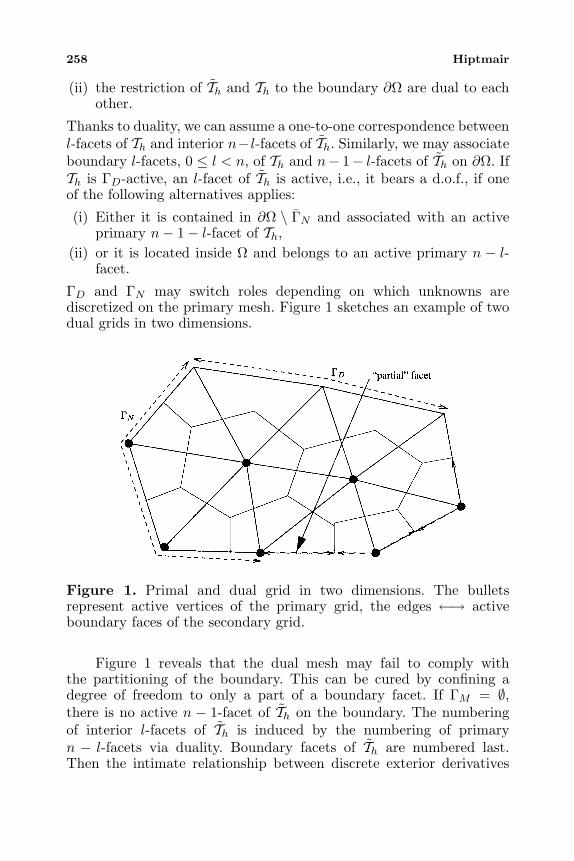
258 Hiptmair
(ii) the restriction of Th and Th to the boundary ∂Ω are dual to eachother.
Thanks to duality, we can assume a one-to-one correspondence betweenl-facets of Th and interior n− l-facets of Th. Similarly, we may associateboundary l-facets, 0 ≤ l < n, of Th and n− 1− l-facets of Th on ∂Ω. IfTh is ΓD-active, an l-facet of Th is active, i.e., it bears a d.o.f., if oneof the following alternatives applies:
(i) Either it is contained in ∂Ω \ ΓN and associated with an activeprimary n− 1− l-facet of Th,
(ii) or it is located inside Ω and belongs to an active primary n − l-facet.
ΓD and ΓN may switch roles depending on which unknowns arediscretized on the primary mesh. Figure 1 sketches an example of twodual grids in two dimensions.
Figure 1. Primal and dual grid in two dimensions. The bulletsrepresent active vertices of the primary grid, the edges ←→ activeboundary faces of the secondary grid.
Figure 1 reveals that the dual mesh may fail to comply withthe partitioning of the boundary. This can be cured by confining adegree of freedom to only a part of a boundary facet. If ΓM = ∅,there is no active n − 1-facet of Th on the boundary. The numberingof interior l-facets of Th is induced by the numbering of primaryn − l-facets via duality. Boundary facets of Th are numbered last.Then the intimate relationship between discrete exterior derivatives
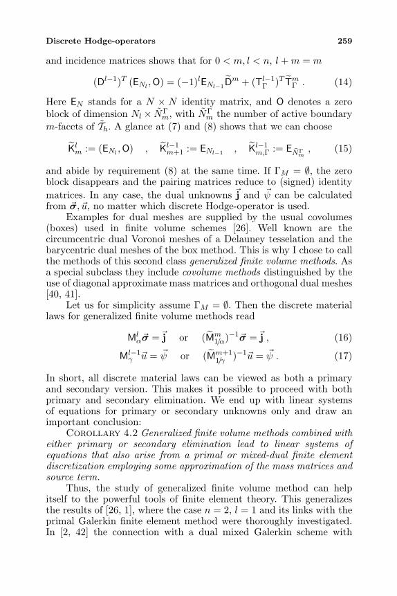
Discrete Hodge-operators 259
and incidence matrices shows that for 0 < m, l < n, l +m = m
(Dl−1)T (ENl ,O) = (−1)lENl−1Dm + (Tl−1
Γ )T TmΓ . (14)
Here EN stands for a N × N identity matrix, and O denotes a zeroblock of dimension Nl × NΓ
m, with NΓm the number of active boundary
m-facets of Th. A glance at (7) and (8) shows that we can choose
Klm := (ENl ,O) , Kl−1m+1 := ENl−1
, Kl−1m,Γ := ENΓ
m, (15)
and abide by requirement (8) at the same time. If ΓM = ∅, the zeroblock disappears and the pairing matrices reduce to (signed) identitymatrices. In any case, the dual unknowns j and ψ can be calculatedfrom σ, u, no matter which discrete Hodge-operator is used.
Examples for dual meshes are supplied by the usual covolumes(boxes) used in finite volume schemes [26]. Well known are thecircumcentric dual Voronoi meshes of a Delauney tesselation and thebarycentric dual meshes of the box method. This is why I chose to callthe methods of this second class generalized finite volume methods. Asa special subclass they include covolume methods distinguished by theuse of diagonal approximate mass matrices and orthogonal dual meshes[40, 41].
Let us for simplicity assume ΓM = ∅. Then the discrete materiallaws for generalized finite volume methods read
Mlασ =j or (Mm
1/α)−1σ =j , (16)
Ml−1γ u = ψ or (Mm+1
1/γ )−1u = ψ . (17)
In short, all discrete material laws can be viewed as both a primaryand secondary version. This makes it possible to proceed with bothprimary and secondary elimination. We end up with linear systemsof equations for primary or secondary unknowns only and draw animportant conclusion:
Corollary 4.2 Generalized finite volume methods combined witheither primary or secondary elimination lead to linear systems ofequations that also arise from a primal or mixed-dual finite elementdiscretization employing some approximation of the mass matrices andsource term.
Thus, the study of generalized finite volume method can helpitself to the powerful tools of finite element theory. This generalizesthe results of [26, 1], where the case n = 2, l = 1 and its links with theprimal Galerkin finite element method were thoroughly investigated.In [2, 42] the connection with a dual mixed Galerkin scheme with
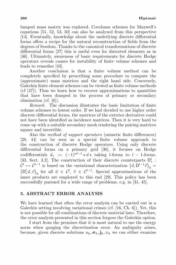
260 Hiptmair
lumped mass matrix was explored. Covolume schemes for Maxwell’sequations [51, 52, 53, 50] can also be analyzed from this perspective[14]. Eventually, knowledge about the underlying discrete differentialforms offers a recipe for the natural reconstruction of fields from thedegrees of freedom. Thanks to the canonical transformations of discretedifferential forms [27] this is useful even for distorted elements as in[46]. Ultimately, awareness of basic requirements for discrete Hodgeoperators reveals causes for instability of finite volume schemes andleads to remedies [43].
Another conclusion is that a finite volume method can becompletely specified by prescribing some procedure to compute the(approximate) mass matrices and the right hand side. Conversely,Galerkin finite element schemes can be viewed as finite volume methods(cf [47]). Thus we learn how to recover approximations to quantitiesthat have been dumped in the process of primary or secondaryelimination (cf. [6]).
Remark. The discussion illustrates the basic limitation of finitevolume schemes to lowest order. If we had decided to use higher orderdiscrete differential forms, the matrices of the exterior derivative couldnot have been identified as incidence matrices. Then it is very hard tocome up with a suitable secondary mesh rendering the pairing matricessquare and invertible.
Also the method of support operators (mimetic finite differences)[28, 44] can be seen as a special finite volume approach tothe construction of discrete Hodge operators. Using only discretedifferential forms on a primary grid [30], it focuses on Hodgecodifferentials d∗ := (−1)nl−1 d taking l-forms to l − 1-forms.[33, Sect. 3.2]. The construction of their discrete counterparts Dl
∗ :Cl → Cl−1 is based on the variational characterization
(u,Dl−1v
)0
=(Dl∗u,v
)0
for all u ∈ Cl, v ∈ Cl−1. Special approximations of theinner products are employed to this end [29]. This policy has beensuccessfully pursued for a wide range of problems, e.g. in [31, 45].
5. ABSTRACT ERROR ANALYSIS
We have learned that often the error analysis can be carried out in aGalerkin setting involving variational crimes (cf. [16, Ch. 6]). Yet, thisis not possible for all combinations of discrete material laws. Therefore,the error analysis presented in this section forgoes the Galerkin option.
I start from the premises that it is most natural to use the energynorm when gauging the discretization error. An ambiguity arises,because, given discrete solutions uh,σh, jh, ψh we can either examine
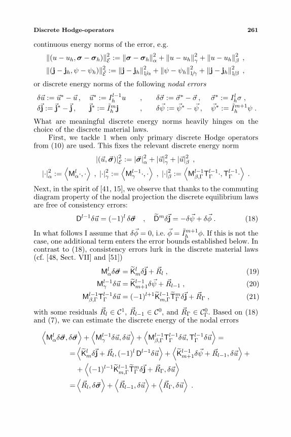
Discrete Hodge-operators 261
continuous energy norms of the error, e.g.
‖(u− uh,σ − σh)‖2E := ‖σ − σh‖2α + ‖u− uh‖2γ + ‖u− uh‖2β ,‖(j− jh, ψ − ψh)‖2E := ‖j− jh‖21/α + ‖ψ − ψh‖21/γ + ‖j− jh‖21/β ,
or discrete energy norms of the following nodal errors
δu := u∗ − u , u∗ := I l−1h u , δσ := σ∗ − σ , σ∗ := I lhσ ,
δj :=j∗ −j , j∗ := Imh j , δ ψ := ψ∗ − ψ , ψ∗ := Im+1h ψ .
What are meaningful discrete energy norms heavily hinges on thechoice of the discrete material laws.
First, we tackle 1 when only primary discrete Hodge operatorsfrom (10) are used. This fixes the relevant discrete energy norm
|(u, σ)|2E := |σ|2α + |u|2γ + |u|2β ,
|·|2α :=⟨Mlα·, ·
⟩, |·|2γ :=
⟨Ml−1γ ·, ·
⟩, |·|2β :=
⟨Ml−1β,ΓTl−1
Γ ·,Tl−1Γ ·
⟩.
Next, in the spirit of [41, 15], we observe that thanks to the commutingdiagram property of the nodal projection the discrete equilibrium lawsare free of consistency errors:
Dl−1δu = (−1)l δσ , Dmδj = −δ ψ + δφ . (18)
In what follows I assume that δφ = 0, i.e. φ = Im+1h φ. If this is not the
case, one additional term enters the error bounds established below. Incontrast to (18), consistency errors lurk in the discrete material laws(cf. [48, Sect. VII] and [51])
Mlαδσ = Klmδ
j + Rl , (19)
Ml−1γ δu = Kl−1
m+1δψ + Rl−1 , (20)
Ml−1β,ΓTl−1
Γ δu = (−1)l+1Kl−1m,ΓTmΓ δ
j + RΓ , (21)
with some residuals Rl ∈ C1, Rl−1 ∈ C0, and RΓ ∈ C0Γ. Based on (18)
and (7), we can estimate the discrete energy of the nodal errors⟨Mlαδσ, δσ
⟩+
⟨Ml−1γ δu, δu
⟩+
⟨Ml−1β,ΓTl−1
Γ δu,Tl−1Γ δu
⟩=
=⟨Klmδ
j + Rl, (−1)l Dl−1δu⟩
+⟨Kl−1m+1δ
ψ + Rl−1, δu⟩
+
+⟨(−1)l−1Kl−1
m,ΓTmΓ δj + RΓ, δu
⟩
=⟨Rl, δσ
⟩+
⟨Rl−1, δu
⟩+
⟨RΓ, δu
⟩.
262 Hiptmair
Please note that the second terms on both sides do not occur in the caseγ = 0 and an error estimate for u remains elusive. Hardly surprising,because there might not be a unique solution for u, unless specialproperties of Dl−1 (injectivity) are known. By the Cauchy-Schwarzinequality
|(δu, δσ)|E ≤∣∣∣(Ml
α)−1 Rl
∣∣∣α
+∣∣∣(Ml−1
γ )−1 Rl−1
∣∣∣γ
+∣∣∣(Ml−1
β,Γ)−1 RΓ
∣∣∣β.
Similar considerations apply, when solely secondary discreteHodge operators from (11) are employed. Then the suitable discreteenergy norm is given by∣∣∣(j, ψ)
∣∣∣2E
:=∣∣∣j
∣∣∣21/α
+∣∣∣ψ
∣∣∣21/γ
+∣∣∣j
∣∣∣21/β,
|·|21/α :=⟨Mm
1/α·, ·⟩, |·|21/γ :=
⟨Mm+1
1/γ ·, ·⟩, |·|21/β :=
⟨Mm
1/β,Γ·, ·⟩.
Partly retaining the notations for the consistency errors, we can write
Mm1/αδj =(−1)mn−m Kml δσ + Rm (22)
Mm+11/γ δ ψ =(−1)(l−1)(n−1) Km+1
l−1 δu+ Rm+1 (23)
Mm1/β,ΓTmΓ δ
j =(−1)(l−1)(n−1) Kml−1,ΓTl−1Γ δu+ RΓ , (24)
with Rm ∈ Cm, Rm+1 ∈ Cm+1, and RΓ ∈ CmΓ . Since (18) remains valid,the following identity is established as above:⟨
Ml1/αδj, δj
⟩+
⟨Ml−1
1/γ δψ, δ ψ
⟩+
⟨Ml−1
1/β,ΓTmΓ δj, TmΓ δj
⟩=
=⟨Rm, δj
⟩+
⟨Rm+1, δ ψ
⟩+
⟨RΓ, δj
⟩.
Other combinations of discrete material laws are treated alike. Forthe sake of brevity I am not elaborating on this. In sum, estimatingthe consistency errors of the material laws is the key to controllingdiscrete energy norms of nodal errors. The analysis of finite volumemethods [40, 41, 37] is often content with this goal, but I am not(cf. the discussion in [15, Sect. III]). Discrete energies might lack anyphysical meaning, so that the focus should be on the exact energynorm. In the case of primary discrete Hodge operators
‖(u− uh,σ − σh)‖E ≤ ‖(u− u∗h,σ − σ∗h)‖E + ‖(δuh, δσh)‖Etells us that it is essential to have stability
‖(uh,σh)‖E ≤ C |(u, σ)|E ∀u ∈ Cl−1, σ ∈ Cl , (25)
Discrete Hodge-operators 263
in order to get information about the energy of the total discretizationerror. Here, the constant C > 0 should be independent of as muchgeometric parameters of the mesh as possible. In the case of secondarydiscrete constitutive laws, we proceed as above, replacing ‖·‖E by ‖·‖Eand |·|E by |·|E .
In addition, the energy of the projection error ‖(u− u∗h,σ − σ∗h)‖Ehas to be bounded. This is the objective of asymptotic finite elementinterpolation estimates. Those rely on a Sobolev space setting andare large based on the Bramble-Hilbert lemma and affine equivalencetechniques depending on families of quasiuniform and shape regularmeshes [16, Ch. 4], [21, Ch. 3]. In particular, for results on discrete2-forms in two and three dimensions the reader should consult [17].Estimates for discrete 1-forms (n = 3) can be found in [38, 25, 22, 36].It is important to be aware that all estimates hinge on assumptions onthe smoothness of the continuous solutions.
In the case of finite difference or finite volume methods, one mightobject that the spaces of discrete differential forms are “artificial” andso is the notion of a total discretization error. Yet, an approximationof the total energy must always be available and the error in theapproximation of the total energy is well defined at any rate. For thiserror we get in the case of primary discrete Hodge operators
‖(u,σ)‖2E − |(u, σ)|2E =
= ‖(u,σ)‖2E − ‖(u∗h,σ∗h)‖2E + ‖(u∗h,σ∗h)‖2E −
− |(u∗, σ∗)|2E + |(u∗, σ∗)|2E − |(u, σ)|2E≤‖(u− u∗h,σ − σ∗h)‖E ‖(u+ u∗h,σ + σ∗h)‖E +
+ |(u∗ − u, σ∗ − σ)|E |(u∗ − u, σ∗ − σ)|E +
+ ‖(u∗h,σ∗h)‖2E − |(u∗, σ∗)|2E .
Even if the discretization error, the nodal error, and the projectionerror tend to zero, the error in the energy need not, owing to thequantity ‖(u∗h,σ∗h)‖
2E − |(u∗, σ
∗)|2E . It can be regarded as a consistencyerror in the approximation of the mass matrices. Hence, the quality ofthe approximation of the discrete energy can serve as an acid test forthe efficacy of a discretization scheme.
Remark. Primary Hodge operators do not permit us to get errorestimates for dual quantities. However, the generalized finite volumemethods are an exception. For instance, in the case ΓM = ∅ the boundfor |(δu, δσ)|E also applies to
⟨(Ml
α)−1δj, δj⟩
+⟨(Ml−1
γ )−1δ ψ, δ ψ⟩
+⟨(Ml−1
β,Γ)−1TmΓ δj, TmΓ δj
⟩.
264 Hiptmair
This paves the way for coming to terms with ‖(j− jh, ψ − ψh)‖2E .
6. ESTIMATION OF CONSISTENCY ERRORS
Let us study the consistency error term Rl from (19) and find boundsfor the relevant primary norm
∣∣∣(Mlα)−1 Rl
∣∣∣α. As a consequence of (18),
it is immediate that∣∣∣(Mlα)−1 Rl
∣∣∣2α
=⟨Mlα(σ∗ − ζ), σ∗ − ζ
⟩, (26)
where I set ζ := (Mlα)−1Klm
j∗. Note that by the definition of the weaksolution (cf. (2)) (σ,η)α =
∫Ω j∧ η for all η ∈ Hl(d,Ω). A few formal
manipulations yield
∣∣∣(Mlα)−1 Rl
∣∣∣α
= supη∈Cl
⟨Mlα(σ∗ − ζ), η
⟩|η|α
=
= supη∈Cl
1|η|α
(⟨Mlασ∗, η
⟩−
⟨Klmj∗, η
⟩)
= supη∈Cl
1|η|α
(⟨Mlασ∗, η
⟩− (σ∗,ηh)α + (σ∗ − σ,ηh)α +
+∫Ω
j ∧ ηh −∫Ω
j∗h ∧ ηh +∫Ω
j∗h ∧ ηh −⟨Klmj∗, η
⟩ )
≤ supη∈Cl
⟨Mlασ∗, η
⟩− (σ∗,ηh)α|η|α
+ supη∈Cl
∫Ω
j∗h ∧ ηh −⟨Klmj∗, η
⟩
|η|α+
+ supη∈Cl
‖ηh‖α|η|α
·(‖σ − σ∗h‖α + ‖j− j∗h‖1/α
)
The first two terms are typical consistency errors, as they occur inestimates for inexact finite element schemes [16, Ch. 8]. The factor infront of the third term reflects the stability of the approximate massmatrix Ml
α , whereas the third term itself incorporates approximationerrors of the nodal projection. In the case of an exact Galerkinapproach, the consistency terms and the stability factor can bedropped. Then, in combination with the results of the previous section,a standard finite element error estimate pops up.
Discrete Hodge-operators 265
There is a more direct approach to bounding the norm from(26), which is particularly useful in the case of diagonal finite volumemethods (cf. [40, 41]). So let us assume that Klm is an identity matrixand Ml
α is diagonal. For an l-facet F let F stand for its associated dualn − l-facet. Remember that the components of vectors in Cl can beindexed by the l-facets in Fl. By definition of Rl
∣∣∣(Mlα)−1 Rl
∣∣∣2α
=∑F∈Fl
mFR2l,F ,
Rl,F := m−1F σ
∗F −j∗F , (27)
with mF the diagonal element of Mlα belonging to F , and a subscript
F acting as a selector for vector components. Plugging in the canonicaldegrees of freedom for Whitney forms, we arrive at
Rl,F = m−1F
∫F
σ −∫
F
j = m−1F
∫F
σ −∫
F
α σ . (28)
In the spirit of finite difference methods, the final term may be tackledbased on a Taylor’s expansion of σ. If possible, it should be arounda suitable point in space, provided by the intersection of F andF . Sufficient smoothness of σ is tacitly assumed. An alternative toTaylor’s expansion are Bramble-Hilbert techniques, which impose lessstringent requirements on smoothness. However, shape-regularity ofthe meshes is indispensable then [40].
It is worth noting that (28) offers a prescription for a viable choiceof Ml
α. For instance, one could try to fix all mF such that Rl,F , F ∈ Fl,vanishes for any constant σ. However, the space of constant l-formshas dimension
(nl
). As 0 < l < n, this objective cannot be achieved in
general. Consider the case of a constant metric α and flat facets. If σis constant, too, (28) means
Rl,F = m−1F volα(F )σ(t1, . . . , tl)− volα(F )σ(n1, . . . ,nl) , (29)
where t1, . . . , tl and n1, . . . ,nl are α-orthonormal (oriented) basesof the tangent space of F and of the orthogonal complement of thetangent space of F . Only if Span t1, . . . , tl = Span n1, . . . ,nl,i.e. if F and F are α-orthogonal, we can make Rl,F vanish for allalternating l-linear forms σ. This highlights the necessity of orthogonaldual meshes, if diagonal approximate mass matrices are desired. (cf.[15, Sect. III]).
266 Hiptmair
REFERENCES
1. Bank, R. and D. Rose, “Some error estimates for the box method,”SIAM J. Numer. Anal., Vol. 24, 777–787, 1987.
2. Baranger, J., J.-F. Maitre, and F. Oudin, “Connection betweenfinite volume and mixed finite element methods,” RAIRO,Modelisation Math. Anal. Numer., Vol. 30, 445–465, 1996.
3. Bossavit, A., “Mixed finite elements and the complex of Whitneyforms,” The Mathematics of Finite Elements and Applications VI,J. Whiteman (ed.), 137–144, Academic Press, London, 1988.
4. Bossavit, A., “A new viewpoint on mixed elements,” Meccanica,Vol. 27, 3–11, 1992.
5. Bossavit, A., Computational Electromagnetism. Variational For-mulation, Complementarity, Edge Elements, No. 2 in AcademicPress Electromagnetism Series, Academic Press, San Diego, 1998.
6. Bossavit, A., “How weak is the weak solution in finite elementmethods?” IEEE Trans. Magnetics, Vol. MAG-34, 2429–2432,1998.
7. Bossavit, A., “On the geometry of electromagnetism IV:‘Maxwell’s house’,” J. Japan Soc. Appl. Electromagnetics &Mech., Vol. 6, 318–326, 1998.
8. Bossavit, A., “On the geometry of electromagnetism I: Affinespace,” J. Japan Soc. Appl. Electromagnetics & Mech., Vol. 6,17–28, 1998.
9. Bossavit, A., “On the geometry of electromagnetism II:Geometrical objects,” J. Japan Soc. Appl. Electromagnetics &Mech., Vol. 6, 114–123, 1998.
10. Bossavit, A., “On the geometry of electromagnetism III:Integration, Stokes’, Faraday’s law,” J. Japan Soc. Appl.Electromagnetics & Mech., Vol. 6, 233–240, 1998.
11. Bossavit, A., “Computational electromagnetism and geometry.Building a finite-dimensional “Maxwell’s house” I: Networkequations,” J. Japan Soc. Appl. Electromagnetics & Mech., Vol.7, 150–159, 1999.
12. Bossavit, A., “Computational electromagnetism and geometry II:Network constitutive laws,” J. Japan Soc. Appl. Electromagnetics& Mech., Vol. 7, 294–301, 1999.
13. Bossavit, A., “Generalized finite differences in computationalelectromagnetics,” this volume.
14. Bossavit, A. and L. Kettunen, “Yee–like schemes on a tetrahedralmesh with diagonal lumping,” Int. J. Numer. Modelling, Vol. 12,
Discrete Hodge-operators 267
129–142, 1999.15. Bossavit, A. and L. Kettunen, “Yee-like schemes on staggered
cellular grids: A synthesis between FIT and FEM approaches,”contribution to COMPUMAG ’99., 1999.
16. Brenner, S. and R. Scott, Mathematical Theory of Finite ElementMethods, Texts in Applied Mathematics, Springer-Verlag, NewYork, 1994.
17. Brezzi, F. and M. Fortin, Mixed and Hybrid Finite ElementMethods, Springer-Verlag, 1991.
18. Burke, W., Applied Differential Geometry, Cambridge UniversityPress, Cambridge, 1985.
19. Cartan, H., Formes Differentielles, Hermann, Paris, 1967.20. Chew, W., “Electromagnetic theory on a lattice,” J. Appl. Phys.,
Vol. 75, 4843–4850, 1994.21. Ciarlet, P., “The finite element method for elliptic problems,”
Studies in Mathematics and its Applications, Vol. 4, North-Holland, Amsterdam, 1978.
22. Ciarlet, Jr., P. and J. Zou, “Fully discrete finite elementapproaches for time-dependent Maxwell equations,” Numer.Math., Vol. 82, 193–219, 1999.
23. De La Bourdonnay, A. and S. Lala, “Duality between finiteelements and finite volumes and Hodge operator,” NumericalMethods in Engineering ’96, 557–561, Wiley & Sons, Paris, 1996.
24. Dezin, A., Multidimensional Analysis and Discrete Models, CRCPress, Boca Raton, FL, USA, 1995.
25. Girault, V. and P. Raviart, Finite Element Methods for Navier-Stokes Equations, Springer-Verlag, Berlin, 1986.
26. Hackbusch, W., “On first and second order box schemes,”Computing, Vol. 41, 277–296, 1989.
27. Hiptmair, R., “Canonical construction of finite elements,” Math.Comp., Vol. 68, 1325–1346, 1999.
28. Hyman, J. and S. Steinberg, “The numerical solution of diffusionproblems in strongly heterogeneous non-isotropic materials,” J.Comp. Phys., Vol. 132, 130–148, 1997.
29. Hyman, J. and M. Shashkov, “Adjoint operators for the naturaldiscretizations of the divergence, gradient and curl on logicallyrectangular grids,” Applied Numerical Mathematics, Vol. 25, 413–442, 1997.
30. Hyman, J. and M. Shashkov, “Natural discretizations forthe divergence, gradient, and curl on logically rectangulargrids,” International Journal of Computers & Mathematics with
268 Hiptmair
Applications, Vol. 33, 81–104, 1997.31. Hyman, J. and M. Shashkov, “Mimetic discretizations for
Maxwell’s equations,” J. Comp. Phys., Vol. 151, 881–909, 1999.32. Hyman, J. and M. Shashkov, “The orthogonal decomposition
theorems for mimetic finite difference methods,” SIAM Journalon Numerical Analysis, Vol. 36, 788–818, 1999.
33. Iwaniec, T., “Nonlinear differential forms,” Lectures notes of theInternational Summer School in Jyvaskyla, 1998 80, Departmentof Mathematics, University of Jyvaskyla, Jyvaskyla, Finland,1999.
34. Lala, S. and A. de la Bourdonnaye, “A finite-element methodfor Maxwell system preserving Gauss laws and energy,” Tech.Rep. RR-3557, INRIA, Sophia Antipolis, France, November 1998.Submitted to Numer. Math.
35. Mattiussi, C., “An analysis of finite volume, finite element, andfinite difference methods using some concepts from algebraictopology,” J. Comp. Phys., Vol. 9, 295–319, 1997.
36. Monk, P., “An analysis of Nedelec’s method for the spatialdiscretization of Maxwell’s equations,” J. Comp. Appl. Math.,Vol. 47, 101–121, 1993.
37. Monk, P. and E. Suli, “A convergence analysis of Yee’s schemeon nonuniform grids,” SIAM J. Numer. Anal., Vol. 31, 393–412,1994.
38. Nedelec, J., “Mixed finite elements in R3,” Numer. Math., Vol. 35,315–341, 1980.
39. Nicolaides, R., “Direct discretization of planar div-curl problems,”SIAM J. Numer. Anal., Vol. 29, 32–56, 1992.
40. Nicolaides, R. and D.-Q. Wang, “Convergence analysis of acovolume scheme for Maxwell’s equations in three dimensions,”Math. Comp., Vol. 67, 947–963, 1998.
41. Nicolaides, R. and X. Wu, “Covolume solutions of three-dimensional div-curl equations,” SIAM J. Numer. Anal., Vol. 34,2195–2203, 1997.
42. Sacco, R. and F. Saleri, “Exponentially fitted shape functionsfor advection-dominated flow problems in two dimensions,” J.Comput. Appl. Math., Vol. 67, 161–165, 1996.
43. Schuhmann, R. and T. Weiland, “A stable interpolation techniquefor FDTD on non-orthogonal grids,” Int. J. Numer. Model.,Vol. 11, 299–306, 1998.
44. Shashkov, M., Conservative Finite-Difference Methods on GeneralGrids, CRC Press, Boca Raton, 1996.
Discrete Hodge-operators 269
45. Shashkov, M. and S. Steinberg, “Solving diffusion equations withrough coefficients in rough grids,” J. Comp. Phys., Vol. 129, 383–405, 1996.
46. Shashkov, M., B. Swartz, and B. Wendroff, “Local reconstructionof a vector field from its components on the faces of grid cells,”Journal of Computational Physics, Vol. 139, 406–408, 1998.
47. Tarhasaari, T., L. Kettunen, and A. Bossavit, “Some realizationsof a discrete Hodge: A reinterpretation of finite elementtechniques,” IEEE Trans. Mag., Vol. 35, 1494–1497, 1999.
48. Teixeira, F. and W. Chew, “Lattice electromagnetic theory froma topological viewpoint,” J. Math. Phys., Vol. 40, 169–187, 1999.
49. Tonti, E., “On the geometrical structure of electromagnetism,”Graviation, Electromagnetism and Geometrical Structures, G. Fer-rarese (ed.), 281–308, Pitagora, Bologna, Italy, 1996.
50. van Rienen, U., “Finite integration technique on triangular gridsrevisited,” Int. J. Numer. Model., Vol. 12, 107–128, 1999.
51. Weiland, T., “Die Diskretisierung der Maxwell-Gleichungen,”Phys. Bl., Vol. 42, 191–201, 1986.
52. Weiland, T., “Time domain electromagnetic field computationwith finite difference methods,” Int. J. Numer. Modelling, Vol.9, 295–319, 1996.
53. Yee, K., “Numerical solution of initial boundary value problemsinvolving Maxwell’s equations in isotropic media,” IEEE Trans.Antennas and Propagation, Vol. 16, 302–307, 1966.
Progress In Electromagnetics Research, PIER 32, 271–299, 2001
HIGHER ORDER WHITNEY FORMS
R. Hiptmair
Sonderforschungsbereich 382Universitat Tubingen72076 Tuebingen, Germany
Abstract—The calculus of differential forms can be used to devisea unified description of discrete differential forms of any order andpolynomial degree on simplicial meshes in any spatial dimension.A general formula for suitable degrees of freedom is also available.Fundamental properties of nodal interpolation can be establishedeasily. It turns out that higher order spaces, including variants withlocally varying polynomial order, emerge from the usual Whitney-forms by local augmentation. This paves the way for an adaptive p-version approach to discrete differential forms.
1 Introduction
2 Exterior Calculus
3 Local Spaces
4 Degrees of Freedom
5 Hierarchical Bases
References
1. INTRODUCTION
It is generally acknowledged that the calculus of differential forms isthe right device for mathematical modeling in many fields of physics,in particular in electromagnetism [8, 3, 14]. For instance, it turns outthat the electric field should be regarded as a 1-form, and that thedifferential operators div and curl are just different manifestations ofthe exterior derivative d of differential forms.
As differential forms capture the nature of continuous fields, it isnatural to resort to discrete differential forms when approximations
272 Hiptmair
of these fields are desired. Here, “discrete” means that the form iscompletely determined by only a finite number of degrees of freedom.By definition, the basic relationships of the calculus of differential formsmust hold for the discrete differential forms. Thus, essential propertiesof the continuous physical models like conservation principles arepreserved in the discrete setting.
Special discrete differential forms that are associated withtriangulations of a computational domain give rise to finite elementsthat offer appropriate spaces for the corresponding physical quantities.For instance, they supply the hugely popular edge elements ofcomputational electromagnetism. In conjunction with variationalprinciples, discrete differential forms thus become a powerful tool forthe approximate numerical solution of boundary value problems.
With hindsight, it is startling that after the discovery of discretedifferential forms by Whitney [27] it took a long time before theirsignificance as computational tool was realized [6, 7]. Without referringto differential geometry, several authors [22, 23, 25] had devised vectorvalued finite elements that can be regarded as special cases of discretedifferential forms. Their constructions are formidably intricate andrequire much technical effort.
A substantial simplification can be achieved as was demonstratedin [18]: One should exploit the facilities provided by differentialgeometry for a completely coordinate-free treatment of discretedifferential forms. Once we have shed the cumbersome vector calculus,everything can be constructed and studied with unmatched generalityand elegance. In particular, all orders of forms and all degrees ofpolynomial approximation can be dealt with in the same framework.This can be done for simplicial meshes in arbitrary dimension.
The purpose of this paper is twofold. First the results in [18] shouldbe made accessible to a wider audience beyond theoretical numericalanalysts. Secondly, special attention is paid to discrete differentialforms of higher polynomial degree. The rationale is the arrival of so-called p-adaptive finite element schemes. Their principle is to adjust thepolynomial degree of the approximating finite elements to local featuresof the solution in order to gain accuracy with minimum costs. Whenthis idea is to be applied to discrete differential forms it becomes vitalto know suitable local basis functions for various polynomial degrees.Higher order discrete differential forms also form the foundation ofhierarchical a-posteriori error estimators [4].
This paper complements and caps several earlier investigationsinto the subject of higher order edge elements [1, 13, 17, 24, 16, 20,28, 26]. However, it does not discuss special schemes, but emphasizesgoverning principles. Once these are understood, they offer guidance
Higher order Whitney forms 273
on how to tailor higher order discrete differential forms to particularneeds.
I should stress that the entire presentation is set in a purely affinecontext and, consequently, never resorts to vectorfields or functionsrepresenting differential forms. This is in stark contrast with the usualtreatment of higher order discrete differential forms in literature. Thusmy exposure might strike many a reader as peculiar. Yet, metricstructures are alien to discrete differential forms. Of course, ultimatelyorthogonal coordinates come handily for actual computations, butintroducing them already for the construction of discrete differentialforms distracts from generic properties.
2. EXTERIOR CALCULUS
This section summarizes a few fundamental concepts of exteriorcalculus. It does not attempt to give an introduction to the subject.For a comprehensive discussion of the theory of differential forms seethe monograph [11] or consult your favorite textbook on advanceddifferential calculus.
In the most general sense, Ω may be a (piecewise) smooth orientedand bounded n-dimensional Riemannian manifold, n ∈ N, with apiecewise smooth boundary. A differential form ω of order l, 0 ≤ l ≤ n,is a mapping from Ω into the
(nl
)-dimensional space l(TΩ(x)) of
alternating l–multilinear forms on the n-dimensional tangent spaceTΩ(x) at Ω in x ∈ Ω [11, Sect. 2.1]. In the sequel, Dl
k(Ω) stands for thespace of l-forms on Ω of class Ck.
A fundamental concept in the theory of differential forms is theintegral of a p-form over a piecewise smooth p-dimensional orientedmanifold. Through integration a differential form assigns a value toeach suitable manifold, modeling the physical procedure of measuringa field. We write Dl(Ω) for the vector space of l-forms on Ω,whose Riemann-integrals exist for any compact piecewise smooth l-dimensional submanifold of Ω.
From alternating l-multilinear forms differential l-forms inherit theexterior product ∧ : Dl
0(Ω) × Dk0(Ω) → Dl+k
0 (Ω), 0 ≤ l, k, l + k ≤ n,defined in a pointwise sense. Moreover, remember that the trace tΣωof an l-form ω ∈ Dl(Ω), 0 ≤ l < n, onto some piecewise smooth n− 1-dimensional submanifold Σ ⊂ Ω yields an l-form on Σ [19, Sect. 1.10].It can be introduced by restricting ω(x) ∈ l(TΩ(x)), x ∈ Σ, to thetangent space of Σ in x. The trace commutes with the exterior productand exterior differentiation, i.e. d tΣω = tΣdω for ω ∈ Dl
1(Ω).Another crucial device is the exterior derivative d , a linear
mapping from differentiable l-forms into l + 1-forms. Moreover,
274 Hiptmair
Stokes’ theorem makes it possible to define the exterior derivativedω ∈ Dl+1(Ω) of ω ∈ Dl(Ω). A fundamental fact about exteriordifferentiation is that d(d ω) = 0 for any sufficiently smooth differentialform ω. Under some restrictions on the topology of Ω the converse isalso true:
Theorem 2.1(Poincare’s lemma) For a contractible domain Ω ⊂Rn every ω ∈ Dl
1(Ω), l ≥ 1, with dω = 0 is the exterior derivative ofan l − 1–form over Ω.
This result is sometimes referred to as the exact sequence property.A second main result about the exterior derivative is the integrationby parts formula [19, Sect. 3.2]
∫Ω
dω ∧ η + (−1)l∫Ω
ω ∧ dη =∫∂Ω
ω ∧ η (1)
for ω ∈ Dl(Ω), η ∈ Dk(Ω), 0 ≤ l, k < n − 1, l + k = n − 1. Here, theboundary ∂Ω is endowed with the induced orientation.
Finally, we recall the pullback ω → Φ∗ω under a changeof variables described by a diffeomorphism Φ. This transformationcommutes with both the exterior product and the exterior derivative,and it leaves the integral invariant.
3. LOCAL SPACES
Following the classical approach in the theory of finite elements [12],we first try to establish suitable spaces X l
k(T ) of discrete l-forms,0 ≤ l ≤ n, on individual simplices Ti of a triangulation Th := Tiof Ω ⊂ Rn. Here, k ∈ N0 stands for the “polynomial degree” of theforms, a notion that will be explained in a moment.
The transformation of differential forms immediately suggests thatwe should opt for a construction based on affine equivalence. Thismeans that the local spaces X l
k(T ) of discrete differential forms arefirst specified on some reference simplex T . An arbitrary simplex T
of the mesh Th can be mapped onto T by an affine transformationΦT : T → T . Then the corresponding pullback converts the discreteforms on T into those on T according to
X lk(T ) := Φ∗TX
lk(T ) . (2)
A tenet of affine equivalence is that the choice of T must not matter inthe end. The reader can always imagine T to be the simplex spanned by
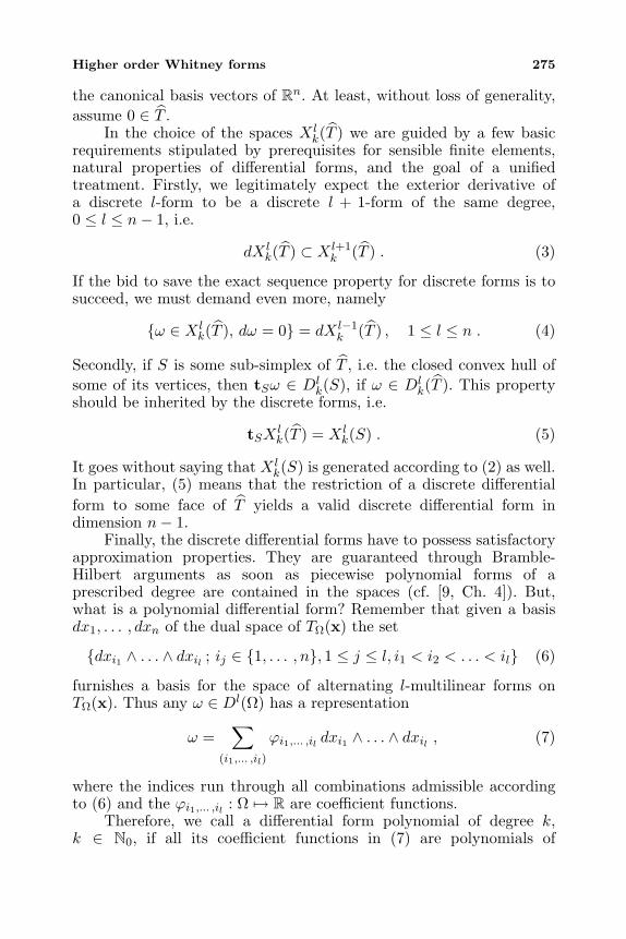
Higher order Whitney forms 275
the canonical basis vectors of Rn. At least, without loss of generality,assume 0 ∈ T .
In the choice of the spaces X lk(T ) we are guided by a few basic
requirements stipulated by prerequisites for sensible finite elements,natural properties of differential forms, and the goal of a unifiedtreatment. Firstly, we legitimately expect the exterior derivative ofa discrete l-form to be a discrete l + 1-form of the same degree,0 ≤ l ≤ n− 1, i.e.
dX lk(T ) ⊂ X l+1
k (T ) . (3)
If the bid to save the exact sequence property for discrete forms is tosucceed, we must demand even more, namely
ω ∈ X lk(T ), dω = 0 = dX l−1
k (T ) , 1 ≤ l ≤ n . (4)
Secondly, if S is some sub-simplex of T , i.e. the closed convex hull ofsome of its vertices, then tSω ∈ Dl
k(S), if ω ∈ Dlk(T ). This property
should be inherited by the discrete forms, i.e.
tSX lk(T ) = X l
k(S) . (5)
It goes without saying that X lk(S) is generated according to (2) as well.
In particular, (5) means that the restriction of a discrete differentialform to some face of T yields a valid discrete differential form indimension n− 1.
Finally, the discrete differential forms have to possess satisfactoryapproximation properties. They are guaranteed through Bramble-Hilbert arguments as soon as piecewise polynomial forms of aprescribed degree are contained in the spaces (cf. [9, Ch. 4]). But,what is a polynomial differential form? Remember that given a basisdx1, . . . , dxn of the dual space of TΩ(x) the set
dxi1 ∧ . . . ∧ dxil ; ij ∈ 1, . . . , n, 1 ≤ j ≤ l, i1 < i2 < . . . < il (6)
furnishes a basis for the space of alternating l-multilinear forms onTΩ(x). Thus any ω ∈ Dl(Ω) has a representation
ω =∑
(i1,... ,il)
ϕi1,... ,il dxi1 ∧ . . . ∧ dxil , (7)
where the indices run through all combinations admissible accordingto (6) and the ϕi1,... ,il : Ω → R are coefficient functions.
Therefore, we call a differential form polynomial of degree k,k ∈ N0, if all its coefficient functions in (7) are polynomials of
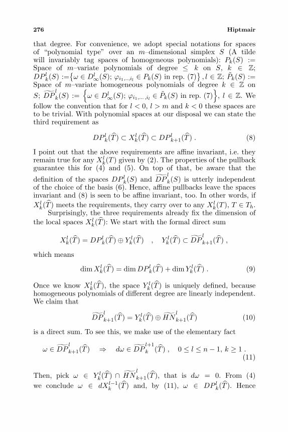
276 Hiptmair
that degree. For convenience, we adopt special notations for spacesof “polynomial type” over an m–dimensional simplex S (A tildewill invariably tag spaces of homogeneous polynomials): Pk(S) :=Space of m–variate polynomials of degree ≤ k on S, k ∈ Z;DP lk(S) :=
ω ∈ Dl
∞(S); ϕi1,..,il ∈ Pk(S) in rep. (7), l ∈ Z; Pk(S) :=
Space of m–variate homogeneous polynomials of degree k ∈ Z onS; DP
l
k(S) :=ω ∈ Dl
∞(S); ϕi1,... ,il ∈ Pk(S) in rep. (7)
, l ∈ Z. Wefollow the convention that for l < 0, l > m and k < 0 these spaces areto be trivial. With polynomial spaces at our disposal we can state thethird requirement as
DP lk(T ) ⊂ X lk(T ) ⊂ DP lk+1(T ) . (8)
I point out that the above requirements are affine invariant, i.e. theyremain true for any X l
k(T ) given by (2). The properties of the pullbackguarantee this for (4) and (5). On top of that, be aware that the
definition of the spaces DP lk(S) and DPl
k(S) is utterly independentof the choice of the basis (6). Hence, affine pullbacks leave the spacesinvariant and (8) is seen to be affine invariant, too. In other words, ifX lk(T ) meets the requirements, they carry over to any X l
k(T ), T ∈ Th.Surprisingly, the three requirements already fix the dimension of
the local spaces X lk(T ): We start with the formal direct sum
X lk(T ) = DP lk(T )⊕ Y l
k(T ) , Y lk(T ) ⊂ DP
l
k+1(T ) ,
which means
dimX lk(T ) = dimDP lk(T ) + dimY l
k(T ) . (9)
Once we know X lk(T ), the space Y l
k(T ) is uniquely defined, becausehomogeneous polynomials of different degree are linearly independent.We claim that
DPl
k+1(T ) = Y lk(T )⊕ HN l
k+1(T ) (10)
is a direct sum. To see this, we make use of the elementary fact
ω ∈ DP lk+1(T ) ⇒ dω ∈ DP l+1
k (T ) , 0 ≤ l ≤ n− 1, k ≥ 1 .(11)
Then, pick ω ∈ Y lk(T ) ∩ HN
l
k+1(T ), that is dω = 0. From (4)we conclude ω ∈ dX l−1
k (T ) and, by (11), ω ∈ DP lk(T ). Hence
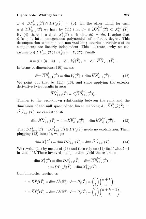
Higher order Whitney forms 277
ω ∈ DPl
k+1(T ) ∩ DP lk(T ) = 0. On the other hand, for each
η ∈ DPl
k+1(T ) we have by (11) that dη ∈ DPl+1
k (T ) ⊂ X l+1k (T ).
By (4) there is a φ ∈ X lk(T ) such that dφ = dη. Imagine that
φ is split into homogeneous polynomials of different degree. Thisdecomposition is unique and non-vanishing exterior derivatives of itscomponents are linearly independent. This illustrates, why we canassume φ ∈ DP lk+1(T ) ∩X l
k(T ) = Y lk(T ). Finally
η = φ+ (η − φ) , φ ∈ Y lk(T ) , η − φ ∈ HN l
k+1(T ) .
In terms of dimensions, (10) means
dim DPl
k+1(T ) = dimY lk(T ) + dim HN
l
k+1(T ) . (12)
We point out that by (11), (16), and since applying the exteriorderivative twice results in zero
HNl
k+1(T ) = d(DPl−1
k+2(T )) .
Thanks to the well–known relationship between the rank and thedimension of the null space of the linear mapping d : DP
l−1
k+2(T ) →HN
l
k+1(T ), we can establish
dim HNl
k+1(T ) = dim DPl−1
k+2(T )− dim HNl−1
k+2(T ) . (13)
That DP lk+1(T ) = DPl
k+1(T )⊕DP lk(T ) needs no explanation. Then,plugging (12) into (9), we get
dimX lk(T ) = dimDP lk+1(T )− dim HN
l
k+1(T ) . (14)
We rewrite (14) by means of (13) and then rely on (14) itself with l−1instead of l. These involved manipulations yield the recursion
dimX lk(T ) = dimDP lk+1(T )− dim DP
l−1
k+2(T ) +
dimDP l−1k+2(T )− dimX l−1
k+1(T ) .
Combinatorics teaches us
dimDP kl (T ) = diml(Rn) · dimPk(T ) =(n
l
)(n+ k
k
),
dim DPk
l (T ) = diml(Rn) · dim Pk(T ) =(n
l
)(n+ k − 1
k
).
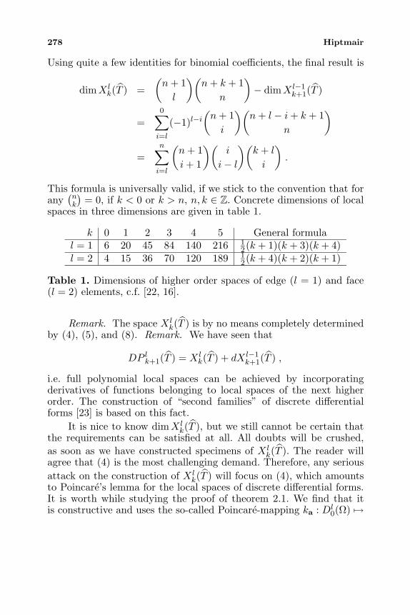
278 Hiptmair
Using quite a few identities for binomial coefficients, the final result is
dimX lk(T ) =
(n+ 1l
)(n+ k + 1
n
)− dimX l−1
k+1(T )
=0∑i=l
(−1)l−i(n+ 1i
)(n+ l − i+ k + 1
n
)
=n∑i=l
(n+ 1i+ 1
)(i
i− l
)(k + l
i
).
This formula is universally valid, if we stick to the convention that forany
(nk
)= 0, if k < 0 or k > n, n, k ∈ Z. Concrete dimensions of local
spaces in three dimensions are given in table 1.
k 0 1 2 3 4 5 General formulal = 1 6 20 45 84 140 216 1
2(k + 1)(k + 3)(k + 4)l = 2 4 15 36 70 120 189 1
2(k + 4)(k + 2)(k + 1)
Table 1. Dimensions of higher order spaces of edge (l = 1) and face(l = 2) elements, c.f. [22, 16].
Remark. The space X lk(T ) is by no means completely determined
by (4), (5), and (8). Remark. We have seen that
DP lk+1(T ) = X lk(T ) + dX l−1
k+1(T ) ,
i.e. full polynomial local spaces can be achieved by incorporatingderivatives of functions belonging to local spaces of the next higherorder. The construction of “second families” of discrete differentialforms [23] is based on this fact.
It is nice to know dimX lk(T ), but we still cannot be certain that
the requirements can be satisfied at all. All doubts will be crushed,as soon as we have constructed specimens of X l
k(T ). The reader willagree that (4) is the most challenging demand. Therefore, any seriousattack on the construction of X l
k(T ) will focus on (4), which amountsto Poincare’s lemma for the local spaces of discrete differential forms.It is worth while studying the proof of theorem 2.1. We find that itis constructive and uses the so-called Poincare-mapping ka : Dl
0(Ω) →
Higher order Whitney forms 279
Dl−11 (Ω), 0 < l ≤ n, for x ∈ Ω and vi ∈ Rn defined by
ka(ω)(x)(v1, ..,vl−1) :=
1∫0
tl−1ω(a + t(x− a))(x− a,v1, ..,vl−1) dt ,
(15)
to get a potential for the closed form ω. For ω ∈ Dl1(Ω), ka(ω) is a
valid l − 1–form and satisfies (cf. [11], Formula 2.13.2)
d(ka(ω)) + ka(dω) = ω . (16)
Sloppily speaking, the Poincare mapping is a sort of partial rightinverse of the exterior derivative, as d ka d = d.
It is immediately clear that the Poincare-mapping takespolynomial forms to other polynomial forms. Straightforward, buttedious computations reveal the details (cf. lemma 5 in [18]):
Lemma 3.1 For ω ∈ DPl
k(T ), k > 0, we know that ka(ω) ∈DP l−1
k+1(T ). In the special case a = 0, the even stronger assertion
k0(ω) ∈ DP l−1
k+1(T ) holds true.This motivates a tentative definition of Xk
l (T ) by
Xkl (T ) := DP lk(T ) + ka(DP l+1
k (T )) , a ∈ T .
Strictly speaking, this is not a valid definition before we have notshown that the choice of a ∈ T does not matter. First recall thatfor p ∈ Pk(T ) the difference p(·)− p(· − c) belongs to Pk−1(T ) for anyc ∈ Rn. Therefore we can decompose ω ∈ DP lk(T ) into
ω(a + t(x− a)) = ω(tx) + π(tx) ,
where π ∈ DP lk−1(T ). Using the definition of the potential mappingand the token • for l − 1 vectors from R
n, we get
ka(ω)(x)(•) = −1∫
0
tl−1 ω(a + t(x− a))(a, •)︸ ︷︷ ︸∈DP l−1
k (T )
dt
+
1∫0
tl−1 (ω(tx) + π(tx)) (x, •) dt
= k0(ω)(x)(•) + η(x)(•) ,
280 Hiptmair
with an η ∈ DP l−1k (T ) according to Lemma (3.1). In short, ka(ω) −
k0(ω) ∈ DP l−1k (T ) and the above definition makes sense. Alas, it fails
to meet the requirements: Let us introduce the space of homogeneouspolynomial differential forms belonging to the nullspace of the exteriorderivative
HNl
k(S) := ω ∈ DP lk(S); dω = 0 .
For 0 < l ≤ n − 2, k ≥ 1, pick η ∈ HNl+2
k−1(T ), set µ := k0(η)and conclude from (16) that µ = k0(dµ). In addition, lemma (3.1)
tells us that µ ∈ DPl+1
k (T ). Next, set ω := k0(µ), which means
dω = dk0(µ) = µ − k0(dµ) = 0 and ω ∈ DP lk+1(T ). Moreover, η = 0involves ω = 0, as the Poincare-mapping is injective. On the otherhand, we want to have ω ∈ d(DP l−1
k+1(T )) ⊂ DP lk(T ), which fails for
η = 0 as DP lk(T )∩ DP lk+1(T ) = 0. At least one of the requirements
is violated, if HNl+2
k−1(T ) = 0, which can be verified by elementary
calculations, since HNl+2
k−1(T ) = dDPl+1
k (T ).The tentative definition supplies a space that is simply too large.
Carefully inspecting its flaws, one finds that only closed forms shouldbe admitted as arguments to the Poincare-mapping. This leads us tothe improved definition
X lk(T ) := DP lk(T ) + ka
(HN
l+1
k (T ))
(17)
The point a ∈ T is arbitrary, but it does not make a difference, anyway.By lemma (3.1) it is obvious that (8) holds. Then, (3) is an immediateconsequence. To verify (4) keep in mind that we could have given theequivalent definition
X lk(T ) := DP lk(T ) + ka
(ω ∈ DP l+1
k (T ), dω = 0).
We also observe that thanks to lemma (3.1) the splitting
X lk(T ) := DP lk(T )⊕ k0
(HN
l+1
k (T ))
(18)
is direct, as homogeneous polynomials of different degree are linearlyindependent. Let ω ∈ X l
k(T ) with dω = 0 be split according to (18)
into ω = ω0 + ω. Since ω ∈ DPl
k+1(T ) and ω0 ∈ DP lk(T ), the
Higher order Whitney forms 281
linear independence of homogeneous polynomials of different degreecombined with lemma (3.1) shows that dω = 0. But ω = k0(η) for
η ∈ HN l+1
k (T ) and so (16) can be employed to get
η = dk0(η) + k0(dη) = dω + k0(0) = 0 ⇒ ω = 0 .
Eventually we have found ω = ω0 ∈ DP lk(T ) and arrive at
ω = dk0(ω) ∈ d(X l−1k (T )
).
To confirm the trace property (5) we consider one n − 1-dimensionalsubsimplex F , a face of T . Induction with respect to n will settleeverything else. Pick a in (17) as a vertex of F and note that x − abelongs to the tangent hyperplane of F . Thus, by the very definitionof the trace of a differential form
tF (ka(ω)) = ka(tFω) ∀ω ∈ Dl0(T ) .
Since obviously tF (DP lk(T )) = DP lk(F ), the identity X lk(F ) =
tFX lk(T ) follows.We now scrutinize a few special cases of local ansatz spaces
generated by formula (17): For l = n we get X lk(T ) = DP lk(T ),
since HNl+1
k (T ) = 0. Also in the case l = 0 we end up withcomplete polynomial spaces: For any ω ∈ D0
1(T ) with ω(0) = 0 wehave ω = k0(dω) by (16). Obviously this involves
k0(HN1
k(T )) = DP0
k+1(T ) ,
as dω ∈ HN1
k(T ) for all ω ∈ DP 0
k+1(T ). An easy consequence is thatin the case l = 0
X0k(T ) = DP 0
k(T ) + DP0
k+1(T ) = DP 0k+1(T ) ,
i.e. the full space of polynomials of degree ≤ k + 1.Example. An explicit construction of the local space X1
1 (T ) intwo dimensions can be carried out as follows: Using affine coordinatesx1, x2 we can write
DP2
1(T ) = ω(x) = (α1x1 + α2x2)dx1 ∧ dx2, α1, α2 ∈ R .
Note that in this case HN2
1(T ) = DP2
1(T ). If this did not hold,the condition dω = 0 would introduce some linear constraints for
282 Hiptmair
the coefficients α1 and α2. For ω = (α1x1 + α2x2)dx1 ∧ dx2 simplecomputations yield
k0(ω)(x) =
1∫0
t(α1tx1 + α2tx2)(dx1 ∧ dx2)(x, ·) dt
=13(α1x1 + α2x2)(x1dx2 − x2dx1) .
(19)
This means according to (17)
X11 (T ) =
ω =(γ1 + β11x1 + β12x2 − α1x1x2 − α2x22)dx1 +
+ (γ2 + β21x1 + β22x2 + α1x21 − α2x1x2)dx2,
γi, αi, βij ∈ R
.
Remark. Simple counterexamples show that in general
X lk(T ) = X0
0 (T ) ∧ . . . ∧X00 (T )︸ ︷︷ ︸
k−1 times
∧X l0(T ) .
As a technical tool we are going to need the local spaces of discretedifferential forms with vanishing trace on ∂T
H lk(T ) := ω ∈ X l
k(T ), t∂Tω = 0 .
It can be confirmed (cf. [18, Lemma 17]) that the local exact sequenceproperty applies to these spaces, as well
ω ∈ H lk(T ), dω = 0 = d H l−1
k (T ) , 0 ≤ l < n , (20)
ω ∈ Xnk (T ),
∫
T
ω = 0 = d Hn−1k (T ) . (21)
4. DEGREES OF FREEDOM
The previous section provided us with with local spaces X lk(T ) of l-
forms on the simplices T of a triangulation Th of Ω. The correspondingglobal space of finite dimension is
X lk(Th,Ω) := ω ∈ Dl(Ω), ω|T ∈ X l
k(T )∀T ∈ Th .
This innocent looking definition conceals a so-called patch condition,that is, a recipe how two polynomial l-forms have to be glued together
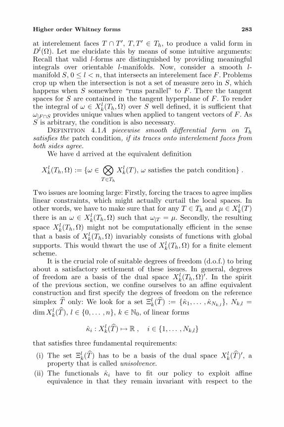
Higher order Whitney forms 283
at interelement faces T ∩ T ′, T, T ′ ∈ Th, to produce a valid form inDl(Ω). Let me elucidate this by means of some intuitive arguments:Recall that valid l-forms are distinguished by providing meaningfulintegrals over orientable l-manifolds. Now, consider a smooth l-manifold S, 0 ≤ l < n, that intersects an interelement face F . Problemscrop up when the intersection is not a set of measure zero in S, whichhappens when S somewhere “runs parallel” to F . There the tangentspaces for S are contained in the tangent hyperplane of F . To renderthe integral of ω ∈ X l
k(Th,Ω) over S well defined, it is sufficient thatω|F∩S provides unique values when applied to tangent vectors of F . AsS is arbitrary, the condition is also necessary.
Definition 4.1A piecewise smooth differential form on Thsatisfies the patch condition, if its traces onto interelement faces fromboth sides agree.
We have d arrived at the equivalent definition
X lk(Th,Ω) := ω ∈
⊗T∈Th
X lk(T ), ω satisfies the patch condition .
Two issues are looming large: Firstly, forcing the traces to agree implieslinear constraints, which might actually curtail the local spaces. Inother words, we have to make sure that for any T ∈ Th and µ ∈ X l
k(T )there is an ω ∈ X l
k(Th,Ω) such that ω|T = µ. Secondly, the resultingspace X l
k(Th,Ω) might not be computationally efficient in the sensethat a basis of X l
k(Th,Ω) invariably consists of functions with globalsupports. This would thwart the use of X l
k(Th,Ω) for a finite elementscheme.
It is the crucial role of suitable degrees of freedom (d.o.f.) to bringabout a satisfactory settlement of these issues. In general, degreesof freedom are a basis of the dual space X l
k(Th,Ω)′. In the spiritof the previous section, we confine ourselves to an affine equivalentconstruction and first specify the degrees of freedom on the referencesimplex T only: We look for a set Ξlk(T ) := κ1, . . . , κNk,l, Nk,l =dimX l
k(T ), l ∈ 0, . . . , n, k ∈ N0, of linear forms
κi : X lk(T ) → R , i ∈ 1, . . . , Nk,l
that satisfies three fundamental requirements:
(i) The set Ξlk(T ) has to be a basis of the dual space X lk(T )′, a
property that is called unisolvence.(ii) The functionals κi have to fit our policy to exploit affine
equivalence in that they remain invariant with respect to the
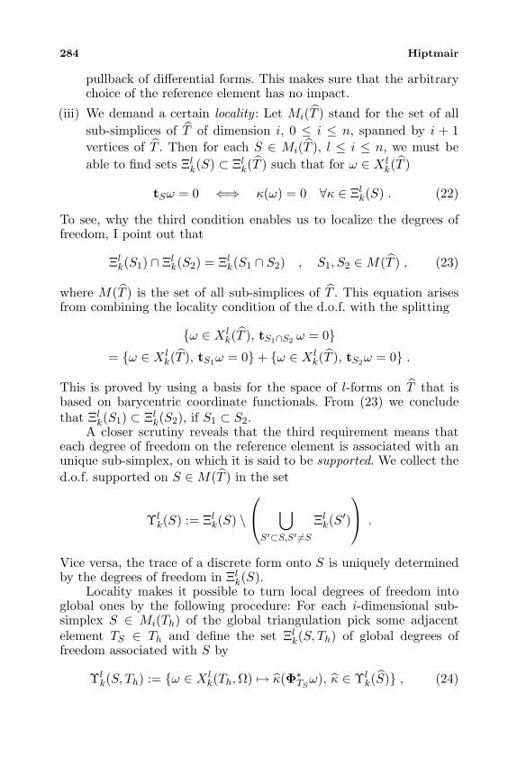
284 Hiptmair
pullback of differential forms. This makes sure that the arbitrarychoice of the reference element has no impact.
(iii) We demand a certain locality : Let Mi(T ) stand for the set of allsub-simplices of T of dimension i, 0 ≤ i ≤ n, spanned by i + 1vertices of T . Then for each S ∈ Mi(T ), l ≤ i ≤ n, we must beable to find sets Ξlk(S) ⊂ Ξlk(T ) such that for ω ∈ X l
k(T )
tSω = 0 ⇐⇒ κ(ω) = 0 ∀κ ∈ Ξlk(S) . (22)
To see, why the third condition enables us to localize the degrees offreedom, I point out that
Ξlk(S1) ∩ Ξlk(S2) = Ξlk(S1 ∩ S2) , S1, S2 ∈M(T ) , (23)
where M(T ) is the set of all sub-simplices of T . This equation arisesfrom combining the locality condition of the d.o.f. with the splitting
ω ∈ X lk(T ), tS1∩S2 ω = 0
= ω ∈ X lk(T ), tS1ω = 0+ ω ∈ X l
k(T ), tS2ω = 0 .
This is proved by using a basis for the space of l-forms on T that isbased on barycentric coordinate functionals. From (23) we concludethat Ξlk(S1) ⊂ Ξlk(S2), if S1 ⊂ S2.
A closer scrutiny reveals that the third requirement means thateach degree of freedom on the reference element is associated with anunique sub-simplex, on which it is said to be supported. We collect thed.o.f. supported on S ∈M(T ) in the set
Υlk(S) := Ξlk(S) \
⋃S′⊂S,S′ =S
Ξlk(S′)
.
Vice versa, the trace of a discrete form onto S is uniquely determinedby the degrees of freedom in Ξlk(S).
Locality makes it possible to turn local degrees of freedom intoglobal ones by the following procedure: For each i-dimensional sub-simplex S ∈ Mi(Th) of the global triangulation pick some adjacentelement TS ∈ Th and define the set Ξlk(S, Th) of global degrees offreedom associated with S by
Υlk(S, Th) := ω ∈ X l
k(Th,Ω) → κ(Φ∗TSω), κ ∈ Υlk(S) , (24)
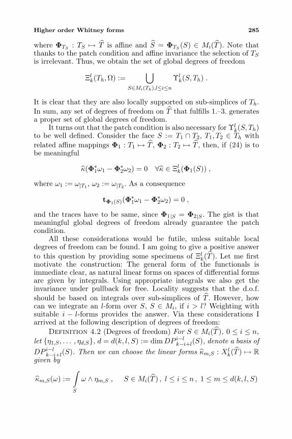
Higher order Whitney forms 285
where ΦTS : TS → T is affine and S = ΦTS (S) ∈ Mi(T ). Note thatthanks to the patch condition and affine invariance the selection of TSis irrelevant. Thus, we obtain the set of global degrees of freedom
Ξlk(Th,Ω) :=⋃
S∈Mi(Th),l≤i≤nΥlk(S, Th) .
It is clear that they are also locally supported on sub-simplices of Th.In sum, any set of degrees of freedom on T that fulfills 1.–3. generatesa proper set of global degrees of freedom.
It turns out that the patch condition is also necessary for Υlk(S, Th)
to be well defined. Consider the face S := T1 ∩ T2, T1, T2 ∈ Th withrelated affine mappings Φ1 : T1 → T , Φ2 : T2 → T , then, if (24) is tobe meaningful
κ(Φ∗1ω1 −Φ∗2ω2) = 0 ∀κ ∈ Ξlk(Φ1(S)) ,
where ω1 := ω|T1, ω2 := ω|T2
. As a consequence
tΦ1(S)(Φ∗1ω1 −Φ∗2ω2) = 0 ,
and the traces have to be same, since Φ1|S = Φ2|S . The gist is thatmeaningful global degrees of freedom already guarantee the patchcondition.
All these considerations would be futile, unless suitable localdegrees of freedom can be found. I am going to give a positive answerto this question by providing some specimens of Ξlk(T ). Let me firstmotivate the construction: The general form of the functionals isimmediate clear, as natural linear forms on spaces of differential formsare given by integrals. Using appropriate integrals we also get theinvariance under pullback for free. Locality suggests that the d.o.f.should be based on integrals over sub-simplices of T . However, howcan we integrate an l-form over S, S ∈ Mi, if i > l? Weighting withsuitable i − l-forms provides the answer. Via these considerations Iarrived at the following description of degrees of freedom:
Definition 4.2 (Degrees of freedom) For S ∈Mi(T ), 0 ≤ i ≤ n,let η1,S , . . . , ηd,S, d = d(k, l, S) := dimDP i−lk−i+l(S), denote a basis ofDP i−lk−i+l(S). Then we can choose the linear forms κm,S : X l
k(T ) → R
given by
κm,S(ω) :=∫S
ω ∧ ηm,S , S ∈Mi(T ) , l ≤ i ≤ n , 1 ≤ m ≤ d(k, l, S)
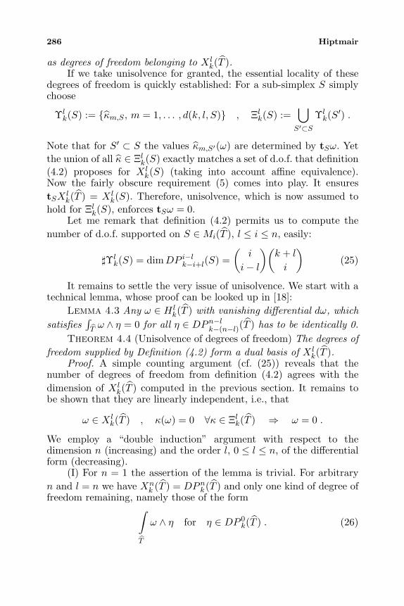
286 Hiptmair
as degrees of freedom belonging to X lk(T ).
If we take unisolvence for granted, the essential locality of thesedegrees of freedom is quickly established: For a sub-simplex S simplychoose
Υlk(S) := κm,S , m = 1, . . . , d(k, l, S) , Ξlk(S) :=
⋃S′⊂S
Υlk(S′) .
Note that for S′ ⊂ S the values κm,S′(ω) are determined by tSω. Yetthe union of all κ ∈ Ξlk(S) exactly matches a set of d.o.f. that definition(4.2) proposes for X l
k(S) (taking into account affine equivalence).Now the fairly obscure requirement (5) comes into play. It ensurestSX l
k(T ) = X lk(S). Therefore, unisolvence, which is now assumed to
hold for Ξlk(S), enforces tSω = 0.Let me remark that definition (4.2) permits us to compute the
number of d.o.f. supported on S ∈Mi(T ), l ≤ i ≤ n, easily:
%Υlk(S) = dimDP i−lk−i+l(S) =
(i
i− l
)(k + l
i
)(25)
It remains to settle the very issue of unisolvence. We start with atechnical lemma, whose proof can be looked up in [18]:
Lemma 4.3 Any ω ∈ H lk(T ) with vanishing differential dω, which
satisfies∫Tω ∧ η = 0 for all η ∈ DPn−lk−(n−l)(T ) has to be identically 0.
Theorem 4.4 (Unisolvence of degrees of freedom) The degrees offreedom supplied by Definition (4.2) form a dual basis of X l
k(T ).Proof. A simple counting argument (cf. (25)) reveals that the
number of degrees of freedom from definition (4.2) agrees with thedimension of X l
k(T ) computed in the previous section. It remains tobe shown that they are linearly independent, i.e., that
ω ∈ X lk(T ) , κ(ω) = 0 ∀κ ∈ Ξlk(T ) ⇒ ω = 0 .
We employ a “double induction” argument with respect to thedimension n (increasing) and the order l, 0 ≤ l ≤ n, of the differentialform (decreasing).
(I) For n = 1 the assertion of the lemma is trivial. For arbitraryn and l = n we have Xn
k (T ) = DPnk(T ) and only one kind of degree offreedom remaining, namely those of the form∫
T
ω ∧ η for η ∈ DP 0k(T ) . (26)
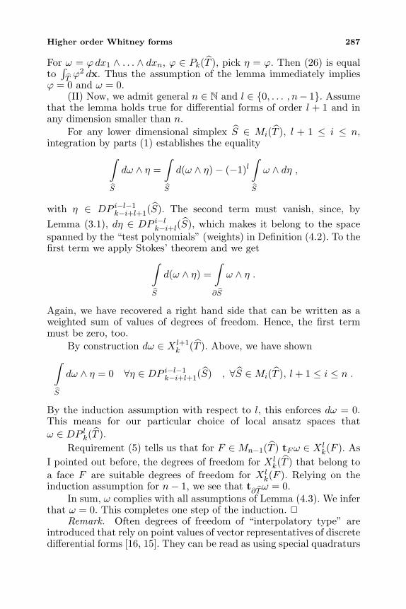
Higher order Whitney forms 287
For ω = ϕdx1 ∧ . . . ∧ dxn, ϕ ∈ Pk(T ), pick η = ϕ. Then (26) is equalto
∫Tϕ2 dx. Thus the assumption of the lemma immediately implies
ϕ = 0 and ω = 0.(II) Now, we admit general n ∈ N and l ∈ 0, . . . , n− 1. Assume
that the lemma holds true for differential forms of order l + 1 and inany dimension smaller than n.
For any lower dimensional simplex S ∈ Mi(T ), l + 1 ≤ i ≤ n,integration by parts (1) establishes the equality
∫
S
dω ∧ η =∫
S
d(ω ∧ η)− (−1)l∫
S
ω ∧ dη ,
with η ∈ DP i−l−1k−i+l+1(S). The second term must vanish, since, by
Lemma (3.1), dη ∈ DP i−lk−i+l(S), which makes it belong to the spacespanned by the “test polynomials” (weights) in Definition (4.2). To thefirst term we apply Stokes’ theorem and we get∫
S
d(ω ∧ η) =∫
∂S
ω ∧ η .
Again, we have recovered a right hand side that can be written as aweighted sum of values of degrees of freedom. Hence, the first termmust be zero, too.
By construction dω ∈ X l+1k (T ). Above, we have shown
∫
S
dω ∧ η = 0 ∀η ∈ DP i−l−1k−i+l+1(S) , ∀S ∈Mi(T ), l + 1 ≤ i ≤ n .
By the induction assumption with respect to l, this enforces dω = 0.This means for our particular choice of local ansatz spaces thatω ∈ DP lk(T ).
Requirement (5) tells us that for F ∈Mn−1(T ) tFω ∈ X lk(F ). As
I pointed out before, the degrees of freedom for X lk(T ) that belong to
a face F are suitable degrees of freedom for X lk(F ). Relying on the
induction assumption for n− 1, we see that t∂Tω = 0.
In sum, ω complies with all assumptions of Lemma (4.3). We inferthat ω = 0. This completes one step of the induction.
Remark. Often degrees of freedom of “interpolatory type” areintroduced that rely on point values of vector representatives of discretedifferential forms [16, 15]. They can be read as using special quadraturs
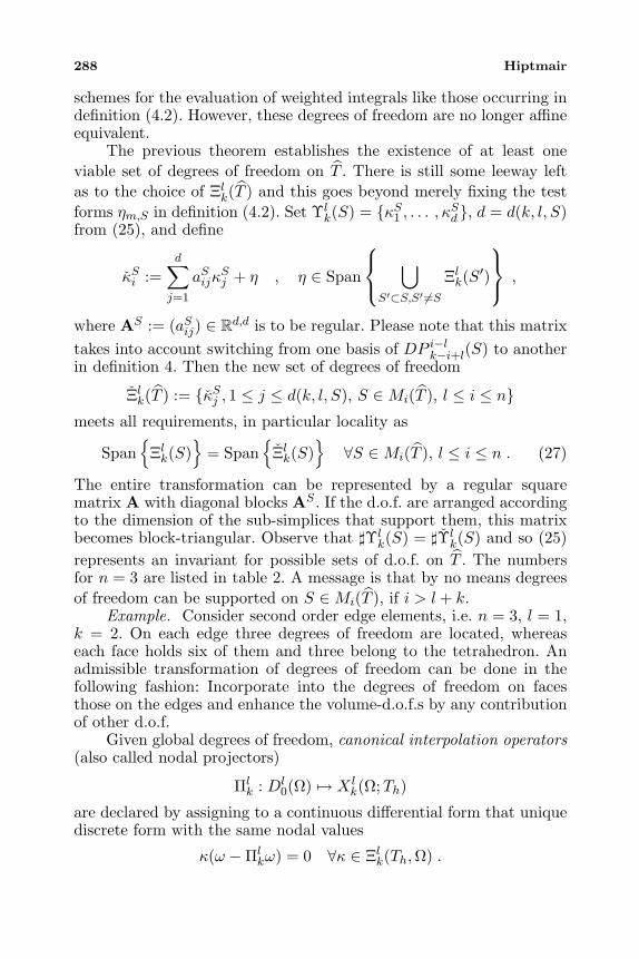
288 Hiptmair
schemes for the evaluation of weighted integrals like those occurring indefinition (4.2). However, these degrees of freedom are no longer affineequivalent.
The previous theorem establishes the existence of at least oneviable set of degrees of freedom on T . There is still some leeway leftas to the choice of Ξlk(T ) and this goes beyond merely fixing the testforms ηm,S in definition (4.2). Set Υl
k(S) = κS1 , . . . , κSd , d = d(k, l, S)from (25), and define
κSi :=d∑j=1
aSijκSj + η , η ∈ Span
⋃S′⊂S,S′ =S
Ξlk(S′)
,
where AS := (aSij) ∈ Rd,d is to be regular. Please note that this matrixtakes into account switching from one basis of DP i−lk−i+l(S) to anotherin definition 4. Then the new set of degrees of freedom
Ξlk(T ) := κSj , 1 ≤ j ≤ d(k, l, S), S ∈Mi(T ), l ≤ i ≤ nmeets all requirements, in particular locality as
Span
Ξlk(S)
= Span
Ξlk(S)∀S ∈Mi(T ), l ≤ i ≤ n . (27)
The entire transformation can be represented by a regular squarematrix A with diagonal blocks AS . If the d.o.f. are arranged accordingto the dimension of the sub-simplices that support them, this matrixbecomes block-triangular. Observe that %Υl
k(S) = %Υlk(S) and so (25)
represents an invariant for possible sets of d.o.f. on T . The numbersfor n = 3 are listed in table 2. A message is that by no means degreesof freedom can be supported on S ∈Mi(T ), if i > l + k.
Example. Consider second order edge elements, i.e. n = 3, l = 1,k = 2. On each edge three degrees of freedom are located, whereaseach face holds six of them and three belong to the tetrahedron. Anadmissible transformation of degrees of freedom can be done in thefollowing fashion: Incorporate into the degrees of freedom on facesthose on the edges and enhance the volume-d.o.f.s by any contributionof other d.o.f.
Given global degrees of freedom, canonical interpolation operators(also called nodal projectors)
Πlk : Dl
0(Ω) → X lk(Ω;Th)
are declared by assigning to a continuous differential form that uniquediscrete form with the same nodal values
κ(ω −Πlkω) = 0 ∀κ ∈ Ξlk(Th,Ω) .
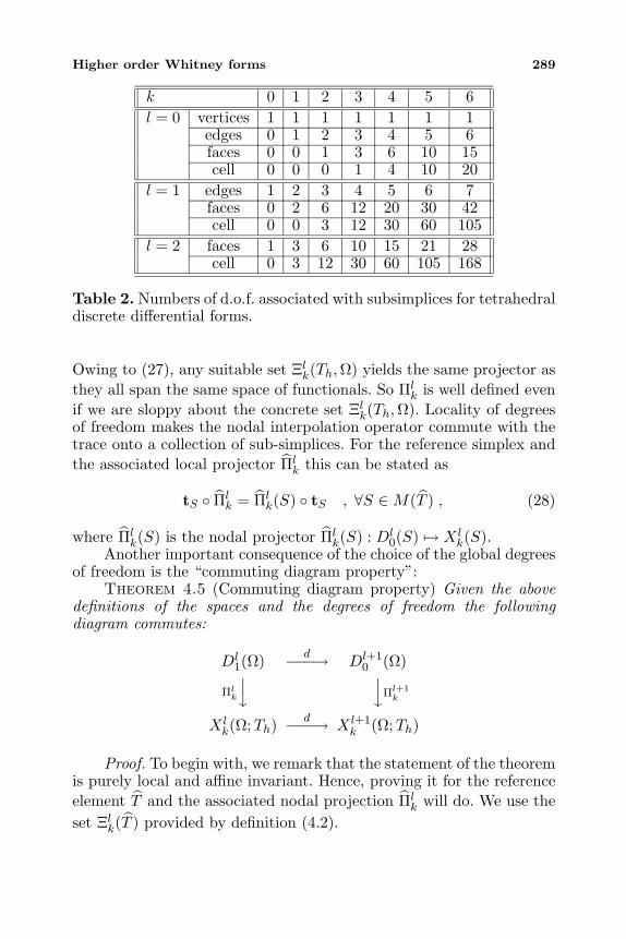
Higher order Whitney forms 289
k 0 1 2 3 4 5 6l = 0 vertices 1 1 1 1 1 1 1
edges 0 1 2 3 4 5 6faces 0 0 1 3 6 10 15cell 0 0 0 1 4 10 20
l = 1 edges 1 2 3 4 5 6 7faces 0 2 6 12 20 30 42cell 0 0 3 12 30 60 105
l = 2 faces 1 3 6 10 15 21 28cell 0 3 12 30 60 105 168
Table 2. Numbers of d.o.f. associated with subsimplices for tetrahedraldiscrete differential forms.
Owing to (27), any suitable set Ξlk(Th,Ω) yields the same projector asthey all span the same space of functionals. So Πl
k is well defined evenif we are sloppy about the concrete set Ξlk(Th,Ω). Locality of degreesof freedom makes the nodal interpolation operator commute with thetrace onto a collection of sub-simplices. For the reference simplex andthe associated local projector Πl
k this can be stated as
tS Πlk = Πl
k(S) tS , ∀S ∈M(T ) , (28)
where Πlk(S) is the nodal projector Πl
k(S) : Dl0(S) → X l
k(S).Another important consequence of the choice of the global degrees
of freedom is the “commuting diagram property”:Theorem 4.5 (Commuting diagram property) Given the above
definitions of the spaces and the degrees of freedom the followingdiagram commutes:
Dl1(Ω) d−−−→ Dl+1
0 (Ω)
Πlk
##Πl+1
k
X lk(Ω;Th)
d−−−→ X l+1k (Ω;Th)
Proof. To begin with, we remark that the statement of the theoremis purely local and affine invariant. Hence, proving it for the referenceelement T and the associated nodal projection Πl
k will do. We use theset Ξlk(T ) provided by definition (4.2).
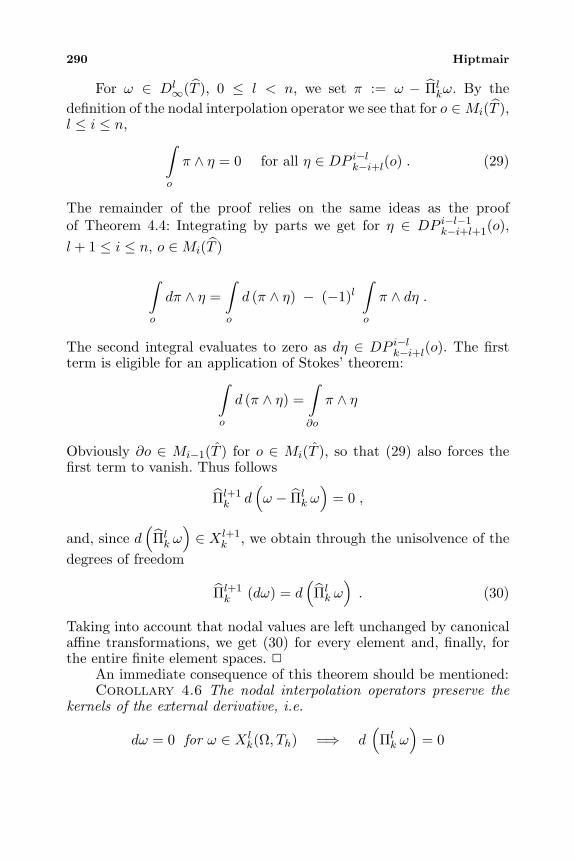
290 Hiptmair
For ω ∈ Dl∞(T ), 0 ≤ l < n, we set π := ω − Πl
kω. By thedefinition of the nodal interpolation operator we see that for o ∈Mi(T ),l ≤ i ≤ n, ∫
o
π ∧ η = 0 for all η ∈ DP i−lk−i+l(o) . (29)
The remainder of the proof relies on the same ideas as the proofof Theorem 4.4: Integrating by parts we get for η ∈ DP i−l−1
k−i+l+1(o),l + 1 ≤ i ≤ n, o ∈Mi(T )
∫o
dπ ∧ η =∫o
d (π ∧ η) − (−1)l∫o
π ∧ dη .
The second integral evaluates to zero as dη ∈ DP i−lk−i+l(o). The firstterm is eligible for an application of Stokes’ theorem:∫
o
d (π ∧ η) =∫∂o
π ∧ η
Obviously ∂o ∈ Mi−1(T ) for o ∈ Mi(T ), so that (29) also forces thefirst term to vanish. Thus follows
Πl+1k d
(ω − Πl
k ω)
= 0 ,
and, since d(Πlk ω
)∈ X l+1
k , we obtain through the unisolvence of thedegrees of freedom
Πl+1k (dω) = d
(Πlk ω
). (30)
Taking into account that nodal values are left unchanged by canonicalaffine transformations, we get (30) for every element and, finally, forthe entire finite element spaces.
An immediate consequence of this theorem should be mentioned:Corollary 4.6 The nodal interpolation operators preserve the
kernels of the external derivative, i.e.
dω = 0 for ω ∈ X lk(Ω, Th) =⇒ d
(Πlk ω
)= 0
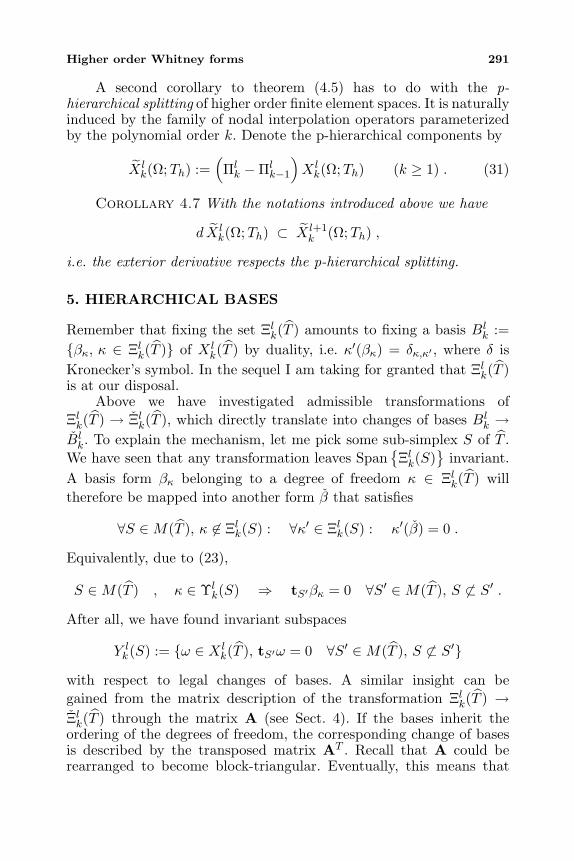
Higher order Whitney forms 291
A second corollary to theorem (4.5) has to do with the p-hierarchical splitting of higher order finite element spaces. It is naturallyinduced by the family of nodal interpolation operators parameterizedby the polynomial order k. Denote the p-hierarchical components by
X lk(Ω;Th) :=
(Πlk −Πl
k−1
)X lk(Ω;Th) (k ≥ 1) . (31)
Corollary 4.7 With the notations introduced above we have
d X lk(Ω;Th) ⊂ X l+1
k (Ω;Th) ,
i.e. the exterior derivative respects the p-hierarchical splitting.
5. HIERARCHICAL BASES
Remember that fixing the set Ξlk(T ) amounts to fixing a basis Blk :=
βκ, κ ∈ Ξlk(T ) of X lk(T ) by duality, i.e. κ′(βκ) = δκ,κ′ , where δ is
Kronecker’s symbol. In the sequel I am taking for granted that Ξlk(T )is at our disposal.
Above we have investigated admissible transformations ofΞlk(T ) → Ξlk(T ), which directly translate into changes of bases Bl
k →Blk. To explain the mechanism, let me pick some sub-simplex S of T .
We have seen that any transformation leaves SpanΞlk(S)
invariant.
A basis form βκ belonging to a degree of freedom κ ∈ Ξlk(T ) willtherefore be mapped into another form β that satisfies
∀S ∈M(T ), κ ∈ Ξlk(S) : ∀κ′ ∈ Ξlk(S) : κ′(β) = 0 .
Equivalently, due to (23),
S ∈M(T ) , κ ∈ Υlk(S) ⇒ tS′βκ = 0 ∀S′ ∈M(T ), S ⊂ S′ .
After all, we have found invariant subspaces
Y lk(S) := ω ∈ X l
k(T ), tS′ω = 0 ∀S′ ∈M(T ), S ⊂ S′
with respect to legal changes of bases. A similar insight can begained from the matrix description of the transformation Ξlk(T ) →Ξlk(T ) through the matrix A (see Sect. 4). If the bases inherit theordering of the degrees of freedom, the corresponding change of basesis described by the transposed matrix AT . Recall that A could berearranged to become block-triangular. Eventually, this means that
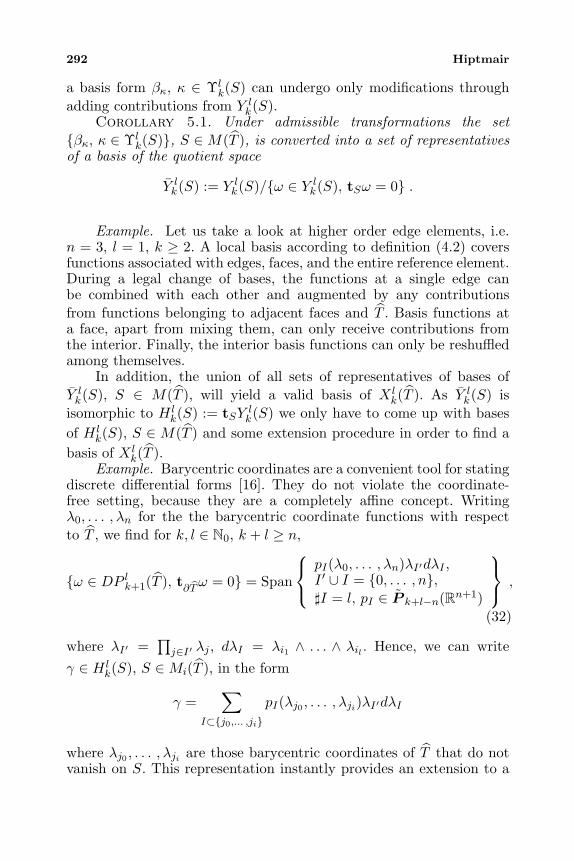
292 Hiptmair
a basis form βκ, κ ∈ Υlk(S) can undergo only modifications through
adding contributions from Y lk(S).
Corollary 5.1. Under admissible transformations the setβκ, κ ∈ Υl
k(S), S ∈M(T ), is converted into a set of representativesof a basis of the quotient space
Y lk(S) := Y l
k(S)/ω ∈ Y lk(S), tSω = 0 .
Example. Let us take a look at higher order edge elements, i.e.n = 3, l = 1, k ≥ 2. A local basis according to definition (4.2) coversfunctions associated with edges, faces, and the entire reference element.During a legal change of bases, the functions at a single edge canbe combined with each other and augmented by any contributionsfrom functions belonging to adjacent faces and T . Basis functions ata face, apart from mixing them, can only receive contributions fromthe interior. Finally, the interior basis functions can only be reshuffledamong themselves.
In addition, the union of all sets of representatives of bases ofY lk(S), S ∈ M(T ), will yield a valid basis of X l
k(T ). As Y lk(S) is
isomorphic to H lk(S) := tSY l
k(S) we only have to come up with basesof H l
k(S), S ∈ M(T ) and some extension procedure in order to find abasis of X l
k(T ).Example. Barycentric coordinates are a convenient tool for stating
discrete differential forms [16]. They do not violate the coordinate-free setting, because they are a completely affine concept. Writingλ0, . . . , λn for the the barycentric coordinate functions with respectto T , we find for k, l ∈ N0, k + l ≥ n,
ω ∈ DP lk+1(T ), t∂Tω = 0 = Span
pI(λ0, . . . , λn)λI′dλI ,I ′ ∪ I = 0, . . . , n,%I = l, pI ∈ P k+l−n(Rn+1)
,
(32)
where λI′ =∏j∈I′ λj , dλI = λi1 ∧ . . . ∧ λil . Hence, we can write
γ ∈ H lk(S), S ∈Mi(T ), in the form
γ =∑
I⊂j0,... ,jipI(λj0 , . . . , λji)λI′dλI
where λj0 , . . . , λji are those barycentric coordinates of T that do notvanish on S. This representation instantly provides an extension to a
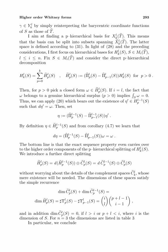
Higher order Whitney forms 293
γ ∈ Y lk by simply reinterpreting the barycentric coordinate functions
of S as those of T .I aim at finding a p–hierarchical basis for X l
k(T ). This meansthat the basis can be split into subsets spanning X l
k(T ). The latterspace is defined according to (31). In light of (28) and the precedingconsiderations, I first focus on hierarchical bases forH l
k(S), S ∈Mi(T ),l ≤ i ≤ n. Fix S ∈ Mi(T ) and consider the direct p–hierarchicaldecomposition
H lk(S) =
k∑p=0
H lp(S) , H l
p(S) := (Πlp(S)− Πl
p−1(S))H lk(S) for p > 0 .
Then, for p > 0 pick a closed form ω ∈ H lp(S). If i = l, the fact that
ω belongs to a genuine hierarchical surplus (p > 0) implies∫S ω = 0.
Thus, we can apply (20) which bears out the existence of η′ ∈ H l−1p (S)
such that dη′ = ω. Then, set
η := (Πl−1p (S)− Πl−1
p−1(S))η′ .
By definition η ∈ H l−1p (S) and from corollary (4.7) we learn that
dη = (Πl−1p (S)− Πl
p−1(S))ω = ω .
The bottom line is that the exact sequence property even carries overto the higher order components of the p–hierarchical splitting ofH l
k(S).We introduce a further direct splitting
H lp(S) = d(H l−1
p (S))⊕ C lp(S) = d C l−1p (S)⊕ C lp(S)
without worrying about the details of the complement spaces C lk, whosemere existence will be needed. The dimensions of these spaces satisfythe simple recurrence
dim C lp(S) + dim C l−1p (S) =
dim H lp(S) = %Υl
p(S)− %Υlp−1(S) =
(i
l
)(p+ l − 1i− 1
),
and in addition dim C lp(S) = 0, if l > i or p + l < i, where i is thedimension of S. For n = 3 the dimensions are listed in table 3
In particular, we conclude
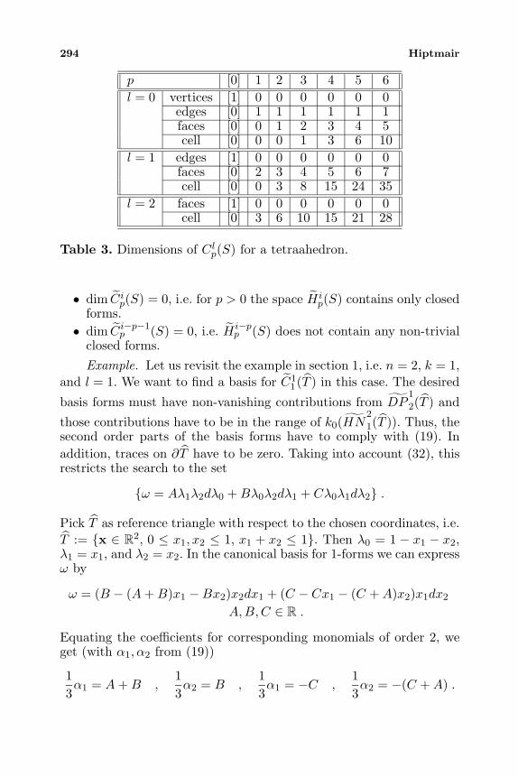
294 Hiptmair
p [0] 1 2 3 4 5 6l = 0 vertices [1] 0 0 0 0 0 0
edges [0] 1 1 1 1 1 1faces [0] 0 1 2 3 4 5cell [0] 0 0 1 3 6 10
l = 1 edges [1] 0 0 0 0 0 0faces [0] 2 3 4 5 6 7cell [0] 0 3 8 15 24 35
l = 2 faces [1] 0 0 0 0 0 0cell [0] 3 6 10 15 21 28
Table 3. Dimensions of C lp(S) for a tetraahedron.
• dim Cip(S) = 0, i.e. for p > 0 the space H ip(S) contains only closed
forms.• dim Ci−p−1
p (S) = 0, i.e. H i−pp (S) does not contain any non-trivial
closed forms.Example. Let us revisit the example in section 1, i.e. n = 2, k = 1,
and l = 1. We want to find a basis for C11 (T ) in this case. The desired
basis forms must have non-vanishing contributions from DP1
2(T ) and
those contributions have to be in the range of k0(HN2
1(T )). Thus, thesecond order parts of the basis forms have to comply with (19). Inaddition, traces on ∂T have to be zero. Taking into account (32), thisrestricts the search to the set
ω = Aλ1λ2dλ0 +Bλ0λ2dλ1 + Cλ0λ1dλ2 .
Pick T as reference triangle with respect to the chosen coordinates, i.e.T := x ∈ R2, 0 ≤ x1, x2 ≤ 1, x1 + x2 ≤ 1. Then λ0 = 1 − x1 − x2,λ1 = x1, and λ2 = x2. In the canonical basis for 1-forms we can expressω by
ω = (B − (A+B)x1 −Bx2)x2dx1 + (C − Cx1 − (C +A)x2)x1dx2
A,B,C ∈ R .
Equating the coefficients for corresponding monomials of order 2, weget (with α1, α2 from (19))
13α1 = A+B ,
13α2 = B ,
13α1 = −C ,
13α2 = −(C +A) .
Higher order Whitney forms 295
A solution exists for any α1, α2 ∈ R, e.g. α1 = 3, α2 = 0 leadsto A = 1, B = 0, C = −1, whereas α1 = 0, α2 = 3 meansA = 1, B = −1, C = 0. Then we arrive at the following two basisforms for C1
1 (T )
β1 = −x1x2dx1 + (x1 − 1)x1dx2 , β2 = (1− x2)x2dx1 − x2x1dx2 .
Here no hierarchical surplus has to be computed, as there are no non-trivial discrete 1-forms of order 0 that are supported in the interior ofa triangle.
To continue with the construction of hierarchical bases, we selectbases ζ l,Sp,1 , . . . , ζ
l,Sp,K, K = K(l, p, S) := dim C lp(S), of C lp(S). The
freedom at this stage will mean that many different instances of p-hierarchical bases are possible. Since H l
k(S) := tSY lk(S) these basis
forms can be extended to forms γl,Sp,1, . . . , γl,Sp,K in Y l
k(S). Finally set
βl,Sp,j := (Πlp − Πl
p−1)γl,Sp,j , 1 ≤ j ≤ K .
As Y lk(S) is invariant under the nodal projectors Πl
p, 0 ≤ p ≤ k, the βl,Sp,jstill belong to Y l
k(S). Thanks to (28) we know tSβl,Sp,j = ζ l,Sp,j . In sum,
βl,Sp,1, . . . , βl,Sp,K are representatives of linearly independent elements of
Y lk(S) and they respect the hierarchical decomposition.
Now we are in a position to describe the hierarchical bases forX lk(T ) explicitly through
Bl0 ∪
βl,Sp,j , dβ
l,Sp,m, 1 ≤ j ≤ K(l, p, S), 1 ≤ m ≤ K(l − 1, p, S),
S ∈Mi(T ), 0 ≤ i ≤ n, 1 ≤ p ≤ k
.
(33)
Linear independence of the forms is clear from the way theyhave been constructed. As well, their construction guarantees thelocality property. However, can any ω ∈ X l
k(T ) be expressed as alinear combination of forms from (33)? Start with the p–hierarchicaldecomposition of ω
ω = ω0 + . . .+ ωk , ω0 := Πl0ω , ωp := (Πl
p − Πlp−1)ω, 0 ≤ p ≤ k .
Then pick S ∈ Ml(T ) and express tSωp ∈ X lp(S) through
ζ l,Sp,1 , . . . , ζl,SK,p, dζ
l−1,Sp,1 , . . . , dζ l−1,S
M,p . Subtracting the same linear
combination of βl,Sp,1, . . . , βl,Sp,K , dβ
l−1,Sp,1 , . . . , dβl−1,S
p,M from ωp yields
296 Hiptmair
ω′p ∈ X lp(T ) with vanishing trace on S. Carrying out the same
procedure for the other sub-simplices in Ml(T ) results in a formω ∈ X l
p(T ) whose trace on all l-dimensional subsimplices is zero.Choosing S ∈ Ml+1(T ) this means tSω ∈ H l
p(S) and we can repeatthe construction for l+ 1-dimensional sub-simplices. This can be doneuntil we reach S = T . I point out that a closed ωp, p ≥ 1, willfinally be represented solely through closed basis forms. This shouldbe remembered as an interesting feature of (33).
As the hierarchical basis (33) complies with all requirements,it induces valid local degrees of freedom and, thus, a correspondingbasis of the global space X l
k(Th,Ω). The global basis retains all affine-invariant, say all essential, features of the local hierarchical basis ofX lk(T ):
Theorem 5.2 Given a closed discrete differential form in thehierarchical surplus space X l
p(Th,Ω), p ≥ 1, it can be written as linearcombination of closed forms with local support.
Proof Everything has already been settled by the aboveconsiderations. The local contributions are spawned by exteriorderivatives of hierarchical basis functions for discrete l − 1-forms.
Remark. Recursion lends itself for the practical construction ofthe hierarchical basis: Build hierarchical bases H l
k(T ) for in dimensionsl, . . . , n−1 first. Then extend them to elements of the hierarchical basisof X l
k(T ). Extension is straightforward, if barycentric coordinates areused to represent the differential forms.
The hierarchical basis is also the key to building spaces of discretedifferential forms on Th, whose polynomial degree may vary fromelement to element. For each T ∈ Th we fix pT ∈ N0, which standsfor the desired polynomial degree on that particular element. Thendefine
pS := minpT , S ⊂ T , S ∈M(Th) . (34)
as the polynomial degree associated with each sub-simplex S of themesh. As is the case with any admissible basis, the forms in the globalhierarchical basis of X l
k(Th,Ω) belong to exactly one sub-simplex ofTh. The global p–adaptive basis is then given by
BlpT :=
⋃S∈M(Th)
Basis l-forms of degree ≤ pS associated with S .
Of course, the global p–adaptive space of discrete l-forms is defined as
X lpT (Ω, Th) := Span
BlpT
.
Higher order Whitney forms 297
Theorem 5.3 If Ω is contractible, the spaces X lpT (Ω, Th), 0 ≤
l ≤ n, possess the exact sequence property.Proof. If ω ∈ X l
pT (Ω, Th) is closed we can split it into two closedforms according to
ω = ω0 + ω, ω0 = Πl0 .
As seen before, the hierarchical surplus ω can only comprise closed basisforms of Bl
pT that are derivatives of hierarchical basis l − 1-forms ofthe same polynomial degree and belonging to the same sub-simplex:
∃η ∈ X l−1pT (Ω, Th) : ω = dη .
The existence of a discrete potential for lowest order discretedifferential forms (Whitney-forms) is a result from topology.
Remark. It turns out that the existence of discrete potentials iscrucial for the discrete compactness property of edge elements (discrete1-forms) [21, 10, 5]. Discrete compactness is a necessary conditionfor the convergence of Galerkin finite element solutions of eigenvalueproblems.
Of course, BlpT (Ω, Th) is not the only possible basis for X l
pT and there is ample room for better choices following the prescriptionsfrom the beginning of the paragraph. For finite element applicationschanging to another basis is even recommended in order to improvethe condition number of the resulting system of linear equations [2].
REFERENCES
1. Andersen, L. and J. Volakis, “Development and application ofa novel class of hierarchical tangential vector finite elementsfor electromagnetics,” IEEE Trans. Antennas and Propagation,Vol. 47, 112–120, 1999.
2. Babuska, I., M. Griebel, and J. Pitkaranta, “The problem ofselecting the shape functions for a p-type finite element,” Int. J.Num. Meth. Engin., Vol. 28, 1891–1908, 1988.
3. Baldomir, D. and P. Hammond, Geometry of ElectromagneticSystems, Clarendon Press, Oxford, 1996.
4. Beck, R., R. Hiptmair, and B. Wohlmuth, “A hierarchicalerror estimator for eddy current computation,” ENUMATH 99— Proceedings of the 3rd European Conference on NumericalMathematics and Advanced Applications, P. Neittaanmaki andT. Tiihonen (eds.), July 26–30, Jyvskyl, Finland, 110–120, WorldScientific, Singapore, 2000.
298 Hiptmair
5. Boffi, D., “Discrete compactness and Fortin operator for edgeelements,” Tech. Rep. AM187, Department of Mathematics,Pennsylvania State University, State College, USA, April 1999.To appear in Numerische Mathematik.
6. Bossavit, A., “Mixed finite elements and the complex of Whitneyforms,” The Mathematics of Finite Elements and Applications VI,J. Whiteman (ed.), 137–144, Academic Press, London, 1988.
7. Bossavit, A., “Whitney forms: A class of finite elements for three-dimensional computations in electromagnetism,” IEE Proc. A,Vol. 135, 493–500, 1988.
8. Bossavit, A., “On the geometry of electromagnetism IV:“Maxwell’s house,” J. Japan Soc. Appl. Electromagnetics &Mech., Vol. 6,318–326, 1998.
9. Brenner, S. and R. Scott, Mathematical Theory of Finite ElementMethods, Texts in Applied Mathematics, Springer-Verlag, NewYork, 1994.
10. Caorsi, S., P. Fernandes, and M. Raffetto, “On the convergenceof Galerkin finite element approximations of electromagneticeigenproblems,” SIAM J. Numer. Anal., To appear.
11. Cartan, H., Formes Differentielles, Hermann, Paris, 1967.12. Ciarlet, P., “The finite element method for elliptic problems,”
Studies in Mathematics and its Applications, Vol. 4, North-Holland, Amsterdam, 1978.
13. Demkowicz, L., P. Monk, L. Vardapetyan, and W. Rachowicz, “DeRham diagram for hp finite element spaces,” Tech. Rep., 99-06,TICAM, University of Texas, Austin, TX, 1999.
14. Deschamps, G., “Electromagnetics and differential forms,” Proc.IEEE, Vol. 69, 676–695, 1981.
15. Elmkies, A. and P. Joly, “Elements finis et condensation de massepour les equations des Maxwell: le cas 3D,” Tech. Rep., 3381,INRIA, Roucquencourt, Domaine de Voluveau, France, May 1998.
16. Graglia, R., D. Wilton, and A. Peterson, “Higher orderinterpolatory vector bases for computational electromagnetics,”IEEE Trans. Antennas and Propagation, Vol. 45, 329–342, 1997.
17. Graglia, R., D. Wilton, A. Peterson, and I.-L. Gheorma, “Higherorder interpolatory vector bases on prism elements,” IEEE Trans.Antennas and Propagation, Vol. 46, 442–450, 1998.
18. Hiptmair, R., “Canonical construction of finite elements,” Math.Comp., Vol. 68,1325–1346, 1999.
19. Iwaniec, T., “Nonlinear differential forms,” “Lectures notes of theInternational Summer School in Jyvaskyla,” 1998 80, University of
Higher order Whitney forms 299
Jyvaskyla, Department of Mathematics, Jyvaskyla, Finland, 1999.20. Monk, P., “On the p and hp-extension of Nedelec’s conforming
elements,” J. Comp. Appl. Math., Vol. 53, 117–137, 1994.21. Monk, P. and L. Demkowicz, “Discrete compactness and the
approximation of Maxwell’s equations in R3,” Math. Comp., 1999,to appear.
22. Nedelec, J., “Mixed finite elements in R3,” Numer. Math., Vol. 35,315–341, 1980.
23. Nedelec, J., “A new family of mixed finite elements in R3,” Numer.Math., Vol. 50, 57–81, 1986.
24. Peng, G., R. Dyczij-Edlinger, and J.-F. Lee, “Hierarchicalmethods for solving matrix equations from TVFEMs formicrowave components,” IEEE Trans. Mag., Vol. 35, 1474–1477,1998.
25. Raviart, P. A. and J. M. Thomas, “A mixed finite element methodfor second order elliptic problems,” Springer Lecture Notes inMathematics, Vol. 606, 292–315, Springer-Verlag, New York, 1977.
26. Savage, J. and A. Peterson, “Higher order vector finite elementsfor tetrahedral cells,” IEEE Trans. Microwave Theory andTechniques, Vol. 44, 874–879, 1996.
27. Whitney, H., Geometric Integration Theory, Princeton Univ.Press, Princeton, 1957.
28. Yiailtsis, T. and T. Tsiboukis, “A systematic approach tothe construction of higher order vector finite elements forthree-dimensional electromagnetic field computation,” COMPEL,Vol. 14, 49–53, 1995.
Progress In Electromagnetics Research, PIER 32, 301–316, 2001
CONSERVATION OF DISCRETE ENERGY ANDRELATED LAWS IN THE FINITE INTEGRATIONTECHNIQUE
R. Schuhmann and T. Weiland
Darmstadt University of Technology, TEMFSchlossgartenstr. 8, 64289 Darmstadt, Germany
Abstract—We report some properties of the Finite IntegrationTechnique (FIT), which are related to the definition of a discrete energyquantity. Starting with the well-known identities for the operatormatrices of the FIT, not only the conservation of discrete energyin time and frequency domain simulations is derived, but also someimportant orthogonality properties for eigenmodes in cavities andwaveguides. Algebraic proofs are presented, which follow the vector-analytical proofs of the related theorems of the classical (continuous)theory. Thus, the discretization approach of the FIT can be consideredas the framework for a consistent discrete electromagnetic field theory.
1 Introduction
2 Orthogonality Properties and Discrete Energy
3 Energy Conservation in the Discrete System
4 Orthogonality of Discrete Waveguide Modes
5 Conclusion
References
1. INTRODUCTION
One of the key points of the Finite Integration Technique [1, 2] isthe use of a system of two computational grids, the primary grid G
and the dual grid G. In the simplest case these are Cartesian-typecoordinate grids (sometimes referred to as Yee-type grids [3]), but alarge variety of more general grids are allowed, such as cylindrical orspherical coordinate grids, triangular [4] or non-orthogonal grids [5].
302 Schuhmann and Weiland
As state variables of the FIT we introduce electric and magneticgrid voltages and fluxes, which are defined as the integrals of theelectric and magnetic field vectors over elementary objects of thecomputational grid: Grid voltages
e i =
∫Li
E(r, t) · ds,
Hj =∫
Lj
H(r, t) · ds, (1)
and grid fluxes
di =
∫
Ai
D(r, t) · d A,b j =
∫Aj
B(r, t) · d A,j i =
∫
Ai
J(r, t) · d A,
(2)
where Li, Aj are the edges and facets of the primary grid G, and Lj , Ai
denote the edges and facets of the dual grid G. The indices are chosensuch, that the primary facet Aj has the same index as the intersectingedge Lj of the dual grid (same to Ai and Li).
Using these definitions, Maxwell’s equations can be transformedinto a set of matrix-vector-equations for the algebraic vectors e ,
d,
h,b, and
j
Ce = − d
dt
b, C
h =d
dt
d +
j , (3)
Sb = 0, S
d = q, (4)
which are referred to as Maxwell’s Grid Equations.The matrix C is the discrete curl-operator of the grid G: Its entries
Cji are ±1, only if edge Li is contained in the boundary of facet Aj ,and zero otherwise (incidence relation). Analogously, the matrix S isthe discrete div-operator1 of the primary grid: Its entries Skj are ±1,only if facet Aj is contained in the boundary of cell k. The same appliesto the matrices S and C and the dual grid G.
From grid topology we find the relations
SC = 0 and SC = 0, (5)
which in the light of the FIT have some important consequences: Asdirect analogs to the vector-analytical identity ‘div rot=0’ they ensure,1 For historical reasons the div-operators are denoted with S and S (’source’), and symbolsbeginning with D are used for diagonal matrices.
Conservation laws in the finite integration technique 303
that also in the discrete regime we can identify curl-free (solenoidal)and divergence-free fields, and a curl-field is always free of sources. Thisproperty holds exactly (up to numerical round-off) for all discrete fieldvectors of the FI-approach (and not only for vanishing grid step sizes∆→ 0).
Another topological result is the duality of the curl-operators
C = CT , (6)
which plays an important role in the following analysis of the discreteeigenvalue problem of the FIT. Furthermore, the transposed matrix ofthe div-operator ST can be identified to be the negative dual gradient:
G = −ST and G = −ST . (7)
In the case of a Cartesian grid system with NP primary nodeswe can choose the indexing of the edges and facets such, that in thediscrete vectors the x−, y− and z−components are separated,
e =
exeyez
,
h =
hxhyhz
. (8)
As a consequence, we obtain NP × NP -blocks Px, Py and Pz in theoperator matrices
C =
( 0 −Pz Py
Pz 0 −Px
−Py Px 0
), C =
0 PT
z −PTy
−PTz 0 PT
x
PTy −PT
x 0
,
(9)
and
S = ( Px Py Pz ) , S =(−PT
x −PTy −PT
z
), (10)
which can be identified as discrete partial differentiation operators[1, 2].
To complete the discretization approach we introduce so-calledmaterial matrices as an analog of the constitutive relations ofcontinuous fields (without polarization vectors):
d = Mε
ej = Mκ
e
h = Mµ−1
b (11)
If we assume a dual-orthogonal grid system, where primary edges anddual facets (or dual edges and primary facets) intersect with an angle
304 Schuhmann and Weiland
of 90 degrees, the material matrices (11) can be defined as diagonalmatrices with the entries
Mε,ii =εAi
Li, Mκ,ii =
κAi
Li, Mµ−1,jj =
LjµAj
, (12)
where ε, κ and µ are properly averaged material coefficients. Theconsistency of these expressions with the continuous relations can beproven by simple Taylor expansions [2, 6].
Obviously, for positive permittivities and permeabilities thematrices Mε and Mµ−1 are symmetric positive definite. This propertytogether with the duality (6) of the curl-operators can be exploited toderive a number of important theorems for the discretization approachof the FIT. This includes the conservation of energy in simulationswith time-varying fields, and various orthogonality relations for theeigensolutions of the method. In the following chapters we firstintroduce the underlying concept of electric and magnetic energy inthe discrete system, and then present some important consequences ofthis definitions and their algebraic proofs.
2. ORTHOGONALITY PROPERTIES AND DISCRETEENERGY
For the rest of this paper we restrict our analysis to Cartesiangrids, as they allow a simple but important definition of a discreteenergy quantity. To motivate the following derivation, we regardthe eigenvalue equation for the electric field in a lossless system (nocurrents)
ε−1curl µ−1curl E = ω2 E (continuous), (13)
M−1ε CTMµ−1C e = ω2 e (discrete), (14)
where the dual curl operator in the discrete formulation was replacedby C = CT according to (6). As the material matrices are diagonaland positive definite, we can define their real-valued ’roots’
Mε = M1/2ε M1/2
ε Mµ−1 = M1/2µ−1 M1/2
µ−1 (15)
by taking the square root of each entry. The system matrix A =M−1
ε CTMµ−1C of the algebraic eigenvalue problem can then besymmetrized by the transformation
e ′ = M1/2ε
e , (16)
Conservation laws in the finite integration technique 305
leading to
M−1/2ε CTMµ−1CM−1/2
εe ′ = ω2 e ′, (17)
with the symmetric positive semidefinite system matrix
A′ = M−1/2ε CTMµ−1CM−1/2
ε = (M1/2µ−1CM−1/2
ε )T (M1/2µ−1CM−1/2
ε ).(18)
Thus all eigenvalues λ = ω2 of equations (14) and (17) are real-valued and non-negative numbers, and all eigensolutions representeither static solutions (with ω = 0) or undamped oscillations withreal eigenfrequencies ω > 0. This is discussed in more detail in [2, 6].
Another important property of eigenvalue problems with apositive definite system matrix is the orthogonality of the modes: Foreach pair of eigenvectors with different eigenvalues we have
(e ′ξ)H e ′η = 0 (λξ = λη). (19)
Re-substituting the original vectors applying (16), we cannormalize the eigenmodes to get
eHξ Mεeη = eHξ
dη =
0 (ξ = η)
1 Watt (ξ = η). (20)
From the physical dimension of the scalar product [eHξdξ] = 1 Watt
it can be identified as an energy-related form, and this motivates thedefinitions of the (time-averaged) total stored electric and magneticdiscrete energy:
W e =14eH
d, Wm =
14
hHb. (21)
For an interpretation of these formulas we consider two (real-valued) components
e i andDi, which refer to a primary grid edge Li
in x-direction, and to the corresponding dual facet Ai. According toFig. 1 this facet consists of four parts ∆Ak (k = 1 . . . 4) with eventuallydifferent permittivities εk.
Based on the (continuous) Ex-component of the electric field atthe intersection point, the first order approximations
e i ≈ Ex · Li,
di ≈ Ex ·
4∑k=1
εk ∆Ak, (22)
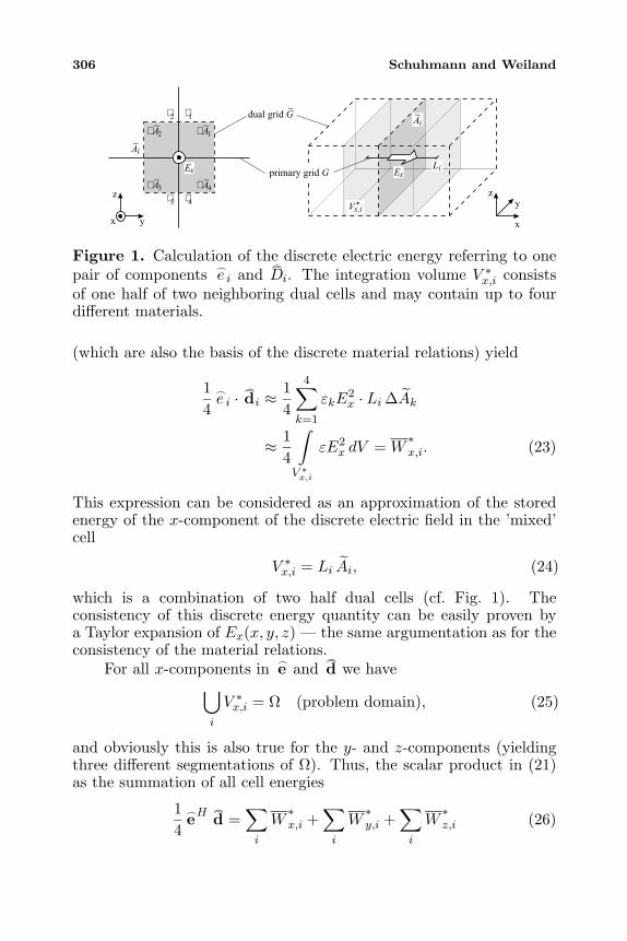
306 Schuhmann and Weiland
Li
Ai~
Ai~
ExEx
x
y
yx
zz
dual grid G~ 2
3 4
1
primary grid G
A1~ A2
~
A3~ A4
~
Vx,i*
Figure 1. Calculation of the discrete electric energy referring to onepair of components
e i andDi. The integration volume V ∗x,i consists
of one half of two neighboring dual cells and may contain up to fourdifferent materials.
(which are also the basis of the discrete material relations) yield
14e i ·
di ≈
14
4∑k=1
εkE2x · Li ∆Ak
≈ 14
∫V ∗x,i
εE2x dV = W
∗x,i. (23)
This expression can be considered as an approximation of the storedenergy of the x-component of the discrete electric field in the ’mixed’cell
V ∗x,i = Li Ai, (24)
which is a combination of two half dual cells (cf. Fig. 1). Theconsistency of this discrete energy quantity can be easily proven bya Taylor expansion of Ex(x, y, z) — the same argumentation as for theconsistency of the material relations.
For all x-components in e andd we have⋃
i
V ∗x,i = Ω (problem domain), (25)
and obviously this is also true for the y- and z-components (yieldingthree different segmentations of Ω). Thus, the scalar product in (21)as the summation of all cell energies
14eH
d =
∑i
W∗x,i +
∑i
W∗y,i +
∑i
W∗z,i (26)
Conservation laws in the finite integration technique 307
is the total stored discrete electric energy in the grid. The derivationof the magnetic energy is completely analogous.
For static or transient fields, where no time-averaging has to beperformed, the corresponding definitions are
We =12eT
d, Wm =
12
hTb. (27)
3. ENERGY CONSERVATION IN THE DISCRETESYSTEM
Based on this definition of the discrete energy we will now consider itstransient characteristics for time-varying fields [2, 7].
In a first step the time derivatives in (3) are left untouched,and thus the conservation of discrete energy is only analyzed for thespatial discretization scheme itself. This is sufficient, for example, fortime-harmonic fields, if the time-dependence is implicitly (and withoutapproximations) introduced by a complex exponential expression. Forthe general case of transient fields, however, the time axis has to bediscretized too, and thus also the time integration scheme applied toMaxwell’s Grid Equations has to be taken into account.
Discrete space – continuous time
The total discrete energy in the computational grid according to (27)is given by
W (t) = We(t) + Wm(t) =12(eT (t)
d(t) +
hT (t)b(t)). (28)
Exploiting the symmetry of the material matrices, we obtain for thetime derivative of this equation:
d
dtW (t) =
12
(d
dteT
d + eT
d
dt
d +
d
dt
hTb +
hTd
dt
b
)
=12
((Mε
e)Td
dte + eT
d
dt
d + (Mµ
h)Td
dt
h +
hTd
dt
b
)
= eTd
dt
d +
hTd
dt
b. (29)
Putting in Maxwell’s Grid Equations (3) and the duality relation (6),a discrete form of Poynting’s law for the total energy in the grid canbe derived:
d
dtW = eT (C
h −j )−
hTCe = −eTj . (30)
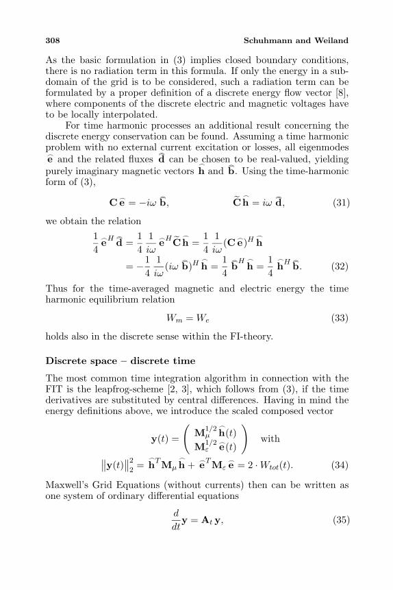
308 Schuhmann and Weiland
As the basic formulation in (3) implies closed boundary conditions,there is no radiation term in this formula. If only the energy in a sub-domain of the grid is to be considered, such a radiation term can beformulated by a proper definition of a discrete energy flow vector [8],where components of the discrete electric and magnetic voltages haveto be locally interpolated.
For time harmonic processes an additional result concerning thediscrete energy conservation can be found. Assuming a time harmonicproblem with no external current excitation or losses, all eigenmodese and the related fluxes
d can be chosen to be real-valued, yielding
purely imaginary magnetic vectors
h andb. Using the time-harmonic
form of (3),
Ce = −iω b, C
h = iωd, (31)
we obtain the relation14eH
d =
14
1iω
eHC
h =14
1iω
(Ce)H
h
= −14
1iω
(iωb)H
h =14
bH
h =14
hHb. (32)
Thus for the time-averaged magnetic and electric energy the timeharmonic equilibrium relation
Wm = We (33)
holds also in the discrete sense within the FI-theory.
Discrete space – discrete time
The most common time integration algorithm in connection with theFIT is the leapfrog-scheme [2, 3], which follows from (3), if the timederivatives are substituted by central differences. Having in mind theenergy definitions above, we introduce the scaled composed vector
y(t) =
(M1/2
µ
h(t)M1/2
εe(t)
)with
∥∥y(t)∥∥2
2=
hTMµ
h + eTMεe = 2 ·Wtot(t). (34)
Maxwell’s Grid Equations (without currents) then can be written asone system of ordinary differential equations
d
dty = At y, (35)
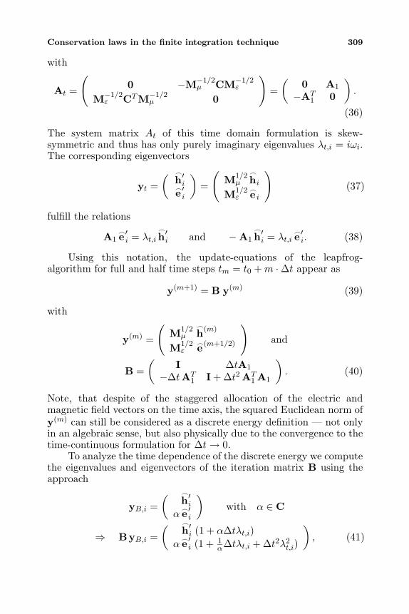
Conservation laws in the finite integration technique 309
with
At =
(0 −M−1/2
µ CM−1/2ε
M−1/2ε CTM−1/2
µ 0
)=
(0 A1
−AT1 0
).
(36)
The system matrix At of this time domain formulation is skew-symmetric and thus has only purely imaginary eigenvalues λt,i = iωi.The corresponding eigenvectors
yt =(
h′ie ′i
)=
(M1/2
µ
hiM1/2
εe i
)(37)
fulfill the relations
A1e ′i = λt,i
h′i and −A1
h′i = λt,ie ′i. (38)
Using this notation, the update-equations of the leapfrog-algorithm for full and half time steps tm = t0 + m ·∆t appear as
y(m+1) = B y(m) (39)
with
y(m) =
(M1/2
µ
h(m)
M1/2ε
e (m+1/2)
)and
B =(
I ∆tA1
−∆tAT1 I + ∆t2 AT
1 A1
). (40)
Note, that despite of the staggered allocation of the electric andmagnetic field vectors on the time axis, the squared Euclidean norm ofy(m) can still be considered as a discrete energy definition — not onlyin an algebraic sense, but also physically due to the convergence to thetime-continuous formulation for ∆t→ 0.
To analyze the time dependence of the discrete energy we computethe eigenvalues and eigenvectors of the iteration matrix B using theapproach
yB,i =(
h′iαe ′i
)with α ∈ C
⇒ ByB,i =(
h′i (1 + α∆tλt,i)αe ′i (1 + 1
α∆tλt,i + ∆t2λ2t,i)
), (41)
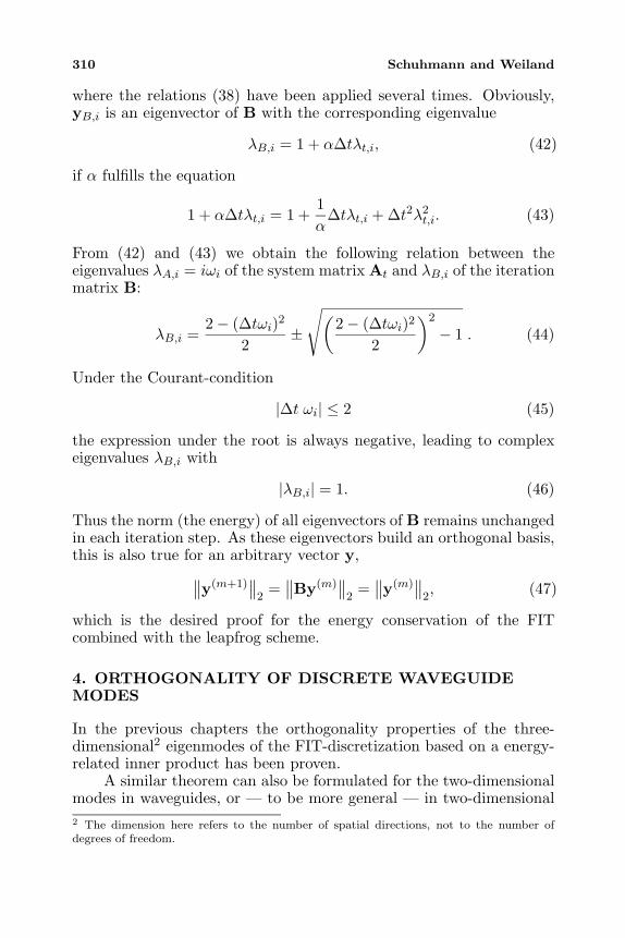
310 Schuhmann and Weiland
where the relations (38) have been applied several times. Obviously,yB,i is an eigenvector of B with the corresponding eigenvalue
λB,i = 1 + α∆tλt,i, (42)
if α fulfills the equation
1 + α∆tλt,i = 1 +1α
∆tλt,i + ∆t2λ2t,i. (43)
From (42) and (43) we obtain the following relation between theeigenvalues λA,i = iωi of the system matrix At and λB,i of the iterationmatrix B:
λB,i =2− (∆tωi)2
2±
√(2− (∆tωi)2
2
)2
− 1 . (44)
Under the Courant-condition
|∆t ωi| ≤ 2 (45)
the expression under the root is always negative, leading to complexeigenvalues λB,i with
|λB,i| = 1. (46)
Thus the norm (the energy) of all eigenvectors of B remains unchangedin each iteration step. As these eigenvectors build an orthogonal basis,this is also true for an arbitrary vector y,
∥∥y(m+1)∥∥
2=
∥∥By(m)∥∥
2=
∥∥y(m)∥∥
2, (47)
which is the desired proof for the energy conservation of the FITcombined with the leapfrog scheme.
4. ORTHOGONALITY OF DISCRETE WAVEGUIDEMODES
In the previous chapters the orthogonality properties of the three-dimensional2 eigenmodes of the FIT-discretization based on a energy-related inner product has been proven.
A similar theorem can also be formulated for the two-dimensionalmodes in waveguides, or — to be more general — in two-dimensional2 The dimension here refers to the number of spatial directions, not to the number ofdegrees of freedom.
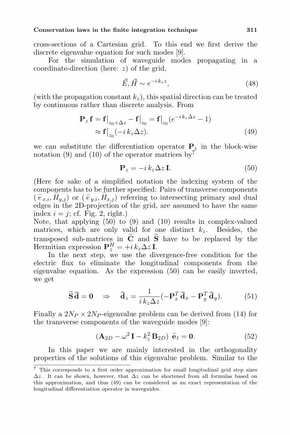
Conservation laws in the finite integration technique 311
cross-sections of a Cartesian grid. To this end we first derive thediscrete eigenvalue equation for such modes [9].
For the simulation of waveguide modes propagating in acoordinate-direction (here: z) of the grid,
E, H ∼ e−i kzz, (48)
(with the propagation constant kz), this spatial direction can be treatedby continuous rather than discrete analysis. From
Pz f = f∣∣z0+∆z
− f∣∣z0
= f∣∣z0
(e−i kz∆z − 1)
≈ f∣∣z0
(−i kz∆z). (49)
we can substitute the differentiation operator Pz in the block-wisenotation (9) and (10) of the operator matrices by7
Pz = −i kz∆z I. (50)
(Here for sake of a simplified notation the indexing system of thecomponents has to be further specified: Pairs of transverse components(e x,i,
Hy,j) or (e y,i,
Hx,j) referring to intersecting primary and dualedges in the 2D-projection of the grid, are assumed to have the sameindex i = j; cf. Fig. 2, right.)Note, that applying (50) to (9) and (10) results in complex-valuedmatrices, which are only valid for one distinct kz. Besides, thetransposed sub-matrices in C and S have to be replaced by theHermitian expression PH
z = +i kz∆z I.In the next step, we use the divergence-free condition for the
electric flux to eliminate the longitudinal components from theeigenvalue equation. As the expression (50) can be easily inverted,we get
Sd = 0 ⇒
dz =1
i kz∆z(−PT
x
dx −PT
y
dy). (51)
Finally a 2NP × 2NP -eigenvalue problem can be derived from (14) forthe transverse components of the waveguide modes [9]:
(A2D − ω2 I− k2z B2D) e t = 0. (52)
In this paper we are mainly interested in the orthogonalityproperties of the solutions of this eigenvalue problem. Similar to the7 This corresponds to a first order approximation for small longitudinal grid step sizes∆z. It can be shown, however, that ∆z can be shortened from all formulas based onthis approximation, and thus (49) can be considered as an exact representation of thelongitudinal differentiation operator in waveguides.
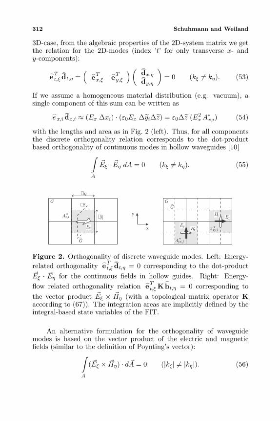
312 Schuhmann and Weiland
3D-case, from the algebraic properties of the 2D-system matrix we getthe relation for the 2D-modes (index ’t’ for only transverse x- andy-components):
eTt,ξdt,η =
(eTx,ξ
eTy,ξ) (
dx,ηdy,η
)= 0 (kξ = kη). (53)
If we assume a homogeneous material distribution (e.g. vacuum), asingle component of this sum can be written as
e x,i
dx,i ≈ (Ex ∆xi) · (ε0Ex ∆yi∆z) = ε0∆z (E2
xA∗x,i) (54)
with the lengths and area as in Fig. 2 (left). Thus, for all componentsthe discrete orthogonality relation corresponds to the dot-productbased orthogonality of continuous modes in hollow waveguides [10]∫
A
Eξ · Eη dA = 0 (kξ = kη). (55)
Ex
Ax,i*
x
y
G~
G~
G z~
ExHy
HxEy
G
y~i
xi
Axy,i*
Ayx,j*
Figure 2. Orthogonality of discrete waveguide modes. Left: Energy-related orthogonality eTt,ξ
dt,η = 0 corresponding to the dot-product
Eξ · Eη for the continuous fields in hollow guides. Right: Energy-flow related orthogonality relation eTt,ξ K
ht,η = 0 corresponding tothe vector product Eξ × Hη (with a topological matrix operator Kaccording to (67)). The integration areas are implicitly defined by theintegral-based state variables of the FIT.
An alternative formulation for the orthogonality of waveguidemodes is based on the vector product of the electric and magneticfields (similar to the definition of Poynting’s vector):∫
A
( Eξ × Hη) · d A = 0 (|kξ| = |kη|). (56)
Conservation laws in the finite integration technique 313
A corresponding theorem can be found for the discrete fields, too, andwe again only use Maxwell’s Grid Equations, the duality property (6),and the symmetry of the material matrices for its derivation. It isremarkable, that the algebraic proof is in close analogy to the classicalproof for continuous fields (cf. [10]).
We start with the discrete curl-equations in (3), applied to twowaveguide modes with kξ = ±kη. According to (50) two differentC-matrices (denoted Cξ and Cη) have to be used:
Cξeξ = −iω
bξ, Cηeη = −iω
bη. (57)
Left-multiplying by
hTη or
hTξ yields
hTηCξeξ = −iω
hTηbξ,
hTξ Cηeη = −iω
hTξbη, (58)
leading to (exploiting the symmetry of the magnetic material matrix)
hTηCξeξ −
hTξ Cηeη = −iω
((Mµ−1
bη)T
bξ − (Mµ−1
bξ)T
bη
)= −iω
(bTηM
Tµ−1
bξ −
bTξ M
Tµ−1
bη
)= 0. (59)
Analogously we obtain from the second curl-equation:
Cξ
hξ = iωdξ, Cη
hη = iωdη, (60)
eTη Cξ
hξ = iωeTη
dξ,
eTξ Cη
hη = iωeTξ
dη, (61)
eTη Cξ
hξ − eTξ Cη
hη = iω((M−1
ε
dη)T
dξ − (M−1
ε
dξ)T
dη
)= iω
(dTη (M−1
ε )Tdξ −
dTξ (M−1
ε )Tdη
)= 0.
(62)
Adding up (59) and (62) yields:
hTηCξeξ − eTξ Cη
hη −
hTξ Cηeη + eTη Cξ
hξ = 0
⇒ eTξ (CTξ − Cη)
hη − eTη (CTη − Cξ)
hξ = 0. (63)
If we introduce now the block-wise notation of C and C accordingto (9) and (50), we get
CTξ − Cη =
0 −ikξI −PT
v
ikξI 0 PTx
PTv −PT
x 0
−
0 ikηI −PT
v
−ikηI 0 PTx
PTv −PT
x 0
= −i(kξ + kη)
( 0 I 0−I 0 00 0 0
). (64)
314 Schuhmann and Weiland
Thus, the transverse fields
e t,ξ =(
ex,ξey,ξ
)
ht,ξ =(
hx,ξ
hy,ξ
)(65)
fulfill the relation
(kξ + kη)(eTt,ξ K
ht,η − eTt,η K
ht,ξ)
= 0, (66)
with the matrix operator
K =(
0 I−I 0
). (67)
For kξ = −kη as assumed above we finally geteTt,ξ K
ht,η − eTt,η K
ht,ξ = 0. (68)
If we change the sign of one of the propagation constants in thisderivation (for a wave propagation in the opposite direction),
k′ξ = −kξ, e ′t,ξ = e t,ξ,
h′t,ξ = −
ht,ξ. (69)
we get the relation
(−kξ + kη)(eTt,ξ K
ht,η + eTt,η K
ht,ξ)
= 0, (70)
instead of (66), leading to (for kξ = kη):eTt,ξ K
ht,η + eTt,η K
ht,ξ = 0. (71)
Adding up (68) and (71) finally yields the desired orthogonalityrelation for the discrete eigenmodes in waveguides:
eTt,ξ K
ht,η = 0 (kξ = ±kη). (72)
For each set of degenerated modes with kξ = ±kη a linear combinationcan be found such, that (72) is fulfilled, too.
The geometrical interpretation of this orthogonality relation isshown in Fig. 2 (right). By the entries ±1 in the topological operatorK, pairs of components
e x,i,
hy,i and e y,j ,
hx,j are coupled to eachother, which are related to perpendicular edges; and each product ofthe corresponding field strengths can be considered as a part of thedesired expression E× H. The grid sizes implied in the discrete voltagequantities define again integration areas A∗xy,i and A∗yx,j , which coverthe cross section of the waveguide. Thus, (72) can be identified as adiscrete analog of the integral over the vector product of Eξ and Hη in(56).
Conservation laws in the finite integration technique 315
5. CONCLUSION
In this paper we presented the concept of discrete energy quantitiesfor the electric and magnetic grid voltages — the state variables of theFinite Integration Technique — in a Cartesian grid system.
A central point of the derivation is the first-order interpretation ofthe discrete voltages as products of a continuous field quantity and themetric of the corresponding edges and facets of the grid. This leads tothe geometrical interpretation of the energy quantities as sum over allcell-energies, using different segmentations of the computation domain.
Several algebraic proofs for important properties of the FIT havebeen presented, including the energy conservation of the FIT bothin frequency and time domain, the energy-based orthogonality of thethree-dimensional eigenmodes, and two different formulations for theorthogonality of two-dimensional modes in longitudinally homogeneouswaveguides.
All these proofs are based on only a few algebraic properties ofthe discretization scheme — namely the duality of the discrete curl-operators and the definition of symmetric and positive definite materialmatrices. These properties thus can be considered to be key points ofthe formulation, and have to be preserved for any extensions of themethod (like e.g. sub-gridding techniques, non-orthogonal grids, orhigher-order schemes).
Not only the presented theorems themselves but also theirderivations and proofs within the discrete algebraic system are in closeanalogy to the vector-analytical analysis of continuous fields. TheFinite Integration Technique therefore can be considered as a uniqueand consistent discrete electromagnetic field theory.
REFERENCES
1. Weiland, T., “A discretization method for the solution ofMaxwell’s equations for six-component fields,” Electronics andCommunication (AEU), Vol. 31, 116–120, 1977.
2. Weiland, T., “Time domain electromagnetic field computationwith finite difference methods,” International Journal of Numer-ical Modelling: Electronic Networks, Devices and Fields, Vol. 9,259–319, 1996.
3. Yee, K. S., “Numerical solution of initial boundary value problemsinvolving Maxwell’s equations in isotropic media,” IEEE Trans.Ant. Prop., Vol. AP-14, 302–307, 1966.
4. van Rienen, U. and T. Weiland, “Triangular discretization method
316 Schuhmann and Weiland
for the evaluation of RF-fields in waveguides and cylindricallysymmetric cavities,” Particle Accelerators, Vol. 20, 239–267, 1987.
5. Schuhmann, R. and T. Weiland, “A stable interpolation techniquefor FDTD on nonorthogonal grids,” International Journal ofNumerical Modelling: Electronic Networks, Devices and Fields,Vol. 11, 299–306, 1998.
6. Clemens, M. and T. Weiland, “Discrete electromagnetism withthe finite integration technique,” this volume.
7. Thoma, P., “Numerical stability of finite difference time domainmethods,” IEEE Trans. Mag., Vol. 34, 2740–2743, 1998.
8. Thoma, P., “Zur numerischen Losung der MaxwellschenGleichungen im Zeitbereich,” Ph.D. Thesis, Darmstadt Universityof Technology, 1997.
9. Weiland, T., “A numerical method for the solution of theeigenwave problem of longitudinally homogeneous waveguides,”Electronics and Communication (AEU), Vol. 31, 308–314, 1977.
10. Collin, R. E., Field Theory of Guided Waves, McGraw-Hill, NewYork, 1960.
Progress In Electromagnetics Research, PIER 32, 317–356, 2001
COMPUTATIONAL ASPECTS OF THE CELL METHODIN ELECTRODYNAMICS
M. Marrone
DEEIUniversita di Trieste, Via Valerio 1034127 Trieste, Italy
Abstract—A desire to unify the mathematical description of manyphysical theories, such as electrodynamics, mechanics, thermalconduction, has led us to understand that global (=integral) physicalvariables of each theory can be associated to spatial geometricalelements such as points, lines, surfaces, volumes and temporalgeometrical elements such as instants and intervals. This associationhas led us to build a space-time classification diagram of variables andequations for each theory. Moreover, the possibility to express physicallaws directly in a finite rather than differential form has led to thedevelopment of a computational methodology called Cell Method [12].This paper discusses some practical aspects of this method and howit may overcome some of the main limitations of FDTD method inelectrodynamics. Moreover, we will provide some numerical examplesto compare the two methodologies.
1 Introduction
2 Theoretical Aspects of the Cell Method2.1 Space-Time Structure2.2 Orientation of Geometrical Elements2.3 Physical Global Variables of Electrodynamics2.4 Electrodynamic Laws2.5 Time Approximation2.6 Stability
3 The Delaunay-Voronoi Method3.1 Delaunay-Voronoi Grids
3.1.1 Two-Dimensional Extrude Grids
318 Marrone
3.1.2 Three-Dimensional Grids3.1.3 Orthogonality3.1.4 Cell Method and Delaunay-Voronoi Grids
3.2 Constitutive Equations3.2.1 Considerations on Maxwell-Ampere’s Law
3.3 Computational Algorithm3.4 Limits of the Delaunay-Voronoi Method
4 The Microcell Method4.1 Introduction4.2 Barycentric Grids
4.2.1 Two-Dimensional Extrude Case4.2.2 Three-Dimensional Case
4.3 Microcells4.4 Microcells and the Cell Method4.5 Constitutive Equations
4.5.1 Magnetic Constitutive Equation4.5.2 Electric Constitutive Equation4.5.3 Ohm’s Law
4.6 Considerations on Maxwell-Ampere’s Law4.7 Computational Algorithm4.8 Considerations on Microcell Method
5 Computational Aspects of the Cell Method5.1 Problem 1
5.1.1 Numerical Modeling of Problem 15.2 Problem 2
5.2.1 Numerical Modeling of Problem 25.3 Summary of Numerical Results
6 Conclusions
References
1. INTRODUCTION
Several numerical methods to find solutions to Maxwell’s equationshave been proposed over the years. One of them, possibly themost common and widespread, is the finite-difference time-domain(FDTD) method initially proposed by Yee [2] in 1966. Many studieshave been carried out on this method since then (see for example
Cell method in electrodynamics 319
[11]). In particular, many efforts have been directed to overcomingrestrictions in the FDTD method, such as the use of Cartesianorthogonal grids. The main techniques can be divided into two groupsarising, respectively, from the differential and the integral formulationof Maxwell’s equations:
• Differential formulation. One of the first methods using thisformulation is the FDTD method in generalized nonorthogonalcoordinates proposed by Holland [4] and then used, with somemodifications, by others [5, 6, 10].
• Integral formulation. In this context we can find many works:some of them are based on Delaunay-Voronoi grids [7, 9], otherson grids made by cells with more general shapes [8].
The general goal has been to arrive at a methodology which has thefollowing features [8]:
(i) Allows the use of unstructured non-orthogonal grids.(ii) Allows different types of cells (tetrahedral, cubic, etc.).(iii) Recovers the FDTD method when orthogonal grids are used.(iv) Preserves charge or divergence locally (and globally).(v) Conditionally stable.(vi) Non-dispersive.(vii) Non-dissipative.(viii) Accurate for non-orthogonal grids.
In this paper, we will describe a method, dubbed Cell Method, thatincorporates the features (i)–(v) and (viii) above (items (vi)–(vii) havenot been analyzed). The Cell Method is based on a formulationstrictly related to the integral formulation of Maxwell’s equations; ituses global variables of the electrodynamic fields (fluxes Φ,Ψ, voltagesV ,F , currents I, charge Qc) rather than differential ones (field vectorsB, D, E, H, current density J, charge density ρ). Moreover, wewill illustrate some results obtained using Cell Method, and includea comparison against results from the FDTD method and from a fullmodal expansion.
2. THEORETICAL ASPECTS OF THE CELL METHOD
2.1. Space-Time Structure
The cell method is based, as the first step, on a space-time structurethat consists of two spatial geometrical structures:
• Primal spatial grid G, defined by the set of primal elementsG = P,L, S, V that are points P, lines L, surfaces S, volumes V.
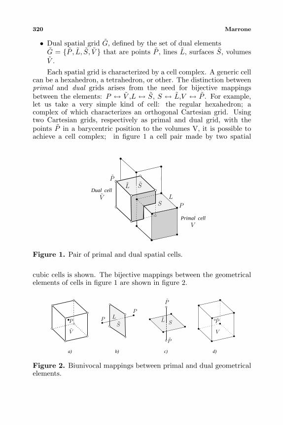
320 Marrone
• Dual spatial grid G, defined by the set of dual elementsG = P , L, S, V that are points P , lines L, surfaces S, volumesV .
Each spatial grid is characterized by a cell complex. A generic cellcan be a hexahedron, a tetrahedron, or other. The distinction betweenprimal and dual grids arises from the need for bijective mappingsbetween the elements: P ↔ V ,L ↔ S, S ↔ L,V ↔ P . For example,let us take a very simple kind of cell: the regular hexahedron; acomplex of which characterizes an orthogonal Cartesian grid. Usingtwo Cartesian grids, respectively as primal and dual grid, with thepoints P in a barycentric position to the volumes V, it is possible toachieve a cell complex; in figure 1 a cell pair made by two spatial
P
L
PL
V
S
S
VPrimal cell
Dual cell
Figure 1. Pair of primal and dual spatial cells.
cubic cells is shown. The bijective mappings between the geometricalelements of cells in figure 1 are shown in figure 2.
V
P
P
P
SLP
P
S
LP
V
a) b) c) d)
Figure 2. Biunivocal mappings between primal and dual geometricalelements.
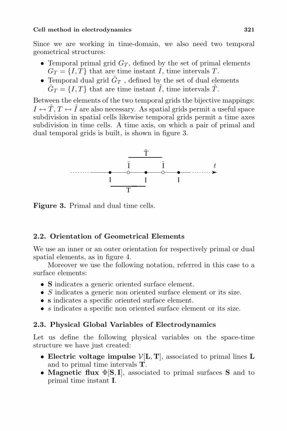
Cell method in electrodynamics 321
Since we are working in time-domain, we also need two temporalgeometrical structures:
• Temporal primal grid GT , defined by the set of primal elementsGT = I, T that are time instant I, time intervals T .• Temporal dual grid GT , defined by the set of dual elements
GT = I, T that are time instant I, time intervals T .
Between the elements of the two temporal grids the bijective mappings:I ↔ T , T ↔ I are also necessary. As spatial grids permit a useful spacesubdivision in spatial cells likewise temporal grids permit a time axessubdivision in time cells. A time axis, on which a pair of primal anddual temporal grids is built, is shown in figure 3.
t
˜
I I
T
I I I
T
Figure 3. Primal and dual time cells.
2.2. Orientation of Geometrical Elements
We use an inner or an outer orientation for respectively primal or dualspatial elements, as in figure 4.
Moreover we use the following notation, referred in this case to asurface elements:
• S indicates a generic oriented surface element.• S indicates a generic non oriented surface element or its size.• s indicates a specific oriented surface element.• s indicates a specific non oriented surface element or its size.
2.3. Physical Global Variables of Electrodynamics
Let us define the following physical variables on the space-timestructure we have just created:
• Electric voltage impulse V[L,T], associated to primal lines Land to primal time intervals T.
• Magnetic flux Φ[S, I], associated to primal surfaces S and toprimal time instant I.
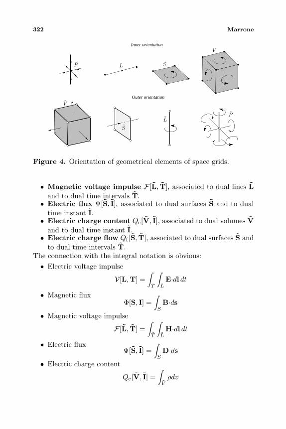
322 Marrone
V
S
Inner orientation
Outer orientation
PL
V
L
S
P
Figure 4. Orientation of geometrical elements of space grids.
• Magnetic voltage impulse F [L, T], associated to dual lines Land to dual time intervals T.
• Electric flux Ψ[S, I], associated to dual surfaces S and to dualtime instant I.• Electric charge content Qc[V, I], associated to dual volumes V
and to dual time instant I.• Electric charge flow Qf [S, T], associated to dual surfaces S and
to dual time intervals T.The connection with the integral notation is obvious:• Electric voltage impulse
V[L,T] =∫T
∫LE·dl dt
• Magnetic fluxΦ[S, I] =
∫SB·ds
• Magnetic voltage impulse
F [L, T] =∫T
∫LH·dl dt
• Electric fluxΨ[S, I] =
∫SD·ds
• Electric charge content
Qc[V, I] =∫Vρdv
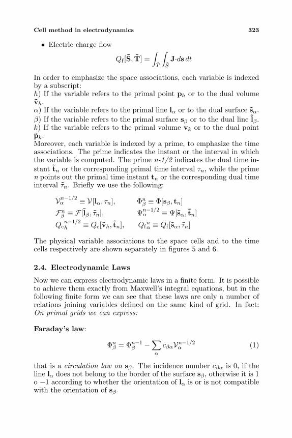
Cell method in electrodynamics 323
• Electric charge flow
Qf [S, T] =∫T
∫SJ·ds dt
In order to emphasize the space associations, each variable is indexedby a subscript:h) If the variable refers to the primal point ph or to the dual volumevh.α) If the variable refers to the primal line lα or to the dual surface sα.β) If the variable refers to the primal surface sβ or to the dual line lβ.k) If the variable refers to the primal volume vk or to the dual pointpk.Moreover, each variable is indexed by a prime, to emphasize the timeassociations. The prime indicates the instant or the interval in whichthe variable is computed. The prime n-1/2 indicates the dual time in-stant tn or the corresponding primal time interval τn, while the primen points out the primal time instant tn or the corresponding dual timeinterval τn. Briefly we use the following:
Vn−1/2α ≡ V[lα, τn], Φn
β ≡ Φ[sβ, tn]
Fnβ ≡ F [lβ, τn], Ψn−1/2α ≡ Ψ[sα, tn]
Qcn−1/2h ≡ Qc[vh, tn], Qf
nα ≡ Qf [sα, τn]
The physical variable associations to the space cells and to the timecells respectively are shown separately in figures 5 and 6.
2.4. Electrodynamic Laws
Now we can express electrodynamic laws in a finite form. It is possibleto achieve them exactly from Maxwell’s integral equations, but in thefollowing finite form we can see that these laws are only a number ofrelations joining variables defined on the same kind of grid. In fact:On primal grids we can express:
Faraday’s law:
Φnβ = Φn−1
β −∑α
cβαVn−1/2α (1)
that is a circulation law on sβ. The incidence number cβα is 0, if theline lα does not belong to the border of the surface sβ, otherwise it is 1o −1 according to whether the orientation of lα is or is not compatiblewith the orientation of sβ.
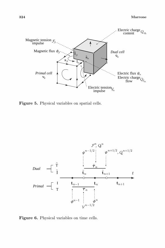
324 Marrone
Electric tensionimpulse
content
flow
impulseMagnetic tension
Magnetic flux Φ
Electric flux ΨElectric charge
Primal cell
Dual cell
l
ββ
s
l
α
αs hv
kv
Electric chargeh
Q c
α
β
αQ f
αV
βF
Figure 5. Physical variables on spatial cells.
τ n
tn
n
n
tn−1
n−1/2
n−1/2
n−1
t
t
,,
tn tn+1
n+1
n+1/2
n
n+1/2
τ n
I
˜
˜Dual
T
PrimalI
T
Φ Φ
ΨΨ
V
FQc
Qf
Figure 6. Physical variables on time cells.
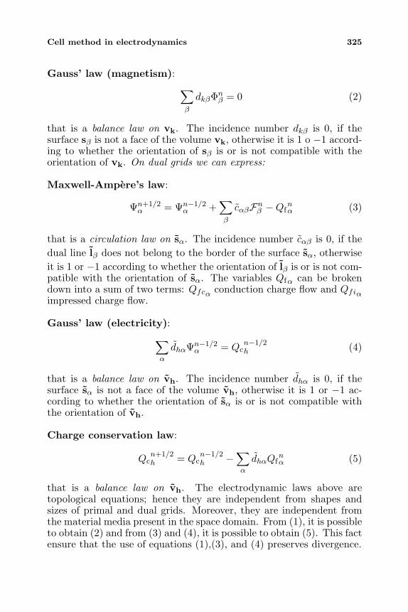
Cell method in electrodynamics 325
Gauss’ law (magnetism):∑β
dkβΦnβ = 0 (2)
that is a balance law on vk. The incidence number dkβ is 0, if thesurface sβ is not a face of the volume vk, otherwise it is 1 o −1 accord-ing to whether the orientation of sβ is or is not compatible with theorientation of vk. On dual grids we can express:
Maxwell-Ampere’s law:
Ψn+1/2α = Ψn−1/2
α +∑β
cαβFnβ −Qfnα (3)
that is a circulation law on sα. The incidence number cαβ is 0, if thedual line lβ does not belong to the border of the surface sα, otherwiseit is 1 or −1 according to whether the orientation of lβ is or is not com-patible with the orientation of sα. The variables Qfα can be brokendown into a sum of two terms: Qfcα conduction charge flow and Qfiαimpressed charge flow.
Gauss’ law (electricity):∑α
dhαΨn−1/2α = Qc
n−1/2h (4)
that is a balance law on vh. The incidence number dhα is 0, if thesurface sα is not a face of the volume vh, otherwise it is 1 or −1 ac-cording to whether the orientation of sα is or is not compatible withthe orientation of vh.
Charge conservation law:
Qcn+1/2h = Qc
n−1/2h −
∑α
dhαQfnα (5)
that is a balance law on vh. The electrodynamic laws above aretopological equations; hence they are independent from shapes andsizes of primal and dual grids. Moreover, they are independent fromthe material media present in the space domain. From (1), it is possibleto obtain (2) and from (3) and (4), it is possible to obtain (5). This factensure that the use of equations (1),(3), and (4) preserves divergence.
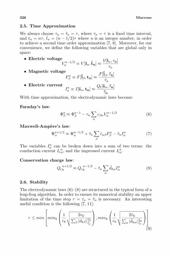
326 Marrone
2.5. Time Approximation
We always choose τn = τn = τ , where τn = τ is a fixed time interval,and tn = nτ , tn = (n − 1/2)τ where n is an integer number, in orderto achieve a second time order approximation [7, 8]. Moreover, for ourconvenience, we define the following variables that are global only inspace:• Electric voltage
V n−1/2α ≡ V [lα, tn] ≈ V[lα, τn]
τn• Magnetic voltage
Fnβ ≡ F [lβ, tn] ≈ F [lβ, τn]
τn• Electric current
Inα ≡ I [sα, tn] ≈ Qf [sα, τn]τn
With time approximation, the electrodynamic laws become:
Faraday’s law:
Φnβ ≈ Φn−1
β − τn∑α
cβαVn−1/2α (6)
Maxwell-Ampere’s law:
Ψn+1/2α ≈ Ψn−1/2
α + τn∑β
cαβFnβ − τnI
nα (7)
The variables Inα can be broken down into a sum of two terms: theconduction current Ic
nα, and the impressed current Ii
nα.
Conservation charge law:
Qcn+1/2h ≈ Qc
n−1/2h − τn
∑α
dhαInα (8)
2.6. Stability
The electrodynamic laws (6)–(8) are structured in the typical form of aleap-frog algorithm. In order to ensure its numerical stability an upperlimitation of the time step τ = τn = τn is necessary. An interestinguseful condition is the following [7, 11]:
τ ≤ min
mink
1
ck
√√√√ 2vk∑β |dkβ |
sβlβ
,minh
1
ch
√√√√ 2vh∑α |dhα| sαlα
(9)
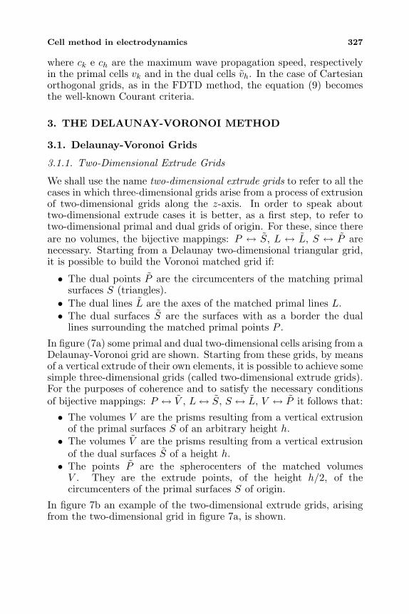
Cell method in electrodynamics 327
where ck e ch are the maximum wave propagation speed, respectivelyin the primal cells vk and in the dual cells vh. In the case of Cartesianorthogonal grids, as in the FDTD method, the equation (9) becomesthe well-known Courant criteria.
3. THE DELAUNAY-VORONOI METHOD
3.1. Delaunay-Voronoi Grids
3.1.1. Two-Dimensional Extrude Grids
We shall use the name two-dimensional extrude grids to refer to all thecases in which three-dimensional grids arise from a process of extrusionof two-dimensional grids along the z-axis. In order to speak abouttwo-dimensional extrude cases it is better, as a first step, to refer totwo-dimensional primal and dual grids of origin. For these, since thereare no volumes, the bijective mappings: P ↔ S, L ↔ L, S ↔ P arenecessary. Starting from a Delaunay two-dimensional triangular grid,it is possible to build the Voronoi matched grid if:
• The dual points P are the circumcenters of the matching primalsurfaces S (triangles).
• The dual lines L are the axes of the matched primal lines L.• The dual surfaces S are the surfaces with as a border the dual
lines surrounding the matched primal points P .
In figure (7a) some primal and dual two-dimensional cells arising from aDelaunay-Voronoi grid are shown. Starting from these grids, by meansof a vertical extrude of their own elements, it is possible to achieve somesimple three-dimensional grids (called two-dimensional extrude grids).For the purposes of coherence and to satisfy the necessary conditionsof bijective mappings: P ↔ V , L↔ S, S ↔ L, V ↔ P it follows that:
• The volumes V are the prisms resulting from a vertical extrusionof the primal surfaces S of an arbitrary height h.• The volumes V are the prisms resulting from a vertical extrusion
of the dual surfaces S of a height h.• The points P are the spherocenters of the matched volumes
V . They are the extrude points, of the height h/2, of thecircumcenters of the primal surfaces S of origin.
In figure 7b an example of the two-dimensional extrude grids, arisingfrom the two-dimensional grid in figure 7a, is shown.
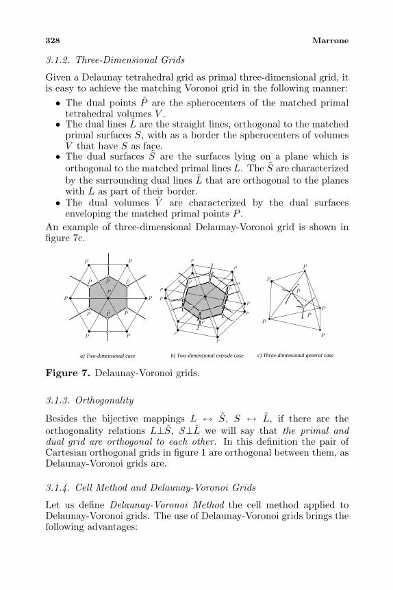
328 Marrone
3.1.2. Three-Dimensional Grids
Given a Delaunay tetrahedral grid as primal three-dimensional grid, itis easy to achieve the matching Voronoi grid in the following manner:• The dual points P are the spherocenters of the matched primal
tetrahedral volumes V .• The dual lines L are the straight lines, orthogonal to the matched
primal surfaces S, with as a border the spherocenters of volumesV that have S as face.
• The dual surfaces S are the surfaces lying on a plane which isorthogonal to the matched primal lines L. The S are characterizedby the surrounding dual lines L that are orthogonal to the planeswith L as part of their border.• The dual volumes V are characterized by the dual surfaces
enveloping the matched primal points P .An example of three-dimensional Delaunay-Voronoi grid is shown infigure 7c.
a) Two-dimensional case b) Two-dimensional extrude case c) Three-dimensional general case
P
P
P
P
P
P P
P
PP
PP
P
P
P
P
P
P P
P P
P
P
P
P
P
P
P
P
P
P
Figure 7. Delaunay-Voronoi grids.
3.1.3. Orthogonality
Besides the bijective mappings L ↔ S, S ↔ L, if there are theorthogonality relations L⊥S, S⊥L we will say that the primal anddual grid are orthogonal to each other. In this definition the pair ofCartesian orthogonal grids in figure 1 are orthogonal between them, asDelaunay-Voronoi grids are.
3.1.4. Cell Method and Delaunay-Voronoi Grids
Let us define Delaunay-Voronoi Method the cell method applied toDelaunay-Voronoi grids. The use of Delaunay-Voronoi grids brings thefollowing advantages:
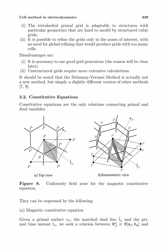
Cell method in electrodynamics 329
(i) The tetrahedral primal grid is adaptable to structures withparticular geometries that are hard to model by structured cubicgrids.
(ii) It is possible to refine the grids only in the zones of interest, withno need for global refining that would produce grids with too manycells.
Disadvantages are:(i) It is necessary to use good grid generators (the reason will be clear
later).(ii) Unstructured grids require more extensive calculations.It should be noted that the Delaunay-Voronoi Method is actually nota new method, but simply a slightly different version of other methods[7, 9].
3.2. Constitutive Equations
Constitutive equations are the only relations connecting primal anddual variables.
sβ
sβ
a) Top view b)Axonometric view
P
P
P
P
P P
PP
P
P
P
P P
P
P
P
P
P
PP
βlβl
Figure 8. Uniformity field zone for the magnetic constitutiveequation.
They can be expressed by the following:
(a) Magnetic constitutive equation
Given a primal surface sβ, the matched dual line lα and the pri-mal time instant tn, we seek a relation between Φn
β ≡ Φ[sβ, tn] and
330 Marrone
Fnβ ≡ F [lβ](tn). If there is a uniform magnetic field and a uniform
permeability µ in a zone containing sβ and lβ, as in figure 8 for a two-dimensional extrude case and, since sβ⊥lβ, the magnetic constitutiveequation may be expressed as:
Φ[sβ, tn]sβ
= µF [lβ](tn)
lβor
Φnβ
sβ= µ
Fnβ
lβ(10)
(b) Electric constitutive equation
Given a dual surface sα, the matched primal line lβ and the dualtime instant tn, we seek a relation between Ψn−1/2
α ≡ Ψ[sα, tn] andVn−1/2α ≡ V [lα](tn). If there is a uniform electric field and a uniform
dielectric constant ε in a zone containing sα and lα, since sα⊥lα theelectric constitutive equation may be expressed as:
Ψ[sα, tn]sα
= εV [lα](tn)
lαor
Ψn+1/2α
sα= ε
Vn+1/2α
lα(11)
(c) Ohm’s law:
Given a dual surface sα, the matched primal line lβ and the dualtime instant tn, we seek a relation between Inα ≡ I [sα](tn) andV nα ≡ V [lα](tn). If there is a uniform electric field and a uniform
conductivity constant σ in a zone containing sα and lα, since sα⊥lαOhm’s law may be expressed as:
I [sα](tn)sα
= σV [lα](tn)
lαor
Inαsα
= σV nα
lα(12)
Let us note that the variable V nα ≡ V [lα](tn), in Ohm’s law, does not
exist on the structures just created, because it is matched to the dualtime instant tn. Hence it must be estimated by means of some timeapproximations:
• Explicit approximation
V n ∼= aV n−1/2 + bV n−3/2 + ... (13)
with a,b,... numerical coefficients. This approximation needs otherlimitations on the value τ (as τ < ε
σ ), besides the limit (9), toensure the stability of the leap-frog algorithm.
Cell method in electrodynamics 331
• Implicit approximation
V n ∼= ... + aV n+1/2 + bV n−1/2 + ... (14)
with a,b,... numerical coefficients. This approximation does notrequire the limitations of explicit approximation. The assumption
V n ∼= V n+1/2 + V n−1/2
2(15)
used in the FDTD method [11], is an example of semi-implicitapproximation. The Ohm’s law with semi-implicit approximationbecomes
Inαsα
= σVn+1/2α + V
n−1/2α
2 lα(16)
3.2.1. Considerations on Maxwell-Ampere’s Law
Using the electric constitutive equation (11) and the Ohm’s law (16),the Maxwell-Ampere’s law becomes
Ψn+1/2α = Ψn−1/2
α + τn∑β
cαβFnβ − τnIi
nα − τn
σ
2ε(Ψn+1/2
α + Ψn−1/2α )
(17)This implicit approximation can be explicitly expressed as
Ψn+1/2α =
(1− τnσ
2ε
1 + τnσ2ε
)Ψn−1/2α +
(τn
1 + τnσ2ε
)(∑β
cαβFnβ − Ii
nα) (18)
3.3. Computational Algorithm
Starting from the initial conditionsI−1α = 0, V −1/2
α = 0⇒ Ψ−1/2α = 0, F 0
β = 0⇒ Φ0β = 0
the variables of the electrodynamic field, generated by an impressedcurrent starting from the initial time instant n = 0, can be computedthrough the following steps:
• Computation of Ψ1/2α by the Maxwell-Ampere’s law (18).
• Computation of V1/2α by the electric constitutive equations (11)
and by any boundary conditions.• Computation of Φ1
β by the Faraday’s law (6).
• Computation of F 1β by the magnetic constitutive equation (10)
and by any boundary conditions.• Iterate
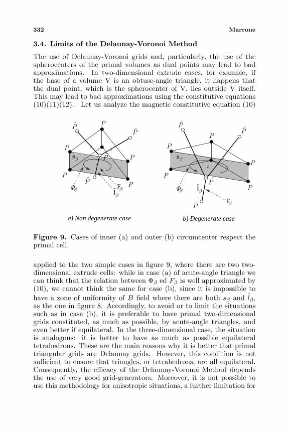
332 Marrone
3.4. Limits of the Delaunay-Voronoi Method
The use of Delaunay-Voronoi grids and, particularly, the use of thespherocenters of the primal volumes as dual points may lead to badapproximations. In two-dimensional extrude cases, for example, ifthe base of a volume V is an obtuse-angle triangle, it happens thatthe dual point, which is the spherocenter of V, lies outside V itself.This may lead to bad approximations using the constitutive equations(10)(11)(12). Let us analyze the magnetic constitutive equation (10)
a) Non degenerate case b) Degenerate case
P
P
P
P
P
P
P
P
P
P
P
PP
P
P
PP
P
βlβl
sβ sβ
Fβ
Fβ ΦβΦβ
Figure 9. Cases of inner (a) and outer (b) circumcenter respect theprimal cell.
applied to the two simple cases in figure 9, where there are two two-dimensional extrude cells: while in case (a) of acute-angle triangle wecan think that the relation between Φβ ed Fβ is well approximated by(10), we cannot think the same for case (b), since it is impossible tohave a zone of uniformity of B field where there are both sβ and lβ,as the one in figure 8. Accordingly, to avoid or to limit the situationssuch as in case (b), it is preferable to have primal two-dimensionalgrids constituted, as much as possible, by acute-angle triangles, andeven better if equilateral. In the three-dimensional case, the situationis analogous: it is better to have as much as possible equilateraltetrahedrons. These are the main reasons why it is better that primaltriangular grids are Delaunay grids. However, this condition is notsufficient to ensure that triangles, or tetrahedrons, are all equilateral.Consequently, the efficacy of the Delaunay-Voronoi Method dependsthe use of very good grid-generators. Moreover, it is not possible touse this methodology for anisotropic situations, a further limitation for
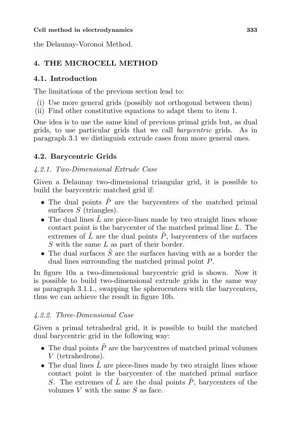
Cell method in electrodynamics 333
the Delaunay-Voronoi Method.
4. THE MICROCELL METHOD
4.1. Introduction
The limitations of the previous section lead to:
(i) Use more general grids (possibly not orthogonal between them)(ii) Find other constitutive equations to adapt them to item 1.
One idea is to use the same kind of previous primal grids but, as dualgrids, to use particular grids that we call barycentric grids. As inparagraph 3.1 we distinguish extrude cases from more general ones.
4.2. Barycentric Grids
4.2.1. Two-Dimensional Extrude Case
Given a Delaunay two-dimensional triangular grid, it is possible tobuild the barycentric matched grid if:
• The dual points P are the barycenters of the matched primalsurfaces S (triangles).• The dual lines L are piece-lines made by two straight lines whose
contact point is the barycenter of the matched primal line L. Theextremes of L are the dual points P , barycenters of the surfacesS with the same L as part of their border.
• The dual surfaces S are the surfaces having with as a border thedual lines surrounding the matched primal point P .
In figure 10a a two-dimensional barycentric grid is shown. Now itis possible to build two-dimensional extrude grids in the same wayas paragraph 3.1.1., swapping the spherocenters with the barycenters,thus we can achieve the result in figure 10b.
4.2.2. Three-Dimensional Case
Given a primal tetrahedral grid, it is possible to build the matcheddual barycentric grid in the following way:
• The dual points P are the barycentres of matched primal volumesV (tetrahedrons).
• The dual lines L are piece-lines made by two straight lines whosecontact point is the barycenter of the matched primal surfaceS. The extremes of L are the dual points P , barycenters of thevolumes V with the same S as face.
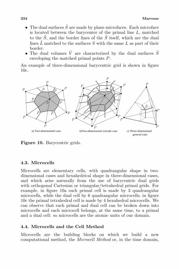
334 Marrone
• The dual surfaces S are made by plane microfaces. Each microfaceis located between the barycenter of the primal line L, matchedto the S, and the border lines of the S itself, which are the duallines L matched to the surfaces S with the same L as part of theirborder.
• The dual volumes V are characterized by the dual surfaces Senveloping the matched primal points P .
An example of three-dimensional barycentric grid is shown in figure10c.
P
P
PP
P
P
PP
P
P
P
P
P
P
P
P
P
P P
PP
PP
P
a) Two-dimensional case c) Three-dimensional general case
b)Two-dimensional extrude case
Figure 10. Barycentric grids.
4.3. Microcells
Microcells are elementary cells, with quadrangular shape in two-dimensional cases and hexahedrical shape in three-dimensional cases,and which arise naturally from the use of barycentric dual gridswith orthogonal Cartesian or triangular/tetrahedral primal grids. Forexample, in figure 10a each primal cell is made by 3 quadrangularmicrocells, while the dual cell by 6 quadrangular microcells; in figure10c the primal tetrahedral cell is made by 4 hexahedral microcells. Wecan observe that each primal and dual cell can be broken down intomicrocells and each microcell belongs, at the same time, to a primaland a dual cell: so microcells are the atomic units of our domain.
4.4. Microcells and the Cell Method
Microcells are the building blocks on which we build a newcomputational method, the Microcell Method or, in the time domain,
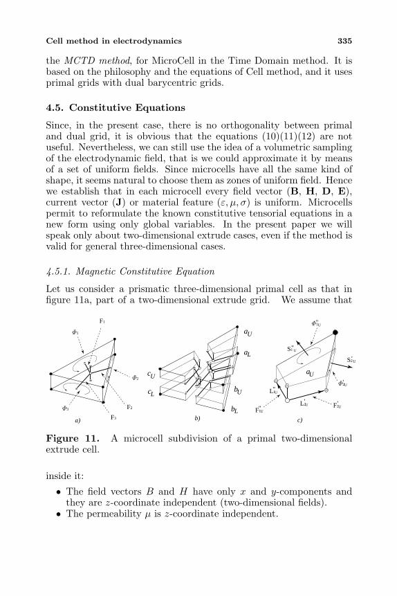
Cell method in electrodynamics 335
the MCTD method, for MicroCell in the Time Domain method. It isbased on the philosophy and the equations of Cell method, and it usesprimal grids with dual barycentric grids.
4.5. Constitutive Equations
Since, in the present case, there is no orthogonality between primaland dual grid, it is obvious that the equations (10)(11)(12) are notuseful. Nevertheless, we can still use the idea of a volumetric samplingof the electrodynamic field, that is we could approximate it by meansof a set of uniform fields. Since microcells have all the same kind ofshape, it seems natural to choose them as zones of uniform field. Hencewe establish that in each microcell every field vector (B, H, D, E),current vector (J) or material feature (ε, µ, σ) is uniform. Microcellspermit to reformulate the known constitutive tensorial equations in anew form using only global variables. In the present paper we willspeak only about two-dimensional extrude cases, even if the method isvalid for general three-dimensional cases.
4.5.1. Magnetic Constitutive Equation
Let us consider a prismatic three-dimensional primal cell as that infigure 11a, part of a two-dimensional extrude grid. We assume that
Φ2
Φ3
Φ1
F2
F3
F1
a)
Φ1
Φ2
F2
'
'F1"U
L1"U
UL2'U
U
S2'U
U"
S1 U"
cU
L
L
L
U
U
U
a
a
bc
b
a
b) c)
Figure 11. A microcell subdivision of a primal two-dimensionalextrude cell.
inside it:
• The field vectors B and H have only x and y-components andthey are z-coordinate independent (two-dimensional fields).
• The permeability µ is z-coordinate independent.
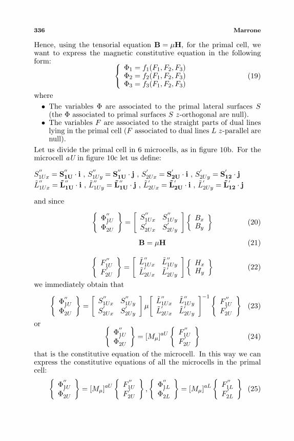
336 Marrone
Hence, using the tensorial equation B = µH, for the primal cell, wewant to express the magnetic constitutive equation in the followingform:
Φ1 = f1(F1, F2, F3)Φ2 = f2(F1, F2, F3)Φ3 = f3(F1, F2, F3)
(19)
where• The variables Φ are associated to the primal lateral surfaces S
(the Φ associated to primal surfaces S z-orthogonal are null).• The variables F are associated to the straight parts of dual lines
lying in the primal cell (F associated to dual lines L z-parallel arenull).
Let us divide the primal cell in 6 microcells, as in figure 10b. For themicrocell aU in figure 10c let us define:
S′′1Ux = S
′′1U · i , S
′′1Uy = S
′′1U · j , S
′2Ux = S
′2U · i , S
′2Uy = S
′12 · j
L′′1Ux = L
′′1U · i , L
′′1Uy = L
′′1U · j , L
′2Ux = L
′2U · i , L
′2Uy = L
′12 · j
and since
Φ′′1U
Φ′2U
=
[S′′1Ux S
′′1Uy
S′2Ux S
′2Uy
] Bx
By
(20)
B = µH (21)
F′′1U
F′2U
=
[L′′1Ux L
′′1Uy
L′2Ux L
′2Uy
] Hx
Hy
(22)
we immediately obtain that
Φ′′1U
Φ′2U
=
[S′′1Ux S
′′1Uy
S′2Ux S
′2Uy
]µ
[L′′1Ux L
′′1Uy
L′2Ux L
′2Uy
]−1 F′′1U
F′2U
(23)
or Φ′′1U
Φ′2U
= [Mµ]
aU
F′′1U
F′2U
(24)
that is the constitutive equation of the microcell. In this way we canexpress the constitutive equations of all the microcells in the primalcell:
Φ′′1U
Φ′2U
= [Mµ]
aU
F′′1U
F′2U
,
Φ′′1L
Φ′2L
= [Mµ]
aL
F′′1L
F′2L
(25)
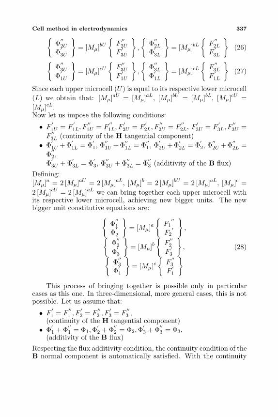
Cell method in electrodynamics 337
Φ′′2U
Φ′3U
= [Mµ]
bU
F′′2U
F′3U
,
Φ′′2L
Φ′3L
= [Mµ]
bL
F′′2L
F′3L
(26)
Φ′′3U
Φ′1U
= [Mµ]
cU
F′′3U
F′1U
,
Φ′′3L
Φ′1L
= [Mµ]
cL
F′′3L
F′1L
(27)
Since each upper microcell (U) is equal to its respective lower microcell(L) we obtain that: [Mµ]
aU = [Mµ]aL, [Mµ]
bU = [Mµ]bL, [Mµ]
cU =[Mµ]
cL.Now let us impose the following conditions:
• F′1U = F
′1L, F
′′1U = F
′′1L, F
′2U = F
′2L, F
′′2U = F
′′2L, F
′3U = F
′3L, F
′′3U =
F′′3L (continuity of the H tangential component)
• Φ′1U +Φ
′1L = Φ
′1, Φ
′′1U +Φ
′′1L = Φ
′′1 , Φ
′2U +Φ
′2L = Φ
′2, Φ
′′2U +Φ
′′2L =
Φ′′2 ,
Φ′3U + Φ
′3L = Φ
′3, Φ
′′3U + Φ
′′3L = Φ
′′3 (additivity of the B flux)
Defining:[Mµ]
a = 2 [Mµ]aU = 2 [Mµ]
aL, [Mµ]b = 2 [Mµ]
bU = 2 [Mµ]aL, [Mµ]
c =2 [Mµ]
cU = 2 [Mµ]aL we can bring together each upper microcell with
its respective lower microcell, achieving new bigger units. The newbigger unit constitutive equations are:
Φ′′1
Φ′2
= [Mµ]
a
F1′′
F2′
,
Φ′′2
Φ′3
= [Mµ]
b
F′′2
F′3
,
Φ′′3
Φ′1
= [Mµ]
c
F′′3
F′1
(28)
This process of bringing together is possible only in particularcases as this one. In three-dimensional, more general cases, this is notpossible. Let us assume that:
• F′1 = F
′′1 , F
′2 = F
′′2 , F
′3 = F
′′3 ,
(continuity of the H tangential component)• Φ
′1 + Φ
′′1 = Φ1,Φ
′2 + Φ
′′2 = Φ2,Φ
′3 + Φ
′′3 = Φ3,
(additivity of the B flux)
Respecting the flux additivity condition, the continuity condition of theB normal component is automatically satisfied. With the continuity
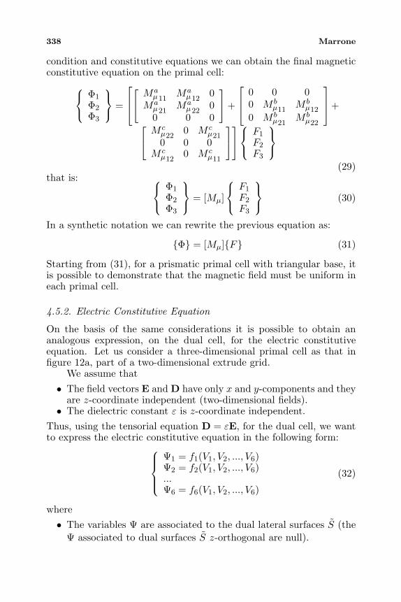
338 Marrone
condition and constitutive equations we can obtain the final magneticconstitutive equation on the primal cell:
Φ1
Φ2
Φ3
=
Ma
µ11Ma
µ120
Maµ21
Maµ22
00 0 0
+
0 0 00 M b
µ11M b
µ120 M b
µ21M b
µ22
+
M c
µ220 M c
µ210 0 0
M cµ12
0 M cµ11
F1
F2
F3
(29)that is:
Φ1
Φ2
Φ3
= [Mµ]
F1
F2
F3
(30)
In a synthetic notation we can rewrite the previous equation as:
Φ = [Mµ]F (31)
Starting from (31), for a prismatic primal cell with triangular base, itis possible to demonstrate that the magnetic field must be uniform ineach primal cell.
4.5.2. Electric Constitutive Equation
On the basis of the same considerations it is possible to obtain ananalogous expression, on the dual cell, for the electric constitutiveequation. Let us consider a three-dimensional primal cell as that infigure 12a, part of a two-dimensional extrude grid.
We assume that• The field vectors E and D have only x and y-components and they
are z-coordinate independent (two-dimensional fields).• The dielectric constant ε is z-coordinate independent.
Thus, using the tensorial equation D = εE, for the dual cell, we wantto express the electric constitutive equation in the following form:
Ψ1 = f1(V1, V2, ..., V6)Ψ2 = f2(V1, V2, ..., V6)...Ψ6 = f6(V1, V2, ..., V6)
(32)
where• The variables Ψ are associated to the dual lateral surfaces S (the
Ψ associated to dual surfaces S z-orthogonal are null).
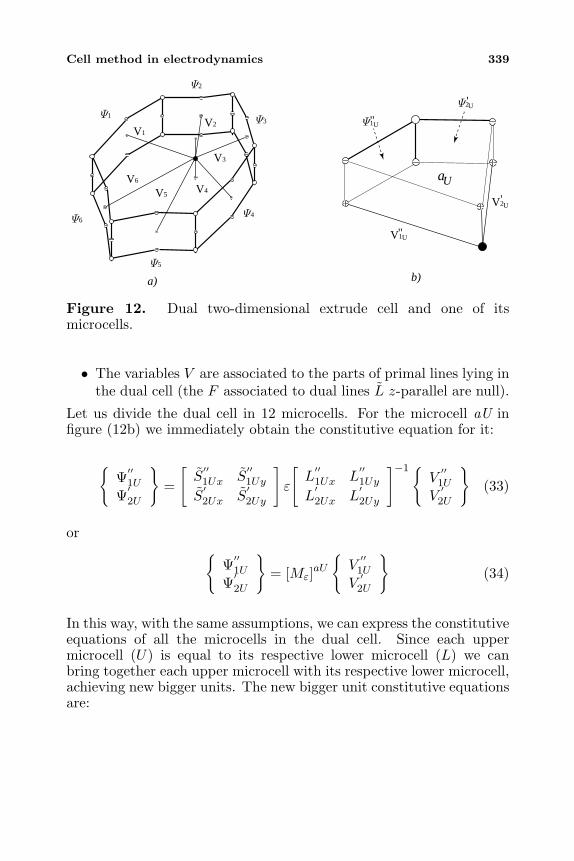
Cell method in electrodynamics 339
a)
Ψ2
Ψ1Ψ1
Ψ2
Ψ3
Ψ4
Ψ5
Ψ6
V2
V1
V1V2
V3
V4V5
V6
b)
U
U
U
U
"
"
'
'
Ua
Figure 12. Dual two-dimensional extrude cell and one of itsmicrocells.
• The variables V are associated to the parts of primal lines lying inthe dual cell (the F associated to dual lines L z-parallel are null).
Let us divide the dual cell in 12 microcells. For the microcell aU infigure (12b) we immediately obtain the constitutive equation for it:
Ψ′′1U
Ψ′2U
=
[S′′1Ux S
′′1Uy
S′2Ux S
′2Uy
]ε
[L′′1Ux L
′′1Uy
L′2Ux L
′2Uy
]−1 V′′1U
V′2U
(33)
or
Ψ′′1U
Ψ′2U
= [Mε]
aU
V′′1U
V′2U
(34)
In this way, with the same assumptions, we can express the constitutiveequations of all the microcells in the dual cell. Since each uppermicrocell (U) is equal to its respective lower microcell (L) we canbring together each upper microcell with its respective lower microcell,achieving new bigger units. The new bigger unit constitutive equationsare:
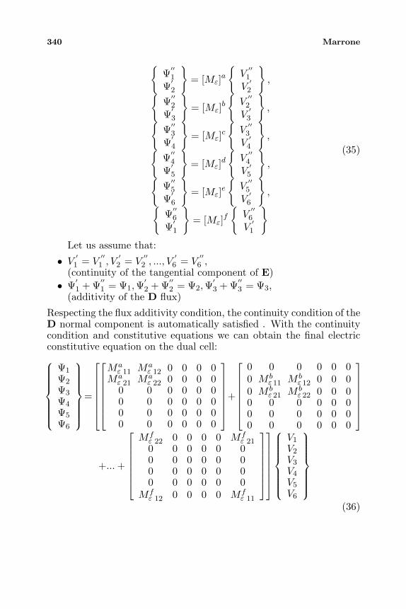
340 Marrone
Ψ′′1
Ψ′2
= [Mε]
a
V′′1
V′2
,
Ψ′′2
Ψ′3
= [Mε]
b
V′′2
V′3
,
Ψ′′3
Ψ′4
= [Mε]
c
V′′3
V′4
,
Ψ′′4
Ψ′5
= [Mε]
d
V′′4
V′5
,
Ψ′′5
Ψ′6
= [Mε]
e
V′′5
V′6
,
Ψ′′6
Ψ′1
= [Mε]
f
V′′6
V′1
(35)
Let us assume that:
• V′1 = V
′′1 , V
′2 = V
′′2 , ..., V
′6 = V
′′6 ,
(continuity of the tangential component of E)• Ψ
′1 + Ψ
′′1 = Ψ1,Ψ
′2 + Ψ
′′2 = Ψ2,Ψ
′3 + Ψ
′′3 = Ψ3,
(additivity of the D flux)
Respecting the flux additivity condition, the continuity condition of theD normal component is automatically satisfied . With the continuitycondition and constitutive equations we can obtain the final electricconstitutive equation on the dual cell:
Ψ1
Ψ2
Ψ3
Ψ4
Ψ5
Ψ6
=
Maε 11 Ma
ε 12 0 0 0 0Ma
ε 21 Maε 22 0 0 0 0
0 0 0 0 0 00 0 0 0 0 00 0 0 0 0 00 0 0 0 0 0
+
0 0 0 0 0 00 M b
ε 11 M bε 12 0 0 0
0 M bε 21 M b
ε 22 0 0 00 0 0 0 0 00 0 0 0 0 00 0 0 0 0 0
+... +
Mfε 22 0 0 0 0 Mf
ε 210 0 0 0 0 00 0 0 0 0 00 0 0 0 0 00 0 0 0 0 0
Mfε 12 0 0 0 0 Mf
ε 11
V1
V2
V3
V4
V5
V6
(36)
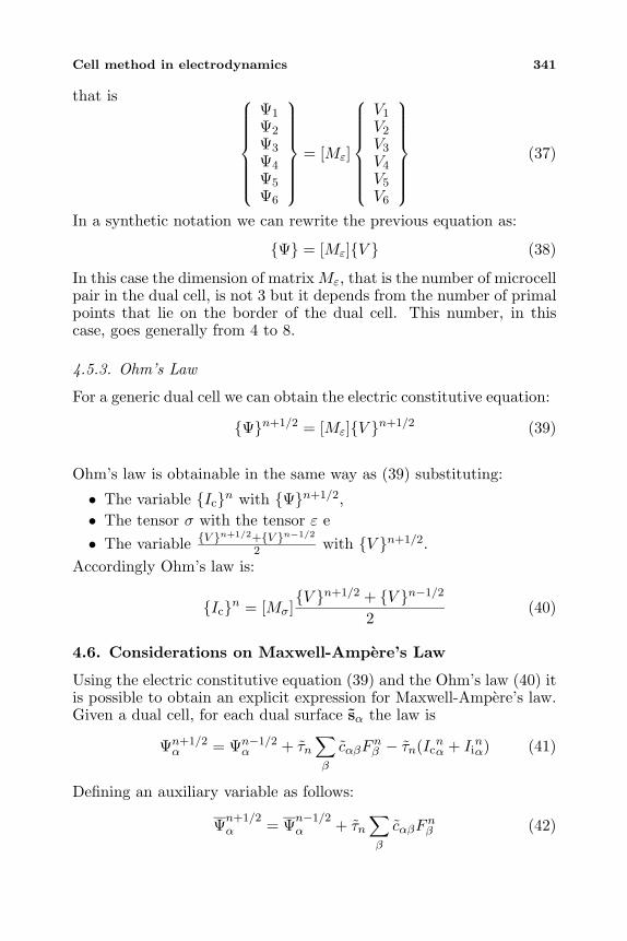
Cell method in electrodynamics 341
that is
Ψ1
Ψ2
Ψ3
Ψ4
Ψ5
Ψ6
= [Mε]
V1
V2
V3
V4
V5
V6
(37)
In a synthetic notation we can rewrite the previous equation as:
Ψ = [Mε]V (38)
In this case the dimension of matrix Mε, that is the number of microcellpair in the dual cell, is not 3 but it depends from the number of primalpoints that lie on the border of the dual cell. This number, in thiscase, goes generally from 4 to 8.
4.5.3. Ohm’s Law
For a generic dual cell we can obtain the electric constitutive equation:
Ψn+1/2 = [Mε]V n+1/2 (39)
Ohm’s law is obtainable in the same way as (39) substituting:
• The variable Icn with Ψn+1/2,• The tensor σ with the tensor ε e• The variable V
n+1/2+V n−1/2
2 with V n+1/2.Accordingly Ohm’s law is:
Icn = [Mσ]V n+1/2 + V n−1/2
2(40)
4.6. Considerations on Maxwell-Ampere’s Law
Using the electric constitutive equation (39) and the Ohm’s law (40) itis possible to obtain an explicit expression for Maxwell-Ampere’s law.Given a dual cell, for each dual surface sα the law is
Ψn+1/2α = Ψn−1/2
α + τn∑β
cαβFnβ − τn(Ic
nα + Ii
nα) (41)
Defining an auxiliary variable as follows:
Ψn+1/2α = Ψn−1/2
α + τn∑β
cαβFnβ (42)
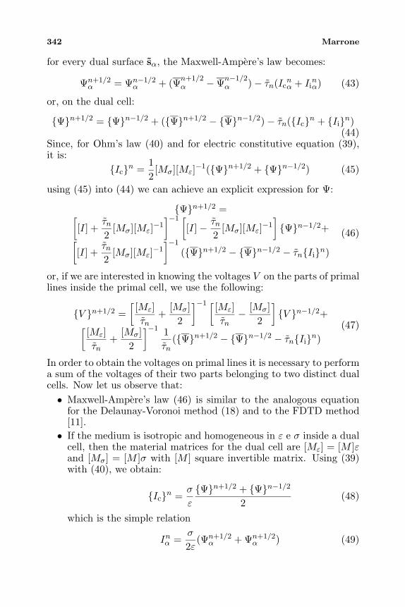
342 Marrone
for every dual surface sα, the Maxwell-Ampere’s law becomes:
Ψn+1/2α = Ψn−1/2
α + (Ψn+1/2α −Ψn−1/2
α )− τn(Icnα + Ii
nα) (43)
or, on the dual cell:
Ψn+1/2 = Ψn−1/2 + (Ψn+1/2 − Ψn−1/2)− τn(Icn + Iin)(44)
Since, for Ohm’s law (40) and for electric constitutive equation (39),it is:
Icn =12[Mσ][Mε]−1(Ψn+1/2 + Ψn−1/2) (45)
using (45) into (44) we can achieve an explicit expression for Ψ:
Ψn+1/2 =[[I] +
τn2
[Mσ][Mε]−1]−1 [
[I]− τn2
[Mσ][Mε]−1]Ψn−1/2+[
[I] +τn2
[Mσ][Mε]−1]−1
(Ψn+1/2 − Ψn−1/2 − τnIin)
(46)
or, if we are interested in knowing the voltages V on the parts of primallines inside the primal cell, we use the following:
V n+1/2 =[[Mε]τn
+[Mσ]
2
]−1 [[Mε]τn− [Mσ]
2
]V n−1/2+
[[Mε]τn
+[Mσ]
2
]−1 1τn
(Ψn+1/2 − Ψn−1/2 − τnIin)(47)
In order to obtain the voltages on primal lines it is necessary to performa sum of the voltages of their two parts belonging to two distinct dualcells. Now let us observe that:• Maxwell-Ampere’s law (46) is similar to the analogous equation
for the Delaunay-Voronoi method (18) and to the FDTD method[11].• If the medium is isotropic and homogeneous in ε e σ inside a dual
cell, then the material matrices for the dual cell are [Mε] = [M ]εand [Mσ] = [M ]σ with [M ] square invertible matrix. Using (39)with (40), we obtain:
Icn =σ
ε
Ψn+1/2 + Ψn−1/2
2(48)
which is the simple relation
Inα =σ
2ε(Ψn+1/2
α + Ψn+1/2α ) (49)
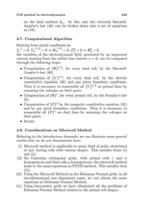
Cell method in electrodynamics 343
on the dual surfaces sα. In this case the vectorial Maxwell-Ampere’s law (46) can be broken down into a set of equationsas (18).
4.7. Computational Algorithm
Starting from initial conditions as:I−1α = 0, V −1/2
α = 0⇒ Ψ−1/2α = 0, F 0
β = 0⇒ Φ0β = 0
the variables of the electrodynamic field, generated by an impressedcurrent starting from the initial time instant n = 0, can be computedthrough the following steps:
• Computation of Ψ1/2, for every dual cell, by the Maxwell-Ampere’s law (46).
• Computation of V 1/2, for every dual cell, by the electricconstitutive equation (38) and any given boundary conditions.Then it is necessary to reassemble all V 1/2 on primal lines bysumming the voltages on their parts.
• Computation of Φ1, for every primal cell, by the Faraday’s law(6).• Computation of F1 by the magnetic constitutive equation (31)
and by any given boundary conditions. Then it is necessary toreassemble all F1 on dual lines by summing the voltages ontheir parts.
• Iterate
4.8. Considerations on Microcell Method
Referring to the introductory demands, we can illustrate some generalresults that we do not demonstrate here:
(i) Microcell method is applicable to many kind of grids, structuredor not, having cells with various shapes. This satisfies items (i)and (ii).
(ii) On Cartesian orthogonal grids, with primal cells ε and σhomogeneous and dual cells µ homogeneous, the microcell methodleads to the same equations as FDTD method. This satisfies item(iii).
(iii) Using the Microcell Method on the Delaunay-Voronoi grids, in alltwo-dimensional non degenerate cases, we can obtain the sameequations as Delaunay-Voronoi Method.
(iv) Using barycentric grids we have eliminated all the problems ofDelaunay-Voronoi Method related to the primal cell shapes.
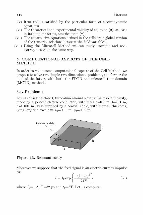
344 Marrone
(v) Item (iv) is satisfied by the particular form of electrodynamicequations.
(vi) The theoretical and experimental validity of equation (9), at leastin its simplest forms, satisfies item (v).
(vii) The constitutive equations defined in the cells are a global versionof the tensorial relations between the field variables.
(viii) Using the Microcell Method we can study isotropic and non-isotropic cases in the same way.
5. COMPUTATIONAL ASPECTS OF THE CELLMETHOD
In order to value some computational aspects of the Cell Method, wepropose to solve two simple two-dimensional problems, the former thedual of the latter, with both the FDTD and microcell time-domain(MCTD) methods.
5.1. Problem 1
Let us consider a closed, three-dimensional rectangular resonant cavity,made by a perfect electric conductor, with sizes a=0.1 m, b=0.1 m,h=0.001 m. It is supplied by a coaxial cable, with a small thickness,lying long the axes z in x0=0.02 m, y0=0.02 m.
Coaxial cable
a
b
h
Figure 13. Resonant cavity.
Moreover we suppose that the feed signal is an electric current impulseas:
I = I0 exp
−(t− t0)2
2T 2
(50)
where I0=1 A, T=32 ps and t0=3T. Let us compute:
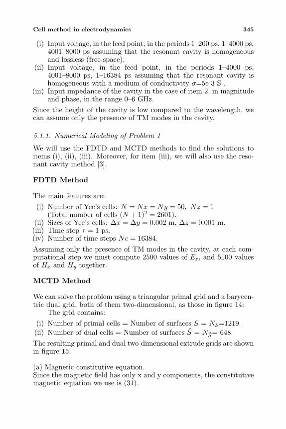
Cell method in electrodynamics 345
(i) Input voltage, in the feed point, in the periods 1–200 ps, 1–4000 ps,4001–8000 ps assuming that the resonant cavity is homogeneousand lossless (free-space).
(ii) Input voltage, in the feed point, in the periods 1–4000 ps,4001–8000 ps, 1–16384 ps assuming that the resonant cavity ishomogeneous with a medium of conductivity σ=5e-3 S .
(iii) Input impedance of the cavity in the case of item 2, in magnitudeand phase, in the range 0–6 GHz.
Since the height of the cavity is low compared to the wavelength, wecan assume only the presence of TM modes in the cavity.
5.1.1. Numerical Modeling of Problem 1
We will use the FDTD and MCTD methods to find the solutions toitems (i), (ii), (iii). Moreover, for item (iii), we will also use the reso-nant cavity method [3].
FDTD Method
The main features are:(i) Number of Yee’s cells: N = Nx = Ny = 50, Nz = 1
(Total number of cells (N + 1)2 = 2601).(ii) Sizes of Yee’s cells: ∆x = ∆y = 0.002 m, ∆z = 0.001 m.(iii) Time step τ = 1 ps.(iv) Number of time steps Nc = 16384.Assuming only the presence of TM modes in the cavity, at each com-putational step we must compute 2500 values of Ez, and 5100 valuesof Hx and Hy together.
MCTD Method
We can solve the problem using a triangular primal grid and a barycen-tric dual grid, both of them two-dimensional, as those in figure 14:
The grid contains:(i) Number of primal cells = Number of surfaces S = NS=1219.(ii) Number of dual cells = Number of surfaces S = NS= 648.The resulting primal and dual two-dimensional extrude grids are shownin figure 15.
(a) Magnetic constitutive equation.Since the magnetic field has only x and y components, the constitutivemagnetic equation we use is (31).
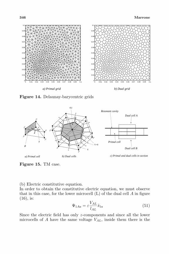
346 Marrone
0 0.01 0.02 0.03 0.04 0.05 0.06 0.07 0.08 0.09 0.10
0.01
0.02
0.03
0.04
0.05
0.06
0.07
0.08
0.09
0.1
0 0.01 0.02 0.03 0.04 0.05 0.06 0.07 0.08 0.09 0.10
0.01
0.02
0.03
0.04
0.05
0.06
0.07
0.08
0.09
0.1
a) Primal grid b) Dual grid
Figure 14. Delaunay-barycentric grids
a) Primal cell
Primal cell
b) Dual cells
Dual cell B
Dual cell A
Resonant cavity
c) Primal and dual cells in section
P
P
P
P
PP
P
P
P
P
Φ
V
V=0F
Ψ,I
Figure 15. TM case.
(b) Electric constitutive equation.In order to obtain the constitutive electric equation, we must observethat in this case, for the lower microcell (L) of the dual cell A in figure(16), is:
Ψ1Aa = εVALlAL
s1a (51)
Since the electric field has only z-components and since all the lowermicrocells of A have the same voltage VAL, inside them there is the
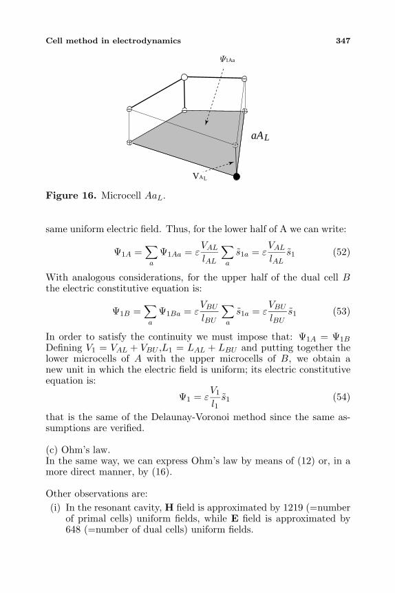
Cell method in electrodynamics 347
Ψ1Aa
VAL
aAL
Figure 16. Microcell AaL.
same uniform electric field. Thus, for the lower half of A we can write:
Ψ1A =∑a
Ψ1Aa = εVALlAL
∑a
s1a = εVALlAL
s1 (52)
With analogous considerations, for the upper half of the dual cell Bthe electric constitutive equation is:
Ψ1B =∑a
Ψ1Ba = εVBUlBU
∑a
s1a = εVBUlBU
s1 (53)
In order to satisfy the continuity we must impose that: Ψ1A = Ψ1B
Defining V1 = VAL + VBU ,L1 = LAL + LBU and putting together thelower microcells of A with the upper microcells of B, we obtain anew unit in which the electric field is uniform; its electric constitutiveequation is:
Ψ1 = εV1
l1s1 (54)
that is the same of the Delaunay-Voronoi method since the same as-sumptions are verified.
(c) Ohm’s law.In the same way, we can express Ohm’s law by means of (12) or, in amore direct manner, by (16).
Other observations are:(i) In the resonant cavity, H field is approximated by 1219 (=number
of primal cells) uniform fields, while E field is approximated by648 (=number of dual cells) uniform fields.
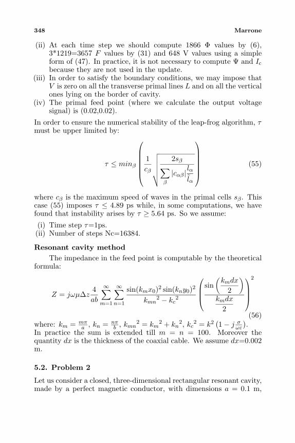
348 Marrone
(ii) At each time step we should compute 1866 Φ values by (6),3*1219=3657 F values by (31) and 648 V values using a simpleform of (47). In practice, it is not necessary to compute Ψ and Ic
because they are not used in the update.(iii) In order to satisfy the boundary conditions, we may impose that
V is zero on all the transverse primal lines L and on all the verticalones lying on the border of cavity.
(iv) The primal feed point (where we calculate the output voltagesignal) is (0.02,0.02).
In order to ensure the numerical stability of the leap-frog algorithm, τmust be upper limited by:
τ ≤ minβ
1cβ
√√√√√√2sβ∑
β
|cαβ |lα
lα
(55)
where cβ is the maximum speed of waves in the primal cells sβ. Thiscase (55) imposes τ ≤ 4.89 ps while, in some computations, we havefound that instability arises by τ ≥ 5.64 ps. So we assume:
(i) Time step τ=1ps.(ii) Number of steps Nc=16384.
Resonant cavity methodThe impedance in the feed point is computable by the theoretical
formula:
Z = jωµ∆z4ab
∞∑m=1
∞∑n=1
sin(kmx0)2 sin(kny0)2
kmn2 − kc
2
sin(kmdx
2
)
kmdx
2
2
(56)where: km = mπ
a , kn = nπb , kmn2 = km
2 + kn2, kc2 = k2
(1− j σ
ωε
).
In practice the sum is extended till m = n = 100. Moreover thequantity dx is the thickness of the coaxial cable. We assume dx=0.002m.
5.2. Problem 2
Let us consider a closed, three-dimensional rectangular resonant cavity,made by a perfect magnetic conductor, with dimensions a = 0.1 m,
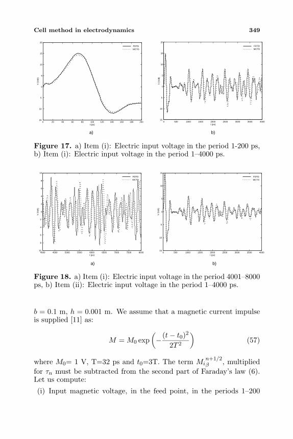
Cell method in electrodynamics 349
0 20 40 60 80 100 120 140 160 180 20015
10
5
0
5
10
15
20
t (ps)
V (
Vol
t)
MCTDFDTD
0 500 1000 1500 2000 2500 3000 3500 400015
10
5
0
5
10
15
20
t (ps)
MCTDFDTD
V (
Vol
t)
a) b)
Figure 17. a) Item (i): Electric input voltage in the period 1-200 ps,b) Item (i): Electric input voltage in the period 1–4000 ps.
4000 4500 5000 5500 6000 6500 7000 7500 800010
8
6
4
2
0
2
4
6
8
10
t (ps)
MCTDFDTD
V (
Vol
t)
0 500 1000 1500 2000 2500 3000 3500 400015
10
5
0
5
10
15
t (ps)
MCTDFDTD
V (
Vol
t)
a) b)
Figure 18. a) Item (i): Electric input voltage in the period 4001–8000ps, b) Item (ii): Electric input voltage in the period 1–4000 ps.
b = 0.1 m, h = 0.001 m. We assume that a magnetic current impulseis supplied [11] as:
M = M0 exp(−(t− t0)2
2T 2
)(57)
where M0= 1 V, T=32 ps and t0=3T. The term Min+1/2β , multiplied
for τn must be subtracted from the second part of Faraday’s law (6).Let us compute:
(i) Input magnetic voltage, in the feed point, in the periods 1–200
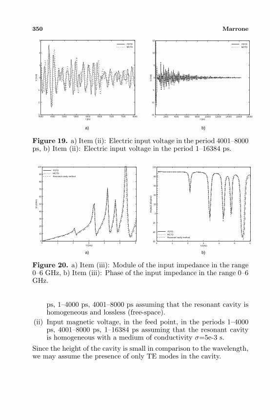
350 Marrone
4000 4500 5000 5500 6000 6500 7000 7500 80003
2
1
0
1
2
3
t (ps)
MCTDFDTD
V (
Vol
t)
0 2000 4000 6000 8000 10000 12000 14000 16000 1800015
10
5
0
5
10
15
t (ps)
MCTDFDTD
V (
Vol
t)
a) b)
Figure 19. a) Item (ii): Electric input voltage in the period 4001–8000ps, b) Item (ii): Electric input voltage in the period 1–16384 ps.
0 1 2 3 4 5 60
10
20
30
40
50
60
70
80
90
100
f (GHz)
|Z| (
Ohm
)
MCTD
Resonant cavity method
FDTD
0 1 2 3 4 5 660
40
20
0
20
40
60
80
100
f (GHz)
Ang
le(Z
) (D
egre
e)
MCTDFDTD
Resonant cavity method
a) b)
Figure 20. a) Item (iii): Module of the input impedance in the range0–6 GHz, b) Item (iii): Phase of the input impedance in the range 0–6GHz.
ps, 1–4000 ps, 4001–8000 ps assuming that the resonant cavity ishomogeneous and lossless (free-space).
(ii) Input magnetic voltage, in the feed point, in the periods 1–4000ps, 4001–8000 ps, 1–16384 ps assuming that the resonant cavityis homogeneous with a medium of conductivity σ=5e-3 s.
Since the height of the cavity is small in comparison to the wavelength,we may assume the presence of only TE modes in the cavity.
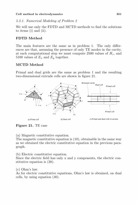
Cell method in electrodynamics 351
5.2.1. Numerical Modeling of Problem 2
We will use only the FDTD and MCTD methods to find the solutionsto items (i) and (ii).
FDTD Method
The main features are the same as in problem 1. The only differ-ences are that, assuming the presence of only TE modes in the cavity,at each computational step we must compute 2500 values of Hz, and5100 values of Ex and Ey together.
MCTD Method
Primal and dual grids are the same as problem 1 and the resultingtwo-dimensional extrude cells are shown in figure 21.
a) Prima cell b) Dual cell c) Primal and dual cells in section
P
P
P
P
P
P
P
P
P
P
Φ
V=0
V=0
V
F=0
F
Ψ,I
Primal cell
Primal cellDual cell
Resonant cavity
Figure 21. TE case
(a) Magnetic constitutive equation.The magnetic constitutive equation is (10), obtainable in the same wayas we obtained the electric constitutive equation in the previous para-graph.
(b) Electric constitutive equation.Since the electric field has only x and y components, the electric con-stitutive equation is (38).
(c) Ohm’s law.As for electric constitutive equations, Ohm’s law is obtained, on dualcells, by using equation (40).
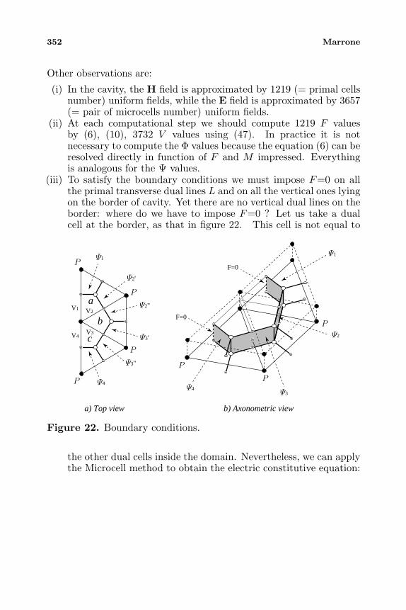
352 Marrone
Other observations are:
(i) In the cavity, the H field is approximated by 1219 (= primal cellsnumber) uniform fields, while the E field is approximated by 3657(= pair of microcells number) uniform fields.
(ii) At each computational step we should compute 1219 F valuesby (6), (10), 3732 V values using (47). In practice it is notnecessary to compute the Φ values because the equation (6) can beresolved directly in function of F and M impressed. Everythingis analogous for the Ψ values.
(iii) To satisfy the boundary conditions we must impose F=0 on allthe primal transverse dual lines L and on all the vertical ones lyingon the border of cavity. Yet there are no vertical dual lines on theborder: where do we have to impose F=0 ? Let us take a dualcell at the border, as that in figure 22. This cell is not equal to
P
P
P
P
P
P
P
Ψ3
Ψ2
Ψ1Ψ1
Ψ4
Ψ3"
Ψ3'
Ψ2"
Ψ2'
F=0
F=0
Ψ4
V3
V2V1
V4
b) Axonometric view
a
b
c
a) Top view
Figure 22. Boundary conditions.
the other dual cells inside the domain. Nevertheless, we can applythe Microcell method to obtain the electric constitutive equation:
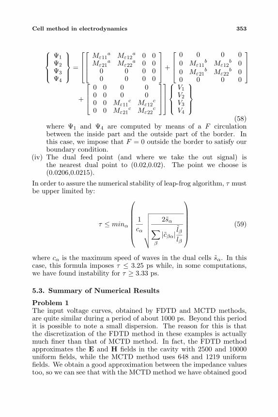
Cell method in electrodynamics 353
Ψ1
Ψ2
Ψ3
Ψ4
=
Mε11a Mε12
a 0 0Mε21
a Mε22a 0 0
0 0 0 00 0 0 0
+
0 0 0 00 Mε11
b Mε12b 0
0 Mε21b Mε22
b 00 0 0 0
+
0 0 0 00 0 0 00 0 Mε11
c Mε12c
0 0 Mε21c Mε22
c
V1
V2
V3
V4
(58)where Ψ1 and Ψ4 are computed by means of a F circulationbetween the inside part and the outside part of the border. Inthis case, we impose that F = 0 outside the border to satisfy ourboundary condition.
(iv) The dual feed point (and where we take the out signal) isthe nearest dual point to (0.02,0.02). The point we choose is(0.0206,0.0215).
In order to assure the numerical stability of leap-frog algorithm, τ mustbe upper limited by:
τ ≤ minα
1cα
√√√√√√√2sα
∑β
|cβα|lβlβ
(59)
where cα is the maximum speed of waves in the dual cells sα. In thiscase, this formula imposes τ ≤ 3.25 ps while, in some computations,we have found instability for τ ≥ 3.33 ps.
5.3. Summary of Numerical Results
Problem 1The input voltage curves, obtained by FDTD and MCTD methods,are quite similar during a period of about 1000 ps. Beyond this periodit is possible to note a small dispersion. The reason for this is thatthe discretization of the FDTD method in these examples is actuallymuch finer than that of MCTD method. In fact, the FDTD methodapproximates the E and H fields in the cavity with 2500 and 10000uniform fields, while the MCTD method uses 648 and 1219 uniformfields. We obtain a good approximation between the impedance valuestoo, so we can see that with the MCTD method we have obtained good
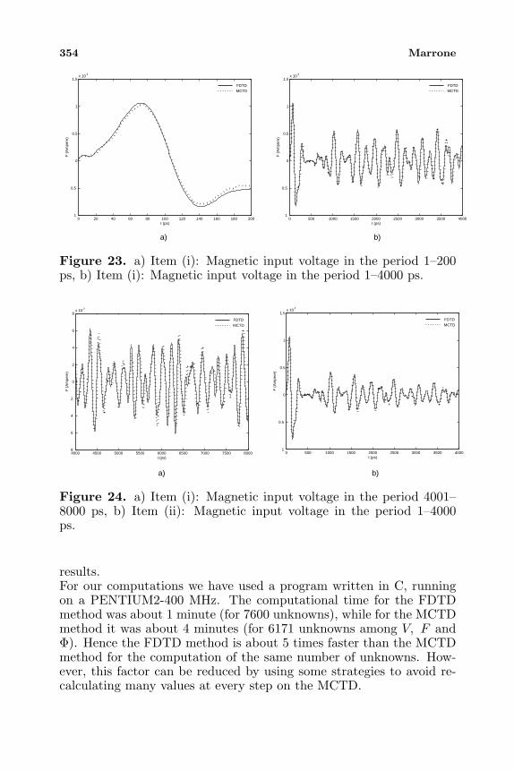
354 Marrone
0 20 40 60 80 100 120 140 160 180 2001
0.5
0
0.5
1
1.5x 10
4
F (
Am
pere
)
t (ps)
MCTDFDTD
0 500 1000 1500 2000 2500 3000 3500 40001
0.5
0
0.5
1
1.5x 10
4
F (
Am
pere
)
t (ps)
MCTDFDTD
a) b)
Figure 23. a) Item (i): Magnetic input voltage in the period 1–200ps, b) Item (i): Magnetic input voltage in the period 1–4000 ps.
4000 4500 5000 5500 6000 6500 7000 7500 80008
6
4
2
0
2
4
6
8x 10
5
F (
Am
pere
)
t (ps)
MCTDFDTD
0 500 1000 1500 2000 2500 3000 3500 40001
0.5
0
0.5
1
1.5x 10
4
F (
Am
pere
)
t (ps)
MCTDFDTD
a) b)
Figure 24. a) Item (i): Magnetic input voltage in the period 4001–8000 ps, b) Item (ii): Magnetic input voltage in the period 1–4000ps.
results.For our computations we have used a program written in C, runningon a PENTIUM2-400 MHz. The computational time for the FDTDmethod was about 1 minute (for 7600 unknowns), while for the MCTDmethod it was about 4 minutes (for 6171 unknowns among V, F andΦ). Hence the FDTD method is about 5 times faster than the MCTDmethod for the computation of the same number of unknowns. How-ever, this factor can be reduced by using some strategies to avoid re-calculating many values at every step on the MCTD.
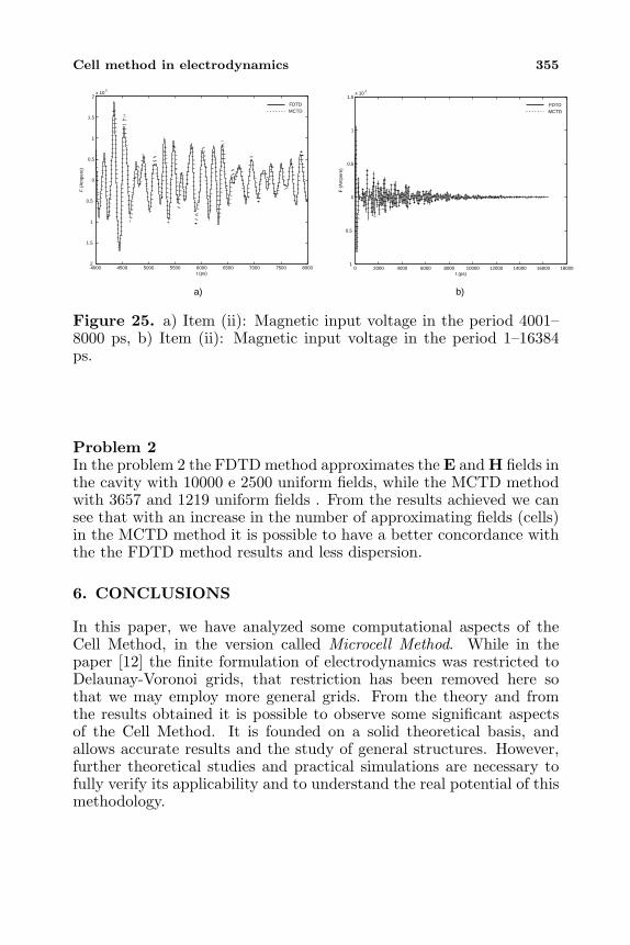
Cell method in electrodynamics 355
4000 4500 5000 5500 6000 6500 7000 7500 80002
1.5
1
0.5
0
0.5
1
1.5
2x 10
5
F (
Am
pere
)
t (ps)
MCTDFDTD
0 2000 4000 6000 8000 10000 12000 14000 16000 180001
0.5
0
0.5
1
1.5x 10
4
F (
Am
pere
)
t (ps)
MCTDFDTD
a) b)
Figure 25. a) Item (ii): Magnetic input voltage in the period 4001–8000 ps, b) Item (ii): Magnetic input voltage in the period 1–16384ps.
Problem 2In the problem 2 the FDTD method approximates the E and H fields inthe cavity with 10000 e 2500 uniform fields, while the MCTD methodwith 3657 and 1219 uniform fields . From the results achieved we cansee that with an increase in the number of approximating fields (cells)in the MCTD method it is possible to have a better concordance withthe the FDTD method results and less dispersion.
6. CONCLUSIONS
In this paper, we have analyzed some computational aspects of theCell Method, in the version called Microcell Method. While in thepaper [12] the finite formulation of electrodynamics was restricted toDelaunay-Voronoi grids, that restriction has been removed here sothat we may employ more general grids. From the theory and fromthe results obtained it is possible to observe some significant aspectsof the Cell Method. It is founded on a solid theoretical basis, andallows accurate results and the study of general structures. However,further theoretical studies and practical simulations are necessary tofully verify its applicability and to understand the real potential of thismethodology.
356 Marrone
REFERENCES
1. Pauli, W., Elettrodinamica, (translation of Vorlesung Elektrody-namik), Boringhieri (ed.), 1964.
2. Yee, K. S., “Numerical solution of initial boundary valueproblems involving Maxwell’s equations in isotropic media,” IEEETransactions on Antennas and Propagation, Vol. 14, 302–307,1966.
3. Carver, K. R. and J. W. Mink, “Microstrip antenna technology,”IEEE Transactions on Antennas and Propagation, Vol. 29, 2–24,1981.
4. Holland, R., “Finite difference solutions of Maxwell’s equationsin generalized nonorthogonal coordinates,” IEEE Transactions onNuclear Science, Vol. 30, No. 6, 4689–4591, 1983.
5. Fusco, M., “FDTD algorithm in curvilinear coordinates,” IEEETransactions on Antennas and Propagation, Vol. 38, No. 1, 76–89, 1990.
6. Lee, J. F., R. Palandech, and R. Mittra, “Modeling three-dimensional discontinuites in waveguides using nonorthogonalFDTD algorithm,” IEEE Transactions on Microwave andTechniques, Vol. 40, No. 2, 346–352, 1992.
7. Lee, C. F., B. J. McCartin, R. T. Shin, and J. A. Kong,“A triangular-grid finite-difference time-domain method forelectromagnetic scattering problems,” Journal of ElectromagneticsWaves and Applications, Vol. 8, No. 4, 449–470, 1994.
8. Madsen, N. K., “Divergence preserving discrete surface integralmethods for Maxwell’s curl equations using non-orthogonalunstructured grids,” Journal of Computational Physics, Vol. 119,34–45, 1995.
9. Hano, M. and T. Itoh, “Three-dimensional time-domain methodfor solving Maxwell’s equations based on circumcenters ofelements,” IEEE Transactions on Magnetics, Vol. 32, No. 3, 946–949, 1996.
10. Schuhmann, R. and T. Weiland, “FDTD on nonorthogonalgrids with triangular fillings,” IEEE Transactions on Magnetics,Vol. 35, No. 3, 1470–1473, 1999.
11. Taflove, A., Computational Electrodynamics: The Finite-Difference Time-Domain Method, Artech House, 1995.
12. Tonti, E., “Finite formulation of the electromagnetic field,” thisvolume.
Progress In Electromagnetics Research, PIER 32, 357–381, 2001
FREQUENCY DOMAIN ANALYSIS OF WAVEGUIDESAND RESONATORS WITH FIT ONNON-ORTHOGONAL TRIANGULAR GRIDS
U. van Rienen
Institute of General Electrical EngineeringFaculty of Engineering, Rostock UniversityD-18051 Rostock, Germany
Abstract—The focus of this paper is on the solution of Maxwell’sequations for time-harmonic fields on triangular, possibly non-orthogonal meshes. The method is based on the well-known FiniteIntegration Technique (FIT) [33, 35] which is a proven consistentdiscretization method for the computation of electromagnetic fields.FIT on triangular grids was first introduced in [29, 31] for eigenvalueproblems arising in the design of accelerator components and dielectricloaded waveguides. For many technical applications the 2D simulationon a triangular grid combines the advantages of FIT, as e.g. theconsistency of the method or the numerical advantage of bandedsystem matrices, with the geometrical flexibility of non-coordinategrids. The FIT-discretization on non-orthogonal 2D grids has closerelations [26] to the Nedelec elements [14, 15] or edge elements in theFinite Element Method.
1 Introduction
2 FIT-Discretization on a Triangular Grid2.1 The Triangular Grid and its Dual Grid2.2 Continuity Conditions for the Non-Orthogonal Case2.3 State Variables and Discrete Operators for the Triangu-
lar Grid2.4 Error Behaviour2.5 Relation to Mixed Finite Elements
3 Examples3.1 Tuned Multicell Cavity3.2 Dispersion Relation for Loaded Waveguide
358 van Rienen
3.3 Circular Waveguide with Capacitive Load3.4 Parameter Study for Loaded Ridged Waveguide
4 Conclusion and outlook
References
1. INTRODUCTION
The most important class of methods for numerical field calculationdeals with local difference equations obtained after suitable discretiza-tion. Well-known examples are the Finite Difference Method (FD)and the Finite Element Method (FEM). The Finite Integration Tech-nique [33, 35, 36], shortly FIT, presents a discretization consistent withMaxwell’s equations, i.e., the resulting discrete solutions reflect the an-alytical properties of the continuous solutions. The Finite IntegrationTechnique can best be described as a Finite Volume method. It hasbeen developed specifically for the solution of Maxwell’s equations.The goal of this development was the ability to solve numerically thecomplete system of Maxwell’s equations in full generality.
Regard Maxwell’s equations which can either be written in integralform or in differential form
∮∂A
E · ds = −∫A
∂ B
∂t· d A ⇐⇒ curl E = −∂ B
∂t∮∂A
H · ds =∫A(∂ D
∂t+ J) · d A ⇐⇒ curl H =
∂ D
∂t+ J
∮∂V
D · d A =∫Vρ · dV ⇐⇒ div D = ρ
∮∂V
B · d A = 0 ⇐⇒ div B = 0
where A is any given surface and V any given volume.The Finite Integration Technique yields an exact representation
of Maxwell’s equations in integral form onto a grid duplet (G, G).The FIT grid duplet (G, G) is not coordinate-bounded, not necessarilyorthogonal, not necessarily regular. Yee’s FDTD-method [40] (1966)with the “Leap Frog”-scheme is a predecessor of FIT in FiniteDifference Time Domain (FDTD stands for Finite Difference TimeDomain). The feature of Yee’s method is that it evaluates Maxwell’sequations for both electromagnetic fields (not just the electric field) and
Frequency domain analysis with FIT 359
that the electric and magnetic field components were allocated on twostaggered grids. In 1977, Weiland [33] generalized the FDTD-methodto a general numerical method for all electrodynamics. In fact, FIT isnot restricted to electrodynamics only but is also a suitable numericalmethod for other subjects. For example, FIT was recently applied inacoustics [39], elastodynamics [12, 2] and temperature problems [17, 16]and for coupled problems [28, 1].
The Finite Integration Technique makes only some usualidealizations concerning the materials: The materials of the givenobjects have to be piecewise linear, homogeneous, and isotropic sothat the subdomains with constant material parameters (ε, µ, κ) are atleast as big as the elementary volumes used.
The discretization of Maxwell’s equations, i.e., the fieldcomputation in a finite number of discrete points, gives adecomposition of the solution space into grid cells. The first steptowards that goal is to define a finite volume Ω, the calculation domain.Now, cover Ω with a grid G. As an example, we can consider a simpleCartesian coordinate grid. It has to be stressed at this point, however,that a FIT grid G is defined in much more generality and that itsdefinition also includes non-coordinate grids as well as non-orthogonalgrids (cf. section 2 and [31, 27] or e.g. [9, 10, 23, 20, 21]). For the simpleCartesian coordinate grid, we will explain very briefly the derivationof the Maxwell Grid Equations. Further details can be found e.g. in[37, 6, 27].
Definition 1. A FIT grid G is defined as:- G ∈ R3 (R2) simply connected- elementary volumes V = V1, ..., VnV with G =
⋃Vi, Vi = ;
- elementary areas A = A1, ..., AnA with Ai :=⋂
Vi- elementary lines L = L1, ..., LnL with Li :=
⋂Ai
- (grid) points P = P1, ..., PnP with Pi :=⋂
Li
An elementary volume Vi (FIT cell) for the simplest case is shownin Fig. 1. Next, state variables [34] are introduced on the grid G:
Definition 2. The electric (grid-)voltage ei :=∫Li
E · ds is assignedto each elementary line Li as state variable.The magnetic (grid-)flux bi :=
∫Ai
B · d A normal to the elementaryarea Ai is assigned as state variable to each elementary area Ai.
After appropriate numbering of the points of the grid, the statevariables ei and bi, i = 1, . . . , 3N can be stored in vectors e and b and
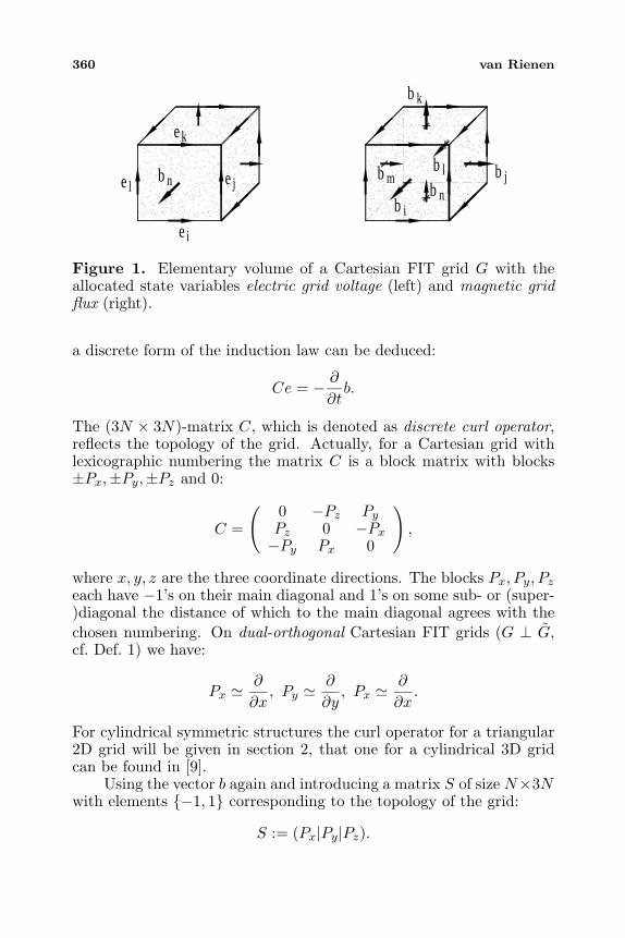
360 van Rienen
e
k
lbe n
e
i
jeb
b i
b mn
blbj
b k
Figure 1. Elementary volume of a Cartesian FIT grid G with theallocated state variables electric grid voltage (left) and magnetic gridflux (right).
a discrete form of the induction law can be deduced:
Ce = − ∂
∂tb.
The (3N × 3N)-matrix C, which is denoted as discrete curl operator,reflects the topology of the grid. Actually, for a Cartesian grid withlexicographic numbering the matrix C is a block matrix with blocks±Px,±Py,±Pz and 0:
C =
( 0 −Pz Py
Pz 0 −Px
−Py Px 0
),
where x, y, z are the three coordinate directions. The blocks Px, Py, Pz
each have −1’s on their main diagonal and 1’s on some sub- or (super-)diagonal the distance of which to the main diagonal agrees with thechosen numbering. On dual-orthogonal Cartesian FIT grids (G ⊥ G,cf. Def. 1) we have:
Px ∂
∂x, Py
∂
∂y, Px
∂
∂x.
For cylindrical symmetric structures the curl operator for a triangular2D grid will be given in section 2, that one for a cylindrical 3D gridcan be found in [9].
Using the vector b again and introducing a matrix S of size N×3Nwith elements −1, 1 corresponding to the topology of the grid:
S := (Px|Py|Pz).
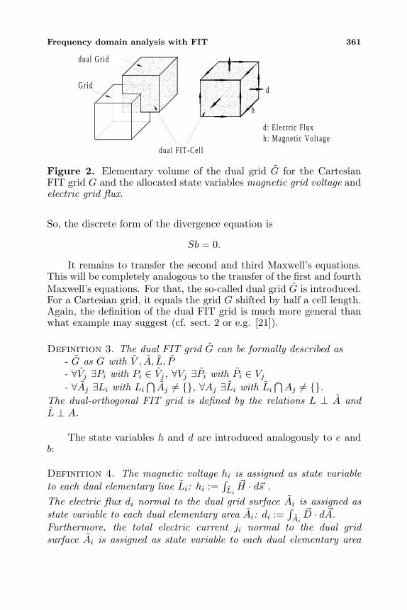
Frequency domain analysis with FIT 361
dua l Gr id
G r i d
dua l F IT-Ce l lh : Magne t i c Vo l t aged: Elec t r ic F lux
h
d
Figure 2. Elementary volume of the dual grid G for the CartesianFIT grid G and the allocated state variables magnetic grid voltage andelectric grid flux.
So, the discrete form of the divergence equation is
Sb = 0.
It remains to transfer the second and third Maxwell’s equations.This will be completely analogous to the transfer of the first and fourthMaxwell’s equations. For that, the so-called dual grid G is introduced.For a Cartesian grid, it equals the grid G shifted by half a cell length.Again, the definition of the dual FIT grid is much more general thanwhat example may suggest (cf. sect. 2 or e.g. [21]).
Definition 3. The dual FIT grid G can be formally described as- G as G with V , A, L, P- ∀Vj ∃Pi with Pi ∈ Vj, ∀Vj ∃Pi with Pi ∈ Vj- ∀Aj ∃Li with Li
⋂Aj = , ∀Aj ∃Li with Li
⋂Aj = .
The dual-orthogonal FIT grid is defined by the relations L ⊥ A andL ⊥ A.
The state variables h and d are introduced analogously to e andb:
Definition 4. The magnetic voltage hi is assigned as state variableto each dual elementary line Li: hi :=
∫Li
H · ds .The electric flux di normal to the dual grid surface Ai is assigned asstate variable to each dual elementary area Ai: di :=
∫Ai
D · d A.Furthermore, the total electric current ji normal to the dual gridsurface Ai is assigned as state variable to each dual elementary area
362 van Rienen
Ai: ji :=∫Ai
J · d A.The discrete charges qi (allocated in Pi on G) are assigned as statevariables to each dual elementary volume Vi: qi :=
∫Vi
ρdV.
The values of the state variables are stored in topological matricesC and S analogous to C and S. Thus, the discrete form of Ampere’slaw is
Ch =∂
∂td + j
and Coulomb’s law isSd = q.
To summarize the above, let us formally define the Maxwell GridEquations. It should be emphasized that no approximations have beenmade so far. Only when the material equations are transferred to thegrid space, FIT will require some approximations.
Ce = −b
Ch = d + j (1)Sb = 0Sd = q
Because of its consistency and generality this system is denoted asMaxwell-Grid-Equations. The operators C, C, S and S can beinterpreted as discrete curl operators C, C, discrete divergence S, Sand discrete gradient operators −ST ,−ST . The characteristics of theFinite Integration Technique are not given here. They can be found in[38, 11, 5] or [27].
Until now, no approximations have been used at all. They will benecessary after the transfer of the material equations to the grid space.The state variables di and ei (respectively bi and hi) are each allocatedat the same points. There is an analogue of the material equationsrelating them to each other. In order to find that analogue of thematerial equations, the grid flux is divided by the grid voltage. Theratios di/ei and bi/hi (ji/ei, respectively) then will be approximatedby averaging the corresponding material parameters. The averagedquantities are then combined in the so-called material matrices Dε, Dµ
and Dκ. A detailed description of this approximation can be found in[9, 6, 37]. We follow the formulation in [9]:
Definition 5. The elementary areas Ai and the corresponding dualelementary lines Li shall each be coordinate planes resp. coordinate
Frequency domain analysis with FIT 363
lines of a local orthogonal coordinate system which is differentiabletwice with respect to its Cartesian representation. The dual grid lineLi intersects the area Ai in its local middle point and vice versa. Thepermeability operator is then given by
Dµ,i =
∫Lm
∫Ln
dA∫Li
1µds
.
The (dual) elementary areas Ai and the corresponding elementary linesLi shall each be coordinate planes resp. coordinate lines of a localorthogonal coordinate system which is differentiable twice with respectto its Cartesian representation. The grid line Li intersects the area Ai
in its local middle point and vice versa. The permittivity operator isthen given by
Dε,i =
∫Lm
∫Ln
εdA∫Li
ds.
Thus, the construction of Dµ,i is based on lengthwise averaging.Its error is linear with respect to the energy norm if Ai representsa border of different permeabilities, otherwise it is quadratic. Theconstruction of Dε,i is based on areawise averaging. Its error is linearwith respect to the energy norm if Li borders different permittivitiesor permeabilities, otherwise it is quadratic.
Defining the conductivity operator Dκ in analogy, thus thefollowing transfer of the electromagnetic material equations to the gridspace results with diagonal material operators Dε, Dµ, Dκ:
D = ε E → d = DεeB = µ H → b = DµhJL = κE → jl = Dκe
Finally, boundary equations at ∂G are needed. Dirichlet and Neumannboundary conditions can be implemented in a FIT-scheme in a verynatural way, others like open (absorbing), periodic or waveguideboundary conditions have also been realized (see e.g. [37, 9, 5]).
Non-coordinate and non-orthogonal meshes offer an enhancedflexibility with regard to the spatial discretization of the field equations.Here, with a “coordinate mesh” a mesh is meant where the grid planesare coordinate planes in one of the usual coordinate systems as e.g. theCartesian or cylindrical coordinate system. The triangular grids whichare subject of this paper are an example for a ”non-coordinate mesh”.In the eighties when mainframes were the computers at hand allowing
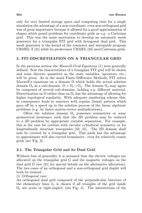
364 van Rienen
only for very limited storage space and computing time for a singlesimulation the advantage of a non-coordinate, even non-orthogonal gridwas of great importance because it allowed for a good approximation ofshapes which posed problems for coordinate grids as e.g. a Cartesiangrid. This was the main motivation to develop an automatic meshgenerator for a triangular FIT grid with hexagonal dual grid. Thismesh generator is the kernel of the resonator and waveguide programURMEL-T [31] while its predecessor URMEL [33] used Cartesian grids.
2. FIT-DISCRETIZATION ON A TRIANGULAR GRID
In the previous section the Maxwell-Grid-Equations (1) were generallydefined. Now the characteristics of a triangular FIT grid will be shownand some discrete quantities as the state variables, operators, etc.,will be given. As in the usual Finite Difference Methods, FIT solvesMaxwell’s equations on a domain Ω which holds the actual solutiondomain Ωs as a sub-domain: Ω = Ωs ∪Ωo. The domain Ωs may againbe composed of several sub-domains, holding e.g. different material.Discretization on Ω rather than on Ωs has the advantage of allowing forhigher topological regularity. With adequate numbering scheme this,in consequence leads to matrices with regular (band) pattern whichpays off by a speed up in the solution process of the linear algebraicproblems (e.g. by faster matrix-vector multiplications).
Often the solution domain Ωs possesses symmetries or somegeometrical invariance such that the 3D problem may be reducedto a 2D problem by appropriate variable separation. For example,this is the case for cavities with circular cylindrical symmetry or forlongitudinally invariant waveguides [33, 31]. The 2D domain shallnow be covered by a triangular grid. This mesh has the advantageto approximate well also curved boundaries - even for relatively coarsegrids (see Fig. 3).
2.1. The Triangular Grid and its Dual Grid
Without loss of generality it is assumed that the electric voltages areallocated on the triangular grid G and the magnetic voltages on thedual grid G (see [31] for special details on the alternative allocation).The two cases of an orthogonal and a non-orthogonal grid duplet willboth be treated:(i) Orthogonal case:An orthogonal dual grid composed of the perpendicular bisectors ofthe elementary lines Li is chosen if all triangles of the grid insideΩs are acute or right-angled, (see Fig. 4). The intersections of the
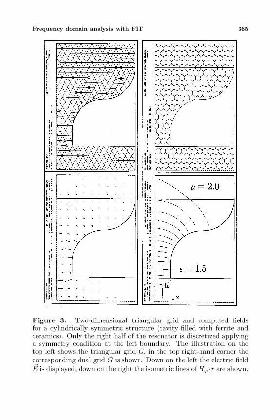
Frequency domain analysis with FIT 365
Figure 3. Two-dimensional triangular grid and computed fieldsfor a cylindrically symmetric structure (cavity filled with ferrite andceramics). Only the right half of the resonator is discretized applyinga symmetry condition at the left boundary. The illustration on thetop left shows the triangular grid G, in the top right-hand corner thecorresponding dual grid G is shown. Down on the left the electric fieldE is displayed, down on the right the isometric lines of Hϕ ·r are shown.
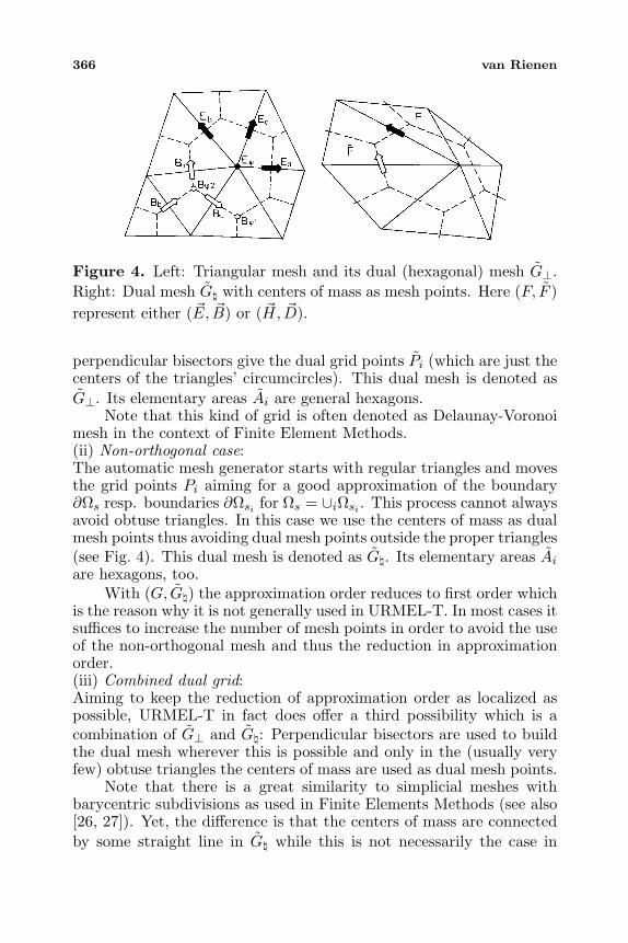
366 van Rienen
Figure 4. Left: Triangular mesh and its dual (hexagonal) mesh G⊥.Right: Dual mesh G with centers of mass as mesh points. Here (F, F )represent either ( E, B) or ( H, D).
perpendicular bisectors give the dual grid points Pi (which are just thecenters of the triangles’ circumcircles). This dual mesh is denoted asG⊥. Its elementary areas Ai are general hexagons.
Note that this kind of grid is often denoted as Delaunay-Voronoimesh in the context of Finite Element Methods.(ii) Non-orthogonal case:The automatic mesh generator starts with regular triangles and movesthe grid points Pi aiming for a good approximation of the boundary∂Ωs resp. boundaries ∂Ωsi for Ωs = ∪iΩsi . This process cannot alwaysavoid obtuse triangles. In this case we use the centers of mass as dualmesh points thus avoiding dual mesh points outside the proper triangles(see Fig. 4). This dual mesh is denoted as G. Its elementary areas Ai
are hexagons, too.With (G, G) the approximation order reduces to first order which
is the reason why it is not generally used in URMEL-T. In most cases itsuffices to increase the number of mesh points in order to avoid the useof the non-orthogonal mesh and thus the reduction in approximationorder.(iii) Combined dual grid:Aiming to keep the reduction of approximation order as localized aspossible, URMEL-T in fact does offer a third possibility which is acombination of G⊥ and G: Perpendicular bisectors are used to buildthe dual mesh wherever this is possible and only in the (usually veryfew) obtuse triangles the centers of mass are used as dual mesh points.
Note that there is a great similarity to simplicial meshes withbarycentric subdivisions as used in Finite Elements Methods (see also[26, 27]). Yet, the difference is that the centers of mass are connectedby some straight line in G while this is not necessarily the case in
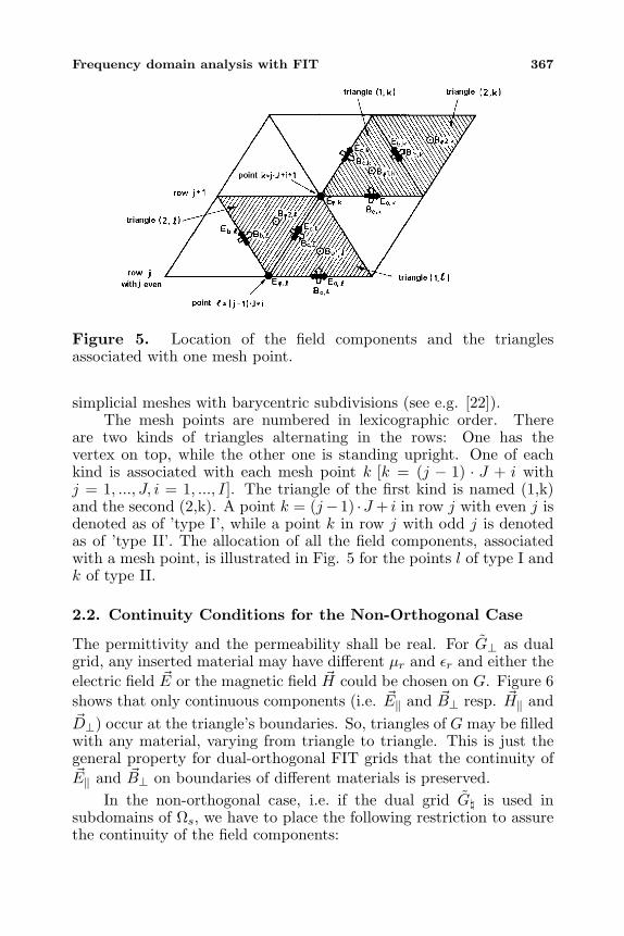
Frequency domain analysis with FIT 367
Figure 5. Location of the field components and the trianglesassociated with one mesh point.
simplicial meshes with barycentric subdivisions (see e.g. [22]).The mesh points are numbered in lexicographic order. There
are two kinds of triangles alternating in the rows: One has thevertex on top, while the other one is standing upright. One of eachkind is associated with each mesh point k [k = (j − 1) · J + i withj = 1, ..., J, i = 1, ..., I]. The triangle of the first kind is named (1,k)and the second (2,k). A point k = (j−1) ·J + i in row j with even j isdenoted as of ’type I’, while a point k in row j with odd j is denotedas of ’type II’. The allocation of all the field components, associatedwith a mesh point, is illustrated in Fig. 5 for the points l of type I andk of type II.
2.2. Continuity Conditions for the Non-Orthogonal Case
The permittivity and the permeability shall be real. For G⊥ as dualgrid, any inserted material may have different µr and εr and either theelectric field E or the magnetic field H could be chosen on G. Figure 6shows that only continuous components (i.e. E‖ and B⊥ resp. H‖ andD⊥) occur at the triangle’s boundaries. So, triangles of G may be filledwith any material, varying from triangle to triangle. This is just thegeneral property for dual-orthogonal FIT grids that the continuity ofE‖ and B⊥ on boundaries of different materials is preserved.
In the non-orthogonal case, i.e. if the dual grid G is used insubdomains of Ωs, we have to place the following restriction to assurethe continuity of the field components:
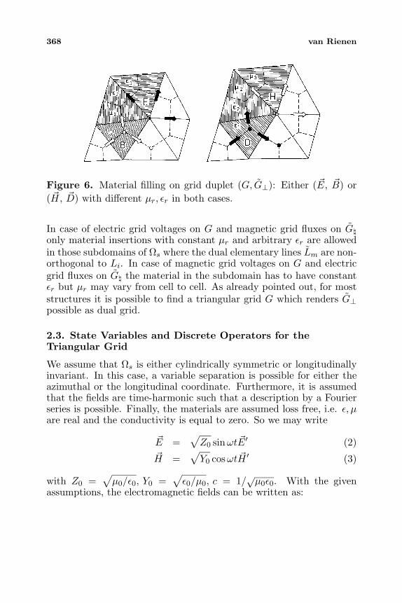
368 van Rienen
Figure 6. Material filling on grid duplet (G, G⊥): Either ( E, B) or( H, D) with different µr, εr in both cases.
In case of electric grid voltages on G and magnetic grid fluxes on G
only material insertions with constant µr and arbitrary εr are allowedin those subdomains of Ωs where the dual elementary lines Lm are non-orthogonal to Li. In case of magnetic grid voltages on G and electricgrid fluxes on G the material in the subdomain has to have constantεr but µr may vary from cell to cell. As already pointed out, for moststructures it is possible to find a triangular grid G which renders G⊥possible as dual grid.
2.3. State Variables and Discrete Operators for theTriangular Grid
We assume that Ωs is either cylindrically symmetric or longitudinallyinvariant. In this case, a variable separation is possible for either theazimuthal or the longitudinal coordinate. Furthermore, it is assumedthat the fields are time-harmonic such that a description by a Fourierseries is possible. Finally, the materials are assumed loss free, i.e. ε, µare real and the conductivity is equal to zero. So we may write
E =√
Z0 sinωt E′ (2)H =
√Y0 cosωt H ′ (3)
with Z0 =√
µ0/ε0, Y0 =√
ε0/µ0, c = 1/√
µ0ε0. With the givenassumptions, the electromagnetic fields can be written as:
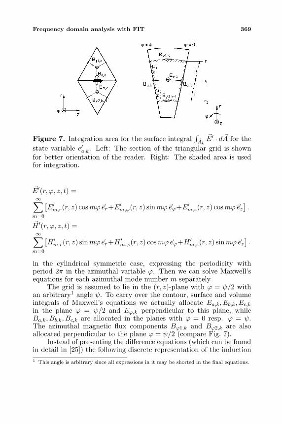
Frequency domain analysis with FIT 369
Figure 7. Integration area for the surface integral∫Ak
E′ · d A for thestate variable e′a,k. Left: The section of the triangular grid is shownfor better orientation of the reader. Right: The shaded area is usedfor integration.
E′(r, ϕ, z, t) =∞∑
m=0
[E′m,r(r, z) cosmϕer+E′m,ϕ(r, z) sinmϕeϕ+E′m,z(r, z) cosmϕez
].
H ′(r, ϕ, z, t) =∞∑
m=0
[H ′m,r(r, z) sinmϕer+H ′m,ϕ(r, z) cosmϕeϕ+H ′m,z(r, z) sinmϕez
].
in the cylindrical symmetric case, expressing the periodicity withperiod 2π in the azimuthal variable ϕ. Then we can solve Maxwell’sequations for each azimuthal mode number m separately.
The grid is assumed to lie in the (r, z)-plane with ϕ = ψ/2 withan arbitrary1 angle ψ. To carry over the contour, surface and volumeintegrals of Maxwell’s equations we actually allocate Ea,k, Eb,k, Ec,k
in the plane ϕ = ψ/2 and Eϕ,k perpendicular to this plane, whileBa,k, Bb,k, Bc,k are allocated in the planes with ϕ = 0 resp. ϕ = ψ.The azimuthal magnetic flux components Bϕ1,k and Bϕ2,k are alsoallocated perpendicular to the plane ϕ = ψ/2 (compare Fig. 7).
Instead of presenting the difference equations (which can be foundin detail in [25]) the following discrete representation of the induction1 This angle is arbitrary since all expressions in it may be shorted in the final equations.
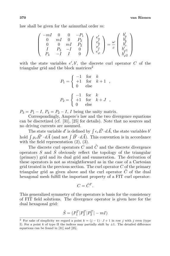
370 van Rienen
law shall be given for the azimuthal order m:−mI 0 0 −P1
0 mI 0 P2
0 0 mI P2
I P3 −I 0P4 −I I 0
e′ae′be′ce′ϕ
=
ω
c
b′ab′bb′cb′ϕ1b′ϕ2
with the state variables e′, b′, the discrete curl operator C of thetriangular grid and the block matrices2
P1 =
−1 for k+1 for k + 10 else
,
P2 =
−1 for k+1 for k + J0 else
,
P3 = P1 − I, P4 = P2 − I, I being the unity matrix.Correspondingly, Ampere’s law and the two divergence equations
can be discretized (cf. [31], [25] for details). Note that no sources andno driving currents are assumed.
The state variable d′ is defined by∫
εr E′ ·d A, the state variables b′
hold∫
µrH ′ · d A (and not
∫B′ · d A). This convention is in accordance
with the field representation (2), (3).The discrete curl operators C and C and the discrete divergence
operators S and S obviously reflect the topology of the triangular(primary) grid and its dual grid and enumeration. The derivation ofthese operators is not as straightforward as in the case of a Cartesiangrid treated in the previous section. The curl operator C of the primarytriangular grid as given above and the curl operator C of the dualhexagonal mesh fulfill the important property of a FIT curl operator:
C = CT .
This generalized symmetry of the operators is basis for the consistencyof FIT field solutions. The divergence operator is given here for thedual hexagonal grid:
S = (P T1 |P T
2 |P T2 | −mI)
2 For sake of simplicity we regard a point k = (j − 1) · J + 1 in row j with j even (typeI). For a point k of type II the indices may partially shift by ±1. The detailed differenceequations can be found in [31] and [25].
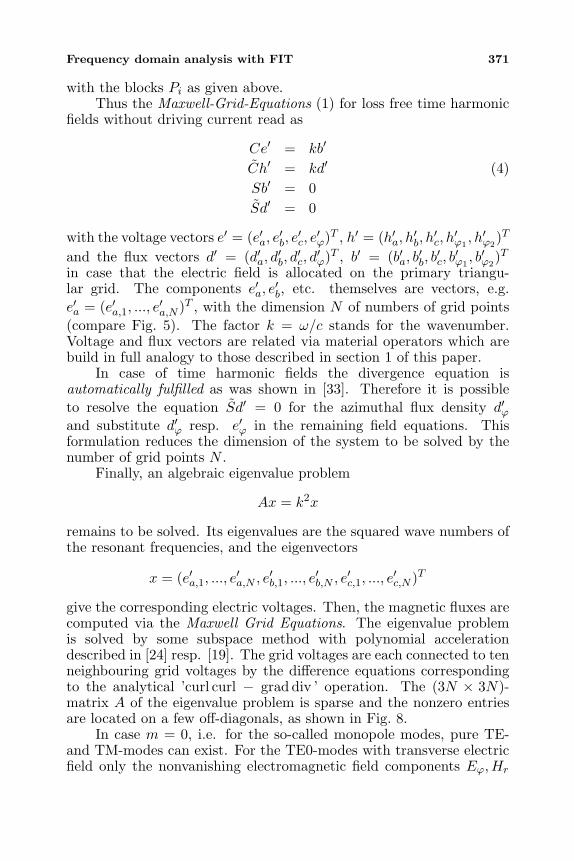
Frequency domain analysis with FIT 371
with the blocks Pi as given above.Thus the Maxwell-Grid-Equations (1) for loss free time harmonic
fields without driving current read as
Ce′ = kb′
Ch′ = kd′ (4)Sb′ = 0Sd′ = 0
with the voltage vectors e′ = (e′a, e′b, e′c, e′ϕ)T , h′ = (h′a, h
′b, h′c, h′ϕ1
, h′ϕ2)T
and the flux vectors d′ = (d′a, d′b, d′c, d′ϕ)T , b′ = (b′a, b
′b, b′c, b′ϕ1
, b′ϕ2)T
in case that the electric field is allocated on the primary triangu-lar grid. The components e′a, e
′b, etc. themselves are vectors, e.g.
e′a = (e′a,1, ..., e′a,N )T , with the dimension N of numbers of grid points
(compare Fig. 5). The factor k = ω/c stands for the wavenumber.Voltage and flux vectors are related via material operators which arebuild in full analogy to those described in section 1 of this paper.
In case of time harmonic fields the divergence equation isautomatically fulfilled as was shown in [33]. Therefore it is possibleto resolve the equation Sd′ = 0 for the azimuthal flux density d′ϕand substitute d′ϕ resp. e′ϕ in the remaining field equations. Thisformulation reduces the dimension of the system to be solved by thenumber of grid points N .
Finally, an algebraic eigenvalue problem
Ax = k2x
remains to be solved. Its eigenvalues are the squared wave numbers ofthe resonant frequencies, and the eigenvectors
x = (e′a,1, ..., e′a,N , e′b,1, ..., e
′b,N , e′c,1, ..., e
′c,N )T
give the corresponding electric voltages. Then, the magnetic fluxes arecomputed via the Maxwell Grid Equations. The eigenvalue problemis solved by some subspace method with polynomial accelerationdescribed in [24] resp. [19]. The grid voltages are each connected to tenneighbouring grid voltages by the difference equations correspondingto the analytical ’curl curl − grad div ’ operation. The (3N × 3N)-matrix A of the eigenvalue problem is sparse and the nonzero entriesare located on a few off-diagonals, as shown in Fig. 8.
In case m = 0, i.e. for the so-called monopole modes, pure TE-and TM-modes can exist. For the TE0-modes with transverse electricfield only the nonvanishing electromagnetic field components Eϕ, Hr
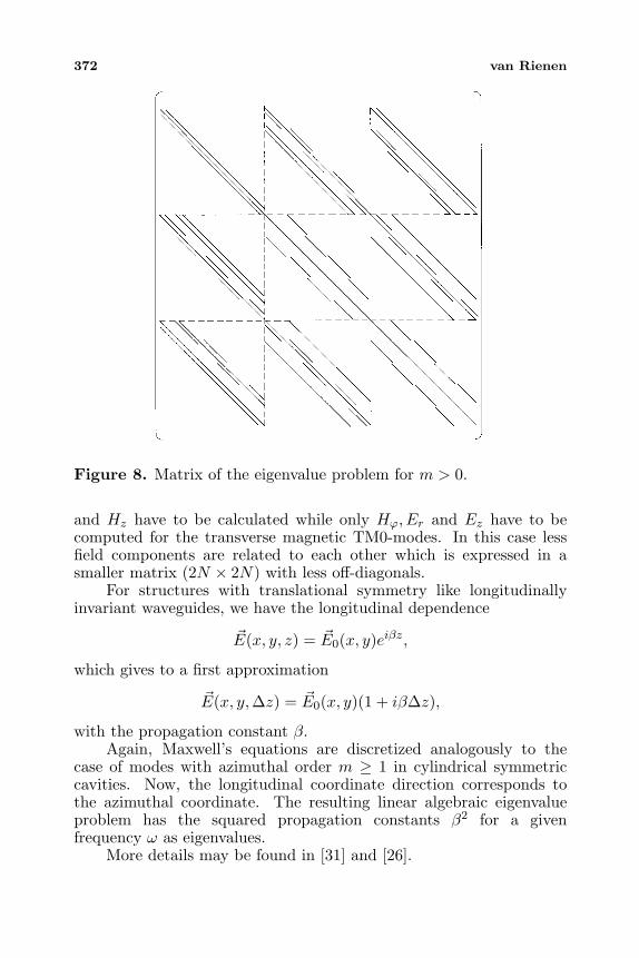
372 van Rienen
Figure 8. Matrix of the eigenvalue problem for m > 0.
and Hz have to be calculated while only Hϕ, Er and Ez have to becomputed for the transverse magnetic TM0-modes. In this case lessfield components are related to each other which is expressed in asmaller matrix (2N × 2N) with less off-diagonals.
For structures with translational symmetry like longitudinallyinvariant waveguides, we have the longitudinal dependence
E(x, y, z) = E0(x, y)eiβz,
which gives to a first approximation
E(x, y,∆z) = E0(x, y)(1 + iβ∆z),
with the propagation constant β.Again, Maxwell’s equations are discretized analogously to the
case of modes with azimuthal order m ≥ 1 in cylindrical symmetriccavities. Now, the longitudinal coordinate direction corresponds tothe azimuthal coordinate. The resulting linear algebraic eigenvalueproblem has the squared propagation constants β2 for a givenfrequency ω as eigenvalues.
More details may be found in [31] and [26].
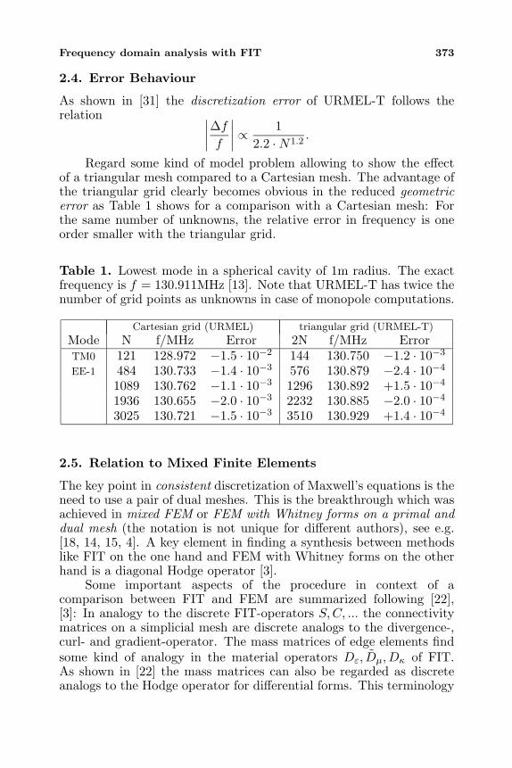
Frequency domain analysis with FIT 373
2.4. Error Behaviour
As shown in [31] the discretization error of URMEL-T follows therelation ∣∣∣∣∆f
f
∣∣∣∣ ∝ 12.2 ·N1.2
.
Regard some kind of model problem allowing to show the effectof a triangular mesh compared to a Cartesian mesh. The advantage ofthe triangular grid clearly becomes obvious in the reduced geometricerror as Table 1 shows for a comparison with a Cartesian mesh: Forthe same number of unknowns, the relative error in frequency is oneorder smaller with the triangular grid.
Table 1. Lowest mode in a spherical cavity of 1m radius. The exactfrequency is f = 130.911MHz [13]. Note that URMEL-T has twice thenumber of grid points as unknowns in case of monopole computations.
Cartesian grid (URMEL) triangular grid (URMEL-T)
Mode N f/MHz Error 2N f/MHz ErrorTM0 121 128.972 −1.5 · 10−2 144 130.750 −1.2 · 10−3
EE-1 484 130.733 −1.4 · 10−3 576 130.879 −2.4 · 10−4
1089 130.762 −1.1 · 10−3 1296 130.892 +1.5 · 10−4
1936 130.655 −2.0 · 10−3 2232 130.885 −2.0 · 10−4
3025 130.721 −1.5 · 10−3 3510 130.929 +1.4 · 10−4
2.5. Relation to Mixed Finite Elements
The key point in consistent discretization of Maxwell’s equations is theneed to use a pair of dual meshes. This is the breakthrough which wasachieved in mixed FEM or FEM with Whitney forms on a primal anddual mesh (the notation is not unique for different authors), see e.g.[18, 14, 15, 4]. A key element in finding a synthesis between methodslike FIT on the one hand and FEM with Whitney forms on the otherhand is a diagonal Hodge operator [3].
Some important aspects of the procedure in context of acomparison between FIT and FEM are summarized following [22],[3]: In analogy to the discrete FIT-operators S,C, ... the connectivitymatrices on a simplicial mesh are discrete analogs to the divergence-,curl- and gradient-operator. The mass matrices of edge elements findsome kind of analogy in the material operators Dε, Dµ, Dκ of FIT.As shown in [22] the mass matrices can also be regarded as discreteanalogs to the Hodge operator for differential forms. This terminology
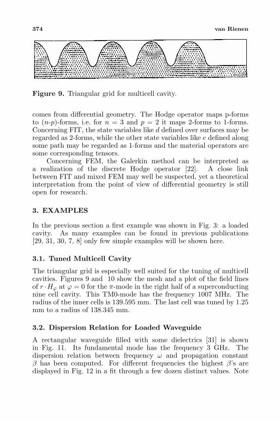
374 van Rienen
Figure 9. Triangular grid for multicell cavity.
comes from differential geometry. The Hodge operator maps p-formsto (n-p)-forms, i.e. for n = 3 and p = 2 it maps 2-forms to 1-forms.Concerning FIT, the state variables like d defined over surfaces may beregarded as 2-forms, while the other state variables like e defined alongsome path may be regarded as 1-forms and the material operators aresome corresponding tensors.
Concerning FEM, the Galerkin method can be interpreted asa realization of the discrete Hodge operator [22]. A close linkbetween FIT and mixed FEM may well be suspected, yet a theoreticalinterpretation from the point of view of differential geometry is stillopen for research.
3. EXAMPLES
In the previous section a first example was shown in Fig. 3: a loadedcavity. As many examples can be found in previous publications[29, 31, 30, 7, 8] only few simple examples will be shown here.
3.1. Tuned Multicell Cavity
The triangular grid is especially well suited for the tuning of multicellcavities. Figures 9 and 10 show the mesh and a plot of the field linesof r ·Hϕ at ϕ = 0 for the π-mode in the right half of a superconductingnine cell cavity. This TM0-mode has the frequency 1007 MHz. Theradius of the inner cells is 139.595 mm. The last cell was tuned by 1.25mm to a radius of 138.345 mm.
3.2. Dispersion Relation for Loaded Waveguide
A rectangular waveguide filled with some dielectrics [31] is shownin Fig. 11. Its fundamental mode has the frequency 3 GHz. Thedispersion relation between frequency ω and propagation constantβ has been computed. For different frequencies the highest β’s aredisplayed in Fig. 12 in a fit through a few dozen distinct values. Note
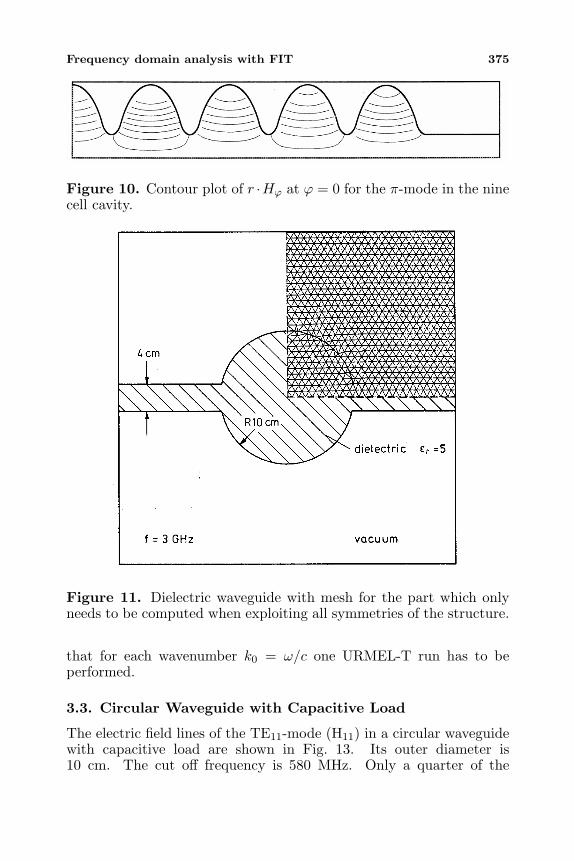
Frequency domain analysis with FIT 375
Figure 10. Contour plot of r ·Hϕ at ϕ = 0 for the π-mode in the ninecell cavity.
Figure 11. Dielectric waveguide with mesh for the part which onlyneeds to be computed when exploiting all symmetries of the structure.
that for each wavenumber k0 = ω/c one URMEL-T run has to beperformed.
3.3. Circular Waveguide with Capacitive Load
The electric field lines of the TE11-mode (H11) in a circular waveguidewith capacitive load are shown in Fig. 13. Its outer diameter is10 cm. The cut off frequency is 580 MHz. Only a quarter of the
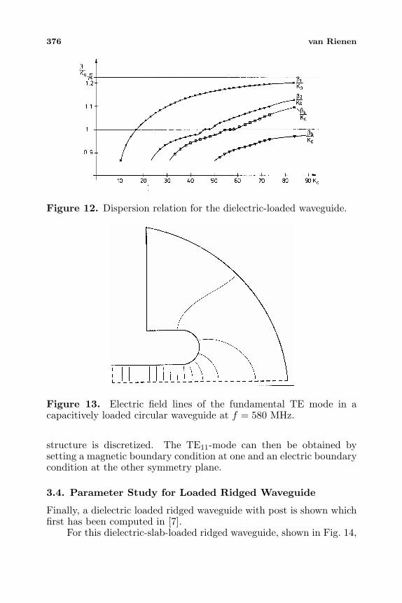
376 van Rienen
Figure 12. Dispersion relation for the dielectric-loaded waveguide.
Figure 13. Electric field lines of the fundamental TE mode in acapacitively loaded circular waveguide at f = 580 MHz.
structure is discretized. The TE11-mode can then be obtained bysetting a magnetic boundary condition at one and an electric boundarycondition at the other symmetry plane.
3.4. Parameter Study for Loaded Ridged Waveguide
Finally, a dielectric loaded ridged waveguide with post is shown whichfirst has been computed in [7].
For this dielectric-slab-loaded ridged waveguide, shown in Fig. 14,
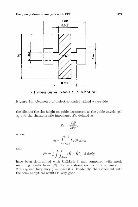
Frequency domain analysis with FIT 377
Figure 14. Geometry of dielectric-loaded ridged waveguide.
the effect of the slot height on guide parameters as the guide wavelengthλg and the characteristic impedance Z0, defined as
Z0 =|V0|22PT
,
where
V0 =∫ b1/2
−b1/2Ey(0, y)dy
andPT =
12
∫ ∫Area
( E × H∗) · z dxdy,
have been determined with URMEL–T and compared with modematching results from [32]. Table 2 shows results for the case εr =2.62 · ε0 and frequency f = 5.95 GHz. Evidently, the agreement withthe semi-analytical results is very good.
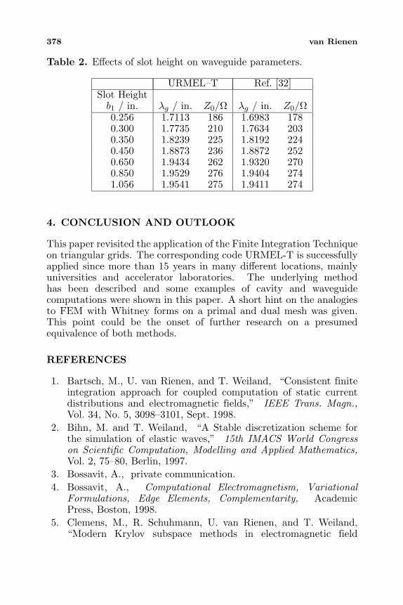
378 van Rienen
Table 2. Effects of slot height on waveguide parameters.
URMEL–T Ref. [32]Slot Height
b1 / in. λg / in. Z0/Ω λg / in. Z0/Ω0.256 1.7113 186 1.6983 1780.300 1.7735 210 1.7634 2030.350 1.8239 225 1.8192 2240.450 1.8873 236 1.8872 2520.650 1.9434 262 1.9320 2700.850 1.9529 276 1.9404 2741.056 1.9541 275 1.9411 274
4. CONCLUSION AND OUTLOOK
This paper revisited the application of the Finite Integration Techniqueon triangular grids. The corresponding code URMEL-T is successfullyapplied since more than 15 years in many different locations, mainlyuniversities and accelerator laboratories. The underlying methodhas been described and some examples of cavity and waveguidecomputations were shown in this paper. A short hint on the analogiesto FEM with Whitney forms on a primal and dual mesh was given.This point could be the onset of further research on a presumedequivalence of both methods.
REFERENCES
1. Bartsch, M., U. van Rienen, and T. Weiland, “Consistent finiteintegration approach for coupled computation of static currentdistributions and electromagnetic fields,” IEEE Trans. Magn.,Vol. 34, No. 5, 3098–3101, Sept. 1998.
2. Bihn, M. and T. Weiland, “A Stable discretization scheme forthe simulation of elastic waves,” 15th IMACS World Congresson Scientific Computation, Modelling and Applied Mathematics,Vol. 2, 75–80, Berlin, 1997.
3. Bossavit, A., private communication.4. Bossavit, A., Computational Electromagnetism, Variational
Formulations, Edge Elements, Complementarity, AcademicPress, Boston, 1998.
5. Clemens, M., R. Schuhmann, U. van Rienen, and T. Weiland,“Modern Krylov subspace methods in electromagnetic field
Frequency domain analysis with FIT 379
computation using the finite integration theory,” ACES Journal,Special Issue on Applied Mathematics: Meeting the ChallengesPresented by Computational Electromagnetics, Vol. 11, No. 1, 70–84, March 1996.
6. Clemens, M., P. Thoma, T. Weiland, and U. van Rienen, “Asurvey on the computational electromagnetic field calculation withthe FI method,” Surveys on Mathematics for Industry, Vol. 8,No. 3–4, 213–232, 1999.
7. Cooper, R. K., M. J. Browman, T. Weiland, and U. van Rienen,“Waveguide calculations using established codes,” IEEE Trans.Electron Devices, Vol. 35, No. 11, 2044–2047, 1988.
8. Cooper, R. K., U. van Rienen, and T. Weiland, “RF waveguidedesign by proven electromagnetic CAD systems,” GeneralAssembly of the URSI, Israel, Tel Aviv, August 1987.
9. Dehler, M., “Numerische losung der Maxwellschen Gleichungenauf kreiszylindrischen gittern,” Ph.D. thesis, Darmstadt Univer-sity of Technology, 1993.
10. Dehler, M. and T. Weiland, “A new spectral domain technique forthe calculation of eigenvalues in curvilinear coordinates,” IEEETrans. Magn., Vol. 30, No. 5, 3574–3577, 1994.
11. Dohlus, M., P. Thoma, and T. Weiland, “Stability offinite difference time domain methods related to space andtime discretization,” IEEE Trans. Microwave Theory Tech.,submitted.
12. Fellinger, P., “Ein Verfahren zur numerischen losung elastis-cher wellenausbreitungsprobleme im zeitbereich durch direktediskretisierung der elastodynamischen grundgleichungen,” Ph.D.thesis, Gesamthochschule Kassel, 1991.
13. Henke, H., Spherical Modes, ISR-RF 81-29, CERN, Geneva,Switzerland, 1981.
14. Nedelec, J., “Mixed finite elements in R3,” Numer. Math., Vol. 35,315–341, 1980.
15. Nedelec, J., “A new family of mixed finite elements in R3,”Numer. Math., Vol. 50, 57–81, 1986.
16. Pinder, P., “Zur numerischen berechnung gekoppelter elektro-magnetischer und thermischer felder,” Ph.D. thesis, DarmstadtUniversity of Technology, 1998.
17. Pinder, P. and T. Weiland, “Numerical calculation of coupledelectromagnetic and thermal fields using the finite integrationmethod,” PIERS’96, 1996.
18. Raviart, P.-A. and J.-M. Thomas, “A mixed finite element
380 van Rienen
method for second order elliptic problems,” Mathematical Aspectsof the Finite Element Method, I. Galligani and E. Magenes (eds.),292–315. Springer-Verlag, 1977.
19. Schmitt, D. and T. Weiland, “2D and 3D computations ofeigenvalue problems,” IEEE Trans. Microwave Theory Tech., Vol.28, No. 2, 1793–1796, 1992.
20. Schuhmann, R. and T. Weiland, “Stability of FDTD algorithm onnonorthogonal grids related to the spatial interpolation scheme,”IEEE Trans. Microwave Theory Tech., Vol. 34, No. 5, 2751–2754,Sept. 1998.
21. Schuhmann, R. and T. Weiland, “A stable interpolation techniquefor FDTD on nonorthogonal grids,” Int. J. Numerical Modelling,Focused Issue on “Finite Difference Time and Frequency DomainMethods”, Vol. 11, 299–306, 1998.
22. Tarhasaari, T., L. Kettunen, and A. Bossavit, “An interpretationof the Galerkin method as the realization of a discrete hodgeoperator,” 8th Biennal IEEE Conf. on Electromagnetic FieldComputation CEFC 1998, Tucson, Arizona, USA, June 1998.
23. Thoma, P. and T. Weiland, “A consistent subgridding schemefor the finite difference time domain method,” Int. J. NumericalModelling, Vol. 9, 359–374, 1996.
24. Tuckmantel, J., Application of SAP in URMEL, EF/RF 85-4,CERN, Geneva, Switzerland, July 1985.
25. van Rienen, U., “Zur numerischen Berechnung zeitharmonischerelektromagnetischer felder in offenen, zylindersymmetrischenstrukturen unter verwendung von mehrgitterverfahren,” Ph.D.thesis, Darmstadt University of Technology, 1989.
26. van Rienen, U., “Finite integration technique on triangular gridsrevisited,” Int. J. Numerical Modelling: Electronic Networks,Devices and Fields, Special Issue “Finite Difference Time andFrequency Domain Methods”, Vol. 12, 107–128, 1999.
27. van Rienen, U., Numerical Methods in Computational Electrody-namics - Linear Systems in Practical Applications, Vol. 12 of Lec-ture Notes in Computational Science and Engineering, Springer,2000.
28. van Rienen, U., P. Pinder, and T. Weiland, “Consistentfinite integration approach for the coupled calculation ofelectromagnetic fields and stationary temperature distributions,”In 7th Biennal IEEE Conference on Electromagnetic FieldComputation (CEFC), 294, Okayama, Japan, March 1996.
29. van Rienen, U. and T. Weiland, “Triangular discretization
Frequency domain analysis with FIT 381
method for the evaluation of RF-fields in cylindrically symmetriccavities,” IEEE Trans. Magn., Vol. 21, No. 6, 2317–2320,November 1985.
30. van Rienen, U. and T. Weiland, “Cavity and waveguide design bytriangular mesh code URMEL-T,” Int. Linear Accelerator Conf.LINAC’86, No. SLAC-303, 286, Stanford University, June 1986.
31. van Rienen, U. and T. Weiland, “Triangular discretizationmethod for the evaluation of RF-fields in waveguides andcylindrically symmetric cavities,” Part. Acc., Vol. 20, 239–267,1986/87.
32. Villeneuve, A. T., “Analysis of slotted, dielectrically loaded,rigded waveguide,” IEEE Trans. Microwave Theory Tech.,Vol. 32, 524–532, 1984.
33. Weiland, T., “Eine methode zur losung der MaxwellschenGleichungen fur sechskomponentige felder auf diskreter basis,”Archiv fur Elektrotechnik, Vol. 31, 116–120, 1977.
34. Weiland, T., “Zur berechnung der wirbelstrome in beliebiggeformten, lamellierten, dreidimensionalen eisenkorpern,” Archivfur Elektrotechnik, Vol. 60, 345–351, 1978.
35. Weiland, T., “On the unique numerical solution of MaxwellianEigenvalue problems in three dimensions,” Part. Acc., Vol. 17,227–242, 1985.
36. Weiland, T., “Ein allgemeines verfahren zur losung derMaxwell’schen Gleichungen und seine anwendung in physik undtechnik,” Physikalische Blatter, Vol. 41, 380, 1986.
37. Weiland, T., “Elektromagnetisches CAD — rechnergestutztemethoden zur berechnung von feldern,” Script, DarmstadtUniversity of Technology, May 1995.
38. Weiland, T., “High precision eigenmode computation,” Part.Acc., Vol. 56, 61–82, 1996.
39. Wolter, H., “Berechnung akustischer wellen und resonatorenmit der FIT-methode,” Ph.D. thesis, Darmstadt University ofTechnology, 1995.
40. Yee, K. S., “Numerical solution of initial boundary value problemsinvolving Maxwell’s equations in isotropic media,” IEEE Trans.Antennas Propagat., Vol. 14, 302–307, 1966.
Progress In Electromagnetics Research, PIER 32, 383–411, 2001
IMPLEMENTING THE PERFECTLY MATCHED LAYERABSORBING BOUNDARY CONDITION WITHMIMETIC DIFFERENCING SCHEMES
M. W. Buksas
Los Alamos National Laboratory, MS B-258Los Alamos, New Mexico 87545, USA
Abstract—This paper concerns the implementation of the perfectlymatched layer (PML) absorbing boundary condition in the frameworkof a mimetic differencing scheme for Maxwell’s Equations.
We use mimetic versions of the discrete curl operator on irregularlogically rectangular grids to implement anisotropic tensor formulationof the PML. The form of the tensor we use is fixed with respect to thegrid and is known to be perfectly matched in the continuous limitfor orthogonal coordinate systems in which the metric is constant,i.e. Cartesian coordinates, and quasi-perfectly matched (quasi-PML)for curvilinear coordinates. Examples illustrating the effectivenessand long-term stability of the methods are presented. Theseexamples demonstrate that the grid-based coordinate implementationof the PML is effective on Cartesian grids, but generates systematicreflections on grids which are orthogonal but non-Cartesian (quasi-PML). On non-orthogonal grids progressively worse performance ofthe PML is demonstrated.
The paper begins with a summary derivation of the anisotropicformulation of the perfectly matched layer and mimetic differencingschemes for irregular logically rectangular grids.
1 Background1.1 The PML Absorbing Boundary Condition1.2 Expressing the PML on General Grids1.3 Background on Mimetic Difference Schemes1.4 Application of Mimetic Difference Operators to
Maxwell’s Equations
384 Buksas
2 Implementation2.1 Combining the PML Equations and Mimetic Difference
Operators2.2 Conversion to the Time Domain2.3 Discretization of the Equations
3 Test Problems and Results3.1 Radiation Problem on a Cartesian Grid3.2 Scattering Problem on a Polar Grid3.3 Skew Grid
4 Conclusions
Acknowledgment
References
1. BACKGROUND
1.1. The PML Absorbing Boundary Condition
The need for absorbing boundary conditions arises when we wish tosimulate problems which are naturally cast on unbounded domains.Hyperbolic problems in which features of the solution move at finitespeed are limited in duration by the return of outwardly propagatingfeatures of the solution after interacting with the boundaries of thecomputational domain. This situation is illustrated graphically inFigure 1. Here the domain of interest is surrounded by a buffer layerwhose purpose is to delay the return of the reflection. To increase theduration of validity, we must increase the size of the boundary region,with a corresponding increase in computational cost.
The perfectly matched layer and other absorbing domain methodsmodify the equations in the buffer region to damp the waves as theytravel through it. The goal is to attenuate these waves to a level wherethey can be ignored when they return to the domain of interest. Thecomputational advantages of the PML over other absorbing boundaryconditions include its applicability to various numerical methods andit relative ease of implementation.
In [2], Berenger considered the problem of attaining perfecttransmission of planar electromagnetic waves across a planar interfacebetween empty space and a material half-space. This is accomplishedby adding additional degrees of freedom to Maxwell’s equationsthrough a field splitting, where a single field is split into the sum oftwo parts which evolve according to separate equations. Subsequent
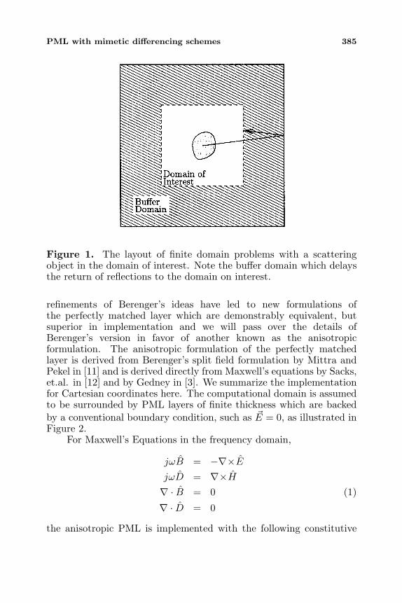
PML with mimetic differencing schemes 385
Figure 1. The layout of finite domain problems with a scatteringobject in the domain of interest. Note the buffer domain which delaysthe return of reflections to the domain on interest.
refinements of Berenger’s ideas have led to new formulations ofthe perfectly matched layer which are demonstrably equivalent, butsuperior in implementation and we will pass over the details ofBerenger’s version in favor of another known as the anisotropicformulation. The anisotropic formulation of the perfectly matchedlayer is derived from Berenger’s split field formulation by Mittra andPekel in [11] and is derived directly from Maxwell’s equations by Sacks,et.al. in [12] and by Gedney in [3]. We summarize the implementationfor Cartesian coordinates here. The computational domain is assumedto be surrounded by PML layers of finite thickness which are backedby a conventional boundary condition, such as E = 0, as illustrated inFigure 2.
For Maxwell’s Equations in the frequency domain,
jωB = −∇×E
jωD = ∇×H
∇ · B = 0 (1)
∇ · D = 0
the anisotropic PML is implemented with the following constitutive
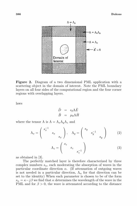
386 Buksas
Figure 2. Diagram of a two dimensional PML application with ascattering object in the domain of interest. Note the PML boundarylayers on all four sides of the computational region and the four cornerregions with overlapping layers.
laws
D = ε0ΛE
B = µ0ΛH
where the tensor Λ is Λ = ΛxΛyΛz and
Λx =
s−1
xsx
sx
, Λy =
sy
s−1y
sy
(2)
Λz =
sz
szs−1z
(3)
as obtained in [3].The perfectly matched layer is therefore characterized by three
complex numbers sα, each moderating the absorption of waves in theparticular coordinate direction α. (If attenuation of outgoing wavesis not needed in a particular direction, Λα for that direction can beset to the identity) When each parameter is chosen to be of the formsα = κ−jβ we find that κ determines the wavelength of the wave in thePML and for β > 0, the wave is attenuated according to the distance
PML with mimetic differencing schemes 387
of travel in the α direction. For the interior computational domain, theconstitutive laws reduce to that of free space when sx = sy = sz = 1.
This result generalized in the obvious way for boundary layerswhich are matched to regions other than free space, regardless of thefrequency-dependence of these parameters, (as noted in [13, p.323]),allowing us to write the general constitutive laws for perfectly matchedlayers which match dispersive media:
D = ε(ω)ΛE
B = µ(ω)ΛH
This is also demonstrated in the context of a different derivation ofthe PML for both dispersive and anisotropic media in [15]. For ourpurposes, we will focus on the problem of matching PMLs to non-dispersive dielectrics. For these problems, the complete system ofMaxwell’s equations is:
jωB = −∇×E
jωD = ∇×H (4)
D = εΛE
B = µΛH
When designing PMLs for time domain simulations theparameters sα should be chosen so that the resulting frequency domainequations can be easily converted back into the time domain. Thesimplest of these is sα = 1 + σα/ε0jω which we employ here. Moregenerally, the expression sα = κα + σα/ε0jω has been used in [4] aswell as sα = 1 + σα/(1 + βjω) in [17]. More general constitutivelaws, such as the biaxial formulation in [18] have also been successfullyemployed.
Although the mimetic differencing schemes discussed in the nextsection are capable of handling discontinuous coefficients, we do notcurrently cast the PML equations in a form which will allow it to doso. (This may be responsible for persistent reflections which are visiblein some test problems.) This difficulty arises from the frequency-dependent nature of the operator Λ and is shared by other problemswith frequency dependent parameters, including ordinary dispersivematerials. To reduce numerical reflections caused by discontinuouscoefficients in the PML, the σα (and other parameters if present)are chosen to be functions of the coordinate variable α. Choosingthese functions so that sα = 1 at the interface makes the PMLa continuous extension of the medium being matched and reducesnumerical reflections at the interface. Increasing the value of σ (and
388 Buksas
possibly other coefficients) with depth in the layer allows for greateroverall attenuation while keeping down the numerical reflections causedby the varying parameter. Gedney [3] suggests a conductivity profile
σ(z) =σmax|z − z0|m
dm(5)
where d is the depth of the layer, z0 is the interface and m is the chosenpower of variation. Values of m between 3 and 4 are believed to beoptimal.
1.2. Expressing the PML on General Grids
The mimetic differencing scheme we will describe in Section 1.3 iscapable of handling non-Cartesian two-dimensional grids. To takeadvantage of this flexibility, we consider the problem of expressingthe PML equations in terms of an underlying grid, without referenceto a particular coordinate scheme. Since we are interested in twodimensional problems, we assume homogeneity of both the problemand the underlying grid in the z direction. We will refer to the othertwo coordinate variables as (ξ, η) and the entire set of coordinates as(ξ, η, z).
Since the grids we wish to apply this technique to are not theresult of a known transformation of the general coordinates (ξ, η) intothe Cartesian coordinates (x, y). The logically rectangular nature ofthe grid, however, makes if possible to assign integer (ξ, η) coordinatesto the nodal points and, by interpolation, to assign (ξ, η) coordinatesto all points in the grid. (Generally, only the integer and integer-plus-half coordinates are used, since these give the nodes, edge centersand cell centers.) This gives an effective inverse of the coordinatetransformation from the logical variables (ξ, η) to Cartesian variables.We note that when measured in these general coordinates, the lengthof a cell edge is always one and the width of a PML is equal to thenumber of cells that it covers.
We will assume that the coordinate scheme induced by the grid isorthogonal, hence we will retain the diagonal form of the PML tensor Λ.Furthermore, we assume that in the corner regions, the PML tensorfactors as before into components that represent attenuation in thedifferent coordinates, Λξ = diags−1
ξ , sξ, sξ, Λη = diagsη, s−1η , sη,
and Λz = diagsz, sz, s−1z . Since we are interested in two dimensional
problems in the ξ and η variables, there are no waves propagating inthe z direction and we take sz = 1. Hence, Λz is the identity matrixand will be dropped from further calculations.
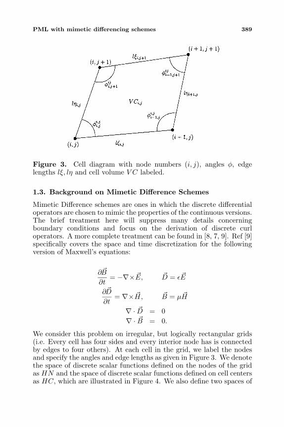
PML with mimetic differencing schemes 389
Figure 3. Cell diagram with node numbers (i, j), angles φ, edgelengths lξ, lη and cell volume V C labeled.
1.3. Background on Mimetic Difference Schemes
Mimetic Difference schemes are ones in which the discrete differentialoperators are chosen to mimic the properties of the continuous versions.The brief treatment here will suppress many details concerningboundary conditions and focus on the derivation of discrete curloperators. A more complete treatment can be found in [8, 7, 9]. Ref [9]specifically covers the space and time discretization for the followingversion of Maxwell’s equations:
∂B
∂t= −∇× E, D = ε E
∂D
∂t= ∇× H, B = µ H
∇ · D = 0∇ · B = 0.
We consider this problem on irregular, but logically rectangular grids(i.e. Every cell has four sides and every interior node has is connectedby edges to four others). At each cell in the grid, we label the nodesand specify the angles and edge lengths as given in Figure 3. We denotethe space of discrete scalar functions defined on the nodes of the gridas HN and the space of discrete scalar functions defined on cell centersas HC, which are illustrated in Figure 4. We also define two spaces of
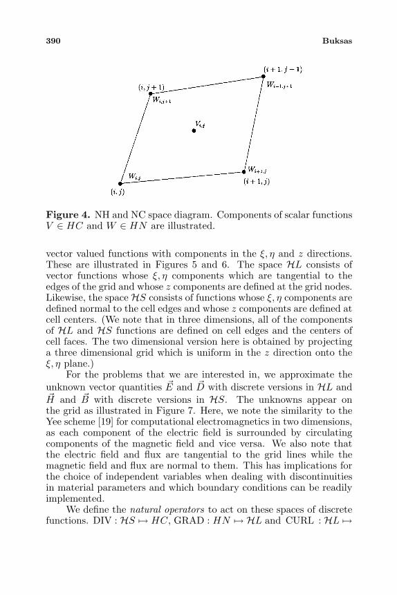
390 Buksas
Figure 4. NH and NC space diagram. Components of scalar functionsV ∈ HC and W ∈ HN are illustrated.
vector valued functions with components in the ξ, η and z directions.These are illustrated in Figures 5 and 6. The space HL consists ofvector functions whose ξ, η components which are tangential to theedges of the grid and whose z components are defined at the grid nodes.Likewise, the space HS consists of functions whose ξ, η components aredefined normal to the cell edges and whose z components are defined atcell centers. (We note that in three dimensions, all of the componentsof HL and HS functions are defined on cell edges and the centers ofcell faces. The two dimensional version here is obtained by projectinga three dimensional grid which is uniform in the z direction onto theξ, η plane.)
For the problems that we are interested in, we approximate theunknown vector quantities E and D with discrete versions in HL andH and B with discrete versions in HS. The unknowns appear onthe grid as illustrated in Figure 7. Here, we note the similarity to theYee scheme [19] for computational electromagnetics in two dimensions,as each component of the electric field is surrounded by circulatingcomponents of the magnetic field and vice versa. We also note thatthe electric field and flux are tangential to the grid lines while themagnetic field and flux are normal to them. This has implications forthe choice of independent variables when dealing with discontinuitiesin material parameters and which boundary conditions can be readilyimplemented.
We define the natural operators to act on these spaces of discretefunctions. DIV : HS → HC, GRAD : HN → HL and CURL : HL →
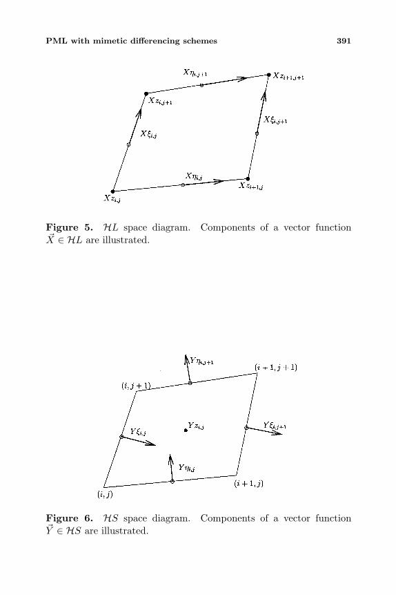
PML with mimetic differencing schemes 391
Figure 5. HL space diagram. Components of a vector functionX ∈ HL are illustrated.
Figure 6. HS space diagram. Components of a vector functionY ∈ HS are illustrated.
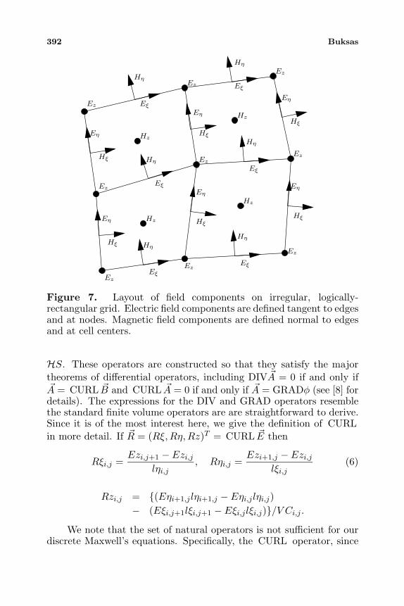
392 Buksas
EξEξ
Eξ
Eξ
Eξ
EηEη
Eη
Eη
Eη
Eη
HξHξ
Hξ
Hξ
Hξ
Hξ
HηHη
Hη
Hη
Hη
Ez
Ez
Ez
Ez
EzEz
Ez
Ez
Ez
Hz
Hz
Hη
Hz
Eξ
Hz
Figure 7. Layout of field components on irregular, logically-rectangular grid. Electric field components are defined tangent to edgesand at nodes. Magnetic field components are defined normal to edgesand at cell centers.
HS. These operators are constructed so that they satisfy the majortheorems of differential operators, including DIV A = 0 if and only ifA = CURL B and CURL A = 0 if and only if A = GRADφ (see [8] fordetails). The expressions for the DIV and GRAD operators resemblethe standard finite volume operators are are straightforward to derive.Since it is of the most interest here, we give the definition of CURLin more detail. If R = (Rξ, Rη, Rz)T = CURL E then
Rξi,j =Ezi,j+1 − Ezi,j
lηi,j, Rηi,j =
Ezi+1,j − Ezi,jlξi,j
(6)
Rzi,j = (Eηi+1,jlηi+1,j − Eηi,jlηi,j)− (Eξi,j+1lξi,j+1 − Eξi,jlξi,j)/V Ci,j .
We note that the set of natural operators is not sufficient for ourdiscrete Maxwell’s equations. Specifically, the CURL operator, since
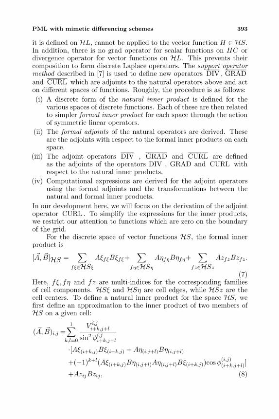
PML with mimetic differencing schemes 393
it is defined on HL, cannot be applied to the vector function H ∈ HS.In addition, there is no grad operator for scalar functions on HC ordivergence operator for vector functions on HL. This prevents theircomposition to form discrete Laplace operators. The support operatormethod described in [7] is used to define new operators DIV , GRADand CURL which are adjoints to the natural operators above and acton different spaces of functions. Roughly, the procedure is as follows:(i) A discrete form of the natural inner product is defined for the
various spaces of discrete functions. Each of these are then relatedto simpler formal inner product for each space through the actionof symmetric linear operators.
(ii) The formal adjoints of the natural operators are derived. Theseare the adjoints with respect to the formal inner products on eachspace.
(iii) The adjoint operators DIV , GRAD and CURL are definedas the adjoints of the operators DIV , GRAD and CURL withrespect to the natural inner products.
(iv) Computational expressions are derived for the adjoint operatorsusing the formal adjoints and the transformations between thenatural and formal inner products.
In our development here, we will focus on the derivation of the adjointoperator CURL . To simplify the expressions for the inner products,we restrict our attention to functions which are zero on the boundaryof the grid.
For the discrete space of vector functions HS, the formal innerproduct is
[ A, B]HS =∑
fξ∈HSξ
AξfξBξfξ+∑
fη∈HSη
AηfηBηfη+∑
fz∈HSz
AzfzBzfz.
(7)Here, fξ, fη and fz are multi-indices for the corresponding familiesof cell components. HSξ and HSη are cell edges, while HSz are thecell centers. To define a natural inner product for the space HS, wefirst define an approximation to the inner product of two members ofHS on a given cell:
( A, B)i,j =1∑
k,l=0
V i,ji+k,j+l
sin2 φi,ji+k,j+l
·[Aξ(i+k,j)Bξ(i+k,j) + Aη(i,j+l)Bη(i,j+l)
+(−1)k+l(Aξ(i+k,j)Bη(i,j+l)Aη(i,j+l)Bξ(i+k,j))cos φ(i,j)(i+k,j+l)]
+AzijBzij , (8)
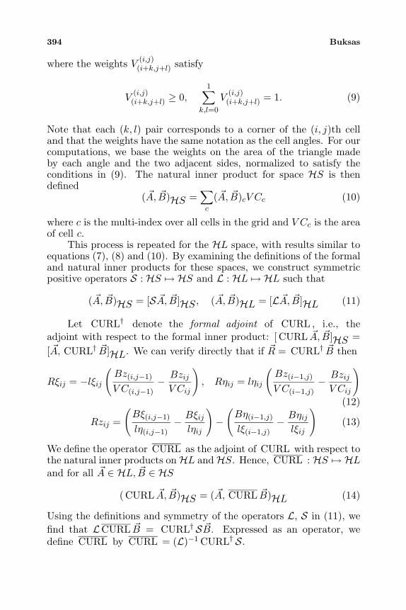
394 Buksas
where the weights V(i,j)(i+k,j+l) satisfy
V(i,j)(i+k,j+l) ≥ 0,
1∑k,l=0
V(i,j)(i+k,j+l) = 1. (9)
Note that each (k, l) pair corresponds to a corner of the (i, j)th celland that the weights have the same notation as the cell angles. For ourcomputations, we base the weights on the area of the triangle madeby each angle and the two adjacent sides, normalized to satisfy theconditions in (9). The natural inner product for space HS is thendefined
( A, B)HS =∑c
( A, B)cV Cc (10)
where c is the multi-index over all cells in the grid and V Cc is the areaof cell c.
This process is repeated for the HL space, with results similar toequations (7), (8) and (10). By examining the definitions of the formaland natural inner products for these spaces, we construct symmetricpositive operators S : HS → HS and L : HL → HL such that
( A, B)HS = [S A, B]HS, ( A, B)HL = [L A, B]HL (11)
Let CURL† denote the formal adjoint of CURL , i.e., theadjoint with respect to the formal inner product: [ CURL A, B]HS =[ A, CURL† B]HL. We can verify directly that if R = CURL† B then
Rξij = −lξij
(Bz(i,j−1)
V C(i,j−1)− Bzij
V Cij
), Rηij = lηij
(Bz(i−1,j)
V C(i−1,j)− Bzij
V Cij
)
(12)
Rzij =
(Bξ(i,j−1)
lη(i,j−1)− Bξij
lηij
)−
(Bη(i−1,j)
lξ(i−1,j)− Bηij
lξij
)(13)
We define the operator CURL as the adjoint of CURL with respect tothe natural inner products onHL andHS. Hence, CURL : HS → HL
and for all A ∈ HL, B ∈ HS
( CURL A, B)HS = ( A, CURL B)HL (14)
Using the definitions and symmetry of the operators L, S in (11), wefind that LCURL B = CURL† S B. Expressed as an operator, wedefine CURL by CURL = (L)−1 CURL† S.
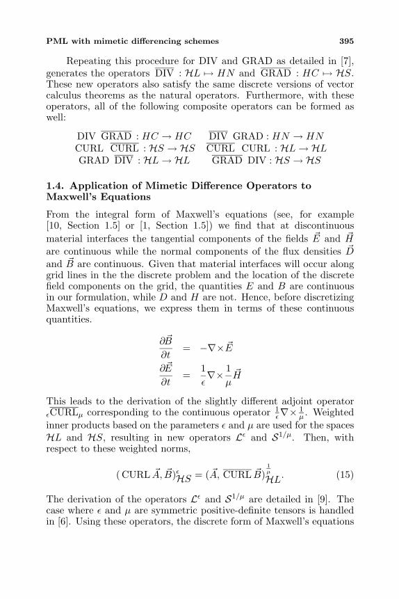
PML with mimetic differencing schemes 395
Repeating this procedure for DIV and GRAD as detailed in [7],generates the operators DIV : HL → HN and GRAD : HC → HS.These new operators also satisfy the same discrete versions of vectorcalculus theorems as the natural operators. Furthermore, with theseoperators, all of the following composite operators can be formed aswell:
DIV GRAD : HC → HC DIV GRAD : HN → HNCURL CURL : HS → HS CURL CURL : HL→ HLGRAD DIV : HL→ HL GRAD DIV : HS → HS
1.4. Application of Mimetic Difference Operators toMaxwell’s Equations
From the integral form of Maxwell’s equations (see, for example[10, Section 1.5] or [1, Section 1.5]) we find that at discontinuousmaterial interfaces the tangential components of the fields E and H
are continuous while the normal components of the flux densities D
and B are continuous. Given that material interfaces will occur alonggrid lines in the the discrete problem and the location of the discretefield components on the grid, the quantities E and B are continuousin our formulation, while D and H are not. Hence, before discretizingMaxwell’s equations, we express them in terms of these continuousquantities.
∂B
∂t= −∇× E
∂E
∂t=
1ε∇× 1
µH
This leads to the derivation of the slightly different adjoint operatorεCURLµ corresponding to the continuous operator 1
ε∇× 1µ . Weighted
inner products based on the parameters ε and µ are used for the spacesHL and HS, resulting in new operators Lε and S1/µ. Then, withrespect to these weighted norms,
( CURL A, B)εHS = ( A, CURL B)1µ
HL. (15)
The derivation of the operators Lε and S1/µ are detailed in [9]. Thecase where ε and µ are symmetric positive-definite tensors is handledin [6]. Using these operators, the discrete form of Maxwell’s equations
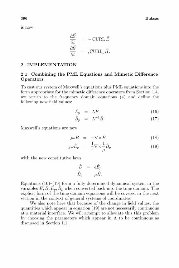
396 Buksas
is now
∂B
∂t= −CURL E
∂E
∂t= εCURLµ
H.
2. IMPLEMENTATION
2.1. Combining the PML Equations and Mimetic DifferenceOperators
To cast our system of Maxwell’s equations plus PML equations into theform appropriate for the mimetic difference operators from Section 1.4,we return to the frequency domain equations (4) and define thefollowing new field values:
Ep = ΛE (16)
Bp = Λ−1B. (17)
Maxwell’s equations are now
jωB = −∇×E (18)
jωEp =1ε∇× 1
µBp (19)
with the new constitutive laws
D = εEp
Bp = µH.
Equations (16)–(19) form a fully determined dynamical system in thevariables E, B, Ep, Bp when converted back into the time domain. Theexplicit form of the time domain equations will be covered in the nextsection in the context of general systems of coordinates.
We also note here that because of the change in field values, thequantities which appear in equation (19) are not necessarily continuousat a material interface. We will attempt to alleviate this this problemby choosing the parameters which appear in Λ to be continuous asdiscussed in Section 1.1.
PML with mimetic differencing schemes 397
2.2. Conversion to the Time Domain
Maxwell’s equations (18, 19) as derived in the previous section, can beconverted back into the time domain as discretized in space to yield
∂B
∂t= −CURL E
∂Ep
∂t= εCURLµBp.
The remaining equations all arise from the PML are involve no spacederivatives.
E = Λ−1η Λ−1
ξ Ep
Bp = Λ−1η Λ−1
ξ B
In our simulations, we consider the transverse electric (TE) mode,which consists of the components Eξ, Eη and Bz. Dropping theequations in which all components are zero and using the definitionsof the matrices Λξ and Λη yields the equations:
Eξ = sξs−1η Ep
ξ (20)
Eη = s−1ξ sηEp
η (21)
Bz = s−1ξ s−1
η Bpz (22)
where Epξ , Ep
η , Bpz are components of Ep and Bp. Equations (20) and
(21) have the general form
Xsα = Y sβ (23)
where aα and sβ are two different complex PML coefficients and X,Y are vector field components. We illustrate the exact procedurefor converting equations of this type into the time domain for sα =κα + σα/ε0jω. Equation (23) becomes(
κα +σα
ε0jω
)X =
(κβ +
σβ
ε0jω
)Y
Multiplying by jω and converting, we obtain,
κα∂X
∂t+
σα
ε0X = κβ
∂Y
∂t+
σβ
ε0Y. (24)
Given that one of the two quantities, ∂X∂t , ∂Y
∂t is determined by otherequations in the dynamical system, (24) can then be solved for theremaining unknown time derivative.
398 Buksas
To discretize equation (22) we introduce an intermediate variable,Bp
z and split it into two equations:
sξBz = Bpz
sηBpz = Bp
z . (25)
These equations can be converted to the time domain by the sameprocess. For our expanded system consisting of Eξ, Eη, Ep
ξ , Epη , Bz, Bp
z
and Bpz , the resulting system of time-domain equations is:
∂B
∂t= −CURL E (26)
∂Ep
∂t= εCURLµ
Bp (27)
∂Eξ
∂t=
1κη
(σξE
pξ − σηEξ + κξ
∂Epξ
∂t
)(28)
∂Eη
∂t=
1κξ
(σηEp
η − σξEη + κη
∂Epη
∂t
)(29)
∂Bpz
∂t= σξBz + κξ
∂Bz
∂t(30)
∂Bpz
∂t= σηBp
z + κη∂Bp
z
∂t(31)
The equations (26), (27) are vector equations for all three componentsof E, B, Ep and Bp. Our TE mode solution only involves three of thesesix equations. The remaining time derivatives in the right-hand-sidesof equations (28) through (31) can be eliminated through substitution.
2.3. Discretization of the Equations
We employ the same staggered time-stepping approach as proposed byYee [19]. In this scheme, the values of the electric field and relatedquantities are updated at integer multiples of the fundamental timestep while the magnetic field and related quantities are updated at themidpoints of the intervals, denoted with the indices n + 1/2. Forwarddifferencing schemes are used for each step of the process with secondorder convergence of the results in time. For our implementation, thequantities Eξ, Eη, Ep
ξ , Epη are defined on the integral multiples of the
time step n. The quantities Bz, Bpz and Bp
z are defined on the midpointsn + 1
2 .
PML with mimetic differencing schemes 399
The discrete form of the equations that we implement here isnot derived directly from the system of equations (26)–(31). Instead,we discretize all of the expressions in the form of equation (24) andequations (25) directly using standard first-order differences for thetime derivatives and the two-point average for the conductivity terms.This yields the following update equation for the discrete quantities:
Xn+1(
σα
2+
κα
∆t
)+Xn
(σα
2− κα
∆t
)=Y n+1
(σβ
2+
κβ
∆t
)+Y n
(σβ
2− κβ
∆t
).
(32)One of the n+1 terms is already known from it’s involvement in otherequations, so this expression is solved for the unknown n+1 term. (Theequation for quantities on the half time intervals is found by adjustingthe indices.)
The main loop of the iteration, illustrating the mutualdependencies of the data, is as follows. We start with current values atthe time steps n and n − 1
2 . Unless otherwise stated, the update ruleis some form of equation (32).
• Compute Bn+ 1
2z from B
n− 12
z and Enx , En
y from Bzn+ 12 = Bzn−
12 −
∆t( CURL E)z.
• Compute Bp,n+ 1
2z from B
p,n− 12
z , Bn− 1
2z and B
n+ 12
z .
• Compute Bp,n+ 1
2z from B
p,n− 12
z , Bp,n− 1
2z and B
p,n+ 12
z .
• Compute Ep,n+1x and Ep,n+1
y from Ep,nx , Ep,n
y and Bp,n+ 1
2z from
Ep,n+1 = Ep,n + ∆t εCURLµBp.
• Compute En+1x from En
x , Ep,nx and Ep,n+1
x .• Compute En+1
y from Eny , Ep,n
y and Ep,n+1y .
3. TEST PROBLEMS AND RESULTS
3.1. Radiation Problem on a Cartesian Grid
Our first test problem uses a small current loop in the ξη plane,implemented as a fictitious magnetic current, to generate a TE modeelectromagnetic pulse. The magnetic current for this and otherexamples below has the Gaussian time signature:
f(t) = e−(t−tc)2/w2(33)
and in this example, we take tc = 1.0 × 10⁻¹⁰ and w = 2.5 × 10⁻¹¹.(We note that at t = 0, f(0) = e−16 ≈ 1.1×10⁻⁷ so we need not worry
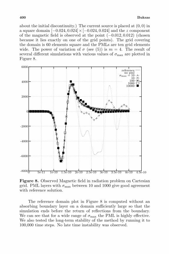
400 Buksas
about the initial discontinuity.) The current source is placed at (0, 0) ina square domain [−0.024, 0.024]× [−0.024, 0.024] and the z componentof the magnetic field is observed at the point (−0.012, 0.012) (chosenbecause it lies exactly on one of the grid points). The grid coveringthe domain is 60 elements square and the PMLs are ten grid elementswide. The power of variation of σ (see (5)) is m = 4. The result ofseveral different simulations with various values of σmax are plotted inFigure 8.
10000100010010
σmax = 10no pml
reference
4.5e-104e-103.5e-103e-102.5e-102e-101.5e-101e-105e-110
6000
4000
2000
0
-2000
-4000
-6000
-8000
Figure 8. Observed Magnetic field in radiation problem on Cartesiangrid. PML layers with σmax between 10 and 1000 give good agreementwith reference solution.
The reference domain plot in Figure 8 is computed without anabsorbing boundary layer on a domain sufficiently large so that thesimulation ends before the return of reflections from the boundary.We can see that for a wide range of σmax the PML is highly effective.We also tested the long-term stability of the method by running it to100,000 time steps. No late time instability was observed.
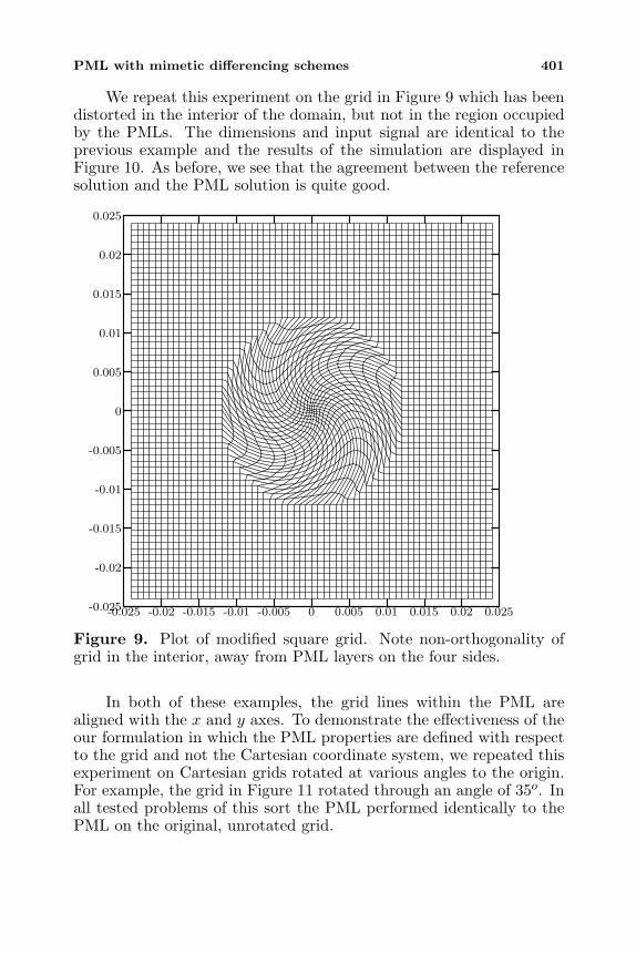
PML with mimetic differencing schemes 401
We repeat this experiment on the grid in Figure 9 which has beendistorted in the interior of the domain, but not in the region occupiedby the PMLs. The dimensions and input signal are identical to theprevious example and the results of the simulation are displayed inFigure 10. As before, we see that the agreement between the referencesolution and the PML solution is quite good.
0.0250.020.0150.010.0050-0.005-0.01-0.015-0.02-0.025
0.025
0.02
0.015
0.01
0.005
0
-0.005
-0.01
-0.015
-0.02
-0.025
Figure 9. Plot of modified square grid. Note non-orthogonality ofgrid in the interior, away from PML layers on the four sides.
In both of these examples, the grid lines within the PML arealigned with the x and y axes. To demonstrate the effectiveness of theour formulation in which the PML properties are defined with respectto the grid and not the Cartesian coordinate system, we repeated thisexperiment on Cartesian grids rotated at various angles to the origin.For example, the grid in Figure 11 rotated through an angle of 35o. Inall tested problems of this sort the PML performed identically to thePML on the original, unrotated grid.
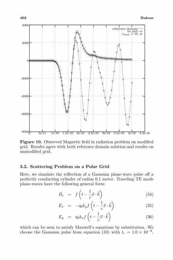
402 Buksas
σmax = 10no pml
reference domain
4.5e-104e-103.5e-103e-102.5e-102e-101.5e-101e-105e-110
4000
2000
0
-2000
-4000
-6000
-8000
Figure 10. Observed Magnetic field in radiation problem on modifiedgrid. Results agree with both reference domain solution and results onunmodified grid.
3.2. Scattering Problem on a Polar Grid
Here, we simulate the reflection of a Gaussian plane-wave pulse off aperfectly conducting cylinder of radius 0.1 meter. Traveling TE modeplane-waves have the following general form:
Bz = f
(t− 1
cx · k
)(34)
Ex = −η0kyf
(t− 1
cx · k
)(35)
Ey = η0kxf
(t− 1
cx · k
)(36)
which can be seen to satisfy Maxwell’s equations by substitution. Wechoose the Gaussian pulse from equation (33) with tc = 1.0 × 10⁻⁹,
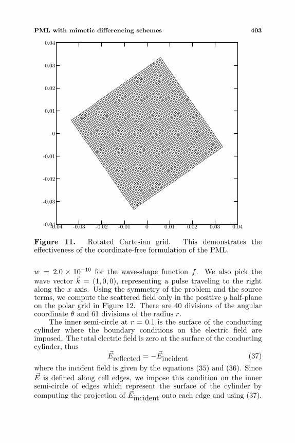
PML with mimetic differencing schemes 403
0.040.030.020.010-0.01-0.02-0.03-0.04
0.04
0.03
0.02
0.01
0
-0.01
-0.02
-0.03
-0.04
Figure 11. Rotated Cartesian grid. This demonstrates theeffectiveness of the coordinate-free formulation of the PML.
w = 2.0 × 10⁻¹⁰ for the wave-shape function f . We also pick thewave vector k = (1, 0, 0), representing a pulse traveling to the rightalong the x axis. Using the symmetry of the problem and the sourceterms, we compute the scattered field only in the positive y half-planeon the polar grid in Figure 12. There are 40 divisions of the angularcoordinate θ and 61 divisions of the radius r.
The inner semi-circle at r = 0.1 is the surface of the conductingcylinder where the boundary conditions on the electric field areimposed. The total electric field is zero at the surface of the conductingcylinder, thus
Ereflected = − Eincident (37)
where the incident field is given by the equations (35) and (36). SinceE is defined along cell edges, we impose this condition on the innersemi-circle of edges which represent the surface of the cylinder bycomputing the projection of Eincident onto each edge and using (37).
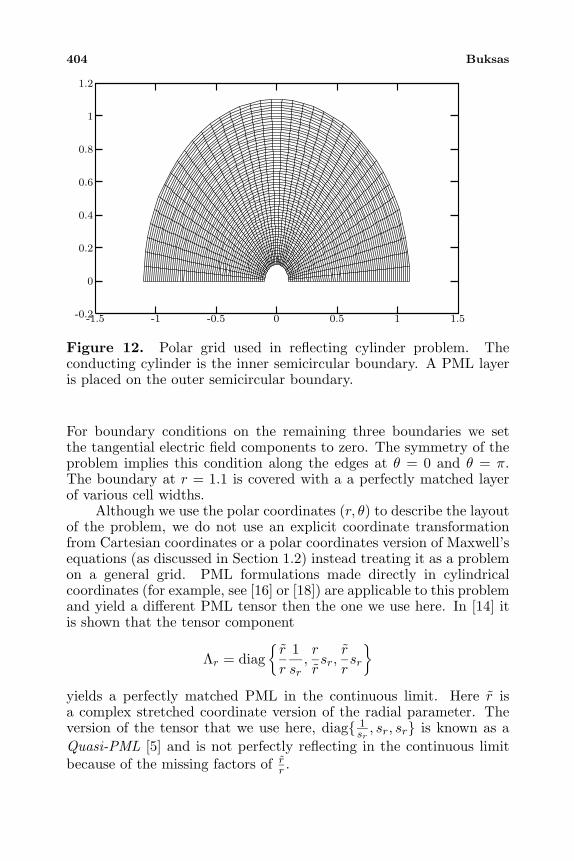
404 Buksas
1.510.50-0.5-1-1.5
1.2
1
0.8
0.6
0.4
0.2
0
-0.2
Figure 12. Polar grid used in reflecting cylinder problem. Theconducting cylinder is the inner semicircular boundary. A PML layeris placed on the outer semicircular boundary.
For boundary conditions on the remaining three boundaries we setthe tangential electric field components to zero. The symmetry of theproblem implies this condition along the edges at θ = 0 and θ = π.The boundary at r = 1.1 is covered with a a perfectly matched layerof various cell widths.
Although we use the polar coordinates (r, θ) to describe the layoutof the problem, we do not use an explicit coordinate transformationfrom Cartesian coordinates or a polar coordinates version of Maxwell’sequations (as discussed in Section 1.2) instead treating it as a problemon a general grid. PML formulations made directly in cylindricalcoordinates (for example, see [16] or [18]) are applicable to this problemand yield a different PML tensor then the one we use here. In [14] itis shown that the tensor component
Λr = diag
r
r
1sr
,r
rsr,
r
rsr
yields a perfectly matched PML in the continuous limit. Here r isa complex stretched coordinate version of the radial parameter. Theversion of the tensor that we use here, diag 1
sr, sr, sr is known as a
Quasi-PML [5] and is not perfectly reflecting in the continuous limitbecause of the missing factors of r
r .
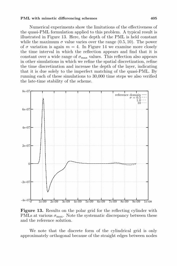
PML with mimetic differencing schemes 405
Numerical experiments show the limitations of the effectiveness ofthe quasi-PML formulation applied to this problem. A typical result isillustrated in Figure 13. Here, the depth of the PML is held constantwhile the maximum σ value varies over the range (0.5, 10). The powerof σ variation is again m = 4. In Figure 14 we examine more closelythe time interval in which the reflection appears and find that it isconstant over a wide range of σmax values. This reflection also appearsin other simulations in which we refine the spatial discretization, refinethe time discretization and increase the depth of the layer, indicatingthat it is due solely to the imperfect matching of the quasi-PML. Byrunning each of these simulations to 30,000 time steps we also verifiedthe late-time stability of the scheme.
101.0
σ = 0.5reference domain
1e-089e-098e-097e-096e-095e-094e-093e-092e-091e-090
8e-07
6e-07
4e-07
2e-07
0
-2e-07
-4e-07
Figure 13. Results on the polar grid for the reflecting cylinder withPMLs at various σmax. Note the systematic discrepancy between theseand the reference solution.
We note that the discrete form of the cylindrical grid is onlyapproximately orthogonal because of the straight edges between nodes
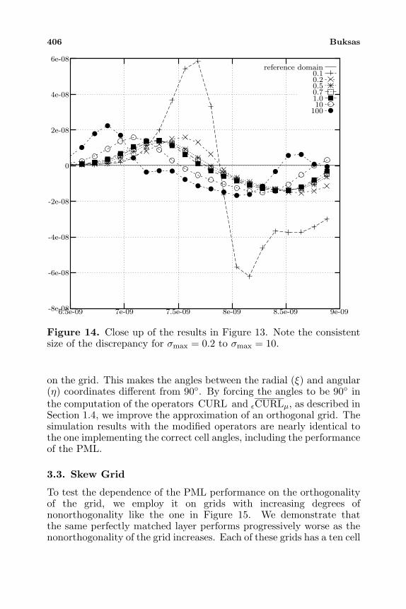
406 Buksas
100101.00.70.50.20.1
reference domain
9e-098.5e-098e-097.5e-097e-096.5e-09
6e-08
4e-08
2e-08
0
-2e-08
-4e-08
-6e-08
-8e-08
Figure 14. Close up of the results in Figure 13. Note the consistentsize of the discrepancy for σmax = 0.2 to σmax = 10.
on the grid. This makes the angles between the radial (ξ) and angular(η) coordinates different from 90. By forcing the angles to be 90 inthe computation of the operators CURL and εCURLµ, as described inSection 1.4, we improve the approximation of an orthogonal grid. Thesimulation results with the modified operators are nearly identical tothe one implementing the correct cell angles, including the performanceof the PML.
3.3. Skew Grid
To test the dependence of the PML performance on the orthogonalityof the grid, we employ it on grids with increasing degrees ofnonorthogonality like the one in Figure 15. We demonstrate thatthe same perfectly matched layer performs progressively worse as thenonorthogonality of the grid increases. Each of these grids has a ten cell
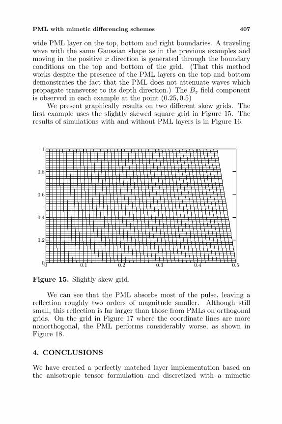
PML with mimetic differencing schemes 407
wide PML layer on the top, bottom and right boundaries. A travelingwave with the same Gaussian shape as in the previous examples andmoving in the positive x direction is generated through the boundaryconditions on the top and bottom of the grid. (That this methodworks despite the presence of the PML layers on the top and bottomdemonstrates the fact that the PML does not attenuate waves whichpropagate transverse to its depth direction.) The Bz field componentis observed in each example at the point (0.25, 0.5)
We present graphically results on two different skew grids. Thefirst example uses the slightly skewed square grid in Figure 15. Theresults of simulations with and without PML layers is in Figure 16.
0.50.40.30.20.10
1
0.8
0.6
0.4
0.2
0
Figure 15. Slightly skew grid.
We can see that the PML absorbs most of the pulse, leaving areflection roughly two orders of magnitude smaller. Although stillsmall, this reflection is far larger than those from PMLs on orthogonalgrids. On the grid in Figure 17 where the coordinate lines are morenonorthogonal, the PML performs considerably worse, as shown inFigure 18.
4. CONCLUSIONS
We have created a perfectly matched layer implementation based onthe anisotropic tensor formulation and discretized with a mimetic
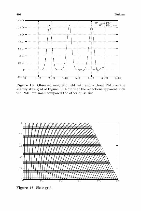
408 Buksas
With PMLWithout PML
7e-096e-095e-094e-093e-092e-091e-090
1.4e-06
1.2e-06
1e-06
8e-07
6e-07
4e-07
2e-07
0
-2e-07
Figure 16. Observed magnetic field with and without PML on theslightly skew grid of Figure 15. Note that the reflections apparent withthe PML are small compared the other pulse size.
0.50.40.30.20.10
1
0.8
0.6
0.4
0.2
0
Figure 17. Skew grid.
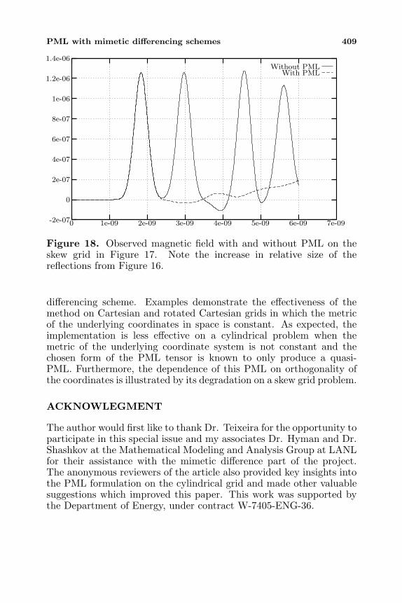
PML with mimetic differencing schemes 409
With PMLWithout PML
7e-096e-095e-094e-093e-092e-091e-090
1.4e-06
1.2e-06
1e-06
8e-07
6e-07
4e-07
2e-07
0
-2e-07
Figure 18. Observed magnetic field with and without PML on theskew grid in Figure 17. Note the increase in relative size of thereflections from Figure 16.
differencing scheme. Examples demonstrate the effectiveness of themethod on Cartesian and rotated Cartesian grids in which the metricof the underlying coordinates in space is constant. As expected, theimplementation is less effective on a cylindrical problem when themetric of the underlying coordinate system is not constant and thechosen form of the PML tensor is known to only produce a quasi-PML. Furthermore, the dependence of this PML on orthogonality ofthe coordinates is illustrated by its degradation on a skew grid problem.
ACKNOWLEGMENT
The author would first like to thank Dr. Teixeira for the opportunity toparticipate in this special issue and my associates Dr. Hyman and Dr.Shashkov at the Mathematical Modeling and Analysis Group at LANLfor their assistance with the mimetic difference part of the project.The anonymous reviewers of the article also provided key insights intothe PML formulation on the cylindrical grid and made other valuablesuggestions which improved this paper. This work was supported bythe Department of Energy, under contract W-7405-ENG-36.
410 Buksas
REFERENCES
1. Balanis, C. A., Advanced Engineering Electromagnetics, JohnWiley & Sons, New York, 1989.
2. Berenger, J.-P., “A perfectly matched layer for the absorptionof electromagnetic waves,” Journal of Computational Physics,Vol. 114, 185–200, October 1994.
3. Gedney, S. D., “An anisotropic perfectly matched layer-absorbingmedium for the truncation of FDTD lattices,” IEEE Transactionson Antennas and Propagation, Vol. 44, No. 12, 1630–1639,December 1996.
4. Gedney, S. D., “An anisotropic PML absorbing media forthe FDTD simulation of fields in lossy and dispersive media,”Electromagnetics, Vol. 16, 399–415, 1996.
5. He, J.-Q. and Q. H. Liu, “A nonuniform cylindrical FDTDalgorithm with improved PML and quasi-PML absorbingboundary conditions,” IEEE Transactions on Geoscience andRemote Sensing, Vol. 37, No. 2, 1066–1072, March 1999.
6. Hyman, J., M. Shashkov, and S. Stienberg, “The numericalsolution of diffusion problems in strongly heterogeneous non-isotropic materials,” Journal of Compuational Physics, Vol. 132,130–148, 1997.
7. Hyman, J. M. and M. Shashkov, “Adjoint operators for thenatural discretizations of the divergence, gradient and curl onlogically rectangular grids,” Applied Numerical Mathematics,Vol. 25, 413–442, 1997.
8. Hyman, J. M. and M. Shashkov, “Natural discretizations forthe divergence, gradient and curl on logically rectangular grids,”Applied Numerical Mathematics, Vol. 33, No. 4, 81–104, 1997.
9. Hyman, J. M. and M. Shashkov, “Mimetic discretizations forMaxwell’s equations,” Journal of Compuational Physics, Vol. 151,881–909, 1999.
10. Jackson, J. D., Classical Electrodynamics, 2nd edition, JohnWiley & Sons, New York, 1975.
11. Mittra, R. and U. Pekel, “A new look at the perfectlymatched layer (PML) concept for the reflectionless absorptionof electromagnetic waves,” IEEE Microwave and Guided WaveLetters, Vol. 5, No. 3, 84–86, March 1995.
12. Sacks, Z. S., D. M. Kingsland, R. Lee, and J.-F. Lee, “A perfectlymatched anisotropic absorber for use as an absorbing boundarycondition,” IEEE Transactions on Antennas and Propagation,
PML with mimetic differencing schemes 411
Vol. 43, No. 12, 1460–1463, December 1995.13. Taflove, A. (ed.), Advances in Computational Electrodynamics.
The finite-difference time-domain method, Artech House, Boston,Mass., 1998.
14. Teixeira, F. L. and W. C. Chew, “Systematic derivation ofanisotropic PML absorbing media in cylindrical and sphericalcoordinates,” IEEE Microwave and Guided Wave Letters,Vol. 7, No. 11, 371–373, November 1997.
15. Teixeira, F. L. and W. C. Chew, “A general approach toextend Berenger’s absorbing boundary condition to anisotropicand dispersive media,” IEEE Transactions on Antennas andPropagation, Vol. 46, No. 9, 1386–1387, September 1998.
16. Teixeira, F. L. and W. C. Chew, “PML-FDTD in cylindricaland spherical grids,” IEEE Microwave and Guided Wave Letters,Vol. 7, No. 9, 285–287, September 1997.
17. Tong, M.-S., Y. Chen, M. Kuzuoglu, and R. Mittra, “A newanisotropic perfectly matched layer medium for mesh truncationin finite difference time domain analysis,” Int. J. Electronics,Vol. 86, No. 9, 1085–1091, 1999.
18. Yang, B. and P. G. Petropoulos, “Plane-wave analysis andcomparison of split-field, biaxial and uniaxial PML methodsas ABC’s for pseudospectral electromagnetic wave simulationsin curvilinear coordinates,” Journal of Computational Physics,Vol. 146, 747–774, 1998.
19. Yee, K. S., “Numerical solution of initial boundary valueproblems involving Maxwell’s equations in isotropic media,” IEEETransactions on Antennas and Propagation, Vol. 14, 302–307,1966.
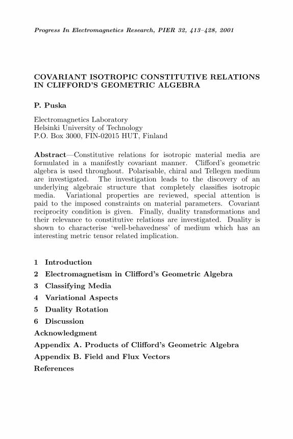
Progress In Electromagnetics Research, PIER 32, 413–428, 2001
COVARIANT ISOTROPIC CONSTITUTIVE RELATIONSIN CLIFFORD’S GEOMETRIC ALGEBRA
P. Puska
Electromagnetics LaboratoryHelsinki University of TechnologyP.O. Box 3000, FIN-02015 HUT, Finland
Abstract—Constitutive relations for isotropic material media areformulated in a manifestly covariant manner. Clifford’s geometricalgebra is used throughout. Polarisable, chiral and Tellegen mediumare investigated. The investigation leads to the discovery of anunderlying algebraic structure that completely classifies isotropicmedia. Variational properties are reviewed, special attention ispaid to the imposed constraints on material parameters. Covariantreciprocity condition is given. Finally, duality transformations andtheir relevance to constitutive relations are investigated. Duality isshown to characterise ‘well-behavedness’ of medium which has aninteresting metric tensor related implication.
1 Introduction
2 Electromagnetism in Clifford’s Geometric Algebra
3 Classifying Media
4 Variational Aspects
5 Duality Rotation
6 Discussion
Acknowledgment
Appendix A. Products of Clifford’s Geometric Algebra
Appendix B. Field and Flux Vectors
References
414 Puska
1. INTRODUCTION
Maxwell equations are usually supplemented by constitutive relations,for these provide the information about the surrounding medium. Inthe Minkowski space constitutive relations take the bivector (or 2-form)F ∼ (E,B), and map it to the bivector (2-form) G ∼ (H,D).
However, given their importance in practical problem solving,constitutive relations as well as their representations are lessfrequently explained in physics textbooks than what one might expect.Constitutive relations appear to be more or less a engineer’s cup of tea,for it is usually antenna and microwave engineering oriented worksthat discuss them (see for example the numerous references listed in[1]). As these works describe constitutive relations within the Gibbs–Heaviside vector algebra requiring an inertial frame to be specified,physicists have not adopted them widely. Therefore we look for acovariant description that satisfies the engineer and the physicist alike.The Minkowski space is of course the space to be used, for constitutiverelations suggest that Maxwell equations are covariant under Lorentztransformations [2, 3]. In this study we give manifestly covariantrepresentations of a few important isotropic media and discuss theirimplications. We also hope that the geometric substance of constitutiverelations becomes more apparent with our treatment. To convey this‘geometricity’ of constitutive relations more efficiently we adopt thelanguage of Clifford’s geometric algebra, which we will introduce inSection 2. The practical results are given in the examples in Section 3.For the benefit of more theoretically inclined readers, we discuss brieflyvariational aspects in Section 4 and duality properties in Section 5. Theunderlying algebraic structure is exposed in the end of Section 3, andthe reciprocity conditions are reviewed in the latter part of Section 4.
2. ELECTROMAGNETISM IN CLIFFORD’SGEOMETRIC ALGEBRA
Constitutive relations are much easier to write down explicitly, if theyare assumed to be linear, and this is normally done in the literature [3].We make that assumption too. Furthermore, we discard the distinctionbetween vectors and forms, for we work entirely within a known metric.This identification of vectors with their duals makes the Clifford’sgeometric algebra –or Clifford algebra for short– an obvious choicefor our working environment. We work within an algebra generated by
Covariant isotropic constitutive relations 415
basis vectors e1 . . . e4 with the relations 1
e21 = e2
2 = e22 = 1, e4 = −1
eλeν = −eνeλ for λ = ν.
This algebra bears the label C3,1, which means that three of the basisvectors have norm 1 and the remaining one has −1. For a quickreference, we have explained in Appendix A the different productsof Clifford algebra. Some reading suggestions are also listed there.
The electromagnetic field can be written as two bivectors2 F andG
F =12F λνeλν , G =
12Gλνeλν , (1)
where we have used the summation convention. F and G satisfyMaxwell equations
∂ ∧ F = 0, (2)∂ ∧G = J (3)
where Dirac operator ∂, when given in its space–and–time-componentform, reads ∂ = (∇ − c−1e4 ∂t). J is a trivector representing electriccharges and currents.
Constitutive relations in the context of Clifford algebra have beendiscussed earlier by Hillion in ref. [6], but his approach differs fromours, being concerned with the well-posedness of the problem. We willfocus on the algebraic properties of the constitutive operator.
The constitutive operator χ maps F to G:
G = χ F. (4)
The reason why we mark χ with the accent ˘ will become clear in amoment.
The case of isotropic media may look simple, but there is in factmore than one way to connect F to G. Therefore χ must be constructedin a manner that allows such a diverse media as the familiar dielectricmaterials and the exotic chiral and Tellegen materials to be equally wellrepresented. Even in the absence of polarisable materials there remainsa constitutive map, namely the vacuum constitutive map. The origin1 The notation we use is mainly borrowed from ref. [9]: Vectors and basis multivectors, e.g.e1e2 = e12, are in boldface, but we deviate from ref. [9] by denoting all other multivectorswith unslanted caps, e.g. F, G, I. Scalars and unspecified elements of algebra are both inlowercase, e.g. c, u, but it should be clear from the context which ones are meant. Ref. [5]uses identical notation.2 In this paper we do not observe the difference between inner and outer orientations. Fornice pictorial expositions, see [4].
416 Puska
of this map might be the metric itself [3, 7], but in our case it sufficesto say that the metric transforms F to G via the Hodge mapping [8,p. 28]:
G =√
ε0µ0
F, (5)
where the Hodge mapping has the explicit form
F = F I. (6)
The factor I gives the orientation of the space in a form of orientedvolume element, in C3,1 I = e1e2e3e4. The ‘tilde’ operation reversesthe order of elements in Clifford products [9, pp. 14–15], e.g. (e123 +e1)∼ = e321 +e1. In the Minkowski space the Hodge operation has theclosure property = −id when operating on bivectors.
We find the Hodge mapping to be convenient in relating differentformulations of Maxwell equations. The formulation that Post in ref.[3, pp. 53–56] adopts can translated to our notation as follows:
∂ ∧ F = 0, ∂ G = J,
where G = − G and G = G. For sources, J = − J and J = − J.The constitutive mapping χ takes the bivector F to the bivector G:
G = χF.
Comparison with (4) gives the relation
χ = χ.
Hodge mapping makes also an appearance in the so-called dualityrotation
F′ = cosα F + sinα F, (7)
which leaves the source-less vacuum Maxwell equations as well as thevacuum energy–momentum tensor invariant. Here α has no simplegeometric interpretation, it gives just a measure of the amount of therotation that the field has undergone in the abstract space of (F, F).The importance of duality rotation was probably first appreciatedin the 20’s by Rainich [10], and later elaborated and put in to abroader context by Misner and Wheeler [11]. In addition to theinvariance property above, the duality rotation comes in handy whencharacterising media.
Covariant isotropic constitutive relations 417
3. CLASSIFYING MEDIA
We are of course aware that an isotropic polarisable medium becomesbi-anisotropic when observed in a frame where the medium appearsto be moving [19, pp. 594–595], and in order that we can give acovariant description of isotropy, we define an isotropic medium tobe a medium, where the only discriminate direction is the medium’sfour-velocity. The definition works well in a macroscopic scale, butbecomes rather impractical in the other end of the scale, where wehave difficulties to distinguish between random thermal movementsand externally induced displacements.
The role of four-velocity is best explained by studying a fewexamples, which also serve as a basis of our classification of media:
Magneto–dielectric medium
Basic isotropic magneto–dielectric medium has a constitutive relationof the form
G =12(c ε + c−1µ−1) F +
12
(c ε− c−1µ−1)w−1 F w, (8)
where w = γ v + γ c e4 is the four-velocity of the medium, relativevelocity v ∈ R3 and γ = 1/
√1− v2/c2. When the medium appears to
be stationary, the presently co-moving observer sets w = c e4 in (8)and thus recovers the usual magneto–dielectric constitutive relations
G =12(c ε + c−1µ−1) F +
12
(c ε− c−1µ−1)e−14 F e4, (9)
or in a traditional form (cf. Appendix 6) D = εE, H = 1µ B.
In this particular case the term e−14 Fe4, or reflection of F with
respect to e4, on the right hand side of (9) can be interpreted as aspace conjugation (inversion) sending
eiej → (−ei)(−ej) = eiej , eie4 → (−ei)e4 = −eie4
where i, j ∈ 1, 2, 3.In passing, we note that it was probably Jauch and Watson in 1948
who first wrote magneto–dielectric medium’s constitutive relations inthe form where the medium’s four-velocity appears explicitly, eqn. 9 inref. [12]. Thus our (8) can be viewed as a Clifford algebra version oftheir equation. Their constitutive relations, written in index notation,have appeared in some textbooks, e.g. [13].
418 Puska
We can bring relations (8) into an even neater form, for
w−1(w−1Fw)w = rw(rwF) = rwrwF = F,
which means that algebraically reflections with respect to w, denotedas rw, behave like the so-called unipodal numbers [15], viz. rwrw = 1.We can then immediately conceive functions with unipodal arguments,especially exponential ones:
exp(rwφ) = coshφ + rw sinhφ. (10)
As a natural consequence of these observations, we define
coshφ =12(εr + µ−1
r ), sinhφ =12(εr − µ−1
r ), (11)
and thus (8) becomes
G =1η0
erwφ F, η0 =√
µ0/ε0 (12)
Chiral medium
Isotropic chiral medium contains handed inclusions of similarhandedness mixed randomly in a host material (racemic mixturesare not considered here). These inclusions effect a coupling betweendynamic electric and magnetic fields. We write the correspondingconstitutive relations as
G =1η0
erwφF + Ξ rwF. (13)
Here Ξ is an operator, which in 3D formulation involves a timederivative [14]. What kind of time derivative should Ξ contain, if allthe observers are to concur with it? Luckily, we do have a commontime standard, the proper time τ . We write
Ξ = ξ∂
∂τ= ξ∂τ , (14)
where ξ is a parameter measuring the strength of chirality.In traditional 3D formulations of electromagnetism we have tacitly
assumed a harmonic time variance, which suggests the use of quantitiessuch as jω or j in (14), but here we are working in a geometric algebra,and hence every quantity must have a geometric content. We couldconsider a structure like C ⊗ C3,1, and thus readily adopt j from 3D
Covariant isotropic constitutive relations 419
theory, but the imaginary numbers introduced in this way have no cleargeometric meaning. On the other hand, C3,1 itself contains severalcopies of complex fields, i.e. fields with generators
1, e23, 1, e31, 1, e23, 1, e123, 1, e1234,
and these should be considered as possible substitutes for thetraditional complex numbers. The choice turns out to be particularlysimple in the case of circularly polarised waves. Suppose that xis a space–time position and k a (constant) wave four-vector, thenthe circularly polarised plane wave solution of homogeneous Maxwellequations becomes
F(x · k) = e±I(k·x)F0 (15)
where F0 is a constant bivector, I = e1234, and ± signifies the twopossible helicities. Hence
∂τF(x · k) = ±e±I(k·x)I ∂τ (x · k)F0 = ±e±I(k·x)I (w · k)F0
= ±I (w · k) e±I(k·x)F0 = ±I (w · k) F(x · k). (16)
Therefore we find it convenient to set ∂τ = ±(w ·k) I. The sign shouldbe chosen to reflect the correct handedness. e1234 is a good candidatefor an ’imaginary number’ in view of the fact it is also a Lorentz-invariant.
Comparing now (6) and (14) shows that for circularly polarisedwaves Hodge and chirality operator are almost the same operator. Thisaffects the Euler–Lagrange equations as we shall see later.
Tellegen medium
In 1948 Tellegen [16] introduced a new device for electric circuits:the gyrator, which ’gyrated’ a current into a voltage and vice versa.Tellegen also suggested that such a device could be made of materialwith relations
D = ε′E + γH, B = µH + γE, γ2 ≈ εµ,
which translates to
G =1η0
erwφ F + ψ F, (17)
in our covariant notation. Here ε = ε′ − γ2/µ and ψ = γ/µ [1, p. 309].We will discover in Section 4 how the ’Post-constraint’ [3, eqn. (6.18)]results from (17).
420 Puska
Algebraic structure
When we look at the forms of (8), (13) and (17) a pattern begins toemerge: a most general isotropic medium has the form
G = a1 F + a2 rwF + a3 F + a4 rw F. (18)
Clearly, we have exhausted all possible combinations of and rw, whichwe take to be basis vectors of a new, induced algebra. Not surprisingly,this new algebra is of Clifford variety, since it is generated by , rwwith relations
rw = −rw , r2w = 1, 2 = −1,
i.e. we have here C1,1 (the unipodal number system mentioned aboveis in fact C1,0 and is contained in C1,1). Thus all isotropic media canbe classified by the four-dimensional algebra C1,1.
4. VARIATIONAL ASPECTS
Let us briefly investigate variational implications of our constitutiverelations. For a moment, assume that Ξ behaves like a scalar (i.e.commutes with every element of algebra). Moreover, assume that (2)implies
F = ∂ ∧A, (19)
where A is a four-potential and thus the Lagrangian of theelectromagnetic field with sources is a quadrivector
L =12(∂ ∧A) ∧G(A)−A ∧ J, (20)
where G assumes the form (we use Thirring’s Lagrangian [17, p. 46]with suitable modifications)
G(A) = ψ ∂ ∧A + Ξ rw∂ ∧A +1η0
erwφ ∂ ∧A. (21)
To be precise, our assumption (19) is true only for star-like regions [18,pp. 38–46], but this should not be too restricting, for we can considerregions that are locally star-like.
Variation A→ A + δA gives
δW =∫
dV[ δA ∧ ∂ ∧ (1η0
erwφ ∂ ∧A)− δA ∧ J
Covariant isotropic constitutive relations 421
+∂ ∧ (δA1η0
erwφ ∂ ∧A) + ψ ∂ ∧ (A ∧ ∂ ∧ δA) ]
=∫VdV δA ∧ (∂ ∧ 1
η0erwφ ∂ ∧A− J)
+∮∂V
dS δA1η0
erwφ ∂ ∧A +∮∂V
dSψ δA ∧ ∂ ∧A .
In above we made use of Stokes’ theorem∫VdV∂ ∧ f =
∮∂V
dS f, (22)
where dV is of grade n and f is any multivector valued function ofgrade n− 1. Here n = 4, dV = dx dy dz cdt I = dx dy dz cdt e1234, anddS is an oriented differential surface element of grade n− 1 = 3 and ofcompatible orientation [9, p. 261]. Note that δW is a scalar quantity.Furthermore, we have used identities
A ∧ B = B ∧ A, (23)A ∧ rwB = −B ∧ rwA, (24)
A ∧ rw B = B ∧ rw A, (25)
whenever A and B are any bivectors in C3,1. The second and thirdrelation are peculiarities of dimension n = 4, while the first is valid forany pair of multivectors of similar, homogeneous degree and for anydimension [20, pp. 121–122].
We immediately notice that chirality does not contribute to thevariation of the action W , and in fact this can be seen already from(21), because (∂∧A)∧rw(∂∧A) = 0 for any vectors A,w ∈ C3,1. ThusΞ has to more be than just a scalar and chirality –as is well-known–a non-instantaneous effect. Making a substitution Ξ→ ±ξ(w · k)e1234
would immediately correct the situation. The chiral term would thengive a non-vanishing contribution to the volume integral.
If the variation is to vanish for all δA with a boundary valueδA|∂V = 0, the integrand of the volume integral must satisfy
∂ ∧ 1η0
erwφ F− J = 0, (26)
and thus (3) is recovered (the surface integrals over ∂V do notcontribute to (26) due to the condition δA|∂V = 0). As the chiraland Tellegen parameter do not appear in (26) Post concluded thatfor instantaneous and local effects it is economical to demand thatχ[λνσκ] = 0, or to put it differently, it does no harm to set Ξ = ψ = 0,when Ξ and ψ are scalar quantities.[3, Ch. VI, §2]
422 Puska
However, this may not be the complete story. It should be notedthat from the set of electromagnetic Lagrangians we picked just onepossible Lagrangian, other choices could have been made. Our choicewas dictated by convenience and tradition. Furthermore, we have notdiscussed Noether currents. There might still be contribution to theconserved observables as noted by Thirring in Remarks (2.1.6) and(2.1.8) of [17]. The contribution to the canonical energy–momentumtensor is proportional to ∂ ∧ ((e A) ∧ F), where e is a vector fieldgenerating the Lie derivatives. The term is unfortunately gauge–dependent. The meaning and significance of such a term should beduly investigated.
Reciprocity
We conclude this section by briefly checking the reciprocity propertiesof our constitutive mapping χ. The covariant form of reciprocitycondition for fields F and G is∫
VdV(Fa ∧ rwGb − Fb ∧ rwGa) = 0, (27)
which corresponds to the condition (15) in [19, p. 402]. As before, wis the medium’s four-velocity. Now set
Ga,b = ψ Fa,b + Ξ rwFa,b +1η0
erwφ Fa,b, (28)
where Ξ may be a scalar or a scalar multiple of I, and use the conditions(23)–(25). The integrand reduces to
Fa ∧ rwψFb − Fb ∧ rwψFa = 2ψ Fa ∧ rwψFb = 0,
therefore a medium with a Tellegen parameter present is not reciprocal.
5. DUALITY ROTATION
We return now to the duality rotation mentioned earlier. The generalduality transformation is of the form
(F′G′
)=
(a bc d
) (FG
), (29)
where a, b, c, d are just scalars. The associated general linear dualitygroup can be restricted with the vacuum constitutive relations [2, Ch.
Covariant isotropic constitutive relations 423
9]: Set G = η−10 F and assume that the relation holds for duality
transformed fields, G′ = η−10 F′, hence
(F′
η−10 F′
)=
(a bc d
) (F
η−10 F
), (30)
substitute F′ in η−10 F′ and use the closure property = −id. In
addition to that, we want the energy–momentum tensor to be invariant[11], so we choose the determinant of the matrix to be = 1. After re-parametrisation we get
(F′G′
)=
(cosα η0 sinα
−η−10 sinα cosα
) (FG
). (31)
Upon examination of (8), (13) and (17) we note that chiral andmagneto–dielectric constitutive relations behave essentially like theHodge mapping, that is, they have a similar closure property:
χχ = −a2 id. (32)
where a is a scalar factor with a dimension of admittance. However,Tellegen medium does not behave so nicely: application of χ twicedoes not lead to identity (modulo a scalar factor). Thus chiral mediumand magneto–dielectric medium can always be incorporated in a newdual operator, denote it with ′, and a general isotropic constitutivemapping χ can be split in two
χ = a ′ +ψ, (33)
where ′′ = −id., and ψ is the Tellegen parameter. In otherwords, chiral parameter can be duality rotated away, whereas Tellegenparameter not. This can be demonstrated by a straightforwardcalculation: Transform both the fields and constitutive operator ofthe Tellegen medium
G′ = (cosα + sinα)(1η0
erwφ +ψ)(cosα− sinα) F′,
after some easy manipulations (remember that we can now use C1,1)
G′ =1η0
coshφF′+1η0
sinhφ sin 2α rwF′+1η0
sinhφ cos 2α rwF′+ψ F′,
whence it follows that there is no α which makes the Tellegen parameterdisappear.
424 Puska
6. DISCUSSION
We saw that constitutive relations of isotropic medium give rise toan induced Clifford algebra C1,1. It is tempting to think that othermore complicated media induce these kind of algebraic structures. Asa consequence, it would be possible to classify media by the algebrasthey induce. It is probably obvious but we nevertheless point out thatthe classification of more general media involves higher dimensionalalgebras. On the other hand, we noticed that constitutive mappingsof reciprocal and non-reciprocal media do not behave similarly, whichsuggests that we could use this as an alternative way of classifyingmedia. Remembering that the reciprocity was related to the closureproperty of constitutive mapping we can divide general isotropic mediain two classes, those that satisfy this property and those that donot. This observation has some implications, for there is interestingtheory originating from the study of Yang–Mills-fields that says thatgiven a duality operator we can find a corresponding conformal classof metric [21, 22]. The duality operator has to be sufficiently well-behaved, among the requirements we find that the closure propertyshould be satisfied. Therefore magneto–dielectric medium as well aschiral medium can be embedded in the (symmetric) metric tensor, butTellegen medium does not fit in.
Doubtless an alert reader has noticed that Tellegen medium hasbeen a subject of controversy for some time. Those who have missedthis discussion are referred to paper [23] and correspondence [24], forinstance. We hope that the variational derivation and the remarkspresented above have given new ideas.
ACKNOWLEGMENT
The author has benefited from discussions with prof. S. Tretyakovand prof. P. Lounesto. This work has been supported by a NokiaFoundation grant.
APPENDIX A. PRODUCTS OF CLIFFORD’SGEOMETRIC ALGEBRA
The Clifford product of a vector x and any element u of Clifford algebracan be written as
xu = x u + x ∧ u,
where denotes the left contraction and ∧ the exterior product. Thesedecrease and increase the grade, respectively. The left contraction can
Covariant isotropic constitutive relations 425
be defined by its characteristic properties [9, Ch. 3, Ch. 22]
x y = 〈x,y〉,x (u ∧ v) = (x u) ∧ v + u ∧ (x v),(u ∧ v) w = u (v w),
where 〈 , 〉 denotes an inner product which in this work is chosen to bethe usual dot product. Here we have also introduced a ’hat’-operation,grade involution, which is an automorphism that reverses the directionof every vector, for instance
(e1e2e3) = e1e2e3 = (−e1)(−e2)(−e3) = −e1e2e3.
Contraction has an important ’duality’ property relating it to theexterior product:
u v = (u ∧ (v I)) I−1,
where I is the highest grade element of the algebra, e.g. in C3,1I = e1234.
Of course, there exist a right contraction as well, but for thiswork the left contraction is quite sufficient. See [9, Ch. 3] for theproperties of .
The exterior product and the left contraction can be reconstructedfrom the Clifford product
x ∧ u =12
(xu + ux) , x u =12
(xu− ux) .
These reconstructions are from Riesz’s lecture notes, [25, pp.61–67], which is also a good classic introduction (albeit notationallyold-fashioned) to Clifford algebra. For a modern introduction, onemight want to check Lounesto’s review [9]. Clifford algebra inelectrodynamics is developed carefully in refs. [26, 27]. Standardreferences for Clifford algebra are [28, 29].
It is sometimes of interest to translate Clifford algebra productsto Gibbs–Heaviside vector calculus products. In order to do that, wehave to single out an inertial system, as explained in 6. Then we canfind the following relations between the cross product and the exteriorproduct (now I = e123):
x× y = (x ∧ y) I−1, x ∧ y = (x× y) I.
APPENDIX B. FIELD AND FLUX VECTORS
The electric field vector E can be found from F by choosing a particularframe and measuring the electric field in that frame. As an algebraic
426 Puska
procedure this amounts to choosing a basis V ′, identification of e4 ∈ V ′
with the observer, and left contracting F by c e4:
E = c e4 F.
The procedure can be repeated to yield H from G
H = c e−14 G = −c e4 G.
Electric and magnetic flux densities are a bit trickier, here we also haveto invoke the duality of vectors and trivectors:
B = (e−14 ∧ F), D = (e−1
4 ∧G).
Thus in an inertial frame F and G can be decomposed as3
F =Ece4 −Be123, G = −H
ce4 −De123.
We can say that we have split F and G in space and time components.Similarly, for G we can write
G = De4 −Hc
e123.
REFERENCES
1. Lindell, I., A. H. Sihvola, S. A. Tretyakov, and A. J. Viitanen,Electromagnetic Waves in Chiral and Bi-Isotropic Media, ArtechHouse, Boston, 1994.
2. Edelen, D. G. B., Applied Exterior Calculus, Wiley, New York,1985.
3. Post, E. J., Formal Structure of Electromagnetics, North-Holland,Amsterdam, 1962.
4. Burke, W. L., “Manifestly parity invariant electromagnetictheory and twisted tensors,” Journal of Mathematical Physics,Vol. 24, 65–69, 1983. Also Jancewicz, B., “A variable metricelectrodynamics. The coulomb and biot-savart laws in anisotropicmedia,” Annals of Physics, Vol. 245, 227–274, 1996.
5. Puska, P., “Clifford algebra and electromagnetic boundaryconditions at an interface,” Journal of Electromagnetic Waves andApplications, Vol. 14, 11–24, 2000.
3 Note that there is sign error in eqn. (19) in [5].
Covariant isotropic constitutive relations 427
6. Hillion, P., “Constitutive relations and Clifford algebra inelectromagnetism,” Advances in Applied Clifford Algebras, Vol. 5,141–158, 1995.
7. Post, E. J., “The constitutive map and some of its ramifications,”Annals of Physics, Vol. 71, 497–518, 1972.
8. Benn, I. M. and R. W. Tucker, An Introduction to Spinors andGeometry with Applications in Physics, Adam Hilger, Bristol,1987.
9. Lounesto, P., Clifford Algebras and Spinors, Cambridge UniversityPress, Cambridge, 1997.
10. Rainich, G. Y., “Electrodynamics in the general relativity theory,”Transactions of the American Mathematical Society, Vol. 27, 106–136, 1925.
11. Misner, C. W. and J. A. Wheeler, “Classical physics as geometry,”Annals of Physics, Vol. 2, 525–603, 1957.
12. Jauch, J. M. and K. M. Watson, “Phenomenological quantum-electrodynamics,” Physical Review, Vol. 74, 950–957, 1948.
13. Papas, C. H., Theory of Electromagnetic Wave Propagation,Dover, Mineola, NY, 1988.
14. Rosenfeld, I., “Quantenmechanische Theorie der naturlichenoptischen Aktivitat von Flussigkeiten und Gasen,” Zeitschrift furPhysik, Vol. 52, 161–174, 1928.
15. Sobczyk, G., “The hyperbolic number plane,” The CollegeMathematics Journal, Vol. 26, 268–280, 1995.
16. Tellegen, B. D. H., “The gyrator, a new electric network element,”Philips Research Reports, Vol. 3, 81–101, 1948.
17. Thirring, W., A Course in Mathematical Physics 2: ClassicalField Theory, Springer, New York, 1979.
18. Cartan, H., Formes Differentielles, Hermann, Paris, 1967.19. Kong, J. A., Electromagnetic Wave Theory, Wiley-Interscience,
New York, 1986.20. de Rham, G., Varietes differentiables, Hermann, Paris, 1960.21. Urbantke, H., “On integrability properties of SU (2) Yang–Mills
fields. I. Infinitesimal part,” Journal of Mathematical Physics,Vol. 25, 2321–2324, 1984.
22. Obukhov, Y. N. and F. W. Hehl, “Spacetime metric from linearelectrodynamics,” Physics Letters B, Vol. 458, 466–470, 1999.
23. Lakhtakia, A. and W. S. Weiglhofer, “Are linear, nonreciprocal,biisotropic media forbidden?” IEEE Transactions on MicrowaveTheory and Techniques, Vol. 42, 1715–1716, 1994.
428 Puska
24. Sihvola, A., “Are nonreciprocal bi-isotropic media forbiddenindeed?” IEEE Transactions on Microwave Theory andTechniques, Vol. 43, Pt. I, 1995, 2160–2162, 1995; Lakhtakia, A.and W. S. Weiglhofer, “Comment,” and Sihvola, A., “Reply tocomment,” Ibid., Vol. 43, 2722–2724, 1995.
25. Riesz, M., Clifford Numbers and Spinors, The Institute of FluidDynamics and Applied Mathematics, Lecture Series No. 38,University of Maryland, 1958. Reprinted as facsimile by Kluwer,Dordrecht, 1993.
26. Jancewicz, B., Multivectors and Clifford Algebra in Electrodynam-ics, World Scientific, Singapore, 1988.
27. Baylis, W. E., Electrodynamics: A Modern Geometric Approach,Birkhauser, Boston, 1998.
28. Hestenes, D., Space-time Algebra, Gordon & Breach, New York,1966.
29. Hestenes, D. and G. Sobczyk, Clifford Algebra to GeometricCalculus, Reidel, Dordrecht, 1984.
AUTHOR INDEX
Bossavit, A., “‘Generalized Finite Differences’ in Computational Electromagnet-ics”, PIER 32, 45–64, 2001.
Buksas, M. W., “Implementing the Perfectly Matched Layer Absorbing BoundaryCondition with Mimetic Differencing Schemes”, PIER 32, 383–411, 2001.
Clemens, M., and T. Weiland, “Discrete Electromagnetism with the FiniteIntegration Technique”, PIER 32, 65–87, 2001.
Gross, P. W., and P. R. Kotiuga, “Data Structures for Geometric and TopologicalAspects of Finite Element Algorithms”, PIER 32, 151–169, 2001; Gross, P. W., andP. R. Kotiuga, “Finite Element-based Algorithms to Make Cuts for Magnetic ScalarPotentials: Topological Constraints and Computational Complexity”, PIER 32,207–245, 2001.
Hiptmair, R., “Discrete Hodge-Operators: An Algebraic Perspective”, PIER 32,247–269, 2001; Hiptmair, R., “Higher Order Whitney Forms”, PIER 32, 271–299,2001.
Hyman, J. M., and M. Shashkov, “Mimetic Finite Difference Methods forMaxwell’s Equations and the Equations of Magnetic Diffusion”, PIER 32, 89–121,2001.
Kettunen, L., see Tarhasaari, T., PIER 32, 189–206, 2001.
Kotiuga, P. R., see Gross, P. W., PIER 32, 151–169, 2001; Gross, P. W., PIER 32,207–245, 2001.
Marrone, M., “Computational Aspects of the Cell Method in Electrodynamics”,PIER 32, 317–356, 2001.
Mattiussi, C., “The Geometry of Time-Stepping”, PIER 32, 123–149, 2001.
Puska, P., “Covariant Isotropic Constitutive Relations in Clifford’s GeometricAlgebra”, PIER 32, 413–428, 2001.
Schuhmann, R., and T. Weiland, “Conservation of Discrete Energy and RelatedLaws in the Finite Integration Technique”, PIER 32, 301–316, 2001.
Shashkov, M., see Hyman, J. M., PIER 32, 89–121, 2001.
Tarhasaari, T., and L. Kettunen, “Topological Approach to ComputationalElectromagnetism”, PIER 32, 189–206, 2001.
Teixeira, F. L., “Geometric Aspects of the Simplicial Discretization of Maxwell’sEquations”, PIER 32, 171–188, 2001.
Tonti, E., “Finite Formulation of the Electromagnetic Field”, PIER 32, 1–44, 2001.
Weiland, T., see Clemens, M., PIER 32, 65–87, 2001; Schuhmann, R., PIER 32,301–316, 2001.
429

van Rienen, U., “Frequency Domain Analysis of Waveguides and Resonators with
FIT on Non-orthogonal Triangular Grids”, PIER 32, 357–381, 2001.
430
ELECTROMAGNETIC WAVES MONOGRAPH SERIES
on Progress In Electromagnetics Research (PIER)
Chief Editor: J. A. Kong
Production Editors: C. Ao, F. Teixeira, Y. Zhang
Editors and Reviewer Board:
N. AlexopoulosK. G. BalmainA. BossavitD. CensorD. K. ChengW. C. ChewI. M. R. CiricR. E. CollinT. CwikD. E. N. DaviesA. T. de HoopC. ElachiA. Z. ElsherbeniJ. G. FikiorisE. A. ForgyF. E. GardiolT. M. HabashyJ. E. HansenR. F. HarringtonR. L. HauptP. HillionR. HiptmairW. J. R. HoeferW. Huang
K.-P. HwangA. IshimaruJ. R. JamesJ. M. JinJ. T. JohnsonA. JordanW. K. KahnR. W. P. KingP. R. KotiugaH. N. KritikosT. Le ToanY. LeroyD. LesselierL. W. LiI. V. LindellY. T. LoB. W. LuS. F. MahmoudR. J. MaillouxD. R. C. MastruR. K. MooreM. MorganD. P. NyquistP. L. Overfelt
P. PampaloniA. PriouH. RaemerT. SarkarR. SchuhmannM. ShashkovA. H. SihvolaS. StromC. T. TaiS. Y. TanH. S. TanF. L. TeixeiraE. TontiS. TretyakovL. TsangJ. J. H. WangK. F. WarnickA. T. WatermanT. WeilandE. WolfX. B. XuE. YablonovitchA. D. YaghjianW. Y. Yin
431
MANUSCRIPT SUBMISSIONS
Progress In Electromagnetics Research (PIER) publishescomprehensive articles on all aspects of theory and applications ofelectromagnetics. Manuscripts submitted to PIER should be originaland must not have been submitted simultaneously to other journals.Authors are solely responsible for the factual accuracy of their articles,and all articles are understood to have received clearance(s) forpublication.
Manuscripts must be in English and should be numbered beginningwith the title page. The first page should contain only the title ofthe paper, name(s) and address(es) of the authors, and the nameand address of the author to whom correspondence and proofs shouldbe sent. Headings and subheadings of the paper (e.g., Abstract,Introduction, Formulation, Methods, Results, Discussion, Conclusion)should be clearly indicated. Detailed mathematical discussions shouldbe placed in an appendix. Tables and figures should have captions.References must contain full title, place and year of publication, andbe listed at the end of the article in the reference section. Technicalreports, memos, unpublished or to be published articles must not belisted as references, only published work in journals and books may becited as references.
Submitted manuscript must contain all items in the following checklist:
(1) Five hard copies of the manuscript are enclosed;(2) Original reproducible figures are enclosed;(3) A short biography (5–10 lines) for each author is enclosed;(4) A computer disk containing the electronic file of the manuscript
is enclosed. The computer file of the manuscript can also be sentvia email to: [email protected] or [email protected].
No action will be taken unless we have all the above listed items on file.All submitted material will not be returned whether the manuscript isaccepted or not. Submit all articles to
Chief Editor, Dr. J. A. KongRoom 26-305, 77 Massachusetts AvenueCambridge, MA 02139, USAFax: 617-258-8766 and/or 617-258-9525.
For updated information, please visit EMW Publishing website athttp://www.emwave.com.
432
Progress In Electromagnetics ResearchJin Au Kong, Chief EditorPIER Cambridge, Massachusetts, USA
PIER 1Progress In Electromagnetics ResearchJ. A. Kong
PIER 2Finite Element and Finite Difference Methods in Electromag-netic ScatteringM. A. Morgan
PIER 3Polarimetric Remote SensingJ. A. Kong
PIER 4Progress In Electromagnetics ResearchJ. A. Kong
PIER 5Application of Conjugate Gradient Method to Electromag-netics and Signal AnalysisT. K. Sarkar
PIER 6Dielectric Properties of Heterogeneous MaterialsA. Priou
PIER 7Computational Electromagnetics and Supercomputer Archi-tectureT. Cwik and J. Patterson
PIER 8Progress In Electromagnetics ResearchJ. A. Kong
PIER 9Bianisotropic and Bi-isotropic Media and ApplicationsA. Priou
433
PIER 10Methods for Modeling and Simulation of Guided-WaveOptoelectronic Devices: Part I: Modes and CouplingsW. Huang
PIER 11Methods for Modeling and Simulation of Guided-WaveOptoelectronic Devices: Part II: Waves and InteractionsW. Huang
PIER 12Progress In Electromagnetics ResearchJ. A. Kong
PIER 13Electromagnetic Theory and Network MethodsM. Tateiba and L. Tsang
PIER 14Electromagnetic Scattering by Rough Surfaces and RandomMediaM. Tateiba and L. Tsang
PIER 15Progress In Electromagnetics ResearchJ. A. Kong
PIER 16Progress In Electromagnetics ResearchJ. A. Kong
PIER 17Progress In Electromagnetics ResearchJ. A. Kong
PIER 18Progress In Electromagnetics ResearchJ. A. Kong
PIER 19Progress In Electromagnetics ResearchJ. A. Kong
PIER 20Progress In Electromagnetics ResearchJ. A. Kong
434
PIER 21Progress In Electromagnetics ResearchJ. A. Kong
PIER 22Progress In Electromagnetics ResearchJ. A. Kong
PIER 23Progress In Electromagnetics ResearchJ. A. Kong
PIER 24Progress In Electromagnetics ResearchJ. A. Kong
PIER 25Progress In Electromagnetics ResearchJ. A. Kong
PIER 26Progress In Electromagnetics ResearchJ. A. Kong
PIER 27Progress In Electromagnetics ResearchJ. A. Kong
PIER 28Progress In Electromagnetics ResearchJ. A. Kong
PIER 29Progress In Electromagnetics ResearchJ. A. Kong
PIER 30Progress In Electromagnetics ResearchJ. A. Kong
PIER 31Progress In Electromagnetics ResearchJ. A. Kong
435